SteganoGAN: High Capacity Image Steganography with GANs

Kevin A. Zhang,1 Alfredo Cuesta-Infante,2 Lei Xu,1 Kalyan Veeramachaneni1

1 MIT, Cambridge, MA - 02139, USAkevz,leix,[email protected]

2 Univ. Rey Juan Carlos, [email protected]

AbstractImage steganography is a procedure for hidingmessages inside pictures. While other techniquessuch as cryptography aim to prevent adversariesfrom reading the secret message, steganographyaims to hide the presence of the message itself.In this paper, we propose a novel technique forhiding arbitrary binary data in images using gen-erative adversarial networks which allow us tooptimize the perceptual quality of the images pro-duced by our model. We show that our approachachieves state-of-the-art payloads of 4.4 bits perpixel, evades detection by steganalysis tools, andis effective on images from multiple datasets. Toenable fair comparisons, we have released an opensource library that is available online at: https://github.com/DAI-Lab/SteganoGAN.

1. IntroductionThe goal of image steganography is to hide a secret messageinside an image. In a typical scenario, the sender hides asecret message inside a cover image and transmits it to thereceiver, who recovers the message. Even if the image isintercepted, no one besides the sender and receiver shouldbe able to detect the presence of a message.

Traditional approaches to image steganography are onlyeffective up to a relative payload of around 0.4 bits perpixel (Pevny et al., 2010). Beyond that point, they tendto introduce artifacts that can be easily detected by auto-mated steganalysis tools and, in extreme cases, by the hu-man eye. With the advent of deep learning in the past decade,a new class of image steganography approaches is emerging(Hayes & Danezis, 2017; Baluja, 2017; Zhu et al., 2018).These approaches use neural networks as either a compo-nent in a traditional algorithm (e.g. using deep learning to

Correspondence to: Kevin A. Zhang <[email protected]>.

Preprint.

identify spatial locations suitable for embedding data), or asan end-to-end solution, which takes in a cover image anda secret message and combines them into a steganographicimage.

These attempts have proved that deep learning can be usedfor practical end-to-end image steganography, and haveachieved embedding rates competitive with those accom-plished through traditional techniques (Pevny et al., 2010).However, they are also more limited than their traditionalcounterparts: they often impose special constraints on thesize of the cover image (for example, (Hayes & Danezis,2017) requires the cover images to be 32 x 32); they attemptto embed images inside images and not arbitrary messagesor bit vectors; and finally, they do not explore the limitsof how much information can be hidden successfully. Weprovide the reader a detailed analysis of these methods inSection 7.

To address these limitations, we propose STEGANOGAN,a novel end-to-end model for image steganography thatbuilds on recent advances in deep learning. We use denseconnections which mitigate the vanishing gradient prob-lem and have been shown to improve performance (Huanget al., 2017). In addition, we use multiple loss functionswithin an adversarial training framework to optimize ourencoder, decoder, and critic networks simultaneously. Wefind that our approach successfully embeds arbitrary datainto cover images drawn from a variety of natural scenesand achieves state-of-the-art embedding rates of 4.4 bitsper pixel while evading standard detection tools. Figure 1presents some example images that demonstrate the effec-tiveness of STEGANOGAN. The left-most figure is the origi-nal cover image without any secret messages. The next fourfigures contain approximately 1, 2, 3, and 4 bits per pixelworth of secret data, respectively, without producing anyvisible artifacts.

Our contributions through this paper are:

– We present a novel approach that uses adversarial train-ing to solve the steganography task and achieves a rel-ative payload of 4.4 bits per pixel which is 10x higher

arX

iv:1

901.

0389

2v2

[cs

.CV

] 3

0 Ja

n 20

19

SteganoGAN

Figure 1. A randomly selected cover image (left) and the corresponding steganographic images generated by STEGANOGAN at approxi-mately 1, 2, 3, and 4 bits per pixel.

than competing deep learning-based approaches withsimilar peak signal to noise ratios.

– We propose a new metric for evaluating the capacity ofdeep learning-based steganography algorithms, whichenables comparisons against traditional approaches.

– We evaluate our approach by measuring its ability toevade traditional steganalysis tools which are designedto detect whether an image is steganographic or not.Even when we encode> 4 bits per pixel into the image,most traditional steganalysis tools still only achieve adetection auROC of < 0.6.

– We also evaluate our approach by measuring its abilityto evade deep learning-based steganalysis tools. Wetrain a state-of-the-art model for automatic steganalysisproposed by (Ye et al., 2017) on samples generatedby our model. If we require our model to producesteganographic images such that the detection rate is atmost 0.8 auROC, we find that our model can still hideup to 2 bits per pixel.

– We are releasing a fully-maintained open-source li-brary called STEGANOGAN1, including datasets andpre-trained models, which will be used to evaluate deeplearning based steganography techniques.

The rest of the paper is organized as follows. Section 2briefly describes our motivation for building a better imagesteganography system. Section 3 presents STEGANOGANand describes our model architecture. Section 4 describesour metrics for evaluating model performance. Section 5contains our experiments for several variants of our model.Section 6 explores the effectiveness of our model at avoidingdetection by automated steganalysis tools. Section 7 detailsrelated work in the generation of steganographic images.

2. MotivationThere are several reasons to use steganography instead of(or in addition to) cryptography when communicating a

1https://github.com/DAI-Lab/SteganoGAN

secret message between two actors. First, the informationcontained in a cryptogram is accessible to anyone who hasthe private key, which poses a challenge in countries whereprivate key disclosure is required by law. Furthermore, thevery existence of a cryptogram reveals the presence of amessage, which can invite attackers. These problems withplain cryptography exist in security, intelligence services,and a variety of other disciplines (Conway, 2003).

For many of these fields, steganography offers a promis-ing alternative. For example, in medicine, steganographycan be used to hide private patient information in imagessuch as X-rays or MRIs (Srinivasan et al., 2004) as well asbiometric data (Douglas et al., 2018). In the media sphere,steganography can be used to embed copyright data (Mah-eswari & Hemanth, 2015) and allow content access controlsystems to store and distribute digital works over the Inter-net (Kawaguchi et al., 2007). In each of these situations, itis important to embed as much information as possible, andfor that information to be both undetectable and losslessto ensure the data can be recovered by the recipient. Mostwork in the area of steganography, including the methodsdescribed in this paper, targets these two goals. We proposea new class of models for image steganography that achievesboth these goals.

3. SteganoGANIn this section, we introduce our notation, present the modelarchitecture, and describe the training process. At a highlevel, steganography requires just two operations: encodingand decoding. The encoding operation takes a cover imageand a binary message, and creates a steganographic image.The decoding operation takes the steganographic image andrecovers the binary message.

3.1. Notation

We have C and S as the cover image and the steganographicimage respectively, both of which are RGB color images andhave the same resolution W ×H; let M ∈ {0, 1}D×W×Hbe the binary message that is to be hidden in C. Note that D

SteganoGAN

is the upper-bound on the relative payload; the actual relativepayload is the number of bits that can reliably decodedwhich is given by (1− 2p)D, where p ∈ [0, 1] is the errorrate. The actual relative payload is discussed in more detailin Section 4.

The cover image C is sampled from the probability distribu-tion of all natural images PC . The steganographic image Sis then generated by a learned encoder E(C,M). The secretmessage M is then extracted by a learned decoder D(S).The optimization task, given a fixed message distribution,is to train the encoder E and the decoder D to minimize(1) the decoding error rate p and (2) the distance betweennatural and steganographic image distributions dis(PC ,PS).Therefore, to optimize the encoder and the decoder, we alsoneed to train a critic network C(·) to estimate dis(PC ,PS).

Let X ∈ RD×W×H and Y ∈ RD′×W×H be two tensors ofthe same width and height but potentially different depth, Dand D′; then, let Cat : (X,Y )→ Φ ∈ R(D+D′)×W×H bethe concatenation of the two tensors along the depth axis.

Let ConvD→D′ : X ∈ RD×W×H → Φ ∈ RD′×W×H bea convolutional block that maps an input tensor X into afeature map Φ of the same width and height but potentiallydifferent depth. This convolutional block consists of a con-volutional layer with kernel size 3, stride 1 and padding‘same’, followed by a leaky ReLU activation function andbatch normalization. The activation function and batch nor-malization operations are omitted if the convolutional blockis the last block in the network.

Let Mean : X ∈ RD×W×H → RD represent the adaptivemean spatial pooling operation which computes the averageof the W ×H values in each feature map of tensor X.

3.2. Architecture

In this paper, we present STEGANOGAN, a generative adver-sarial network for hiding an arbitrary bit vector in a coverimage. Our proposed architecture, shown in Figure 2, con-sists of three modules: (1) an Encoder that takes a coverimage and a data tensor, or message, and produces a stegano-graphic image (Section 3.2.1); (2) a Decoder that takes thesteganographic image and attempts to recover the data ten-sor (Section 3.2.2), and (3) a Critic that evaluates the qualityof the cover and steganographic images (Section 3.2.3).

3.2.1. ENCODER

The encoder network takes a cover image C and a messageM ∈ {0, 1}D×W×H . Hence M is a binary data tensor ofshape D ×W ×H where D is the number of bits that wewill attempt to hide in each pixel of the cover image.

We explore three variants of the encoder architecture withdifferent connectivity patterns. All the variants start by

applying the following two operations:

1. Processing the cover image C with a convolutionalblock to obtain the tensor a given by

a = Conv3→32(C) (1)

2. Concatenating the message M to a and then process-ing the result with a convolutional block to obtain thetensor b:

b = Conv32+D→32(Cat(a,M)) (2)

Basic: We sequentially apply two convolutional blocks totensor b and generate the steganographic image as shown inFigure 2b. Formally:

Eb(C,M) = Conv32→3(Conv32→32(b)), (3)

This approach is similar to that in (Baluja, 2017) as thesteganographic image is simply the output of the last convo-lutional block.

Residual: The use of residual connections has been shownto improve model stability and convergence (He et al., 2016)so we hypothesize that its use will improve the quality ofthe steganographic image. To this end we modify the basicencoder by adding the cover image C to its output so thatthe encoder learns to produce a residual image as shown inFigure 2c. Formally,

Er(C,M) = C + Eb(C,M), (4)

Dense: In the dense variant, we introduce additional connec-tions between the convolutional blocks so that the featuremaps generated by the earlier blocks are concatenated to thefeature maps generated by later blocks as shown in Figure2d. This connectivity pattern is inspired by the DenseNet(Huang et al., 2017) architecture which has been shown toencourage feature reuse and mitigate the vanishing gradientproblem. Therefore, we hypothesize that the use of denseconnections will improve the embedding rate. It can beformally expressed as follows c = Conv64+D→32(Cat(a, b,M))

d = Conv96+D→3(Cat(a, b, c,M))Ed(C,M) = C + d

(5)

Finally, the output of each variant is a steganographic imageS = E{b,r,d}(C,M) that has the same resolution and depththan the cover image C.

SteganoGAN

Image(3, W, H)

Data(D, W, H)

Score

Encoder Decoder

Critic

(32, W, H)Data (D, W, H)

(32, W, H)

(3, W, H)

(a)

Image(3, W, H)

Data(D, W, H)

(32, W, H)

(32, W, H)

(32, W, H) (3, W, H)

Image(3, W, H)

Data(D, W, H)

(32, W, H)

(32, W, H)

(32, W, H) (3, W, H)

+ Image(3, W, H)

Data(D, W, H)

(32, W, H)

(32, W, H)

(32, W, H) (3, W, H)

+

(b) (c) (d)

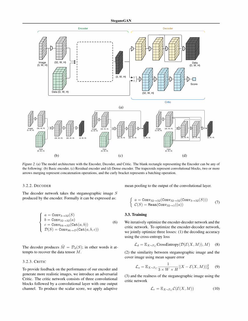
Figure 2. (a) The model architecture with the Encoder, Decoder, and Critic. The blank rectangle representing the Encoder can be any ofthe following: (b) Basic encoder, (c) Residual encoder and (d) Dense encoder. The trapezoids represent convolutional blocks, two or morearrows merging represent concatenation operations, and the curly bracket represents a batching operation.

3.2.2. DECODER

The decoder network takes the steganographic image Sproduced by the encoder. Formally it can be expressed as:

a = Conv3→32(S)b = Conv32→32(a)c = Conv64→32(Cat(a, b))D(S) = Conv96→D(Cat(a, b, c))

(6)

The decoder produces M = Dd(S); in other words it at-tempts to recover the data tensor M .

3.2.3. CRITIC

To provide feedback on the performance of our encoder andgenerate more realistic images, we introduce an adversarialCritic. The critic network consists of three convolutionalblocks followed by a convolutional layer with one outputchannel. To produce the scalar score, we apply adaptive

mean pooling to the output of the convolutional layer.

{a = Conv32→32(Conv32→32(Conv3→32(S)))C(S) = Mean(Conv32→1((a))

(7)

3.3. Training

We iteratively optimize the encoder-decoder network and thecritic network. To optimize the encoder-decoder network,we jointly optimize three losses: (1) the decoding accuracyusing the cross-entropy loss

Ld = EX∼PCCrossEntropy(D(E(X,M)),M) (8)

(2) the similarity between steganographic image and thecover image using mean square error

Ls = EX∼PC

1

3×W ×H||X − E(X,M)||22 (9)

(3) and the realness of the steganographic image using thecritic network

Lr = EX∼PCC(E(X,M)) (10)

SteganoGAN

The training objective is to

minimize Ld + Ls + Lr. (11)

To train the critic network, we minimize the Wassersteinloss

Lc =EX∼PCC(X)

− EX∼PCC(E(X,M)) (12)

During every iteration, we match each cover image C witha data tensor M , which consists of a randomly generatedsequence ofD×W×H bits sampled from a Bernoulli distri-bution M ∼ Ber(0.5). In addition, we apply standard dataaugmentation procedures including horizontal flipping andrandom cropping to cover image C in our pre-processingpipeline. We use the Adam optimizer with learning rate1e−4, clip our gradient norm to 0.25, clip the critic weightsto [−0.1, 0.1], and train for 32 epochs.

4. Evaluation MetricsSteganography algorithms are evaluated along three axes:the amount of data that can be hidden in an image, a.k.a ca-pacity, the similarity between the cover and steganographyimage, a.k.a distortion, and the ability to avoid detectionby steganalysis tools, a.k.a secrecy. This section describessome metrics for evaluating the performance of our modelalong these axes.

Reed Solomon Bits Per Pixel: Measuring the effectivenumber of bits that can be conveyed per pixel is non-trivialin our setup since the ability to recover a hidden bit is heavilydependent on the model and the cover image, as well as themessage itself.

To model this situation, suppose that a given model incor-rectly decodes a bit with probability p. It is tempting tojust multiply the number of bits in the data tensor by theaccuracy 1− p and report that value as the relative payload.Unfortunately, that value is actually meaningless – it allowsyou to estimate the number of bits that have been correctlydecoded, but does not provide a mechanism for recoveringfrom errors or even identifying which bits are correct.

Therefore, to get an accurate estimate of the relative payloadof our technique, we turn to Reed-Solomon codes. Reed-Solomon error-correcting codes are a subset of linear blockcodes which offer the following guarantee: Given a messageof length k, the code can generate a message of length nwhere n ≥ k such that it can recover from n−k

2 errors (Reed& Solomon, 1960). This implies that given a steganographyalgorithm which, on average, returns an incorrect bit withprobability p, we would want the number of incorrect bits

to be less than or equal to the number of bits we can correct:

p · n ≤ n− k2

(13)

The ratio k/n represents the average number of bits of ”real”data we can transmit for each bit of ”message” data; then,from (13), it follows that the ratio is less than or equal to1− 2p. As a result, we can measure the relative payload ofour steganographic technique by multiplying the number ofbits we attempt to hide in each pixel by the ratio to obtainthe ”real” number of bits that is transmitted and recovered.

We refer to this metric as Reed-Solomon bits-per-pixel (RS-BPP), and note that it can be directly compared againsttraditional steganographic techniques since it represents theaverage number of bits that can be reliably transmitted in animage divided by the size of the image.

Peak Signal to Noise Ratio: In addition to measuring therelative payload, we also need to measure the quality of thesteganographic image. One widely-used metric for measur-ing image quality is the peak signal-to-noise ratio (PSNR).This metric is designed to measure image distortions andhas been shown to be correlated with mean opinion scoresproduced by human experts (Wang et al., 2004).

Given two images X and Y of size (W ,H) and a scalingfactor sc which represents the maximum possible differencein the numerical representation of each pixel2, the PSNR isdefined as a function of the mean squared error (MSE):

MSE =1

WH

W∑i=1

H∑j=1

(Xi,j − Yi,j)2, (14)

PSNR = 20 · log10(sc)− 10 · log10(MSE) (15)

Although PSNR is widely used to evaluate the distortionproduced by steganography algorithms, (Almohammad &Ghinea, 2010) suggests that it may not be ideal for com-parisons across different types of steganography algorithms.Therefore, we introduce another metric to help us evaluateimage quality: the structural similarity index.

Structural Similarity Index: In our experiments, we alsoreport the structural similarity index (SSIM) between thecover image and the steganographic image. SSIM is widelyused in the broadcast industry to measure image and videoquality (Wang et al., 2004). Given two images X and Y ,the SSIM can be computed using the means, µX and µY ,

2For example, if the images are represented as floating pointnumbers in [−1.0, 1.0], then sc = 2.0 since the maximum differ-ence between two pixels is achieved when one is 1.0 and the otheris −1.0.

SteganoGAN

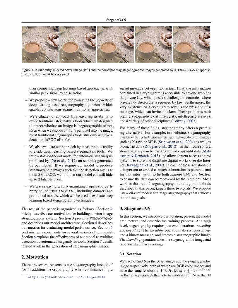
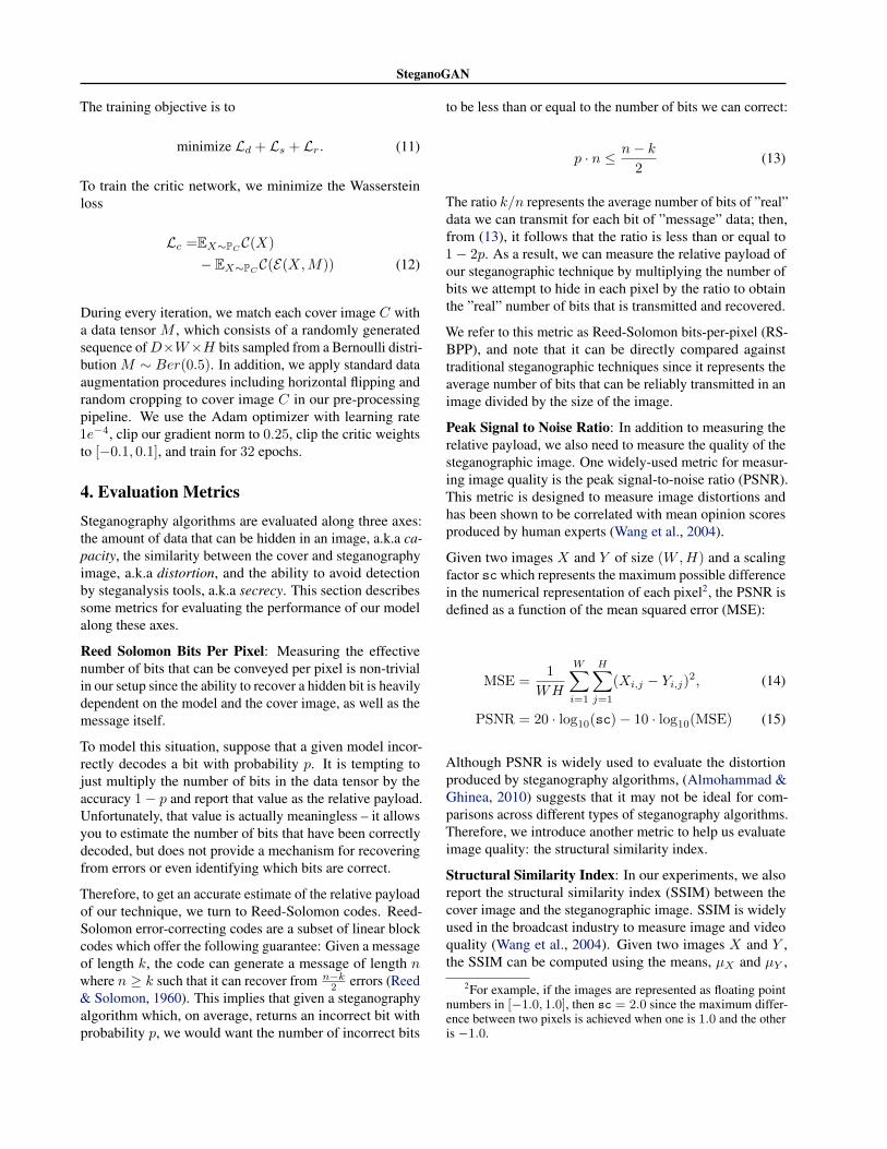
Figure 3. Randomly selected pairs of cover (left) and steganographic (right) images from the COCO dataset which embeds random binarydata at the maximum payload of 4.4 bits-per-pixel.

variances, σ2X and σ2

Y , and covariance σ2XY of the images

as shown below:

SSIM =(2µXµY + k1R)(2σXY + k2R)

(µ2X + µ2

Y + k1R)(σ2X + σ2

Y + k2R)(16)

The default configuration for SSIM uses k1 = 0.01 andk2 = 0.03 and returns values in the range [−1.0, 1.0] where1.0 indicates the images are identical.

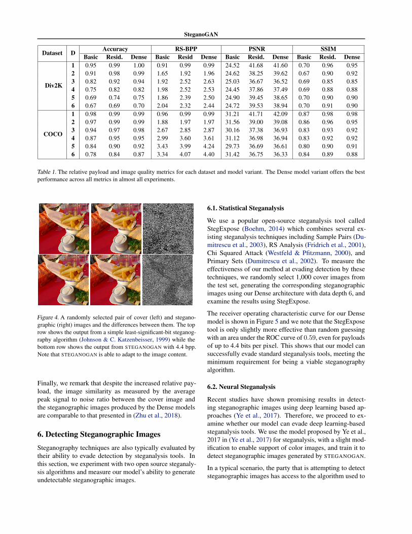
5. Results and AnalysisWe use the Div2k (Agustsson & Timofte, 2017) and COCO(Lin et al., 2014) datasets to train and evaluate our model.We experiment with each of the three model variants dis-cussed in Section 3 and train them with 6 different datadepths D ∈ {1, 2, ..., 6}. The data depth D represents the“target” bits per pixel so the randomly generated data tensorhas shape D x W x H .

We use the default train/test split proposed by the creatorsof the Div2K and COCO data sets in our experiments, andwe report the average RS-BPP, PSNR, and SSIM on thetest set in Table 1. Our models are trained on GeForce GTX1080 GPUs. The wall clock time per epoch is approximately10 minutes for Div2K and 2 hours for COCO.

After training our model, we compute the expected accuracyon a held-out test set and adjust it using the Reed-Solomon

coding scheme discussed in Section 4 to produce our bits-per-pixel metric, shown in Table 1 under RS-BPP. We pub-licly released the pre-trained models for all the experimentsshown in this table on AWS S33.

The results from our experiments are shown in Table 1 –each of the metrics is computed on a held-out test set ofimages that is not shown to the model during training. Notethat there is an unavoidable tradeoff between the relativepayload and the image quality measures; assuming we arealready on the Pareto frontier, an increased relative payloadwould inevitably result in a decreased similarity.

We immediately observe that all variants of our model per-form better on the COCO dataset than the Div2K dataset.This can be attributed to differences in the type of contentphotographed in the two datasets. Images from the Div2Kdataset tend to contain open scenery, while images fromthe COCO dataset tend to be more cluttered and containmultiple objects, providing more surfaces and textures forour model to successfully embed data.

In addition, we note that our dense variant shows the bestperformance on both relative payload and image quality,followed closely by the residual variant which shows com-parable image quality but a lower relative payload. Thebasic variant offers the worst performance across all metrics,achieving relative payloads and image quality scores thatare 15-25% lower than the dense variant.

3http://steganogan.s3.amazonaws.com/

SteganoGAN

Dataset D Accuracy RS-BPP PSNR SSIMBasic Resid. Dense Basic Resid Dense Basic Resid. Dense Basic Resid. Dense

Div2K

1 0.95 0.99 1.00 0.91 0.99 0.99 24.52 41.68 41.60 0.70 0.96 0.952 0.91 0.98 0.99 1.65 1.92 1.96 24.62 38.25 39.62 0.67 0.90 0.923 0.82 0.92 0.94 1.92 2.52 2.63 25.03 36.67 36.52 0.69 0.85 0.854 0.75 0.82 0.82 1.98 2.52 2.53 24.45 37.86 37.49 0.69 0.88 0.885 0.69 0.74 0.75 1.86 2.39 2.50 24.90 39.45 38.65 0.70 0.90 0.906 0.67 0.69 0.70 2.04 2.32 2.44 24.72 39.53 38.94 0.70 0.91 0.90

COCO

1 0.98 0.99 0.99 0.96 0.99 0.99 31.21 41.71 42.09 0.87 0.98 0.982 0.97 0.99 0.99 1.88 1.97 1.97 31.56 39.00 39.08 0.86 0.96 0.953 0.94 0.97 0.98 2.67 2.85 2.87 30.16 37.38 36.93 0.83 0.93 0.924 0.87 0.95 0.95 2.99 3.60 3.61 31.12 36.98 36.94 0.83 0.92 0.925 0.84 0.90 0.92 3.43 3.99 4.24 29.73 36.69 36.61 0.80 0.90 0.916 0.78 0.84 0.87 3.34 4.07 4.40 31.42 36.75 36.33 0.84 0.89 0.88

Table 1. The relative payload and image quality metrics for each dataset and model variant. The Dense model variant offers the bestperformance across all metrics in almost all experiments.

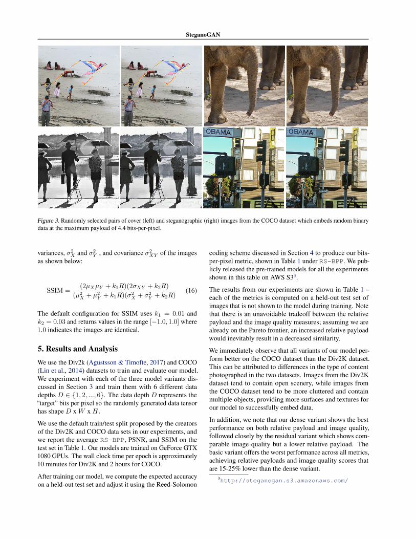
Figure 4. A randomly selected pair of cover (left) and stegano-graphic (right) images and the differences between them. The toprow shows the output from a simple least-significant-bit steganog-raphy algorithm (Johnson & C. Katzenbeisser, 1999) while thebottom row shows the output from STEGANOGAN with 4.4 bpp.Note that STEGANOGAN is able to adapt to the image content.

Finally, we remark that despite the increased relative pay-load, the image similarity as measured by the averagepeak signal to noise ratio between the cover image andthe steganographic images produced by the Dense modelsare comparable to that presented in (Zhu et al., 2018).

6. Detecting Steganographic ImagesSteganography techniques are also typically evaluated bytheir ability to evade detection by steganalysis tools. Inthis section, we experiment with two open source steganaly-sis algorithms and measure our model’s ability to generateundetectable steganographic images.

6.1. Statistical Steganalysis

We use a popular open-source steganalysis tool calledStegExpose (Boehm, 2014) which combines several ex-isting steganalysis techniques including Sample Pairs (Du-mitrescu et al., 2003), RS Analysis (Fridrich et al., 2001),Chi Squared Attack (Westfeld & Pfitzmann, 2000), andPrimary Sets (Dumitrescu et al., 2002). To measure theeffectiveness of our method at evading detection by thesetechniques, we randomly select 1,000 cover images fromthe test set, generating the corresponding steganographicimages using our Dense architecture with data depth 6, andexamine the results using StegExpose.

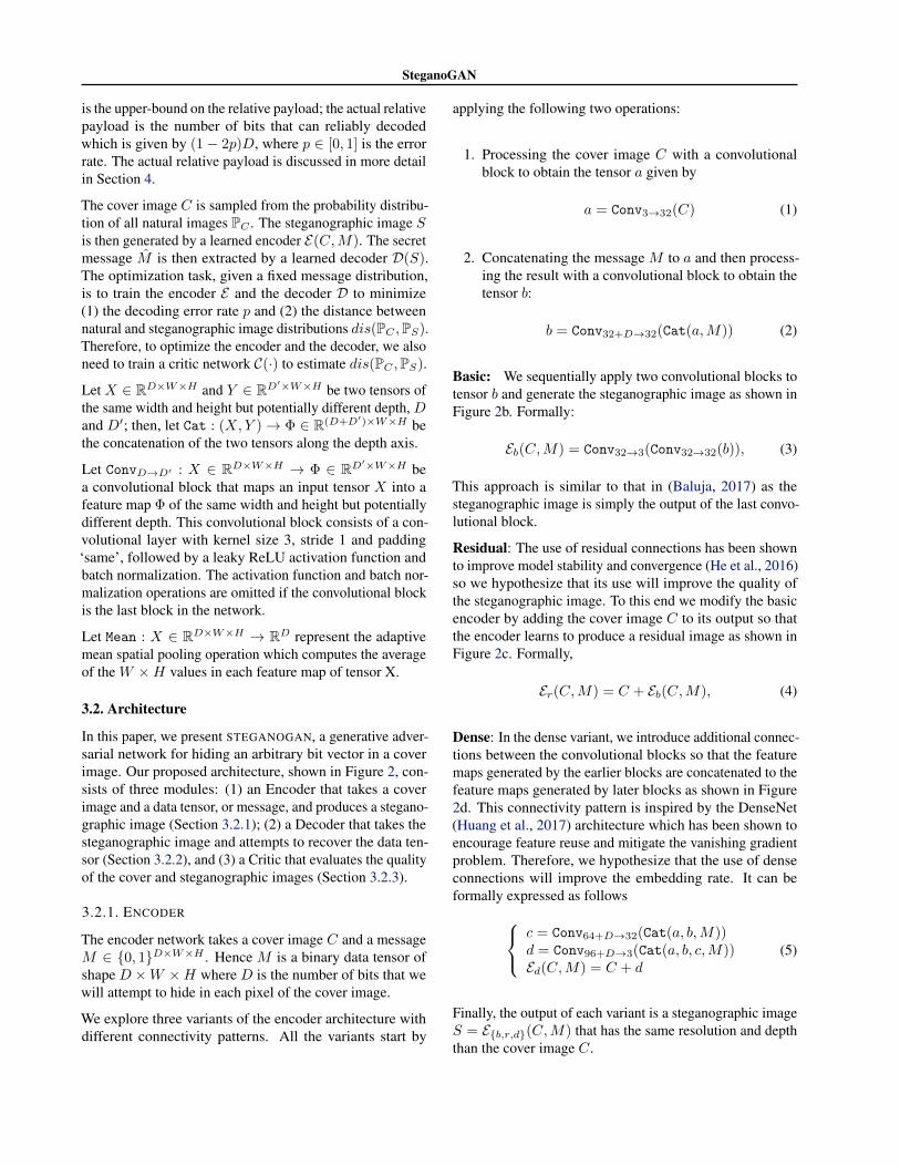
The receiver operating characteristic curve for our Densemodel is shown in Figure 5 and we note that the StegExposetool is only slightly more effective than random guessingwith an area under the ROC curve of 0.59, even for payloadsof up to 4.4 bits per pixel. This shows that our model cansuccessfully evade standard steganalysis tools, meeting theminimum requirement for being a viable steganographyalgorithm.

6.2. Neural Steganalysis

Recent studies have shown promising results in detect-ing steganographic images using deep learning based ap-proaches (Ye et al., 2017). Therefore, we proceed to ex-amine whether our model can evade deep learning-basedsteganalysis tools. We use the model proposed by Ye et al.,2017 in (Ye et al., 2017) for steganalysis, with a slight mod-ification to enable support of color images, and train it todetect steganographic images generated by STEGANOGAN.

In a typical scenario, the party that is attempting to detectsteganographic images has access to the algorithm used to

SteganoGAN

0 0.2 0.4 0.6 0.8 10

0.2

0.4

0.6

0.8

1

False Positive Rate

True

Posi

tive

Rat

e

Figure 5. The receiver operating characteristic (ROC) curve pro-duced by the StegExpose library for a set of 1000 steganographicimages generated using the Dense architecture with a data depthof 6. The StegExpose library includes multiple steganalysis toolsincluding SamplePairs (Dumitrescu et al., 2003), RSAnalysis(Fridrich et al., 2001), ChiSquaredAttack (Westfeld & Pfitz-mann, 2000), and PrimarySets (Dumitrescu et al., 2002). Thetool achieves an auROC of 0.59.

create them - in our case, an instance of STEGANOGANwhich is parameterized by the pretrained model weights butnot the exact model. Using the Dense architecture fromSection 3.2.1 and the COCO dataset, we attempt to replicatethis scenario with the following experimental setup:

1. We train N instances of the Dense STEGANOGAN ar-chitecture with different random seeds.

2. For each of these trained models, we generate a set of1,000 steganographic images.

3. Holding out the images generated by the N th model asa test set, we train the steganalysis model proposed in(Ye et al., 2017) on increasing subsets of the remainingimages {1}, {1, 2}, {1, 2, 3}, ..., {1, 2, 3, ...,N − 1}.

4. We repeat each experiment 3 times and report the aver-age area under the receiver operating curve in Figure 6.

This emulates a realistic setting - the party creating the auto-matic detection model will not have access to the specificSTEGANOGAN model in use, but may have access to thesoftware used to train the models. Therefore, we pose thefollowing question: If the external party does not know thespecific model weights but does know the algorithm forgenerating models, can they detect steganographic imagesgenerated by STEGANOGAN?

Figure 6 shows the performance of our detector for variousrelative payloads and training set sizes. First, we note that

1 2 3 4 5 6 70.5

0.6

0.7

0.8

0.9

1

Number of Instances

auR

OC

D = 1, RS-BPP = 1.0 D = 2, RS-BPP = 2.0D = 3, RS-BPP = 2.9 D = 4, RS-BPP = 3.6D = 5, RS-BPP = 4.2 D = 6, RS-BPP = 4.4

Figure 6. This plot shows the performance of the steganographydetector on a held-out test set. The x-axis indicates the number ofdifferent STEGANOGAN instances that were used, while the y-axisindicates the area under the ROC curve.

the detector performance, as measured by the area underthe receiver operating characteristic (auROC), increases aswe increase the number of bits-per-pixel encoded in theimage. In addition, we highlight the fact there is no cleartrend in the area under the ROC curve as we increase thenumber of STEGANOGAN models used for training. Thissuggests that the external party will have a difficult timebuilding a model which can detect steganographic imagesgenerated by STEGANOGAN without knowing the exactmodel parameters.

Finally, we compare the detection error for images generatedby STEGANOGAN against those reported by (Ye et al., 2017)on images generated by three state-of-the-art steganographyalgorithms: WOW (Holub & Fridrich, 2012), S-UNIWARD(Holub et al., 2014), and HILL (Li et al., 2014). Note thatthese techniques are evaluated on different dataset and assuch, the results are only approximate estimates of the actualrelative payload achievable on a particular dataset. For afixed detection error rate of 20%, we find that WOW is ableto encode up to 0.3 bpp, S-UNIWARD is able to encodeup to 0.4 bpp, HILL is able to encode up to 0.5 bpp, andSTEGANOGAN is able to encode up to 2.0 bpp.

7. Related WorkIn this section, we describe a few traditional approaches toimage steganography and then discuss recent approachesdeveloped using deep learning.

SteganoGAN

7.1. Traditional Approaches

A standard algorithm for image steganography is ”HighlyUndetectable steGO” (HUGO), a cost function-based al-gorithm which uses handcrafted features to measure thedistortion introduced by modifying the pixel value at a par-ticular location in the image. Given a set of N bits to beembedded, HUGO uses the distortion function to identifythe top N pixels that can be modified while minimizing thetotal distortion across the image (Pevny et al., 2010).

Another approach is the JSteg algorithm, which is designedspecifically for JPEG images. JPEG compression works bytransforming the image into the frequency domain usingthe discrete cosine transform and removing high-frequencycomponents, resulting in a smaller image file size. JSteguses the same transformation into the frequency domain,but modifies the least significant bits of the frequency coef-ficients (Li et al., 2011).

7.2. Deep Learning for Steganography

Deep learning for image steganography has recently beenexplored in several studies, all showing promising re-sults. These existing proposals range from training neuralnetworks to integrate with and improve upon traditionalsteganography techniques (Tang et al., 2017) to completeend-to-end convolutional neural networks which use adver-sarial training to generate convincing steganographic images(Hayes & Danezis, 2017; Zhu et al., 2018).

Hiding images vs. arbitrary data: The first set of deeplearning approaches to steganography were (Baluja, 2017;Wu et al., 2018). Both (Baluja, 2017) and (Wu et al., 2018)focus solely on taking a secret image and embedding itinto a cover image. Because this task is fundamentallydifferent from that of embedding arbitrary data, it is difficultto compare these results to those achieved by traditionalsteganography algorithms in terms of the relative payload.

Natural images such as those used in (Baluja, 2017) and(Wu et al., 2018) exhibit strong spatial correlations, andconvolutional neural networks trained to hide images inimages would take advantage of this property. Therefore, amodel that is trained in such a manner cannot be applied toarbitrary data.

Adversarial training: The next set of approaches for imagesteganography are (Hayes & Danezis, 2017; Zhu et al., 2018)which make use of adversarial training techniques. The keydifferences between these approaches and our approach arethe loss functions used to train the model, the architectureof the model, and how data is presented to the network.

The method proposed by (Hayes & Danezis, 2017) can onlyoperate on images of a fixed size. Their approach involvesflattening the image into a vector, concatenating the data

vector to the image vector, and applying feedfoward, reshap-ing, and convolutional layers. They use the mean squarederror for the encoder, the cross entropy loss for the discrim-inator, and the mean squared error for the decoder. Theyreport that image quality suffers greatly when attempting toincrease the number of bits beyond 0.4 bits per pixel.

The method proposed by (Zhu et al., 2018) uses the sameloss functions as (Hayes & Danezis, 2017) but makeschanges to the model architecture. Specifically, they “repli-cate the message spatially, and concatenate this messagevolume to the encoders intermediary representation.” Forexample, in order to hide k bits in an N ×N image, theywould create a tensor of shape (k,N ,N) where the datavector is replicated at each spatial location.

This design allows (Zhu et al., 2018) to handle arbitrarysized images but cannot effectively scale to higher relativepayloads. For example, to achieve a relative payload of 1 bitper pixel in a typical image of size 360× 480, they wouldneed to manipulate a data tensor of size (172800, 360, 480).Therefore, due to the excessive memory requirements, thismodel architecture cannot effectively scale to handle largerelative payloads.

8. ConclusionIn this paper, we introduced a flexible new approach to im-age steganography which supports different-sized cover im-ages and arbitrary binary data. Furthermore, we proposed anew metric for evaluating the performance of deep-learningbased steganographic systems so that they can be directlycompared against traditional steganography algorithms. Weexperiment with three variants of the STEGANOGAN archi-tecture and demonstrate that our model achieves higher rela-tive payloads than existing approaches while still evadingdetection.

AcknowledgementsThe authors would like to thank Plamen Valentinov Kolevand Carles Sala for their help with software support anddeveloper operations and for the helpful discussions andfeedback. Finally, the authors would like to thank Accenturefor their generous support and funding which made thisresearch possible.

ReferencesAgustsson, E. and Timofte, R. NTIRE 2017 challenge on

single image super-resolution: Dataset and study. In TheIEEE Conf. on Computer Vision and Pattern Recognition(CVPR) Workshops, July 2017.

Almohammad, A. and Ghinea, G. Stego image quality

SteganoGAN

and the reliability of psnr. In 2010 2nd InternationalConference on Image Processing Theory, Tools and Ap-plications, pp. 215–220, July 2010. doi: 10.1109/IPTA.2010.5586786.

Baluja, S. Hiding images in plain sight: Deep steganogra-phy. In Guyon, I., Luxburg, U. V., Bengio, S., Wallach,H., Fergus, R., Vishwanathan, S., and Garnett, R. (eds.),Advances in Neural Information Processing Systems 30,pp. 2069–2079. Curran Associates, Inc., 2017.

Boehm, B. StegExpose - A tool for detecting LSB steganog-raphy. CoRR, abs/1410.6656, 2014.

Conway, M. Code wars: Steganography, signals intelli-gence, and terrorism. Knowledge, Technology & Pol-icy, 16(2):45–62, Jun 2003. ISSN 1874-6314. doi:10.1007/s12130-003-1026-4.

Douglas, M., Bailey, K., Leeney, M., and Curran, K. Anoverview of steganography techniques applied to the pro-tection of biometric data. Multimedia Tools and Applica-tions, 77(13):17333–17373, Jul 2018. ISSN 1573-7721.doi: 10.1007/s11042-017-5308-3.

Dumitrescu, S., Wu, X., and Memon, N. On steganal-ysis of random lsb embedding in continuous-tone im-ages. volume 3, pp. 641 – 644 vol.3, 07 2002. doi:10.1109/ICIP.2002.1039052.

Dumitrescu, S., Wu, X., and Wang, Z. Detection of LSBsteganography via sample pair analysis. In InformationHiding, pp. 355–372, 2003. ISBN 978-3-540-36415-3.

Fridrich, J., Goljan, M., and Du, R. Reliable detection oflsb steganography in color and grayscale images. In Proc.of the 2001 Workshop on Multimedia and Security: NewChallenges, MM&#38;Sec ’01, pp. 27–30. ACM, 2001.ISBN 1-58113-393-6. doi: 10.1145/1232454.1232466.

Hayes, J. and Danezis, G. Generating steganographic im-ages via adversarial training. In NIPS, 2017.

He, K., Zhang, X., Ren, S., and Sun, J. Deep residuallearning for image recognition. IEEE Conf. on ComputerVision and Pattern Recognition (CVPR), pp. 770–778,2016.

Holub, V. and Fridrich, J. Designing steganographic dis-tortion using directional filters. 12 2012. doi: 10.1109/WIFS.2012.6412655.

Holub, V., Fridrich, J., and Denemark, T. Universal dis-tortion function for steganography in an arbitrary do-main. EURASIP Journal on Information Security, 2014(1):1, Jan 2014. ISSN 1687-417X. doi: 10.1186/1687-417X-2014-1.

Huang, G., Liu, Z., van der Maaten, L., and Weinberger,K. Q. Densely connected convolutional networks. IEEEConf. on Computer Vision and Pattern Recognition(CVPR), pp. 2261–2269, 2017.

Johnson, N. and C. Katzenbeisser, S. A survey of stegano-graphic techniques. 01 1999.

Kawaguchi, E., Maeta, M., Noda, H., and Nozaki, K. Amodel of digital contents access control system usingsteganographic information hiding scheme. In Proc. ofthe 18th Conf. on Information Modelling and KnowledgeBases, pp. 50–61, 2007. ISBN 978-1-58603-710-9.

Li, B., He, J., Huang, J., and Shi, Y. A survey on imagesteganography and steganalysis. Journal of InformationHiding and Multimedia Signal Processing, 2011.

Li, B., Wang, M., Huang, J., and Li, X. A new cost functionfor spatial image steganography. In 2014 IEEE Int. Conf.on Image Processing (ICIP), pp. 4206–4210, Oct 2014.doi: 10.1109/ICIP.2014.7025854.

Lin, T., Maire, M., Belongie, S. J., Bourdev, L. D., Girshick,R. B., Hays, J., Perona, P., Ramanan, D., Dollar, P., andZitnick, C. L. Microsoft COCO: common objects incontext. CoRR, abs/1405.0312, 2014.

Maheswari, S. U. and Hemanth, D. J. Frequency domainqr code based image steganography using fresnelet trans-form. AEU - International Journal of Electronics andCommunications, 69(2):539 – 544, 2015. ISSN 1434-8411. doi: https://doi.org/10.1016/j.aeue.2014.11.004.

Pevny, T., Filler, T., and Bas, P. Using high-dimensional im-age models to perform highly undetectable steganography.In Information Hiding, 2010.

Reed, I. S. and Solomon, G. Polynomial Codes Over CertainFinite Fields. Journal of the Society for Industrial andApplied Mathematics, 8(2):300–304, 1960.

Srinivasan, Y., Nutter, B., Mitra, S., Phillips, B., and Ferris,D. Secure transmission of medical records using highcapacity steganography. In Proc. of the 17th IEEE Sympo-sium on Computer-Based Medical Systems, pp. 122–127,June 2004. doi: 10.1109/CBMS.2004.1311702.

Tang, W., Tan, S., Li, B., and Huang, J. Automaticsteganographic distortion learning using a generativeadversarial network. IEEE Signal Processing Letters,24(10):1547–1551, Oct 2017. ISSN 1070-9908. doi:10.1109/LSP.2017.2745572.

Wang, Z., Bovik, A. C., Sheikh, H. R., and Simoncelli,E. P. Image quality assessment: from error visibility tostructural similarity. IEEE Trans. on Image Processing,13(4):600–612, April 2004. ISSN 1057-7149. doi: 10.1109/TIP.2003.819861.

SteganoGAN

Westfeld, A. and Pfitzmann, A. Attacks on steganographicsystems. In Information Hiding, pp. 61–76, 2000. ISBN978-3-540-46514-0.

Wu, P., Yang, Y., and Li, X. Stegnet: Mega image steganog-raphy capacity with deep convolutional network. FutureInternet, 10:54, 06 2018. doi: 10.3390/fi10060054.

Ye, J., Ni, J., and Yi, Y. Deep learning hierarchical rep-resentations for image steganalysis. IEEE Trans. onInformation Forensics and Security, 12(11):2545–2557,Nov 2017. ISSN 1556-6013. doi: 10.1109/TIFS.2017.2710946.

Zhu, J., Kaplan, R., Johnson, J., and Fei-Fei, L. HiDDeN:Hiding data with deep networks. CoRR, abs/1807.09937,2018.