Computer Science Department, Dartmouth College, Hanover, NH 03755, USA {kimo, lsw, farid}@cs.dartmouth.edu
ABSTRACT
Digital audio provides a suitable cover for high-throughput steganography. At 16 bits per sample and sampled at a rate of 44,100 Hz, digital audio has the bit-rate to support large messages. In addition, audio is often transient and unpredictable, facilitating the hiding of messages. Using an approach similar to our universal image steganalysis, we show that hidden messages alter the underlying statistics of audio signals. Our statistical model begins by building a linear basis that captures certain statistical properties of audio signals. A low-dimensional statistical feature vector is extracted from this basis representation and used by a non-linear support vector machine for classification. We show the efficacy of this approach on LSB embedding and Hide4PGP. While no explicit assumptions about the content of the audio are made, our technique has been developed and tested on high-quality recorded speech.
1. INTRODUCTION
Over the past few years, increasingly sophisticated techniques for information hiding (steganography) have been rapidly developing (see1–3 for general reviews). These developments, along with high-resolution carriers, pose significant chal- lenges to detecting the presence of hidden messages. There is, nevertheless, a growing literature on steganalysis. 4–7 While much of this work has been focused on detecting steganography within digital images, digital audio is a cover medium ca- pable of supporting high-throughput steganography; sampled at 44,100 Hz with 16 bits per sample, a single channel of CD quality audio has a bit-rate of 706 kilobits per second. In addition, audio is often transient and unpredictable, facilitating the hiding of messages.8–10
In previous work,7, 11 we showed that a statistical model based on first- and higher-order wavelet statistics can discrim- inate between images with and without hidden messages, regardless of the underlying embedding algorithm (i.e., universal steganalysis). We have discovered, however, that this same statistical model is not appropriate for audio steganalysis. The reason, we believe, is that the earlier model captures statistical regularities inherent to the spatial composition of images that are simply not present in audio. As such, we have developed a new statistical model that seems to capture certain statistical regularities of audio signals. Although in many ways different, this statistical model and subsequent analysis of audio signals follows the same theme as our earlier image steganalysis work.
Our statistical model begins by decomposing an audio signal using basis functions that are localized in both time and frequency (analogous to a wavelet decomposition). As before, we collect a number of statistics from this decomposition, and use a non-linear support vector machine for classification. This approach is tested on two types of steganography, least significant bit (LSB) embedding and Hide4PGP.12 While no explicit assumptions about the content of the audio are made, our technique has been developed and tested on high-quality recorded speech.
2. METHODS
We first describe the model used to capture statistical regularities of audio signals. This model, coupled with a non-linear support vector machine, is then used to differentiate between clean and stego audio signals.
2.1. Statistical Model
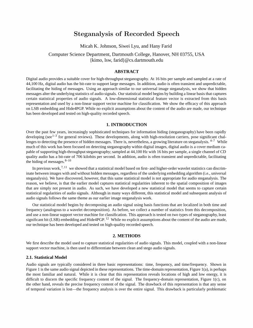
Audio signals are typically considered in three basic representations: time, frequency, and time/frequency. Shown in Figure 1 is the same audio signal depicted in these representations. The time-domain representation, Figure 1(a), is perhaps the most familiar and natural. While it is clear that this representation reveals locations of high and low energy, it is difficult to discern the specific frequency content of the signal. The frequency-domain representation, Figure 1(c), on the other hand, reveals the precise frequency content of the signal. The drawback of this representation is that any sense of temporal variation is lost—the frequency analysis is over the entire signal. This drawback is particularly problematic
(a) A
m pl
itu de
0
1
10
20
−40
−20
0
Frequency (kHz)
Figure 1. Three representations of an audio signal: (a) time; (b) time/frequency; and (c) frequency: (a) the signal in the time-domain is represented in terms of basis functions that are highly localized in time; (b) the signal in the time/frequency-domain is represented in terms of basis functions that partially localized in both time and frequency; and (c) the signal in the frequency-domain is represented in terms of basis functions that are highly localized in frequency. For purposes of visualization, the time/frequency representation in panel (b) is gamma-corrected (γ = 0.75).
for audio signals where the frequency properties of the signal can vary dramatically over time. The time/frequency- domain representation, Figure 1(b), overcomes some of the disadvantages of a strictly time- or strictly frequency-domain representation. In this representation, a signal is represented in terms of basis functions that are localized in both time and frequency.13
2.1.1. STFT
The short-time Fourier transform (STFT) is perhaps the most common time/frequency decomposition for audio signals (wavelets are another popular decomposition). Let f [n] be a discrete signal of length F . Recall that the Fourier transform of f [n] is given by:
F [ω] = F−1∑
f [n]e−i2πωn/F . (1)
The STFT is computed by applying the Fourier transform to shorter time segments of the signal. The STFT of f [n] is given by:
FS[ω, t] = M−1∑
n=0
h[n] f [n + t]e−i2πωn/M , (2)
where h[n] is a window function of length M (e.g., a Gaussian, Hanning, or sine window). The offset parameter t is usually chosen to be less than M so that the original signal f [n] can be reconstructed from the STFT, F S[ω, t]. As with
STFTSTFT STFTSTFTSTFTSTFT
smks1k smis1i . . .
gi [n]gk[n]g1[n]
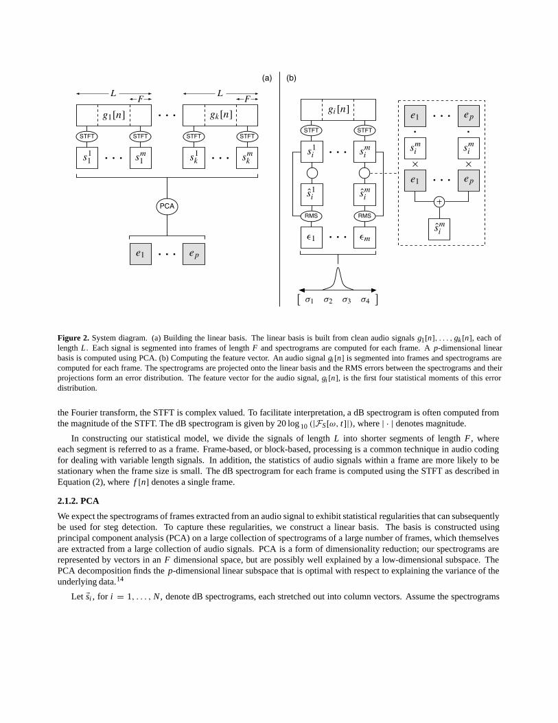
Figure 2. System diagram. (a) Building the linear basis. The linear basis is built from clean audio signals g1[n], . . . , gk [n], each of length L . Each signal is segmented into frames of length F and spectrograms are computed for each frame. A p-dimensional linear basis is computed using PCA. (b) Computing the feature vector. An audio signal gi [n] is segmented into frames and spectrograms are computed for each frame. The spectrograms are projected onto the linear basis and the RMS errors between the spectrograms and their projections form an error distribution. The feature vector for the audio signal, gi [n], is the first four statistical moments of this error distribution.
the Fourier transform, the STFT is complex valued. To facilitate interpretation, a dB spectrogram is often computed from the magnitude of the STFT. The dB spectrogram is given by 20 log 10 (|FS[ω, t]|), where | · | denotes magnitude.
In constructing our statistical model, we divide the signals of length L into shorter segments of length F , where each segment is referred to as a frame. Frame-based, or block-based, processing is a common technique in audio coding for dealing with variable length signals. In addition, the statistics of audio signals within a frame are more likely to be stationary when the frame size is small. The dB spectrogram for each frame is computed using the STFT as described in Equation (2), where f [n] denotes a single frame.
2.1.2. PCA
We expect the spectrograms of frames extracted from an audio signal to exhibit statistical regularities that can subsequently be used for steg detection. To capture these regularities, we construct a linear basis. The basis is constructed using principal component analysis (PCA) on a large collection of spectrograms of a large number of frames, which themselves are extracted from a large collection of audio signals. PCA is a form of dimensionality reduction; our spectrograms are represented by vectors in an F dimensional space, but are possibly well explained by a low-dimensional subspace. The PCA decomposition finds the p-dimensional linear subspace that is optimal with respect to explaining the variance of the underlying data.14
Let si , for i = 1, . . . , N , denote dB spectrograms, each stretched out into column vectors. Assume the spectrograms
are of length F .∗ The overall mean of these dB spectrograms is given by:
µ = 1
A F × N zero-meaned data matrix is constructed as follows:
S = ( s1 − µ s2 − µ · · · sN − µ ) . (4)
The F × F (scaled) covariance matrix† of this data matrix is given by:
C = SST . (5)
The principal components of the data matrix are the eigenvectors of the covariance matrix (i.e., Ce j = λ j e j ), where the eigenvalue λ j is proportional to the variance of the original data along the principal axis e j . The inherent dimensionality of each spectrogram si is reduced from F to p by reconstructing s i in terms of the largest p eigenvalue-eigenvectors:
si = p∑
j=1
(e j · si )e j , (6)
where ‘·’ denotes inner product. The resulting spectrogram s i is a representation of si in the p-dimensional subspace span{e1, . . . , ep}.
The statistical regularities in an audio signal are embodied by quantifying how well the audio signal can be modeled using the linear subspace. The audio signal is first partitioned into multiple frames. The dB spectrogram of each frame is computed and reconstructed in terms of the p-dimensional linear subspace. The root mean square (RMS) error between each frame’s spectrogram and its subspace representation is computed by:
1√ F
si − si . (7)
The RMS errors for all the frames of an audio signal yield an error distribution which can be characterized by the first four statistical moments: mean, variance, skewness, and kurtosis. These four statistics form the feature vector used for differentiating between clean and stego audio.
Shown in Figure 2 is a complete system diagram. Shown in panel (a) is the construction of the linear basis using PCA, and in panel (b) is the extraction of the statistical feature vector.
2.2. Classification
Having collected the statistical feature vectors from both clean and stego audio signals, a classifier is required that can differentiate between these two classes of signals. As with our earlier work on detecting steganography in digital im- ages,7 a non-linear support vector machine (SVM)15, 16 is employed. We find that non-linear classifiers offer significant improvements in detection accuracy over linear techniques.
We briefly describe linear and non-linear SVMs. Let x i denote the feature vector, and let yi denote its class label (e.g., yi = +1 if xi corresponds to a clean audio signal, and yi = −1 if xi corresponds to a stego audio signal). In a linear SVM, we seek a linear decision function f (·) determined by a unit vector w and an offset b as:
f (x) = sgn( w · x − b) , (8)
∗Using a window function that allows 50% overlap, the number of values in a dB spectrogram of a real-valued signal can be the same as the frame size.
†If F is larger than N , the Gram matrix, Cg = ST S should be considered to reduce computational complexity. The non-zero eigenvalues of the Gram matrix are the same as those of the covariance matrix C from Equation (5). An eigenvector e of the covariance matrix C can be computed from the eigenvectors eg of the Gram matrix Cg as e = Seg .
γ
b
(b)
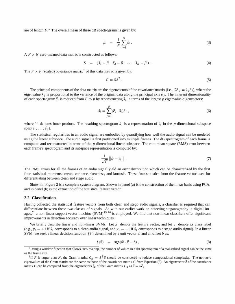
Figure 3. Linear SVM. (a) For linearly separable data, SVM classification seeks the surface (dashed line) that maximizes the classifica- tion margin γ . (b) For linearly non-separable data, slack variables ξi are introduced to allow for violations from linear separation.
where f (x) outputs +1 for positive-labeled data points and −1 for negative-labeled data points. The decision function f (·) is estimated by maximizing the classification margin γ subject to the following constraints:
w · xi − b ≥ γ if yi = +1 ,
w · xi − b ≤ −γ if yi = −1 ,
w = 1 .
(9)
These constraints force all the data to be outside the margin region and force w to be a unit vector. Shown in Figure 3(a) is an example where the classes of data to be separated are depicted as filled and empty circles. The classification margin γ is the distance that the classification surface can translate while still separating the two classes of data. The SVM optimization problem is to maximize γ subject to the constraints in Equation (9). This optimization problem can be transformed into a constrained convex quadratic programming problem and solved using efficient iterative algorithms. 15
In the case where the data is not linearly separable, the optimization problem is adjusted to tolerate some classification errors, as shown in Figure 3(b). Specifically, slack variables ξ i are introduced for each data point x i to indicate its violation from a linear separation. The constraints of Equation (9) are changed accordingly to:
w · xi − b ≥ γ − ξi if yi = +1 ,
w · xi − b ≤ −γ + ξi if yi = −1 ,
w = 1 ,
ξi ≥ 0 .
(10)
The overall classification error is measured by the sum of the slack variables. To reflect the compromise between minimiz- ing the classification error and maximizing the classification margin, the objective function is changed from maximizing γ
to maximizing the following expression:
γ − C N∑
where C > 0 is a penalty on the classification errors.
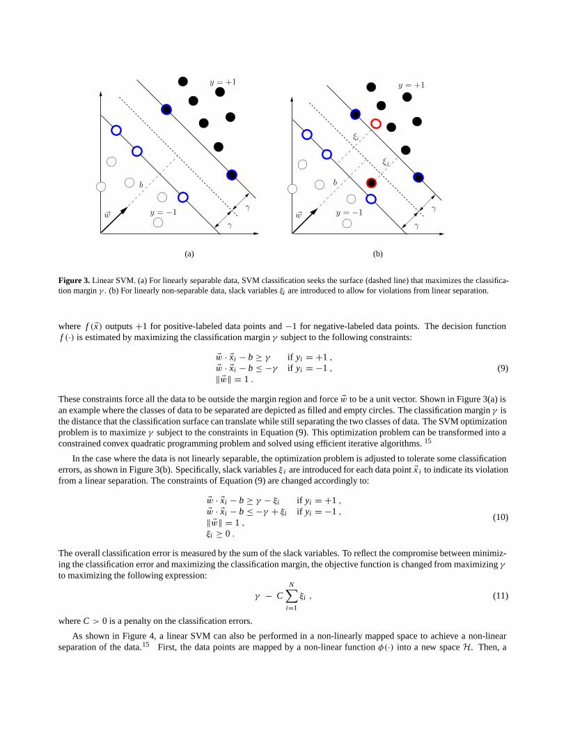
As shown in Figure 4, a linear SVM can also be performed in a non-linearly mapped space to achieve a non-linear separation of the data.15 First, the data points are mapped by a non-linear function φ(·) into a new space H. Then, a
y = −1
y = +1
y = −1
y = +1
φ(·)
HRd
Figure 4. Non-linear SVM classification. The original data points in Rd are mapped into H by a non-linear mapping function φ(·). Non-linear SVM classification seeks a linear classification surface in H.
linear SVM algorithm is run in H to find the linear decision function from Equation (8). A linear decision function in H corresponds to a non-linear classification surface in the original space. For computational efficiency, a kernel function that is equivalent to computing inner products of two mapped data points in H is used in the optimization algorithm.
3. RESULTS
We test our steganalysis technique on audio signals embedded with two types of steganography: LSB and Hide4PGP. The LSB embedding procedure, described below, is a variation of traditional LSB embedding to allow for high-throughput steganography. Hide4PGP is freely available steganography software that can embed large messages in WAV and BMP files.12
Our audio data comes from a database of recorded speech collected from books on CD. The database contains record- ings from 18 distinct speakers, 9 male and 9 female, and there is approximately two hours of speech per speaker. All of the audio data is CD quality: 16 bits per sample and sampled at a rate of 44,100 samples per second. The recordings were spot-checked to verify that no recording contained audible noise.
For the cover signals, 1800 ten second audio signals were randomly extracted from the database, 100 signals from each speaker. The LSB-embedded stego signals were created from the cover signals by embedding random messages of sizes 1 through 8 bits. These sizes refer to the number of bits per sample that were possibly modified. Eight-bit messages represent one extremum—the hidden messages are clearly perceptible and the SNR between the cover and message is, on average, 30 dB. Every bit lost in message size yields a 6 dB gain in SNR; the SNR for 1-bit messages is, on average, 72 dB. For many of our audio signals, 4-bit messages are imperceptible over the noise naturally present in the signals. In total, there are 14,400 LSB-embedded stego signals, 1800 signals for each message size of 1 through 8 bits.
The Hide4PGP stego signals are created from the cover signals by embedding messages at four different capacities: 25%, 50%, 75%, and 100%. Setting the capacity to 100% causes Hide4PGP to embed at 4 bits per sample. Therefore, the chosen capacities correspond to embedding at 1, 2, 3, and 4 bits per sample, respectively. There are 1800 Hide4PGP stego signals for each of the four capacities for a total of 7200 Hide4PGP stego signals.
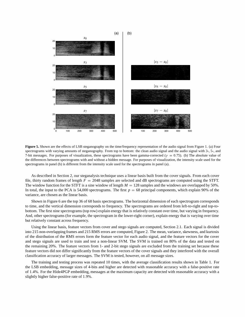
Shown in Figure 5 are the effects of LSB steganography on a 500 ms portion of the spectrogram from Figure 1. Shown in panel (a), from top to bottom, is the spectrogram, s 0, for the clean signal, and the spectrograms for 3-, 5-, and 7-bit messages, denoted as s3, s5, and s7, respectively. The effects of steganography are most noticeable in the quiet region near 400 ms. Shown in Figure 5(b) are the absolute values of the differences between the spectrograms of the signals with steganography and the spectrogram of the clean signal.
s7
s5
s3
s0
0
10
20
0
10
20
0
10
20
10
20
(a) (b)
|s7 − s0|
|s5 − s0|
|s3 − s0|
Figure 5. Shown are the effects of LSB steganography on the time/frequency representation of the audio signal from Figure 1. (a) Four spectrograms with varying amounts of steganography. From top to bottom: the clean audio signal and the audio signal with 3-, 5-, and 7-bit messages. For purposes of visualization, these spectrograms have been gamma-corrected (γ = 0.75). (b) The absolute value of the differences between spectrograms with and without a hidden message. For purposes of visualization, the intensity scale used for the spectrograms in panel (b) is different from the intensity scale used for the spectrograms in panel (a).
As described in Section 2, our steganalysis technique uses a linear basis built from the cover signals. From each cover file, thirty random frames of length F = 2048 samples are selected and dB spectrograms are computed using the STFT. The window function for the STFT is a sine window of length M = 128 samples and the windows are overlapped by 50%. In total, the input to the PCA is 54,000 spectrograms. The first p = 68 principal components, which explain 90% of the variance, are chosen as the linear basis.
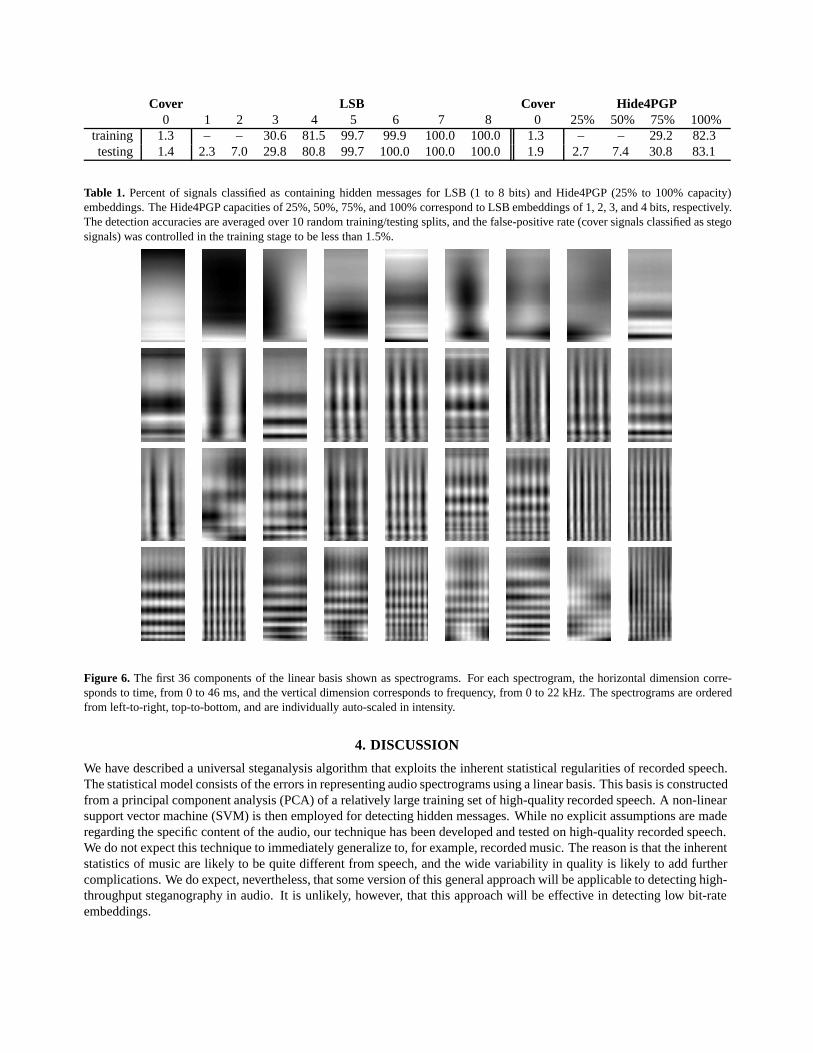
Shown in Figure 6 are the top 36 of 68 basis spectrograms. The horizontal dimension of each spectrogram corresponds to time, and the vertical dimension corresponds to frequency. The spectrograms are ordered from left-to-right and top-to- bottom. The first nine spectrograms (top row) explain energy that is relatively constant over time, but varying in frequency. And, other spectrograms (for example, the spectrogram in the lower-right corner), explain energy that is varying over time but relatively constant across frequency.
Using the linear basis, feature vectors from cover and stego signals are computed, Section 2.1. Each signal is divided into 215 non-overlapping frames and 215 RMS errors are computed, Figure 2. The mean, variance, skewness, and kurtosis of the distribution of the RMS errors form the feature vector for each audio signal, and the feature vectors for the cover and stego signals are used to train and test a non-linear SVM. The SVM is trained on 80% of the data and tested on the remaining 20%. The feature vectors from 1- and 2-bit stego signals are excluded from the training set because these feature vectors did not differ significantly from the feature vectors of the cover signals and they interfered with the overall classification accuracy of larger messages. The SVM is tested, however, on all message sizes.
The training and testing process was repeated 10 times, with the average classification results shown in Table 1. For the LSB embedding, message sizes of 4-bits and higher are detected with reasonable accuracy with a false-positive rate of 1.4%. For the Hide4PGP embedding, messages at the maximum capacity are detected with reasonable accuracy with a slightly higher false-positive rate of 1.9%.
Cover LSB Cover Hide4PGP 0 1 2 3 4 5 6 7 8 0 25% 50% 75% 100%
training 1.3 – – 30.6 81.5 99.7 99.9 100.0 100.0 1.3 – – 29.2 82.3 testing 1.4 2.3 7.0 29.8 80.8 99.7 100.0 100.0 100.0 1.9 2.7 7.4 30.8 83.1
Table 1. Percent of signals classified as containing hidden messages for LSB (1 to 8 bits) and Hide4PGP (25% to 100% capacity) embeddings. The Hide4PGP capacities of 25%, 50%, 75%, and 100% correspond to LSB embeddings of 1, 2, 3, and 4 bits, respectively. The detection accuracies are averaged over 10 random training/testing splits, and the false-positive rate (cover signals classified as stego signals) was controlled in the training stage to be less than 1.5%.
Figure 6. The first 36 components of the linear basis shown as spectrograms. For each spectrogram, the horizontal dimension corre- sponds to time, from 0 to 46 ms, and the vertical dimension corresponds to frequency, from 0 to 22 kHz. The spectrograms are ordered from left-to-right, top-to-bottom, and are individually auto-scaled in intensity.
4. DISCUSSION
We have described a universal steganalysis algorithm that exploits the inherent statistical regularities of recorded speech. The statistical model consists of the errors in representing audio spectrograms using a linear basis. This basis is constructed from a principal component analysis (PCA) of a relatively large training set of high-quality recorded speech. A non-linear support vector machine (SVM) is then employed for detecting hidden messages. While no explicit assumptions are made regarding the specific content of the audio, our technique has been developed and tested on high-quality recorded speech. We do not expect this technique to immediately generalize to, for example, recorded music. The reason is that the inherent statistics of music are likely to be quite different from speech, and the wide variability in quality is likely to add further complications. We do expect, nevertheless, that some version of this general approach will be applicable to detecting high- throughput steganography in audio. It is unlikely, however, that this approach will be effective in detecting low bit-rate embeddings.
ACKNOWLEDGMENTS
This work was supported by an Alfred P. Sloan Fellowship, an NSF CAREER Award (IIS99-83806), an NSF Infrastructure Grant (EIA-98-02068), and under Award No. 2000-DT-CX-K001 from the Office for Domestic Preparedness, U.S. De- partment of Homeland Security (points of view in this document are those of the authors and do not necessarily represent the official position of the U.S. Department of Homeland Security).
REFERENCES
1. F. A. P. Petitcolas, R. J. Anderson, and M. G. Kuhn, “Information hiding—a survey,” Proceedings of the IEEE 87, pp. 1062–1078, July 1999.
2. N. F. Johnson and S. Jajodia, “Exploring steganography: Seeing the unseen,” IEEE Computer 31(2), pp. 26–34, 1998. 3. R. J. Anderson and F. A. P. Petitcolas, “On the limits of steganography,” IEEE Journal on Selected Areas in Commu-
nications 16, pp. 474–481, May 1998. 4. J. Fridrich and M. Goljan, “Practical steganalysis of digital images—state of the art,” Proceedings of the SPIE Pho-
tonics West 4675, pp. 1–13, 2002. 5. N. F. Johnson and S. Jajodia, “Steganalysis: The investigation of hidden information,” Proceedings of the 1998 IEEE
Information Technology Conference , pp. 113–116, 1998. 6. J. Fridrich, M. Goljan, and D. Hogea, “Steganalysis of JPEG images: Breaking the F5 algorithm,” 5th International
Workshop on Information Hiding , 2002. 7. S. Lyu and H. Farid, “Detecting hidden messages using higher-order statistics and support vector machines,” 5th
International Workshop on Information Hiding , 2002. 8. A. Westfeld, “Detecting low embedding rates,” 5th International Workshop on Information Hiding , 2002. 9. S. Dumitrescu, X. Wu, and Z. Wang, “Detection of LSB steganography via sample pair analysis,” IEEE Transactions
on Signal Processing 51, pp. 1995–2007, July 2003. 10. H. Ozer, I. Avcbas, B. Sankur, and N. Memon, “Steganalysis of audio based on audio quality metrics,” Proceedings
of SPIE 5020, pp. 55–66, June 2003. 11. H. Farid, “Detecting hidden messages using higher-order statistical models,” International Conference on Image
Processing , 2002. 12. H. Repp, “Hide4PGP,” 2000. http://www.heinz-repp.onlinehome.de/Hide4PGP.htm. 13. M. Bosi and R. E. Goldberg, Introduction to Digital Audio Coding and Standards, Kluwer Academic Publishers,
2003. 14. J. E. Jackson, A User’s Guide to Principal Components, John Wiley & Sons, 2003. 15. V. N. Vapnik, The Nature of Statistical Learning Theory, Springer-Verlag, 2nd ed., 2000. 16. C. J. Burges, “A tutorial on support vector machines for pattern recognition,” Data Mining and Knowledge Discovery
2(2), pp. 121–167, 1998.