Seats, Votes, and Gerrymandering: Estimating Representation and Bias in State Legislative Redistricting

The Harvard community has made this article openly available.Please share how this access benefits you. Your story matters.

Citation Browning, Robert X., and Gary King. 1987. Seats, votes, and gerrymandering: Estimating representation andbias in state legislative redistricting. Law and Policy 9(3): 305-322.

Published Version doi:10.1111/j.1467-9930.1987.tb00413.x

Accessed February 26, 2013 10:49:26 PM EST

Citable Link http://nrs.harvard.edu/urn-3:HUL.InstRepos:4319953

Terms of Use This article was downloaded from Harvard University's DASH repository, and is made available under theterms and conditions applicable to Other Posted Material, as set forth at http://nrs.harvard.edu/urn-3:HUL.InstRepos:dash.current.terms-of-use#LAA

Seats, Votes, and Gerrymandering: Estimating Representation and Bias in

State Legislative Redistricting ROBERT X. BROWNING and GARY KING*

The Davis v. Bandemer case focused much attention on theproblem of using statistical evidence to demonstrate the existence of political gerrymandering. In this paper, we evaluate the uses and limitations of measures of the seat- votes relationship in the Bandemer case. We outline a statktical method we have developed that can be used to estimate bias and the form of representation in legislative redistricting. We apply this method to Indiana state House and Senate elections for the period 1972 to 1984 and demonstrate a maximum bias of 6.2% toward the Republicans in the House and a 2.8% bias in the Senate.

I. INTRODUCTION

In an important case decided in 1986, the U.S. Supreme Court held for the first time that the long-standing practice of political gerrymandering was justiciable (Davis v. Bandemer, 106 S.Ct. 2797 (1986)). Undoubtedly because the justices understood full well that they were venturing into the "political thicket" of which Justice Frankfurter had once warned, the Court in the same decision ruled that the appellees, the Indiana Democrats, had not met the threshold necessary to prove that gerrymandering had occurred. In this case and in the California case that almost surely will follow (Badham v. Eu), the courts are increasingly asked to consider statistical evidence purporting to show that a political party is, through the gerry- mander, unfairly disadvantaged in its ability to translate citizen votes into legislative seats.

In this paper, our goal is in part to assist the courts in their quest to understand "which statistician is more credible or less credible" (Bandemer v. Davis (603 F. Supp. 1479, 1485) (S.D. Ind. 1984)) and to provide some help in understanding the limits of seats-votes relationships as indicators of political discrimination. In the sections that follow we outline the legal background to gerrymandering cases and evaluate the statistical

* We appreciate the comments and discussions on earlier drafts of this article with Robert Bauman, Gerald Benjamin. William Browning, David Dreyer. Bernard Grofman, Christine Harrinaton. Beth Henschen, Seung-Hyun Kim, William McLauchlan. William Shaffer, and

LAW & POLICY, Vol. 9, No. 3, July 1987 @ 1987 Basil Blackwell ISSN 0265-8240 33-00

306 LA W & POLICY July 1987

requirements and problems presented by the recent Indiana redistricting case.

A statistical model we have developed (King and Browning, 1987) is used to point out problematic aspects of past research. This model can provide statistically reliable estimates of both partisan bias and the form of democratic representation. We outline this model and apply it to the historical seats-votes data for the Indiana state Senate and House of Representatives. Finally, we conclude by stressing the implications of the use of seats-votes relationships for future court cases.

11. LEGAL BACKGROUND

Prior to the Bandemer Supreme Court decision, partisan political gerry- mandering was not considered justiciable (Dixon, 1971: 32; see also, Grofman et al., 1982).' In this decision, the first argued in the term and one of the last t o be decided, the Justices were sharply divided into three groups: Those who believed that the issue was justiciable, but not proven in this case; those who believed that it was justiciable and demonstrated; and those who thought it was not justiciable. The majority opinion (written by Justice White and joined by Justices Brennan, Marshall, Blackmun, Powell, and Stevens) held that gerrymandering was a justiciable controversy rather than a "nonjusticiable political question." On the question of whether the appellees, the Indiana Democrats, had met the threshold in proving a denial of equal protection, this group of justices split. A plurality of four (White joined by Brennan, Marshall, and Blackmun) ruled that the threshold had not been met. Justice Powell, joined by Justice Stevens, dissented from this view and argued that the threshold had been met. In an opinion concurring only in the result, Justice O'Connor Goined by Chief Justice Burger and Justice Rehnquist) argued strongly against the justiciability of this issue: "The step taken today is a momentous one, that if followed in the future can only lead to political instability and judicial malaise . . . The Equal Protection Clause does not supply judicially manageable standards for resolving purely political gerrymandering claims, and no group right to an equal share of political power was ever intended by the Framers of the Fourteenth Amendment" (106 S.Ct. 2797, 2818 (1986)).

The impact of this decision is to allow other cases alleging political gerry- mandering to proceed through the courts. The most notable is the case challenging the California congressional redistricting, Badham v. Eu (see Grofman, 1985b), that essentially has been on hold since the appeal in the Indiana Bandemer decision was accepted by the high court.2 Barring changes in the Court or positions of the justices, the decisions in future cases will rest on the ability of the plaintiffs to prove that they have met the threshold test. The question that we address is the appropriateness of seats- votes statistics in establishing the required threshold.

; Browning and King SEA TS, VOTES, AND GERRYMANDERING 307

Much attention in the Bandemer debate focused on a single statistic cited by the majority in the district court decision, the difference between the percentage of statewide votes received by the democrats and the percentage of seats won in the legislature:

Most significant among these many statistical figures is the fact that in 1982 Democratic candidates for the Indiana House earned 5 1.9 percent of all votes cast across the state. However only 43 [of 1001 Democrats were elected to seats. The State argues that it is possible that this disparity is explained by the Republicans fielding better candidates or other factors that make the outcome of such elections sensitive to the interests of the voters and the issues of the day. The Court would readily concede this possibility, but the disparity between the percentage of votes and the number of seats won is, at the very least, a signal that Democrats may have been unfairly disadvantaged by the districting (603 F. Supp. at 1485).

In his dissenting opinion in the district court case, Judge Pel1 took issue with this statistic. Grofman, an expert witness for the Republicans in the Indiana case, was also critical of the district court's reliance on the seats-votes statistic:

I feel obligated to mention my own worst fear, namely, that even though statistical methods to detect gerrymandering do exist, courts will be unable to grasp the sophisticated nuances of seatshotes relationships and the need for multifaceted tests. . . . the Bandemer majority opinion is my fear come to life: It oversimplifies the relationship between the existence of seatshotes discrep- ancies and evidence of political gerrymandering (Grofman. 1985a: 159).

The Supreme Court plurality also took issue with the statistic:

Relying on a single election to prove unconstitutional discrimination is unsatis- factory. The District Court observed, and the parties do not disagree, that Indiana is a swing State. Voters sometimes prefer Democratic candidates, and sometimes Republican. . . . The District Court did not ask by what percentage the statewide Democratic vote would have had to increase to control either the House or the Senate. The appellants argue here, without a persuasive response from appellees, that had the Democratic candidates received an additional few percentage points of the votes cast statewide, they would have obtained a majority of the seats in both houses. Nor was there any finding that the 1981 reapportionment would consign the Democrats to a minority status in the Assembly throughout the 1980's or that the Democrats would have no hope of doing any better in the reapportionment that would occur after the 1990 census. Without findings of this nature, the District Court erred in concluding that the 1981 Act violated the Equal Protection Clause (106 S.Ct. at 2812).

Given these facts and findings of the Court, a more complete evaluation of the seats-votes relationship and its appropriateness as an indicator of political gerrymandering is needed.

111. EVALUATING THE EVIDENCE IN BANDEMER

Previous analyses have focused almost exclusively on data from only one election year to assess partisan bias in legislative redistricting. In this

308 LA W & POLICY July 1987

section, we make two points about this commonplace practice. First, we show that previous methods of analyzing one year are flawed. Second, we argue that even a correct analysis of one election year is inadequate to assess bias. The reason is that what appears as partisan bias may be bias, or it just may reflect a different system of fair representation. With existing statistical methods and models, results from multiple elections are needed to distinguish these two essential components.

In his dissent in the Bandemer district court decision, Judge Pel1 argued that the majority's method of analyzing the single year seats-votes relation- ship was inadequate. Along with Justicce Stevens in Karcher v. Daggett (462 U.S. 725 (1983)), Pell favored the use of a method proposed by Backstrom, Robins and Eller (1978) in which

. . . these authors suggest isolating "typical" statewide races, those concerning "relatively invisible offices," and determining the percentage of votes cast for each candidate in these races. Id. at 1131. These "typical" races more accurately reflect partisan voting strength because their outcome depends, more often than not, on straight party affiliation rather than on the personalities of the particular candidates. Id. (603 F. Supp. at 1501).

Unfortunately, as Niemi (1985: 206-207) correctly points out (see also, Grofman, 1985a: 121), Pell misapplies this methodology to Indiana. Rather than averaging a statewide base vote for 1980 and 1982 (46.8% Democratic) and comparing it to the 1982 Democratic House seats won (43%) and the Senate seats (52%), he should have calculated the number of legislative seats that would have been won if this ".normal" vote were cast in the 77 legislative districts. Neither Niemi nor Pel1 carry out this calculation, presumably because of the enormity of the task. The data must first be collected for the 4755 precincts and then aggregated within district lines into the 77 single and multi-member 1982 legislative districts. This aggregation produces the partisari balance in the simulated legislative election.

We have calculated this statistic for the 1982 ~ndiana House races. Averaging the statewide vote for two minor state offices, the auditor and clerk of the courts, we find that the statewide "normal vote" is 49.8% Dem~cra t ic .~ When aggregated into 1982 legislative districts, we find that the Democrats would win 3 1 (40.2%) of 77 districts based on this "normal" vote. Since sixteen of these districts are double or triple member districts, this translates into 38 (38%) Democratic members in the 100 member H ~ u s e . ~ Whereas Judge Pell calculated that the 46.8% Democratic "normal" vote would have elected 43 House members, we calculate that a 49.8% "normal" vote would have elected only 38 House members. Rather than the 3.8% difference he finds, we find an 11.8% difference, even larger than the 8.9% difference between the actual 51.9% of the votes and the 43 seats won.

Although the Supreme Court speculated about whether the 1982 election was atypical, the direct result of the 1981 redistricting, or simply a typical off-year election in Indiana, little attention was given to additional ~ . : ~ + - . . : . ~ i , I , . - T . ..-..-- I . . .I:. .... . I . I .... n . . C 7

Browning and King SEA TS, VOTES, AND GERR YMANDERZNG 309

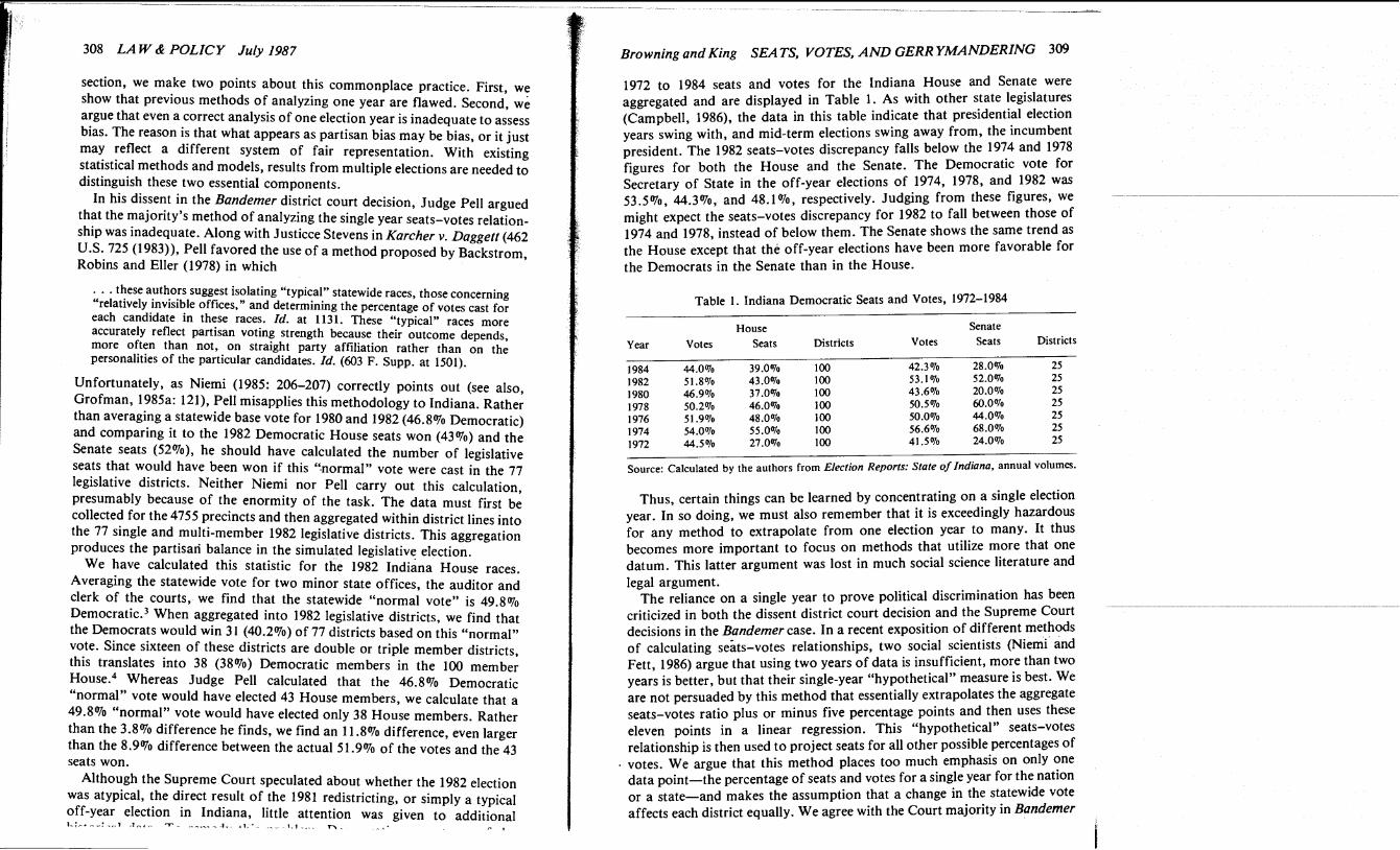
1972 to 1984 seats and votes for the Indiana House and Senate were aggregated and are displayed in Table 1. As with other state legislatures (Campbell, 1986), the data in this table indicate that presidential election years swing with, and mid-term elections swing away from, the incumbent president. The 1982 seats-votes discrepancy falls below the 1974 and 1978 figures for both the House and the Senate. The Democratic vote for Secretary of State in the off-year elections of 1974, 1978, and 1982 was 53.5%, 44.3%, and 48.1 %, respectively. Judging from these figures, we

- pppppp

might expect the seats-votes discrepancy for 1982 to fall between those of 1974 and 1978, instead of below them. The Senate shows the same trend as the House except that the off-year elections have been more favorable for the Democrats in the Senate than in the House.

Table 1. Indiana Democratic Seats and Votes, 1972-1984

House Senate Year Votes Seats Districts Votes Seats Districts

1984 44.0% 39.0% 100 42.3% 28.0% 25

1982 51.8% 43.0% 100 53.1% 52.0% 25

1980 46.9% 37.0% 100 43.6% 20.0% 25

1978 50.2% 46.0% 100 50.5% 60.0% 25 1976 51.9% 48.0% 100 50.0% 44.0% 25

1974 54.0% 55.0% 100 56.6% 68.0% 25

1972 44.5% 27.0% 100 41.5% 24.0% 25

Source: Calculated by the authors from Election Reports: State of Indiana, annual volumes.

Thus, certain things can be learned by concentrating on a single election year. In so doing, we must also remember that it is exceedingly hazardous for any method to extrapolate from one election year to many. It thus becomes more important to focus on methods that utilize more that one datum. This latter argument was lost in much social science literature and legal argument.

The reliance on a single year to prove political discrimination has been criticized in both the dissent district court decision and the Supreme Court decisions in the Bandemer case. In a recent exposition of different methods of calculating seats-votes relationships, two social scientists (Niemi and Fett, 1986) argue that using two years of data is insufficient, more than two years is better, but that their single-year "hypothetical" measure is best. We are not persuaded by this method that essentially extrapolates the aggregate seats-votes ratio plus or minus five percentage points and then uses these eleven points in a linear regression. This "hypothetical" seats-votes relationship is then used to project seats for all other possible percentages of votes. We argue that this method places too much emphasis on only one data point-the percentage of seats and votes for a single year for the nation or a state-and makes the assumption that a change in the statewide vote affects each district equally. We agree with the Court majority in Bandemer

310 LA W 8 POLICY July I987

that "Relying on a single election to prove unconstitutional discrimination is unsatisfactory." (106 S.Ct. at 2812).

An example from another analysis of the seats-votes relationship for Indiana illustrates the confusion that often surrounds these discussions. Niemi (1985), using the methodology outlined in Niemi and Fett (1986), calculates a "swing ratio" of 1.48 for the Indiana House in 1982. Niemi (1985: 198) explains that,

A swing ratio of 1.48 means that for every 1% gain in votes, the Democrats would have gained an average of 1.5% more seats. Or, to put it in'terms of the task that the Democrats faced, if they had gained 5% more of the vote, they could have expected to gain 7.4% more seats (for a total of 50.4% of the seats with 57.9% of the vote).

This 1.48 swing ratio is estimated from one observed point and 10 extrapolated points over the approximately straight part of the seats-votes curve between 45% and 55% Democratic vote. It further assumes that there is a uniform partisan effect across all districts in the state. It considers the effects of bias in a very limited range around 50% and does not distinguish bias from the slope of the curve. Again, confusing proportionality with bias, Niemi (1985: 200) states, "It also treated the Democrats and Republicans quite differently, inasmuch as the Republicans could have expected to win nearly 63% of the seats if they had won 51.9% of the vote." The pictorial representation of the seats-votes relationship drawn by Niemi shows an even steeper curve than we obtain for Indiana and certainly reveals a steeper slope than 1.48. Since the 1.48 "swing ratio" is estimated over a limited range of values, it cannot be a very precise measure of the Indiana seats- votes relationship.

An analogy will help to clarify this point. Consider the task of drawing a line with a ruler. If there is only one point on the page, then an infinite number of lines can be drawn through this point. More information or extra assumptions are needed to determine where the ruler should stop pivoting. If there are two points on the page, then there is just enough information to draw the line. Suppose, however, there were sampling or measurement error when the points were plotted. In this case, two points will provide an approximation, but a better solution would to be plot as many points as are available. The ruler is then used to draw a line that is most nearly in the middle of the points. The positive and negative errors will likely cancel out, resulting in the best possible line. This analogy applies directly to most statistical analyses. Since the social and political world is necessarily measured with error, we should strive for more accurate estimates by increasing the number of observations. Certainly, when more observations are available, they should be exploited.

Focusing on a single year, or even casual interpretation of the series in Table 1, is insufficient to understand the relationship between seats and votes. Rather, what is needed is a method that is designed to take into account multiple election years. In the following two sections we present a

Browning and King SEA TS, VOTES, AND GERR YMANDERZNG 31 1

method that embodies the two essential components of American republican democracy. We first distinguish between several forms of fair representation. Although many scholars have considered only proportional representation to be fair, the Court in Bandemer now recognizes that there can be other fair systems. We provide a model and an explication of these other forms of representation. The succeeding section introduces a measure of bias that interacts with the form of representation. Taken together, the next two sections provide a sophisticated model encompassing the form of represen- - - - - - - pp

tation and degree of partisan bias experienced in American legislatures5.

IV. REPRESENTATION

Scholars of different disciplines have sought to measure the relationship between seats and votes since at least 1909 (Kendall and Stuart, 1950). Some believe that this relationship may be described by the cube law, that has the general form:

where S = proportion of seats for one party and V = the proportion of votes for that party. 1-S and 1-V measure the proportion of seats and votes, respectively, for the other party. The cube law is a special case of (1) in which p = 3. Thus, in a two party single member district election, the ratio of the proportion of seats of one party to the proportion of seats of the other party is equal to the cube (p=3) of the proportion of votes of one party to the proportion of seats of the other party. Allowing p to take on values other than three resulted in a relationship that held quite well across a number of electoral systems and years (Tufte, 1973; Taagepera, 1973; and the citations in Grofman, 1983: 317). The evidence and the nature of political relationships would support our view that the relationship is probabilistic, rather than deterministic (King and Browning, 1987; Schrodt, 1981: 33).

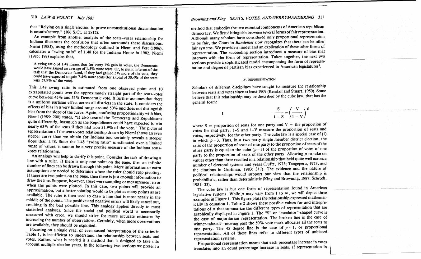
The cube law is but one form of representation found in American legislative systems. While p may vary from 1 to oo, we will depict three examples in Figure 1. This figure plots the relationship expressed mathemat- ically in equation 1. Table 2 shows these possible values for and interpre- tations of p that summarize the different types of representation that are graphically displayed in Figure 1. The "S" or "escalator"-shaped curve is the case of majoritarian representation. The broken line is the case of winner-take-all-moving past the 50% vote mark allocates all the seats to one party. The 45 degree line is the case of p = 1, or proportional representation. All of these lines refer to different types of unbiased representation systems.

Proportional representation means that each percentage increase in votes translates into an equal percentage increase in seats. If representation in r

312 LA W & POLICY July 1987

Figure 1. Forms of Unbiased Representation

Proportion Democratic Votes

NOTE: Lines are drawn based on Equation 1.

Table 2. Representation Coefficient Values

Coefficient Representation type

p = a , winner-take-all w > p > l majoritarian p = 1 proportional

American legislatures were allocated according to a strictly proportional rule, one could expect a party to win 55% of the seats by winning 55% of the vote, for example. Many have mistakenly used proportionality as the standard to evaluate fairness. Dixon (1971: 13) characterizes this dilemma: "A paradox of the one man, one vote, revolution is that we now perceive our goal to be something approaching a proportional result, in terms of group access to the legislative process, while retaining the district method of election." The Bandemer majority spoke clearly on this point: "Our cases, however, clearly foreclose any claim that the Constitution requires proportional representation or that legislatures in reapportioning must draw district lines to come as near as possible to allocating seats to the contending parties in proportion to what their anticipated statewide vote

Browning and King SEA TS, VOTES, AND GERRYMANDERING 3 13

will be. Whitcomb v. Chavis, 402 U.S., at 153, 146, 160; White v. Regester, 412 U.S., at 765-766" (106 S.Ct at 2809).

A second type of representation depicted in Figure 1 is winner-take-all, where p in equation 1 is equal to infinity. Here 50% plus one vote results in 100% of the seats. As p approaches infinity the party with less than 50% plus one vote gets no seats and the "winner takes all." When there is only one district and one member, we use winner-take-all. Small states with one representative, such as Wyoming and Alaska, are winner-take-all states. The election of the president is a case of winner-take-all representation. In the United States, we use winner-take-all representation on a district and state basis for the House of Representatives and the Senate respectively. For state legislatures, the use of large multi-member districts are effectively winner-take-all. For example, in the late 1960s fifteen members were elected to the Indiana House at-large from Marion County (Indianapolis). This point was noted in Whitcomb v. Chavis (402 U.S. 124 (1971)) in which the country- wide multi-member districts were upheld by the Supreme Court.

A striking but typical example of the importance of party affiliation and the "winner take all" effect is shown by the 1964 House of Representatives election. [Figures omitted here.] Though nearly 300,000 Marion County voters cast nearly 4% million votes for the House, the high and low candidates within each party varied by only about a thousand votes. And, as these figures show, the Republicans lost every seat though they received 48.69% of the vote. Plaintiffs' Exhibit 10. Whitcomb v. Chavis (402 U.S. 124 at 133-34 n. 11).

The final form of representation displayed in Figure 1 is majoritarian. Represented by the steep "escalator"-shaped curve, where p = 3, it reflects an important principle of the United States two-party, democratic system. It helps majorities form, yet protects the minority party. Once a party approaches the 50% point, it easily gains additional seats helping it form a governing, legislative majority. Others have termed this the "balloon effect" (See Backstrom et al., 1978: 1134 and Grofman, 1985a: 159; see Niemi, 1985). It is difficult, however, for one party to gain all the seats and deprive the minority of representation. This can be seen in how the curve flattens out as it moves towards the ends of the distribution. As p increases from one to a, the seats-votes curve steepens near the middle and flattens out near the ends, indicating that the party is winning more seats than its proportionate share of votes in the middle range and less seats towards the ends.

Others (Tufte, 1973; Niemi and Fett, 1986) have represented this majoritarian curve as a straight line since most of the points fall in the central portion that does appear relatively straight. This simplification has also been justified because the linear form is easier to comprehend than the non-linear, cube form. However, the linear form neglects the important information we gain from observing the flatness at the extremes and the variation in state electoral systems that gives rise to a variety of shapes and values of p. Any effort to interpret seats-votes relationships as indicators of

314 LAW & POLICY July 1987

political gerrymandering must consider the historical nature of the particular state in question. As Justice O'Connor wrote in her concurring opinion in Bandemer, "Redistricting itself represents a middle ground between winner- take-all statewide elections and proportional representation for political parties" (106 S.Ct. at 2824). Our model estimates redistricting in this middle ground rather than suggesting as O'Connor feared "that the greater the departure from proportionality, the more suspect an apportionment plan becomes." (106 S.Ct. at 2824).

All of these three types are fair representation because of partisan symmetry; that is, they treat each party equally. The seats-votes curves of Figure 1 are symmetric and thus evidence no bias. The "escalator" curve is symmetrical about 50% indicating that each party is treated the same and that parties are assisted in their effort to achieve a majority as the percentage of their votes nears 50%. While the "balloon" effect helps majorities form and protects minorities, it is fair because the other party would experience the same effect if it were to achieve a majority.

Others have described this effect as bias. See, for example, Backstrom et al.'s (1978: 1134) comment that "The balloon effect has been demonstrated empirically. Because the percentage of districts won by the dominant party tends to be higher than its percentage of the statewide popular vote, Dixon 11968: 50-541 has observed that single-member districting creates at least a mild bias in favor of the dominant party." Niemi (1985) also referred to the steepness of the "escalator" curve as indicating bias. Even the district court in Bandemer referred to the single seats-votes statistic as evidence of "the suspicion of this kind of built-in bias." (603 F. Supp. at 1486). Our objections to these statements is, in part, definitional. The word "bias" has been used to mean very different things. We use the term "bias" to indicate deviations from partisan symmetry. Nevertheless, the concepts of invidious partisan bias and different fair systems of democratic representation remain confused in court opinions and scholarly analyses.

V. BIAS

h a model we develop elsewhere (King and Browning, 1987) we add a parameter to the general form of the seats-votes relationship in equation 1. This parameter, P, Equation 2 is included to allow for bias defined as partisan asymmetry. Its effect is to cause the lines in Figure 1 to shift to the right or to the left. If the lines do not pass through the intersection of 50% votes and 50% seats, the form of representation is biased. A party could thus achieve a lesiglative majority by gaining less than 50% of the votes. The effect of bias on the basic forms of representation are shown in Figures 2 and 3.

Browning and King SEA TS, VOTES, AND GERR YMANDERING

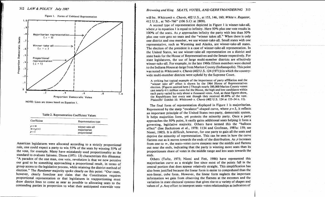
Figure 2. Bias and Proportional Representation

0 . 5 . o

Proportion Democratic Votes

NOTES: Lines are drawn based on Equation 2

Representation is the steepness or flatness of the curve, whereas bias measures the extent to which the seats-votes relationship favors one party or the other. Figures 2 and 3 show that the effect of bias varies depending on where one is on the curve. With proportional representation (in Figure 2), one can readily see that difference between the curves varies as one moves away from 50%. The lower curve, where ln(P)= - 1, is biased toward the Republicans; the upper curve, where In@) = 1, is biased toward the Democrats. On the lower curve, the Democrats need almost 75% of the vote to win a legislative majority. On the upper curve, they need only 27%.

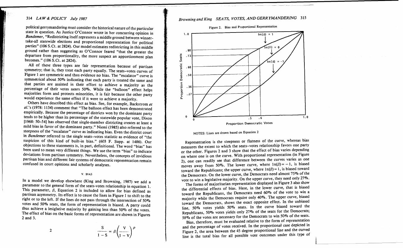
The forms of majoritarian representation displayed in Figure 3 also show the differential effects of bias. Here, in the lower curve, that is biased toward the Republicans, the Democrats need 60% of the vote to win a majority while the Democrats require only 40%. The upper curve, biased toward the Democrats, shows the exact opposite effect. In the unbiased line, 50% votes yields 50% seats. In the curve biased toward the Republicans, 50% votes yields only 27% of the seats for the Democrats; 58% of the votes are necessary for the Democrats to win 50% of the seats.

Bias, therefore, must be evaluated relative to the form of representation and the percentage of votes received. In the proportional case depicted in Figure 2, the area between the 45 degree proportional line and the curved line is the total bias for all possible vote outcomes under this type of

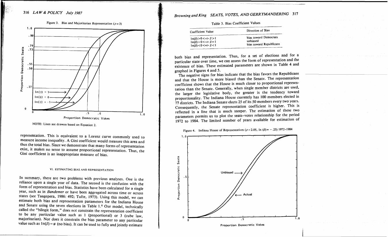
3 16 LA W & POLICY July 1987

Figure 3. Bias and Majoritarian Representation ( p = 3)

Proportion Democratic Votes

NOTE: Lines are drawnn based on Equation 2.

represetltation. This is equivalent to a Lorenz curve commonly used to measure income inequality. A Gini coefficient would measure this area and thus the total bias. Since we demonstrate that many forms of representation exist, it makes no sense to assume proportional representation. Thus, the Gini coefficient is an inappropriate measure of bias.

V1. ESTIMATING BIAS AND REPRESENTATION

In summary, there are two problems with previous analyses. One is the reliance upon a single year of data. The second is the confusion with the form of representation and bias. Statistics have been calculated for a single year, such as in Bandemer or have been aggregated across time or across states (see Taagepera, 1986: 492; Tufte, 1973). Using this model, we can estimate both bias and representation parameters for the Indiana House and Senate using the seven elections in Table Our model, technically called the "bilogit form," does not constrain the representation coefficient to be any particular value such as 1 (proportional) or 3 (cube law, majoritarian). Nor does it constrain the bias parameter to any particular value such as ln(P) = 0 (no bias). It can be used to fully and jointly estimate

Browning and King SEA TS, VOTES, AND GERR YMANDERZNG 3 17

Table 3. Bias Coefficient Values

Coefficient Value Direction of Bias

In@) >O <=> 6 > 1 bias toward Democrats ln(D)=O<=> P= 1 unbiased ln(B)<O<=> P<1 bias toward Republicans

both bias and representation. Thus, for a set of elections and for a particular state over time, we can assess the form of representation and the existence of bias. These estimated parameters are shown in Table 4 and graphed in Figures 4 and 5.

The negative signs for bias indicate that the bias favors the Republicans and that the House is more biased than the Senate. The representation coefficient shows that the House is much closer to proportional represen- tation than the Senate. Generally, when single member districts are used, the larger the legislative body, the greater is the tendency toward proportionality. The Indiana House currently has 100 members elected in 77 districts. The Indiana Senate elects 25 of its 50 members every two years. Consequently, the Senate representation coefficient is higher. This is reflected in a line that is much steeper. The estimation of these two parameters permits us to plot the seats-votes relationship for the period 1972 to 1984. The limited number of years available for estimation of

Figure 4. Indiana House of Representatives ( p = 2.05, In (P) = - .25) 1972-1984

Proportion Democratic Votes

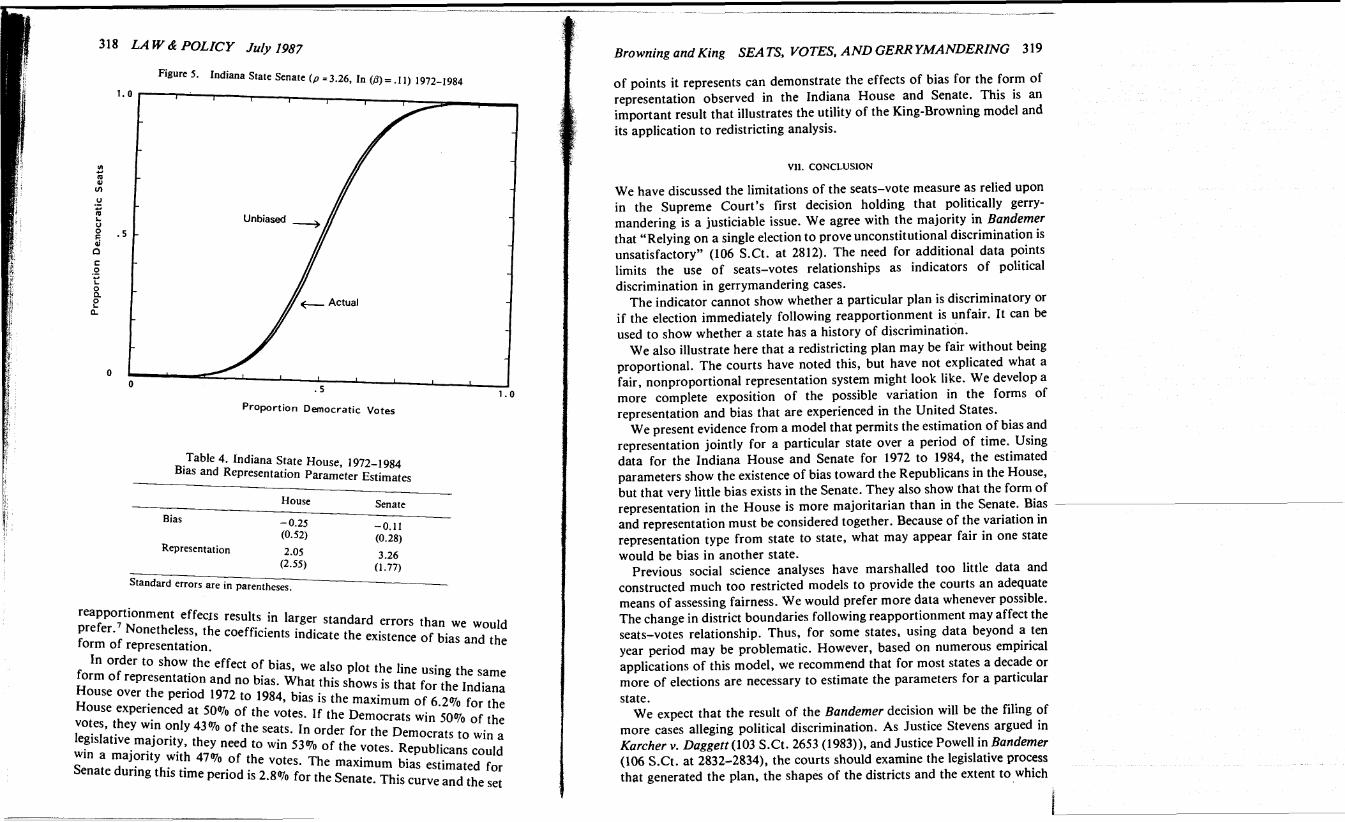
3 18 LA W & POLICY July 1987

Proportion Democratic Votes

Table 4. Indiana State House, 1972-1 984 Bias and Representation Parameter Estimates

- House Senate

Bias - 0.25 -0.11 (0.52) (0.28)

Representation 2.05 3.26

(2.55) (1.77)

Standard errors are in parentheses.

reapportionment effecls results in larger standard errors than we would prefer.' Nonetheless, the coefficients indicate the existence of bias and the form of representation.

In order to show the effect of bias, we also plot the line using the same form of representation and no bias. What this shows is that for the Indiana House over the period 1972 to 1984, bias is the maximum of 6.2% for the House experienced at 50% of the votes. If the Democrats win 50% of the votes, they win only 43% of the seats. In order for the Democrats to win a legislative majority, they need to win 53% of the votes. Republicans could win a majority with 47% of the votes. The maximum bias estimated for Senate during this time period is 2.8% for the Senate. This curve and the set

Browning and King SEATS, VOTES, AND GERR YMANDERING 3 19

of points it represents can demonstrate the effects of bias for the form of representation observed in the Indiana House and Senate. This is an important result that illustrates the utility of the King-Browning model and its application to redistricting analysis.

V11. CONCLUSION

We have discussed the limitations of the seats-vote measure as relied upon in the Supreme Court's first decision holding that politically gerry- mandering is a justiciable issue. We agree with the majority in Bandemer that "Relying on a single election to prove unconstitutional discrimination is unsatisfactory" (106 S.Ct. at 2812). The need for additional data points limits the use of seats-votes relationships as indicators of political discrimination in gerrymandering cases.

The indicator cannot show whether a particular plan is discriminatory or if the election immediately following reapportionment is unfair. It can be used to show whether a state has a history of discrimination.

We also illustrate here that a redistricting plan may be fair without being proportional. The courts have noted this, but have not explicated what a fair, nonproportional representation system might look like. We develop a more complete exposition of the possible variation in the forms of representation and bias that are experienced in the United States.

We present evidence from a model that permits the estimation of bias and representation jointly for a particular state over a period of time. Using data for the Indiana House and Senate for 1972 to 1984, the estimated parameters show the existence of bias toward the Republicans in the House, but that very little bias exists in the Senate. They also show that the form of representation in the House is more majoritarian than in the Senate. Bias and representation must be considered together. Because of the variation in representation type from state to state, what may appear fair in one state would be bias in another state.

Previous social science analyses have marshalled too little data and constructed much too restricted models to provide the courts an adequate means of assessing fairness. We would prefer more data whenever possible. The change in district boundaries following reapportionment may affect the seats-votes relationship. Thus, for some states, using data beyond a ten year period may be problematic. However, based on numerous empirical applications of this model, we recommend that for most states a decade or more of elections are necessary to estimate the parameters for a particular state.

We expect that the result of the Bandemer decision will be the filing of more cases alleging political discrimination. As Justice Stevens argued in Karcher v. Daggett (103 S.Ct. 2653 (1983)), and Justice Powell in Bandemer (106 S.Ct. at 2832-2834), the courts should examine the legislative process that generated the plan, the shapes of the districts and the extent to which

320 LA W & POLICY July I987

they respect existing political subdivisions, and the extent t o which the mapmakers were motivated only by partisan interests. The model we present and the analysis of the statistical data for Indiana should not be viewed as a single indicator of political discrimination, but ought to be interpreted by the courts as part of the totality of evidence needed to prove unconstitutional gerrymandering. As Justice Powell wrote in Bandemer (106 S.Ct. a t 2826): "Because the plurality ignores such factors and fails to enunciate standards by which t o determine whether a legislature has enacted an unconstitutional gerrymandering, I dissent." Future research, such as ours explicating the theoretical and empirical forms of fair representation, can help establish these standards.

ROBERT x BROWNING is Associate Professor of Political Science at Purdue University. He is the author of Politics and Social Welfare Policy in the United States and several articles on Indiana politics. He has served as a redistricting consultant to the Indiana House following the district court Bandemer decision, but was not involved in the preparation of that case.

GARY KING is Associate Professor of Government at Harvard University. He has co- authored The Elusive Executive: Discovering Statistical Patterns in the Presidency and has also written several articles on American politics and on quantitative methods.

NOTES

1. Both the district court decision and the Supreme Court decision will be referred to as the Bandemer case.

2. The Bandemer case was brought by Indiana Democrats challenging the redistricting of the Indiana Statehouse by the majority Republicans following the 1980 census and prior to the 1982 election. On December 13, 1984 the district court ruled 2-1 in favor of the Democrats (see 603 F. Supp. 1479 (S.D. Ind. 1984)). The Republicans appealed to the Supreme Court which ruled in favor of the Republicans June 30, 1986 (David v. Bandemer, 106 S.Ct. 2797 (1986)). Con- solidated with the district court case was another lawsuit filed by the Indiana NAACP charging unconstitutional dilution of minority voting strength. The district court rejected this claim noting "the voting efficacy of the NAACP plaintiffs was impinged upon because of their politics and not because of their race." 603 F. Supp., at 1489-1490.

3. The auditor was the only Democratic candidate to win a statewide contest with 51.1% of the vote. The Democratic vote for clerk was 49.2%. Averaging these two races evens out advantages which these individual candidates experienced in their home counties. It is also close to the Democratic statewide vote for secretary of state (48.1 %).

4. In the normal vote analysis, we presume "winner-take-all" for House multi- member districts. That is, the party with the "normal" vote majority wins all of the seats in the district. In 1982, four of the nine double member districts elected representatives of both parties. Six of the seven triple member districts elected all Republicans; one elected all Democrats. The Indiana Senate contains only single member districts.

5. It is also important to retain comparability across observations. For example, aggregating data across states appears to make little sense. Reapportionment is

Browning and King SEA TS, VOTES, AND GERRYMANDERING 321

conducted separately by each state legislature. The number of representatives allocated to a state, the degree of party competition within the state, the geographical distribution of votes within the state, the number of uncontested seats, and the number of incumbents can all influence the seat-votes ratio within a state. Combining states can only confound the analysis.

6. These seven elections encompass two reapportionment decades. This grouping is necessary into order to obtain a sufficient number of data points for the estimation of blas and representation. Since the 1970 and 1980 reapportionments in Indiana were conducted by Republican majorities, the assumption that the plans were generated by similar underlying processes is a reasonable one. Extending the period to include the reapportionments of the 1960s would compromise this assumption because of changing nature of redistricting and party margins between 1963 and 1970 (see Hardy et al., 1981).

7. In an estimation for U.S. Congressional elections reported in King and Browning (1987) where eighteen elections are used rather than the seven used here, much smaller standard errors are obtained in many of the states. An additional, second stage analysis in that paper also helps to demonstrate the validity of our estimates.

REFERENCES

BACKSTROM. c.. L. ROBINS and s. ELLER (1978) "Issues in Gerrymandering: An Exploratory Measure of Partisan Gerrymandering Applied to Minnesota," Minnesota Law Review 62: 1121-1159.

CAMPBELL. J. E. (1986) "Presidential Coattails and Midterm Losses in State Legislative Elections," American Political Science Review 80: 45-64.

DIXON. R. G.. JR. (1971) "The Court, the People, and 'One Man, One Vote'," in Nelson W. Polsby (ed.) Reapportionment in the 1970s. Berkeley: University of California.

GROFMAN. B. N., A. LIJPHART, R. B. MCKAY, and H. A. SCARROW (eds.) (1982) Representation and Redistricting Issues. Lexington, Mass: D.C. Heath.

GROFMAN, B. N. (1983) "Measures of Bias and Proportionality in Seats-Votes Relation- ships," Political Methodology 10: 295-327.

GROFMAN. B. N. (1985a) "Criteria for Districting: A Social Science Perspective," UCLA Law Review 33: 77-184.

GROFMAN. B. N. (1985b) "Political Gerrymandering: Badham v. Eu, Political Science Goes to Court," PS 538-581.

HARDY. L., A. HESLOP, and s. ANDERSON (eds.) (1981) Reapportionment Politics. Beverly Hills: Sage.

KENDALL, M. G.. and A. STUART (1950) "The Law of Cubic Proportion in Election Results," British Journal of Sociology 1: 183-97.

KING. G and R. x. BROWNING (1987) "Democratic Representation and Partisan Bias in Congressional Elections," American Political Science Review, 81 (December).

NIEMI. R. G. (1985) "The Relationship between Votes and Seats: The Ultimate Question in Political Gerrymandering," UCLA Law Review 33: 185-212.

NIEMI, R. G. and P. F E ~ T (1986) "The Swing Ratio: An Explanation and an Assessment," Legislative Studies Quarterly XI, 1 (February): 75-90.

SCHRODT. P. A. (1981) "A Statistical Study of the Cube Law in Five Electoral Systems," Political Methodology 7: 3 1-54.

TAAGEPERA, R. (1973) "Seats and Votes: A Generalization of the Cube Law of Elections," Social Science Research 2: 257-75.

322 LA W & POLICY July 1987

TAAGEPERA. R. (1986) "Reformulating the Cube Law for Proportional Representation Elections," American Political Science Review 80: 489-504.

NFTE. E. R. (1973) "The Relationship Between Seats and Votes in Two-Party Systems, " American Political Science Review 67: 540-554.

COURT CASES

Badham v. Eu., No. C-83-1126 (N.D. Cal. 1984). Bandemer v. Davis. 603 F. Supp. 1479 (S.D. Ind. 1984). Davis v. Bandemer. 106 S.Ct. 2797 (1986). Karcher v. Daggett. 462 U.S. 725 (1983). Whitcomb v. Chavis. 402 U.S. 124 (1971). White v. Regester. 412 U.S. 755 (1973).

An Enforcement Taxonomy of Regulatory Agencies

JOHN BRAITHWAITE, JOHN WALKER and PETER GRABOSKY*

A variety of multivariate techniques were used to develop a taxonomy of regulatory agencies from the first comprehensive study of the dkparate enforcement strategies employed by business regulatory agencies in one country. Seven types of agencies were identified: Conciliators, Benign Big Guns, Diagnostic Znspectorates, Detached Token Enforcers, Detached Modest En forcers, Token En forcers and Modest En forcers. Agencies were distinguished primarily according to their orientation to enforcement versus persuasion, according to their commitment to detached (or arms length) com- mand and control regulation versus cooperative fostering of self-regulation, and according to their attachment to universalistic rulebook regulation versus particularistic regulation. Nevertheless, it is not unreasonable to view regulatory agencies as lying on a single continuum from particularistic non- enforcers who engage in cooperative fostering of self-regulation to rulebook enforcers whose policy is detached command and control. Thk approximates the suggestions of Hawkins and Reiss for distinguishing regulatory agencies according to a 'kanctioning/deterrence" versus "compliance" dimension. The predominant regulatory style in Australia, however, is distant from both poles, being a perfunctory regulatory approach which is neither distinctively diagnostic and educative nor litigiously "going by the book"; rather it amounts to "going through the motions". The typology ako partially conforms to Black's categorisation of social control as penal, therapeutic, conciliatory and compensatory.

I. INTRODUCTION

Despite the growing interest in institutions and processes of business regulation throughout the western world, there has yet to be a systematic, empirically based typology of regulatory agencies.

Thus far, most efforts to characterise regulatory agencies have tended to emphasise the specification of ideal types. These lie at either end of a continuum of formality suggested by the more general work of Black (1976). The more formal style of regulation, for which Reiss (1984) uses the term "deterrence" and Hawkins (1984) the term "sanctioning", is based essentially upon a penal response to a regulatory violation. The general concern is the application of punishment for corporate misconduct, for retributive and deterrent purposes. A harmful or potentially harmful act in

*We wish to thank Debra Rickwood. Yvonne Pittelkow, Terry Speed, Frank Jones. Bruce Biddle and Jonathan Kelley for assistance and helpful suggestions on the analyses in this paper.

LAW & POLICY, Vol. 9. No. 3, July 1987 O 1987 Basil Blackwell ISSN 0265-8240 $3.00