Parallel Strategies for Local Biological Sequence Alignment in a Cluster of Workstations

J. Parallel Distrib. Comput. 67 (2007) 170–185www.elsevier.com/locate/jpdc

Parallel strategies for the local biological sequence alignment in a cluster ofworkstations

Azzedine Boukerchea, Alba Cristina Magalhaes Alves de Melob,∗, Mauricio Ayala-Rincónc,Maria Emilia Machado Telles Walterb

aSchool of Information Technology and Engineering, University of Ottawa, CanadabDepartamento de Ciência da Computação, Universidade de Brasília, Brazil

cDepartamento de Matemática, Universidade de Brasília, Brazil

Received 17 September 2005; received in revised form 24 September 2006; accepted 2 November 2006

Abstract

Recently, many organisms have had their DNA entirely sequenced. This reality presents the need for comparing long DNA sequences,which is a challenging task due to its high demands for computational power and memory. Sequence comparison is a basic operation in DNAsequencing projects, and most sequence comparison methods currently in use are based on heuristics, which are faster but offer no guarantees ofproducing the best alignments possible. In order to alleviate this problem, Smith–Waterman proposed an algorithm. This algorithm obtains thebest local alignments but at the expense of very high computing power and huge memory requirements. In this article, we present and evaluateour experiments involving three strategies to run the Smith–Waterman algorithm in a cluster of workstations using a Distributed Shared MemorySystem. Our results on an eight-machine cluster presented very good speed-up and indicate that impressive improvements can be achieveddepending on the strategy used. In addition, we present a number of theoretical remarks concerning how to reduce the amount of memory used.© 2006 Elsevier Inc. All rights reserved.

Keywords: Cluster computing; Sequence alignment; Analysis of parallel algorithms

1. Introduction

Biological sequence comparison is one of the most impor-tant problems in computational biology given the number anddiversity of the sequences and the frequency with which theymust be solved on a daily basis all over the world [20]. Se-quence comparison is in fact a problem of finding an approx-imate pattern match between two sequences; this can possiblyinvolve the introduction of spaces (gaps).

The most important types of sequence alignment problemsare global and local. To solve a global alignment problem isto find the best match between the entire sequences. Localalignment algorithms must find the best match (or matches)

∗ Corresponding author.E-mail addresses: [email protected] (A. Boukerche),

[email protected] (A.C.M.A. de Melo),[email protected] (M. Ayala-Rincón), [email protected] (M.E.M.T. Walter).

0743-7315/$ - see front matter © 2006 Elsevier Inc. All rights reserved.doi:10.1016/j.jpdc.2006.11.001

between parts of the sequences. In this article we will deal forthe most part with local alignments.

Smith and Waterman [21] proposed an algorithm (SW) basedon dynamic programming to solve the local alignment problem.It is an exact algorithm that finds the best local alignmentsbetween two genomic sequences of size n in quadratic time andspace complexity O(n2). In genome projects, the size of thesequences to be compared is constantly increasing; thus, usingan O(n2) solution remains expensive. For this reason, heuristicswere proposed to reduce time complexity to O(n). BLAST [2]and FASTA [18] are examples of widely used heuristics thatcompute local alignments.

SW is the most sensitive method of solving the problem butis also the slowest one in terms of similar searches betweensequences. One obvious improvement is the use of parallelprocessing to speed-up SW computations. However, even inthis case the quadratic space complexity remains a problem.Techniques must therefore be used to reduce it.

Martins [14] and MASPAR [6] proposed techniques to runthe SW algorithm in, respectively, a Beowulf machine with

http://www.elsevier.com/locate/jpdc

mailto:[email protected]




A. Boukerche et al. / J. Parallel Distrib. Comput. 67 (2007) 170–185 171

128 processors and a massively parallel computer system with16,384 processors. Although the results obtained in both caseswere good, the cost of such machines makes this an expensiveapproach. Decypher [5] is a dedicated hardware based on FP-GAs that implements the SW algorithm. It is also an expensiveapproach.

In this article, we propose and evaluate three parallel strate-gies to implement the SW algorithm in a cluster of worksta-tions that use commodity hardware and a Unix-like operatingsystem. The first two strategies (heuristic and heuristic-block)are approximate since they use heuristics to reduce the spacecomplexity. The last strategy (pre-process) is an exact one thatstores intermediate results in a disk. In addition, we propose amodification to the original SW algorithm, which runs in spacecomplexity O(n + n′2) where n′ is the maximum length of alocal alignment between sequences s and t of size n.

The results obtained in an eight-machine cluster with largesequence sizes show good speed-ups when compared to the se-quential algorithm. Moreover, each of the proposed techniquesprovides significant improvement over the former strategy. Forinstance, when comparing 50 kBP (kilo-base pair) sequencesusing eight processors, heuristic-block provides a reduction of304% over the execution time of the heuristic strategy on thesame platform. Furthermore, for 80 kBP sequences, the pre-process strategy runs approximately 12 times faster than theheuristic one.

This paper is organized as follows. Section 2 briefly de-scribes the local sequence alignment problem and the SW al-gorithm used to solve it. Section 3 presents the concept of Dis-tributed Shared Memory (DSM) and introduces JIAJIA, theDSM system that was used in our implementations. Section 4describes the two heuristic strategies that were used to imple-ment the modified SW algorithm in a parallel platform andpresents some experimental results. Section 5 describes the im-provements proposed to implement the original SW algorithmin a parallel platform and discusses certain experimental re-sults. Section 6 points out possible improvements to the SWalgorithm that reduce its memory requirements, thereby pro-ducing exact answers. Finally, Section 7 concludes the paperand presents future work.

2. Smith–Waterman’s algorithm for local sequencealignment

In order to compare two sequences, we must find the bestalignment between them, which is to place one sequence abovethe other, thereby making clear the correspondence betweensimilar characters or substrings of the sequences [20]. Duringan alignment, spaces are inserted in arbitrary locations alongthe sequences so that all sequences are of the same size.

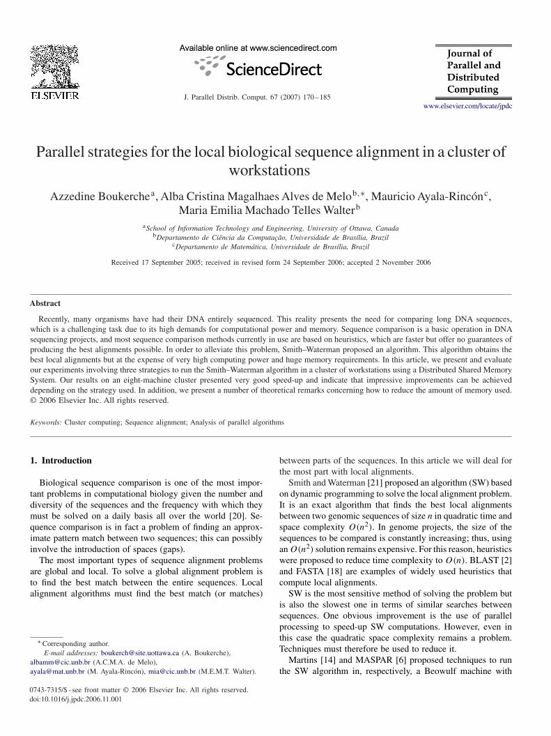
Given an alignment between two sequences s and t, a scoreis associated as follows. For each column, we associate, forinstance, +1 if the two characters are identical, −1 if the char-acters are different and −2 if one of them is a space. Thescore is the sum of the values computed for each column. Themaximum score is the similarity between the two sequencesand is denoted by sim(s, t). In general, there are many align-

Fig. 1. Alignment between s = GACGGATTAG and t = GATCGGAATAG.

AC

C...

......

......

.....C

TTA

AG

GC

......

......

....G

GC

AA

......

...G

G

ATG...................CTTTAGGG...............GGCAT.........AT

similarityregions

Fig. 2. Local alignment of two 400 kBP sequences, which produced twosimilar regions.

ments with a maximum score. Fig. 1 shows the alignment ofsequences s and t with the score for each column. In this case,there are nine columns with identical characters, one columnwith a distinct character, and one column with a space, givinga total score of 6.

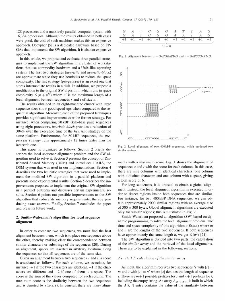
For long sequences, it is unusual to obtain a global align-ment. Instead, the local alignment algorithm is executed in or-der to detect regions inside both sequences that are similar.For instance, for two 400 kBP DNA sequences, we can ob-tain approximately 2000 similar regions with an average sizeof 300 × 300 bytes. Global alignment algorithms are executedonly for similar regions; this is illustrated in Fig. 2.

Smith–Waterman proposed an algorithm (SW) based on dy-namic programming to solve the local alignment problem. Thetime and space complexity of this algorithm is 0(mn) where mand n are the lengths of the two sequences. If both sequenceshave approximately the same length n, we get O(n2) [21].

The SW algorithm is divided into two parts: the calculationof the similar array and the retrieval of the local alignments.These are to be explained in the following sections.

2.1. Part 1: calculation of the similar array

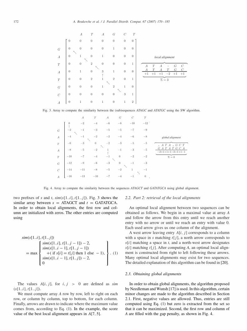
As input, the algorithm receives two sequences ‘s with |s| =m and t with |t | = n’ where |s| denotes the length of sequences. There are m+1 possible prefixes for s and n+1 prefixes for t,including the empty string. An array Am+1,n+1 is built in whichthe A[i, j ] entry contains the value of the similarity between

172 A. Boukerche et al. / J. Parallel Distrib. Comput. 67 (2007) 170–185

Fig. 3. Array to compute the similarity between the (sub)sequences ATAGC and ATATGC using the SW algorithm.

Fig. 4. Array to compute the similarity between the sequences ATAGCT and GATATGCA using global alignment.

two prefixes of s and t, sim(s[1..i], t[1..j ]). Fig. 3 shows thesimilar array between s = ATAGCT and t = GATATGCA.In order to obtain local alignments, the first row and col-umn are initialized with zeros. The other entries are computedusing

sim(s[1..i], t[1..j ])

= max

⎧⎪⎪⎪⎪⎨⎪⎪⎪⎪⎩

sim(s[1..i], t[1..j − 1]) − 2,

sim(s[1..i − 1], t[1..j − 1])+( if s[i] = t[j ] then 1 else − 1),

sim(s[1..i − 1], t[1..j ]) − 2,

0

⎫⎪⎪⎪⎪⎬⎪⎪⎪⎪⎭

. (1)

The values A[i, j ], for i, j > 0 are defined as sim(s[1..i], t[1..j ]).

We must compute array A row by row, left to right on eachrow, or column by column, top to bottom, for each column.Finally, arrows are drawn to indicate where the maximum valuecomes from, according to Eq. (1). In the example, the scorevalue of the best local alignment appears in A[7, 5].

2.2. Part 2: retrieval of the local alignments

An optimal local alignment between two sequences can beobtained as follows. We begin in a maximal value at array Aand follow the arrow from this entry until we reach anotherentry with no arrow or until we reach an entry with value 0.Each used arrow gives us one column of the alignment.

A west arrow leaving entry A[i, j ] corresponds to a columnwith a space in s matching t[j ], a north arrow corresponds tos[i] matching a space in t, and a north-west arrow designatess[i] matching t[j ]. After computing A, an optimal local align-ment is constructed from right to left following these arrows.Many optimal local alignments may exist for two sequences.The detailed explanation of this algorithm can be found in [20].

2.3. Obtaining global alignments

In order to obtain global alignments, the algorithm proposedby Needleman and Wunsh [17] is used. In this algorithm, certainminor changes are made to the algorithm described in Section2.1. First, negative values are allowed. Thus, entries are stillcomputed using Eq. (1) but zero is extracted from the set sothat it can be maximized. Second, the first row and column ofA are filled with the gap penalty, as shown in Fig. 4.


3. Distributed shared memory

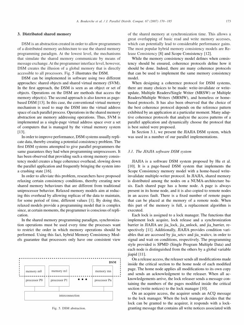
DSM is an abstraction created in order to allow programmersof a distributed memory architecture to use the shared memoryprogramming paradigm. At the lowest level, the mechanismsthat simulate the shared memory communicate by means ofmessage exchange. At the programmer interface level, however,DSM creates the illusion of a global memory that is directlyaccessible to all processors. Fig. 5 illustrates the DSM.

DSM can be implemented in software using two differentapproaches: shared objects and shared virtual memory (SVM).In the first approach, the DSM is seen as an object or set ofobjects. Operations on the DSM are methods that access thememory object(s). The second approach is also known as page-based DSM [13]. In this case, the conventional virtual memorymechanism is used to map the DSM into the virtual addressspace of each parallel process. Operations in the shared memoryabstraction are memory addressing operations. Thus, SVM isimplemented as a single-page virtual address space over a setof computers that is managed by the virtual memory system[13].

In order to improve performance, DSM systems usually repli-cate data, thereby creating a potential consistency problem. Thefirst DSM systems attempted to give parallel programmers thesame guarantees they had when programming uniprocessors. Ithas been observed that providing such a strong memory consis-tency model creates a huge coherence overhead, slowing downthe parallel application and frequently bringing the system intoa crashing state [16].

In order to alleviate this problem, researchers have proposedrelaxing certain consistency conditions, thereby creating newshared memory behaviours that are different from traditionaluniprocessor behavior. Relaxed memory models aim at reduc-ing this overhead by allowing replicas of the data to maintain,for some period of time, different values [1]. By doing this,relaxed models provide a programming model that is complexsince, at certain moments, the programmer is conscious of repli-cation.

In the shared memory programming paradigm, synchroniza-tion operations must be used every time the processes wantto restrict the order in which memory operations should beperformed. Using this fact, hybrid Memory Consistency Mod-els guarantee that processors only have one consistent view

memory m0

processor P0

interconnection

DSM

memory mnmemory m1

processor Pnprocessor P1

Fig. 5. DSM abstraction.

of the shared memory at synchronization time. This allows agreat overlapping of basic read and write memory accesses,which can potentially lead to considerable performance gains.The most popular hybrid memory consistency models are Re-lease Consistency [8] and Scope Consistency [12].

While the memory consistency model defines when consis-tency should be ensured, coherence protocols define how itshould be done. Indeed, there are many coherence protocolsthat can be used to implement the same memory consistencymodel.

When designing a coherence protocol for DSM systems,there are many choices to be made: write-invalidate or write-update, Multiple Readers/Single Writer (MRSW) or MultipleReaders/Multiple Writers (MRMW), and homeless or home-based protocols. It has also been observed that the choice ofthe best coherence protocol depends on the reference patternexhibited by an application at a particular moment. Many adap-tive coherence protocols that analyze the access patterns of aparallel application and dynamically choose the protocol thatis best suited were proposed.

In Section 3.1, we present the JIAJIA DSM system, whichwas used in a number of our parallel implementations.

3.1. The JIAJIA software DSM system

JIAJIA is a software DSM system proposed by Hu et al.[10]. It is a page-based DSM system that implements theScope Consistency memory model with a home-based write-invalidate multiple-writer protocol. In JIAJIA, shared memoryis distributed among the nodes on a NUMA-architecture ba-sis. Each shared page has a home node. A page is alwayspresent in its home node, and it is also copied to remote nodesin an access fault. There is a fixed number of remote pagesthat can be placed at the memory of a remote node. Whenthis part of the memory is full, a replacement algorithm isexecuted.

Each lock is assigned to a lock manager. The functions thatimplement lock acquire, lock release and a synchronizationbarrier in JIAJIA are jia_lock, jia_unlock, and jia_barrier, re-spectively [11]. Additionally, JIAJIA provides condition vari-ables that are accessed by jia_setcv and jia_waitcv, in order tosignal and wait on conditions, respectively. The programmingstyle provided is SPMD (Single Program Multiple Data) andeach node is distinguished from the others by a global variablejiapid [11].

On a release access, the releaser sends all modifications madeinside the critical section to the home node of each modifiedpage. The home node applies all modifications to its own copyand sends an acknowledgment to the releaser. When all ac-knowledgements arrive, the lock releaser sends a message con-taining the numbers of the pages modified inside the criticalsection (write notices) to the lock manager [10].

On an acquire access, the acquirer sends an ACQ messageto the lock manager. When the lock manager decides that thelock can be granted to the acquirer, it responds with a lock-granting message that contains all write notices associated with


Node 1Node 0

(barrier manager)

Node 2

sends diffs tohome nodes

applies diffsapplies diffs

DIFF DIFF

generates diffsand write notices

DIFFGRANT DIFFGRANT

sends barriermessage

write notices

BARR

BARRGRANT

write notices

invalidatesremote pages

sets pagesstate to R/O

clearswrite notices

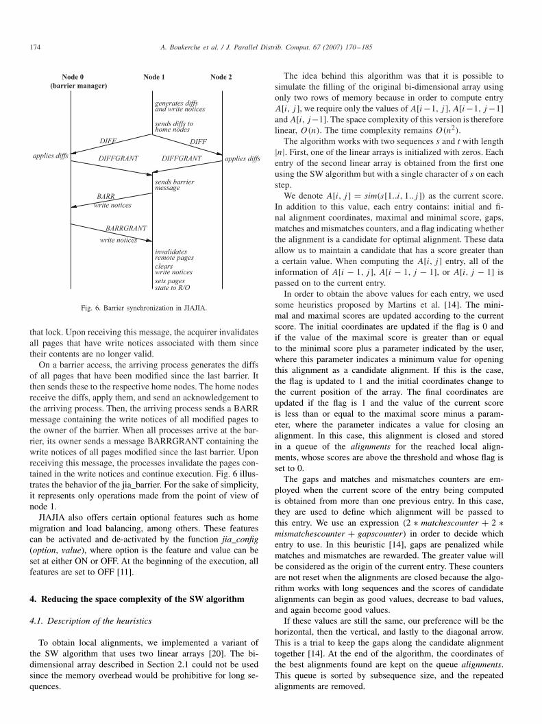
Fig. 6. Barrier synchronization in JIAJIA.

that lock. Upon receiving this message, the acquirer invalidatesall pages that have write notices associated with them sincetheir contents are no longer valid.

On a barrier access, the arriving process generates the diffsof all pages that have been modified since the last barrier. Itthen sends these to the respective home nodes. The home nodesreceive the diffs, apply them, and send an acknowledgement tothe arriving process. Then, the arriving process sends a BARRmessage containing the write notices of all modified pages tothe owner of the barrier. When all processes arrive at the bar-rier, its owner sends a message BARRGRANT containing thewrite notices of all pages modified since the last barrier. Uponreceiving this message, the processes invalidate the pages con-tained in the write notices and continue execution. Fig. 6 illus-trates the behavior of the jia_barrier. For the sake of simplicity,it represents only operations made from the point of view ofnode 1.

JIAJIA also offers certain optional features such as homemigration and load balancing, among others. These featurescan be activated and de-activated by the function jia_config(option, value), where option is the feature and value can beset at either ON or OFF. At the beginning of the execution, allfeatures are set to OFF [11].

4. Reducing the space complexity of the SW algorithm

4.1. Description of the heuristics

To obtain local alignments, we implemented a variant ofthe SW algorithm that uses two linear arrays [20]. The bi-dimensional array described in Section 2.1 could not be usedsince the memory overhead would be prohibitive for long se-quences.

The idea behind this algorithm was that it is possible tosimulate the filling of the original bi-dimensional array usingonly two rows of memory because in order to compute entryA[i, j ], we require only the values of A[i−1, j ], A[i−1, j −1]and A[i, j−1]. The space complexity of this version is thereforelinear, O(n). The time complexity remains O(n2).

The algorithm works with two sequences s and t with length|n|. First, one of the linear arrays is initialized with zeros. Eachentry of the second linear array is obtained from the first oneusing the SW algorithm but with a single character of s on eachstep.

We denote A[i, j ] = sim(s[1..i, 1..j ]) as the current score.In addition to this value, each entry contains: initial and fi-nal alignment coordinates, maximal and minimal score, gaps,matches and mismatches counters, and a flag indicating whetherthe alignment is a candidate for optimal alignment. These dataallow us to maintain a candidate that has a score greater thana certain value. When computing the A[i, j ] entry, all of theinformation of A[i − 1, j ], A[i − 1, j − 1], or A[i, j − 1] ispassed on to the current entry.

In order to obtain the above values for each entry, we usedsome heuristics proposed by Martins et al. [14]. The mini-mal and maximal scores are updated according to the currentscore. The initial coordinates are updated if the flag is 0 andif the value of the maximal score is greater than or equalto the minimal score plus a parameter indicated by the user,where this parameter indicates a minimum value for openingthis alignment as a candidate alignment. If this is the case,the flag is updated to 1 and the initial coordinates change tothe current position of the array. The final coordinates areupdated if the flag is 1 and the value of the current scoreis less than or equal to the maximal score minus a param-eter, where the parameter indicates a value for closing analignment. In this case, this alignment is closed and storedin a queue of the alignments for the reached local align-ments, whose scores are above the threshold and whose flag isset to 0.

The gaps and matches and mismatches counters are em-ployed when the current score of the entry being computedis obtained from more than one previous entry. In this case,they are used to define which alignment will be passed tothis entry. We use an expression (2 ∗ matchescounter + 2 ∗mismatchescounter + gapscounter) in order to decide whichentry to use. In this heuristic [14], gaps are penalized whilematches and mismatches are rewarded. The greater value willbe considered as the origin of the current entry. These countersare not reset when the alignments are closed because the algo-rithm works with long sequences and the scores of candidatealignments can begin as good values, decrease to bad values,and again become good values.

If these values are still the same, our preference will be thehorizontal, then the vertical, and lastly to the diagonal arrow.This is a trial to keep the gaps along the candidate alignmenttogether [14]. At the end of the algorithm, the coordinates ofthe best alignments found are kept on the queue alignments.This queue is sorted by subsequence size, and the repeatedalignments are removed.


0 a12

0

0

a23

a33

a41 a42 a43

a31

0

a11

a22

a14 a15

a24 a25

a34

a44 a45

a35

0 0 0 0 0

a13

0 a21

a32

Fig. 7. The wave-front method used to exploit the parallelism presented bythe algorithm.

4.2. Parallel local sequence alignment without blockingfactors

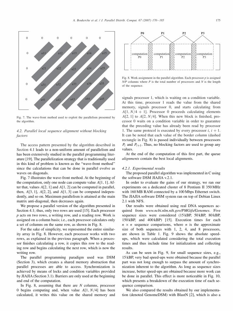
The access pattern presented by the algorithm described inSection 4.1 leads to a non-uniform amount of parallelism andhas been extensively studied in the parallel programming liter-ature [19]. The parallelization strategy that is traditionally usedin this kind of problem is known as the “wave-front method’’since the calculations that can be done in parallel evolve aswaves on diagonals.

Fig. 7 illustrates the wave-front method. At the beginning ofthe computation, only one node can compute value A[1, 1]. Af-ter that, values A[2, 1] and A[1, 2] can be computed in parallel,then, A[3, 1], A[2, 2], and A[1, 3] can be computed indepen-dently, and so on. Maximum parallelism is attained at the mainmatrix anti-diagonal, then decreases again.

We propose a parallel version of the algorithm presented inSection 4.1; thus, only two rows are used [15]. Each processorp acts on two rows, a writing row, and a reading row. Work isassigned on a column basis; i.e., each processor calculates onlya set of columns on the same row, as shown in Fig. 8.

For the sake of simplicity, we represented the entire similar-ity array in Fig. 8. However, each processor works with tworows, as explained in the previous paragraph. When a proces-sor finishes calculating a row, it copies this row to the read-ing row and begins calculating the next row, which is now thewriting row.

The parallel programming paradigm used was DSM(Section 3), which creates a shared memory abstraction thatparallel processes are able to access. Synchronization isachieved by means of locks and condition variables providedby JIAJIA (Section 3.1). Barriers are only used at the beginningand end of the computation.

In Fig. 8, assuming that there are N columns, processor0 begins computing and, when value A[1, N/4] has beencalculated, it writes this value on the shared memory and

P0 P1 P2 P3

computationP0

computationP1

computationP2

computationP3

Fig. 8. Work assignment in the parallel algorithm. Each processor p is assignedN/P columns where P is the total number of processors and N is the lengthof the sequence.

signals processor 1, which is waiting on a condition variable.At this time, processor 1 reads the value from the sharedmemory, signals processor 0, and starts calculating fromA[1, N/4 + 1]. Processor 0 proceeds calculating elementsA[2, 1] to A[2, N/4]. When this new block is finished, pro-cessor 0 waits on a condition variable in order to guaranteethat the preceding value has already been read by processor1. The same protocol is executed by every processor i, i + 1.It can be noted that each value of the border column (dashedrectangle in Fig. 8) is passed individually between processorsPi and Pi+1. Thus, no blocking factors are used to group anyvalues.

At the end of the computation of this first part, the queuealignments contain the best local alignments.

4.2.1. Experimental resultsThe proposed parallel algorithm was implemented in C using

the software DSM JIAJIA v.2.1.In order to evaluate the gains of our strategy, we ran our

experiments on a dedicated cluster of 8 Pentium II 350 MHzwith 160 MB RAM connected by a 100 Mbps Ethernet switch.The JIAJIA software DSM system ran on top of Debian Linux2.1 with NFS.

Our results were obtained using real DNA sequences ac-quired from www.ncbi.nlm.nih.gov/PMGifs/Genomes. Fivesequence sizes were considered (15 kBP, 50 kBP, 80 kBP,150 kBP, and 400 kBP) [15]. Execution times for eachn × n sequence comparisons, where n is the approximatesize of both sequences with 1, 2, 4, and 8 processors,are shown in Table 1. Fig. 9 shows the absolute speed-ups, which were calculated considering the total executiontimes and thus include time for initialization and collectingresults.

As can be seen in Fig. 9, for small sequence sizes, e.g.,15 kBP, very bad speed-ups were obtained because the parallelpart was not long enough to surpass the amount of synchro-nization inherent to the algorithm. As long as sequence sizesincrease, better speed-ups are obtained because more work canbe done in parallel. This effect is more noticeable in Fig. 10,which presents a breakdown of the execution time of each se-quence comparison.

We also compared the results obtained by our implementa-tion (denoted GenomeDSM) with BlastN [2], which is also a


Table 1Total execution times (s) for 5 sequence sizes

Size (n × n) Serial 2 proc 4 proc 8 proc

15K × 15 K 296 283.18 202.18 181.2950K × 50 K 3461 2884.15 1669.53 1107.0280K × 80 K 7967 6094.18 3370.40 2162.82150K × 150 K 24,107 19,522.95 10,377.89 5991.79400K × 400 K 175,295 141,840.98 72,770.99 38,206.84

1

2

3

4

5

6

7

8

1 2 3 4 5 6 7 8

speedup

processors

linear

15Kx15K

50Kx50K

80Kx80K

150Kx150K

400Kx400K

Fig. 9. Absolute speed-ups for DNA sequence comparison.

15K 80K50K 150K 400K

20%

40%

60%

80%

100% computation

communication

lock+cv

barrier

Fig. 10. Execution time breakdown for 5 sequence sizes, containing the rela-tive time spent in computation, communication, lock and condition variable,and barrier.

heuristic method. For this task, we used two 50 kBP mitochon-drial genomes, Allomyces acrogynus and Chaetosphaeridiumglobosum.

In Table 2, we present a comparison between these programs,showing the coordinates of the alignments with the best scores[15]. Yet, we still notice that the results obtained by both pro-grams are very close but not the same. This can be explained bythe fact that both programs use heuristics that involve differentparameters.

4.3. Parallel local sequence alignment with blocking factors

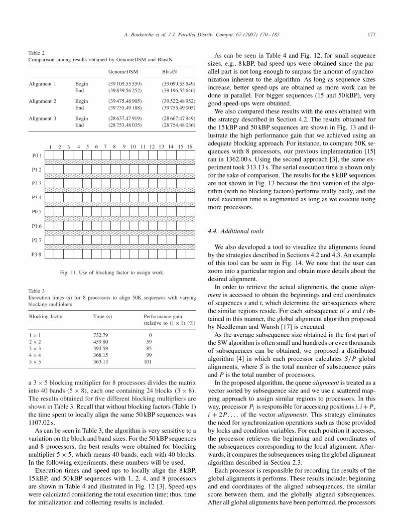
Using the wave-front method and obtaining good perfor-mance results is sometimes tricky. Therefore, it is worth inves-tigating whether the communication time can be reduced bygrouping many values from the border column (Fig. 8) into onesingle communication. This is done by means of introducingblocking factors to the strategy presented in Section 4.2.

Fig. 11 shows a sample matrix division between 4 processors.In this case, the matrix is divided into 8 bands where eachprocessor is assigned 2 bands. A band is defined as a set ofrows. Each band is subdivided into blocks; in this case thereare 16.

Since processor P0 is the only processor that is capable ofperforming calculations once the algorithm has begun, somevaluable processing power is being wasted. When P0 finishescalculating the block (1,1), it sends the last row of this blockto the next processor (P1) and begins processing block (1,2).When P1 receives the data from P0, it can start processing block(2,1). Processor P0 starts processing block (1,4) until all avail-able processing power is in use. When P0 finishes calculatingits first band, it will begin calculating block (5,1).

In our parallel strategy [3], the height of the bands and thewidth of the blocks appear to be closely related to the perfor-mance gain. Large values for height and width tend to limitthe total amount of parallelism, but very small values will beincurred in a high communication overhead since the amountof data exchanged between the processors will be greatly in-creased. The horizontal double lines in Fig. 11 show the amountof data being exchanged between the processors.

In our approach, the similar array can be divided into bandsand blocks of different heights and widths. Small chunks canbe used at the beginning of computation in order to allow theprocessors to start computing earlier. In the same way, smallchunks can also be used at the end of the computation in orderto make processors finish calculating later. When all blockshave been processed, each processor holds a queue containingthe local alignments. These alignments are then gathered andduplicate alignments removed. Each alignment indicates thestart and end point coordinates of a local alignment betweenthe sequences.

4.3.1. Experimental resultsIn order to obtain an appropriate block size, we run our

algorithm for the 50 kBP sequences, varying the block size andthe number of bands using a blocking multiplier. For instance,


Table 2Comparison among results obtained by GenomeDSM and BlastN

GenomeDSM BlastN

Alignment 1 Begin (39 109,55 559) (39 099,55 549)End (39 839,56 252) (39 196,55 646)



1 2 3 4 5 6 7 8 9 10 11 12 13 14

P3 4

P2 3

P1 2

P0 1

P0 5

P1 6

P2 7

P3 8

15 16

Fig. 11. Use of blocking factor to assign work.

Table 3Execution times (s) for 8 processors to align 50K sequences with varyingblocking multipliers

Blocking factor Time (s) Performance gain(relative to (1 × 1) (%)

1 × 1 732.79 02 × 2 459.80 593 × 3 394.59 854 × 4 368.15 995 × 5 363.13 101

a 3 × 5 blocking multiplier for 8 processors divides the matrixinto 40 bands (5 × 8), each one containing 24 blocks (3 × 8).The results obtained for five different blocking multipliers areshown in Table 3. Recall that without blocking factors (Table 1)the time spent to locally align the same 50 kBP sequences was1107.02 s.

As can be seen in Table 3, the algorithm is very sensitive to avariation on the block and band sizes. For the 50 kBP sequencesand 8 processors, the best results were obtained for blockingmultiplier 5 × 5, which means 40 bands, each with 40 blocks.In the following experiments, these numbers will be used.

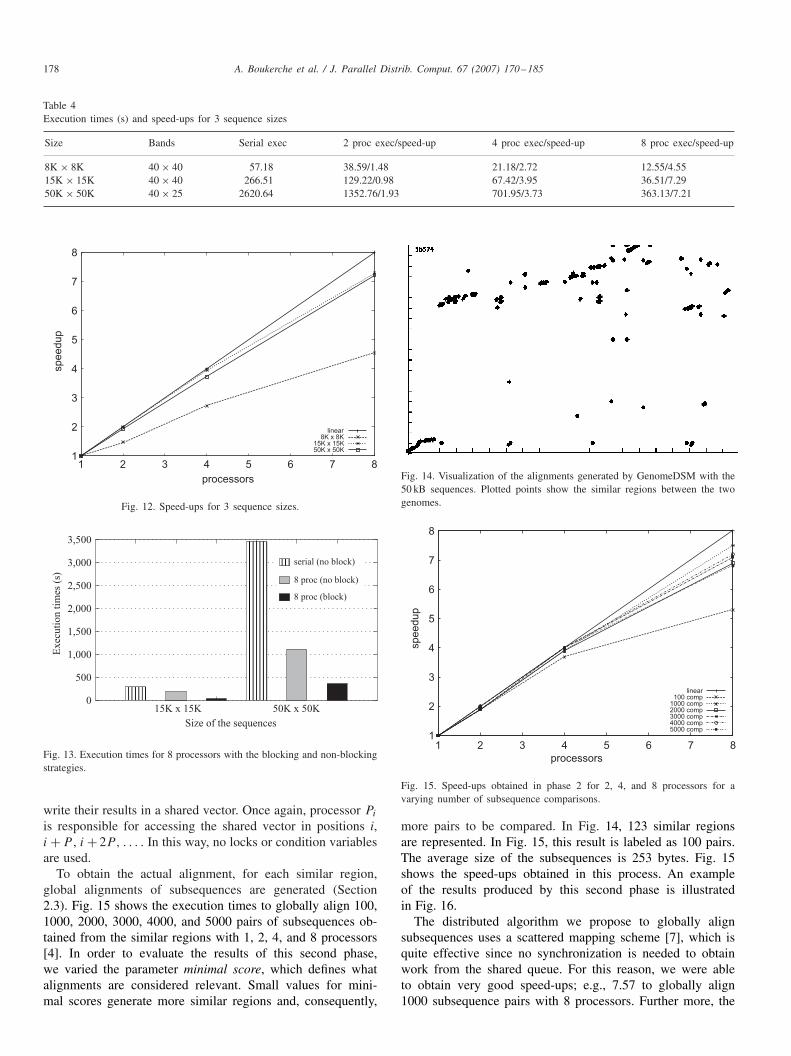
Execution times and speed-ups to locally align the 8 kBP,15 kBP, and 50 kBP sequences with 1, 2, 4, and 8 processorsare shown in Table 4 and illustrated in Fig. 12 [3]. Speed-upswere calculated considering the total execution time; thus, timefor initialization and collecting results is included.

As can be seen in Table 4 and Fig. 12, for small sequencesizes, e.g., 8 kBP, bad speed-ups were obtained since the par-allel part is not long enough to surpass the amount of synchro-nization inherent to the algorithm. As long as sequence sizesincrease, better speed-ups are obtained as more work can bedone in parallel. For bigger sequences (15 and 50 kBP), verygood speed-ups were obtained.

We also compared these results with the ones obtained withthe strategy described in Section 4.2. The results obtained forthe 15 kBP and 50 kBP sequences are shown in Fig. 13 and il-lustrate the high performance gain that we achieved using anadequate blocking approach. For instance, to compare 50K se-quences with 8 processors, our previous implementation [15]ran in 1362.00 s. Using the second approach [3], the same ex-periment took 313.13 s. The serial execution time is shown onlyfor the sake of comparison. The results for the 8 kBP sequencesare not shown in Fig. 13 because the first version of the algo-rithm (with no blocking factors) performs really badly, and thetotal execution time is augmented as long as we execute usingmore processors.

4.4. Additional tools

We also developed a tool to visualize the alignments foundby the strategies described in Sections 4.2 and 4.3. An exampleof this tool can be seen in Fig. 14. We note that the user canzoom into a particular region and obtain more details about thedesired alignment.

In order to retrieve the actual alignments, the queue align-ment is accessed to obtain the beginnings and end coordinatesof sequences s and t, which determine the subsequences wherethe similar regions reside. For each subsequence of s and t ob-tained in this manner, the global alignment algorithm proposedby Needleman and Wunsh [17] is executed.

As the average subsequence size obtained in the first part ofthe SW algorithm is often small and hundreds or even thousandsof subsequences can be obtained, we proposed a distributedalgorithm [4] in which each processor calculates S/P globalalignments, where S is the total number of subsequence pairsand P is the total number of processors.

In the proposed algorithm, the queue alignment is treated as avector sorted by subsequence size and we use a scattered map-ping approach to assign similar regions to processors. In thisway, processor Pi is responsible for accessing positions i, i+P ,i + 2P, . . . of the vector alignments. This strategy eliminatesthe need for synchronization operations such as those providedby locks and condition variables. For each position it accesses,the processor retrieves the beginning and end coordinates ofthe subsequences corresponding to the local alignment. After-wards, it compares the subsequences using the global alignmentalgorithm described in Section 2.3.

Each processor is responsible for recording the results of theglobal alignments it performs. These results include: beginningand end coordinates of the aligned subsequences, the similarscore between them, and the globally aligned subsequences.After all global alignments have been performed, the processors


Table 4Execution times (s) and speed-ups for 3 sequence sizes

Size Bands Serial exec 2 proc exec/speed-up 4 proc exec/speed-up 8 proc exec/speed-up

8K × 8K 40 × 40 57.18 38.59/1.48 21.18/2.72 12.55/4.5515K × 15K 40 × 40 266.51 129.22/0.98 67.42/3.95 36.51/7.2950K × 50K 40 × 25 2620.64 1352.76/1.93 701.95/3.73 363.13/7.21

1

2

3

4

5

6

7

8

1 2 3 4 5 6 7 8

speedup

processors

linear8K x 8K

15K x 15K50K x 50K

Fig. 12. Speed-ups for 3 sequence sizes.

0

500

1,000

1,500

2,000

2,500

3,000

3,500

Exec

uti

on t

imes

(s)

Size of the sequences

50K x 50K15K x 15K

serial (no block)

8 proc (block)

8 proc (no block)

Fig. 13. Execution times for 8 processors with the blocking and non-blockingstrategies.

write their results in a shared vector. Once again, processor Pi

is responsible for accessing the shared vector in positions i,i +P , i + 2P, . . . . In this way, no locks or condition variablesare used.

To obtain the actual alignment, for each similar region,global alignments of subsequences are generated (Section2.3). Fig. 15 shows the execution times to globally align 100,1000, 2000, 3000, 4000, and 5000 pairs of subsequences ob-tained from the similar regions with 1, 2, 4, and 8 processors[4]. In order to evaluate the results of this second phase,we varied the parameter minimal score, which defines whatalignments are considered relevant. Small values for mini-mal scores generate more similar regions and, consequently,

Fig. 14. Visualization of the alignments generated by GenomeDSM with the50 kB sequences. Plotted points show the similar regions between the twogenomes.

1

2

3

4

5

6

7

8

1 2 3 4 5 6 7 8

speedup

processors

linear100 comp

1000 comp2000 comp3000 comp4000 comp5000 comp

Fig. 15. Speed-ups obtained in phase 2 for 2, 4, and 8 processors for avarying number of subsequence comparisons.

more pairs to be compared. In Fig. 14, 123 similar regionsare represented. In Fig. 15, this result is labeled as 100 pairs.The average size of the subsequences is 253 bytes. Fig. 15shows the speed-ups obtained in this process. An exampleof the results produced by this second phase is illustratedin Fig. 16.

The distributed algorithm we propose to globally alignsubsequences uses a scattered mapping scheme [7], which isquite effective since no synchronization is needed to obtainwork from the shared queue. For this reason, we were ableto obtain very good speed-ups; e.g., 7.57 to globally align1000 subsequence pairs with 8 processors. Further more, the


initial_x: 11669 final_x: 11751

similarity: 26

align_s: CTGCAAATCCGTTAGT_TACGCCTGTA

TCTATCGTGCCTGAGTGGTACTTTTTACC_GT

TCTATGCCA_TATTAAGACTATACCA

align_t: CAGCAAATCCAAT_GTCAACACCTGCG

CATATAGTACCAGAATGGTATTTTCTACCAGT

T_TACGCAATTCTTCGCAG_TATACCA

initial_x: 8553 final_x: 8625

initial_y: 42400 final_y: 42472

similarity: 39

GGACACTAATGGGTGGCTGTAATGCTGCTTAT

GTACAGTCGGTATT

GGTTCACCGTGGGCCTGAAATGGTGCTTAAT

GTACAGTCGAAATT

align_s: G_AG_GTATACAACTTCGCTACAGAGT

align_t: GTTGTGTGTACAA_T_CGCTACAGACT

initial_y: 42964 final_y: 43046

Fig. 16. Global alignment of two subsequences generated in phase 1.

speed-up obtained apparently does not depend on the sharedqueue size. This can be seen in Fig. 15. Speed-ups for 2 and4 processors are between 2 and 1.91 and between 4 and 3.76for 100 and 5000 subsequence pairs, respectively. Speed-ups for 8 processors presented a slightly higher variation,where a speed-up of 7.57 was attained for 1000 subsequencepairs.

For 100 and 5000 subsequence pairs, speed-ups obtained for8 processors were 5.33 and 6.80, respectively. For 100 compar-isons, we also measured a speed-up of 5.33 for 7 processors.This indicates that with a reduced number of comparisons ofsmall subsequences, no benefit is obtained when increasing thenumber of processors from 7 to 8.

5. Reducing space complexity without introducingheuristics

In Sections 4.2 and 4.3, we presented two strategies that areable to locally align long DNA sequences using a heuristics-based variant of the SW algorithm. These heuristics were usedin order to reduce space complexity. The results obtained upto that point were good but we wanted to further investigatewhether it was possible to use the original SW algorithm whilestill maintaining memory requirements at a reasonable level.

The key goal of this third strategy was to calculate the similararray for local sequence alignment without introducing heuris-tics, since our objective was to execute the original SW algo-rithm without loss of information. Besides calculating the sim-ilar array, the third strategy allowed the array, either partiallyor entirely, to be saved to disk.

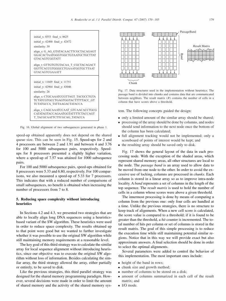
Like the previous strategies, this third parallel strategy wasdesigned for the shared memory programming paradigm. How-ever, several decisions were made in order to limit the amountof shared memory and the activity of the shared memory sys-

Chunk

Band

PassageBand

Result Matrix

Fig. 17. Data structures used in the implementation without heuristics. Thepassage band is divided into chunks and contains data that are communicatedbetween neighbors. The result matrix (R) contains the number of cells in acolumn that have scores above a threshold.

tem. The following concepts guided the design:

• only a limited amount of the similar array should be shared;• processing of the array should be done by columns, and nodes

should send information to the next node once the bottom ofthe column has been calculated;

• full alignment tracking would not be implemented; only ascoreboard of points of interest would be kept; and

• the resulting array should be saved only to disk.

Fig. 17 shows the general layout of the data in each pro-cessing node. With the exception of the shaded areas, whichrepresent shared memory areas, all other structures are local tothe node. The passage band is an array used to allow data tobe moved from one node to the other. In order to avoid the ex-cessive use of locking, columns are processed in chunks. Eachcolumn is stored in a linear array so as to improve intra-nodelocality. A band represents a set of columns in the length of thetop sequence. The result matrix is used to hold the number ofcells in a column whose scores were above a given threshold.

The innermost processing is done by means of computing acolumn from the previous one: only four cells are handled ata time. Unlike the previous strategies, there is no structure tokeep track of alignments. When a new cell score is calculated,the score value is compared to a threshold; if it is found to begreater than the threshold, a hit counter is incremented. The to-tal number of hits per column or set of columns is stored in theresult matrix. The goal of this simple processing is to reducethe execution time while still maintaining potential similar re-gions. Notice that in this way we will provide exact but alsoapproximate answers. A final selection should be done in orderto select the optimal alignments.

Several parameters were added to control the behavior ofthis implementation. The most important ones include:

• height of the band in rows;• chunk size and growth method;• number of columns to be stored on a disk;• amount of columns summarized in each cell of the result

matrix; and• I/O mode.


The size of the chunks can be set to a fixed value or growin arithmetic or geometric projections; it is possible to saveat all the columns, but in the tests only a reduced number ofcolumns were saved. In addition, it is possible to store individ-ual columns at the cost of more shared memory.

Each cell (Ri,j ) of the result matrix contains the total numberof hits from all the columns n of band i that satisfy the followingequation: �n/ip� = j , where ip is the result matrix interleaveparameter.

The columns that should be saved to disk are also controlledby the save interleave parameter ip such that any given col-umn i will be saved to disk if i �= 0 and ((i mod ip) ≡ 0).This interleave parameter can be used to increase or reduce theamount of information available in the end result. If the saveinterleave parameter is set to 1, the entire matrix will be saved,but even for small sequences this can require a huge amountof disk space. For instance, the comparison of two 10 kBP se-quences would require 400 Mbytes just for the column data.All passage bands are saved once the last of its cells has beenupdated.

There are three I/O modes. The simplest is the disabling ofany storing operation. In our case, there is no output of thealgorithm; this option was therefore used only to determinethe effect of I/O in general. The next mode is called immedi-ately, which means that once a column that should be storedto a disk is ready, it is written to a disk with a blocking I/Ooperation. The last mode, the deferred mode, means that thecolumns that should be saved are kept in the memory until allof the matrix has been calculated. Once the calculation has beendone, the data are sent to the disk. This requires more mem-ory but avoids the problem of blocking I/O in the middle ofprocessing. In all other modes, once the column is no longerneeded, it is released. This limits the total amount of memoryrequired.

Besides having ways to control the amount of data beinggrouped, the band size is controlled by three different schemes.The first determines fixed band size (or height). Another schemeuses even or equal bands so that all of the nodes have the sameamount of data to process. The final mode attempts to balancethe band size so that all bands are still close to the designatedband size according to the following equations:

bandsproc =⌈ �ssize/bsize

nnodes

⌉,

bsizedown =⌈

bsizebandsproc∗nnodes

⌉,

bsizeup =⌈

bsize(bandsproc−1)∗nnodes

⌉.

The new band size will be bsizeup or bsizedown , whichever isnearer to the original band size. The objective is to make allnodes process the same number of bands of equal size whilemaintaining the blocking concept.

5.1. Experimental results

Using the same platform described in Section 4.2.1, severaltests where made varying some of the configuration parameters.The following times were collected:

Init: Time required to start the DSM environment. This isthe time between the start of the main program and the lastsynchronization barrier before the main loop.

Core: Time required to calculate the score matrix. This is theoverall time for all the nodes.

Term: Time required for all nodes to reach the last barrierafter executing any deferred I/O.

Processing times shown in our results consider only the coretimes. This is the largest of the measured times and gives agood indication of the overall performance. The init time ismostly due to the overhead of starting the remote processes bythe DSM environment (and ran under 10 s for all tests). Thetermination time basically contains the time for deferred I/Oand the final synchronization times of the DSM environment.For the latter, the worst case was 20 s, but most likely becauseof the NFS and DSM overhead. Most termination times wereunder 7 s.

The result matrix (which holds the number of hits per blockof columns) does not provide much information about the align-ments found. It was allocated in such a way as to allow eachnode to handle writes locally.

Although little information is contained in the result matrix, itindicates interesting regions in the score matrix. If one considers1000 columns per cell in the matrix and a 1000-row band size,each cell will contain the total hits for 1,000,000 cells of thescore matrix. Therefore, having the total number of hits will hintwhether investigating further in that block of data. In certaintest runs, some of the result matrix cells indicated 300,000or more hits. This is of course dependent on gap costs andthreshold values. But values at this level indicate that 30% ofthe cells were above the threshold, so that region is very likelyto contain good alignments.

The limited visibility of the result matrix may be worthwhileif the overall performance is good. Knowing interesting areasof the matrix and having the boundary columns and rows allowone to reprocess these limited areas so as to retrieve the localalignments.

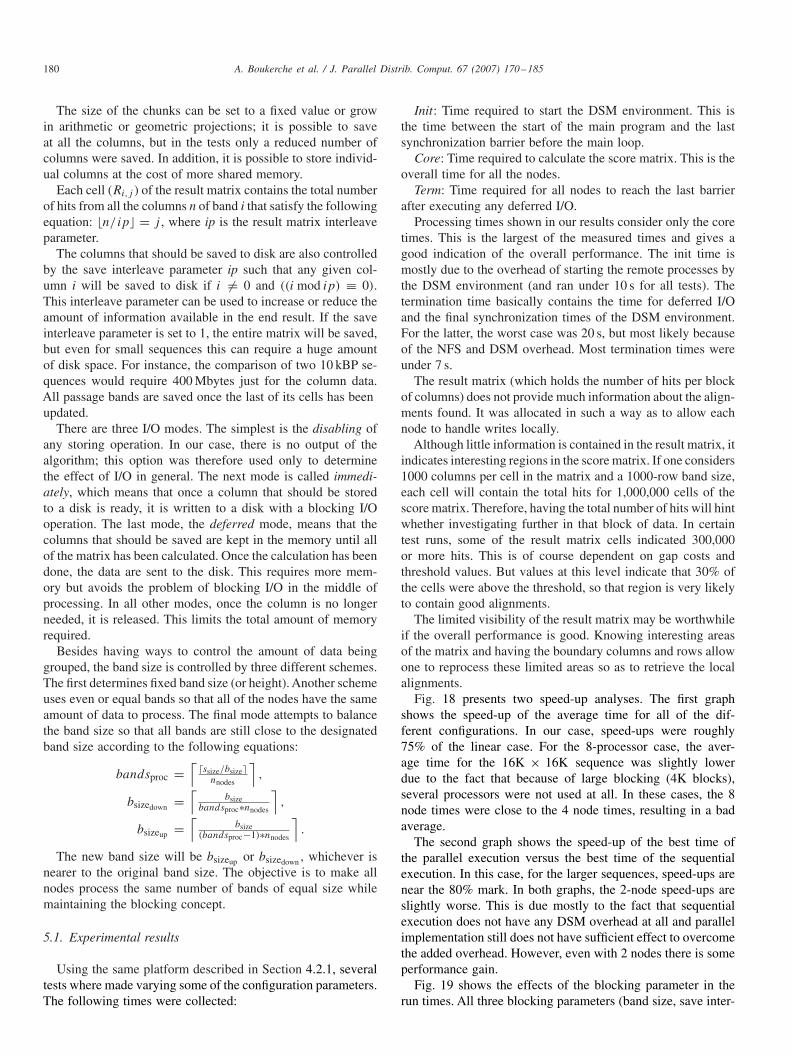
Fig. 18 presents two speed-up analyses. The first graphshows the speed-up of the average time for all of the dif-ferent configurations. In our case, speed-ups were roughly75% of the linear case. For the 8-processor case, the aver-age time for the 16K × 16K sequence was slightly lowerdue to the fact that because of large blocking (4K blocks),several processors were not used at all. In these cases, the 8node times were close to the 4 node times, resulting in a badaverage.

The second graph shows the speed-up of the best time ofthe parallel execution versus the best time of the sequentialexecution. In this case, for the larger sequences, speed-ups arenear the 80% mark. In both graphs, the 2-node speed-ups areslightly worse. This is due mostly to the fact that sequentialexecution does not have any DSM overhead at all and parallelimplementation still does not have sufficient effect to overcomethe added overhead. However, even with 2 nodes there is someperformance gain.

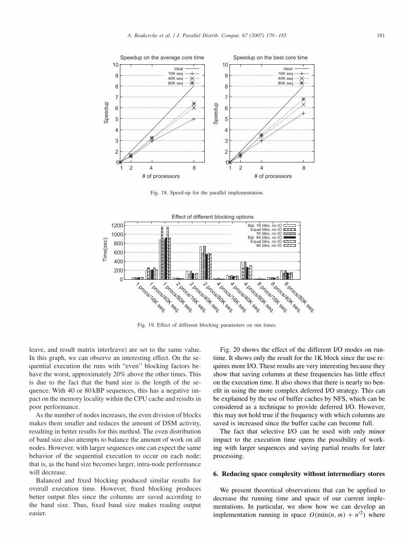
Fig. 19 shows the effects of the blocking parameter in therun times. All three blocking parameters (band size, save inter-


1

2

3

4

5

6

7

8

9

10

1 2 4 8

Speedup

# of processors

Speedup on the average core time

Ideal

16K seq

40K seq80K seq

1

2

3

4

5

6

7

8

9

10

1 2 4 8

Speedup

# of processors

Speedup on the best core time

Ideal

16K seq

40K seq80K seq

Fig. 18. Speed-up for the parallel implementation.

0

200

400

600

800

1000

1200

1 procs/16K seq.

1 procs/40K seq.

1 procs/80K seq.

2 procs/16K seq.

2 procs/40K seq.

2 procs/80K seq.

4 procs/16K seq.

4 procs/40K seq.

4 procs/80K seq.

8 procs/16K seq.

8 procs/40K seq.

8 procs/80K seq.

Tim

e(s

ec)

Effect of different blocking options

Bal. 1K blks, no IO Equal blks, no IO

1K blks, no IO Bal. 4K blks, no IO

Equal blks, no IO 4K blks, no IO

Fig. 19. Effect of different blocking parameters on run times.

leave, and result matrix interleave) are set to the same value.In this graph, we can observe an interesting effect. On the se-quential execution the runs with “even’’ blocking factors be-have the worst, approximately 20% above the other times. Thisis due to the fact that the band size is the length of the se-quence. With 40 or 80 kBP sequences, this has a negative im-pact on the memory locality within the CPU cache and results inpoor performance.

As the number of nodes increases, the even division of blocksmakes them smaller and reduces the amount of DSM activity,resulting in better results for this method. The even distributionof band size also attempts to balance the amount of work on allnodes. However, with larger sequences one can expect the samebehavior of the sequential execution to occur on each node;that is, as the band size becomes larger, intra-node performancewill decrease.

Balanced and fixed blocking produced similar results foroverall execution time. However, fixed blocking producesbetter output files since the columns are saved according tothe band size. Thus, fixed band size makes reading outputeasier.

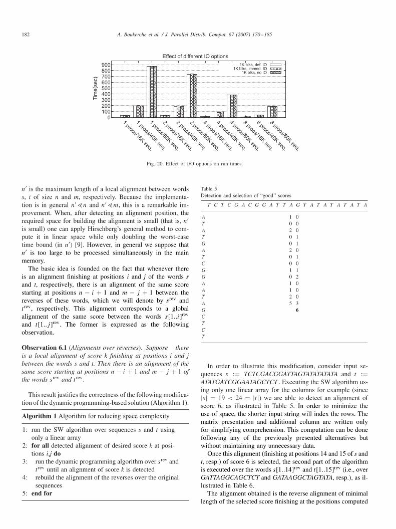
Fig. 20 shows the effect of the different I/O modes on run-time. It shows only the result for the 1K block since the use re-quires more I/O. These results are very interesting because theyshow that saving columns at these frequencies has little effecton the execution time. It also shows that there is nearly no ben-efit in using the more complex deferred I/O strategy. This canbe explained by the use of buffer caches by NFS, which can beconsidered as a technique to provide deferred I/O. However,this may not hold true if the frequency with which columns aresaved is increased since the buffer cache can become full.

The fact that selective I/O can be used with only minorimpact to the execution time opens the possibility of work-ing with larger sequences and saving partial results for laterprocessing.

6. Reducing space complexity without intermediary stores

We present theoretical observations that can be applied todecrease the running time and space of our current imple-mentations. In particular, we show how we can develop animplementation running in space O(min(n, m) + n′2) where


0 100 200 300 400 500 600 700 800 900

1 procs/16K seq.

1 procs/40K seq.

1 procs/80K seq.

2 procs/16K seq.

2 procs/40K seq.

2 procs/80K seq.

4 procs/16K seq.

4 procs/40K seq.

4 procs/80K seq.

8 procs/16K seq.

8 procs/40K seq.

8 procs/80K seq.

Tim

e(s

ec)

Effect of different IO options

1K blks, def. IO 1K blks, immed. IO

1K blks, no IO

Fig. 20. Effect of I/O options on run times.

n′ is the maximum length of a local alignment between wordss, t of size n and m, respectively. Because the implementa-tion is in general n′>n and n′>m, this is a remarkable im-provement. When, after detecting an alignment position, therequired space for building the alignment is small (that is, n′is small) one can apply Hirschberg’s general method to com-pute it in linear space while only doubling the worst-casetime bound (in n′) [9]. However, in general we suppose thatn′ is too large to be processed simultaneously in the mainmemory.

The basic idea is founded on the fact that whenever thereis an alignment finishing at positions i and j of the words sand t, respectively, there is an alignment of the same scorestarting at positions n − i + 1 and m − j + 1 between thereverses of these words, which we will denote by srev andt rev, respectively. This alignment corresponds to a globalalignment of the same score between the words s[1..i]rev

and t[1..j ]rev. The former is expressed as the followingobservation.

Observation 6.1 (Alignments over reverses). Suppose thereis a local alignment of score k finishing at positions i and jbetween the words s and t. Then there is an alignment of thesame score starting at positions n − i + 1 and m − j + 1 ofthe words srev and t rev.

This result justifies the correctness of the following modifica-tion of the dynamic programming-based solution (Algorithm 1).

Algorithm 1 Algorithm for reducing space complexity

1: run the SW algorithm over sequences s and t usingonly a linear array

2: for all detected alignment of desired score k at posi-tions i,j do

3: run the dynamic programming algorithm over srev andt rev until an alignment of score k is detected

4: rebuild the alignment of the reverses over the originalsequences

5: end for

Table 5Detection and selection of “good’’ scores

T C T C G A C G G A T T A G T A T A T A T A T A

A 1 0T 0 0A 2 0T 0 1G 0 1A 2 0T 0 1C 0 0G 1 1G 0 2A 1 0A 1 0T 2 0A 5 3G 6C

T

C

T

In order to illustrate this modification, consider input se-quences s := TCTCGACGGATTAGTATATATATA and t :=ATATGATCGGAATAGCTCT . Executing the SW algorithm us-ing only one linear array for the columns for example (since|s| = 19 < 24 = |t |) we are able to detect an alignment ofscore 6, as illustrated in Table 5. In order to minimize theuse of space, the shorter input string will index the rows. Thematrix presentation and additional column are written onlyfor simplifying comprehension. This computation can be donefollowing any of the previously presented alternatives butwithout maintaining any unnecessary data.

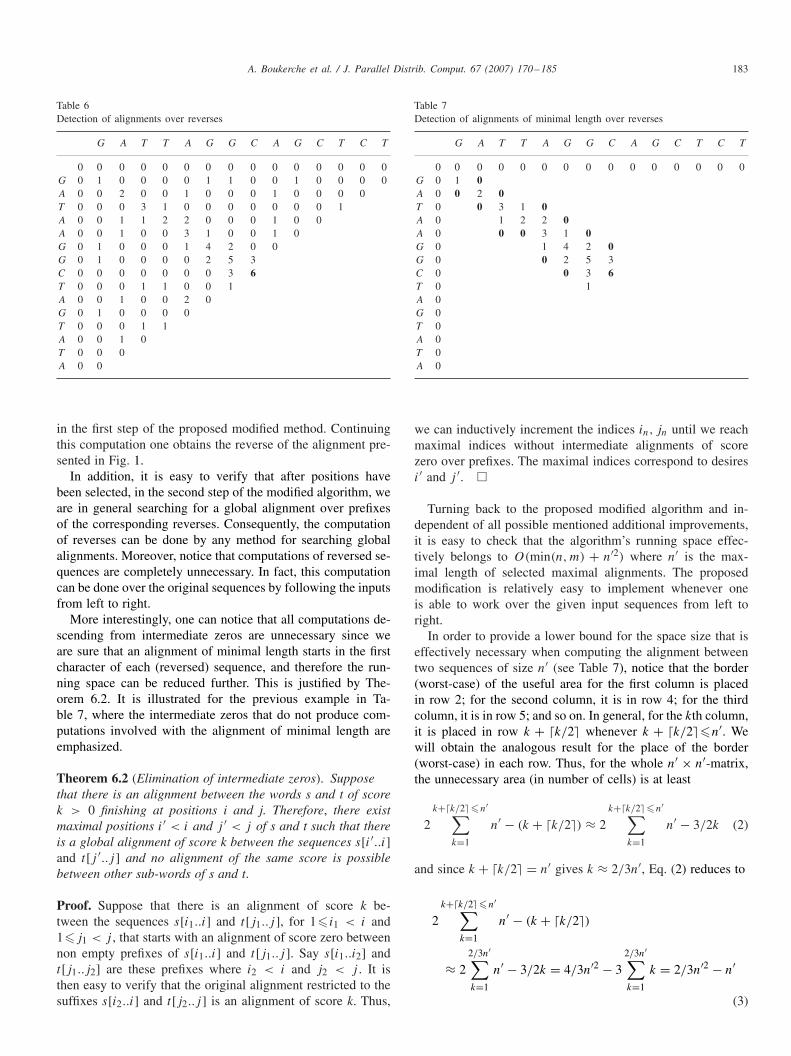
Once this alignment (finishing at positions 14 and 15 of s andt, resp.) of score 6 is selected, the second part of the algorithmis executed over the words s[1..14]rev and t[1..15]rev (i.e., overGATTAGGCAGCTCT and GATAAGGCTAGTATA, resp.), as il-lustrated in Table 6.

The alignment obtained is the reverse alignment of minimallength of the selected score finishing at the positions computed


Table 6Detection of alignments over reverses

G A T T A G G C A G C T C T

0 0 0 0 0 0 0 0 0 0 0 0 0 0 0G 0 1 0 0 0 0 1 1 0 0 1 0 0 0 0A 0 0 2 0 0 1 0 0 0 1 0 0 0 0T 0 0 0 3 1 0 0 0 0 0 0 0 1A 0 0 1 1 2 2 0 0 0 1 0 0A 0 0 1 0 0 3 1 0 0 1 0G 0 1 0 0 0 1 4 2 0 0G 0 1 0 0 0 0 2 5 3C 0 0 0 0 0 0 0 3 6T 0 0 0 1 1 0 0 1A 0 0 1 0 0 2 0G 0 1 0 0 0 0T 0 0 0 1 1A 0 0 1 0T 0 0 0A 0 0

in the first step of the proposed modified method. Continuingthis computation one obtains the reverse of the alignment pre-sented in Fig. 1.

In addition, it is easy to verify that after positions havebeen selected, in the second step of the modified algorithm, weare in general searching for a global alignment over prefixesof the corresponding reverses. Consequently, the computationof reverses can be done by any method for searching globalalignments. Moreover, notice that computations of reversed se-quences are completely unnecessary. In fact, this computationcan be done over the original sequences by following the inputsfrom left to right.

More interestingly, one can notice that all computations de-scending from intermediate zeros are unnecessary since weare sure that an alignment of minimal length starts in the firstcharacter of each (reversed) sequence, and therefore the run-ning space can be reduced further. This is justified by The-orem 6.2. It is illustrated for the previous example in Ta-ble 7, where the intermediate zeros that do not produce com-putations involved with the alignment of minimal length areemphasized.

Theorem 6.2 (Elimination of intermediate zeros). Supposethat there is an alignment between the words s and t of scorek > 0 finishing at positions i and j. Therefore, there existmaximal positions i′ < i and j ′ < j of s and t such that thereis a global alignment of score k between the sequences s[i′..i]and t[j ′..j ] and no alignment of the same score is possiblebetween other sub-words of s and t.

Proof. Suppose that there is an alignment of score k be-tween the sequences s[i1..i] and t[j1..j ], for 1� i1 < i and1�j1 < j , that starts with an alignment of score zero betweennon empty prefixes of s[i1..i] and t[j1..j ]. Say s[i1..i2] andt[j1..j2] are these prefixes where i2 < i and j2 < j . It isthen easy to verify that the original alignment restricted to thesuffixes s[i2..i] and t[j2..j ] is an alignment of score k. Thus,

Table 7Detection of alignments of minimal length over reverses

G A T T A G G C A G C T C T

0 0 0 0 0 0 0 0 0 0 0 0 0 0 0G 0 1 0A 0 0 2 0T 0 0 3 1 0A 0 1 2 2 0A 0 0 0 3 1 0G 0 1 4 2 0G 0 0 2 5 3C 0 0 3 6T 0 1A 0G 0T 0A 0T 0A 0

we can inductively increment the indices in, jn until we reachmaximal indices without intermediate alignments of scorezero over prefixes. The maximal indices correspond to desiresi′ and j ′. �

Turning back to the proposed modified algorithm and in-dependent of all possible mentioned additional improvements,it is easy to check that the algorithm’s running space effec-tively belongs to O(min(n, m) + n′2) where n′ is the max-imal length of selected maximal alignments. The proposedmodification is relatively easy to implement whenever oneis able to work over the given input sequences from left toright.

In order to provide a lower bound for the space size that iseffectively necessary when computing the alignment betweentwo sequences of size n′ (see Table 7), notice that the border(worst-case) of the useful area for the first column is placedin row 2; for the second column, it is in row 4; for the thirdcolumn, it is in row 5; and so on. In general, for the kth column,it is placed in row k + �k/2 whenever k + �k/2�n′. Wewill obtain the analogous result for the place of the border(worst-case) in each row. Thus, for the whole n′ × n′-matrix,the unnecessary area (in number of cells) is at least

2k+�k/2�n′∑

k=1

n′ − (k + �k/2) ≈ 2k+�k/2�n′∑

k=1

n′ − 3/2k (2)

and since k + �k/2 = n′ gives k ≈ 2/3n′, Eq. (2) reduces to

2k+�k/2�n′∑

k=1

n′ − (k + �k/2)

≈ 22/3n′∑k=1

n′ − 3/2k = 4/3n′2 − 32/3n′∑k=1

k = 2/3n′2 − n′

(3)


from which we can conclude that the necessary space (worst-case) of the whole n′ × n′-matrix is approximately 30%.

7. Conclusion and future work

In this paper, we proposed and evaluated three parallel strate-gies to solve the DNA local sequence alignment problem. ADSM system was chosen since, for this kind of problem, DSMoffers an easier programming model than its message-passingcounterpart.

The first two strategies (heuristic and heuristic_block) usedheuristics to reduce the space complexity to O(n) where n isthe size of the sequences to be compared. The third strategy(pre_process) allowed the original SW algorithm to be run bysaving information about the most relevant columns of the re-sult matrix to disk. These columns were later processed in orderto retrieve the actual alignments. For all strategies, the wave-front method was used and work was assigned on a column orrow basis. Synchronization was achieved with locks and con-dition variables. Barriers were only used at the beginning andat the end of computation.

The results obtained to locally align real DNA sequences inan eight-machine cluster present good speed-ups that are im-proved depending on the strategy used. For instance, in or-der to compare two sequences of approximately 400 kBP us-ing the heuristic approach, we obtained a 4.58 speed-up ofthe total execution time, reducing execution time from 2 daysto 10 h.

Our results also show that an appropriate blocking fac-tor can further reduce the execution time for obtaining lo-cal alignments. Moreover, using a third strategy that doesnot keep track of the candidate alignments can also providea great performance gain at the expense of storing certainintermediate columns to disk. We also presented some the-oretical results that eliminate the need for disk storage bymaintaining only the coordinates of the highest score and re-trieving the actual alignments over the reverses of the originalsequences.

In terms of immediate future work, we intend to implementthe modifications suggested in Section 6. Furthermore, we in-tend to run this modified algorithm in order to compare verylong DNA sequences (larger than 1 MBP) in a heterogenouscluster. In this case, message-passing will be used for inter-cluster communication and DSM will be used for communicat-ing processes that belong to the same cluster.

References

[1] S. Adve, Designing memory consistency models for shared-memorymultiprocessors, Ph.D. Thesis, University of Wisconsin-Madison, 1993,233p.

[2] S.F. Altschul, et al., Gapped blast and psi-blast: a new generation ofprotein database search programs, Nucleic Acids Res. 25 (17) (1997)3389–3402.

[3] R. Batista, D. Silva, A.C. Melo, L. Weigang, Using a DSM applicationto locally align DNA sequences, in: International Workshop on SoftwareDSM on Clusters (WSDSM) held in conjunction with InernationalConference of Cluster Computing and the Grid (CCGrid), IEEEComputer Society, 2004, pp. 372–378.

[4] A. Bouckerche, A.C. Melo, M.E. Walter, R. Melo, M. Nardelli, P.Santana, R. Batista, T. Martins, Local DNA sequence alignment in acluster of workstations, in: International Workshop on Nature InspiredDistributed Computing (NIDISC’04) held in conjunction with theInternational Parallel and Distributed Processing Symposium (IPDPS),IEEE Computer Society, 2004.

[5] Decypher Co., Decypher Smith–Waterman Solution, 2003.[6] DISC group, Smith and Waterman Homology Search, 2003.[7] I. Foster, Designing and Building Parallel Programs, Addison-Wesley,

Reading, MA, 1995.[8] K. Gharachorloo, Memory consistency and event ordering in scalable

shared-memory multiprocessors, in: International Symposium onComputer Architecture (ISCA), ACM, 1990, pp. 15–24.

[9] D.S. Hirschberg, Algorithms for the Longest Common SubsequenceProblem, J. ACM 24 (4) (1977) 664–675.

[10] S. Hu, W. Shi, Z. Tang, Jiajia: an SVM system based on a new cachecoherence protocol, in: High Performance Computing and Networking(HPCN), Springer, Berlin, 1999, pp. 463–472.

[11] W. Hu, W. Shi, Jiajia user’s manual, Technical Report, Chinese Academyof Sciences, 1999.

[12] L. Iftode, J. Singh, K. Li, Scope consistency: bridging the gap betweenrelease consistency and entry consistency, in: Eighth ACM SPAA’96,ACM, 1996, pp. 277–287.

[13] K. Li, Shared virtual memory on loosely coupled architectures, Ph.D.Thesis, Yale University, 1986.

[14] W.S. Martins, J.B. Del Cuvillo, F.J. Useche, K.B. Theobald, G.R.Gao, A multithread parallel implementation of a dynamic programmingalgorithm for sequence comparison, in: Brazilian Symposium onComputer Architecture and High Performance Computing (SBAC-PAD),2001, pp. 1–8.

[15] R.C. Melo, M.E. Walter, A.C. Melo, R. Batista, M. Nardelli, T. Martins,T. Fonseca, Comparing two long biological sequences using a DSMsystem, Euro-Par 2003: Parallel Processing, Lecture Notes in ComputerScience, vol. 2790, Springer, Berlin, 2003, pp. 517–524.

[16] D. Mosberger, Memory consistency models, Operating Systems Review,1993, 18–26.

[17] S.B. Needleman, C.D. Wunsh, A general method applicable to the searchof similarities of amino acid sequences of two proteins, J. MolecularBiol. (48) (1970) 443–453.

[18] W.R. Pearson, D.L. Lipman, Improved tools for biological sequencecomparison, Proc. Nat. Acad. Sci. U.S.A. (1988) 2444–2448.

[19] G. Pfister, In Search of Clusters—The Coming Battle for Lowly ParallelComputing, Prentice-Hall, Englewood Cliffs, NJ, 1995.

[20] J.C. Setubal, J. Meidanis, Introduction to Computational MolecularBiology, Brooks/Cole Publishing Company, 1997.

[21] T.F. Smith, M.S. Waterman, Identification of common molecular sub-sequences, J. Molecular Biol. (147) (1981) 195–197.

Azzedine Boukerche is a Full Professor andholds a Canada Research Chair position indistributed simulation and wireless and mobilenetworking at the University of Ottawa. He isthe Founding Director of PARADISE ResearchLaboratory at Ottawa U. Prior to this, he helda faculty position at the University of NorthTexas, USA. He worked as a Senior Scientistat the Simulation Sciences Division, MetronCorporation located in San Diego. He was alsoemployed as a Faculty at the School of Com-puter Science McGill University, and taught at

Polytechnic of Montreal. He spent a year at the JPL/NASA-California In-stitute of Technology where he contributed to a project centered about thespecification and verification of the software used to control interplanetaryspacecraft operated by JPL/NASA Laboratory.

His current research interests include sensor networks, mobile ad hoc net-works, mobile and pervasive computing, wireless multimedia, QoS serviceprovisioning, performance evaluation and modeling of large-scale distributedsystems, distributed computing, large-scale distributed interactive simulation,and parallel discrete event simulation. Dr. Boukerche has published severalresearch papers in these areas.


Dr. Boukerche is the recipient of the Ontario Early Researcher Award (pre-viously known as Premier of Ontario Research Excellence Award (PREA)),the Canada Research Chair, the G. S. Glinski Award for Excellence inResearch, and the Ontario Distinguished Researcher Award. He was the re-cipient of the Best Research Paper Award at IEEE/ACM PADS’97, and therecipient of the 3rd National Award for Telecommunication Software 1999 forhis work on a distributed security systems on mobile phone operations, andhas been nominated for the best paper award at the IEEE/ACM PADS’99,ACM MSWiM 2001, and ACM MobiWac 2004.

He is a Co-Founder of QShine International Conference, on Quality ofService for Wireless/Wired Heterogeneous Networks (QShine 2004), servedas a General Chair for several conferences, such as ACM/IEEE MASCOST1998, IEEE DS-RT 1999–2000, ACM MSWiM 2000; Program Chair forACM/IFIPS Europar 2002, IEEE/SCS Annual Simulation Symposium ANNS2002, ACM WWW’02, IEEE/ACM MASCOTS 2002, IEEE Wireless LocalNetworks WLN 03–04; IEEE Wireless, Mobile ad hoc and Sensor Networks(IPDPS/WMAN) 04–05, ACM Modeling, Analysis and Simulation of Wire-less and Mobile Systems (MSWiM) 98–99, and TPC member of numerousIEEE and ACM conferences related to wireless communication, mobile com-puting, ad hoc and sensor networks, and distributed systems. He served as aGuest Editor for the Journal of Parallel and Distributed Computing (JPDC)(Special Issue for Routing for Mobile Ad hoc, Special Issue for wireless com-munication and mobile computing, Special Issue for mobile ad hoc network-ing and computing), and ACM/kluwer Wireless Networks and ACM/KluwerMobile Networks Applications, and the Journal of Wireless Communicationand Mobile Computing.

Dr. A. Boukerche serves as an Associate Editor and is on the EditorialBoard for ACM/Springer Wireless Networks, Wiley International Journal ofWireless Communication and Mobile Computing, the Journal of Parallel andDistributed Computing, and the SCS Transactions on simulation. He alsoserves as a Steering Committee Chair for the ACM Modeling, Analysis andSimulation for Wireless and Mobile Systems Symposium, the ACM Workshopon Performance Evaluation of Wireless Ad Hoc, Sensor, and Ubiquitous Net-works, the IEEE Workshop on Performance and Management of Wirelessand Mobile Networks, and the IEEE Distributed Simulation and Real-TimeApplications Symposium (DS-RT).

Alba Cristina M.A. Melo received her Ph.D.in Computer Science from the Institut NationalPolytechnique de Grenoble (INPG), France, in1996, her M.S. in Computer Science from Fed-eral University of Rio Grande do Sul, Brazil, in1991, and her B.S. in Computer Science fromthe University of Brasilia, Brazil, in 1986. Sheis currently an associate professor in the Com-puter Science Department at the University ofBrasilia, Brazil. Her research interests includedistributed shared memory, load balancing, clus-ter computing, grid computing, and computa-tional biology. She is a senior member of theIEEE Society.

Mauricio Ayala-Rincón received his B.S. de-grees in Computer Engineering and Mathemat-ics in the Universidad de Los Andes, Colombiain 1985 and 1987, respectively, and his Dr. rer.nat. degree in Computer Science from the Uni-versität Kaiserslautern in 1993. He is a professorin the Mathematics and Computer Science De-partments at the University of Brasilia (UnB),the vice-head of the former Department and theleader of the Group of Theory of Computationof his university. His current research focuseson algorithms, term rewriting systems, logic andsemantics of programming languages and their

applications in formal specification, and verification of computer systems. Heis a member of the European Association for Theory of Computation EATCS.

Maria Emilia Machado Telles Walter re-ceived her Ph.D. in Computer Science from theUniversity of Campinas, Brazil, in 1999, herM.S. and B.S. in Mathematics, at the Departe-ment of Mathematics from the University ofBrasilia in 1980 and 1986, respectively. Sheis a professor and the vice-had of the Com-puter Science Department at the University ofBrasilia, Brazil. She has been working since2000 in genome sequencing projects. Her re-search interests include distributed computationfor bioinformatics applications, comparitve ge-nomics and genome rearrangements. She is amember of the special committee on Com-putational Biology of the Brazilian ComputerSociety.

Parallel Strategies for Local Biological Sequence Alignment in a Cluster of Workstations

Documents

Parallel Strategies for Local Biological Sequence Alignment in a Cluster of Workstations