TALLINN UNIVERSITY OF TECHNOLOGYSchool of Information Technologies
Tarmo Prillop 178206IASM
OBSERVER BASED SENSORLESSCONTROL OF SMALL BLDC MOTORS
Master’s Thesis
Supervisor: Eduard Petlenkov
PhD
Tallinn 2019
TALLINNA TEHNIKAÜLIKOOLInfotehnoloogia teaduskond
Tarmo Prillop 178206IASM
OLEKUTAASTAJAL PÕHINEVANDURITETA JUHTIMINE VÄIKESTELE
BLDC MOOTORITELE
Magistritöö
Juhendaja: Eduard Petlenkov
PhD
Tallinn 2019

Author’s declaration of originality
I hereby certify that I am the sole author of this thesis. All the used materials, referencesto the literature and the work of others have been referred to. This thesis has not beenpresented for examination anywhere else.
Author: Tarmo Prillop
06.05.2019
3

Abstract
The aim of this thesis is to create an implementation of an observer based sensorless speedcontroller for brushless DC motors. Initially theoretical aspects of three phase motors,inverters and observer based control are described. Additionally an overview of state ofthe art in sensorless observer based control is given.
Further sections give overview of the physical hardware designed and used during thecourse of the work. The main practical part of the work was divided into two. At firstmeasurement procedures and results are presented for motor parameters as they are es-sential in model based control approaches, which observer based control is. Secondly asuitable observer based algorithm is chosen from the available research and implementedas a program on the microcontroller.
The performance analysis of the final controller showed that the chosen algorithm per-forms well even though not specifically designed for brushless DC motors.
This thesis is written in English and is 62 pages long, including 5 chapters, 39 figures,and 5 tables.
4

Annotatsioon
Käesoleva töö eesmärgiks oli luua olekutaastajal põhinev kontroller väikestele harjav-abadele alalisvoolumootoritele. Töö alguses tuuakse välja olulisemad teoreetilised as-pektid kolmefaasiliste mootorite, nende juhtelektroonika ning levinematute juhtimisalgo-ritmide kohta. Seejärel kirjeldatakse süsteemide juhtimist olekutaastajaga ning tehakseülevaade viimastest teaduspublikatsioonidest selle valdkonna kohta.
Töö praktilise osa kirjeldamine algab disainitud riistvara ning kasutatud mootorite kirjel-damisest. Seejärel selgitatakse mootorite elektriliste parameetrite mõõtmiste põhimõtteidning tuuakse välja mõõtmistulemused kasutatavate mootorite parameetrite kohta. See-järel põhjendatakse olekutaastaja valikut ning kirjeldatakse valitud olekutaastaja struktu-uri ning valemeid millel see põhineb.
Töö lõpus esitatakse mõõtmistulemused loodud kontrolleri käitumisest ning analüüsi-takse neid ning nende vastavust püstitatud nõuetele. Analüüsi tulemustest lähtuvalt olitöö edukas ning mootori juhtimine vastas juhtimiskriteeriumidele ning oli stabiilne.
Lõputöö on kirjutatud inglise keeles ning sisaldab teksti 62 leheküljel, 5 peatükki,39 joonist, 5 tabelit.
5

List of abbreviations and terms
AC Alternating current
ADALINE Adaptive linear neural network
BLDC Brushless DC motor
CSV Comma separated value
DAC Digital to analog converter
DC Direct current
DTC Direct torque control
EMF Electromotive force
FOC Field oriented control
MOSFET Metal oxide semiconductor field-effect transistor
PLL Phase lock loop
PMSM Permanent magnet synchronous motor
PWM Pulse width modulation
RPM Revolutions per minute
SPMSM Surface permanent magnet synchronous motor
SVM Space vector modulation
6
Contents
1 Introduction 13
1.1 Problem and end goal definition . . . . . . . . . . . . . . . . . . . . . . 13
1.2 Methodology . . . . . . . . . . . . . . . . . . . . . . . . . . . . . . . . 14
2 Theoretical overview 15
2.1 Three phase synchronous motors . . . . . . . . . . . . . . . . . . . . . . 15
2.2 Main control principles . . . . . . . . . . . . . . . . . . . . . . . . . . . 17
2.3 Three phase inverters . . . . . . . . . . . . . . . . . . . . . . . . . . . . 21
2.4 Space-vector modulation . . . . . . . . . . . . . . . . . . . . . . . . . . 23
2.5 Observer based control . . . . . . . . . . . . . . . . . . . . . . . . . . . 24
2.5.1 State of the art . . . . . . . . . . . . . . . . . . . . . . . . . . . 25
3 Hardware overview 27
3.1 Motor controller . . . . . . . . . . . . . . . . . . . . . . . . . . . . . . . 27
3.1.1 Microcontroller . . . . . . . . . . . . . . . . . . . . . . . . . . . 28
3.1.2 Three phase inverter and gate driver . . . . . . . . . . . . . . . . 29
3.1.3 Phase current sensing . . . . . . . . . . . . . . . . . . . . . . . . 29
3.2 Used motors and test fixture . . . . . . . . . . . . . . . . . . . . . . . . 31
4 Motor parameter measurement 34
4.1 Stator phase resistance . . . . . . . . . . . . . . . . . . . . . . . . . . . 34
4.2 Stator phase inductance . . . . . . . . . . . . . . . . . . . . . . . . . . . 36
4.3 Flux linkage . . . . . . . . . . . . . . . . . . . . . . . . . . . . . . . . . 39
7
5 Observer based controller for BLDC motor 42
5.1 Controller requirements . . . . . . . . . . . . . . . . . . . . . . . . . . . 42
5.2 Observer selection . . . . . . . . . . . . . . . . . . . . . . . . . . . . . 42
5.2.1 Ortega’s observer based angle estimation . . . . . . . . . . . . . 43
5.3 Phase-lock loop based velocity calculation . . . . . . . . . . . . . . . . . 45
5.4 Implementation . . . . . . . . . . . . . . . . . . . . . . . . . . . . . . . 46
5.4.1 Observer implementation . . . . . . . . . . . . . . . . . . . . . . 47
5.4.2 PLL implementation . . . . . . . . . . . . . . . . . . . . . . . . 48
5.4.3 PID controller implementation . . . . . . . . . . . . . . . . . . . 49
5.4.4 Motor startup procedure . . . . . . . . . . . . . . . . . . . . . . 50
5.4.5 Rotational direction reversal . . . . . . . . . . . . . . . . . . . . 53
6 Performance evaluation 54
6.1 Quadrature axis current regulator . . . . . . . . . . . . . . . . . . . . . . 54
6.2 Angle estimation accuracy . . . . . . . . . . . . . . . . . . . . . . . . . 56
6.3 Angular velocity phase lock loop . . . . . . . . . . . . . . . . . . . . . . 57
6.4 Speed controller step response . . . . . . . . . . . . . . . . . . . . . . . 58
6.5 Speed controller disturbance rejection . . . . . . . . . . . . . . . . . . . 59
7 Summary 60
References 61
Appendix 1 – Schematic prints of developed controller 63
Appendix 2 – Resistance measurement algorithm 74
8

Appendix 3 – Inductance measurement algorithm 76
Appendix 4 – Source code 78
9
List of Figures
1 BLDC motor with outside rotor [3] . . . . . . . . . . . . . . . . . . . . . 16
2 Three phase motor control schemes [6] . . . . . . . . . . . . . . . . . . . 18
3 Field oriented control scheme . . . . . . . . . . . . . . . . . . . . . . . . 20
4 Three phase two level inverter with MOSFETs . . . . . . . . . . . . . . . 21
5 Vector diagram . . . . . . . . . . . . . . . . . . . . . . . . . . . . . . . 23
6 Principle of observer based control . . . . . . . . . . . . . . . . . . . . . 25
7 Developed motor controller PCB . . . . . . . . . . . . . . . . . . . . . . 27
8 STM32F446 microcontroller block diagram [13] . . . . . . . . . . . . . 28
9 Current sense amplifier within DRV8305 IC [14] . . . . . . . . . . . . . 30
10 Current measurement calibration data . . . . . . . . . . . . . . . . . . . 31
11 Nanotec DF45 motor [15] . . . . . . . . . . . . . . . . . . . . . . . . . . 32
12 NTM 3536 910kv motor [17] . . . . . . . . . . . . . . . . . . . . . . . . 32
13 Mechanical setup used to conduct experiments . . . . . . . . . . . . . . . 33
14 Resistance measurement configuration . . . . . . . . . . . . . . . . . . . 34
15 Nanotec motor phase resistance . . . . . . . . . . . . . . . . . . . . . . . 35
16 NTM motor phase resistance . . . . . . . . . . . . . . . . . . . . . . . . 36
17 Impedance triangle for inductive loads . . . . . . . . . . . . . . . . . . . 36
18 Measurement . . . . . . . . . . . . . . . . . . . . . . . . . . . . . . . . 37
19 Nanotec motor phase inductance . . . . . . . . . . . . . . . . . . . . . . 38
20 NTM motor phase inductance . . . . . . . . . . . . . . . . . . . . . . . 39
21 Measurement setup . . . . . . . . . . . . . . . . . . . . . . . . . . . . . 40
22 Nanotec motor flux linkage . . . . . . . . . . . . . . . . . . . . . . . . . 40
23 NTM motor flux linkage . . . . . . . . . . . . . . . . . . . . . . . . . . 41
10
24 Velocity calculation PLL [19] . . . . . . . . . . . . . . . . . . . . . . . . 45
25 Observer based controller block diagram . . . . . . . . . . . . . . . . . . 46
26 Observer implementation . . . . . . . . . . . . . . . . . . . . . . . . . . 47
27 PLL implementation . . . . . . . . . . . . . . . . . . . . . . . . . . . . 48
28 PID controller implementation . . . . . . . . . . . . . . . . . . . . . . . 49
29 Scalar control . . . . . . . . . . . . . . . . . . . . . . . . . . . . . . . . 50
30 Startup graph . . . . . . . . . . . . . . . . . . . . . . . . . . . . . . . . 51
31 Scalar control to sensorless transition . . . . . . . . . . . . . . . . . . . . 51
32 Sensorless to scalar transition . . . . . . . . . . . . . . . . . . . . . . . . 52
33 Speed reversal and transitioning between critical regions . . . . . . . . . 53
34 Quadrature axis controller step response . . . . . . . . . . . . . . . . . . 54
35 Quadrature axis controller step response . . . . . . . . . . . . . . . . . . 55
36 Observer angle estimation error . . . . . . . . . . . . . . . . . . . . . . . 56
37 Speed (PLL) estimation accuracy . . . . . . . . . . . . . . . . . . . . . . 57
38 Speed controller step response . . . . . . . . . . . . . . . . . . . . . . . 58
39 Speed controller disturbance rejection . . . . . . . . . . . . . . . . . . . 59
11
List of Tables
1 Three phase inverter state table . . . . . . . . . . . . . . . . . . . . . . . 22
2 Nanotec DF45 motor parameters [16] . . . . . . . . . . . . . . . . . . . 32
3 NTM 3536 910kv motor parameters [17] . . . . . . . . . . . . . . . . . . 32
4 PLL PI regulator parameters . . . . . . . . . . . . . . . . . . . . . . . . 48
5 PID regulator parameters used . . . . . . . . . . . . . . . . . . . . . . . 49
12
1 Introduction
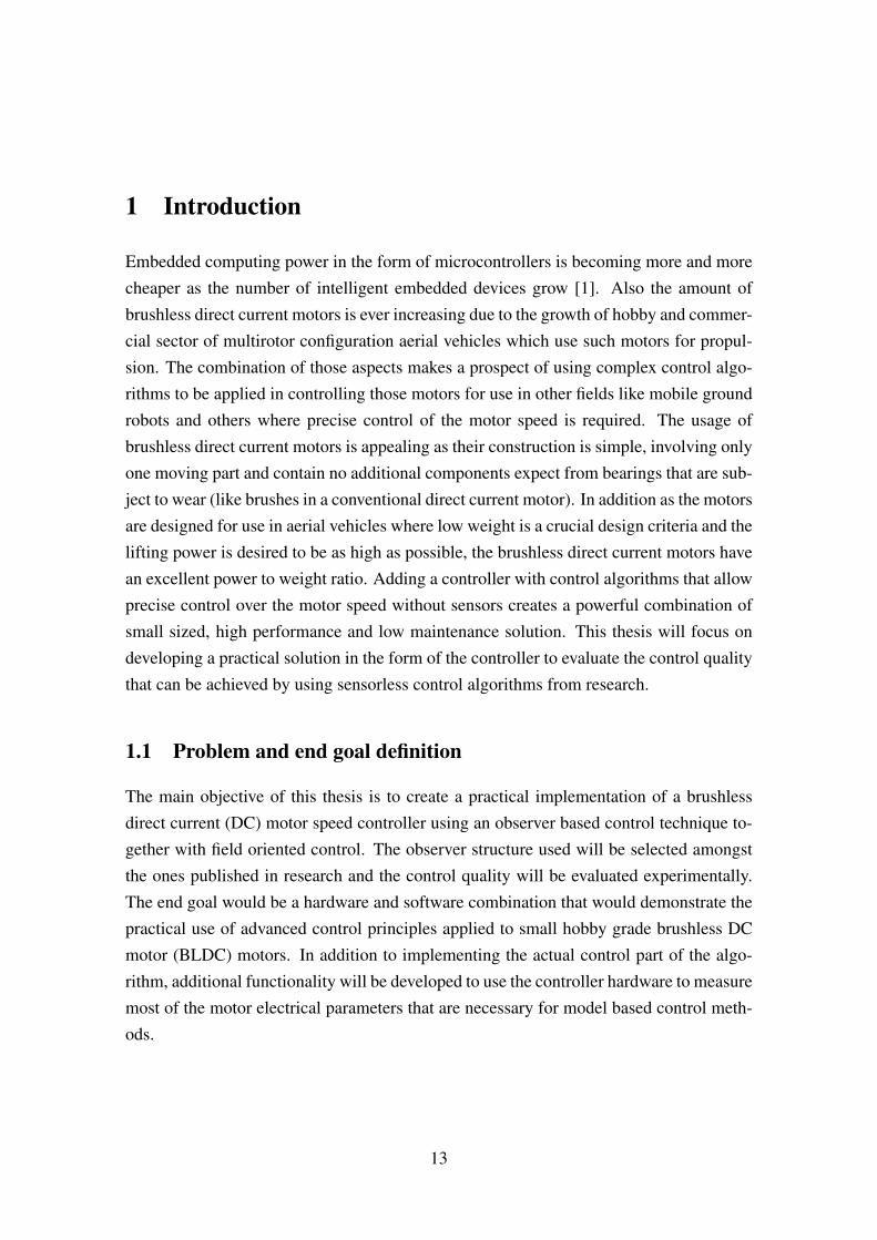
Embedded computing power in the form of microcontrollers is becoming more and morecheaper as the number of intelligent embedded devices grow [1]. Also the amount ofbrushless direct current motors is ever increasing due to the growth of hobby and commer-cial sector of multirotor configuration aerial vehicles which use such motors for propul-sion. The combination of those aspects makes a prospect of using complex control algo-rithms to be applied in controlling those motors for use in other fields like mobile groundrobots and others where precise control of the motor speed is required. The usage ofbrushless direct current motors is appealing as their construction is simple, involving onlyone moving part and contain no additional components expect from bearings that are sub-ject to wear (like brushes in a conventional direct current motor). In addition as the motorsare designed for use in aerial vehicles where low weight is a crucial design criteria and thelifting power is desired to be as high as possible, the brushless direct current motors havean excellent power to weight ratio. Adding a controller with control algorithms that allowprecise control over the motor speed without sensors creates a powerful combination ofsmall sized, high performance and low maintenance solution. This thesis will focus ondeveloping a practical solution in the form of the controller to evaluate the control qualitythat can be achieved by using sensorless control algorithms from research.
1.1 Problem and end goal definition
The main objective of this thesis is to create a practical implementation of a brushlessdirect current (DC) motor speed controller using an observer based control technique to-gether with field oriented control. The observer structure used will be selected amongstthe ones published in research and the control quality will be evaluated experimentally.The end goal would be a hardware and software combination that would demonstrate thepractical use of advanced control principles applied to small hobby grade brushless DCmotor (BLDC) motors. In addition to implementing the actual control part of the algo-rithm, additional functionality will be developed to use the controller hardware to measuremost of the motor electrical parameters that are necessary for model based control meth-ods.
13
1.2 Methodology
At first a theoretical introduction to synchronous alternating current motors, control meth-ods and observe based control is given. Then an overview of the designed hardware willbe given with the working principles of the parts essential to the control algorithm imple-mentation.
The practical algorithm implementation part will be divided into two. The first part willconcentrate on the motor parameter measurement methods to allow model based controlapproaches to be implemented. It will consist of motor electrical parameter measurementalgorithms so that minimal amount of external information would be needed by the con-troller to successfully perform the control tasks. In the second part an observer structure isselected from the available research done in the field and implemented on the microcon-troller. In addition to the pure implementation of the observer, practical implementationproblems will be resolved so that the result will be a fully functional speed control ap-proach to brushless DC motors.
Lastly the performance of the final controller will be evaluated against the requirementsand conclusions are made about the observer operation and control quality achieved.
The controller hardware design was done using Altium Designer software suite, whichis a professional printed circuit board schematic and layout software. The source codewas created using Visual Studio 2017 and VisualGDB extension from Sysprogs OÜ. Theflashing and debugging was done using Lauterbach PowerDebug II and PowerTrace IIadapters and accompanying Trace32 software, which enabled a lot more insight into therun-time code execution and helped to solve a lot of problems related to interrupt anddirect-memory access functionality very quickly.
14
2 Theoretical overview
This section gives a general overview of three phase motors and how used brushless directcurrent DC motors are situated amongst them. Then an overview of three phase motorcontrol methods is given, with focus on field oriented control and space vector modula-tion. Lastly an introduction to observer based control is made and an overview of state ofthe art observer based control of synchronous three phase motors is given.
2.1 Three phase synchronous motors
Three phase synchronous motors are a form of alternating current motors, where the sta-tionary part of the motor consists of field windings and the rotating part of the motor iscomposed of permanent magnets that rotate in the magnetic field created by stator wind-ings when an appropriate three phase current is applied. Synchronous motors operate ata constant speed with absolute synchronism with the input current frequency. The ab-solute synchronism means, that the input alternating current creates a rotating magneticfield by the stator windings. The permanent magnets mounted on the rotor will followthat rotating field precisely, given that the magnetic field created by the stator is strongenough.Synchronous motors are classified according to their rotor design, constructionand operation into four groups [2]:
electromagnetically-excited motors
permanent magnet motors
reluctance motors
hysteresis motors
Brushless DC motors are classified as a type of permanent magnet synchronous mo-tors. The notion of being a DC motor comes from the fact that these types of motorsare typically driven using rectangular current pulses, even though they are AC motors[3]. The difference from conventional permanent magnet synchronous motors (PMSM)comes from the shape of the electromotive force generated by the motor. Usually it’s beenthe way that BLDC motors have trapezoidal shaped back-EMF waveform and PM syn-chronous motors have sinusoidal back-electromotive force electromotive force (EMF) [3].In this thesis BLDC motors are considered as general alternating current (AC) machines
15
that are driven with three phase alternating currents.
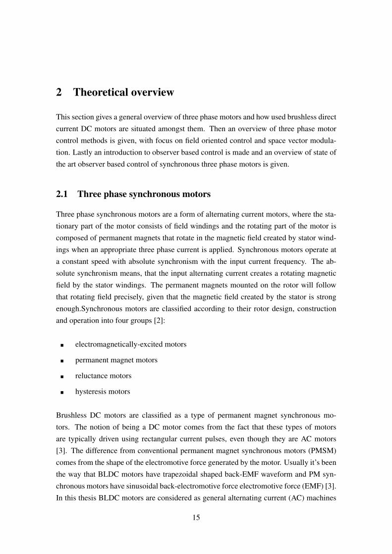
BLDC motors can have different configurations regarding the construction. A commonaspect between those configurations is that the permanent magnets are mounted on therotor and the field windings are contained in the stator. There exists two main configu-rations that BLDC motors are produced: inrunner configuration where the rotor residesinside the stator and outrunner configuration where the stator is inside the rotor. Themotors used in this work are of outrunner type with permanent magnets mounted to thesurface of the rotor, classifying them as surface-permanent magnet motors (SPMSM) andsuch configuration is visible in figure 1. The aspect that magnets are mounted on the sur-face of the rotor define an important property of the motor that will reduce the complexityof control implementation. Motor with magnets on the surface of the rotor are consideredto be magnetically round (non-salient). This implies that the inductances in the directand quadrature axes will be equal so we can consider that Ld = Lq = Ls. Synchronousmotor with permanent magnet mounted on the surface of the rotor can be described bythe following equations from [4]:
Figure 1. BLDC motor with outside rotor [3].
Classical mathematical model of a surface-PMSM motor in the stator fixed referenceframe is the following [5]:
Ls ·diαβ
dt=−Rs · iαβ −ω ·λ ·
−sin(θ)
cos(θ)
+uαβ
θ = np ·ω
(1)
where Ls is the stator inductance, iαβ = [iα iβ ]T stator currents in the stationary reference
16
frame, Rs resistance of stator phase winding, ω electrical angular velocity, λ flux linkage,uαβ = [uα uβ ]
T stator voltages in the stationary reference frame and np is the number ofpole pairs the motor has.
Electrical torque produced by the motor is given by
Te = Kt · (iβ · cos(θ)− iα · sin(θ)) (2)
where Kt is the torque constant of the motor given by
Kt =32·λ ·np (3)
As can be seen from equation (1) the mathematical model has three constant parameters:stator winding resistance Rs, stator winding inductance Ls and the flux linkage λm. Theseare the parameters that are necessary to measure for a specific motor to implement a modelbased control approach such as observer based control.
2.2 Main control principles
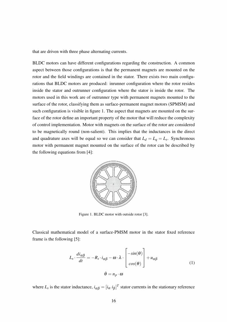
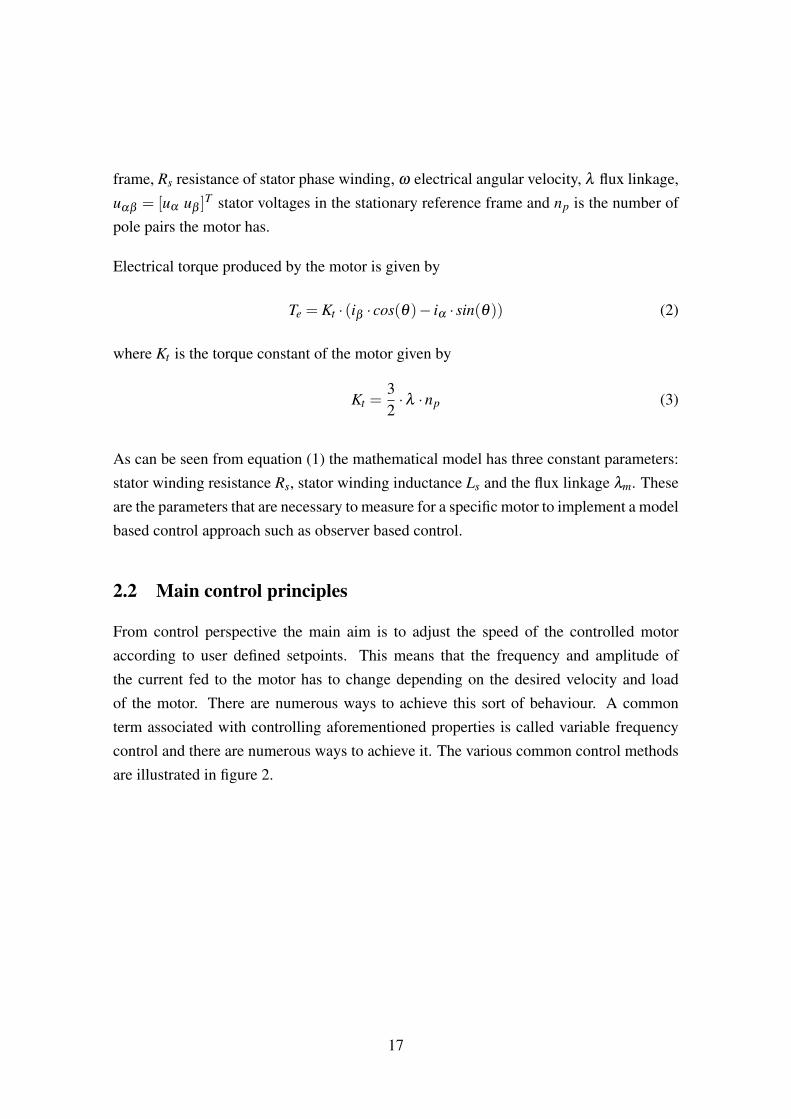
From control perspective the main aim is to adjust the speed of the controlled motoraccording to user defined setpoints. This means that the frequency and amplitude ofthe current fed to the motor has to change depending on the desired velocity and loadof the motor. There are numerous ways to achieve this sort of behaviour. A commonterm associated with controlling aforementioned properties is called variable frequencycontrol and there are numerous ways to achieve it. The various common control methodsare illustrated in figure 2.
17
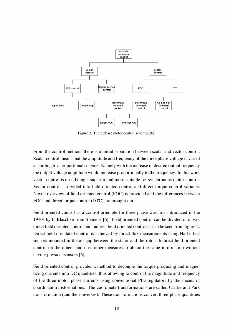
Figure 2. Three phase motor control schemes [6].
From the control methods there is a initial separation between scalar and vector control.Scalar control means that the amplitude and frequency of the three phase voltage is variedaccording to a proportional scheme. Namely with the increase of desired output frequencythe output voltage amplitude would increase proportionally to the frequency. In this workvector control is used being a superior and more suitable for synchronous motor control.Vector control is divided into field oriented control and direct torque control variants.Next a overview of field oriented control (FOC) is provided and the differences betweenFOC and direct torque control (DTC) are brought out.
Field oriented control as a control principle for three phase was first introduced in the1970s by F. Blaschke from Siemens [6]. Field oriented control can be divided into two:direct field oriented control and indirect field oriented control as can be seen from figure 2.Direct field orientated control is achieved by direct flux measurements using Hall effectsensors mounted in the air-gap between the stator and the rotor. Indirect field orientedcontrol on the other hand uses other measures to obtain the same information withouthaving physical sensors [6].
Field oriented control provides a method to decouple the torque producing and magne-tizing currents into DC quantities, thus allowing to control the magnitude and frequencyof the three motor phase currents using conventional PID regulators by the means ofcoordinate transformations. The coordinate transformations are called Clarke and Parktransformation (and their inverses). These transformations convert three-phase quantities
18
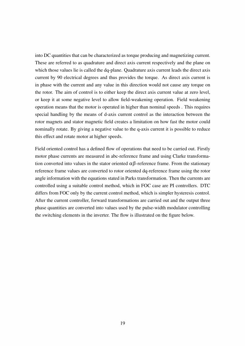
into DC quantities that can be characterized as torque producing and magnetizing current.These are referred to as quadrature and direct axis current respectively and the plane onwhich those values lie is called the dq-plane. Quadrature axis current leads the direct axiscurrent by 90 electrical degrees and thus provides the torque. As direct axis current isin phase with the current and any value in this direction would not cause any torque onthe rotor. The aim of control is to either keep the direct axis current value at zero level,or keep it at some negative level to allow field-weakening operation. Field weakeningoperation means that the motor is operated in higher than nominal speeds . This requiresspecial handling by the means of d-axis current control as the interaction between therotor magnets and stator magnetic field creates a limitation on how fast the motor couldnominally rotate. By giving a negative value to the q-axis current it is possible to reducethis effect and rotate motor at higher speeds.
Field oriented control has a defined flow of operations that need to be carried out. Firstlymotor phase currents are measured in abc-reference frame and using Clarke transforma-tion converted into values in the stator oriented αβ -reference frame. From the stationaryreference frame values are converted to rotor oriented dq-reference frame using the rotorangle information with the equations stated in Parks transformation. Then the currents arecontrolled using a suitable control method, which in FOC case are PI controllers. DTCdiffers from FOC only by the current control method, which is simpler hysteresis control.After the current controller, forward transformations are carried out and the output threephase quantities are converted into values used by the pulse-width modulator controllingthe switching elements in the inverter. The flow is illustrated on the figure below.
19
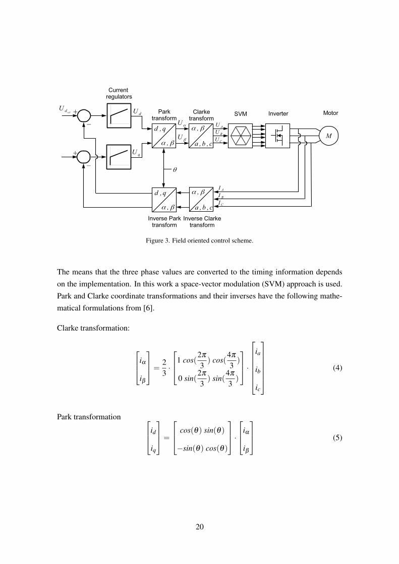
Figure 3. Field oriented control scheme.
The means that the three phase values are converted to the timing information dependson the implementation. In this work a space-vector modulation (SVM) approach is used.Park and Clarke coordinate transformations and their inverses have the following mathe-matical formulations from [6].
Clarke transformation:
iα
iβ
=23·
1 cos(2π
3) cos(
4π
3)
0 sin(2π
3) sin(
4π
3)
·
ia
ib
ic
(4)
Park transformation id
iq
=
cos(θ) sin(θ)
−sin(θ) cos(θ)
·iα
iβ
(5)
20
Inverse Clarke transformation:Ua
Ub
Uc
=
Uα
−12·Uα +
√3
2·Uβ
−12·Uα −
√3
2·Uβ
(6)
Inverse Park transformation:Uα
Uβ
=
cos(θ) − sin(θ)
sin(θ) cos(θ)
·Ud
Uq
(7)
2.3 Three phase inverters
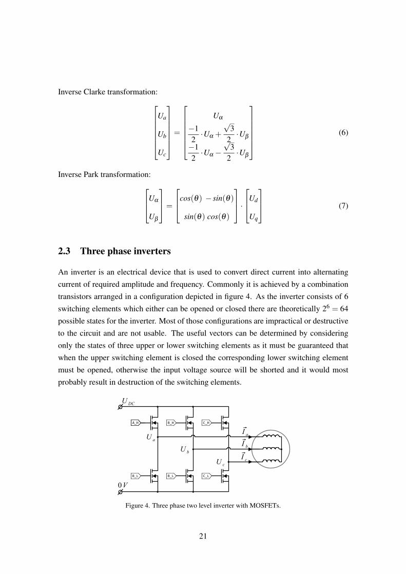
An inverter is an electrical device that is used to convert direct current into alternatingcurrent of required amplitude and frequency. Commonly it is achieved by a combinationtransistors arranged in a configuration depicted in figure 4. As the inverter consists of 6switching elements which either can be opened or closed there are theoretically 26 = 64possible states for the inverter. Most of those configurations are impractical or destructiveto the circuit and are not usable. The useful vectors can be determined by consideringonly the states of three upper or lower switching elements as it must be guaranteed thatwhen the upper switching element is closed the corresponding lower switching elementmust be opened, otherwise the input voltage source will be shorted and it would mostprobably result in destruction of the switching elements.
Figure 4. Three phase two level inverter with MOSFETs.
21
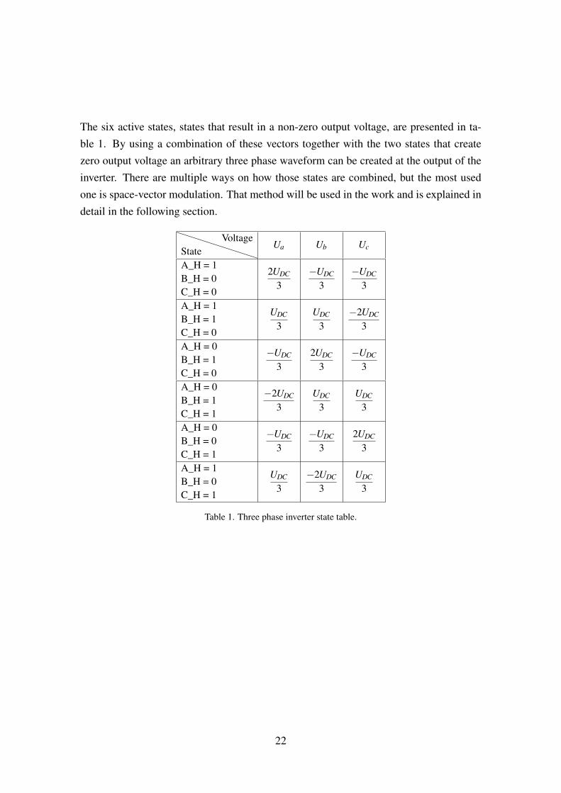
The six active states, states that result in a non-zero output voltage, are presented in ta-ble 1. By using a combination of these vectors together with the two states that createzero output voltage an arbitrary three phase waveform can be created at the output of theinverter. There are multiple ways on how those states are combined, but the most usedone is space-vector modulation. That method will be used in the work and is explained indetail in the following section.
StateVoltage
Ua Ub Uc
A_H = 1B_H = 0C_H = 0
2UDC
3−UDC
3−UDC
3
A_H = 1B_H = 1C_H = 0
UDC
3UDC
3−2UDC
3
A_H = 0B_H = 1C_H = 0
−UDC
32UDC
3−UDC
3
A_H = 0B_H = 1C_H = 1
−2UDC
3UDC
3UDC
3
A_H = 0B_H = 0C_H = 1
−UDC
3−UDC
32UDC
3
A_H = 1B_H = 0C_H = 1
UDC
3−2UDC
3UDC
3
Table 1. Three phase inverter state table.
22
2.4 Space-vector modulation
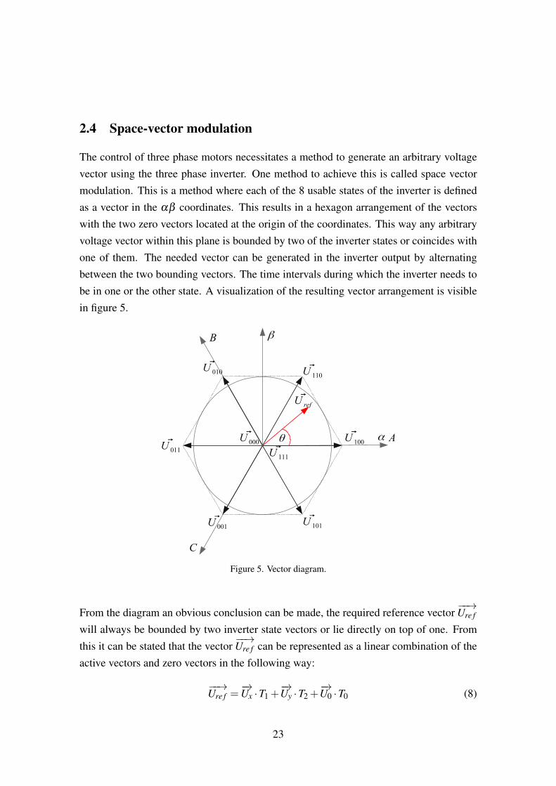
The control of three phase motors necessitates a method to generate an arbitrary voltagevector using the three phase inverter. One method to achieve this is called space vectormodulation. This is a method where each of the 8 usable states of the inverter is definedas a vector in the αβ coordinates. This results in a hexagon arrangement of the vectorswith the two zero vectors located at the origin of the coordinates. This way any arbitraryvoltage vector within this plane is bounded by two of the inverter states or coincides withone of them. The needed vector can be generated in the inverter output by alternatingbetween the two bounding vectors. The time intervals during which the inverter needs tobe in one or the other state. A visualization of the resulting vector arrangement is visiblein figure 5.
Figure 5. Vector diagram.
From the diagram an obvious conclusion can be made, the required reference vector−−→Ure f
will always be bounded by two inverter state vectors or lie directly on top of one. Fromthis it can be stated that the vector
−−→Ure f can be represented as a linear combination of the
active vectors and zero vectors in the following way:
−−→Ure f =
−→Ux ·T1 +
−→Uy ·T2 +
−→U0 ·T0 (8)
23
The vectors−→Ux and
−→Uy represent the vectors bounding the reference vector
−−→Ure f . Values
T1, T2 and T0 are the time amounts determining on how long the inverter needs to be instates defined by vector
−→Ux and
−→Uy respectively. The calculation of those time instances is
the following, assuming that T is the switching period of the inverter and θ is the anglebetween reference vector and inverter state vector
−−→U100:
T1 = T ·∥∥∥∥−−→Ure f
∥∥∥∥ · sin(60−θ)
T2 = T ·∥∥∥∥−−→Ure f
∥∥∥∥ · sin(θ)
T0 = T −T1−T2
(9)
On the diagram an overlay of two different coordinate frames has been added to demon-strate how the input to the modulator can be either in abc-reference frame or the αβ
reference frame.
2.5 Observer based control
A state observer is a dynamic system which estimates the state variables based on themeasurements of the systems output and control variables [7]. Observer is a subsystemthat allows the reconstruction of the state of the plant. Observers are used to solve controltasks when the states of the system are not directly measurable but can be obtained fromindirect measurements and the model of the plant. Mathematically a plant can be definedby the following equations [7]:
x = Ax+Bu
y =Cx(10)
24
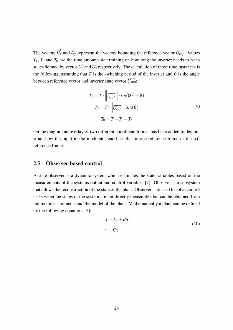
Figure 6. Principle of observer based control.
In observer based control approach the controller takes a time-varying input of the desiredsystem output yd(t) and transforms this to a suitable control signal u(t), where the feed-back loop is completed by the state estimate x from the state observer. It is the observersrole to take the controller generated control signal and real system output y(t) to computethe estimate of the systems state based on the mathematical model of the plant and a suit-able function that would minimize the difference between the observers estimate and thetrue system state. Mathematically the model of the observer is the following [7]:
˙x = Ax+Bu+Ke(y−Cx) (11)
In order to implement observer based control the plant has to be observable. It is said,that the system can be completely observed, if every state can be determined from theobservation of system output y(t) over time [7].
2.5.1 State of the art
Latest research in observer based sensorless control of permanent magnet motor dividesthe control approach to two distinct variants: high frequency injection methods [8], [9]and model based estimation methods [10],[11],[12]. Model based approaches focus pre-dominantly on observer based solutions, split into two main directions based on the sys-tem states observes: estimation of back-EMF or flux (either stator or rotor). Most of theimplementations use a sliding-mode observer structure to estimate the aforementionedstates of the system to derive the rotor electrical angle. In [10] and adaptive frequencytracking mode observer approach is proposed to track the fundamental wave of the sta-
25
tor currents, from which the back-EMF signal is estimated. Sliding mode observer angleestimation accuracy improvements with neural networks is presented in [11]. There theobserver output error is fed into an (ADALINE) neural network to filter the ripples presentin the estimation error. In addition to sliding mode observer based control, conventionalnonlinear observers are in the focus of research for estimating the rotor position withoutsensors. In [12] a nonlinear flux observer together with PLL as a method to obtain angu-lar velocity information from position information , with equivalent observer equations asused in this thesis, is presented.
26
3 Hardware overview
This chapter describes the designed hardware for controlling BLDC motors. It covers themain components: microcontroller, inverter and current sensing parts with their selectioncriteria and the operating principle. Lastly information about the selected motors and thefinal experimental setup is given. All the schematics of the designed board are presentedin Appendix 1 –.
3.1 Motor controller
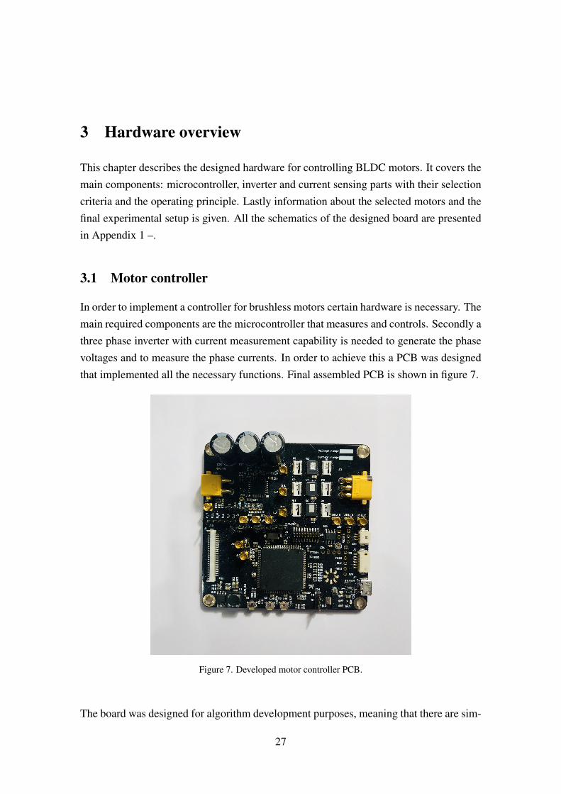
In order to implement a controller for brushless motors certain hardware is necessary. Themain required components are the microcontroller that measures and controls. Secondly athree phase inverter with current measurement capability is needed to generate the phasevoltages and to measure the phase currents. In order to achieve this a PCB was designedthat implemented all the necessary functions. Final assembled PCB is shown in figure 7.
Figure 7. Developed motor controller PCB.
The board was designed for algorithm development purposes, meaning that there are sim-
27
iliar or redundant functionality in the current sensing, and most importantly many of thecritical signals have been made accessible for external probing to simplify the verificationof algorithms functionality.
3.1.1 Microcontroller
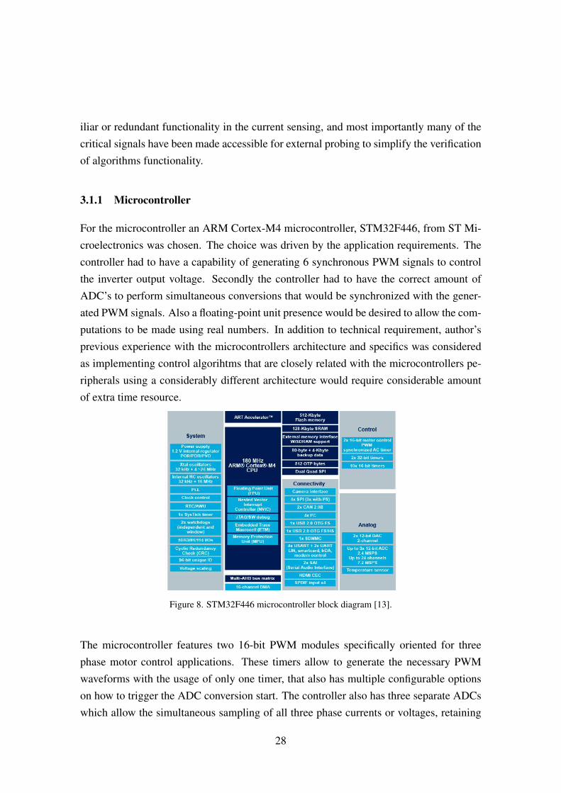
For the microcontroller an ARM Cortex-M4 microcontroller, STM32F446, from ST Mi-croelectronics was chosen. The choice was driven by the application requirements. Thecontroller had to have a capability of generating 6 synchronous PWM signals to controlthe inverter output voltage. Secondly the controller had to have the correct amount ofADC’s to perform simultaneous conversions that would be synchronized with the gener-ated PWM signals. Also a floating-point unit presence would be desired to allow the com-putations to be made using real numbers. In addition to technical requirement, author’sprevious experience with the microcontrollers architecture and specifics was consideredas implementing control algorihtms that are closely related with the microcontrollers pe-ripherals using a considerably different architecture would require considerable amountof extra time resource.
Figure 8. STM32F446 microcontroller block diagram [13].
The microcontroller features two 16-bit PWM modules specifically oriented for threephase motor control applications. These timers allow to generate the necessary PWMwaveforms with the usage of only one timer, that also has multiple configurable optionson how to trigger the ADC conversion start. The controller also has three separate ADCswhich allow the simultaneous sampling of all three phase currents or voltages, retaining
28
the phase characteristics of the original signals, reducing the algorithms complexity asotherwise the non-simultaneous measurements should be compensated in software
3.1.2 Three phase inverter and gate driver
Inverter circuit for the PCB was designed to use metal–oxide–semiconductor field-effect transistor (MOSFET) type transistors as switching elements. SpecificallyCSD88599Q5DC dual MOSFET from Texas Instruments was selected. The device al-ready consists of two transistors in a suitable configuration, thus reducing the overallboard area required by the switching elements and reducing the routing complexity of thePCB.
To control the gates of an inverter consisting only N-type MOSFETs a gate driver is nec-cessary. For this purpose an intelligent gate driver IC DRV8305 from Texas instrumentswas chosen. The IC contains numerous other functionality that reduce the design com-plexity. Namely it has three current shunt amplifiers to convert the measured voltagedrop across the shunt resistor to a suitable range for the microcontrollers ADC, variousconfigurable methods to protect the power transistors and other functionality.
3.1.3 Phase current sensing
Phase current measurement is one of the critical parts of the system which must operatecorrectly and precisely in order for the algorithms depending on it to work correctly. Thereare two main methods for sensing the current in three phase inverters: low-side currentsensing and in-line current sensing.
Low side current sensing means that the current is measured using shunt resistors that areconnected between the electrical ground of the system and the low-side inverter switchingelements. This solution is cheap as the operational amplifiers necessary to amplify thevoltage drop across the shunt resistor are more lenient in their parameters. The maindownside of this configuration is that the current measurement is valid only when thelow-side inverter switch is closed, allowing the current pass through the shunt resistor.This means that software methods have to be applied to ensure that the ADCs measuringthe shunt amplifiers output voltage are triggered at the correct time instant.
In line current sensing means that the shunt resistors are connected in line with the load
29
phases. The main advantage of this configuration is that the current measurements arealways valid, reducing the software complexity associated with ADC triggering. Thedownside is that the current sense amplifiers need to conform to more stringent specifica-tions making them more expensive.
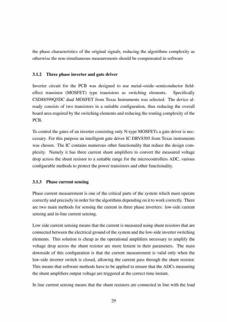
For this controller board both versions were implemented as this board was intended onlyfor research properties, having both options would widen the number of control methodsthat can be experimented with. In the final implementation, low-side current sensingapproach was used. The block diagram of the sense amplifier used inside the gate driveris the following:
Figure 9. Current sense amplifier within DRV8305 IC [14].
Another important aspect is calibration of the current measurement to precisely measurethe instantaneous current value through each motor phase. Calibration procedure involvessourcing the current through the three phase inverter and recording the measured ADCreadings with current measurements by a multimeter. From the measurement points itis possible to construct equations by the means of regression analysis. The resultingequations will allow to correct for the zero offset errors - difference between zero currentand actual ADC reading and the slope of the value, given the assumption from Ohm’s lawthat voltage drop across a resistor is proportional to the current passing through it.
30
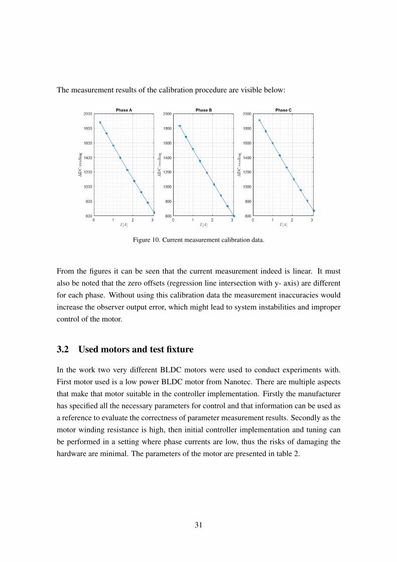
The measurement results of the calibration procedure are visible below:
Figure 10. Current measurement calibration data.
From the figures it can be seen that the current measurement indeed is linear. It mustalso be noted that the zero offsets (regression line intersection with y- axis) are differentfor each phase. Without using this calibration data the measurement inaccuracies wouldincrease the observer output error, which might lead to system instabilities and impropercontrol of the motor.
3.2 Used motors and test fixture
In the work two very different BLDC motors were used to conduct experiments with.First motor used is a low power BLDC motor from Nanotec. There are multiple aspectsthat make that motor suitable in the controller implementation. Firstly the manufacturerhas specified all the necessary parameters for control and that information can be used asa reference to evaluate the correctness of parameter measurement results. Secondly as themotor winding resistance is high, then initial controller implementation and tuning canbe performed in a setting where phase currents are low, thus the risks of damaging thehardware are minimal. The parameters of the motor are presented in table 2.
31
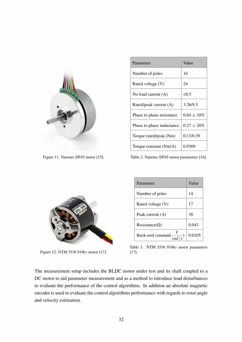
Figure 11. Nanotec DF45 motor [15].
Parameter Value
Number of poles 16
Rated voltage (V) 24
No load current (A) <0.5
Rated/peak current (A) 3.26/9.5
Phase to phase resistance 0.64 ± 10%
Phase to phase inductance 0.27 ± 20%
Torque rated/peak (Nm) 0.13/0.39
Torque constant (Nm/A) 0.0369
Table 2. Nanotec DF45 motor parameters [16].
Figure 12. NTM 3536 910kv motor [17].
Parameter Value
Number of poles 14
Rated voltage (V) 17
Peak current (A) 38
Resistance(Ω) 0.043
Back-emf constant(V
rad/s) 0.0105
Table 3. NTM 3536 910kv motor parameters[17].
The measurement setup includes the BLDC motor under test and its shaft coupled to aDC motor to aid parameter measurement and as a method to introduce load disturbancesto evaluate the performance of the control algorithms. In addition an absolute magneticencoder is used to evaluate the control algorithms performance with regards to rotor angleand velocity estimation.
32
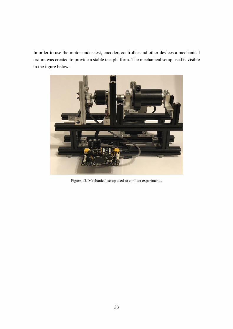
In order to use the motor under test, encoder, controller and other devices a mechanicalfixture was created to provide a stable test platform. The mechanical setup used is visiblein the figure below.
Figure 13. Mechanical setup used to conduct experiments.
33
4 Motor parameter measurement
This chapter describes the measurement procedures and the measurement results of es-sential three phase motor parameters that are necessary by the control algorithms. Themain idea of the measurements is to utilize the capabilities of the developed controller tomeasure the parameters automatically without using other measurement equipment.
All the measurements are verified against a test motor, which has parameters determinedby the manufacturer and allows to evaluate the correctness of measurement methods.
4.1 Stator phase resistance
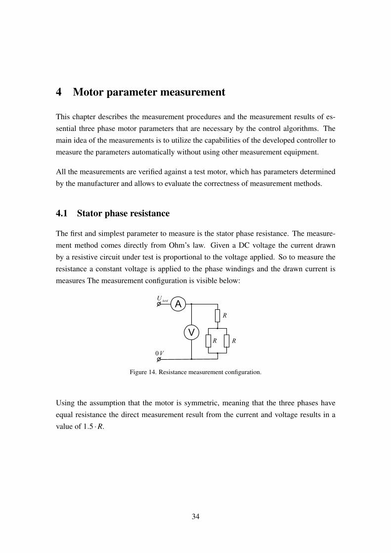
The first and simplest parameter to measure is the stator phase resistance. The measure-ment method comes directly from Ohm’s law. Given a DC voltage the current drawnby a resistive circuit under test is proportional to the voltage applied. So to measure theresistance a constant voltage is applied to the phase windings and the drawn current ismeasures The measurement configuration is visible below:
Figure 14. Resistance measurement configuration.
Using the assumption that the motor is symmetric, meaning that the three phases haveequal resistance the direct measurement result from the current and voltage results in avalue of 1.5 ·R.
34
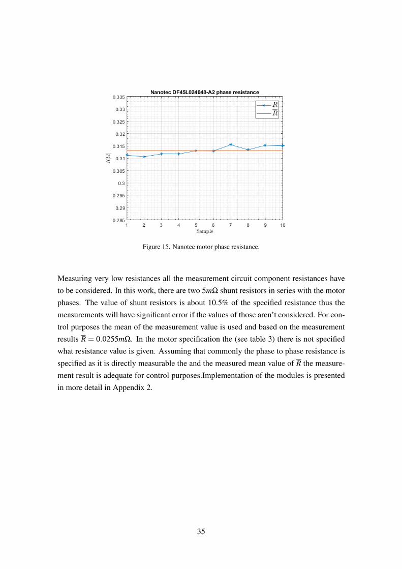
Figure 15. Nanotec motor phase resistance.
Measuring very low resistances all the measurement circuit component resistances haveto be considered. In this work, there are two 5mΩ shunt resistors in series with the motorphases. The value of shunt resistors is about 10.5% of the specified resistance thus themeasurements will have significant error if the values of those aren’t considered. For con-trol purposes the mean of the measurement value is used and based on the measurementresults R = 0.0255mΩ. In the motor specification the (see table 3) there is not specifiedwhat resistance value is given. Assuming that commonly the phase to phase resistance isspecified as it is directly measurable the and the measured mean value of R the measure-ment result is adequate for control purposes.Implementation of the modules is presentedin more detail in Appendix 2.
35
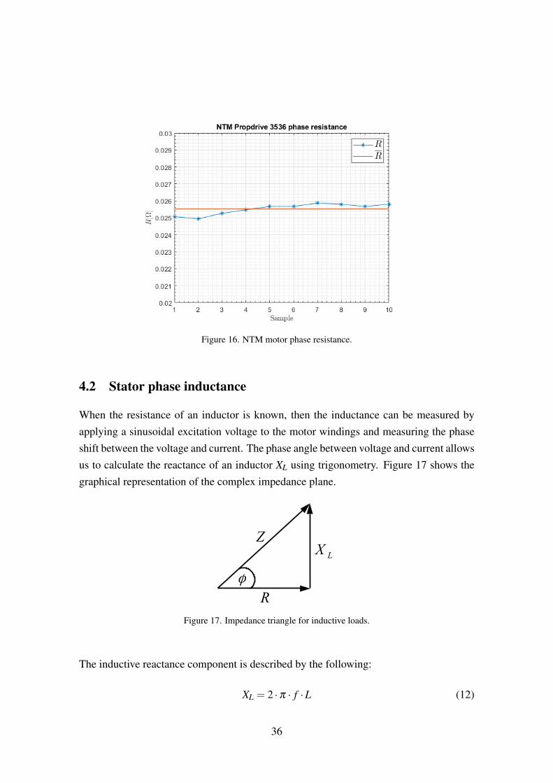
Figure 16. NTM motor phase resistance.
4.2 Stator phase inductance
When the resistance of an inductor is known, then the inductance can be measured byapplying a sinusoidal excitation voltage to the motor windings and measuring the phaseshift between the voltage and current. The phase angle between voltage and current allowsus to calculate the reactance of an inductor XL using trigonometry. Figure 17 shows thegraphical representation of the complex impedance plane.
Figure 17. Impedance triangle for inductive loads.
The inductive reactance component is described by the following:
XL = 2 ·π · f ·L (12)
36
Combining the knowledge of the inductive reactance component and the relationship withthe complex impedance, resistance we can derive the following equation to calculate in-ductance from known resistance R, frequency f and measured phase shift between currentand voltage Φ:
L =R · tan(Φ)
2 ·π · f(13)
To implement the inductance measurement with motor connected to the designed con-troller two software components need to be developed. Firstly a sinusoidal excitation volt-age generator with predefined amplitude and frequency and a method to measure phaseshift between the generated voltage and measured current. The latter was implementedusing a zero crossing detector, which records time instances when voltage and currentvalues change from positive to negative and vice versa. The timestamps are then used tocalculate the frequency of the signals and phase shift between them. Implementation ofthe modules is presented in more detail in Appendix 3.
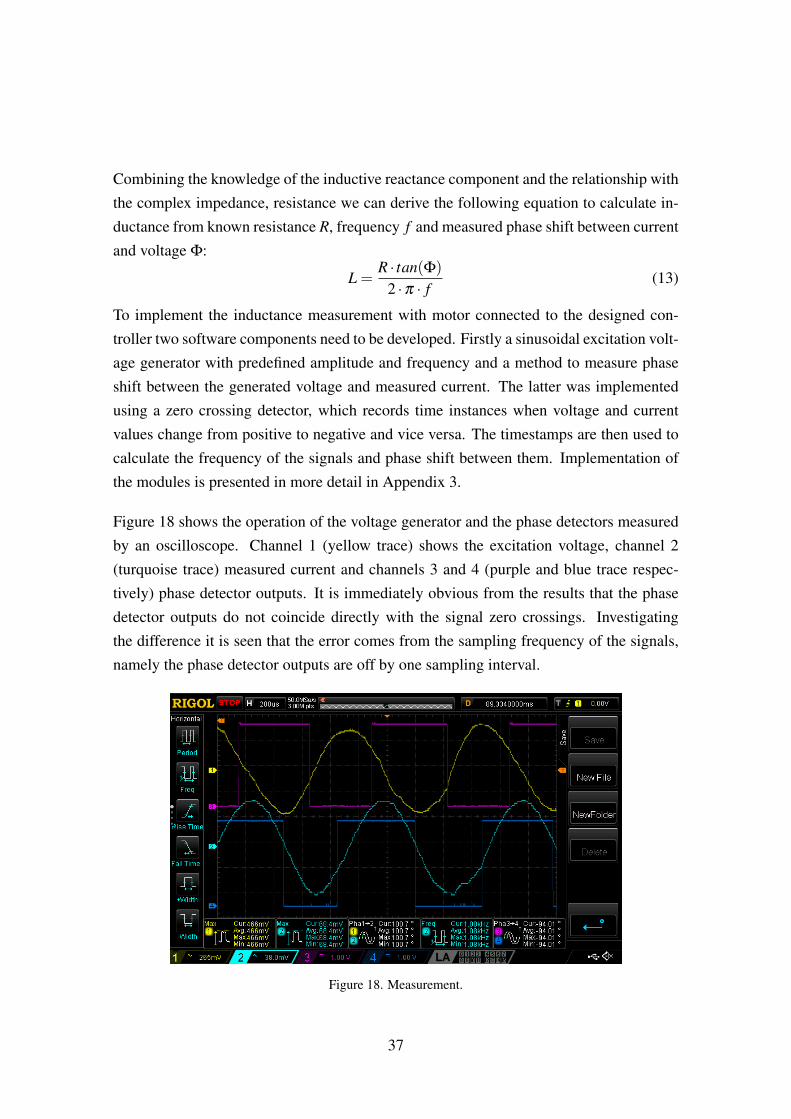
Figure 18 shows the operation of the voltage generator and the phase detectors measuredby an oscilloscope. Channel 1 (yellow trace) shows the excitation voltage, channel 2(turquoise trace) measured current and channels 3 and 4 (purple and blue trace respec-tively) phase detector outputs. It is immediately obvious from the results that the phasedetector outputs do not coincide directly with the signal zero crossings. Investigatingthe difference it is seen that the error comes from the sampling frequency of the signals,namely the phase detector outputs are off by one sampling interval.
Figure 18. Measurement.
37
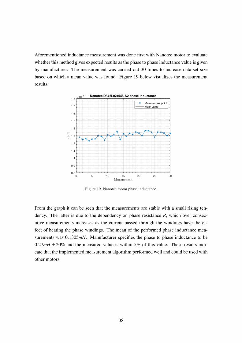
Aforementioned inductance measurement was done first with Nanotec motor to evaluatewhether this method gives expected results as the phase to phase inductance value is givenby manufacturer. The measurement was carried out 30 times to increase data-set sizebased on which a mean value was found. Figure 19 below visualizes the measurementresults.
Figure 19. Nanotec motor phase inductance.
From the graph it can be seen that the measurements are stable with a small rising ten-dency. The latter is due to the dependency on phase resistance R, which over consec-utive measurements increases as the current passed through the windings have the ef-fect of heating the phase windings. The mean of the performed phase inductance mea-surements was 0.1305mH. Manufacturer specifies the phase to phase inductance to be0.27mH ± 20% and the measured value is within 5% of this value. These results indi-cate that the implemented measurement algorithm performed well and could be used withother motors.
38
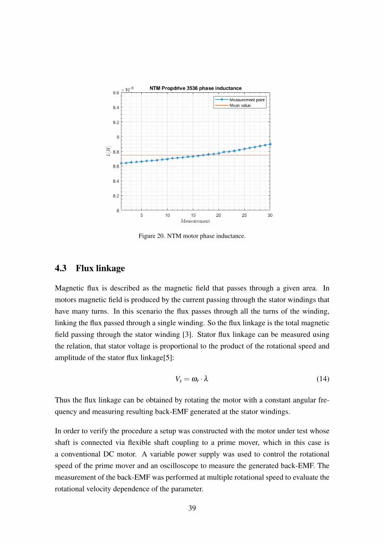
Figure 20. NTM motor phase inductance.
4.3 Flux linkage
Magnetic flux is described as the magnetic field that passes through a given area. Inmotors magnetic field is produced by the current passing through the stator windings thathave many turns. In this scenario the flux passes through all the turns of the winding,linking the flux passed through a single winding. So the flux linkage is the total magneticfield passing through the stator winding [3]. Stator flux linkage can be measured usingthe relation, that stator voltage is proportional to the product of the rotational speed andamplitude of the stator flux linkage[5]:
Vs = ωr ·λ (14)
Thus the flux linkage can be obtained by rotating the motor with a constant angular fre-quency and measuring resulting back-EMF generated at the stator windings.
In order to verify the procedure a setup was constructed with the motor under test whoseshaft is connected via flexible shaft coupling to a prime mover, which in this case isa conventional DC motor. A variable power supply was used to control the rotationalspeed of the prime mover and an oscilloscope to measure the generated back-EMF. Themeasurement of the back-EMF was performed at multiple rotational speed to evaluate therotational velocity dependence of the parameter.
39
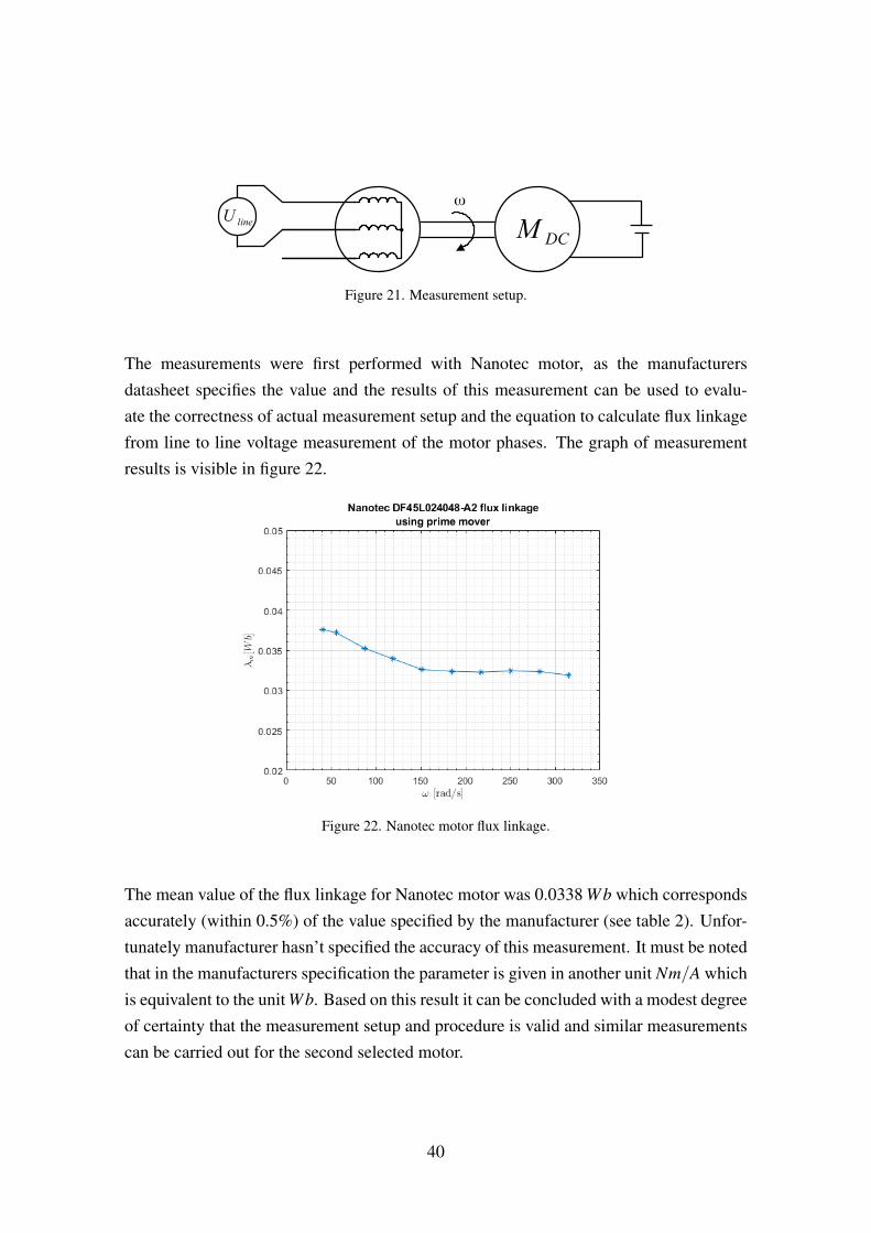
Figure 21. Measurement setup.
The measurements were first performed with Nanotec motor, as the manufacturersdatasheet specifies the value and the results of this measurement can be used to evalu-ate the correctness of actual measurement setup and the equation to calculate flux linkagefrom line to line voltage measurement of the motor phases. The graph of measurementresults is visible in figure 22.
Figure 22. Nanotec motor flux linkage.
The mean value of the flux linkage for Nanotec motor was 0.0338 Wb which correspondsaccurately (within 0.5%) of the value specified by the manufacturer (see table 2). Unfor-tunately manufacturer hasn’t specified the accuracy of this measurement. It must be notedthat in the manufacturers specification the parameter is given in another unit Nm/A whichis equivalent to the unit Wb. Based on this result it can be concluded with a modest degreeof certainty that the measurement setup and procedure is valid and similar measurementscan be carried out for the second selected motor.
40
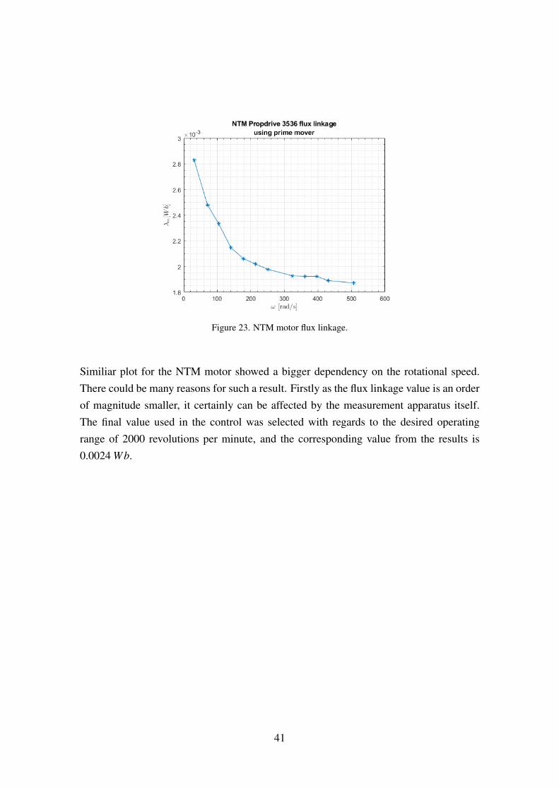
Figure 23. NTM motor flux linkage.
Similiar plot for the NTM motor showed a bigger dependency on the rotational speed.There could be many reasons for such a result. Firstly as the flux linkage value is an orderof magnitude smaller, it certainly can be affected by the measurement apparatus itself.The final value used in the control was selected with regards to the desired operatingrange of 2000 revolutions per minute, and the corresponding value from the results is0.0024 Wb.
41
5 Observer based controller for BLDC motor
This chapter describes the selected observer algorithm used to estimate the rotor electricalangle, its practical implementation with overcoming observer limitations and measure-ment results describing the operational characteristics of the algorithm.
5.1 Controller requirements
For the controller design basic design criteria were fixed. Firstly the controller shall oper-ate reliably from zero speed up to specified velocity setpoint. The speed controller shouldhave regulation. The velocity range at which the controller shall operate is -2000 to 2000revolutions per minute (RPM) performance of ±5%.
5.2 Observer selection
A big multitude of methods exist to estimate the rotor electrical angle only from phasevoltages, currents and motor parameters. For this work a method developed by RomeoOrtega in [18] and explained more in depth by Kwang Hee Nam in [4] was selected.There were multiple reason why to choose this method over other similiar methods. Thealgorithm only considers the electrical model of the motor making it suitable for applica-tion where mechanical parameters like moment of inertia of the motor and load, frictionand other parameters are difficult to obtain. Secondly the observer is designed to workin the stationary αβ reference frame, meaning there is reduced complexity as there is nofeedback from the estimated angular velocity. Also implementations where observer isimplemented in dq reference frame have a major shortcoming, namely any error affectingthe angular position value could invalidate the mathematical model used and consequentlythe resulting design [5]. For the readers convenience the major algorithm derivation partsare reproduced in the next chapter. Chapter 6 describes the practical implementation ofthe algorithm and overcoming the limitations of the selected algorithm in motor start-upand operation through low speed region. Chapter 7 presents the results of the controlleroperation with selected motors.
The novelty of this work comes from applying such type of algorithm on hobby-gradeBLDC motors, which in principle share the same mechanical construction as PMSM mo-tors with surface mounted magnets.
42
5.2.1 Ortega’s observer based angle estimation
PMSM motor with magnets mounted on the surface of the rotor can be mathematicallydescribed in the stationary αβ reference frame as follows:
Ls ·ddt· iα =−Rs · iα +ωλ · sin(θ)+uα
Ls ·ddt· iβ =−Rs · iβ +ωλ · cos(θ)+uβ
(15)
Magnetic flux in the stator Φs is given by the following equation
Φsα= Ls · iα +λ · cos(θ)
Φsβ= Ls · iβ +λ · sin(θ)
(16)
Rotor flux vector Φrα,βthus is the following
Φrα= Φsα
−Ls · iα = λ · cos(θ)
Φrβ= Φsβ
−Ls · iβ = λ · sin(θ)(17)
Equation 17 shows that the rotor electrical angle θ can be obtained from the stator fluxvector in the following manner:
Φsβ−Ls · iβ
Φsα−Ls · iα
=λ · sin(θ)λ · cos(θ)
Φsβ−Ls · iβ
Φsα−Ls · iα
= λ · tanθ
θ = tan−1
(Φsβ−Ls · iβ
Φsα−Ls · iα
) (18)
From 18 we can conclude that the rotor angle θ can be obtained by estimating the statorflux vector Φα,β as the stator inductance Ls is a measurable constant and stator currentvector iα,β is measurable. Using equation 16 we can set the observer state to be thefollowing:
x =
Φsα
Φsα
= Ls ·
iα
iβ
+λ ·
cos(Θ)
sin(Θ)
(19)
43
We can rearrange the observer state equation 21 by moving the term containing Ls to theleft hand side and defining function η(x):
η(x) =
Φsα
Φsα
−Ls ·
iα
iβ
= λ ·
cos(Θ)
sin(Θ)
(20)
Now taking the l2 norm of the matrices, replacing the true stator flux vector with theestimated version ˆΦα,β and squaring the equation sides we can get a suitable error termto correct the observer state: ∥∥∥∥η(x)
∥∥∥∥2
= λ 2
Error = λ 2−∥∥∥∥η(x)
∥∥∥∥2 (21)
Observer proposed in [18] has the following form:
˙x = y+γ
2·η(x) · [λ 2− ‖ η(x) ‖2]
y =−Rs ·
iα
iβ
+uα
uβ
(22)
where γ is the observer gain , η is the defined function in (20), λ is the rotor flux linkage.The
Observer gain selection was performed experimentally. Guidelines for tuning the gain arepresented in [12], where it is suggested that a too high gain value would lead to overesti-mation of the speed but a too low value would not allow the observer to dynamically trackthe speed step reference. These guidelines were used to iteratively tune the observer gainvalue until a satisfying result was found.An optimal value of the gain value γ was foundto be γ = 5000, this value resulted in a good step response tracking with a minor overes-timation of the velocity as shown in chapter 6.3, figure 37, where the speed estimation iscompared with the measured value using an encoder.
44
5.3 Phase-lock loop based velocity calculation
The most common way to obtain velocity information from angular measurements is bythe means of simple differentiation, meaning that the angular velocity value is obtainedusing formula:
ωt =θt−θt−1
dt(23)
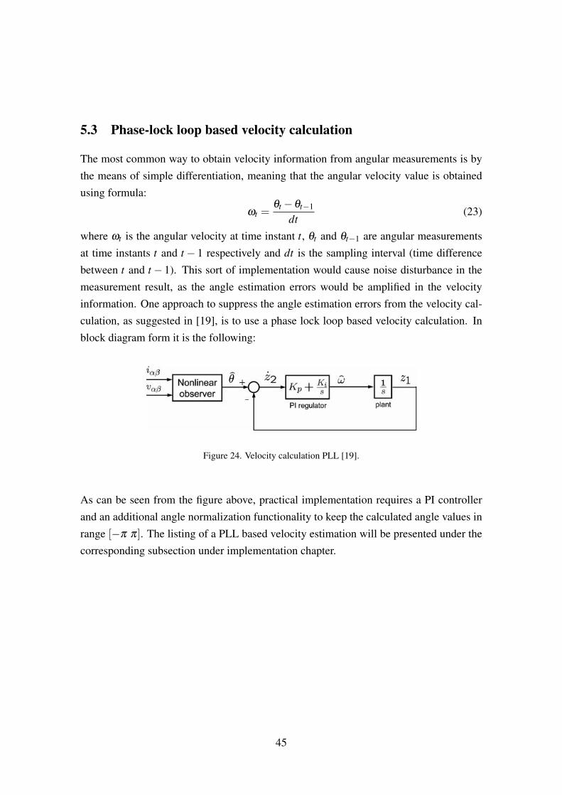
where ωt is the angular velocity at time instant t, θt and θt−1 are angular measurementsat time instants t and t− 1 respectively and dt is the sampling interval (time differencebetween t and t− 1). This sort of implementation would cause noise disturbance in themeasurement result, as the angle estimation errors would be amplified in the velocityinformation. One approach to suppress the angle estimation errors from the velocity cal-culation, as suggested in [19], is to use a phase lock loop based velocity calculation. Inblock diagram form it is the following:
Figure 24. Velocity calculation PLL [19].
As can be seen from the figure above, practical implementation requires a PI controllerand an additional angle normalization functionality to keep the calculated angle values inrange [−π π]. The listing of a PLL based velocity estimation will be presented under thecorresponding subsection under implementation chapter.
45
5.4 Implementation
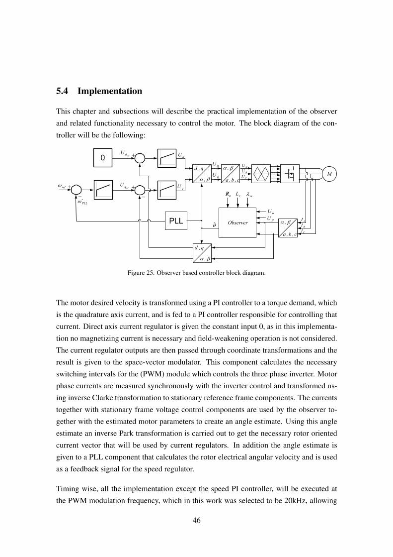
This chapter and subsections will describe the practical implementation of the observerand related functionality necessary to control the motor. The block diagram of the con-troller will be the following:
Figure 25. Observer based controller block diagram.
The motor desired velocity is transformed using a PI controller to a torque demand, whichis the quadrature axis current, and is fed to a PI controller responsible for controlling thatcurrent. Direct axis current regulator is given the constant input 0, as in this implementa-tion no magnetizing current is necessary and field-weakening operation is not considered.The current regulator outputs are then passed through coordinate transformations and theresult is given to the space-vector modulator. This component calculates the necessaryswitching intervals for the (PWM) module which controls the three phase inverter. Motorphase currents are measured synchronously with the inverter control and transformed us-ing inverse Clarke transformation to stationary reference frame components. The currentstogether with stationary frame voltage control components are used by the observer to-gether with the estimated motor parameters to create an angle estimate. Using this angleestimate an inverse Park transformation is carried out to get the necessary rotor orientedcurrent vector that will be used by current regulators. In addition the angle estimate isgiven to a PLL component that calculates the rotor electrical angular velocity and is usedas a feedback signal for the speed regulator.
Timing wise, all the implementation except the speed PI controller, will be executed atthe PWM modulation frequency, which in this work was selected to be 20kHz, allowing
46

quiet operation, but being . The speed PI controller was executed at 1kHz rate as thespeed control loop has mechanical limitations on how big the velocity change betweenexecution intervals could be due to mechanical inertia and friction.
5.4.1 Observer implementation
In order to use the equations derived in [18] program code necessary to implement thefunctionality was written as a function. Observer, as defined in equation 22, implementa-tion as C++ code was the following:
f l o a t FOC : : f O b s e r v e r ( f l o a t d t , f l o a t R , f l o a t L , f l o a t Lm, f l o a t ga in ,Vec_ab_f I , Vec_ab_f U)
f l o a t xa_d , xb_d ; / / O b s e r v e r s t a t e d e r i v a t i v e ss t a t i c f l o a t xa , xb ; / / O b s e r v e r s t a t e sf l o a t e r r o r ; / / O b s e r v e r e r r o rf l o a t t h e t a ; / / E s t i m a t e d r o t o r e l e c t r i c a l a n g l eVec_ab_f LI , RI ; / / V e c t o r s o f L* I and R* I
/ / I n p u t v e c t o r c a l c u l a t i o nLI = I * L ;RI = I * R ;/ / O b s e r v e r e r r o r c a l c u l a t i o ne r r o r = Lm^2 − ( ( xa − LI . a ) ^2 + ( xb − LI . b ) ^2 ) ;/ / S t a t e d e r i v a t i v e sxa_d = −RI . a + U. b + ( g a i n / 2 ) * ( xa − LI . a ) * e r r o r ;xb_d = −RI . b + U. a + ( g a i n / 2 ) * ( xb − LI . b ) * e r r o r ;/ / I n t e g r a t i o n o f s t a t e d e r i v a t i v e sxa += xa_d * d t ;xb += xb_d * d t ;/ / Angle c a l c u l a t i o nt h e t a = a t a n 2 f ( x2 − LI . b , x1 − LI . a ) ;r e t u r n t h e t a ;
Figure 26. Observer implementation.
47
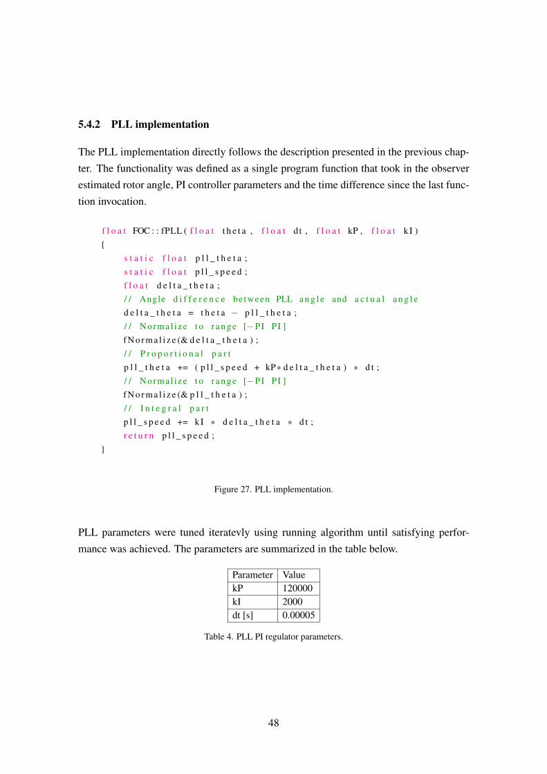
5.4.2 PLL implementation
The PLL implementation directly follows the description presented in the previous chap-ter. The functionality was defined as a single program function that took in the observerestimated rotor angle, PI controller parameters and the time difference since the last func-tion invocation.
f l o a t FOC : : fPLL ( f l o a t t h e t a , f l o a t d t , f l o a t kP , f l o a t k I )
s t a t i c f l o a t p l l _ t h e t a ;s t a t i c f l o a t p l l _ s p e e d ;f l o a t d e l t a _ t h e t a ;/ / Angle d i f f e r e n c e between PLL a n g l e and a c t u a l a n g l ed e l t a _ t h e t a = t h e t a − p l l _ t h e t a ;/ / Normal i ze t o r a n g e [−PI PI ]f N o r m a l i z e (& d e l t a _ t h e t a ) ;/ / P r o p o r t i o n a l p a r tp l l _ t h e t a += ( p l l _ s p e e d + kP* d e l t a _ t h e t a ) * d t ;/ / Normal i ze t o r a n g e [−PI PI ]f N o r m a l i z e (& p l l _ t h e t a ) ;/ / I n t e g r a l p a r tp l l _ s p e e d += kI * d e l t a _ t h e t a * d t ;r e t u r n p l l _ s p e e d ;
Figure 27. PLL implementation.
PLL parameters were tuned iteratevly using running algorithm until satisfying perfor-mance was achieved. The parameters are summarized in the table below.
Parameter ValuekP 120000kI 2000dt [s] 0.00005
Table 4. PLL PI regulator parameters.
48
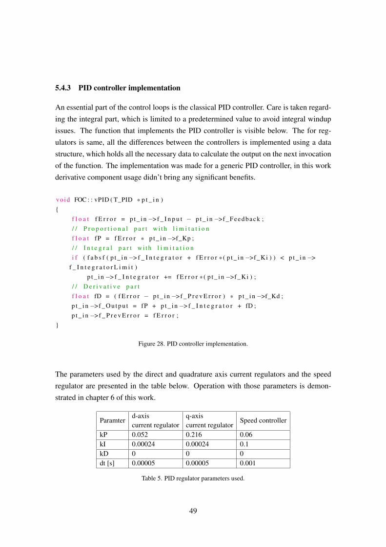
5.4.3 PID controller implementation
An essential part of the control loops is the classical PID controller. Care is taken regard-ing the integral part, which is limited to a predetermined value to avoid integral windupissues. The function that implements the PID controller is visible below. The for reg-ulators is same, all the differences between the controllers is implemented using a datastructure, which holds all the necessary data to calculate the output on the next invocationof the function. The implementation was made for a generic PID controller, in this workderivative component usage didn’t bring any significant benefits.
vo id FOC : : vPID ( T_PID * p t _ i n )
f l o a t f E r r o r = p t _ i n −>f _ I n p u t − p t _ i n −>f_Feedback ;/ / P r o p o r t i o n a l p a r t w i th l i m i t a t i o nf l o a t fP = f E r r o r * p t _ i n −>f_Kp ;/ / I n t e g r a l p a r t w i th l i m i t a t i o ni f ( f a b s f ( p t _ i n −> f _ I n t e g r a t o r + f E r r o r * ( p t _ i n −>f_Ki ) ) < p t _ i n −>
f _ I n t e g r a t o r L i m i t )p t _ i n −> f _ I n t e g r a t o r += f E r r o r * ( p t _ i n −>f_Ki ) ;
/ / D e r i v a t i v e p a r tf l o a t fD = ( f E r r o r − p t _ i n −>f _ P r e v E r r o r ) * p t _ i n −>f_Kd ;p t _ i n −>f _ O u t p u t = fP + p t _ i n −> f _ I n t e g r a t o r + fD ;p t _ i n −>f _ P r e v E r r o r = f E r r o r ;
Figure 28. PID controller implementation.
The parameters used by the direct and quadrature axis current regulators and the speedregulator are presented in the table below. Operation with those parameters is demon-strated in chapter 6 of this work.
Paramterd-axiscurrent regulator
q-axiscurrent regulator
Speed controller
kP 0.052 0.216 0.06kI 0.00024 0.00024 0.1kD 0 0 0dt [s] 0.00005 0.00005 0.001
Table 5. PID regulator parameters used.
49
5.4.4 Motor startup procedure
The observer output is not usable at the low speed region, meaning that using the angleestimated by the observer is not usable below certain threshold. Consequently a methodhas to devised to start the motor without observer and accelerate it above the thresholdspeed. Although not ideal, but a viable method is to start the motor in open-loop scalarcontrol. Meaning that the motor is controlled by a rotating voltage vector where themagnitude and frequency are given without any feedback.The disadvantage of this methodis that the assumption that the motor rotates according to the given rotating voltage vectormight not be true. Namely when the torque produced is insufficient to keep the rotor fluxvector in synchronization with stator flux vector then the motor will just start oscillatingwithin one electrical revolution.
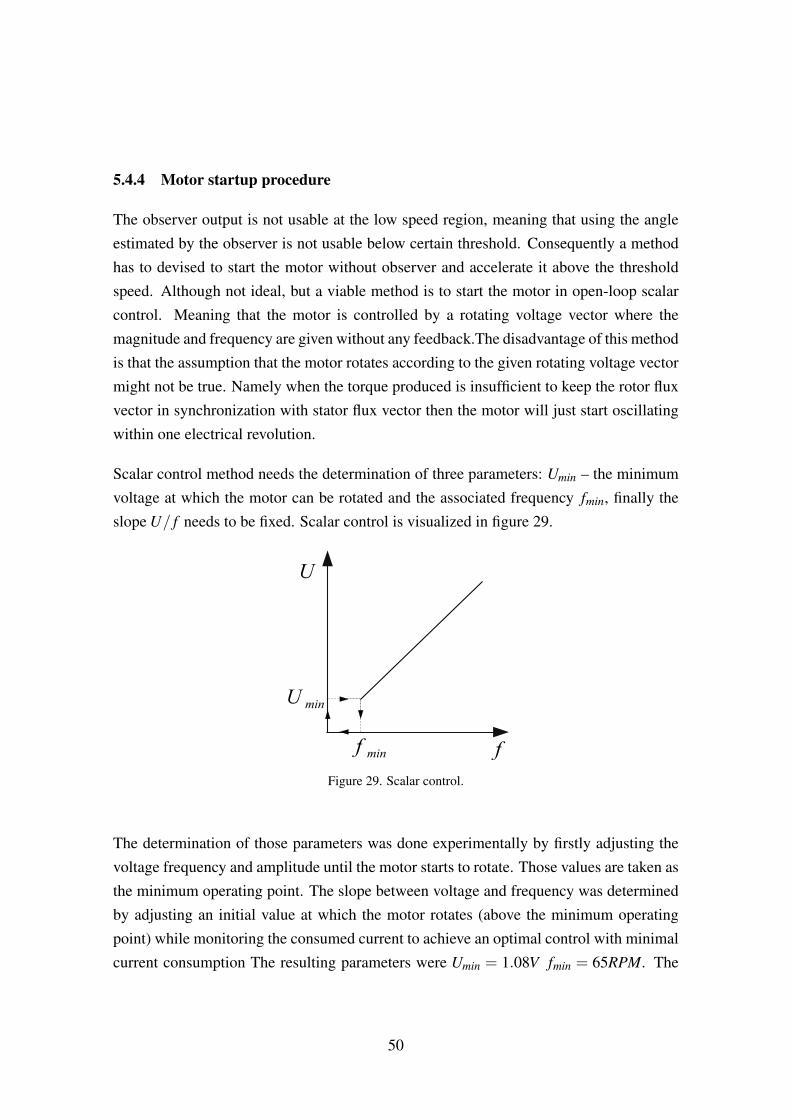
Scalar control method needs the determination of three parameters: Umin – the minimumvoltage at which the motor can be rotated and the associated frequency fmin, finally theslope U/ f needs to be fixed. Scalar control is visualized in figure 29.
Figure 29. Scalar control.
The determination of those parameters was done experimentally by firstly adjusting thevoltage frequency and amplitude until the motor starts to rotate. Those values are taken asthe minimum operating point. The slope between voltage and frequency was determinedby adjusting an initial value at which the motor rotates (above the minimum operatingpoint) while monitoring the consumed current to achieve an optimal control with minimalcurrent consumption The resulting parameters were Umin = 1.08V fmin = 65RPM. The
50
startup routine from zero speed up to target speed ωtrg will consist of two states: scalarcontrol and observer based field oriented control. The transition between them will bedefined by a threshold speed ωthres. When speed of the motor is below ωthres the motoris controlled using scalar control algorithm, when speed passes the threshold control istransferred smoothly to field oriented control. The startup routine is visualized in thefollowing speed-time graph:
Figure 30. Startup graph.
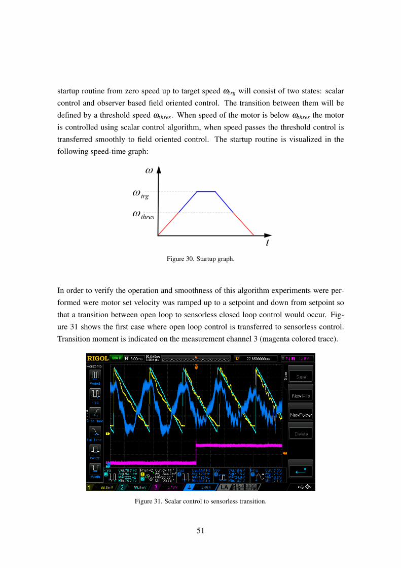
In order to verify the operation and smoothness of this algorithm experiments were per-formed were motor set velocity was ramped up to a setpoint and down from setpoint sothat a transition between open loop to sensorless closed loop control would occur. Fig-ure 31 shows the first case where open loop control is transferred to sensorless control.Transition moment is indicated on the measurement channel 3 (magenta colored trace).
Figure 31. Scalar control to sensorless transition.
51
From the measurements it can be seen that there is no noticeable jump in the motor angle,indicating a smooth transition. Also measurement in channel 4 shows current in one ofthe motor phases. When control is taken over by sensorless observer based algorithm thecurrent drops, as the control is more optimal due to correct angle estimation.
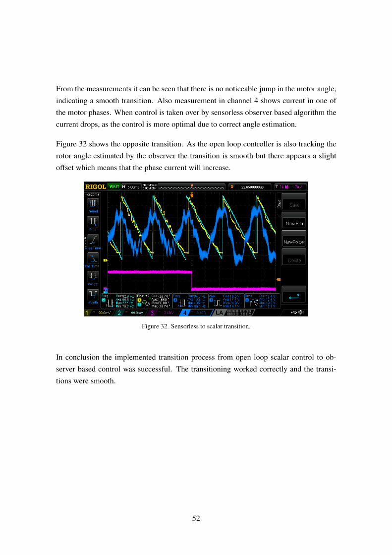
Figure 32 shows the opposite transition. As the open loop controller is also tracking therotor angle estimated by the observer the transition is smooth but there appears a slightoffset which means that the phase current will increase.
Figure 32. Sensorless to scalar transition.
In conclusion the implemented transition process from open loop scalar control to ob-server based control was successful. The transitioning worked correctly and the transi-tions were smooth.
52
5.4.5 Rotational direction reversal
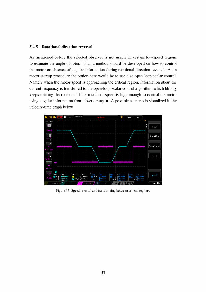
As mentioned before the selected observer is not usable in certain low-speed regionsto estimate the angle of rotor. Thus a method should be developed on how to controlthe motor on absence of angular information during rotational direction reversal. As inmotor startup procedure the option here would be to use also open-loop scalar control.Namely when the motor speed is approaching the critical region, information about thecurrent frequency is transferred to the open-loop scalar control algorithm, which blindlykeeps rotating the motor until the rotational speed is high enough to control the motorusing angular information from observer again. A possible scenario is visualized in thevelocity-time graph below.
Figure 33. Speed reversal and transitioning between critical regions.
53
6 Performance evaluation
This section describes the measurement of the designed controllers performance with re-gards to torque producing current controller step response, angle estimation accuracy,PLL based speed calculation accuracy and the speed controller step response and distur-bance rejection characteristics. All the measurements were made using an oscilloscopeand using the digital to analog converter (DAC) functionality of the microcontroller. Mea-surement results from oscilloscope were stored as a comma separated value (CSV) file andthe plots were made using Matlab, where the measurements were scaled to correct values.
6.1 Quadrature axis current regulator
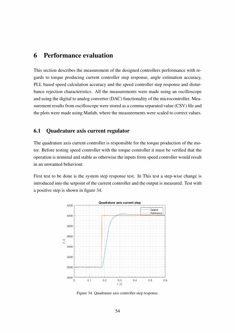
The quadrature axis current controller is responsible for the torque production of the mo-tor. Before testing speed controller with the torque controller it must be verified that theoperation is nominal and stable as otherwise the inputs from speed controller would resultin an unwanted behaviour.
First test to be done is the system step response test. In This test a step-wise change isintroduced into the setpoint of the current controller and the output is measured. Test witha positive step is shown in figure 34.
Figure 34. Quadrature axis controller step response.
54
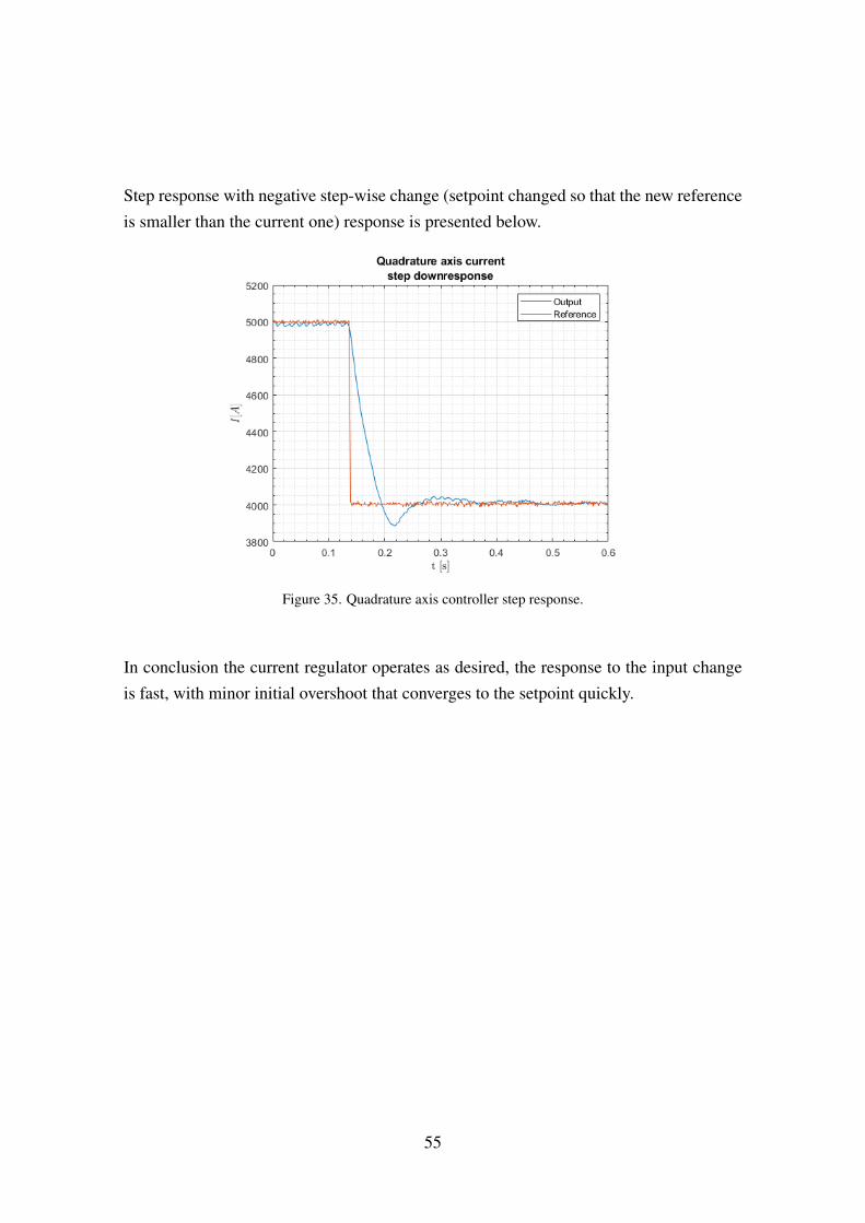
Step response with negative step-wise change (setpoint changed so that the new referenceis smaller than the current one) response is presented below.
Figure 35. Quadrature axis controller step response.
In conclusion the current regulator operates as desired, the response to the input changeis fast, with minor initial overshoot that converges to the setpoint quickly.
55
6.2 Angle estimation accuracy
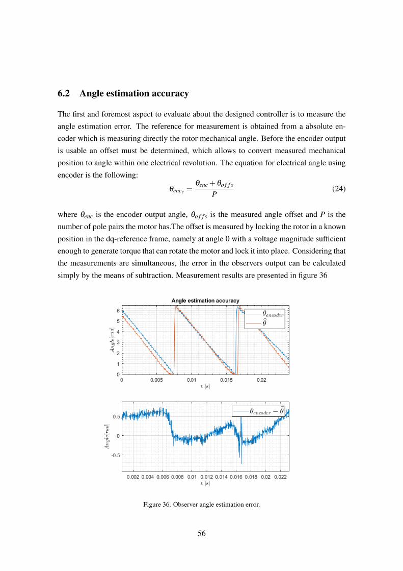
The first and foremost aspect to evaluate about the designed controller is to measure theangle estimation error. The reference for measurement is obtained from a absolute en-coder which is measuring directly the rotor mechanical angle. Before the encoder outputis usable an offset must be determined, which allows to convert measured mechanicalposition to angle within one electrical revolution. The equation for electrical angle usingencoder is the following:
θence =θenc +θo f f s
P(24)
where θenc is the encoder output angle, θo f f s is the measured angle offset and P is thenumber of pole pairs the motor has.The offset is measured by locking the rotor in a knownposition in the dq-reference frame, namely at angle 0 with a voltage magnitude sufficientenough to generate torque that can rotate the motor and lock it into place. Considering thatthe measurements are simultaneous, the error in the observers output can be calculatedsimply by the means of subtraction. Measurement results are presented in figure 36
Figure 36. Observer angle estimation error.
56
From the error calculation it can be seen that the error remains in the range of -0.1 radiansand 0.6 radians, The estimated angle has noticeable ripple, but as can be seen in the fol-lowing experiments didn’t have major effects on speed control quality. In addition duringsome electrical cycles there wasn’t as much absolute error, but there was lag between theactual electrical angle measured by the encoder and the observer estimate.
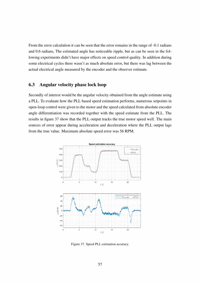
6.3 Angular velocity phase lock loop
Secondly of interest would be the angular velocity obtained from the angle estimate usinga PLL. To evaluate how the PLL based speed estimation performs, numerous setpoints inopen-loop control were given to the motor and the speed calculated from absolute encoderangle differentiation was recorded together with the speed estimate from the PLL. Theresults in figure 37 show that the PLL output tracks the true motor speed well. The mainsources of error appear during acceleration and deceleration where the PLL output lagsfrom the true value. Maximum absolute speed error was 56 RPM.
Figure 37. Speed PLL estimation accuracy.
57
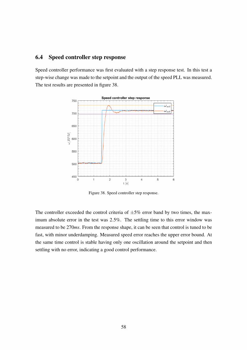
6.4 Speed controller step response
Speed controller performance was first evaluated with a step response test. In this test astep-wise change was made to the setpoint and the output of the speed PLL was measured.The test results are presented in figure 38.
Figure 38. Speed controller step response.
The controller exceeded the control criteria of ±5% error band by two times, the max-imum absolute error in the test was 2.5%. The settling time to this error window wasmeasured to be 270ms. From the response shape, it can be seen that control is tuned to befast, with minor underdamping. Measured speed error reaches the upper error bound. Atthe same time control is stable having only one oscillation around the setpoint and thensettling with no error, indicating a good control performance.
58
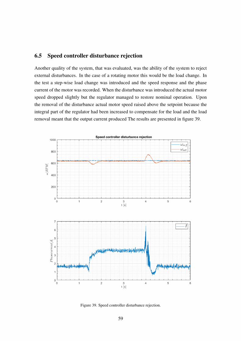
6.5 Speed controller disturbance rejection
Another quality of the system, that was evaluated, was the ability of the system to rejectexternal disturbances. In the case of a rotating motor this would be the load change. Inthe test a step-wise load change was introduced and the speed response and the phasecurrent of the motor was recorded. When the disturbance was introduced the actual motorspeed dropped slightly but the regulator managed to restore nominal operation. Uponthe removal of the disturbance actual motor speed raised above the setpoint because theintegral part of the regulator had been increased to compensate for the load and the loadremoval meant that the output current produced The results are presented in figure 39.
Figure 39. Speed controller disturbance rejection.
59
7 Summary
As a result of this work a brushless DC motor controller hardware with an observer basedsensorless control algorithm was developed. The algorithm was selected from research,investigated and was successfully implemented on a real system, showing that algorithmsdeveloped for permanent magnet synchronous machines can be applicable to small hobby-grade brushless DC motor. In addition methods were developed to measure the electricalparameters of a three phase motors. Phase resistance and inductance measurement wasimplemented using the actual controller and flux linkage measurement using an externalprime mover.
In the beginning of the work problem and end-goal statement was made along with themethods and tools that were going to be used to solve the stated problems. Then a the-oretical overview of three phase motors, their main control principles was made. Thenobserver based control methodology was described and state-of-the-art of observer basedsensorless control of three phase synchronous motors was presented. The required spe-cial hardware for controlling the motor was developed and the main design principles andcomponent choices were presented. During the course of the work this implementationof hardware proved to be reliable and no issues were encountered during implementationof algorithms. Software side of the implementation of the parameter measurements weredone successfully.In addition to implementation of observer based rotor angle estimation,additional control aspects were solved due to the fact that observer based solution was notusable for control at very low speeds.
The final solution that was implemented provides a reference on how sensorless observerbased algorithms could be practically implemented and used with BLDC motors used onmultirotor aerial vehicles. The speed control performance achieved was excellent and canlead the way on using those motors for applications where small-sized, high performancesensorless speed control is required.
60
References[1] Research bulletin: MCUs Sales to Reach Record-High Annual Revenues Through
2022. [Online]. Available: http://www.icinsights.com/data/articles/documents/1101.pdf (visited on 04/29/2018).
[2] J. F. Gieras, Permanent magnet motor technology: design and applications. CRCpress, 2010.
[3] D. C. Hanselman, Brushless permanent magnet motor design. The Writers’ Col-lective, 2003.
[4] K. H. Nam, AC motor control and electrical vehicle applications. CRC press, 2017.[5] F. Giri, AC electric motors control: advanced design techniques and applications.
John Wiley & Sons, 2013.[6] P. Vas, Sensorless vector and direct torque control. Oxford Univ. Press, 1998.[7] K. Ogata and Y. Yang, Modern control engineering. Prentice-Hall, 2002, vol. 4.[8] Q. Tang, A. Shen, X. Luo, and J. Xu, “PMSM sensorless control by injecting HF
pulsating carrier signal into ABC frame”, IEEE Transactions on Power Electronics,vol. 32, no. 5, pp. 3767–3776, 2017.
[9] X. Luo, Q. Tang, A. Shen, and Q. Zhang, “PMSM sensorless control by injectinghf pulsating carrier signal into estimated fixed-frequency rotating reference frame”,IEEE Transactions on Industrial Electronics, vol. 63, no. 4, pp. 2294–2303, 2016.
[10] D. Bao, X. Pan, Y. Wang, X. Wang, and K. Li, “Adaptive synchronous-frequencytracking-mode observer for the sensorless control of a surface pmsm”, IEEE Trans-actions on Industry Applications, vol. 54, no. 6, pp. 6460–6471, 2018.
[11] G. Zhang, G. Wang, D. Xu, and N. Zhao, “ADALINE-network-based pll for posi-tion sensorless interior permanent magnet synchronous motor drives”, IEEE Trans-actions on Power Electronics, vol. 31, no. 2, pp. 1450–1460, 2016.
[12] H. Li, Z. Wang, C. Wen, and X. Wang, “Sensorless Control of Surface-mountedPermanent Magnet Synchronous Motor Drives Using Nonlinear Optimization”,IEEE Transactions on Power Electronics, 2018.
[13] STM32F446ZE High-performance foundation line, ARM Cortex-M4 core withDSP and FPU, 512 Kbytes Flash, 180 MHz CPU, ART Accelerator, Dual QSPI.[Online]. Available: https://www.st.com/content/st_com/en/products/microcontrollers - microprocessors / stm32 - 32 - bit - arm - cortex -mcus / stm32 - high - performance - mcus / stm32f4 - series / stm32f446 /stm32f446ze.html (visited on 04/29/2018).
[14] DRV8305 Three Phase Gate Driver With Current Shunt Amplifiers and VoltageRegulator datasheet (Rev. B). [Online]. Available: http://www.ti.com/lit/ds/symlink/drv8305.pdf (visited on 04/29/2018).
[15] Nanotec motor image. [Online]. Available: https : / / en . nanotec . com /fileadmin/_processed_/8/5/csm_DF45M_A2_2fc381809f.jpg (visitedon 04/29/2018).
[16] Nanotec motor datasheet. [Online]. Available: https : / / en . nanotec . com /fileadmin/files/Datenblaetter/BLDC/DF45/DF45L024048-A2.pdf (vis-ited on 04/29/2018).
[17] NTM PROPDRIVE v2 3536 910KV Brushless Outrunner Motor. [Online]. Avail-able: https : / / hobbyking . com / en _ us / propdrive - v2 - 3536a - 910kv -brushless-outrunner-motor.html (visited on 04/29/2018).
61

[18] R. Ortega, L. Praly, A. Astolfi, J. Lee, and K. Nam, “Estimation of rotor positionand speed of permanent magnet synchronous motors with guaranteed stability”,IEEE Transactions on Control Systems Technology, vol. 19, no. 3, pp. 601–614,2011.
[19] J. Lee, J. Hong, K. Nam, R. Ortega, L. Praly, and A. Astolfi, “Sensorless con-trol of surface-mount permanent-magnet synchronous motors based on a nonlinearobserver”, IEEE Transactions on power electronics, vol. 25, no. 2, pp. 290–297,2010.
62
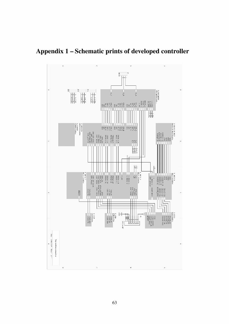
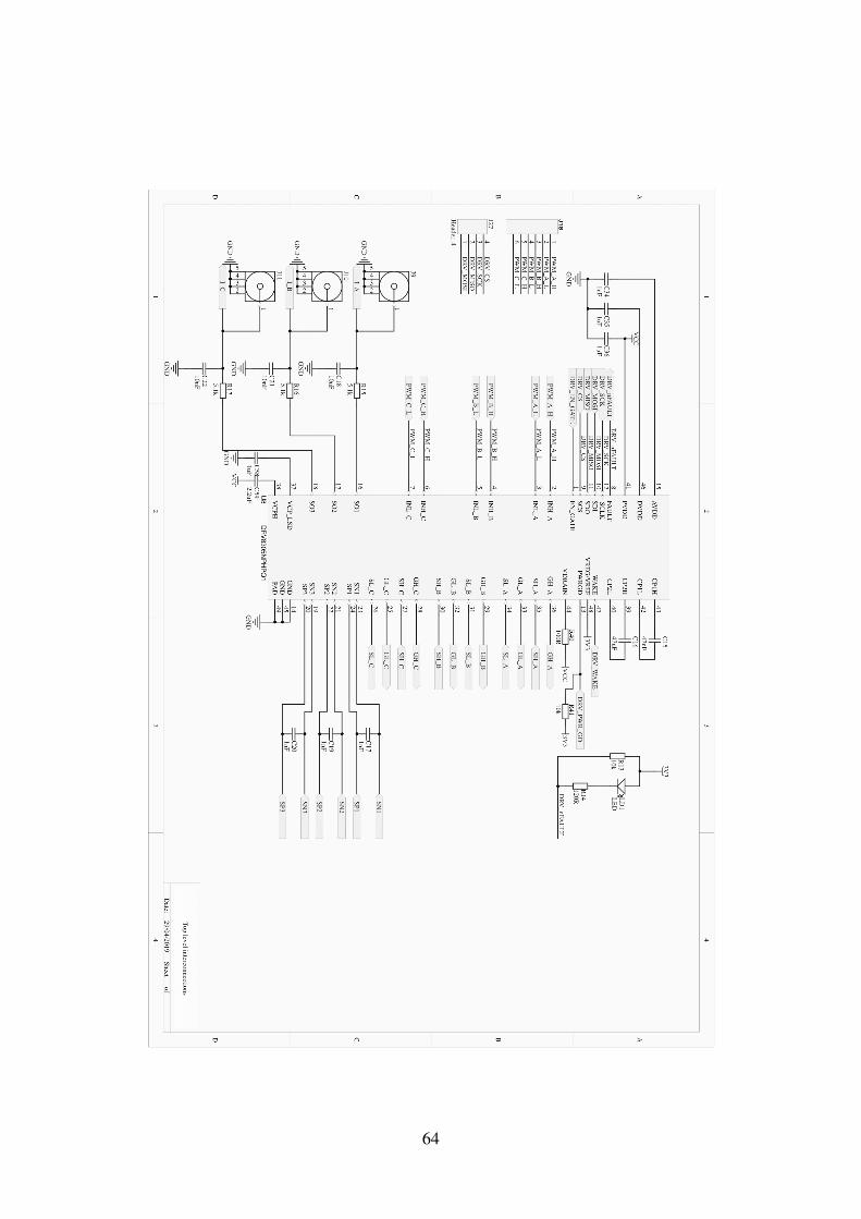
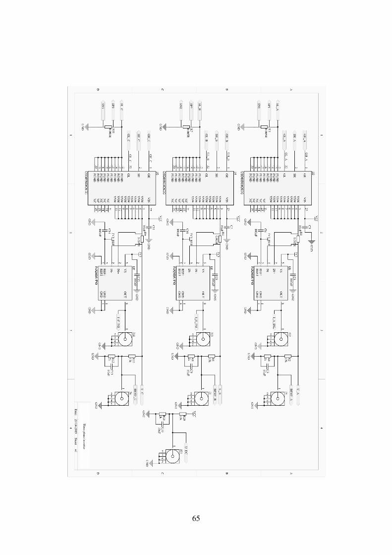
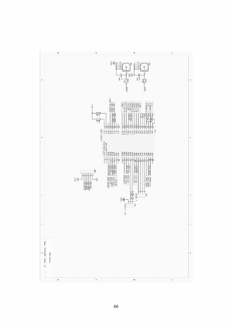
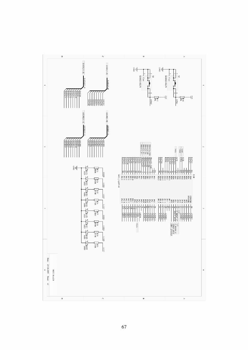
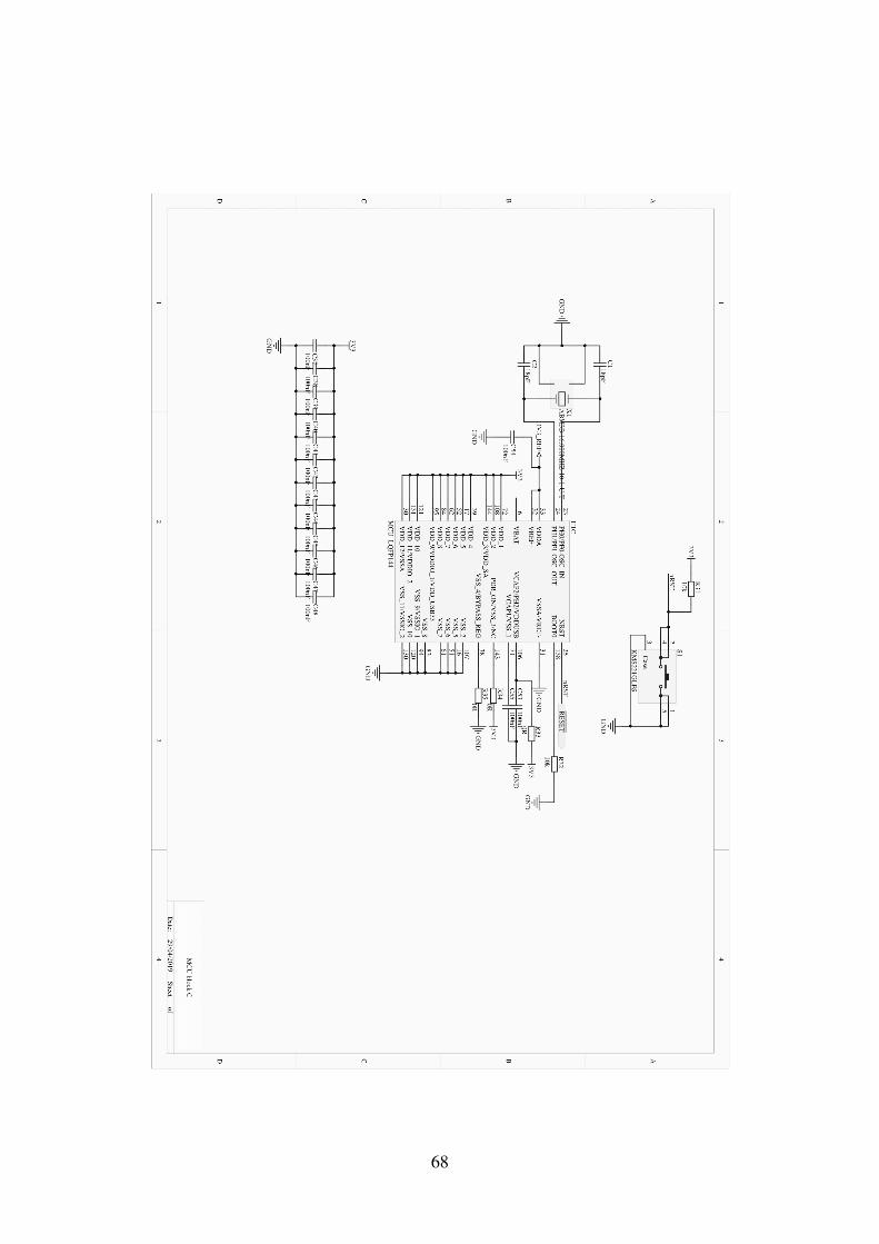
Appendix 1 – Schematic prints of developed controller
63
64
65
66
67
68

69
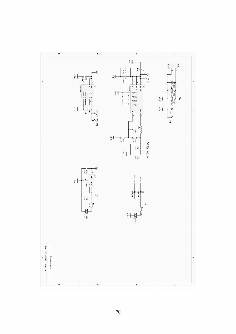
70
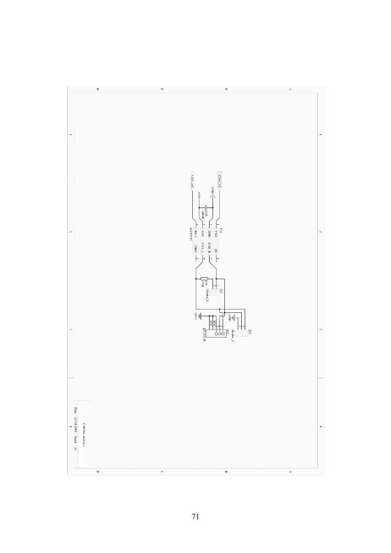
71
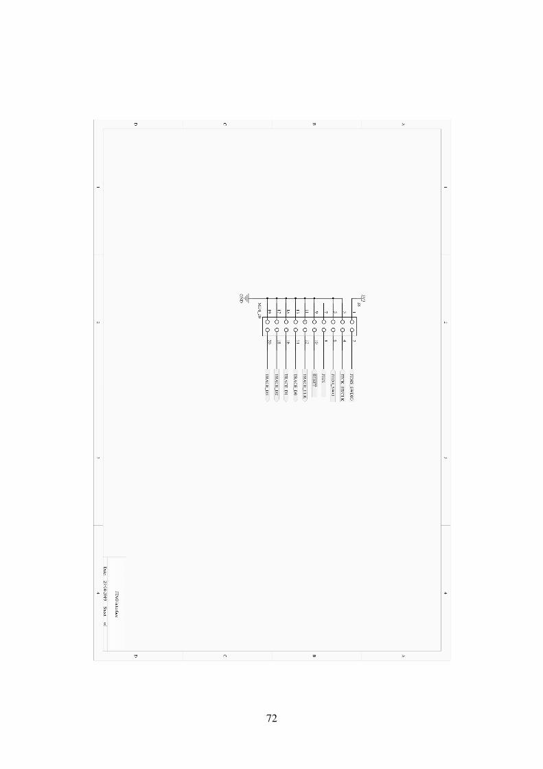
72
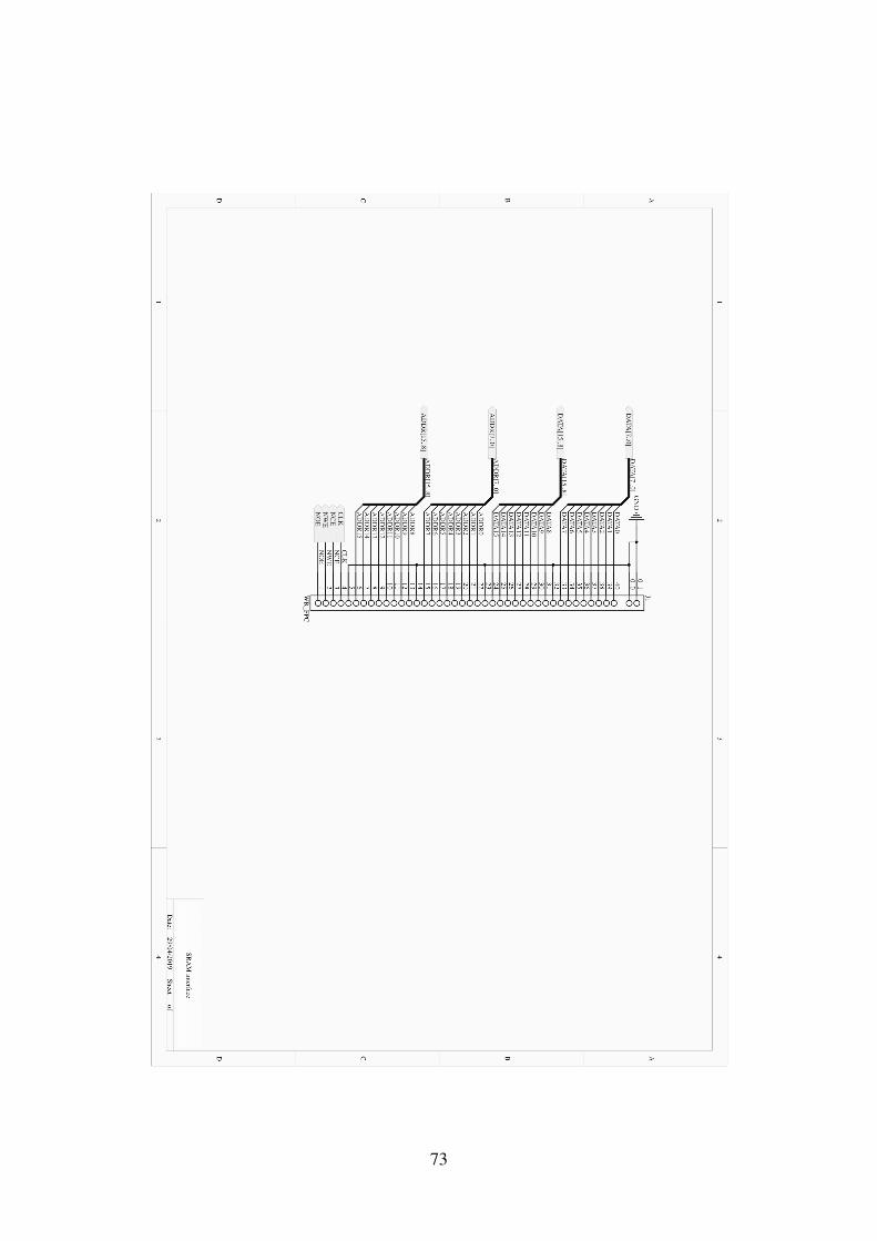
73
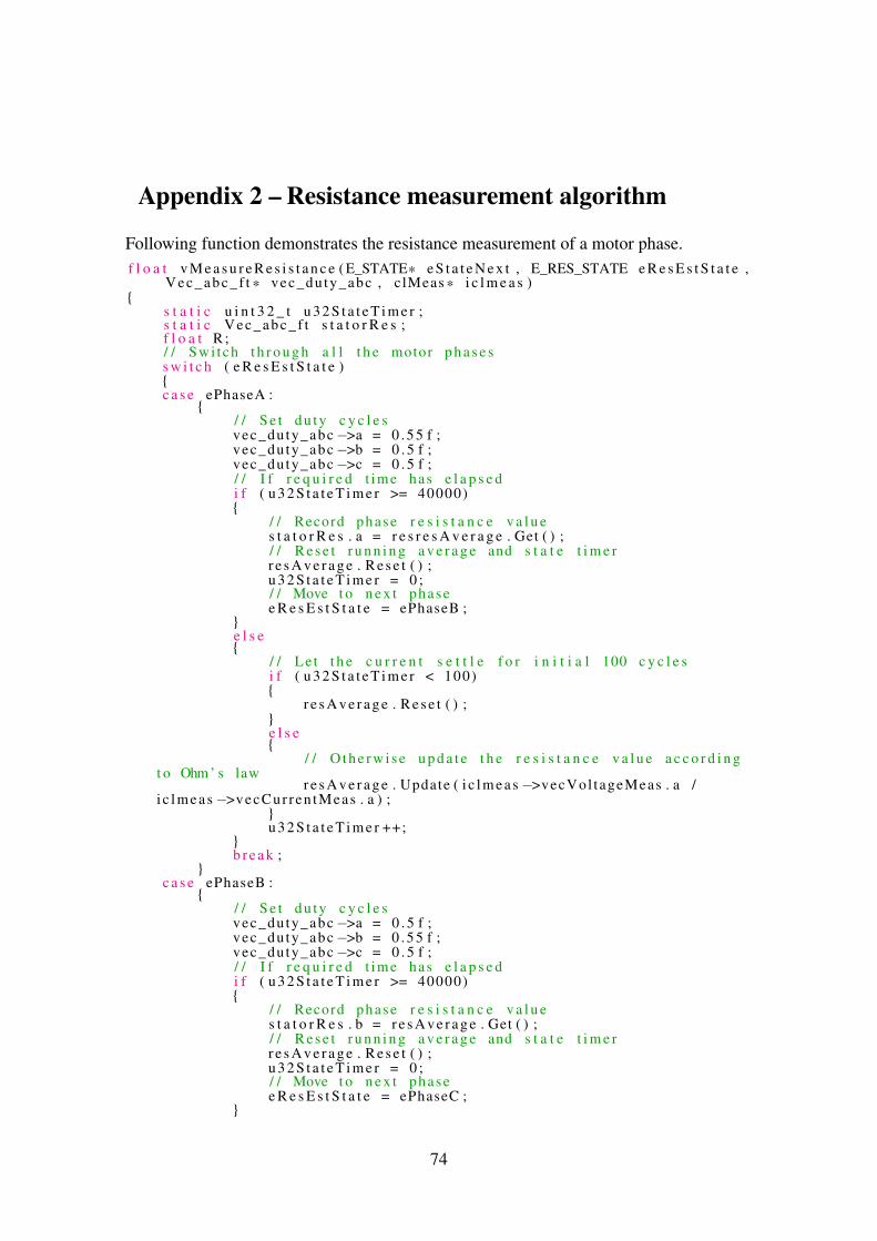
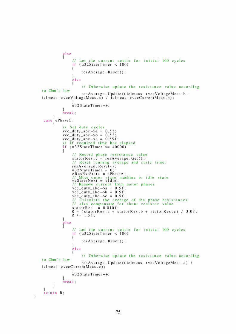
Appendix 2 – Resistance measurement algorithm
Following function demonstrates the resistance measurement of a motor phase.f l o a t v M e a s u r e R e s i s t a n c e ( E_STATE* e S t a t e N e x t , E_RES_STATE e R e s E s t S t a t e ,
V e c _ a b c _ f t * vec_du ty_abc , c lMeas * i c l m e a s )
s t a t i c u i n t 3 2 _ t u 3 2 S t a t e T i m e r ;s t a t i c V e c _ a b c _ f t s t a t o r R e s ;f l o a t R ;/ / Swi tch t h r o u g h a l l t h e motor p h a s e ss w i t c h ( e R e s E s t S t a t e )c a s e ePhaseA :
/ / S e t du ty c y c l e svec_du ty_abc−>a = 0 . 5 5 f ;vec_du ty_abc−>b = 0 . 5 f ;vec_du ty_abc−>c = 0 . 5 f ;/ / I f r e q u i r e d t ime has e l a p s e di f ( u 3 2 S t a t e T i m e r >= 40000)
/ / Record phase r e s i s t a n c e v a l u es t a t o r R e s . a = r e s r e s A v e r a g e . Get ( ) ;/ / R e s e t r u n n i n g a v e r a g e and s t a t e t i m e rr e s A v e r a g e . R e s e t ( ) ;u 3 2 S t a t e T i m e r = 0 ;/ / Move t o n e x t phasee R e s E s t S t a t e = ePhaseB ;
e l s e
/ / Le t t h e c u r r e n t s e t t l e f o r i n i t i a l 100 c y c l e si f ( u 3 2 S t a t e T i m e r < 100)
r e s A v e r a g e . R e s e t ( ) ;e l s e
/ / O t h e r w i s e u p d a t e t h e r e s i s t a n c e v a l u e a c c o r d i n gt o Ohm ’ s law
r e s A v e r a g e . Update ( i c l m e a s−>vecVol tageMeas . a /i c l m e a s−>vecCur ren tMeas . a ) ;
u 3 2 S t a t e T i m e r ++;
b r e a k ;
c a s e ePhaseB :
/ / S e t du ty c y c l e svec_du ty_abc−>a = 0 . 5 f ;vec_du ty_abc−>b = 0 . 5 5 f ;vec_du ty_abc−>c = 0 . 5 f ;/ / I f r e q u i r e d t ime has e l a p s e di f ( u 3 2 S t a t e T i m e r >= 40000)
/ / Record phase r e s i s t a n c e v a l u es t a t o r R e s . b = r e s A v e r a g e . Get ( ) ;/ / R e s e t r u n n i n g a v e r a g e and s t a t e t i m e rr e s A v e r a g e . R e s e t ( ) ;u 3 2 S t a t e T i m e r = 0 ;/ / Move t o n e x t phasee R e s E s t S t a t e = ePhaseC ;
74
e l s e
/ / Le t t h e c u r r e n t s e t t l e f o r i n i t i a l 100 c y c l e si f ( u 3 2 S t a t e T i m e r < 100)
r e s A v e r a g e . R e s e t ( ) ;e l s e
/ / O t h e r w i s e u p d a t e t h e r e s i s t a n c e v a l u e a c c o r d i n gt o Ohm ’ s law
r e s A v e r a g e . Update ( ( i c l m e a s−>vecVol tageMeas . b −i c l m e a s−>vecVol tageMeas . a ) / i c l m e a s−>vecCur ren tMeas . b ) ;
u 3 2 S t a t e T i m e r ++;
b r e a k ;
c a s e ePhaseC :
/ / S e t du ty c y c l e svec_du ty_abc−>a = 0 . 5 f ;vec_du ty_abc−>b = 0 . 5 f ;vec_du ty_abc−>c = 0 . 5 5 f ;/ / I f r e q u i r e d t ime has e l a p s e di f ( u 3 2 S t a t e T i m e r >= 40000)
/ / Record phase r e s i s t a n c e v a l u es t a t o r R e s . c = r e s A v e r a g e . Get ( ) ;/ / R e s e t r u n n i n g a v e r a g e and s t a t e t i m e rr e s A v e r a g e . R e s e t ( ) ;u 3 2 S t a t e T i m e r = 0 ;e R e s E s t S t a t e = ePhaseA ;/ / Move o u t e r s t a t e machine t o i d l e s t a t e* e S t a t e N e x t = e I d l e ;/ / Remove c u r r e n t from motor p h a s e svec_du ty_abc−>a = 0 . 5 f ;vec_du ty_abc−>b = 0 . 5 f ;vec_du ty_abc−>c = 0 . 5 f ;/ / C a l c u l a t e t h e a v e r a g e o f t h e phase r e s i s t a n c e s/ / a l s o compensa te f o r s h u n t r e s i s t o r v a l u es t a t o r R e s −= 0 .010 f ;R = ( s t a t o r R e s . a + s t a t o r R e s . b + s t a t o r R e s . c ) / 3 . 0 f ;R /= 1 . 5 f ;
e l s e
/ / Le t t h e c u r r e n t s e t t l e f o r i n i t i a l 100 c y c l e si f ( u 3 2 S t a t e T i m e r < 100)
r e s A v e r a g e . R e s e t ( ) ;e l s e
/ / O t h e r w i s e u p d a t e t h e r e s i s t a n c e v a l u e a c c o r d i n gt o Ohm ’ s law
r e s A v e r a g e . Update ( ( i c l m e a s−>vecVol tageMeas . c ) /i c l m e a s−>vecCur ren tMeas . c ) ;
u 3 2 S t a t e T i m e r ++;
b r e a k ;
r e t u r n R ;
75
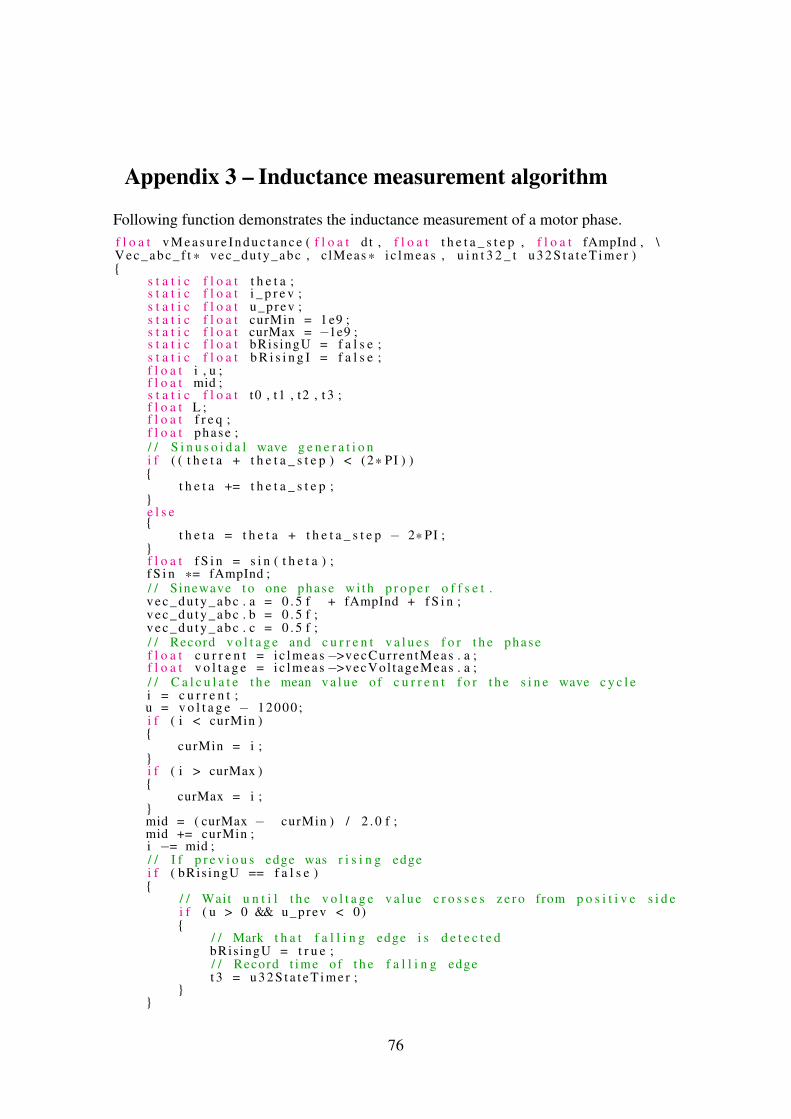
Appendix 3 – Inductance measurement algorithm
Following function demonstrates the inductance measurement of a motor phase.f l o a t v M e a s u r e I n d u c t a n c e ( f l o a t d t , f l o a t t h e t a _ s t e p , f l o a t fAmpInd , \V e c _ a b c _ f t * vec_du ty_abc , c lMeas * i c l m e a s , u i n t 3 2 _ t u 3 2 S t a t e T i m e r )
s t a t i c f l o a t t h e t a ;s t a t i c f l o a t i _ p r e v ;s t a t i c f l o a t u_prev ;s t a t i c f l o a t curMin = 1 e9 ;s t a t i c f l o a t curMax = −1e9 ;s t a t i c f l o a t bRis ingU = f a l s e ;s t a t i c f l o a t b R i s i n g I = f a l s e ;f l o a t i , u ;f l o a t mid ;s t a t i c f l o a t t0 , t1 , t2 , t 3 ;f l o a t L ;f l o a t f r e q ;f l o a t phase ;/ / S i n u s o i d a l wave g e n e r a t i o ni f ( ( t h e t a + t h e t a _ s t e p ) < (2* PI ) )
t h e t a += t h e t a _ s t e p ;e l s e
t h e t a = t h e t a + t h e t a _ s t e p − 2* PI ;f l o a t f S i n = s i n ( t h e t a ) ;f S i n *= fAmpInd ;/ / Sinewave t o one phase wi th p r o p e r o f f s e t .v e c _ d u t y _ a b c . a = 0 . 5 f + fAmpInd + f S i n ;v e c _ d u t y _ a b c . b = 0 . 5 f ;v e c _ d u t y _ a b c . c = 0 . 5 f ;/ / Record v o l t a g e and c u r r e n t v a l u e s f o r t h e phasef l o a t c u r r e n t = i c l m e a s−>vecCur ren tMeas . a ;f l o a t v o l t a g e = i c l m e a s−>vecVol tageMeas . a ;/ / C a l c u l a t e t h e mean v a l u e o f c u r r e n t f o r t h e s i n e wave c y c l ei = c u r r e n t ;u = v o l t a g e − 12000 ;i f ( i < curMin )
curMin = i ;i f ( i > curMax )
curMax = i ;mid = ( curMax − curMin ) / 2 . 0 f ;mid += curMin ;i −= mid ;/ / I f p r e v i o u s edge was r i s i n g edgei f ( bRis ingU == f a l s e )
/ / Wait u n t i l t h e v o l t a g e v a l u e c r o s s e s z e r o from p o s i t i v e s i d ei f ( u > 0 && u_prev < 0)
/ / Mark t h a t f a l l i n g edge i s d e t e c t e dbRis ingU = t r u e ;/ / Record t ime of t h e f a l l i n g edget 3 = u 3 2 S t a t e T i m e r ;
76
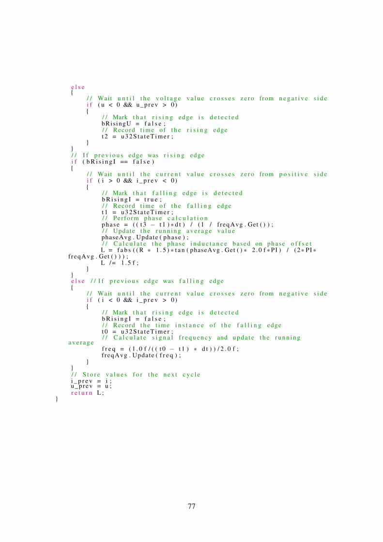
e l s e
/ / Wait u n t i l t h e v o l t a g e v a l u e c r o s s e s z e r o from n e g a t i v e s i d ei f ( u < 0 && u_prev > 0)
/ / Mark t h a t r i s i n g edge i s d e t e c t e dbRis ingU = f a l s e ;/ / Record t ime of t h e r i s i n g edget 2 = u 3 2 S t a t e T i m e r ;
/ / I f p r e v i o u s edge was r i s i n g edgei f ( b R i s i n g I == f a l s e )
/ / Wait u n t i l t h e c u r r e n t v a l u e c r o s s e s z e r o from p o s i t i v e s i d ei f ( i > 0 && i _ p r e v < 0)
/ / Mark t h a t f a l l i n g edge i s d e t e c t e db R i s i n g I = t r u e ;/ / Record t ime of t h e f a l l i n g edget 1 = u 3 2 S t a t e T i m e r ;/ / Per fo rm phase c a l c u l a t i o nphase = ( ( t 3 − t 1 ) * d t ) / (1 / f reqAvg . Get ( ) ) ;/ / Update t h e r u n n i n g a v e r a g e v a l u ephaseAvg . Update ( phase ) ;/ / C a l c u l a t e t h e phase i n d u c t a n c e based on phase o f f s e tL = f a b s ( ( R * 1 . 5 ) * t a n ( phaseAvg . Get ( ) * 2 . 0 f * PI ) / (2* PI *
freqAvg . Get ( ) ) ) ;L /= 1 . 5 f ;
e l s e / / I f p r e v i o u s edge was f a l l i n g edge
/ / Wait u n t i l t h e c u r r e n t v a l u e c r o s s e s z e r o from n e g a t i v e s i d ei f ( i < 0 && i _ p r e v > 0)
/ / Mark t h a t r i s i n g edge i s d e t e c t e db R i s i n g I = f a l s e ;/ / Record t h e t ime i n s t a n c e o f t h e f a l l i n g edget 0 = u 3 2 S t a t e T i m e r ;/ / C a l c u l a t e s i g n a l f r e q u e n c y and u p d a t e t h e r u n n i n g
a v e r a g ef r e q = ( 1 . 0 f / ( ( t 0 − t 1 ) * d t ) ) / 2 . 0 f ;f reqAvg . Update ( f r e q ) ;
/ / S t o r e v a l u e s f o r t h e n e x t c y c l ei _ p r e v = i ;u_prev = u ;r e t u r n L ;
77

Appendix 4 – Source code
Complete program source code implemented on the microcontroller is attached as a CDto this work.
78