© Eric Xing @ CMU, 2006-2009 1

Machine Learning

Computational Learning Theory

Eric Xing

Lecture 5, August 13, 2010

Reading:

© Eric Xing @ CMU, 2006-2009 2

Generalizability of Learning In machine learning it's really the generalization error that we

care about, but most learning algorithms fit their models to the training set.

Why should doing well on the training set tell us anything about generalization error? Specifically, can we relate error on to training set to generalization error?

Are there conditions under which we can actually prove that learning algorithms will work well?

© Eric Xing @ CMU, 2006-2009 3

What General Lawsconstrain Inductive Learning?

Sample Complexity How many training examples are sufficient

to learn target concept?

Computational Complexity Resources required to learn target concept?

Want theory to relate: Training examples

Quantity Quality m How presented

Complexity of hypothesis/concept space H Accuracy of approx to target concept ε Probability of successful learning δ

© Eric Xing @ CMU, 2006-2009 4

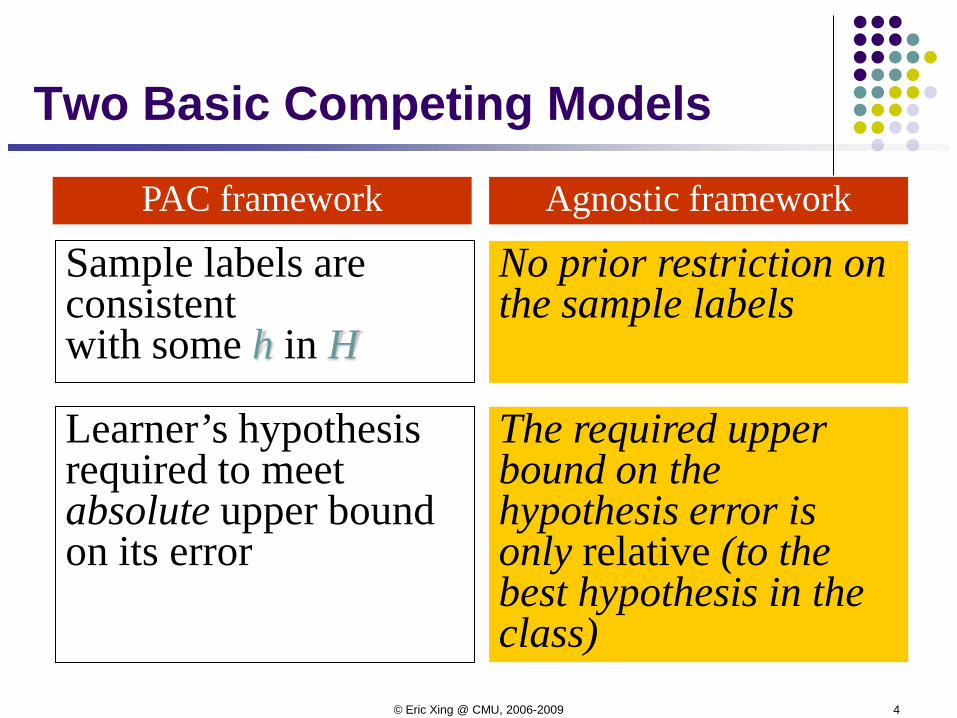
Sample labels are consistentwith some h in H

Learner’s hypothesis required to meet absolute upper boundon its error

No prior restriction on the sample labels

The required upper bound on the hypothesis error is only relative (to the best hypothesis in the class)

PAC framework Agnostic framework

Two Basic Competing Models

© Eric Xing @ CMU, 2006-2009 5

ProtocolLearner

N

N

Y

So

…

…

…

…

NoPale8710

::::

YesClear11022

NoPale9535

diseaseX

Colour

Press.

Temp

.

ClassifierPale

…N90

32

Color

…

Sore-Throat

Press.

Temp

No

diseaseX

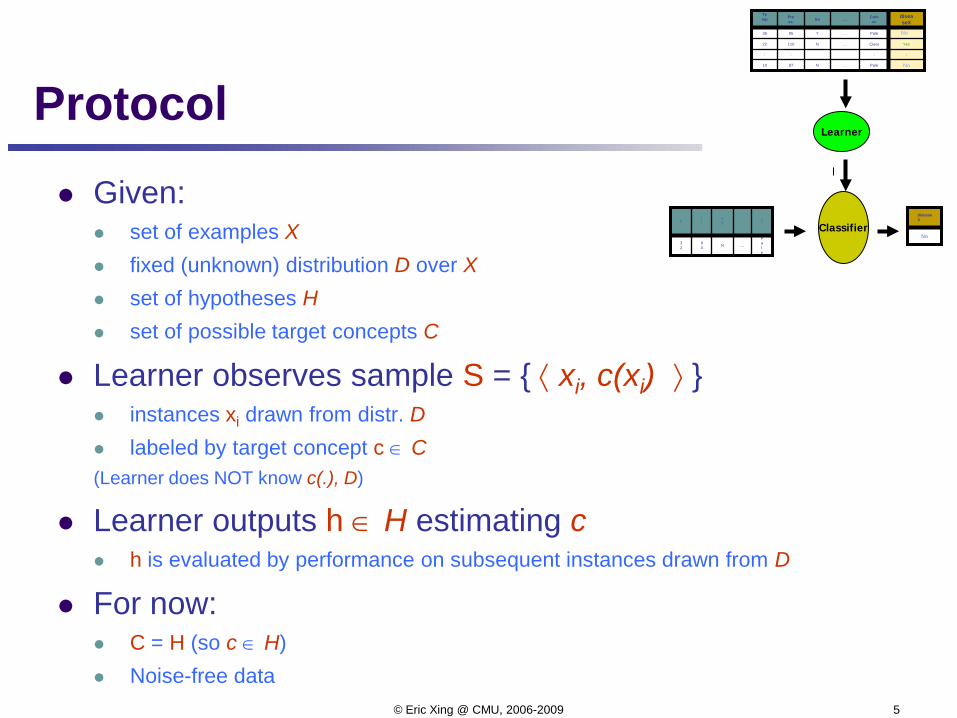
Given: set of examples X fixed (unknown) distribution D over X set of hypotheses H set of possible target concepts C

Learner observes sample S = { ⟨ xi, c(xi) ⟩ } instances xi drawn from distr. D labeled by target concept c ∈ C(Learner does NOT know c(.), D)

Learner outputs h ∈ H estimating c h is evaluated by performance on subsequent instances drawn from D

For now: C = H (so c ∈ H) Noise-free data

© Eric Xing @ CMU, 2006-2009 6

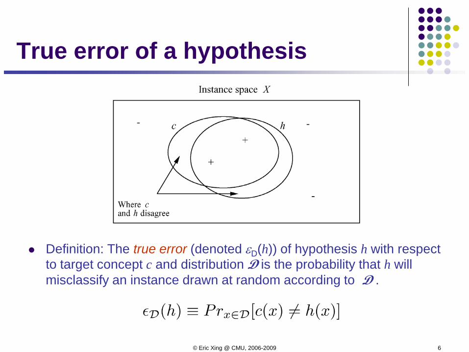
True error of a hypothesis

Definition: The true error (denoted εD(h)) of hypothesis h with respect to target concept c and distribution D is the probability that h will misclassify an instance drawn at random according to D .

© Eric Xing @ CMU, 2006-2009 7

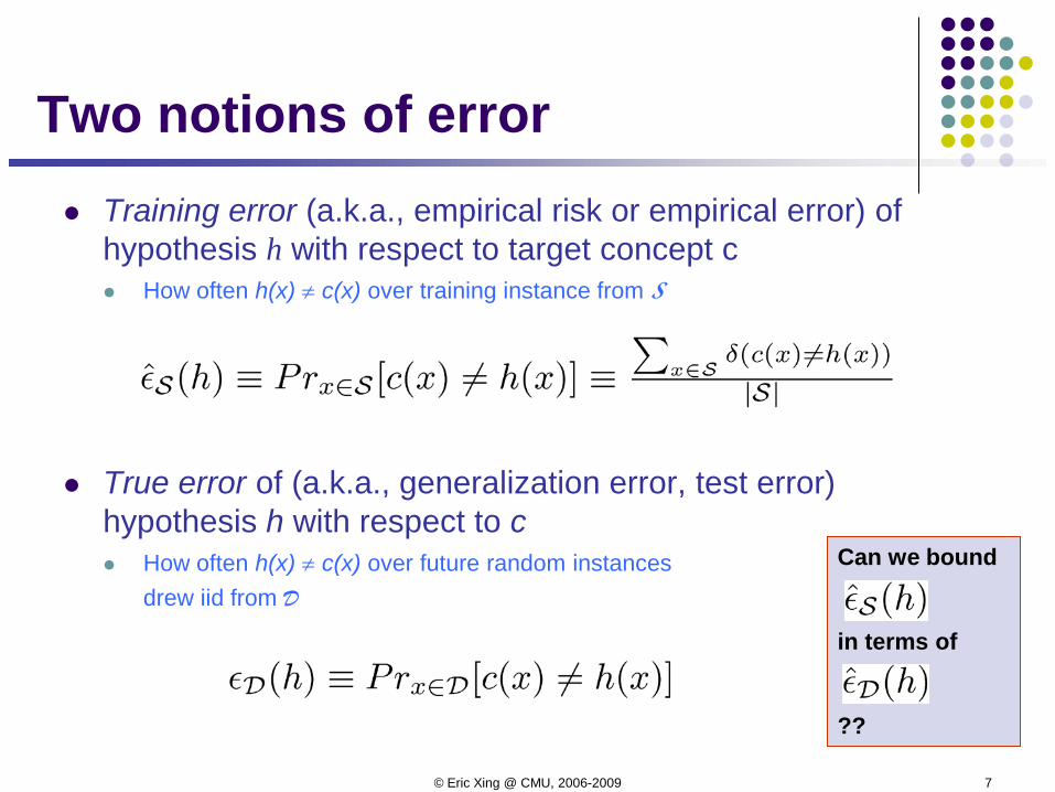
Two notions of error Training error (a.k.a., empirical risk or empirical error) of

hypothesis h with respect to target concept c How often h(x) ≠ c(x) over training instance from S

True error of (a.k.a., generalization error, test error) hypothesis h with respect to c How often h(x) ≠ c(x) over future random instances

drew iid from D

Can we bound

in terms of

??

© Eric Xing @ CMU, 2006-2009 8

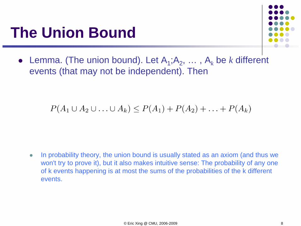
The Union Bound Lemma. (The union bound). Let A1;A2, … , Ak be k different

events (that may not be independent). Then

In probability theory, the union bound is usually stated as an axiom (and thus we won't try to prove it), but it also makes intuitive sense: The probability of any one of k events happening is at most the sums of the probabilities of the k different events.

© Eric Xing @ CMU, 2006-2009 9

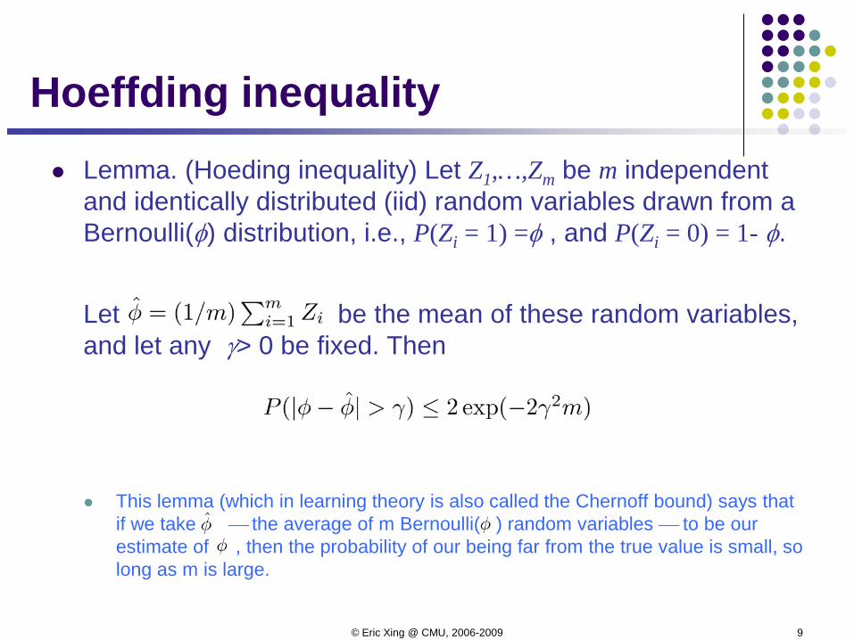
Hoeffding inequality Lemma. (Hoeding inequality) Let Z1,…,Zm be m independent

and identically distributed (iid) random variables drawn from a Bernoulli(φ) distribution, i.e., P(Zi = 1) =φ , and P(Zi = 0) = 1- φ.

Let be the mean of these random variables, and let any γ> 0 be fixed. Then

This lemma (which in learning theory is also called the Chernoff bound) says that if we take the average of m Bernoulli( ) random variables to be our estimate of , then the probability of our being far from the true value is small, so long as m is large.

© Eric Xing @ CMU, 2006-2009 10

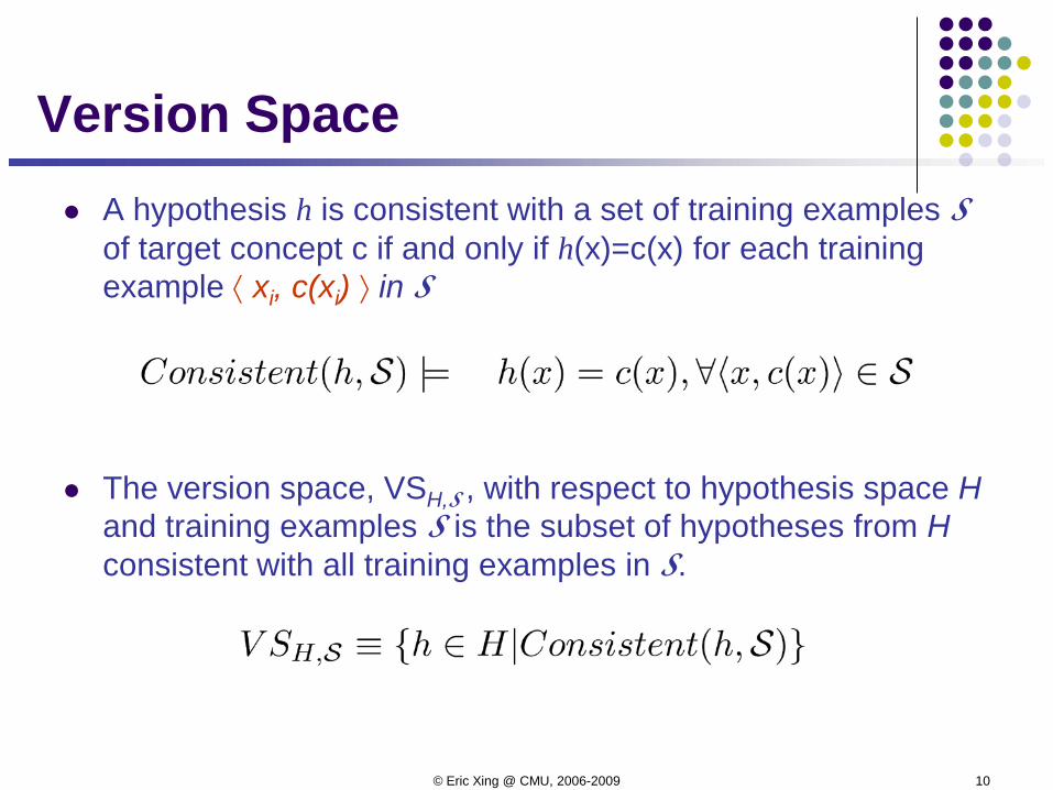
Version Space A hypothesis h is consistent with a set of training examples S

of target concept c if and only if h(x)=c(x) for each training example ⟨ xi, c(xi) ⟩ in S

The version space, VSH,S , with respect to hypothesis space Hand training examples S is the subset of hypotheses from Hconsistent with all training examples in S.

© Eric Xing @ CMU, 2006-2009 11

Consistent Learner A learner is consistent if it outputs hypothesis that perfectly

fits the training data This is a quite reasonable learning strategy

Every consistent learning outputs a hypothesis belonging to the version space

We want to know how such hypothesis generalizes

© Eric Xing @ CMU, 2006-2009 12

Probably Approximately Correct

Goal:PAC-Learner produces hypothesis ĥ that

is approximately correct,errD(ĥ) ≈ 0

with high probability

P( errD(ĥ) ≈ 0 ) ≈ 1

Double “hedging" approximately probably

Need both!

© Eric Xing @ CMU, 2006-2009 13

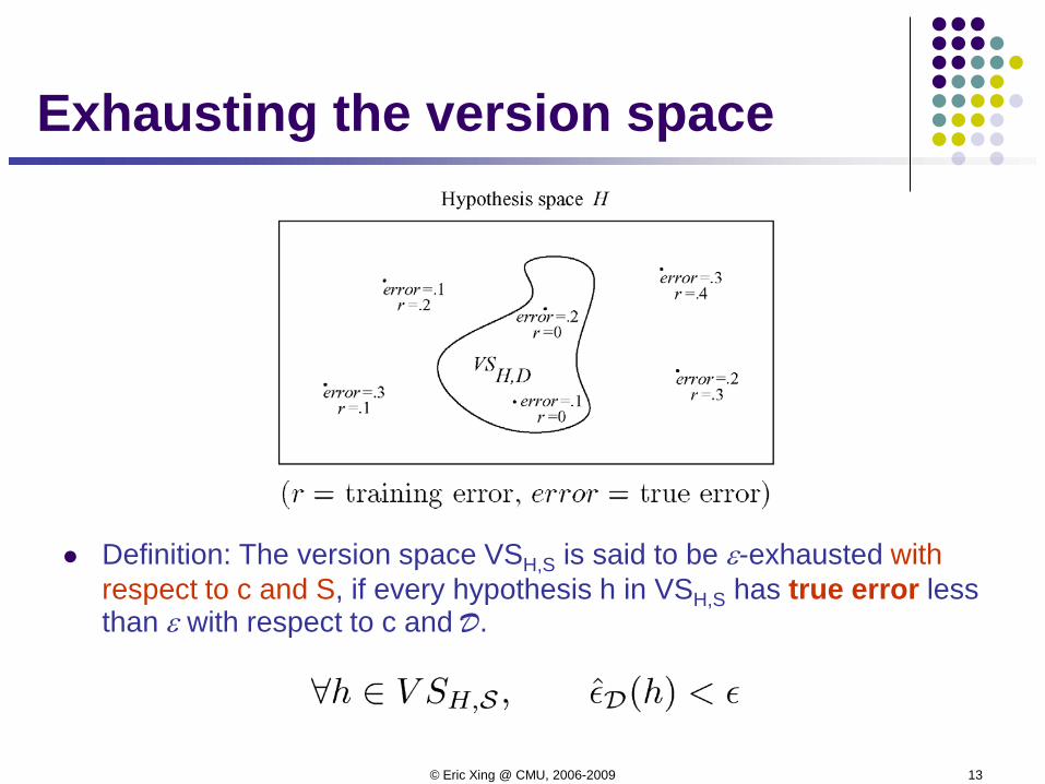
Definition: The version space VSH,S is said to be ε-exhausted with respect to c and S, if every hypothesis h in VSH,S has true error less than ε with respect to c and D.

Exhausting the version space

© Eric Xing @ CMU, 2006-2009 14

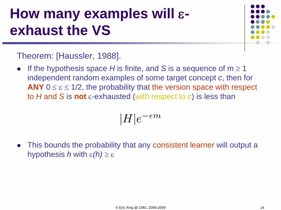
How many examples will ε-exhaust the VS

Theorem: [Haussler, 1988]. If the hypothesis space H is finite, and S is a sequence of m ≥ 1

independent random examples of some target concept c, then for ANY 0 ≤ ε ≤ 1/2, the probability that the version space with respect to H and S is not ε-exhausted (with respect to c) is less than

This bounds the probability that any consistent learner will output a hypothesis h with ε(h) ≥ ε

© Eric Xing @ CMU, 2006-2009 15

Proof

© Eric Xing @ CMU, 2006-2009 16

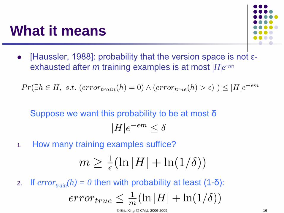
What it means [Haussler, 1988]: probability that the version space is not ε-

exhausted after m training examples is at most |H|e-εm

Suppose we want this probability to be at most δ

1. How many training examples suffice?

2. If errortrain(h) = 0 then with probability at least (1-δ):

© Eric Xing @ CMU, 2006-2009 17

PAC LearnabilityA learning algorithm is PAC learnable if it

Requires no more than polynomial computation per training example, and

no more than polynomial number of samples

Theorem: conjunctions of Boolean literals is PAC learnable

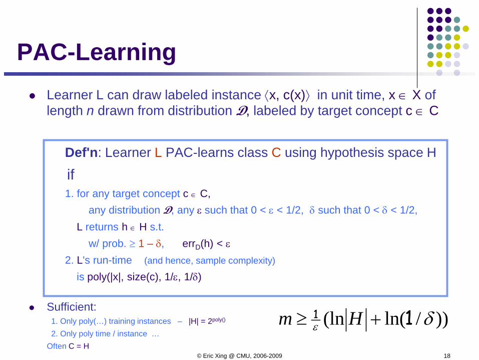
© Eric Xing @ CMU, 2006-2009 18

Learner L can draw labeled instance ⟨x, c(x)⟩ in unit time, x ∈ X of length n drawn from distribution D, labeled by target concept c ∈ C

Def'n: Learner L PAC-learns class C using hypothesis space H

if1. for any target concept c ∈ C,

any distribution D, any ε such that 0 < ε < 1/2, δ such that 0 < δ < 1/2,L returns h ∈ H s.t.

w/ prob. ≥ 1 – δ, errD(h) < ε2. L's run-time (and hence, sample complexity)

is poly(|x|, size(c), 1/ε, 1/δ)

Sufficient:1. Only poly(…) training instances – |H| = 2poly()

2. Only poly time / instance …Often C = H

PAC-Learning

))/ln((ln δε 11 +≥ Hm

© Eric Xing @ CMU, 2006-2009 19

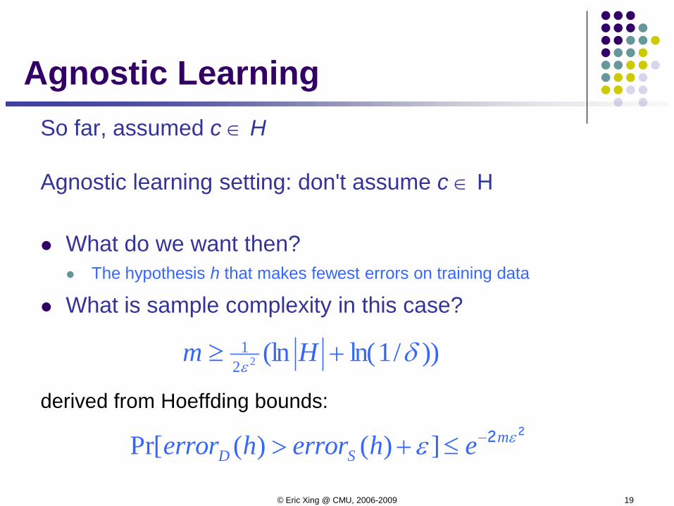
So far, assumed c ∈ H

Agnostic learning setting: don't assume c ∈ H

What do we want then? The hypothesis h that makes fewest errors on training data

What is sample complexity in this case?

derived from Hoeffding bounds:

))/1ln((ln221 δε

+≥ Hm

22 εε mSD eherrorherror −≤+> ])()(Pr[

Agnostic Learning

© Eric Xing @ CMU, 2006-2009 20

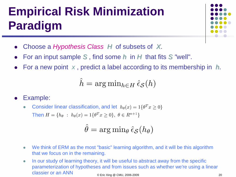
Empirical Risk Minimization Paradigm Choose a Hypothesis Class H of subsets of X. For an input sample S , find some h in H that fits S "well". For a new point x , predict a label according to its membership in h.

Example: Consider linear classification, and let

Then

We think of ERM as the most "basic" learning algorithm, and it will be this algorithm that we focus on in the remaining.

In our study of learning theory, it will be useful to abstract away from the specific parameterization of hypotheses and from issues such as whether we're using a linear classier or an ANN

© Eric Xing @ CMU, 2006-2009 21

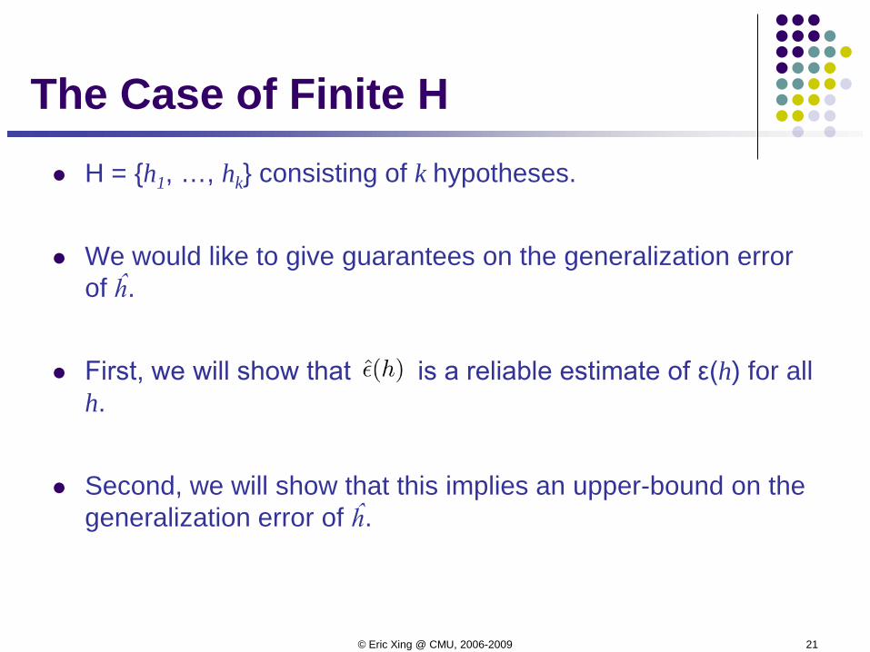
The Case of Finite H H = {h1, …, hk} consisting of k hypotheses.

We would like to give guarantees on the generalization error of ĥ.

First, we will show that is a reliable estimate of ε(h) for all h.

Second, we will show that this implies an upper-bound on the generalization error of ĥ.

© Eric Xing @ CMU, 2006-2009 22

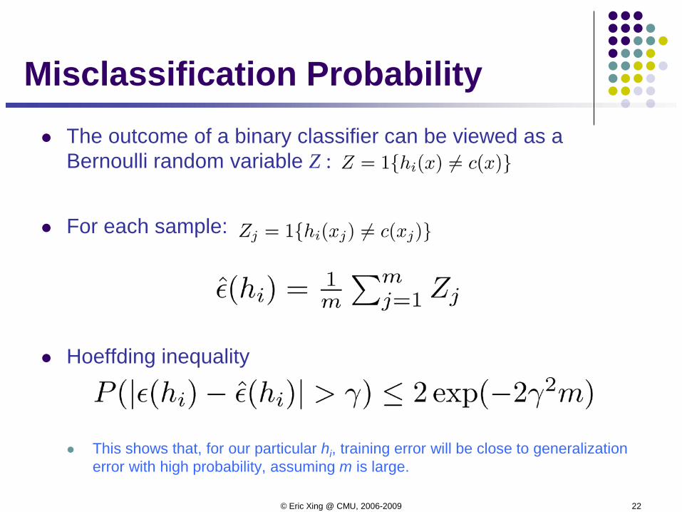
Misclassification Probability The outcome of a binary classifier can be viewed as a

Bernoulli random variable Z :

For each sample:

Hoeffding inequality

This shows that, for our particular hi, training error will be close to generalization error with high probability, assuming m is large.

© Eric Xing @ CMU, 2006-2009 23

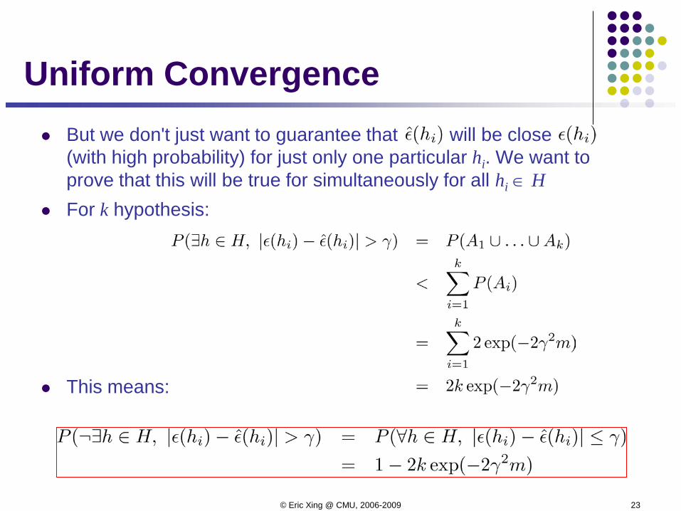
But we don't just want to guarantee that will be close (with high probability) for just only one particular hi. We want to prove that this will be true for simultaneously for all hi ∈ H

For k hypothesis:

This means:

Uniform Convergence

© Eric Xing @ CMU, 2006-2009 24

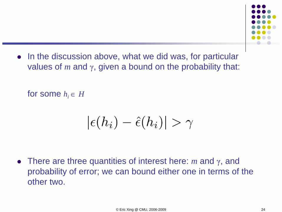
In the discussion above, what we did was, for particular values of m and γ, given a bound on the probability that:

for some hi ∈ H

There are three quantities of interest here: m and γ, and probability of error; we can bound either one in terms of the other two.

© Eric Xing @ CMU, 2006-2009 25

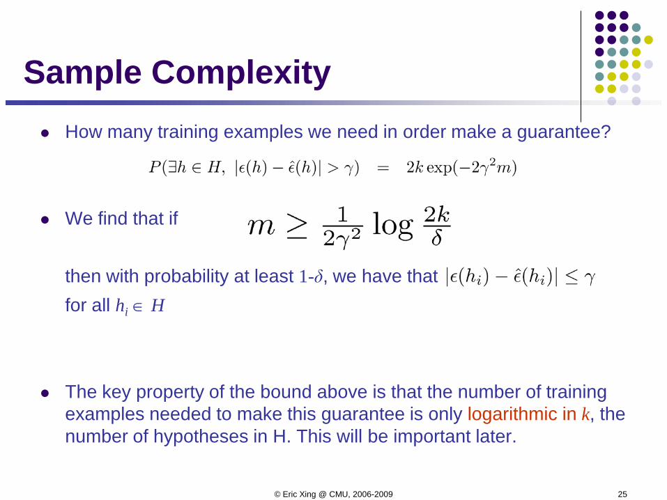
Sample Complexity How many training examples we need in order make a guarantee?

We find that if

then with probability at least 1-δ, we have thatfor all hi ∈ H

The key property of the bound above is that the number of training examples needed to make this guarantee is only logarithmic in k, the number of hypotheses in H. This will be important later.

© Eric Xing @ CMU, 2006-2009 26

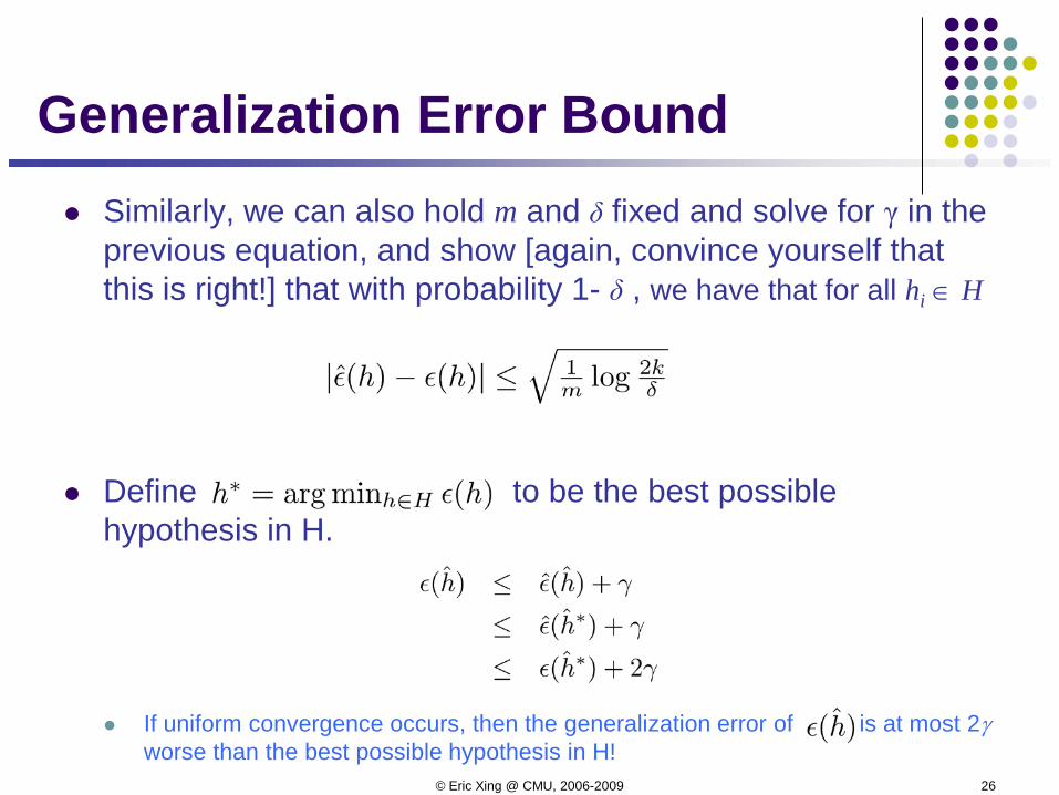
Generalization Error Bound Similarly, we can also hold m and δ fixed and solve for γ in the

previous equation, and show [again, convince yourself that this is right!] that with probability 1- δ , we have that for all hi ∈ H

Define to be the best possible hypothesis in H.

If uniform convergence occurs, then the generalization error of is at most 2γworse than the best possible hypothesis in H!

© Eric Xing @ CMU, 2006-2009 27

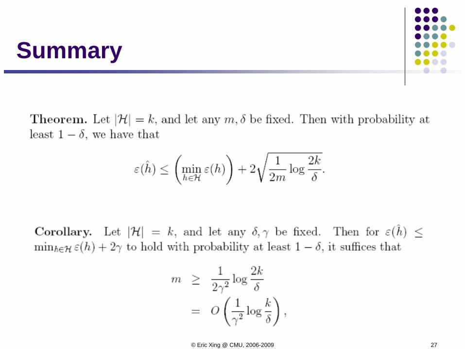
Summary

© Eric Xing @ CMU, 2006-2009 28

What if H is not finite? Can’t use our result for infinite H

Need some other measure of complexity for H– Vapnik-Chervonenkis (VC) dimension!

© Eric Xing @ CMU, 2006-2009 29

What if H is not finite? Some Informal Derivation

Suppose we have an H that is parameterized by d real numbers. Since we are using a computer to represent real numbers, and IEEE double-precision floating point (double's in C) uses 64 bits to represent a floating point number, this means that our learning algorithm, assuming we're using double-precision floating point, is parameterized by 64d bits

Parameterization

© Eric Xing @ CMU, 2006-2009 30

How do we characterize “power”? Different machines have different amounts of “power”. Tradeoff between:

More power: Can model more complex classifiers but might overfit. Less power: Not going to overfit, but restricted in what it can model

How do we characterize the amount of power?

© Eric Xing @ CMU, 2006-2009 31

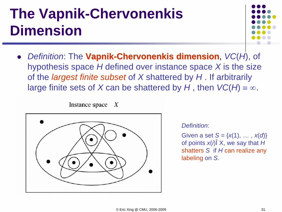
The Vapnik-Chervonenkis Dimension Definition: The Vapnik-Chervonenkis dimension, VC(H), of

hypothesis space H defined over instance space X is the size of the largest finite subset of X shattered by H . If arbitrarily large finite sets of X can be shattered by H , then VC(H) ≡ ∞.

Definition: Given a set S = {x(1), … , x(d)} of points x(i)Î X, we say that Hshatters S if H can realize any labeling on S.

© Eric Xing @ CMU, 2006-2009 32

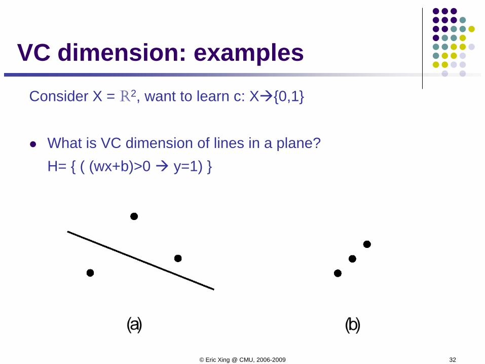
VC dimension: examplesConsider X = R2, want to learn c: X{0,1}

What is VC dimension of lines in a plane?H= { ( (wx+b)>0 y=1) }

© Eric Xing @ CMU, 2006-2009 33

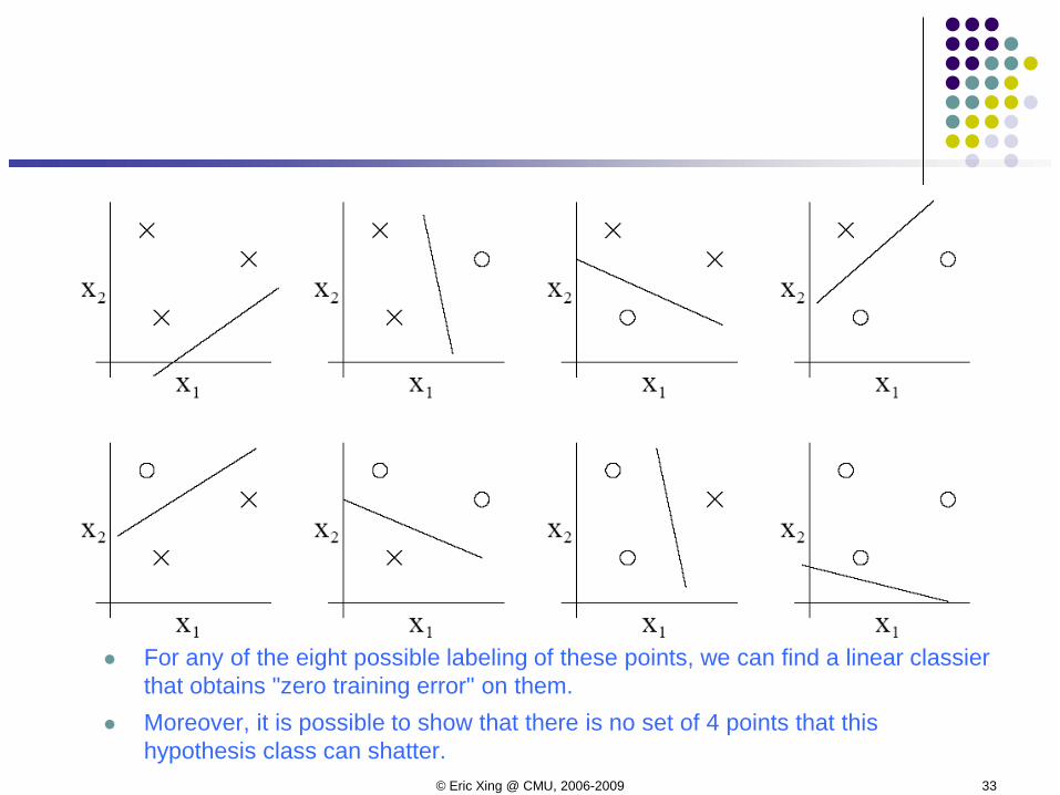
For any of the eight possible labeling of these points, we can find a linear classier that obtains "zero training error" on them.

Moreover, it is possible to show that there is no set of 4 points that this hypothesis class can shatter.

© Eric Xing @ CMU, 2006-2009 34

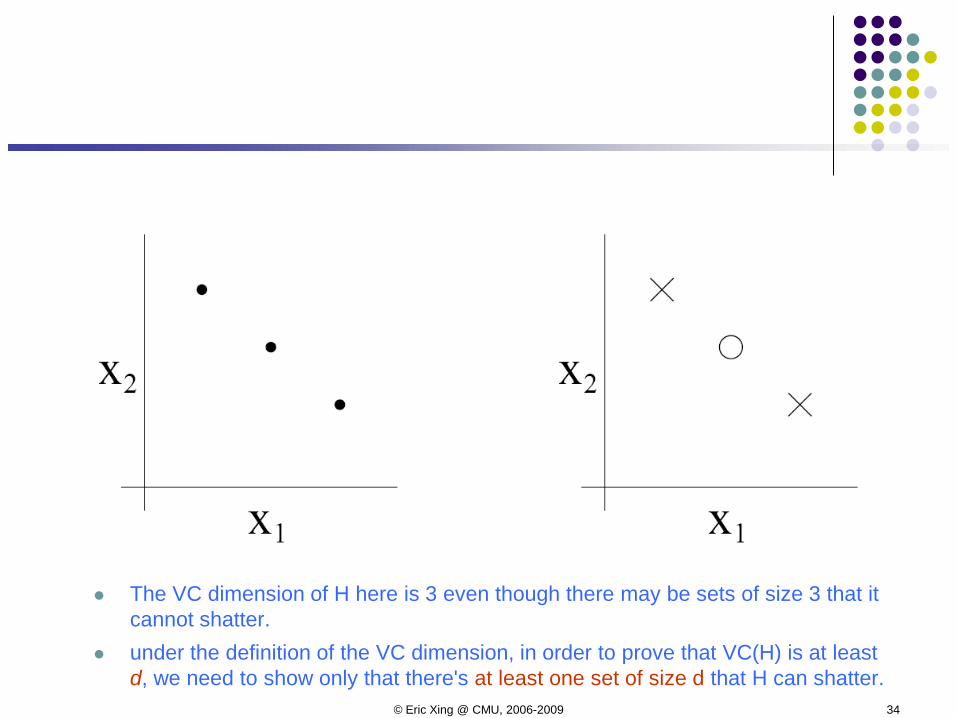
The VC dimension of H here is 3 even though there may be sets of size 3 that it cannot shatter.

under the definition of the VC dimension, in order to prove that VC(H) is at least d, we need to show only that there's at least one set of size d that H can shatter.

© Eric Xing @ CMU, 2006-2009 35

Theorem Consider some set of m points in Rn. Choose any one of the points as origin. Then the m points can be shattered by oriented hyperplanes if and only if the position vectors of the remaining points are linearly independent.

Corollary: The VC dimension of the set of oriented hyperplanes in Rn is n+1. Proof: we can always choose n + 1 points, and then choose one of the points as origin, such that the position vectors of the remaining n points are linearly independent, but can never choose n + 2 such points (since no n + 1 vectors in Rn can be linearly independent).

© Eric Xing @ CMU, 2006-2009 36

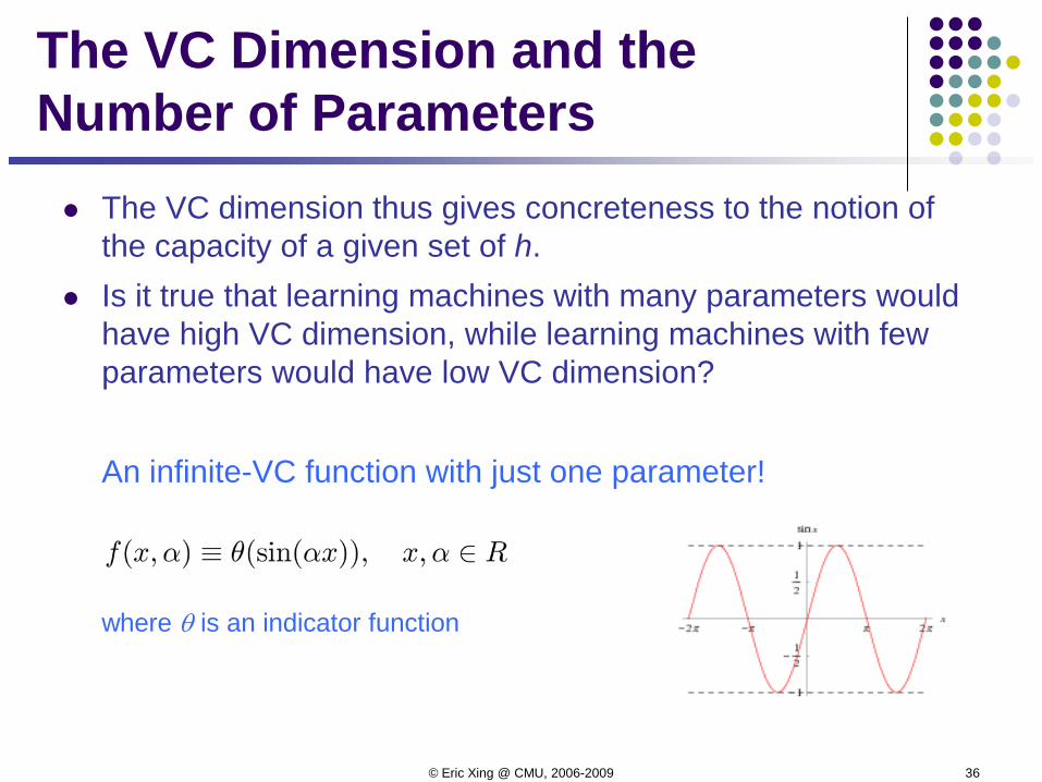
The VC Dimension and the Number of Parameters The VC dimension thus gives concreteness to the notion of

the capacity of a given set of h. Is it true that learning machines with many parameters would

have high VC dimension, while learning machines with few parameters would have low VC dimension?

An infinite-VC function with just one parameter!

where θ is an indicator function

© Eric Xing @ CMU, 2006-2009 37

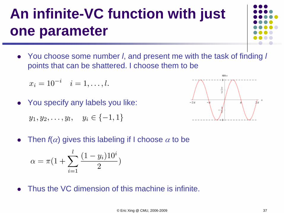
An infinite-VC function with just one parameter You choose some number l, and present me with the task of finding l

points that can be shattered. I choose them to be

You specify any labels you like:

Then f(α) gives this labeling if I choose α to be

Thus the VC dimension of this machine is infinite.

© Eric Xing @ CMU, 2006-2009 38

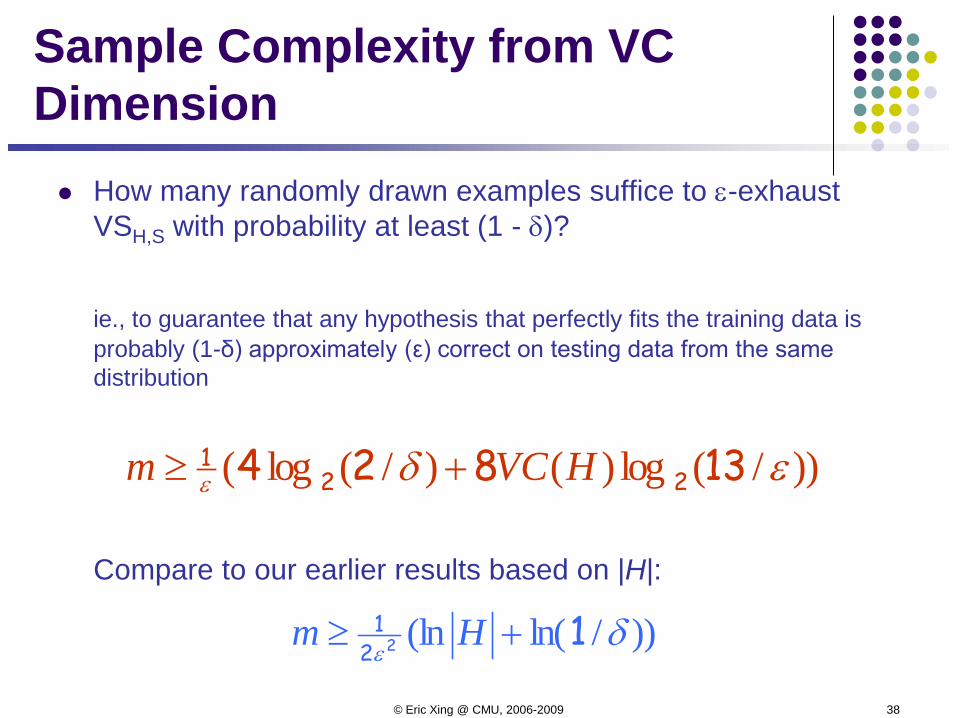
How many randomly drawn examples suffice to ε-exhaust VSH,S with probability at least (1 - δ)?

ie., to guarantee that any hypothesis that perfectly fits the training data is probably (1-δ) approximately (ε) correct on testing data from the same distribution

Compare to our earlier results based on |H|:

))/(log)()/(log( εδε 13824 221 HVCm +≥

Sample Complexity from VC Dimension

))/ln((ln δε

1221 +≥ Hm

© Eric Xing @ CMU, 2006-2009 39

What You Should Know Sample complexity varies with the learning setting

Learner actively queries trainer Examples provided at random

Within the PAC learning setting, we can bound the probability that learner will output hypothesis with given error For ANY consistent learner (case where c in H) For ANY “best fit” hypothesis (agnostic learning, where perhaps c not in H)

VC dimension as measure of complexity of H