UNIVERSITY OF CALIFORNIASanta Barbara
Image Steganalysis: Hunting & Escaping
A Dissertation submitted in partial satisfactionof the requirements for the degree of
Doctor of Philosophy
in
Electrical and Computer Engineering
by
Kenneth Mark Sullivan
Committee in Charge:
Professor Shivkumar Chandrasekaran, Co-Chair
Professor Upamanyu Madhow, Co-Chair
Professor B.S. Manjunath, Co-Chair
Professor Edward J. Delp
Doctor Ramarathnam Venkatesan
September 2005
The Dissertation ofKenneth Mark Sullivan is approved:
Professor Edward J. Delp
Doctor Ramarathnam Venkatesan
Professor Shivkumar Chandrasekaran, Committee Co-Chairman
Professor Upamanyu Madhow, Committee Co-Chairman
Professor B.S. Manjunath, Committee Co-Chairman
August 2005

Image Steganalysis: Hunting & Escaping
Copyright c© 2005
by
Kenneth Mark Sullivan
iii

To the memory of my sister, Kathleen
iv

Acknowledgements
I would like to thank the data hiding troika: Professors Manjunath, Madhow,
and Chandrasekaran. Prof. Manjunath taught me how to approach problems
and to keep an eye on the big picture. Prof. Madhow has a knack for explaining
difficult concepts concisely, and has helped me present my ideas more clearly.
Prof. Chandrasekaran always has an interesting new approach to offer, often
helping to push my thinking out of local minima. I also would like to think Prof.
Delp and Dr. Venkatesan for their time and helpful comments throughout this
research.
The research presented here was supported by the Office of Naval Research
(ONR #N00014-01-1-0380 and #N00014-05-1-0816), and the Center for Bioimage
Informatics at UCSB.
My data hiding colleague, Kaushal Solanki, has been great to work and travel
with over the past few years. During my research in the lab I have been lucky to
have a bright person in my field to bounce ideas off of and provide sanity checks,
literally just a few feet away. Onkar Dabeer was an amazing help, there seems to
be little he can not solve.
I will remember more of my years here than just sitting in the lab because of
my friends here. John, Tate, Christian, Noah, it’s been fun. GTA 100%, Ditch
Witchin’...lots of very exciting times occurred.
v

Jiyun, thanks for serving as my guide in Korea. Ohashi, thanks for your hos-
pitality in Japan. Dmiriti, thanks for translating Russian for me. To the rest of
the VRL, past and present: Sitaram, Marco, Baris, Shawn, Jelena, Motaz, Xind-
ing, Thomas, Feddo, and Maurits, I’ve learned at least as much from lunchtime
discussions as I did the rest of the day, I’m going to miss VRL. Judging from the
new kids: Nhat, Mary, Mike, and Laura, the future is in good hands.
Additionally, I would like to thank Prof. Ken Rose for providing a space for
me in signal compression lab to work in, and to the SCL members over the years:
Ashish, Ertem, Jaewoo, Jayanth, Hua, Sang-Uk, Pakpoom (thanks for the ride
home!), for making me feel at home there.
I owe a lot to fellow grad students outside my VRL/SCL world. Chowdary,
Chin, KGB, Vishi, Rich, Gwen, Suk-seung, thanks for the help and good times.
My friends from back in the day, Dave and Pete, you helped me take much
needed breaks from the whole grad school thing.
Finally I would like to thank my family. For the Brust clan, thanks for com-
miserating with us when Kaeding shanked that field goal. To my aunts Pat and
Susan, I am glad to have gotten to know you much better these past few years. My
brother Kevin and my parents Mike and Romaine Sullivan have been a constant
source of support; I always return from San Diego refreshed.
vi
Curriculum Vitæ
Kenneth Mark Sullivan
Education
2005 Doctor of Philosophy
Department of Electrical and Computer Engineering
University of California, Santa Barbara.
2002 Master of Science
Department of Electrical and Computer Engineering
University of California, Santa Barbara.
1998 Bachelor of Science
Department of Electrical and Computer Engineering
University of California, San Diego
Experience
2001 – 2005 Graduate Research Assistant,
University of California, Santa Barbara.
2001, 2005 Teaching Assistant, University of California, Santa Barbara.
1998 – 2000 Hardware/Software Engineer, Tiernan Communications Inc.,
San Diego.
1997 Intern, TRW Avionics Systems Division, San Diego.
vii
Selected Publications
K. Sullivan, U. Madhow, B. S. Manjunath, and S. Chandrase-
karan “Steganalysis for Markov Cover Data with Applications
to Images”, Submitted to IEEE Transactions on Information
Forensics and Security.
K. Solanki, K. Sullivan, B. S. Manjunath, U. Madhow, and S.
Chandrasekaran, “Statistical Restoration for Robust and Secure
Steganography”, To appear Proc. IEEE International Confer-
ence on Image Processing (ICIP), Genoa, Italy, Sep., 2005.
K. Sullivan, U. Madhow, S. Chandrasekaran and B. S. Manju-
nath, ”Steganalysis of Spread Spectrum Data Hiding Exploiting
Cover Memory” In Proc. IS&T/SPIE’s 17th Annual Symposium
on Electronic Imaging Science and Technology, San Jose, CA,
Jan. 2005.
O. Dabeer, K. Sullivan, U. Madhow, S. Chandrasekaran and B.S.
Manjunath, “Detection of Hiding in the Least Significant Bit”, In
IEEE Transactions on Signal Processing, Supplement on Secure
Media I, vol. 52, no. 10, pp. 3046–3058, Oct. 2004.
viii
K. Sullivan, Z. Bi, U. Madhow, S. Chandrasekaran and B.S.
Manjunath, “Steganalysis of quantization index modulation data
hiding”, In Proc. IEEE International Conference on Image Pro-
cessing (ICIP), Singapore, pp. 1165–1168, Oct. 2004.
K. Sullivan, O. Dabeer, U. Madow, B. S. Manujunath and S.
Chandrasekaran “LLRT Based Detection of LSB Hiding” In Proc.
IEEE International Conference on Image Processing (ICIP),
Barcelona, Spain, pp. 497–500, Sep. 2003
O. Dabeer, K. Sullivan, U. Madow, S. Chandrasekaran and B. S.
Manjunath “Detection of hiding in the least significant bit” In
Proc. Conference on Information Sciences and Systems (CISS)
Mar., 2003.
ix
Abstract
Image Steganalysis: Hunting & Escaping
Kenneth Mark Sullivan
Image steganography, the covert embedding of data into digital pictures, rep-
resents a threat to the safeguarding of sensitive information and the gathering
of intelligence. Steganalysis, the detection of this hidden information, is an in-
herently difficult problem and requires a thorough investigation. Conversely, the
hider who demands privacy must carefully examine a means to guarantee stealth.
A rigorous framework for analysis is required, both from the point of view of the
steganalyst and the steganographer. In this dissertation, we lay down a foundation
for a thorough analysis of steganography and steganalysis and use this analysis
to create practical solutions to the problems of detecting and evading detection.
Detection theory, previously employed in disciplines such as communications and
signal processing, provides a natural framework for the study of steganalysis, and
is the approach we take. With this theory, we make statements on the theoretical
detectability of modern steganography schemes, develop tools for steganalysis in a
practical scenario, and design and analyze a means of escaping optimal detection.
Under the commonly used assumption of an independent and identically dis-
tributed cover, we develop our detection-theoretic framework and apply it to the
x

steganalysis of LSB and quantization based hiding schemes. Theoretical bounds
on detection not available before are derived. To further increase the accuracy
of the model, we broaden the framework to include a measure of dependency
and apply this expanded framework to spread spectrum and perturbed quanti-
zation hiding methods. Experiments over a diverse database of images show our
steganalysis to be effective and competitive with the state-of-the-art.
Finally we shift focus to evasion of optimal steganalysis and analyze a method
believed to significantly reduce detectability while maintaining robustness. The
expected loss of rate incurred is analytically derived and it is shown that a high
volume of data can still be hidden.
xi
Contents
Acknowledgements v
Curriculum Vitæ vii
Abstract x
List of Figures xv
List of Tables xx
1 Introduction 11.1 Data Hiding Background . . . . . . . . . . . . . . . . . . . . . . . 21.2 Motivation . . . . . . . . . . . . . . . . . . . . . . . . . . . . . . . 41.3 Main Contributions . . . . . . . . . . . . . . . . . . . . . . . . . . 51.4 Notation, Focus, and Organization . . . . . . . . . . . . . . . . . 6
2 Steganography and Steganalysis 102.1 Basic Steganography . . . . . . . . . . . . . . . . . . . . . . . . . 102.2 Steganalysis . . . . . . . . . . . . . . . . . . . . . . . . . . . . . . 15
2.2.1 Detecting LSB Hiding . . . . . . . . . . . . . . . . . . . . 152.2.2 Detecting Other Hiding Methods . . . . . . . . . . . . . . 192.2.3 Generic Steganalysis: Notion of Naturalness . . . . . . . . 202.2.4 Evading Steganalysis . . . . . . . . . . . . . . . . . . . . . 232.2.5 Detection-Theoretic Analysis . . . . . . . . . . . . . . . . 29
2.3 Summary . . . . . . . . . . . . . . . . . . . . . . . . . . . . . . . 34
3 Detection-theoretic Approach to Steganalysis 363.1 Detection-theoretic Steganalysis . . . . . . . . . . . . . . . . . . . 36
xii
3.2 Least Significant Bit Hiding . . . . . . . . . . . . . . . . . . . . . 423.2.1 Statistical Model for LSB Hiding . . . . . . . . . . . . . . 423.2.2 Optimal Composite Hypothesis Testing for LSB Steganalysis 443.2.3 Asymptotic Performance of Hypothesis Tests . . . . . . . . 453.2.4 Practical Detection Based on LLRT . . . . . . . . . . . . . 493.2.5 Estimating the LLRT Statistic . . . . . . . . . . . . . . . . 503.2.6 LSB Hiding Conclusion . . . . . . . . . . . . . . . . . . . . 60
3.3 Quantization Index Modulation Hiding . . . . . . . . . . . . . . . 623.3.1 Statistical Model for QIM Hiding . . . . . . . . . . . . . . 633.3.2 Optimal Detection Performance . . . . . . . . . . . . . . . 673.3.3 Practical Detection . . . . . . . . . . . . . . . . . . . . . . 743.3.4 QIM Hiding Conclusion . . . . . . . . . . . . . . . . . . . 77
3.4 Summary . . . . . . . . . . . . . . . . . . . . . . . . . . . . . . . 78
4 Extending Detection-theoretic Steganalysis to Include Memory 794.1 Introduction . . . . . . . . . . . . . . . . . . . . . . . . . . . . . . 794.2 Detection Theory and Statistically Dependent Data . . . . . . . . 81
4.2.1 Detection-theoretic Divergence Measure for Markov Chains 814.2.2 Relation to Existing Steganalysis Methods . . . . . . . . . 87
4.3 Spread Spectrum . . . . . . . . . . . . . . . . . . . . . . . . . . . 904.3.1 Measuring Detectability of Hiding . . . . . . . . . . . . . . 904.3.2 Statistical Model for Spread Spectrum Hiding . . . . . . . 954.3.3 Practical Detection . . . . . . . . . . . . . . . . . . . . . . 994.3.4 SS Hiding Conclusion . . . . . . . . . . . . . . . . . . . . . 111
4.4 JPEG Perturbation Quantization . . . . . . . . . . . . . . . . . . 1114.4.1 Measuring Detectability of Hiding . . . . . . . . . . . . . . 1124.4.2 Statistical Model for Double JPEG Compressed PQ . . . . 114
4.5 Outguess . . . . . . . . . . . . . . . . . . . . . . . . . . . . . . . . 1174.6 Summary . . . . . . . . . . . . . . . . . . . . . . . . . . . . . . . 119
5 Evading Optimal Statistical Steganalysis 1235.1 Statistical Restoration Scheme . . . . . . . . . . . . . . . . . . . . 1255.2 Rate Versus Security . . . . . . . . . . . . . . . . . . . . . . . . . 128
5.2.1 Low Divergence Results . . . . . . . . . . . . . . . . . . . 1315.3 Hiding Rate for Zero K-L Divergence . . . . . . . . . . . . . . . . 133
5.3.1 Rate Distribution Derivation . . . . . . . . . . . . . . . . . 1335.3.2 General Factors Affecting the Hiding Rate . . . . . . . . . 1365.3.3 Maximum Rate of Perfect Restoration QIM . . . . . . . . 1385.3.4 Rate of QIM With Practical Threshold . . . . . . . . . . . 1435.3.5 Zero Divergence Results . . . . . . . . . . . . . . . . . . . 148
xiii
5.4 Hiding Rate for Zero Matrix Divergence . . . . . . . . . . . . . . 1505.4.1 Rate Distribution Derivation . . . . . . . . . . . . . . . . . 1505.4.2 Comparing Rates of Zero K-L and Zero Matrix DivergenceQIM . . . . . . . . . . . . . . . . . . . . . . . . . . . . . . . . . . 152
5.5 Summary . . . . . . . . . . . . . . . . . . . . . . . . . . . . . . . 156
6 Future Work and Conclusions 1586.1 Improving Model of Images . . . . . . . . . . . . . . . . . . . . . 1596.2 Accurate Characterization of Non-Optimal Detection . . . . . . . 1616.3 Summary . . . . . . . . . . . . . . . . . . . . . . . . . . . . . . . 162
Bibliography 164
A Glossary of Symbols and Acronyms 174
xiv

List of Figures
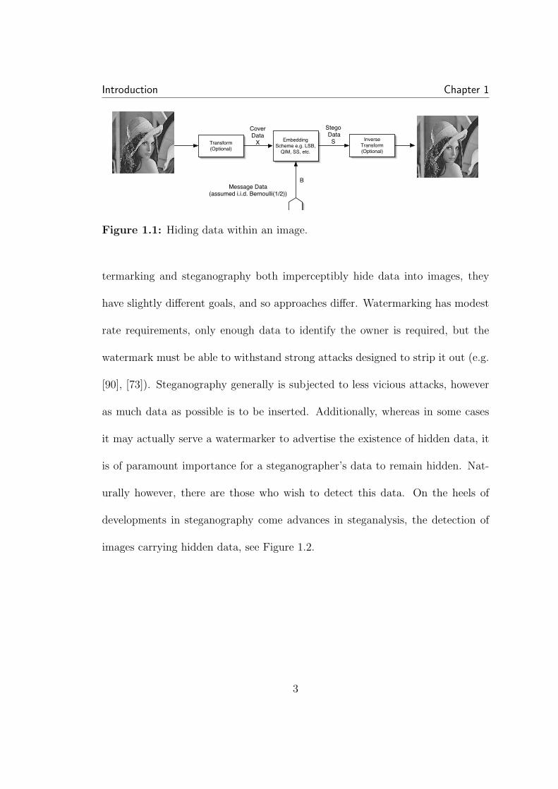
1.1 Hiding data within an image. . . . . . . . . . . . . . . . . . . . . 31.2 Steganalysis flow chart. . . . . . . . . . . . . . . . . . . . . . . . . 4
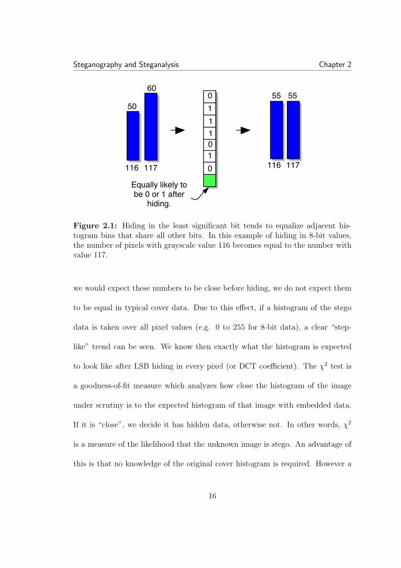
2.1 Hiding in the least significant bit tends to equalize adjacent his-togram bins that share all other bits. In this example of hiding in 8-bitvalues, the number of pixels with grayscale value 116 becomes equal tothe number with value 117. . . . . . . . . . . . . . . . . . . . . . . . . 16
3.1 Example of LSB hiding in the pixel values of an 8-bit grayscaleimage. . . . . . . . . . . . . . . . . . . . . . . . . . . . . . . . . . . . . 433.2 Unlike the LLRT, the χ2 (used in Stegdetect) threshold is sensitiveto the cover PMF . . . . . . . . . . . . . . . . . . . . . . . . . . . . . . 503.3 Approximate LLRT with half-half filter estimate versus χ2: for anythreshold choice, our approximate LLRT is superior. Each point on thecurve represents a fixed threshold. . . . . . . . . . . . . . . . . . . . . . 533.4 Hiding in the LSBs of JPEG coefficients: again LRT based methodis superior to χ2. . . . . . . . . . . . . . . . . . . . . . . . . . . . . . . 543.5 The rate that maximizes the LRT statistic (3.5) serves as an esti-mate of the hiding rate. . . . . . . . . . . . . . . . . . . . . . . . . . . 563.6 Here RS analysis, which uses cover memory, performs slightly bet-ter than the approximate LLRT. A hiding rate of 0.05 was used for alltest images with hidden data. . . . . . . . . . . . . . . . . . . . . . . . 583.7 Testing on color images embedded at maximum rate with S-tools.Because format conversion on some color images tested on causes his-togram artifacts that do not conform to our smoothness assumptions,performance is not as good as our testing on grayscale images. . . . . 59
xv
3.8 Conversion from one data format to another can sometimes causeidiosyncratic signatures, as seen in this example of periodic spikes in thehistogram. . . . . . . . . . . . . . . . . . . . . . . . . . . . . . . . . . . 603.9 Basic scalar QIM hiding. The message is hidden in choice of quan-tizer. For QIM designed to mimic non-hiding quantization (for com-pression for example) the quantization interval used for hiding is twicethat used for standard quantization. X is cover data, B is the bit to beembedded, S is the resulting stego data, and ∆ is the step-size of theQIM quantizers. . . . . . . . . . . . . . . . . . . . . . . . . . . . . . . 643.10 Dithering in QIM. The net statistical effect is to fill in the gapsleft behind by standard QIM, leaving a distribution similar, though notequal to, the cover distribution. . . . . . . . . . . . . . . . . . . . . . 653.11 The empirical PMF of the DCT values of an image. The PMFlooks not unlike a Laplacian, and has a large spike at zero. . . . . . . . 693.12 The detector is very sensitive to the width of the PMF versus thequantization step-size. . . . . . . . . . . . . . . . . . . . . . . . . . . . 713.13 Detection error as a function of the number of samples. The coverPMF is a Gaussian with (σ/∆) = 1 . . . . . . . . . . . . . . . . . . . . 73
4.1 An illustrative example of empirical matrices, here we have twobinary (i.e. Y = {0, 1}) 3 × 3 images. From each image a vector is cre-ated by scanning, and an empirical matrix is computed. The top imagehas no obvious interpixel dependence, reflected in a uniform empiri-cal matrix. The second image has dependency between pixels, as seenin the homogenous regions and so its empirical matrix has probabilityconcentrated along the main diagonal. Though the method of scanning(horizontal, vertical, zig-zag) has a large effect on the empirical matrixin this contrived example, we find the effect of the scanning method onreal images to be small. . . . . . . . . . . . . . . . . . . . . . . . . . . 844.2 Empirical matrices of SS globally adaptive hiding. The convolu-tion of a white Gaussian empirical matrix (bell-shaped) with an imageempirical matrix (concentrated at the main diagonal) results in a newstego matrix less concentrated along the main diagonal. In other words,the hiding weakens dependencies. . . . . . . . . . . . . . . . . . . . . . 964.3 Global (left) and local (right) hiding both have similar effects, aweakening of dependencies as seen as a shift out from the main diagonal.However the effect is more pronounced with globally adaptive hiding. . 98
xvi
4.4 An example of the feature vector extraction from an empiricalmatrix (not to scale). Most of the probability is concentrated in thecircled region. Six row segments are taken at high probabilities alongthe main diagonal and the main diagonal itself is subsampled. . . . . . 1034.5 The feature vector on the left is derived from the empirical matrixand captures the changes to interdependencies caused by SS data hiding.The feature vector on the right is the normalized histogram and onlycaptures changes to first order statistics, which are negligible. . . . . . 1044.6 ROCs of SS detectors based on empirical matrices (left) and one-dimensional histograms (right). In all cases detection is much better forthe detector including dependency. For this detector (left), the globallyadaptive schemes can be seen to be more easily detected than locallyadaptive schemes. Additionally, spatial and DCT hiding rates are nearlyidentical for globally adaptive hiding, but differ greatly for locally adap-tive hiding. In all cases detection is better than random guessing. Theglobally adaptive schemes achieve best error rates of about 2-3% forP(false alarm) and P(miss). . . . . . . . . . . . . . . . . . . . . . . . . 1054.7 Detecting locally adaptive DCT hiding with three different super-vised learning detectors. The feature vectors are derived from empiri-cal matrices calculated from three separate scanning methods: vertical,horizontal, and zigzag. All perform roughly the same. . . . . . . . . . . 1064.8 ROCs for locally adaptive hiding in the transform domain (left)and spatial domain (right). All detectors based on combined featuresperform about the same for transform domain hiding. For spatial do-main hiding, the cut-and-paste performs much worse. . . . . . . . . . . 1084.9 A comparison of detectors for locally adaptive DCT spread spec-trum hiding. The two empirical matrix detectors, one using one ad-jacent pixel and the other using an average of a neighborhood aroundeach pixel, perform similarly. . . . . . . . . . . . . . . . . . . . . . . . 1104.10 On the left is an empirical matrix of DCT coefficients after quanti-zation. When decompressed to the spatial domain and rounded to pixelvalues, right, the DCT coefficients are randomly distributed around thequantization points. . . . . . . . . . . . . . . . . . . . . . . . . . . . . 115
xvii
4.11 A simplified example of second compression on an empirical ma-trix. Solid lines are the first quantizer intervals, dotted lines the second.The arrows represent the result of the second quantization. The den-sity blurring after decompression is represented by the circles centeredat the quantization points. For the density at (84,84), if the density issymmetric, the values are evenly distributed to the surrounding pairs.If however there is an asymmetry, such as the dotted ellipse, the newdensity favors some pairs over others (e.g. (72,72), (96,96) over (72,96),(96,72). The effect is similar for other splits such as (63,84) to (72,72)and (72,96). . . . . . . . . . . . . . . . . . . . . . . . . . . . . . . . . . 1164.12 Detector performance of Outguess using classifier trained on de-pendency statistics. . . . . . . . . . . . . . . . . . . . . . . . . . . . . . 119
5.1 Rate, security tradeoff for Gaussian cover with σ/∆ of 1. As ex-pected, compensating is a more efficient means of increasing securitywhile reducing rate. . . . . . . . . . . . . . . . . . . . . . . . . . . . . . 1315.2 Each realization of a random process has a slightly different his-togram. The distribution of the number of elements in each bin is bi-nomially distributing according to the expected value of the bin center(i.e. the integral of the pdf over the bin). . . . . . . . . . . . . . . . . . 1355.3 The pdf of Γ, the ratio limiting our hiding rate, for each bin i.The expected Γ drops as one moves away from the center. Additionally,at the extremes, e.g. ±4, the distribution is not concentrated. In thisexample, N = 50000, σ/∆ = 0.5, and w = 0.05. . . . . . . . . . . . . . 1405.4 The expected histogram of the stego coefficients is a smoothed
version of the original. Therefore the ratioP E
X [i]
P ES [i]
is greater than one in
the center, but drops to less than one for higher magnitude values. . . 1415.5 A larger threshold allows a greater number of coefficients to be em-bedded. This partially offsets the decrease in expected λ∗ with increasedthreshold. . . . . . . . . . . . . . . . . . . . . . . . . . . . . . . . . . . 1445.6 On the left is an example of finding the 90%-safe λ for a thresholdof 1.3. On the right is safe λ for all thresholds, with 1.3 highlighted. . . 1455.7 Finding the best rate. By varying the threshold, we can find thebest tradeoff between λ and the number of coefficients we can hide in. 1465.8 A comparison of the expected histograms for a threshold of one(left) and two (right). Though the higher threshold densitie appears tobe closer to the ideal case, the minimum ratio PX/PS is lower in this case. 147
xviii
5.9 The practical case: Γ density over all bins within the thresholdregion, for a threshold of two. Though for bins immediately before thethreshold, Γ is high, the expected Γ drops quickly after this. As before,N = 50000, σ/∆ = 0.5, and w = 0.05. . . . . . . . . . . . . . . . . . . 1485.10 A comparison of practical detection in real images. As expected,after perfect restoration, detection is random, though non-restored hid-ing at the same rate is detectable. . . . . . . . . . . . . . . . . . . . . . 1495.11 A comparison of the rates guaranteeing perfect marginal and jointhistogram restoration 90% of the time. Correlation does not affect themarginal statistics, so the rate is constant. All factors other than ρ areheld constant: N = 10000, w = 0.1, σX = 1, ∆ = 2. Surprisingly,compensating the joint histogram can achieve higher rates than themarginal histogram. . . . . . . . . . . . . . . . . . . . . . . . . . . . . 155
xix
List of Tables
3.1 If the design quality factor is constant (set at 50), a very lowdetection error can be achieved at all final quality levels. Here ‘0’ meansno errors occurred in 500 tests so the error rate is < 0.002 . . . . . . . 763.2 In a more realistic scenario where the design quality factor is un-known, the detection error is higher than if it is known, but still suf-ficiently low for some applications. Also, the final JPEG compressionplays an important role. As compression becomes more severe, the de-tection becomes less accurate. . . . . . . . . . . . . . . . . . . . . . . . 77
4.1 Divergence measurements of spread spectrum hiding (all valuesare multiplied by 100). As expected, the effect of transform and spatialhiding is similar. There is a clear gain here for the detector to usedependency. A factor of 20 means the detector can use 95% less samplesto achieve the same detection rates. . . . . . . . . . . . . . . . . . . . 934.2 For SS locally adaptive hiding, the calculated divergence is relatedto the cover medium, with DCT hiding being much lower. Additionallythe detector gain is less for DCT hiding. . . . . . . . . . . . . . . . . . 944.3 A comparison of the classifier performance based on comparingthree different soft decision statistics to a zero threshold: the output of aclassifier using a feature vector derived from horizontal image scanning;the output of a classifier using the cut-and-paste feature vector describedabove, and the sum of these two. In this particular case, adding thesoft classifier output before comparing to zero threshold achieves betterdetection than either individual case. . . . . . . . . . . . . . . . . . . 109
xx
4.4 Divergence measures of PQ hiding (all values are multiplied by100). Not surprisingly, the divergence is greater comparing to a twicecompressed cover than a single compressed cover, matching the findingsof Kharrazi et al. The divergence measures on the right (comparing toa double-compressed cover) are about half that of the locally adaptiveDCT SS case in which detection was difficult, helping to explain thepoor detection results. . . . . . . . . . . . . . . . . . . . . . . . . . . . 113
5.1 It can be seen that statistical restoration causes a greater numberof errors for the steganalyst. In particular for standard hiding, thesum of errors for the compensated case is more than twice that theuncompensated. . . . . . . . . . . . . . . . . . . . . . . . . . . . . . . . 1325.2 An example of the derivation of maximum 90%-safe rate for prac-tical integer thresholds. Here the best threshold is T = 1 with λ = 0.45There is no 90%-safe λ for T = 3, so the rate is effectively zero. . . . . 149
xxi
Chapter 1
Introduction
Image steganography, the covert embedding of data into digital pictures, rep-
resents a threat to the safeguarding of sensitive information and the gathering
of intelligence. Steganalysis, the detection of this hidden information, is an in-
herently difficult problem and requires a thorough investigation. Conversely, the
hider who demands privacy must carefully examine a means to guarantee stealth.
A rigorous framework for analysis is required, both from the point of view of the
steganalyst and the steganographer.
The main contribution of this work is the development of a foundation for the
thorough analysis of steganography and steganalysis and the use of this analysis
to create practical solutions to the problems of detecting and evading detection.
Image data hiding is a field that lies in the intersection of communications and
image processing, so our approach employs elements of both areas. Detection
theory, employed in disciplines such as communications and signal processing,
1

Introduction Chapter 1
provides a natural framework for the study of steganalysis. Image processing
provides the theory and tools necessary to understand the unique characteristics
of cover images. Additionally, results from fields such as information theory and
pattern recognition are employed to advance the study.
1.1 Data Hiding Background
As long as people have been able to communicate with one another, there has
been a desire to do so secretly. Two general approaches to covert exchanges of
information have been: communicate in a way understandable by the intended
parties, but unintelligible to eavesdroppers; or communicate innocuously, so no
extra party bothers to eavesdrop. Naturally both of these methods can be used
concurrently to enhance privacy. The formal studies of these methods, cryptogra-
phy and steganography, have evolved and become increasingly more sophisticated
over the centuries to the modern digital age. Methods for hiding data into cover
or host media, such as audio, images, and video, were developed about a decade
ago (e.g. [89], [101]). Although the original motivation for the early development
of data hiding was to provide a means of “watermarking” media for copyright pro-
tection [58], data hiding methods were quickly adapted to steganography [2, 55].
See Figure 1.1 for a schematic of an image steganography system. Although wa-
2
Introduction Chapter 1
Transform (Optional)
Embedding Scheme e.g. LSB,
QIM, SS, etc.
Cover Data
X
Stego Data
S
BMessage Data
(assumed i.i.d. Bernoulli(1/2))
InverseTransform (Optional)
Figure 1.1: Hiding data within an image.
termarking and steganography both imperceptibly hide data into images, they
have slightly different goals, and so approaches differ. Watermarking has modest
rate requirements, only enough data to identify the owner is required, but the
watermark must be able to withstand strong attacks designed to strip it out (e.g.
[90], [73]). Steganography generally is subjected to less vicious attacks, however
as much data as possible is to be inserted. Additionally, whereas in some cases
it may actually serve a watermarker to advertise the existence of hidden data, it
is of paramount importance for a steganographer’s data to remain hidden. Nat-
urally however, there are those who wish to detect this data. On the heels of
developments in steganography come advances in steganalysis, the detection of
images carrying hidden data, see Figure 1.2.
3
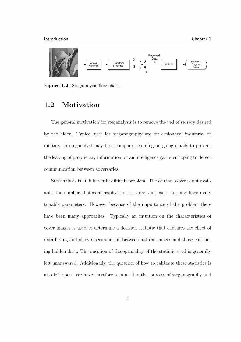
Introduction Chapter 1
?
X
SY Detector
Received Data
Decision: Stego or
CoverTransform(if needed)
Attack(Optional)
Figure 1.2: Steganalysis flow chart.
1.2 Motivation
The general motivation for steganalysis is to remove the veil of secrecy desired
by the hider. Typical uses for steganography are for espionage, industrial or
military. A steganalyst may be a company scanning outgoing emails to prevent
the leaking of proprietary information, or an intelligence gatherer hoping to detect
communication between adversaries.
Steganalysis is an inherently difficult problem. The original cover is not avail-
able, the number of steganography tools is large, and each tool may have many
tunable parameters. However because of the importance of the problem there
have been many approaches. Typically an intuition on the characteristics of
cover images is used to determine a decision statistic that captures the effect of
data hiding and allow discrimination between natural images and those contain-
ing hidden data. The question of the optimality of the statistic used is generally
left unanswered. Additionally, the question of how to calibrate these statistics is
also left open. We have therefore seen an iterative process of steganography and
4

Introduction Chapter 1
steganalysis: a steganographic method is detected by a steganalysis tool, a new
steganographic method is invented to prevent detection, which in turn is found to
be susceptible to an improved steganalysis. It is not known then what the limits
of steganalysis are, an important question for both the steganographer and ste-
ganalyst. It is hoped by careful analysis that some measure of optimal detection
can be obtained.
1.3 Main Contributions
• Detection-theoretic Framework. Detection theory is well-developed
and is naturally suited to the steganalysis problem. We develop a detection-
theoretic approach to steganalysis general enough to estimate the perfor-
mance of theoretically optimal detection yet detailed enough to help guide
the creation of practical detection tools [21, 85, 20].
• Practical Detection of Hiding Methods. In practice, not enough infor-
mation is available to use optimal detection methods. By devising methods
of estimating this information from either the received data, or through su-
pervised learning, we created methods that practically detect three general
classes of data hiding: least significant bit (LSB) [21, 85, 20], quantization
5
Introduction Chapter 1
index modulation (QIM) [84], and spread spectrum (SS) [87, 86]. These
methods compare favorably with published detection schemes.
• Expand Detection-theoretic Approach to Include Dependencies.
Typically analysis of the steganalysis problem has used an independent and
identically distributed (i.i.d.) assumption. For practical hiding media, this
assumption is too simple. We take the next logical step and augment the
analysis by including Markov chain data, adding statistically dependent
data to the detection-theoretic approach [87, 86].
• Evasion of Optimal Steganalysis. From our work on optimal steganal-
ysis, we have learned what is required to escape detection. We use our
framework to guide evasion efforts and successfully reduce the effectiveness
of previously successful detection for dithered QIM [82]. This analysis is
also used to derive a formulation of the rate of secure hiding for arbitrary
cover distributions.
1.4 Notation, Focus, and Organization
We refer to original media with no hidden data as cover media, and media
containing hidden data as stego media (e.g. cover images, stego transform co-
efficients). The terms hiding or embedding are used to denote the process of
6
Introduction Chapter 1
adding hidden data to an image. We use the term robust to denote the abil-
ity of a data hiding scheme to withstand changes incurred to the image be-
tween the sender and intended receiver. These changes may be from a mali-
cious attack, transmission noise, or common image processing transformations,
most notably compression. By detection, we mean that a steganalyst has cor-
rectly classified a stego image as containing hidden data. Decoding is used to
denote the reception of information by the intended receiver. We use secure in
the steganographic sense, meaning safe from detection by steganalysis. We use
capital letters to denote a random variable, and lower case letters to denote the
value of its realization. Boldface indicates vectors (lower case) and matrices (up-
per case). For probability mass functions we use either vector/matrix notation:
p(X) : p(X)i = P (X = i), M
(X)ij = P (X1 = i, X2 = j) or function notation:
PX(x) = P (X = x), PX1,X2(x1, x2) = P (X1 = x1, X2 = x2) where context deter-
mines which is more convenient. A complete list of symbols and acronyms used
is provided in the Appendix.
Classification between cover and stego is often referred to as “passive” ste-
ganalysis while extracting hidden information is referred to as “active” steganal-
ysis. Extraction can also be used as an attack on a watermarking system: if the
watermark is known, it can easily be removed without distorting the cover image.
In most cases, the extraction is actually a special case of cryptanalysis (e.g. [62]),
7
Introduction Chapter 1
a mature field in its own right. We focus exclusively on passive steganalysis and
drop the term “passive” where clear. To confuse matters, the literature also often
refers to a “passive” and “active” warden. In both cases, the warden controls
the channel between the sender and receiver. A passive warden lets an image
pass through unchanged if it is judged to not contain hidden data. An active
warden attempts to destroy any possible hidden data by making small changes to
the image, similar in spirit to a copyright violator attempting to remove a water-
mark. We generally focus on the passive warden scenario, since many aspects of
the active warden case are well studied in watermarking research. However, we
discuss the robustness of various hiding methods to an active warden and other
possible attacks/noise.
Furthermore, though data hiding techniques have been developed for audio,
image, video, and even non-multimedia data sources such as software [91], we fo-
cus on digital images. Digital images are well suited to data hiding for a number
of reasons. Images are ubiquitous on the Internet; posting an image on a web-
site or attaching a picture to an email attracts no attention. Even with modern
compression techniques, images are still relatively large and can be changed im-
perceptibly, both important for covert communication. Finally there exist several
well-developed methods for image steganography, more than for any other data
hiding medium. We focus on grayscale images in particular.
8

Introduction Chapter 1
To provide context for our examination of steganalysis, in the following chapter
we review steganography and steganalysis research presented in the literature. In
Chapter 3, we explain the detection-theoretic framework we use throughout the
study, and apply it to the steganalysis of LSB and QIM hiding schemes. In
Chapter 4, we broaden the framework to include a measure of dependency and
apply this expanded framework to SS and PQ hiding methods. In Chapter 5, we
shift focus to evasion of optimal steganalysis and analyze a method believed to
significantly reduce detectability while maintaining adequate rate and robustness.
We summarize our conclusions and discuss future research directions in Chapter 6.
9

Chapter 2
Steganography and Steganalysis
We here survey the concurrent development of image steganography and ste-
ganalysis. Research and development of steganography preceded steganalysis,
and steganalysis has been forced to catch up. More recently, steganalysis has
had some success and steganographers have had to more carefully consider the
stealthiness of their hiding methods.
2.1 Basic Steganography
Digital image steganography grew out of advances in digital watermarking.
Two early watermarking methods which became two early steganographic meth-
ods are: overwriting the least significant bit (LSB) plane of an image with a
message; and adding a message bearing signal to the image [89].
The LSB hiding method has the advantage of simplicity of encoding, and a
guaranteed successful decoding if the image is unchanged by noise or attack. How-
10

Steganography and Steganalysis Chapter 2
ever the LSB method is very fragile to any attack, noise, or even standard image
processing such as compression [52]. Additionally, because the least significant
bit plane is overwritten, the data is irrecoverably lost. For the steganographer,
however, there are many scenarios with which the image remains untouched, and
the cover image can be considered disposable. As such, LSB hiding is still very
popular today; a perusal of tools readily available online reveals numerous LSB
embedding software packages [74]. We examine LSB hiding in greater detail in
Chapter 3.
The basic idea of additive hiding is straightforward. Typically the binary mes-
sage modulates a sequence known by both encoder and decoder, and this is added
to the image. This simplicity lends itself to adaptive improvements. In particular,
unlike LSB, additive hiding schemes can be designed to withstand changes to the
image such as JPEG compression and noise [101]. Additionally, if the decoder
correctly receives the message, he or she can simply subtract out the message
sequence, recovering the original image (assuming no noise or attack). Much
watermarking research then has focused on additive hiding schemes, specifically
improving robustness to malicious attacks (e.g. [73],[90]) deliberately designed to
remove the watermark.
A commonly used adaptation of the additive hiding scheme is the spread
spectrum (SS) method introduced by Cox et al [19]. As suggested by the name,
11

Steganography and Steganalysis Chapter 2
the message is spread (whitened) as is typically done in many applications such as
wireless communications and anti-jam systems [66], and then added to the cover.
This method, with various adaptations, can be made robust to typical geometric
and noise adding attacks. Naturally newer attacks are created (e.g. [62]) and new
solutions to the attacks are proposed. As with LSB hiding, spread spectrum and
close variants are also used for steganography [60, 31]. We describe SS hiding in
greater detail in Chapter 4.
An inherent problem with SS hiding, and any additive hiding, is interference
from the cover medium. This interference can cause errors at the decoder, or
equivalently, lowers the amount of data that can be accurately received. However,
the hider has perfect knowledge of the interfering cover; surely the channel has a
higher capacity than if the interference were unknown. Work done by Gel’Fand
and Pinsker [39], as well as Costa [17], on hiding in a channel with side information
known only by the encoder show that the capacity is not effected by the known
noise at all. In other words, if the data is encoded correctly by the hider, there
is effectively no interference from the cover, and the decoder only needs to worry
about outside noise or attacks. The encoder used by Costa for his proof is not
readily applicable. However, for the data hiding problem, Chen and Wornell
proposed quantization index modulation QIM [14] to avoid cover interference.
This coding method and its variants achieve, or closely achieve, the capacity
12
Steganography and Steganalysis Chapter 2
predicted by Costa. The basic idea is to hide the message data into the cover
by quantizing the cover with a choice of quantizer determined by the message.
The simplest example is so-called odd/even embedding. With this scheme, a
continuous valued cover sample is used to embed a single bit. To embed a 0, the
cover sample is rounded to the nearest even integer, to embed a 1, round to the
nearest odd number. The decoder, with no knowledge of the cover, can decode
the message so long as perturbations (from noise or attack) do not change the
values by more than 0.5. Other similar approaches have been proposed such as
the scalar Costa scheme (SCS) by Eggers et al [25]. This class of embedding
techniques is sometimes referred to as quantization-based techniques, dirty paper
codes (from the title of Costa’s paper), and binning methods [104]; we use the
term QIM. As the expected capacity is higher than the host interference case,
QIM is well suited for steganographic methods [81, 54]. This hiding technique in
described in greater detail in Chapter 3.
All of the above methods can be performed in the spatial domain (i.e. pixel val-
ues) or in some transform domain. Popular transforms include the two-dimensional
discrete cosine transform (DCT), discrete Fourier transform (DFT) [50] and dis-
crete wavelet transforms (DWT) [92]. These transforms may be performed block-
wise, or over the entire image. For a blockwise transform, the image is broken
into smaller blocks (8× 8 and 16× 16 are two popular sizes), and the transform
13
Steganography and Steganalysis Chapter 2
is performed individually on each block. The advantage of using transforms is
that it is generally easier to balance distortion introduced by hiding and robust-
ness to noise or attack in the transform domain then in the pixel domain. These
transforms can in principle be used with any hiding scheme. LSB hiding however
requires digitized data, so continuous valued transform coefficients must be quan-
tized. Transform LSB hiding is therefore generally limited to compressed (with
JPEG [94] for example) images, in which the transform coefficients are quantized.
Additionally, QIM has historically been used much more often in the transform
domain.
We have then three main categories of hiding methods: LSB, SS, and QIM.
Data hiding is an active field with new methods constantly introduced, and cer-
tainly some of these do not fit into these three categories. However the three
we focus on are the most commonly used today, and provide a natural starting
point for study. In addition to immediately applicable results, it is hoped that the
analysis of these schemes yields findings adaptable to future developments. We
now examine some of the steganalysis methods introduced over the last decade
to detect these schemes, particularly the popular LSB method. Steganography
research has not been idle, and we also review the hider’s response to steganalysis.
14
Steganography and Steganalysis Chapter 2
2.2 Steganalysis
There is a myriad of approaches to the steganalysis problem. Since the gen-
eral steganalysis problem, discriminating between images with hidden data and
images without, is very broad, some assumptions are made to obtain a well-posed
problem. Typically these assumptions are made on the cover data, the hiding
method, or both. Each steganalysis method presented here uses a different set
of assumptions; we look at the advantages and disadvantages of these various
approaches.
2.2.1 Detecting LSB Hiding
An early method used to detect LSB hiding is the χ2 (chi-squared) technique
[100], later successfully used by Provos’ stegdetect [69] for detection of LSB hiding
in JPEG coefficients. We first note that generally the binary message data is
assumed to be i.i.d. with the probability of 0 equality to the probability of 1. If the
hider’s intended message does not have these properties, a wise steganographer
would use an entropy coder to reduce the size of the message; the compressed
version of the message should fulfill the assumptions. Because 0 and 1 are equally
likely, after overwriting the LSB, it is expected that the number of pixels in a pair
of values which share all but the LSB are equalized, see Figure 2.1. Although
15
Steganography and Steganalysis Chapter 2
50
60
116 117 116 117
55 550
0
0
111
1
Equally likely to be 0 or 1 after
hiding.
Figure 2.1: Hiding in the least significant bit tends to equalize adjacent his-togram bins that share all other bits. In this example of hiding in 8-bit values,the number of pixels with grayscale value 116 becomes equal to the number withvalue 117.
we would expect these numbers to be close before hiding, we do not expect them
to be equal in typical cover data. Due to this effect, if a histogram of the stego
data is taken over all pixel values (e.g. 0 to 255 for 8-bit data), a clear “step-
like” trend can be seen. We know then exactly what the histogram is expected
to look like after LSB hiding in every pixel (or DCT coefficient). The χ2 test is
a goodness-of-fit measure which analyzes how close the histogram of the image
under scrutiny is to the expected histogram of that image with embedded data.
If it is “close”, we decide it has hidden data, otherwise not. In other words, χ2
is a measure of the likelihood that the unknown image is stego. An advantage of
this is that no knowledge of the original cover histogram is required. However a
16
Steganography and Steganalysis Chapter 2
weakness of the χ2 test is that it only says how likely the received data is stego,
it does not say how likely it is cover. A better test is to decide if it is closer
to stego than to cover, otherwise an arbitrary choice must be made as to when
it is far enough to be considered clean. We explore the cost of this more fully
in Chapter 3. In practice the χ2 test works reasonably well in discriminating
between cover and stego. The χ2 is an example of an early approach to detecting
changes using the statistics of an image, in this case using an estimate of the
probability distribution, i.e. a histogram. Previous detection methods were often
visual, i.e. for some hiding methods it was found that, in some domain, the hiding
was actually recognizable by the naked eye. Visual attacks are easily compensated
for, but statistical detection is more difficult to thwart.
Another LSB detection scheme was proposed by Avcibas et al [4] using binary
similarity measures between the 7th bit plane and the 8th (least significant) bit
plane. It is assumed that there is a natural correlation between the bit planes
that is disrupted by LSB hiding. This scheme does not auto-calibrate on a per
image basis, and instead calibrates on a training set of cover and stego images.
The scheme works better than a generic steganalysis scheme, but not as well as
state-of-the-art LSB steganalysis.
Two more recent and powerful LSB detection methods are the RS (regu-
lar/singular) scheme [33] and the related sample pair analysis [24]. The RS
17
Steganography and Steganalysis Chapter 2
scheme, proposed by Fridrich et al, is a specific steganalysis method for detecting
LSB data hiding in images. Sample pair analysis is a more rigorous analysis due
to Dumitrescu et al of the basis of the RS method, explaining why and when it
works. The sample pairs are any pair of values (not necessarily consecutive) in
a received sequence. These pairs are partitioned into subsets depending on the
relation of the two values to one another. Is is assumed that in a cover image the
number of pairs in each subset are roughly equal. It is shown that LSB hiding
performs a different function on each subset, and so the number of pairs in the
subsets are not equal. The amount of disruption can be measured and related to
the known effect of LSB hiding to estimate the rate of hiding. Although the initial
assumption does not require interpixel dependencies, it can be shown that corre-
lated data provides stronger estimates than uncorrelated data. The RS scheme,
a practical detector of LSB data hiding, uses the same basic principle as sample
pair analysis. As in sample pair analysis, the RS scheme counts the number of
occurrences of pairs in given sets. The relevant sets, regular and singular (hence
RS), are related to but slightly different from the sets used in sample pair analysis.
Also as in sample pair analysis, equations are derived to estimate the length of
hidden messages. Since RS employs the same principle as sample pair analysis,
we would expect it to also work better for correlated cover data. Indeed the RS
scheme focuses on spatially adjacent image pixels, which are known to be highly
18
Steganography and Steganalysis Chapter 2
correlated. In practice RS analysis and sample pair analysis perform compara-
bly. Recently Roue et al [72] use estimates of the joint probability mass function
(PMF) to increase the detection rate of RS/sample pair analysis. We explore
the joint PMF estimate in greater detail in Chapter 4. A recent scheme, also by
Fridrich and Goljan [32], uses local estimators based on pixel neighborhoods to
slightly improve LSB detection over RS.
2.2.2 Detecting Other Hiding Methods
Though most of the focus of steganalysis has been on detecting LSB hiding,
other methods have also been investigated.
Harmsen and Pearlman studied [45] the steganalysis of additive hiding schemes
such as spread spectrum. Their decision statistic is based initially on a PMF es-
timate, i.e. a histogram. Since additive hiding is an addition of two random
variables: the cover and the message sequence, the PMF of cover and message
sequences are convolved. In the Fourier domain, this is equivalent to multiplica-
tion. Therefore the DFT of the histogram, termed the histogram characteristic
function (HCF), is taken. It is shown for typical cover distributions that the ex-
pected value, or center of mass (COM), of the HCF does not increase after hiding,
and in practice typically decreases. The authors choose then to use the COM as
a feature to train a Bayesian multivariate classifier to discriminate between cover
19

Steganography and Steganalysis Chapter 2
and stego. They perform tests on RGB images, using a combined COM of each
color plane, with reasonable success in detecting additive hiding.
Celik et al [11] proposed using rate-distortion curves for detection of LSB
hiding and Fridrich’s content-independent stochastic modulation [31] which, as
studied here, is statistically identical to spread spectrum. They observe that
data embedding typically increases the image entropy, while attempting to avoid
introducing perceptual distortion to the image. On the other hand, compression is
designed to reduce the entropy of an image while also not inducing any perceptual
changes. It is expected therefore that the difference between a stego image and
its compressed version is greater than the difference between a cover and its
compressed form. Distortion metrics such as mean squared error, mean absolute
error, and weighted MSE are used to measure the difference between an image and
compressed version of the image. A feature vector consisting of these distortion
metrics for several different compression rates (using JPEG2000) is used to train
a classifier. False alarm and missed detection rates are each about 18%.
2.2.3 Generic Steganalysis: Notion of Naturalness
The following schemes are designed to detect any arbitrary scheme. For ex-
ample, rather than classifying between cover images and images with LSB hiding,
they discriminate between cover images and stego images with any hiding scheme,
20
Steganography and Steganalysis Chapter 2
or class of hiding schemes. The underlying assumption is that cover images posses
some measurable naturalness that is disrupted by adding data. In some respects
this assumption lies at the heart of all steganalysis. To calibrate the features cho-
sen to measure “naturalness”, the systems learn using some form of supervised
training.
An early approach was proposed by Avcibas et al [3, 5], to detect arbitrary
hiding schemes. Avcibas et al design a feature set based on image quality metrics
(IQM), metrics designed to mimic the human visual system (HVS). In particular
they measure the difference between a received image and a filtered (weighted sum
of 3× 3 neighborhood) version of the image. This is very similar in spirit to the
work by Celik et al, except with filtering instead of compression. The key obser-
vation is that filtering an image without hidden data changes the IQMs differently
than an image with hidden data. The reasoning here is that the embedding is
done locally (either pixel-wise or blockwise), causing localized discrepancies. We
see these discrepancies exploited in many steganalysis schemes. Although their
framework is for arbitrary hiding, they also attempted to fine tune the choice of
IQMs for two classes of embedding schemes: those designed to withstand mali-
cious attack, and those not. A multivariate regression classifier is trained with
examples of images with and without hidden data. This work is an early example
of supervised learning in steganalysis. Supervised learning is used to overcome
21

Steganography and Steganalysis Chapter 2
the steganalyst’s lack of knowledge of cover statistics. From experiments per-
formed, we note that there is a cost for generality: the detection performance
is not as powerful as schemes designed for one hiding scheme. The results how-
ever are better than random guessing, reinforcing the hypothesis of the inherent
“unnaturalness” of data hiding.
Another example of using supervised learning to detect general steganalysis is
the work of Lyu and Farid [57, 56, 28]. Lyu and Farid use a feature set based on
higher-order statistics of wavelet subband coefficients for generic detection. The
earlier work used a two-class classifier to discriminate between cover and stego
images made with one specific hiding scheme. Later work however uses a one-
class, multiple hypersphere, support vector machine (SVM) classifier. The single
class is trained to cluster clean cover images. Any image with a feature set falling
outside of this class is classified as stego. In this way, the same classifier can
be used for many different embedding schemes. The one-class cluster of feature
vectors can be said to capture a “natural” image feature set. As with Avcibas et
al’s work, the general applicability leads to a performance hit in detection power
compared with detectors tuned to a specific embedding scheme. However the
results are acceptable for many applications. For example, in detecting a range of
different embedding schemes, the classifier has a miss probability between 30-40%
for a false alarm rate around 1% [57]. By choosing the number of hyperspheres
22

Steganography and Steganalysis Chapter 2
used in the classifier, a rough tradeoff can be made between false alarms and
misses.
Martin et al [59] attempt to directly use the notion of the “naturalness” of
images to detect hidden data. Though they found that data hidden certainly
caused shifts from the natural set, knowledge of the specific data hiding scheme
provides far better detection performance.
Fridrich [30] presented another supervised learning method tuned to JPEG
hiding schemes. The feature vector is based on a variety of statistics of both
spatial and DCT values. The performance seems to improve over previous generic
detection schemes by focusing on a class of hiding schemes [53].
From all of these approaches, we see that generalized detection is possible,
confirming that data hiding indeed fundamentally perturbs images. However, as
one would expect, in all cases performance is improved by reducing the scope
of detection. A detector tuned to one hiding scheme performs better than a
detector designed for a class of schemes, which in turn beats general steganalysis
of all schemes.
2.2.4 Evading Steganalysis
Due to the success of steganalysis in detecting early schemes, new stegano-
graphic methods have been invented in an attempt to evade detection.
23
Steganography and Steganalysis Chapter 2
F5 by Westfeld [99] is a hiding scheme that changes the LSB of JPEG coef-
ficients, but not by simple overwriting. By increasing and decreasing coefficients
by one, the frequency equalization noted in standard LSB hiding is avoided. That
is, instead of standard LSB hiding, where an even number is either unchanged or
increased by one, and an odd is either unchanged or decreased by one, both odd
and even numbers are increased and decreased. This method does indeed prevent
detection by the χ2 test. However Fridrich et al [35] note that although F5 hiding
eliminates the characteristic “step-like” histogram of standard LSB hiding, it still
changes the histogram enough to be detectable. A key element in their detection
of F5 is the ability to estimate the cover histogram. As mentioned above, the χ2
test only estimates the likelihood of an image being stego, providing no idea of
how close it is to cover. By estimating the cover histogram, an unknown image
can be compared to both an estimate of the cover, and the expected stego, and
whichever is closest is chosen. Additionally, by comparing the relative position of
the unknown histogram to estimates of cover and stego, an estimate of the amount
of data hidden, the hiding rate, can be determined. The method of estimating the
cover histogram is to decompress, crop the image by 4 pixels (half a JPEG block),
and recompress with the same quantization matrix (quality level) as before. They
find this cropped and recompressed image is statistically very close to the original,
and generalize this method to detection of other JPEG hiding schemes [36]. We
24
Steganography and Steganalysis Chapter 2
note that detection results are good, but a quadratic distance function between
the histograms is used, which is not in general the optimal measure [67, 105].
Results may be further improved by a more systematic application of detection
theory.
Another steganographic scheme based on LSB hiding, but designed to evade
the χ2 test is Provos’ Outguess 0.2b [68]. Here LSB hiding is done as usual
(again in JPEG coefficients), but only half the available coefficients are used.
The remaining coefficients are used to compensate for the hiding, by repairing the
histogram to match the cover. Although the rate is lower than F5 hiding, since
half the coefficients are not used, we would expect this to not only be undetectable
by χ2, but by Fridrich’s F5 detector, and in fact by any detector using histogram
statistics. However, because the embedding is done in the blockwise transform
domain, there are changes in the spatial domain at the block borders. Specifically,
the change to the spatial joint statistics, i.e. the dependencies between pixels, is
different than for standard JPEG compression. Fridrich et al are able to exploit
these changes at the JPEG block boundaries [34]. Again using a decompress-
crop-recompress method of estimating the cover (joint) statistics, they are able
to detect Outguess and estimate the message size with reasonable accuracy. We
analyze the use of interpixel dependencies for steganalysis in Chapter 4. In a
similar vein, Wang and Moulin [97], analyze detecting block-DCT based spread-
25
Steganography and Steganalysis Chapter 2
spectrum steganography. It is assumed that the cover is stationary, and so the
interpixel correlation should be the same for any pair of pixels. Two random
variables are compared: the difference in values for pairs of pixels straddling block
borders, and the difference of pairs within the block. Under the cover stationarity
assumption these should have the same distribution, i.e. the difference histogram
should be the same for border pixels and interior pixels. A goodness-of-fit measure
is used to test the likelihood of that assumption on a received image. As with
the χ2 goodness-of-fit test, the threshold for deciding data is hidden varies from
image to image.
A method that attempts to not only preserve the JPEG coefficient histogram
but also interpixel dependencies after LSB hiding is presented by Franz [29].
To preserve the histogram, the message data distribution is matched to that of
the cover data. Recall that LSB hiding tends to equalize adjacent histogram
bins because the message data is equally likely to be 0 or 1. If however the
imbalance between adjacent histogram bins is mimicked by the message data, the
hiding does not change the histogram. Unfortunately this increase in security
does not come for free. As mentioned earlier, compressed message data has equal
probabilities of 0 and 1. This is the maximum entropy distribution for binary data,
meaning the most information is conveyed by the data. Binary data with unequal
probabilities of 0 and 1 carries less information. Thus, if a message is converted to
26
Steganography and Steganalysis Chapter 2
match the cover histogram imbalance, the number of bits hidden must increase.
The maximum effective hiding rate is the entropy: Hb(p) = −p log2(p) − (1 −
p) log2(1−p), where p is the probability of 0 [18]. To decrease detection of changes
to dependencies, the author suggests only embedding in pairs of values that are
independent. A co-occurrence matrix, a two-dimensional histogram of pixel pairs,
is used to determine independence. Certainly not all values are independent but
the author shows the average loss of capacity is only about 40%, which may be
an acceptable loss to ensure privacy. It is not clear though how a receiver can
be certain which coefficients have data hidden, or if similar privacy can be found
for less loss of capacity. This method is detected by Bohme and Westfeld [8]
by exploiting the asymmetric embedding process. That is, by not embedding in
some values due to their dependencies, a characteristic signature is left in the
co-occurrence matrix. We show in Chapter 4 that under certain assumptions the
co-occurrence matrix is the basis for optimal statistical detection.
Eggers et al [26] suggest a method of data-mappings that preserve the first-
order statistics, called histogram-preserving data-mapping (HPDM). As with the
method proposed by Franz, the distribution of the message is designed to match
the cover, resulting in a loss of rate. Experiments show this reduces the Kullback-
Leibler divergence between the cover and stego distributions, and thus reduces
the probabilty of detection (more on this below). Since only the histogram is
27
Steganography and Steganalysis Chapter 2
matched, Lyu and Farid’s higher-order statistics learning algorithm is able to
detect it. Tzschoppe et al [88] suggest a minor modification to avoid detection:
basically not hiding in perceptually significant values. We investigate a means
to match the histogram exactly, rather than on average, while also preserving
perceptually significant values, in Chapter 5.
Fridrich and Goljan [31] propose the stochastic modulation hiding scheme de-
signed to mimic noise expected in an image. The non-content dependent version
allows arbitrarily distributed noise to be used for carrying the message. If Gaus-
sian noise is used, the hiding is statistically the same as spread spectrum, though
with a higher rate than typical implementations. The content dependent version
adapts the strength of the hiding to the image region. As statistical tests typically
assume one statistical model throughout the image, content adaptive hiding may
evade these tests by exploiting the non-stationarity of real images.
General methods for adapting hiding to the cover face problems with decoding.
The intended receiver may face ambiguities over where data is and is not hidden.
Coding frameworks for overcoming this problem have been presented by Solanki
et al [81] for a decoder with incomplete information on hiding locations and by
Fridrich et al [38] when the decoder has no information. This allows greater
flexibility in designing steganography to evade detection.
28
Steganography and Steganalysis Chapter 2
To escape RS steganalysis, Yu et al propose an LSB scheme designed to resist
detection from both χ2 and RS tests [103]. As in F5, the LSB is increased or
decreased by one with no regard to the value of the cover sample. Additionally
some values are reserved to correct the RS statistic at the end. Since the em-
bedding is done in the spatial domain, rather than in JPEG coefficients, Fridrich
et al’s F5 detector [35] is not applicable, though it is not verified that other his-
togram detection methods would not work. Experiments are performed showing
the method can foil RS and χ2 steganalysis.
2.2.5 Detection-Theoretic Analysis
We have seen many cases of a new steganographic scheme created to evade
current steganalysis. In turn this new scheme is detected by an improved detector,
and steganographers attempts to thwart the improved detector. Ideally, instead
of iterating in this manner, the inherent detectability of a steganographic scheme
to any detector, now or in the future, could be pre-determined. An approach
that yields hope of determining this is to model an image as a realization of a
random process, and leverage detection theory to determine optimal solutions and
estimate performance. The key advantage of this model for steganalysis is the
availability of results prescribing optimal (error minimizing) detection methods as
well as providing estimates of the results of optimal detection. Additionally the
29
Steganography and Steganalysis Chapter 2
study of idealized detection often suggests an approach for practical realizations.
There has been some work with this approach, particularly in the last couple of
years.
An early example of a detection-theoretic approach to steganalysis is Cachin’s
work [10]. The steganalysis problem is framed as a hypothesis test between cover
and stego hypotheses. Cachin suggests a bound on the Kullback-Leibler (K-
L) divergence (relative entropy) between the cover and stego distributions as a
measure of the security between cover and stego. This security measure is denoted
ε-secure, where ε is the bound on the K-L divergence. If ε is zero, the system is
described as perfectly secure. Under an i.i.d. assumption, by Stein’s Lemma [18]
this is equivalent to bounds on the error rates of an optimal detector. We explore
this reasoning in greater detail in Chapter 3.
Another information theoretic derivation is done for a slightly different model
by Zolner et al [107]. They first assume that the steganalyst has access to the
exact cover, and prove the intuition that this can never be made secure. They
modify the model so that the detector has some, but not complete, information on
the cover. From this model they find constraints on conditional entropy similar to
Cachin’s, though more abstract and hence more difficult to evaluate in practice.
Chandramouli and Memon [13] use a detection-theoretic framework to analyze
LSB detection. However, though the analysis is correct, the model is not accurate
30
Steganography and Steganalysis Chapter 2
enough to provide practical results. The cover is assumed to be a zero mean
white Gaussian, a common approach. Since LSB hiding effectively either adds
one, subtracts one, or does nothing, they frame LSB hiding as additive noise. If it
seems likely that the data came from a zero mean Gaussian, it is declared cover.
If it seems likely to have come from a Gaussian with mean of one or minus one,
it is declared stego. However, the hypothesis source distribution depends on the
current value. For example, the probability that a four is generated by LSB hiding
is the probability the message data was zero and the cover was either four or five;
so the stego likelihood is half the probability of either a four or five occurring
from a zero mean Gaussian. Under their model however, if a four is received, the
stego hypothesis distributions are a one mean Gaussian and a negative one mean
Gaussian. We present a more accurate model of LSB detection in Chapter 3.
Guillon et al [43] analyze the detectability of QIM steganography, and observe
that QIM hiding in a uniformly distributed cover does not change the statis-
tics. That is, the stego distribution is also uniform, and the system has ε = 0.
Since typical cover data is not in fact uniformly distributed, they suggest using
a non-linear “compressor” to convert the cover data to a uniformly distributed
intermediate cover. The data is hidden into this intermediate cover with stan-
dard QIM, and then the inverse of the function is used to convert to final stego
31
Steganography and Steganalysis Chapter 2
data. However Wang and Moulin [98] point out that such processing may be
unrealizable.
Using detection theory from the steganographer’s view point, Sallee [75] pro-
posed a means of evading optimal detection. The basic idea is to create stego
data with the same distribution model as the cover data. That is, rather than
attempting to mimic the exact cover distribution, mimic a parameterized model.
The justification for this is that the steganalyst does not have access to the original
cover distribution, but must instead use a model. As long as the steganographer
matches the model the steganalyst is using, the hidden data does not look suspi-
cious. The degree with which the model can be approximated with hidden data
can be described as ε-secure with respect to that model. A specific method for hid-
ing in JPEG coefficients using a Cauchy distribution model is proposed. Though
this specific method is found to be vulnerable by Bohme and Westfeld [7], the
authors stress their successful detection is due to a weakness in the model, rather
than the general framework. More recently Sallee has included [76] a defense
against the blockiness detector [34], by explicitly compensating the blockiness
measure after hiding with unused coefficients, similar to OutGuess’ histogram
compensation. The author concedes an optimal solution would require a method
of matching the complete joint distribution in the pixel domain, and leaves the
development of this method to future work.
32
Steganography and Steganalysis Chapter 2
A thorough detection-theoretic analysis of steganography was recently pre-
sented by Wang and Moulin [98]. Although the emphasis is on steganalysis of
block-based schemes, they make general observations of the detectability of SS
and QIM. It is shown for Gaussian covers that spread spectrum hiding can be
made to have zero divergence (ε = 0). However it is not clear if this extends to
arbitrary distributions, and additionally requires the receiver to know the cover
distribution, which is not typically assumed for steganography. It is shown that
QIM generally is not secure. They suggest alternative hiding schemes that can
achieve zero divergence under certain assumptions, though the effect on the rate
of hiding and robustness is not immediately transparent. Moulin and Wang ad-
dress the secure hiding rate in [63], and derive a information theoretic capacity
for secure hiding for a specified cover distribution and distortion constraints on
hider and attacker. The capacity is explicitly derived for a Bernoulli(1/2) (coin
toss) cover distribution and Hamming distance distortion constraint, and capacity
achieving codes are derived. However for more complex cover distributions and
distortion constraints, the derivation of capacity is not at all trivial. We analyze
a QIM scheme empirically designed for zero divergence and derive the expected
rate and robustness in Chapter 5.
More recently, Sidorov [78] presented work done on using hidden Markov model
(HMM) theory for the study of steganalysis. He presents analysis on using Markov
33

Steganography and Steganalysis Chapter 2
chain and Markov random field models, specifically for detection of LSB. Though
the framework has great potential, the results reported are sparse. He found
that a Markov chain (MC) model provided poor results for LSB hiding in all but
high-quality or synthetic images, and suggested a Markov random field (MRF)
model, citing the effectiveness of the RS/sample pair scheme. We examine Markov
models and steganalysis in Chapter 4.
Another recent paper applying detection theory to steganalysis is Hogan et
al’s QIM steganalysis [46]. Statistically optimal detectors for several variants of
QIM are derived, and experimental results found. The results are compared to
Farid’s general steganalysis detector [28], and not surprisingly are much better.
We show their results are consistent with our findings on optimal detection of
QIM in Chapter 3.
2.3 Summary
There is a great deal to learn from the research presented over the years. We
review the lessons learned and note how they apply to our work.
We have seen in many cases a new steganographic scheme created to evade
current steganalysis which in turn is detected by an improved detector. Ideally,
instead of iterating in this manner, the inherent detectability of a steganographic
34
Steganography and Steganalysis Chapter 2
scheme to any detector, now or in the future, could be pre-determined. The
detection-theoretic framework we use to attempt this is presented in Chapter 3
Not surprisingly, detecting many steganalysis schemes at once is more difficult
than detecting one method at a time. We use a general framework, but approach
each hiding scheme one at a time. LSB hiding is a natural starting point, and we
begin our study of steganalysis there. Other hiding methods have received less
attention, hence we continue our study with QIM, SS, and PQ, a version of QIM
adapted to reduce detectablity [38].
Under an i.i.d. model, the marginal statistics, i.e., frequency of occurrence
or histogram, are sufficient for optimal detection. However, we have seen that
schemes based on marginal statistics are not as powerful as schemes exploiting
interpixel correlations in some way. A natural next step then is to broaden the
model to account for interpixel dependencies. We extend our detection-theoretic
framework to include a measure of dependency in Chapter 4.
We note that a common solution to the lack of cover statistic information,
that is, the problem of how to calibrate the decision statistic, is to use some form
of supervised learning [30, 57, 5, 11, 45, 4]. Since this seems to yield reasonable
results, we often turn to supervised learning when designing practical detectors.
35
Chapter 3
Detection-theoretic Approach toSteganalysis
In this chapter we introduce the detection-theoretic approach that we use to
analyze steganography, and to develop steganalysis tools. We relate the theory
to the steganalysis problem, and establish our general method. This approach
is applied to the detection of least significant bit (LSB) hiding and quantization
index modulation (QIM), under an assumption of i.i.d. cover data. Both the
limits of idealized optimal detection are found as well as tools for detection under
realistic scenarios.
3.1 Detection-theoretic Steganalysis
As mentioned in Chapter 2, a systematic approach to the study of steganalysis
is to model an image as a realization of a random process, and to leverage detection
36
Detection-theoretic Approach to Steganalysis Chapter 3
theory to determine optimal solutions and to estimate performance. Detection
theory is well developed and has been applied to a variety of fields and applications
[67]. Its key advantage for steganalysis is the availability of results prescribing
optimal (error minimizing) detection methods as well as providing estimates of
the results of optimal detection.
The essence of this approach is to determine which random process generated
an unknown image under scrutiny. It is assumed that the statistics of cover images
are different than the statistics of a stego image. The statistics of samples of a
random process are completely described by the joint probability distributions:
the probability density function (pdf) for a continuous-valued random process and
by the probability mass function (PMF) for a discrete-valued random process.
With the distribution, we can evaluate the probability of any event.
Steganalysis can be framed as a hypothesis test between two hypotheses: the
null hypothesis H0, that the image under scrutiny is a clean cover image, and H1,
the stego hypothesis, that the image has data hidden in it. The steganalyst uses
a detector to classify the data samples of an unknown image into one of the two
hypotheses. Let the observed data samples, that is, the elements of the image
under scrutiny, be denoted as {Yn}Nn=1, where Yn take values in an alphabet Y .
Mathematically, a detector δ is characterized by the acceptance region A ∈ YN
37
Detection-theoretic Approach to Steganalysis Chapter 3
of hypothesis H0:
δ(Y1, . . . , YN) =
H0 if (Y1, . . . , YN) ∈ A,
H1 if (Y1, . . . , YN) ∈ Ac.
In steganalysis, before receiving any data, the probabilities P (H0) and P (H1)
are unknown; who knows how many steganographers exist? In the absence of
this a priori information, we use the Neyman-Pearson formulation of the optimal
detection problem: for α > 0 given, minimize
P (Miss) = P (δ(Y1, . . . , YN) = H0|H1)
over detectors δ which satisfy
P (False alarm) = P (δ(Y1, . . . , YN) = H1|H0) ≤ α.
In other words, minimize the probability of declaring an image under scrutiny
to be a cover image when in fact it is stego for a set probability of deciding
stego when cover should have been chosen. Given the distributions for cover
and stego images, detection theory describes the detector solving this problem.
For cover distribution (pdf or PMF) PX(·) = P (·|H0) and stego distribution
PS(·) = P (·|H1) the optimal test is the likelihood ratio test (LRT) [67]:
PX(Y1, . . . , YN)
PS(Y1, . . . , YN)
X
≷S
τ(α)
where τ is a threshold chosen to achieve a set false alarm probability, α. In other
words, evaluate which hypothesis is more likely given the received data, with a
38
Detection-theoretic Approach to Steganalysis Chapter 3
bias against one hypothesis. Often in practice, a logarithm is taken on the LRT
to get the equivalent log likelihood ratio test (LLRT). For convenience we define
the log-likelihood statistic:
L(Y1, . . . , YN) , logPX(Y1, . . . , YN)
PS(Y1, . . . , YN)(3.1)
and the optimal detector can be written as (with rescaled threshold, τ)
δ(Y1, . . . , YN) =
H0 if L(Y1, . . . , YN) > τ
H1 if L(Y1, . . . , YN) ≤ τ.
Applying these results to the steganalysis problem is inherently difficult, as
little information is available to the steganalyst in practice. As mentioned before,
assumptions are made to obtain a well-posed problem. A typical assumption is
that the data samples, (Y1, . . . , YN), are independent and identically distributed
(i.i.d.): P (Y1, . . . , YN) =∏N
n=1 P (Yn). This simplifying assumption is a natural
starting point, commonly found in the literature [10, 63, 21, 75, 46] and is justified
in part for data that has been de-correlated, with a DCT transform for example.
Additionally this assumption is equivalent to a limit on the complexity of the
detector. Specifically the steganalyst need only study histogram based statistics.
This is a common approach [35, 69, 21], as the histogram is easy to calculate and
the statistics are reliable given the number of samples available in image steganal-
ysis. Therefore in order to develop and apply the detection theory approach, we
39
Detection-theoretic Approach to Steganalysis Chapter 3
assume i.i.d. data throughout this chapter. In general this model is incomplete,
and in the next chapter we extend the model to include a level of dependency.
Under the i.i.d. assumption, the random process is completely described by
the marginal distribution: the probabilities of a single sample. As we generally
consider discrete valued data, our decision statistic comes from the marginal PMF.
For convenience we use vector notation, e.g. y , (Y1, . . . , YN), p(X) with elements
p(X)i , Prob(X = i). With this notation the cover and stego distributions are
p(X) and p(S) respectively.
Let q be the empirical PMF of the received data, found as a normalized his-
togram (or type) formed by counting the number of occurrences of different events
(e.g. pixel values, DCT values), and dividing by the total number of samples, N .
Under the i.i.d. assumption, the log-likelihood ratio statistic is equivalent to the
difference in Kullback-Leibler (K-L) divergence between q and the hypothesis
PMFs [18]:
L(y) = N [D(q‖p(S))−D(q‖p(X))]
where the K-L divergence D(·‖·) (sometimes called relative entropy or information
discriminant) between two PMFs is given as
D(p(X)‖p(S)) =∑i∈Y
p(X)i log
p(X)i
p(S)i
. (3.2)
40

Detection-theoretic Approach to Steganalysis Chapter 3
where Y is the set of all possible events m. We sometimes write L(q) where it
is implied that q is derived from y. Thus the optimal test is to choose the hy-
pothesis with the smallest Kullback-Leibler (K-L) divergence between q and the
hypothesis PMF. So although the K-L divergence is not strictly a metric, it can be
thought of as a measure of the “closeness” of histograms in a way compatible with
optimal hypothesis testing. In addition to providing an alternative expression to
the likelihood ratio test, the error probabilities for an optimal hypothesis test de-
crease exponentially as the K-L divergence between cover and stego, D(p(X)|p(S))
increases [6]. In other words, the K-L divergence provides a convenient means
of gauging how easy it is to discriminate between cover and stego. Because of
this property, Cachin suggested [10] using the K-L divergence as a benchmark of
the inherent detectability of a steganographic system. In the i.i.d. context, a data
hiding method that results in zero K-L divergence would be undetectable; the ste-
ganalyst can do no better than guessing. Achieving zero divergence is a difficult
goal (see Chapter 5 for our approach) and common steganographic methods in
use today do not achieve it, as we will show. We first demonstrate the detection-
theoretic approach to steganalysis by studying a basic but popular data hiding
method: the hiding of data in the least significant bit.
41
Detection-theoretic Approach to Steganalysis Chapter 3
3.2 Least Significant Bit Hiding
In this section we apply the detection-theoretic approach to detection of an
early data hiding scheme, the least significant bit (LSB) method. LSB data hiding
is easy to implement and many software versions are available (e.g. [47, 48, 49,
27]). With this scheme, the message to be hidden simply overwrites the least
significant bit of a digitized hiding medium, see Figure 3.1 for an example. The
intended receiver decodes the message by reading out the least significant bit.
The popularity of this scheme is due to its simplicity and high capacity. Since
each pixel can hold a message bit, the maximum rate is 1 bits per pixel (bpp).
A disadvantage of LSB hiding, especially in the spatial domain, is its fragility to
any common image processing [52], notably compression. Additionally, as we will
see, LSB hiding is not safe from detection.
3.2.1 Statistical Model for LSB Hiding
Central to applying hypothesis testing to the problem of detecting LSB hiding
is a probabilistic description of the cover and the LSB hiding mechanism. The
i.i.d. cover is {Xn}Nn=1, where the intensity values Xn are represented by 8 bits,
that is, Xn ∈ {0, 1, ..., 255}. We use the following model for LSB data hiding with
42
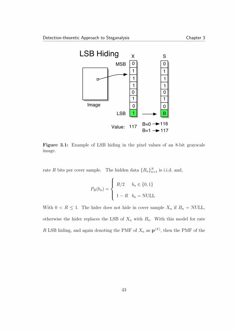
Detection-theoretic Approach to Steganalysis Chapter 3
1
B1Image
0
0
0
111
MSB
LSB
0
0
0
111
1
Value: 117117116B=0
B=1
X SLSB Hiding
Figure 3.1: Example of LSB hiding in the pixel values of an 8-bit grayscaleimage.
rate R bits per cover sample. The hidden data {Bn}Nn=1 is i.i.d. and,
PB(bn) =
R/2 bn ∈ {0, 1}
1−R bn = NULL
With 0 < R ≤ 1. The hider does not hide in cover sample Xn if Bn = NULL,
otherwise the hider replaces the LSB of Xn with Bn. With this model for rate
R LSB hiding, and again denoting the PMF of Xn as p(X), then the PMF of the
43
Detection-theoretic Approach to Steganalysis Chapter 3
stego data after LSB hiding at rate R is given by,
p(SR)i =
(1− R
2
)p
(X)i + R
2p
(X)i+1 i even
R2p
(X)i−1 +
(1− R
2
)p
(X)i i odd
For a more concise notation, we can write p(SR) = QRp(X), where QR is a 256×256
matrix corresponding to the above linear transformation.
3.2.2 Optimal Composite Hypothesis Testing for LSB Ste-
ganalysis
Since LSB hiding can embed a particularly high volume of data, the stega-
nographer may purposely hide less in order to evade detection; hence we must
account for the hiding rate. In this section, for the i.i.d. cover and LSB hiding
described above, we extend the hypothesis testing model of Section 3.1 to a com-
posite hypothesis testing problem in which the hiding rate is not known. As with
other hiding schemes we consider, we first assume that the cover PMF is known
to the detector so as to characterize the optimal performance.
Rather than a simple test deciding between cover and stego, we wish to decide
between two possibilities: data is hidden at some rate R, where R0 ≤ R ≤ R1,
or no data is hidden (R = 0). The parameters 0 < R0 ≤ R1 ≤ 1 are specified
by the user. We use HR to represent the hypothesis that data is hidden at rate
44
Detection-theoretic Approach to Steganalysis Chapter 3
R. The steganalysis problem in this notation is to distinguish between H0 and
K(R0, R1) , {HR : R0 ≤ R ≤ R1}. The hypothesis that data is hidden is thus
composite while the hypothesis that nothing is hidden is simple. For this case our
detector is:
δ(Y1, ..., YN) =
H0 if (Y1, ..., YN) ∈ A,
K(R0, R1) if (Y1, ..., YN) ∈ Ac.
In [21], Dabeer proves for low-rate hiding that the optimal composite hypoth-
esis is solved by the simple hypothesis testing problem: test H0 versus HR0 . This
greatly simplifies the problem, allowing us to use the likelihood ratio test (or
minimum K-L divergence) introduced in Section 3.1.
3.2.3 Asymptotic Performance of Hypothesis Tests
Without having to simulate actual likelihood tests, we can estimate the per-
formance of detection from the K-L divergence. For the case of small divergence,
when the hiding introduces little change to the cover statistics, we can employ an
asymptotic normality assumption to the decision statistic, L(y). From this we
can calculate approximate expressions of the error probabilities for lage N and
different R. This allows us to avoid time-consuming Monte Carlo simulations
when evaluating detection, especially helpful when comparing between detection
methods.
45
Detection-theoretic Approach to Steganalysis Chapter 3
We note the empirical PMF of received data can be written as:
q =1
N
N∑n=1
Zn
where Zn is a column vector whose m-th entry is 1 if received data Yn = m and
is zero otherwise. As Yn are i.i.d., Zn are i.i.d., and we have then a sum of i.i.d.
random variables. From the central limit theorem, q converges in distribution to
the Gaussian:
q =⇒ N (E[Z1], N−1ΣR)
where ΣR is the covariance matrix of Z1. Under hypothesis HR, E[Z1] = p(SR),
and ΣR = diag(p(SR))− p(SR)(p(SR))T (for H0, we note that p(S0) ≡ p(X)). Now
suppose our decision processing statistic, L, is differentiable at p(SR), then [71]
L(q) =⇒ N (µ(R), N−1σ2(R))
µ(R) = L(p(SR))
σ2(R) = uTRΣRuR
uR , ∇L|p(SR) .
We are interested in finding expressions for the probabilities of errors for the
detector based on L(q). For LSB hiding, we are most concerned with small R,
around 0.05. Here the alternative hypotheses are close, and the asymptotic nor-
mality result provides good approximations to the error probabilities. For the
46
Detection-theoretic Approach to Steganalysis Chapter 3
large divergence case, in which the error region is several standard deviations
from the means, the central limit theorem becomes increasingly inaccurate. Here
we can use results from large deviation theory [22] to bound the error probabili-
ties. For example, a commonly used result in hypothesis testing is the Chernoff
bound [67], which we use in Section 3.3 for QIM detection. With the Gaussian
approximation for large N and small R we have
P (False Alarm) = P (L(q) < τ |H0)
≈ Q
(√N(µ(0)− τ)
σ(0)
)(3.3)
P (Miss) = P (L(q) ≥ τ |HR)
≈ Q
(√N(τ − µ(R))
σ(R)
)(3.4)
where Q() is the complementary Gaussian function:
Q(u) ,∫ ∞
u
1√2π
e−u2/2du
We now compare the LLRT to the χ2 (chi-squared) steganalysis test used by
Westfeld et al [100] and by Provos’ Stegdetect [69]. The decision statistic is
Lχ2(q) ,127∑k=0
(q2k+1 − q2k)2
q2k + q2k+1
.
47
Detection-theoretic Approach to Steganalysis Chapter 3
If Lχ2(q) is less than a threshold, then data is declared to be hidden, otherwise
the image is considered clean. We know that after hiding at R = 1,
p(SR)2k = p
(SR)2k+1 =
p(SR)2k + p
(SR)2k+1
2, 0 ≤ k ≤ 127
The χ2 statistic is a measure of the closeness of the adjacent bins {2k, 2k +
1}; A smaller statistic implies adjacent bin values are nearly equal, and there
is a high chance that data is hidden. To compare the two decision statistics,
the LLRT, L(q), and χ2, Lχ2(q), we use binomial cover PMFs, B{255, θ}, θ ∈
(0, 1) and mixtures of binomials. We observed that χ2 performs very close to the
optimal LLRT. While the χ2 statistic does not depend on the cover PMF and for
a given cover PMF its performance appears to be close to the LLRT, the choice of
threshold required to guarantee a target performance depends on the host PMF
as shown by the following example. Suppose our target is to minimize the error
sum P (Miss)+P (False Alarm). In Figure 3.2, we plot this error sum as a function
of the threshold for the LLRT and χ2 for binomial B{255,0.5} and B{255,0.8}
cover PMFs. For the LLRT, the threshold τ = 0 minimizes the error sum for any
cover PMF, whereas for χ2 the minimizing threshold depends on the cover PMF.
To summarize, if the cover PMF is known, then there is little loss in using
the suboptimal χ2 test. In practice this means that if we have good models for
the cover PMF and lookup tables for choosing the threshold (depending on the
cover PMF), the χ2 performs close to the LLRT. However, the cover PMF usually
48
Detection-theoretic Approach to Steganalysis Chapter 3
varies substantially over image databases, and hence we are more interested in
completely data driven test that attain the target performance; both the statistic
and the threshold have to be chosen based on the data to achieve the desired
performance. With this in mind, we note two points, which motivate our work in
the following section.
1. The likelihood ratio depends on the cover PMF. However the threshold τ
can be chosen independent of the cover PMF. For example to minimize the
error sum P (Miss) + P (False Alarm), we can choose τ = 0.
2. The χ2 statistic does not depend on the cover PMF, but to obtain a target
performance, the threshold τ has to be chosen depending on the cover PMF.
Thus χ2 does not resolve the problem of not knowing the cover PMF; it
simply transfers it to the choice of τ .
3.2.4 Practical Detection Based on LLRT
Given the discussion in Section 3.2.2, we now restrict our attention to the
simple hypothesis testing problem: test H0 versus HR, R > 0. We propose tests
based on the estimation of the LLRT statistic and exhibit their superiority over
χ2. We also develop estimates of the hiding rate R.
49
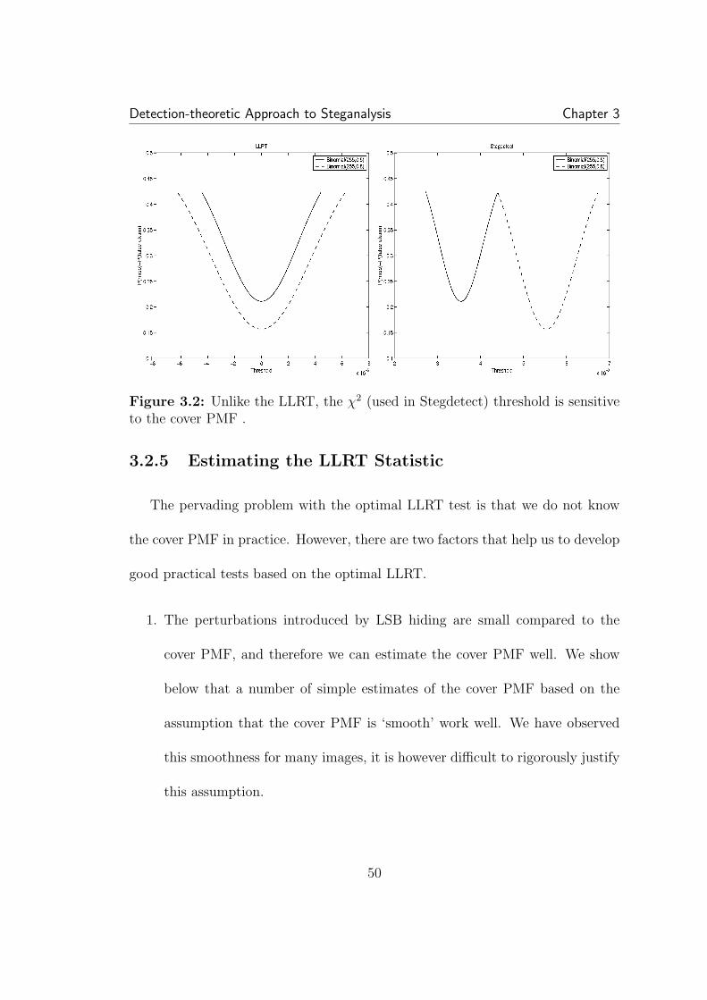
Detection-theoretic Approach to Steganalysis Chapter 3
Figure 3.2: Unlike the LLRT, the χ2 (used in Stegdetect) threshold is sensitiveto the cover PMF .
3.2.5 Estimating the LLRT Statistic
The pervading problem with the optimal LLRT test is that we do not know
the cover PMF in practice. However, there are two factors that help us to develop
good practical tests based on the optimal LLRT.
1. The perturbations introduced by LSB hiding are small compared to the
cover PMF, and therefore we can estimate the cover PMF well. We show
below that a number of simple estimates of the cover PMF based on the
assumption that the cover PMF is ‘smooth’ work well. We have observed
this smoothness for many images, it is however difficult to rigorously justify
this assumption.
50
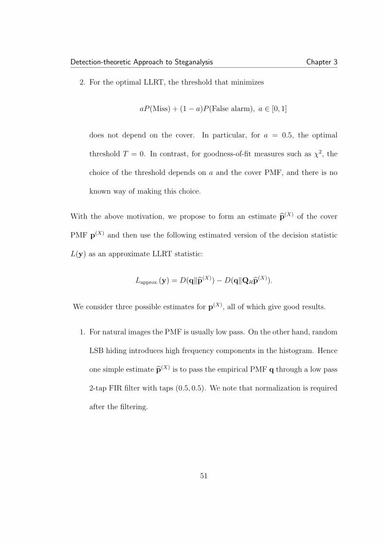
Detection-theoretic Approach to Steganalysis Chapter 3
2. For the optimal LLRT, the threshold that minimizes
aP (Miss) + (1− a)P (False alarm), a ∈ [0, 1]
does not depend on the cover. In particular, for a = 0.5, the optimal
threshold T = 0. In contrast, for goodness-of-fit measures such as χ2, the
choice of the threshold depends on a and the cover PMF, and there is no
known way of making this choice.
With the above motivation, we propose to form an estimate p(X) of the cover
PMF p(X) and then use the following estimated version of the decision statistic
L(y) as an approximate LLRT statistic:
Lapprox.(y) = D(q‖p(X))−D(q‖QRp(X)).
We consider three possible estimates for p(X), all of which give good results.
1. For natural images the PMF is usually low pass. On the other hand, random
LSB hiding introduces high frequency components in the histogram. Hence
one simple estimate p(X) is to pass the empirical PMF q through a low pass
2-tap FIR filter with taps (0.5, 0.5). We note that normalization is required
after the filtering.
51

Detection-theoretic Approach to Steganalysis Chapter 3
2. Another regularity constraint that we can impose on the cover PMF is that
local slope is preserved. That is,
p(X)k+3 − p
(X)k = 3(p
(X)k+2 − p
(X)k+1), k = 0, 4, 8, ..., 252.
This can be concisely written as Ap(X) = 0, where A is a 64× 256 matrix
corresponding to the regularity constraint. Under this constraint, a natural
estimate of p(X) is to project q on to the null space of A. We again need
normalization and removal of negative components after this filtering.
3. We also propose a non-linear approach that adapts to the underlying cover
PMF. We note that LSB hiding only affects the 8th bit plane. Therefore,
we impose the regularity constraint that the cover PMF is such that we
can obtain the cover PMF by spline interpolation of the first seven bit
planes. The corresponding estimate p(X) is obtained by subsampling q,
then interpolating using splines, and then normalizing.
We refer to all these tests as the approximate LLRT.
Simulation Results
In this section we report and discuss a number of simulation results for four
thousand images from a DOQQ image set, as well as digital camera and scanned
images.
52
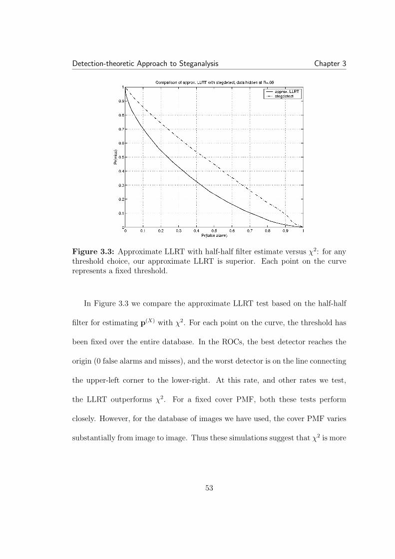
Detection-theoretic Approach to Steganalysis Chapter 3
Figure 3.3: Approximate LLRT with half-half filter estimate versus χ2: for anythreshold choice, our approximate LLRT is superior. Each point on the curverepresents a fixed threshold.
In Figure 3.3 we compare the approximate LLRT test based on the half-half
filter for estimating p(X) with χ2. For each point on the curve, the threshold has
been fixed over the entire database. In the ROCs, the best detector reaches the
origin (0 false alarms and misses), and the worst detector is on the line connecting
the upper-left corner to the lower-right. At this rate, and other rates we test,
the LLRT outperforms χ2. For a fixed cover PMF, both these tests perform
closely. However, for the database of images we have used, the cover PMF varies
substantially from image to image. Thus these simulations suggest that χ2 is more
53
Detection-theoretic Approach to Steganalysis Chapter 3
sensitive to the choice of the threshold than our approximate LLRT test. This is
not surprising since we know that to attain a target performance, the choice of the
threshold in LLRT does not depend on the cover PMF. For example, if we choose
T = 0 for the approximate LLRT in the case when the hiding rate is 0.05, then we
found the operating point to be P (Miss) = 0.4043 and P (False Alarm) = 0.3219.
From Figure 3.3 we can verify that the tangent to the operating curve at this
point is of slope approximately 1 as predicted by the theory. The approximate
LLRT is therefore closer to the goal of finding a data driven test.
Figure 3.4: Hiding in the LSBs of JPEG coefficients: again LRT based methodis superior to χ2.
54
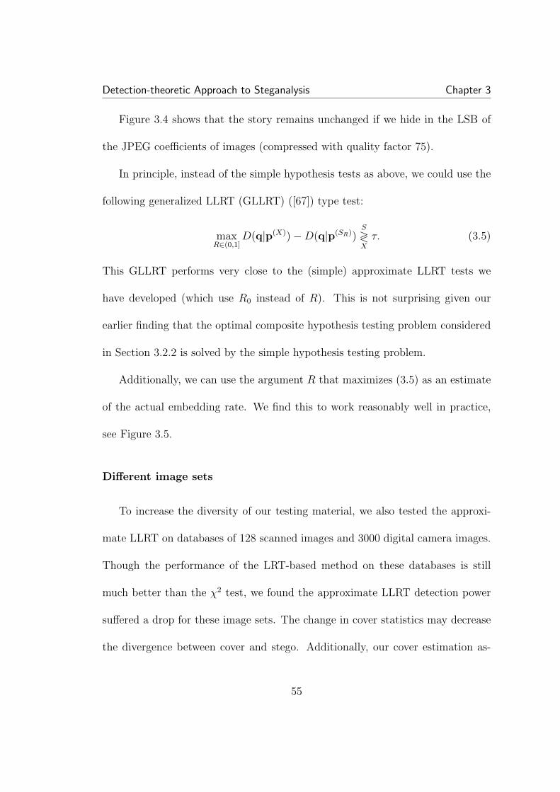
Detection-theoretic Approach to Steganalysis Chapter 3
Figure 3.4 shows that the story remains unchanged if we hide in the LSB of
the JPEG coefficients of images (compressed with quality factor 75).
In principle, instead of the simple hypothesis tests as above, we could use the
following generalized LLRT (GLLRT) ([67]) type test:
maxR∈(0,1]
D(q|p(X))−D(q|p(SR))S
≷X
τ. (3.5)
This GLLRT performs very close to the (simple) approximate LLRT tests we
have developed (which use R0 instead of R). This is not surprising given our
earlier finding that the optimal composite hypothesis testing problem considered
in Section 3.2.2 is solved by the simple hypothesis testing problem.
Additionally, we can use the argument R that maximizes (3.5) as an estimate
of the actual embedding rate. We find this to work reasonably well in practice,
see Figure 3.5.
Different image sets
To increase the diversity of our testing material, we also tested the approxi-
mate LLRT on databases of 128 scanned images and 3000 digital camera images.
Though the performance of the LRT-based method on these databases is still
much better than the χ2 test, we found the approximate LLRT detection power
suffered a drop for these image sets. The change in cover statistics may decrease
the divergence between cover and stego. Additionally, our cover estimation as-
55
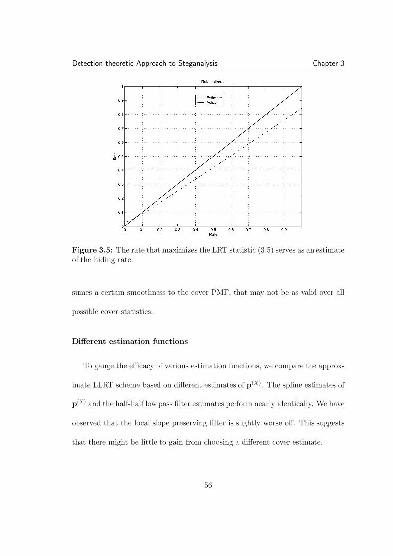
Detection-theoretic Approach to Steganalysis Chapter 3
Figure 3.5: The rate that maximizes the LRT statistic (3.5) serves as an estimateof the hiding rate.
sumes a certain smoothness to the cover PMF, that may not be as valid over all
possible cover statistics.
Different estimation functions
To gauge the efficacy of various estimation functions, we compare the approx-
imate LLRT scheme based on different estimates of p(X). The spline estimates of
p(X) and the half-half low pass filter estimates perform nearly identically. We have
observed that the local slope preserving filter is slightly worse off. This suggests
that there might be little to gain from choosing a different cover estimate.
56
Detection-theoretic Approach to Steganalysis Chapter 3
Comparison with RS
The focus to this point has been to develop the optimal methodology for
steganalysis of i.i.d. data. RS analysis [33] is a non-hypothesis testing based algo-
rithm for estimating the length of an LSB hidden message that exploits correla-
tion. By comparing with our approximate LLRT we can gauge the improvement
that can be gained by including cover memory. In Figure 3.6, we can see the im-
provement gained by acknowledging the cover correlation. Other image databases
showed similar gains. In Chapter 4 we extend the detection theoretic framework
to include a notion of cover memory.
S-tools
We further test our approximate LLRT LSB detection on S-Tools [9], a popular
software for data hiding that uses an LSB hiding method. One function of S-
tools is to hide data into color images. Though we generally focus on grayscale
images, we test our detection on S-tools because it is a freely available and popular
tool. We embedded random data at maximum rate using S-tools in a database
of hundreds of color images. This database is comprised of images from two
sources: images from a Corel photo CD and images scanned from photographs.
The Corel photos had to be converted from PCD format to BMP for embedding,
and the scanned images are converted from PNG format. The approximate LLRT
57
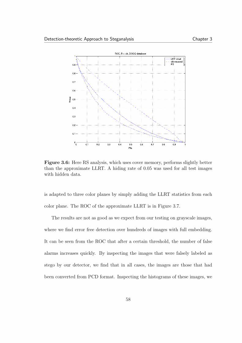
Detection-theoretic Approach to Steganalysis Chapter 3
Figure 3.6: Here RS analysis, which uses cover memory, performs slightly betterthan the approximate LLRT. A hiding rate of 0.05 was used for all test imageswith hidden data.
is adapted to three color planes by simply adding the LLRT statistics from each
color plane. The ROC of the approximate LLRT is in Figure 3.7.
The results are not as good as we expect from our testing on grayscale images,
where we find error free detection over hundreds of images with full embedding.
It can be seen from the ROC that after a certain threshold, the number of false
alarms increases quickly. By inspecting the images that were falsely labeled as
stego by our detector, we find that in all cases, the images are those that had
been converted from PCD format. Inspecting the histograms of these images, we
58
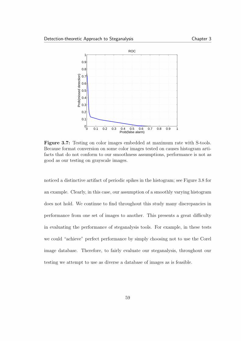
Detection-theoretic Approach to Steganalysis Chapter 3
0 0.1 0.2 0.3 0.4 0.5 0.6 0.7 0.8 0.9 10
0.1
0.2
0.3
0.4
0.5
0.6
0.7
0.8
0.9
1ROC
Prob(false alarm)
Pro
b(m
isse
d de
tect
ion)
Figure 3.7: Testing on color images embedded at maximum rate with S-tools.Because format conversion on some color images tested on causes histogram arti-facts that do not conform to our smoothness assumptions, performance is not asgood as our testing on grayscale images.
noticed a distinctive artifact of periodic spikes in the histogram; see Figure 3.8 for
an example. Clearly, in this case, our assumption of a smoothly varying histogram
does not hold. We continue to find throughout this study many discrepancies in
performance from one set of images to another. This presents a great difficulty
in evaluating the performance of steganalysis tools. For example, in these tests
we could “achieve” perfect performance by simply choosing not to use the Corel
image database. Therefore, to fairly evaluate our steganalysis, throughout our
testing we attempt to use as diverse a database of images as is feasible.
59
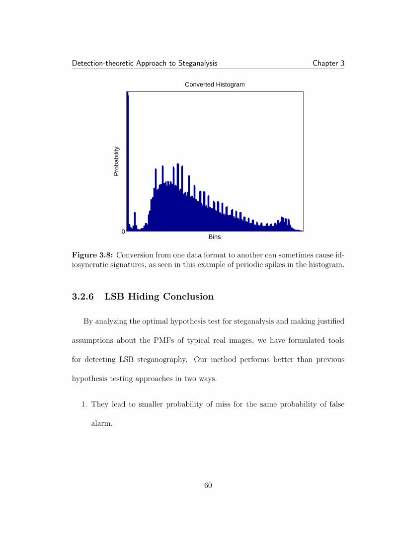
Detection-theoretic Approach to Steganalysis Chapter 3
0Bins
Pro
babi
lity
Converted Histogram
Figure 3.8: Conversion from one data format to another can sometimes cause id-iosyncratic signatures, as seen in this example of periodic spikes in the histogram.
3.2.6 LSB Hiding Conclusion
By analyzing the optimal hypothesis test for steganalysis and making justified
assumptions about the PMFs of typical real images, we have formulated tools
for detecting LSB steganography. Our method performs better than previous
hypothesis testing approaches in two ways.
1. They lead to smaller probability of miss for the same probability of false
alarm.
60

Detection-theoretic Approach to Steganalysis Chapter 3
2. The choice of the threshold is less sensitive to variations in the cover PMF.
Thus for typical hiding rates less than 0.1, the choice of threshold τ = 0
leads to good performance.
61
Detection-theoretic Approach to Steganalysis Chapter 3
3.3 Quantization Index Modulation Hiding
Quantization index modulation (QIM) [14] is another popular hiding method.
Though more complex and generally with lower capacity than LSB hiding, QIM
is much more robust to noise and attacks. The essential idea of quantization
based data hiding is to quantize the cover signal with a quantizer indexed by the
message. Again, denote the cover and stego signals as {Xn}Nn=1 and {Sn}N
n=1,
and let b be the message. We have S(X, b) = qb(X). The stego signal consists
only of values in the set of quantizer outputs. This is appropriate if the signal is
expected to be quantized, for compression for example. Dither modulation [14],
can produce a stego signal covering all of the values of the cover signal. Here the
quantizers are shifted according to a changing dither level D
S(X,m) = qb(X + D)−D = q(X + D(b))−D(b) (3.6)
There exist more advanced flavors of QIM, which provide advantages to simpler
versions, but these are generally designed for watermarking applications. For
example, we note that while distortion compensated QIM (DC-QIM) has perfor-
mance benefits for watermarking, the statistical effect of DC-QIM is so distinctive
[98] that we believe it is not suitable for covert data hiding. Most practical im-
plementations we have seen use either simple QIM, or dither modulation, with
uniform scalar quantizers, thus we focus on these.
62
Detection-theoretic Approach to Steganalysis Chapter 3
We note also that typically a steganographer is hiding in data transformed to
make it suitable for compression. This is done for two reasons. First, hiding in
a compression transform spreads the hidden data over a large region, making it
less susceptible to local attacks. Second, the image is likely compressed if it is
transmitted, and hiding in the compressed medium allows the steganographer to
more easily anticipate the effect of compression. (For a thorough exploration of
the validity of these assumptions see [102].)
3.3.1 Statistical Model for QIM Hiding
To apply our detection-theoretic approach, we need a description of the effect
of uniform scalar QIM hiding on the cover PMF. For uniform scalar QIM, one
bit, b, of the message is embedded into each sample. The quantizer function qb is
qb(X) =
round(X/∆) b = 0
round(X/∆) + ∆/2 b = 1
see Figure 3.9.
For the steganographer, the choice of ∆ represents a trade off between ro-
bustness and distortion to the image. Later we show ∆’s relationship to the
steganographic security. The relationship of ∆ to robustness depends on what
we define as robust. For robustness to the classical additive white Gaussian noise
63
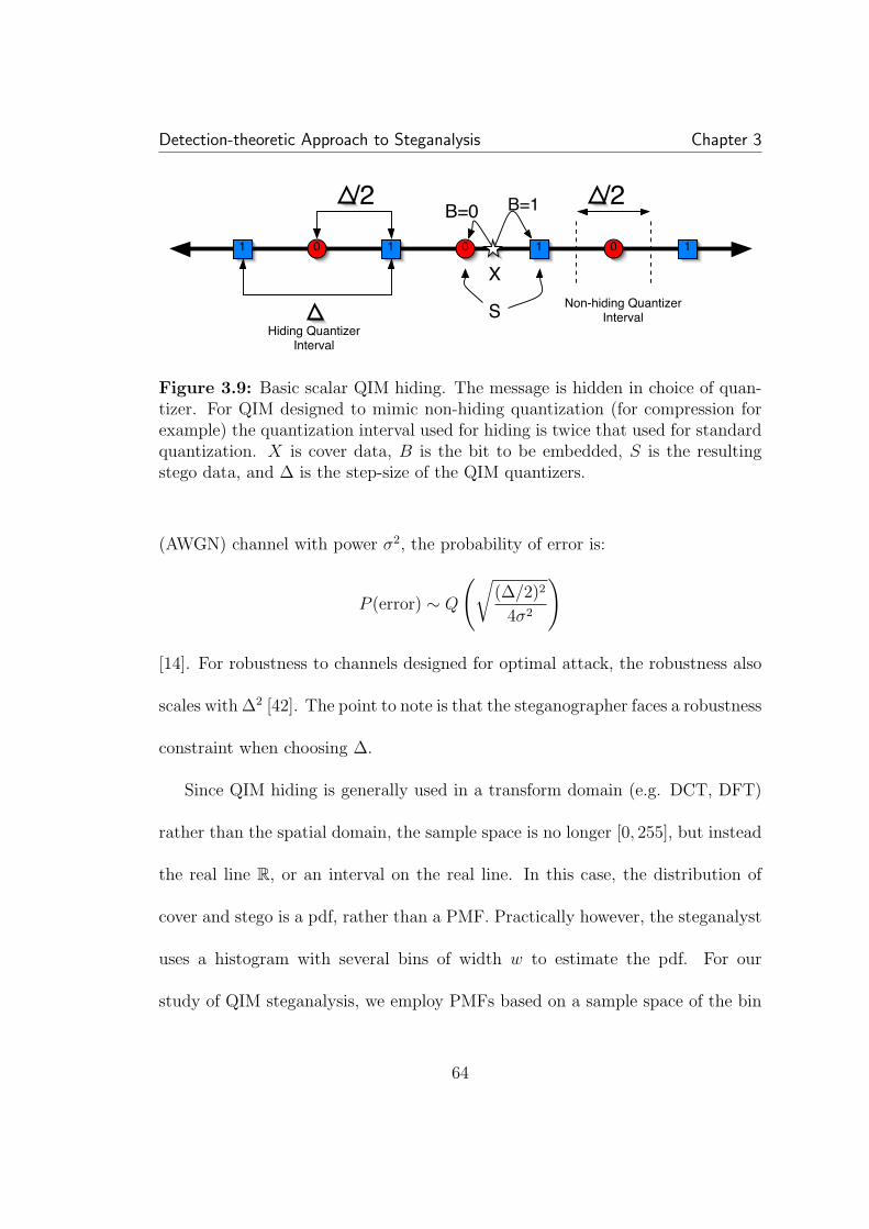
Detection-theoretic Approach to Steganalysis Chapter 3
1 0 0 01 1
X
B=0 B=1/2
S
1
Non-hiding QuantizerInterval
/2
Hiding QuantizerInterval
Figure 3.9: Basic scalar QIM hiding. The message is hidden in choice of quan-tizer. For QIM designed to mimic non-hiding quantization (for compression forexample) the quantization interval used for hiding is twice that used for standardquantization. X is cover data, B is the bit to be embedded, S is the resultingstego data, and ∆ is the step-size of the QIM quantizers.
(AWGN) channel with power σ2, the probability of error is:
P (error) ∼ Q
(√(∆/2)2
4σ2
)
[14]. For robustness to channels designed for optimal attack, the robustness also
scales with ∆2 [42]. The point to note is that the steganographer faces a robustness
constraint when choosing ∆.
Since QIM hiding is generally used in a transform domain (e.g. DCT, DFT)
rather than the spatial domain, the sample space is no longer [0, 255], but instead
the real line R, or an interval on the real line. In this case, the distribution of
cover and stego is a pdf, rather than a PMF. Practically however, the steganalyst
uses a histogram with several bins of width w to estimate the pdf. For our
study of QIM steganalysis, we employ PMFs based on a sample space of the bin
64
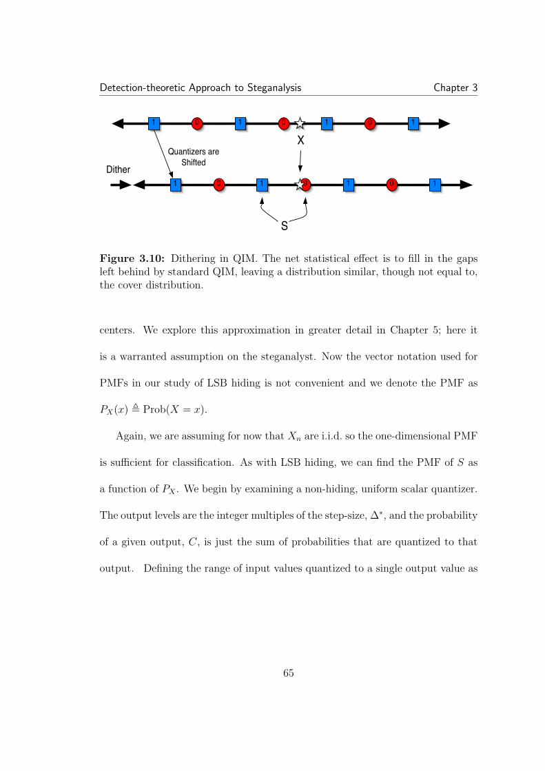
Detection-theoretic Approach to Steganalysis Chapter 3
1 0 0 01 1
X1
1 0 0 01 1
S
1Dither
Quantizers areShifted
Figure 3.10: Dithering in QIM. The net statistical effect is to fill in the gapsleft behind by standard QIM, leaving a distribution similar, though not equal to,the cover distribution.
centers. We explore this approximation in greater detail in Chapter 5; here it
is a warranted assumption on the steganalyst. Now the vector notation used for
PMFs in our study of LSB hiding is not convenient and we denote the PMF as
PX(x) , Prob(X = x).
Again, we are assuming for now that Xn are i.i.d. so the one-dimensional PMF
is sufficient for classification. As with LSB hiding, we can find the PMF of S as
a function of PX . We begin by examining a non-hiding, uniform scalar quantizer.
The output levels are the integer multiples of the step-size, ∆∗, and the probability
of a given output, C, is just the sum of probabilities that are quantized to that
output. Defining the range of input values quantized to a single output value as
65
Detection-theoretic Approach to Steganalysis Chapter 3
X ∗(c) , [c−∆∗/2, c + ∆∗/2) then the PMF is
PC(c) =
∑
x∈X ∗(c) PX(x), c ∈ k∆∗
0 else
(3.7)
Where k is any integer. If now the choice of quantizer is used to hide binary data,
B, we split the original quantizer into two coarser subsets, each with step-size
∆ = 2∆∗. The quantizer associated with sending a 1 is identical to that as for
sending 0, but shifted by ∆/2. Assuming the probability of 0 is equal to 1, we
have
PS(s) =
12
∑x∈X (s) PX(x) s ∈ k∆
2
0 else
(3.8)
Where X (s) , [s−∆/2, s + ∆/2) is the analogous range for the new ∆. Unlike
standard quantization, these regions overlap for adjacent values of s. We note at
this point that if the goal of the steganographer is to mimic an existing quantizer,
for example a compression scheme, then the hider can stop here, without using
dither modulation. In [81] and [54], the authors use this to imitate the output
of JPEG and JPEG2000 respectively. We examine the detection of this first case
below.
For dither modulation, we let D be a pseudorandom (PR) variable uniformly
distributed over [−∆/4, ∆/4) so that the output covers all the values of the input,
and does not leave tell-tale signs of quantization. Under our PMF approximation,
66
Detection-theoretic Approach to Steganalysis Chapter 3
PD(d) = 2w/∆. With this dithering, any S is valid. For every received value of
S there is one and only one valid value of D and one valid value of B that could
have made that s. For any valid S, PS(s) = PB(required b) ∩∑
x∈X (s) PX(x) ∩
PD(required d). Assuming equiprobable message data P (b) is 12
for either 0 or
1. Similarly since PD is uniform, the probability is the same for any d so after
plugging in we have
PS(s) =w
∆
∑x∈X (s)
PX(x) (3.9)
We note D can alternatively be distributed over [−∆/2, ∆/2) with no change on
the distribution of S [98]. Additionally in this case it has been shown that S and
X are statistically independent [40].
3.3.2 Optimal Detection Performance
Armed with equations (3.7), (3.8), and (3.9) we can find the performance of
a detector operating in two scenarios. The first is distinguishing between cover
values that have been quantized versus QIM data embedding (without dithering).
The second case is distinguishing between an unquantized cover and a cover with
dithered QIM data embedded.
As mentioned in Section 3.1, the optimal detector is the log-likelihood ratio
test. Before we analyze the performance of this detector for some example PMFs,
67
Detection-theoretic Approach to Steganalysis Chapter 3
we can gain some insight into what is detectable simply by inspecting the log-
likelihood ratio (3.1):
Case I Quantized cover versus non-dithered QIM hiding:
Here we compare to A rather than X. The yk in y are independent, so L(y)
is:
L(y) = logN∏
i=1
1/2∑
yk−∆/2≤x<yk+∆/2 PX(x)∑yk−∆/4≤x<yk+∆/4 PX(x)
Basically hiding sums over twice the range, and compensates by halving the
total. Therefore a smoothly varying PMF is more difficult to detect than a
spikey one.
Case II Non-quantized cover versus dither modulation hiding:
L(y) = logN∏
k=1
(w/∆)∑
yk−∆/2≤x<yk+∆/2 PX(x)
PX(yk)
The product terms are exactly the ratio of the average (over ∆) to the
original. Dither modulation hiding therefore acts as a moving average filter
on the PMF. Alternatively it is the convolution of a uniform PMF with
twice the range of the dither sequence, and is therefore similar to SS hiding.
Intuitively, cover PMFs with high frequency components relative to ∆ are
much easier to detect than a smoothly varying PMF. Indeed, as is noted in
[43], a uniformly distributed cover would be impossible to detect.
68
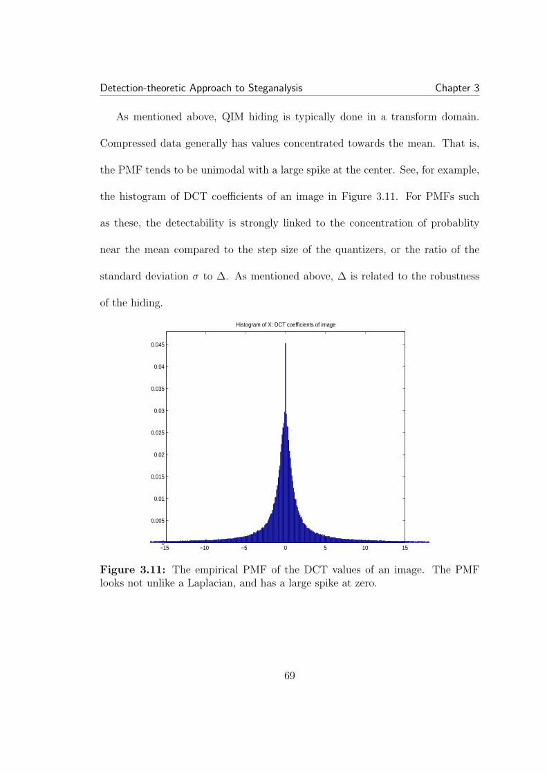
Detection-theoretic Approach to Steganalysis Chapter 3
As mentioned above, QIM hiding is typically done in a transform domain.
Compressed data generally has values concentrated towards the mean. That is,
the PMF tends to be unimodal with a large spike at the center. See, for example,
the histogram of DCT coefficients of an image in Figure 3.11. For PMFs such
as these, the detectability is strongly linked to the concentration of probablity
near the mean compared to the step size of the quantizers, or the ratio of the
standard deviation σ to ∆. As mentioned above, ∆ is related to the robustness
of the hiding.
−15 −10 −5 0 5 10 150
0.005
0.01
0.015
0.02
0.025
0.03
0.035
0.04
0.045
Histogram of X: DCT coefficients of image
Figure 3.11: The empirical PMF of the DCT values of an image. The PMFlooks not unlike a Laplacian, and has a large spike at zero.
69
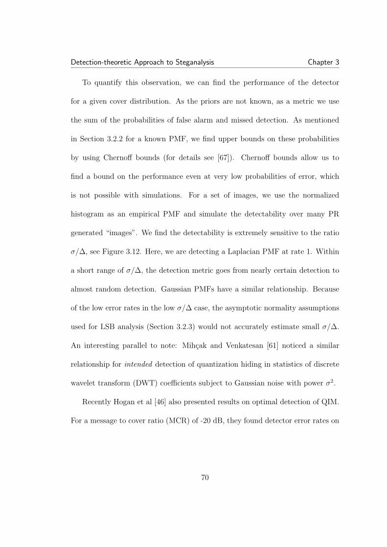
Detection-theoretic Approach to Steganalysis Chapter 3
To quantify this observation, we can find the performance of the detector
for a given cover distribution. As the priors are not known, as a metric we use
the sum of the probabilities of false alarm and missed detection. As mentioned
in Section 3.2.2 for a known PMF, we find upper bounds on these probabilities
by using Chernoff bounds (for details see [67]). Chernoff bounds allow us to
find a bound on the performance even at very low probabilities of error, which
is not possible with simulations. For a set of images, we use the normalized
histogram as an empirical PMF and simulate the detectability over many PR
generated “images”. We find the detectability is extremely sensitive to the ratio
σ/∆, see Figure 3.12. Here, we are detecting a Laplacian PMF at rate 1. Within
a short range of σ/∆, the detection metric goes from nearly certain detection to
almost random detection. Gaussian PMFs have a similar relationship. Because
of the low error rates in the low σ/∆ case, the asymptotic normality assumptions
used for LSB analysis (Section 3.2.3) would not accurately estimate small σ/∆.
An interesting parallel to note: Mihcak and Venkatesan [61] noticed a similar
relationship for intended detection of quantization hiding in statistics of discrete
wavelet transform (DWT) coefficients subject to Gaussian noise with power σ2.
Recently Hogan et al [46] also presented results on optimal detection of QIM.
For a message to cover ratio (MCR) of -20 dB, they found detector error rates on
70
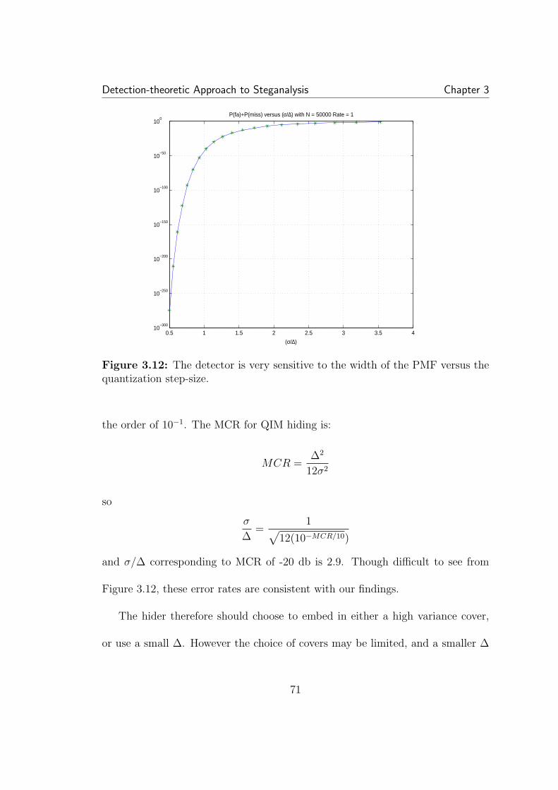
Detection-theoretic Approach to Steganalysis Chapter 3
0.5 1 1.5 2 2.5 3 3.5 410
−300
10−250
10−200
10−150
10−100
10−50
100
P(fa)+P(miss) versus (σ/∆) with N = 50000 Rate = 1
(σ/∆)
P(f
a)+
P(m
iss)
Figure 3.12: The detector is very sensitive to the width of the PMF versus thequantization step-size.
the order of 10−1. The MCR for QIM hiding is:
MCR =∆2
12σ2
so
σ
∆=
1√12(10−MCR/10)
and σ/∆ corresponding to MCR of -20 db is 2.9. Though difficult to see from
Figure 3.12, these error rates are consistent with our findings.
The hider therefore should choose to embed in either a high variance cover,
or use a small ∆. However the choice of covers may be limited, and a smaller ∆
71
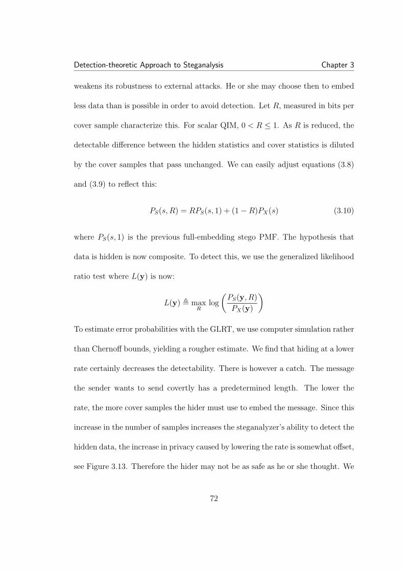
Detection-theoretic Approach to Steganalysis Chapter 3
weakens its robustness to external attacks. He or she may choose then to embed
less data than is possible in order to avoid detection. Let R, measured in bits per
cover sample characterize this. For scalar QIM, 0 < R ≤ 1. As R is reduced, the
detectable difference between the hidden statistics and cover statistics is diluted
by the cover samples that pass unchanged. We can easily adjust equations (3.8)
and (3.9) to reflect this:
PS(s, R) = RPS(s, 1) + (1−R)PX(s) (3.10)
where PS(s, 1) is the previous full-embedding stego PMF. The hypothesis that
data is hidden is now composite. To detect this, we use the generalized likelihood
ratio test where L(y) is now:
L(y) , maxR
log
(PS(y, R)
PX(y)
)
To estimate error probabilities with the GLRT, we use computer simulation rather
than Chernoff bounds, yielding a rougher estimate. We find that hiding at a lower
rate certainly decreases the detectability. There is however a catch. The message
the sender wants to send covertly has a predetermined length. The lower the
rate, the more cover samples the hider must use to embed the message. Since this
increase in the number of samples increases the steganalyzer’s ability to detect the
hidden data, the increase in privacy caused by lowering the rate is somewhat offset,
see Figure 3.13. Therefore the hider may not be as safe as he or she thought. We
72
Detection-theoretic Approach to Steganalysis Chapter 3
illustrate this with an example. Suppose a hider is sending a 15,000 bit message
in 50,000 cover samples (R = 0.3). If the cover is a Gaussian with (σ/∆) = 1
the detector has an error sum (the probability of false alarm plus probability of
missed detection) of 0.070. If we hold the number of samples constant but halve
the rate to R = 0.15, the sum of errors jumps to 0.366, because of the reduction
in rate. However this only sends 7,500 bits. To send the entire message the hider
has to use 100,000 cover samples. The error sum for the steganalyst taking this
into account drops to 0.205.
103
104
105
106
107
10−300
10−250
10−200
10−150
10−100
10−50
100
P(fa)+P(miss) vs N for Rate = 1, (σ/∆) = 1
Number of samples
op
tima
l P(f
a)
+ P
(mis
s)
Figure 3.13: Detection error as a function of the number of samples. The coverPMF is a Gaussian with (σ/∆) = 1
73
Detection-theoretic Approach to Steganalysis Chapter 3
3.3.3 Practical Detection
Finally, in implementing these schemes on real world data, certain adjustments
must be made to the basic scheme. For example both [81] and [54] exclude low-
valued coefficients from embedding. This is done to avoid visual distortion of the
final image, and to prevent the characteristic smoothing of probability near the
mean we observed above. This thresholding however leaves a new characteristic
effect on the PMF near the low values. The derivation of this modified stego PMF
is straightforward but lengthy and offers little illumination.
We do not have access to the cover statistics in a practical detection setting.
To overcome this, we can attempt to estimate the cover statistics for each received
image, or estimate the cover statistics for all images. Some steganalysis is able
to estimate the statistics on an image by image basis, as in our work with LSB
hiding and the work by Fridrich et al on detecting F5 [35], however there is no
general prescription for making such an estimate. As noted in Chapter 2, there
has also been some success with classifying between the set of all cover images and
all stego images through the use of supervised learning techniques. The idea is to
train a machine with several examples of both cover and stego, and the machine
learns to discriminate between the two classes. For our experiments we choose to
employ supervised learning.
74
Detection-theoretic Approach to Steganalysis Chapter 3
Motivated by the likelihood ratio test, we use an empirical PMF (histogram)
as the feature vector. We performed simulated detection of a DCT-based QIM
scheme [81]. This scheme is designed to use the same quantization as JPEG. The
hiding is designed for a given JPEG quality factor, which translates to a set of
quantization step sizes for different DCT frequencies. Higher quality factor implies
smaller step size. Since the quality factor used is not known by the steganalyst, ∆
is not available. In an attempt to capture the variety of real-world images, we use
three databases: digital orthophoto quarter-quadrangle (DOQQ) aerial images
used also for testing LSB hiding, Corel PhotoCD (CPCD) images, and images
taken with a Canon digital camera (CACD), also used for LSB testing. For a
classifier we use Joachim’s support vector machine (SVM) implementation [51],
SVMlight. A linear kernel is used; we found other kernels perform only slightly
differently. We perform the following two tests:
With constant design quality factor: In the first experiment, we set the
design quality factor at 50 to hide data in images in both the training and testing
sets. Since the quality factor is static, ∆ is the same for all stego images, aiding
the classifier. After hiding, both the cover images and the images with hidden
content are compressed to JPEG at the same quality factor in order to avoid
detection of JPEG compression. The results of detection error for this test are
shown in Table 3.1 We find that if the design quality factor is constant, the
75
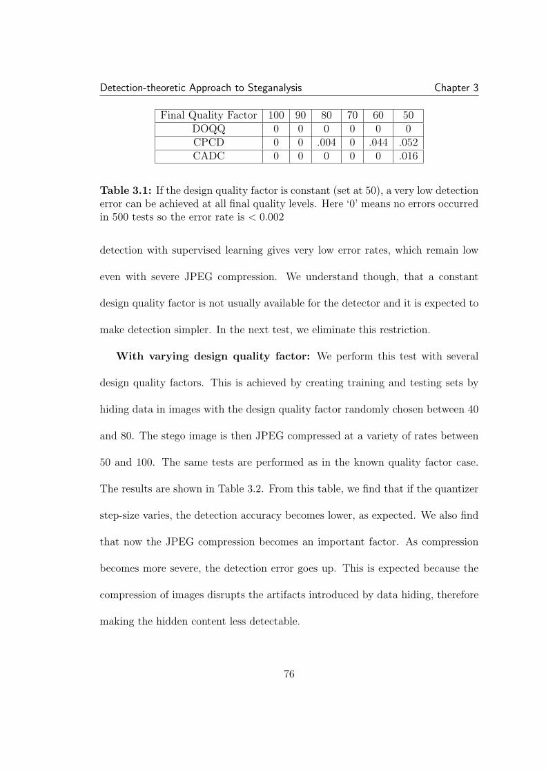
Detection-theoretic Approach to Steganalysis Chapter 3
Final Quality Factor 100 90 80 70 60 50DOQQ 0 0 0 0 0 0CPCD 0 0 .004 0 .044 .052CADC 0 0 0 0 0 .016
Table 3.1: If the design quality factor is constant (set at 50), a very low detectionerror can be achieved at all final quality levels. Here ‘0’ means no errors occurredin 500 tests so the error rate is < 0.002
detection with supervised learning gives very low error rates, which remain low
even with severe JPEG compression. We understand though, that a constant
design quality factor is not usually available for the detector and it is expected to
make detection simpler. In the next test, we eliminate this restriction.
With varying design quality factor: We perform this test with several
design quality factors. This is achieved by creating training and testing sets by
hiding data in images with the design quality factor randomly chosen between 40
and 80. The stego image is then JPEG compressed at a variety of rates between
50 and 100. The same tests are performed as in the known quality factor case.
The results are shown in Table 3.2. From this table, we find that if the quantizer
step-size varies, the detection accuracy becomes lower, as expected. We also find
that now the JPEG compression becomes an important factor. As compression
becomes more severe, the detection error goes up. This is expected because the
compression of images disrupts the artifacts introduced by data hiding, therefore
making the hidden content less detectable.
76
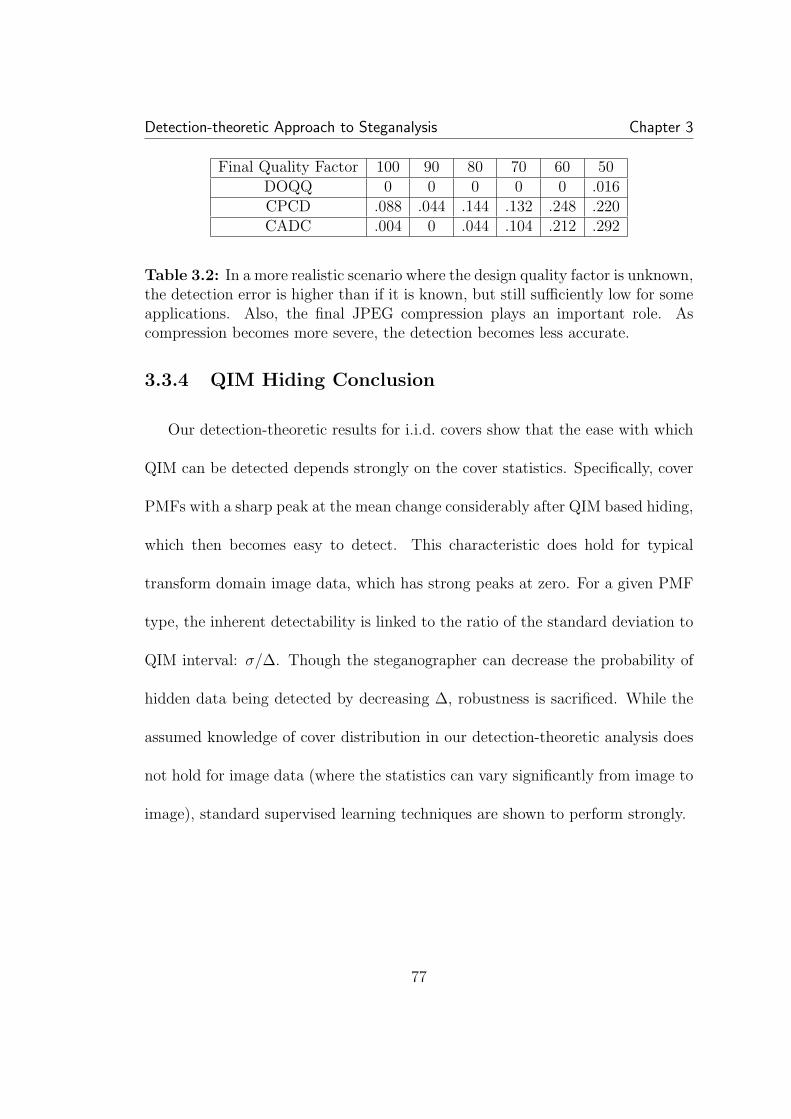
Detection-theoretic Approach to Steganalysis Chapter 3
Final Quality Factor 100 90 80 70 60 50DOQQ 0 0 0 0 0 .016CPCD .088 .044 .144 .132 .248 .220CADC .004 0 .044 .104 .212 .292
Table 3.2: In a more realistic scenario where the design quality factor is unknown,the detection error is higher than if it is known, but still sufficiently low for someapplications. Also, the final JPEG compression plays an important role. Ascompression becomes more severe, the detection becomes less accurate.
3.3.4 QIM Hiding Conclusion
Our detection-theoretic results for i.i.d. covers show that the ease with which
QIM can be detected depends strongly on the cover statistics. Specifically, cover
PMFs with a sharp peak at the mean change considerably after QIM based hiding,
which then becomes easy to detect. This characteristic does hold for typical
transform domain image data, which has strong peaks at zero. For a given PMF
type, the inherent detectability is linked to the ratio of the standard deviation to
QIM interval: σ/∆. Though the steganographer can decrease the probability of
hidden data being detected by decreasing ∆, robustness is sacrificed. While the
assumed knowledge of cover distribution in our detection-theoretic analysis does
not hold for image data (where the statistics can vary significantly from image to
image), standard supervised learning techniques are shown to perform strongly.
77

Detection-theoretic Approach to Steganalysis Chapter 3
3.4 Summary
In this chapter we introduced our detection-theoretic approach to steganal-
ysis, and applied it to the detection of LSB and QIM methods of data hiding.
We found both steganographic methods to be theoretically detectable and de-
signed practical schemes with which to detect hiding in real images. Our initial
approach to applying detection theory to steganalysis has been to use an i.i.d.
model. A natural extension to this is to use a model including at least one level
of dependency, an extension we consider in the following chapter.
78
Chapter 4
Extending Detection-theoreticSteganalysis to Include Memory
As noted in Chapter 2 there are several practical image steganalysis techniques
which exploit interpixel correlations in images. Additionally, our work in applying
detection theory with an i.i.d. model to detection of LSB and QIM has hinted
that extending our model to include a degree of dependency will improve our
estimates and methods. In this chapter we employ a Markov model with our
detection-theoretic approach.
4.1 Introduction
Existing theoretical benchmarks of optimal detection such as Cachins’s ε-
secure measure [10] model the cover data as i.i.d., and therefore underestimate
the attainable steganalysis performance. We now take the logical next step to-
79
Extending Detection-theoretic Steganalysis to Include Memory Chapter 4
wards computing a more accurate performance benchmark, modeling the cover
data as a Markov chain (MC). The Markov model has the advantage of analytical
tractability, in that performance benchmarks governing detection performance
can be characterized and computed explicitly. In our examples and numerical
results, we focus on images as cover data, using a Markov model in which sta-
tistical dependency is limited to an adjacent pixel. Clearly, this model does not
completely capture interpixel dependencies. However, we find that the perfor-
mance benchmarks we compute are consistent with the performance of a number
of image steganalysis techniques that exploit spatial correlations.
With the extension of analysis to include dependency, we see immediate bene-
fits over current i.i.d. analysis. For example, though spread spectrum (SS) hiding
can be detected with reasonable accuracy using current steganalysis techniques
[45, 11, 86], security tests derived from i.i.d. analysis determine that spread spec-
trum hiding is in fact safe from detection. Markov chain analysis, on the other
hand, correctly determines SS hiding to be at risk from steganalysis. Addition-
ally, though recently steganographic schemes have been designed to reduce the
probability of detection, the efforts have generally focused on matching the one-
dimensional histogram [68, 26, 75] or other specific steganalysis statistics [76, 29],
which provides no guarantee that a future steganalysis scheme will not be able
to detect the hiding by using a different statistic. Furthermore, though the γD-
80
Extending Detection-theoretic Steganalysis to Include Memory Chapter 4
security, proposed by Chandramouli et al [12], does not use an i.i.d. assumption,
the measure is with respect to a given detector, and does not gauge the per-
formance of other detectors. On the other hand our analysis predicts optimal
steganalysis based on a Markov chain assumption. Although the MC model does
not completely characterize image statistics, practical constraints on the ability
of the steganalyst to estimate more complex statistical models have limited and
may continue to limit the complexity of detectors.
4.2 Detection Theory and Statistically Depen-
dent Data
We here outline our steganalysis approach using a Markov chain model, and
show how it relates to common steganalysis techniques.
4.2.1 Detection-theoretic Divergence Measure for Markov
Chains
To include interpixel dependency in our analysis, we employ a Markov chain
(MC) [16] model of image data. A Markov chain is a random sequence indexed
by n, subject to the following condition: P (Yn|Yn−1, Yn−2, . . . , Y1) = P (Yn|Yn−1).
Under this model, the probability of a given pixel is dependent on an immediately
81
Extending Detection-theoretic Steganalysis to Include Memory Chapter 4
adjacent pixel. We have used this model to analyze and detect spread spectrum
hiding [86]. In independent work, Sidorov has performed MC and Markov ran-
dom field analysis on detecting LSB hiding [78]. There are a number of reasons
to use a MC model. First, the MC model accounts for dependency, yet is very
general and flexible. Second, while a MC model is more complex than an i.i.d.
model, it is the least complex model incorporating dependencies. Though many
have used Markov random fields [70] to model images accounting for a larger
neighborhood of dependency than one adjacent pixel, for the steganalyst there is
a practical drawback to increasing the levels of dependency. As the model com-
plexity increases, the number of samples required to make an accurate estimate of
the statistics also increases. However the number of received samples depends on
the image size, and can not be increased by the steganalyst. Thus although the
complexity for the steganalyst increases quickly, the benefit does not. For more
on the difficulties of multivariate density estimation see [96]. The MC model on
the other hand is simple enough to make realistic statistical estimates. This is
analogous to a nth order DPCM coding system, in which the benefit of an increase
in n, the number of pixels used for prediction, has been shown to quickly drop
after 2 or 3 [44]. Finally, a divergence metric which measures the performance of
optimal detection, analogous to the K-L divergence for i.i.d. sources, exists [64]
for Markov chains, which we examine below.
82
Extending Detection-theoretic Steganalysis to Include Memory Chapter 4
We first clarify our notation. Let {Yn}Nn=1 be a Markov chain on the finite
set Y . In our context Yn are the n-indexed set of pixels obtained by a row or
column scanning and Y are all possible gray scale values (e.g. for an 8-bit image,
Y = {0, 1, . . . , 255}). A Markov chain source is defined by a transition matrix,
Tij , P (Yn = i|Yn−1 = j), and marginal probabilities pi , P (Yn = i). For
a realization y = (y1, y2, . . . , yN)T , let ηij(y) be the number of transitions from
value i to value j in y. The empirical matrix is M(y) , (ηij(y)/(N − 1)). That
is, the i, j-th element represents the proportion of spatially adjacent pixel pairs
with a grayscale value of i followed by j, and therefore provides an estimate of the
probability P (Yn = i, Yn−1 = j). The empirical matrix thus provides an estimate
of the transition matrix and marginal probabilities: Tij = P (Yn = i, Yn−1 =
j)/P (Yn−1 = j); P (Yn−1 = j) = P (Yn = i) =∑
j P (Yn = i, Yn−1 = j). The
empirical matrix, similar to the co-occurrence matrix (see citations in [93]), can
be recognized as a matrix form of the two-dimensional normalized histogram (or
type) used to estimate the joint PMF of an arbitrary source. Intuitively, for
sources that are strongly correlated such as pixels, we expect the probability of
two adjacent samples having equal, or nearly equal, value to be high. Therefore
in the empirical matrix we expect the mass to be more concentrated near the
main diagonal (all elements such that i = j) in a correlated source then we would
expect for an i.i.d. source; see the examples in Figure 4.1.
83
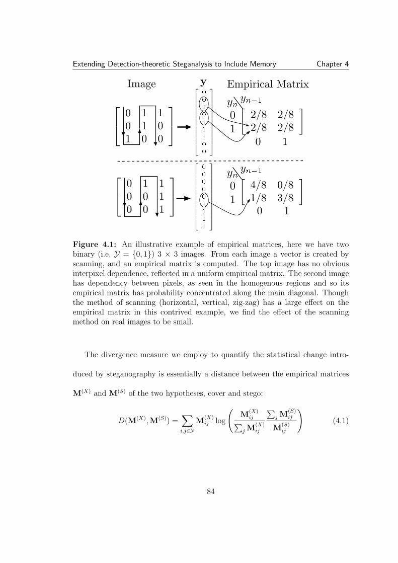
Extending Detection-theoretic Steganalysis to Include Memory Chapter 4
Figure 4.1: An illustrative example of empirical matrices, here we have twobinary (i.e. Y = {0, 1}) 3 × 3 images. From each image a vector is created byscanning, and an empirical matrix is computed. The top image has no obviousinterpixel dependence, reflected in a uniform empirical matrix. The second imagehas dependency between pixels, as seen in the homogenous regions and so itsempirical matrix has probability concentrated along the main diagonal. Thoughthe method of scanning (horizontal, vertical, zig-zag) has a large effect on theempirical matrix in this contrived example, we find the effect of the scanningmethod on real images to be small.
The divergence measure we employ to quantify the statistical change intro-
duced by steganography is essentially a distance between the empirical matrices
M(X) and M(S) of the two hypotheses, cover and stego:
D(M(X),M(S)) =∑i,j∈Y
M(X)ij log
(M
(X)ij∑
j M(X)ij
∑j M
(S)ij
M(S)ij
)(4.1)
84
Extending Detection-theoretic Steganalysis to Include Memory Chapter 4
This divergence has many useful properties for the study of steganalysis in sources
with memory, from the point of view of both the steganographer and the stegan-
alyst.
For a constant false alarm rate, the minimal achievable missed detection rate
approaches e−ND(M(X),M(S)) as N , the number of samples, goes to infinity [64, 1],
just as in the i.i.d. case with K-L divergence. In other words, under the assumption
of a Markov chain model, the performance of the best possible steganalysis is
exponentially bounded by this measure.
It can be seen then that D(M(X),M(S)) provides a measure to the stegano-
grapher of the inherent detectability of a steganographic scheme, given an as-
sumption on the complexity of the detector. This can be seen as an extension
of Cachin’s [10] ε-secure steganography to Markov chains. The gain in using the
Markov chain model is the addition of dependency. In other words, if the detector
in fact uses dependency, an i.i.d. ε-secure hiding scheme overestimates the secrecy
of hiding. To prevent this problem, Chandramouli et al [12] suggest the γD met-
ric. Here the measure of detectability of a steganography method is a bound on
the allowed probabilities of false alarm and missed detection for a given detector
D. While this certainly avoids the problem of underestimating the power of de-
tectors employing dependency, it is only valid with respect to a given detector.
If a different detector is employed, or invented, the security is unknown. The
85
Extending Detection-theoretic Steganalysis to Include Memory Chapter 4
matrix divergence however bounds the false alarm and missed detection probabil-
ities of the best possible detector using one level of dependency. In practice, the
steganographer can choose a scheme that minimizes the divergence for a given
cover joint distribution model (e.g. Gaussian, Laplacian). Alternatively, given a
scheme, the steganographer can choose to use only images that exhibit a small
divergence after hiding.
For the steganalyst, D(M(X),M(S)) measures the amount of information gained
for each additional sample received, just as with the K-L divergence for indepen-
dent samples. The detector can use this to decide if there is enough gain to justify
using a more complex detector. We note that D(M(X),M(S)) is equal to the K-L
divergence if the samples are indeed independent (Mij = pipj):
∑i,j∈Y
M(X)ij log
(M
(X)ij∑
j M(X)ij
∑j M
(S)ij
M(S)ij
)=∑i,j
M(X)ij log
(M
(X)ij
p(X)i
p(S)i
M(S)ij
)
=∑i,j
p(X)i p
(X)j log
(p
(X)i p
(X)j
p(X)i
p(S)i
p(S)i p
(S)j
)
=∑
i
p(X)i
∑j
p(X)j log
p(X)j
p(S)j
=∑
j
p(X)j log
p(X)j
p(S)j
.
Let κ be the ratio of the matrix divergence measure to the K-L divergence. κ
represents the gain of employing the more complex model. For example, to achieve
the same detector power (i.e. same probabilities of miss and false alarm) requires
86

Extending Detection-theoretic Steganalysis to Include Memory Chapter 4
κ times as many samples if the detector uses an i.i.d. cover model versus a MC
model. In the case of independent data, κ is one, and there is no gain to a detector
using statistics beyond a one-dimensional histogram.
4.2.2 Relation to Existing Steganalysis Methods
As mentioned above, using the Markov chain model is analogous to assuming
a complexity constraint on the detector. Since dependency is limited to one ad-
jacent pixel, empirical matrices provide sufficient statistics for optimal detection.
However even two dimensional joint statistics are difficult to use practically. For
practical applications, it is useful to use a subset, or function, of the empirical
matrix. Often these subsets or functions are chosen to match a specific hiding
scheme, and if done correctly do not sacrifice much detection power. However
they certainly cannot improve detection. We now show that many ongoing efforts
in steganalysis use such a subset or function.
Many steganalysis schemes and analysis [21, 69, 46, 35, 84] use a histogram, or
estimate of the one-dimensional PMF, to discriminate between cover and stego.
A one-dimensional histogram is simply the row sums of the empirical matrix:
P (i) =∑
j Mij.
To capture the effect of hiding on interpixel dependencies, some [97, 106] have
used difference histograms, that is, instead of a histogram of sample values, a
87

Extending Detection-theoretic Steganalysis to Include Memory Chapter 4
histogram of the difference of values between samples. As pixels are strongly cor-
related, the difference between pixels is small, and the histogram is concentrated
towards zero. Typically hiding disrupts this concentration, and with appropriate
calibration, the hiding can be detected. The difference histogram is the sums
of the diagonals of the empirical matrix. That is, the difference histogram is
P (x) =∑
i
∑i−j=x Mij. The concentration at zero in the difference histogram
corresponds to the concentration along the main diagonal of the two-dimensional
histogram.
To detect LSB hiding, the RS scheme [33] and related sample-pair analysis [24]
also use counts of differences between pixel values. Though sample-pair analysis
is not limited to adjacent pixels, the authors note the estimate is improved in
practice for spatially adjacent samples. In [72], Roue et al use the empirical
matrix directly to improve the effectiveness of sample-pair analysis.
Also for LSB detection, Sidorov, explicitly using a Markov chain model [78, 79],
uses an entropy-like measure based on ratios of values near the main diagonal of
the empirical matrix:
−2∑i=2
Mi,i−1 logMi,i−1 + Mi,i+1
2Mi,i−1
+ Mi,i+1 logMi,i−1 + Mi,i+1
2Mi,i+1
.
In [34], Fridrich et al use a calibrated blockiness measure to detect Outguess
0.2 [68]. This blockiness measure is the expected value of of the absolute difference
of border pairs, and can be re-written in terms of the empirical matrix generated
88
Extending Detection-theoretic Steganalysis to Include Memory Chapter 4
from pixels straddling 8× 8 block boundaries:
Bl =∑
x=0,1,...
x
∑i
∑|i−j|=x
Mij
.
In [5], Avcibas et al use image quality metrics to measure the effect of hiding.
Though these metrics are not easily related to the empirical matrix, it is notable
that the metrics are evaluated between the image under scrutiny, and a low-
pass filtered version of the image. To generate the filtered image, each pixel is
replaced with a weighted sum of a 3×3 neighborhood surrounding the pixel. In
other words, it is assumed that the measurable difference between a given image
and the same image with artificially enhanced interpixel dependencies is different
for stego images and cover images.
We have argued that analysis using a Markov chain model provides meaningful
results under the condition of a steganalyst incorporating one level of dependency
for detection. We have seen here that many existing detection methods indeed
implicitly employ such a model.
Due to the lack of information available to the steganalyst, practical detection
is inevitably suboptimal. However we still expect some relationship between the
calculated divergence and the efficacy of state-of-the-art steganalysis. In the fol-
lowing section, we examine the divergence measure two existing steganographic
schemes, and compare with current detection methods to test this assumption.
89
Extending Detection-theoretic Steganalysis to Include Memory Chapter 4
Additionally we compare the calculated divergence under an assumption of inde-
pendence (Eqn. (3.2)) to the divergence assuming dependency (Eqn. (4.1)) to
evaluate the value to the steganalyst in incorporating a more complex statistical
model.
4.3 Spread Spectrum
As noted in Chapter 2, spread spectrum data hiding (SS) [19] is an estab-
lished embedding method, often used for watermarking, but also applicable for
steganography [60]. We here measure and study the statistical effect of hiding on
the empirical matrix, and relate this to detection experiments we performed.
4.3.1 Measuring Detectability of Hiding
In spread spectrum data hiding, the message data modulates a noise sequence
to create a message bearing signal, which is then added to the cover data. Since its
introduction, many variants of SS have been proposed, typically in the context of
watermarking. The major goal in watermarking is robustness to malicious attacks,
rather than statistical invisibility. We therefore focus on three basic models of
hiding suggested by Cox et al, shown here for reference. Let {Dk, k ≥ 0} be a
zero mean, unit variance, Gaussian message bearing signal, and {Xk,≥ 0} be the
90
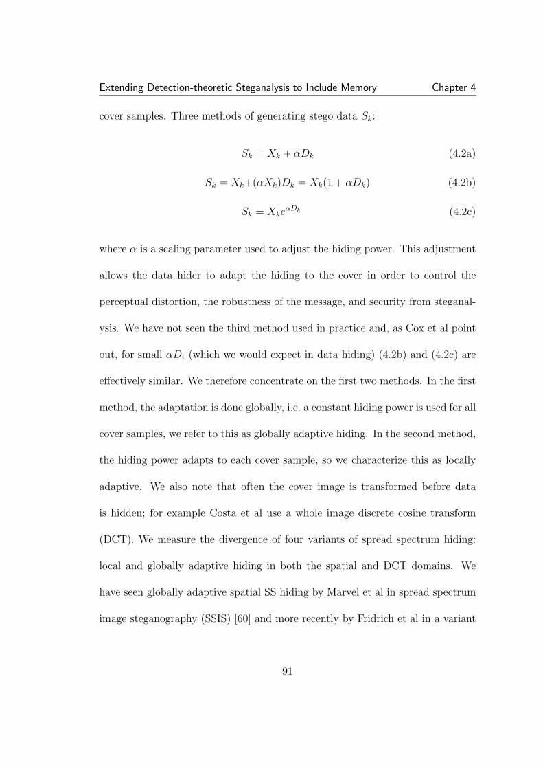
Extending Detection-theoretic Steganalysis to Include Memory Chapter 4
cover samples. Three methods of generating stego data Sk:
Sk = Xk + αDk (4.2a)
Sk = Xk+(αXk)Dk = Xk(1 + αDk) (4.2b)
Sk = XkeαDk (4.2c)
where α is a scaling parameter used to adjust the hiding power. This adjustment
allows the data hider to adapt the hiding to the cover in order to control the
perceptual distortion, the robustness of the message, and security from steganal-
ysis. We have not seen the third method used in practice and, as Cox et al point
out, for small αDi (which we would expect in data hiding) (4.2b) and (4.2c) are
effectively similar. We therefore concentrate on the first two methods. In the first
method, the adaptation is done globally, i.e. a constant hiding power is used for all
cover samples, we refer to this as globally adaptive hiding. In the second method,
the hiding power adapts to each cover sample, so we characterize this as locally
adaptive. We also note that often the cover image is transformed before data
is hidden; for example Costa et al use a whole image discrete cosine transform
(DCT). We measure the divergence of four variants of spread spectrum hiding:
local and globally adaptive hiding in both the spatial and DCT domains. We
have seen globally adaptive spatial SS hiding by Marvel et al in spread spectrum
image steganography (SSIS) [60] and more recently by Fridrich et al in a variant
91

Extending Detection-theoretic Steganalysis to Include Memory Chapter 4
of stochastic modulation [31]. The latter allows for a higher number of bits to be
successfully decoded and the capacity is a function of the message signal power.
The experiments presented by Cox et al [19] are locally adaptive DCT hiding.
For each variant we calculated the divergence over a range of message signal
power. For globally adaptive hiding we hold the message to cover power ratio
(MCR) constant. In the locally adaptive case this is not possible so we hold the
scale factor α constant. The MCR varies from image to image; we record the
average value with the data.
To generalize our approach we would like to simplify the divergence mea-
surement, by eliminating the need to derive the stego empirical matrix. Instead
of using statistical analysis of the hiding scheme to generate an expected stego
empirical matrix, Monte Carlo simulations of data hiding in several images may
provide an accurate means of estimating divergence. To do this, several synthetic
images are generated from the empirical matrix of a cover image. Data is hidden
in these synthetic images, and stego empirical matrices are calculated from the
resulting images. The average divergence between these empirical matrices and
the original cover matrix represent an estimate of the divergence introduced by
hiding
As mentioned in Section 4.2.1, the divergence measure provides to the stega-
nographer a benchmark of the inherent detectability of hiding. Additionally, it
92
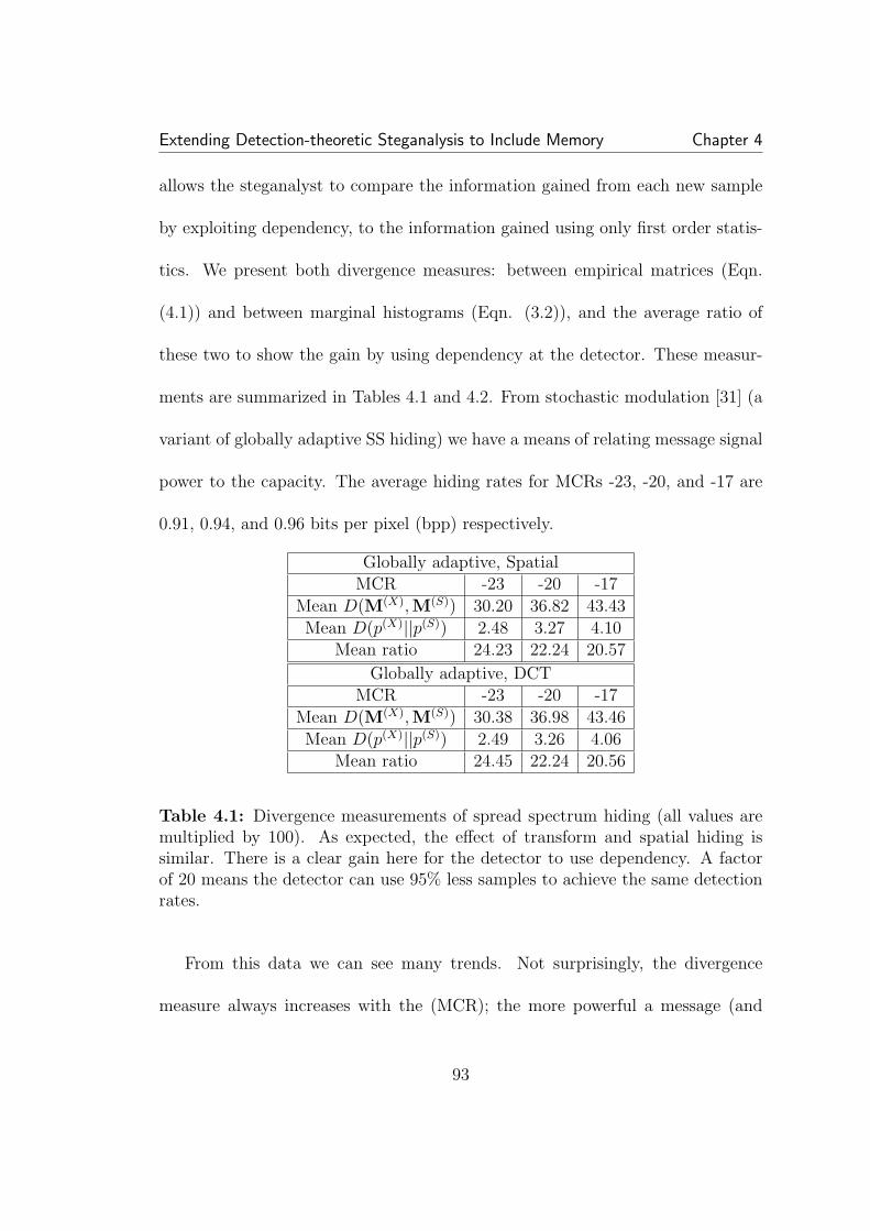
Extending Detection-theoretic Steganalysis to Include Memory Chapter 4
allows the steganalyst to compare the information gained from each new sample
by exploiting dependency, to the information gained using only first order statis-
tics. We present both divergence measures: between empirical matrices (Eqn.
(4.1)) and between marginal histograms (Eqn. (3.2)), and the average ratio of
these two to show the gain by using dependency at the detector. These measur-
ments are summarized in Tables 4.1 and 4.2. From stochastic modulation [31] (a
variant of globally adaptive SS hiding) we have a means of relating message signal
power to the capacity. The average hiding rates for MCRs -23, -20, and -17 are
0.91, 0.94, and 0.96 bits per pixel (bpp) respectively.
Globally adaptive, SpatialMCR -23 -20 -17
Mean D(M(X),M(S)) 30.20 36.82 43.43
Mean D(p(X)||p(S)) 2.48 3.27 4.10Mean ratio 24.23 22.24 20.57
Globally adaptive, DCTMCR -23 -20 -17
Mean D(M(X),M(S)) 30.38 36.98 43.46
Mean D(p(X)||p(S)) 2.49 3.26 4.06Mean ratio 24.45 22.24 20.56
Table 4.1: Divergence measurements of spread spectrum hiding (all values aremultiplied by 100). As expected, the effect of transform and spatial hiding issimilar. There is a clear gain here for the detector to use dependency. A factorof 20 means the detector can use 95% less samples to achieve the same detectionrates.
From this data we can see many trends. Not surprisingly, the divergence
measure always increases with the (MCR); the more powerful a message (and
93
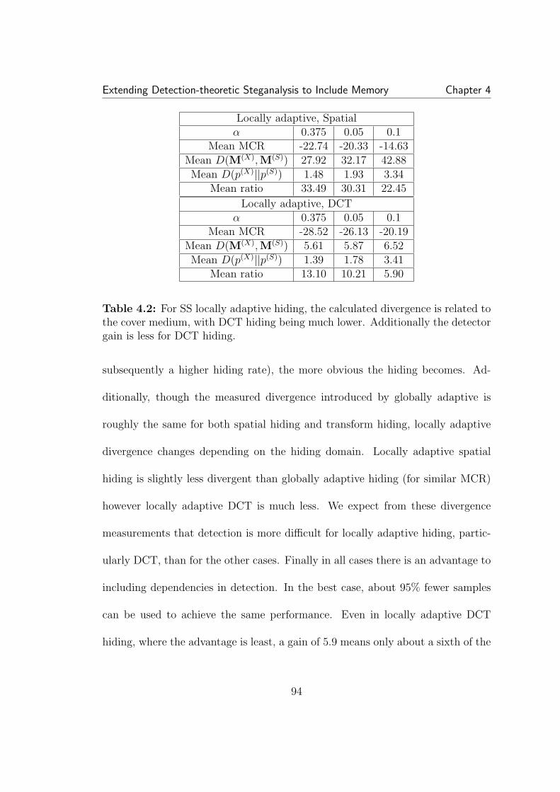
Extending Detection-theoretic Steganalysis to Include Memory Chapter 4
Locally adaptive, Spatialα 0.375 0.05 0.1
Mean MCR -22.74 -20.33 -14.63
Mean D(M(X),M(S)) 27.92 32.17 42.88
Mean D(p(X)||p(S)) 1.48 1.93 3.34Mean ratio 33.49 30.31 22.45
Locally adaptive, DCTα 0.375 0.05 0.1
Mean MCR -28.52 -26.13 -20.19
Mean D(M(X),M(S)) 5.61 5.87 6.52
Mean D(p(X)||p(S)) 1.39 1.78 3.41Mean ratio 13.10 10.21 5.90
Table 4.2: For SS locally adaptive hiding, the calculated divergence is related tothe cover medium, with DCT hiding being much lower. Additionally the detectorgain is less for DCT hiding.
subsequently a higher hiding rate), the more obvious the hiding becomes. Ad-
ditionally, though the measured divergence introduced by globally adaptive is
roughly the same for both spatial hiding and transform hiding, locally adaptive
divergence changes depending on the hiding domain. Locally adaptive spatial
hiding is slightly less divergent than globally adaptive hiding (for similar MCR)
however locally adaptive DCT is much less. We expect from these divergence
measurements that detection is more difficult for locally adaptive hiding, partic-
ularly DCT, than for the other cases. Finally in all cases there is an advantage to
including dependencies in detection. In the best case, about 95% fewer samples
can be used to achieve the same performance. Even in locally adaptive DCT
hiding, where the advantage is least, a gain of 5.9 means only about a sixth of the
94
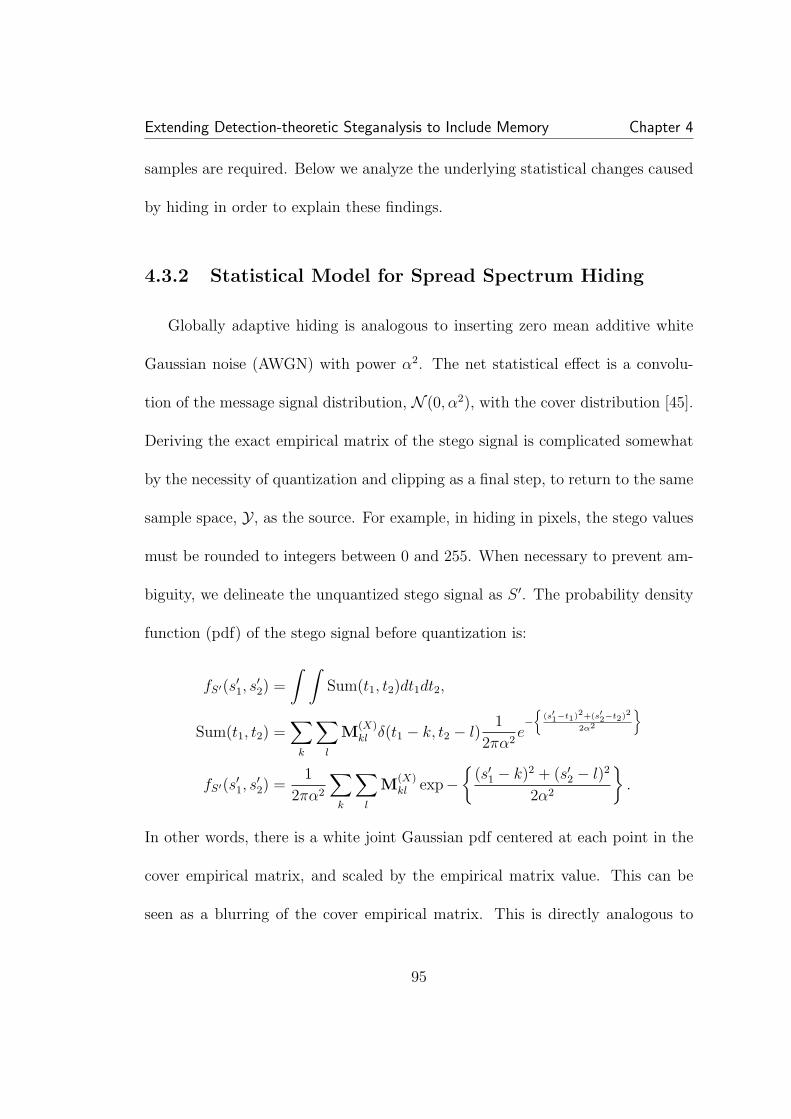
Extending Detection-theoretic Steganalysis to Include Memory Chapter 4
samples are required. Below we analyze the underlying statistical changes caused
by hiding in order to explain these findings.
4.3.2 Statistical Model for Spread Spectrum Hiding
Globally adaptive hiding is analogous to inserting zero mean additive white
Gaussian noise (AWGN) with power α2. The net statistical effect is a convolu-
tion of the message signal distribution, N (0, α2), with the cover distribution [45].
Deriving the exact empirical matrix of the stego signal is complicated somewhat
by the necessity of quantization and clipping as a final step, to return to the same
sample space, Y , as the source. For example, in hiding in pixels, the stego values
must be rounded to integers between 0 and 255. When necessary to prevent am-
biguity, we delineate the unquantized stego signal as S ′. The probability density
function (pdf) of the stego signal before quantization is:
fS′(s′1, s′2) =
∫ ∫Sum(t1, t2)dt1dt2,
Sum(t1, t2) =∑
k
∑l
M(X)kl δ(t1 − k, t2 − l)
1
2πα2e−
(s′1−t1)2+(s′2−t2)2
2α2
ff
fS′(s′1, s′2) =
1
2πα2
∑k
∑l
M(X)kl exp−
{(s′1 − k)2 + (s′2 − l)2
2α2
}.
In other words, there is a white joint Gaussian pdf centered at each point in the
cover empirical matrix, and scaled by the empirical matrix value. This can be
seen as a blurring of the cover empirical matrix. This is directly analogous to
95
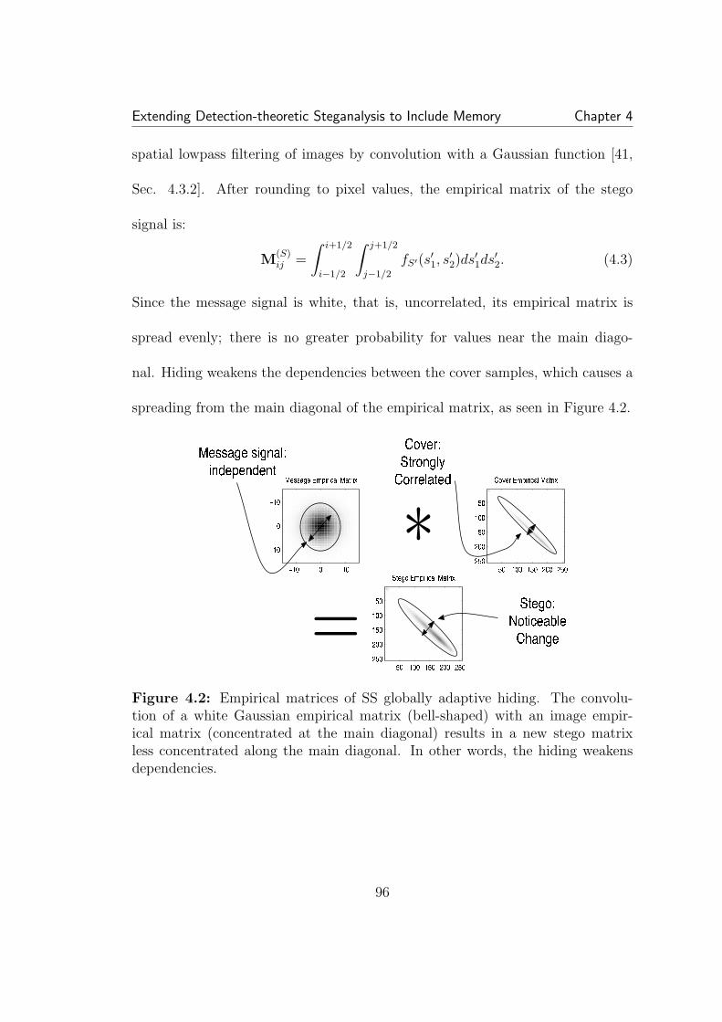
Extending Detection-theoretic Steganalysis to Include Memory Chapter 4
spatial lowpass filtering of images by convolution with a Gaussian function [41,
Sec. 4.3.2]. After rounding to pixel values, the empirical matrix of the stego
signal is:
M(S)ij =
∫ i+1/2
i−1/2
∫ j+1/2
j−1/2
fS′(s′1, s′2)ds′1ds′2. (4.3)
Since the message signal is white, that is, uncorrelated, its empirical matrix is
spread evenly; there is no greater probability for values near the main diago-
nal. Hiding weakens the dependencies between the cover samples, which causes a
spreading from the main diagonal of the empirical matrix, as seen in Figure 4.2.
Figure 4.2: Empirical matrices of SS globally adaptive hiding. The convolu-tion of a white Gaussian empirical matrix (bell-shaped) with an image empir-ical matrix (concentrated at the main diagonal) results in a new stego matrixless concentrated along the main diagonal. In other words, the hiding weakensdependencies.
96
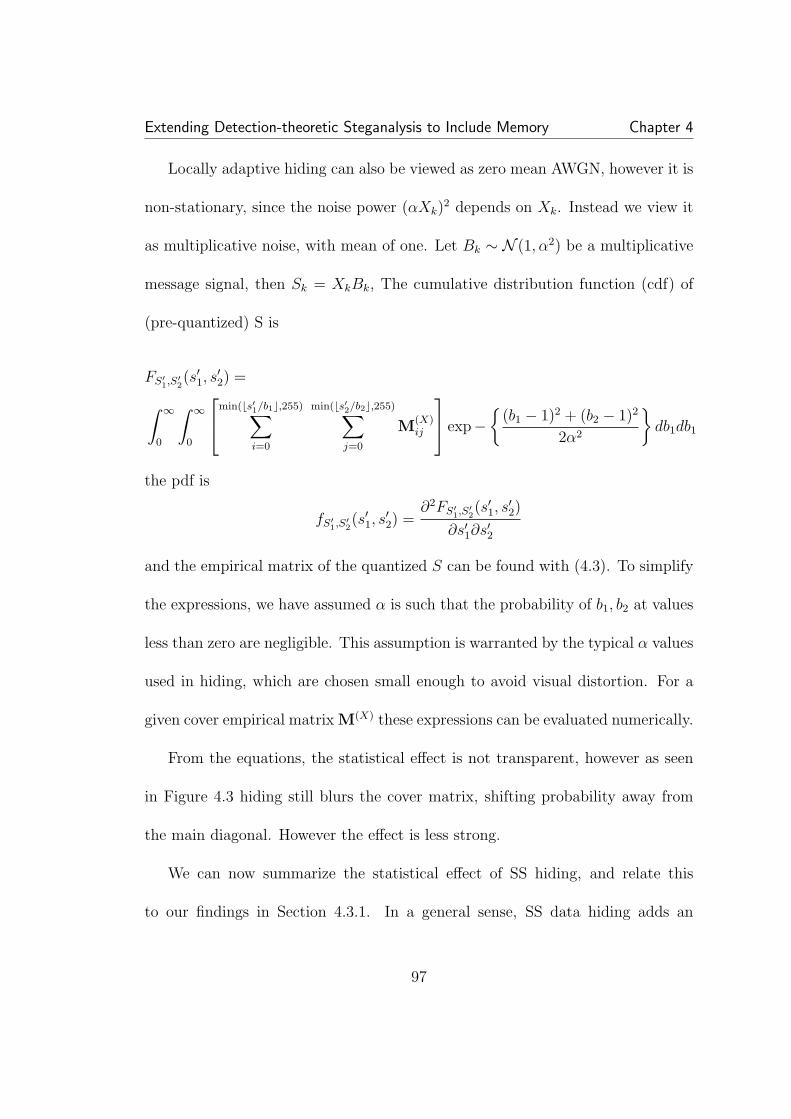
Extending Detection-theoretic Steganalysis to Include Memory Chapter 4
Locally adaptive hiding can also be viewed as zero mean AWGN, however it is
non-stationary, since the noise power (αXk)2 depends on Xk. Instead we view it
as multiplicative noise, with mean of one. Let Bk ∼ N (1, α2) be a multiplicative
message signal, then Sk = XkBk, The cumulative distribution function (cdf) of
(pre-quantized) S is
FS′1,S′
2(s′1, s
′2) =∫ ∞
0
∫ ∞
0
min(bs′1/b1c,255)∑i=0
min(bs′2/b2c,255)∑j=0
M(X)ij
exp−{
(b1 − 1)2 + (b2 − 1)2
2α2
}db1db1
the pdf is
fS′1,S′
2(s′1, s
′2) =
∂2FS′1,S′
2(s′1, s
′2)
∂s′1∂s′2
and the empirical matrix of the quantized S can be found with (4.3). To simplify
the expressions, we have assumed α is such that the probability of b1, b2 at values
less than zero are negligible. This assumption is warranted by the typical α values
used in hiding, which are chosen small enough to avoid visual distortion. For a
given cover empirical matrix M(X) these expressions can be evaluated numerically.
From the equations, the statistical effect is not transparent, however as seen
in Figure 4.3 hiding still blurs the cover matrix, shifting probability away from
the main diagonal. However the effect is less strong.
We can now summarize the statistical effect of SS hiding, and relate this
to our findings in Section 4.3.1. In a general sense, SS data hiding adds an
97
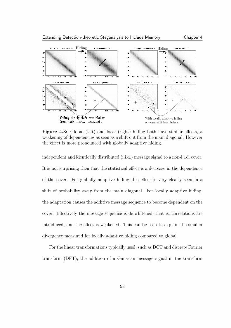
Extending Detection-theoretic Steganalysis to Include Memory Chapter 4
Figure 4.3: Global (left) and local (right) hiding both have similar effects, aweakening of dependencies as seen as a shift out from the main diagonal. Howeverthe effect is more pronounced with globally adaptive hiding.
independent and identically distributed (i.i.d.) message signal to a non-i.i.d. cover.
It is not surprising then that the statistical effect is a decrease in the dependence
of the cover. For globally adaptive hiding this effect is very clearly seen in a
shift of probability away from the main diagonal. For locally adaptive hiding,
the adaptation causes the additive message sequence to become dependent on the
cover. Effectively the message sequence is de-whitened, that is, correlations are
introduced, and the effect is weakened. This can be seen to explain the smaller
divergence measured for locally adaptive hiding compared to global.
For the linear transformations typically used, such as DCT and discrete Fourier
transform (DFT), the addition of a Gaussian message signal in the transform
98
Extending Detection-theoretic Steganalysis to Include Memory Chapter 4
domain is equivalent to adding a Gaussian message signal in the spatial domain.
So globally adaptive hiding in DCT coefficients statistically has the same effect
as hiding in pixels. However, locally adaptive hiding is effectively a multiplicative
Gaussian signal, which is not equivalent in both domains. This helps explain why
the calculated divergence was nearly equal for globally adaptive hiding in either
domain, but differed greatly for locally adaptive hiding.
Finally we found the most noticeable effect of spread spectrum hiding is a
spreading from the main diagonal of the empirical matrix. Since the histogram
is just the collection of sums of each row of the empirical matrix, this effect is
missed by studying only marginal statistics. That is, the spreading along each
row is not visible when the row is summed into a single point. This explains the
gain of using dependency in detection.
4.3.3 Practical Detection
We now compare the measurements of the optimal detectability of SS hiding
to experiments using a practical detector. We find the practical experiments
follow the estimates above. We also compare experiments for a detector using
dependencies with a simpler detector to judge the expected gain in detection.
To achieve optimal detection of data hiding, the detection-theoretic prescrip-
tion is to calculate the empirical matrix of a suspected image and calculate the
99

Extending Detection-theoretic Steganalysis to Include Memory Chapter 4
divergence between this and the empirical matrices of both the cover and the
stego. Whichever is “closer”, i.e. has a smaller divergence measurement, is the
optimal decision. From the analysis above we can evaluate the stego empirical
matrix given the cover matrix. The cover statistics however are not known in a
practical scenario. As with QIM detection in Section 3.3.3 we turn to supervised
learning to overcome our lack of knowledge.
For the experiments we need an image database, a learning algorithm, and a
feature vector to train the machine. In the image database, we want to represent
the vast variety of real images as well as possible. We expand our previous image
set to a mix of four separate sources:
1. digital camera images, partitioned into smaller sub-images
2. scanned photographs
3. scanned, downsampled, and cropped photographs
4. images from the Corel volume Scenic Sites
All images are converted losslessly to PNG format and color images are converted
to grayscale. The entire database is approximately 1400 images. Half of these are
used for training and half for testing. Within both the training and testing sets,
half are cover images and half are (distinct) stego images.
100
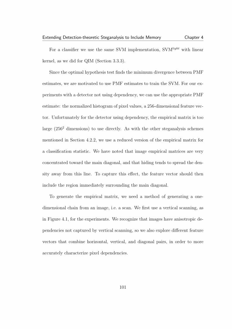
Extending Detection-theoretic Steganalysis to Include Memory Chapter 4
For a classifier we use the same SVM implementation, SVMlight with linear
kernel, as we did for QIM (Section 3.3.3).
Since the optimal hypothesis test finds the minimum divergence between PMF
estimates, we are motivated to use PMF estimates to train the SVM. For our ex-
periments with a detector not using dependency, we can use the appropriate PMF
estimate: the normalized histogram of pixel values, a 256-dimensional feature vec-
tor. Unfortunately for the detector using dependency, the empirical matrix is too
large (2562 dimensions) to use directly. As with the other steganalysis schemes
mentioned in Section 4.2.2, we use a reduced version of the empirical matrix for
a classification statistic. We have noted that image empirical matrices are very
concentrated toward the main diagonal, and that hiding tends to spread the den-
sity away from this line. To capture this effect, the feature vector should then
include the region immediately surrounding the main diagonal.
To generate the empirical matrix, we need a method of generating a one-
dimensional chain from an image, i.e. a scan. We first use a vertical scanning, as
in Figure 4.1, for the experiments. We recognize that images have anisotropic de-
pendencies not captured by vertical scanning, so we also explore different feature
vectors that combine horizontal, vertical, and diagonal pairs, in order to more
accurately characterize pixel dependencies.
101

Extending Detection-theoretic Steganalysis to Include Memory Chapter 4
For an empirical matrix M calculated from an image, first the 6 highest prob-
abilities on the main diagonal (Mii) are chosen, and for each of these the following
10 nearest differences are picked:
{Mi,i, Mi,i−1, Mi,i−2, . . . ,Mi,i−10}
All together this gives a 66-dimensional vector. We wish to also capture changes
along the center line. To do this we subsample the remaining main diagonal values
by four:
{M1,1, M5,5, M9,9, . . . ,M253,253}
see Figure 4.4. The resulting total feature vector is 129-dimensional, a manage-
able size that still captures much of the hiding effect. A comparison of the feature
vectors used to evaluate the performance of both detectors, using and not using
dependencies, is shown in Figure 4.5. In addition to generating an empirical
matrix based on adjacent pixels, we experimented with an empirical matrix gen-
erated from a pixel and an average of its four nearest neighbors. This is done in
an attempt to capture a possible gain to using a more complex model, while still
falling into our framework.
We tested the same four SS variants as in the previous sections. To relate these
experiments to other work done, we based our hiding power on that reported in
the literature. Spread spectrum image steganography (SSIS) [60] is an implemen-
102
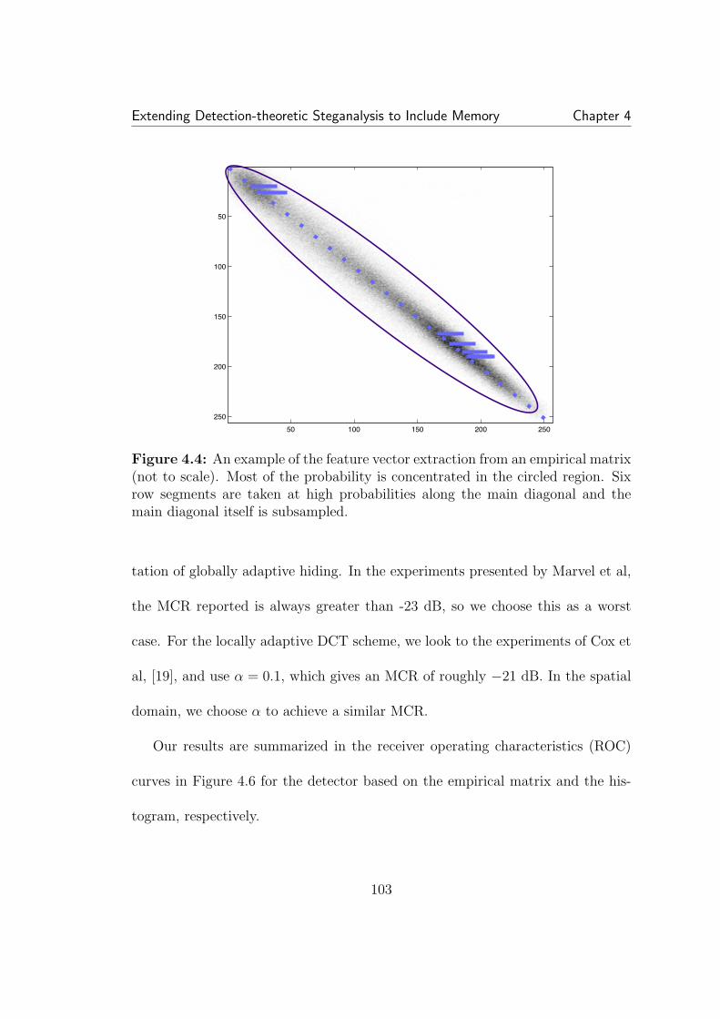
Extending Detection-theoretic Steganalysis to Include Memory Chapter 4
50 100 150 200 250
50
100
150
200
250
Figure 4.4: An example of the feature vector extraction from an empirical matrix(not to scale). Most of the probability is concentrated in the circled region. Sixrow segments are taken at high probabilities along the main diagonal and themain diagonal itself is subsampled.
tation of globally adaptive hiding. In the experiments presented by Marvel et al,
the MCR reported is always greater than -23 dB, so we choose this as a worst
case. For the locally adaptive DCT scheme, we look to the experiments of Cox et
al, [19], and use α = 0.1, which gives an MCR of roughly −21 dB. In the spatial
domain, we choose α to achieve a similar MCR.
Our results are summarized in the receiver operating characteristics (ROC)
curves in Figure 4.6 for the detector based on the empirical matrix and the his-
togram, respectively.
103
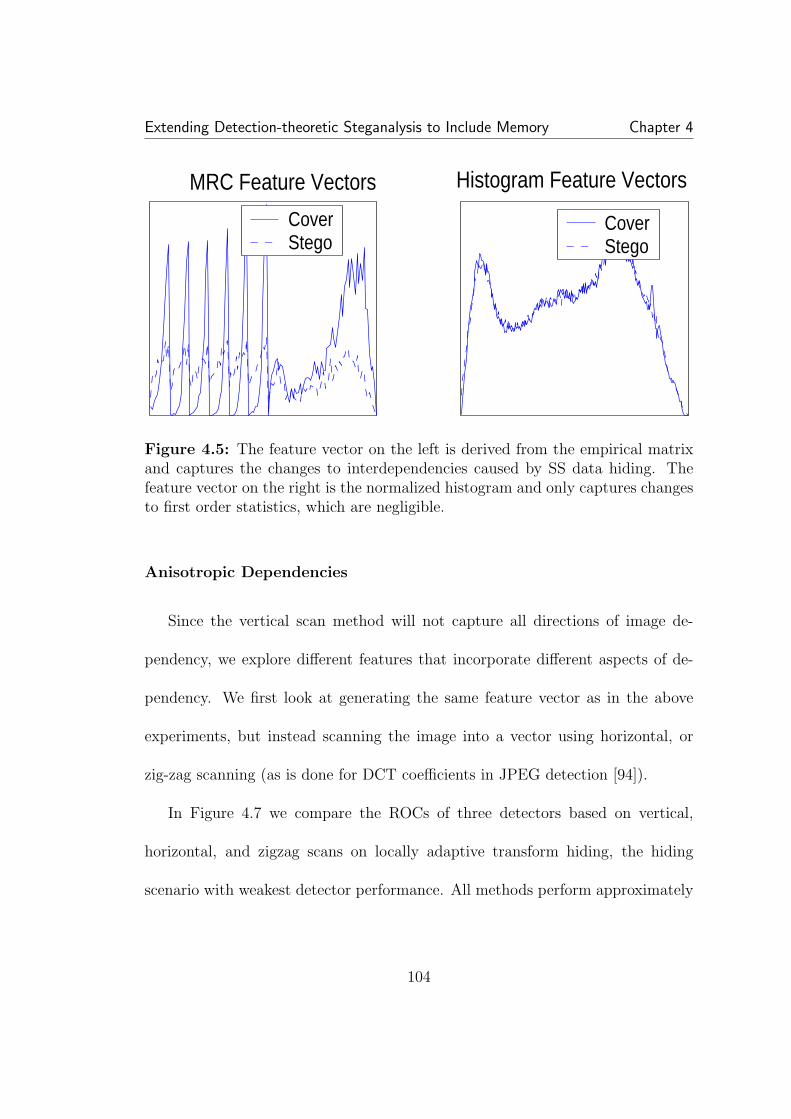
Extending Detection-theoretic Steganalysis to Include Memory Chapter 4
MRC Feature Vectors Histogram Feature Vectors
CoverStego
CoverStego
Figure 4.5: The feature vector on the left is derived from the empirical matrixand captures the changes to interdependencies caused by SS data hiding. Thefeature vector on the right is the normalized histogram and only captures changesto first order statistics, which are negligible.
Anisotropic Dependencies
Since the vertical scan method will not capture all directions of image de-
pendency, we explore different features that incorporate different aspects of de-
pendency. We first look at generating the same feature vector as in the above
experiments, but instead scanning the image into a vector using horizontal, or
zig-zag scanning (as is done for DCT coefficients in JPEG detection [94]).
In Figure 4.7 we compare the ROCs of three detectors based on vertical,
horizontal, and zigzag scans on locally adaptive transform hiding, the hiding
scenario with weakest detector performance. All methods perform approximately
104
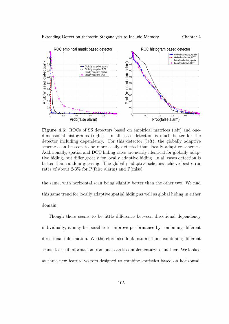
Extending Detection-theoretic Steganalysis to Include Memory Chapter 4
0 0.2 0.4 0.6 0.8 10
0.1
0.2
0.3
0.4
0.5
0.6
0.7
0.8
0.9
1ROC empirical matrix based detector
Prob(false alarm)
Pro
b(m
isse
d d
ete
ctio
n)
Globally adaptive, spatialGlobally adaptive, DCTLocally adaptive, spatialLocally adaptive, DCT
0 0.2 0.4 0.6 0.8 10
0.1
0.2
0.3
0.4
0.5
0.6
0.7
0.8
0.9
1ROC histogram based detector
Prob(false alarm)
Pro
b(m
isse
d d
ete
ctio
n)
Globally adaptive, spatialGlobally adaptive, DCTLocally adaptive, spatialLocally adaptive, DCT
Figure 4.6: ROCs of SS detectors based on empirical matrices (left) and one-dimensional histograms (right). In all cases detection is much better for thedetector including dependency. For this detector (left), the globally adaptiveschemes can be seen to be more easily detected than locally adaptive schemes.Additionally, spatial and DCT hiding rates are nearly identical for globally adap-tive hiding, but differ greatly for locally adaptive hiding. In all cases detection isbetter than random guessing. The globally adaptive schemes achieve best errorrates of about 2-3% for P(false alarm) and P(miss).
the same, with horizontal scan being slightly better than the other two. We find
this same trend for locally adaptive spatial hiding as well as global hiding in either
domain.
Though there seems to be little difference between directional dependency
individually, it may be possible to improve performance by combining different
directional information. We therefore also look into methods combining different
scans, to see if information from one scan is complementary to another. We looked
at three new feature vectors designed to combine statistics based on horizontal,
105
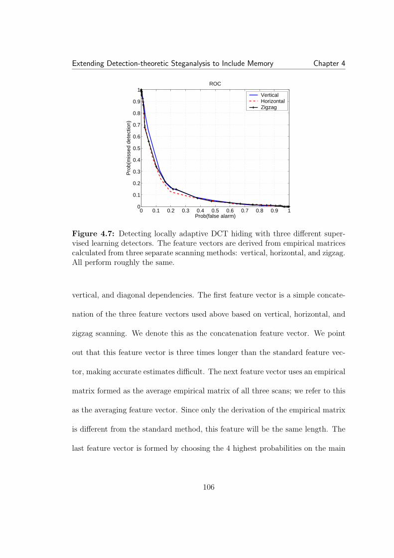
Extending Detection-theoretic Steganalysis to Include Memory Chapter 4
0 0.1 0.2 0.3 0.4 0.5 0.6 0.7 0.8 0.9 10
0.1
0.2
0.3
0.4
0.5
0.6
0.7
0.8
0.9
1ROC
Prob(false alarm)
Pro
b(m
isse
d de
tect
ion)
VerticalHorizontalZigzag
Figure 4.7: Detecting locally adaptive DCT hiding with three different super-vised learning detectors. The feature vectors are derived from empirical matricescalculated from three separate scanning methods: vertical, horizontal, and zigzag.All perform roughly the same.
vertical, and diagonal dependencies. The first feature vector is a simple concate-
nation of the three feature vectors used above based on vertical, horizontal, and
zigzag scanning. We denote this as the concatenation feature vector. We point
out that this feature vector is three times longer than the standard feature vec-
tor, making accurate estimates difficult. The next feature vector uses an empirical
matrix formed as the average empirical matrix of all three scans; we refer to this
as the averaging feature vector. Since only the derivation of the empirical matrix
is different from the standard method, this feature will be the same length. The
last feature vector is formed by choosing the 4 highest probabilities on the main
106

Extending Detection-theoretic Steganalysis to Include Memory Chapter 4
diagonal of each of the three individual empirical matrices, and choosing the 10
nearest differences. Recall that the standard feature vector chooses the 10 nearest
differences of the top 6 probabilities, and additionally includes a sub-sampling of
the main diagonal. So this final feature vector takes sections we believe to con-
tain the most information from each of the three different scanning vectors. This
final feature vector, denoted as cut-and-paste feature vector, is 132-dimensional,
nearly the same as the standard 129-dimensional vector. In Figure 4.8 we compare
the detector performance on locally adaptive hiding in the spatial and transform
domains. For hiding in DCT coefficients, all the detectors perform roughly the
same. The three feature vectors combining vertical, horizontal, and zigzag scans
perform nominally worse than the standard vector based on horizontal scanning
alone. So, although more information is accounted for, there is no gain in using
these combined feature vectors (more on this presently). We find these same rel-
ative performance characteristics for globally adaptive spatial and DCT hiding.
For locally adaptive spatial hiding however, we found the cut-and-paste feature
vector to perform much worse than the others. The cut-and-paste feature vector
does not include as much information from the main diagonal of the empirical
matrix. It can be inferred then that changes to the main diagonal are important
to detection of locally adaptive spatial hiding.
107
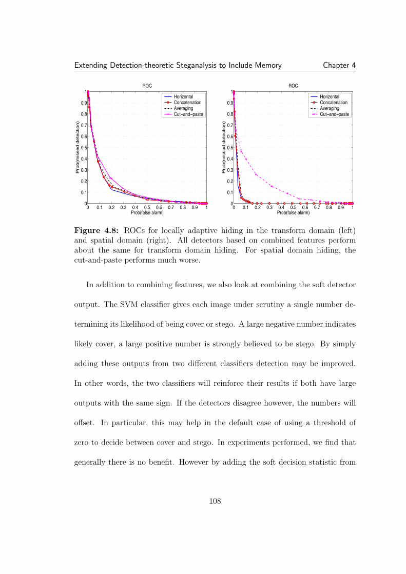
Extending Detection-theoretic Steganalysis to Include Memory Chapter 4
0 0.1 0.2 0.3 0.4 0.5 0.6 0.7 0.8 0.9 10
0.1
0.2
0.3
0.4
0.5
0.6
0.7
0.8
0.9
1ROC
Prob(false alarm)
Pro
b(m
issed d
ete
ction)
HorizontalConcatenationAveragingCut−and−paste
0 0.1 0.2 0.3 0.4 0.5 0.6 0.7 0.8 0.9 10
0.1
0.2
0.3
0.4
0.5
0.6
0.7
0.8
0.9
1ROC
Prob(false alarm)
Pro
b(m
issed d
ete
ction)
HorizontalConcatenationAveragingCut−and−paste
Figure 4.8: ROCs for locally adaptive hiding in the transform domain (left)and spatial domain (right). All detectors based on combined features performabout the same for transform domain hiding. For spatial domain hiding, thecut-and-paste performs much worse.
In addition to combining features, we also look at combining the soft detector
output. The SVM classifier gives each image under scrutiny a single number de-
termining its likelihood of being cover or stego. A large negative number indicates
likely cover, a large positive number is strongly believed to be stego. By simply
adding these outputs from two different classifiers detection may be improved.
In other words, the two classifiers will reinforce their results if both have large
outputs with the same sign. If the detectors disagree however, the numbers will
offset. In particular, this may help in the default case of using a threshold of
zero to decide between cover and stego. In experiments performed, we find that
generally there is no benefit. However by adding the soft decision statistic from
108

Extending Detection-theoretic Steganalysis to Include Memory Chapter 4
classifiers based on the horizontal scan feature vector and the cut-and-paste fea-
ture vector, better zero threshold performance is acquired for detection of globally
adaptive schemes than any other classifier we use, see Table 4.3
Hiding Method Horizontal Cut-and-paste SummedP(f.a.) P(miss) P(f.a.) P(miss) P(f.a.) P(miss)
Global adapt., spatial 0.050 0.012 0.050 0.053 0.036 0.012Global adapt., DCT 0.041 0.006 0.050 0.003 0.011 0
Table 4.3: A comparison of the classifier performance based on comparing threedifferent soft decision statistics to a zero threshold: the output of a classifier usinga feature vector derived from horizontal image scanning; the output of a classifierusing the cut-and-paste feature vector described above, and the sum of these two.In this particular case, adding the soft classifier output before comparing to zerothreshold achieves better detection than either individual case.
Finally, we compare the results of the detector based on the empirical matrix
based on one adjacent pixel, and that generated from an average of four adjacent
pixels. In Figure 4.9, we compare the results of both detectors for locally adaptive
DCT hiding; the results for the other three variants are similar. The detectors
perform closely, suggesting the simple Markov chain model captures the important
changes introduced by hiding.
Comparison
We note that our results for detecting spatial globally adaptive hiding, error
rates on the order of 1 to 5%, are similar to those of Harmsen and Pearlman
in [45] detecting SSIS in color images. For detection they used a statistic based
109
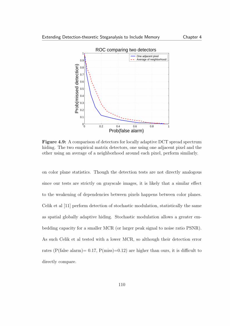
Extending Detection-theoretic Steganalysis to Include Memory Chapter 4
0 0.2 0.4 0.6 0.8 10
0.1
0.2
0.3
0.4
0.5
0.6
0.7
0.8
0.9
1ROC comparing two detectors
Prob(false alarm)
Pro
b(m
isse
d d
ete
ctio
n)
One adjacent pixelAverage of neighborhood
Figure 4.9: A comparison of detectors for locally adaptive DCT spread spectrumhiding. The two empirical matrix detectors, one using one adjacent pixel and theother using an average of a neighborhood around each pixel, perform similarly.
on color plane statistics. Though the detection tests are not directly analogous
since our tests are strictly on grayscale images, it is likely that a similar effect
to the weakening of dependencies between pixels happens between color planes.
Celik et al [11] perform detection of stochastic modulation, statistically the same
as spatial globally adaptive hiding. Stochastic modulation allows a greater em-
bedding capacity for a smaller MCR (or larger peak signal to noise ratio PSNR).
As such Celik et al tested with a lower MCR, so although their detection error
rates (P(false alarm)= 0.17, P(miss)=0.12) are higher than ours, it is difficult to
directly compare.
110
Extending Detection-theoretic Steganalysis to Include Memory Chapter 4
4.3.4 SS Hiding Conclusion
We find the results of a practical detector matches that which our divergence
measurements and analysis led us to expect. For the steganographer it may first
seem that locally adaptive DCT hiding is the superior choice for hiding. However
there are two important points to mention: First, unlike globally adaptive hiding,
locally adaptive hiding only meets a target MCR on average. The MCR for
each image varies and this may make detection more difficult. Second, although
the globally adaptive hiding rate is a function of the message signal power, the
locally adaptive hiding rate is not readily available, and may in fact be less than
globally adaptive hiding for a given MCR. In all cases there is clearly a gain to
the steganalyst to using a model of dependency for detection. In the following
section we perform a similar analysis to a hiding scheme specifically designed to
evade detection.
4.4 JPEG Perturbation Quantization
Recently Fridrich et al [38] introduced an implementation of their perturba-
tion quantization hiding method that creates stego images that mimic a double-
compressed clean image. We measure the divergence of this method and show
these are related to practical detection results presented by Kharrazi et al [53]. As
111
Extending Detection-theoretic Steganalysis to Include Memory Chapter 4
with spread spectrum hiding, we study the statistical effect of hiding to explain
these findings.
4.4.1 Measuring Detectability of Hiding
As the name implies, perturbation quantization is a variant of quantization
index modulation (QIM) [14]. Standard QIM hiding in JPEG images has a dis-
tinctive statistical effect, and we have shown in Section 3.3 that it can be detected.
Double compressed PQ however is specifically contrived to minimize the statis-
tical difference between the stego image, and an image that has simply been
compressed twice. This is achieved by embedding in coefficients that ideally have
the same distribution after a second compression as they do by data hiding.
In [53], Kharrazi et al measure the detection rates for three blind methods
of steganalysis used on a variety of steganography schemes. The term “cover” is
somewhat ambiguous for PQ JPEG hiding. The original source, from which the
stego image is generated, is a once compressed image. However PQ is designed
to mimic twice compressed images, which the authors argue occur naturally [38].
Because of this ambiguity, Kharrazi et al measure the detection rates of two cases:
comparing with the source (single-compressed) images, and comparing with re-
compressed (i.e. double-compressed) images. For the first case, detection is found
to be possible, but by no means certain. For example, in one case the sum of
112
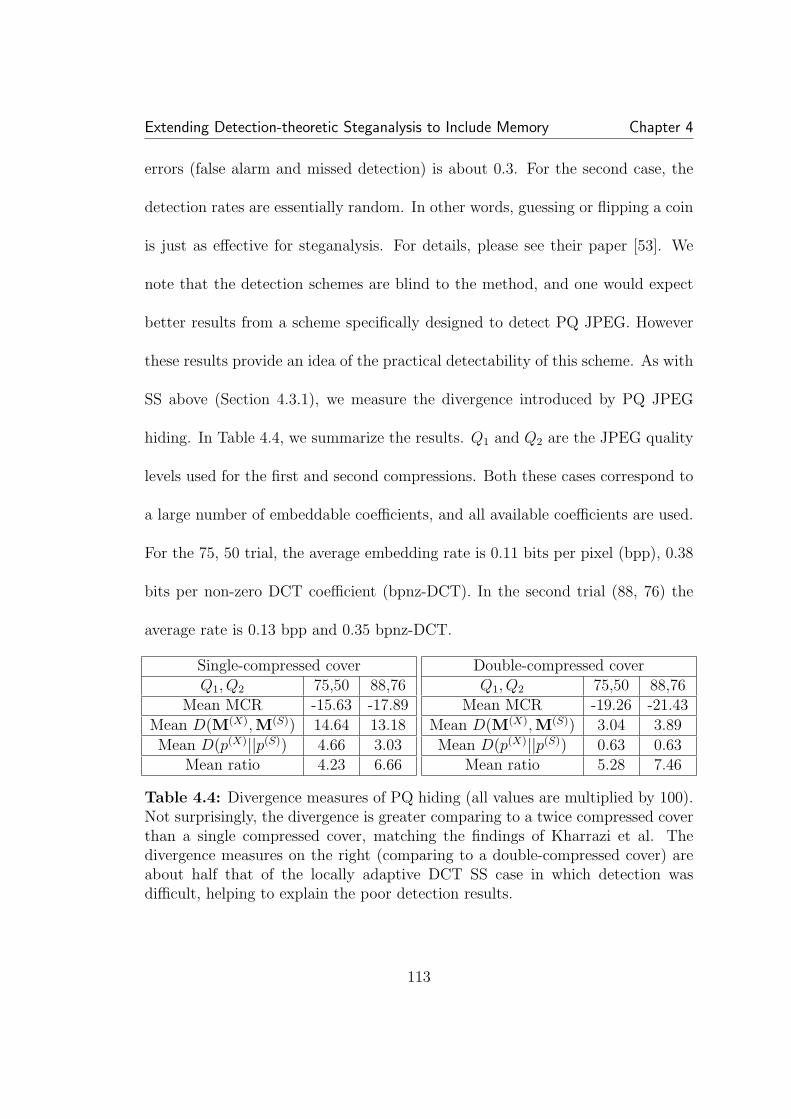
Extending Detection-theoretic Steganalysis to Include Memory Chapter 4
errors (false alarm and missed detection) is about 0.3. For the second case, the
detection rates are essentially random. In other words, guessing or flipping a coin
is just as effective for steganalysis. For details, please see their paper [53]. We
note that the detection schemes are blind to the method, and one would expect
better results from a scheme specifically designed to detect PQ JPEG. However
these results provide an idea of the practical detectability of this scheme. As with
SS above (Section 4.3.1), we measure the divergence introduced by PQ JPEG
hiding. In Table 4.4, we summarize the results. Q1 and Q2 are the JPEG quality
levels used for the first and second compressions. Both these cases correspond to
a large number of embeddable coefficients, and all available coefficients are used.
For the 75, 50 trial, the average embedding rate is 0.11 bits per pixel (bpp), 0.38
bits per non-zero DCT coefficient (bpnz-DCT). In the second trial (88, 76) the
average rate is 0.13 bpp and 0.35 bpnz-DCT.
Single-compressed coverQ1, Q2 75,50 88,76
Mean MCR -15.63 -17.89
Mean D(M(X),M(S)) 14.64 13.18
Mean D(p(X)||p(S)) 4.66 3.03Mean ratio 4.23 6.66
Double-compressed coverQ1, Q2 75,50 88,76
Mean MCR -19.26 -21.43
Mean D(M(X),M(S)) 3.04 3.89
Mean D(p(X)||p(S)) 0.63 0.63Mean ratio 5.28 7.46
Table 4.4: Divergence measures of PQ hiding (all values are multiplied by 100).Not surprisingly, the divergence is greater comparing to a twice compressed coverthan a single compressed cover, matching the findings of Kharrazi et al. Thedivergence measures on the right (comparing to a double-compressed cover) areabout half that of the locally adaptive DCT SS case in which detection wasdifficult, helping to explain the poor detection results.
113
Extending Detection-theoretic Steganalysis to Include Memory Chapter 4
As in the spread spectrum case, we found that the measure of theoretically
optimal detection of data hiding in Markov random chains corresponds to exper-
iments in the non-idealized case. This again suggests that the model is a useful
tool in judging the inherent detectability of a steganographic method. Addition-
ally there is a gain for a steganalyst to use dependency for detection, up to 7.5
times gain in this example. We now explore how this low divergence is obtained.
4.4.2 Statistical Model for Double JPEG Compressed PQ
As mentioned above, the source for data hiding is an image that has undergone
JPEG compression. During JPEG compression, the image is broken into small
blocks, each of which undergoes a 2-d discrete cosine transform (DCT). These
DCT coefficients are then quantized to reduce the number of bits used to store
or transmit the image (for details see [94]). An inverse DCT of these coefficients
reproduces a spatial domain image. However the spatial domain (pixel) values
are no longer integers, due to the quantization in the DCT domain. To display
or otherwise use the image in the spatial domain, the pixel values are rounded to
the nearest integer in the bit depth range (e.g. {0, 1, . . . , 255} for an 8-bit image).
Now the DCT coefficients (of the pixel image) are no longer exactly quantized,
but instead are randomly spread around the quantized value. So in summary,
if an image is compressed, then decompressed, the DCT values are randomly
114
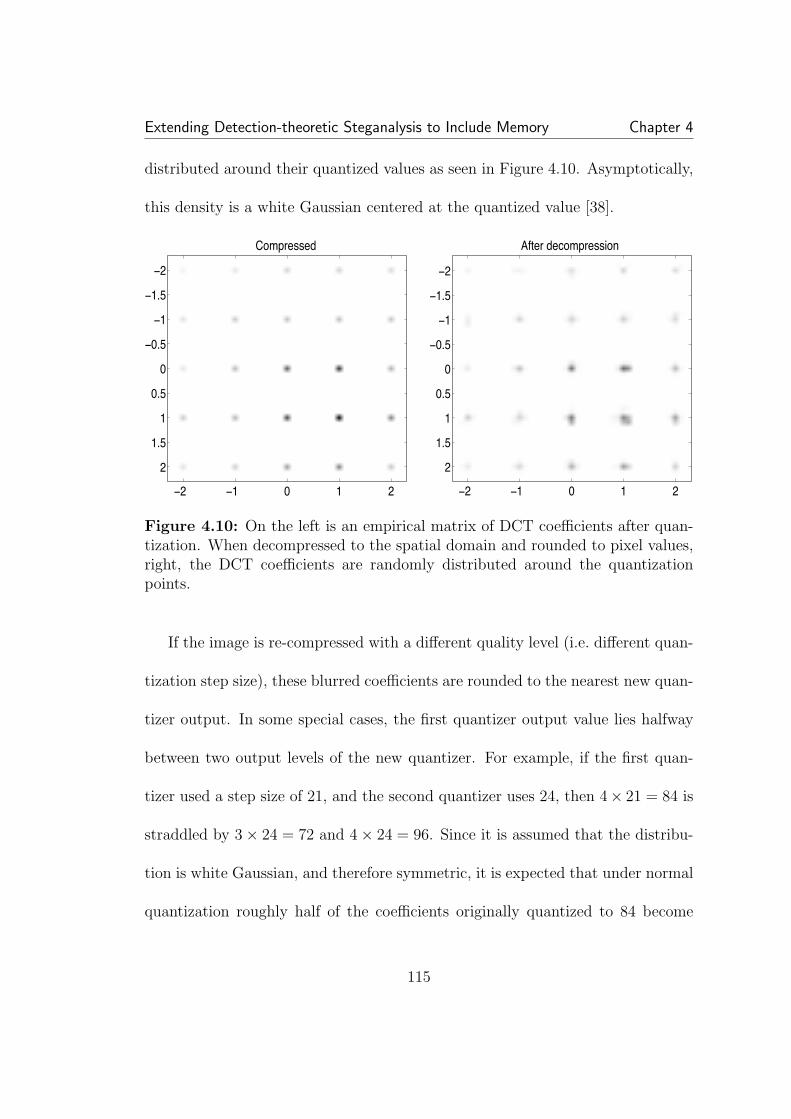
Extending Detection-theoretic Steganalysis to Include Memory Chapter 4
distributed around their quantized values as seen in Figure 4.10. Asymptotically,
this density is a white Gaussian centered at the quantized value [38].
Compressed
−2 −1 0 1 2
−2
−1.5
−1
−0.5
0
0.5
1
1.5
2
After decompression
−2 −1 0 1 2
−2
−1.5
−1
−0.5
0
0.5
1
1.5
2
Figure 4.10: On the left is an empirical matrix of DCT coefficients after quan-tization. When decompressed to the spatial domain and rounded to pixel values,right, the DCT coefficients are randomly distributed around the quantizationpoints.
If the image is re-compressed with a different quality level (i.e. different quan-
tization step size), these blurred coefficients are rounded to the nearest new quan-
tizer output. In some special cases, the first quantizer output value lies halfway
between two output levels of the new quantizer. For example, if the first quan-
tizer used a step size of 21, and the second quantizer uses 24, then 4× 21 = 84 is
straddled by 3× 24 = 72 and 4× 24 = 96. Since it is assumed that the distribu-
tion is white Gaussian, and therefore symmetric, it is expected that under normal
quantization roughly half of the coefficients originally quantized to 84 become
115
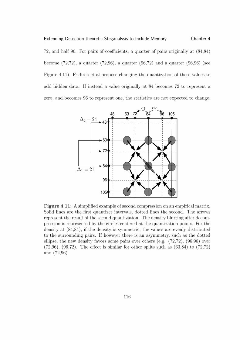
Extending Detection-theoretic Steganalysis to Include Memory Chapter 4
72, and half 96. For pairs of coefficients, a quarter of pairs originally at (84,84)
become (72,72), a quarter (72,96), a quarter (96,72) and a quarter (96,96) (see
Figure 4.11). Fridirch et al propose changing the quantization of these values to
add hidden data. If instead a value originally at 84 becomes 72 to represent a
zero, and becomes 96 to represent one, the statistics are not expected to change.
48
63
∆1 = 21
48
72
96
84
105
∆2 = 24
63 72 84 96 105-12 +12
Figure 4.11: A simplified example of second compression on an empirical matrix.Solid lines are the first quantizer intervals, dotted lines the second. The arrowsrepresent the result of the second quantization. The density blurring after decom-pression is represented by the circles centered at the quantization points. For thedensity at (84,84), if the density is symmetric, the values are evenly distributedto the surrounding pairs. If however there is an asymmetry, such as the dottedellipse, the new density favors some pairs over others (e.g. (72,72), (96,96) over(72,96), (96,72). The effect is similar for other splits such as (63,84) to (72,72)and (72,96).
116
Extending Detection-theoretic Steganalysis to Include Memory Chapter 4
This statistical equivalency only fails if the density blurring is not, in fact,
symmetric about the original quantization point. Though asymptotically it is
expected to be, each realization is slightly asymmetric, as can be seen in Figure
4.10. We have found the asymmetry to be small, however the calculated diver-
gence between a double compressed cover image and a PQ stego image is expected
to be greater than zero. The net effect however is minimal and the divergence
and detection results above are not surprising. Again we see a match between
analysis, divergence measurements, and practical detection.
4.5 Outguess
Outguess is a data hiding tool designed to hide in the least significant bits of
JPEG coefficients. Outguess 0.2 [68] is an improved version in which some of the
coefficients are used for hiding, while the rest are used to restore the histogram
to the cover state. Naturally this will prevent detection by histogram based
techniques such as the chi-squared and approximate LLRT methods explored in
Section 3.2. However it is shown by Fridrich et al [34] that although the histogram
of DCT coefficients is compensated, the dependencies in the spatial domain will
be changed. Specifically, the disruption at the boundaries of the 8 by 8 JPEG
blocks is greater for Outguess hiding than for standard JPEG compression. We
117
Extending Detection-theoretic Steganalysis to Include Memory Chapter 4
note in Section 4.2.2 that the blockiness statistic used to measure this disruption
is a function of the empirical matrix of the values straddling the JPEG blocks. A
key component of detection done by Fridrich et al using the blockiness measure is
a method of calibrating the statistic for each image, that is, a means a estimating
the cover blockiness. They use a method designed for blockwise transform hiding
schemes to do this. An estimate of the cover image is made by cropping the image
under scrutiny by half the size of a JPEG block and re-compressing. From this
estimated cover image, an estimate of the original blockiness is easy to compute.
We examine the detection of Outguess using the supervised learning detector
exploiting spatial dependencies we use to detect spread spectrum hiding. That is,
like Fridrich et al, we use spatial dependencies to detect Outguess. However we do
not calibrate on a per image basis, but instead train on hundreds of examples. In
Figure 4.12 we present results on various classifiers detecting Outguess in images.
The feature vector is built similar to those used in Section 4.3.3 to detect spread
spectrum hiding. To capture the block boundary dependency changes, vertical
and horizontal dependencies are included in the feature. Detection here, as re-
flected in the ROC, is not particularly powerful. This demonstrates the benefit
of using auto-calibration on an image-by-image basis. However such methods are
not always available, and a possible solution for the steganographer is to simply
use different block sizes.
118
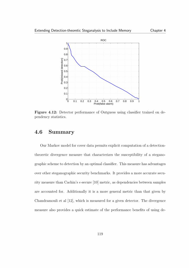
Extending Detection-theoretic Steganalysis to Include Memory Chapter 4
0 0.1 0.2 0.3 0.4 0.5 0.6 0.7 0.8 0.9 10
0.1
0.2
0.3
0.4
0.5
0.6
0.7
0.8
0.9
1ROC
Prob(false alarm)
Pro
b(m
isse
d de
tect
ion)
Figure 4.12: Detector performance of Outguess using classifier trained on de-pendency statistics.
4.6 Summary
Our Markov model for cover data permits explicit computation of a detection-
theoretic divergence measure that characterizes the susceptibility of a stegano-
graphic scheme to detection by an optimal classifier. This measure has advantages
over other steganographic security benchmarks. It provides a more accurate secu-
rity measure than Cachin’s ε-secure [10] metric, as dependencies between samples
are accounted for. Additionally it is a more general metric than that given by
Chandramouli et al [12], which is measured for a given detector. The divergence
measure also provides a quick estimate of the performance benefits of using de-
119
Extending Detection-theoretic Steganalysis to Include Memory Chapter 4
pendency in steganalysis: the ratio of the divergence for the Markov model, to
the divergence between marginal PMFs, represents the factor by which the use
of dependency reduces the number of samples required for a given performance,
relative to steganalysis based on one-dimensional histograms.
While the Markov model does not completely capture interpixel dependen-
cies in images, we have shown it to be consistent with many image steganaly-
sis schemes exploiting memory, which typically use a function of the statistics
used to optimally discriminate between Markov source models. Furthermore, the
detection-theoretic benchmarks computed using the Markov model are close to
the performance attained by practical image steganalysis techniques. However,
further research is needed into whether more complex statistical models can yield
better image steganalysis techniques, and how to compute performance bench-
marks for such techniques.
Improved models for images could include more degrees of dependency, as
well as some model of non- or piecewise-stationarity. Recently we have seen work
extend the i.i.d. approach to LSB analysis by employing models with memory:
Draper et al [23] generalize our approach by considering adjacent pixel dependen-
cides and Sidorov has performed hidden Markov model (HMM) analysis [78] on
LSB hiding and used a MC derived statistic for LSB detection [79, in Russian].
Draper et al concluded that adding one level of dependency (i.e. considering two-
120
Extending Detection-theoretic Steganalysis to Include Memory Chapter 4
dimensional joint statistics) provided diminishing marginal returns. They observe
that detectors employing a non-PMF statistic, such as RS analysis [33], perform
very well, and consider PMFs an inferior tool for practical steganalysis. We stress
that PMF analysis provides bounds on optimal detection, however these bounds
are for the asymptotic case. Their observations are for finite a number of samples,
an important consideration in comparing optimal detection to practical schemes.
Sidorov found that considering one level of dependency (MC model) only showed
good results for high-quality and synthetic images; for low-quality images the de-
tector failed. In the related paper [78] the author considers extending the MC
model to a Markov random field model, incorporating a higher degree of depen-
dency, but does not implement such a detector. We note that the parameters of
more complex models are more difficult to estimate for finite number of samples, a
well-known problem [15]. Additionally variations from image to image may make
it difficult to calibrate steganalysis techniques based on such models.
The Markov chain model can be related to Sallee’s [75] model based approach.
Rather than assuming the steganalyst is limited to a parameterized distribution
model, we assume the actual joint distribution is used. Just as with Sallee’s
steganography, the security is only as good as the model. Thus, much work re-
mains to be done on the fundamental problem of understanding how the complex-
ity of the model for the cover data impacts the accuracy of estimating the model
121

Extending Detection-theoretic Steganalysis to Include Memory Chapter 4
parameters, and the computational complexity and performance of steganalysis
based on the model.
122
Chapter 5
Evading Optimal StatisticalSteganalysis
We now turn our attention to applying our detection-theoretic framework
to prevent detection. In particular we seek to find methods that maintain an
adequate rate, and can withstand at least nominal interference between sender and
receiver, for example from an active warden, transmission noise, or compression.
We note many previous methods designed to reduce detectability (outlined in
Chapter 2) have focused on a particular steganalysis statistic. We know from
our study of steganalysis that for perfectly secure embedding, the distribution of
the stego data must exactly match the cover, which we have seen does not occur
by default. Other methods such as stochastic modulation [31], JPEG perturbed
quantization [38], and model based embedding [75, 76] accept a change of stego
distribution from the original cover, but attempt to match a different distribution,
which is close to a plausible cover distribution. It is difficult to define what is
123

Evading Optimal Statistical Steganalysis Chapter 5
“plausible enough”, and in some cases (e.g. [7]) a steganalyst can exploit the
divergence from the original. Additionally, these approaches are very fragile to
any interference between sender and receiver.
Provos’ Outguess [68] is an early attempt at restoring the stego distribution
to the cover empirical distribution. This method was followed up later by Eggers
et al [26], with a more mathematical formulation denoted histogram-preserving
data mapping (HPDM), and Franz, with work in matching the message data to
the cover distribution [29]. All of these schemes are designed for compensat-
ing discrete-valued hiding medium. Theoretical proposals for continuous-valued
hiding compensation have also been presented. In [43] Guillon et al suggest trans-
forming the cover samples before hiding, such that the cover samples are uniformly
distributed. QIM hiding in uniformly distributed data does not change the dis-
tribution. It is likely however that robustness would suffer with such a scheme,
and it may be difficult to implement in practice. Wang and Moulin [98] proposed
stochastic QIM, which achieves zero K-L divergence. Because of the random
nature of the hiding, it is difficult to judge the robustness of stochastic QIM.
124
Evading Optimal Statistical Steganalysis Chapter 5
5.1 Statistical Restoration Scheme
As with our study of steganalysis, we begin with an i.i.d. assumption and later
extend this to a Markov chain model. Under the independence assumption, our
goal for perfect security is to match the marginal distribution. In practice, the
underlying distribution of an image is not known. Our approach then is to match
the empirical distribution of the image. Since the empirical distribution is derived
from a cover image, there is no doubt it is a plausible cover distribution. The
plan is to save coefficients otherwise used for embedding to instead compensate
the distribution, similar to Provos’ [68] method to restore the histogram of JPEG
coefficients. The goal here however is to recover a continuous distribution, the pdf,
rather than the PMF. In this way, hiding media such as DCT coefficients which
have not been quantized can be statistically compensated. Naturally, if these
coefficients are later quantized, they will still match the expected distribution of
the quantized cover.
Practically speaking, the steganalyst does not have access to continuous pdfs,
but instead calculates a histogram approximation. Our data hiding is secure if
we match the stego histogram to the cover histogram using a bin size, denoted
w, the same size as, or smaller than, that employed by the steganalyst. We
stress that all values are present and there are no “gaps” in the distribution of
125
Evading Optimal Statistical Steganalysis Chapter 5
values; however, within each bin the data is matched to the bin center. A key
assumption is that for small enough w, the distribution is uniformly distributed
over the bin, a common assumption in source coding [40]. Under this assumption,
we can generate uniformly distributed pseudorandom (PR) data to cover each bin,
and still match the original statistics. Let fX(x) be the cover probability density
function (pdf) and fS(s) the stego pdf. For I bins centered at t[i], i ∈ [1, I] with
constant width w, the expected histogram for data generated from fX(x) is:
PEX [i] =
∫ t[i]+w/2
t[i]−w/2
fX(x)dx (5.1)
with a similar derivation of PES [i] from fS(s). The superscript E denotes that this
is the expected histogram, to discriminate it from histograms calculated from ran-
dom realizations. We generally refer to these expected quantized pdfs as PMFs.
The hiding scheme we analyze here is outlined in greater detail in [81]. The
key points we need for our analysis are as follows:
• A proportion of coefficients are used for hiding, the rest are used for com-
pensating the distribution after hiding.
• The compensating coefficients are uniformly (PR) distributed within the
bins, so there are no gaps in the pdf. In our QIM implementation this is
accomplished with dithered quantization.
126
Evading Optimal Statistical Steganalysis Chapter 5
• A minimum mean squared error (MMSE) criteria is used to minimize dis-
tortion while hiding
Let λ ∈ [0, 1) be the ratio of symbols used for hiding, so 1 − λ is the ratio
remaining to match the cover histogram. If PX [i] is the cover histogram, PS[i]
the standard (uncompensated) stego histogram, PC [i] the histogram of compen-
sating coefficients, and PZ [i] the histogram of the final output, our goal can be
summarized as:
PZ [i] = PX [i] ∀ i
PZ [i] , λPS[i] + (1− λ)PC [i]
(5.2)
We first examine the effect of allowing a small, low probability region to remain
uncompensated after hiding. By ignoring these regions, the rate can be increased
significantly. However since the distribution is not perfectly matched, there is
a measurable K-L divergence between the cover and stego pdfs. We study this
tradeoff between divergence and rate, and find, not surprisingly, that restoration
effects a more efficient tradeoff than simply embedding in fewer coefficients. We
then focus on eliminating all divergence, and derive an expression for the expected
rate with a given cover distribution. Finally we expand this analysis to statistical
restoration of the joint histogram, or empirical matrix.
127

Evading Optimal Statistical Steganalysis Chapter 5
5.2 Rate Versus Security
Using a set of embedding coefficients for compensating instead of hiding re-
duces the size of the message that can be hidden; this is the cost of increasing
security. We can characterize this cost by studying the amount of data that can
be hidden in an idealized data source with a given distribution.
The amount of data that can be hidden is proportional to the number of sym-
bols that can be hidden in. So to maximize the amount of data we send, we seek
to maximize λ for a given cover histogram subject to the constraint in (5.2), and
the constraints imposed on the distribution of compensating coefficients, namely∑PC [i] = 1 and PC [i] ≥ 0 ∀ i. The first constraint is true for all λ. For the
second constraint, by substituting an expression for PC satisfying (5.2), we find:
PC [i] ≥ 0 ∀ i
PX [i]− λPS[i]
(1− λ)≥ 0
−λPS[i] ≥ −PX [i]
λ ≤ PX [i]
PS[i]∀ i
which gives us an upper limit on the percentage of symbols we can use for hiding.
Ideally the sender would use a different λ for each bin. However hiding shifts
values from one bin to another, and the valid λ for one bin may be larger than
an adjacent bin and the constraint is violated. Because of this, a worst-case λ is
128
Evading Optimal Statistical Steganalysis Chapter 5
chosen:
λ∗ , mini
PX [i]
PS[i]
However if we apply this constraint on λ to typical PMFs we run into erratic
behavior in the low-probability tails. The ratio PX [i]PS [i]
can vary widely here, from
infinitesimally small to quite large. This is because the magnitude of changes to
the ratio depends on the value of PX [i], for example: 0.500.49
is very close to 0.500.51
whereas 0.020.01
is quite different from 0.020.03
. We study this phenomenon in greater
detail in Section 5.3. We note however that since the probabilities of the corre-
sponding events are low, then the effect of PMF differences in these regions on the
net divergence is small. So to avoid this problem we can relax the exact equality
constraint and not require compensation in a small, low probability region of the
PMF. In the next section, we focus on achieving perfect matching for the entire
PMF. With the relaxed constraint:
λ∗ = mini∈C
PX(i)
PS(i)
where C is the compensated region. In addition to the divergence introduced
to the ignored (Cc) region, since (5.2) is no longer true for all i, PC must be
normalized to satisfy the unity sum constraint, adding a small change across the
PMF. Though the net effect is to introduce a small amount of divergence, λ and
the corresponding hiding rate can only increase. A tradeoff can be made between
129

Evading Optimal Statistical Steganalysis Chapter 5
desired security from detection and the hiding rate. We note that another method
to increase security at the cost of embedding payload is to simply embed in fewer
coefficients. However we expect that explicitly fixing the histogram with the
remaining coefficients has a greater effect at reducing divergence. We verify this
assumption for a specific scheme outlined below.
To gauge the effect of hiding in practice, we examine the compensation scheme
adapted to QIM hiding with dithering (see Section 3.3). We examine the hiding ef-
fect on covers with Gaussian and Laplacian distributions with different variances.
Additionally we change hiding parameters such as the step size of the hiding quan-
tizer, ∆. As expected from our findings on QIM steganalysis, we found the rate
and divergence to be related to the ratio σ/∆ within a given PMF family. For
our tests comparing rate and divergence, we would then expect different tradeoffs
for different cover distributions and different σ/∆.
To find the rate-divergence tradeoff, we find the rate corresponding to several
different sizes of ignored (uncompensated) regions. A larger ignored region has a
greater divergence from the original, but eliminates small PX [i]PS [i]
, which increases
λ, the hiding rate. This tradeoff for restoration is compared to the tradeoff for
simply embedding less. In Figure 5.1 we see a large decrease in divergence can be
made with a small drop in rate, which is not possible by merely embedding less.
This is true for both Laplacian and Gaussian PMFs over a range of σ/∆.
130
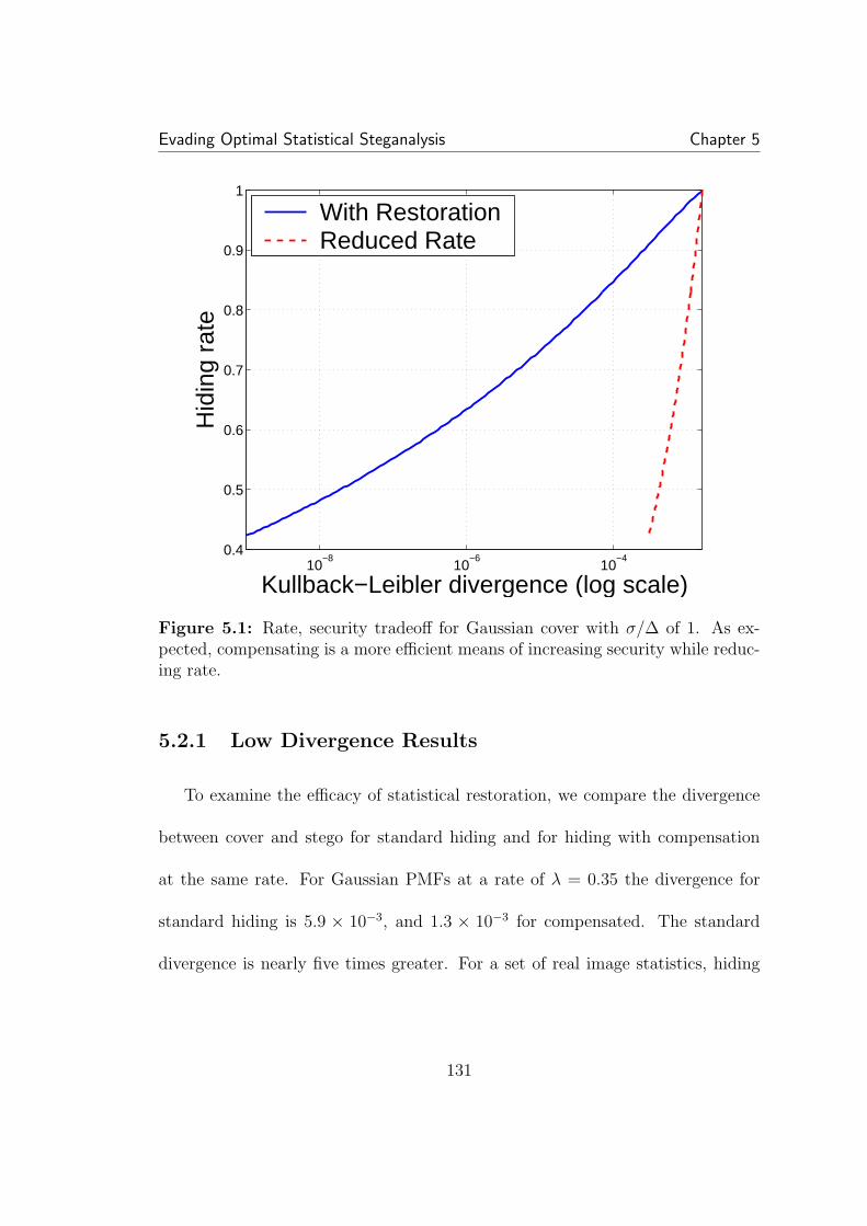
Evading Optimal Statistical Steganalysis Chapter 5
10−8
10−6
10−4
0.4
0.5
0.6
0.7
0.8
0.9
1
Kullback−Leibler divergence (log scale)
Hid
ing
rate
With RestorationReduced Rate
Figure 5.1: Rate, security tradeoff for Gaussian cover with σ/∆ of 1. As ex-pected, compensating is a more efficient means of increasing security while reduc-ing rate.
5.2.1 Low Divergence Results
To examine the efficacy of statistical restoration, we compare the divergence
between cover and stego for standard hiding and for hiding with compensation
at the same rate. For Gaussian PMFs at a rate of λ = 0.35 the divergence for
standard hiding is 5.9 × 10⁻³, and 1.3 × 10⁻³ for compensated. The standard
divergence is nearly five times greater. For a set of real image statistics, hiding
131
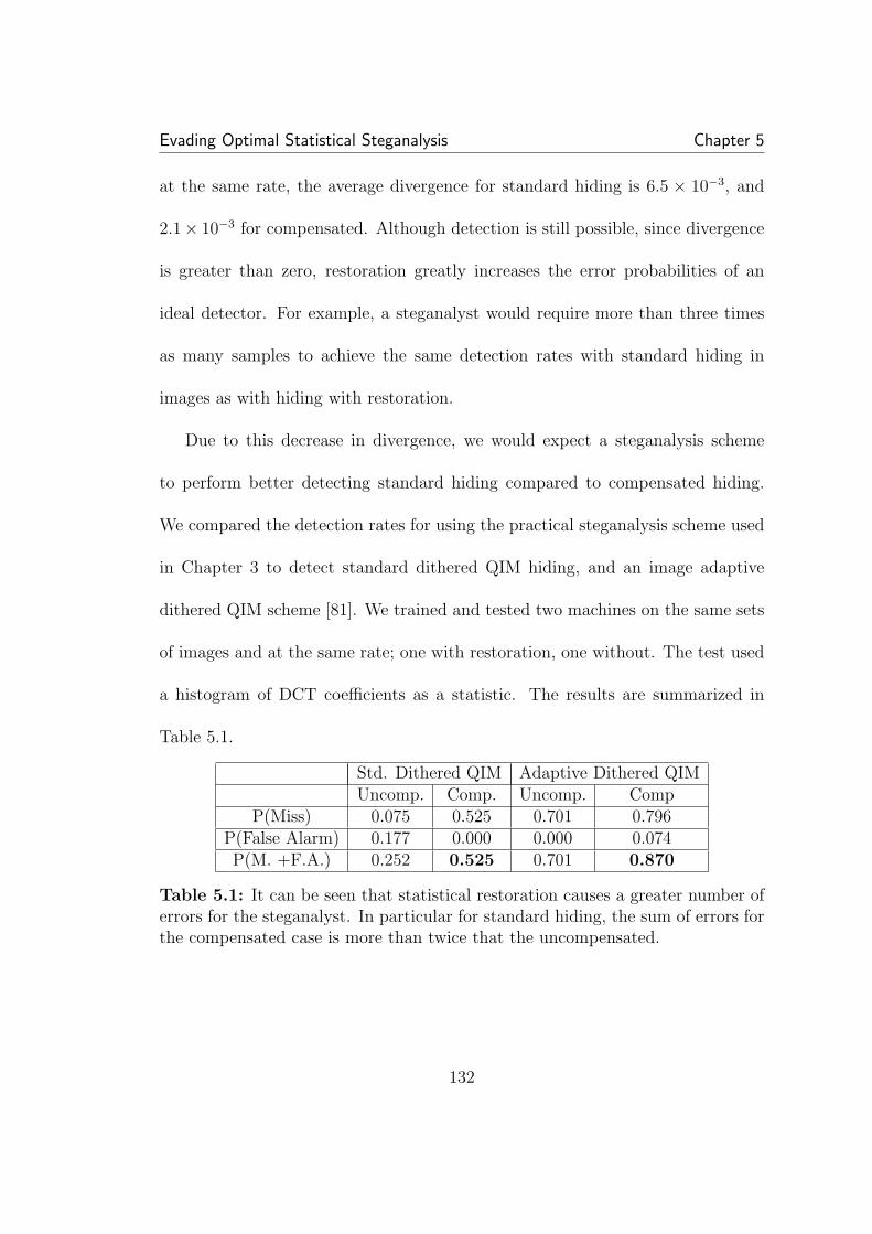
Evading Optimal Statistical Steganalysis Chapter 5
at the same rate, the average divergence for standard hiding is 6.5 × 10⁻³, and
2.1× 10⁻³ for compensated. Although detection is still possible, since divergence
is greater than zero, restoration greatly increases the error probabilities of an
ideal detector. For example, a steganalyst would require more than three times
as many samples to achieve the same detection rates with standard hiding in
images as with hiding with restoration.
Due to this decrease in divergence, we would expect a steganalysis scheme
to perform better detecting standard hiding compared to compensated hiding.
We compared the detection rates for using the practical steganalysis scheme used
in Chapter 3 to detect standard dithered QIM hiding, and an image adaptive
dithered QIM scheme [81]. We trained and tested two machines on the same sets
of images and at the same rate; one with restoration, one without. The test used
a histogram of DCT coefficients as a statistic. The results are summarized in
Table 5.1.
Std. Dithered QIM Adaptive Dithered QIMUncomp. Comp. Uncomp. Comp
P(Miss) 0.075 0.525 0.701 0.796P(False Alarm) 0.177 0.000 0.000 0.074P(M. +F.A.) 0.252 0.525 0.701 0.870
Table 5.1: It can be seen that statistical restoration causes a greater number oferrors for the steganalyst. In particular for standard hiding, the sum of errors forthe compensated case is more than twice that the uncompensated.
132

Evading Optimal Statistical Steganalysis Chapter 5
We have found that detection rates are decreased, but are still better than
random guessing, which is expected due to the allowed difference between cover
and stego distributions. We now examine zero divergence hiding and rate.
5.3 Hiding Rate for Zero K-L Divergence
We here analyze the proposed solution for perfect restoration and characterize
the maximum message size that can be hidden. In particular, by finding the dis-
tribution of the rate allowing perfect restoration, we can find a rate guaranteeing
zero divergence within a given probability threshold. Though the approach we
use can be applied to statistical restoration of any hiding scheme, we show the
specific example of our QIM scheme.
5.3.1 Rate Distribution Derivation
We now examine an approach where no region is left uncompensated, and
so the histogram can be perfectly matched. To do this, we need to find the
distribution of the minimum of the histogram ratio, λ∗ for a given cover pdf,
fX(x). We note that histograms calculated from real data {Xn}N1 vary for each
realization. In other words, the number of symbols in the bins, NPX [i], are
random variables. Be analyzing the distribution of these random variables, we
133

Evading Optimal Statistical Steganalysis Chapter 5
can find the distribution of the ratio PX [i]PS [i]
for each bin, and from this the statistics
of λ∗. We point out that the density of a ratio is not equal to the ratio of the
density, that is, in general
f
(PX [i]
PS[i]
)6= f(PX [i])
f(PS[i])
Let VX [i] = NPX [i] be the number of symbols from fX(x) falling into bin i,
then VX [i] has binomial density function PVX [i] = B{N, PEX [i]} [77]. Similarly if
VS[i] is the number of symbols per bin for data from fS(s), it is distributed as
B{N, PES [i]}. See Figure 5.2 for a schematic of finding the distribution of the bins
of a histogram.
We now define Γ[i] , VX [i]VS [i]
= PX [i]PS [i]
. The cumulative distribution of Γ[i],
FΓ[i](γ) = P (Γ[i] ≤ γ), is given by
FΓ[i](γ) =N∑
k=0
bγkc∑l=0
PVS [i](k)PVX [i](l)
and the density is
fΓ[i](γ) =dFΓ[i](γ)
dγ.
Ultimately, we wish to find the distribution of the minimum Γ over all bins,
giving us a statistical description of λ∗, our zero-divergence hiding rate. The
cumulative distribution of λ∗ is the distribution of mini Γ[i] given by
Fλ∗(γ) = 1−
{∏i
[1− FΓ[i](γ)
]}
134
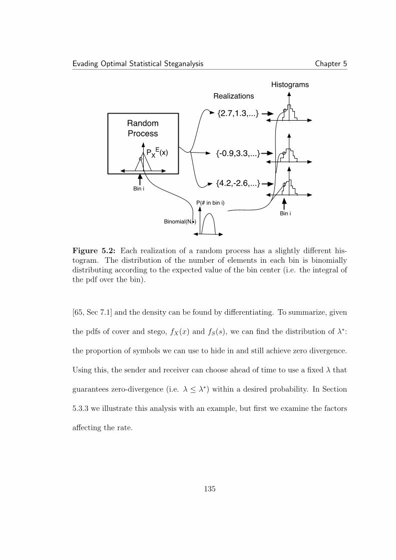
Evading Optimal Statistical Steganalysis Chapter 5
Histograms
RandomProcess
PXE(x)
{2.7,1.3,...}
{-0.9,3.3,...}
{4.2,-2.6,...}
Realizations
Bin iBinomial(N, )
Bin i
P(# in bin i)
Figure 5.2: Each realization of a random process has a slightly different his-togram. The distribution of the number of elements in each bin is binomiallydistributing according to the expected value of the bin center (i.e. the integral ofthe pdf over the bin).
[65, Sec 7.1] and the density can be found by differentiating. To summarize, given
the pdfs of cover and stego, fX(x) and fS(s), we can find the distribution of λ∗:
the proportion of symbols we can use to hide in and still achieve zero divergence.
Using this, the sender and receiver can choose ahead of time to use a fixed λ that
guarantees zero-divergence (i.e. λ ≤ λ∗) within a desired probability. In Section
5.3.3 we illustrate this analysis with an example, but first we examine the factors
affecting the rate.
135

Evading Optimal Statistical Steganalysis Chapter 5
5.3.2 General Factors Affecting the Hiding Rate
By examining the derivation of the distribution of λ∗, we can predict the effect
of various parameters on the hiding rate. The key factors effecting the payload
are:
1. Cover and stego pdfs, fX , fS: Obviously the “closer” the two pdfs are
to one another, the less compensation is required, and the higher the rate.
The difference between the pdfs generally depends on the hiding scheme.
2. Number of samples, N : The greater the number of samples, the more
accurate our estimates of the samples per bin. Therefore it is easier to
guarantee a λ to be safe with given probability, and so the hiding rate is
higher. The number of samples is mostly a function of the size of the image.
3. Bin width, w, used for compensation: Bin width is important to guar-
anteeing security, but the effect of bin width is not immediately clear, and
is a research topic in its own right [77, 95]. We briefly explore the net effect
of w on λ∗ below.
To judge the effect of w, we examine the expected value of Γ, the ratio of PX
to PS. To avoid problems with dividing by zero we instead use Γ′ , min(Γ, 1).
Since Γ greater than one implies embedding at greater than 100%, these cases can
be ignored. From (5.1) we note that a smaller bin width leads to smaller expected
136
Evading Optimal Statistical Steganalysis Chapter 5
bin values, PEX [i] and PE
S [i]. By evaluating
E{Γ′} =N∑
k=0
n∑l=0
min
(l
k, 1
)PVS [i](k)PVX [i](l)
for several distributions PVS [i], PVX [i] (recall these are binomially distributed based
on PES , PE
X ), we find that for a set ratio of expected bin values, PEX [i]/PE
S [i],
the expected value of Γ′ increases as PES and PE
X decrease. In other words, the
expected value of Γ′ increases as the bin width decreases. This is particularly
true for small PEX (and therefore small Γ′). For larger PE
X (greater than 0.1) the
expected value of the ratio is basically equal to the ratio of the expected value for
any bin size. Additionally, the variance of Γ′ (evaluated in the same manner as
the mean) decreases as PES and PE
X decrease. Both of these trends would indicate
that decreasing w increases the hiding rate. However this only accounts for a
reduction of bin width for a fixed bin center. As w decreases, new bins must be
created. λ∗, is evaluated as the minimum over all the bins. Intuitively, as the
number of bins increases there is an increased probability of a smaller minimum.
So the net effect, an increase or decrease in E{λ∗}, depends on the distribu-
tions. We then must evaluate the net effect of bin width on λ∗ for given cover and
stego pdfs. Fortunately for the steganographer, the steganalyst can not choose an
arbitrarily small bin size in order to detect, as the mean integrated square error
(MISE) of the detector’s estimate of the pdf is not simply inversely related to bin
width [77]. In other words, the detector also faces a challenge in choosing an ap-
137

Evading Optimal Statistical Steganalysis Chapter 5
propriate bin size. Empirically, both the steganographer and steganalyst should
try to use as large a bin width as possible, while still maintaining the uniform
approximation over each bin.
5.3.3 Maximum Rate of Perfect Restoration QIM
We now apply the findings of the previous section to the case of quantization
index modulation (QIM) data hiding, specifically dithered uniform scalar QIM
[14]. For a given cover pdf fX(x) we know the expected pdf for data after un-
dergoing dithered scalar QIM with constant step-size ∆ from our steganalysis of
QIM (Section 3.3):
fS(s) =1
∆
∫ s+∆/2
s−∆/2
fX(x)dx ≡[fX(x) ∗ 1
∆u (x/∆)
](s)
where u(t) is the rectangle function, defined in terms of the unit step function
u(t) as u(t) = u(t + 1/2) − u(t − 1/2). As we found in Section 3.3, without
compensation, this change can be detected when hiding in real images. We now
show how to find λ∗ allowing for perfect histogram restoration of QIM hiding.
Earlier we listed general factors affecting the amount of data that can be
embedded while allowing histogram compensation. In the context of QIM hiding
we can more explicitly characterize these factors. Since we can calculate fS from
fX , of this pair we need only examine the cover pdf. Since fS is a smoothed
138
Evading Optimal Statistical Steganalysis Chapter 5
version of fX (after convolution), the ideal fX for secure QIM hiding is uniform
[43], which can not be smoothed any further. Unfortunately it is difficult to
find a uniformly distributed cover medium. Typical hiding medium, particularly
transform domain coefficients, are sharply peaked. As noted earlier, σ/∆ is an
important parameter for QIM. For large σ/∆, the cover pdf is flat relative to
the quantization interval, and less change is caused to the original histogram
by hiding. Therefore less samples are needed for compensation, and more are
available for hiding, and the expected λ∗ is large. Conversely a small σ/∆ has a
low expected λ∗.
Of all the factors, only w and ∆ are in the hands of the steganographer. De-
creasing ∆ increases σ/∆, and therefore the safe hiding rate. However, decreasing
∆ also increases the chance of decoding error due to any noise or attacks [14].
Thus if a given robustness is required, ∆ can also be thought of as fixed, leaving
only the bin width. For QIM hiding in Gaussians and Laplacians, we found that
decreasing the bin size w led to a decrease in λ∗, suggesting that the stegano-
grapher should choose a large w. However, as mentioned before, w should be
chosen carefully to avoid detection by a steganalyst using a smaller w.
We presently examine an idealized QIM scheme, followed by an extension to
our practical QIM scheme which prevents decoder errors. As an illustrative ex-
139
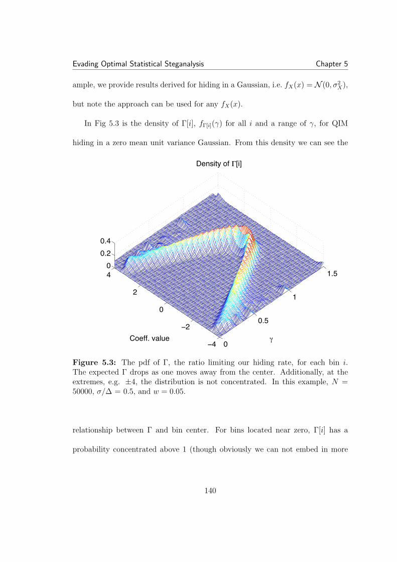
Evading Optimal Statistical Steganalysis Chapter 5
ample, we provide results derived for hiding in a Gaussian, i.e. fX(x) = N (0, σ2X),
but note the approach can be used for any fX(x).
In Fig 5.3 is the density of Γ[i], fΓ[i](γ) for all i and a range of γ, for QIM
hiding in a zero mean unit variance Gaussian. From this density we can see the
0
0.5
1
1.5
−4
−2
0
2
40
0.2
0.4
γ
Density of Γ[i]
Coeff. value
Figure 5.3: The pdf of Γ, the ratio limiting our hiding rate, for each bin i.The expected Γ drops as one moves away from the center. Additionally, at theextremes, e.g. ±4, the distribution is not concentrated. In this example, N =50000, σ/∆ = 0.5, and w = 0.05.
relationship between Γ and bin center. For bins located near zero, Γ[i] has a
probability concentrated above 1 (though obviously we can not embed in more
140
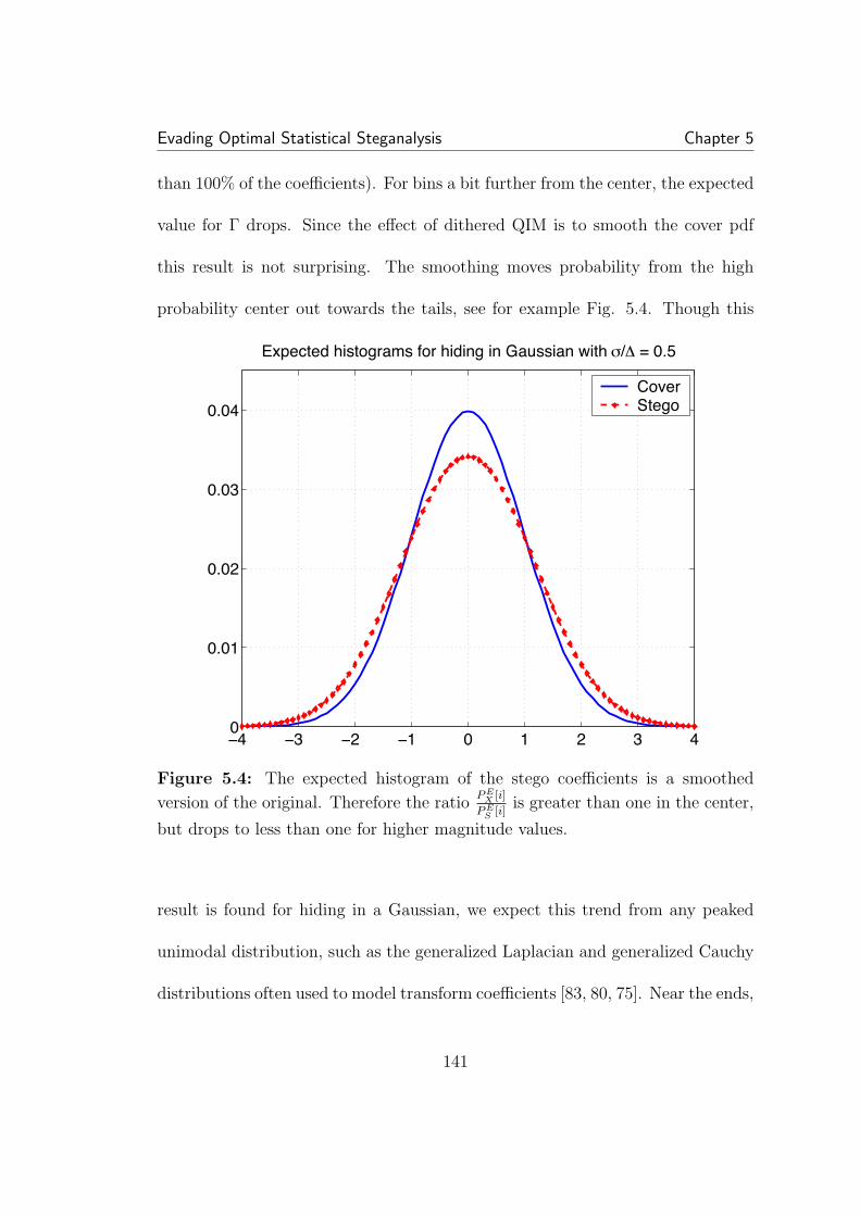
Evading Optimal Statistical Steganalysis Chapter 5
than 100% of the coefficients). For bins a bit further from the center, the expected
value for Γ drops. Since the effect of dithered QIM is to smooth the cover pdf
this result is not surprising. The smoothing moves probability from the high
probability center out towards the tails, see for example Fig. 5.4. Though this
−4 −3 −2 −1 0 1 2 3 40
0.01
0.02
0.03
0.04
Expected histograms for hiding in Gaussian with σ/∆ = 0.5
CoverStego
Figure 5.4: The expected histogram of the stego coefficients is a smoothed
version of the original. Therefore the ratioP E
X [i]
P ES [i]
is greater than one in the center,
but drops to less than one for higher magnitude values.
result is found for hiding in a Gaussian, we expect this trend from any peaked
unimodal distribution, such as the generalized Laplacian and generalized Cauchy
distributions often used to model transform coefficients [83, 80, 75]. Near the ends,
141

Evading Optimal Statistical Steganalysis Chapter 5
e.g. ±4, Γ is distributed widely over all possible values. So while it is possible
to have a very high γ here, it is also possible to be very low; i.e. the variance is
very high. We empirically observed these problems in the low probability tails
in Section 5.2. The first solution proposed is to hide in all coefficients but only
compensate bins away from these tails. We now attempt to only hide in the
high probability region; after hiding, only this region needs to be compensated.
This introduces a practical problem, the decoder is not always able to distinguish
between embedded coefficients and non-embedded. We address this issue below,
but first we examine the ideal case. So our motivation is, even though we must
reduce the number of embeddable coefficients by not embedding in high valued,
low probability coefficients, our net rate may be higher due to a higher λ∗, where
λ∗ is redefined as
λ∗ , mini∈H
PX [i]
PS[i]
where H is the hiding region, defined as H , [−T, T ] where T is a threshold.
The net hiding rate, no longer simply equivalent to λ∗, is now
R = λ∗G(H)
where
G(H) ,∑i∈H
PX [i].
142
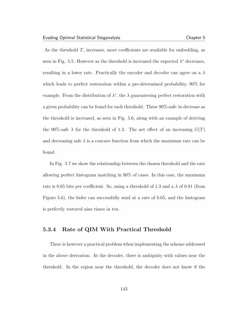
Evading Optimal Statistical Steganalysis Chapter 5
As the threshold T , increases, more coefficients are available for embedding, as
seen in Fig. 5.5. However as the threshold is increased the expected λ∗ decreases,
resulting in a lower rate. Practically the encoder and decoder can agree on a λ
which leads to perfect restoration within a pre-determined probability, 90% for
example. From the distribution of λ∗, the λ guaranteeing perfect restoration with
a given probability can be found for each threshold. These 90%-safe λs decrease as
the threshold is increased, as seen in Fig. 5.6, along with an example of deriving
the 90%-safe λ for the threshold of 1.3. The net effect of an increasing G(T )
and decreasing safe λ is a concave function from which the maximum rate can be
found.
In Fig. 5.7 we show the relationship between the chosen threshold and the rate
allowing perfect histogram matching in 90% of cases. In this case, the maximum
rate is 0.65 bits per coefficient. So, using a threshold of 1.3 and a λ of 0.81 (from
Figure 5.6), the hider can successfully send at a rate of 0.65, and the histogram
is perfectly restored nine times in ten.
5.3.4 Rate of QIM With Practical Threshold
There is however a practical problem when implementing the scheme addressed
in the above derivation. At the decoder, there is ambiguity with values near the
threshold. In the region near the threshold, the decoder does not know if the
143
Evading Optimal Statistical Steganalysis Chapter 5
0.5 1 1.31.5 2 2.5 3 3.5 40
0.1
0.2
0.3
0.4
0.5
0.6
0.7
0.8
0.9
1Threshold vs. Percentage of Available Coefficients
Threshold
G(T
)
Figure 5.5: A larger threshold allows a greater number of coefficients to beembedded. This partially offsets the decrease in expected λ∗ with increasedthreshold.
received value is a coefficient that originally was below the threshold and is now
shifted above the threshold after hiding and dithering, or is simply a coefficient
that originally was above the threshold and contains no data. Therefore we create
a buffer zone near the threshold: if, after hiding, a coefficient would be shifted
above the threshold, it is instead skipped over. To prevent creating an abrupt
transition in the histogram at the buffer zone, we dither the threshold with the
144
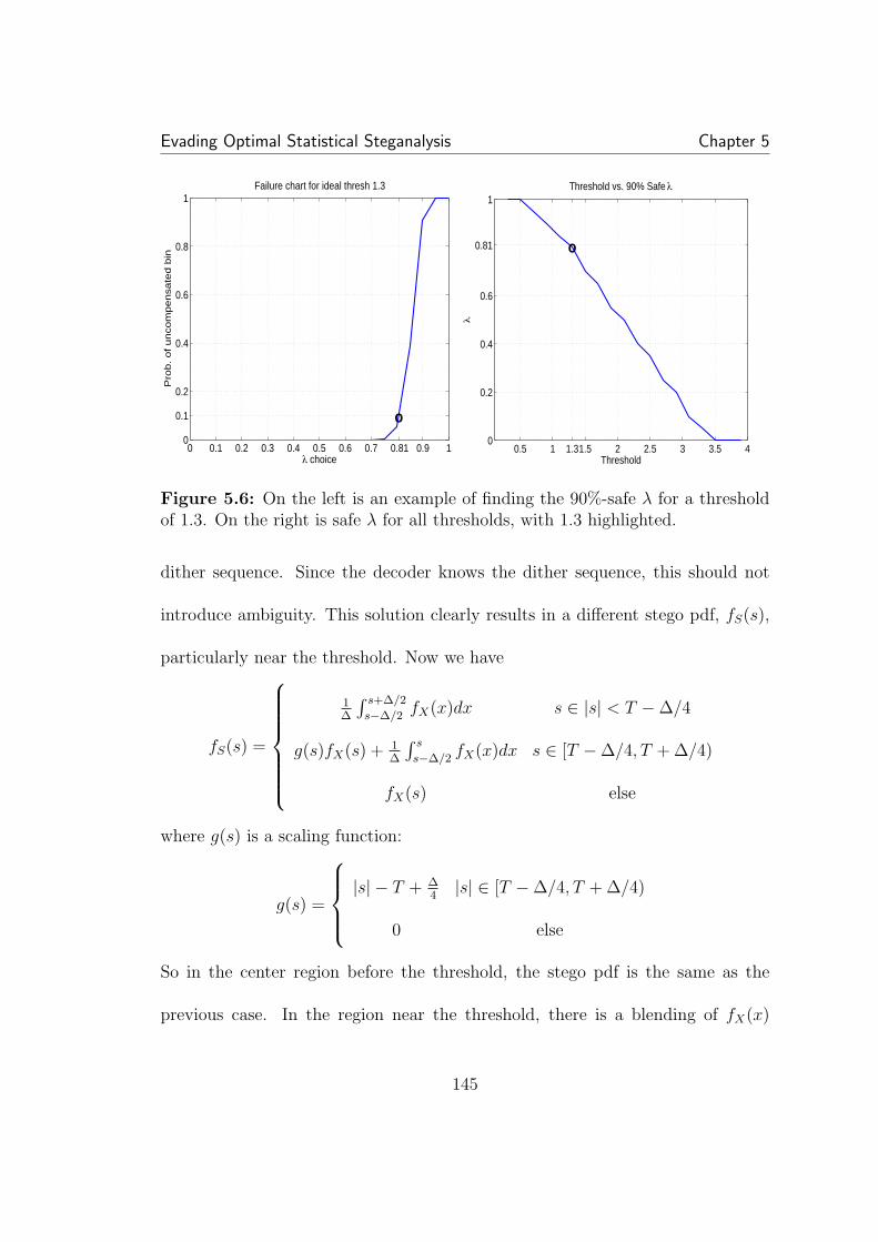
Evading Optimal Statistical Steganalysis Chapter 5
0 0.1 0.2 0.3 0.4 0.5 0.6 0.7 0.81 0.9 10
0.1
0.2
0.4
0.6
0.8
1Failure chart for ideal thresh 1.3
λ choice
Pro
b. of uncom
pensate
d b
in
o
0.5 1 1.31.5 2 2.5 3 3.5 40
0.2
0.4
0.6
0.81
1Threshold vs. 90% Safe λ
Thresholdλ
o
Figure 5.6: On the left is an example of finding the 90%-safe λ for a thresholdof 1.3. On the right is safe λ for all thresholds, with 1.3 highlighted.
dither sequence. Since the decoder knows the dither sequence, this should not
introduce ambiguity. This solution clearly results in a different stego pdf, fS(s),
particularly near the threshold. Now we have
fS(s) =
1∆
∫ s+∆/2
s−∆/2fX(x)dx s ∈ |s| < T −∆/4
g(s)fX(s) + 1∆
∫ s
s−∆/2fX(x)dx s ∈ [T −∆/4, T + ∆/4)
fX(s) else
where g(s) is a scaling function:
g(s) =
|s| − T + ∆
4|s| ∈ [T −∆/4, T + ∆/4)
0 else
So in the center region before the threshold, the stego pdf is the same as the
previous case. In the region near the threshold, there is a blending of fX(x)
145
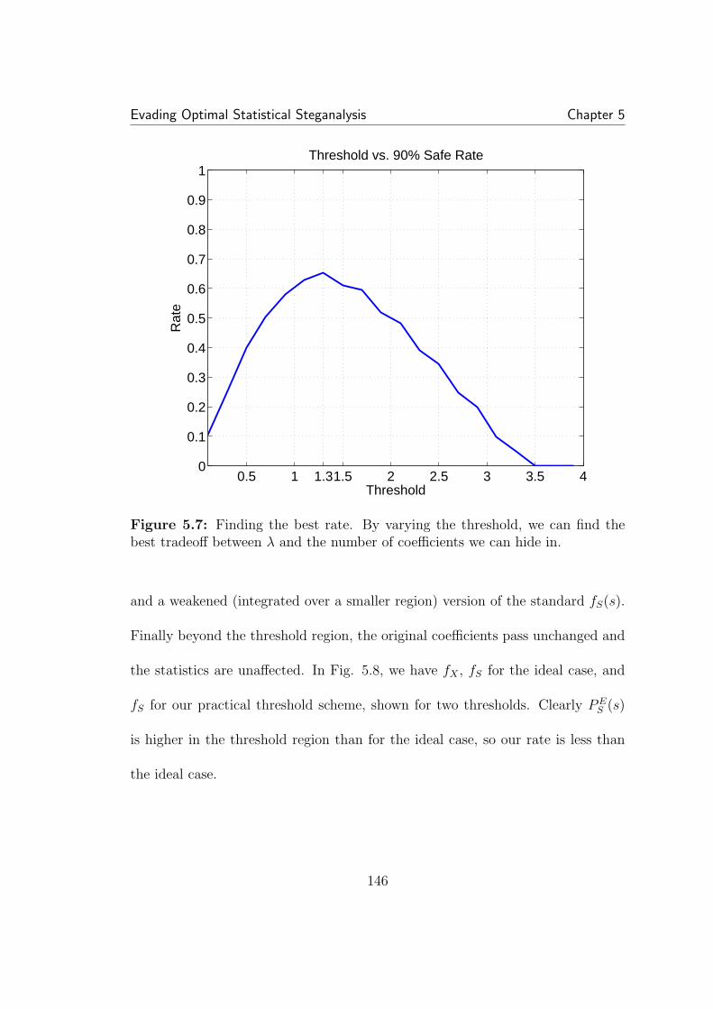
Evading Optimal Statistical Steganalysis Chapter 5
0.5 1 1.31.5 2 2.5 3 3.5 40
0.1
0.2
0.3
0.4
0.5
0.6
0.7
0.8
0.9
1Threshold vs. 90% Safe Rate
Threshold
Rat
e
Figure 5.7: Finding the best rate. By varying the threshold, we can find thebest tradeoff between λ and the number of coefficients we can hide in.
and a weakened (integrated over a smaller region) version of the standard fS(s).
Finally beyond the threshold region, the original coefficients pass unchanged and
the statistics are unaffected. In Fig. 5.8, we have fX , fS for the ideal case, and
fS for our practical threshold scheme, shown for two thresholds. Clearly PES (s)
is higher in the threshold region than for the ideal case, so our rate is less than
the ideal case.
146
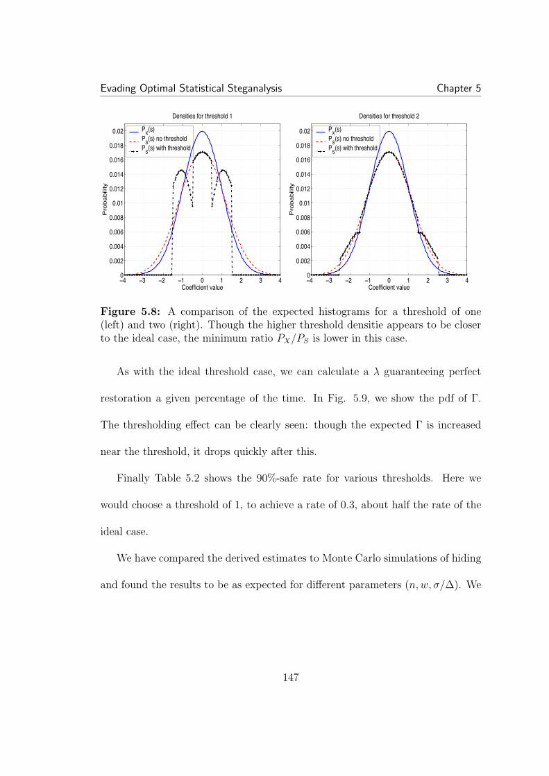
Evading Optimal Statistical Steganalysis Chapter 5
−4 −3 −2 −1 0 1 2 3 40
0.002
0.004
0.006
0.008
0.01
0.012
0.014
0.016
0.018
0.02
Densities for threshold 1
Coefficient value
Pro
babili
ty
PX(s)
PS(s) no threshold
PS(s) with threshold
−4 −3 −2 −1 0 1 2 3 40
0.002
0.004
0.006
0.008
0.01
0.012
0.014
0.016
0.018
0.02
Densities for threshold 2
Coefficient valueP
robabili
ty
PX(s)
PS(s) no threshold
PS(s) with threshold
Figure 5.8: A comparison of the expected histograms for a threshold of one(left) and two (right). Though the higher threshold densitie appears to be closerto the ideal case, the minimum ratio PX/PS is lower in this case.
As with the ideal threshold case, we can calculate a λ guaranteeing perfect
restoration a given percentage of the time. In Fig. 5.9, we show the pdf of Γ.
The thresholding effect can be clearly seen: though the expected Γ is increased
near the threshold, it drops quickly after this.
Finally Table 5.2 shows the 90%-safe rate for various thresholds. Here we
would choose a threshold of 1, to achieve a rate of 0.3, about half the rate of the
ideal case.
We have compared the derived estimates to Monte Carlo simulations of hiding
and found the results to be as expected for different parameters (n, w, σ/∆). We
147
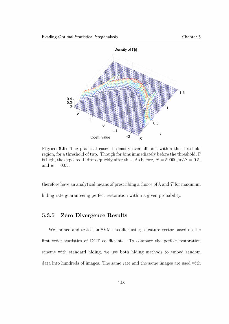
Evading Optimal Statistical Steganalysis Chapter 5
0
0.5
1
1.5
−2
−1
0
1
2
00.20.4
γ
Density of Γ[i]
Coeff. value
Figure 5.9: The practical case: Γ density over all bins within the thresholdregion, for a threshold of two. Though for bins immediately before the threshold, Γis high, the expected Γ drops quickly after this. As before, N = 50000, σ/∆ = 0.5,and w = 0.05.
therefore have an analytical means of prescribing a choice of λ and T for maximum
hiding rate guaranteeing perfect restoration within a given probability.
5.3.5 Zero Divergence Results
We trained and tested an SVM classifier using a feature vector based on the
first order statistics of DCT coefficients. To compare the perfect restoration
scheme with standard hiding, we use both hiding methods to embed random
data into hundreds of images. The same rate and the same images are used with
148
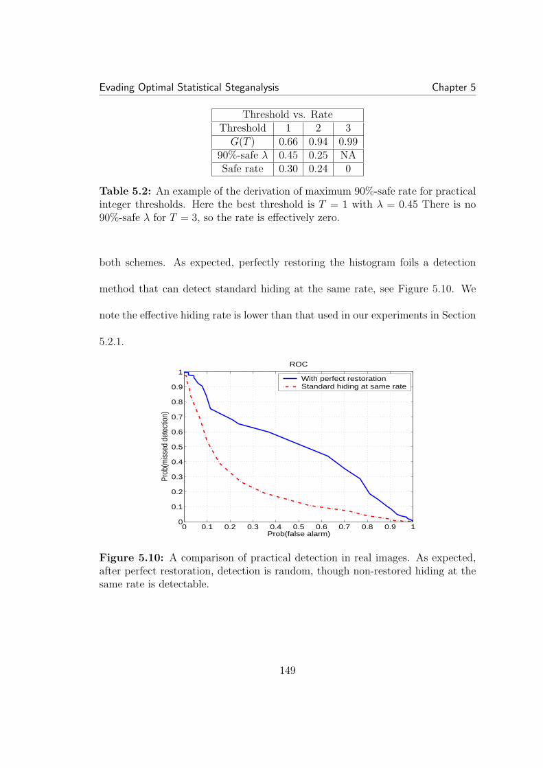
Evading Optimal Statistical Steganalysis Chapter 5
Threshold vs. RateThreshold 1 2 3
G(T ) 0.66 0.94 0.9990%-safe λ 0.45 0.25 NASafe rate 0.30 0.24 0
Table 5.2: An example of the derivation of maximum 90%-safe rate for practicalinteger thresholds. Here the best threshold is T = 1 with λ = 0.45 There is no90%-safe λ for T = 3, so the rate is effectively zero.
both schemes. As expected, perfectly restoring the histogram foils a detection
method that can detect standard hiding at the same rate, see Figure 5.10. We
note the effective hiding rate is lower than that used in our experiments in Section
5.2.1.
0 0.1 0.2 0.3 0.4 0.5 0.6 0.7 0.8 0.9 10
0.1
0.2
0.3
0.4
0.5
0.6
0.7
0.8
0.9
1ROC
Prob(false alarm)
Prob
(mis
sed
dete
ctio
n)
With perfect restorationStandard hiding at same rate
Figure 5.10: A comparison of practical detection in real images. As expected,after perfect restoration, detection is random, though non-restored hiding at thesame rate is detectable.
149

Evading Optimal Statistical Steganalysis Chapter 5
5.4 Hiding Rate for Zero Matrix Divergence
We now turn our attention to avoiding steganalysis that uses memory. As in
Chapter 4 we use a Markov chain model to include dependencies. To extend our
statistical compensation scheme discussed above, we now seek to compensate the
empirical matrix or joint histogram. In other words, we now consider changes to
pairs of values, rather than individual values.
5.4.1 Rate Distribution Derivation
In practice, it is difficult to implement a scheme to compensate pairs through-
out the entire image while still minimizing the mean square error introduced. On
the other hand, extending our analysis of histogram restoration is straightforward.
By doing so, we can estimate the best achievable hiding rate when considering
joint statistics in an idealized setting. Let fXn,Xn−1(xn, xn−1) be the joint pdf of
the cover, and fSn,Sn−1(sn, sn−1) the joint pdf of stego. As before, we assume the
steganalyst is using a histogram approximation. The expected joint histogram is
found similar to the one-dimension case (Eqn 5.1):
P(E)Xn,Xn−1
[i, j] =
∫ t[i]+w/2
t[i]−w/2
∫ t[j]+w/2
t[j]−w/2
fXn,Xn−1(xn, xn−1)dxndxn−1
Before proceeding, we note that each bin probability is lower than in the one-
dimensional case. For example, the probability of the pair (1.3, 1.4) is clearly be
150
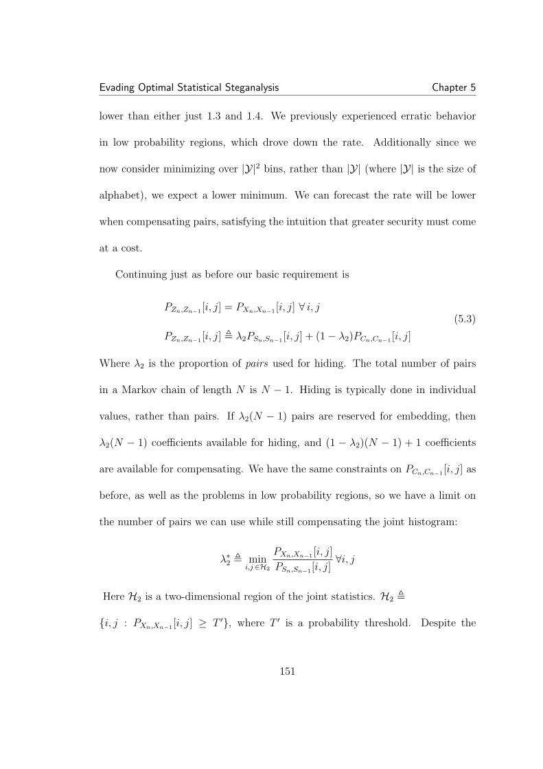
Evading Optimal Statistical Steganalysis Chapter 5
lower than either just 1.3 and 1.4. We previously experienced erratic behavior
in low probability regions, which drove down the rate. Additionally since we
now consider minimizing over |Y|2 bins, rather than |Y| (where |Y| is the size of
alphabet), we expect a lower minimum. We can forecast the rate will be lower
when compensating pairs, satisfying the intuition that greater security must come
at a cost.
Continuing just as before our basic requirement is
PZn,Zn−1 [i, j] = PXn,Xn−1 [i, j] ∀ i, j
PZn,Zn−1 [i, j] , λ2PSn,Sn−1 [i, j] + (1− λ2)PCn,Cn−1 [i, j]
(5.3)
Where λ2 is the proportion of pairs used for hiding. The total number of pairs
in a Markov chain of length N is N − 1. Hiding is typically done in individual
values, rather than pairs. If λ2(N − 1) pairs are reserved for embedding, then
λ2(N − 1) coefficients available for hiding, and (1 − λ2)(N − 1) + 1 coefficients
are available for compensating. We have the same constraints on PCn,Cn−1 [i, j] as
before, as well as the problems in low probability regions, so we have a limit on
the number of pairs we can use while still compensating the joint histogram:
λ∗2 , mini,j ∈H2
PXn,Xn−1 [i, j]
PSn,Sn−1 [i, j]∀i, j
Here H2 is a two-dimensional region of the joint statistics. H2 ,
{i, j : PXn,Xn−1 [i, j] ≥ T ′}, where T ′ is a probability threshold. Despite the
151
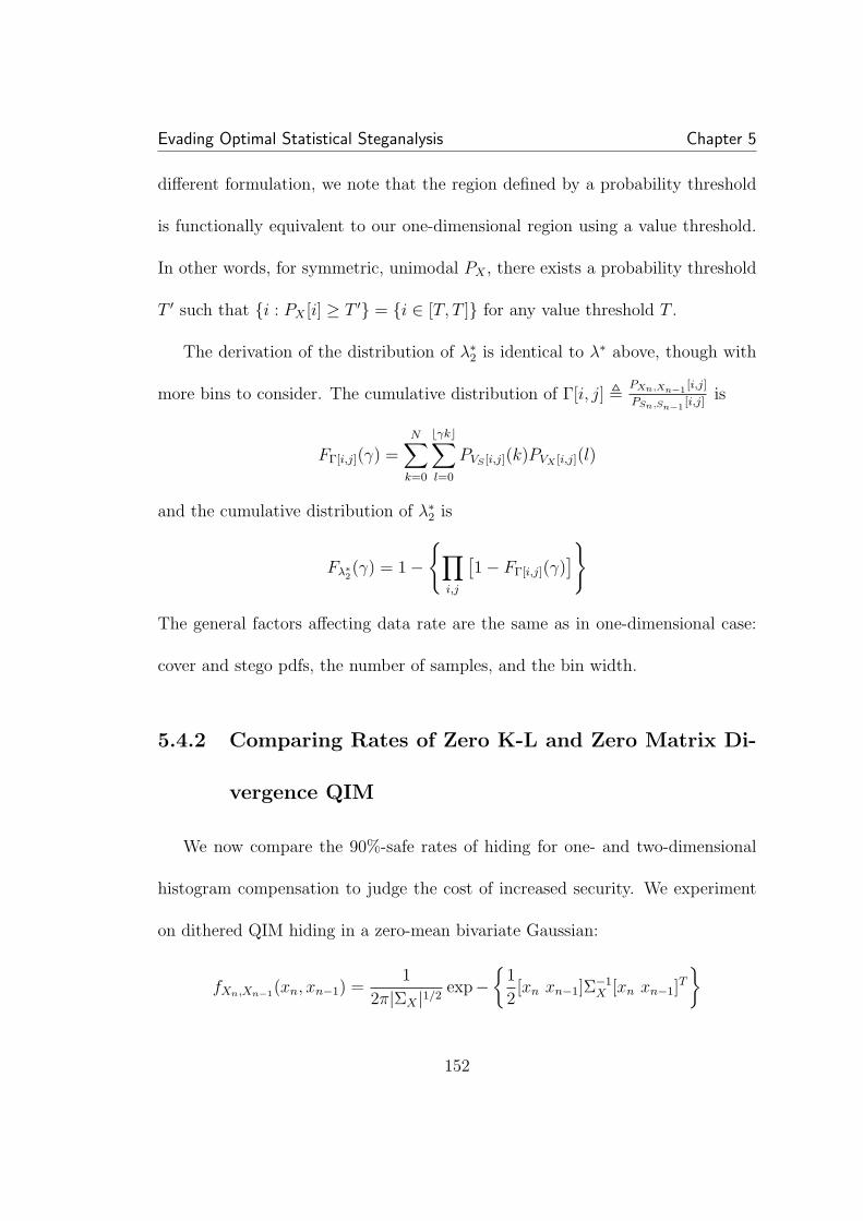
Evading Optimal Statistical Steganalysis Chapter 5
different formulation, we note that the region defined by a probability threshold
is functionally equivalent to our one-dimensional region using a value threshold.
In other words, for symmetric, unimodal PX , there exists a probability threshold
T ′ such that {i : PX [i] ≥ T ′} = {i ∈ [T, T ]} for any value threshold T .
The derivation of the distribution of λ∗2 is identical to λ∗ above, though with
more bins to consider. The cumulative distribution of Γ[i, j] ,PXn,Xn−1
[i,j]
PSn,Sn−1[i,j]
is
FΓ[i,j](γ) =N∑
k=0
bγkc∑l=0
PVS [i,j](k)PVX [i,j](l)
and the cumulative distribution of λ∗2 is
Fλ∗2(γ) = 1−
{∏i,j
[1− FΓ[i,j](γ)
]}
The general factors affecting data rate are the same as in one-dimensional case:
cover and stego pdfs, the number of samples, and the bin width.
5.4.2 Comparing Rates of Zero K-L and Zero Matrix Di-
vergence QIM
We now compare the 90%-safe rates of hiding for one- and two-dimensional
histogram compensation to judge the cost of increased security. We experiment
on dithered QIM hiding in a zero-mean bivariate Gaussian:
fXn,Xn−1(xn, xn−1) =1
2π|ΣX |1/2exp−
{1
2[xn xn−1]Σ
−1X [xn xn−1]
T
}
152
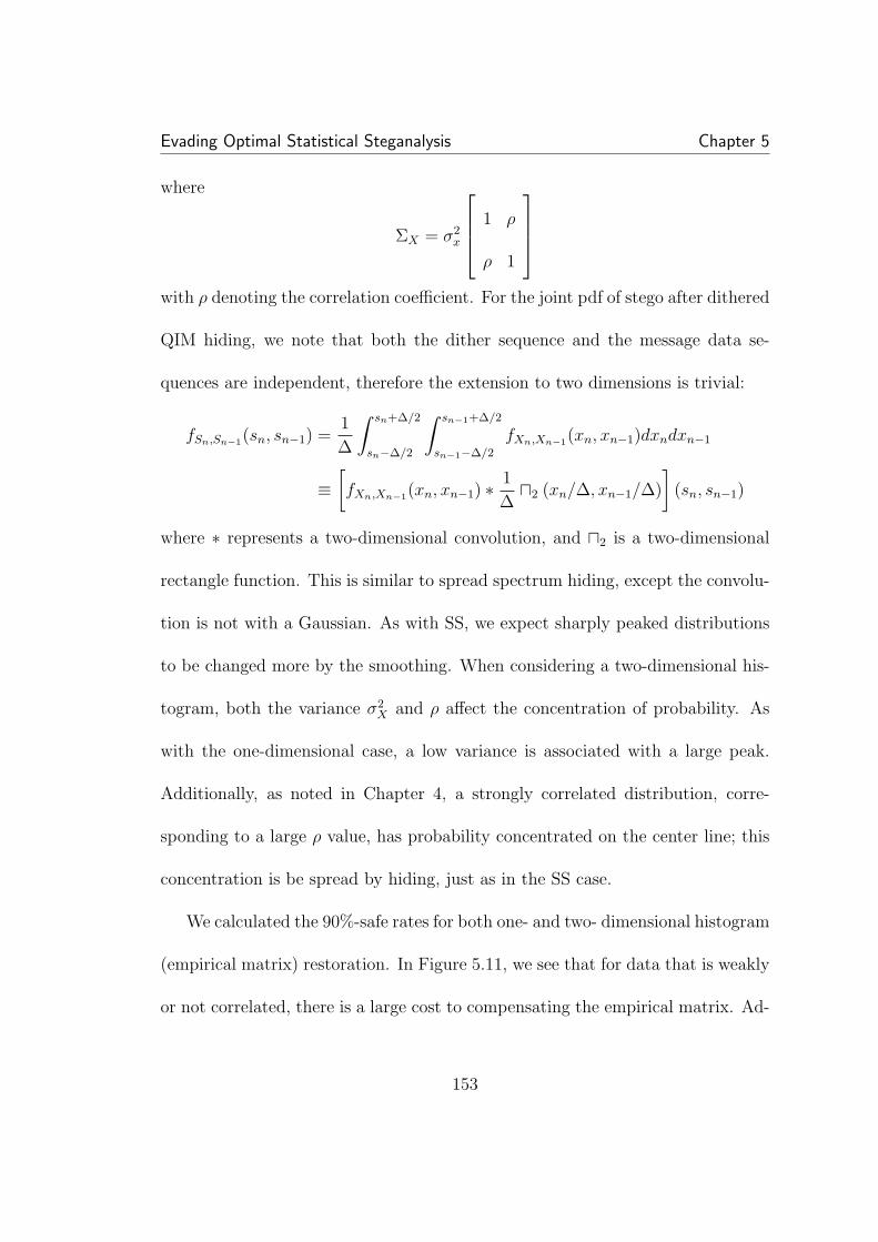
Evading Optimal Statistical Steganalysis Chapter 5
where
ΣX = σ2x
1 ρ
ρ 1
with ρ denoting the correlation coefficient. For the joint pdf of stego after dithered
QIM hiding, we note that both the dither sequence and the message data se-
quences are independent, therefore the extension to two dimensions is trivial:
fSn,Sn−1(sn, sn−1) =1
∆
∫ sn+∆/2
sn−∆/2
∫ sn−1+∆/2
sn−1−∆/2
fXn,Xn−1(xn, xn−1)dxndxn−1
≡[fXn,Xn−1(xn, xn−1) ∗
1
∆u2 (xn/∆, xn−1/∆)
](sn, sn−1)
where ∗ represents a two-dimensional convolution, and u2 is a two-dimensional
rectangle function. This is similar to spread spectrum hiding, except the convolu-
tion is not with a Gaussian. As with SS, we expect sharply peaked distributions
to be changed more by the smoothing. When considering a two-dimensional his-
togram, both the variance σ2X and ρ affect the concentration of probability. As
with the one-dimensional case, a low variance is associated with a large peak.
Additionally, as noted in Chapter 4, a strongly correlated distribution, corre-
sponding to a large ρ value, has probability concentrated on the center line; this
concentration is be spread by hiding, just as in the SS case.
We calculated the 90%-safe rates for both one- and two- dimensional histogram
(empirical matrix) restoration. In Figure 5.11, we see that for data that is weakly
or not correlated, there is a large cost to compensating the empirical matrix. Ad-
153

Evading Optimal Statistical Steganalysis Chapter 5
ditionally the security gain in this cases is quite small, as the divergence of the
histogram is nearly equal to the divergence of the empirical matrix. For trans-
form coefficients, which are only weakly correlated, it is probably not worthwhile
to consider joint statistics. However we are surprised to find that for strongly
correlated covers, the matrix compensation rate approaches and even passes the
histogram compensation rate. We note that since
PZ [i] =∑
j
PZn,Zn−1 [i, j]
then if PZn,Zn−1 = PXn,Xn−1 , then PZ = PX . Therefore a perfect matrix restoration
implies perfect histogram restoration, and a higher rate can be achieved for greater
security! Though this seems to violate intuition, we point out that the ratio
of distributions is non-linear, and it is difficult to guess results beforehand. In
particular, although these ratios are equivalent∑j PXn,Xn−1 [i, j]∑j PSn,Sn−1 [i, j]
=PX [i]
PS[i]
these are not ∑j
(PXn,Xn−1 [i, j]
PSn,Sn−1 [i, j]
)6= PX [i]
PS[i].
and we do not expect any obvious relationship between the distribution of Γ[i]
and Γ[i, j] .
There is a key caveat to this finding however. For the matrix restoration,
we have used a probability threshold to decide which bins to hide in. Though
154
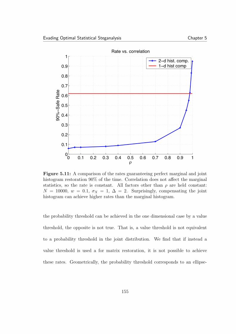
Evading Optimal Statistical Steganalysis Chapter 5
0 0.1 0.2 0.3 0.4 0.5 0.6 0.7 0.8 0.9 10
0.1
0.2
0.3
0.4
0.5
0.6
0.7
0.8
0.9
1
ρ
90%−
Saf
e R
ate
Rate vs. correlation
2−d hist. comp.1−d hist comp
Figure 5.11: A comparison of the rates guaranteeing perfect marginal and jointhistogram restoration 90% of the time. Correlation does not affect the marginalstatistics, so the rate is constant. All factors other than ρ are held constant:N = 10000, w = 0.1, σX = 1, ∆ = 2. Surprisingly, compensating the jointhistogram can achieve higher rates than the marginal histogram.
the probability threshold can be achieved in the one dimensional case by a value
threshold, the opposite is not true. That is, a value threshold is not equivalent
to a probability threshold in the joint distribution. We find that if instead a
value threshold is used a for matrix restoration, it is not possible to achieve
these rates. Geometrically, the probability threshold corresponds to an ellipse-
155
Evading Optimal Statistical Steganalysis Chapter 5
like region in the joint distribution, whereas the value threshold is a square region.
The former is better fitted to the distribution of correlated data. In particular,
the balance between the number of embedding coefficients and λ∗ is more difficult
to do with a square region. The smallest possible change in the threshold causes
a large change in both G(T ) and λ∗. Therefore using a square region (i.e. a value
threshold) reduces the rate significantly. In the one-dimensional case we had
practical difficulties implementing the value threshold, and our solution achieved
a lower rate than the ideal rate. We expect further difficulties with a probability
threshold, and in practice these rates are may be difficult to achieve.
5.5 Summary
We have analyzed a hiding scheme designed to increase security by explicit
restoration of the pdf. We believe there are two advantages of this approach over
earlier compensation schemes. First, continuous valued covers, for example, un-
compressed transform coefficients, can be used. Second, because a proven QIM
method is used for hiding, the scheme is robust against some noise, attacks, and
image processing. By first considering allowing a small amount of divergence be-
tween cover and stego by not compensating a small low-probability region, we find
the tradeoff using compensation is better than the tradeoff achieved by simply
156

Evading Optimal Statistical Steganalysis Chapter 5
embedding less. We continue the analysis be examining perfect compensation.
We derive expressions to evaluate the rate guaranteeing perfect security within a
specified probability for both the ideal case and a practical implementation. We
expand these results to the case of protecting against steganalysis using a level
of dependency. By comparing these results with the simpler case we find that,
theoretically, empirical matrix compensation can outperform histogram compen-
sation. However, this only occurs in very strongly correlated data, and caution
that it may be very difficult to achieve these results in practice.
157
Chapter 6
Future Work and Conclusions
The proliferation of steganographic tools has created a demand for powerful
means to detect hidden data. The primary focus of this dissertation is to employ
a systematic approach to the study of steganalysis allowing both the derivation of
optimal bounds and the design of practical solutions. Using a detection-theoretic
approach, we investigated the inherent detectability of several commonly used
data hiding techniques, devised methods to detect these schemes, and used this
knowledge to devise and analyze a means of escaping detection.
Though our approach has gained satisfying results in the study of steganog-
raphy, we acknowledge there are problems yet to be solved. We conclude with
a look to future research directions which we believe will advance the study of
stealthy transmission of, and interception of, hidden data in images.
158
Future Work and Conclusions Chapter 6
6.1 Improving Model of Images
We have seen that using a Markov chain image model has increased the ac-
curacy of our steganalysis results, by allowing one level of dependency. Markov
random field (MRF) models, with larger neighborhoods of dependency, have had
some success in characterizing images. Many other models [83, 80] for describ-
ing spatial and transform domain statistical characteristics have been proposed.
However, while a more complex model may be a more accurate representation
of image data, a problem with increasing the complexity of the model is the
increasing inaccuracy of estimates of the model for a given number of samples
[15].
Typically statistical models assume the distribution is the same for all image
pixels, that is, the random process is stationary. However we have seen some
data hiding methods [81, 37, 31] that adaptively embed data according to the
local statistics, suggesting that a careful steganalyst should consider a variation
in statistics across the image. A piece-wise stationarity assumption, in which
a different stationary random process is assumed for several regions within the
image, is perhaps a better way to model real images while remaining analyti-
cally tractable. There is however a significant challenge with this approach: how
to choose regions that accurately group statistically related pixels. Certainly a
159

Future Work and Conclusions Chapter 6
smaller region is more likely to follow a stationarity assumption, however a smaller
region has fewer samples with which to estimate the distribution of the region.
Grouping pixels from the same distribution is essentially image segmentation, a
very difficult problem and an active field of research. By leveraging the results of
this field, an appropriate means of selection may be found.
In addition to variation within an image, we have observed in our testing a
noticeable disparity in detector effectiveness according to the source of the cover
image. By source we mean both the scene represented in the image and the
technology used to create a digital representation of the scene. For example,
small sections of a very high resolution image are much more homogenous than a
lower resolution image of the same size. Assumptions based on stationarity and
strong correlation therefore work better for the former than the latter. We have
attempted to account for this in our experiments by using images from several
different sources; however the choice of an “ideal” natural image database remains
an ill-posed problem. To improve detection on images with widely varying sources,
for example images grabbed randomly off of the Internet, it may be beneficial to
use a two-stage classifier. The first stage classifies the image into rough groups
based on source, the second stage discriminates between cover and stego within
these groups.
160
Future Work and Conclusions Chapter 6
6.2 Accurate Characterization of Non-Optimal
Detection
A key advantage of the detection-theoretic approach is provable bounds on
detector performance giving a steganographer a guarantee of security. A decrease
in hiding rate is generally accepted to effect an increase in security. However, an-
ticipating optimal detection may be too pessimistic, causing a greater sacrifice of
rate than is actually necessary to avoid detection. Practical detectors will always
fall short of optimal, due to the insufficiency of information practically available.
In particular, the steganalyst’s lack of knowledge of the cover distribution means
she or he has to use general observations on natural images, either directly or
through supervised learning. If the exact cost to detector performance caused by
estimating this information could be accurately characterized, the steganographer
could hide at an increased rate while still remaining effectively stealthy. Addi-
tionally, the steganalyst will know when the practical limits of detection have
been reached. Accurately characterizing the difference between optimal detection
and the best that can be realistically done is a very challenging problem, but the
potential benefits are great.
161
Future Work and Conclusions Chapter 6
6.3 Summary
In this thesis we implemented a detection-theoretic approach to the analysis of
steganographic security from both the detector’s and hider’s point of view. This
theory is well-developed and is naturally suited to the steganalysis problem. This
approach allows us to estimate the performance of optimal statistical detection
of hiding in images.
In addition to characterizing optimal steganalysis under idealized conditions,
we developed methods for practical detection in realistic scenarios. Specifically,
we develop tools to detect three general classes of data hiding in natural images:
least significant bit (LSB), quantization index modulation (QIM), and spread
spectrum (SS).
Though powerful detection schemes exploiting image dependencies exist, sys-
tematic approaches to steganalysis have typically focused on an independent and
identically distributed (i.i.d.) assumption. We extend the detection-theoretic ap-
proach to the next logical step by using a Markov chain model of hiding media,
thus allowing a systematic approach using a measure of dependency.
Finally, we leveraged our steganalysis knowledge to design a system to evade
optimal steganalysis. In addition to designing a system which successfully reduces
the effectiveness of previously successful detection for dithered QIM, this analysis
162
Future Work and Conclusions Chapter 6
is also used to derive a formulation of the rate of secure hiding for arbitrary cover
distributions.
Steganalysis and steganography are complex problems, and there are many
avenues available for further exploration. Image data is difficult to succinctly
characterize. We note that a more complex image model could be used, allowing
for more accurate statistical description of images. Additionally, the detection
theory provides estimates of the performance of optimal steganalysis. However
optimal steganalysis is practically impossible. If the deviation from optimality
could be accurately characterized, an estimate of inherent practical detectability
may be possible. Finally we have generally focused on grayscale still images.
However the methods we presented here can be applied to the study of data
hiding in color images, video, and audio.
163
Bibliography
[1] V. Anantharam. A large deviations approach to error exponents in sourcecoding and hypothesis testing. IEEE Trans. on Information Theory,36(4):938–943, 1990.
[2] T. Aura. Practical invisibility in digital communication. Lecture Notes inComputer Science: 1st Int’l Workshop on Information Hiding, 1174:265–278, 1996.
[3] I. Avcibas, N. Memon, and B. Sankur. Steganalysis using image qualitymetrics. In Proc. IST/SPIE’s 13th Annual Symposium on Electronic Imag-ing Science and Technology, San Jose, CA, 2001.
[4] I. Avcibas, N. Memon, and B. Sankur. Image steganalysis with binarysimilarity measures. In Proceedings of ICIP, 2002.
[5] I. Avcibas, N. Memon, and B. Sankur. Steganalysis using image qualitymetrics. IEEE Trans. on Image Processing, 12(2):221–229, 2003.
[6] R. Blahut. Principles and practice of information theory. Addison Wesley,1987.
[7] R. Bohme and A. Westfeld. Breaking Cauchy model-based JPEG steganog-raphy with first-order statistics. In Proc. 9th ESORICS, France, Sep 2004.
[8] R. Bohme and A. Westfeld. Exploiting preserved statistics for steganalysis.In Proc. 6th Int’l Workshop on Information Hiding, 2004.
[9] A. Brown. S-tools 4.0, http://www.snapfiles.com/get/stools.html.
[10] C. Cachin. An information theoretic model for steganography. LectureNotes in Computer Science: 2nd Int’l Workshop on Information Hiding,1525:306–318, 1998.
164
Bibliography
[11] M. U. Celik, G. Sharma, and A. Tekalp. Universal image steganalysis usingrate-distortion curves. In Proc. IST/SPIE’s 16th Annual Symposium onElectronic Imaging Science and Technology, San Jose, CA, Jan 2004.
[12] R. Chandramouli, M. Kharrazi, and N. Memon. Image steganography andsteganalysis: Concepts and practices. In Proceedings of Second Int’l Work-shop on Digital Watermarking, pages 35–49, 2003.
[13] R. Chandramouli and N. Memon. Analysis of LSB based image steganog-raphy techniques. In Proceedings of ICIP, pages 1019–1022, 2001.
[14] B. Chen and G. Wornell. Quantization index modulation: A class of prov-ably good methods for digital watermarking and information embedding.IEEE Trans. Info. Theory, 47(4):1423–1443, May 2001.
[15] V. Cherkassky and F. Mulier. Learning From Data: Concepts, Theory, andMethods. John Wiley & Sons, Inc., 1988.
[16] K. L. Chung. Markov Chains with stationary transition probabilities. Spring-Verlag, 1960.
[17] M. Costa. Writing on dirty paper. IEEE Trans. Info. Theory, IT-29(3):439–441, May 1983.
[18] T. M. Cover and J. A. Thomas. Elements of Information Theory. Wiley,1991.
[19] I. Cox, J. Kilian, T. Leighton, and T. Shamoon. Secure spread spectrum wa-termarking for multimedia. IEEE Trans. on Image Processing, 6(12):1673–1687, 1997.
[20] O. Dabeer, K. Sullivan, U. Madhow, S. Chandrasekaran, and B. Manjunath.Detection of hiding in the least significant bit. In Proceedings of Conferenceon Information Sciences and Systems (CISS), 2003.
[21] O. Dabeer, K. Sullivan, U. Madhow, S. Chandrasekaran, and B. Manjunath.Detection of hiding in the least significant bit. IEEE Trans. on SignalProcessing, Supplement on Secure Media I, 52(10):3046–3058, 2004.
[22] A. Dembo and O. Zeitouni. Large Deviations Techniques and Applications.Springer, New York, 2 edition, 1998.
165
Bibliography
[23] S. Draper, P. Ishwar, D. Molnar, V. Prabhakaran, K. Ramchandran,D. Schonberg, and D. Wagner. An analysis of empirical PMF based testsfor least significant bit image steganography. In Proc. 7th Int’l Workshopon Information Hiding, 2005.
[24] S. Dumitrescu, X. Wu, and Z. Wang. Detection of LSB steganography viasample pair analysis. IEEE Trans. on Signal Processing, 51(7):1995–2007,2003.
[25] J. Eggers, R. Bauml, R. Tzschoppe, and B. Girod. Scalar Costa schemefor information embedding. IEEE Trans. on Signal Processing, 51(4):1003–1019, 2003.
[26] J. J. Eggers, R. Bauml, and B. Girod. A communications approach to imagesteganography. In Proc. IST/SPIE’s 14th Annual Symposium on ElectronicImaging Science and Technology, San Jose, CA, 2002.
[27] FortKnox, software: http://www.clickok.co.uk/steg/index.html.
[28] H. Farid. Detecting stenographic messages in digital images. Technicalreport, Dartmouth College, Computer Science, 2001.
[29] E. Franz. Steganography preserving statistical properties. In 5th Inter-national Working Conference on Communication and Multimedia Security,2002.
[30] J. Fridrich. Feature-based steganalysis for JPEG images and its implicationsfor future design of steganographic schemes. In Proc. of Sixth InformationHiding Workshop, May 2004.
[31] J. Fridrich and M. Goljan. Digital image steganography using stochasticmodulation. In Proc. IST/SPIE’s 15th Annual Symposium on ElectronicImaging Science and Technology, San Jose, CA, Jan 2003.
[32] J. Fridrich and M. Goljan. On estimation of secret message length in LSBsteganography in spatial domain. In Proc. IST/SPIE’s 16th Annual Sym-posium on Electronic Imaging Science and Technology, San Jose, CA, 2004.
[33] J. Fridrich, M. Goljan, and R. Du. Reliable detection of LSB steganographyin color and grayscale images. In Proc. ACM Workshop on MultimediaSecurity, Ottawa, Canada, 2001.
166
Bibliography
[34] J. Fridrich, M. Goljan, and D. Hogea. Attacking the OutGuess. In Pro-ceedings of ACM Workshop on Multimedia and Security, Juan-Pins, France,Dec 2002.
[35] J. Fridrich, M. Goljan, and D. Hogea. Steganalysis of JPEG images: Break-ing the F5 algorithm. In Lecture notes in computer science: 5th Interna-tional Workshop on Information Hiding, volume 2578, pages 310–323, 2002.
[36] J. Fridrich, M. Goljan, and D. Hogea. New methodology for breakingsteganographic techniques for JPEGs. In Proc. IST/SPIE’s 15th AnnualSymposium on Electronic Imaging Science and Technology, San Jose, CA,Jan 2003.
[37] J. Fridrich, M. Goljan, P. Lisonek, and D. Soukal. Writing on wet paper. InProc. IST/SPIE’s 17th Annual Symposium on Electronic Imaging Scienceand Technology, San Jose, CA, 2005.
[38] J. Fridrich, M. Goljan, and D. Soukal. Perturbed quantization steganog-raphy with wet paper codes. In Proc. of ACM Multimedia and SecurityWorkshop, Sep 2004.
[39] S. I. Gel’Fand and M. S. Pinsker. Coding for channel with random pa-rameters. Problems of Control and Information Theory, 9(1):19–31, Jan.1979.
[40] A. Gersho and R. Gray. Vector quantization and signal compression. KluwerAcademic Publishers, 1992.
[41] R. C. Gonzalez and R. Woods. Digital image processing. Addison Wesley,1992.
[42] A. Goteti and P. Moulin. QIM watermarking games. In Proceedings ofICIP, Singapore, Oct 2004.
[43] P. Guillon, T. Furon, and P. Duhamel. Applied public-key steganography. InProc. IST/SPIE’s 14th Annual Symposium on Electronic Imaging Scienceand Technology, San Jose, CA, 2002.
[44] A. Habibi. Comparison of n-th order DPCM encoder with linear transforma-tions and block quantization techniques. IEEE Trans. on CommunicationTechnology, COM-19(6):948–956, Dec 1971.
167
Bibliography
[45] J. J. Harmsen and W. A. Pearlman. Steganalysis of additive noise mode-lable information hiding. In Proc. IST/SPIE’s 15th Annual Symposium onElectronic Imaging Science and Technology, San Jose, CA, 2003.
[46] M. T. Hogan, N. J. Hurley, G. C. M. Silvestre, F. Balado, and K. M.Whelan. ML detection of steganography. In Proc. IST/SPIE’s 17th AnnualSymposium on Electronic Imaging Science and Technology, San Jose, CA,2005.
[47] InThePicture, software: http://www.intar.com/ITP/itpinfo.htm/.
[48] Invisible Secrets, software: http://www.invisiblesecrets.com/.
[49] JSTEG, software: http://www.theargon.com/archives/steganography/.
[50] A. K. Jain. Fundamentals of Digital Image Processing. Prentice-Hall, 1989.
[51] T. Joachims. Making large-Scale SVM Learning Practical. In B. Scholkopf,C. Burges, and A. Smola, editors, Advances in Kernel Methods - SupportVector Learning. MIT Press, 1999.
[52] N. F. Johnson, Z. Duric, and S. Jajodia. Information Hiding: Steganogra-phy and Watermarking - Attacks and Countermeasures. Kluwer AcademicPublishers, 2001.
[53] M. Kharrazi, H. T. Sencar, and N. Memon. Benchmarking steganographicand steganalysis techniques. In Proc. IST/SPIE’s 17th Annual Symposiumon Electronic Imaging Science and Technology, San Jose, CA, 2005.
[54] K. Li and X.-P. Zhang. Reliable adaptive watermarking scheme integratedwith JPEG2000. In Proceedings of ISISPA, Rome, Italy, 2003.
[55] E. T. Lin and E. J. Delp. A review of data of hiding in digital images. InProceedings of the Image Processing, Image Quality, Image Capture SystemsConference (PICS ’99), pages 274–278, Savannah, Georgia, 1999.
[56] S. Lyu and H. Farid. Detecting hidden messages using higher-order statisticsand support vector machines. In Lecture notes in computer science: 5thInternational Workshop on Information Hiding, volume 2578, 2002.
[57] S. Lyu and H. Farid. Steganalysis using color wavelet statistics and one-classsupport vector machines. In Proc. IST/SPIE’s 16th Annual Symposium onElectronic Imaging Science and Technology, San Jose, CA, 2004.
168
Bibliography
[58] B. Macq, J. Dittmann, and E. J. Delp. Benchmarking of image watermark-ing algorithms for digital rights managment. Proc. of the IEEE, 92(6):971–983, 2004.
[59] A. Martin, G. Sapiro, and G. Seroussi. Is image steganography natural?HP labs tech report HPL-2004-39, 7 March 2004.
[60] L. Marvel, C. G. Boncelet Jr., and C. T. Retter. Spread spectrum imagesteganography. IEEE Trans. on Image Processing, 8(8):1075–1083, 1999.
[61] M. K. Mihcak and R. Venkatesan. Blind image watermarking via derivationand quantization of robust semi-global statistics. In Proceedings of ICASSP,May 2002.
[62] M. K. Mihcak, R. Venkatesan, and M. Kesal. Cryptanalysis of discrete-sequence spread spectrum watermarks. Lecture Notes in Computer Science:5th Int’l Workshop on Information Hiding, 2578:226–246, 2003.
[63] P. Moulin and Y. Wang. New results on steganographic capacity. In Pro-ceedings of Conference on Information Sciences and Systems (CISS), 2004.
[64] S. Natarajan. Large deviations, hypothesis testing, and source coding forfinite Markov chains. IEEE Trans. on Information Theory, 31(3):360–365,1985.
[65] A. Papoulis. Probability, Random Variables, and Stochastic Processes.McGraw-Hill, 1965.
[66] R. L. Pickholtz, D. L. Schilling, and L. B. Milstein. Theory of spread-spectrum communications – a tutorial. IEEE Trans. on Communications,30(5):855–884, 1982.
[67] V. Poor. An introduction to signal detection and estimation. Springer, NY,1994.
[68] N. Provos. Defending against statistical steganalysis. In 10th USENIXSecurity Symposium, Washington DC, 2001.
[69] N. Provos and P. Honeyman. Detecting steganographic content on theinternet. In ISOC NDSS’02, San Diego, CA, 2002.
[70] A. Rangarajan and R. Chellappa. Markov random field models in imageprocessing. In The handbook of brain theory and neural networks, pages564–567, 1995.
169

Bibliography
[71] C. R. Rao. Linear Statistical Inference and Its Applications. John Wileyand Sons, 1965.
[72] B. Roue, P. Bas, and J.-M. Chassery. Improving LSB steganalysis usingmarginal and joint probabilistic distributions. In Proc. of ACM Multimediaand Security Workshop, pages 75–80, Sept 2004.
[73] J. J. K. O. Ruanaidh and T. Pun. Rotation, scale and translation invariantdigital image watermarking. In Proceedings of ICIP, pages 536–539, SantaBarbara, CA, 1997.
[74] StegoArchive.com: http://www.stegoarchive.com.
[75] P. Sallee. Model-based steganography. In Proceedings of Second Int’l Work-shop on Digital Watermarking, pages 154–167, 2003.
[76] P. Sallee. Model-based methods for steganography and steganalysis. Inter-national Journal of Image and Graphics (IJIG), 5(1):167–190, 2005.
[77] D. W. Scott. On optimal and data-based histograms. Biometrika, 66(3):605–10, 1979.
[78] M. Sidorov. Hidden Markov models and steganalysis. In Proc. of ACMMultimedia and Security Workshop, pages 63–67, Sept 2004.
[79] M. Sidorov. A statistical steganalysis for digital images. In Proc. of theInternational I and S Workshop, pages 34–36, Jan 2004.
[80] E. Simoncelli. Statistical models for images: Compression restoration andsynthesis. In Proceedings of 31st Asilomar Conference on Signals, Systemsand Computers, Pacific Grove, CA, Nov. 1997.
[81] K. Solanki, N. Jacobsen, U. Madhow, B. S. Manjunath, and S. Chandra-sekaran. Robust image-adaptive data hiding based on erasure and errorcorrection. IEEE Transactions on Image Processing, 13(12):1627–1639, Dec2004.
[82] K. Solanki, K. Sullivan, U. Madhow, B. S. Manjunath, and S. Chandraseka-ran. Statistical restoration for robust and secure steganography. To appearICIP 2005.
[83] A. Srivastava, A. Lee, E. Simoncelli, and S.-C. Zhu. On advances in sta-tistical modeling of natural images. Journal of Mathematical Imaging andVision, 18:17–33, 2003.
170
Bibliography
[84] K. Sullivan, Z. Bi, U. Madhow, S. Chandrasekaran, and B. S. Manjunath.Steganalysis of quantization index modulation data hiding. In Proceedingsof ICIP, pages 1165–1168, Singapore, Oct 2004.
[85] K. Sullivan, O. Dabeer, U. Madhow, B. Manjunath, and S. Chandrasekaran.LLRT based detection of LSB hiding. In Proceedings of ICIP, volume 1,pages 497–500, Barcelona, Spain, Sep 2003.
[86] K. Sullivan, U. Madhow, S. Chandrasekaran, and B. S. Manjunath. Ste-ganalysis of spread spectrum data hiding exploiting cover memory. In Proc.IST/SPIE’s 17th Annual Symposium on Electronic Imaging Science andTechnology, San Jose, CA, Jan 2005.
[87] K. Sullivan, U. Madhow, B. S. Manjunath, and S. Chandrasekaran. Ste-ganalysis of Markov cover data with applications to images. Submitted toIEEE Trans. on Information Forensics and Security.
[88] R. Tzschoppe, R. Bauml, J. B. Huber, and A. Kaup. Steganographic sys-tem based on higher-order statistics. In Proc. IST/SPIE’s 15th AnnualSymposium on Electronic Imaging Science and Technology, San Jose, CA,Jan 2003.
[89] R. van Schyndel, A. Tirkel, and C. Osborne. A digital watermark. InProceedings of ICIP, volume 2, pages 86–90, Austin, TX, 1994.
[90] R. Venkatesan and M. H. Jakubowski. Image watermarking with betterresilience. In Proceedings of ICIP, Vancouver, British Columbia, Canada,2000.
[91] R. Venkatesan, V. Vazirani, and S. Sinha. A graph theoretic approachto software watermarking. Lecture Notes in Computer Science: 4th Int’lWorkshop on Information Hiding, 2137:157–168, 2001.
[92] M. Vetterli and C. Herley. Wavelets and filter banks: Theory and design.IEEE Transactions on Signal Processing, 40(9):2207–2232, 1992.
[93] R. F. Walker, P. Jackway, and I. Longstaff. Improving co-occurrence matrixfeature discrimination. In Proc. of Digital Image Computing: Techniquesand Applications (DICTA), pages 643–648, Dec 1995.
[94] G. K. Wallace. The JPEG still picture compression standard. Commun-ications of the ACM, 34(4):30–44, 1991.
171
Bibliography
[95] M. Wand. Data-based choice of histogram bin width. The American Statis-tician, 51(1):59–64, Feb 1997.
[96] M. Wand and M. Jones. Kernel Smoothing. Chapman & Hall, 1995.
[97] Y. Wang and P. Moulin. Steganalysis of block-DCT steganography. In Proc.IEEE Workshop on Statistical Signal Processing, St Louis, MO, Sep 2003.
[98] Y. Wang and P. Moulin. Steganalysis of block-structured stegotext. InProc. IST/SPIE’s 16th Annual Symposium on Electronic Imaging Scienceand Technology, San Jose, CA, 2004.
[99] A. Westfeld. High capacity despite better steganalysis (F5 - a stegano-graphic algorithm). In Lecture notes in computer science: 4th InternationalWorkshop on Information Hiding, volume 2137, pages 289–302, 2001.
[100] A. Westfeld and A. Pfitzmann. Attacks on steganographic systems. In Lec-ture notes in computer science: 3rd International Workshop on InformationHiding, 1999.
[101] R. Wolfgang and E. Delp. A watermark for digital images. In Proceedingsof ICIP, pages 219–222, Lausanne, Switzerland, 1996.
[102] R. B. Wolfgang, C. I. Podilchuk, and E. J. Delp. The effect of matchingwatermark and compression transforms in compressed color images. InProceedings of ICIP, Chicago, Illinois, Oct. 1998.
[103] J. J. Yu, J. W. Han, S. C. O, S. Lee, and I. H. Park. A secure steganographicscheme against statistical analyses. In Lecture Notes in Computer Science:Proceedings of Second Int’l Workshop on Digital Watermarking, volume2939, pages 497–507, 2004.
[104] R. Zamir, S. Shamai, and U. Erez. Nested linear/lattice codes for structuredmultiterminal binning. IEEE Trans. on Information Theory, 48(6):1250–1276, 2002.
[105] O. Zeitouni, J. Ziv, and N. Merhav. When is the generalized likelihood ratiotest optimal. IEEE Transactions on Information Theory, 38(5):1597–1602,1992.
[106] T. Zhang and X. Ping. A new approach to reliable detection of LSBsteganography in natural images. Signal Processing, 83(10):2085–2093,2003.
172
Bibliography
[107] J. Zolner, H. Federrath, H. Klimant, A. Pfitzmann, R. Piotraschke, A. West-feld, G. Wicke, and G. Wolf. Modeling the security of steganographic sys-tems. In Lecture notes in computer science: 2nd International Workshopon Information Hiding, volume 1525, pages 345–355, 1998.
173
Appendix A
Glossary of Symbols andAcronyms
List of Symbols
n, m, i, j, k various indexes, n is typically a sample index, i, j a value or bin index
A acceptance region of detector, page 38
A regularity constraint matrix, page 52
α probability of false alarm, or SS scaling parameter page 38 or 91
B hidden message bits, page 43
Bl blockiness measure, page 89
C output of standard quantizer or compensating coefficients, page 65 or 127
c denotes complement of a set, general use
C compensated region, page 129
D dither value for dithered QIM, or SS message bearing signal, page 67 or page90
D(·||·) Kullback-Leibler divergence (relative entropy), page 41
D(M(X),M(S)) matrix divergence between Markov chains X and S, page 85
δ(·) generic detector, page 38
174

Glossary of Symbols and Acronyms Chapter A
∆∗ step size for uniform scaler quantization, page 66
∆ step size for uniform scaler QIM, page 63
ηij number of transitions from i to j in Markov chain, page 83
ε bound on Kullback-Leibler divergence, page 30
fX(x), fS(s) probability density function (pdf) of cover and stego, page 126
FX(x) cumulative distribution function of random variable X: P (X ≤ x), generaluse
g(·) scaling function for practical threshold, page 145
G(·) number of embeddable coefficients as a function of threshold, page 143
Γ random variable, ratio of cover histogram to stego histogram, page 134
γ value of Γ, page 134
H(·) entropy of random variable, general use
Hb(·) entropy of binary random variable, page 27
H0, H1 cover, stego hypotheses, page 37
H hiding region for zero divergence statistical compensation, page 142
I number of bins, page 126
K composite hypothesis of stego hiding at any rate, page 45
κ ratio of matrix divergence to K-L divergence, page 86
L(·) log-likelihood statistic, page 39
L(·)χ2 chi-squared statistic, page 48
Lapprox.(·) approximate log-likelihood statistic, page 51
λ percentage of coefficients used for hiding, page 127
λ2 percentage of pairs used for hiding, joint compensation case, page 151
λ∗ percentage of coefficients available for hiding, perfect compensation, page 129
175
Glossary of Symbols and Acronyms Chapter A
λ∗2 same as λ∗ for joint compensation case, page 151
M empirical matrix of Markov chain, page 85
M(X),M(S) cover, stego empirical matrices, page 85
N number of samples, page 37
PX , PS function form of PMFs of cover, stego, page 65
P (E) probability of event E, general use
p(X),p(S) vector form of PMF cover and stego, page 40
p(X) estimate of cover PMF, page 51
qb quantizer indexed by message, page 62
q estimated PMF of received data (normalized histogram), page 40
QR matrix corresponding to linear transformation of LSB hiding at rate R, page44
Q(·) complementary Gaussian function, page 47
R hiding rate, page 43
R real line
u(t) rectangular function : u(t + 1/2)− u(t− 1/2), page 138
S, s stego random variable, value of stego random variable, page 37
T threshold for statistical compensation, page 142
T Markov chain transition matrix, page 83
σX standard deviation of random variable X
τ threshold for hypothesis test, page 38
w bin width of histogram, page 64
X, x cover random variable, value of cover random variable, page 37
X ∗ quantization range (Voronoi region) for uniform scalar quantization, page 65
176
Glossary of Symbols and Acronyms Chapter A
X quantization range (Voronoi region) for uniform scalar QIM, page 66
χ2 closeness-of-fit statistic, used for LSB detection, page 15
{Yn}Nn=1 received data samples, page 37
y received data vector, page 40
Y alphabet of data, page 38
Z statistically compensated stego, page 127
Zn indicator vector, page 46
List of Acronyms
AWGN additive white Gaussian noise
bpp bits per pixel
bpnz-DCT bits per non-zero DCT coefficient
CACD Canon digital camera
CPCD Corel photo CD
COM center of mass
DCT discrete cosine transform
DFT discrete Fourier transform
DWT discrete wavelet transform
DOQQ digital orthophoto quarter-quadrangle (Set of aerial images.)
HCF histogram characteristic function
MISE mean integrated squared error
HMM hidden Markov model
HPDM histogram-preserving data-mapping
HVS human visual system
IQM image quality metrics
177
Glossary of Symbols and Acronyms Chapter A
i.i.d. independent and identically distributed
JPEG joint photographic experts group (Image compression schemes.)
K-L Kullback-Leibler
KLT Karhunen-Loeve transform
LSB least significant bit
LRT likelihood ratio test
LLRT log likelihood ratio test
MC Markov chain
MCR message to cover (power) ratio
MRF Markov random field
MSE mean squared error
MMSE minimum mean squared error
pdf probability density function
PNG portable network graphics (Image compression scheme.)
PMF probability mass function
PR psuedorandom
PSNR peak signal to noise ratio
QIM quantization index modulation
ROC receiver operating characteristics
RS regular/singular (Used to denote detection method using sets with thesenames.)
SS spread spectrum
SSIS spread spectrum image steganography
SVM support vector machine
178


![Enhancing Image Steganalysis with Adversarially Generated ... · a popular steganalysis tool which implements several di erent steganalysis al-gorithms including Primary Sets [4],](https://static.cupdf.com/doc/110x72/600f6c5dec5d6219b63bacd9/enhancing-image-steganalysis-with-adversarially-generated-a-popular-steganalysis.jpg)