Fitting of Stochastic Telecommunication Network Models

via Distance Measures and Monte–Carlo Tests

C. Gloaguen 1 F. Fleischer 2 H. Schmidt 3 V. Schmidt 3

14th November 2005

Abstract

We explore real telecommunication data describing the spatial geometrical structure of

an urban region and we propose a model fitting procedure, where a given choice of dif-

ferent non–iterated and iterated tessellation models is considered and fitted to real data.

This model fitting procedure is based on a comparison of distances between character-

istics of sample data sets and characteristics of different tessellation models by utilizing

a chosen metric. Examples of such characteristics are the mean length of the edge–set

or the mean number of vertices per unit area. In particular, after a short review of a

stochastic–geometric telecommunication model and a detailed description of the model

fitting algorithm, we verify the algorithm by using simulated test data and subsequently

apply the procedure to infrastructure data of Paris.

Keywords : Telecommunication network modelling, stochastic geometry,

access network, random tessellations, statistical fitting, Monte–Carlo

tests

1France Télécom R&D RESA/NET/NSO 92794 Issy Moulineaux Cedex 9, France2Department of Applied Information Processing and Department of Stochastics, University of Ulm, 89069

Ulm, Germany3Department of Stochastics, University of Ulm, 89069 Ulm, Germany

1

2

1 Introduction

Spatial stochastic models for telecommunication networks have been developed in recent years

as an alternative to more traditional economical approaches to cost measurement and strate-

gic planning. These models allow for incorporation of the stochastic and geometric features

observed in telecommunication networks. By taking the geometric structure of network ar-

chitectures into consideration, network models using tools of stochastic geometry offer a

more relevant view to location-dependent network characteristics than conventional network

models. The probabilistic setting reflects the network’s variability in time and space.

Popular examples of networks where stochastic–geometric models have been considered so far

are switching networks, multi-cast networks, and mobile telecommunication systems. These

new models based on stochastic geometry include Poisson–Voronoi aggregated tessellations

(Bacelli et al. (1996), Tchoumatchenko and Zuyev (2001)), superpositions of Poisson–Voronoi

tessellations (Baccelli, Gloaguen and Zuyev (2000)), spanning trees (Bacccelli, Kofman and

Rougier (1999), Baccelli and Zuyev (1996)), and coverage processes (Baccelli and Blaszczyszyn

(2001)).

In the following, we focus on telecommunication access networks that can be regarded as

the most important part of telecommunication network modelling, since roughly 50% of the

total capital investment made in these networks is made in the access network. With such

large investments at stake, and possibly evoluting subscriber populations, it is important to

find appropriate models for cost evaluation, performance analysis, and strategic planning of

access networks.

The access network or local loop is the part of the network connecting a subscriber to its cor-

responding Wire Center Stations (WCS). The hierarchical physical link is made via network

components: a Network Interface Device (ND), secondary and primary cabinets (CS and CP)

and a Service Area Station (SAI) as shown in Figure 1(a). A serving zone is associated to

each WCS; the subnetwork gathering all the links between the WCS and the subcribers lying

in its serving zone displays a tree structure (Figure 1(b)).

The most important feature about the access network is that it is the place where the telecom-

munication network fits in the town and country planning. For urban networks considered

here this means the urban architecture and street system.

Significant research in studying access networks has taken place in recent years with the so–

3

SAICPCSND

feeder cabledistribution cableservice wire

transportdistribution

WCSCPCP

connection

SAI

SAI

CP

WCS

CS

SAI

SAI

(a) Hierarchical physical link between a

subscriber and its Wire Center Station (WCS)

(b) Tree structure of a WCS subnetwork not

displaying the links between ND and CS

Figure 1: Hierachical structure of access networks

called Stochastic Subscriber Line Model (SSLM); see Gloaguen et.al. (2002) and Maier (2003).

The SSLM is a stochastic–geometric model and offers tools in order to describe the spatial

irregularity as well as the geometric features of access networks and allows for stochastic

econometrical analysis, like the analysis of connection costs. Particularly, it provides sim-

ple mean value formulae for network characteristics used for cost evaluation, performance

analysis, and strategic planning.

The modelling framework of the SSLM is subdivided into the Network Geometry Model, the

Network Component Model and the Network Topology Model. The Network Geometry Model

represents the cable trench system, which is located along the infrastructure system of a

city or of a country. Random iterated tessellations (see e.g., Maier and Schmidt (2003)) can

be used to describe this cable trench system. Subsequently the Network Component Model

localizes the technical network components on the geometry using Poisson processes on lines

or in the plane (Figure 2 (a)). To complete the picture, the Network Topology Model builds

up the link between a subscriber and the corresponding WCS following the shortest path

along the trench system (Figure 2 (b)).

Since the geometry of the infrastructure, i.e., the road system, is the basis of the access

network, an important task is the choice of an appropriate tessellation model given simulated

or real infrastructure data. In particular, three basic Poisson–type tessellation models are

considered, out of which iterated tessellation models can be constructed. These basic models

are called Poisson line tessellations (PLT), Poisson–Voronoi tessellations (PVT), and Poisson–

Delaunay tessellations (PDT).

In the present paper, an approach for a model choice is presented, which is based on the

4

(a) Realization of Network Geometry and

Network Component Models

(b) Shortest path analysis in the frame of the

Network Topology Model

Figure 2: Realization of the Stochastic Subscriber Line Model

minimization of distance measures between characteristics of input data and computed values

of these characteristics using theoretical formulae valid for random tessellation models. Input

data can be estimated characteristics both from real infrastructure data as well as from

realizations of random tessellations. The latter part is important in order to verify the

correctness of the model choice procedure.

In particular, in Section 2, a brief account of some basic notions of stochastic geometry is

given and the theoretical tessellation models we are going to use are presented.

In Section 3, the model choice procedure is described. To compare input data and theoretical

tessellation models, characteristics that describe the structural properties of the considered

data are used. Examples of such characteristics are the expected number of vertices or the

expected total length of the edges. Therefore, we need appropriate estimators for these

characteristics first. Notice that, subsequent to the identification of the optimal model, this

choice can be tested by using well–known Monte–Carlo test techniques (Stoyan and Stoyan

(1994)). The section closes with numerical examples, where input data is derived from

simulated realizations of random tessellations.

Finally, in Section 4, we consider real infrastructure data of Paris (see Figure 3). The data

consist of line segments. Each line segment has an attached mark describing the type of road

this segment belongs to. Hence for example, it is possible to distinguish between main roads

5

and side streets. A preprocessing of raw data is necessary in order to obtain a tessellation

that consists of polygonal cells. Subsequently, it is possible to measure characteristics similar

to those described above for simulated data.

Figure 3: Real infrastructure data of Paris

Notice that, after having chosen an optimal model for the road system, the next logical step

is to apply shortest paths algorithms to analyze connections between subscribers and their

corresponding WCS–station. A short outlook at the end of this paper gives insight how such

analysis can be performed, the results of which can be found in Gloaguen et al. (2005a,

2005b).

All programming work for the extensive simulation studies has been done using methods

from the GeoStoch library. This JAVA–based library comprises software tools designated to

analyze data with methods from stochastic geometry; see Mayer, Schmidt and Schweiggert

(2004) and http://www.geostoch.de.

2 Mathematical background

In this section, the basic mathematical notation used in the present paper is introduced and

a brief account of some relevant notions of stochastic geometry is given. Particularly, we put

emphasis on the introduction of random (iterated) tessellations, which are used as models for

the road system in the SSLM. For a detailed discussion of the mathematical background, it

is referred to the literature, for example Schneider and Weil (2000) and Stoyan, Kendall and

Mecke (1995). Further information about random (iterated) tessellations can also be found,

e.g. in Maier and Schmidt (2003), Møller (1989), and Okabe et al. (2000).

6

2.1 Basic notations

The abbreviations int B, ∂B, and Bc are used to denote the interior, the boundary, and the

complement of a set B ⊂ IR2, respectively, where IR2 denotes the 2–dimensional Euclidean

space. Notice that by |B| we denote the 2–dimensional Lebesgue measure for an arbitrary

measurable set B ∈ IR2, i.e. |B| is the area of B.

The families of all closed sets, compact sets, and convex bodies (compact and convex sets) in

IR2 are denoted by F , K, and C, respectively. Recall that a random closed set Ξ in IR2 is a

measurable mapping Ξ : Ω → F from some probability space (Ω,A, IP) into the measurable

space (F ,B(F)), where B(F) denotes the smallest σ–algebra of subsets of F that contains

all sets F ∈ F , F ∩ K = ∅ for any K ∈ K. Particularly, the random closed set Ξ is

called a random compact set or a random convex body if IP(Ξ ∈ K) = 1 or IP(Ξ ∈ C) = 1,

respectively.

2.2 Random tessellations

A tessellation in IR2 is a countable family τ = Cnn≥1 of convex bodies Cn ∈ C such

that int Cn = ∅ for all n, int Cn ∩ int Cm = ∅ for all n = m,⋃

n≥1 Cn = IR2, and∑n≥1 1ICn∩K =∅ < ∞ for any K ∈ K. Notice that the sets Cn, called the cells of τ , are

polygons in IR2. The family of all tessellations in IRd is denoted by T . A random tessellation

Ξnn≥1 in IRd is a sequence of random convex bodies Ξn such that IP(Ξnn≥1 ∈ T ) = 1.

Notice that a random tessellation Ξnn≥1 can also be considered as a marked point process∑n≥1 δ[α(Ξn),Ξ0

n], where α : C′ → IRd, C′ = C \ ∅, is a measurable mapping such that

α(C) ∈ C and α(C +x) = α(C)+x for any C ∈ C′ and x ∈ IRd, and where Ξ0n = Ξn −α(Ξn)

is the centered cell corresponding to Ξn which contains the origin. The point α(C) ∈ IRd is

called the associated point of C and can be chosen, for example, to be the lexicographically

smallest point of C.

2.3 Examples of non–iterated random tessellations

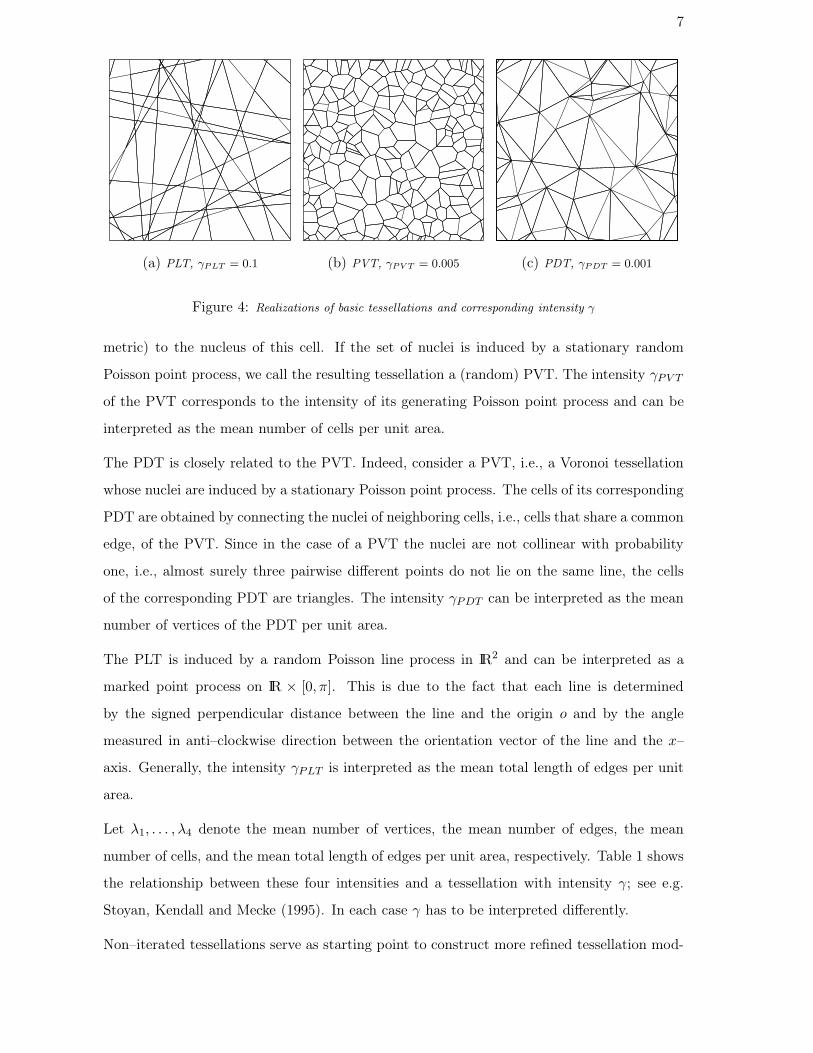
Figure 4 shows realizations of our three basic non–iterated tessellation models, namely the

PLT, the PVT, and the PDT.

The cells of a (deterministic) Voronoi tessellation are convex polygons in IR2, namely the

closure of all planar points which are closest (in the sense of the 2-dimensional Euclidean

7

(a) PLT, γPLT = 0.1 (b) PVT, γPV T = 0.005 (c) PDT, γPDT = 0.001

Figure 4: Realizations of basic tessellations and corresponding intensity γ

metric) to the nucleus of this cell. If the set of nuclei is induced by a stationary random

Poisson point process, we call the resulting tessellation a (random) PVT. The intensity γPV T

of the PVT corresponds to the intensity of its generating Poisson point process and can be

interpreted as the mean number of cells per unit area.

The PDT is closely related to the PVT. Indeed, consider a PVT, i.e., a Voronoi tessellation

whose nuclei are induced by a stationary Poisson point process. The cells of its corresponding

PDT are obtained by connecting the nuclei of neighboring cells, i.e., cells that share a common

edge, of the PVT. Since in the case of a PVT the nuclei are not collinear with probability

one, i.e., almost surely three pairwise different points do not lie on the same line, the cells

of the corresponding PDT are triangles. The intensity γPDT can be interpreted as the mean

number of vertices of the PDT per unit area.

The PLT is induced by a random Poisson line process in IR2 and can be interpreted as a

marked point process on IR × [0, π]. This is due to the fact that each line is determined

by the signed perpendicular distance between the line and the origin o and by the angle

measured in anti–clockwise direction between the orientation vector of the line and the x–

axis. Generally, the intensity γPLT is interpreted as the mean total length of edges per unit

area.

Let λ1, . . . , λ4 denote the mean number of vertices, the mean number of edges, the mean

number of cells, and the mean total length of edges per unit area, respectively. Table 1 shows

the relationship between these four intensities and a tessellation with intensity γ; see e.g.

Stoyan, Kendall and Mecke (1995). In each case γ has to be interpreted differently.

Non–iterated tessellations serve as starting point to construct more refined tessellation mod-

8

Table 1: Values of λ1, . . . , λ4 for a given tessellation with intensity γ

Tessellation λ1 λ2 λ3 λ4

PLT 1πγ2 2

πγ2 1πγ2 γ

PVT 2γ 3γ γ 2√

γ

PDT γ 3γ 2γ 323π

√γ

els, so–called iterated tessellations. In Section 2.4 we give a mathematical definition of such

tessellations and in Section 2.5 we consider examples of so called 1–fold nestings. This means

that each cell of some initial tessellation is further tessellated using a certain tessellation

model, however not necessarily the same model as in the case of the initial tessellation.

2.4 Random iterated tessellations

A (deterministic) iterated tessellation τ = Cnν ∩Cn : int Cnν ∩ int Cn = ∅ in IRd consists of

an initial tessellation τ = Cnn≥1 in IRd and a sequence (τn)n≥1 of component tessellations

τn = Cnνν≥1. Hence, in order to define the notion of a random iterated tessellation, we

can proceed as follows. Let Ξ be a random convex body in IRd, where int Ξ = ∅, and let

X = Ξnn≥1 be a random tessellation in IRd. Then, the mapping Y (· | Ξ) : Ω → N(F ′)

defined by Y (B | Ξ) =∑

n≥1 δΞn∩Ξ(B) 1Iint Ξn∩int Ξ =∅ for B ∈ B(F ′) is a point process in

C′, where F ′ = F \∅ . The space of all non–negative and integer–valued measures on B(F ′)

is denoted by N(F ′) , where each η ∈ N(F ′) can be represented by a finite or countable sum

of Dirac measures δF of sets F ∈ F ′, i.e., η(B) =∑

n≥1 η(Fn)δFn(B) for any B ∈ B(F ′),

and that η(F ∈ F : F ∩ K = ∅) < ∞ for any K ∈ K. Notice that Y (· | Ξ) can be seen as

one possible way to describe a random tessellation in Ξ.

Furthermore, if X = Ξnn≥1 is an arbitrary random tessellation in IRd and if Xnn≥1

is an independent sequence of independent and identically distributed random tessellations

Xn = Ξnνν≥1 in IRd, then the mapping Y : Ω → N(F ′) defined by Y (B) =∑

n Yn(B | Ξn)

and Yn(B | Ξn) =∑

ν≥1 δΞnν∩Ξn(B) 1Iint Ξnν∩int Ξn =∅ for B ∈ B(F ′) is called the point–

process representation of an iterated random tessellation (or X/Xn–nesting) in IRd with

initial tessellation X and component tessellations X1,X2, . . .. Clearly, the point process Y is

stationary and isotropic, respectively, provided that both the initial tessellation X and the

component tessellations X1,X2, . . . possess these properties.

9

2.5 Examples of iterated random tessellations

An iterated random tessellation X can itself be an initial tessellation for a further tessellation.

In particular, it is possible to construct random tessellations with k ∈ IN0 iterations which

are called k–fold iterated tessellations. For example, a X0/X1 tessellation denotes a 1-fold

iterated tessellation, which can be described by the two corresponding intensity parameters

γ0 and γ1, respectively. Trivially, each non–iterated tessellation can be regarded as a 0–fold

iterated tessellation. In the case of 1–fold iterated tessellations, if both for X0 and X1 PLTs,

PVTs, or PDTs are considered, we end up with nine possible models; see Figures 5 to 7.

(a) PLT/PLT,

γ0 = 0.05, γ1 = 0.1

(b) PLT/PVT,

γ0 = 0.05, γ1 = 0.005

(c) PLT/PDT,

γ0 = 0.05, γ1 = 0.001

Figure 5: Realizations of 1–fold X0/X1–tessellations with intensities γ0 and γ1 and initial PLT

(a) PVT/PLT,

γ0 = 0.0005, γ1 = 0.1

(b) PVT/PVT,

γ0 = 0.0005, γ1 = 0.001

(c) PVT/PDT,

γ0 = 0.0005, γ1 = 0.001

Figure 6: Realizations of 1–fold X0/X1–tessellations with intensities γ0 and γ1 and initial PVT

The so–called Bernoulli thinning (see Figure 8) allows for variants of k–fold tessellations.

For example in the context of infrastructure modelling in urban areas this can be used to

10

(a) PDT/PLT,

γ0 = 0.0001, γ1 = 0.1

(b) PDT/PVT,

γ0 = 0.0001, γ1 = 0.001

(c) PDT/PDT,

γ0 = 0.0001, γ1 = 0.001

Figure 7: Realizations of 1–fold X0/X1 tessellations with intensities γ0 and γ1 and initial PDT

consider graveyards or parks. In such a case there are cells of X0 which are not iterated

further by X1. More generally, the nth cell of an initial tessellation X0 is subdivided by a

member of a given finite family X1,n, . . . ,Xs,n of component tessellations Xl,n, 1 ≤ l ≤ s,

where each of them has a certain probability of being selected. If no component tessellation is

selected, the corresponding cell is not further iterated. Such an iterated random tessellation

is called clustered iterated random tessellation or multi type nesting in IR2. It is denoted by

X0/(p1X1,1, . . . , psX1,s) with non–negative weights p1, . . . , ps satisfying p1 + . . .+ ps ≤ 1 and

random tessellations X1,n, . . . ,Xs,n which are independent for each n ∈ IN. Figure 8 displays

realizations of 1–fold nestings, where the Bernoulli thinning technique has been applied in

the case of a X0/p X1–nesting (p ∈ [0, 1]).

(a) PLT/PVT (p = 75%),

γ0 = 0.05, γ1 = 0.005

(b) PVT/PLT (p = 75%),

γ0 = 0.001, γ1 = 0.1

Figure 8: Realizations of 1–fold tessellations with Bernoulli thinning

11

Similar to Section 2.3, mean value relationship can be obtained for iterated tessellations; see

e.g. Maier (2003) and the references therein. Consider the case of a 1–fold X0/p X1–nesting

(p ∈ [0, 1]) and let again λ1, . . . , λ4 denote the mean number of vertices, the mean number of

edges, the mean number of cells, and the mean total length of edges per unit area, respectively,

however with respect to the 1–fold tessellation. Let λ(0)1 , . . . , λ

(0)4 and λ

(1)1 , . . . , λ

(1)4 denote

the corresponding characteristics of X0 and of X1, respectively. Then,

λ1 = λ(0)1 + pλ

(1)1 +

4pπ

λ(0)4 λ

(1)4 ,

λ2 = λ(0)2 + pλ

(1)2 +

6pπ

λ(0)4 λ

(1)4 ,

λ3 = λ(0)3 + pλ

(1)3 +

2pπ

λ(0)4 λ

(1)4 ,

λ4 = λ(0)4 + pλ

(1)4 .

Table 2 shows the dependence of the four characteristics λ1, . . . , λ4 on p and on the intensities

γ0 and γ1 of X0 and X1, respectively.

Notice that the case of a X0/X1–nesting (i.e., p = 1) is degenerate in the sense that a

symmetry can be observed in the intensities γ0 and γ1 of X0 and X1, respectively. The

four characteristics alone cannot be used to discriminate between PVT/PLT and PLT/PVT,

between PLT/PDT and PDT/PLT, and between PVT/PDT and PDT/PVT.

3 Model choice based on comparison of distance measures

In the present section we introduce our model choice algorithm. After a description of the

procedure itself, it is verified using simulated input data.

3.1 Characteristics of input data

We assume that we observe our input data through a rectangular sampling window W . The

input data are either simulated realizations of tessellations or (possibly preprocessed) real in-

frastructure data. The observed input data are then used to estimate certain characteristics

describing the spatial–geometric structure of the input data. In particular, we consider char-

acteristics which are measured per unit area. Popular examples comprise the characteristics

λ1, . . . , λ4, which correspond to the mean number of vertices, the mean number of edges,

12

Table 2: Mean–value formulae for X0/pX1–tessellations

PLT/PLT PLT/PVT PLT/PDT

λ11π γ2

0 + 1π pγ2

1 + 4π pγ0γ1

1π γ2

0 + 2pγ1 + 8π pγ0

√γ1

1π γ2

0 + pγ1 + 1283π2 pγ0

√γ1

λ22π γ2

0 + 2π pγ2

1 + 6π pγ0γ1

2π γ2

0 + 3pγ1 + 12π pγ0

√γ1

2π γ2

0 + 3pγ1 + 64π2 pγ0

√γ1

λ31π γ2

0 + 1π pγ2

1 + 2π pγ0γ1

1π γ2

0 + pγ1 + 4π pγ0

√γ1

1π γ2

0 + 2pγ1 + 643π2 pγ0

√γ1

λ4 γ0 + pγ1 γ0 + 2p√

γ1 γ0 + 323π p

√γ1

PVT/PLT PVT/PVT PVT/PDT

λ11π pγ2

1 + 2γ0 + 8π pγ1

√γ0 2(γ0 + pγ1) + 16

π p√

γ0γ1 2γ0 + pγ1 + 2563π2 p

√γ0γ1

λ22π pγ2

1 + 3γ0 + 12π pγ1

√γ0 3(γ0 + pγ1) + 24

π p√

γ0γ1 3(γ0 + pγ1) + 128π2 p

√γ0γ1

λ31π pγ2

1 + γ0 + 4π pγ1

√γ0 γ0 + pγ1 + 8

π p√

γ0γ1 γ0 + 2pγ1 + 1283π2 p

√γ0γ1

λ4 pγ1 + 2√

γ0 2(√

γ0 + p√

γ1) 2√

γ0 + 323π p

√γ1

PDT/PLT PDT/PVT PDT/PDT

λ11π pγ2

1 + γ0 + 1283π2 pγ1

√γ0 2pγ1 + γ0 + 256

3π2 p√

γ1γ0 γ0 + pγ1 + 40969π3 p

√γ0γ1

λ22π pγ2

1 + 3γ0 + 64π2 pγ1

√γ0 3(pγ1 + γ0) + 128

π2 p√

γ1γ0 3(γ0 + pγ1) + 20483π3 p

√γ0γ1

λ31π pγ2

1 + 2γ0 + 643π2 pγ1

√γ0 pγ1 + 2γ0 + 128

3π2 p√

γ1γ0 2(γ0 + pγ1) + 20489π3 p

√γ1γ0

λ4 pγ1 + 323π

√γ0 2p

√γ1 + 32

3π

√γ0

323π (

√γ0 + p

√γ1)

the mean number of cells, and the mean total length of edges with respect to the unit area,

respectively.

These characteristics can be interpreted as global characteristics and they are chosen both

because they are a good representation of the underlying tessellation model and because of

their relative simplicity regarding theoretical formulae; see Maier and Schmidt (2003) and

Tables 1 and 2. Beyond that, one could also consider local characteristics which refer to

single cells, like the mean edge–length per cell, the mean perimeter per cell, and the mean

area per cell. However, it turns out that these characteristics are less useful, because unbiased

estimators for them are not obvious. Therefore, we concentrate on the global characteristics

13

in the following descriptions and consider the vector

λ = (λ1, . . . , λ4) . (3.1)

3.2 Unbiased estimators

The intensities of the vector λ given by (3.1) have to be estimated from the input data.

Therefore, we need a vector of (intensity) estimators

λ = (λ1, . . . , λ4) , (3.2)

where each entry of this vector is an estimator for the corresponding entry in (3.1). Further

information about estimation of such characteristics can be found in literature, for example

Baddeley and Jensen (2004) and Ohser and Mücklich (2000) as well as in the references

therein. The vector estimators used in the course of this paper are

λ =1

|W | (nv , ne , nc , le ) , (3.3)

Clearly, with nv denoting the number of vertices contained within the sampling window

W , the estimator λ1 is an unbiased estimator for λ1. In order to get estimates for λ2, it

is often suggested to consider the number ne of edges whose lexicographically smaller end

point is contained in W . Alternatively, in case of a rectangular sampling window W , a

similar estimator is obtained if ne counts all edges completely within W and the edges which

intersect with the upper and right boundary of W . Similarly, in the formula for the estimator

λ3, nc denotes the number of cells obtained by counting an associated point of the cells, for

example the lexicographically smallest vertice of each cell. Alternatively, again in case of a

rectangular sampling window W , nc may count the cells completely within W and the cells

which intersect exclusively the upper and/or right boundary of W . Finally, λ4 is an unbiased

estimator for λ4 if le measures the total length of the edge–set contained in W .

3.3 Distance measures

In order to compare the estimated vector of characteristics of the input data with the corre-

sponding vector of calculated values for the tessellation models under comparison, we have

to consider different distance measures.

14

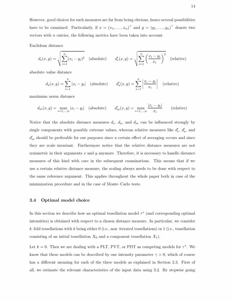
However, good choices for such measures are far from being obvious, hence several possibilities

have to be examined. Particularly, if x = (x1, . . . , xn) and y = (y1, . . . , yn) denote two

vectors with n entries, the following metrics have been taken into account.

Euclidean distance

de(x, y) =

√√√√ n∑i=1

(xi − yi)2 (absolute) d′e(x, y) =

√√√√ n∑i=1

(xi − yi

xi

)2

(relative)

absolute–value distance

da(x, y) =n∑

i=1

|xi − yi| (absolute) d′a(x, y) =n∑

i=1

∣∣∣∣xi − yi

xi

∣∣∣∣ (relative)

maximum–norm distance

dm(x, y) = maxi=1,...,n

|xi − yi| (absolute) d′m(x, y) = maxi=1,...,n

|xi − yi|xi

(relative)

Notice that the absolute distance measures de, da, and dm can be influenced strongly by

single components with possibly extreme values, whereas relative measures like d′e, d′a, and

d′m should be preferable for our purposes since a certain effect of averaging occurs and since

they are scale–invariant. Furthermore notice that the relative distance measures are not

symmetric in their arguments x and y anymore. Therefore, it is necessary to handle distance

measures of this kind with care in the subsequent examinations. This means that if we

use a certain relative distance measure, the scaling always needs to be done with respect to

the same reference argument. This applies throughout the whole paper both in case of the

minimization procedure and in the case of Monte–Carlo tests.

3.4 Optimal model choice

In this section we describe how an optimal tessellation model τ∗ (and corresponding optimal

intensities) is obtained with respect to a chosen distance measure. In particular, we consider

k–fold tessellations with k being either 0 (i.e., non–iterated tessellations) or 1 (i.e., tessellation

consisting of an initial tessellation X0 and a component tessellation X1).

Let k = 0. Then we are dealing with a PLT, PVT, or PDT as competing models for τ∗. We

know that these models can be described by one intensity parameter γ > 0, which of course

has a different meaning for each of the three models as explained in Section 2.3. First of

all, we estimate the relevant characteristics of the input data using 3.2. By stepwise going

15

through a range of intensities for γ and by calculating each time the (theoretical) vector of

characteristics (see Table 1), we finally determine an optimal vector λmin, in the sense that

the distance of the calculated vector of characteristics to the vector of the input characteristics

is minimized. Finally, τ∗ (and also the corresponding optimal intensity γ∗ > 0) is obtained

by minimizing between all tessellation models with respect to the distance d(λ, λmin).

Now, consider the case of k = 1. This means that we consider a 1–fold X0/p X1 Poisson-type

tessellation as described in Section 2.5. In particular, PLT, PVT, and PDT are considered

as models both for X0 and X1. Figures 5 to 7 display examples of all possible choices. Each

of these 1–fold tessellations can be described by two intensity parameters γ0 > 0 and γ1 > 0

as well as the probability p of the Bernoulli–thinning. Again, in the case p = 1, by stepwise

going through a range of intensities for γ0 and for γ1 and by calculating the vector

λ = (λ1, . . . , λ4)

in each step using theoretical formulae (see Table 2), an optimal vector λmin of characteristics

is determined as described above. When we have obtained a vector λmin for each tessellation

model (and therefore a corresponding optimal intensity pair (γ∗0 , γ∗

1)), the overall minimal

value λ∗min is obtained once again by minimizing between all tessellation models with respect

to the distance d(λ, λmin). Hence, the result is a vector λ∗min of characteristics and its

corresponding optimal tessellation model τ∗ with intensity parameters γ∗0 and γ∗

1 . One further

dimension of minimization is introduced if we additionally consider the case p < 1, which

eventually leads to an optimal Bernoulli–thinning parameter p∗.

3.5 Extensions of the decision procedure

To obtain the optimal tessellation model, several extensions of the decision procedure de-

scribed in Section 3.4 are possible. In particular, one can choose ε ≥ 0 in order to obtain the

interval [d∗, d∗(1 + ε)]. Then we would consider every tessellation model to be a candidate

for a possible description of the road system if we obtain an optimal distance value situated

within the interval for this model. Assume we consider a model with obtained optimal dis-

tance, dmin say, where dmin ∈ [d∗, d∗(1 + ε)]. The error for such a model with respect to the

optimal model with distance d∗ is then given by (λmin − λ∗min)/λ∗

min.

16

3.6 Verification of the model choice procedure

The following so–called Monte–Carlo test technique is a general test principle based on sim-

ulations and is widely used in different fields of applications.

We start by establishing a null hypothesis H0 which we want to test. This hypothesis states

that the input data can be described by a certain tessellation model τ(H0), where this model

depends on an intensity parameter γ(H0) in the case of non–iterated tessellations and on

intensity parameters γ0(H0) and γ1(H0) (and possibly a Bernoulli parameter p(H0)) in the

case of nested tessellations.

In order to validate the optimal choice of a tessellation model by the minimization procedure

in Section 3.4, i.e. in order to validate τ∗, we choose τ(H0) = τ∗ and γ(H0) = γ∗ (in case

of non–iterated tessellation models) or γ0(H0) = γ∗0 and γ1(H0) = γ∗

1 (in case of nested

tessellations).

The alternative hypothesis H1 of such a test states that the input data can be described

by the other models that are under consideration. For example if we consider non–iterated

tessellations and if H0 states that τ(H0) = τ∗, where τ∗ is a PLT say, then H1 would state

that the input data can be described by a PVT or a PDT (both with some fixed intensity

parameter which can be obtained through the minimization procedure).

Notice that in case of real input data it is useful not only to test H0 with τ(H0) = τ∗, but

for τ(H0) to go through all tessellation models under consideration. Hence, if τ∗ is a PLT for

example, we also do tests with the second–best and third–best model, i.e. τ(H0) is chosen

to be a a PVT and a PDT for example with some fixed intensity parameters γ(H0).

In what follows, both for the evaluation of the method with simulated data and later on with

real data, we will only state the null hypothesis H0 for short.

Having stated H0, a significance level α has to be chosen, which can be interpreted as the

maximal error to reject H0 despite its correctness. Popular choices are α = 0.05 or α = 0.01.

Subsequently, the tessellation model τ(H0) is simulated n times. Notice that for example

Stoyan and Stoyan (1994) suggest to use n = 99 if α = 0.05 or n = 999 if α = 0.01.

Then, we choose a distance measure and for each simulation we compute the distance between

the estimated vector of the realization of τ(H0) and the vector of characteristics that is

obtained for τ(H0) via theoretical calculation using the intensity parameter γ(H0) (or γ0(H0)

17

and γ1(H0)). Eventually, we obtain n distance values d1, . . . , dn. One further value dn+1 = d∗

is obtained as distance between the vector of characteristics for τ(H0) and the (estimated)

vector of characteristics of input data.

Notice that the distance measure can be chosen independently from the distance measure used

for the minimization procedure. Again, it can be expected that relative distance measures

perform better than absolute ones. However, it has to be pointed out that the order of

the arguments of relative distance measures has to be kept in mind, i.e., complying to the

definition in Section 3.3, the vector of characteristics calculated for γ(H0) (or γ0(H0) and

γ1(H0)) would be the first argument.

Subsequently, the n + 1 values d1, . . . , dn and d∗ are ordered in ascending order, which leads

to a sequence d(1), . . . , d(n+1), where d(i) denotes the ith smallest distance for 1 ≤ i ≤ n + 1.

The null hypothesis H0 is rejected if the position i∗ of d∗ in this ordered sequence is contained

in the rejection region Rα = [n − α(n + 1) + 2, . . . , n + 1]. Alternatively, we may consider

the p–value, which can be expressed as 1− (i∗ − 1)/(n + 1). Notice that this value is always

in the range of [1, 1/(n + 1)]. As always, H0 should be rejected if the obtained p–values are

smaller than the chosen significance level α.

In case of simulated input data the power PMC of Monte–Carlo tests can be estimated and

together with this the probability of the error to accept H0 despite it is not true.

The procedure is in principle analogous to the proceeding described above, except that we

replace τ = τ(H0) by one of the tessellations stated in the alternative hypothesis H1, where

an intensity parameter of τ can be obtained via the minimization procedure. This can be

interpreted in the sense that we examine the performance under H1.

Finally, we repeat the procedure k times, k ≥ 1, and for each = 1, . . . , k we are able to report

whether the position i∗ of the distance d∗ within the ordered sequence d,(1), . . . , d,(n+1) of

distances is in Rα or not. The distance d∗ is calculated between the estimated vector of

characteristics of the input data and the vector of characteristics of the model, which can be

calculated using the theoretical intensity value stated in H1.

Hence, an estimate of the power PMC of the Monte–Carlo test is obtained by regarding the

estimator

PMC =1k

#i∗ ∈ Rα, = 1, . . . , k . (3.4)

18

The power of the Monte–Carlo test can be considered to be high if PMC takes values which

are close to one.

3.7 Numerical examples using simulated data

In the following, we present numerical results, where input data are derived by simulations

of the competing tessellation models. We concentrate on relative distance measures since

simulation studies showed that such distance measures do indeed perform better than absolute

distance measures.

Assume that the input data are realizations of a non–iterated PLT with parameter γ = 0.1

and assume further that we want to verify if our procedure can correctly decide between

a PLT, a PVT, and a PDT. Particularly, the vector λ = (λ1, . . . , λ4) of characteristics as

introduced in (3.1) is considered. Using the vector λ in (3.2) as given by (3.3) as estimator

for the vector of these characteristics, Table 3 shows estimates based on one and on 1000

realizations, respectively, of the input data in a quadratic sampling window of side length

300 (and area 9 × 104). Notice however that in case of the 1000 realizations for example, a

similar quality of estimation can be obtained by only one single realization of the tessellation,

but then in a quadratic sampling window of area 9 × 107.

Table 3: Estimation of characteristics based on n realizations for PLT–input

n = 1 n = 1000 Theoretical

λ1 0.00333 0.00318 0.00318

λ2 0.00611 0.00630 0.00637

λ3 0.00333 0.00318 0.00318

λ4 0.10291 0.09995 0.10000

For the minimization procedure we try to find optimal values for γ within the range [0.0001, 0.5],

where the step width is chosen to be 0.00001. Table 4 displays the numerical values for all

three relative distance measures d′ and the corresponding optimized intensity parameter γ.

For example in the case of the relative Euclidean distance measure d′e, the numerical values

displayed in Table 4 suggest a decision in favor of a PLT as optimal tessellation model τ∗

19

Table 4: Optimal values of d′e, d′

a, and d′m and corresponding optimized parameter γ

d′e,min γ d′a,min γ d′m,min γ

PLT 0.07154 0.10070 0.10112 0.10180 0.04382 0.10010

PVT 0.47164 0.00200 0.76115 0.00200 0.34000 0.00220

PDT 0.62160 0.00180 1.03066 0.00170 0.43816 0.00190

with intensity parameter γ∗ = 0.10070. However, it can be seen that the optimal γ–value is

relatively stable and does not depend strongly on the chosen distance measure.

Table 5: Monte-Carlo test for PLT–input, where τ (H0) is a PLT with γ = 0.10070

α n Rα d∗ d(1) d(n+1) i∗ p–value reject

0.05 99 [96, 100] 0.00223 0.00011 0.04312 8 0.93 no

0.01 999 [991, 1000] 0.00223 0.00015 0.07141 108 0.893 no

Table 5 displays the results of a Monte–Carlo test, where the null hypothesis H0 states that

τ(H0) = τ∗, i.e. H0 states that the input data can be represented by a PLT with intensity

γ(H0) = γ∗ = 0.10070. The distances are calculated using the relative Euclidean distance. To

get an impression of the range of the ascending ordered sequence of distances d(1), . . . , d(n+1),

the values d(1) and d(n+1) are displayed in Table 5. Furthermore, the position i∗ of d∗ within

this ordered sequence of distances is given. The decision to not reject the null hypothesis can

be obtained via two approaches. First, we see that i∗ /∈ Rα. Second, the p–values are very

large overall and also compared to the significance levels α = 5% and α = 1%. Therefore,

H0 is not rejected and hence we may say that the input data can be represented by a PLT

with intensity parameter 0.1007.

Finally, we examine the power PMC of this Monte–Carlo test. Hence, we proceed as described

in Section 3.6 and replace in the simulations the PLT model by the models stated in the

alternative hypothesis H1, namely by a PVT (with some optimal intensity parameter) and

by a PDT (with some optimal intensity parameter). We choose k = 1000, i.e. the whole

procedure of estimating the power using the estimator PMC in (3.4) is repeated 1000 times.

20

In case of a PVT and a significance level α = 0.05, Table 6 shows the results of one of the

1000 repetitions, and as estimated power we obtain the value PMC = 1. The same result is

Table 6: Power examination for PLT–input with simulated PVT

α n Rα d∗ d(1) d(n+1) i∗

0.05 99 [96, 100] 0.01355 0.00004 0.01355 100

0.01 999 [991, 1000] 0.01355 0.00005 0.01355 1000

obtained for the case of a PDT with intensity γ = 0.00180 (again for α = 0.05).

Notice that this rather high estimated value for power can be explained by the fact that PLT

on one side and both PVT and PDT on the other side are quite different models with regard

to their geometrical structure.

As a second example the input data are now derived from a X0/p X1–tessellation, where

X0 and X1 are chosen to be a PLT with parameter γ1 = 0.08 and a PDT with parameter

γ2 = 0.0008, respectively. In the case of p = 1 we obtain 9 competing models. Additionally

we can consider the case where p is any arbitrary number with 0 ≤ p < 1. Notice however,

that such a minimization increases the computational complexity remarkably. Therefore, we

first concentrate on the case p = 1, which is interesting in its own right due to a certain

symmetry inherent in the intensity formulae shown in Table 2.

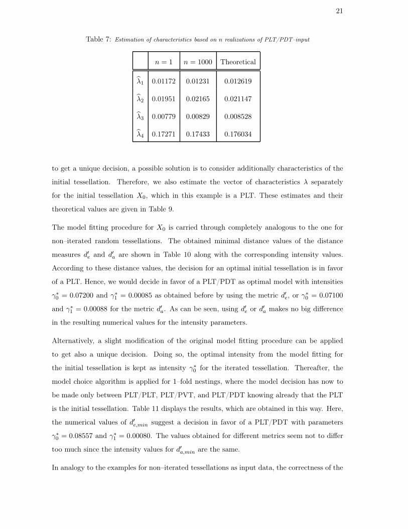
Again the same vector λ1, . . . , λ4 of characteristics given in (3.1) is considered. Table 7,

which can be understood completely analogously to Table 3, shows the performance of our

estimators, based on one and on 1000 sample realizations of the PLT/PDT–tessellation,

respectively.

For the minimization procedure we try to find optimal values for γ0 and γ1 within the

range [0.00001, 0.15], where the step width is chosen to be 0.00001. As distance measures

the relative Euclidean metric d′e and the relative absolute–value metric d′a are considered.

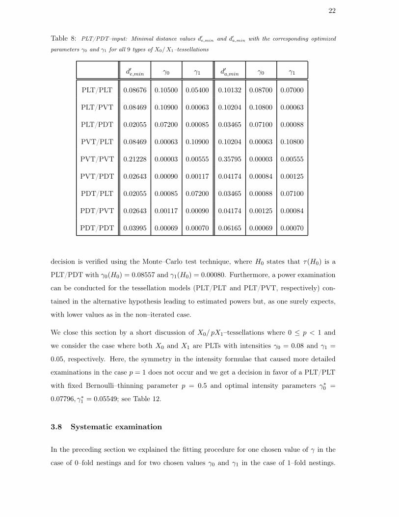
For the alternative measure d′m similar results are obtained. Table 8 displays the minimal

distance values d′e,min and d′a,min of d′e and d′a, respectively, for each tessellation model and the

corresponding optimized intensity parameters γ0 and γ1. Minimizing the obtained distance

values over all nine possible tessellation models, the decision is in favor of a PLT/PDT or a

PDT/PLT and hence, due the symmetry explained above, is not unique. However, in order

21

Table 7: Estimation of characteristics based on n realizations of PLT/PDT–input

n = 1 n = 1000 Theoretical

λ1 0.01172 0.01231 0.012619

λ2 0.01951 0.02165 0.021147

λ3 0.00779 0.00829 0.008528

λ4 0.17271 0.17433 0.176034

to get a unique decision, a possible solution is to consider additionally characteristics of the

initial tessellation. Therefore, we also estimate the vector of characteristics λ separately

for the initial tessellation X0, which in this example is a PLT. These estimates and their

theoretical values are given in Table 9.

The model fitting procedure for X0 is carried through completely analogous to the one for

non–iterated random tessellations. The obtained minimal distance values of the distance

measures d′e and d′a are shown in Table 10 along with the corresponding intensity values.

According to these distance values, the decision for an optimal initial tessellation is in favor

of a PLT. Hence, we would decide in favor of a PLT/PDT as optimal model with intensities

γ∗0 = 0.07200 and γ∗

1 = 0.00085 as obtained before by using the metric d′e, or γ∗0 = 0.07100

and γ∗1 = 0.00088 for the metric d′a. As can be seen, using d′e or d′a makes no big difference

in the resulting numerical values for the intensity parameters.

Alternatively, a slight modification of the original model fitting procedure can be applied

to get also a unique decision. Doing so, the optimal intensity from the model fitting for

the initial tessellation is kept as intensity γ∗0 for the iterated tessellation. Thereafter, the

model choice algorithm is applied for 1–fold nestings, where the model decision has now to

be made only between PLT/PLT, PLT/PVT, and PLT/PDT knowing already that the PLT

is the initial tessellation. Table 11 displays the results, which are obtained in this way. Here,

the numerical values of d′e,min suggest a decision in favor of a PLT/PDT with parameters

γ∗0 = 0.08557 and γ∗

1 = 0.00080. The values obtained for different metrics seem not to differ

too much since the intensity values for d′a,min are the same.

In analogy to the examples for non–iterated tessellations as input data, the correctness of the

22

Table 8: PLT/PDT–input: Minimal distance values d′e,min and d′

a,min with the corresponding optimized

parameters γ0 and γ1 for all 9 types of X0/ X1–tessellations

d′e,min γ0 γ1 d′a,min γ0 γ1

PLT/PLT 0.08676 0.10500 0.05400 0.10132 0.08700 0.07000

PLT/PVT 0.08469 0.10900 0.00063 0.10204 0.10800 0.00063

PLT/PDT 0.02055 0.07200 0.00085 0.03465 0.07100 0.00088

PVT/PLT 0.08469 0.00063 0.10900 0.10204 0.00063 0.10800

PVT/PVT 0.21228 0.00003 0.00555 0.35795 0.00003 0.00555

PVT/PDT 0.02643 0.00090 0.00117 0.04174 0.00084 0.00125

PDT/PLT 0.02055 0.00085 0.07200 0.03465 0.00088 0.07100

PDT/PVT 0.02643 0.00117 0.00090 0.04174 0.00125 0.00084

PDT/PDT 0.03995 0.00069 0.00070 0.06165 0.00069 0.00070

decision is verified using the Monte–Carlo test technique, where H0 states that τ(H0) is a

PLT/PDT with γ0(H0) = 0.08557 and γ1(H0) = 0.00080. Furthermore, a power examination

can be conducted for the tessellation models (PLT/PLT and PLT/PVT, respectively) con-

tained in the alternative hypothesis leading to estimated powers but, as one surely expects,

with lower values as in the non–iterated case.

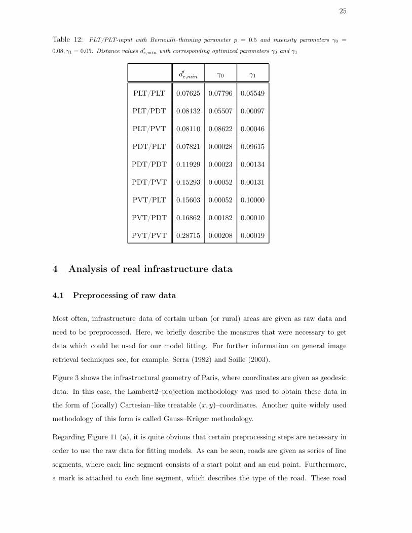
We close this section by a short discussion of X0/ pX1–tessellations where 0 ≤ p < 1 and

we consider the case where both X0 and X1 are PLTs with intensities γ0 = 0.08 and γ1 =

0.05, respectively. Here, the symmetry in the intensity formulae that caused more detailed

examinations in the case p = 1 does not occur and we get a decision in favor of a PLT/PLT

with fixed Bernoulli–thinning parameter p = 0.5 and optimal intensity parameters γ∗0 =

0.07796, γ∗1 = 0.05549; see Table 12.

3.8 Systematic examination

In the preceding section we explained the fitting procedure for one chosen value of γ in the

case of 0–fold nestings and for two chosen values γ0 and γ1 in the case of 1–fold nestings.

23

Table 9: Estimation of characteristics of n realization of the initial tessellation of the PLT/PDT–tessellation

n = 1 n = 1000 Theoretical

λ1 0.00232 0.00206 0.00204

λ2 0.00464 0.00411 0.00407

λ3 0.00232 0.00206 0.00204

λ4 0.08754 0.08033 0.08000

Table 10: Initial tessellation of PLT/PDT: Distance values d′e,min and d′

a,min with corresponding optimized

parameter γ for PLT, PVT, and PDT

d′e,min γ d′a,min γ

PLT 0.02338 0.08557 0.02458 0.08541

PVT 0.47263 0.00147 0.76779 0.00155

PDT 0.62622 0.00128 1.07166 0.00116

The intention of this section is to show that our procedure of course works correctly not only

for these choices but also for other numerical values of intensity parameters. We constraint

ourselves to present a systematic examination in the case of simple tessellations.

We consider input data derived from a PLT with intensity parameter γ ∈ [0.01, 0.3]. The

step width is 0.001 for 0.01 ≤ γ ≤ 0.05 and step width 0.01 for 0.05 ≤ γ ≤ 0.3. Notice that

the sampling window for the simulations is again a rectangle with side length 300.

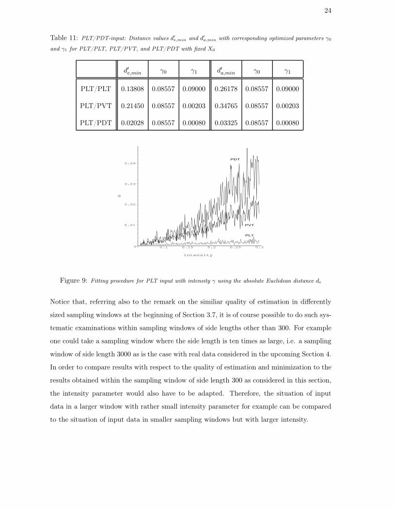
Figure 9 shows the results of the examination of our fitting procedure where the absolute

Euclidean distance de was used. We observe that overall the PLT is indeed recognized as best

model, however the distinction between the models gets better and better with increasing

intensity γ. In contrast to that we see the same result with the relative Euclidean distance d′e

in Figure 10. There, the distances between the optimal model (PLT) and its two alternatives

is quite larger than in case of the absolute distance. Moreover, the quality of distinction is

the same for each value of γ.

24

Table 11: PLT/PDT-input: Distance values d′e,min and d′

a,min with corresponding optimized parameters γ0

and γ1 for PLT/PLT, PLT/PVT, and PLT/PDT with fixed X0

d′e,min γ0 γ1 d′a,min γ0 γ1

PLT/PLT 0.13808 0.08557 0.09000 0.26178 0.08557 0.09000

PLT/PVT 0.21450 0.08557 0.00203 0.34765 0.08557 0.00203

PLT/PDT 0.02028 0.08557 0.00080 0.03325 0.08557 0.00080

PDT

PVT

PLT

0

0.01

0.02

0.03

0.04

d

0.1 0.15 0.2 0.25 0.3

intensity

Figure 9: Fitting procedure for PLT input with intensity γ using the absolute Euclidean distance de

Notice that, referring also to the remark on the similiar quality of estimation in differently

sized sampling windows at the beginning of Section 3.7, it is of course possible to do such sys-

tematic examinations within sampling windows of side lengths other than 300. For example

one could take a sampling window where the side length is ten times as large, i.e. a sampling

window of side length 3000 as is the case with real data considered in the upcoming Section 4.

In order to compare results with respect to the quality of estimation and minimization to the

results obtained within the sampling window of side length 300 as considered in this section,

the intensity parameter would also have to be adapted. Therefore, the situation of input

data in a larger window with rather small intensity parameter for example can be compared

to the situation of input data in smaller sampling windows but with larger intensity.

25

Table 12: PLT/PLT-input with Bernoulli–thinning parameter p = 0.5 and intensity parameters γ0 =

0.08, γ1 = 0.05: Distance values d′e,min with corresponding optimized parameters γ0 and γ1

d′e,min γ0 γ1

PLT/PLT 0.07625 0.07796 0.05549

PLT/PDT 0.08132 0.05507 0.00097

PLT/PVT 0.08110 0.08622 0.00046

PDT/PLT 0.07821 0.00028 0.09615

PDT/PDT 0.11929 0.00023 0.00134

PDT/PVT 0.15293 0.00052 0.00131

PVT/PLT 0.15603 0.00052 0.10000

PVT/PDT 0.16862 0.00182 0.00010

PVT/PVT 0.28715 0.00208 0.00019

4 Analysis of real infrastructure data

4.1 Preprocessing of raw data

Most often, infrastructure data of certain urban (or rural) areas are given as raw data and

need to be preprocessed. Here, we briefly describe the measures that were necessary to get

data which could be used for our model fitting. For further information on general image

retrieval techniques see, for example, Serra (1982) and Soille (2003).

Figure 3 shows the infrastructural geometry of Paris, where coordinates are given as geodesic

data. In this case, the Lambert2–projection methodology was used to obtain these data in

the form of (locally) Cartesian–like treatable (x, y)–coordinates. Another quite widely used

methodology of this form is called Gauss–Krüger methodology.

Regarding Figure 11 (a), it is quite obvious that certain preprocessing steps are necessary in

order to use the raw data for fitting models. As can be seen, roads are given as series of line

segments, where each line segment consists of a start point and an end point. Furthermore,

a mark is attached to each line segment, which describes the type of the road. These road

26

PDT

PVT

PLT

0

0.1

0.2

0.3

0.4

0.5

0.6

0.7

d

0.05 0.1 0.15 0.2 0.25 0.3

intensity

Figure 10: Fitting procedure for PLT input with intensity γ using the relative Euclidean distance d′e

types rank from highways and national routes down to small side streets. In our analysis,

we concentrate on only two types, which we identified to be the most common road types

in Paris, namely intercity main roads and side streets. Finally, we remove dead end streets

and by traversing through the line segments it is possible to reconstruct a tessellation which

consists of polygonal cells; Figure 11 (b). Still however, points may exist, which do not belong

to the set of vertices of the obtained tessellation. Clearly, these are points where only two

line segments emanate from and therefore it is easy to not account for such points.

4.2 Numerical results

We examine preprocessed data of Paris within a rectangular sampling window W ; see Fig-

ure 12. Since in our case we know how to differentiate between main roads and side streets,

our philosophy is to use 1–fold tessellation models for data fitting. Hence we expect to get

a realistic and adequate model for our data, since we additionally use the information about

their hierarchical structure.

We restrict our description to the case of X0/p X1–tessellations where p = 1. As pointed out

earlier, this is a rather complicated case since the decision is not unique from the first and

we have to use some more information to get a unique decision. Notice that in the case of

p < 1 the decision is unique. Minimization of an additional parameter p however is little

more challenging regarding the computational run times.

We start by considering the main roads contained in Figure 12. Table 13 shows results of

27

(a) Extracted data (b) Preprocessed data

Figure 11: Infrastructure of Paris. From raw data to preprocessed data

the minimization procedure applied to the main road data if we use the relative Euclidean

metric d′e as a measure of distance. Here the decision would be in favor of a PLT, i.e. τ∗

is a PLT with optimal intensity parameter γ∗ = 0.002384. However, regarding the distance

values and using the alternative decision rule of Section 3.5 with ε = 0.5 for example, we

cannot rule out a PVT with intensity parameter γ = 0.000001.

Table 13: Main road input data of Figure 12: Distance values d′e,min and corresponding optimized parameter

γ for PLT, PVT, and PDT

X d′e,min γ∗

PLT 0.21101 0.002384

PVT 0.29749 0.000001

PDT 0.73378 0.000001

As far as Monte–Carlo tests are concerned for real data input, the idea is to do these tests

for all considered tessellation models and to check whether a certain model can be taken as

representation of the real data. In the case of X0 for example, we consider null hypotheses H0

for non–iterated tessellations, i.e. τ(H0) is chosen to be, one at a time, PLT, PVT, and PDT

with intensity parameter γ(H0). Hence, Table 14, Table 15, and Table 16 show the results

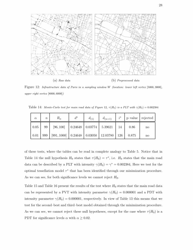
28

(a) Raw data (b) Preprocessed data

Figure 12: Infrastructure data of Paris in a sampling window W (location: lower left vertex [5000, 3000],

upper right vertex [8000, 6000])

Table 14: Monte-Carlo test for main road data of Figure 12, τ (H0) is a PLT with γ(H0) = 0.002384

α n Rα d∗ d(1) d(n+1) i∗ p–value rejected

0.05 99 [96, 100] 0.24648 0.03774 5.39621 14 0.86 no

0.01 999 [991, 1000] 0.24648 0.03050 12.03780 126 0.875 no

of these tests, where the tables can be read in complete analogy to Table 5. Notice that in

Table 14 the null hypothesis H0 states that τ(H0) = τ∗, i.e. H0 states that the main road

data can be described by a PLT with intensity γ(H0) = γ∗ = 0.002384, Here we test for the

optimal tessellation model τ∗ that has been identified through our minimization procedure.

As we can see, for both significance levels we cannot reject H0.

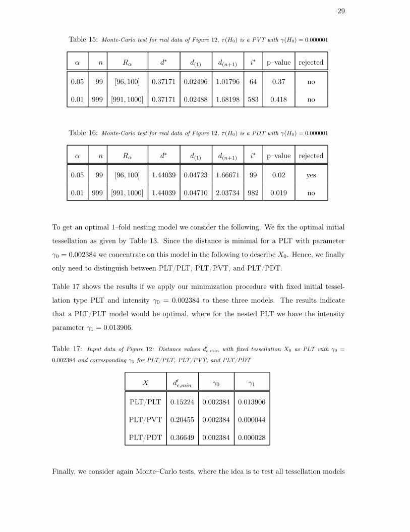
Table 15 and Table 16 present the results of the test where H0 states that the main road data

can be represented by a PVT with intensity parameter γ(H0) = 0.000001 and a PDT with

intensity parameter γ(H0) = 0.000001, respectively. In view of Table 13 this means that we

test for the second–best and third–best model obtained through the minimization procedure.

As we can see, we cannot reject these null hypotheses, except for the case where τ(H0) is a

PDT for significance levels α with α ≥ 0.02.

29

Table 15: Monte-Carlo test for real data of Figure 12, τ (H0) is a PVT with γ(H0) = 0.000001

α n Rα d∗ d(1) d(n+1) i∗ p–value rejected

0.05 99 [96, 100] 0.37171 0.02496 1.01796 64 0.37 no

0.01 999 [991, 1000] 0.37171 0.02488 1.68198 583 0.418 no

Table 16: Monte-Carlo test for real data of Figure 12, τ (H0) is a PDT with γ(H0) = 0.000001

α n Rα d∗ d(1) d(n+1) i∗ p–value rejected

0.05 99 [96, 100] 1.44039 0.04723 1.66671 99 0.02 yes

0.01 999 [991, 1000] 1.44039 0.04710 2.03734 982 0.019 no

To get an optimal 1–fold nesting model we consider the following. We fix the optimal initial

tessellation as given by Table 13. Since the distance is minimal for a PLT with parameter

γ0 = 0.002384 we concentrate on this model in the following to describe X0. Hence, we finally

only need to distinguish between PLT/PLT, PLT/PVT, and PLT/PDT.

Table 17 shows the results if we apply our minimization procedure with fixed initial tessel-

lation type PLT and intensity γ0 = 0.002384 to these three models. The results indicate

that a PLT/PLT model would be optimal, where for the nested PLT we have the intensity

parameter γ1 = 0.013906.

Table 17: Input data of Figure 12: Distance values d′e,min with fixed tessellation X0 as PLT with γ0 =

0.002384 and corresponding γ1 for PLT/PLT, PLT/PVT, and PLT/PDT

X d′e,min γ0 γ1

PLT/PLT 0.15224 0.002384 0.013906

PLT/PVT 0.20455 0.002384 0.000044

PLT/PDT 0.36649 0.002384 0.000028

Finally, we consider again Monte–Carlo tests, where the idea is to test all tessellation models

30

given in Table 17, i.e. for H0 we choose τ(H0) to be a PLT/PLT, PLT/PVT, or PLT/PDT

with intensity parameters γ0(H0) = γ0 and γ1(H0) = γ1, respectively, as given in Table 17.

We restrict ourselves to two examples. First we consider the case where H0 states that

τ(H0) is a PLT/PDT with intensity parameters γ0(H0) = 0.002384 and γ1(H0) = 0.000028.

Table 18 and Table 19 show the results both for the case of the relative Euclidean dis-

tance (Table 18) and for the case of the absolute Euclidean distance (Table 19), respectively.

Regarding Table 18, we see that with the relative Euclidean distance we would not reject the

Table 18: Monte-Carlo test for real data of Figure 12, τ (H0) is a PLT/PDT with γ0(H0) = 0.002384 and

γ1(H0) = 0.000028 (relative Euclidean distance)

α n Rα d∗ d(1) d(n+1) i∗ p–value rejected

0.05 99 [96, 100] 0.43747 0.01339 1.28781 83 0.18 no

0.01 999 [991, 1000] 0.43747 0.00460 1.16786 816 0.185 no

null hypothesis, however regarding the rank i∗ of d∗ in the ordered sequence of distances (and

hence regarding the p–value), this decision is relatively tight. Using however the absolute

Euclidean distance for the same test, we conclude that the null hypothesis has to be rejected.

Similar tests can also be done for the case where H0 states that γ(H0) is a PLT/PVT type

Table 19: Monte-Carlo test for real data of Figure 12, τ (H0) is a PLT/PDT with γ0(H0) = 0.002384 and

γ1(H0) = 0.000028 (absolute Euclidean distance)

α n Rα d∗ d(1) d(n+1) i∗ p–value rejected

0.05 99 [96, 100] 0.00313 0.00003 0.00313 100 0.00 yes

0.01 999 [991, 1000] 0.00313 1.15251 0.00355 997 0.004 yes

tessellation.

Finally, Table 20 shows the results of the Monte–Carlo test for the null hypothesis H0 with

τ(H0) = τ∗ and τ∗ being a PLT/PLT as obtained according to the minimization procedure

with optimal intensity parameters γ∗0 = 0.002384 and γ∗

1 = 0.013906. In this case, using the

relative Euclidean distance, we cannot reject this null hypothesis. We also considered this

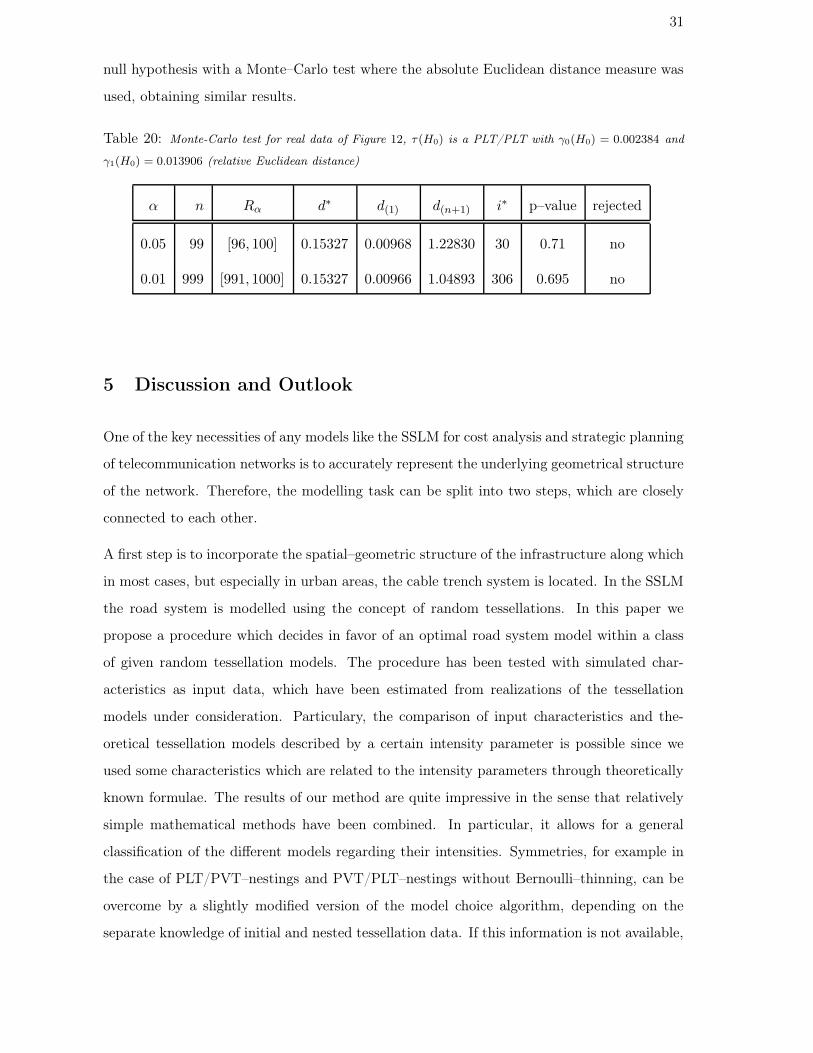
31

null hypothesis with a Monte–Carlo test where the absolute Euclidean distance measure was

used, obtaining similar results.

Table 20: Monte-Carlo test for real data of Figure 12, τ (H0) is a PLT/PLT with γ0(H0) = 0.002384 and

γ1(H0) = 0.013906 (relative Euclidean distance)

α n Rα d∗ d(1) d(n+1) i∗ p–value rejected

0.05 99 [96, 100] 0.15327 0.00968 1.22830 30 0.71 no

0.01 999 [991, 1000] 0.15327 0.00966 1.04893 306 0.695 no

5 Discussion and Outlook

One of the key necessities of any models like the SSLM for cost analysis and strategic planning

of telecommunication networks is to accurately represent the underlying geometrical structure

of the network. Therefore, the modelling task can be split into two steps, which are closely

connected to each other.

A first step is to incorporate the spatial–geometric structure of the infrastructure along which

in most cases, but especially in urban areas, the cable trench system is located. In the SSLM

the road system is modelled using the concept of random tessellations. In this paper we

propose a procedure which decides in favor of an optimal road system model within a class

of given random tessellation models. The procedure has been tested with simulated char-

acteristics as input data, which have been estimated from realizations of the tessellation

models under consideration. Particulary, the comparison of input characteristics and the-

oretical tessellation models described by a certain intensity parameter is possible since we

used some characteristics which are related to the intensity parameters through theoretically

known formulae. The results of our method are quite impressive in the sense that relatively

simple mathematical methods have been combined. In particular, it allows for a general

classification of the different models regarding their intensities. Symmetries, for example in

the case of PLT/PVT–nestings and PVT/PLT–nestings without Bernoulli–thinning, can be

overcome by a slightly modified version of the model choice algorithm, depending on the

separate knowledge of initial and nested tessellation data. If this information is not available,

32

i.e., if we cannot distinguish between initial and nested tessellation in a 1–fold nesting say,

then it might be a good idea to choose some small ε > 0 and fit an X0/p X1–nesting with

p = 1−ε. Hence, the decision is unique and letting ε → 0, i.e. executing a sequence of fitting

steps with ε getting smaller and smaller, the hope is that also the decision for the limiting

tessellation is in favor of that same X0/p X1–nesting.

Finally, the model choice procedure has been confronted with a set of (preprocessed) infra-

structure data of Paris. Owing to the structure of the data, which clearly do not follow any of

the proposed tessellation models, the fit is worse, but still relatively impressive regarding our

numerical results. Naturally, we can only hope to identify one model among the theoretically

proposed which comes closest to the given data.

Clearly, it is necessary to refine the fitting procedure. One possibility can be the application

of central limit theorems, like in Heinrich, Schmidt and Schmidt (2005). There, asymptotical

studies of the distribution of certain functionals of both Poisson line tessellations as well

as Poisson–Voronoi tessellations are shown, where the asymptotic comes in through an un-

boundedly growing sampling window. Such results lead to central limit theorems and hence

to (asymptotic) confidence intervals and tests.

In a second step, the chosen geometric model representation of the infrastructure has to

be used for evaluation of the network. Therefore, the network equipment is placed onto the

chosen tessellation model for the road system. Realizations of certain types of point processes

are used to represent these nodes. In particular, one is interested in the tree connecting

subscribers of a certain serving area to the corresponding WCS–station via intermediate

stations of lower level along the road system. Routing techniques can be applied to analyze

shortest paths between subscribers and equipment of any hierarchy level in the network. For

example, the expected mean of shortest path lengths between a WCS–station and a SAI–

station can be examined for random tessellation models. This will lead to simulated results

or even theoretical formulae for the whole tree connecting subscribers of a certain serving

zone to the corresponding WCS–station. Further information can be found in Gloaguen et

al. (2005a, 2005b), where we present simulation techniques and results using simulation of

typical cells, corresponding typical trees, and reduction of parameters through parametric

scaling.

33

Acknowledgement

This research was supported by France Télécom through research grant 42 36 68 97. The

authors are grateful to Simone Hörner and Stefanie Eckel for their help in performing the

large–scale simulations, which led to the numerical results. Also, valuable comments of two

anonymous referees are gratefully acknowledged.

34

References

[1] F. Baccelli and B. Blaszczyszyn. (2001). “On a coverage process ranging from the Booleanmodel to the Poisson-Voronoi tessellation.” Advances in Applied Probability 33, 293–323.

[2] F. Baccelli, C. Gloaguen, and S. Zuyev. (2000). “Superposition of Planar Voronoi Tes-sellations.” Communications in Statistics, Series Stochastic Models 16, 69–98.

[3] F. Baccelli, M. Klein, M. Lebourges, and S. Zuyev. (1996). “Géomètrie aléatoire etarchitecture de réseaux.” Annales des Télécommunication 51, 158–179.

[4] F. Baccelli, D. Kofman, and J.L. Rougier. (1999). “Self organizing hierarchical multicasttrees and their optimization.” Proceedings of IEEE Infocom ’99, 1081–1089, New York.

[5] F. Baccelli and S. Zuyev. (1996). “Poisson-Voronoi spanning trees with applications tothe optimization of communication networks.” Operations Research 47, 619–631.

[6] A.J. Baddeley and E.B. Vedel Jensen. (2004). Stereology for Statisticians. Chapman &Hall.

[7] C. Gloaguen, P. Coupé, R. Maier and V. Schmidt. (2002). “Stochastic modelling of urbanaccess networks.” Proc. 10th Internat. Telecommun. Network Strategy Planning Symp.,(Munich, June 2002), VDE, Berlin, pp. 99-104.

[8] C. Gloaguen, F. Fleischer, H. Schmidt and V. Schmidt. (2005a). “Simulation of typicalCox-Voronoi cells, with a special regard to implementation tests.” Mathematical Methodsof Operations Research 62, to appear.

[9] C. Gloaguen, F. Fleischer, H. Schmidt and V. Schmidt. (2005b). “Analysis of shortestpaths and subscriber line lengths in telecommunication access networks.” Working paper,under preparation.

[10] L. Heinrich, H. Schmidt and V. Schmidt (2005). “Central Limit Theorems for PoissonHyperplane Tessellations”. Preprint, submitted.

[11] R. Maier. (2003). Iterated Random Tessellations with Applications in Spatial Modellingof Telecommunication Networks. Doctoral Dissertation, University of Ulm.

[12] R. Maier, J. Mayer and V. Schmidt. (2004). “Distributional properties of the typical cellof stationary iterated tessellations.” Mathematical Methods of Operations Research 59,287–302.

[13] R. Maier and V. Schmidt. (2003). “Stationary iterated tessellations.” Advances in AppliedProbability 35, 337–353.

[14] J. Mayer, V. Schmidt and F. Schweiggert. (2004). “A unified simulation framework forspatial stochastic models.” Simulation Modelling Practice and Theory 12, 307–326.

[15] J. Møller. (1989). “Random tessellations in IRd.” Advances in Applied Probability 21,37–73.

[16] J. Ohser and F. Mücklich. (2000). Statistical Analysis of Microstructures in MaterialsScience. J.Wiley & Sons, Chichester.

35

[17] A. Okabe, B. Boots, K. Sugihara and S.N. Chiu. (2000). Spatial Tessellations. 2nd ed.,J.Wiley & Sons, Chichester.

[18] R. Schneider and W. Weil. (2000). Stochastische Geometrie. Teubner, Stuttgart.

[19] J. Serra. (1982). Image Analysis and Mathematical Morphology. Academic Press, London.

[20] P. Soille. (2003). Morphological Image Analysis. Springer, Berlin.

[21] D. Stoyan, W.S. Kendall and J. Mecke. (1995). Stochastic Geometry and its Applications.2nd ed., J. Wiley & Sons, Chichester.

[22] D. Stoyan and H. Stoyan. (1994). Fractals, Random Shapes and Point Fields. Methodsof Geometrical Statistics. J.Wiley & Sons, Chichester.

[23] K. Tchoumatchenko and S. Zuyev. (2001). “Aggregate and fractal tessellations.” Proba-bility Theory Related Fields 121, 198–218.

36

37

Footnotes

Affiliation of authors

Dr. Catherine GLOAGUENFrance Telecom R&D Division RESA/NET/NSO, 92794 Issy Moulineaux Cedex 9, France

Dipl.-Math. oec. Frank FLEISCHER M.Sc.Department of Applied Information Processing and Department of Stochastics, University ofUlm, 89069 Ulm, Germany

Dipl.-Math. oec. Hendrik SCHMIDT M.Sc.Department of Stochastics, University of Ulm, 89069 Ulm, Germany

Professor Volker SCHMIDTDepartment of Stochastics, University of Ulm, 89069 Ulm, Germany

38

Contact author

Catherine GLOAGUEN

France Télécom R&D RESA/NET/NSO

38-40 Rue du Général Leclerc

92794 Issy Moulineaux Cedex 9, France

E-mail : [email protected]

Tel : + 33 1 45 29 64 41

Fax : + 33 1 45 29 63 07

39

Keywords

Telecommunication network modelling

Stochastic geometry

Access network

Random tessellations

Statistical fitting

Monte–Carlo tests

40

Manuscript Dates

Submission : December, 20th, 2004

First revision : June, 24th, 2005

Second revision : October, 7th, 2005