Enhancing democracy through legislative redistricting

Enhancing Democracy Through Legislative Redistricting

(Article begins on next page)

The Harvard community has made this article openly available.Please share how this access benefits you. Your story matters.

Citation Gelman, Andrew, and Gary King. 1994. Enhancing democracythrough legislative redistricting. American Political Science Review88(3): 541-559.

Published Version doi:10.2307/2944794

Accessed February 26, 2013 10:49:19 PM EST

Citable Link http://nrs.harvard.edu/urn-3:HUL.InstRepos:4266310

Terms of Use This article was downloaded from Harvard University's DASHrepository, and is made available under the terms and conditionsapplicable to Other Posted Material, as set forth athttp://nrs.harvard.edu/urn-3:HUL.InstRepos:dash.current.terms-of-use#LAA

http://osc.hul.harvard.edu/dash/open-access-feedback?handle=1/4266310&title=Enhancing+Democracy+Through+Legislative+Redistricting

http://dx.doi.org/10.2307/2944794

http://nrs.harvard.edu/urn-3:HUL.InstRepos:4266310

http://nrs.harvard.edu/urn-3:HUL.InstRepos:dash.current.terms-of-use#LAA

http://nrs.harvard.edu/urn-3:HUL.InstRepos:dash.current.terms-of-use#LAA

American Political Science Review Vol. 88, No. 3 September 1994

ENHANCING DEMOCRACY THROUGH LEGISLATIVE REDISTRICTING ANDREW GELMAN University of California, Berkeley GARY KING Haward University

e demonstrate the surprising benefits of legislative redistricting (including partisan gerrymandering) for American representative democracy. In so doing, our analysis resolves two long-standing controversies in American politics. First, whereas some w

scholars believe that redistricting reduces electoral responsiveness by protecting incumbents, others, that the relationship is spurious, we demonstrate that both sides are wrong: redistricting increases responsiveness. Second, while some researchers believe that gerrymandering dramatically increases partisan bias and others deny this effect, we show both sides are in a sense correct. Gerrymandering biases electoral systems in favor of the party that controls the redistricting as compared to what would have happened if the other party controlled it, but any type of redistricting reduces partisan bias as compared to an electoral system without redistricting. Incorrect conclusions in both literatures resulted from misjudging the enormous uncertainties present during redistricting periods, making simplified assumptions about the redistricters' goals, and using inferior statistical methods.

I n 1982, the Michigan Supreme Court imposed a redistricting plan on their state that was generally believed to favor the Republicans. The Democrats'

alternative measure had to pass the legislature with a two-thirds vote, which was difficult even though they had a majority in both houses. Democratic leaders tried to sneak through the legislation by gutting the contents, but not the title, of an irrelevant bill at the last minute and inserting redistricting legislation. The Republicans discovered this ploy, making the situation extremely tense. In the heat of the long debate during this midnight session, a Democratic senator collapsed. Paramedics were called in, but he refused to leave the Senate floor before the vote. In a classic case of political hardball, a Republican senator used parliamentary procedure to delay the vote by insist- ing that the legal description of all 148 legislative districts and their boundaries be read into the record. Despite his failing health, the Democratic senator stayed through the entire reading, and his party won the vote.'

During the Illinois redistricting process,

Republican state Senator Mark Rhoads believed he had the Democratic votes needed to pass a GOP map in the Senate. In a rare Sunday legislative session Rhoads became outraged over the parliamentary tactics em- ployed by [Senator] Rock to delay a vote on reapportionment. Unable to control his anger, Rhoads attempted to charge the podium and get at Rock. However, before he reached the burly Senate president, Democratic down- state Senator Sam Vadalabene sucker-punched Rhoads with a right to the jaw. According to eyewitness A1 Manning of the State Journal Register, "for a moment it looked as though both benches were going to empty," but, with the television cameras grinding, the combat- ants were pulled apart. Later in the day, Rock eventually called the remap bill and with total party unity the Democrats passed out their own bill, thus assuring a reapportionment deadlock. (Green 1982, 32)

These are among the most colorful recent redistricting stories, but they accurately portray the intensity of the partisan conflict in many such processes throughout the United States. From George Wash- ington's first presidential veto to the present day, redistricting issues have been extremely controversial at every level of government. Most redistrictings are contested in state and federal court cases heard so late that there is insufficient time to follow the usual rules of discovery, evidence, or due process. In total, legislative redistricting is one of the most conflictual forms of regular politics in the United States short of violence.

While partisan and bipartisan redistricting plans can protect incumbents, they only protect some of those who survive the redistricting process-and many do not survive. Indeed, most incumbent politicians would give an awful lot to avoid redistricting altogether. After all, they are fighting over the fun- damental rules of the game (fights that might well have been concluded at the founding of the republic) and for their own political survival. As a result, redistricting creates enormous levels of uncertainty, an extremely undesirable situation for any sitting politician. Indeed, because the costs of the political fight frequently outweigh the benefits of government service during redistricting, incumbents dispropor- tionately choose to retire at this time.'

Some scholars assume that those who draw the district lines are motivated by incumbent protection, whereas others believe the motivation is partisan advantage, but even the briefest discussion with participants in the process indicates that redistricters are concerned with both. Indeed, these are often competing goals: incumbents are often forced to give up votes (hence electoral safety) in order to increase the number of legislative seats their party is likely to capture. The tension between the goals of individual and partisan advantage creates yet additional uncer-

Legislative Redistricting September 1994

tainty about the outcome of a redistricting. Since political party gain is the most predictable common ground for otherwise competing incumbents, party advantage will often take precedence over individual incumbents' advantage in the ultimate political compromise represented by a redistricting plan.

Moreover, not only do redistricters attempt to maximize the competing goals of incumbency protection and partisan advantage, but incumbency protection is itself composed of competing goals: winning the general election and winning (or avoiding) the primary election. These goals conflict because adding too many of a legislator's political party members to his or her district (hence piling up expected votes in the general election) might leave the incumbent vul- nerable to a now larger opposition faction within his or her party primary.3

In addition to the high levels of political conflict and uncertainty and the conflicting goals of those who draw the district lines, the entire process in- cludes several severe legal and political constraints. These include the requirements of equal population, contiguity, compactness, minority representation, maintaining communities of interest, not splitting local subdivisions, and especially protecting some incumbents, all within the context of complicated local geography. Other constraints are much less widely recognized but no less important to incumbents, such as the inclusion of the right political contributors, the exclusion of prospective challeng- ers, and the keeping of each favored incumbent's several district offices within the di~tr ic t .~

Thus, in our view, the key to understanding the effects of redistricting is to view redistricters as trying to achieve consensus among--or impose a solution on-incumbents who are operating in an extremely uncertain environment and attempting to reconcile at least three competing goals: to maximize their probability of winning or avoiding a party primary, to win a general election (conditional on winning the primary), and to increase their political party's seat advantage. The resulting redistricting plan is usually a compromise, heavily influenced by numerous formal and informal constraints, which generally weights the political party's overall seat advantage most h e a ~ i l y . ~

We shall evaluate, and then resolve, two important scholarly disagreements about the effects of legislative redistricting on two features of American democratic electoral systems: electoral responsiveness and partisan bias. Both sides in each debate are inconsistent with part of the substance of redistricting as just portrayed. The results of our analyses define and establish new positions. They do not fully support either side in what were previously portrayed as eitherlor debates but are consistent with the political substance of legislative redistricting discussed here. Our empirical analysis also succeeds by using more powerful methods, more accurate information about more redistricting plans, and dozens of times more data than have heretofore been brought to bear on these problems. Our empirical results have important

counterintuitive policy implications, since, in total, they imply that the existence of legislative redistricting-and even partisan-controlled gerrymandering- has beneficial effects on American electoral systems, increasing electoral responsiveness and reducing partisan bias.

THE SCHOLARLY DEBATE AND PROPOSED RESOLUTIONS

We shall begin by introducing the scholarly debates, proposing resolutions, and overviewing our empirical results.

Electoral Responsiveness

Electoral responsiveness is the degree to which the partisan composition of the legislature responds to changes in voter preferences. Although closely related concepts exist-including the competitiveness of the electoral system, the probability that an incumbent will lose a reelection bid, the frequency of marginal seats, and the swing ratio-we find electoral responsiveness (which we shall define precisely later) to be the most direct representation of the relevant theoretical concevt of in te re~t .~

I

Political scientists have typically taken two contra- dictory positions about the effect of redistricting on the responsiveness of an electoral system. One set of scholars maintain that partisan and bipartisan redistricting plans reduce electoral responsiveness. For example, Cain writes, "Because incumbents tend to be risk averse-no m a r ~ n of safetv is too much-the result [of a bipartisan yedistricti& plan] is greater electoral inefficiency and more noncompetitive seats" (1985, 321). Mayhew (1971) and Tufte (1973) also argue that bipartisan redistricting plans are primarily incumbent protection, hence reducing responsiveness of legislative seats to citizen votes. Owen and Grofman (1988) show theoretically that optimal partisan redistricting plans should also produce a less responsive electoral system. A different position has been argued by another group of scholars: "Redis- tricting has no influence at all on the swing ratio" (Ferejohn 1977; see also Burnham 1974).

This is an imvortant scholarlv debate. but neither I ,

position is fully consistent with our prior qualitative knowledge. For example, although some incumbents benefit from redistricting, all (or even most) do not. Many of the incumbents of the party not in control of the process will lose support even if they are not actually paired into the same districts. Some will intentionally reduce their general election support in order to avoid a primary. Moreover, because of geographic constraints, redistricting even hurts some incumbents of the party in control. Improving the partisan composition of a district for one incumbent requires modifying the neighboring district boundaries, and neighboring districts are not always con- veniently open seats or held by opposition party

American Political Science Review Vol. 88, No. 3

members. As a result, in addition to interparty competition, redistricting frequently creates intraparty competition among rational officeholders seeking to maximize their probability of reelection: "[The] scrambling of incumbents can have momentous im- portance for the election that follows the redistricting'/ (Cain 1985, 331).

How could redistricting have no effect on-or even reduce-electoral responsiveness when it loosens the hold of many incumbents of both parties on their electoral constituencies and reduces their chances of reelection? In fact, our empirical results indicate that both prevailing positions in the literature are incorrect. Redistricting (whether partisan or bipartisan) tends, on average, to increase electoral responsiveness (see also Campagna and Grofman 1990; King 1989). Redistricting does this by shaking up the political system and creating high levels of uncertainty for all participants. Moreover, when redistricters draw lines by jointly maximizing the advantages to their party and their incumbents, they create additional uncertainty and also produce a direct increase in responsiveness by attempting to gain partisan advantage by creating more districts with smaller likely victory margins.

Partisan Bias

Partisan bias is the degree to which an electoral system unfairly favors one political party in the translation of statewide (or nationwide) votes into the partisan division of the legislature. Politicians, journalists, some judges, and many political scientists believe that political parties in control of redistricting produce sizable effects on the degree of partisan bias in the electoral system (see Abramowitz 1983; Born 1985; Cranor, Crawley, and Sheele 1989; Erikson 1972; Gopoian and West 1984; Hacker 1963; Niemi and Winsky 1992). This results in important political consequences. For example, Robert Dixon insists, "Apportionment and districting decisions are primary determinants of the quality of representative democracy'' (1968, 14). As a state legislator explained to one of us, "Control of redistricting here is worth $50 billion-the value of the state's budget per year for ten years."

In contrast, much recent work in political science has found relatively minor partisan effects of redistricting (Bullock 1975; Campagna and Grofman 1990; Ferejohn 1977; Glazer, Grofman, and Robbins 1987; Scarrow 1982). Cain argues that "even the most egregious partisan gerrymanders do not 'lock-in' one party's control over the state: Districting only affects control of a few seats, and it can be rendered mean- ingless by large state or national shifts in voting patterns" (1985, 226). Niemi and Jackrnan conclude that "as in the congressional case, redistricting of state legislatures is less subject to partisan gerrymandering and resulting partisan bias than popular com- mentary would suggest" (1991, 198).

Thus, one side holds that gerrymanderers draw district lines in order to maximize only their party's

seat advantage and have a large and lasting effect, while the other argues that whatever gerrymanderers maximize, they have only a small or transitory effect. Paradoxically, we find that both sides in this debate are correct. The disagreement appears to lie in a difference over the precise causal question asked. From the perspective of a close observer of the process and the first group of scholars, redistricting certainly has a partisan "effect", but this effect is defined (implicitly) as the consequence of Democratic- controlled versus bipartisan- or Republican-controlled redistricting. The causal effect of interest to this first group is the difference between bias in the electoral system when redistricting is controlled by Democrats versus Republicans (although obviously only one kind of redistricting is observed at any one time). Any good politician knows the consequences of letting the opposition party draw the district boundaries. We find that the difference here is as predicted: on average, redistricting favors the party that draws the lines more than if the other party were to draw the lines. In fact, the effect is substantial and fades only very gradually over the following 10 years.

The second group of scholars in this debate finds no "effects," or else finds effects that disappear quickly over time. It appears that the causal question asked by this group is distinct from the first, focusing not on the difference between Democratic- and Re- publican-controlled redistricting but on the difference between the consequences of redistricting versus no redistricting. We find that on average, redistricting (either partisan or bipartisan) actually reduces the degree of bias as compared to no redistricting. Most of the especially effective partisan gerrymanders take a political system severely biased in favor of one party and make it slightly biased in favor of the other, hence reducing the overall bias. This result does not contradict the position of the first group, since partisan plans do favor the party in control compared to bipartisan plans, but they all reduce the overall degree of bias compared to what would have been if no redistricting had occurred. We now turn to the evidence for our claims.

DATA

Our data include every individual-level district election from every state legislative lower house in the United States that elected its members from solely single-member districts in any election from 1968 to 1988. These data span 30 state legislatures, 60 redistricting~ (with 1, 2, or 3 per state), 267 statewide elections, and 29,679 district-level elections, in total providing a much wider and more detailed base for comparative empirical analysis than has been previously brought to bear on these problems.'

Furthermore, in order to assess the effects of redistricting, we must determine when redistrictings occur and whether each redistricting plan was Democratic- controlled, Republican-controlled, or biparti~an.~ Un-


fortunately, adequate information about state redistricting processes have never been compiled. Sources such as Hardy, Heslop, and Anderson 1981 and Cortner 1970 and numerous court cases provide valuable but insufficient information. Previous studies of political gerrymandering either analyze a single case or a few cases in depth (e.g., Cain 1984; King 1989; Scarrow 1982) or use only indirect evidence of partisan control of redistricting (see Morrill 1990 for a partial exception). For example, Erikson (1972), Born (1985), and King and Browning (1987) infer control of redistricting processes indirectly by noting the party that controlled the state legislature and governorship, with special rules to deal with court challenges and other exceptions. (If one party controlled all three, the plan was assumed to have been gerrymandered by that party; if control was split, they concluded the plan was bipartisan.) This inferential procedure has the advantage of being easy to implement and is often correct, but it is misleading in many cases. For example, some state constitutions give control of redistricting to bipartisan commissions, regardless of who controls the government. In other states, the courts have at times implemented the minority party's redistricting plan (on grounds other than political gerrymandering but presumably with the same effect). And in all states, creative maneuvers by politicians, using techniques such as court challenges and legislative impasses, can cause redistricting to occur at times other than immediately following the decennial censuses. Using these indirect methods causes many redistrictings to be missed and many of those not missed to be misclassified.

To avoid problems with existing measures, we conducted an in-depth study of each redistricting process in every state. We mailed a questionnaire to every state legislature, requesting the names and party affiliations of all individuals who participated in the redistricting process, the official and unofficial rules of the apportionment and disticting process, copies of the final redistricting bills, and certain district maps. We then interviewed state election officials, state court justices, commission members, attorneys, academics, legislators, and political party officials, as well as looking at many state newspapers and scholarly literature. Throughout, the goal was to gauge the intention, rather than the perceived effect, or publicly stated goal, of a particular redistricting plan. Regardless of whether the redistricting was implemented by a legislature, a governor, a commission, or a court, we categorized each plan by its partisan intention. We finished collecting the redistricting data before calculating any estimates from our electoral data to eliminate possible coder-induced endogeneity (in fact, an early version of our data were used almost three years ago; see Niemi and Jackman 1991). From this information, we identified 60 redistrictings and classified each as Democratic- controlled, Republican-controlled, or biparti~an.~ The states, years, and classifications of the redistrictings appear in Appendix B.

DEFINING AND ESTIMATING ELECTORAL RESPONSIVENESS AND PARTISAN BIAS

We estimate electoral responsiveness and partisan bias in each state legislature, for each of the 267 election years, using the model described by Gelman and King (1994) and the associated computer program. Although we developed this statistical model to estimate bias and responsiveness in legislative data, it has numerous other applications. This meth- odology is briefly summarized in Appendix A. For each state and election year, we calculate a point estimate and standard error for electoral responsiveness and partisan bias and the same quantities in the counterfactual situation in which all incumbents suddenly retire; we use these for all subsequent analyses. Results from our numerous auxiliary analyses not reported here, with alternative measures of these and related concepts, strongly support our substantive conclusions described. For each state election in the data set, our estimates of electoral responsiveness and partisan bias, along with the number of seats in the legislative house, appear in Appendix B.

In order to define these concepts more precisely, we define fi to be the average Democratic proportion of the two-party vote across districts in the state (corrected for uncontested seats; see Gelman and King 1994 for details) and S to be the Democratic proportion of the seats in the legislature. We also account for the effects of differential turnout.1° For each state's electoral system in each election year, we estimate electoral responsiveness and partisan bias. (We take our definition of these concepts from King and Gelman 1991, which generalized the definitions introduced in King and Browning 1987 and King 1989.)


We define electoral responsiveness as the change in the expected seat proportion given a small change in the vote proportion, from slightly more Democratic than the average district vote to slightly more Republican (see King and Browning 1987; Gelman and King 1994). For present purposes, we use a swing of 1% in each direction from the election outcome: responsiveness is the average difference, [E(Slb + .01) - E(3l0 - .01)], divided by the vote swing, -02.'' For example, a value of responsiveness of 1.0 is (in the absence of bias) de facto proportional representation. A value of 2.0 (approximately the average value across all the data we analyze) indicates that a 1% increase in the average district vote share for Democratic candidates statewide will produce a 2% increase in the Democratic share of the state legislature. Scholars of American politics almost uniformly take the normative position that higher values of responsiveness indicate a healthier democracy (e.g., Ferejohn 1977). (In stark contrast, scholars from most other countries prefer proportional representation and therefore lower values of responsiveness nearer 1.0; a valuable


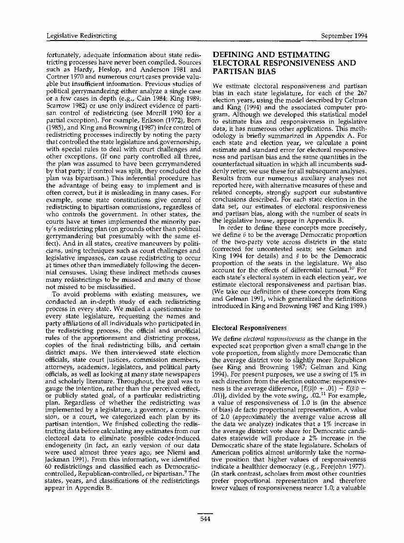
Electoral Responsiveness over Time in Each State, by Region Northeast

1968 1978 1988

year

Midwest

South

1968 1978 1988

year

West

o - partisan redistricting 1988 1978 1988

' - bipartisan redistricting year 1968 1978 1988

year

Source: Calculated from district-level electoral data using JUDGEIT (Gelman and King 1993). For each state, data are included only for years in which all elections were held in single-member districts.

topic for future research would be to work out the conditions under which each normative standard is most appropriate.) Figure 1 presents a descriptive view of electoral responsiveness over time in each state in our data set. Most states have responsiveness values between 1.0 and 3.0. Excevt for the South.

I

responsiveness has gradually dropped over time, just as in the U.S. Congress (King and Gelman, 1991). As the Republicans have gained strength in the South, the legislatures of southern states have become more competitive with increasing electoral responsiveness.

Partisan Bias

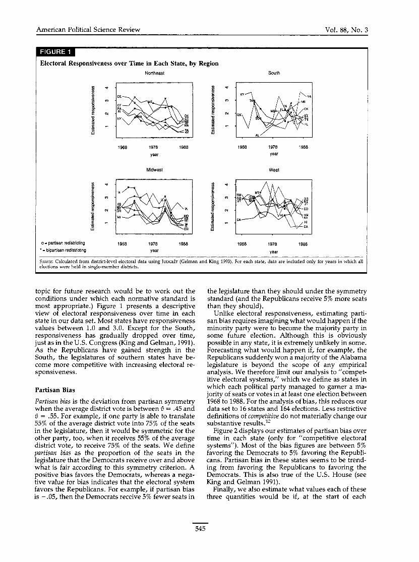
Partisan bias is the deviation from partisan symmetry when the average district vote is between 0 = .45 and fi = -55. For example, if one party is able to translate 55% of the average district vote into 75% of the seats in the legislature, then it would be symmetric for the other party, too, when it receives 55% of the average district vote, to receive 75% of the seats. We define partisan bias as the proportion of the seats in the legislature that the Democrats receive over and above what is fair according to this symmetry criterion. A positive bias favors the Democrats, whereas a negative value for bias indicates that the electoral system favors the Republicans. For example, if partisan bias is - .05, then the Democrats receive 5% fewer seats in

the legislature than they should under the symmetry standard (and the Republicans receive 5% more seats than they should).

Unlike electoral responsiveness, estimating partisan bias requires imagining what would happen if the minority party were to become the majority party in some future election. Although this is obviously possible in any state, it is extremely unlikely in some. Forecasting what would happen if, for example, the Republicans suddenly won a majority of the Alabama legislature is beyond the scope of any empirical analysis. We therefore limit our analysis to "competitive electoral systems," which we define as states in which each political party managed to garner a majority of seats or votes in at least one election between 1968 to 1988. For the analysis of bias, this reduces our data set to 16 states and 164 elections. Less restrictive definitions of competitive do not materially change our substantive result^.'^

Figure 2 displays our estimates of partisan bias over time in each state (only for "competitive electoral systems"). Most of the bias figures are between 5% favoring the Democrats to 5% favoring the Republi- cans. Partisan bias in these states seems to be trend- ing from favoring the Republicans to favoring the Democrats. This is also true of the U.S. House (see King and Gelman 1991).

Finally, we also estimate what values each of these three quantities would be if, at the start of each


Partisan Bias over Time in Each State, by Region Northeast

1968 1978 1988

year

Midwest

South

1968 1978 1988 year

west

'0 V) 2 2 s $ s 0

B E V) 8

o - Democratic redistricting

v - Republican redistricting 1968 1978 1988 1968 1978 1988 - bipartisan redistricting year year

Note: Positive values for estimated partisan bias on the vertical axes in these graphs indicate electoral systems that unfairly favor the Democratic Party; negative values indicate bias in favor of the Republican Party. Calculated from district-level electoral data using JUDGEIT (Gelman and King 1993). For each state, data are included only for years in which all elections were held in single-member districts. Only states with competitive electoral systems are included.

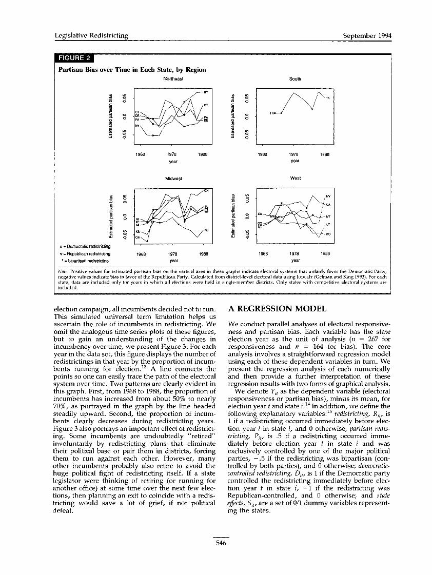
election campaign, all incumbents decided not to run. This simulated universal term limitation helps us ascertain the role of incumbents in redistricting. We omit the analogous time series plots of these figures, but to gain an understanding of the changes in incumbency over time, we present Figure 3. For each year in the data set, this figure displays the number of redistrictings in that year by the proportion of incumbents running for election.13 A line connects the points so one can easily trace the path of the electoral system over time. Two patterns are clearly evident in this graph. First, from 1968 to 1988, the proportion of incumbents has increased from about 50% to nearly 7076, as portrayed in the graph by the line headed steadily upward. Second, the proportion of incumbents clearly decreases during redistricting years. Figure 3 also portrays an important effect of redistricting. Some incumbents are undoubtedly "retired" involuntarily by redistricting plans that eliminate their political base or pair them in districts, forcing them to run against each other. However, many other incumbents probably also retire to avoid the huge political fight of redistricting itself. If a state legislator were thinking of retiring (or running for another office) at some time over the next few elections, then planning an exit to coincide with a redistricting would save a lot of grief, if not political defeat.

A REGRESSION MODEL

We conduct parallel analyses of electoral responsiveness and partisan bias. Each variable has the state election year as the unit of analysis (n = 267 for responsiveness and n = 164 for bias). The core analysis involves a straightforward regression model using each of these dependent variables in turn. We present the regression analysis of each numerically and then provide a further interpretation of these regression results with two forms of graphical analysis.

We denote Yi, as the dependent variable (electoral responsiveness or partisan bias), minus its mean, for election year t and state i.14 In addition, we define the following explanatory variables:15 redistricting, R,, is 1 if a redistricting occurred immediately before election year t in state i, and 0 otherwise; partisan redistricting, Pit, is -5 if a redistricting occurred immediately before election year t in state i and was exclusively controlled by one of the major political parties, -.5 if the redistricting was bipartisan (controlled by both parties), and 0 otherwise; democratic- controlled redistricting, D,, is 1 if the Democratic party controlled the redistricting immediately before election year t in state i, -1 if the redistricting was Republican-controlled, and 0 otherwise; and state effects, Sit, are a set of 011 dummy variables representing the states.

American Political Science Review Vol. 88. No. 3

Proportion of Incumbents Versus Number of Redistrictings, over Time (Averaged over 17 States)

number of redistrictings (out of 17 states)

Regressions for Electoral Responsiveness. We do not use all the explanatory variables for each regression. To assess the effects of redistricting on electoral responsiveness, we estimate the following linear regression:

where pl, P2, p3, and p4 are regression coefficients, y is a vector of regression coefficients, and (Yi,t-lRit) is an interaction term calculated by taking the product of the lagged dependent and redistricting variables.16

Inclusion of the state variables, Sit, is a standard procedure recommended in time series cross-sec- tional literature, where it is called a "fixed effects model" (Hsiao 1986; Stimson 1985). These variables enable us to pool different states safely, guaranteeing that we are comparing (for example) New York in one year with New York in another, rather than New York in one year with Rhode Island in another. (Including all the state variables also makes the constant term in the regression unnecessary.) From a

theoretical perspective, a random effects model might be preferred (e.g., Dempster, Rubin, and Tsutakawa 1981). We repeated all our regressions with random state effects and found no major substantive changes in the results.17

As such, estimating the coefficients in y is important, but the values they take on are not of direct interest; we therefore omit these from our tables. The remaining coefficients are of interest and are interpreted as follows: P1 is the average effect of any redistricting in increasing Y (responsiveness or bias); p2 is generally negative, indicating how much larger the effect of redistricting is for small previous values of Y and how much smaller it is for larger values of Y (p2 is, equivalently, the drop in the persistence in the level of responsiveness between two elections due to a redistricting intervening); P3 is the additional constant effect of partisan versus bipartisan redistricting over and above the average effect; and p, indicates the persistence of Y over time in the absence of redistricting.18

Regressions for Partisan Bias. To estimate the effects of redistricting on partisan bias, we change equation 1 only by substituting Pit with D,. This changes the interpretation of p3 to the constant effect of Demo- cratic- versus Republican-controlled redistricting over and above the average effect. The interpretation of the other coefficients does not change.

It should be possible to improve our model if additional data become available, but in the many alternative models and diagnostic tests we tried, we found no evidence to contradict the model in equation l. We also found the error distribution and autocorrelation structure of the data to be consistent with the time series behavior of the model.19

Although we found no evidence of nonlinearities, the empirical independence of the lagged dependent variable and the redistricting variables makes our specification unreliant upon the linearity assumption in estimating our key causal effects. Finally, the substantive results we are about to present were robust across all reasonable specifications that were consistent with the data.

EVIDENCE

We present our empirical results first for electoral responsiveness and then for partisan bias. We conduct the analyses in each of these sections in analogous fashion and explain our procedures in most detail in the first.


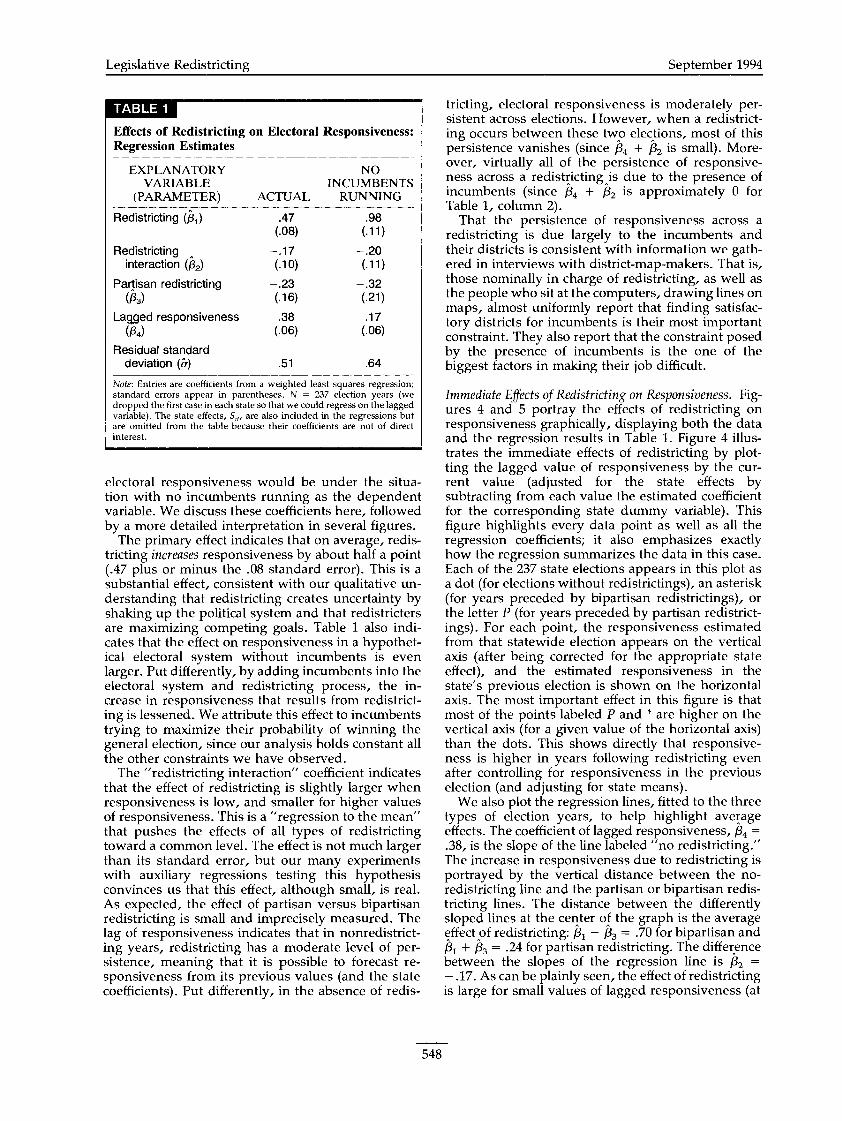
Our regressions explaining electoral responsiveness appear in Table 1. Column 1 reports the estimated regression effects (with standard errors in parentheses) on the actual level of responsiveness. Column 2 reports estimates for a regression with the same explanatory variables but with a forecast of what


Effects of Redistricting on Electoral Responsiveness: Regression Estimates

EXPLANATORY NO VARIABLE INCUMBENTS

(PARAMETER) ACTUAL RUNNING

Redistricting (&) .47 .98 (.08) (.Ill

Redistricting -.I7 - .20 interaction (&) 0) (.Ill

Partisan redistricting - .23 - .32 (83) C16) (.21)

Lagged responsiveness .38 .17 (84) (.06) (.06)

Residual standard deviation (&) .51 .64

Note: Entries are coefficients from a weighted least squares regression; standard errors appear in parentheses. N = 237 election years (we dropped the first case in each state so that we could regress on the lagged variable). The state effects, S,,, are also included in the regressions but are omitted from the table because their coefficients are not of direct interest.

electoral responsiveness would be under the situation with no incumbents running as the dependent variable. We discuss these coefficients here, followed by a more detailed interpretation in several figures.

The primary effect indicates that on average, redistricting increases responsiveness by about half a point (-47 plus or minus the -08 standard error). This is a substantial effect, consistent with our qualitative understanding that redistricting creates uncertainty by shaking up the political system and that redistricters are maximizing competing goals. Table 1 also indicates that the effect on responsiveness in a hypothetical electoral system without incumbents is even larger. Put differently, by adding incumbents into the electoral system and redistricting process, the increase in responsiveness that results from redistricting is lessened. We attribute this effect to incumbents trying to maximize their probability of winning the general election, since our analysis holds constant all the other constraints we have observed.

The "redistricting interaction" coefficient indicates that the effect of redistricting is slightly larger when responsiveness is low, and smaller for higher values of responsiveness. This is a "regression to the mean" that pushes the effects of all types of redistricting toward a common level. The effect is not much larger than its standard error, but our many experiments with auxiliary regressions testing this hypothesis convinces us that this effect, although small, is real. As expected, the effect of partisan versus bipartisan redistricting is small and imprecisely measured. The lag of responsiveness indicates that in nonredistricting years, redistricting has a moderate level of persistence, meaning that it is possible to forecast responsiveness from its previous values (and the state coefficients). Put differently, in the absence of redis-

tricting, electoral responsiveness is moderately per- sistent across elections. However. when a redistricting occurs between these twp elections, most of this persistence vanishes (since p, + P2 is small). More- over, virtually all of the persistence of responsiveness across a redis%ictingnis due to the presence of incumbents (since p4 + P2 is approximately 0 for Table 1, column 2).

That the persistence of responsiveness across a redistricting is due largely to the incumbents and their districts is consistent with information we gath- ered in interviews with district-mav-makers. That is, those nominally in charge of redistricting, as well as the people who sit at the computers, drawing lines on maps, almost uniformly report that finding satisfac- tory districts for incumbents is their most important constraint. They also report that the constraint posed by the presence of incumbents is the one of the biggest factors in making their job difficult.

Immediate Effects of Redistricting on Responsiveness. Fig- ures 4 and 5 portray the effects of redistricting on responsiveness graphically, displaying both the data and the regression results in Table 1. Figure 4 illus- trates the immediate effects of redistricting by plot- ting the lagged value of responsiveness by the current value (adjusted for the state effects by subtracting from each value the estimated coefficient for the corresponding state dummy variable). This figure highlights every data point as well as all the regression coefficients; it also emphasizes exactly how the regression summarizes the data in this case. Each of the 237 state elections appears in this plot as a dot (for elections without redistrictings), an asterisk (for years preceded by bipartisan redistrictings), or the letter P (for years preceded by partisan redistrictings). For each point, the responsiveness estimated from that statewide election avvears on the vertical

L L

axis (after being corrected for the appropriate state effect), and the estimated responsiveness in the state's vrevious election is shown on the horizontal axis. ~ k e most important effect in this figure is that most of the points labeled P and * are higher on the vertical axis (for a given value of the horizontal axis) than the dots. This shows directly that responsiveness is higher in years following redistricting even after controlling for responsiveness in the previous election (and adjusting for state means).

We also plot the regression lines, fitted to the three types of election years, to help highlight avefage effects. The coefficient of lagged responsiveness, P4 = -38, is the slope of the line labeled "no redistricting." The increase in responsiveness due to redistricting is portrayed by the vertical distance between the no- redistricting line and the partisan or bipartisan redistricting lines. The distance between the differently sloped lines at the center of the graph is the average ?ffectpf redistricting: P, - P, = -70 for bipartisan and p, + P3 = -24 for partisan redistricting. The difference between the slopes of the regression line is P2 = - -17. As can be plainly seen, the effect of redistricting is large for small values of lagged responsiveness (at


Effect of Redistricting on Electoral Responsiveness, Next Election

H . . ,P p 5% '9 - .r iij bipartisan redistricting

2 parusan redistricting B,o $ 3 U G - s? 2 m u E 5 .- +-

w" 7 - . . . .

Estimated responsiveness in last election

the left). Or, equivalently, the persistence of responsiveness (as represented by the steepness of the line) is much greater in the absence of redistricting.

Figure 4 helps convey, better than the coefficients in Table 1 can alone, the appropriateness of our regression model for this problem. (For example, one can see the dots on this graph clearly clustered around the no-redistricting line and below the asterisks and Ps.) Perhaps the most important feature of

the graph, confirming that the assumptions of our regression model cannot be rejected by the data, is the absence of any systematic pattern in the data points except those picked up by the regression lines. Finally, Figure 4 shows the unpredictability of redistricting: even after controlling for the lagged responsiveness and state effects, the points on the graph are quite variable. The strong average effects revealed by the regression do not apply to all individual cases.

Effect of Redistricting on Electoral Responsiveness, Next Five Elections JBipanlsan redistricting plan implemented

2 - V)

I c c 9 % X - V) V)

R - $ 2 5 .% 0-0 9 - - g . 2 - iii

4 - 7

Elections after redistricting

Note: The figure shows, for three typical cases, the average effects of a bipartisan plan, relative to what would have happened with no redistricting. Source: Calculated from our JUDGEIT results and the regression in Table 1.


Longer-Term Effects of Redistricting on Responsiveness. Figure 5 displays the average effects on responsiveness (relative to any trend) for the five elections following a redistricting. The horizontal axis indicates the number of elections since redistricting, with the vertical dashed line indicating the implementation of a bipartisan redistricting plan.20 To show the differential effects of redistricting, Figure 5 gives three examples, distinguished by the level of responsiveness in the election before redistricting. All three examples show again that, on average, redistricting sharply increases responsiveness in the first election, with the largest effect occurring for states that had low responsiveness before the redistricting. The effects in the graph are calculated from the regression in Table 1 and the implied AR(1) time series model.

Figure 5 shows that the average redistricting effect is very large in the first year, moderate in the second, much smaller in the third, and nonexistent for the fourth and last years. The effect of redistricting in increasing responsiveness does not last until the fifth election, implying that redistricting is unlikely to contribute to longer-term trends. Hence, the existence of many redistrictings increasing responsiveness is consistent with a secular decline in responsiveness over the two decades in our study (see Figure 1). However, this pattern does not mean that the effect of redistricting on responsiveness is unim- portant. On the contrary, in the typical state, redistricting occurs after every fifth election, and, as a result, its electoral system benefits from higher levels of responsiveness for roughly half of all elections solely because of redistricting. Redistricting thus boosts the responsiveness of a state electoral system significantly higher than it would otherwise be for about half of all elections. Although any single redistricting does not have permanent effects, the decennial redistricting process is a permanent part of every state's electoral system. As a result, redistricting continually and fundamentally alters the character of representative democracy.

Partisan Bias

In addition to its effect on responsiveness, legislative redistricting has an important effect on the relative fortunes of the political parties. Redistricting can affect the proportion of seats that a party controls in the legislature in two ways. The first, which has been the subject of speculation in the literature but only rarely of empirical analyses, is the effect of redistricting on the average district vote. The second is what we call partisan bias-the effect of redistricting on the allocation of seats between the parties given their average district votes. The ultimate effect of redistricting on the division of parties in the legislature is the sum of these two effects. One can use the seat proportion as the dependent variable in a separate regression to estimate this sum directly. Like most researchers, we prefer a separate estimate of the effects on partisan bias so that we can judge the fairness of the electoral system.

Effects of Redistricting on Partisan Bias: Regression Estimates

EXPLANATORY NO VARIABLE INCUMBENTS

(PARAMETER) ACTUAL RUNNING

Redistricting (p,) -.012 - ,012 (.004) (.004)

Redistricting - .63 -.77 interaction (3.J (.16)

Democratic ,010 .003 redistricting (p,) (.005) (.006)

Lagged bias (p,) .77 .55 607) (.09)

Residual standard deviation (&) .014 .015

Note: Entries are coefficients from a weighted least squares regression; standard errors appear in parentheses. The dependent variable is estimated partisan bias; as in Figure 2, where this variable is displayed, positive values indicate state electoral systems which favor the Demo- crats and negative values indicate bias in favor of the Republicans. N = 143 election years (all but the first election in our data set for all states whose electoral systems were "competitive"). The state effects, S,,, are also included in these regressions but are omitted from the table because their coefficients are not of direct interest.

lmmediate Effects of Redistricting on Partisan Bias. We begin by estimating the regression with bias as the dependent variable, conducted in a manner parallel to that for responsiveness. The results appear in Table 2. Many of the key results here are easier to interpret in conjunction with the graphs in Figures 6 and 7. To begin, note that Figure 6 indicates that partisan bias is rarely greater than about 8% (on both axes) in favor of either party. We believe this is because of the numerous constraints on gerrymanderers, as described in the introduction. We turn now to the effects of redistricting on bias by looking first at the baseline of the effect of lagged bias on current bias in the absence of redistricting. This is portrayed in F ig r e 6 as a no-redistricting line with the steep slope of p4 = .77 and indicates that in the absence of redistricting, the level of bias tends to persist much longer than for responsiveness. Because the slope of this line is almost 1, partisan bias changes very little in the absence of redistricting. We therefore expect that whatever effect redistricting has on bias, its effect will take a long time to dissipate.

From this baseline, we can now examine the effects of redistricting. On average, redistricting makes the typical state's electoral system fairer (closer to zero bias) than it would be if redistricting had not occurred. This effect is illustrated in Figure 6 by the asterisks, circles, and triangles (indicating that bipartisan, Democratic, or Republican redistricting, re- spectively, occurred between the two elections), which are generally much closer to 0 on the vertical axis than the dots (election years without redistricting). This means that state electoral systems are closer to no partisan bias following redistrictings.


Effect of Redistricting on Partisan Bias, Next Election (favors Democrats)

Ln

8 V) m " p

Demouatic redistricting 5 # bipartisan redistricting E-" " Republican redistricting

= 3 s m .= .; 3 LU

(favors Republicans) I I I

Estimated partisan bias in last election

This effect is summarized by the three redistricting lines being much flatter (and closer to 0 on the vertical axis for most of the range of the horizontal axis) than the no-redistricting line. (The difference in the slopes of the redistricting and no-redistricting lines is the redistricting interaction coefficient, p2 = - .63.)

Thus, no matter how fair or biased the electoral system is to begin with, the typical redistricting plan, whether Democratic, Republican, or bipartisan-controlled, will produce a fairer electoral system.'' This

result is consistent with evidence from individual cases in which the largest effects of redistricting change an existing huge bias in favor of one party to small bias in favor of the other.22

The reason that any redistricting reduces bias appears to be the role that redistricting has in shaking up the political system in combination with the many constraints on the mapmakers. Shaking up a system that is effectively constrained to have partisan bias between about -c8% of fairness cannot have an enor-

Elections after redistricting

Effect of Redistricting on Partisan Bias, Next Five Elections IDemocratic-mntmlled redistricting plan implemented

Note: The figure shows, for three typical cses, the average effects of a Democratic plan, relative to what would have happened with no redistricting. Source: Calculated from our JUDGEIT results and the regression in Table 2.

(favors Democrats)

t

- 2 - s

2 #

-

\ 3 L

- t

(favors Republicans)


mous effect (although much smaller effects will be quite significant to individual incumbents and political parties). Moreover, if there is already a high level of bias, due to the previous decade's redistricting (or, more likely, to demographic and mobility changes in the population over the decade), any political turmoil will have a higher probability of moving the system toward fairness since there is simply more room to move in that direction.

This powerful role redistricting has in producing fairer electoral systems does not imply that Demo- cratic redistrictings produce the same result as Re- publican or bipartisan ones. To the contrary, the order of ths three redistricting lines in Figure 6 (and the effect p3 in Table 2) indicates that Democratic- controlled redistricting plans typically bias the electoral system toward the Democrats by about 1% (with a standard error of .5%) more than a bipartisan plan. Republican-controlled plans favor the Republicans by about the same amount. Thus, the difference between a Democratic- and Republican-controlled redistricting plan is, on average, an increase in partisan bias of about 2% for the party in control (and a corresponding decrease of about 2% for the other party).23 The variability of individual results in Figure 6 also indicates that redistricting can have somewhat more or less powerful effects than the average results summarized by the regression lines. With fewer data, less efficient statistical methods, or less careful cate- gorization of redistrictings by partisan control, we may not have been able to distinguish the systematic partisan effects of redistricting from the inherent variability in the system (as seemed to be the case with some existing research).

Finally, Table 2, column 2, displays the effects of redistricting on partisan bias in the hypothetical situation where no incumbents run for reelection. The partisan effect of redistricting, P3, is statistically (and substantively) indistinguishable from zero in this case. Since incumbents are key actors in either drawing the lines or influencing the line-drawers, this result is fully consistent with the substance of redistricting that we portrayed in the introduction. Incum- bents lead the troops into most redistricting battles. That they and their vote-getting abilities would be considered as givens when drawing the district lines is just what we would expect. If, as in our counterfactual condition, many incumbents were unexpect- edly defeated, the redistricting might turn out to have very different political consequences.

Thus, partisan-controlled redistricting plans produce electoral systems that favor the party in control more than the opposition party. However, the range of possible outcomes that any redistricter is able to produce, given the complicated constraints and uncertainties, is usually in the neighborhood of near- zero bias. The differences within this neighborhood are still highly significant to the partisans (as we shall further demonstrate), but the overall existence of redistricting constrains bias to within this small and comparatively fair range.

Longer-Term Effects of Redistricting o n Partisan Bias. We examine the effects of redistricting on partisan bias over the next five elections with Figure 7, which is based on the regression (and the implied autoregres- sive time series model with interventions) in Table 2, column 1. This figure is directly analogous to Figure 5, except that the only intervention represented here is a Democratic-controlled redistricting plan. (Esti- mates for the effects of a Republican-controlled plan are a mirror image of these.) As can be seen clearly by the three lines converging from election year 0 to election year 1, large Republican and even Demo- cratic biases are substantially reduced because of this redistricting. However, the Democrats still produce an electoral system biased in their favor, since all three lines are above zero. Finally, we can see that this immediate effect persists in large measure over the remaining election years before the next redistricting.

Effect of Redistricting on the Average District Vote

We studied the effect of redistricting on votes with the same regression model we developed for bias but using d in place of bias as the outcome variable and also including dummy variables for each election year, to control for national swings in the vote. The results indicate that partisan redistrictings increase the proportion of votes for the candidates of the controlling party by an average of about 1% (plus or minus a standard error of .5%) as compared to a bipartisan redistricting. Because responsiveness averaged over all states and elections in our data is about 2.0, this effect on votes typically increases the seat proportion for the party controlling the redistricting by about 2% (the 1 % effect on votes multiplied by the typical responsiveness of 2.0) as compared to bipartisan control. Thus, the difference in seats between a Democratic- and Republican-controlled redistricting plan is, on average, a substantial 4% of seats. The causal mechanism by which this effect works is probably as follows. A partisan redistricting produces additional districts that the party in control of redistricting is likely to win, as we have demonstrated. As a result, this party finds it easier to field better candidates, which, in turn, produces more votes for those candidates (see Cain 1985; Canon, Schousen, and Sellers 1993).'~

Unlike the other regression models estimated herein, the regression for votes relies very heavily on the assumption of linearity in order to establish the causal effect of redistricting. The reason is that only in the model for votes are the key causal effects (the redistricting variables) highly correlated with one of the control variables (lagged votes). That is, states with higher Democratic vote proportions in the election before redistricting are more likely to have Dem- ocratic-controlled redistricting plans implemented. The correlation with the lagged variable is much weaker in the regressions for bias and responsiveness. The dependence on the linearity assumption of our inference for the effect of redistricting on votes is


well within the standards followed throughout the social sciences where key causal variables are often highly correlated with important control variables. As such, we are confident of these estimates. However, we do not proceed with more detailed analyses of this effect (including such features as its persistence over time, as we did for responsiveness), since they would not be as certain as all other results herein, where we are in the fortunate situation of having causal infer- ences that meet even higher standards (and thus greater certainty) than usual.

Total Effect of Redistricting

Finallv, we can add the effect of redistricting on , , " partisan bias (seats given a fixed average district vote) to the effect of redistricting on the division of votes between the parties. This sum gives the total effect of redistricting on the division of seats in the legislature between the parties: if one party controls a redistricting plan, it can expect, on average, to receive approximately 6% of the seats that the other party would have won if it controlled the redistricting. That is, the party drawing the district lines receives, on average, about 6% more seats-and the opposition party 6% fewer seats-than if the opposition party had controlled the mapmaking. Thus, even though redistricting makes the electoral system substantially fairer overall than if there were no redistricting, the difference between Democratic and Republican control over the drawing of district maps is still one that politicians are rightfully concerned about.

We also estimated the effect of redistricting on seats directly, by regressing seats S on redistricting type, controlling for state effects, lag seats, the lag-redistricting interaction (as usual), and election year effects. The results of this regression-an effect of 3.2% for the party controlling redistricting, with a standard error of 1.3%-are consistent with our separate analysis of votes and bias. (An effect of 3.2% for partisan redistricting corresponds to 6.4% when comparing Democratic to Republican plans.) In general, we prefer to analyze votes and bias separately, because each is an important consequence of the partisan effect of redistrictingz5 We see the direct regression of seats as a confiimation of our more important results.

CONCLUDING REMARKS ON THE BENEFITS OF REDISTRICTING

As described, our empirical results are consistent with the conflictual and uncertain process of legislative redistricting and the competing goals of redistricters. They also help resolve two important controversies in American politics over the consequences of legislative redistricting for partisan bias and electoral responsiveness. For one, our results demonstrate that contrary to all previous researchers, redistricting in state legislatures has substantially increased elec-

toral responsiveness and kept it higher than it would be otherwise for about half of all elections in each state. The effects of any one redistricting are not permanent, but the decennial redistricting process repeatedly injects the political system with a healthy dose of increased responsiveness. For partisan bias, we have identified a difference in the causal question asked by two groups of researchers, making both sides in this controversy correct to a degree. Our results indicate that partisan and bipartisan redistricting plans reduce bias overall, leading to fairer electoral systems than if there had been no redistricting, but the difference between Democratic-, bipartisan-, and Republican-controlled redistricting plans within this smaller and comparatively fairer region are still politically significant.

We now briefly organize these results from two perspectives. First, individual legislators involved in redistricting can be seen as simultaneously attempting to maximize three partly inconsistent goals: they try to increase the probability of winning or avoiding a primary, winning the general election (conditional on winning the primary), and helping their party win a majority of seats in the legislature. Those responsi- ble for drawing the district lines, whether partisan or bipartisan, always operate in a highly constrained and uncertain environment. The final redistricting plan is usually the result of the process of achieving consensus among incumbents and others, subject to the formal and informal constraints; this process usually produces a plan that weights party advantage heavily.

When incumbents give up votes in order to increase the probability of being in the majority party, responsiveness increases. It also increases when other incumbents retire to avoid the political fight altogether and due merely to changes in district lines and to wholesale increases in uncertainty. Giving up votes in this way also means that Democratic-controlled redistricting plans usually favor the Demo- crats more than those controlled by the Republicans. However, in order to retain their seats, they do not go too far in trying to achieve this goal. Hence, partisan bias does not favor their party as much as it could. These constraints on partisan bias during redistricting are much more substantial than during the rest of the decade, when changes in demographics, turnout, and the configuration of candidates can cause comparatively larger changes in bias and responsiveness.

A second way to organize these results is to review what they say about the benefits and costs of redistricting for states' representative democracies. The purpose of reapportionment and redistricting is to guarantee that the number of citizens in each district if roughly the same, at least at the start of each decade. Redistricting obviously accomplishes this minimal goal. However, as most political scientists recognize, population equality guarantees almost no form of fairness beyond the numerical equality of population. Even aside from issues raised by count- ing citizens (rather than voting-age Americans or voters), by representing ethnic minorities fairly, or


attempting to ensure that each citizen has an equal say in the policy outcome (which may be impossible to achieve, given such internal legislative rules as seniority on committees), there are the questions of what redistricting does intentionally or unintention- ally to the features of our representative democracy that we have discussed here. Allowing state legislators to redistrict opens up the possibility of partisan gerrymanders, incumbent protection plans, and other apparently insidious consequences of the simple task of drawing district lines around equal-sized groups of Americans.

The vast majority of American political scientists have adopted the normative position that healthy representative democracies have low levels of partisan bias and high levels of electoral responsiveness. Our empirical results should make those who support this dominant position yearn for the next redistricting period. The political turmoil created by legislative redistricting creates political renewal. Many of the goals sought by proponents of term limitations are solved by legislative redistricting. Even the repu- tation of the "egregious" partisan gerrymander has been somewhat rehabilitated: not only does redistricting perform the simple task of getting the num- bers right, but redistricting has tended to reduce partisan bias and increase electoral responsiveness.

It is true that bipartisan redistricting produces as high levels of responsiveness and lower levels of partisan bias than partisan-controlled redistricting plans. Moreover, Democratic- and Republican-controlled plans have very different consequences for the parties. One can also still find specific examples of substantial partisan gerrymanders that produce much more partisan bias. These results provide good reason to support a proposal to require bipartisan control of all redistricting processes. If a legislature is incapable of forging a bipartisan agreement, then alternating, or randomly assigned, control of redistricting would also accomplish many of the same benefits. Our results demonstrate that earlier objec- tions to this proposal based on the belief that it will usually create incumbent protection plans (and hence unresponsive electoral systems) are unfounded.

Finally, our results bear directly on the role the courts might choose in resolving partisan gerrymandering claims. The U.S. Supreme Court declared partisan gerrymandering to be justiciable in Davis v. Bandemer (1986), but it has not yet made clear whether the standards of fairness will be set so that a plaintiff would have a chance of meeting them. On the basis of its recent decisions (e.g., Voinovich v. Quilter 1993), it seems clear that the Supreme Court would probably prefer not to be involved in partisan redistricting matters, and our results provide them with a clear public policy ju~tification.'~ Individual state redistricting plans sometimes do produce very unfair electoral systems, but on average, recent state redistricting~, even when unattended by the courts, have reduced partisan bias and increased responsiveness. Far from being a scourge on the political system in

need of major reforms, legislative redistricting has invigorated American representative democracy.

APPENDIX A: ESTIMATING RESPONSIVENESS AND BIAS

We used the method of Gelman and King (1994), implemented in our computer program called JUDGEIT (Gelman and King 1993), to estimate the electoral responsiveness and partisan bias from individual district-level data in each state legislative election. The results of these estimations are displayed in Figures 1 and 2. (JUDGEIT and the statistical model underlying our method are described in detail in Gelman and King 1994.) Our method is a straightforward and substantially improved version of our previous method (see Gelman and King 1990; King and Gelman 1991) for defining, estimating, predicting, or evaluating under counterfactual conditions concepts such as seats-votes curves, partisan bias, electoral responsiveness, the expected or predicted vote in each district in a legislature, the probability that a given party will win the seat in each district, the proportion of incumbents or others who will lose their seats, the proportion of women or minority candidates to be elected, the incumbency advantage and other causal effects, the likely effects on the electoral system and district votes of proposed electoral reforms (e.g., term limitations, campaign spend- ing limits, and drawing majority-minority districts), and any other properties of an electoral system that can be defined in terms of vote shares in districts. The method is based on a statistical model that can be applied to virtually any legislature with two major parties and plurality rule elections in districts.

Here we shall briefly outline how our model is applied to estimating responsiveness and partisan bias. As described, we define these quantities based on the seats-votes curve, which in turn we define as the expected proportion of seats, given the average district vote. (These definitions were first given in Gelman and King 1990 and King and Gelman 1991 and are based on King and Browning 1987 and King 1989.) A large literature on the seats-votes curve has accumulated over the past half-century, and several methods have been applied to estimate the function of seats, given votes (or, more precisely, expected seats, given votes). One approach, which uses minimal modeling assumptions, is to estimate the seats- votes curve by a regression of aggregate results from several election years; see, e.g., Tufte 1973). This approach suffers from inefficiency (using aggregate, not district-level, vote information) and, more impor- tantly, cannot be used to measure year-to-year changes, such as we are interested in here. The other traditional approach to estimating the seats-votes curve has been based on the model of "uniform partisan swing" (see, e.g., Butler 1951), a determin- istic model that, without modification, applies to no known electoral system.


Our method can be seen as a generalization of uniform partisan swing, with two major improvements. First, we model variability in district election outcomes beyond a uniform statewide swing, thus making the model far more realistic. Second, we include explanatory variables to improve predictions, thus harnessing the full power of regression modeling for district-level data. We also verified each of these assumptions in extensive analyses of all available data on state legislative and congressional elections. We here use past election results, uncontested status, the party of the winner in the previous election, and incumbency as explanatory variables. In addition, we treat uncontested elections in a special way (see Gelman and King 1994).

Although our model applies to any electoral system with two parties or groups of parties, we use the labels "Democratic" and "Republican" to fix ideas more clearly. We assume a legislature comprising n single-member districts and denote v i as the Demo- cratic proportion of the two-party vote in each district i and v as the set of votes for all districts (v,, v,, . . . , v,). The votes v will be predicted by k explanatory variables, which can together be written as n x k matrix, X. We model the district vote outcomes with a random components linear regression of v on X, v = Xp + y + E, where p is a vector of k parameters that we estimate from each state election, and y and E are two vectors of independent error terms. The variable E is a traditional random error term; y is the "random component" error term, which helps correct for the fact that the X variables do not completely describe the state of the electoral system at the start of the

campaign due to the omission of relevant variables and measurement error in the variables included. For each district i, the error terms are assigned independent normal distributions, yi - N(0, a;), ei - N(0, a:), with variances a; and a: that we estimate from several years of election data for each state.

The parameters of this model to be estimated-4, 4, and @--are not usually of primary interest in evaluating electoral systems and redistricting plans (although p is in some cases of interest in evaluating causal effects). Instead, we define theoretically all the quantities of interest, including the seats-votes curve, responsiveness, and partisan bias, and then compute posterior distributions of all these quantities using Bayesian simulation. The estimates and standard errors of responsiveness and partisan bias used in this study are just the posterior mean and standard deviation of these quantities, estimated separately for each state election.

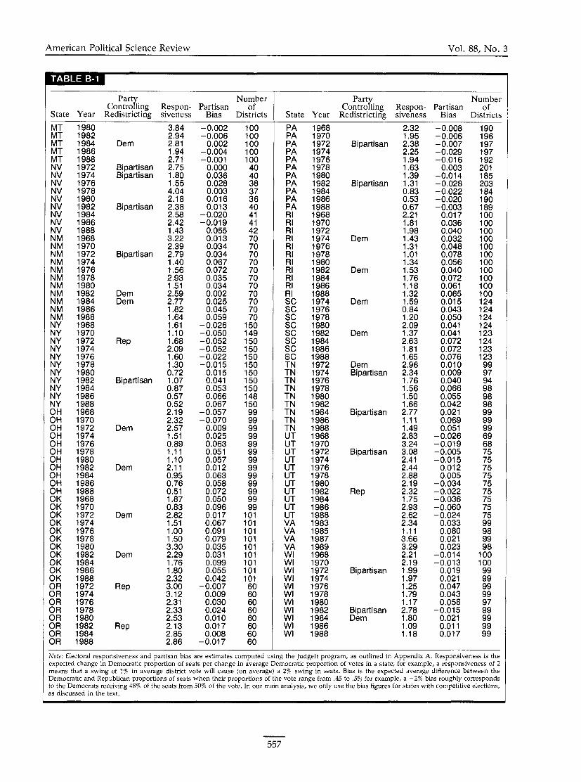
APPENDIX B: ESTIMATES OF BIAS AND RESPONSIVENESS FOR STATE ELECTIONS

The posterior mean estimates, along with redistricting information, are presented in Table B-1. Posterior standard deviations, as well as the district-level data upon which the estimates were based, are available from the Inter-University Consortium for Political and Social Research in a Class V data set under the authors' names, or from the authors.


Estimates of Bias and Responsiveness and Redistricting Information for State Elections

Party Number Controlling Respon- Partisan of

State Year Redistricting siveness Bias Districts

Dern

Bipartisan

Dern

Rep

Rep

Rep

Dern

Rep

Bipartisan

Dern

Bipartisan

Dern

Rep Rep

Party Number Controlling Respon- Partisan of


Rep.

Bipartisan Bipartisan

Bipartisan

Dern

Dem

Bipartisan

Bipartisan

Dern

Dem

Dem

Rep

Dern Dern

Bipartisan

Bipartisan

Dern


Number Respon- Partisan of siveness Bias Districts

Dern

Bipartisan Bipartisan

Bipartisan

Bipartisan

Dern Dern

Rep

Bipartisan

Dern

Dern

Dern

Dern

Rep

Rep

Number Contro ling Respon- Partisan of


Bipartisan

Bipartisan

Dern

Dern

Dern

Dern

Dern Bipartisan

Bipartisan

Bipartisan

Rep

Bipartisan

Bipartisan Dern

L

Vote: Electoral responsiveness and partisan bias are estimates computed using the JudgeIt program, as outlined in Appendix A. Responsiveness is the 2xpected change in Democratic proportion of seats per change in average Democratic proportion of votes in a state; for example, a responsiveness of 2 neans that a swing of 1% in average district vote will cause (on average) a 2% swing in seats. Bias is the expected average difference between the Iemocratic and Republican proportions of seats when their proportions of the vote range from .45 to .55; for example, a -2% bias roughly corresponds o the Democrats receiving 48% of the seats from 50% of the vote. In our main analysis, we only use the bias figures for states with competitive elections, IS discussed in the text.


Notes

We thank Ken Benoit and Mike Ting for research assistance; Jim Alt, Bruce Cain, Normal Luttbeg, and Michael McDonald for helpful comments; and the National Science Foundation for research grant SBR-9223637. Gary King also thanks Nuff- ield College, Oxford University, for a visiting fellowship; the John Simon Guggenheim Memorial Foundation for a fellowship; and the National Science Foundation for research grant SBR-9321212. All data and information necessary to replicate the results in this article are available from the Inter-Univer- sity Consortium for Political and Social Research in a Class V data set listed under our names. The computer program we used for this work is called JudgeIt and is available from the authors, the ICSPR, or on the Internet via "gopher" or "anonymous FTP" from haave1mo.harvard.edu.

1. We learned of this story from telephone interviews with justices, politicians, and civil servants in Michigan, while collecting our data.

2. In private conversations with us, members of Congress often volunteer their strong support for increasing the size of Congress so that no state would lose a member at redistricting time. However, they also believe that such a proposal would not stand a chance of passing because it seems so self-serving.

3. For example, we observed several white Democratic legislators in one state succeed in drawing many black voters out of their districts. Because blacks vote overwhelming for the Democrats, this action reduced these legislators' likely general election vote margins, if they got to the general election. However, since voters often prefer to be represented by others from their ethnic group, these new district lines may have increased these white legislators' probabilities of winning or avoiding a primary election.

4. During the redistricting process in one state, we spoke to an incumbent whose new district would have probably given him about 75% of the vote, almost exactly what he had before the redistricting. Yet he went to great extents to oppose the new plan because the opposition party, which controlled the redistricting, had, as he said, "ruined his life." It previously took him under an hour to drive to anywhere in his district, but the new district would be stretched almost all the way across the state. In addition, all four of his district offices and even his childrens' schools were drawn out of the district.

5. Even trying to improve their party's chance of winning a majority of seats is in the narrow self-interest of incumbent legislators, since majority party members in most states have more staff, are chairs of committees, gain additional visibility, and are better able to accomplish their policy goals and satisfy their constituents. As one legislator explained it to us, being in the majority party is also "a lot more fun."

6. We have applied the methods described herein to other measures of electoral competitiveness and found only trivial substantive differences from the results reported in the text using our responsiveness measure.

7. We have checked a sample of these ICPSR data with our own data coded directly from the blue books published by several state governments. We found a few errors (and reported them to the ICPSR), but overall these data are remarkably clean and far more reliable than, for example, the ICPSR collections of U.S. House and Senate data.

8. We do not distinguish between bipartisan and nonpar- tisan redistricting plans. In most states, it is difficult or impossible to do so. Some previous analyses also used a separate category for court-imposed plans, but many courts (especially state courts) are widely known to be very partisan.

9. Errors in this variable, if any, are almost certainly unre- lated to other variables in our analysis.

10. We studied the effects of differential turnout across districts on our estimates by repeating all analyses after substituting the statewide vote for the two parties (i.e., the total votes for the Democratic candidates cast statewide as a proportion of major party votes) in place of the average district vote, fi. (For a discussion of the role of turnout in these two definitions of statewide vote, see Ansolabehere, Brady,

and Fiorina 1988.) Although the levels and patterns of responsiveness and bias did change in some states, the effects of redistricting on these quantities were not materially different from those based on fi. That is, in the ensuing analyses, Figures 1 and 2 changed in some ways, but Figures 4-7 (and Tables 1 and 2) changed in only substantively trivial ways.

11. Using average electoral responsiveness measured at fi between .45 and .55 (see Gelman and King 1994) gives very similar results when applied to the present analysis.

12. We also analyzed responsiveness for these subsets of data and found no relevant changes.

13. To maintain comparability, each point on the figure is averaged over only those 17 states that are in our data set for all 20 years.

14. Subtracting the mean from the dependent variable does not affect any substantive results, but it allows the coefficients of redistricting to be interpreted as effects for the average case.

15. The specific codes we use to represent the dummy variables make interpretation convenient but are not otherwise required or consequential.

16. To improve the estimation, we use weighted least squares with the estimated standard error of each observation (our estimated value for responsiveness), pooled within each state, to compute the weight. This is a standard procedure in general and in this literature (see King 1991; King and Browning 1987).

17. The random-effects model altered the regression results in three ways: (1) most of the standard errors decreased slightly, (2) the estimated state effects decreased, and (3) the estimated coefficients of the lagged variables increased. All these changes could be considered as improvements in the model fit, and all are consistent with the theory of random- effects models. However, we used the simpler linear regression model, because the estimated causal effects of interest did not change materially.

18. Another way to interpret equation 1 is by noting that the effect of R,, (redistricting) on Y,, (responsiveness or bias) is (PI + /3zY,,t-l), or, equivalently, the effect of Y,,,_, (last election's responsiveness or bias) on Yit is (p, + pzR,,).

19. Equation 1 is a form of an AR(1) time series model. Conditional on the first lag, which is estimated, the model implies a geometric decline in the coefficients for subsequent lags. To evaluate this assumption, we estimated separate regressions with lags 1, 2, 3, and 4 of redistricting, omitting cases with intervening redistrictings. In all cases, we could not reject the assumption that the correlations followed the AR(1) pattern. For example, the theoretical and estimated lag coefficients for responsiveness are as follows:

Lags Theoretical Estimated (s.e.)

They decline as expected, consistent with the theoretical values based on the lag 1 coefficient of .40. (Note that the estimated coefficients at lags 3 and 4 are smaller than their standard errors.) Analysis of partisan bias gave similar results.

20. In the vast majority of states five elections, at most, are held under any redistricting plan. Since the estimated difference between the effects of bipartisan and partisan plans on responsiveness is small, we omit an analogous figures for partisan plans; it looks very similar to Figure 5.

21. Another way to look at this is with descriptive statistics: the average absolute value of bias in years following redistricting was .016, compared to an average absolute value of ,028 in nonredistricting years.

22. The biggest example of this-indeed, the largest effect of redistricting ever noted in the academic literature to our knowledge-is the Ohio State Legislature in 1972. See Figure 2 and the more detailed analyses in Gelman and King 1990.

23. We find no evidence of a difference between the aver-


age absolute size of an effect created by Democratic and Republican mapmakers.

24. We find little evidence that redistricting plans typically have an effect by selective placement of nonvoters.

25. In addition, as noted, the causal inference for bias is especially reliable because lagged bias, unlike lagged seats and votes, does not correlate strongly with the type of redistricting.

26. The Supreme Court wrote in Voinovich v. Quilter (1993):

Time and again we have emphasized that "reapportionment is primarily the duty and responsibility of the State through its legislature or other body, rather than of a federal court." Growe v. Emison, 507 U.S. (1993), supra, (quoting Chapman v. Meier, 420 U.S. 1, 27 [1975]). Accord, Connor v. Finch, 431 U.S. 407,414 (1977) ("We have repeatedly emphasized that 'legislative reapportionment is primarily a matter for legislative consideration and determina- tion' " [quoting Reynolds v. Sims, 377 U.S. 533, 586 (196411.)

References

Abramowitz, Alan. 1984. "Partisan Redistricting and the 1982 Congressional Elections." Journal of Politics 45:767-70.

Ansolabehere, Stephen, David Brady, and Morris Fiorina. 1988. "Turnout and the Calculation of Swing Ratios." Research Paper No. 990. Stanford University Graduate School of Business.

Born, Richard. 1985. "Partisan Intentions and Election Day Realities in the Congressional Redistricting Process." Amer- ican Political Science Review 79:305-19.

Bullock, Charles. 1975. "Redistricting and Congressional Sta- bility, 19621972." Journal of Politics 37:569-75.

Burnham, Walter Dean. 1974. "Communication." American Political Science Review 68:207-13.

Butler, David E. 1951. Appendix to The British General Election of 1950. Ed. H . G. Nichols. London: Macmillan.

Cain, Bruce. 1984. The Reapportionment Puzzle. Berkeley: Uni- versity of California Press.

Cain, Bruce. 1985. "Assessing the Partisan Effects of Redis- tricting." American Political Science Review 79:320-33.

Campagna, Janet, and Bernard Grofman. 1990. "Party Con- trol and Partisan Bias in 1980s Congressional Redistricting." Journal of Politics 52:124258.

Canon, David, Matthew Schousen, and Patrick Sellers. 1993. "The Supply Side of Congressional Redistricting: Race and Strategic Politicians, 1972-1992." Presented at the annual meeting of the Midwest Political Science Association, Chi- cago.

Cortner, Richard C. 1970. The Apportionment Cases. New York: Norton.

Cranor, John D., Gary L. Crawley, and Raymond H. Sheele. 1989. "The Anatomy of a Gerrymander." American Journal of Political Science 33:222-39.

Davis v. Bandemer 1986. 106 S.Ct. 2797. Dempster, A. P., D. B. Rubin, and R. K. Tsutakawa. 1981.

"Estimation in Covariance Components Models." Journal of the American Statistical Association 76:341-53.

Dixon, Robert G., Jr. 1968. Democratic Representation. New York: Oxford University Press.

Erikson, Robert S. 1972. "Malapportionment, Gerrymander- ing, and Party Fortunes in Congressional Elections." Amer- ican Political Science Review 66:1234-45.

Ferejohn, John A. 1977. "On the Decline of Competition in Congressional Elections." American Political Science Review 71:166-76.

Gelman, Andrew, and Gary King. 1990. "Estimating the Electoral Consequences of Legislative Redistricting." Jour- nal of the American Statistical Association 85:274-82.

Gelman, Andrew, and Gary King. 1993. "JUDGEIT: A Program for Evaluating Electoral Systems and Redistricting Plans." Technical report and computer program. Harvard University.

Gelman, Andrew, and Gary King. 1994. "A Unified Method of Evaluating Electoral Systems and Redistricting Plans." American Journal of Political Science 38:514-554.

Glazer, Amihai, Bernard Grofman, and Marc Robbins. 1987. "Partisan and Incumbency Effects in the 1970s Congres- sional Redistricting." American Journal of Political Science 30:680-701.

Gopoian, J. David, and Darrell M. West. 1984. "Trading Security for Seats: Strategic Considerations in the Redis- tricting Process." Journal of Politics 46:1080-96.

Green, Paul M. 1982. "Legislative Redistricting in Illinois 1871-1982: A Study of Geo-Political Survival." In Redistrict- ing: A n Exercise in Prophecy, ed. Anna J. Merritt. Chicago: University of Illinois Institute of Government and Public Affairs.

Hacker, Andrew. 1963. Congressional Districting: The lssue of Equal Representation. Washington: Brookings.

Hardy, Leroy, Alan Heslop, and Stuart Anderson, eds. 1981. Reapportionment Politics: The History of Redistricting in the Fifty States. Beverly Hills: Sage.

Hsiao, Cheng. 1986. The Analysis of Panel Data. New York: Cambridge University Press.

Kendall, M. G., and A. Stuart. 1950. "The Law of the Cubic Proportion in Election Results." British Journal of Sociology 1:193-96.

King, Gary. 1989. "Representation through Legislative Redis- tricting: A Stochastic Model," American Journal of Political Science 33:787-824.

King, Gary. 1991. "Constituency Service and Incumbency Advantage." British Journal of Political Science 21:119-28.

King, Gary, and Robert Browning. 1987. "Democratic Repre- sentation and Partisan Bias in Congressional Elections." American Political Science Review 81:1251-76.

King, Gary, and Andrew Gelman. 1991. "Systemic Conse- quences of Incumbency Advantage in the U.S. House." American Journal of Political Science 35:llO-38.

Mayhew, David R. 1971. "Congressional Representation: Theory and Practice in Drawing the Districts." In Reappor- tionment in the 1970s, ed. Nelson W. Polsby. Berkeley: University of California Press.

Morrill, Richard. 1990. "A Geographer's Perspective." In Political Gerrymandering and the Courts, ed. Bernard Grof- man. New York: Agathon.

Niemi, Richard, and Simon Jackman. 1991. "Bias and Respon- siveness in State Legislative Districting." Legislative Studies Quarterly 16:183-202.

Niemi, Richard, and Laura R. Winsky. 1992. "The Persistence of Partisan Redistricting Effects in Congressional Elections, in the 1970s and 1980s." Journal of Politics 54:565-72.

Owen, Guillenno, and Bernard Grofman. 1988. "Optimal Par- tisan Gerrymandering." Political Geography Quarterly 7:5-22.

Scarrow, Howard. 1982. "Partisan Gerrymandering-hvidi- ous or Benevolent? Gaffney v. Cummings and Its Aftermath." Journal of Politics 442310-21.

Stirnson, James. 1985. "Regression in Space and Time: A Statis- tical Essay." American Journal of Political Science 29:914-47.

Tufte, Edward. 1973. "The Relationship between Seats and Votes in Two-Party Systems." American Political Science Review 67:540-54.

Voinovich v. Quilter. 1993. 113 S.Ct. 1149.

Andrew Gelman is Assistant Professor of Statistics, University of California- Berkeley, Berkeley, CA 94720. E-mail: [email protected]

Gary King is Professor of Government and Director, Harvard Data Center, Harvard University, Cambridge, MA 02138. E-mail: [email protected]

Enhancing democracy through legislative redistricting

Documents

Enhancing democracy through legislative redistricting