Chapter 10 Sinusoidal Steady- State Power Calculations

In Chapter 9 , we calculated the steady state voltages and currents in electric circuits driven by sinusoidal sources

We used phasor method to find the steady state voltages and currents

In this chapter, we consider power in such circuits

The techniques we develop are useful for analyzing many of the electric devices we encounter daily, because sinusoidal sources are predominate means of providing electric power in our homes, school and businesses

Examples Electric Heater which transform electric energy to thermal energy

Electric Stove and oven Toasters Iron Electric water heater And many others

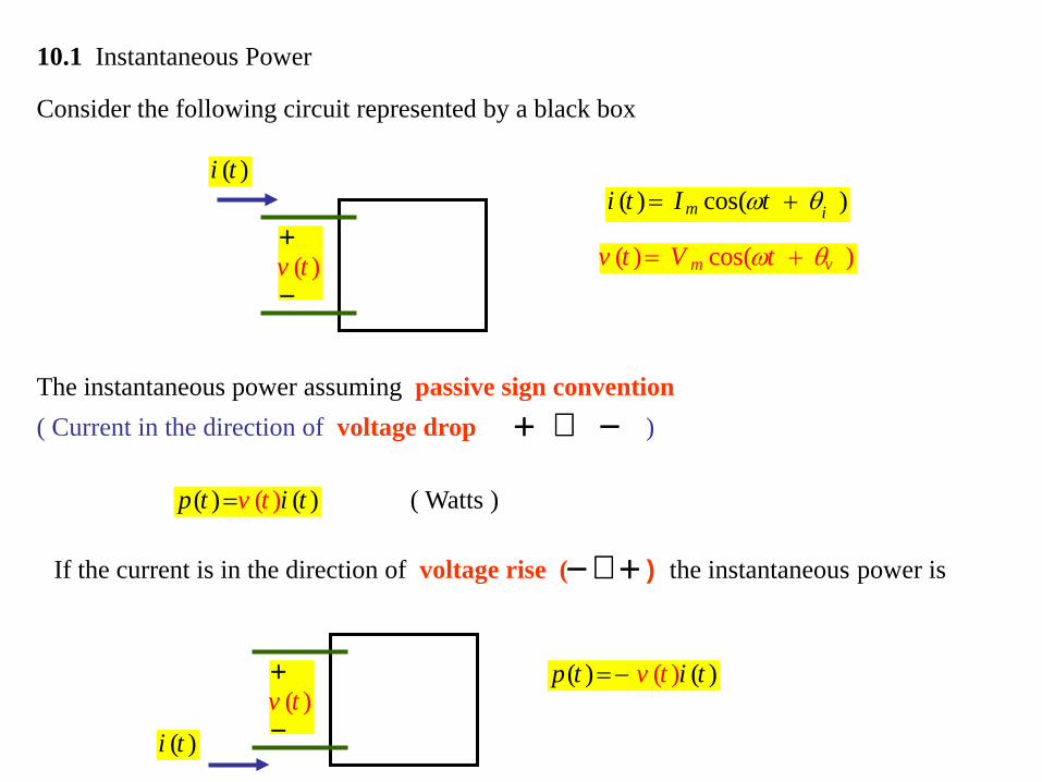
10.1 Instantaneous Power

Consider the following circuit represented by a black box

( )i t

( )v t+

−

( ) cos( )m ii t I tω θ= +

( ) cos( )vmv t V tω θ= +

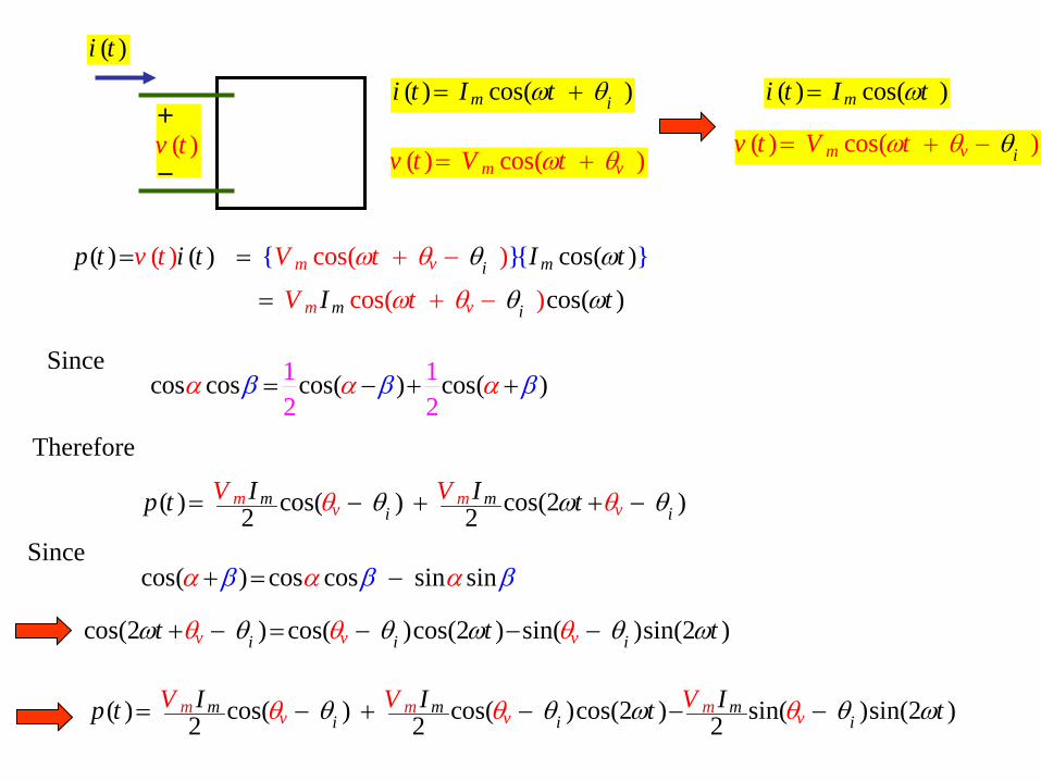
The instantaneous power assuming passive sign convention ( Current in the direction of voltage drop + − )

(( ) ( ))v tp t i t= ( Watts )

If the current is in the direction of voltage rise (− + ) the instantaneous power is

(( ) ( )) vp tt i t= −

( )i t( )v t

+

−

( )i t

( )v t+

−

( ) cos( )m ii t I tω θ= +

( ) cos( )vmv t V tω θ= +

(( ) ( ))v tp t i t= cos( ) cos ( )mivmV t I tω θθ ω+= −

cos( cos( ) )m vm iI tV tω θ θ ω−= +

1 12

cos cos cos( ) cos2

( )α αβ β βα= − + +Since

Therefore

( ) cos( )mi t I tω=

( ) cos( )v imv t V tω θ θ= + −

cos( ) cos cos sin in sα αβ β α β+ = −Since

cos(2 ) cos( )cos(2 ) sin( )sin(2 )v vi i ivt t tω θ θ ω θθ θ ωθ+ − = − − −

( ) cos( ) cos( )cos(2 ) sin( )sin(2 )2 2 2 m m mv v vm m mi i i

I I Ip t t V tV Vθ θ θ θ ωθ ωθ= − + − − −

( ) cos( ) cos(2 ) 2 2m

i iv mm vmI Ip t tV Vθ θθ ω θ= − + + −

( )i t

( )v t+

−

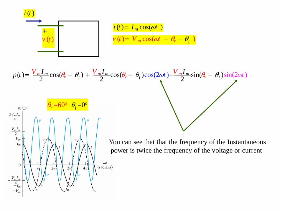
( ) cos( )mi t I tω=

( ) cos( )v imv t V tω θ θ= + −

( ) cos( ) cos( cos() sin( )2 2 2 sin(2 ) 2 )m m mi i

m m mv v v i tI It V Vp V t Iωθ θθ θ θθ ω= − + − − −

o o 0= 0 =6v iθθ

You can see that that the frequency of the Instantaneous power is twice the frequency of the voltage or current

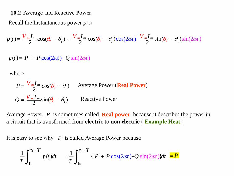
10.2 Average and Reactive Power

( ) cos( ) cos( cos() sin( )2 2 2 sin(2 ) 2 )m m mi i

m m mv v v i tI It V Vp V t Iωθ θθ θ θθ ω= − + − − −

Recall the Instantaneous power p(t)

cos( si( ) ) n ) (2 2p t tt P P Qω ω= + −

where

cos( ) 2 mi

m vIP V θ θ= − Average Power (Real Power)

sin( ) 2 mi

m vIQ V θ θ= − Reactive Power

Average Power P is sometimes called Real power because it describes the power in a circuit that is transformed from electric to non electric ( Example Heat )

It is easy to see why P is called Average Power because

0

0

t +1 ( )t

Tp t dt

T ∫0

0

cos(t +1 sin(2) )

t 2

TP P Q t dt

Ttω ω= + −∫ P=

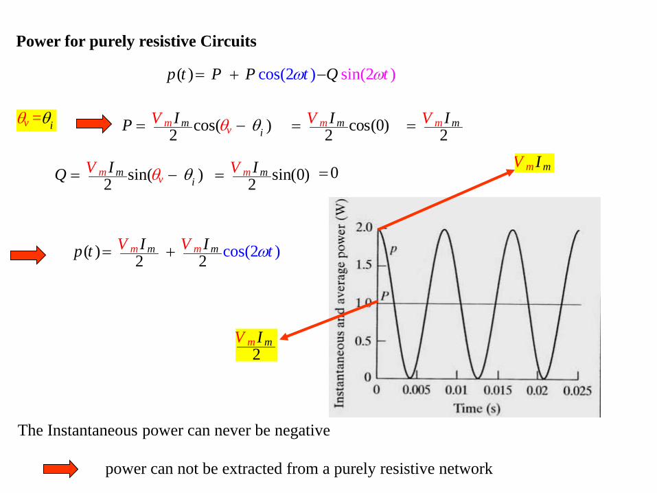
Power for purely resistive Circuits

( ) cos(22 2 )m mm mI Ip t tV V ω= +

= ivθ θ cos( ) 2 mi

m vIP V θ θ= −

sin( ) 2 mi

m vIQ V θ θ= −

2mmV I=

0=

c os(0) 2m mV I=

s in(0) 2m mV I=

The Instantaneous power can never be negative

cos( si( ) ) n ) (2 2p t tt P P Qω ω= + −

mmV I

2mmV I

power can not be extracted from a purely resistive network

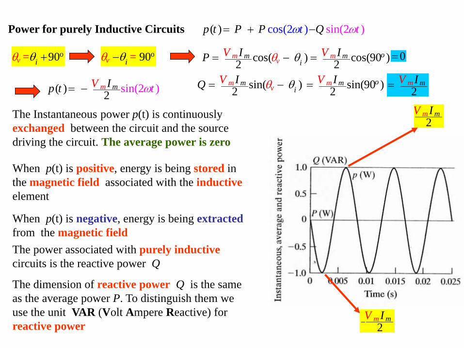
Power for purely Inductive Circuits

sin(2 )( ) 2m mIp Vt tω= −

o9= 0ivθ θ + cos( ) 2 mi

m vIP V θ θ= −

sin( ) 2 mi

m vIQ V θ θ= − 2

mmV I=

0=cos(90 ) 2om mV I=

sin(90 ) 2om mV I=

cos( si( ) ) n ) (2 2p t tt P P Qω ω= + −

2mmV I

2mmV I

−

o= 90 v iθθ −

The Instantaneous power p(t) is continuously exchanged between the circuit and the source driving the circuit. The average power is zero

When p(t) is positive, energy is being stored in the magnetic field associated with the inductive element

When p(t) is negative, energy is being extracted from the magnetic field The power associated with purely inductive circuits is the reactive power Q

The dimension of reactive power Q is the same as the average power P. To distinguish them we use the unit VAR (Volt Ampere Reactive) for reactive power

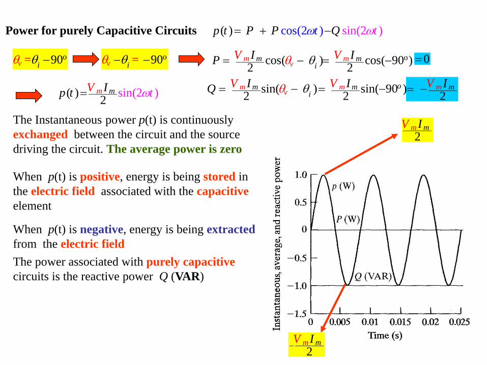
Power for purely Capacitive Circuits

( ) 2 sin(2 )m mV Ip t tω=

o9= 0ivθ θ − cos( ) 2 mi

m vIP V θ θ= −

sin( ) 2 mi

m vIQ V θ θ= − 2

mmV I= −

0=ocos( 9 )2 0 m mIV= −

sin( 9 2 0 )m omIV= −

cos( si( ) ) n ) (2 2p t tt P P Qω ω= + −

2mmV I

2mmV I

−

o= 90v iθθ − −

The Instantaneous power p(t) is continuously exchanged between the circuit and the source driving the circuit. The average power is zero

When p(t) is positive, energy is being stored in the electric field associated with the capacitive element

When p(t) is negative, energy is being extracted from the electric field The power associated with purely capacitive circuits is the reactive power Q (VAR)

The power factor

( ) cos( ) c

s

os( ) sin in( )2 2 2

c (os(2 )

2

)m m mm m miv v vi i

I I Ip t

P P

V tV

Q

t Vθ ωθ θθ θ θω= − + − − −

average averagepower po

reactivepw o erer w

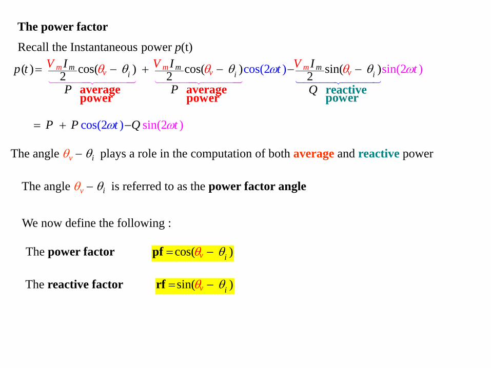
Recall the Instantaneous power p(t)

cos( sin(2 2 ) ) tQtP P ω ω= + −

The angle θv − θi plays a role in the computation of both average and reactive power

The angle θv − θi is referred to as the power factor angle

We now define the following :

The power factor cos( )v iθ θ= −pf

The reactive factor sin( )v iθ θ= −rf

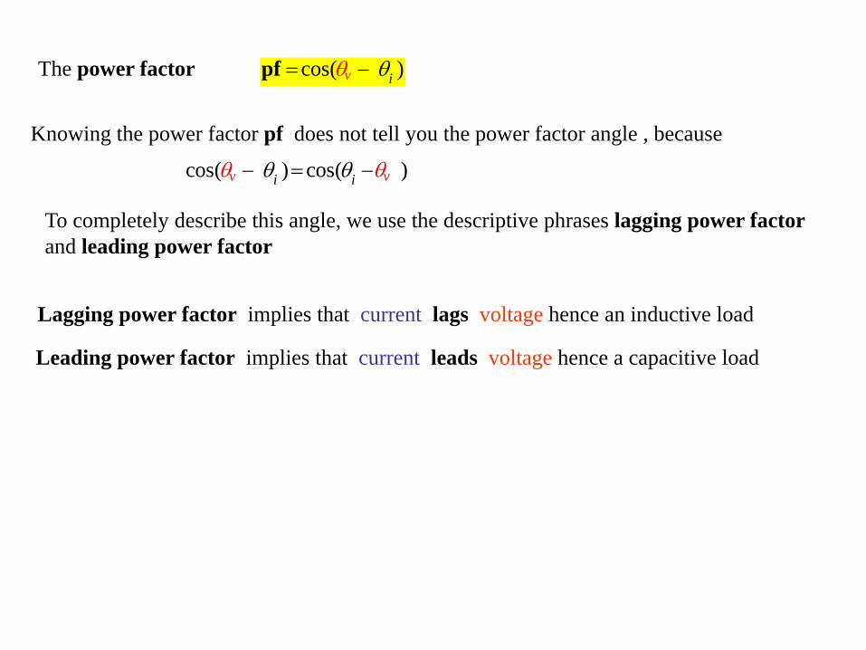
The power factor cos( )v iθ θ= −pf

Knowing the power factor pf does not tell you the power factor angle , because

cos( ) cos( )i viv θ θθ θ− = −

To completely describe this angle, we use the descriptive phrases lagging power factor and leading power factor

Lagging power factor implies that current lags voltage hence an inductive load

Leading power factor implies that current leads voltage hence a capacitive load

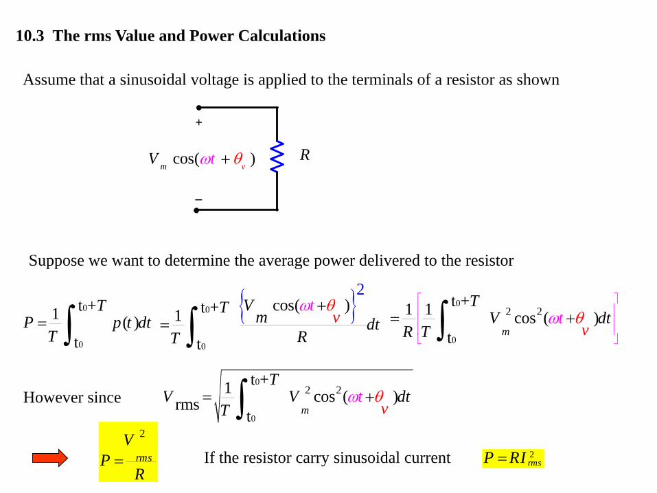
10.3 The rms Value and Power Calculations

R

+

−

cos( )m vV tω θ+

Assume that a sinusoidal voltage is applied to the terminals of a resistor as shown

Suppose we want to determine the average power delivered to the resistor

0

0

t +1 ( )t

TP p t dt

T= ∫

0

0

cos2

( )t +1 t

tv

VT m dtRT

θω += ∫

0

0

2 2t +1 1 cos ( )t m

TV dt

Rt

T vω θ

= +∫

However since 0

0

2 2t +1 cos ( )rms

t m

TV V dt

T vt θω= +∫

2

rmsV

PR

= If the resistor carry sinusoidal current 2rmsP RI=

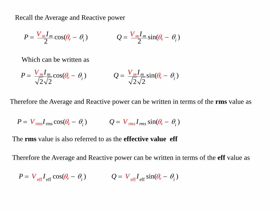
Recall the Average and Reactive power

cos( ) 2 mi

m vIP V θ θ= − sin( ) 2 m

im v

IQ V θ θ= −

Which can be written as

cos( ) 2 2

m v imV IP θ θ= − sin( )

2 2 m v i

mV IQ θ θ= −

Therefore the Average and Reactive power can be written in terms of the rms value as

s rmsrm cos( ) v iP V I θ θ= − sin( ) rms vrms iQ V I θ θ= −

The rms value is also referred to as the effective value eff

Therefore the Average and Reactive power can be written in terms of the eff value as

f effef cos( ) v iP V I θ θ= − f effef sin( ) v iQ V I θ θ= −

Example 10.3

10.4 Complex Power

Previously, we found it convenient to introduce sinusoidal voltage and current in terms of the complex number the phasor

Definition

were is the complex power is the reactive p

is the average poweerr

ow

P

Q

j

P

Q= +S

S

Let the complex power be the complex sum of real power and reactive power

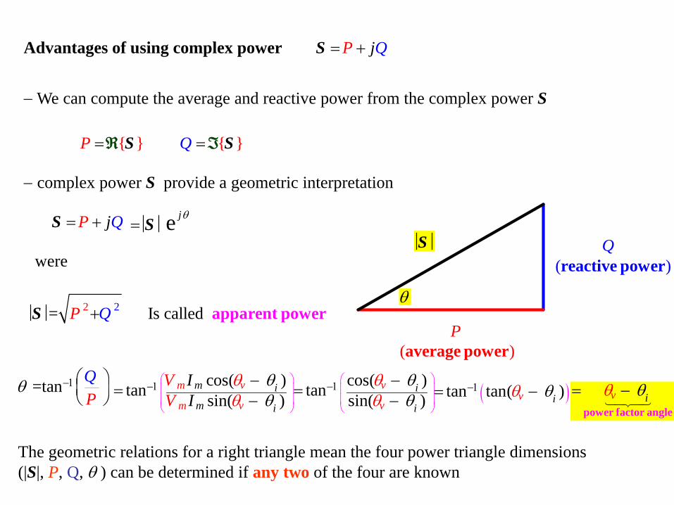
Advantages of using complex power

P = Sℜ Q = Sℑ

− We can compute the average and reactive power from the complex power S

− complex power S provide a geometric interpretation

QjP= +S

QjP= +SS

( )Q

reactive power

( )

Paverage power

θ

cos( )tan sin( )vm

vm

m im i

IVIV

θ θθ θ

−1

−=−

2 2= Is called P Q+ apparent powerS

n =ta QP

θ −1

e jθ= S

were

cos( )tan sin( )v i

iv

θθ

θθ

1

− −=− ( )tan tan( )v iθ θ−1= − iv θθ= −

power factor angle

The geometric relations for a right triangle mean the four power triangle dimensions (|S|, P, Q, θ ) can be determined if any two of the four are known

Example 10.4

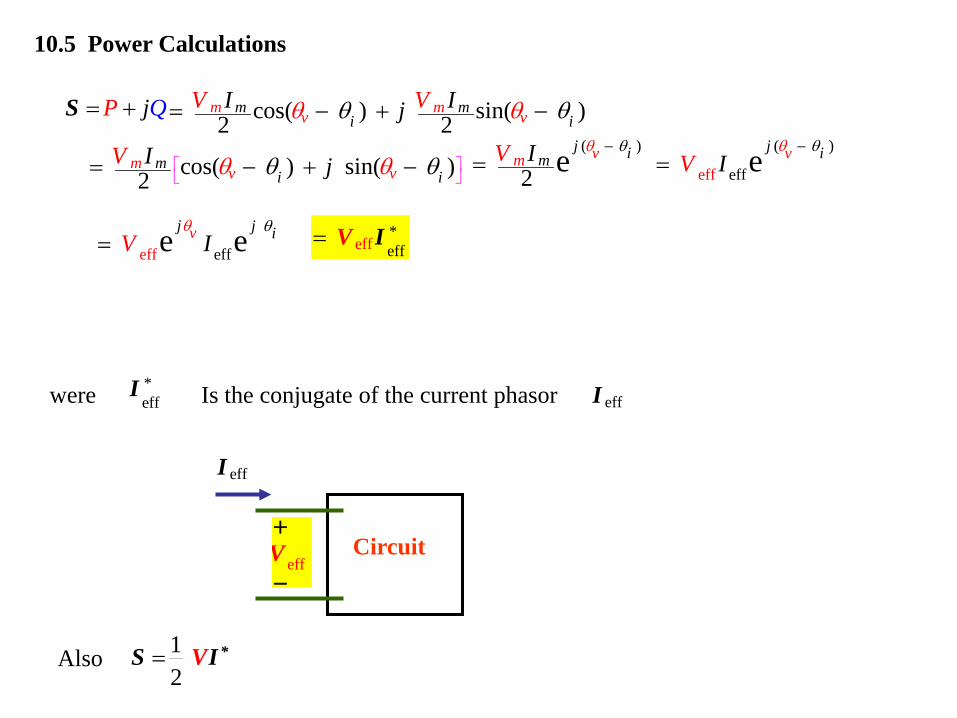
10.5 Power Calculations

QjP= +S cos( ) sin( )2 2 m mi i

m mv vV VI Ijθ θθ θ= − + −

cos( ) sin( )2 m v vmi i

I jV θ θθ θ = − + −

( )

2 e j ivmmV I θ θ−= eff

( )

eff e ivjV I

θ θ−=

eff

eff e evj j iIVθ θ

= eff*eff

= V I

were *eff

I Is the conjugate of the current phasor effI

effV+

−

effI

Circuit

Also 1 2

= *S VI

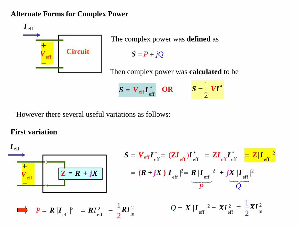
Alternate Forms for Complex Power

effV+

−

effI

Circuit

1 2

= *S VI

eff*eff

=S IV

The complex power was defined as

QjP= +S

Then complex power was calculated to be

OR

However there several useful variations as follows:

First variation

eff*eff

( )= Z II

eff*eff

=S IV

eff*eff

= Z II 2eff

| | = Z I

2eff

| | = ( )+ X IjR

effI

effV+

−Z = +R jX 2 2

eff eff| | | | = + X IjR I

P

Q

2eff

| |P = R I 2eff

I= R 2m

1 2

I= R 2eff

| |Q = X I 2eff

I= X 2m

12

I= X

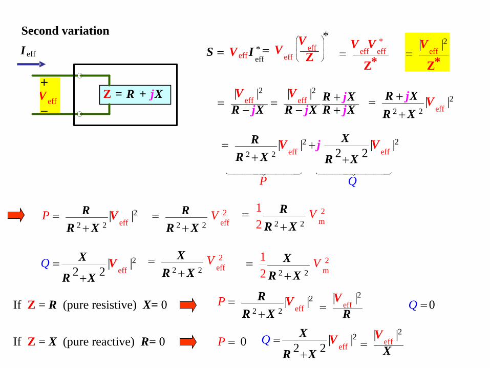
eff*eff

=S IV

Second variation eff

eff

*

= ZV

V*

eff eff =*Z

V Veff

2 | |

=*Z

V

eff2|

|

= −V

R jX

effI

effV+

−Z = +R jX

P

e2

ff | | += − +

jR XVR X Rj jX

22 e2 ff

| |+=+

R XR X

Vj

eff e2 2

2 2 ff | | | |

2 2= +

+ +V Vj XR

R X R X

Q

22 2 eff

| |P =+R X

VR

e2

ff| |

2 2Q =

+VX

R X

2 2

2eff

V=+R

R X2

m

2 2

1 2

V=+R

R X

2 2

2eff

V=+X

R X2

m

2 2

1 2

V=+X

R X

If Z = R (pure resistive) X= 0 22 2 eff

| |P =+R X

VReff

2|

|=

VR

0Q =

If Z = X (pure reactive) R= 0 0P = e2

ff| |

2 2Q =

+VX

R Xeff

2|

|=

VX

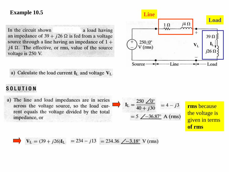
Example 10.5 Line Load

rms because the voltage is given in terms of rms

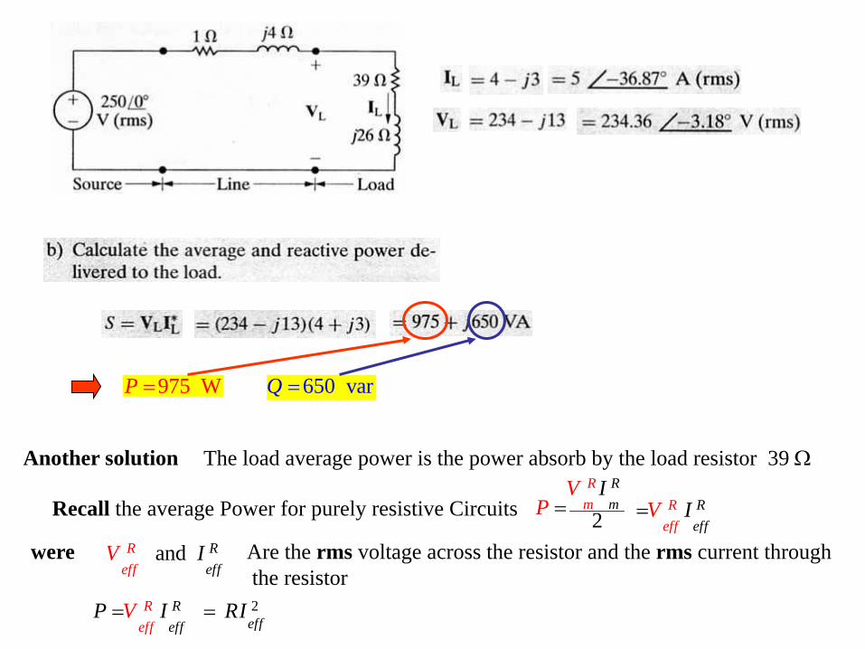
975 WP = 650 varQ =

Another solution The load average power is the power absorb by the load resistor 39 Ω

Recall the average Power for purely resistive Circuits

were and Rf

Reff ef

IV Are the rms voltage across the resistor and the rms current through the resistor 2 eff

RI=

2

R Rm m

VP

I= R

feffRe f

IV=

R Reeff ff

P IV=

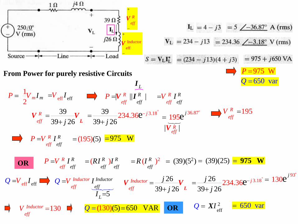
975 WP =650 varQ =

2 (39)(5 )= (39)(25)= = 975 W

| || |Rff ffe

Re

P = IV

3939 26

Reff j

=+ L

V Vo36.87

195e j=

195Reff

V =

R Reeff ff

P IV= (195 ))(5= 975 W=

OR R Reeff ff

P IV= ( )R Reff eff

RI I= 2( )Reff

R I=

o3.18234.39

9 236

3 6e j

j−=

+

5

Inductoreff

Inductoreff

L

Q IV

I

=

=

2639 26

Inductoreff

jj

=+ L

V Vo

3.182342639 6

.362

e jjj

−=+

o93 130e j

=

130Inductoreff

V = (5)(1 630 5 VA) 0 RQ == OR 650 var=2eff

IQ = X

Reff

+

−

V

| | Reff

V

RfeffRe f

IV=

From Power for purely resistive Circuits

2 1 mmP V I= efeff f IV=

LI

eff eff VQ I=

Inductoreff

+

−

V

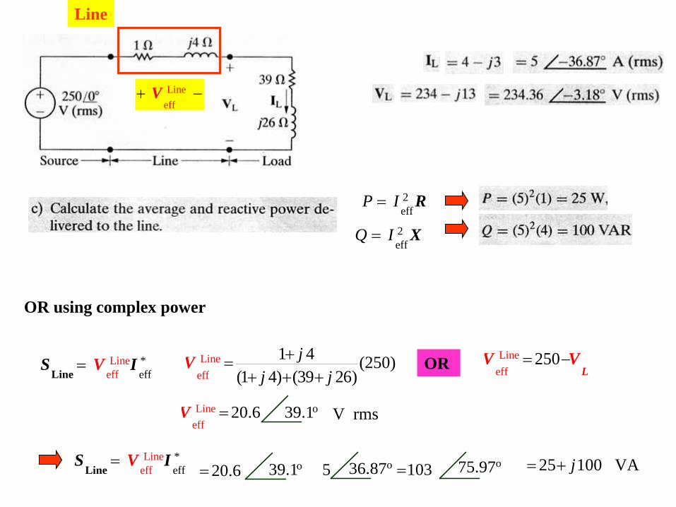
Line

2eff

P I= R

2eff

Q I= X

Lineeff

*eff

=Line

IVS

Lineeff

+ −V

Lineeff

1 4 (250)(1 4) (39 26)

jj j

+=+ + +

V OR Lineeff

250= −L

V V

o39.1Lineeff

20.6=V V rms

Lineeff

*eff

=Line

IVS o39.120.6= o36.875 103= o75.97 25 100 VAj= +

OR using complex power

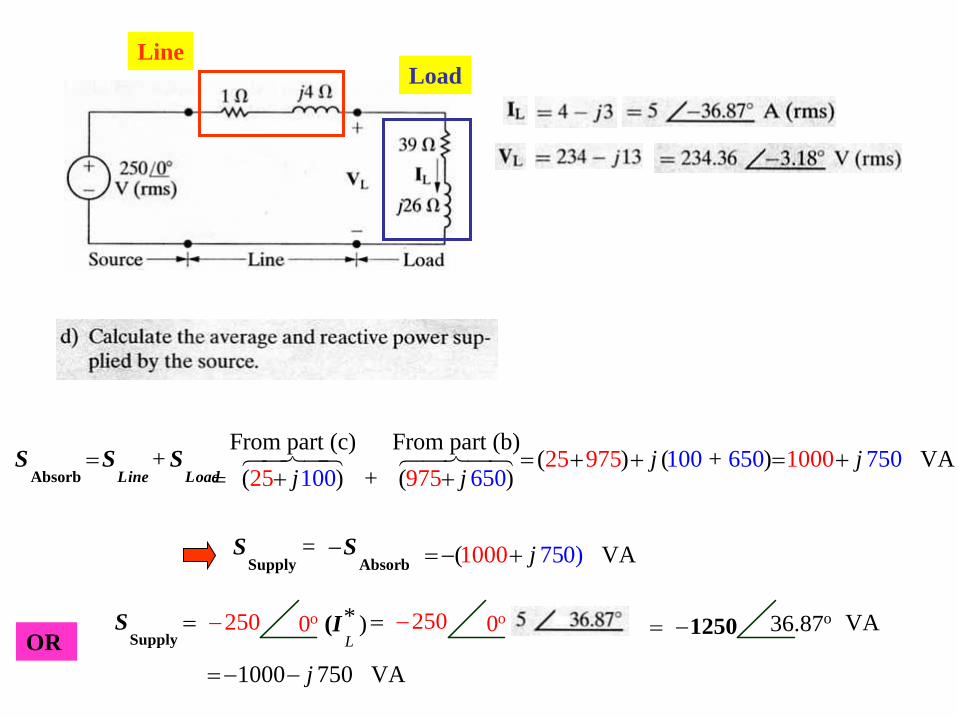
Line Load

+=Absorb Line Load

S S S100

From part (c) From part (b)( ) + ( )25 97 6505j j= + + ( ) (1025 9 07 6 05 )5+ j= + + 751 000 VA0 j= +

OR

7( VA10 0 0 50) j= − += −Supply Absorb

S S

1000 750 VA j= − −

250−=Supply

S o0 )L*(I 250= − o0 = −1250 o36.87 VA

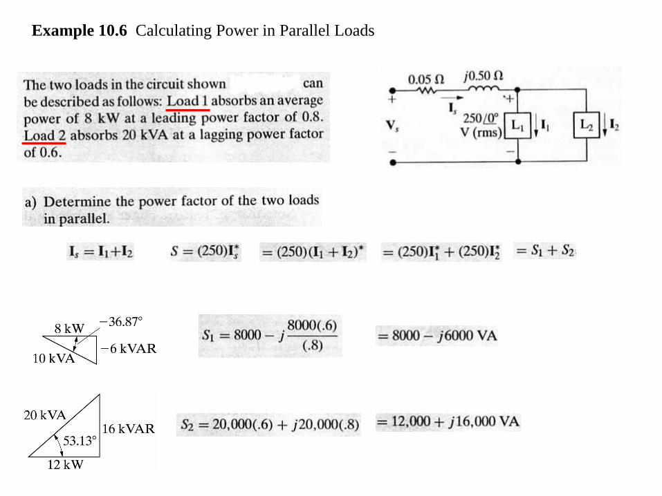
Example 10.6 Calculating Power in Parallel Loads

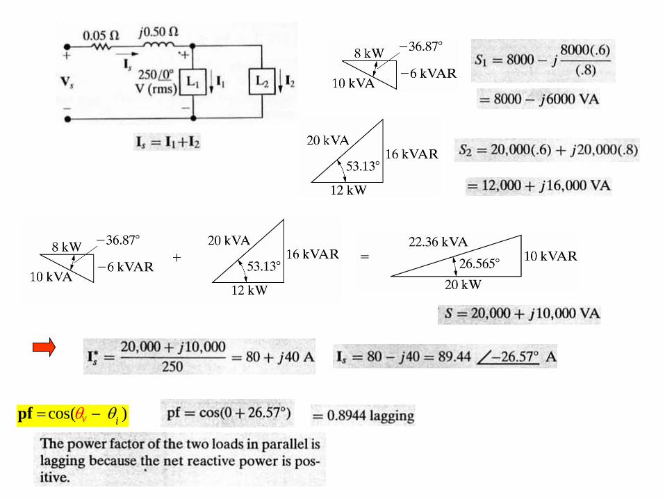
cos( )v iθ θ= −pf

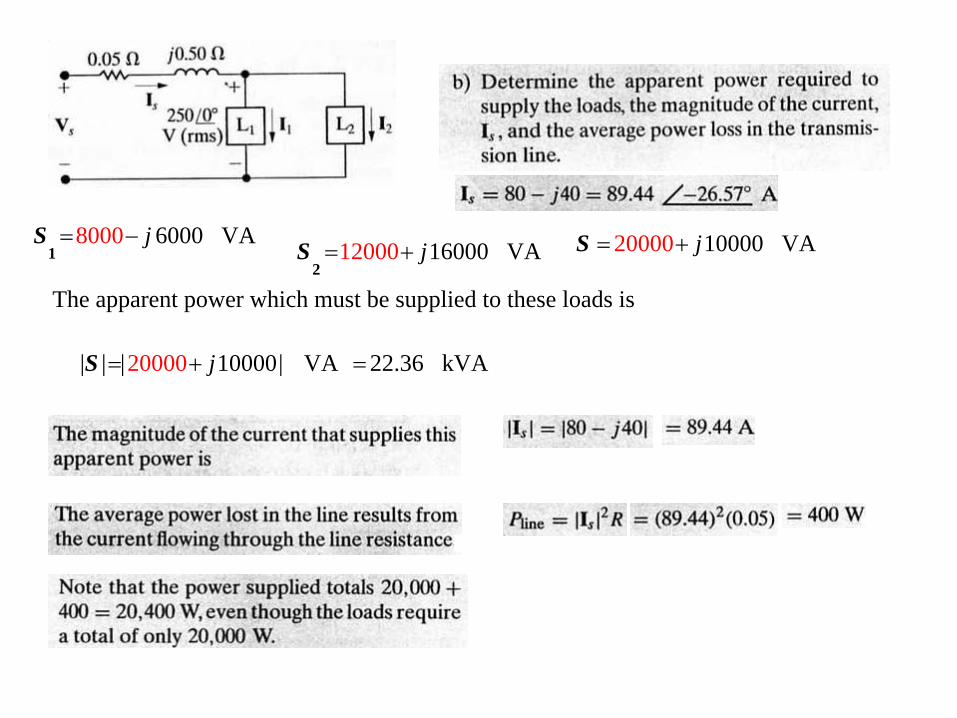
6 000 V 8 A000 j= −1

S1 6000 V 1 A2000 j= +

2S 10000 V2000 0 A j= +S

The apparent power which must be supplied to these loads is

20000| | | 100 VA 00| j= +S 22.36 kVA =

C ?

| |S

As we can see from the power triangle

We can correct the power factor to 1

Recall that 1XCω

= −

if we place a capacitor in parallel with the existing load

Will cancel this

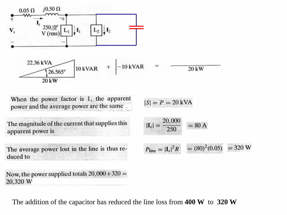
The addition of the capacitor has reduced the line loss from 400 W to 320 W

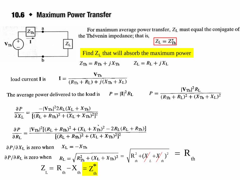
2 2 R ( )th L th

X X= + + th R=

L th th Z R X= −

th*= Z

Find ZL that will absorb the maximum power