You Are Where You Tweet: A Content-Based Approach to …faculty.cs.tamu.edu/caverlee/pubs/cheng10cikm.pdf · You Are Where You Tweet: A Content-Based Approach to Geo-locating Twitter

You Are Where You Tweet: A Content-Based Approach toGeo-locating Twitter Users

Zhiyuan ChengDepartment of ComputerScience and Engineering

Texas A&M UniversityCollege Station, TX, USA

[email protected]

James CaverleeDepartment of ComputerScience and Engineering

Texas A&M UniversityCollege Station, TX, USA

[email protected]

Kyumin LeeDepartment of ComputerScience and Engineering

Texas A&M UniversityCollege Station, TX, USA

[email protected]

ABSTRACTWe propose and evaluate a probabilistic framework for es-timating a Twitter user’s city-level location based purelyon the content of the user’s tweets, even in the absenceof any other geospatial cues. By augmenting the massivehuman-powered sensing capabilities of Twitter and relatedmicroblogging services with content-derived location infor-mation, this framework can overcome the sparsity of geo-enabled features in these services and enable new location-based personalized information services, the targeting of re-gional advertisements, and so on. Three of the key featuresof the proposed approach are: (i) its reliance purely on tweetcontent, meaning no need for user IP information, privatelogin information, or external knowledge bases; (ii) a clas-sification component for automatically identifying words intweets with a strong local geo-scope; and (iii) a lattice-basedneighborhood smoothing model for refining a user’s locationestimate. The system estimates k possible locations for eachuser in descending order of confidence. On average we findthat the location estimates converge quickly (needing just100s of tweets), placing 51% of Twitter users within 100miles of their actual location.

Categories and Subject Descriptors: H.2.8 [DatabaseManagement]: Database applications–Data mining; J.4[Computer Application]: Social and Behavioral Sciences

General Terms: Algorithms, Experimentation

Keywords: Twitter, location-based estimation, spatial datamining, text mining

1. INTRODUCTIONThe rise of microblogging services like Twitter has spawned

great interest in these systems as human-powered sensingnetworks. Since its creation in 2006, Twitter has experi-enced an exponential explosion in its user base, reaching

Permission to make digital or hard copies of all or part of this work forpersonal or classroom use is granted without fee provided that copies arenot made or distributed for profit or commercial advantage and that copiesbear this notice and the full citation on the first page. To copy otherwise, torepublish, to post on servers or to redistribute to lists, requires prior specificpermission and/or a fee.CIKM’10, October 26–30, 2010, Toronto, Ontario, Canada.Copyright 2010 ACM 978-1-4503-0099-5/10/10 ...$10.00.

approximately 75 million users as of 2010 [4]. These usersactively publish short messages (“tweets”) of 140 charactersor less to an audience of their subscribers (“followers”). Withsuch a large geographically diverse user base, Twitter hasessentially published terabytes of real-time “sensor” data inthe form of these status updates.

Mining this people-centric sensor data promises new per-sonalized information services, including local news summa-rized from tweets of nearby Twitter users [21], the target-ing of regional advertisements, spreading business informa-tion to local customers [3], and novel location-based applica-tions (e.g., Twitter-based earthquake detection, which canbe faster than through traditional official channels [18]).

Unfortunately, Twitter users have been slow to adopt geospa-tial features: in a random sample of over 1 million Twitterusers, only 26% have listed a user location as granular asa city name (e.g., Los Angeles, CA); the rest are overlygeneral (e.g., California), missing altogether, or nonsensical(e.g., Wonderland). In addition, Twitter began supportingper-tweet geo-tagging in August 2009. Unlike user location(which is a single location associated with a user and listedin each Twitter user’s profile), this per-tweet geo-taggingpromises extremely fine-tuned Twitter user tracking by as-sociating each tweet with a latitude and longitude. Oursample shows, however, that fewer than 0.42% of all tweetsactually use this functionality. Together, the lack of useradoption of geo-based features per user or per tweet signalsthat the promise of Twitter as a location-based sensing sys-tem may have only limited reach and impact.

To overcome this location sparsity problem, we proposein this paper to predict a user’s location based purely onthe content of the user’s tweets, even in the absence of anyother geospatial cues. Our intuition is that a user’s tweetsmay encode some location-specific content – either specificplace names or certain words or phrases more likely to beassociated with certain locations than others (e.g., “howdy”for people from Texas). In this way, we can fill-the-gap forthe 74% of Twitter users lacking city-level granular locationinformation. By augmenting the massive human-poweredsensing capabilities of Twitter and related microbloggingservices with content-derived location information, this frame-work can overcome the sparsity of geo-enabled features inthese services and bring augmented scope and breadth toemerging location-based personalized information services.

Effectively geo-locating a Twitter user based purely onthe content of their tweets is a difficult task, however:

• First, Twitter status updates are inherently noisy, mix-

ing a variety of daily interests (e.g., food, sports, dailychatting with friends). Are there clear location signalsembedded in this mix of topics and interests that can beidentified for locating a user?

• Second, Twitter users often rely on shorthand and non-standard vocabulary for informal communication, mean-ing that traditional gazetteer terms and proper placenames (e.g., Eiffel Tower) may not be present in the con-tent of the tweets at all, making the task of determiningwhich terms are location-sensitive non-trivial.

• Third, even if we could isolate the location-sensitive at-tributes of a user’s tweets, a user may have interests thatspan multiple locations beyond their immediate home lo-cation, meaning that the content of their tweets may beskewed toward words and phrase more consistent withoutside locations. For example, New Yorkers may postabout NBA games in Los Angeles or the earthquake inHaiti.

• Fourth, a user may have more than one associated lo-cation, e.g., due to travel, meaning that content-basedlocation estimation may have difficulty in precisely iden-tifying a user’s location.

As a consequence, it is challenging to estimate the real lo-cation for a Twitter user based on an analysis of the user’stweets. With these issues in mind, in this paper, we pro-pose and evaluate a probabilistic framework for estimatinga Twitter user’s city-level location based purely on the con-tent of the user’s tweets. The proposed approach relies onthree key features: (i) its data input of pure tweet content,without any external data from users or web-based knowl-edge bases; (ii) a classifier which identifies words in tweetswith a local geographic scope; and (iii) a lattice-based neigh-borhood smoothing model for refining the estimated results.The system provides k estimated cities for each user witha descending order of possibility. On average, 51% of ran-domly sampled Twitter users are placed within 100 miles oftheir actual location (based on an analysis of just 100s oftweets). We find that increasing amounts of data (in theform of wider coverage of Twitter users and their associatedtweets) results in more precise location estimation, givingus confidence in the robustness and continued refinement ofthe approach.

The rest of this paper is organized as follows: Relatedwork is in Section 2. Section 3 formalizes the problem ofpredicting a Twitter user’s geo-location and briefly describesthe sampled Twitter dataset used in the experiments. InSection 4, our estimation algorithm and corresponding re-finements are introduced. We present the experimental re-sults in Section 5. Finally, conclusions and future work arediscussed in Section 6.

2. RELATED WORKStudying the geographical scope of online content has at-

tracted attention by researchers in the last decade, includingstudies of blogs [11, 15], webpages [7], search engine querylogs [8], and even web users [13]. Prior work relevant to thispaper can be categorized roughly into three groups based onthe techniques used in geo-locating: content analysis withterms in a gazetteer, content analysis with probabilistic lan-guage models, and inference via social relations.

Several studies try to estimate the location of web con-tent utilizing content analysis based on geo-related terms in

a specialized external knowledge base (a gazetteer). Ami-tay et al. [7], Fink et al. [11], and Zong et al. [22] ex-tracted addresses, postal code, and other information listedin a geographical gazetteer from web content to identify theassociated geographical scope of web pages and blogs.

Serdyukov et al. [19] generate probabilistic language mod-els based on the tags that photos are labeled with by Flickrusers. Based on these models and Bayesian inference, theyshow how to estimate the location for a photo. In terms ofthe intention, their method is similar to our work. However,they use a GeoNames database to decide whether a user-submitted tag is a geo-related tag, which can overlook thespatial usefulness of words that may have a strong geo-scope(e.g., earthquake, casino, and so on). Separately, the work ofCrandall et al. [10] proposes an approach combining textualand visual features to place images on a map. They haverestrictions in their task that their system focuses on whichof ten landmarks in a given city is the scope of an image.

In the area of privacy inference, a few researchers havebeen studying how a user’s private information may be in-ferred through an analysis of the user’s social relations. Back-strom et al. [9], Lindamood et al. [16], and Hearthely etal. [12] all share a similar assumption that users relatedin social networks usually share common attributes. Thesemethods are orthogonal to our effort and could be used toaugment the content-based approach taken in this paper byidentifying common locations among a Twitter user’s socialnetwork.

Recent work on detecting earthquakes with real-time Twit-ter data makes use of location information for tracking theflow of information across time and space [18]. Sakaki et al.consider each Twitter user as a sensor and apply Kalmanfiltering and particle filtering to estimate the center of thebursty earthquake. Their algorithm requires prior knowl-edge of where and when the earthquake is reported, empha-sizing tracking instead of geo-locating users. As a result, thisand related methods could benefit from our efforts to assignlocations to users for whom we have no location information.

3. PRELIMINARIESIn this section, we briefly explain our dataset, formalize

the research problem and describe the experimental setup.

3.1 Location Sparsity on TwitterTo derive a representative sample of Twitter users, we

employed two complementary crawling strategies: crawl-ing through Twitter’s public timeline API and crawling bybreadth-first search through social edges to crawl each user’sfriends (following) and followers. The first strategy can beconsidered as random sampling from active Twitter users(whose tweets are selected for the public timeline), whilethe second strategy extracts a directed acyclic sub-graph ofthe whole Twitter social graph, including less active Twit-ter users. We combine the two strategies to avoid bias ineither one. Using the open-source library twitter4j [5] to ac-cess Twitter’s open API [6] from September 2009 to January2010, we collected a base dataset of 1,074,375 user profilesand 29,479,600 status updates.

Each user profile includes the capacity to list the user’sname, location, a web link, and a brief biography. We findthat 72.05% of the profiles collected do list a non-emptylocation, including locations like “Hollywood, CA”, “Eng-land”, and “UT: 40.708046,-73.789259”. However, we find

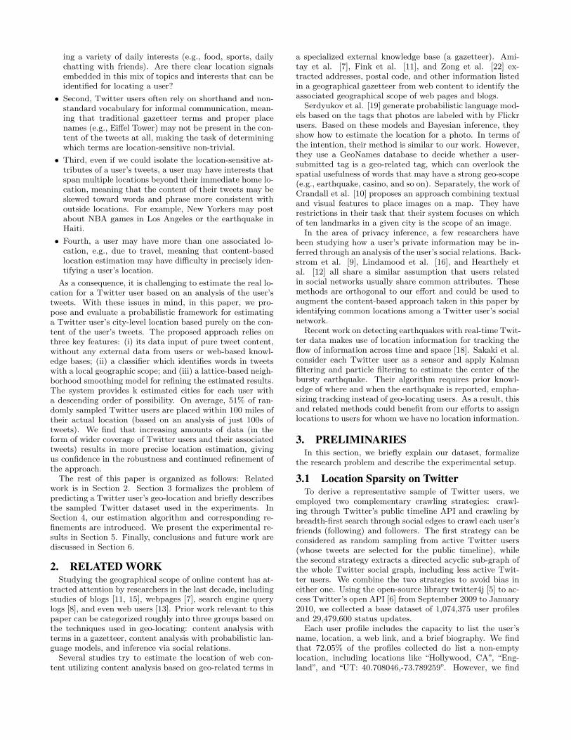
(a) Population Distribution of the Continental United States (b) User Distribution of Sampled Twitter Dataset

Figure 1: Comparison Between the Actual US Population and the Sample Twitter User Population

that most of these user-submitted locations are overly gen-eral with a wide geographic scope (e.g., California, world-wide), missing altogether, or nonsensical (e.g., Wonderland,“CALI to FORNIA”). Specifically, we examine all locationslisted in the 1,074,375 user profiles and find that just 223,418(21% of the total) list a location as granular as a city nameand that only 61,335 (5%) list a location as granular as alatitude/longitude coordinate. This absence of granular lo-cation information for the majority of Twitter users (74%)indicates the great potential in estimating or recommendinglocation for a Twitter user.

For the rest of the paper, we focus our study of Twit-ter user location estimation on users within the continen-tal United States. Toward this purpose, we filter all listedlocations that have a valid city-level label in the form of“cityName”, “cityName, stateName”, and “cityName, state-Abbreviation”, where we consider all valid cities listed inthe Census 2000 U.S. Gazetteer [1] from the U.S. CensusBureau. Even when considering these data forms, there canstill be ambiguity for cities listed using just“cityName”, e.g.,there are three cities named Anderson, four cities named Ar-lington, and six cities called Madison. For these ambiguouscases, we only consider cities listed in the form “cityName,stateName”, and “cityName, stateAbbreviation”. After ap-plying this filter, we find that there are 130,689 users (with4,124,960 status updates), accounting for 12% of all sampledTwitter users. This sample of Twitter users is representa-tive of the actual population of the United States as can beseen in Figure 1(a), and Figure 1(b).

3.2 Problem StatementGiven the lack of granular location information for Twit-

ter users, our goal is to estimate the location of a user basedpurely on the content of their tweets. Having a reasonableestimate of a user’s location can enable content personaliza-tion (e.g., targeting advertisements based on the user’s geo-graphical scope, pushing related news stories, etc.), targetedpublic health web mining (e.g., a Google Flu Trends-likesystem that analyzes tweets for regional health monitoring),and local emergency detection (e.g., detecting emergenciesby monitoring tweets about earthquakes, fires, etc.). Byfocusing on the content of a user’s Twitter stream, such anapproach can avoid the need for private user information, IPaddress, or other sensitive data. With these goals in mind,

we focus on city-level location estimation for a Twitter user,where the problem can be formalized as:

Location Estimation Problem: Given a set of tweetsStweets(u) posted by a Twitter user u, estimate a user’sprobability of being located in city i: p(i|Stweets(u)), suchthat the city with maximum probability lest(u) is the user’sactual location lact(u).

As we have noted, location estimation based on tweet con-tent is a difficult and challenging problem. Twitter statusupdates are inherently noisy, often relying on shorthand andnon-standard vocabulary. It is not obvious that there areclear location cues embedded in a user’s tweets at all. Auser may have interests which span multiple locations anda user may have more than one natural location.

3.3 Evaluation Setup and MetricsToward developing a content-based user location estima-

tor, we next describe our evaluation setup and introducefour metrics to help us evaluate the quality of a proposedestimator.

Test Data: In order to be fair in our evaluation of thequality of location estimation, we build a test set that isseparate from the 130,689 users previously identified (andthat will be used for building our models for predicting userlocation). In particular, we extract a set of active users with1000+ tweets who have listed their location in the form oflatitude/longitude coordinates. Since these types of user-submitted locations are typically generated by smartphones,we assume these locations are correct and can be used asground truth. We filter out spammers, promoters, and otherautomated-script style Twitter accounts using features de-rived from Lee et al.’s work [14] on Twitter bot detection, sothat the test set will consist of primarily “regular” Twitterusers for whom location estimation would be most valuable.Finally, we arrive at 5,190 test users and more than 5 millionof their tweets. These test users are distributed across thecontinental United States similar to the distributions seenin Figure 1(a), and Figure 1(b).

Metrics: To evaluate the quality of a location estimator, wecompare the estimated location of a user versus the actualcity location (which we know based on the city correspond-ing to their latitude/longitude coordinates). The first metricwe consider is the Error Distance which quantifies the dis-

tance in miles between the actual location of the user lact(u)and the estimated location lest(u). The Error Distance foruser u is defined as:

ErrDist(u) = d(lact(u), lest(u))

To evaluate the overall performance of a content-baseduser location estimator, we further define the Average Er-ror Distance across all test users U :

AvgErrDist(U) =

∑u∈U ErrDist(u)

|U |A low Average Error Distance means that the system cangeo-locate users close to their real location on average, but itdoes not give strong insight into the distribution of locationestimation errors. Hence, the next metric – Accuracy –considers the percentage of users with their error distancecategorized in the range of 0-100 miles:

Accuracy(U) =|{u|u ∈ U ∧ ErrDist(u) ≤ 100}|

|U |Further, since the location estimator predicts k cities for

each user in decreasing order of confidence, we define theAccuracy with K Estimations (Accuracy@k) whichapplies the same Accuracy metric, but over the city in thetop-k with the least error distance to the actual location. Inthis way, the metric shows the capacity of an estimator toidentify a good candidate city, even if the first prediction isin error.

4. CONTENT-BASED LOCATION ESTIMA-TION: OVERVIEW AND APPROACH

In this section, we begin with an overview of our base-line approach for content-based location estimation and thenpresent two key optimizations for improving and refining thequality of location estimates.

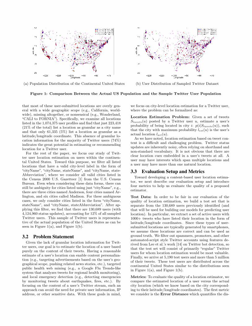
Baseline Location Estimation: First, we can directlyobserve the actual distribution across cities for each wordin the sampled dataset. Based on maximum likelihood es-timation, the probabilistic distribution over cities for wordw can be formalized as p(i|w) which identifies for each wordw the likelihood that it was issued by a user located in cityi. For example, for the word “rockets”, we can see its citydistribution in Figure 2 based on the tweets in the sampleddataset (with a large peak near Houston, home of NASAand the NBA basketball team Rockets).

Of course users from cities other than Houston may tweetthe word “rockets”, so reliance on a single word or a singletweet will necessarily reveal very little information about thetrue location of a user. By aggregating across all words intweets posted by a particular user, however, our intuitionis that the location of the user will become clear. Giventhe set of words Swords(u) extracted from a user’s tweetsStweets(u), we propose to estimate the probability of theuser being located in city i as:

p(i|Swords(u)) =∑

w∈Swords(u)

p(i|w) ∗ p(w)

where we use p(w) to denote the probability of the word win the whole dataset. Letting count(w) be the number of oc-currences of the word w, and t be the total number of tokens

Figure 2: City estimates for the term “rockets”

in the corpus, we replace p(w) with count(w)t

in calculatingthe value of p(w). Such an approach will produce a per-usercity probability across all cities. The city with the highestprobability can be taken as the user’s estimated location.This location estimator is formalized in Algorithm 1.

Algorithm 1 Content-Based User Location Estimation

Input:tweets: List of n tweets from a Twitter user ucityList: Cities in continental US with 5k+ peopledistributions: Probabilistic distributions for wordsk: Number of estimations for each userOutput:estimatedCities: Top K estimations

1: words = preProcess(tweets)2: for city in cityList do3: prob[city]← 04: for word in words do5: prob[city]+ =

distributions[word][city] ∗ word.count6: end for7: end for8: estimatedCities = sort(prob, cityList, k)9: return estimatedCities

Initial Results: Using this baseline approach, we esti-mated the location of all users in our test set using per-cityword distributions estimated from the 130,689 users shownin Figure 1(b). For each user, we parsed their location andstatus updates (4,124,960 in all). In parsing the tweets, weeliminate all occurrences of a standard list of 319 stop words,as well as screen names (which start with @), hyperlinks, andpunctuation in the tweets. Instead of using stemming, weuse the Jaccard Coefficient to check whether a newly encoun-tered word is a variation of a previously encountered word.The Jaccard Coefficient is particularly helpful in handlinginformal content like in tweets, e.g., by treating “awesoome”and “awesooome” as the word “awesome”. In generating theword distributions, we only consider words that occur atleast 50 times in order to build comparatively accurate mod-els. Thus, 25,987 per-city word distributions are generatedfrom a base set of 481,209 distinct words.

Disappointingly, only 10.12% of the 5,119 users in the

test set are geo-located within 100 miles to their real lo-cations and the AvgErrDist is 1,773 miles, meaning thatsuch a baseline content-based location estimator provideslittle value. On inspection, we discovered two key problems:(i) most words are distributed consistently with the popula-tion across different cities, meaning that most words providevery little power at distinguishing the location of a user; and(ii) most cities, especially with a small population, have asparse set of words in their tweets, meaning that the per-cityword distributions for these cities are underspecified leadingto large estimation errors.

In the rest of this section, we address these two problemsin turn in hopes of developing a more valuable and refinedlocation estimator. Concretely, we pursue two directions:

• Identifying Local Words in Tweets: Is there a subset ofwords which have a more compact geographical scopecompared to other words in the dataset? And can these“local” words be discovered from the content of tweets?By removing noise words and non-local words, we may beable to isolate words that can distinguish users locatedin one city versus another.

• Overcoming Tweet Sparsity: In what way can we over-come the location sparsity of words in tweets? By explor-ing approaches for smoothing the distributions of words,can we improve the quality of user location estimationby assigning non-zero probability for words to be issuedfrom cities in which we have no word observations?

4.1 Identifying Local Words in TweetsOur first challenge is to filter the set of words considered

by the location estimation algorithm (Algorithm 1) to con-sider primarily words that are essentially “local”. By con-sidering all words in the location estimator, we saw howthe performance suffers due to the inclusion of noise wordsthat do not convey a strong sense of location (e.g., “august”,“peace”, “world”). By observation and intuition, some wordsor phrases have a more compact geographical scope. Forexample, “howdy” which is a typical greeting word in Texasmay give the estimator a hint that the user is in or nearTexas.

Toward the goal of improving user location estimation, wecharacterize the task of identifying local words as a decisionproblem. Given a word, we must decide if it is local or non-local. Since tweets are essentially informal communication,we find that relying on formally defined location names ina gazetteer is neither scalable nor provides sufficient cov-erage. That is, Twitter’s 140 character length restrictionmeans that users may not write the full address or locationname (e.g., “t-center” instead of “Houston Toyota Center”,home of the NBA Rockets team. Concretely, we propose todetermine local words using a model-driven approach basedon the observed geographical distribution of the words intweets.

4.1.1 Determining Spatial Focus and DispersionIntuitively, a local word is one with a high local focus and

a fast dispersion, that is it is very frequent at some centralpoint (like say in Houston) and then drops off in use rapidlyas we move away from the central point. Non-local words,on the other hand, may have many multiple central pointswith no clear dispersion (e.g., words like basketball). Howdo we assess the spatial focus and dispersion of words intweets?

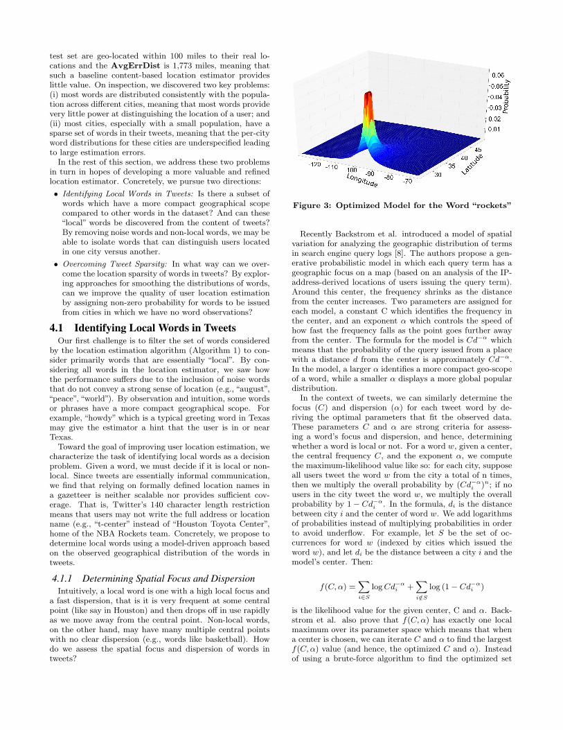
Figure 3: Optimized Model for the Word “rockets”

Recently Backstrom et al. introduced a model of spatialvariation for analyzing the geographic distribution of termsin search engine query logs [8]. The authors propose a gen-erative probabilistic model in which each query term has ageographic focus on a map (based on an analysis of the IP-address-derived locations of users issuing the query term).Around this center, the frequency shrinks as the distancefrom the center increases. Two parameters are assigned foreach model, a constant C which identifies the frequency inthe center, and an exponent α which controls the speed ofhow fast the frequency falls as the point goes further awayfrom the center. The formula for the model is Cd−α whichmeans that the probability of the query issued from a placewith a distance d from the center is approximately Cd−α.In the model, a larger α identifies a more compact geo-scopeof a word, while a smaller α displays a more global populardistribution.

In the context of tweets, we can similarly determine thefocus (C) and dispersion (α) for each tweet word by de-riving the optimal parameters that fit the observed data.These parameters C and α are strong criteria for assess-ing a word’s focus and dispersion, and hence, determiningwhether a word is local or not. For a word w, given a center,the central frequency C, and the exponent α, we computethe maximum-likelihood value like so: for each city, supposeall users tweet the word w from the city a total of n times,then we multiply the overall probability by (Cd−αi )n; if nousers in the city tweet the word w, we multiply the overallprobability by 1− Cd−αi . In the formula, di is the distancebetween city i and the center of word w. We add logarithmsof probabilities instead of multiplying probabilities in orderto avoid underflow. For example, let S be the set of oc-currences for word w (indexed by cities which issued theword w), and let di be the distance between a city i and themodel’s center. Then:

f(C,α) =∑i∈S

logCd−αi +∑i/∈S

log (1− Cd−αi )

is the likelihood value for the given center, C and α. Back-strom et al. also prove that f(C,α) has exactly one localmaximum over its parameter space which means that whena center is chosen, we can iterate C and α to find the largestf(C,α) value (and hence, the optimized C and α). Insteadof using a brute-force algorithm to find the optimized set

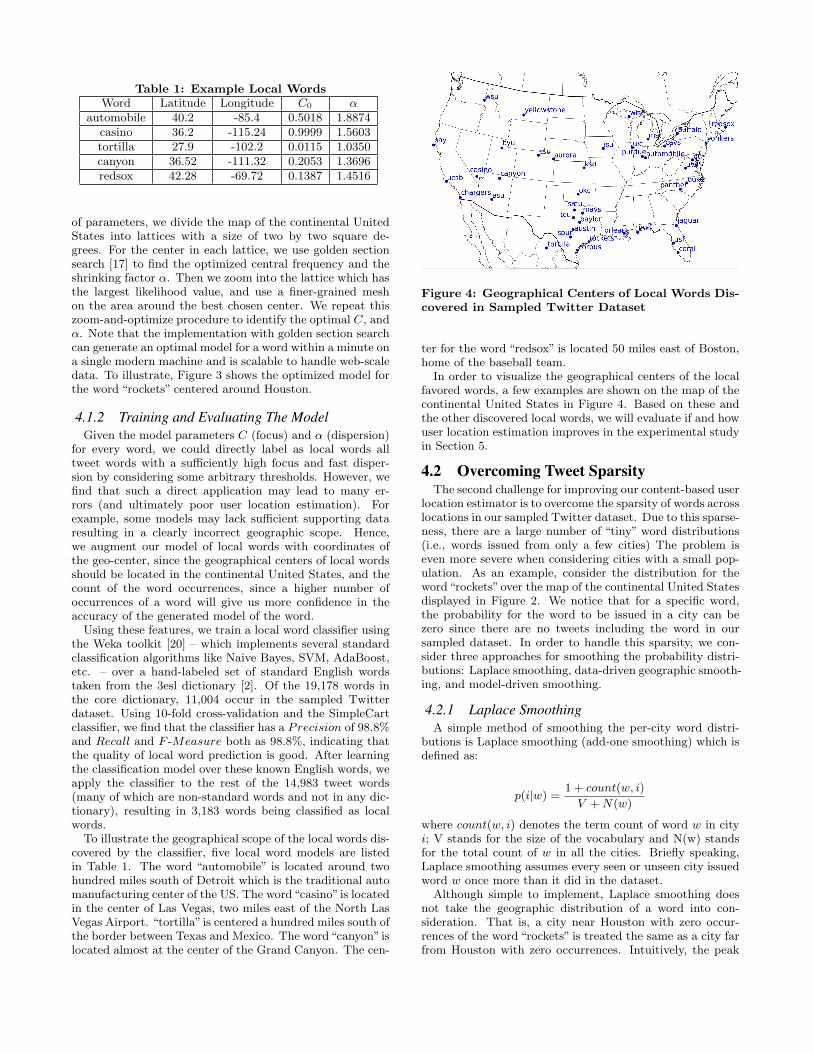
Table 1: Example Local WordsWord Latitude Longitude C0 α

automobile 40.2 -85.4 0.5018 1.8874casino 36.2 -115.24 0.9999 1.5603tortilla 27.9 -102.2 0.0115 1.0350canyon 36.52 -111.32 0.2053 1.3696redsox 42.28 -69.72 0.1387 1.4516

of parameters, we divide the map of the continental UnitedStates into lattices with a size of two by two square de-grees. For the center in each lattice, we use golden sectionsearch [17] to find the optimized central frequency and theshrinking factor α. Then we zoom into the lattice which hasthe largest likelihood value, and use a finer-grained meshon the area around the best chosen center. We repeat thiszoom-and-optimize procedure to identify the optimal C, andα. Note that the implementation with golden section searchcan generate an optimal model for a word within a minute ona single modern machine and is scalable to handle web-scaledata. To illustrate, Figure 3 shows the optimized model forthe word “rockets” centered around Houston.

4.1.2 Training and Evaluating The ModelGiven the model parameters C (focus) and α (dispersion)

for every word, we could directly label as local words alltweet words with a sufficiently high focus and fast disper-sion by considering some arbitrary thresholds. However, wefind that such a direct application may lead to many er-rors (and ultimately poor user location estimation). Forexample, some models may lack sufficient supporting dataresulting in a clearly incorrect geographic scope. Hence,we augment our model of local words with coordinates ofthe geo-center, since the geographical centers of local wordsshould be located in the continental United States, and thecount of the word occurrences, since a higher number ofoccurrences of a word will give us more confidence in theaccuracy of the generated model of the word.

Using these features, we train a local word classifier usingthe Weka toolkit [20] – which implements several standardclassification algorithms like Naive Bayes, SVM, AdaBoost,etc. – over a hand-labeled set of standard English wordstaken from the 3esl dictionary [2]. Of the 19,178 words inthe core dictionary, 11,004 occur in the sampled Twitterdataset. Using 10-fold cross-validation and the SimpleCartclassifier, we find that the classifier has a Precision of 98.8%and Recall and F -Measure both as 98.8%, indicating thatthe quality of local word prediction is good. After learningthe classification model over these known English words, weapply the classifier to the rest of the 14,983 tweet words(many of which are non-standard words and not in any dic-tionary), resulting in 3,183 words being classified as localwords.

To illustrate the geographical scope of the local words dis-covered by the classifier, five local word models are listedin Table 1. The word “automobile” is located around twohundred miles south of Detroit which is the traditional automanufacturing center of the US. The word“casino”is locatedin the center of Las Vegas, two miles east of the North LasVegas Airport. “tortilla” is centered a hundred miles south ofthe border between Texas and Mexico. The word“canyon” islocated almost at the center of the Grand Canyon. The cen-

Figure 4: Geographical Centers of Local Words Dis-covered in Sampled Twitter Dataset

ter for the word “redsox” is located 50 miles east of Boston,home of the baseball team.

In order to visualize the geographical centers of the localfavored words, a few examples are shown on the map of thecontinental United States in Figure 4. Based on these andthe other discovered local words, we will evaluate if and howuser location estimation improves in the experimental studyin Section 5.

4.2 Overcoming Tweet SparsityThe second challenge for improving our content-based user

location estimator is to overcome the sparsity of words acrosslocations in our sampled Twitter dataset. Due to this sparse-ness, there are a large number of “tiny” word distributions(i.e., words issued from only a few cities) The problem iseven more severe when considering cities with a small pop-ulation. As an example, consider the distribution for theword“rockets”over the map of the continental United Statesdisplayed in Figure 2. We notice that for a specific word,the probability for the word to be issued in a city can bezero since there are no tweets including the word in oursampled dataset. In order to handle this sparsity, we con-sider three approaches for smoothing the probability distri-butions: Laplace smoothing, data-driven geographic smooth-ing, and model-driven smoothing.

4.2.1 Laplace SmoothingA simple method of smoothing the per-city word distri-

butions is Laplace smoothing (add-one smoothing) which isdefined as:

p(i|w) =1 + count(w, i)

V +N(w)

where count(w, i) denotes the term count of word w in cityi; V stands for the size of the vocabulary and N(w) standsfor the total count of w in all the cities. Briefly speaking,Laplace smoothing assumes every seen or unseen city issuedword w once more than it did in the dataset.

Although simple to implement, Laplace smoothing doesnot take the geographic distribution of a word into con-sideration. That is, a city near Houston with zero occur-rences of the word “rockets” is treated the same as a city farfrom Houston with zero occurrences. Intuitively, the peak

for “rockets” in Houston (recall Figure 2) should impact theprobability mass at nearby cities.

4.2.2 Data-Driven Geographic SmoothingTo take this geographic nearness into consideration, we

consider two techniques for smoothing the per-city worddistributions by considering neighbors of a city at differentgranularities. In the first case, we smooth the distribution byconsidering the overall prevalence of a word within a state;in the second, we consider a lattice-based neighborhood ap-proach for smoothing at a more refined city-level scale.

State-Level Smoothing: For state-level smoothing, weaggregate the probabilities of a word w in the cities in aspecific state s (e.g., Texas), and consider the average of thesummation as the probability of the word w occurring in thestate. Letting Sc denote the set of cities in the state s, thestate probability can be formulated as:

ps(s|w) =

∑i∈Sc

p(i|w)

|Sc|Furthermore, the probability of the word w to be located incity i can be a combination of the city probability and thestate probability:

p′(i|w) = λ ∗ p(i|w) + (1− λ) ∗ ps(s|w)

where i stands for a city in the state s, and 1 − λ is theamount of smoothing. Thus, a small value of λ indicates alarge amount of state-level smoothing.

Lattice-based Neighborhood Smoothing: Naturally,state-level smoothing is a fairly coarse technique for smooth-ing word probabilities. For some words, the region of astate exaggerates the real geographical scope of a word;meanwhile, the impact of a word issued from a city mayhave higher influence over its neighborhood in another statethan the influence over a distant place in the same state.With this assumption, we apply lattice-based neighborhoodsmoothing.

Firstly, we divide the map of the continental United Statesinto lattices of 1 x 1 square degrees. Letting w denote aspecific word, lat a lattice, and Sc be the set of cities in lat,the per-lattice probability of a word w can be formalized as:

p(lat|w) =∑i∈Sc

p(i|w)

In addition, we consider lattices around (the nearest lat-tice in all eight directions) lat as the neighbors of the lat-tice lat. Introducing µ as the parameter of neighborhoodsmoothing, the lattice probability is updated as:

p′(lat|w) = µ ∗ p(lat|w) + (1.0− µ) ∗∑

lati∈Sneighbors

p(lati|w)

In order to utilize the smoothed lattice-based probabil-ity, another parameter λ is introduced to aggregate the realprobability of w issued from the city i, and the probabilityof the smoothed lattice probability. Finally the lattice-basedper-city word probability can be formalized as:

p′(i|w) = λ ∗ p(i|w) + (1.0− λ) ∗ p′(lat|w)

where i is a city within the lattice lat.

4.2.3 Model-Based SmoothingThe final approach to smoothing takes into account the

word models developed in the previous section for identifyingC and α. Applying this model directly, where each word isdistributed according to Cd−α, we can estimate a per-cityword distribution as:

p′(i|w) = C(w)d−α(w)i

where C(w) and α(w) are taken to be the optimized pa-rameters derived from the real data distribution of wordsacross cities. This model-based smoothing ignores local per-turbations in the observed word frequencies, in favor of amore elegant word model (recall Figure 3). Compared tothe data-driven geographic-based smoothing, model-basedsmoothing has the advantage of “compactness”, by encodingeach word’s distribution according to just two parametersand a center, without the need for the actual city word fre-quencies.

5. EXPERIMENTAL RESULTSIn this section, we detail an experimental study of loca-

tion estimation with local tweet identification and smooth-ing. The goal of the experiments is to understand: (i) ifthe classification of words based on their spatial distribu-tion significantly helps improve the performance of locationestimation by filtering out non-local words; (ii) how the dif-ferent smoothing techniques help overcome the problem ofdata sparseness; and (iii) how the amount of informationavailable about a particular user (via tweets) impacts thequality of estimation.

5.1 Location Estimation: Impact of RefinementsRecall that in our initial application of the baseline lo-

cation estimator, we found that only 10.12% of the 5,119users in the test set could be geo-located within 100 milesof their actual locations and that the AvgErrDist across all5,119 users was 1,773 miles. To test the impact of the tworefinements – local word identification and smoothing – weupdate Algorithm 1 to filter out all non-local words and toupdate the per-city word probabilities with the smoothingapproaches described in the previous section.

For each user u in the test set, the system estimates k(10 in the experiments) possible cities in descending or-der of confidence. Table 2 reports the Accuracy, Aver-age Error Distance, and Accuracy@k for the original base-line user location estimation approach (Baseline), an ap-proach that augments the baseline with local word filter-ing but no smoothing (+ Local Filtering), and then fourapproaches that augment local word filtering with smooth-ing – LF+Laplace, LF+State-level, LF+Neighborhood, andLF+Model-based. Recall that Accuracy measures the frac-tion of users whose locations have been estimated to within100 miles of their actual location.

First, note the strong positive impact of local word filter-ing. With local word filtering alone, we reach an Accuracyof 0.498 which is almost five times as high as the Accuracywe get with the baseline approach that uses all words in thesampled Twitter dataset. The gap indicates the strength ofthe noise introduced by non-local words, which significantlyaffects the quality of user location estimation. Also considerthat this result means that nearly 50% of the users in ourtest set can be placed in their actual city purely based on

Table 2: Impact of Refinements on User Location EstimationMethod ACC AvgErrDist (Miles) ACC@2 ACC@3 ACC@5Baseline 0.101 1773.146 0.375 0.425 0.476

+ Local Filtering (LF) 0.498 539.191 0.619 0.682 0.781+ LF + Laplace 0.480 587.551 0.593 0.647 0.745

+ LF + State-Level 0.502 551.436 0.617 0.687 0.783+ LF + Neighborhood 0.510 535.564 0.624 0.694 0.788+ LF + Model-based 0.250 719.238 0.352 0.415 0.486

an analysis of the content of their tweets. Across all users inthe test set, filtering local words reduces the Average ErrorDistance from 1,773 miles to 539 miles. While this resultis encouraging, it also shows that there are large estimationerrors for many of our test users in contrast to the 50% wecan place within 100 miles of their actual location. Our hy-pothesis is that some users are inherently difficult to locatebased on their tweets. For example, some users may in-tentionally misrepresent their home location, say by a NewYorker listing a location in Iran as part of sympathy forthe recent Green movement. Other users may tweet purelyabout global topics and not reveal any latent local biasesin their choice of words. In our continuing work, we areexamining these large error cases.

Continuing our examination of Table 2, we also observethe positive impact of smoothing. Though less strong thanlocal word filtering, we see that Laplace, State-level, andNeighborhood smoothing result in better user location es-timation than either the baseline or the baseline plus localword filtering approach. As we had surmised, the Neighbor-hood smoothing provides the best overall results, placing51% of users within 100 miles of their actual location, withan Average Error Distance over all users of 535 miles.

Comparing State-level smoothing to Neighborhood smooth-ing, we find similar results with respect to the baseline,but slightly better results for the Neighborhood approach.We attribute the slightly worse performance of state-levelsmoothing to the regional errors introduced by smoothingtoward the entire state instead of a local region. For ex-ample, state-level smoothing will favor the impact of wordsemitted by a city that is distant but within the same staterelative to a words emitted by a city that is nearby but in adifferent state.

As a negative result, we can see the poor performance ofmodel-based smoothing, which nearly undoes the positiveimpact of local word filtering altogether. This indicates thatthe model-based approach overly smooths out local pertur-bations in the actual data distribution, which can be usefulfor leveraging small local variations to locate users.

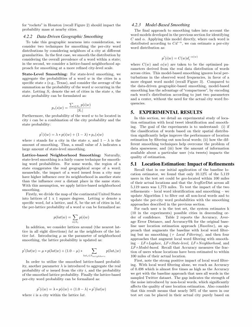
To further examine the differences among the several testedapproaches, we show in Figure 5 the error distance in milesversus the fraction of users for whom the estimator canplace within a particular error distance. The figure com-pares the original baseline user location estimation approach(Baseline), the baseline approach plus local word filtering(+ Local Filtering), and then the best performing smooth-ing approach (LF+Neighborhood) and the worst performingsmoothing approach (LF+Model-based). The x-axis iden-tifies the error distance in miles in log-scale and the y-axisquantifies the fraction of users located within a specific errordistance. We can clearly see the strong impact of local wordfiltering and the minor improvement of smoothing across all

Figure 5: Comparison Across Estimators

error distances. For the best performing approach, we cansee that nearly 30% of users are placed within 10 miles oftheir actual location in addition to the 51% within 100 miles.

5.2 Capacity of the EstimatorTo better understand the capacity of the location estima-

tor to identify the correct user location, we next relax ourrequirement that the estimator make only a single locationprediction. Instead, we are interested to see if the estimatorcan identify a good location somewhere in the top-k of itspredicted cities. Such a relaxation allows us to appreciate ifthe estimator is identifying some local signals in many cases,even if the estimator does not place the best location in thetop most probable position.

Returning to Table 2, we report the Accuracy@k for eachof the approaches. Recall Accuracy@k measures the fractionof users located within 100 miles of their actual location, forsome city in the top k predictions of the estimator. Forexample, for Accuracy@5 for LF+Neighborhood we find aresult of 0.788, meaning that within the first five estimatedlocations, we find at least one location within 100 miles ofthe actual location in 79% of cases. This indicates thatthe content-based location estimator has high capacity foraccurate location estimation, considering the top-5 cities arerecommended from a pool of all cities in the US. This is apositive sign for making further refinements and ultimatelyto improving the top-1 city prediction.

Similarly, Figure 6(a) shows the error distance distribu-tion for varying choices of k, where each point representsthe fraction of users with an error in that range (i.e., thefirst point represents errors of 0-100 miles, the second point100-200 miles, and so on). The location estimator identifiesa city in the top-10 that lies within 100 miles of a user’s

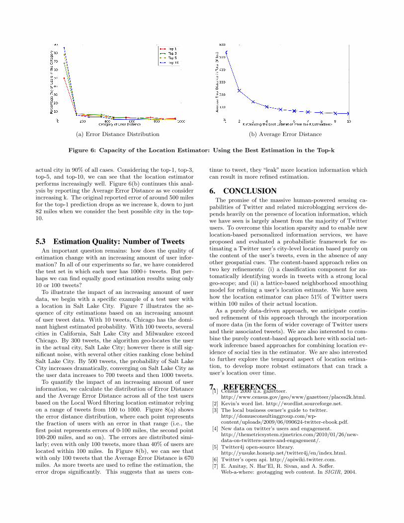
(a) Error Distance Distribution (b) Average Error Distance

Figure 6: Capacity of the Location Estimator: Using the Best Estimation in the Top-k

actual city in 90% of all cases. Considering the top-1, top-3,top-5, and top-10, we can see that the location estimatorperforms increasingly well. Figure 6(b) continues this anal-ysis by reporting the Average Error Distance as we considerincreasing k. The original reported error of around 500 milesfor the top-1 prediction drops as we increase k, down to just82 miles when we consider the best possible city in the top-10.

5.3 Estimation Quality: Number of TweetsAn important question remains: how does the quality of

estimation change with an increasing amount of user infor-mation? In all of our experiments so far, we have consideredthe test set in which each user has 1000+ tweets. But per-haps we can find equally good estimation results using only10 or 100 tweets?

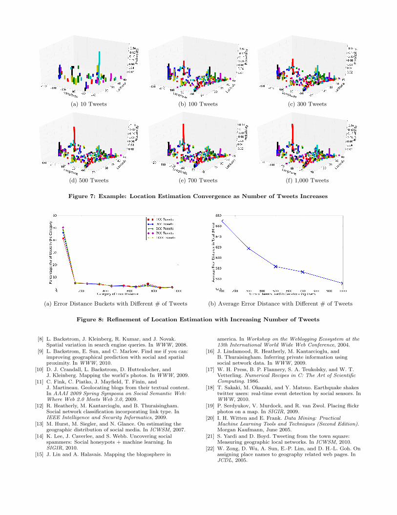
To illustrate the impact of an increasing amount of userdata, we begin with a specific example of a test user witha location in Salt Lake City. Figure 7 illustrates the se-quence of city estimations based on an increasing amountof user tweet data. With 10 tweets, Chicago has the domi-nant highest estimated probability. With 100 tweets, severalcities in California, Salt Lake City and Milwaukee exceedChicago. By 300 tweets, the algorithm geo-locates the userin the actual city, Salt Lake City; however there is still sig-nificant noise, with several other cities ranking close behindSalt Lake City. By 500 tweets, the probability of Salt LakeCity increases dramatically, converging on Salt Lake City asthe user data increases to 700 tweets and then 1000 tweets.

To quantify the impact of an increasing amount of userinformation, we calculate the distribution of Error Distanceand the Average Error Distance across all of the test usersbased on the Local Word filtering location estimator relyingon a range of tweets from 100 to 1000. Figure 8(a) showsthe error distance distribution, where each point representsthe fraction of users with an error in that range (i.e., thefirst point represents errors of 0-100 miles, the second point100-200 miles, and so on). The errors are distributed simi-larly; even with only 100 tweets, more than 40% of users arelocated within 100 miles. In Figure 8(b), we can see thatwith only 100 tweets that the Average Error Distance is 670miles. As more tweets are used to refine the estimation, theerror drops significantly. This suggests that as users con-

tinue to tweet, they “leak” more location information whichcan result in more refined estimation.

6. CONCLUSIONThe promise of the massive human-powered sensing ca-

pabilities of Twitter and related microblogging services de-pends heavily on the presence of location information, whichwe have seen is largely absent from the majority of Twitterusers. To overcome this location sparsity and to enable newlocation-based personalized information services, we haveproposed and evaluated a probabilistic framework for es-timating a Twitter user’s city-level location based purely onthe content of the user’s tweets, even in the absence of anyother geospatial cues. The content-based approach relies ontwo key refinements: (i) a classification component for au-tomatically identifying words in tweets with a strong localgeo-scope; and (ii) a lattice-based neighborhood smoothingmodel for refining a user’s location estimate. We have seenhow the location estimator can place 51% of Twitter userswithin 100 miles of their actual location.

As a purely data-driven approach, we anticipate contin-ued refinement of this approach through the incorporationof more data (in the form of wider coverage of Twitter usersand their associated tweets). We are also interested to com-bine the purely content-based approach here with social net-work inference based approaches for combining location ev-idence of social ties in the estimator. We are also interestedto further explore the temporal aspect of location estima-tion, to develop more robust estimators that can track auser’s location over time.

7. REFERENCES[1] Census 2000 u.s. gazetteer.

http://www.census.gov/geo/www/gazetteer/places2k.html.

[2] Kevin’s word list. http://wordlist.sourceforge.net.

[3] The local business owner’s guide to twitter.http://domusconsultinggroup.com/wp-content/uploads/2009/06/090624-twitter-ebook.pdf.

[4] New data on twitter’s users and engagement.http://themetricsystem.rjmetrics.com/2010/01/26/new-data-on-twitters-users-and-engagement/.

[5] Twitter4j open-source library.http://yusuke.homeip.net/twitter4j/en/index.html.

[6] Twitter’s open api. http://apiwiki.twitter.com.

[7] E. Amitay, N. Har’El, R. Sivan, and A. Soffer.Web-a-where: geotagging web content. In SIGIR, 2004.

(a) 10 Tweets (b) 100 Tweets (c) 300 Tweets

(d) 500 Tweets (e) 700 Tweets (f) 1,000 Tweets

Figure 7: Example: Location Estimation Convergence as Number of Tweets Increases

(a) Error Distance Buckets with Different # of Tweets (b) Average Error Distance with Different # of Tweets

Figure 8: Refinement of Location Estimation with Increasing Number of Tweets

[8] L. Backstrom, J. Kleinberg, R. Kumar, and J. Novak.Spatial variation in search engine queries. In WWW, 2008.

[9] L. Backstrom, E. Sun, and C. Marlow. Find me if you can:improving geographical prediction with social and spatialproximity. In WWW, 2010.

[10] D. J. Crandall, L. Backstrom, D. Huttenlocher, andJ. Kleinberg. Mapping the world’s photos. In WWW, 2009.

[11] C. Fink, C. Piatko, J. Mayfield, T. Finin, andJ. Martineau. Geolocating blogs from their textual content.In AAAI 2009 Spring Symposia on Social Semantic Web:Where Web 2.0 Meets Web 3.0, 2009.

[12] R. Heatherly, M. Kantarcioglu, and B. Thuraisingham.Social network classification incorporating link type. InIEEE Intelligence and Security Informatics, 2009.

[13] M. Hurst, M. Siegler, and N. Glance. On estimating thegeographic distribution of social media. In ICWSM, 2007.

[14] K. Lee, J. Caverlee, and S. Webb. Uncovering socialspammers: Social honeypots + machine learning. InSIGIR, 2010.

[15] J. Lin and A. Halavais. Mapping the blogosphere in

america. In Workshop on the Weblogging Ecosystem at the13th International World Wide Web Conference, 2004.

[16] J. Lindamood, R. Heatherly, M. Kantarcioglu, andB. Thuraisingham. Inferring private information usingsocial network data. In WWW, 2009.

[17] W. H. Press, B. P. Flannery, S. A. Teukolsky, and W. T.Vetterling. Numerical Recipes in C: The Art of ScientificComputing. 1986.

[18] T. Sakaki, M. Okazaki, and Y. Matsuo. Earthquake shakestwitter users: real-time event detection by social sensors. InWWW, 2010.

[19] P. Serdyukov, V. Murdock, and R. van Zwol. Placing flickrphotos on a map. In SIGIR, 2009.

[20] I. H. Witten and E. Frank. Data Mining: PracticalMachine Learning Tools and Techniques (Second Edition).Morgan Kaufmann, June 2005.

[21] S. Yardi and D. Boyd. Tweeting from the town square:Measuring geographic local networks. In ICWSM, 2010.

[22] W. Zong, D. Wu, A. Sun, E.-P. Lim, and D. H.-L. Goh. Onassigning place names to geography related web pages. InJCDL, 2005.