Vision-Based SLAM: Stereo and Monocular …mdailey/cvreadings/Lemaire-SLAM.pdf · Vision-Based SLAM: Stereo and Monocular Approaches 345 Figure 1.The ATRV rover Dala and the 10 m

International Journal of Computer Vision 74(3), 343–364, 2007

c© 2007 Springer Science + Business Media, LLC. Manufactured in the United States.

DOI: 10.1007/s11263-007-0042-3

Vision-Based SLAM: Stereo and Monocular Approaches

THOMAS LEMAIRE∗, CYRILLE BERGER, IL-KYUN JUNG AND SIMON LACROIXLAAS/CNRS 7, Ave du Colonel Roche, F-31077 Toulouse Cedex 4, France

[email protected]

Received November 18, 2005; Accepted January 23, 2007

First online version published in February, 2007

Abstract. Building a spatially consistent model is a key functionality to endow a mobile robot with autonomy. Withoutan initial map or an absolute localization means, it requires to concurrently solve the localization and mapping problems.For this purpose, vision is a powerful sensor, because it provides data from which stable features can be extracted andmatched as the robot moves. But it does not directly provide 3D information, which is a difficulty for estimatingthe geometry of the environment. This article presents two approaches to the SLAM problem using vision: one withstereovision, and one with monocular images. Both approaches rely on a robust interest point matching algorithm thatworks in very diverse environments. The stereovision based approach is a classic SLAM implementation, whereas themonocular approach introduces a new way to initialize landmarks. Both approaches are analyzed and compared withextensive experimental results, with a rover and a blimp.

Keywords: bearing only SLAM, interest point matching, 3D SLAM

1. Introduction

Autonomous navigation is a fundamental ability for mo-bile robots, be it for ground rovers, indoor robots, fly-ing or underwater robots. It requires the integration of awide variety of processes, from low-level actuator con-trol, to higher-level strategic decision making, via envi-ronment mapping and path planning. Among these var-ious functionalities, self-localization is an essential one,as it is required at various levels in the whole system,from mission supervision to fine trajectory executioncontrol:

• The missions to be achieved by the robot are oftenexpressed in localization terms, explicitly (e.g. “reachthat position” or “explore this area”) or more implicitly,such as “return to the initial position”.

• Autonomous navigation calls for the building of globalmaps of the environment, to compute trajectories orpaths and to enable mission supervision. A good esti-mate of the robot position is required to guarantee thespatial consistency of such maps.

∗Corresponding author.

• Finally, the correct execution of the geometric trajec-tories provided by the planners relies on the preciseknowledge of robot motions.

It is well known that dead reckoning techniques gen-erate position estimates with unbounded error growth, asthey compute the robot position from the composition ofelementary noisy motion estimates. Such approaches canfulfill the localization requirements for local trajectoryexecution control, but do not allow global localization.Visual motion estimation techniques from monocular se-quences (Heeger and Jepson, 1992; Vidal et al., 2001)or stereovision sequences (Zhang and Faugeras, 1992;Mallet et al., 2000; Olson et al., 2000) provide precisemotion estimates between successive data acquisitions,but they are akin to dead reckoning.

The only solution to guarantee bounded errors on theposition estimates is to rely on stable environment fea-tures. If a spatially consistent map of the environmentis available, map-based localization can be applied: anumber of successful approaches have been reported,e.g. (Borges and Aldon, 2002; Dellaert et al., 1999).1 Onthe other hand, if the robot position is perfectly known,building an environment map with the perceived data isquite trivial, the only difficulty being to deal with the

344 Lemaire et al.

uncertainty of the geometric data to fuse them in a geo-metric representation.

Simultaneous Localization and Mapping. In the ab-sence of an a priori map of the environment, the robotis facing a kind of “chicken and egg problem”: it makesobservations on the environment that are corrupted bynoise, from positions which estimates are also corruptedwith noise. These errors in the robot’s pose have an influ-ence on the estimate of the observed environment featurelocations, and similarly, the use of the observations ofpreviously perceived environment features to locate therobot provide position estimates that inherits from botherrors: the errors of the robot’s pose and the map featuresestimates are correlated.

It has been understood early in the robotic communitythat the mapping and the localization problems are inti-mately tied together (Chatila and Laumond, 1985; Smithet al., 1987), and that they must therefore be concurrentlysolved in a unified manner, turning the chicken and eggproblem into a virtuous circle. The approaches that solvethis problem are commonly denoted as “SimultaneousLocalization and Mapping”, and have now been thor-oughly studied. In particular, stochastic approaches haveproved to solve the SLAM problem in a consistent way,because they explicitly deal with sensor noise (Thrun,2002; Dissanayake et al., 2001).

Functionalities Required by SLAM. The implementa-tion of a feature-based SLAM approach encompasses thefollowing four basic functionalities:

• Environment feature selection. It consists in detect-ing in the perceived data, features of the environmentthat are salient, easily observable and whose relativeposition to the robot can be estimated. This process de-pends on the kind of environment and on the sensorsthe robot is equipped with: it is a perception process,that represents the features with a specific data struc-ture.

• Relative measures estimation. Two processes are in-volved here:

– Estimation of the feature location relatively to therobot pose from which it is observed: this is theobservation.

– Estimation of the robot motion between two featureobservations: this is the prediction. This estimatecan be provided by sensors, by a dynamic model ofrobot evolution fed with the motion control inputs,or thanks to simple assumptions, such as a constantvelocity model.

• Data association. The observations of landmarks areuseful to compute robot position estimates only if theyare perceived from different positions: they must im-

peratively be properly associated (or matched), other-wise the robot position can become totally inconsistent.

• Estimation. This is the core of the solution to SLAM:it consists in integrating the various relative measure-ments to estimate the robot and landmarks positionsin a common global reference frame. The stochasticapproaches incrementally estimate a posterior proba-bility distribution over the robot and landmarks posi-tions, with all the available relative estimates up to thecurrent time. The distribution can be written as

p(Xr (k), {X f (k)}|z, u) (1)

where Xr (k) is the current robot’s state (at time k) and{X f (k)} is the set of landmark positions, conditionedon all the feature relative observations z and controlinputs u that denote the robot motion estimates.

Besides these essential functionalities, one must alsoconsider the map management issues. To ensure the bestposition estimates as possible and to avoid high computa-tion time due to the algorithmic complexity of the estima-tion process, an active way of selecting and managing thevarious landmarks among all the detected ones is desir-able. The latter requirement has lead to various essentialcontributions on the estimation function in the literature:use of the information filter (Thrun et al., 2002), split-ting the global map into smaller sub-maps (Leonard andFeder, 2001), delayed integration of observations (Guiv-ant and Nebot, 2001) (in turn, it happens that the use ofsub-maps can help to cope with the non linearities thatcan hinder the convergence of a Kalman filter solution(Castellanos et al., 2004)).

Vision-Based SLAM. Besides obvious advantages suchas lightness, compactness and power saving that makecameras suitable to embed in any robot, vision allows thedevelopment of a wide set of essential functionalities inrobotics (obstacle detection, people tracking, visual ser-voing. . . ). When it comes to SLAM, vision also offersnumerous advantages: first, it provides data perceived ina solid angle, allowing the development of 3D SLAMapproaches in which the robot state is expressed by 6 pa-rameters. Second, visual motion estimation techniquescan provide very precise robot motion estimates. Finallyand more importantly, very stable features can be de-tected in the images, yielding the possibility to derivealgorithms that allow to match them under significantviewpoint changes: such algorithms provide robust dataassociation for SLAM.

Most SLAM approaches rely on the position estimatesof the landmarks and the robot to associate the land-marks: the landmark observations are predicted fromtheir positions and the current robot position estimate, andcompared to the current observations. When the errors on

Vision-Based SLAM: Stereo and Monocular Approaches 345

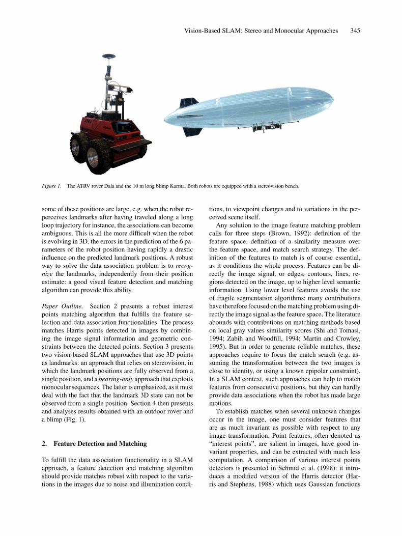
Figure 1. The ATRV rover Dala and the 10 m long blimp Karma. Both robots are equipped with a stereovision bench.

some of these positions are large, e.g. when the robot re-perceives landmarks after having traveled along a longloop trajectory for instance, the associations can becomeambiguous. This is all the more difficult when the robotis evolving in 3D, the errors in the prediction of the 6 pa-rameters of the robot position having rapidly a drasticinfluence on the predicted landmark positions. A robustway to solve the data association problem is to recog-nize the landmarks, independently from their positionestimate: a good visual feature detection and matchingalgorithm can provide this ability.

Paper Outline. Section 2 presents a robust interestpoints matching algorithm that fulfills the feature se-lection and data association functionalities. The processmatches Harris points detected in images by combin-ing the image signal information and geometric con-straints between the detected points. Section 3 presentstwo vision-based SLAM approaches that use 3D pointsas landmarks: an approach that relies on stereovision, inwhich the landmark positions are fully observed from asingle position, and a bearing-only approach that exploitsmonocular sequences. The latter is emphasized, as it mustdeal with the fact that the landmark 3D state can not beobserved from a single position. Section 4 then presentsand analyses results obtained with an outdoor rover anda blimp (Fig. 1).

2. Feature Detection and Matching

To fulfill the data association functionality in a SLAMapproach, a feature detection and matching algorithmshould provide matches robust with respect to the varia-tions in the images due to noise and illumination condi-

tions, to viewpoint changes and to variations in the per-ceived scene itself.

Any solution to the image feature matching problemcalls for three steps (Brown, 1992): definition of thefeature space, definition of a similarity measure overthe feature space, and match search strategy. The def-inition of the features to match is of course essential,as it conditions the whole process. Features can be di-rectly the image signal, or edges, contours, lines, re-gions detected on the image, up to higher level semanticinformation. Using lower level features avoids the useof fragile segmentation algorithms: many contributionshave therefore focused on the matching problem using di-rectly the image signal as the feature space. The literatureabounds with contributions on matching methods basedon local gray values similarity scores (Shi and Tomasi,1994; Zabih and Woodfill, 1994; Martin and Crowley,1995). But in order to generate reliable matches, theseapproaches require to focus the match search (e.g. as-suming the transformation between the two images isclose to identity, or using a known epipolar constraint).In a SLAM context, such approaches can help to matchfeatures from consecutive positions, but they can hardlyprovide data associations when the robot has made largemotions.

To establish matches when several unknown changesoccur in the image, one must consider features thatare as much invariant as possible with respect to anyimage transformation. Point features, often denoted as“interest points”, are salient in images, have good in-variant properties, and can be extracted with much lesscomputation. A comparison of various interest pointsdetectors is presented in Schmid et al. (1998): it intro-duces a modified version of the Harris detector (Har-ris and Stephens, 1988) which uses Gaussian functions

346 Lemaire et al.

to compute the two-dimensional image derivatives, andthat gives the best repeatability under rotation and scalechanges (the repeatability being defined as the percentageof repeated interest points between two images). How-ever the repeatability steeply decreases with significantscale changes: in such cases, a scale adaptive version ofthe Harris detector is required to allow point matching(Dufournaud et al., 2004). When no information on scalechange is available, matching features becomes quitetime consuming, scale being an additional dimensionto search through. To avoid this, scale invariant featuredetection algorithms have been proposed (Lowe, 1999).However, these methods generate much less features thanthe standard or scale adaptive detectors, especially in un-structured or highly textured environments, and requiremore computing time.

2.1. Interest Points

To locate points in the image where the signal changesbi-directionally, the Harris corner detector computes thelocal moment matrix M of two normal gradients of in-tensity for each pixel x = (u, v) in the image (Harris andStephens, 1988):

M(x, σ ) = G(x, σ ) ⊗(

Iu(x)2 Iu(x)Iv(x)Iu(x)Iv(x) Iv(x)2

)(2)

where G(., σ ) is the Gaussian kernel of standard devia-tion σ , and Iu(.) and Iv(.) are the first order derivatives ofthe intensity respectively in the u and v directions. Theeigenvalues (λ1, λ2) of M(x, σ ) are the principal curva-tures of the auto-correlation function: the pixels for whichthey are locally maximum are declared as interest points.It has been shown in Schmid et al. (1998) that interestpoints are more stable when the derivatives are computedby convolving the image with Gaussian derivatives:

Iu(x, σ ) = Gu(x, σ ) ⊗ I (x)

Iv(x, σ ) = Gv(x, σ ) ⊗ I (x)

where Gu(., σ ), Gv(., σ ) are the first order derivatives ofthe Gaussian kernel of standard deviation σ along theu and v directions. The auto-correlation matrix is thendenoted M(x, σ, σ ). Note that to maintain the deriva-tives stable with respect to the image scale change s,the Gaussian functions can be normalized with respectto s—the auto-correlation matrix is then M(x, σ, σ , s)(Dufournaud et al., 2004).

Point Similarity. If the geometric transformation T be-tween two images I and I ′ is strictly equal to a scalechange s and rotation change θ , the following equality is

satisfied for two matching points (x, x′) in the images:(Iu(x, σ, θ )Iv(x, σ, θ)

)= R(θ )

(Iu(x, σ )Iv(x, σ )

)=

(I ′u′ (x′, sσ )

I ′v′ (x′, sσ )

)where R(θ ) is the rotation and Iu(x, σ, θ) and Iv(x, σ, θ)are the steered Gaussian derivatives of the image in thedirection θ (Freeman and Adelson, 1991). As a conse-quence, we can write:

R(θ )M(x, σ, σ )R(θ )T = M(x′, σ, σ , s)

Since

M(x, σ, σ ) = U

(λ1 00 λ2

)U T

and

M(x′, σ, σ , s) = U ′(

λ′1 0

0 λ′2

)U ′T

where the columns of U and U ′ are the eigenvectors.The principal curvatures of the two matched points aretherefore equal: λ1 = λ′

1 and λ2 = λ′2.

For two matching points in two images of real 3Dscenes, this equality is of course not strictly verified, be-cause of signal noise, and especially because the truetransformation of the image is seldom strictly equal to arotation and scale change. We define the point similar-ity Sp between two interest points on the basis of theireigenvalues and their intensity:

SP (x, x′) = Sp1(x, x′) + Sp2(x, x′) + SpI (x, x′)3

where

Sp1(x, x′) = min(λ1, λ′1)

max(λ1, λ′1)

,

Sp2(x, x′) = min(λ2, λ′2)

max(λ2, λ′2)

,

and SpI (x, x′) = min(I (x), I ′(x′))max(I (x), I ′(x′))

The maximum similarity is 1.0. Statistics show thatthe evolution of Sp1 and Sp2 for matched points is hardlyaffected by rotation and scale changes, and is alwayslarger than 0.8 (Fig. 2).

2.2. Matching Interest Points

To match interest points, a cross-correlation measure ofthe signal can be used (Lhuillier and Quan, 2003), butthis requires a precise knowledge of the search area. Tocope with this, local grayvalue invariants can be used,


100

90

80

70

60

Ratio (

%)

50

40

30

20

10

00 20 40 60 80 100

Rotation change (degree)

120 140 160 180 1.1 1.15 1.2 1.25 1.3 1.35

Rotation change (degree)

1.4 1.45 1.5 1.55 1.6

with s = 1.5

with s = 1.0

100

90

80

70

60

Ratio (

%)

50

40

30

20

10

0

Repeatability

Sigma(Sp2)

Sigma(Sp1)

Point similarity2 (Sp2)


Repeatability

Sigma(Sp2)

Sigma(Sp1)



Figure 2. Evolution of the mean and standard deviation of matching points similarity with known rotation (left) and scale changes (right). On the

right curve, the solid lines represent the evolution of the similarity when the scale of the detector is set to 1: the similarity decreases when the scale

change between the images increases. The dashed lines show the values of the similarity when the scale of the detector is set to 1.5: the similarity is

then closer to one when the actual scale change between the images is of the same order.

as in Schmid and Mohr (1997). The approach we pro-pose here imposes a combination of geometric and sig-nal similarity constraints, thus being more robust thanapproaches solely based on point signal characteristics(a simpler version of this algorithm has been presentedin Jung and Lacroix (2001)). It relies on interest pointgroup matching: an interest point group is a small set ofneighbor interest points, that represent a small region ofthe image. With groups composed of a small number ofinterest points, the corresponding region is small enoughto ensure that a simple rotation θ approximates fairly wellthe actual region transformation between the images—the translation being ignored here. The estimate of thisrotation is essential in the algorithm, as a group match hy-pothesis (i.e. a small set of point matches) is assessed onboth the signal similarity between interest points and thepoint matches compliance with the rotation. The match-ing procedure is a seed-and-grow algorithm initiated bya reliable group match (see Algorithm 1).

Algorithm 1 Overview of the interest point matchingalgorithmGiven two images I and I ′:

1. Extract the interest points {x} and {x′} in both im-ages

2. In both images, establish the groups of extractedpoints. This defines two sets of groups G = {G}and G′ = {G ′}, and the neighborhood relations es-tablish a graph between the detected points—thisprocedure is depicted in Section 2.2.1.

3. While G �= ∅:

(a) Establish an initial group match M(Gi ,G ′j ),

which defines a rotation θi, j , and remove Gi

from G—this procedure is depicted in Section2.2.2.

(b) Recursive propagation: starting from theneighbors ofGi , explore the neighboring pointsto find group matches compliant with θi, j . Re-move the new matched groups from G, and it-erate until no matches compliant with θi, j canbe found—this procedure is depicted in Sec-tion 2.2.3.

4. Check the validity of the propagated group matches

2.2.1. Grouping Process. The sets of interest points{x}, {x′} detected respectively in the two images I, I ′ arestructured in local groups, formed by a pivot point g0 andits n closest neighbors {g1, . . . , gn} (Fig. 3). To ensurethat the image region covered by the points of a groupis small enough, n is rather small (e.g. we use n = 5).The groups are generated by studying the neighborhood

Figure 3. Illustration of the point grouping procedure, with n = 2 for

readability purposes. Groups have not been generated around points aand b as they are too close to the image border, and neither around d as

no neighbor is close enough. Three groups have been generated, with

points c, e and f as a pivot. b → e means “b is a neighbor of e”, which

defines a graph relation between the points.

348 Lemaire et al.

of each point following a spiral pattern: the groupingprocess is stopped if the spiral meets the image borderbefore n neighbors are found. Also, a maximum thresholdon the distance between the neighbor points and the pivotis applied, to avoid the formation of groups that cover atoo large image region (in low textured areas for instance,where there are scarce interest points). This implies thata few points do not belong to any group: their matchingis processed individually (see Section 2.2.3).

After the grouping process, we end up with two groupsets G = {G1, . . . ,GN } and G′ = {G ′

1, . . . ,G ′M}, Gi de-

noting the local group generated with the point xi as apivot:

Gi = {g0, g1, . . . , gn}, g0 = xi

The neighbors {g1, . . . , gn} are ordered by their dis-tance to the pivot:

‖v1 ‖< · · · <‖vn ‖

where the vectors vi are defined as vi = gi −g0 and ‖ . ‖is the norm operator. For each neighbor of the group, wealso compute its angle, defined as:

θgp = tan−1(vp · v, vp · u)

where u and v are the image axes.

2.2.2. Group Matching. The procedure to establish agroup match is essential in our approach: in particular, awrong initial group match would cause the algorithm tofail. The procedure consists in three steps depicted in thenext paragraphs:

1. Given a group Gi in I with g0 as a pivot, all the groupsG ′

j in I ′ whose pivot g′0 is similar to g0 are candidate

group matches.2. For each candidate group match G ′

j , determine all thegroup match hypotheses H (Gi ,G ′

j ) on the basis of thepossible individual neighbor matches, and select thebest one H∗(Gi ,G ′

j ).3. Select the best group match among all the H∗(Gi ,G ′

j ),and apply a validation criteria.

Point Similarity. Two points x, x′ are defined as similarif their similarity measure is above a threshold TSp :

SP (x, x′) > TSP

This test is used to asses the similarity of points insteps 1 and 2 of the group matching procedure.

Building Group Match Hypotheses. Given two groups(Gi ,G ′

j ) whose pivots have passed the point similar-ity test, one must evaluate all the possible associated

group match hypotheses, i.e. the various combinationsof matches between the neighbor points of the groups. Agroup match hypothesis H (Gi ,G ′

j ) is defined as:

• a rotation θ

• a set M(Gi ,G ′j ) of interest point matches which respect

the rotation θ and whose similarity score is above thethreshold TSP :

M(Gi ,G ′j ) = {(gp, g′

q ) ∈ Gi × G ′j | SP (gp, g′

q ) > TSP

and |θgp − θg′q| < Tθ } ∪ {(g0, g′

0)}

• a group hypothesis similarity score SG , defined as thesum of the similarity of the corresponding matchedinterest points:

SG(H (Gi ,G ′j )) =

∑(gp,g′

q )∈M(Gi ,G ′j )

SP (gp, g′q )

The best group match hypothesis among all the onesthat can be defined on the basis of two candidate groups(Gi ,G ′

j ) is determined according to Algorithm 2: this pro-vides the best group match hypothesis H∗, if it exists, be-tween Gi and G ′

j . Note in this procedure the introductionof a threshold �SG in the comparison of hypotheses, toensure that the best hypotheses has a much better scorethan the second best: this is useful to avoid wrong groupmatches for images with repetitive patterns, in whichmany points are similar.

Algorithm 2 Determination of the best match hypothesisfor two groups

• Init: S∗G = 0

• For p = 1 to |Gi |, For q = 1 to |G ′j |:

• if SP (gp, g′q ) > TSP then create and evaluate a

group match hypothesis Hp,q (Gi ,G ′j ):

– Set M(Gi ,G ′j ) = {(g0, g′

0), (gp, g′q )}. This de-

fines the rotation θ for this hypothesis: θ =θgp − θg′

q

– complete M(Gi ,G ′j ) with the other points in Gi

that are similar to points in G ′j , such that:

∀s > p and t > q, SP (gs, g′t ) < TSP

and |θ − (θgs − θg′t)| < Tθ

Note here that the fact that the neighbor are or-dered by their distance to the pivot reduces thesearch for additional point matches—see Fig. 4.

– Evaluate the hypothesis Hp,q (Gi ,G ′j ):

if SG(Hp,q (Gi ,G ′j )) > S∗

G + �SG ,

then H∗ = Hp,q (Gi ,G ′j ) andS∗

G = SG(H∗).


Figure 4. Completion of a group match hypothesis. Given the hypothesis H4,3 defined by the point matches (g0, g′0) and (g4, g′

3), the best potential

match for g5 is determined by evaluating geometric and point similarity constraints. The indexes of the neighbors being ordered according to their

distance to the pivot, only the matches (g5, g′4), and (g5, g′

5) are evaluated—on this example, (g5, g′5) is the sole valid match.

Selection of the Best Group Match Hypothesis. Nowthat we have determined the best group match hypothesisH∗ for each candidate group match G ′

j for the group Gi ,one must determine the one that actually corresponds toa true group match. This is simply done by comparingtheir similarity SG , applying the same threshold �SG asabove to make sure the best match is not ambiguous.

Finally, the validity of the found group match is con-firmed by evaluating the zero-mean normalized corre-lation score (ZNCC) between windows centered on thepivots (g0, g′

0) of the groups. This score can be computedthanks to the knowledge of the rotation θ defined by thegroup match hypothesis, which is applied to the pixels ofthe window centered on g′

0.

2.2.3. Finding Further Matches

Propagation Process. Once a reliable group match hy-pothesis is established, a propagation process searchesfor new matches. The principle of the propagation is toexploit the graph defined by the grouping process andthe estimated rotation associated to the current hypoth-esis: additional point matches consistent with the cur-rent rotation estimate are searched in the neighborhoodof the current group match. This process is depicted inAlgorithm 3 .

Algorithm 3 Propagation process

Given a group match (Gi ,G ′j ) and the associated rotation

θ :

• Init: set M propage = M(Gi ,G ′j ) \ {(g0, g′

0)}.• While M propage �= ∅:

– Select a point match (gp, g′q ) ∈ M propage. gp

and g′q are respectively the pivots of the groups

Gp and G ′q .

– For s = 1 to |Gp|, For t = 1 to |G ′q |:

if SP (gs, g′t ) < TSP and |θ − (θgs − θg′

t)| < Tθ ,

add (gs, g′t ) to M propage

– Remove (gp, g′q ) from M propage

During the propagation, the translation betweenmatched points is computed: when the propagation ends,this allow to focus the search for new matches, as illus-trated in Fig. 5.

Propagation Monitoring. Repetitive patterns with asize similar to the group size can lead to false matches,although the initial group match has passed the tests de-scribed in Section 2.2.2. The occurrence of such cases canbe detected by checking whether the propagation processsucceeds or not around the first group match: if it fails,it is very likely that the initial group match hypothesis isa wrong one, and it is then discarded (Fig. 6). Note thatthis test also eliminates group matches if a group is iso-lated or if the overlap between the two images I and I ′ isrestricted to the size of the group: these are degeneratedcases in which the algorithm does not match the groups.

Non-Grouped Points Matching. As mentioned inSection 2.2.1, some points are not associated to groupsafter the grouping procedure, mainly near the image bor-ders. Once the propagation procedure is achieved, foreach non grouped point xb of I, matches are searchedamong the set of points Xb in the image I ′:

Xc = {x|x ∈ W (x′b)}

where x′b is the estimated position of xb in I ′ provided

by the application of the transformation defined by themean of the rotations and translations estimated so far,and W (x′

b) is a search window centered on x′b. The points

350 Lemaire et al.

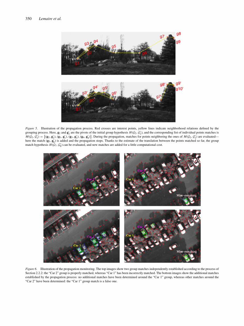
Figure 5. Illustration of the propagation process. Red crosses are interest points, yellow lines indicate neighborhood relations defined by the

grouping process. Here, g2 and g′2 are the pivots of the initial group hypothesis H (G2,G′

2), and the corresponding list of individual points matches is

M(G2,G′2) = {

(g2, g′2), (g1, g′

1), (g3, g′3), (g4, g′

4)}. During the propagation, matches for points neighboring the ones of M(G2,G′

2) are evaluated—

here the match (g5, g′6) is added and the propagation stops. Thanks to the estimate of the translation between the points matched so far, the group

match hypothesis H (G7,G′8) can be evaluated, and new matches are added for a little computational cost.

Figure 6. Illustration of the propagation monitoring. The top images show two group matches independently established according to the process of

Section 2.2.2: the “Car 2” group is properly matched, whereas “Car 1” has been incorrectly matched. The bottom images show the additional matches

established by the propagation process: no additional matches have been determined around the “Car 1” group, whereas other matches around the

“Car 2” have been determined: the “Car 1” group match is a false one.


Figure 7. Points matched with a small viewpoint change and significant scene modifications (throughout the paper, red crosses shows the interest

points, and green squares indicate successful matches). 349 matches are found in 200 ms (115 ms for the points detection, 85 ms for the matching

process.

Figure 8. Points matched with a significant viewpoint change, that induces a 1.5 scale change. 57 points are matched in 80 ms.

comprised in W (x′b) are evaluated according to the hy-

pothesis pruning process presented in Section 2.2.2: teston the point similarity measure SP and verification withthe computation of the ZNCC coefficient.

2.3. Results

The algorithm provides numerous good matches whilekeeping the number of outliers very small, in differ-ent kinds of scenes and in a wide variety of conditions,tolerating noticeable scene modifications and viewpointchanges. Figures 7 to 9 present matches obtained in var-ious conditions, with the computational time required—the processed image size is 512 × 384, and time mea-sures have been obtained on 3.2 GHz Pentium IV). Thealgorithm does not explore various scale changes: whena scale change greater than half a unity occurs, it mustbe provided as a parameter to the interest point detec-tion routine. This is a limitation as compared to scaleinvariant point features, but a coarse knowledge of the

scale change is sufficient: in a SLAM context, such anestimate is readily obtained.

Table 1 lists the parameters required by the matchingalgorithm and their values. These values are used for allthe results presented throughout the paper, and duringour everyday use of the algorithm: no parameter tuningis required.

Three parameters are used during the grouping pro-cess presented Section 2.2.1: Minimum group size, Max-imum group size and Maximum distance between pivotand group member (the size parameters do not include

Table 1. Thresholds and parameters of the matching algorithm.

Maximum group size 5

Minimum group size 2

Size of correlation window for ZNCC 9 × 9

Threshold TSP on point similarity SP 0.7

Threshold on ZNCC TZNCC 0.6

Threshold �SG to discriminate group hypotheses 0.1

Threshold on rotation change, Tθ 0.2rad

352 Lemaire et al.

Figure 9. Points matched with a scale change of 3. 70 points are matched in 270 ms.

the pivot). The Minimum group size is naturally set to 2,the minimum size that allows to run the group matchesdetermination presented Section 2.2.2. The Maximumgroup size is a compromise: on the one hand, the moremembers in a group, the more reliable are the group matchhypotheses. On the other hand, a big number of points ina group tends to violate the hypothesis that a simple ro-tation approximates its transformation between the twoimages: empirical tests show that a value of 5 offers agood balance. Finally, the Maximum distance betweenpivot and group member threshold is set to 3

√D, where

D is the density of interest points in the image.The threshold TSP on the similarity measure is used to

evaluate if two points match: its value is set to 0.7, accord-ing to the variations of the point similarities presentedin Section 2.1. The threshold TZNCC on the correlationscore to confirm a point match is set to 0.6, a valuesmaller than usually used for this score (e.g. in densestereovision): this is due to the fact that a rotation is im-posed to one of the correlation window before comput-ing the score, which smooths the signal in the window,and also to the fact that we aim at matching points seenfrom different viewpoints. Finally, the threshold on ro-tation change Tθ is set to 0.2rad, a quite large valuethat is necessary to cope with the errors on the inter-est points detection, that can reach at most 1.5 pixel(Schmid et al., 1998).

3. Vision-Based SLAM

The vision algorithms of Section 2 provide a solution fortwo of the four basic SLAM functionalities introduced inSection 1: the observed features are the interest points,and data association is performed by the interest pointmatching process.

There are however two important cases to distin-guish regarding the observation function, depending

on whether the robot is endowed with stereovision ornot:

• With stereovision, the 3D coordinates of the featureswith respect to the robot are simply provided by match-ing points in the stereoscopic image pair,

• But if the robot is endowed with a single camera, onlythe bearings of the features are observed: this requiresa dedicated landmark initialization procedure, that in-tegrates several observations over time.

This section presents how we set up a SLAM solutionin both cases, focusing on the monocular case, whichraises specific difficulties. Note that regarding the over-all SLAM estimation process, vision does not raise anyparticular problem—we use a classical implementationof the Extended Kalman Filter in our developments.

3.1. SLAM with Stereovision

A vast majority of existing SLAM approaches rely ondata that directly convey the landmark 3D state (e.g. us-ing laser range finders or millimeter wave radars). Stere-ovision falls in this category, but it is only recently thatthis sensor has been used to develop SLAM approaches.In Se et al. (2002), an approach that uses scale invari-ant features (SIFT) is depicted, with results obtained bya robot evolving in 2D in a 10 × 10 m2 laboratory en-vironment, in which about 3500 landmarks are mappedin 3D. In Kim and Sukkarieh (2003), rectangular patchesare spread on a horizontal ground and used as landmarks.This is not strictly speaking a stereovision approach, butthe distance to the landmarks is readily observable as thelandmarks have a known size. Our first contribution to thisproblem has been published in Jung and Lacroix (2003),with some preliminary results obtained on a stereovisionbench mounted on a blimp.


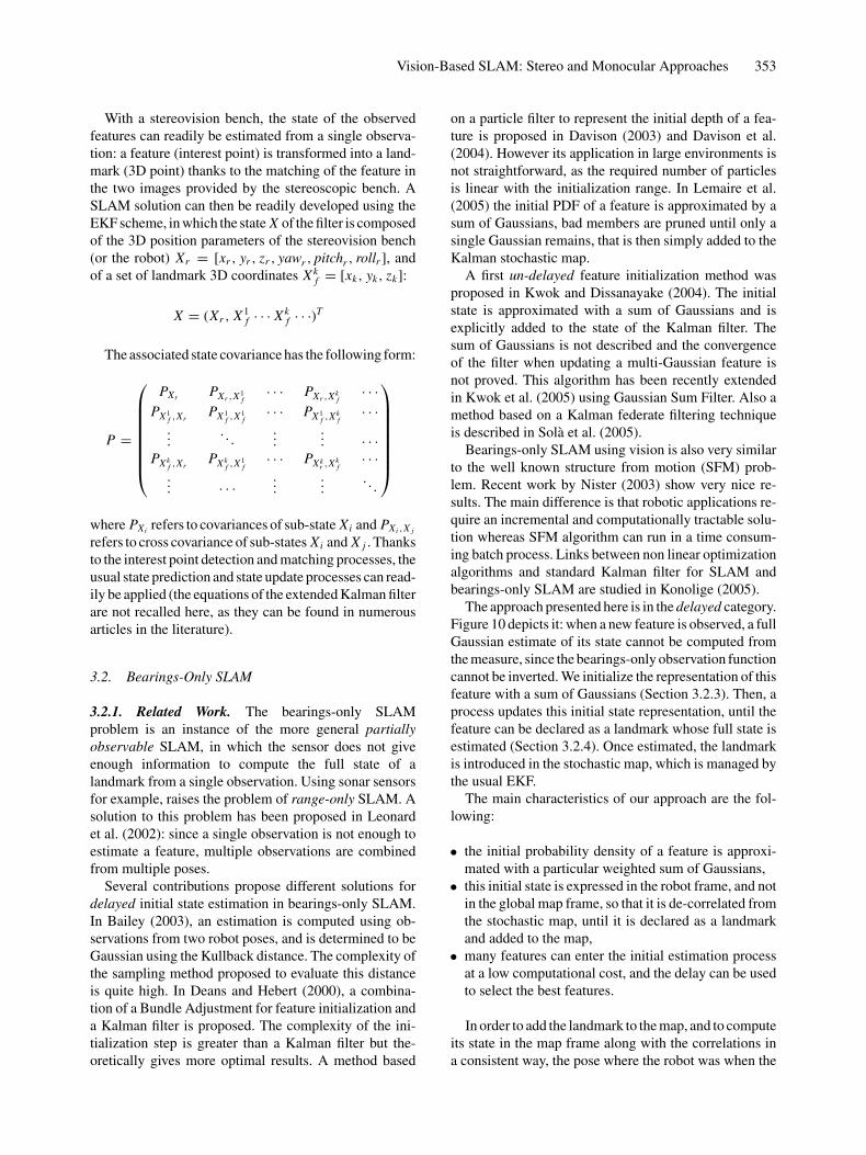
With a stereovision bench, the state of the observedfeatures can readily be estimated from a single observa-tion: a feature (interest point) is transformed into a land-mark (3D point) thanks to the matching of the feature inthe two images provided by the stereoscopic bench. ASLAM solution can then be readily developed using theEKF scheme, in which the state X of the filter is composedof the 3D position parameters of the stereovision bench(or the robot) Xr = [xr , yr , zr , yawr , pitchr , rollr ], andof a set of landmark 3D coordinates Xk

f = [xk, yk, zk]:

X = (Xr , X1f · · · Xk

f · · ·)T

The associated state covariance has the following form:

P =

⎛⎜⎜⎜⎜⎜⎜⎜⎝

PXr PXr ,X1f

· · · PXr ,Xkf

· · ·PX1

f ,XrPX1

f ,X1f

· · · PX1f ,Xk

f· · ·

.... . .

...... · · ·

PXkf ,Xr

PXkf ,X1

f· · · PXk

r ,Xkf

· · ·... · · · ...

.... . .

⎞⎟⎟⎟⎟⎟⎟⎟⎠where PXi refers to covariances of sub-state Xi and PXi ,X j

refers to cross covariance of sub-states Xi and X j . Thanksto the interest point detection and matching processes, theusual state prediction and state update processes can read-ily be applied (the equations of the extended Kalman filterare not recalled here, as they can be found in numerousarticles in the literature).

3.2. Bearings-Only SLAM

3.2.1. Related Work. The bearings-only SLAMproblem is an instance of the more general partiallyobservable SLAM, in which the sensor does not giveenough information to compute the full state of alandmark from a single observation. Using sonar sensorsfor example, raises the problem of range-only SLAM. Asolution to this problem has been proposed in Leonardet al. (2002): since a single observation is not enough toestimate a feature, multiple observations are combinedfrom multiple poses.

Several contributions propose different solutions fordelayed initial state estimation in bearings-only SLAM.In Bailey (2003), an estimation is computed using ob-servations from two robot poses, and is determined to beGaussian using the Kullback distance. The complexity ofthe sampling method proposed to evaluate this distanceis quite high. In Deans and Hebert (2000), a combina-tion of a Bundle Adjustment for feature initialization anda Kalman filter is proposed. The complexity of the ini-tialization step is greater than a Kalman filter but the-oretically gives more optimal results. A method based

on a particle filter to represent the initial depth of a fea-ture is proposed in Davison (2003) and Davison et al.(2004). However its application in large environments isnot straightforward, as the required number of particlesis linear with the initialization range. In Lemaire et al.(2005) the initial PDF of a feature is approximated by asum of Gaussians, bad members are pruned until only asingle Gaussian remains, that is then simply added to theKalman stochastic map.

A first un-delayed feature initialization method wasproposed in Kwok and Dissanayake (2004). The initialstate is approximated with a sum of Gaussians and isexplicitly added to the state of the Kalman filter. Thesum of Gaussians is not described and the convergenceof the filter when updating a multi-Gaussian feature isnot proved. This algorithm has been recently extendedin Kwok et al. (2005) using Gaussian Sum Filter. Also amethod based on a Kalman federate filtering techniqueis described in Sola et al. (2005).

Bearings-only SLAM using vision is also very similarto the well known structure from motion (SFM) prob-lem. Recent work by Nister (2003) show very nice re-sults. The main difference is that robotic applications re-quire an incremental and computationally tractable solu-tion whereas SFM algorithm can run in a time consum-ing batch process. Links between non linear optimizationalgorithms and standard Kalman filter for SLAM andbearings-only SLAM are studied in Konolige (2005).

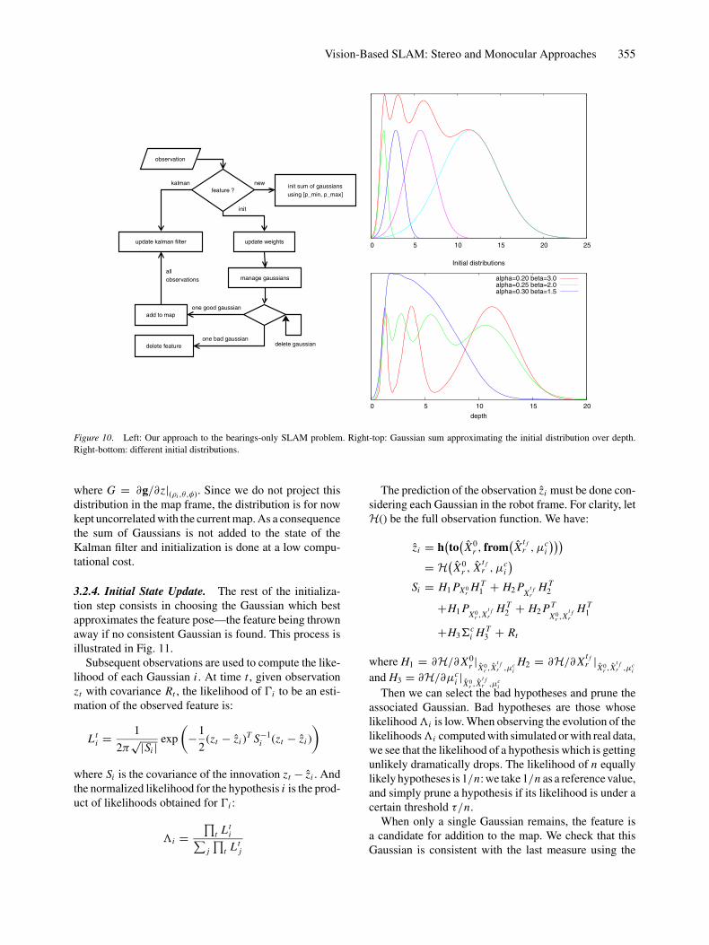
The approach presented here is in the delayed category.Figure 10 depicts it: when a new feature is observed, a fullGaussian estimate of its state cannot be computed fromthe measure, since the bearings-only observation functioncannot be inverted. We initialize the representation of thisfeature with a sum of Gaussians (Section 3.2.3). Then, aprocess updates this initial state representation, until thefeature can be declared as a landmark whose full state isestimated (Section 3.2.4). Once estimated, the landmarkis introduced in the stochastic map, which is managed bythe usual EKF.

The main characteristics of our approach are the fol-lowing:

• the initial probability density of a feature is approxi-mated with a particular weighted sum of Gaussians,

• this initial state is expressed in the robot frame, and notin the global map frame, so that it is de-correlated fromthe stochastic map, until it is declared as a landmarkand added to the map,

• many features can enter the initial estimation processat a low computational cost, and the delay can be usedto select the best features.

In order to add the landmark to the map, and to computeits state in the map frame along with the correlations ina consistent way, the pose where the robot was when the

354 Lemaire et al.

feature was first seen has to be estimated in the filter. Allobservations of the feature are also memorized along thecorresponding robot pose estimations, so that all availableinformation is added to the filter at initialization.

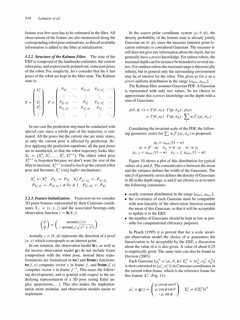
3.2.2. Structure of the Kalman Filter. The state of theEKF is composed of the landmarks estimates, the currentrobot pose, and as previously pointed out, some past posesof the robot. For simplicity, let’s consider that the k lastposes of the robot are kept in the filter state. The Kalmanstate is:

X =

⎛⎜⎜⎜⎜⎜⎜⎜⎝

X 0r

...Xk

r

X 0f

...

⎞⎟⎟⎟⎟⎟⎟⎟⎠P =

⎛⎜⎜⎜⎜⎜⎜⎜⎜⎝

PX0r

· · · PX0r ,Xk

rPX0

r ,X0f

· · ·...

. . ....

... · · ·PXk

r ,X0r

· · · PXkr

PXkr ,X0

f· · ·

PX0f ,X0

r· · · PX0

f ,Xkr

PX0f

· · ·... · · ·

......

. . .

⎞⎟⎟⎟⎟⎟⎟⎟⎟⎠In our case the prediction step must be conducted with

special care since a whole part of the trajectory is esti-mated. All the poses but the current one are static states,so only the current pose is affected by prediction. Be-fore applying the prediction equations, all the past posesare re-numbered, so that the robot trajectory looks like:Xr = [X0

r , X2r , . . . , Xk

r , Xk+1r ]. The oldest robot pose

Xk+1r is forgotten because we don’t want the size of the

filter to increase. Xk+1r is used to back up the current robot

pose and becomes X1r (ring buffer mechanism):

X1r ← X0

r PX1r← PX0

r∀ j PX1

r ,X jf← PX0

r ,X jf

PX1r ,Xi

r← PX0

r ,Xir

i �= 0 i �= 1 PX1r ,X0

r← PX0

r

3.2.3. Feature Initialization. From now on we consider3D point features represented by their Cartesian coordi-nates X f = (x, y, z) and the associated bearings-onlyobservation function z = h(X f ):(

θ

φ

)=

(arctan(y/x)

− arctan(z/√

x2 + y2)

)Actually z = (θ, φ) represents the direction of a pixel

(u, v) which corresponds to an interest point.In our notation, the observation model h(), as well as

the inverse observation model g() do not include framecomposition with the robot pose, instead these trans-formations are formalized in to() and from() functions:to( f, v) computes vector v in frame f , and from( f, v)computes vector v in frame f −1. This eases the follow-ing developments, and is general with respect to the un-derlying representation of a 3D pose (using Euler an-gles, quaternions,. . . ). This also makes the implemen-tation more modular, and observation models easier toimplement.

In the sensor polar coordinate system (ρ, θ, φ), thedensity probability of the feature state is already jointlyGaussian on (θ, φ), since the measure (interest point lo-cation estimate) is considered Gaussian. The measure it-self does not give any information about the depth, but wegenerally have a priori knowledge. For indoor robots, themaximal depth can for instance be bounded to several me-ters. For outdoor robots the maximal range is theoreticallyinfinity, but in general only the surrounding environmentmay be of interest for the robot. This gives us for ρ an apriori uniform distribution in the range [ρmin, ρmax ].

The Kalman filter assumes Gaussian PDF. A Gaussianis represented with only two values. So we choose toapproximate this a priori knowledge on the depth with asum of Gaussians:

p(θ, φ, s) = �(θ, σθ ) · �(φ, σφ) · p(ρ)

= �(θ, σθ ) · �(φ, σφ) ·∑

i

wi�i (ρi , σρi )

Considering the invariant scale of the PDF, the follow-ing geometric series for

∑i wi�i (ρi , σρi ) is proposed:

ρ0 = ρmin/(1 − α)ρi = β i · ρ0 σρi = α · ρi wi ∝ ρi

ρn−2 < ρmax/(1 − α) ρn−1 ≥ ρmax/(1 − α)

Figure 10 shows a plot of this distribution for typicalvalues of α and β. The constant ratio α between the meanand the variance defines the width of the Gaussians. Therate β of geometric series defines the density of Gaussiansto fill in the depth range. α and β are chosen so as to meetthe following constraints:

• nearly constant distribution in the range [ρmin, ρmax ],• the covariance of each Gaussian must be compatible

with non-linearity of the observation function aroundthe mean of this Gaussian, so that it will be acceptableto update it in the EKF,

• the number of Gaussians should be kept as low as pos-sible for computational efficiency purposes.

In Peach (1995) it is proved that for a scale invari-ant observation model the choice of α guarantees thelinearization to be acceptable by the EKF, a discussionabout the value of α is also given. A value of about 0.25is empirically good. The same ratio can also be found inDavison (2003).

Each Gaussian {μpi = (ρi , θ, φ), �

pi = (σ 2

ρi, σ 2

θ , σ 2φ )}

is then converted to {μci , σ

ci )} in Cartesian coordinates in

the current robot frame, which is the reference frame forthis feature X

t fr (Fig. 11):

μci = g(z) =

⎛⎝ρi cos φ cos θ

ρi cos φ sin θ

−ρi sin φ

⎞⎠ �ci = G�

pi GT


observation

feature ?init sum of gaussians

using [p_min, p_max]

update weightsupdate kalman filter

new

init

kalman

manage gaussians

add to map

all

observations

one good gaussian

delete gaussiandelete feature

one bad gaussian

0 5 10 15 20 25

0 5 10 15 20

depth

Initial distributions

alpha=0.20 beta=3.0alpha=0.25 beta=2.0alpha=0.30 beta=1.5

Figure 10. Left: Our approach to the bearings-only SLAM problem. Right-top: Gaussian sum approximating the initial distribution over depth.

Right-bottom: different initial distributions.

where G = ∂g/∂z|(ρi ,θ,φ). Since we do not project thisdistribution in the map frame, the distribution is for nowkept uncorrelated with the current map. As a consequencethe sum of Gaussians is not added to the state of theKalman filter and initialization is done at a low compu-tational cost.

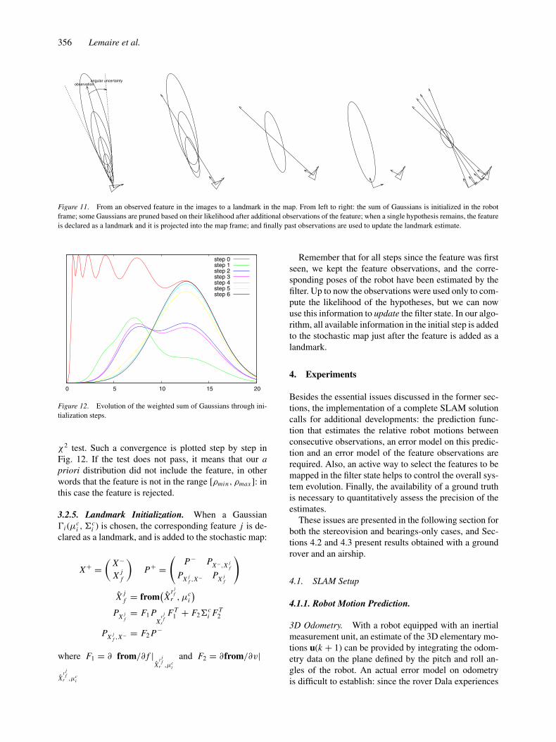
3.2.4. Initial State Update. The rest of the initializa-tion step consists in choosing the Gaussian which bestapproximates the feature pose—the feature being thrownaway if no consistent Gaussian is found. This process isillustrated in Fig. 11.

Subsequent observations are used to compute the like-lihood of each Gaussian i . At time t , given observationzt with covariance Rt , the likelihood of �i to be an esti-mation of the observed feature is:

Lti = 1

2π√|Si |

exp

(−1

2(zt − zi )

T S−1i (zt − zi )

)where Si is the covariance of the innovation zt − zi . Andthe normalized likelihood for the hypothesis i is the prod-uct of likelihoods obtained for �i :

�i =∏

t Lti∑

j

∏t Lt

j

The prediction of the observation zi must be done con-sidering each Gaussian in the robot frame. For clarity, letH() be the full observation function. We have:

zi = h(to

(X0

r , from(X

t fr , μc

i

)))= H

(X0

r , Xt fr , μc

i

)Si = H1 PX0

rH T

1 + H2 PX

t fr

H T2

+H1 PX0

r ,Xt fr

H T2 + H2 PT

X0r ,X

t fr

H T1

+H3�ci H T

3 + Rt

where H1 = ∂H/∂ X0r |X0

r ,Xt fr ,μc

iH2 = ∂H/∂ X

t fr |

X0r ,X

t fr ,μc

i

and H3 = ∂H/∂μci |X0

r ,Xt fr ,μc

iThen we can select the bad hypotheses and prune the

associated Gaussian. Bad hypotheses are those whoselikelihood �i is low. When observing the evolution of thelikelihoods �i computed with simulated or with real data,we see that the likelihood of a hypothesis which is gettingunlikely dramatically drops. The likelihood of n equallylikely hypotheses is 1/n: we take 1/n as a reference value,and simply prune a hypothesis if its likelihood is under acertain threshold τ/n.

When only a single Gaussian remains, the feature isa candidate for addition to the map. We check that thisGaussian is consistent with the last measure using the

356 Lemaire et al.

angular uncertaintyobservation

Figure 11. From an observed feature in the images to a landmark in the map. From left to right: the sum of Gaussians is initialized in the robot

frame; some Gaussians are pruned based on their likelihood after additional observations of the feature; when a single hypothesis remains, the feature

is declared as a landmark and it is projected into the map frame; and finally past observations are used to update the landmark estimate.

0 5 10 15 20

step 0step 1step 2step 3step 4step 5step 6

Figure 12. Evolution of the weighted sum of Gaussians through ini-

tialization steps.

χ2 test. Such a convergence is plotted step by step inFig. 12. If the test does not pass, it means that our apriori distribution did not include the feature, in otherwords that the feature is not in the range [ρmin, ρmax ]: inthis case the feature is rejected.

3.2.5. Landmark Initialization. When a Gaussian�i (μ

ci , �

ci ) is chosen, the corresponding feature j is de-

clared as a landmark, and is added to the stochastic map:

X+ =(

X−

X jf

)P+ =

(P− PX−,X j

f

PX jf ,X− PX j

f

)X j

f = from(X

t jf

r , μci

)PX j

f= F1 P

Xt

jf

r

F T1 + F2�

ci F T

2

PX jf ,X− = F2 P−

where F1 = ∂ from/∂ f |X

tjf

r ,μci

and F2 = ∂from/∂v|

Xt

jf

r ,μci

Remember that for all steps since the feature was firstseen, we kept the feature observations, and the corre-sponding poses of the robot have been estimated by thefilter. Up to now the observations were used only to com-pute the likelihood of the hypotheses, but we can nowuse this information to update the filter state. In our algo-rithm, all available information in the initial step is addedto the stochastic map just after the feature is added as alandmark.

4. Experiments

Besides the essential issues discussed in the former sec-tions, the implementation of a complete SLAM solutioncalls for additional developments: the prediction func-tion that estimates the relative robot motions betweenconsecutive observations, an error model on this predic-tion and an error model of the feature observations arerequired. Also, an active way to select the features to bemapped in the filter state helps to control the overall sys-tem evolution. Finally, the availability of a ground truthis necessary to quantitatively assess the precision of theestimates.

These issues are presented in the following section forboth the stereovision and bearings-only cases, and Sec-tions 4.2 and 4.3 present results obtained with a groundrover and an airship.

4.1. SLAM Setup

4.1.1. Robot Motion Prediction.

3D Odometry. With a robot equipped with an inertialmeasurement unit, an estimate of the 3D elementary mo-tions u(k + 1) can be provided by integrating the odom-etry data on the plane defined by the pitch and roll an-gles of the robot. An actual error model on odometryis difficult to establish: since the rover Dala experiences


Left (t) Right (t)

Left (t + 1) Right (t + 1)

Figure 13. Illustration of the matches used to estimate robot motion with stereovision images, on a parking lot scene. The points matched between

the stereo images are surrounded by green rectangles. The robot moved about half a meter forward between t and t + 1, and the matches obtained

between the two left images are represented by blue segments.

important slippage and is equipped with a cheap inertialmeasurement unit, we defined the following conservativeerror model:

• The standard deviation on the translation parameters�tx , �ty, �tz is set to 8% of the traveled distance,

• The standard deviation on�� (yaw) is set to 1.0 degreeper traveled meter, and to 1.0 degree for each measureon ��, �� (pitch and roll).

Visual Motion Estimation (VME). With a stereo-visionbench, the motion between two consecutive frames caneasily be estimated using the interest point matching al-gorithm (Mallet et al., 2000; Olson et al., 2000). Indeed,the interest points matched between the image providedby one camera at times t and t + 1 can also be matchedwith the points detected in the other image at both times(Fig. 13): this produces a set of 3D point matches be-tween time t and t + 1, from which an estimate of the6 displacement parameters can be obtained (we use theleast square minimization technique presented in Arunet al. (1987) for that purpose).

The important point here is to get rid of the wrongmatches, as they considerably corrupt the minimizationresult. Since the interest point matching algorithm gener-

ates only very scarce false matches, we do not need to usea robust statistic approach, and the outliers are thereforesimply eliminated as follows:

1. A 3D transformation is determined by least-squareminimization. The mean and standard deviation of theresidual errors are computed.

2. A threshold is defined as k times the residual errorstandard deviation—k should be at least greater than3.

3. The 3D matches whose error is over the threshold areeliminated.

4. k is set to k − 1 and the procedure is re-iterated untilk = 3.

This approach to estimate motions yields precise re-sults: with the rover Dala, the mean estimated standarddeviations on the rotations and translations are of the or-der of 0.3◦ and 0.01 m for about half-meter motions (theerror covariance on the computed motion parameters isdetermined using a first order approximation of the Jaco-bian of the minimized function (Haralick, 1994)).

In the scarce cases where VME fails to provide a mo-tion estimate (e.g. when the perceived area is not textured

358 Lemaire et al.

enough to provide enough point matches), the 3D odom-etry estimate is used.

4.1.2. Observation Error Models

Landmark Observed in a Single Image. With the modi-fied Harris detector we use, the error on the interest pointlocation never exceeds 1.5 pixel (Schmid et al., 1998):we set a conservative value of σp = 1.0 pixel.

Landmark Observed with Stereovision. Given twomatched interest points in a stereovision image pair, thecorresponding 3D point coordinates are computed ac-cording to the usual triangulation equations:

z = bα

dx = βuz y = γvz

where z is the depth, b is the stereo baseline, α, βu and γv

are calibration parameters (the two latter depending on(u, v), the position of the considered pixel in the image),and d is the disparity between the matched points. Usinga first order approximation, we have (Matthies, 1992):

σ 2z �

(∂z

∂d

)2

σ 2d = (bα)2

d4σ 2

d

substituting the definition of z defined in (4.1.2), it fol-lows:

σz = σd

bαz2

which is a well known property of stereovision, i.e. thatthe errors on the depth grow quadratically with the depth,and are inversely proportional to the stereo baseline. Thecovariance matrix of the point coordinates is then:⎡⎣ 1 βu γv

βu β2u βuγv

γv βuγv γ 2v

⎤⎦ (σd

bαz2

)2

All the parameters of this error model are conditionedon the estimate of σd , the standard deviation on the dis-parity. The point positions are observed with a standarddeviation of 1 pixel, so we set σd = √

2.0 pixel.

4.1.3. Feature Selection and Map Management. Oneof the advantages of using interest points as features isthat they are very numerous. However, keeping manylandmarks in the map is costly, the filter update stagehaving a quadratic complexity with the size of the statevector. It is therefore desirable to actively select among allthe interest points the ones that will be kept as landmarks.

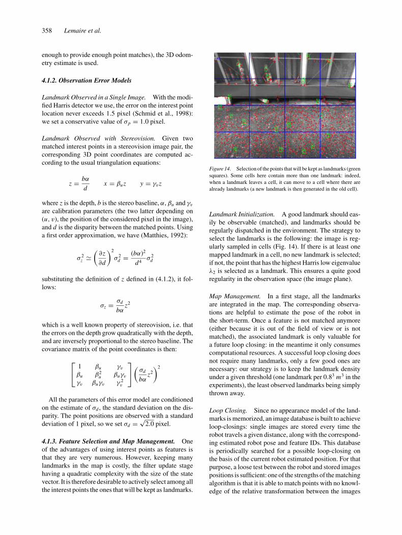
Figure 14. Selection of the points that will be kept as landmarks (green

squares). Some cells here contain more than one landmark: indeed,

when a landmark leaves a cell, it can move to a cell where there are

already landmarks (a new landmark is then generated in the old cell).

Landmark Initialization. A good landmark should eas-ily be observable (matched), and landmarks should beregularly dispatched in the environment. The strategy toselect the landmarks is the following: the image is reg-ularly sampled in cells (Fig. 14). If there is at least onemapped landmark in a cell, no new landmark is selected;if not, the point that has the highest Harris low eigenvalueλ2 is selected as a landmark. This ensures a quite goodregularity in the observation space (the image plane).

Map Management. In a first stage, all the landmarksare integrated in the map. The corresponding observa-tions are helpful to estimate the pose of the robot inthe short-term. Once a feature is not matched anymore(either because it is out of the field of view or is notmatched), the associated landmark is only valuable fora future loop closing: in the meantime it only consumescomputational resources. A successful loop closing doesnot require many landmarks, only a few good ones arenecessary: our strategy is to keep the landmark densityunder a given threshold (one landmark per 0.83 m3 in theexperiments), the least observed landmarks being simplythrown away.

Loop Closing. Since no appearance model of the land-marks is memorized, an image database is built to achieveloop-closings: single images are stored every time therobot travels a given distance, along with the correspond-ing estimated robot pose and feature IDs. This databaseis periodically searched for a possible loop-closing onthe basis of the current robot estimated position. For thatpurpose, a loose test between the robot and stored imagespositions is sufficient: one of the strengths of the matchingalgorithm is that it is able to match points with no knowl-edge of the relative transformation between the images


0

0.02

0.04

0.06

0.08

0.1

0.12

0.14

0.16

0 100 200 300 400 500

su

m o

f tr

an

sla

tio

n s

td. d

ev.

(m

)

frame index

camera sidewardscamera frontward

0

0.02

0.04

0.06

0.08

0.1

0.12

0.14

0.16

0 100 200 300 400 500

su

m o

f tr

an

sla

tio

n s

td. d

ev.

(m

)

frame index

camera sidewardscamera frontward

Figure 15. Comparison of the estimated uncertainty on the robot pose with cameras looking forward and sideward (left: stereovision SLAM, right:

bearings-only SLAM). The robot follows a circular 6 m diameter circular trajectory during 3 laps.

(only a coarse estimate of the scale change is required,up to a factor of 0.5). When a loop-closing detection oc-curs, the corresponding image found in the database andthe current image are fed to the matching algorithm, andsuccessful matches are used to update the stochastic map.

4.1.4. Ground Truth. In the absence of precise devicesthat provide a reference position (such as a centimeter ac-curacy differential GPS), it is difficult to obtain a groundtruth for the robot position along a whole trajectory. How-ever, one can have a fairly precise estimate of the truerover position with respect to its starting position when itcomes back near its starting position at time t , using theVME technique applied to the stereo pairs acquired at thefirst and current positions. VME then provides the currentposition with respect to the starting point, independentlyfrom the achieved trajectory: this position estimate canbe used as a “ground truth” to estimate SLAM errors attime t .

0

50

100

150

200

250

300

350

400

0 100 200 300 400 500

num

ber

of la

ndm

ark

s

frame index

stereo SLAM sidewardsstereo SLAM frontward

boSLAM sidewardsboSLAM frontward

0

100

200

300

400

500

600

700

800

900

0 100 200 300 400 500

num

ber

of tr

acked featu

res

frame index

stereo SLAMboSLAM

Figure 16. Number of mapped landmarks (left) and number of tracked features (right) during stereovision SLAM and bearings-only SLAM (sideward

camera setup).

4.2. Results with a Ground Rover

This section presents results obtained using data ac-quired with the rover Dala, equipped with a 0.35 m widestereo bench mounted on a pan-tilt unit (the images aredown-sampled to a resolution of 512 × 384). The StereoSLAM setup is straightforward, the motion estimate com-puted with VME is used as the prediction input. For thebearings-only SLAM, only the left images of the stereopairs are used, and odometry is used as the predictioninput.

4.2.1. Qualitative Results. Data acquired along a sim-ple 3-loop circular trajectory with a diameter of 6 m pro-vide insights on the behavior of the algorithms. Two setsof data are compared here: one with the cameras lookingforward, and one with the cameras heading sideward.

Figures 15 and 16-left respectively illustrate the evolu-tion of the estimated robot pose standard deviations and

360 Lemaire et al.

-10

-8

-6

-4

-2

0

2

4

6

8

-5 0 5 10 15 20 25

y (

m)

x (m)

VME onlystereoSLAM

-10

-8

-6

-4

-2

0

2

4

6

8

-5 0 5 10 15 20 25

y (

m)

x (m)

odometry onlyboSLAM

Figure 17. Left: trajectories obtained with VME integration and stereo SLAM. Right: trajectories obtained with odometry integration and bearings-

only SLAM (sideward camera setup).

Figure 18. Bearings-only SLAM loop closing: orthogonal projection of the landmarks (3σ ellipses) just before closing the first loop (left) and just

after the first loop (right). The grid step is 1 meter.

number of mapped landmarks. They exhibit the usualloop-closing effects of SLAM: the uncertainty on therobot pose dramatically drops after the first lap, and thenumber of mapped landmarks stops growing once thefrist loop is closed.

The plots also exhibit better performance with thesideward setup than with the forward setup. Indeed,when the cameras are looking sideward, the featuresare tracked on more frames: the mapped landmarksare more often observed, and fewer landmarks areselected. And in the bearings-only case, the side-ward setup yields a greater baseline between consec-utive images, the landmarks are therefore initializedfaster.

Finally, according to these plots bearings-only SLAMseems to perform better than stereo SLAM, in terms ofrobot position precision and number of mapped land-marks. This is actually due to the fact that in stereo

SLAM, a feature needs to be matched between imagest − 1 and t and between the left and right images. Ascan be seen on Fig. 16-right, there are some frames onwhich few features are matched, which reduces the num-ber of observations—note that the frame indices wherefew features are matched correspond to the frame in-dices of Fig. 15-left where the robot pose uncertaintyraises.

4.2.2. Quantitative Results. Results are now presentedon data acquired on a 100 m long trajectory during whichtwo loop closures occur, for both the stereovision andbearings-only cases, the cameras being oriented sideward(Fig. 17).

Loop-Closing Analysis. Figure 18 presents an overviewof the map obtained with bearings-only SLAM at differ-ent points of the trajectory. The landmarks uncertainties


0

2

4

6

8

10

12

14

16

400 450 500 550 600 650 700

num

ber

of m

atc

hes

frame index

loop closing detection (y/n)stereoSLAM

boSLAM

0

0.2

0.4

0.6

0.8

1

1.2

1.4

1.6

0 100 200 300 400 500 600 700

sum

of tr

ansla

tion s

td. dev.

(m

)

frame index

stereoSLAMboSLAM

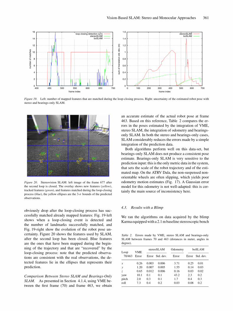
Figure 19. Left: number of mapped features that are matched during the loop-closing process. Right: uncertainty of the estimated robot pose with

stereo and bearings-only SLAM.

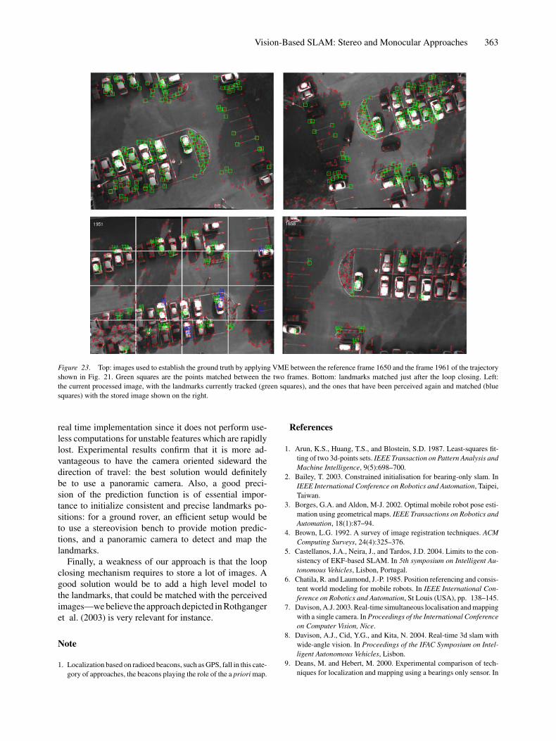
Figure 20. Stereovision SLAM: left image of the frame 677 after

the second loop is closed. The overlay shows new features (yellow),

tracked features (green), and features matched during the loop-closing

process (blue), the yellow ellipses are the 3-σ bounds of the predicted

observations.

obviously drop after the loop-closing process has suc-cessfully matched already mapped features: Fig. 19-leftshows when a loop-closing event is detected andthe number of landmarks successfully matched, andFig. 19-right show the evolution of the robot pose un-certainty. Figure 20 shows the features used by SLAM,after the second loop has been closed. Blue featuresare the ones that have been mapped during the begin-ning of the trajectory and that are “recovered” by theloop-closing process: note that the predicted observa-tions are consistent with the real observations, the de-tected features lie in the ellipses that represents theirprediction.

Comparison Between Stereo SLAM and Bearings-OnlySLAM. As presented in Section 4.1.4, using VME be-tween the first frame (70) and frame 463, we obtain

an accurate estimate of the actual robot pose at frame463. Based on this reference, Table 2 compares the er-rors in the poses estimated by the integration of VME,stereo SLAM, the integration of odometry and bearings-only SLAM. In both the stereo and bearings-only cases,SLAM considerably reduces the errors made by a simpleintegration of the prediction data.

Both algorithms perform well on this data-set, butbearings-only SLAM does not produce a consistent poseestimate. Bearings-only SLAM is very sensitive to theprediction input: this is the only metric data in the system,that sets the scale of the robot trajectory and of the esti-mated map. On the ATRV Dala, the non-suspensed non-orientable wheels are often slipping, which yields poorodometry motion estimates (Fig. 17). A Gaussian errormodel for this odometry is not well-adapted: this is cer-tainly the main source of inconsistency here.

4.3. Results with a Blimp

We ran the algorithms on data acquired by the blimpKarma equipped with a 2.1 m baseline stereoscopic bench

Table 2. Errors made by VME, stereo SLAM and bearings-only

SLAM between frames 70 and 463 (distances in meter, angles in

degree).

stereoSLAM Odometry boSLAMLoop VME

70/463 Error Error Std. dev. Error Error Std. dev.

x 0.26 0.003 0.006 3.71 0.25 0.01

y 1.20 0.007 0.005 1.55 0.14 0.03

z 0.65 0.012 0.006 0.16 0.03 0.02

yaw 10.1 0.1 0.1 43.2 2.3 0.2

pitch 2.0 0.3 0.1 1.7 0.4 0.3

roll 7.3 0.4 0.2 0.03 0.08 0.2

362 Lemaire et al.

Z (m)

VME only

VME + stereoSLAM

2

40

35

30

25

20

15

Y (

m)

Y (m)

-50

510

1520

2530

3540 20

400 –20 –40

–60 –80 –100

X (m)

X (m)

VME only

VME + stereoSLAM

10

5

0

–5–100 –80 –60 –40 –20 0 20 40

0–2–4–6–8

–10–12–14–16–18

Figure 21. Comparison of the trajectory estimated by VME and stereo SLAM (3D view and projection on the ground). The trajectory is about

280 m long, and about 400 image frames have been processed.

Figure 22. The digital elevation map built with dense stereovision

and stereo SLAM trajectory estimate (the grid step is 10 meters).

(Fig. 1), using VME estimates as prediction for boththe stereovision and bearings-only cases (Karma is notequipped with any ego-motion sensor). Figure 21 showsthe trajectories estimated with VME only and with thestereo SLAM approach, and Fig. 22 shows a digital ter-rain map reconstructed using dense stereovision and thepositions estimates provided by SLAM.

Table 3 compares the errors in the poses estimated bythe integration of VME, stereo SLAM, and bearings-onlySLAM, with the “ground truth” provided by the applica-tion of VME between frames 1650 and 1961 (Fig. 23).Here, the position resulting from the integration of VMEexhibits a serious drift in the elevation estimate, a driftthat is properly corrected by SLAM. Nevertheless, bothSLAM approaches do not provide a consistent pose esti-mate: this is a well known problem of SLAM-EKF, thatis sensitive to modeling and linearization errors (Castel-lanos et al., 2004). For large scale SLAM, one shouldswitch to one of the existing algorithm that copes with it,

Table 3. Loop closing results with the blimp (distances in meter, an-

gles in degree).

stereoSLAM boSLAMLoop VME

1650/1961 Error Error Std. dev. Error Std. dev.

x 1.01 9.65 0.15 9.11 0.27

y 4.11 1.35 0.13 1.87 0.16

z 13.97 0.64 0.07 1.68 0.20

yaw 4.26 1.95 0.22 4.49 0.26

pitch 5.70 0.56 0.42 1.24 0.47

roll 7.66 0.2 0.16 0.59 0.24

such as hierarchical approaches which can use a differentoptimization framework than EKF for closing large loops(Estrada et al., 2005).

5. Conclusion

We presented two complete vision based SLAM solu-tions: a classic EKF-SLAM using stereovision observa-tions, and a bearing-only SLAM algorithm that relies onmonocular vision. Both solutions are built upon the sameperception algorithm, which has interesting properties forSLAM: it can match features between images only with acoarse estimation of scale change, which enables to suc-cessfully close large loops. This would not be possiblewith a classic Mahalanobis data association for stereovi-sion, and even more difficult for monocular vision.

As compared to Se et al. (2002), not so many land-marks are stored in the map, and loop closing is success-fully achieved with a low number of landmarks (see Fig.19): a good practical strategy for map management isessential, as it reduces the computation requirements ofseveral parts of the whole SLAM process.

The presented bearing-only algorithm shows a quitegood behavior with real world long range data. Inparticular, the delayed approach is well adapted to a


Figure 23. Top: images used to establish the ground truth by applying VME between the reference frame 1650 and the frame 1961 of the trajectory

shown in Fig. 21. Green squares are the points matched between the two frames. Bottom: landmarks matched just after the loop closing. Left:

the current processed image, with the landmarks currently tracked (green squares), and the ones that have been perceived again and matched (blue

squares) with the stored image shown on the right.

real time implementation since it does not perform use-less computations for unstable features which are rapidlylost. Experimental results confirm that it is more ad-vantageous to have the camera oriented sideward thedirection of travel: the best solution would definitelybe to use a panoramic camera. Also, a good preci-sion of the prediction function is of essential impor-tance to initialize consistent and precise landmarks po-sitions: for a ground rover, an efficient setup would beto use a stereovision bench to provide motion predic-tions, and a panoramic camera to detect and map thelandmarks.

Finally, a weakness of our approach is that the loopclosing mechanism requires to store a lot of images. Agood solution would be to add a high level model tothe landmarks, that could be matched with the perceivedimages—we believe the approach depicted in Rothgangeret al. (2003) is very relevant for instance.

Note

1. Localization based on radioed beacons, such as GPS, fall in this cate-

gory of approaches, the beacons playing the role of the a priori map.

References

1. Arun, K.S., Huang, T.S., and Blostein, S.D. 1987. Least-squares fit-

ting of two 3d-points sets. IEEE Transaction on Pattern Analysis andMachine Intelligence, 9(5):698–700.

2. Bailey, T. 2003. Constrained initialisation for bearing-only slam. In

IEEE International Conference on Robotics and Automation, Taipei,

Taiwan.

3. Borges, G.A. and Aldon, M-J. 2002. Optimal mobile robot pose esti-

mation using geometrical maps. IEEE Transactions on Robotics andAutomation, 18(1):87–94.

4. Brown, L.G. 1992. A survey of image registration techniques. ACMComputing Surveys, 24(4):325–376.

5. Castellanos, J.A., Neira, J., and Tardos, J.D. 2004. Limits to the con-

sistency of EKF-based SLAM. In 5th symposium on Intelligent Au-tonomous Vehicles, Lisbon, Portugal.

6. Chatila, R. and Laumond, J.-P. 1985. Position referencing and consis-

tent world modeling for mobile robots. In IEEE International Con-ference on Robotics and Automation, St Louis (USA), pp. 138–145.

7. Davison, A.J. 2003. Real-time simultaneous localisation and mapping

with a single camera. In Proceedings of the International Conferenceon Computer Vision, Nice.

8. Davison, A.J., Cid, Y.G., and Kita, N. 2004. Real-time 3d slam with

wide-angle vision. In Proceedings of the IFAC Symposium on Intel-ligent Autonomous Vehicles, Lisbon.

9. Deans, M. and Hebert, M. 2000. Experimental comparison of tech-

niques for localization and mapping using a bearings only sensor. In

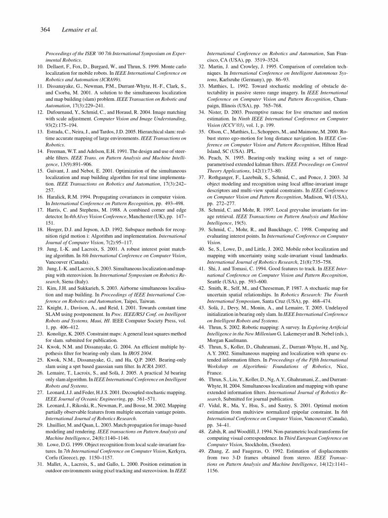
364 Lemaire et al.

Proceedings of the ISER ’00 7th International Symposium on Exper-imental Robotics.

10. Dellaert, F., Fox, D., Burgard, W., and Thrun, S. 1999. Monte carlo

localization for mobile robots. In IEEE International Conference onRobotics and Automation (ICRA99).

11. Dissanayake, G., Newman, P.M., Durrant-Whyte, H.-F., Clark, S.,

and Csorba, M. 2001. A solution to the simultaneous localization

and map building (slam) problem. IEEE Transaction on Robotic andAutomation, 17(3):229–241.

12. Dufournaud, Y., Schmid, C., and Horaud, R. 2004. Image matching

with scale adjustment. Computer Vision and Image Understanding,

93(2):175–194.

13. Estrada, C., Neira, J., and Tardos, J.D. 2005. Hierarchical slam: real-

time accurate mapping of large environments. IEEE Transactions onRobotics.

14. Freeman, W.T. and Adelson, E.H. 1991. The design and use of steer-

able filters. IEEE Trans. on Pattern Analysis and Machine Intelli-gence, 13(9):891–906.

15. Guivant, J. and Nebot, E. 2001. Optimization of the simultaneous

localization and map building algorithm for real time implementa-

tion. IEEE Transactions on Robotics and Automation, 17(3):242–

257.

16. Haralick, R.M. 1994. Propagating covariances in computer vision.

In International Conference on Pattern Recognition, pp. 493–498.

17. Harris, C. and Stephens, M. 1988. A combined corner and edge

detector. In 4th Alvey Vision Conference, Manchester (UK), pp. 147–

151.

18. Heeger, D.J. and Jepson, A.D. 1992. Subspace methods for recog-

nition rigid motion i: Algorithm and implementation. InternationalJournal of Computer Vision, 7(2):95–117.

19. Jung, I.-K. and Lacroix, S. 2001. A robust interest point match-

ing algorithm. In 8th International Conference on Computer Vision,

Vancouver (Canada).

20. Jung, I.-K. and Lacroix, S. 2003. Simultaneous localization and map-

ping with stereovision. In International Symposium on Robotics Re-search, Siena (Italy).

21. Kim, J.H. and Sukkarieh, S. 2003. Airborne simultaneous localisa-

tion and map building. In Proceedings of IEEE International Con-ference on Robotics and Automation, Taipei, Taiwan.

22. Knight, J., Davison, A., and Reid, I. 2001. Towards constant time

SLAM using postponement. In Proc. IEEE/RSJ Conf. on IntelligentRobots and Systems, Maui, HI. IEEE Computer Society Press, vol.

1, pp. 406–412.

23. Konolige, K. 2005. Constraint maps: A general least squares method

for slam. submited for publication.

24. Kwok, N.M. and Dissanayake, G. 2004. An efficient multiple hy-

pothesis filter for bearing-only slam. In IROS 2004.

25. Kwok, N.M., Dissanayake, G., and Ha, Q.P. 2005. Bearing-only

slam using a sprt based gaussian sum filter. In ICRA 2005.

26. Lemaire, T., Lacroix, S., and Sola, J. 2005. A practical 3d bearing

only slam algorithm. In IEEE International Conference on IntelligentRobots and Systems.

27. Leonard, J.J. and Feder, H.J.S. 2001. Decoupled stochastic mapping.

IEEE Journal of Oceanic Engineering, pp. 561–571.

28. Leonard, J., Rikoski, R., Newman, P., and Bosse, M. 2002. Mapping

partially observable features from multiple uncertain vantage points.

International Journal of Robotics Research.

29. Lhuillier, M. and Quan, L. 2003. Match propagation for image-based

modeling and rendering. IEEE transactions on Pattern Analysis andMachine Intelligence, 24(8):1140–1146.

30. Lowe, D.G. 1999. Object recognition from local scale-invariant fea-

tures. In 7th International Conference on Computer Vision, Kerkyra,

Corfu (Greece), pp. 1150–1157.

31. Mallet, A., Lacroix, S., and Gallo, L. 2000. Position estimation in

outdoor environments using pixel tracking and stereovision. In IEEE

International Conference on Robotics and Automation, San Fran-

cisco, CA (USA), pp. 3519–3524.

32. Martin, J. and Crowley, J. 1995. Comparison of correlation tech-

niques. In International Conference on Intelligent Autonmous Sys-tems, Karlsruhe (Germany), pp. 86–93.

33. Matthies, L. 1992. Toward stochastic modeling of obstacle de-

tectability in passive stereo range imagery. In IEEE InternationalConference on Computer Vision and Pattern Recognition, Cham-

paign, Illinois (USA), pp. 765–768.

34. Nister, D. 2003. Preemptive ransac for live structure and motion

estimation. In Ninth IEEE International Conference on ComputerVision (ICCV’03), vol. 1, p. 199.

35. Olson, C., Matthies, L., Schoppers, M., and Maimone, M. 2000. Ro-

bust stereo ego-motion for long distance navigation. In IEEE Con-ference on Computer Vision and Pattern Recognition, Hilton Head

Island, SC (USA). JPL.

36. Peach, N. 1995. Bearing-only tracking using a set of range-

parametrised extended kalman filters. IEEE Proceedings on ControlTheory Applications, 142(1):73–80.

37. Rothganger, F., Lazebnik, S., Schmid, C., and Ponce, J. 2003. 3d

object modeling and recognition using local affine-invariant image

descriptors and multi-view spatial constraints. In IEEE Conferenceon Computer Vision and Pattern Recognition, Madison, WI (USA),

pp. 272–277.

38. Schmid, C. and Mohr, R. 1997. Local greyvalue invariants for im-

age retrieval. IEEE Transactions on Pattern Analysis and MachineIntelligence, 19(5).

39. Schmid, C., Mohr, R., and Bauckhage, C. 1998. Comparing and

evaluating interest points. In International Conference on ComputerVision.

40. Se, S., Lowe, D., and Little, J. 2002. Mobile robot localization and

mapping with uncertainty using scale-invariant visual landmarks.

International Journal of Robotics Research, 21(8):735–758.

41. Shi, J. and Tomasi, C. 1994. Good features to track. In IEEE Inter-national Conference on Computer Vision and Pattern Recognition,

Seattle (USA), pp. 593–600.

42. Smith, R., Self, M., and Cheeseman, P. 1987. A stochastic map for

uncertain spatial relationships. In Robotics Research: The FourthInternational Symposium, Santa Cruz (USA), pp. 468–474.

43. Sola, J., Devy, M., Monin, A., and Lemaire, T. 2005. Undelayed

initialization in bearing only slam. In IEEE International Conferenceon Intelligent Robots and Systems.

44. Thrun, S. 2002. Robotic mapping: A survey. In Exploring ArtificialIntelligence in the New Millenium G. Lakemeyer and B. Nebel (eds.),

Morgan Kaufmann.

45. Thrun, S., Koller, D., Ghahramani, Z., Durrant-Whyte, H., and Ng,

A.Y. 2002. Simultaneous mapping and localization with sparse ex-

tended information filters. In Proceedings of the Fifth InternationalWorkshop on Algorithmic Foundations of Robotics, Nice,

France.

46. Thrun, S., Liu, Y., Koller, D., Ng, A.Y., Ghahramani, Z., and Durrant-

Whyte, H. 2004. Simultaneous localization and mapping with sparse

extended information filters. International Journal of Robotics Re-search, Submitted for journal publication.

47. Vidal, R., Ma, Y., Hsu, S., and Sastry, S. 2001. Optimal motion

estimation from multiview normalized epipolar constraint. In 8thInternational Conference on Computer Vision, Vancouver (Canada),

pp. 34–41.

48. Zabih, R. and Woodfill, J. 1994. Non-parametric local transforms for

computing visual correspondence. In Third European Conference onComputer Vision, Stockholm, (Sweden).

49. Zhang, Z. and Faugeras, O. 1992. Estimation of displacements

from two 3-D frames obtained from stereo. IEEE Transac-tions on Pattern Analysis and Machine Intelligence, 14(12):1141–

1156.

Vision-Based SLAM: Stereo and Monocular …mdailey/cvreadings/Lemaire-SLAM.pdf · Vision-Based SLAM: Stereo and Monocular Approaches 345 Figure 1.The ATRV rover Dala and the 10 m

Documents