Video Processing & Communications - Wang
Oct 14, 2014
Welcome message from author
This document is posted to help you gain knowledge. Please leave a comment to let me know what you think about it! Share it to your friends and learn new things together.
Transcript
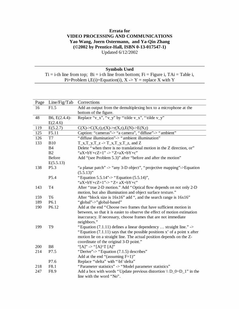
Errata for VIDEO PROCESSING AND COMMUNICATIONS
Yao Wang, Joern Ostermann, and Ya-Qin Zhang (©2002 by Prentice-Hall, ISBN 0-13-017547-1)
Updated 6/12/2002
Symbols Used Ti = i-th line from top; Bi = i-th line from bottom; Fi = Figure i, TAi = Table i,
Pi=Problem i,E(i)=Equation(i), X -> Y = replace X with Y
Page Line/Fig/Tab Corrections 16 F1.5 Add an output from the demultiplexing box to a microphone at the
bottom of the figure. 48 B6, E(2.4.4)-
E(2.4.6) Replace “v_x”, “v_y” by “\tilde v_x”, “\tilde v_y”
119 E(5.2.7) C(X)->C(X,t),r(X)->r(X,t),E(N)->E(N,t) 125 F5.11 Caption: “cameras”-> “a camera”, “diffuse”-> “ambient” 126 T7 “diffuse illumination”-> “ambient illumination” 133 B10 T_x,T_y,T_z -> T_x,T_y,T_z, and Z B4 Delete “when there is no translational motion in the Z direction, or” B2 “aX+bY+cZ=1” -> “Z=aX+bY+c” Before
E(5.5.13) Add “(see Problem 5.3)” after “before and after the motion”
138 P5.3 “a planar patch” -> “any 3-D object”, “projective mapping”->Equation (5.5.13)”
P5.4 “Equation 5.5.14”-> “Equation (5.5.14)”, “aX+bY+cZ=1”-> “Z= aX+bY+c”
143 T4 After “true 2-D motion.” Add “Optical flow depends on not only 2-D motion, but also illumination and object surface texture.”
159 T6 After “block size is 16x16” add “, and the search range is 16x16” 189 P6.1 “global”->”global-based” 190 P6.12 Add at the end “Choose two frames that have sufficient motion in
between, so that it is easier to observe the effect of motion estimation inaccuracy. If necessary, choose frames that are not immediate neighbors.”
199 T9 “Equation (7.1.11) defines a linear dependency … straight line.” -> “Equation (7.1.11) says that the possible positions x’ of a point x after motion lie on a straight line. The actual position depends on the Z-coordinate of the original 3-D point.”
200 B8 “[A]” -> “[A]^T [A]” 214 P7.5 “Derive”-> “Equation (7.1.5) describes”
Add at the end “(assuming F=1)” P7.6 Replace “\delta” with “\bf \delta” 218 F8.1 “Parameter statistics” -> “Model parameter statistics” 247 F8.9 Add a box with words “Update previous distortion \\ D_0=D_1” in the
line with the word “No”.

255 F8.14 Same as for F8.9 261 P8.13(a) “B_l={f_k, k=1,2,… ,K_l}” -> “B_l, which consists of K_l vectors in
{\cal F}” 416 TA13.2 Item “4CIF/H.263” should be “Opt.” 421 TA13.3 Item “Video/Non-QoS LAN” should be “H.261/3” 436 T13 “MPEG-2, defined” -> “MPEG-2 defined” 443 T10 “I-VOP”->”I-VOPs”, “B-VOP”-> “B-VOPs” 575 P1.3 “red+green=blue”-> “red+green=black” P1.4 “(1.4.4)” -> “(1.4.3)”, “(1.4.2)” -> “(1.4.1)”
wang-50214 wang˙fm August 23, 2001 14:22
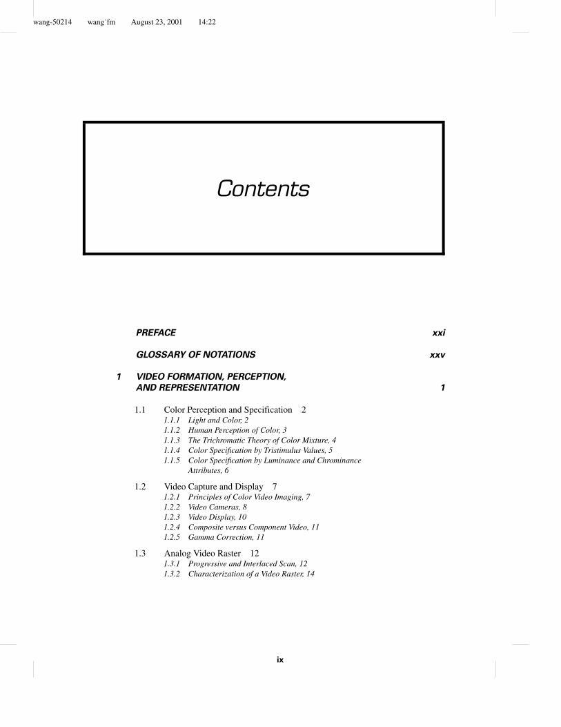
Contents
PREFACE xxi
GLOSSARY OF NOTATIONS xxv
1 VIDEO FORMATION, PERCEPTION,
AND REPRESENTATION 1
1.1 Color Perception and Specification 21.1.1 Light and Color, 21.1.2 Human Perception of Color, 31.1.3 The Trichromatic Theory of Color Mixture, 41.1.4 Color Specification by Tristimulus Values, 51.1.5 Color Specification by Luminance and Chrominance
Attributes, 6
1.2 Video Capture and Display 71.2.1 Principles of Color Video Imaging, 71.2.2 Video Cameras, 81.2.3 Video Display, 101.2.4 Composite versus Component Video, 111.2.5 Gamma Correction, 11
1.3 Analog Video Raster 121.3.1 Progressive and Interlaced Scan, 121.3.2 Characterization of a Video Raster, 14
ix
wang-50214 wang˙fm August 23, 2001 14:22
x Contents
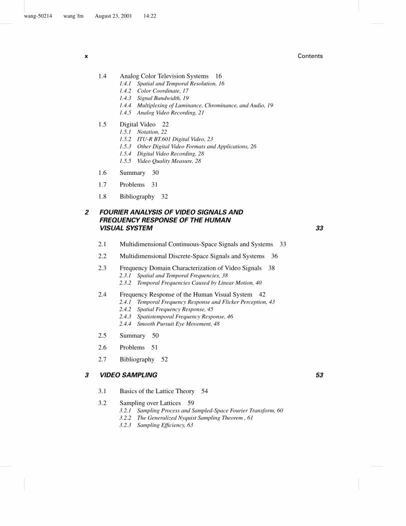
1.4 Analog Color Television Systems 161.4.1 Spatial and Temporal Resolution, 161.4.2 Color Coordinate, 171.4.3 Signal Bandwidth, 191.4.4 Multiplexing of Luminance, Chrominance, and Audio, 191.4.5 Analog Video Recording, 21
1.5 Digital Video 221.5.1 Notation, 221.5.2 ITU-R BT.601 Digital Video, 231.5.3 Other Digital Video Formats and Applications, 261.5.4 Digital Video Recording, 281.5.5 Video Quality Measure, 28
1.6 Summary 30
1.7 Problems 31
1.8 Bibliography 32
2 FOURIER ANALYSIS OF VIDEO SIGNALS AND
FREQUENCY RESPONSE OF THE HUMAN
VISUAL SYSTEM 33
2.1 Multidimensional Continuous-Space Signals and Systems 33
2.2 Multidimensional Discrete-Space Signals and Systems 36
2.3 Frequency Domain Characterization of Video Signals 382.3.1 Spatial and Temporal Frequencies, 382.3.2 Temporal Frequencies Caused by Linear Motion, 40
2.4 Frequency Response of the Human Visual System 422.4.1 Temporal Frequency Response and Flicker Perception, 432.4.2 Spatial Frequency Response, 452.4.3 Spatiotemporal Frequency Response, 462.4.4 Smooth Pursuit Eye Movement, 48
2.5 Summary 50
2.6 Problems 51
2.7 Bibliography 52
3 VIDEO SAMPLING 53
3.1 Basics of the Lattice Theory 54
3.2 Sampling over Lattices 593.2.1 Sampling Process and Sampled-Space Fourier Transform, 603.2.2 The Generalized Nyquist Sampling Theorem , 613.2.3 Sampling Efficiency, 63
wang-50214 wang˙fm August 23, 2001 14:22
Contents xi
3.2.4 Implementation of the Prefilter and Reconstruction Filter, 653.2.5 Relation between Fourier Transforms over Continuous, Discrete,
and Sampled Spaces, 66
3.3 Sampling of Video Signals 673.3.1 Required Sampling Rates, 673.3.2 Sampling Video in Two Dimensions: Progressive versus
Interlaced Scans, 693.3.3 Sampling a Raster Scan: BT.601 Format Revisited, 713.3.4 Sampling Video in Three Dimensions, 723.3.5 Spatial and Temporal Aliasing, 73
3.4 Filtering Operations in Cameras and Display Devices 763.4.1 Camera Apertures, 763.4.2 Display Apertures, 79
3.5 Summary 80
3.6 Problems 80
3.7 Bibliography 83
4 VIDEO SAMPLING RATE CONVERSION 84
4.1 Conversion of Signals Sampled on Different Lattices 844.1.1 Up-Conversion, 854.1.2 Down-Conversion, 874.1.3 Conversion between Arbitrary Lattices, 894.1.4 Filter Implementation and Design, and Other Interpolation
Approaches, 91
4.2 Sampling Rate Conversion of Video Signals 924.2.1 Deinterlacing, 934.2.2 Conversion between PAL and NTSC Signals, 984.2.3 Motion-Adaptive Interpolation, 104
4.3 Summary 105
4.4 Problems 106
4.5 Bibliography 109
5 VIDEO MODELING 111
5.1 Camera Model 1125.1.1 Pinhole Model, 1125.1.2 CAHV Model, 1145.1.3 Camera Motions, 116
5.2 Illumination Model 1165.2.1 Diffuse and Specular Reflection, 116
wang-50214 wang˙fm August 23, 2001 14:22
xii Contents
5.2.2 Radiance Distribution under Differing Illumination and ReflectionConditions, 117
5.2.3 Changes in the Image Function Due to Object Motion, 119
5.3 Object Model 1205.3.1 Shape Model, 1215.3.2 Motion Model, 122
5.4 Scene Model 125
5.5 Two-Dimensional Motion Models 1285.5.1 Definition and Notation, 1285.5.2 Two-Dimensional Motion Models Corresponding to Typical Camera
Motions, 1305.5.3 Two-Dimensional Motion Corresponding to Three-Dimensional Rigid
Motion, 1335.5.4 Approximations of Projective Mapping, 136
5.6 Summary 137
5.7 Problems 138
5.8 Bibliography 139
6 TWO-DIMENSIONAL MOTION ESTIMATION 141
6.1 Optical Flow 1426.1.1 Two-Dimensional Motion versus Optical Flow, 1426.1.2 Optical Flow Equation and Ambiguity in Motion Estimation, 143
6.2 General Methodologies 1456.2.1 Motion Representation, 1466.2.2 Motion Estimation Criteria, 1476.2.3 Optimization Methods, 151
6.3 Pixel-Based Motion Estimation 1526.3.1 Regularization Using the Motion Smoothness Constraint, 1536.3.2 Using a Multipoint Neighborhood, 1536.3.3 Pel-Recursive Methods, 154
6.4 Block-Matching Algorithm 1546.4.1 The Exhaustive Block-Matching Algorithm, 1556.4.2 Fractional Accuracy Search, 1576.4.3 Fast Algorithms, 1596.4.4 Imposing Motion Smoothness Constraints, 1616.4.5 Phase Correlation Method, 1626.4.6 Binary Feature Matching, 163
6.5 Deformable Block-Matching Algorithms 1656.5.1 Node-Based Motion Representation, 1666.5.2 Motion Estimation Using the Node-Based Model, 167
wang-50214 wang˙fm August 23, 2001 14:22
Contents xiii
6.6 Mesh-Based Motion Estimation 1696.6.1 Mesh-Based Motion Representation, 1716.6.2 Motion Estimation Using the Mesh-Based Model, 173
6.7 Global Motion Estimation 1776.7.1 Robust Estimators, 1776.7.2 Direct Estimation, 1786.7.3 Indirect Estimation, 178
6.8 Region-Based Motion Estimation 1796.8.1 Motion-Based Region Segmentation, 1806.8.2 Joint Region Segmentation and Motion Estimation, 181
6.9 Multiresolution Motion Estimation 1826.9.1 General Formulation, 1826.9.2 Hierarchical Block Matching Algorithm, 184
6.10 Application of Motion Estimation in Video Coding 187
6.11 Summary 188
6.12 Problems 189
6.13 Bibliography 191
7 THREE-DIMENSIONAL MOTION ESTIMATION 194
7.1 Feature-Based Motion Estimation 1957.1.1 Objects of Known Shape under Orthographic Projection, 1957.1.2 Objects of Known Shape under Perspective Projection, 1967.1.3 Planar Objects, 1977.1.4 Objects of Unknown Shape Using the Epipolar Line, 198
7.2 Direct Motion Estimation 2037.2.1 Image Signal Models and Motion, 2047.2.2 Objects of Known Shape, 2067.2.3 Planar Objects, 2077.2.4 Robust Estimation, 209
7.3 Iterative Motion Estimation 212
7.4 Summary 213
7.5 Problems 214
7.6 Bibliography 215
8 FOUNDATIONS OF VIDEO CODING 217
8.1 Overview of Coding Systems 2188.1.1 General Framework, 2188.1.2 Categorization of Video Coding Schemes, 219
wang-50214 wang˙fm August 23, 2001 14:22
xiv Contents
8.2 Basic Notions in Probability and Information Theory 2218.2.1 Characterization of Stationary Sources, 2218.2.2 Entropy and Mutual Information for Discrete Sources, 2228.2.3 Entropy and Mutual Information for Continuous
Sources, 226
8.3 Information Theory for Source Coding 2278.3.1 Bound for Lossless Coding, 2278.3.2 Bound for Lossy Coding, 2298.3.3 Rate-Distortion Bounds for Gaussian Sources, 232
8.4 Binary Encoding 2348.4.1 Huffman Coding, 2358.4.2 Arithmetic Coding, 238
8.5 Scalar Quantization 2418.5.1 Fundamentals, 2418.5.2 Uniform Quantization, 2438.5.3 Optimal Scalar Quantizer, 244
8.6 Vector Quantization 2488.6.1 Fundamentals, 2488.6.2 Lattice Vector Quantizer, 2518.6.3 Optimal Vector Quantizer, 2538.6.4 Entropy-Constrained Optimal Quantizer Design, 255
8.7 Summary 257
8.8 Problems 259
8.9 Bibliography 261
9 WAVEFORM-BASED VIDEO CODING 263
9.1 Block-Based Transform Coding 2639.1.1 Overview, 2649.1.2 One-Dimensional Unitary Transform, 2669.1.3 Two-Dimensional Unitary Transform, 2699.1.4 The Discrete Cosine Transform, 2719.1.5 Bit Allocation and Transform Coding Gain, 2739.1.6 Optimal Transform Design and the KLT, 2799.1.7 DCT-Based Image Coders and the JPEG Standard, 2819.1.8 Vector Transform Coding, 284
9.2 Predictive Coding 2859.2.1 Overview, 2859.2.2 Optimal Predictor Design and Predictive Coding Gain, 2869.2.3 Spatial-Domain Linear Prediction, 2909.2.4 Motion-Compensated Temporal Prediction, 291
wang-50214 wang˙fm August 23, 2001 14:22
Contents xv
9.3 Video Coding Using Temporal Prediction and Transform Coding 2939.3.1 Block-Based Hybrid Video Coding, 2939.3.2 Overlapped Block Motion Compensation, 2969.3.3 Coding Parameter Selection, 2999.3.4 Rate Control, 3029.3.5 Loop Filtering, 305
9.4 Summary 308
9.5 Problems 309
9.6 Bibliography 311
10 CONTENT-DEPENDENT VIDEO CODING 314
10.1 Two-Dimensional Shape Coding 31410.1.1 Bitmap Coding, 31510.1.2 Contour Coding, 31810.1.3 Evaluation Criteria for Shape Coding Efficiency, 323
10.2 Texture Coding for Arbitrarily Shaped Regions 32410.2.1 Texture Extrapolation, 32410.2.2 Direct Texture Coding, 325
10.3 Joint Shape and Texture Coding 326
10.4 Region-Based Video Coding 327
10.5 Object-Based Video Coding 32810.5.1 Source Model F2D, 33010.5.2 Source Models R3D and F3D, 332
10.6 Knowledge-Based Video Coding 336
10.7 Semantic Video Coding 338
10.8 Layered Coding System 339
10.9 Summary 342
10.10 Problems 343
10.11 Bibliography 344
11 SCALABLE VIDEO CODING 349
11.1 Basic Modes of Scalability 35011.1.1 Quality Scalability, 35011.1.2 Spatial Scalability, 35311.1.3 Temporal Scalability, 35611.1.4 Frequency Scalability, 356
wang-50214 wang˙fm August 23, 2001 14:22
xvi Contents
11.1.5 Combination of Basic Schemes, 35711.1.6 Fine-Granularity Scalability, 357
11.2 Object-Based Scalability 359
11.3 Wavelet-Transform-Based Coding 36111.3.1 Wavelet Coding of Still Images, 36311.3.2 Wavelet Coding of Video, 367
11.4 Summary 370
11.5 Problems 370
11.6 Bibliography 371
12 STEREO AND MULTIVIEW SEQUENCE PROCESSING 374
12.1 Depth Perception 37512.1.1 Binocular Cues—Stereopsis, 37512.1.2 Visual Sensitivity Thresholds for Depth Perception, 375
12.2 Stereo Imaging Principle 37712.2.1 Arbitrary Camera Configuration, 37712.2.2 Parallel Camera Configuration, 37912.2.3 Converging Camera Configuration, 38112.2.4 Epipolar Geometry, 383
12.3 Disparity Estimation 38512.3.1 Constraints on Disparity Distribution, 38612.3.2 Models for the Disparity Function, 38712.3.3 Block-Based Approach, 38812.3.4 Two-Dimensional Mesh-Based Approach, 38812.3.5 Intra-Line Edge Matching Using Dynamic Programming, 39112.3.6 Joint Structure and Motion Estimation, 392
12.4 Intermediate View Synthesis 393
12.5 Stereo Sequence Coding 39612.5.1 Block-Based Coding and MPEG-2 Multiview Profile, 39612.5.2 Incomplete Three-Dimensional Representation
of Multiview Sequences, 39812.5.3 Mixed-Resolution Coding, 39812.5.4 Three-Dimensional Object-Based Coding, 39912.5.5 Three-Dimensional Model-Based Coding, 400
12.6 Summary 400
12.7 Problems 402
12.8 Bibliography 403

wang-50214 wang˙fm August 23, 2001 14:22
Contents xvii
13 VIDEO COMPRESSION STANDARDS 405
13.1 Standardization 40613.1.1 Standards Organizations, 40613.1.2 Requirements for a Successful Standard, 40913.1.3 Standard Development Process, 41113.1.4 Applications for Modern Video Coding Standards, 412
13.2 Video Telephony with H.261 and H.263 41313.2.1 H.261 Overview, 41313.2.2 H.263 Highlights, 41613.2.3 Comparison, 420
13.3 Standards for Visual Communication Systems 42113.3.1 H.323 Multimedia Terminals, 42113.3.2 H.324 Multimedia Terminals, 422
13.4 Consumer Video Communications with MPEG-1 42313.4.1 Overview, 42313.4.2 MPEG-1 Video, 424
13.5 Digital TV with MPEG-2 42613.5.1 Systems, 42613.5.2 Audio, 42613.5.3 Video, 42713.5.4 Profiles, 435
13.6 Coding of Audiovisual Objects with MPEG-4 43713.6.1 Systems, 43713.6.2 Audio, 44113.6.3 Basic Video Coding, 44213.6.4 Object-Based Video Coding, 44513.6.5 Still Texture Coding, 44713.6.6 Mesh Animation, 44713.6.7 Face and Body Animation, 44813.6.8 Profiles, 45113.6.9 Evaluation of Subjective Video Quality, 454
13.7 Video Bit Stream Syntax 454
13.8 Multimedia Content Description Using MPEG-7 45813.8.1 Overview, 45813.8.2 Multimedia Description Schemes, 45913.8.3 Visual Descriptors and Description Schemes, 461
13.9 Summary 465
13.10 Problems 466
13.11 Bibliography 467
wang-50214 wang˙fm August 23, 2001 14:22
xviii Contents
14 ERROR CONTROL IN VIDEO COMMUNICATIONS 472
14.1 Motivation and Overview of Approaches 473
14.2 Typical Video Applications and Communication Networks 47614.2.1 Categorization of Video Applications, 47614.2.2 Communication Networks, 479
14.3 Transport-Level Error Control 48514.3.1 Forward Error Correction, 48514.3.2 Error-Resilient Packetization and Multiplexing, 48614.3.3 Delay-Constrained Retransmission, 48714.3.4 Unequal Error Protection, 488
14.4 Error-Resilient Encoding 48914.4.1 Error Isolation, 48914.4.2 Robust Binary Encoding, 49014.4.3 Error-Resilient Prediction, 49214.4.4 Layered Coding with Unequal Error Protection, 49314.4.5 Multiple-Description Coding, 49414.4.6 Joint Source and Channel Coding, 498
14.5 Decoder Error Concealment 49814.5.1 Recovery of Texture Information, 50014.5.2 Recovery of Coding Modes and Motion Vectors, 50114.5.3 Syntax-Based Repair, 502
14.6 Encoder–Decoder Interactive Error Control 50214.6.1 Coding-Parameter Adaptation Based on Channel Conditions, 50314.6.2 Reference Picture Selection Based on Feedback Information, 50314.6.3 Error Tracking Based on Feedback Information, 50414.6.4 Retransmission without Waiting, 504
14.7 Error-Resilience Tools in H.263 and MPEG-4 50514.7.1 Error-Resilience Tools in H.263, 50514.7.2 Error-Resilience Tools in MPEG-4, 508
14.8 Summary 509
14.9 Problems 511
14.10 Bibliography 513
15 STREAMING VIDEO OVER THE INTERNET AND
WIRELESS IP NETWORKS 519
15.1 Architecture for Video Streaming Systems 520
15.2 Video Compression 522
wang-50214 wang˙fm August 23, 2001 14:22
Contents xix
15.3 Application-Layer QoS Control for Streaming Video 52215.3.1 Congestion Control, 52215.3.2 Error Control, 525
15.4 Continuous Media Distribution Services 52915.4.1 Network Filtering, 52915.4.2 Application-Level Multicast, 53115.4.3 Content Replication, 532
15.5 Streaming Servers 53315.5.1 Real-Time Operating System, 53415.5.2 Storage System, 537
15.6 Media Synchronization 539
15.7 Protocols for Streaming Video 54215.7.1 Transport Protocols, 54315.7.2 Session Control Protocol: RTSP, 545
15.8 Streaming Video over Wireless IP Networks 54615.8.1 Network-Aware Applications, 54815.8.2 Adaptive Service, 549
15.9 Summary 554
15.10 Bibliography 555
APPENDIX A: DETERMINATION OF SPATIAL–TEMPORAL
GRADIENTS 562
A.1 First- and Second-Order Gradient 562
A.2 Sobel Operator 563
A.3 Difference of Gaussian Filters 563
APPENDIX B: GRADIENT DESCENT METHODS 565
B.1 First-Order Gradient Descent Method 565
B.2 Steepest Descent Method 566
B.3 Newton’s Method 566
B.4 Newton-Ralphson Method 567
B.5 Bibliography 567
APPENDIX C: GLOSSARY OF ACRONYMS 568
APPENDIX D: ANSWERS TO SELECTED PROBLEMS 575

wang-50214 wang˙fm August 23, 2001 14:22
xx
wang-50214 wang˙fm August 23, 2001 14:22
Preface
In the past decade or so, there have been fascinating developments in multimedia rep-resentation and communications. First of all, it has become very clear that all aspectsof media are “going digital”; from representation to transmission, from processing toretrieval, from studio to home. Second, there have been significant advances in digitalmultimedia compression and communication algorithms, which make it possible todeliver high-quality video at relatively low bit rates in today’s networks. Third, theadvancement in VLSI technologies has enabled sophisticated software to be imple-mented in a cost-effective manner. Last but not least, the establishment of half a dozeninternational standards by ISO/MPEG and ITU-T laid the common groundwork fordifferent vendors and content providers.
At the same time, the explosive growth in wireless and networking technologyhas profoundly changed the global communications infrastructure. It is the confluenceof wireless, multimedia, and networking that will fundamentally change the way peopleconduct business and communicate with each other. The future computing and com-munications infrastructure will be empowered by virtually unlimited bandwidth, fullconnectivity, high mobility, and rich multimedia capability.
As multimedia becomes more pervasive, the boundaries between video, graphics,computer vision, multimedia database, and computer networking start to blur, makingvideo processing an exciting field with input from many disciplines. Today, videoprocessing lies at the core of multimedia. Among the many technologies involved, videocoding and its standardization are definitely the key enablers of these developments.This book covers the fundamental theory and techniques for digital video processing,with a focus on video coding and communications. It is intended as a textbook for agraduate-level course on video processing, as well as a reference or self-study text for
xxi
wang-50214 wang˙fm August 23, 2001 14:22
xxii Preface
researchers and engineers. In selecting the topics to cover, we have tried to achievea balance between providing a solid theoretical foundation and presenting complexsystem issues in real video systems.
SYNOPSIS
Chapter 1 gives a broad overview of video technology, from analog color TV sys-tem to digital video. Chapter 2 delineates the analytical framework for video analysisin the frequency domain, and describes characteristics of the human visual system.Chapters 3–12 focus on several very important sub-topics in digital video technology.Chapters 3 and 4 consider how a continuous-space video signal can be sampled toretain the maximum perceivable information within the affordable data rate, and howvideo can be converted from one format to another. Chapter 5 presents models forthe various components involved in forming a video signal, including the camera, theillumination source, the imaged objects and the scene composition. Models for thethree-dimensional (3-D) motions of the camera and objects, as well as their projectionsonto the two-dimensional (2-D) image plane, are discussed at length, because thesemodels are the foundation for developing motion estimation algorithms, which arethe subjects of Chapters 6 and 7. Chapter 6 focuses on 2-D motion estimation, whichis a critical component in modern video coders. It is also a necessary preprocessingstep for 3-D motion estimation. We provide both the fundamental principles governing2-D motion estimation, and practical algorithms based on different 2-D motion repre-sentations. Chapter 7 considers 3-D motion estimation, which is required for variouscomputer vision applications, and can also help improve the efficiency of video coding.
Chapters 8–11 are devoted to the subject of video coding. Chapter 8 introducesthe fundamental theory and techniques for source coding, including information theorybounds for both lossless and lossy coding, binary encoding methods, and scalar andvector quantization. Chapter 9 focuses on waveform-based methods (including trans-form and predictive coding), and introduces the block-based hybrid coding framework,which is the core of all international video coding standards. Chapter 10 discussescontent-dependent coding, which has the potential of achieving extremely high com-pression ratios by making use of knowledge of scene content. Chapter 11 presentsscalable coding methods, which are well-suited for video streaming and broadcast-ing applications, where the intended recipients have varying network connections andcomputing powers. Chapter 12 introduces stereoscopic and multiview video processingtechniques, including disparity estimation and coding of such sequences.
Chapters 13–15 cover system-level issues in video communications. Chapter 13introduces the H.261, H.263, MPEG-1, MPEG-2, and MPEG-4 standards for videocoding, comparing their intended applications and relative performance. These stan-dards integrate many of the coding techniques discussed in Chapters 8–11. The MPEG-7standard for multimedia content description is also briefly described. Chapter 14 reviewstechniques for combating transmission errors in video communication systems, andalso describes the requirements of different video applications, and the characteristics
wang-50214 wang˙fm August 23, 2001 14:22
Preface xxiii
of various networks. As an example of a practical video communication system, weend the text with a chapter devoted to video streaming over the Internet and wirelessnetwork. Chapter 15 discusses the requirements and representative solutions for themajor subcomponents of a streaming system.
SUGGESTED USE FOR INSTRUCTION AND SELF-STUDY
As prerequisites, students are assumed to have finished undergraduate courses in signalsand systems, communications, probability, and preferably a course in image process-ing. For a one-semester course focusing on video coding and communications, werecommend covering the two beginning chapters, followed by video modeling (Chap-ter 5), 2-D motion estimation (Chapter 6), video coding (Chapters 8–11), standards(Chapter 13), error control (Chapter 14) and video streaming systems (Chapter 15).On the other hand, for a course on general video processing, the first nine chapters, in-cluding the introduction (Chapter 1), frequency domain analysis (Chapter 2), samplingand sampling rate conversion (Chapters 3 and 4), video modeling (Chapter 5), motionestimation (Chapters 6 and 7), and basic video coding techniques (Chapters 8 and 9),plus selected topics from Chapters 10–13 (content-dependent coding, scalable coding,stereo, and video coding standards) may be appropriate. In either case, Chapter 8 maybe skipped or only briefly reviewed if the students have finished a prior course onsource coding. Chapters 7 (3-D motion estimation), 10 (content-dependent coding),11 (scalable coding), 12 (stereo), 14 (error-control), and 15 (video streaming) may alsobe left for an advanced course in video, after covering the other chapters in a first coursein video. In all cases, sections denoted by asterisks (*) may be skipped or left for furtherexploration by advanced students.
Problems are provided at the end of Chapters 1–14 for self-study or as home-work assignments for classroom use. Appendix D gives answers to selected problems.The website for this book (www.prenhall.com/wang) provides MATLAB scripts used togenerate some of the plots in the figures. Instructors may modify these scripts to generatesimilar examples. The scripts may also help students to understand the underlyingoperations. Sample video sequences can be downloaded from the website, so thatstudents can evaluate the performance of different algorithms on real sequences. Somecompressed sequences using standard algorithms are also included, to enable instructorsto demonstrate coding artifacts at different rates by different techniques.
ACKNOWLEDGMENTS
We are grateful to the many people who have helped to make this book a reality. Dr.Barry G. Haskell of AT&T Labs, with his tremendous experience in video coding stan-dardization, reviewed Chapter 13 and gave valuable input to this chapter as well as othertopics. Prof. David J. Goodman of Polytechnic University, a leading expert in wirelesscommunications, provided valuable input to Section 14.2.2, part of which summarizecharacteristics of wireless networks. Prof. Antonio Ortega of the University of Southern
wang-50214 wang˙fm August 23, 2001 14:22
xxiv Preface
California and Dr. Anthony Vetro of Mitsubishi Electric Research Laboratories, thena Ph.D. student at Polytechnic University, suggested what topics to cover in the sec-tion on rate control, and reviewed Sections 9.3.3–4. Mr. Dapeng Wu, a Ph.D. studentat Carnegie Mellon University, and Dr. Yiwei Hou from Fijitsu Labs helped to draftChapter 15. Dr. Ru-Shang Wang of Nokia Research Center, Mr. Fatih Porikli of Mit-subishi Electric Research Laboratories, also a Ph.D. student at Polytechnic University,and Mr. Khalid Goudeaux, a student at Carnegie Mellon University, generated severalimages related to stereo. Mr. Haidi Gu, a student at Polytechnic University, providedthe example image for scalable video coding. Mrs. Dorota Ostermann provided thebrilliant design for the cover.
We would like to thank the anonymous reviewers who provided valuable com-ments and suggestions to enhance this work. We would also like to thank the studentsat Polytechnic University, who used draft versions of the text and pointed out manytypographic errors and inconsistencies. Solutions included in Appendix D are based ontheir homeworks. Finally, we would like to acknowledge the encouragement and guid-ance of Tom Robbins at Prentice Hall. Yao Wang would like to acknowledge researchgrants from the National Science Foundation and New York State Center for AdvancedTechnology in Telecommunications over the past ten years, which have led to some ofthe research results included in this book.
Most of all, we are deeply indebted to our families, for allowing and even encour-aging us to complete this project, which started more than four years ago and took awaya significant amount of time we could otherwise have spent with them. The arrival ofour new children Yana and Brandon caused a delay in the creation of the book but alsoprovided an impetus to finish it. This book is a tribute to our families, for their love,affection, and support.
YAO WANG
Polytechnic University, Brooklyn, NY, [email protected]
JORN OSTERMANN
AT&T Labs—Research, Middletown, NJ, [email protected]
YA-QIN ZHANG
Microsoft Research, Beijing, [email protected]
Chapter 1
VIDEO FORMATION,
PERCEPTION, AND
REPRESENTATION
In this �rst chapter, we describe what is a video signal, how is it captured and
perceived, how is it stored/transmitted, and what are the important parameters
that determine the quality and bandwidth (which in turn determines the data rate)
of a video signal. We �rst present the underlying physics for color perception
and speci�cation (Sec. 1.1). We then describe the principles and typical devices
for video capture and display (Sec. 1.2). As will be seen, analog videos are cap-
tured/stored/transmitted in a raster scan format, using either progressive or in-
terlaced scans. As an example, we review the analog color television (TV) system
(Sec. 1.4), and give insights as to how are certain critical parameters, such as frame
rate and line rate, chosen, what is the spectral content of a color TV signal, and how
can di�erent components of the signal be multiplexed into a composite signal. Fi-
nally, Section 1.5 introduces the ITU-R BT.601 video format (formerly CCIR601),
the digitized version of the analog color TV signal. We present some of the consider-
ations that have gone into the selection of various digitization parameters. We also
describe several other digital video formats, including high-de�nition TV (HDTV).
The compression standards developed for di�erent applications and their associated
video formats are summarized.
The purpose of this chapter is to give the readers background knowledge about
analog and digital video, and to provide insights to common video system design
problems. As such, the presentation is intentionally made more qualitative than
quantitative. In later chapters, we will come back to certain problems mentioned
in this chapter and provide more rigorous descriptions/solutions.
1.1 Color Perception and Speci�cation
A video signal is a sequence of two dimensional (2D) images projected from a
dynamic three dimensional (3D) scene onto the image plane of a video camera. The
1
2 Video Formation, Perception, and Representation Chapter 1
color value at any point in a video frame records the emitted or re ected light at a
particular 3D point in the observed scene. To understand what does the color value
mean physically, we review in this section basics of light physics and describe the
attributes that characterize light and its color. We will also describe the principle
of human color perception and di�erent ways to specify a color signal.
1.1.1 Light and Color
Light is an electromagnetic wave with wavelengths in the range of 380 to 780
nanometer (nm), to which the human eye is sensitive. The energy of light is mea-
sured by ux, with a unit of watt, which is the rate at which energy is emitted. The
radiant intensity of a light, which is directly related to the brightness of the light
we perceive, is de�ned as the ux radiated into a unit solid angle in a particular
direction, measured in watt/solid-angle. A light source usually can emit energy in
a range of wavelengths, and its intensity can be varying in both space and time. In
this book, we use C(X; t; �) to represent the radiant intensity distribution of a light,which speci�es the light intensity at wavelength �, spatial location X = (X;Y; Z)and time t.
The perceived color of a light depends on its spectral content (i.e. the wavelength
composition). For example, a light that has its energy concentrated near 700 nm
appears red. A light that has equal energy in the entire visible band appears white.
In general, a light that has a very narrow bandwidth is referred to as a spectral
color. On the other hand, a white light is said to be achromatic.
There are two types of light sources: the illuminating source, which emits an
electromagnetic wave, and the re ecting source, which re ects an incident wave.1
The illuminating light sources include the sun, light bulbs, the television (TV)
monitors, etc. The perceived color of an illuminating light source depends on the
wavelength range in which it emits energy. The illuminating light follows an additive
rule, i.e. the perceived color of several mixed illuminating light sources depends on
the sum of the spectra of all light sources. For example, combining red, green, and
blue lights in right proportions creates the white color.
The re ecting light sources are those that re ect an incident light (which could
itself be a re ected light). When a light beam hits an object, the energy in a certain
wavelength range is absorbed, while the rest is re ected. The color of a re ected light
depends on the spectral content of the incident light and the wavelength range that
is absorbed. A re ecting light source follows a subtractive rule, i.e. the perceived
color of several mixed re ecting light sources depends on the remaining, unabsorbed
wavelengths. The most notable re ecting light sources are the color dyes and paints.
For example, if the incident light is white, a dye that absorbs the wavelength near
700 nm (red) appears as cyan. In this sense, we say that cyan is the complement of
1The illuminating and re ecting light sources are also referred to as primary and secondary light
sources, respectively. We do not use those terms to avoid the confusion with the primary colors
associated with light. In other places, illuminating and re ecting lights are also called additive
colors and subtractive colors, respectively.
Section 1.1. Color Perception and Speci�cation 3
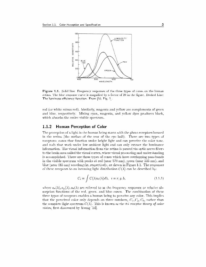
Figure 1.1. Solid line: Frequency responses of the three types of cones on the human
retina. The blue response curve is magni�ed by a factor of 20 in the �gure. Dashed Line:
The luminous eÆciency function. From [10, Fig. 1].
red (or white minus red). Similarly, magenta and yellow are complements of green
and blue, respectively. Mixing cyan, magenta, and yellow dyes produces black,
which absorbs the entire visible spectrum.
1.1.2 Human Perception of Color
The perception of a light in the human being starts with the photo receptors located
in the retina (the surface of the rear of the eye ball). There are two types of
receptors: cones that function under bright light and can perceive the color tone,
and rods that work under low ambient light and can only extract the luminance
information. The visual information from the retina is passed via optic nerve �bers
to the brain area called the visual cortex, where visual processing and understanding
is accomplished. There are three types of cones which have overlapping pass-bands
in the visible spectrum with peaks at red (near 570 nm), green (near 535 nm), and
blue (near 445 nm) wavelengths, respectively, as shown in Figure 1.1. The responses
of these receptors to an incoming light distribution C(�) can be described by:
Ci =
ZC(�)ai(�)d�; i = r; g; b; (1.1.1)
where ar(�); ag(�); ab(�) are referred to as the frequency responses or relative ab-
sorption functions of the red, green, and blue cones. The combination of these
three types of receptors enables a human being to perceive any color. This implies
that the perceived color only depends on three numbers, Cr; Cg ; Cb, rather than
the complete light spectrum C(�). This is known as the tri-receptor theory of color
vision, �rst discovered by Young [14].
4 Video Formation, Perception, and Representation Chapter 1
There are two attributes that describe the color sensation of a human being:
luminance and chrominance. The term luminance refers to the perceived brightness
of the light, which is proportional to the total energy in the visible band. The term
chrominance describes the perceived color tone of a light, which depends on the
wavelength composition of the light. Chrominance is in turn characterized by two
attributes: hue and saturation. Hue speci�es the color tone, which depends on
the peak wavelength of the light, while saturation describes how pure the color is,
which depends on the spread or bandwidth of the light spectrum. In this book, we
use the word color to refer to both the luminance and chrominance attributes of a
light, although it is customary to use the word color to refer to the chrominance
aspect of a light only.
Experiments have shown that there exists a secondary processing stage in the
human visual system (HVS), which converts the three color values obtained by the
cones into one value that is proportional to the luminance and two other values that
are responsible for the perception of chrominance. This is known as the opponent
color model of the HVS [3, 9]. It has been found that the same amount of energy
produces di�erent sensations of the brightness at di�erent wavelengths, and this
wavelength-dependent variation of the brightness sensation is characterized by a
relative luminous eÆciency function, ay(�), which is also shown (in dashed line)
in Fig. 1.1. It is essentially the sum of the frequency responses of all three types
of cones. We can see that the green wavelength contributes most to the perceived
brightness, the red wavelength the second, and the blue the least. The luminance
(often denoted by Y) is related to the incoming light spectrum by:
Y =
ZC(�)ay(�)d�: (1.1.2)
In the above equations, we have neglected the time and space variables, since we
are only concerned with the perceived color or luminance at a �xed spatial and
temporal location. We also neglected the scaling factor commonly associated with
each equation, which depends on the desired unit for describing the color intensities
and luminance.
1.1.3 The Trichromatic Theory of Color Mixture
A very important �nding in color physics is that most colors can be produced by
mixing three properly chosen primary colors. This is known as the trichromatic
theory of color mixture, �rst demonstrated by Maxwell in 1855 [9, 13]. Let Ck ; k =1; 2; 3 represent the colors of three primary color sources, and C a given color. Then
the theory essentially says
C =X
k=1;2;3
TkCk; (1.1.3)
where Tk's are the amounts of the three primary colors required to match color
C. The Tk's are known as tristimulus values. In general, some of the Tk's can be
Section 1.1. Color Perception and Speci�cation 5
negative. Assuming only T1 is negative, this means that one cannot match color
C by mixing C1; C2; C3, but one can match color C + jT1jC1 with T2C2 + T3C3:In practice, the primary colors should be chosen so that most natural colors can
be reproduced using positive combinations of primary colors. The most popular
primary set for the illuminating light source contains red, green, and blue colors,
known as the RGB primary. The most common primary set for the re ecting light
source contains cyan, magenta, and yellow, known as the CMY primary. In fact,
RGB and CMY primary sets are complement of each other, in that mixing two
colors in one set will produce one color in the other set. For example, mixing red
with green will yield yellow. This complementary information is best illustrated by
a color wheel, which can be found in many image processing books, e.g., [9, 4].
For a chosen primary set, one way to determine tristimulus values of any color
is by �rst determining the color matching functions, mi(�), for primary colors, Ci,
i=1,2,3. These functions describe the tristimulus values of a spectral color with
wavelength �, for various � in the entire visible band, and can be determined by
visual experiments with controlled viewing conditions. Then the tristimulus values
for any color with a spectrum C(�) can be obtained by [9]:
Ti =
ZC(�)mi(�)d�; i = 1; 2; 3: (1.1.4)
To produce all visible colors with positive mixing, the matching functions associated
with the primary colors must be positive.
The above theory forms the basis for color capture and display. To record the
color of an incoming light, a camera needs to have three sensors that have frequency
responses similar to the color matching functions of a chosen primary set. This can
be accomplished by optical or electronic �lters with the desired frequency responses.
Similarly, to display a color picture, the display device needs to emit three optical
beams of the chosen primary colors with appropriate intensities, as speci�ed by
the tristimulus values. In practice, electronic beams that strike phosphors with
the red, green and blue colors are used. All present display systems use a RGB
primary, although the standard spectra speci�ed for the primary colors may be
slightly di�erent. Likewise, a color printer can produce di�erent colors by mixing
three dyes with the chosen primary colors in appropriate proportions. Most of
the color printers use the CMY primary. For a more vivid and wide-range color
rendition, some color printers use four primaries, by adding black (K) to the CMY
set. This is known as the CMYK primary, which can render the black color more
truthfully.
1.1.4 Color Speci�cation by Tristimulus Values
Tristimulus Values We have introduced the tristimulus representation of a color
in Sec. 1.1.3, which speci�es the proportions, i.e. the Tk's in Eq. (1.1.3), of the
three primary colors needed to create the desired color. In order to make the color
speci�cation independent of the absolute energy of the primary colors, these values
6 Video Formation, Perception, and Representation Chapter 1
should be normalized so that Tk = 1; k = 1; 2; 3 for a reference white color (equal
energy in all wavelengths) with a unit energy. When we use a RGB primary, the
tristimulus values are usually denoted by R;G; and B.
Chromaticity Values: The above tristimulus representation mixes the luminance
and chrominance attributes of a color. To measure only the chrominance informa-
tion (i.e. the hue and saturation) of a light, the chromaticity coordinate is de�ned
as:
tk =Tk
T1 + T2 + T3; k = 1; 2; 3: (1.1.5)
Since t1 + t2 + t3 = 1, two chromaticity values are suÆcient to specify the chromi-
nance of a color.
Obviously, the color value of an imaged point depends on the primary colors
used. To standardize color description and speci�cation, several standard primary
color systems have been speci�ed. For example, the CIE, 2 an international body
of color scientists, de�ned a CIE RGB primary system, which consists of colors at
700 (R0), 546.1 (G0), and 435.8 (B0) nm.
Color Coordinate Conversion One can convert the color values based on one set
of primaries to the color values for another set of primaries. Conversion of (R,G,B)
coordinate to the (C,M,Y) coordinate is, for example, often required for printing
color images stored in the (R,G,B) coordinate. Given the tristimulus representation
of one primary set in terms of another primary, one can determine the conversion
matrix between the two color coordinates. The principle of color conversion and
the derivation of the conversion matrix between two sets of color primaries can be
found in [9].
1.1.5 Color Speci�cation by Luminance and Chrominance At-
tributes
The RGB primary commonly used for color display mixes the luminance and chromi-
nance attributes of a light. In many applications, it is desirable to describe a color
in terms of its luminance and chrominance content separately, to enable more ef-
�cient processing and transmission of color signals. Towards this goal, various
three-component color coordinates have been developed, in which one component
re ects the luminance and the other two collectively characterize hue and satura-
tion. One such coordinate is the CIE XYZ primary, in which Y directly measures
the luminance intensity. The (X;Y; Z) values in this coordinate are related to the
(R;G;B) values in the CIE RGB coordinate by [9]:
24 XYZ
35 =
24 2:365 �0:515 0:005�0:897 1:426 �0:014�0:468 0:089 1:009
3524 RGB
35 : (1.1.6)
2CIE stands for Commission Internationale de L'Eclariage or, in English, International Com-
mission on Illumination.
Section 1.2. Video Capture and Display 7
In addition to separating the luminance and chrominance information, another
advantage of the CIE XYZ system is that almost all visible colors can be speci�ed
with non-negative tristimulus values, which is a very desirable feature. The problem
is that the X,Y,Z colors so de�ned are not realizable by actual color stimuli. As
such, the XYZ primary is not directly used for color production, rather it is mainly
introduced for de�ning other primaries and for numerical speci�cation of color. As
will be seen later, the color coordinates used for transmission of color TV signals,
such as YIQ and YUV, are all derived from the XYZ coordinate.
There are other color representations in which the hue and saturation of a color
are explicitly speci�ed, in addition to the luminance. One example is the HSI coor-
dinate, where H stands for hue, S for saturation, and I for intensity (equivalent to
luminance)3. Although this color coordinate clearly separates di�erent attributes of
a light, it is nonlinearly related to the tristimulus values and is diÆcult to compute.
The book by Gonzalez has a comprehensive coverage of various color coordinates
and their conversions [4].
1.2 Video Capture and Display
1.2.1 Principle of Color Video Imaging
Having explained what is light and how it is perceived and characterized, we are
now in a position to understand the meaning of a video signal. In short, a video
records the emitted and/or re ected light intensity, i.e. C(X; t; �) from the objects
in the scene that is observed by a viewing system (a human eye or a camera). In
general, this intensity changes both in time and space. Here, we assume that there
are some illuminating light sources in the scene. Otherwise, there will be no injected
nor re ected light and the image will be totally dark. When observed by a camera,
only those wavelengths to which the camera is sensitive are visible. Let the spectral
absorption function of the camera be denoted by ac(�), then the light intensity
distribution in the 3D world that is \visible" to the camera is:
� (X; t) =
Z1
0
C(X; t; �)ac(�)d�: (1.2.1)
The image function captured by the camera at any time t is the projection of
the light distribution in the 3D scene onto a 2D image plane. Let P(�) representthe camera projection operator so that the projected 2D position of the 3D point
X is given by x = P(X). Further more, let P�1(�) denote the inverse projection
operator, so that X = P�1(x) speci�es the 3D position associated with a 2D point
x: Then the projected image is related to the 3D image by
(P(X); t) = � (X; t) or (x; t) = � �P�1(x); t
�: (1.2.2)
The function (x; t) is what is known as a video signal. We can see that it describes
the radiant intensity at the 3D position X that is projected onto x in the image
3The HSI coordinate is also known as HSV, where V stands for \value" of the intensity.
8 Video Formation, Perception, and Representation Chapter 1
plane at time t. In general the video signal has a �nite spatial and temporal range.
The spatial range depends on the camera viewing area, while the temporal range
depends on the duration in which the video is captured. A point in the image plane
is called a pixel (meaning picture element) or simply pel.4 For most camera systems,
the projection operator P(�) can be approximated by a perspective projection. Thisis discussed in more detail in Sec. 5.1.
If the camera absorption function is the same as the relative luminous eÆciency
function of the human being, i.e. ac(�) = ay(�), then a luminance image is formed.
If the absorption function is non-zero over a narrow band, then a monochrome
(or monotone) image is formed. To perceive all visible colors, according to the
trichromatic color vision theory (see Sec. 1.1.2), three sensors are needed, each with
a frequency response similar to the color matching function for a selected primary
color. As described before, most color cameras use the red, green, and blue sensors
for color acquisition.
If the camera has only one luminance sensor, (x; t) is a scalar function that
represents the luminance of the projected light. In this book, we use the word
gray-scale to refer to such a video. The term black-and-white will be used strictly
to describe an image that has only two colors: black and white. On the other hand,
if the camera has three separate sensors, each tuned to a chosen primary color, the
signal is a vector function that contains three color values at every point. Instead
of specifying these color values directly, one can use other color coordinates (each
consists of three values) to characterize light, as explained in the previous section.
Note that for special purposes, one may use sensors that work in a frequency
range that is invisible to the human being. For example, in X-ray imaging, the
sensor is sensitive to the spectral range of the X-ray. On the other hand, an infra-
red camera is sensitive to the infra-red range, which can function at very low ambient
light. These cameras can \see" things that cannot be perceived by the human eye.
Yet another example is the range camera, in which the sensor emits a laser beam and
measures the time it takes for the beam to reach an object and then be re ected
back to the sensor. Because the round trip time is proportional to the distance
between the sensor and the object surface, the image intensity at any point in a
range image describes the distance or range of its corresponding 3D point from the
camera.
1.2.2 Video Cameras
All the analog cameras of today capture a video in a frame by frame manner with
a certain time spacing between the frames. Some cameras (e.g. TV cameras and
consumer video camcorders) acquire a frame by scanning consecutive lines with a
certain line spacing. Similarly, all the display devices present a video as a consecu-
tive set of frames, and with TV monitors, the scan lines are played back sequentially
as separate lines. Such capture and display mechanisms are designed to take advan-
4Strictly speaking the notion of pixel or pel is only de�ned in digital imagery, in which each
image or a frame in a video is represented by a �nite 2D array of pixels.
Section 1.2. Video Capture and Display 9
tage of the fact that the HVS cannot perceive very high frequency changes in time
and space. This property of the HVS will be discussed more extensively in Sec. 2.4.
There are basically two types of video imagers: (1) tube-based imagers such
as vidicons, plumbicons, or orthicons, and (2) solid-state sensors such as charge-
coupled devices (CCD). The lens of a camera focuses the image of a scene onto a
photosensitive surface of the imager of the camera, which converts optical signals
into electrical signals. The photosensitive surface of the tube imager is typically
scanned line by line (known as raster scan) with an electron beam or other electronic
methods, and the scanned lines in each frame are then converted into an electrical
signal representing variations of light intensity as variations in voltage. Di�erent
lines are therefore captured at slightly di�erent times in a continuous manner. With
progressive scan, the electronic beam scans every line continuously; while with
interlaced scan, the beam scans every other line in one half of the frame time (a
�eld) and then scans the other half of the lines. We will discuss raster scan in more
detail in Sec. 1.3. With a CCD camera, the photosensitive surface is comprised of a
2D array of sensors, each corresponding to one pixel, and the optical signal reaching
each sensor is converted to an electronic signal. The sensor values captured in each
frame time are �rst stored in a bu�er, which are then read-out sequentially one line
at a time to form a raster signal. Unlike the tube based cameras, all the read-out
values in the same frame are captured at the same time. With interlaced scan
camera, alternate lines are read-out in each �eld.
To capture color, there are usually three types of photosensitive surfaces or CCD
sensors, each with a frequency response that is determined by the color matching
function of the chosen primary color, as described previously in Sec. 1.1.3. To reduce
the cost, most consumer cameras use a single CCD chip for color imaging. This is
accomplished by dividing the sensor area for each pixel into three or four sub-areas,
each sensitive to a di�erent primary color. The three captured color signals can be
either converted to one luminance signal and two chrominance signal and sent out
as a component color video, or multiplexed into a composite signal. This subject is
explained further in Sec. 1.2.4.
Many cameras of today are CCD-based because they can be made much smaller
and lighter than the tube-based cameras, to acquire the same spatial resolution.
Advancement in CCD technology has made it possible to capture in a very small
chip size a very high resolution image array. For example, 1/3-in CCD's with 380 K
pixels are commonly found in consumer-use camcorders, whereas a 2/3-in CCD with
2 million pixels has been developed for HDTV. The tube-based cameras are more
bulky and costly, and are only used in special applications, such as those requiring
very high resolution or high sensitivity under low ambient light. In addition to the
circuitry for color imaging, most cameras also implement color coordinate conversion
(from RGB to luminance and chrominance) and compositing of luminance and
chrominance signals. For digital output, analog-to-digital (A/D) conversion is also
incorporated. Figure 1.2 shows the typical processings involved in a professional
video camera. The camera provides outputs in both digital and analog form, and in
the analog case, includes both component and composite formats. To improve the
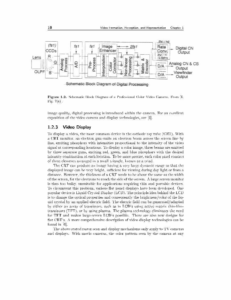
10 Video Formation, Perception, and Representation Chapter 1
Figure 1.2. Schematic Block Diagram of a Professional Color Video Camera. From [6,
Fig. 7(a)].
image quality, digital processing is introduced within the camera. For an excellent
exposition of the video camera and display technologies, see [6].
1.2.3 Video Display
To display a video, the most common device is the cathode ray tube (CRT). With
a CRT monitor, an electron gun emits an electron beam across the screen line by
line, exciting phosphors with intensities proportional to the intensity of the video
signal at corresponding locations. To display a color image, three beams are emitted
by three separate guns, exciting red, green, and blue phosphors with the desired
intensity combination at each location. To be more precise, each color pixel consists
of three elements arranged in a small triangle, known as a triad.
The CRT can produce an image having a very large dynamic range so that the
displayed image can be very bright, suÆcient for viewing during day light or from a
distance. However, the thickness of a CRT needs to be about the same as the width
of the screen, for the electrons to reach the side of the screen. A large screen monitor
is thus too bulky, unsuitable for applications requiring thin and portable devices.
To circumvent this problem, various at panel displays have been developed. One
popular device is Liquid Crystal Display (LCD). The principle idea behind the LCD
is to change the optical properties and consequently the brightness/color of the liq-
uid crystal by an applied electric �eld. The electric �eld can be generated/adapted
by either an array of transistors, such as in LCD's using active matrix thin-�lm-
transistors (TFT), or by using plasma. The plasma technology eliminates the need
for TFT and makes large-screen LCD's possible. There are also new designs for
at CRT's. A more comprehensive description of video display technologies can be
found in [6].
The above stated raster scan and display mechanisms only apply to TV cameras
and displays. With movie cameras, the color pattern seen by the camera at any
Section 1.2. Video Capture and Display 11
frame instant is completely recorded on the �lm. For display, consecutive recorded
frames are played back using an analog optical projection system.
1.2.4 Composite vs. Component Video
Ideally, a color video should be speci�ed by three functions or signals, each de-
scribing one color component, in either a tristimulus color representation, or a
luminance-chrominance representation. A video in this format is known as com-
ponent video. Mainly for historical reasons, various composite video formats also
exist, wherein the three color signals are multiplexed into a single signal. These
composite formats were invented when the color TV system was �rst developed and
there was a need to transmit the color TV signal in a way so that a black-and-
white TV set can extract from it the luminance component. The construction of
a composite signal relies on the property that the chrominance signals have a sig-
ni�cantly smaller bandwidth than the luminance component. By modulating each
chrominance component to a frequency that is at the high end of the luminance
component, and adding the resulting modulated chrominance signals and the orig-
inal luminance signal together, one creates a composite signal that contains both
luminance and chrominance information. To display a composite video signal on a
color monitor, a �lter is used to separate the modulated chrominance signals and the
luminance signal. The resulting luminance and chrominance components are then
converted to red, green, and blue color components. With a gray-scale monitor, the
luminance signal alone is extracted and displayed directly.
All present analog TV systems transmit color TV signals in a composite format.
The composite format is also used for video storage on some analog tapes (such
as the VHS tape). In addition to being compatible with a gray-scale signal, the
composite format eliminates the need for synchronizing di�erent color components
when processing a color video. A composite signal also has a bandwidth that is
signi�cantly lower than the sum of the bandwidth of three component signals, and
therefore can be transmitted or stored more eÆciently. These bene�ts are however
achieved at the expense of video quality: there often exist noticeable artifacts caused
by cross-talks between color and luminance components.
As a compromise between the data rate and video quality, S-video was invented,
which consists of two components, the luminance component and a single chromi-
nance component which is the multiplex of two original chrominance signals. Many
advanced consumer level video cameras and displays enable recording/display of
video in S-video format. Component format is used only in professional video
equipment.
1.2.5 Gamma Correction
We have said that the video frames captured by a camera re ect the color values of
the imaged scene. In reality, the output signals from most cameras are not linearly
12 Video Formation, Perception, and Representation Chapter 1
related to the actual color values, rather in a non- linear form:5
vc = B� cc ; (1.2.3)
where Bc represents the actual light brightness, and vc the camera output voltage.The value of c range from 1.0 for most CCD cameras to 1.7 for a vidicon camera
[7]. Similarly, most of the display devices also su�er from such a non-linear relation
between the input voltage value vd and the displayed color intensity Bd, i.e.
Bd = vd d : (1.2.4)
The CRT displays typically have a d of 2.2 to 2.5 [7]. In order to present true colors,one has to apply an inverse power function on the camera output. Similarly, before
sending real image values for display, one needs to pre-compensate the gamma e�ect
of the display device. These processes are known as gamma correction.
In TV broadcasting, ideally, at the TV broadcaster side, the RGB values cap-
tured by the TV cameras should �rst be corrected based on the camera gamma and
then converted to the color coordinates used for transmission (YIQ for NTSC, and
YUV for PAL and SECAM). At the receiver side, the received YIQ or YUV values
should �rst be converted to the RGB values, and then compensated for the monitor
gamma values. In reality, however, in order to reduce the processing to be done
in the millions of receivers, the broadcast video signals are pre-gamma corrected in
the RGB domain. Let vc represent the R, G, or B signal captured by the camera,
the gamma corrected signal for display, vd, is obtained by
vd = v c= dc : (1.2.5)
In most of the TV systems, a ratio of c= d = 2:2 is used. This is based on the
assumption that a CCD camera with c = 1 and a CRT display with d = 2:2 are
used [7]. These gamma corrected values are converted to the YIQ or YUV values for
transmission. The receiver simply applies a color coordinate conversion to obtain the
RGB values for display. Notice that this process applies display gamma correction
before the conversion to the YIQ/YUV domain, which is not strictly correct. But
the distortion is insigni�cant and not noticeable by average viewers [7].
1.3 Analog Video Raster
As already described, the analog TV systems of today use raster scan for video
capture and display. As this is the most popular analog video format, in this
section, we describe the mechanism of raster scan in more detail, including both
progressive and interlaced scan. As an example, we also explain the video formats
used in various analog TV systems.
5A more precise relation is Bc = cv cc +B0; where c is a gain factor, and B0 is the cut-o� level
of light intensity. If we assume that the output voltage value is properly shifted and scaled, then
the presented equation is valid.
Section 1.3. Analog Video Raster 13
Field 1 Field 2
Progressive Frame Interlaced Frame
(a) (b)
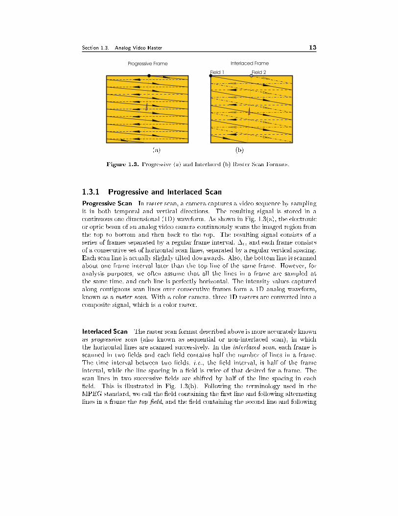
Figure 1.3. Progressive (a) and Interlaced (b) Raster Scan Formats.
1.3.1 Progressive and Interlaced Scan
Progressive Scan In raster scan, a camera captures a video sequence by sampling
it in both temporal and vertical directions. The resulting signal is stored in a
continuous one dimensional (1D) waveform. As shown in Fig. 1.3(a), the electronic
or optic beam of an analog video camera continuously scans the imaged region from
the top to bottom and then back to the top. The resulting signal consists of a
series of frames separated by a regular frame interval, �t, and each frame consists
of a consecutive set of horizontal scan lines, separated by a regular vertical spacing.
Each scan line is actually slightly tilted downwards. Also, the bottom line is scanned
about one frame interval later than the top line of the same frame. However, for
analysis purposes, we often assume that all the lines in a frame are sampled at
the same time, and each line is perfectly horizontal. The intensity values captured
along contiguous scan lines over consecutive frames form a 1D analog waveform,
known as a raster scan. With a color camera, three 1D rasters are converted into a
composite signal, which is a color raster.
Interlaced Scan The raster scan format described above is more accurately known
as progressive scan (also known as sequential or non-interlaced scan), in which
the horizontal lines are scanned successively. In the interlaced scan, each frame is
scanned in two �elds and each �eld contains half the number of lines in a frame.
The time interval between two �elds, i.e., the �eld interval, is half of the frame
interval, while the line spacing in a �eld is twice of that desired for a frame. The
scan lines in two successive �elds are shifted by half of the line spacing in each
�eld. This is illustrated in Fig. 1.3(b). Following the terminology used in the
MPEG standard, we call the �eld containing the �rst line and following alternating
lines in a frame the top �eld, and the �eld containing the second line and following
14 Video Formation, Perception, and Representation Chapter 1
alternating lines the bottom �eld. 6 In certain systems, the top �eld is sampled
�rst, while in other systems, the bottom �eld is sampled �rst. It is important to
remember that two adjacent lines in a frame are separated in time by the �eld
interval. This fact leads to the infamous zig-zag artifacts in an interlaced video
that contains fast moving objects with vertical edges. The motivation for using
the interlaced scan is to trade o� the vertical resolution for an enhanced temporal
resolution, given the total number of lines that can be recorded within a given time.
A more thorough comparison of the progressive and interlaced scans in terms of
their sampling eÆciency is given later in Sec. 3.3.2.
The interlaced scan introduced above should be called 2:1 interlace more pre-
cisely. In general, one can divide a frame into K � 2 �elds, each separated in time
by �t=K: This is known as K:1 interlace and K is called interlace order. In a digital
video where each line is represented by discrete samples, the samples on the same
line may also appear in di�erent �elds. For example, the samples in a frame may be
divided into two �elds using a checker-board pattern. The most general de�nition
of the interlace order is the ratio of the number of samples in a frame to the number
of samples in each �eld.
1.3.2 Characterization of a Video Raster
A raster is described by two basic parameters: the frame rate (frames/second or fps
or Hz), denoted by fs;t; and the line number (lines/frame or lines/picture-height),
denoted by fs;y. These two parameters de�ne the temporal and vertical sampling
rates of a raster scan. From these parameters, one can derive another important
parameter, the line rate (lines/second), denoted by fl = fs;tfs;y:7 We can also
derive the temporal sampling interval or frame interval, �t = 1=fs;t, the vertical
sampling interval or line spacing, �y = picture-height=fs;y, and the line interval,
Tl = 1=fl = �t=fs;y, which is the time used to scan one line. Note that the line
interval Tl includes the time for the sensor to move from the end of a line to the
beginning of the next line, which is known as the horizontal retrace time or just
horizontal retrace, to be denoted by Th. The actual scanning time for a line is
T 0l = Tl � Th: Similarly, the frame interval �t includes the time for the sensor to
move from the end of the bottom line in a frame to the beginning of the top line
of the next frame, which is called vertical retrace time or just vertical retrace, to be
denoted by Tv: The number of lines that is actually scanned in a frame time, known
as the active lines, is f 0s;y = (�t � Tv)=Tl = fs;y � Tv=Tl: Normally, Tv is chosen to
be an integer multiple of Tl:A typical waveform of an interlaced raster signal is shown in Fig. 1.4(a). Notice
that a portion of the signal during the horizontal and vertical retrace periods are
held at a constant level below the level corresponding to black. These are called
6A more conventional de�nition is to call the �eld that contains all even lines the even-�eld,
and the �eld containing all odd lines the odd-�eld. This de�nition depends on whether the �rst
line is numbered 0 or 1, and is therefore ambiguous.7The frame rate and line rate are also known as the vertical sweep frequency and the horizontal
sweep frequency, respectively.
Section 1.3. Analog Video Raster 15
(a)
Horizontal retrace
for first field
Vertical retrace
from first to second field
Vertical retrace
from second to third field
Blanking level
Black level
White level
(b)
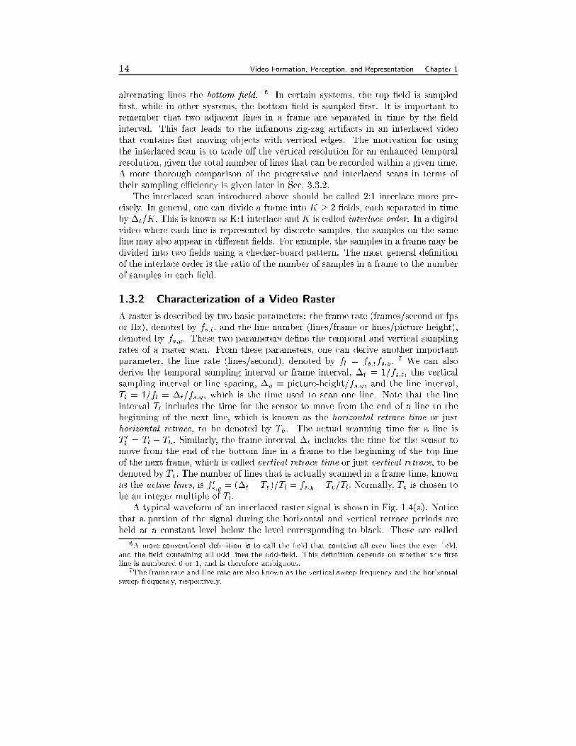
Figure 1.4. A Typical Interlaced Raster Scan: (a) Waveform, (b) Spectrum.
sync signals. The display devices start the retrace process upon detecting these
sync signals.
Figure 1.4(b) shows the spectrum of a typical raster signal. It can be seen that
the spectrum contains peaks at the line rate fl and its harmonics. This is because
adjacent scan lines are very similar so that the signal is nearly periodic with a
period of Tl: The width of each harmonic lobe is determined by the maximum
vertical frequency in a frame. The overall bandwidth of the signal is determined by
the maximum horizontal spatial frequency.
The frame rate is one of the most important parameters that determine the
quality of a video raster. For example, the TV industry uses an interlaced scan
with a frame rate of 25{30 Hz, with an e�ective temporal refresh rate of 50-60 Hz,
while the movie industry uses a frame rate of 24 Hz.8 On the other hand, in the
8To reduce the visibility of icker, a rotating blade is used to create an illusion of 72 frames/c.
16 Video Formation, Perception, and Representation Chapter 1
Luminance,
Chrominance,
Audio
Multiplexing
Modulation
De-
Modulation
De-
Multiplexing
YC1C2
--->
RGB
RGB
--->
YC1C2
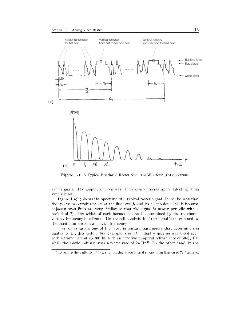
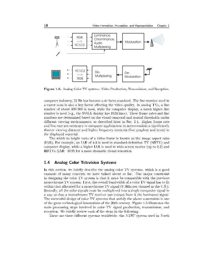
Figure 1.5. Analog Color TV systems: Video Production, Transmission, and Reception.
computer industry, 72 Hz has become a de facto standard. The line number used in
a raster scan is also a key factor a�ecting the video quality. In analog TVs, a line
number of about 500-600 is used, while for computer display, a much higher line
number is used (e.g., the SVGA display has 1024 lines). These frame rates and line
numbers are determined based on the visual temporal and spatial thresholds under
di�erent viewing environments, as described later in Sec. 2.4. Higher frame rate
and line rate are necessary in computer applications to accommodate a signi�cantly
shorter viewing distance and higher frequency contents (line graphics and texts) in
the displayed material.
The width to height ratio of a video frame is known as the image aspect ratio
(IAR). For example, an IAR of 4:3 is used in standard-de�nition TV (SDTV) and
computer display, while a higher IAR is used in wide-screen movies (up to 2.2) and
HDTVs (IAR=16:9) for a more dramatic visual sensation.
1.4 Analog Color Television Systems
In this section, we brie y describe the analog color TV systems, which is a good
example of many concepts we have talked about so far. One major constraint
in designing the color TV system is that it must be compatible with the previous
monochrome TV system. First, the overall bandwidth of a color TV signal has to �t
within that allocated for a monochrome TV signal (6 MHz per channel in the U.S.).
Secondly, all the color signals must be multiplexed into a single composite signal in
a way so that a monochrome TV receiver can extract from it the luminance signal.
The successful design of color TV systems that satisfy the above constraints is one
of the great technological innovations of the 20th century. Figure 1.5 illustrates the
main processing steps involved in color TV signal production, transmission, and
reception. We brie y review each of the steps in the following.
There are three di�erent systems worldwide: the NTSC system used in North
Section 1.4. Analog Color Television Systems 17
America as well as some other parts of Asia, including Japan and Taiwan; the
PAL system used in most of Western Europe and Asia including China, and the
Middle East countries; and the SECAM system used in the former Soviet Union,
Eastern Europe, France, as well as Middle East. We will compare these systems
in terms of their spatial and temporal resolution, the color coordinate, as well as
the multiplexing mechanism. The materials presented here are mainly from [9, 10].
More complete coverage on color TV systems can be found in [5, 1].
1.4.1 Spatial and Temporal Resolutions
All three color TV systems use the 2:1 interlaced scan mechanism described in
Sec. 1.3 for capturing as well as displaying video. The NTSC system uses a �eld
rate of 59.94 Hz, and a line number of 525 lines/frame. The PAL and SECAM
systems both use a �eld rate of 50 Hz and a line number of 625 lines/frame. These
frame rates are chosen to not to interfere with the standard electric power systems in
the involved countries. They also turned out to be a good choice in that they match
with the critical icker fusion frequency of the human visual system, as described
later in Sec. 2.4. All systems have an IAR of 4:3. The parameters of the NTSC,
PAL, and SECAM video signals are summarized in Table 1.1. For NTSC, the line
interval is Tl=1/(30*525)=63.5 �s. But the horizontal retrace takes Th=10 �s, sothat the actual time for scanning each line is T 0l=53.5 �s. The vertical retrace
between adjacent �elds takes Tv=1333 �s, which is equivalent to the time for 21
scan lines per �eld. Therefore, the number of active lines is 525-42=483/frame. The
actual vertical retrace only takes the time to scan 9 horizontal lines. The remaining
time (12 scan lines) are for broadcasters wishing to transmit additional data in the
TV signal (e.g., closed caption, teletext, etc.) 9
1.4.2 Color Coordinate
The color coordinate systems used in the three systems are di�erent. For video
capture and display, all three systems use a RGB primary, but with slightly di�erent
de�nitions of the spectra of individual primary colors. For transmission of the video
signal, in order to reduce the bandwidth requirement and to be compatible with
black and white TV systems, a luminance/chrominance coordinate is employed. In
the following, we describe the color coordinates used in these systems.
The color coordinates used in the NTSC, PAL and SECAM systems are all de-
rived from the YUV coordinate used in PAL, which in turn originates from the XYZ
coordinate. Based on the relation between the RGB primary and XYZ primary, one
can determine the Y value from the RGB value, which forms the luminance compo-
nent. The two chrominance values, U and V, are proportional to color di�erences,
B-Y and R-Y, respectively, scaled to have desired range. Speci�cally, the YUV
9The number of active lines cited in di�erent references vary from 480 to 495. This number is
calculated from the vertical blanking interval cited in [5].
18 Video Formation, Perception, and Representation Chapter 1
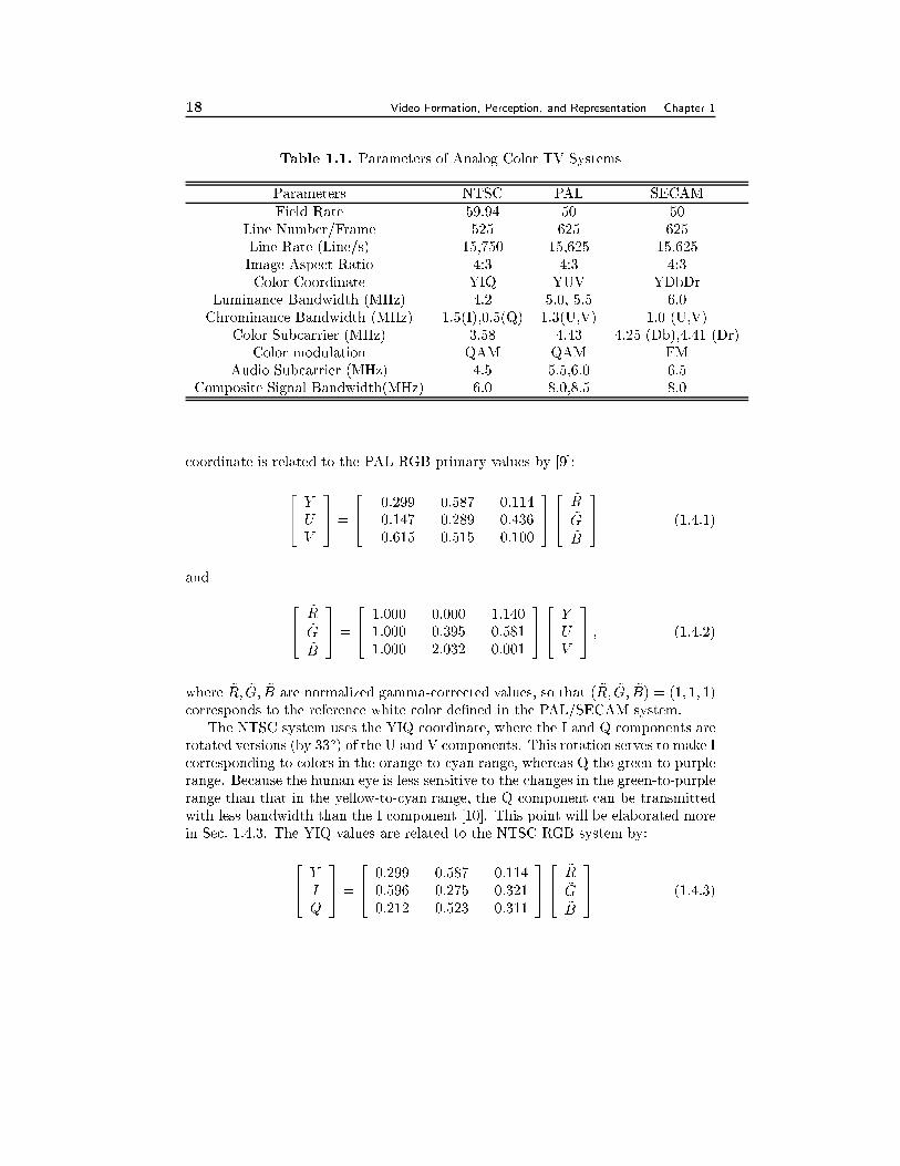
Table 1.1. Parameters of Analog Color TV Systems
Parameters NTSC PAL SECAM
Field Rate 59.94 50 50
Line Number/Frame 525 625 625
Line Rate (Line/s) 15,750 15,625 15,625
Image Aspect Ratio 4:3 4:3 4:3
Color Coordinate YIQ YUV YDbDr
Luminance Bandwidth (MHz) 4.2 5.0, 5.5 6.0
Chrominance Bandwidth (MHz) 1.5(I),0.5(Q) 1.3(U,V) 1.0 (U,V)
Color Subcarrier (MHz) 3.58 4.43 4.25 (Db),4.41 (Dr)
Color modulation QAM QAM FM
Audio Subcarrier (MHz) 4.5 5.5,6.0 6.5
Composite Signal Bandwidth(MHz) 6.0 8.0,8.5 8.0
coordinate is related to the PAL RGB primary values by [9]:
24 YUV
35 =
24 0:299 0:587 0:114�0:147 �0:289 0:4360:615 �0:515 �0:100
3524
~R~G~B
35 (1.4.1)
and
24
~R~G~B
35 =
24 1:000 0:000 1:140
1:000 �0:395 �0:5811:000 2:032 0:001
3524 YUV
35 ; (1.4.2)
where ~R; ~G; ~B are normalized gamma-corrected values, so that ( ~R; ~G; ~B) = (1; 1; 1)corresponds to the reference white color de�ned in the PAL/SECAM system.
The NTSC system uses the YIQ coordinate, where the I and Q components are
rotated versions (by 33o) of the U and V components. This rotation serves to make I
corresponding to colors in the orange-to-cyan range, whereas Q the green-to-purple
range. Because the human eye is less sensitive to the changes in the green-to-purple
range than that in the yellow-to-cyan range, the Q component can be transmitted
with less bandwidth than the I component [10]. This point will be elaborated more
in Sec. 1.4.3. The YIQ values are related to the NTSC RGB system by:
24 Y
IQ
35 =
24 0:299 0:587 0:114
0:596 �0:275 �0:3210:212 �0:523 0:311
3524
~R~G~B
35 (1.4.3)
Section 1.4. Analog Color Television Systems 19
and 24
~R~G~B
35 =
24 1:0 0:956 0:620
1:0 �0:272 �0:6471:0 �1:108 1:70
3524 Y
IQ
35 (1.4.4)
With the YIQ coordinate, tan�1(Q=I) approximates the hue, andpI2 +Q2=Y
re ects the saturation. In a NTSC composite video, the I and Q components are
multiplexed into one signal, so that the phase of the modulated signal is tan�1(Q=I),
whereas the magnitude equalspI2 +Q2=Y . Because transmission errors a�ect
the magnitude more than the phase, the hue information is better retained than
saturation in broadcast TV signal. This is desired, as the human eye is more
sensitive to the color hue. The name I and Q come from the fact that the I signal is
In-phase with the color modulation frequency, whereas the Q signal is in Quadrature
(i.e. 1/4 of the way around the circle or 90 degrees out of phase) with the modulation
frequency. The color multiplexing scheme is explained later in Sec. 1.4.4.
Note that because the RGB primary set and the reference white color used in
the NTSC system are di�erent from those in the PAL/SECAM system, the same
set of RGB values corresponds to slightly di�erent colors in these two systems.
The SECAM system uses the YDbDr coordinate, where the Db and Dr values
are related to the U and V values by [7]
Db = 3:059U; Dr = �2:169V: (1.4.5)
1.4.3 Signal Bandwidth
The bandwidth of a video raster can be estimated from its line rate. First of all,
the maximum vertical frequency results when the white and black lines alternate in
a raster frame, which is equal to f 0s;y=2 cycles/picture-height, where f 0s;y represent
the number of active lines. The maximum frequency that can be rendered properly
by a system is usually lower than this theoretical limit. The attenuation factor
is known as the Kell factor, denoted by K, which depends on the camera and
display aperture functions. Typical TV cameras have a Kell factor of K = 0:7: Themaximum vertical frequency that can be accommodated is related to the Kell factor
by
fv;max = Kf 0s;y=2 (cycles/picture-height): (1.4.6)
Assuming that the maximum horizontal frequency is identical to the vertical one
for the same spatial distance, then, fh;max = fv;maxIAR (cycles/picture-width).
Because each line is scanned in T 0l seconds, the maximum frequency in the 1D
raster signal is
fmax = fh;max=T0
l = IAR �Kf 0s;y=2T0
l Hz: (1.4.7)
For the NTSC video format, we have f 0s;y = 483; T 0l = 53:5 �s. Consequently, the
maximum frequency of the luminance component is 4.2 megacycles/second or 4.2
20 Video Formation, Perception, and Representation Chapter 1
MHz. Although the potential bandwidth of the chrominance signal could be just
as high, usually it is signi�cantly lower than the luminance signal. Furthermore,
the HVS has been found to have much lower threshold for observing changes in
chrominance. Because of the Typically, the two chrominance signals are bandlimited
to have much narrower bandwidth. As mentioned previously, the human eye is
more sensitive to spatial variations in the orange-to-cyan color range, represented
by the I component, than it is for the green-to-purple range, represented by the
Q component. Therefore, the I component is bandlimited to 1.5 MHz, and the
Q component to 0.5 MHz.10 Table 1.1 lists the signal bandwidth of di�erent TV
systems.
1.4.4 Multiplexing of Luminance, Chrominance, and Audio
In order to make the color TV signal compatible with the monochrome TV system,
all three analog TV systems use the composite video format, in which the three
color components as well as the audio component are multiplexed into one signal.
Here, we brie y describe the mechanism used by NTSC. First, the two chrominance
components I(t) and Q(t) are combined into a single signal C(t) using quadrature
amplitude modulation (QAM). The color sub-carrier frequency fc is chosen to be
an odd multiple of half of the line rate, fc = 455 fl2= 3.58 MHz. This is chosen
to satisfy the following criteria: i) It should be high enough where the luminance
component has very low energy; ii) It should be midway between two line rate har-
monics where the luminance component is strong; and iii) It should be suÆciently
far away from the audio sub-carrier, which is set at 4.5 MHz (286 fl), the same
as in the monochrome TV. Figure 1.6(a) shows how the harmonic peaks of the
luminance and chrominance signals interleave with each other. Finally, the audio
signal is frequency modulated (FM) using an audio sub-carrier frequency of fa =4.5MHz and added to the composite video signal, to form the �nal multiplexed signal.
Because the I component has a bandwidth of 1.5 MHz, the modulated chrominance
signal has a maximum frequency of up 5.08 MHz. In order to avoid the interference
with the audio signal, the chrominance signal is bandlimited in the upper sideband
to 0.6 MHz. Notice that the lower sideband of the I signal will run into the upper
part of the Y signal. For this reason, sometimes the I signal is bandlimited to 0.6
MHz on both sidebands. Finally, the entire composite signal, with a bandwidth of
about 4.75 MHz, is modulated onto a picture carrier frequency, fp, using vestigial
sideband modulation (VSB), so that the lower sideband only extends to 1.25 MHz
below fp and that the overall signal occupies 6 MHz. This process is the same as in
the monochrome TV system. The picture carrier fp depends on the broadcasting
channel. Figure 1.6(b) illustrates the spectral composition of the NTSC compos-
ite signal. The signal bandwidth and modulation methods in the three color TV
systems are summarized in Table 1.1.
At a television receiver, the composite signal �rst has to be demodulated to
the baseband, and then the audio and three components of the video signals must
10In [9], the bandwidth of I and Q are cited as 1.3 and 0.6 MHz, respectively.
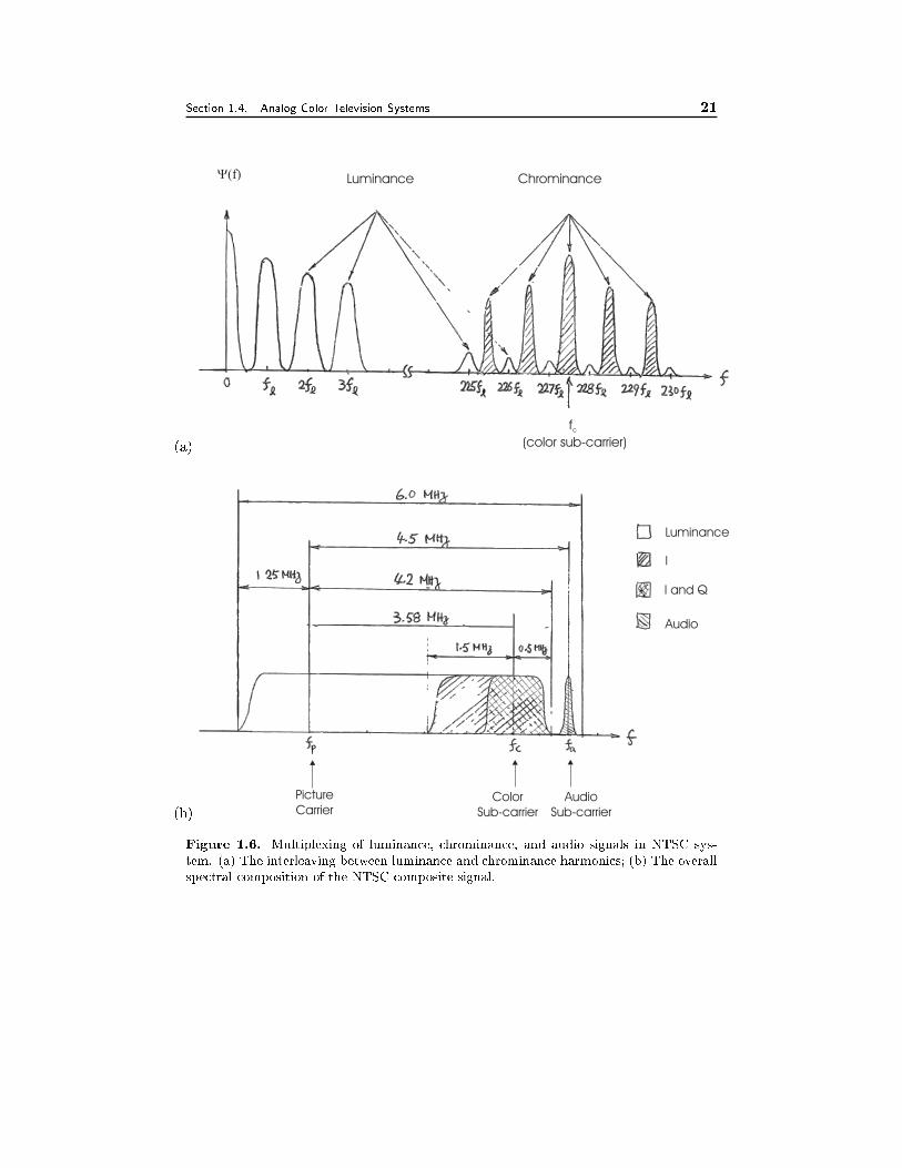
Section 1.4. Analog Color Television Systems 21
(a)
�� �f Luminance Chrominance
f
(color sub-carrier)c
(b)
Luminance
I
I and Q
Audio
Picture
CarrierColor
Sub-carrier
Audio
Sub-carrier
Figure 1.6. Multiplexing of luminance, chrominance, and audio signals in NTSC sys-
tem. (a) The interleaving between luminance and chrominance harmonics; (b) The overall
spectral composition of the NTSC composite signal.
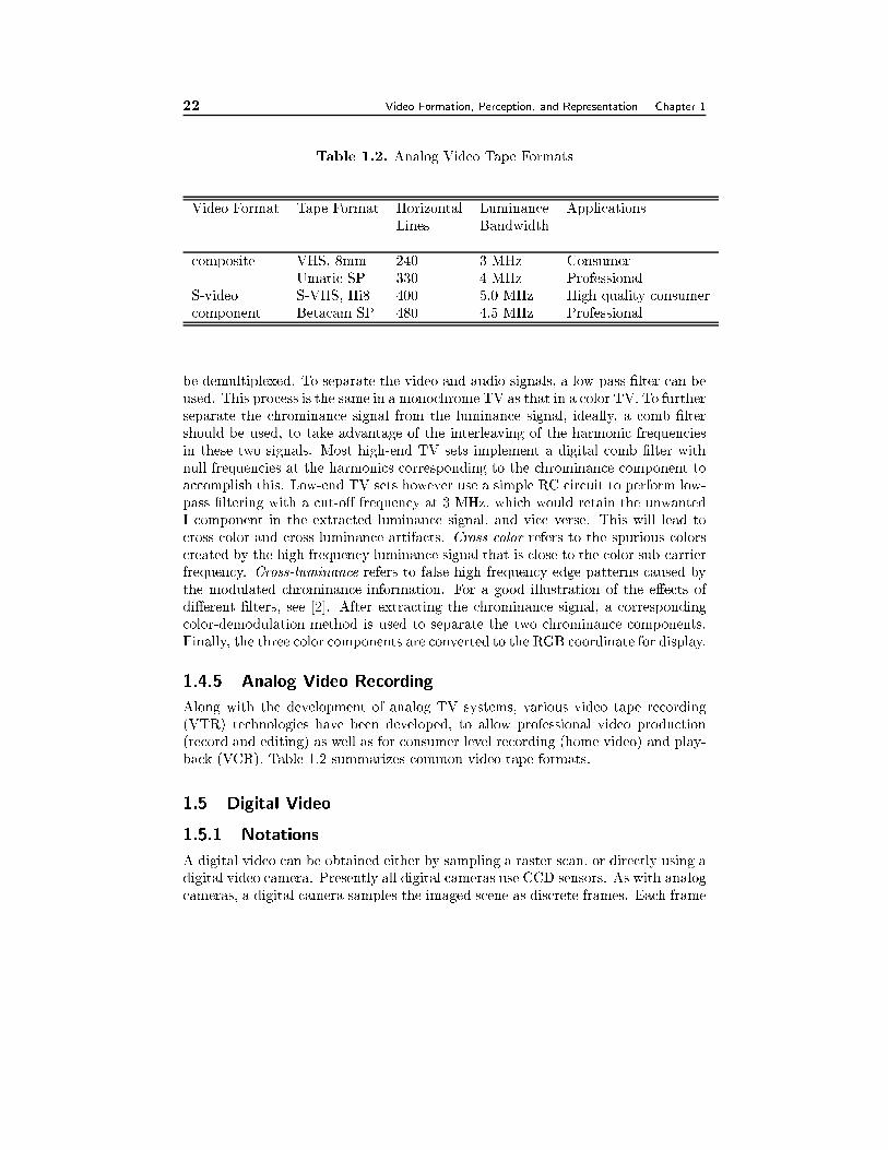
22 Video Formation, Perception, and Representation Chapter 1
Table 1.2. Analog Video Tape Formats
Video Format Tape Format Horizontal Luminance Applications
Lines Bandwidth
composite VHS, 8mm 240 3 MHz Consumer
Umatic SP 330 4 MHz Professional
S-video S-VHS, Hi8 400 5.0 MHz High quality consumer
component Betacam SP 480 4.5 MHz Professional
be demultiplexed. To separate the video and audio signals, a low-pass �lter can be
used. This process is the same in a monochrome TV as that in a color TV. To further
separate the chrominance signal from the luminance signal, ideally, a comb �lter
should be used, to take advantage of the interleaving of the harmonic frequencies
in these two signals. Most high-end TV sets implement a digital comb �lter with
null frequencies at the harmonics corresponding to the chrominance component to
accomplish this. Low-end TV sets however use a simple RC circuit to perform low-
pass �ltering with a cut-o� frequency at 3 MHz, which would retain the unwanted
I component in the extracted luminance signal, and vice verse. This will lead to
cross-color and cross-luminance artifacts. Cross-color refers to the spurious colors
created by the high frequency luminance signal that is close to the color sub-carrier
frequency. Cross-luminance refers to false high frequency edge patterns caused by
the modulated chrominance information. For a good illustration of the e�ects of
di�erent �lters, see [2]. After extracting the chrominance signal, a corresponding
color-demodulation method is used to separate the two chrominance components.
Finally, the three color components are converted to the RGB coordinate for display.
1.4.5 Analog Video Recording
Along with the development of analog TV systems, various video tape recording
(VTR) technologies have been developed, to allow professional video production
(record and editing) as well as for consumer level recording (home video) and play-
back (VCR). Table 1.2 summarizes common video tape formats.
1.5 Digital Video
1.5.1 Notations
A digital video can be obtained either by sampling a raster scan, or directly using a
digital video camera. Presently all digital cameras use CCD sensors. As with analog
cameras, a digital camera samples the imaged scene as discrete frames. Each frame
Section 1.5. Digital Video 23
comprises of output values from a CCD array, which is by nature discrete both
horizontal and vertically. A digital video is de�ned by the frame rate, fs;t, theline number, fs;y, as well as the number of samples per line, fs;x. From these, one
can �nd the temporal sampling interval or frame interval, �t = 1=fs;t, the verticalsampling interval �y = picture-height=fs;y, and the horizontal sampling interval
�x = picture-width=fs;x. In this book, we will use (m;n; k) to represent a digitalvideo, where integer indices m and n are the column and row indices, and k the
frame number. The actual spatial and temporal locations corresponding to the
integer indices are x = m�x; y = n�y, and t = k�t: For convenience, we use thenotation (x; y; t) to describe a video signal in a general context, which could be
either analog or digital. We will use (m;n; k) only when speci�cally addressing
digital video.
In addition to the above parameters, another important parameter of a digital
video is the number of bits used to represent a pixel value (luminance only or three
color values), to be denoted by Nb. Conventionally, the luminance or each of the
three color values is speci�ed with 8 bits or 256 levels. Therefore, Nb = 8 for
a monochrome video, while Nb = 24 for a color video. The data rate, R, of adigital video is determined by R = fs;tfs;xfs;yNb, with a unit of bits/second (bps).
Usually it is measured in kilobits/second (Kbps) or megabits/second (Mbps). In
general, the spatial and temporal sampling rates can be di�erent for the luminance
and chrominance components of a digital video. In this case, Nb should re ect the
equivalent number of bits used for each pixel in the luminance sampling resolution.
For example, if the horizontal and vertical sampling rates for each chrominance
component are both half of that for the luminance, then there are two chrominance
samples for every four Y samples. If each sample is represented with 8 bits, the
equivalent number of bits per sample in the Y resolution is (4*8+2*8)/4=12 bits.
When displaying the digital video on a monitor, each pixel is rendered as a
rectangular region with a constant color that is speci�ed for this pixel. The ratio of
the width to the height of this rectangular area is known as the pixel aspect ratio
(PAR). It is related to the IAR of the display area and the image dimension by
PAR = IAR � fs;y=fs;x: (1.5.1)
For proper display of a digitized video, one must specify either PAR or IAR, along
with fs;x and fs;y. The display device should conform to the PAR speci�ed for
this video (or derived from the speci�ed IAR). Otherwise, the object shape will be
distorted. For example, a person will become fatter and shorter, if the display PAR
is larger than the PAR speci�ed for this video. In computer industry, a PAR of
1.0 is normally used. On the other hand, in the TV industry, non-square pixels are
used because of some historical reasons. The rationale behind this is explained in
Sec. 1.5.2.
24 Video Formation, Perception, and Representation Chapter 1
1.5.2 ITU-R BT.601 Digital Video
Spatial Resolution of the BT.601 Signal In an attempt to standardize the digital
formats used to represent di�erent analog TV video signals with a quality equivalent
to broadcast TV, the International Telecommunications Union - Radio Sector (ITU-
R) developed the BT.601 recommendation [8]. The standard speci�es digital video
formats with both 4:3 and 16:9 aspect ratios. Here, we only discuss the version with
aspect ratio 4:3.11 To convert a raster scan to a digital video, one just needs to
sample the 1D waveform. If a total number of fs;x samples are taken per line, the
equivalent sampling rate is fs = fs;xfs;yfs;t = fs;xfl samples/second. In the BT.601standard, the sampling rate fs is chosen to satisfy two constraints: i) the horizontalsampling resolution should match with the vertical sampling resolution as closely
as possible, i.e. let �x � �y ; and ii) the same sampling rate should be used for the
NTSC and PAL/SECAM systems, and it should be multiples of respective line rates
in these systems. The �rst criterion calls for fs;x � IAR �fs;y, or fs � IAR �f2s;yfs;t,which leads to fs � 11 and 13 MHz for the NTSC and PAL/SECAM system. A
number that is closest to both numbers and yet satis�es the second criterion is then
chosen, which is
fs = 858fl (NTSC) = 864fl(PAL=SECAM) = 13:5MHz: (1.5.2)
The numbers of pixels per line are fs;x = 858 for NTSC and 864 for PAL/SECAM.
These two formats are known as 525/60 and 625/50 signals, respectively, and are
illustrated in Fig. 1.7. The numbers of active lines are respectively f 0s;y = 480 and
576 in the 525 and 625 line systems, but the number of active pixels/line are the
same, both equal to f 0s;x = 720 pixels. The rest are samples obtained during the
horizontal and vertical retraces, which fall in the non-active area.
With the BT.601 signal, the pixel width to height ratio is not one, i.e. the
physical area associated with a pixel is not a square. Speci�cally, PAR = �x=�y =
IAR � f 0s;y=f0
s;x = 8=9 for 525/60 and 16/15 for 625/50 signals. To display a BT.601
signal, the display device must has a proper PAR, otherwise the image will be
distorted. For example, when displayed on a computer screen which has a PAR
of 1, a 525/60 signal will appear stretched horizontally, while a 625/50 signal will
appear stretched vertically. Ideally, one should resample the original signal so that
f 0s;x = IAR � f 0s;y. For example, the 525/60 and 625/50 signals should be resampled
to have 640 and 768 active pixels/line, respectively.
Color Coordinate and Chrominance Subsampling Along with the image resolu-
tion, the BT.601 recommendation also de�nes a digital color coordinate, known as
YCbCr. The Y, Cb, and Cr components are scaled and shifted versions of the analog
Y, U, and V components, where the scaling and shifting operations are introduced
so that the resulting components take value in the range of (0,255). For a more
detailed explanation on the design this color coordinate, the readers are referred
11The ITU-R was formerly known as International Radio Consultative Committee (CCIR) and
the 4:3 aspect ratio version of the BT.601 format was called the CCIR601 format.
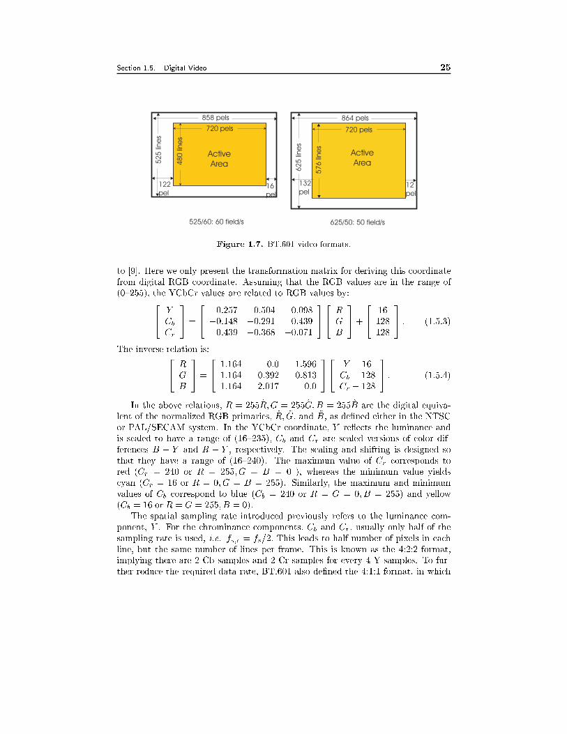
Section 1.5. Digital Video 25
48
0lin
es
52
5lin
es
122
pel16
pel
858 pels
720 pels
Active
Area
525/60: 60 field/s
57
6lin
es
62
5lin
es
864 pels
132
pel12
pel
720 pels
Active
Area
625/50: 50 field/s
Figure 1.7. BT.601 video formats.
to [9]. Here we only present the transformation matrix for deriving this coordinate
from digital RGB coordinate. Assuming that the RGB values are in the range of
(0{255), the YCbCr values are related to RGB values by:24 YCb
Cr
35 =
24 0:257 0:504 0:098�0:148 �0:291 0:4390:439 �0:368 �0:071
3524 RGB
35+
24 16
128
128
35 : (1.5.3)
The inverse relation is:24 RGB
35 =
24 1:164 0:0 1:596
1:164 �0:392 �0:8131:164 2:017 0:0
3524 Y � 16
Cb � 128
Cr � 128
35 : (1.5.4)
In the above relations, R = 255 ~R;G = 255 ~G;B = 255 ~B are the digital equiva-
lent of the normalized RGB primaries, ~R; ~G; and ~B, as de�ned either in the NTSC
or PAL/SECAM system. In the YCbCr coordinate, Y re ects the luminance and
is scaled to have a range of (16{235), Cb and Cr are scaled versions of color dif-
ferences B � Y and R � Y , respectively. The scaling and shifting is designed so
that they have a range of (16{240). The maximum value of Cr corresponds to
red (Cr = 240 or R = 255; G = B = 0 ), whereas the minimum value yields
cyan (Cr = 16 or R = 0; G = B = 255). Similarly, the maximum and minimum
values of Cb correspond to blue (Cb = 240 or R = G = 0; B = 255) and yellow
(Cb = 16 or R = G = 255; B = 0).
The spatial sampling rate introduced previously refers to the luminance com-
ponent, Y . For the chrominance components, Cb and Cr, usually only half of the
sampling rate is used, i.e. fs;c = fs=2: This leads to half number of pixels in each
line, but the same number of lines per frame. This is known as the 4:2:2 format,
implying there are 2 Cb samples and 2 Cr samples for every 4 Y samples. To fur-
ther reduce the required data rate, BT.601 also de�ned the 4:1:1 format, in which
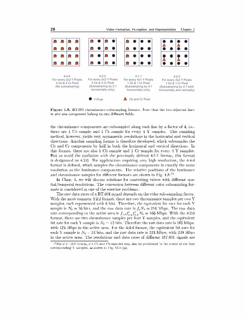
26 Video Formation, Perception, and Representation Chapter 1
4:2:0
For every 2x2 Y Pixels
1 Cb & 1 Cr Pixel
(Subsampling by 2:1 both
horizontally and vertically)
4:2:2
For every 2x2 Y Pixels
2 Cb & 2 Cr Pixel
(Subsampling by 2:1
horizontally only)
4:4:4
For every 2x2 Y Pixels
4 Cb & 4 Cr Pixel
(No subsampling)
Y Pixel Cb and Cr Pixel
4:1:1
For every 4x1 Y Pixels
1 Cb & 1 Cr Pixel
(Subsampling by 4:1
horizontally only)
Figure 1.8. BT.601 chrominance subsampling formats. Note that the two adjacent lines
in any one component belong to two di�erent �elds.
the chrominance components are subsampled along each line by a factor of 4, i.e.,
there are 1 Cb sample and 1 Cr sample for every 4 Y samples. This sampling
method, however, yields very asymmetric resolutions in the horizontal and vertical
directions. Another sampling format is therefore developed, which subsamples the
Cb and Cr components by half in both the horizontal and vertical directions. In
this format, there are also 1 Cb sample and 1 Cr sample for every 4 Y samples.
But to avoid the confusion with the previously de�ned 4:1:1 format, this format
is designated as 4:2:0. For applications requiring very high resolutions, the 4:4:4
format is de�ned, which samples the chrominance components in exactly the same
resolution as the luminance components. The relative positions of the luminance
and chrominance samples for di�erent formats are shown in Fig. 1.8.12
In Chap. 4, we will discuss solutions for converting videos with di�erent spa-
tial/temporal resolutions. The conversion between di�erent color subsampling for-
mats is considered in one of the exercise problems.
The raw data rates of a BT.601 signal depends on the color sub-sampling factor.
With the most common 4:2:2 format, there are two chrominance samples per two Y
samples, each represented with 8 bits. Therefore, the equivalent bit rate for each Y
sample is Nb = 16 bits, and the raw data rate is fsNb = 216 Mbps. The raw data
rate corresponding to the active area is fs;tf0
s;yf0
s;xNb = 166 Mbps. With the 4:2:0
format, there are two chrominance samples per four Y samples, and the equivalent
bit rate for each Y sample is Nb = 12 bits. Therefore the raw data rate is 162 Mbps,
with 124 Mbps in the active area. For the 4:4:4 format, the equivalent bit rate for
each Y sample is Nb = 24 bits, and the raw data rate is 324 Mbps, with 249 Mbps
in the active area. The resolutions and data rates of di�erent BT.601 signals are
12For the 4:2:0 format, the Cr and Cb samples may also be positioned in the center of the four
corresponding Y samples, as shown in Fig. 13.14(a).
Section 1.5. Digital Video 27
summarized in Table 1.3.
The BT.601 formats are used in high-quality digital video applications, with the
4:4:4 and 4:2:2 formats typically used for video production and editing, whereas 4:2:0
for video distribution, e.g., movies on digital video disks (DVD), video-on-demand
(VOD), etc. The MPEG2 13 video compression standard was primarily developed
for compression of BT.601 4:2:0 signals, although it can also handle videos in lower
or higher resolutions. A typical 4:2:0 signal with a raw active data rate of 124 Mbps
can be compressed down to about 4-8 Mbps. We will introduce the MPEG2 video
coding algorithm in Sec. 13.5.
1.5.3 Other Digital Video Formats and Applications
In addition to the BT.601 format, several other standard digital video formats have
been de�ned. Table 1.3 summarizes these video formats, along with their main
applications, compression methods, and compressed bit rates. The CIF (Com-
mon Intermediate Format) is speci�ed by International Telecommunications Union-
Telecommunications Sector (ITU-T), which has about half the resolution of BT.601
4:2:0 in both horizontal and vertical dimensions and is developed for video confer-
encing applications, and the QCIF, which is a quarter of CIF, used for video phone
type applications. Both are non-interlaced. The ITU-T H.261 coding standard was
developed to compress videos in either format to p�64 Kbps, with p = 1; 2; : : : ; 30,for transport over ISDN (integrated service digital network) lines, which only allow
transmission rates in multiples of 64 Kbps. Typically, a CIF signal with a raw
data rate of 37.3 Mbps can be compressed down to about 128 to 384 Kbps, with
reasonable quality, while a QCIF signal with a raw data rate of 9.3 Mbps can be
compressed to 64-128 Kbps. A later standard, H.263, can achieve better quality
than H.261, at the same bit rate. For example, it is possible to compress a QCIF
picture to about 20 Kbps, while maintaining a quality similar or better than H.261
at 64 Kbps. This enables video phone over a 28.8 Kbps modem line.
In parallel with the e�ort of ITU-T, the ISO-MPEG also de�ned a series of digital
video formats. The SIF (Source Intermediate Format) is essentially a quarter size
of the active area in the BT.601 signal, and is about the same as CIF. This format
is targeted for video applications requiring medium quality, such as video games
and CD movies. As with BT.601, there are two SIF formats: one with a frame rate
of 30 Hz and a line number of 240, and another with a frame rate of 25 and line
number of 288, both have 352 pixels/line. There is also a corresponding set of SIF-I
format, which is 2:1 interlaced. The MPEG-1 algorithm can compress a typical SIF
video with a raw data rate of 30 Mbps to about 1.1 Mbps with a quality similar to
the resolutions seen on a VHS VCR, which is lower than broadcast television. The
rate of 1.1 Mbps enables the playback of digital movies on CD-ROM's, which have
an access rate of 1.5 Mbps. Distribution of MPEG1 movies on video CD's (VCD)
marked the entrance of digital video into the consumer market in the early 1990's.
13MPEG standards for Motion Picture Expert Group of the International Standard Organization
or ISO.
28 Video Formation, Perception, and Representation Chapter 1
MPEG2-based DVD's, which started in mid 90's, opened the era of high quality
digital video entertainment. MPEG2 technology is also the corner stone of the next
generation TV system, which will be fully digital, employing digital compression and
transmission technology. Table 1.3 lists the details of the video formats discussed
above, along with their main applications, compression methods, and compressed
bit rates. More on compression standards will be presented in Chap. 13.
The BT.601 format is the standard picture format for digital TV (DTV). To
further enhance the video quality, several HDTV formats have also been standard-
ized by the Society of Motion Picture and Television Engineers (SMPTE), which
are also listed in Table 1.3. A distinct feature of HDTV is its wider aspect ratio,
16:9 as opposed to 4:3 in SDTV. The picture resolution is doubled to tripled in
both horizontal and vertical dimensions. Furthermore, progressive scan is used to
reduce the interlacing artifacts. A high pro�le has been developed in the MPEG2
video compression standard for compressing HDTV video. Typically it can reduce
the data rate to about 20 Mbps while retaining the very high quality required. This
video bit rate is chosen so that the combined bit stream with audio, when trans-
mitted using digital modulation techniques, can still �t into a 6 MHz terrestrial
channel, which is the assigned channel bandwidth for HDTV broadcast in the U.S.
1.5.4 Digital Video Recording
To store video in digital formats, various digital video tape recorder (DVTR) for-
mats have been developed, which di�er in the video format handled and technology
for error-correction-coding and storage density. Table 1.4 lists some standard and
proprietary tape formats. The D1-D5 formats store a video in its raw, uncom-
pressed formats, while others pre-compress the video. Only a conservative amount
of compression is employed so as not to degrade the video quality beyond that ac-
ceptable for the intended application. A good review of digital VTRs can be found
in [11]. A extensive coverage on the underlying physics of magnetic recording and
operation of DVTRs can be found in the book by Watkinson [12].
In addition to magnetic tape recorders, VCD and DVD are two video storage
devices using optical disks. By incorporating MPEG1 and MPEG2 compression
technologies, they can store SIF and BT.601 videos, respectively, with suÆcient
quality. At present, VCD and DVD are read-only, so that they are mainly used
for distribution of pre-recorded video, as opposed to as tools for recording video by
consumers.
Except video recording systems using magnetic tapes, hard-disk based systems,
such as TiVo and ReplayTV, are also on the horizon. These systems enable con-
sumers to record up to 30 hours of live TV programs onto hard-disks in MPEG-2
compressed formats, which can be viewed later with usual VCR features such as
fast forward, slow motion, etc. They also allow instant pause of a live program
that is being watched, by storing the live video from the time of the pause onto the
disk. As the price for hard-disks drops down continuously, hard-disk-based DVTR's
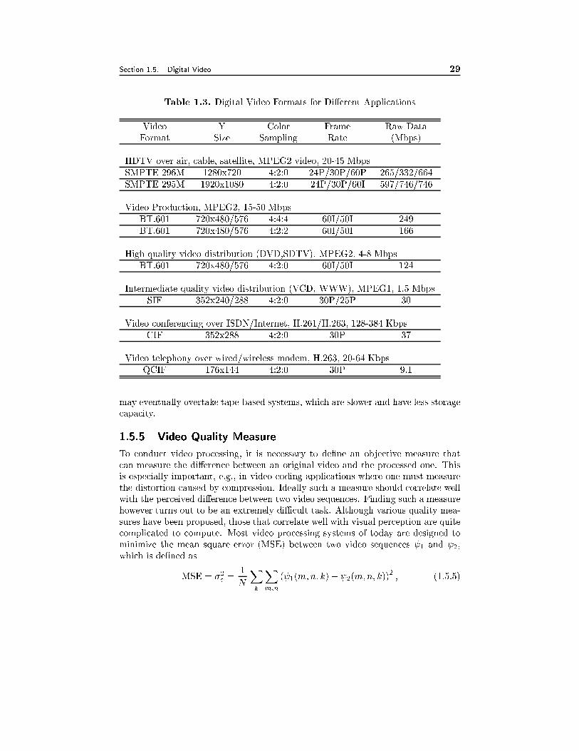
Section 1.5. Digital Video 29
Table 1.3. Digital Video Formats for Di�erent Applications
Video Y Color Frame Raw Data
Format Size Sampling Rate (Mbps)
HDTV over air, cable, satellite, MPEG2 video, 20-45 Mbps
SMPTE 296M 1280x720 4:2:0 24P/30P/60P 265/332/664
SMPTE 295M 1920x1080 4:2:0 24P/30P/60I 597/746/746
Video Production, MPEG2, 15-50 Mbps
BT.601 720x480/576 4:4:4 60I/50I 249
BT.601 720x480/576 4:2:2 60I/50I 166
High quality video distribution (DVD,SDTV), MPEG2, 4-8 Mbps
BT.601 720x480/576 4:2:0 60I/50I 124
Intermediate quality video distribution (VCD, WWW), MPEG1, 1.5 Mbps
SIF 352x240/288 4:2:0 30P/25P 30
Video conferencing over ISDN/Internet, H.261/H.263, 128-384 Kbps
CIF 352x288 4:2:0 30P 37
Video telephony over wired/wireless modem, H.263, 20-64 Kbps
QCIF 176x144 4:2:0 30P 9.1
may eventually overtake tape-based systems, which are slower and have less storage
capacity.
1.5.5 Video Quality Measure
To conduct video processing, it is necessary to de�ne an objective measure that
can measure the di�erence between an original video and the processed one. This
is especially important, e.g., in video coding applications where one must measure
the distortion caused by compression. Ideally such a measure should correlate well
with the perceived di�erence between two video sequences. Finding such a measure
however turns out to be an extremely diÆcult task. Although various quality mea-
sures have been proposed, those that correlate well with visual perception are quite
complicated to compute. Most video processing systems of today are designed to
minimize the mean square error (MSE) between two video sequences 1 and 2,which is de�ned as
MSE = �2e =1
N
Xk
Xm;n
( 1(m;n; k)� 2(m;n; k))2; (1.5.5)
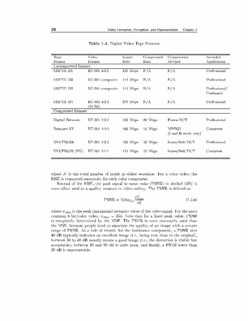
30 Video Formation, Perception, and Representation Chapter 1
Table 1.4. Digital Video Tape Formats
Tape Video Source Compressed Compression Intended
Format Format Rate Rate Method Application
Uncompressed formats
SMPTE D1 BT.601 4:2:2 216 Mbps N/A N/A Professional
SMPTE D2 BT.601 composite 114 Mbps N/A N/A Professional
SMPTE D3 BT.601 composite 114 Mbps N/A N/A Professional/
Consumer
SMPTE D5 BT.601 4:2:2 270 Mbps N/A N/A Professional
(10 bit)
Compressed formats
Digital Betacam BT.601 4:2:2 166 Mbps 80 Mbps Frame DCT Professional
Betacam SX BT.601 4:2:2 166 Mbps 18 Mbps MPEG2 Consumer
(I and B mode only)
DVCPRO50 BT.601 4:2:2 166 Mbps 50 Mbps frame/�eld DCT Professional
DVCPRO25 (DV) BT.601 4:1:1 124 Mbps 25 Mbps frame/�eld DCT Consumer
where N is the total number of pixels in either sequence. For a color video, the
MSE is computed separately for each color component.
Instead of the MSE, the peak signal to noise ratio (PSNR) in decibel (dB) is
more often used as a quality measure in video coding. The PSNR is de�ned as
PSNR = 10 log10
2max
�2e(1.5.6)
where max is the peak (maximum) intensity value of the video signal. For the most
common 8 bit/color video, max = 255: Note that for a �xed peak value, PSNR
is completely determined by the MSE. The PSNR is more commonly used than
the MSE, because people tend to associate the quality of an image with a certain
range of PSNR. As a rule of thumb, for the luminance component, a PSNR over
40 dB typically indicates an excellent image (i.e., being very close to the original),
between 30 to 40 dB usually means a good image (i.e., the distortion is visible but
acceptable), between 20 and 30 dB is quite poor, and �nally, a PSNR lower than
20 dB is unacceptable.
Section 1.6. Summary 31
It is worth noting that to compute the PSNR between two sequences, it is
incorrect to calculate the PSNR between every two corresponding frames and then
taking the average of the PSNR values obtained over individual frames. Rather
one should compute the MSE between corresponding frames, average the resulting
MSE values over all frames, and �nally convert the MSE value to PSNR.
A measure that is sometimes used in place of the MSE, mainly for reduced
computation, is the mean absolute di�erence (MAD). This is de�ned as
MAD =1
N
Xk
Xm;n
j 1(m;n; k)� 2(m;n; k)j : (1.5.7)
For example, for motion estimation, the MAD is usually used to �nd the best
matching block in another frame for a given block in a current frame.
It is well known that MSE or PSNR does not correlate very well with visual
distortion between two imagery. But these measures have been used almost exclu-
sively as objective distortion measures in image/video coding, motion compensated
prediction, and image restoration, partly because of their mathematical tractability,
and partly because of the lack of better alternatives. Designing objective distortion
measures that are easy to compute and yet correlate well with visual distortion is
still an open research issue. In this book, we will mostly use MSE or PSNR as the
distortion measure.
1.6 Summary
Color Generation, Perception, and Speci�cation (Sec. 1.1)
� The color of a light depends on its spectral content. Any color can be created
by mixing three primary colors. The most common primary set includes red,
green, and blue colors.
� The human eye perceives color by having receptors (cones) in the retina that
are tuned to red, green, and blue wavelengths. The color sentation can be
described by three attributes: luminance (i.e., brightness), hue (color tone),
and saturation (color purity). The human eye is most sensitive to luminance,
then to hue, and �nally to saturation.
� A color can be speci�ed by three numbers: either those corresponding to
the contributions of the three primary colors (i.e., tristimulus values), or a
luminance value and two chrominance values.
Analog Video (Sec. 1.3)
� Analog videos used in broadcasting TV, video camcorder, etc., video display,
are stored in a raster scan format. The visual quality and bandwidth of a
raster scan depends on its frame rate and line number.
32 Video Formation, Perception, and Representation Chapter 1
� Interlaced scan is a mechanism to trade o� vertical resolution for enhanced
temporal resolution. But it also leads to interlacing artifacts.
Analog Color TV Systems (Sec. 1.4)
� There are three analog color TV systems world wide: NTSC, PAL, and SE-
CAM. They all use 2:1 interlace, but di�er in frame rate, line number, color
coordinate, and luminance and chrominance multiplexing.
� In color TV systems, the luminance and two chrominance components as well
as the associated audio signal are multiplexed into a composite signal, us-
ing modulation (frequency shifting) techniques. The multiplexing methods
are designed so that the color TV system is downward compatible with the
monochrome TV system. Furthermore, the modulation frequencies for indi-
vidual components are chosen to minimize the interference among them.
Digital Video (Sec. 1.5)
� BT.601 is a digital video format, resulting from sampling the analog color TV
signals. The sampling rate is chosen so that the horizontal sampling rate is
similar to the vertical sampling rate, and that the data rates for NTSC and
PAL/SECAM systems are the same.
� The chrominance components can be sampled at a lower rate than the lumi-
nance component. There are di�erent color subsampling formats de�ned in
BT.601.
� Compression is necessary to reduce the raw data rate of a digital video to
reduce the storage/transmission cost. Di�erent video compression standards
have been developed for videos intended for di�erent applications.
1.7 Problems
1.1 Describe the mechanism by which the human being perceives color.
1.2 What is the perceived color if you have a light that has approximately the
same energy at frequencies corresponding to red, green, and blue, and are
zero at other frequencies ? What about red and green frequencies only ?
1.3 What is the perceived color if you mix red, green, and blue dyes in equal
proportion ? What about red and green dyes only ?
1.4 For the following colors in the RGB coordinate, determine their values in the
YIQ and YUV coordinates, respectively.
(a) (1,1,1); (b) (0,1,0); (c) (1,1,0); (d) (0, 1,1).
Section 1.8. Bibliography 33
1.5 For the following colors in the digital RGB coordinate, determine their values
in the YCbCr coordinate.
(a) (255,255, 255); (b) (0, 255, 0); (c) (255,255,0); (d) (0, 255, 255).
1.6 In Sec. 1.5.2, we say that the maximum value of Cr corresponds to red, whereas
the minimum value yields cyan . Similarly, the maximum and minimum values
of Cb correspond to blue and yellow, respectively. Verify these statements
using the YCbCr to RGB coordinate transformation.
1.7 In Fig. 1.4, we show the spectrum of a typical raster signal. Why is the
spectrum of the video signal nearly periodic? What does the width of harmonic
lobes depend on?
1.8 What are the pros and cons of progressive vs. interlaced scans? For the same
line number per frame, what is the relation between the maximum temporal
frequency that a progressive raster can have and that of an interlaced raster
which divides each frame into two �elds? What about the relation between
the maximum vertical frequencies?
1.9 In Sec. 1.4.3, we estimated the bandwidth of the NTSC signal based on its
scan parameters. Following the same approach, estimate the bandwidth of
the PAL and SECAM signals.
1.10 Describe the process for forming a composite color video signal. How should
you select the color sub-carrier frequency and audio sub-carrier frequency ?
1.11 What are the pros and cons of using component vs. composite format?
1.12 Project: Using an oscilloscope to i) draw the waveform, and ii) measure the
spectrum of a composite video signal output from a TV set or a camcorder.
1.13 Project: Digitize a composite video signal using an A/D converter, and using
Matlab to determine the spectrum. Also perform �ltering to separate the
luminance, chrominance and audio signals.
1.8 Bibliography
[1] K. B. Benson, editor. Television Engineering Handbook. McGraw Hill, 1992.
Revised by J.C.Whitaker.
[2] J. F. Blinn. NTSC: nice technology, super color. IEEE Computer Graphics and
Applications Magazine, pages 17{23, Mar. 1993.
[3] R. M. Boynton. Human Color Vision. Holt, Rinhart, Winston, New York, 1979.
[4] R. G. Gonzalez and R. E. Woods. Digital Image Processing. Addison{Wesley,
2nd edition, 1992.
34 Video Formation, Perception, and Representation Chapter 1
[5] B. Grob and C. E. Herndon. Basic Television and Video Systems. Glencoe
McGraw Hill, 6th edition, 1999.
[6] Y. Hashimoto, M. Yamamoto, and T. Asaida. Cameras and display systems.
Proc. of IEEE, pages 1032{1043, July 1995.
[7] B. G. Haskell, A. Puri, and A. N. Netravali. Digital Video: An Introduction to
MPEG-2. Chapman & Hall, New York, 1997.
[8] ITU-R. BT.601-5: Studio encoding parameters of digital television for standard
4:3 and wide-screen 16:9 aspect ratios, 1998. (Formerly CCIR 601).
[9] A. N. Netravali and B. G. Haskell. Digital Pictures - Representation, Compres-
sion and Standards. Plenum Press, 2nd edition, 1995.
[10] D. H. Pritchard. US color television fundamentals. IEEE Trans. Consum.
Electron., CE-23:467{78, 1977.
[11] M. Umemoto, Y. Eto, and T. Fukinuki. Digital video recording. Proc. of IEEE,
pages 1044{1054, July 1995.
[12] J. Watkinson. The Art of Digital Video. Focal Press, Oxford, 2nd edition,
1994.
[13] G. Wyszecki and W. S. Stiles. Color Science. John Wiley, New York, 1967.
[14] T. Young. On the theory of light and colors. Philosophical Transactions of the
Royal Society of London, 92:20{71, 1802.
Chapter 2
FOURIER ANALYSIS OF
VIDEO SIGNALS AND
PROPERTIES OF THE
HUMAN VISUAL SYSTEM
Fourier analysis is an important tool for signal analysis. We assume that the reader
is familiar with Fourier transforms for one- and two-dimensional (1D and 2D) spaces
as well as signal processing tools using such transforms. In this chapter, we �rst
extend these results to K-dimensions (K-D), where K can be any positive integer.
We then focus on their applications for video signals, which are three-dimensional
(3D). We will explore the meaning of spatial and temporal frequencies, and their
inter-relationship. Finally, we discuss visual sensitivity to di�erent frequency com-
ponents.
2.1 Multi-dimensional Continuous Space Signals and Systems
Most of the theorems and techniques for multi-dimensional signals and systems are
direct extensions of those developed for 1D and 2D signals and systems. In this
section, we introduce some important concepts and theorems for signal analysis in
the K-D real space, RK = f[x1; x2; : : : ; xK ]T jxk 2 R; k 2 Kg; where R is the set
of real numbers, and K = f1; 2; : : : ;Kg. We start by de�ning K-D signals, com-
mon operations between K-D signals, and special K-D signals. We then de�ne the
Fourier transform representation of K-D signals. Finally, we de�ne K-D systems
and properties of the linear and shift invariant systems. This presentation is inten-
tionally kept brief. We also intentionally leave out discussion of the convergence
conditions of various integral formulations. For a more substantial treatment of the
subject, the reader is referred to the book by Dudgeon and Mersereau [2].
De�nition 2.1: A K-D continuous space signal (x) is a function of a K-D con-tinuous variable x = [x1; x2; : : : ; xK ] 2 R
K : The function can take on any values,
35
36 Fourier Analysis of Video Signals and Properties of the Human Visual System Chapter 2
real or complex. The function is called a real function if it only takes real values.
Signals can be combined according to vector space operations of addition and
scaling. Another important operation between K-D functions is convolution, as
de�ned below.
De�nition 2.2: The convolution of two signals, (x) and h(x), both de�ned overRK , is de�ned as
(x) � h(x) =
ZRK
(x � y)h(y)dy: (2.1.1)
Among several special functions, the delta function(also known as the impulse
function) plays an important role in characterizing signals and linear systems.
De�nition 2.3: The delta function in RK satis�es:
Æ(x) =
�1; x = 0;
0; otherwise;and
ZRK
Æ(x)dx = 1: (2.1.2)
Properties of the Delta Function: The following are several important identities
associated with the Delta function, where (�) is an arbitrary K-D function:
(x) � Æ(x� x0) = (x� x0); (2.1.3)ZRK
(x)Æ(x � x0)dx = (x0); (2.1.4)
ZRK
exp(j2�fT0x)dx = Æ(f0): (2.1.5)
De�nition 2.4 (Continuous Space Fourier Transform) The continuous spaceFourier transform (CSFT) of a signal (x) is de�ned as 1,2
c(f) =
ZRK
(x) exp(�j2�fTx)dx; (2.1.6)
where f = [f1; f2; : : : ; fK ]T 2 RK represents the continuous domain frequency vari-
able.
Theorem 2.1 (Inverse Continuous Space Fourier Transform) A function canbe obtained from its CSFT by
(x) =
ZRK
c(f) exp(j2�fTx)df : (2.1.7)
1In the 1D case, CSFT is usually called continuous time Fourier transform or simply Fourier
transform, because the 1D signal is typically a function of time.2In this book, we de�ne CSFT in terms of the frequency variable f , rather than the radian
frequency = 2�f : With this de�nition, the normalization by 2� is not needed, as each transform
basis function in terms of f has a unit norm.
Section 2.1. Multi-dimensional Continuous Space Signals and Systems 37
To prove the above theorem, substituting Eq. (2.1.6) into the right side of
Eq. (2.1.7), we obtainZRK
c(f) exp(j2�fTx)df =
ZRK
(y)
ZRK
exp(j2�fT (x� y))dfdy
=
ZRK
(y)Æ(x � y)dy = (x):
The second equality comes from Eq. (2.1.5), and the third one follows from Eq. (2.1.4).
The inverse CSFT shows that any signal (x) can be expressed as a linear
combination of complex exponential functions with di�erent frequencies. The CSFT
at a particular frequency represents the contribution of the corresponding complex
exponential basis function.3
Most of the properties of the 1D FT can be extended to the K-D case, includ-
ing the linearity, translation, convolution, etc. Here we only list the convolution
theorem, which is very important for signal analysis.
Theorem 2.2 (The Convolution Theorem) The convolution of two K-D sig-nals in the spatial domain is equivalent to the product of the two signals in thefrequency domain, i.e.,
�(x) = (x) � h(x) ! �c(f) = c(f)Hc(f): (2.1.8)
Conversely, the product of two signals in the spatial domain corresponds to theconvolution in the Fourier domain, i.e.,
�(x) = (x)h(x) ! �c(f) = c(f) �Hc(f): (2.1.9)
De�nition 2.5: A system with K-D input and output signals is in general describedby:
�(x) = T f (x)g;x 2 RK : (2.1.10)
Let �1(x) and �2(x) represent the output signals of a system corresponding to inputsignals 1(x) and 2(x) respectively. The system is linear if for any �1; �2 2 R;
T f�1 1(x) + �2 2(x)g = �1�1(x) + �2�2(x): (2.1.11)
Furthermore, the system is shift-invariant if
T f (x+ x0)g = �(x + x0): (2.1.12)
The system is called linear and shift-invariant (LTI) if it is both linear and shift-invariant. The output signal of a LTI system to an impulse function Æ(x), T fÆ(x)g;is known as the impulse response of the system, usually denoted by h(x): Its CSFTis called the frequency response of the system, usually denoted by H(f):
3The Fourier integral de�ned in Eq. (2.1.6) does not converge for all functions in RK . But if
we allow the Fourier transform to contain delta functions, then the Fourier analysis can be applied
to a wide variety of functions. In this book, we choose not to discuss the various convergence
conditions of the Fourier transform both for the continuous and discrete time cases. More rigorous
de�nitions of the Fourier transforms can be found in [9, 2].
38 Fourier Analysis of Video Signals and Properties of the Human Visual System Chapter 2
Theorem 2.3: In a LTI system with input and output signals in RK , the outputsignal �(x) corresponding to any input signal (x) can be described as a linearconvolution of (x) with the system impulse response function h(x), i.e.,
�(x) = (x) � h(x): (2.1.13)
In frequency domain, they are related by
�c(f) = c(f)Hc(f): (2.1.14)
We like to emphasize that the above result is solely the consequence of the
linearity and shift-invariance of the system. Obviously, the frequency response
H(f) of the system describes how the input signal will be altered by the system
at di�erent frequencies. A LTI system is completely characterized by its impulseresponse h(x) or the frequency response H(f).
2.2 Multi-dimensional Discrete Space Signals and Systems
The previous section considers signals de�ned over a K-D continuous space, RK .
There are also applications where the signal is discrete by nature, i.e., the signal
is only de�ned over a set of discrete points. We can always index each discrete
point by an integer vector, so that the signal is de�ned over a K-D integer space,
ZK = f[n1; n2; : : : ; nK ]T jnk 2 Z ; k 2 Kg; where Z is the set of all integers. In
general, we call such signals K-D discrete signals or sequences. A special case of
the discrete signal is the sampled version of a continuous signal. We will discuss
the sampling process and properties of sampled signals in the next chapter. In this
section, we formally de�ne multi-dimensional discrete signals and systems and their
characterization by the discrete space Fourier transform.
De�nition 2.6: A K-D discrete space signal (n) is a function with a K-D discretevariable n = [n1; n2; : : : ; nK ] 2 Z
K : The function can take on any values, real orcomplex. The function is called a real function if it only takes real values.
De�nition 2.7: The discrete convolution of two discrete space signals (n) andh(n) is de�ned as
(n) � h(n) =Xm2RK
(n�m)h(m): (2.2.1)
De�nition 2.8: The discrete delta function Æ(n) is de�ned as
Æ(n) =
�1; n = 0;
0; otherwise:(2.2.2)
As with the continuous delta function, there are special properties associated
with the discrete delta function. These can be obtained by replacing the integral
with sum in Eqs. (2.1.3)-(2.1.5).
Section 2.3. Frequency Domain Characterization of Video Signals 39
De�nition 2.9 (Discrete Space Fourier Transform) The discrete space Fouriertransform (DSFT)4 of a K-D discrete space signal (n) is de�ned as
d(f) =Xn2ZK
(n) exp(�j2�fTn) (2.2.3)
Here f 2 RK represents the K-D discrete frequency variable.
Notice that because of the complex exponential term in the right hand of
Eq. (2.2.3), the DSFT is periodic in each dimension with a period of 1. The fun-
damental period in the K-D space is the unit hypercube, denoted by IK = ff jfk 2
(�1=2; 1=2); k 2 Kg: This fundamental period repeats at all integer points. For this
reason, one only needs to specify the DSFT of a signal over the unit hypercube, IK :
We will formally de�ne the periodicity of a K-D signal using the concept of lattice
in the next chapter (Sec. 3.1).
Theorem 2.4 (Inverse Discrete Space Fourier Transform) A discrete spacesignal can be reconstructed from its DSFT using:
(n) =
ZIK
d(f) exp(j2�fTn)df : (2.2.4)
The above equality is easy to prove by recognizing
ZIK
exp(j2�fTn)df = Æ(n): (2.2.5)
Most of the properties of the CSFT can be carried over to DSFT. In particular,
the convolution theorem still applies, i.e.
(n) � h(n) ! d(f)Hd(f): (2.2.6)
Similar to the continuous space case, we can de�ne a discrete space system with
discrete input and output signals. If the system is linear and shift-invariant, then
it can be completely characterized by the impulse response, h(n) = T fÆ(n)g; the
system output to a discrete delta function. The output to any input signal can be
described by the convolution of the input signal with the impulse response.
2.3 Frequency Domain Characterization of Video Signals
A video is a 3D signal, having two spatial dimensions (horizontal and vertical) and
one temporal dimension. One can apply the CSFT and DSFT described in the pre-
vious section to an analog and digital video signal, respectively, in a straightforward
4In the 1D case, DSFT is better known as discrete time Fourier transform or DTFT, because
the 1D signal is typicalled a function of discrete time indices.
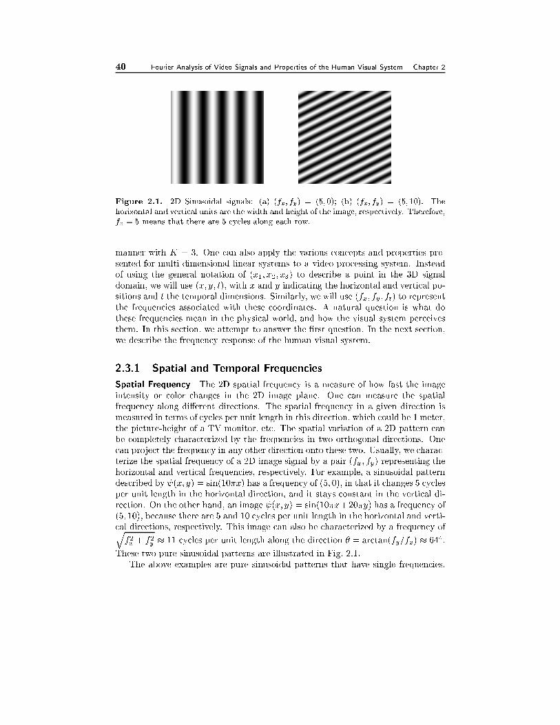
40 Fourier Analysis of Video Signals and Properties of the Human Visual System Chapter 2
Figure 2.1. 2D Sinusoidal signals: (a) (fx; fy) = (5; 0); (b) (fx; fy) = (5; 10). The
horizontal and vertical units are the width and height of the image, respectively. Therefore,
fx = 5 means that there are 5 cycles along each row.
manner with K = 3. One can also apply the various concepts and properties pre-
sented for multi-dimensional linear systems to a video processing system. Instead
of using the general notation of (x1; x2; x3) to describe a point in the 3D signal
domain, we will use (x; y; t), with x and y indicating the horizontal and vertical po-
sitions and t the temporal dimensions. Similarly, we will use (fx; fy; ft) to represent
the frequencies associated with these coordinates. A natural question is what do
these frequencies mean in the physical world, and how the visual system perceives
them. In this section, we attempt to answer the �rst question. In the next section,
we describe the frequency response of the human visual system.
2.3.1 Spatial and Temporal Frequencies
Spatial Frequency The 2D spatial frequency is a measure of how fast the image
intensity or color changes in the 2D image plane. One can measure the spatial
frequency along di�erent directions. The spatial frequency in a given direction is
measured in terms of cycles per unit length in this direction, which could be 1 meter,
the picture-height of a TV monitor, etc. The spatial variation of a 2D pattern can
be completely characterized by the frequencies in two orthogonal directions. One
can project the frequency in any other direction onto these two. Usually, we charac-
terize the spatial frequency of a 2D image signal by a pair (fx; fy) representing the
horizontal and vertical frequencies, respectively. For example, a sinusoidal pattern
described by (x; y) = sin(10�x) has a frequency of (5; 0), in that it changes 5 cycles
per unit length in the horizontal direction, and it stays constant in the vertical di-
rection. On the other hand, an image (x; y) = sin(10�x+20�y) has a frequency of
(5; 10), because there are 5 and 10 cycles per unit length in the horizontal and verti-
cal directions, respectively. This image can also be characterized by a frequency ofqf2x + f2y � 11 cycles per unit length along the direction � = arctan(fy=fx) � 64Æ:
These two pure sinusoidal patterns are illustrated in Fig. 2.1.
The above examples are pure sinusoidal patterns that have single frequencies.
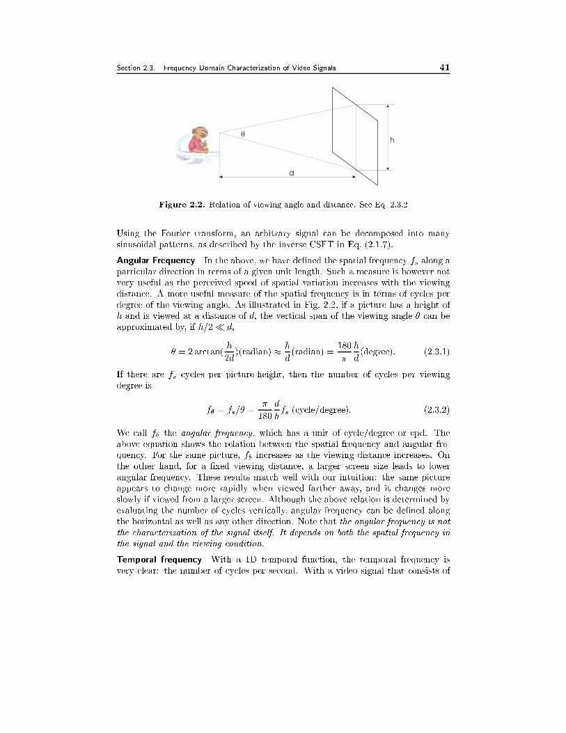
Section 2.3. Frequency Domain Characterization of Video Signals 41
d
h�
Figure 2.2. Relation of viewing angle and distance. See Eq. 2.3.2
Using the Fourier transform, an arbitrary signal can be decomposed into many
sinusoidal patterns, as described by the inverse CSFT in Eq. (2.1.7).
Angular Frequency In the above, we have de�ned the spatial frequency fs along a
particular direction in terms of a given unit length. Such a measure is however not
very useful as the perceived speed of spatial variation increases with the viewing
distance. A more useful measure of the spatial frequency is in terms of cycles per
degree of the viewing angle. As illustrated in Fig. 2.2, if a picture has a height of
h and is viewed at a distance of d, the vertical span of the viewing angle � can be
approximated by, if h=2� d;
� = 2arctan(h
2d)(radian) �
h
d(radian) =
180
�
h
d(degree): (2.3.1)
If there are fs cycles per picture-height, then the number of cycles per viewing
degree is
f� = fs=� =�
180
d
hfs (cycle=degree): (2.3.2)
We call f� the angular frequency, which has a unit of cycle/degree or cpd. The
above equation shows the relation between the spatial frequency and angular fre-
quency. For the same picture, f� increases as the viewing distance increases. On
the other hand, for a �xed viewing distance, a larger screen size leads to lower
angular frequency. These results match well with our intuition: the same picture
appears to change more rapidly when viewed farther away, and it changes more
slowly if viewed from a larger screen. Although the above relation is determined by
evaluating the number of cycles vertically, angular frequency can be de�ned along
the horizontal as well as any other direction. Note that the angular frequency is notthe characterization of the signal itself. It depends on both the spatial frequency inthe signal and the viewing condition.
Temporal frequency With a 1D temporal function, the temporal frequency is
very clear: the number of cycles per second. With a video signal that consists of
42 Fourier Analysis of Video Signals and Properties of the Human Visual System Chapter 2
varying 2D frames, the temporal frequency is 2D position dependent. For a �xed
2D position (x; y), its temporal frequency is de�ned as the number of cycles per
second, usually denoted by Hz. The maximum temporal frequency of a video refers
to the maximum of the temporal frequencies at all points in the imaged area.
2.3.2 Temporal Frequencies Caused by Linear Motion
The temporal frequency of a video signal depends on the rate at which the imaged
scene varies, which may be due to camera motion, object motion, or both. There
are usually many objects in the scene, which may be undergoing di�erent motions.
Therefore, it is not easy to relate the motion and the temporal frequency directly.
Here, we consider the temporal frequency associated with an object that is under-
going a linear motion (i.e., with a constant velocity). The analysis also applies when
the entire scene is undergoing a global linear motion, e.g., due to camera transla-
tion. As we will see, the temporal frequency depends not only on the motion, butalso the spatial frequency of the object.
Let the image pattern of the object at time 0 be described by 0(x; y) and its
velocities in horizontal and vertical directions by vx and vy : If the scene is under
homogeneous ambient illumination, so that the same object point will have the
same image intensity at di�erent times, then the image pattern at time t will be
(x; y; t) = 0(x� vxt; y � vyt); (2.3.3)
because the point (x; y) at time t correspond to the point (x�vxt; y�vyt) at time 0
(see Fig. 2.3). This is known as the constant intensity assumption. Conditions underwhich this assumption is valid will be explained further in Sec. 5.2, Eq. (5.2.11).
Performing CSFT for the above signal, we obtain
(fx; fy; ft) =
Z Z Z (x; y; t) exp (�j2�(fxx+ fyy + ftt)) dxdydt
=
Z Z 0(x � vxt; y � vyt) exp (�j2�(fx(x� vxt) + fy(y � vyt)) dxdy
�
Zexp (�j2�(ft + fxvx + fyvy)t) dt
= 0(fx; fy)
Zexp (�j2�(ft + fxvx + fyvy)t) dt
= 0(fx; fy)Æ(ft + fxvx + fyvy);
where 0(fx; fy) represents the 2D CSFT of 0(x; y):
The above result shows that (fx; fy; ft) is non-zero only on the plane de�ned
by
ft + fxvx + fyvy = 0: (2.3.4)
This means that a spatial pattern characterized by (fx; fy) in the object will lead
to a temporal frequency
ft = �fxvx � fyvy; (2.3.5)
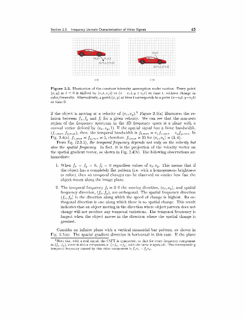
Section 2.3. Frequency Domain Characterization of Video Signals 43
(v ,v )x y
(x+v t, y+x v t)y
(x+v t, y+x v t)y
(x,y)
(x,y)
t=0 t >0
Figure 2.3. Illustration of the constant intensity assumption under motion. Every point
(x; y) at t = 0 is shifted by (vxt; vyt) to (x + vxt; y + vyt) at time t, without change in
color/intensity. Alternatively, a point (x; y) at time t corresponds to a point (x�vxt; y�vyt)
at time 0.
if the object is moving at a velocity of (vx; vy):5 Figure 2.4(a) illustrates the re-
lation between fx; fy and ft for a given velocity. We can see that the non-zero
region of the frequency spectrum in the 3D frequency space is a plane with a
normal vector de�ned by (vx; vy; 1): If the spatial signal has a �nite bandwidth,
(fx;max; fy;max), then, the temporal bandwidth is ft;max = vxfx;max + vyfy;max: In
Fig. 2.4(a), fx;max = fy;max = 5, therefore, ft;max = 35 for (vx; vy) = (3; 4):
From Eq. (2.3.5), the temporal frequency depends not only on the velocity butalso the spatial frequency. In fact, it is the projection of the velocity vector on
the spatial gradient vector, as shown in Fig. 2.4(b). The following observations are
immediate:
1. When fx = fy = 0, ft = 0 regardless values of vx; vy: This means that if
the object has a completely at pattern (i.e. with a homogeneous brightness
or color), then no temporal changes can be observed no matter how fast the
object moves along the image plane.
2. The temporal frequency ft = 0 if the moving direction, (vx; vy), and spatial
frequency direction, (fx; fy), are orthogonal. The spatial frequency direction
(fx; fy) is the direction along which the speed of change is highest. Its or-
thogonal direction is one along which there is no spatial change. This result
indicates that an object moving in the direction where object pattern does not
change will not produce any temporal variations. The temporal frequency is
largest when the object moves in the direction where the spatial change is
greatest.
Consider an in�nite plane with a vertical sinusoidal bar pattern, as shown in
Fig. 2.1(a). The spatial gradient direction is horizontal in this case. If the plane
5Note that with a real signal, the CSFT is symmetric, so that for every frequency component
at (fx; fy), there is also a component at (�fx;�fy) with the same magnitude. The corresponding
temporal frequency caused by this other component is fxvx + fyvy:
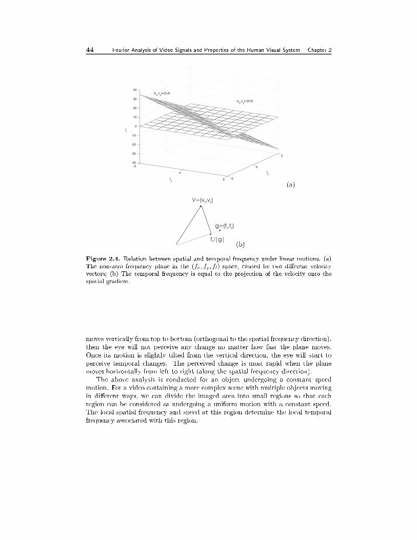
44 Fourier Analysis of Video Signals and Properties of the Human Visual System Chapter 2
-5
0
5 -5
0
5
-40
-30
-20
-10
0
10
20
30
40
fy
(vx,v
y)=(0,0)
fx
(vx,v
y)=(3,4)
ft
(a)
f /|g|t
V=(v ,v )x y
g=(f ,f )x y
(b)
Figure 2.4. Relation between spatial and temporal frequency under linear motions. (a)
The non-zero frequency plane in the (fx; fy; ft) space, caused by two di�erent velocity
vectors; (b) The temporal frequency is equal to the projection of the velocity onto the
spatial gradient.
moves vertically from top to bottom (orthogonal to the spatial frequency direction),
then the eye will not perceive any change no matter how fast the plane moves.
Once its motion is slightly tilted from the vertical direction, the eye will start to
perceive temporal changes. The perceived change is most rapid when the plane
moves horizontally from left to right (along the spatial frequency direction).
The above analysis is conducted for an object undergoing a constant speed
motion. For a video containing a more complex scene with multiple objects moving
in di�erent ways, we can divide the imaged area into small regions so that each
region can be considered as undergoing a uniform motion with a constant speed.
The local spatial frequency and speed at this region determine the local temporal
frequency associated with this region.
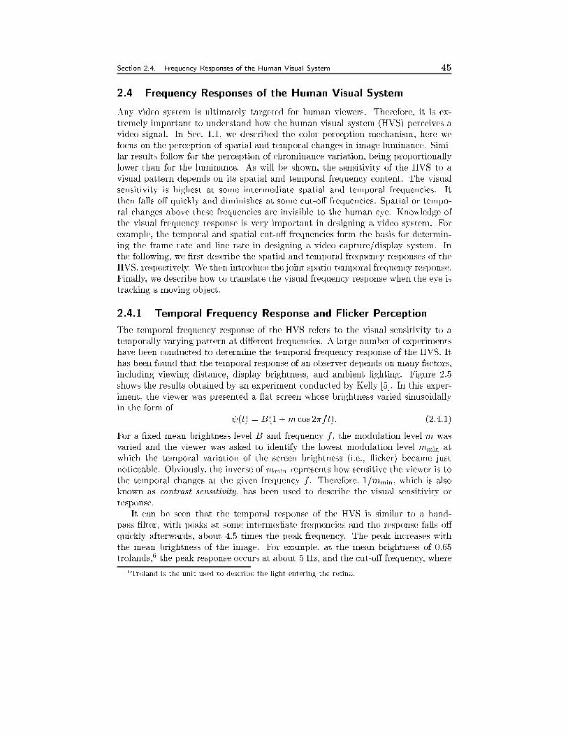
Section 2.4. Frequency Responses of the Human Visual System 45
2.4 Frequency Responses of the Human Visual System
Any video system is ultimately targeted for human viewers. Therefore, it is ex-
tremely important to understand how the human visual system (HVS) perceives a
video signal. In Sec. 1.1, we described the color perception mechanism, here we
focus on the perception of spatial and temporal changes in image luminance. Simi-
lar results follow for the perception of chrominance variation, being proportionally
lower than for the luminance. As will be shown, the sensitivity of the HVS to a
visual pattern depends on its spatial and temporal frequency content. The visual
sensitivity is highest at some intermediate spatial and temporal frequencies. It
then falls o� quickly and diminishes at some cut-o� frequencies. Spatial or tempo-
ral changes above these frequencies are invisible to the human eye. Knowledge of
the visual frequency response is very important in designing a video system. For
example, the temporal and spatial cut-o� frequencies form the basis for determin-
ing the frame rate and line rate in designing a video capture/display system. In
the following, we �rst describe the spatial and temporal frequency responses of the
HVS, respectively. We then introduce the joint spatio-temporal frequency response.
Finally, we describe how to translate the visual frequency response when the eye is
tracking a moving object.
2.4.1 Temporal Frequency Response and Flicker Perception
The temporal frequency response of the HVS refers to the visual sensitivity to a
temporally varying pattern at di�erent frequencies. A large number of experiments
have been conducted to determine the temporal frequency response of the HVS. It
has been found that the temporal response of an observer depends on many factors,
including viewing distance, display brightness, and ambient lighting. Figure 2.5
shows the results obtained by an experiment conducted by Kelly [5]. In this exper-
iment, the viewer was presented a at screen whose brightness varied sinusoidally
in the form of
(t) = B(1 +m cos 2�ft): (2.4.1)
For a �xed mean brightness level B and frequency f , the modulation level m was
varied and the viewer was asked to identify the lowest modulation level mmin at
which the temporal variation of the screen brightness (i.e., icker) became just
noticeable. Obviously, the inverse of mmin represents how sensitive the viewer is to
the temporal changes at the given frequency f . Therefore, 1=mmin, which is also
known as contrast sensitivity, has been used to describe the visual sensitivity or
response.
It can be seen that the temporal response of the HVS is similar to a band-
pass �lter, with peaks at some intermediate frequencies and the response falls o�
quickly afterwards, about 4.5 times the peak frequency. The peak increases with
the mean brightness of the image. For example, at the mean brightness of 0.65
trolands,6 the peak response occurs at about 5 Hz, and the cut-o� frequency, where
6Troland is the unit used to describe the light entering the retina.
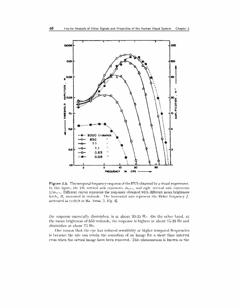
46 Fourier Analysis of Video Signals and Properties of the Human Visual System Chapter 2
Figure 2.5. The temporal frequency response of the HVS obtained by a visual experiment.
In this �gure, the left vertical axis represents mmin, and right vertical axis represents
1=mmin. Di�erent curves represent the responses obtained with di�erent mean brightness
levels, B, measured in trolands. The horizontal axis represent the icker frequency f ,
measured in cycle/s or Hz. From [5, Fig. 4].
the response essentially diminishes, is at about 20-25 Hz. On the other hand, at
the mean brightness of 850 trolands, the response is highest at about 15-20 Hz and
diminishes at about 75 Hz.
One reason that the eye has reduced sensitivity at higher temporal frequencies
is because the eye can retain the sensation of an image for a short time interval
even when the actual image have been removed. This phenomenon is known as the
Section 2.4. Frequency Responses of the Human Visual System 47
persistency of vision.7 On one hand, this causes temporal blurring of the observed
pattern, if a pattern changes at a rate faster than the refresh rate of the HVS. The
visual response falls o� very quickly beyond this frequency. On the other hand, this
vision persistency allows the display of a video signal as a consecutive set of frames.
As long as the frame interval is shorter than the vision persistency period, then the
eye perceives a continuously varying imagery. When the frame interval is longer
than this period, the eye will observe frame icker, which refers to the perception
of discontinuous frames. The lowest frame rate at which the eye does not perceive
icker is known as the critical icker frequency. By de�nition, this is equivalent
to the temporal cut-o� frequency discussed previously. The frame rate used by a
video capture/display system should exceed the critical icker frequency to avoid
the perception of icker.
From Fig. 2.5, the critical icker frequency ranges from 20 to 80 Hz, depending
on the mean brightness of the display. The brighter is the display, the higher is
the critical frequency. In a movie theater, the mean brightness is very low; on the
other hand, the CRT display is much brighter, close to 9600 trolands [8]. This is
why the movie system can use a lower frame rate than the TV system. Presently,
the movie industry uses 24 frame/second (fps), while the TV industry uses 50 (in
PAL and SECAM systems) and 60 fps (in NTSC system).8 We can see that these
frame rates are close to the cut-o� frequencies associated with the mean brightness
levels in their intended applications. Computer displays use a much higher rate,
72 fps, because a computer user sits much closer to the screen than does a TV
viewer, and at a shorter distance the visual threshold is higher. More discussion on
how to determine the spatial-temporal sampling rates of a video system is given in
Sec. 3.3.1.
2.4.2 Spatial Frequency Response
The spatial frequency response of the HVS refers to the visual sensitivity to a
stationary spatial pattern with di�erent spatial frequencies. Assuming the visual
sensitivity is isotropic with respect to the direction of spatial variation, then the
spatial frequency response can be evaluated with respect to an arbitrary spatial
direction, usually the horizontal or vertical direction is used.9 For the response to
be independent of the viewing distance, the spatial frequency response is normally
expressed as a function of the angular frequency. A large number of experiments
have been done to evaluate the spatial frequency response of the HVS. It has been
found that the spatial frequency response of the HVS is also similar to a band-pass
7This is caused by the temporal summation mechanism of the HVS, which integrates the incom-
ing light. The Bloch's law says that the integration or persistency period is inversely proportional
to the intensity of the light [10]. The brighter is the light source, the shorter is the integration
period. This makes the eye have higher temporal sensitivity when the display is brighter, which
is consistent with the results shown in Fig. 2.5.8These are actually the �eld rates, as discussed before.9Actually, visual sensitivity is higher to changes in the horizontal and vertical directions than
in the other directions.
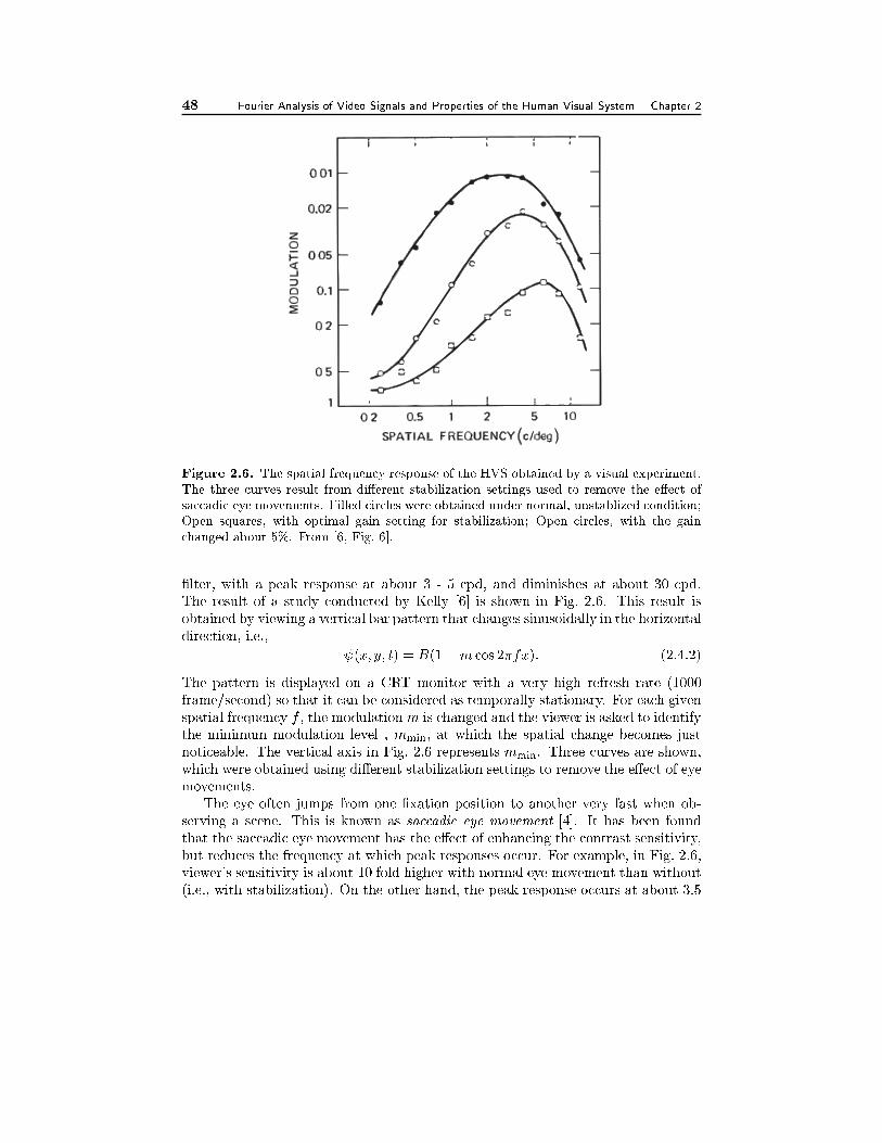
48 Fourier Analysis of Video Signals and Properties of the Human Visual System Chapter 2
Figure 2.6. The spatial frequency response of the HVS obtained by a visual experiment.
The three curves result from di�erent stabilization settings used to remove the e�ect of
saccadic eye movements. Filled circles were obtained under normal, unstablized condition;
Open squares, with optimal gain setting for stabilization; Open circles, with the gain
changed about 5%. From [6, Fig. 6].
�lter, with a peak response at about 3 - 5 cpd, and diminishes at about 30 cpd.
The result of a study conducted by Kelly [6] is shown in Fig. 2.6. This result is
obtained by viewing a vertical bar pattern that changes sinusoidally in the horizontal
direction, i.e.,
(x; y; t) = B(1 +m cos 2�fx): (2.4.2)
The pattern is displayed on a CRT monitor with a very high refresh rate (1000
frame/second) so that it can be considered as temporally stationary. For each given
spatial frequency f , the modulation m is changed and the viewer is asked to identify
the minimum modulation level , mmin; at which the spatial change becomes just
noticeable. The vertical axis in Fig. 2.6 represents mmin. Three curves are shown,
which were obtained using di�erent stabilization settings to remove the e�ect of eye
movements.
The eye often jumps from one �xation position to another very fast when ob-
serving a scene. This is known as saccadic eye movement [4]. It has been found
that the saccadic eye movement has the e�ect of enhancing the contrast sensitivity,
but reduces the frequency at which peak responses occur. For example, in Fig. 2.6,
viewer's sensitivity is about 10 fold higher with normal eye movement than without
(i.e., with stabilization). On the other hand, the peak response occurs at about 3.5
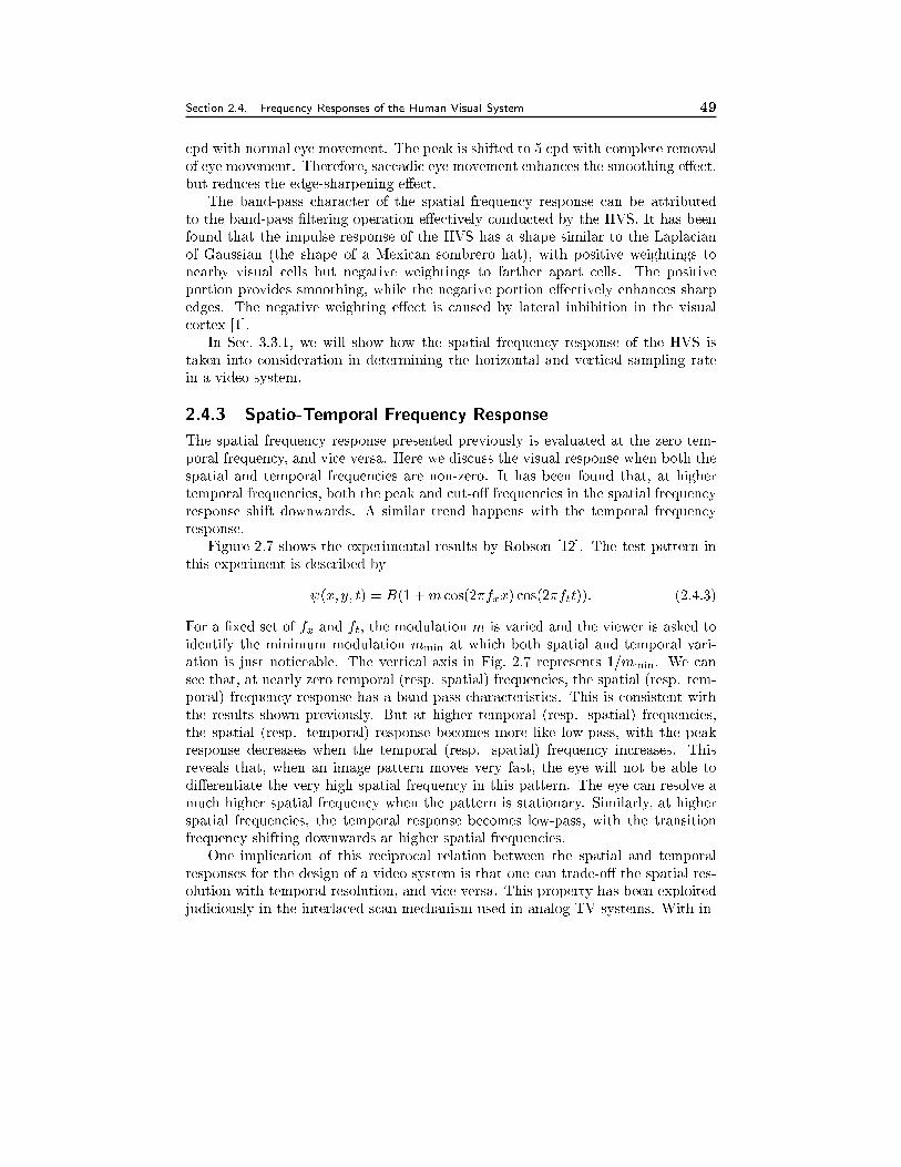
Section 2.4. Frequency Responses of the Human Visual System 49
cpd with normal eye movement. The peak is shifted to 5 cpd with complete removal
of eye movement. Therefore, saccadic eye movement enhances the smoothing e�ect,
but reduces the edge-sharpening e�ect.
The band-pass character of the spatial frequency response can be attributed
to the band-pass �ltering operation e�ectively conducted by the HVS. It has been
found that the impulse response of the HVS has a shape similar to the Laplacian
of Gaussian (the shape of a Mexican sombrero hat), with positive weightings to
nearby visual cells but negative weightings to farther apart cells. The positive
portion provides smoothing, while the negative portion e�ectively enhances sharp
edges. The negative weighting e�ect is caused by lateral inhibition in the visual
cortex [1].
In Sec. 3.3.1, we will show how the spatial frequency response of the HVS is
taken into consideration in determining the horizontal and vertical sampling rate
in a video system.
2.4.3 Spatio-Temporal Frequency Response
The spatial frequency response presented previously is evaluated at the zero tem-
poral frequency, and vice versa. Here we discuss the visual response when both the
spatial and temporal frequencies are non-zero. It has been found that, at higher
temporal frequencies, both the peak and cut-o� frequencies in the spatial frequency
response shift downwards. A similar trend happens with the temporal frequency
response.
Figure 2.7 shows the experimental results by Robson [12]. The test pattern in
this experiment is described by
(x; y; t) = B(1 +m cos(2�fxx) cos(2�ftt)): (2.4.3)
For a �xed set of fx and ft, the modulation m is varied and the viewer is asked to
identify the minimum modulation mmin at which both spatial and temporal vari-
ation is just noticeable. The vertical axis in Fig. 2.7 represents 1=mmin. We can
see that, at nearly zero temporal (resp. spatial) frequencies, the spatial (resp. tem-
poral) frequency response has a band-pass characteristics. This is consistent with
the results shown previously. But at higher temporal (resp. spatial) frequencies,
the spatial (resp. temporal) response becomes more like low-pass, with the peak
response decreases when the temporal (resp. spatial) frequency increases. This
reveals that, when an image pattern moves very fast, the eye will not be able to
di�erentiate the very high spatial frequency in this pattern. The eye can resolve a
much higher spatial frequency when the pattern is stationary. Similarly, at higher
spatial frequencies, the temporal response becomes low-pass, with the transition
frequency shifting downwards at higher spatial frequencies.
One implication of this reciprocal relation between the spatial and temporal
responses for the design of a video system is that one can trade-o� the spatial res-
olution with temporal resolution, and vice versa. This property has been exploited
judiciously in the interlaced scan mechanism used in analog TV systems. With in-
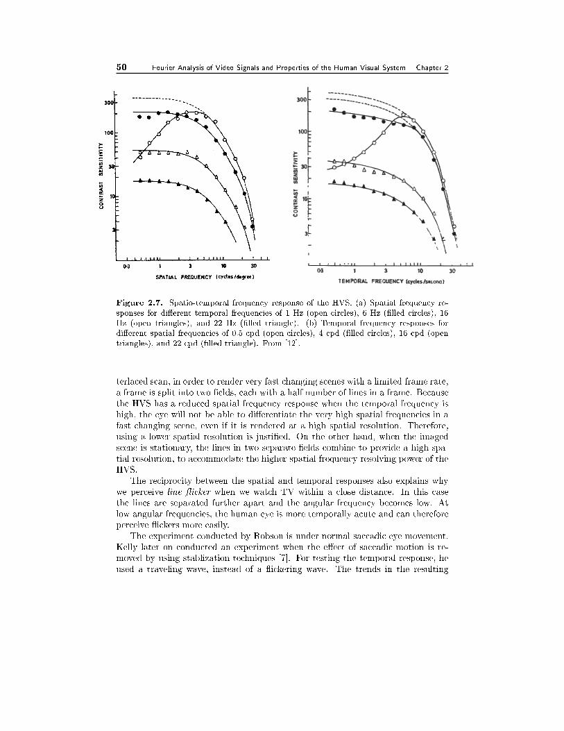
50 Fourier Analysis of Video Signals and Properties of the Human Visual System Chapter 2
Figure 2.7. Spatio-temporal frequency response of the HVS. (a) Spatial frequency re-
sponses for di�erent temporal frequencies of 1 Hz (open circles), 6 Hz (�lled circles), 16
Hz (open triangles), and 22 Hz (�lled triangle). (b) Temporal frequency responses for
di�erent spatial frequencies of 0.5 cpd (open circles), 4 cpd (�lled circles), 16 cpd (open
triangles), and 22 cpd (�lled triangle). From [12].
terlaced scan, in order to render very fast changing scenes with a limited frame rate,
a frame is split into two �elds, each with a half number of lines in a frame. Because
the HVS has a reduced spatial frequency response when the temporal frequency is
high, the eye will not be able to di�erentiate the very high spatial frequencies in a
fast changing scene, even if it is rendered at a high spatial resolution. Therefore,
using a lower spatial resolution is justi�ed. On the other hand, when the imaged
scene is stationary, the lines in two separate �elds combine to provide a high spa-
tial resolution, to accommodate the higher spatial frequency resolving power of the
HVS.
The reciprocity between the spatial and temporal responses also explains why
we perceive line icker when we watch TV within a close distance. In this case
the lines are separated further apart and the angular frequency becomes low. At
low angular frequencies, the human eye is more temporally acute and can therefore
perceive ickers more easily.
The experiment conducted by Robson is under normal saccadic eye movement.
Kelly later on conducted an experiment when the e�ect of saccadic motion is re-
moved by using stablization techniques [7]. For testing the temporal response, he
used a traveling wave, instead of a ickering wave. The trends in the resulting
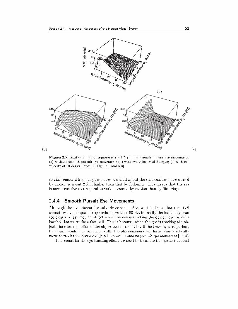
Section 2.4. Frequency Responses of the Human Visual System 51
(a)
(b) (c)
Figure 2.8. Spatio-temporal response of the HVS under smooth pursuit eye movements.
(a) without smooth pursuit eye movement; (b) with eye velocity of 2 deg/s; (c) with eye
velocity of 10 deg/s. From [3, Figs. 5.1 and 5.3]
spatial-temporal frequency responses are similar, but the temporal response caused
by motion is about 2 fold higher than that by ickering. This means that the eye
is more sensitive to temporal variations caused by motion than by ickering.
2.4.4 Smooth Pursuit Eye Movements
Although the experimental results described in Sec. 2.4.1 indicate that the HVS
cannot resolve temporal frequencies more than 80 Hz, in reality the human eye can
see clearly a fast moving object when the eye is tracking the object, e.g., when a
baseball batter tracks a fast ball. This is because, when the eye is tracking the ob-
ject, the relative motion of the object becomes smaller. If the tracking were perfect,
the object would have appeared still. The phenomenon that the eyes automatically
move to track the observed object is known as smooth pursuit eye movement [11, 4].To account for the eye tracking e�ect, we need to translate the spatio-temporal
52 Fourier Analysis of Video Signals and Properties of the Human Visual System Chapter 2
frequency at the display screen to the retina coordinate when the eye is moving [3].
Assuming the eye is moving with a speed of vx and vy, then the image observed
at the retina coordinate, ~ (x; y; t); is related to the image at the display screen,
(x; y; t), by
~ (x; y; t) = (x + vxt; y + vyt; t): (2.4.4)
Taking CSFT on both sides yield
~(fx; fy; ft) = (fx; fy; ft � vxfx � vyfy): (2.4.5)
The above relation means that the observed frequencies in the retina, ( ~fx; ~fy; ~ft),
is related to the frequencies in the display screen, (fx; fy; ft), by
~fx = fx; ~fy = fy; ~ft = ft + vxfx + vyfy: (2.4.6)
When the temporal frequency of the displayed object is zero, the perceived tem-
poral frequency increases with the eye motion speed as well as the spatial frequencies
of the observed object. When the displayed object is moving with a constant speed,
recall that the resulting temporal frequency is described by (2.3.5). Therefore, the
e�ective temporal frequency at the retina is zero, when the eye movement matches
that of the object movement. In general, by tracking the object motion, the e�ective
temporal frequency at the retina becomes smaller.
Using the coordinate transformation of Eq. (2.4.6), Girod redrew the visual
frequency response measured by Robson. Figure 2.8 shows the visual frequency
response without smooth pursuit eye movement, and that under two di�erent eye
movement speeds. Clearly, the smooth-pursuit eye movement has the e�ect of
extending the non-zero region of the visual response to a larger temporal frequency
range. In fact, temporal frequencies up to 1000 Hz can be perceived [3, 13].
Smooth pursuit eye movements have important consequences for the design of
video display and processing systems, as suggested by Girod [3]. In order to avoid
visible blur of fast moving objects, the display system needs to be able to display
temporal frequencies up to 1000 Hz. Likewise, any type of temporal �ltering has to
be carried out with motion compensation (i.e., �ltering along the motion trajectory)
to avoid visible blur of the picture content.
2.5 Summary
Fourier Analysis of Multi-dimensional Signals and Systems (Secs. 2.1,2.2)
� A K-dimensional continuous (resp. discrete) signal can be represented by
a continuous (resp. discrete) space Fourier transform (Eqs. (2.1.6,2.1.7) for
CSFT or Eqs. (2.2.3,2.2.4) for DSFT). The inverse transform means that the
signal can be decomposed into in�nitely many complex sinusoidal functions
with di�erent frequencies.
Section 2.5. Summary 53
� A LTI system can be completely characterized by its impulse response, or
equivalently, its frequency response, the Fourier transform of the impulse re-
sponse. (Theorem 2.3)
� The input and output signals of a LTI system are related by a linear con-
volution with the impulse response in the spatial domain, or a product with
the frequency response in the transform domain, as given in Eq. (2.1.13) or
(2.1.14).
Spatial and Temporal Frequencies in Video Signals (Sec. 2.3)
� The 2D spatial frequency can be speci�ed along any two orthogonal dimen-
sions, usually horizontal and vertical directions.
� Temporal frequency of a moving object depends on its velocity as well as
its spatial frequency. More speci�cally, it only depends on the projection of
the velocity vector onto the spatial gradient direction at any position on the
object, as given by Eq. (2.3.5) and Fig. 2.4.
Spatial-Temporal Frequency Responses of the HVS (Sec. 2.4)
� The human eye is most sensitive to some intermediate spatial and temporal
frequency components. At normal viewing conditions, the eye is most sensitive
to spatial frequencies between 3-5 cpd, and temporal frequencies 5-20 Hz.
� Beyond certain cut-o� frequencies, the eye cannot perceive the spatial-temporal
variations, which occur at about 30 cpd in spatial frequency, and between 20-
80 Hz in temporal frequency. These visual thresholds set the guide lines for
designing video processing/display systems. The display system only needs
to accommodate frequencies up to twice the visual thresholds.
� The eye will not perceive individual frames as long as the frame rate (�eld
rate for interlaced display) is beyond the critical icker frequency, which is
below 80 Hz for most people.
� The visual frequency responses depend on the mean brightness of the dis-
play. In general, a brighter display can make the eye more sensitive to high
frequency components.
� By tracking a moving object, the perceived temporal frequency at the retina is
reduced. If the tracking is perfect, than the temporal frequency at the retina
plane is zero.
� The cut-o� frequencies of the HVS are driving factors for determining the
spatial and temporal sampling resolutions in video capture, processing and
display. This is further discussed in Sec. 3.3.1.
54 Fourier Analysis of Video Signals and Properties of the Human Visual System Chapter 2
2.6 Problems
2.1 The impulse response of a camera can usually be modeled by
h(x; y; t) =
�1 jxj < Tx; jyj < Ty; t 2 (0; Te);
0 otherwise;(2.6.1)
where 2Tx; 2Ty are the horizontal and vertical size of the camera aperture, Te is
the exposure time. Find the CSFT of h(x; y; t). Plot the magnitude response.
Comment on the e�ect of the parameters Tx; Ty; Te on the frequency response
of the camera.
2.2 Suppose the camera described in the previous problem is looking at a scene
that consists of a cube moving in parallel with the camera imaging plane. The
projected image on the camera plane can be described by
(x; y; t) =
�1 �B + vxt < x < B + vxt;�B < y < B;
0 otherwise(2.6.2)
Derive what is the captured signal by the camera.
2.3 What are the considerations you would use to determine the frame rate and
line number when designing a video capture/display system? Are the param-
eters chosen for NTSC color TV broadcasting appropriate?
2.4 Why does a computer monitor use a higher temporal refresh rate and more
line numbers than does a typical TV monitor?
2.5 Consider a horizontal bar pattern on a TV screen that has 100 cycle/picture-
height. If the picture-height is 1 meter, and the viewer sits at 3 meters from
the screen, what is the equivalent angular frequency in cycle/degree? What if
the viewer sits at 1 meter or 5 meters away? In either case, would the viewer
be able to perceive the vertical variation properly?
2.6 Consider an object that has a at homogeneous texture surface with maximum
spatial frequency of (fx; fy) = (3; 4) cycle/meter, and is moving at a constant
speed of (vx; vy) = (1; 1) meter/second. What is the temporal frequency of
the object surface at any point? What are the results for following di�erent
speeds (in meter/second): (4,-3), (4,0), (0,1)?
2.7 Continue from the previous problem. Suppose that the eye tracks the moving
object at a speed that is equal to the object speed. What are the perceived
temporal frequencies at the retina for the di�erent values of moving speeds?
What if the eye moves at a �xed speed of (2; 2) meter/second?
2.7 Bibliography
[1] T. N. Cornsweet. Visual Perception. Academic Press, New York, 1970.
Section 2.7. Bibliography 55
[2] D. E. Dudgeon and R. M. Mersereau. Multidimensional Digital Signal Process-ing. Prentice Hall, Englewood Cli�s, NJ, 1984.
[3] B. Girod. Motion compensation: visual aspects, accuracy, and fundamental
limits. In M. I. Sezan and R. L. Lagendijk, editors, Motion analysis and imagesequence processing, pages 126{152. Kluwer Academic Publishers, 1993.
[4] P. Hallett. Eye movements. In K. Bo�, L. Kaufman, and J. P. Thomas, ed-
itors, Handbook of Perception and Human Performance: Sensory Processes andPerception. Wiley-Interscience, 1986.
[5] D. H. Kelly. Visual responses to time-dependent stimuli. I. Amplitude sensitivity
measurements. J. Opt. Soc. Am., 51:422{429, 1961.
[6] D. H. Kelly. Motion and vision. I. Stabilized images of stationary gratings. J.Opt. Soc. Am., 69:1266{1274, 1979.
[7] D. H. Kelly. Motion and vision. II. Stabilized spatio-temporal threshold surface.
J. Opt. Soc. Am., 69:1340{1349, 1979.
[8] A. N. Netravali and B. G. Haskell. Digital Pictures - Representation, Compres-sion and Standards. Plenum Press, 2nd edition, 1995.
[9] A. V. Oppenheim and R. W. Schafer. Discrete-Time Signal Processing. PrenticeHall, 1989.
[10] W. G. Owen. Spatio-temporal intergration in the human peripheral retina.
Vision Research, 12:1011{1026, 1972.
[11] D. A. Robinson. The mechanics of human smooth pursuit eye movement. J.Physiology, 180(3):569{591, Oct. 1965.
[12] J. G. Robson. Spatial and temporal contrast sensitivity functions of the visual
system. J. Opt. Soc. Am., 56:1141{1142, Aug. 1966.
[13] G. J. Tonge. Time-sampled motion portrayal. In Proc. Second InternationalConf. Image Processing and Its Applications, London, 1986.
Chapter 3
VIDEO SAMPLING
The very beginning step of any digital video processing task is the conversion of
an intrinsically continuous video signal to a digital one. The digitization process
consists of two steps: sampling and quantization. This could be implemented by a
digital camera, which directly digitizes the video of a continuous physical scene, or
by digitizing an analog signal produced by an analog camera. We also frequently
need to convert a digital video signal from one format (in terms spatial and temporal
resolution) to another, e.g., converting a video recorded in the PAL format to the
NTSC format. In this chapter we consider the sampling problem. The sampling rate
conversion problem will be discussed in the next Chapter. The quantization problem
is discussed later in Chap. 8 together with other means for signal compression.
When designing a video sampling system, three questions need to be resolved:
1) what are the necessary sampling frequencies in the spatial and temporal direc-
tions, 2) given an overall sampling rate (i.e., product of the horizontal, vertical, and
temporal sampling rates), how to sample in the 3D space to obtain the best repre-
sentation, and 3) how can we avoid the sampling artifact known as aliasing, given
that we can only use a �nite sampling rate. In this chapter, we start by describing
the general theory for sampling a multi-dimensional signal, which relates the fre-
quency spectrum of a signal and its necessary sampling pattern (Secs. 3.1 and 3.2).
We then focus on the sampling of video signals (Sec. 3.3). We will �rst describe
the factors that determine the necessary sampling rates for video and trade-o�s
that are often made in practical systems. We then discuss 2D sampling schemes
and compare the progressive and interlaced scans. We also consider how to sample
a color video, and as an example, revisit the BT.601 format. Then we introduce
several 3D sampling lattices and compare their eÆciency. Finally, we will describe
how common video cameras and displays accomplish pre-�ltering and interpolation
functions implicitly, and some practical limitations (Sec. 3.4).
3.1 Basics of the Lattice Theory
In this and next section, we extend the well-known sampling theorem for 1D and 2D
signals to a general multi-dimensional space. Recall that, for 1D signals, samples
are usually taken at a regular spacing. With 2D signals, samples are normally taken
56
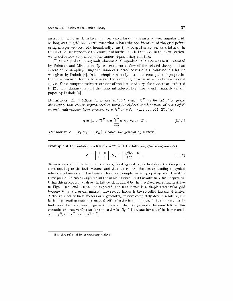
Section 3.1. Basics of the Lattice Theory 57
on a rectangular grid. In fact, one can also take samples on a non-rectangular grid,
as long as the grid has a structure that allows the speci�cation of the grid points
using integer vectors. Mathematically, this type of grid is known as a lattice. In
this section, we introduce the concept of lattice in a K-D space. In the next section,
we describe how to sample a continuous signal using a lattice.
The theory of sampling multi-dimensional signals on a lattice was �rst presented
by Petersen and Middleton [7]. An excellent review of the related theory and an
extension to sampling using the union of selected cosets of a sub-lattice in a lattice
was given by Dubois [4]. In this chapter, we only introduce concepts and properties
that are essential for us to analyze the sampling process in a multi-dimensional
space. For a comprehensive treatment of the lattice theory, the readers are referred
to [2]. The de�nitions and theorems introduced here are based primarily on the
paper by Dubois [4].
De�nition 3.1: A lattice, �, in the real K-D space, RK, is the set of all possi-
ble vectors that can be represented as integer-weighted combinations of a set of K
linearly independent basis vectors, vk 2 RK ; k 2 K = f1; 2; : : : ;Kg: That is,
� = fx 2 RK jx =
KXk=1
nkvk ;8nk 2 Zg: (3.1.1)
The matrix V = [v1;v2; � � � ;vK ] is called the generating matrix.1
Example 3.1: Consider two lattices in R2 with the following generating matrices:
V1 =
�1 0
0 1
�;V2 =
� p3=2 0
1=2 1
�: (3.1.2)
To sketch the actual lattice from a given generating matrix, we �rst draw the two points
corresponding to the basis vectors, and then determine points corresponding to typical
integer combinations of the basis vectors, for example, v1 + v2;v1 � v2; etc. Based on
these points, we can extrapolate all the other possible points usually by visual inspection.
Using this procedure, we draw the lattices determined by the two given generating matrices
in Figs. 3.1(a) and 3.1(b). As expected, the �rst lattice is a simple rectangular grid
because V1 is a diagonal matrix. The second lattice is the so-called hexagonal lattice.
Although a set of basis vectors or a generating matrix completely de�nes a lattice, the
basis or generating matrix associated with a lattice is non-unique. In fact, one can easily
�nd more than one basis or generating matrix that can generate the same lattice. For
example, one can verify that for the lattice in Fig. 3.1(b), another set of basis vectors is
v1 = [p3=2; 1=2]T ;v2 = [
p3; 0]T :
1It is also referred to as sampling matrix.
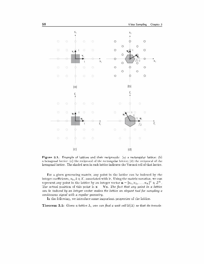
58 Video Sampling Chapter 3
(a)
(c) (d)
(b)
v2
v1
x1
x2
u1
u2
f1
f2
u1
u2
f1
f2
v2v2
v1v1
x2
x1
1
1
1
11
1
31
32
32
2/3
Figure 3.1. Example of lattices and their reciprocals: (a) a rectangular lattice; (b)
a hexagonal lattice; (c) the reciprocal of the rectangular lattice; (d) the reciprocal of the
hexagonal lattice. The shaded area in each lattice indicates the Voronoi cell of that lattice.
For a given generating matrix, any point in the lattice can be indexed by the
integer coeÆcients, nk; k 2 K; associated with it. Using the matrix notation, we canrepresent any point in the lattice by an integer vector n = [n1; n2; : : : ; nK ]
T 2 ZK :
The actual position of this point is x = Vn: The fact that any point in a lattice
can be indexed by an integer vector makes the lattice an elegant tool for sampling a
continuous signal with a regular geometry.
In the following, we introduce some important properties of the lattice.
Theorem 3.1: Given a lattice �, one can �nd a unit cell U(�) so that its transla-
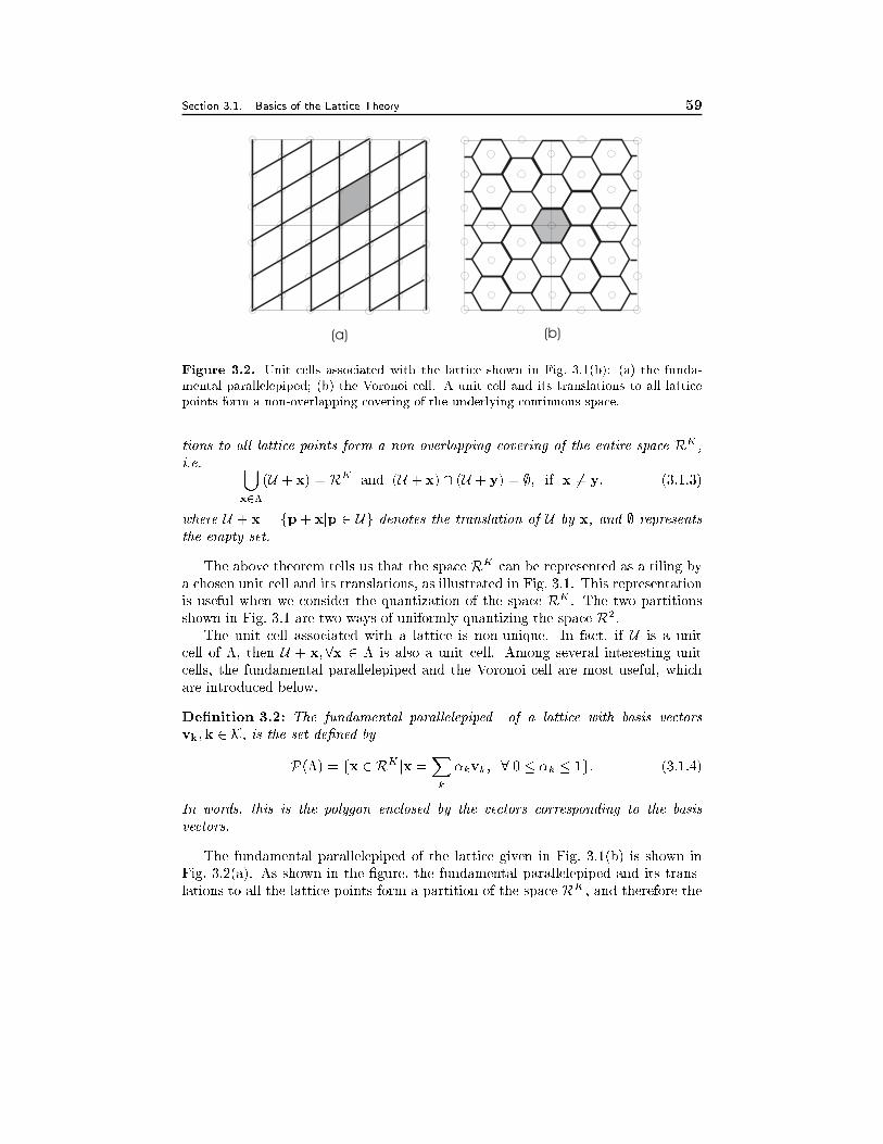
Section 3.1. Basics of the Lattice Theory 59
(a) (b)
Figure 3.2. Unit cells associated with the lattice shown in Fig. 3.1(b): (a) the funda-
mental parallelepiped; (b) the Voronoi cell. A unit cell and its translations to all lattice
points form a non-overlapping covering of the underlying continuous space.
tions to all lattice points form a non-overlapping covering of the entire space RK,
i.e. [x2�
(U + x) = RK and (U + x) \ (U + y) = ;; if x 6= y; (3.1.3)
where U + x = fp + xjp 2 Ug denotes the translation of U by x, and ; representsthe empty set.
The above theorem tells us that the space RK can be represented as a tiling by
a chosen unit cell and its translations, as illustrated in Fig. 3.1. This representation
is useful when we consider the quantization of the space RK . The two partitions
shown in Fig. 3.1 are two ways of uniformly quantizing the space R2.
The unit cell associated with a lattice is non-unique. In fact, if U is a unit
cell of �, then U + x;8x 2 � is also a unit cell. Among several interesting unit
cells, the fundamental parallelepiped and the Voronoi cell are most useful, which
are introduced below.
De�nition 3.2: The fundamental parallelepiped of a lattice with basis vectors
vk;k 2 K; is the set de�ned by
P(�) = fx 2 RK jx =Xk
�kvk ; 8 0 � �k � 1g: (3.1.4)
In words, this is the polygon enclosed by the vectors corresponding to the basis
vectors.
The fundamental parallelepiped of the lattice given in Fig. 3.1(b) is shown in
Fig. 3.2(a). As shown in the �gure, the fundamental parallelepiped and its trans-
lations to all the lattice points form a partition of the space RK ; and therefore the
60 Video Sampling Chapter 3
Lattice point
Line connecting origin to a nearest lattice point
Equidistant line
(0,0)
Figure 3.3. Determining the Voronoi cell by drawing equidistant lines.
fundamental parallelepiped is a unit cell. Obviously, there are many fundamen-
tal parallelepipeds associated with a lattice, because of the non-uniqueness of the
generating basis.
De�nition 3.3: The Voronoi cell of a lattice is the set of points which are closer
to the origin than any other points in the lattice. That is:
V(�) = fx 2 RK jd(x;0) � d(x;p);8p 2 �g: (3.1.5)
The Voronoi cell of the lattice given in Fig. 3.1(b) is shown in Fig. 3.2(b). As
with the fundamental parallelepiped, the Voronoi cell and its translations to all the
lattice points also form a partition of the space RK : Therefore, the Voronoi cell is
also a unit cell. We will see that the Voronoi cell is very useful for analyzing the
sampling process. In Fig. 3.1, the shaded region in each lattice indicates its Voronoi
cell. As expected, the Voronoi cell of a rectangular lattice is simply a rectangle.
The Voronoi cell of the second lattice is a hexagon with 6 equal length sides. This
is why the lattice is called the hexagonal lattice.
In the 2D case, the Voronoi cell of a lattice can be determined by �rst drawing a
straight line between the origin and each one of the closest non-zero lattice points,
and then drawing a perpendicular line that is half way between the two points. This
line is the equidistant line between the origin and this lattice point. The polygon
formed by all such equidistant lines surrounding the origin is then the Voronoi cell.
This is illustrated in Fig. 3.3. In the 3D case, the above procedure can be extended
by replacing the equidistant lines by equidistant planes.
Volume of the Unit Cell and Sampling Density Note that although the unit cell
associated with a lattice is not unique, the volume of the unit cell is unique. This is
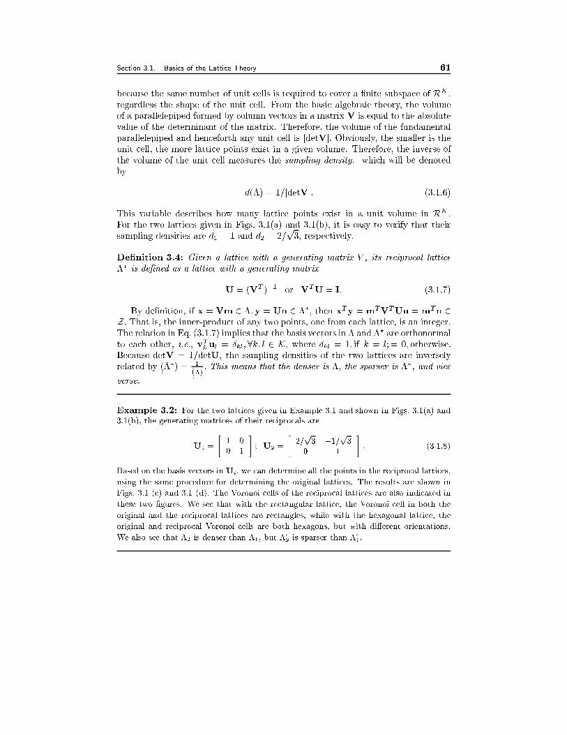
Section 3.1. Basics of the Lattice Theory 61
because the same number of unit cells is required to cover a �nite subspace of RK ,
regardless the shape of the unit cell. From the basic algebraic theory, the volume
of a parallelepiped formed by column vectors in a matrix V is equal to the absolute
value of the determinant of the matrix. Therefore, the volume of the fundamental
parallelepiped and henceforth any unit cell is jdetVj: Obviously, the smaller is theunit cell, the more lattice points exist in a given volume. Therefore, the inverse of
the volume of the unit cell measures the sampling density, which will be denoted
by
d(�) = 1=jdetVj: (3.1.6)
This variable describes how many lattice points exist in a unit volume in RK .
For the two lattices given in Figs. 3.1(a) and 3.1(b), it is easy to verify that their
sampling densities are d1 = 1 and d2 = 2=p3, respectively.
De�nition 3.4: Given a lattice with a generating matrix V , its reciprocal lattice
�� is de�ned as a lattice with a generating matrix
U = (VT )�1 or VTU = I: (3.1.7)
By de�nition, if x = Vm 2 �;y = Un 2 ��; then xTy =mTVTUn =mTn 2Z : That is, the inner-product of any two points, one from each lattice, is an integer.
The relation in Eq. (3.1.7) implies that the basis vectors in � and �� are orthonormalto each other, i.e., vTk ul = Ækl;8k; l 2 K; where Ækl = 1; if k = l; = 0; otherwise:
Because detV = 1=detU, the sampling densities of the two lattices are inversely
related by (.��) = 1
(.�): This means that the denser is �; the sparser is ��, and vice
verse.
Example 3.2: For the two lattices given in Example 3.1 and shown in Figs. 3.1(a) and
3.1(b), the generating matrices of their reciprocals are
U1 =
�1 0
0 1
�; U2 =
�2=p3 �1=
p3
0 1
�: (3.1.8)
Based on the basis vectors in Ui, we can determine all the points in the reciprocal lattices,
using the same procedure for determining the original lattices. The results are shown in
Figs. 3.1 (c) and 3.1 (d). The Voronoi cells of the reciprocal lattices are also indicated in
these two �gures. We see that with the rectangular lattice, the Voronoi cell in both the
original and the reciprocal lattices are rectangles, while with the hexagonal lattice, the
original and reciprocal Voronoi cells are both hexagons, but with di�erent orientations.
We also see that �2 is denser than �1, but ��
2 is sparser than ��
1.
62 Video Sampling Chapter 3
Theorem 3.2: Let �1 and �2 represent two lattices with generating matrices V1
and V2, respectively. If V�11V2 is a matrix of rational numbers, then the intersec-
tion
�1 \ �2 = fx 2 RK jx 2 �1 and x 2 �2gis also a lattice, and it is the largest lattice that is contained in both �1 and �2:
Under the same condition, the sum
�1 +�2 = fx+ yj8x 2 �1;8y 2 �2g
is also a lattice and it is the smallest lattice that contains both �1 and �2. Further-
more, (�1 +�2)� = ��
1\ ��
2.
Theorem 3.3: If �1 � �2, then ��1� ��
2: Also, if �1 � �2, V(�1) � V(�2):
The above results can be proven by making use of the fact that a lattice must
contain points that can be represented as Vn where n 2 ZK and V is a non-
singular matrix. The usefulness of this theorem will become clear in Sec. 4.1 when
we discussion sampling rate conversion.
Characterization of the Periodicity Using the Lattice Concept
We are all familiar with the concept of periodicity in 1D. We say a function is
periodic with a period of T if (x) = (x+nT );8n 2 Z : One important applicationof the concept of lattice is for describing the periodicity of a multi-dimensional
function, as de�ned below.
De�nition 3.5: A function is periodic with a non-singular periodicity matrix V if
(x) = (x+Vn), for any n 2 ZK.
Obviously, the set of all repetition centers, Vn;n 2 ZK ; form a lattice with
a generating matrix V. For this reason, when a lattice is used to describe the
periodicity of a function, it is also referred to as a periodicity lattice. Recall that
the entire space RK can be partitioned into in�nitely many shifted versions of a
unit cell of the lattice. Therefore, one can think of a periodic function as one that
repeats a basic pattern over a chosen unit cell at all other translated unit cells. We
call the Voronoi cell of the lattice as the fundamental period of this function. For a
1D function with a period of T; the fundamental period is the interval centered at
the origin, (�T=2; T=2): A periodic function essentially consists of its fundamental
period and the shifted versions of this period over all lattice points. Obviously, one
only needs to specify a periodic function over its fundamental period.
3.2 Sampling Over Lattices
The lattice structure provides an elegant tool for sampling a continuous signal with
a uniform but not necessarily rectangular or more generally hyper-cubic grid. It
Section 3.2. Sampling Over Lattices 63
enables one to index all samples with integer vectors, which simpli�es the description
of the resulting sampled signal. Sampling over a lattice is a generalization of uniform
sampling over a rectangular grid in 2D or a hyper-cubic grid in K-D. As shown
later, with this sampling structure, all the theorems known for 1D and 2D uniform
sampling still apply. In particular, a generalized Nyquist sampling theory exists,
which governs the necessary density and structure of the sampling lattice for a given
signal spectrum.
3.2.1 Sampling Process and Sampled Space Fourier Transform
De�nition 3.6: Given a continuous signal c(x);x 2 RK ; a sampled signal over
a lattice � with a generating matrix V is de�ned as:
s(n) = c(Vn); n 2 ZK (3.2.1)
An alternative way of de�ning the sampled signal is by considering it as a continuous-
space signal with impulses at the sampled points, i.e.,
s(x) =Xn2ZK
s(n)Æ(x�Vn);x 2 RK ; (3.2.2)
Previously in Sec.2.2, we de�ned discrete space Fourier transform (DSFT). Sim-
ilarly, we can de�ne the Fourier transform of a sampled signal over a lattice [5, 4].
Here we call it sampled space Fourier transform (SSFT). Compared to DSFT,
which is de�ned in terms of the abstract indices of sampled points, the de�nition
of SSFT keeps the underlying sampling structure of a discrete signal in the picture,
and enables one to make connections with actual physical dimensions.
De�nition 3.7: The sampled space Fourier transform (SSFT) of a signal sampled
over a lattice � with a generating matrix V is de�ned as:
s(f) =Xn2ZK
s(n) exp(�j2�fTVn) (3.2.3)
Using the de�nition in Eq. (3.2.2), it can be shown that the CSFT of the sampled
signal is equal to the above de�ned SSFT. Thus the de�nition of the SSFT is
consistent with the CSFT. Also, the SSFT reduces to the previously de�ned DSFT
when the lattice is a hypercube, i.e., V is a K-D identity matrix.
Notice that because exp(j2�fTx) = 1; if fTx = n 2 Z , we haves(f +Um) = s(f); with U = (VT )�1:
This means that the SSFT is periodic with a periodicity matrix U; and that the
spectral repetition centers fall on the reciprocal of the sampling lattice, ��: Thefundamental period is the Voronoi cell of the reciprocal lattice, V(��). For this
reason, one only needs to specify the SSFT of a sampled signal over V(��). This
basic pattern repeats at all points in the reciprocal lattice. This is illustrated in
Fig. 3.4. We will come back to this �gure later.
64 Video Sampling Chapter 3
Theorem 3.4 (The Inverse Sampled Space Fourier Transform) A sampled
signal over a lattice � with generating matrix V can be obtained from its SSFT by
s(n) =1
d(�)
ZV(��)
s(f) exp(j2�fTVn)df ; for n 2 ZK (3.2.4)
The validity of the above inverse relation can be proven by substituting s(f)
in Eq. (3.2.4) with the forward transform in Eq. (3.2.3), and making use of the
equality:
ZV(��)
exp(j2�xT f)df =
�volumefV(��)g = d(�); for x = 0;
0; otherwise:(3.2.5)
The inverse relation in Eq. (3.2.4) reveals that one can represent a sampled
signal as an in�nite sum of complex exponential functions with frequencies de�ned
in the Voronoi cell of the reciprocal lattice.
All the properties of the CSFT can be carried over to the SSFT. Here we only
state the convolution theorem. The proof is straight forward and is left as an
exercise (Prob. 3.4).
De�nition 3.8: The linear convolution of two sampled signals over the same lattice
� is de�ned as:
s(n) � hs(n) =X
m2ZK s(n�m)hs(m) =
Xxm2�
c(xn � xm)hc(xm); (3.2.6)
where c(x) and hc(x) are the continuous versions of s(n) and hs(n), respectively,
and xn; n 2 ZK denote the sample positions.
Theorem 3.5 (Convolution Theorem over the Sampled Space) As with CSFT
and DSFT, the convolution of two signals in a sampled space is equivalent to the
product of their SSFT's, i.e.,
s(n) � hs(n) ! s(f)Hs(f): (3.2.7)
Characterization of Sampled Linear Shift-Invariant Systems Given a linear shift-
invariant system over the continuous space RK with an impulse response hc(x), if
one samples the input and output signals over a lattice �, it can be shown (Prob. 3.5)
that the sampled input signal s(n) = c(Vn) and output signal �s(n) = �c(Vn)
are related by the above de�ned linear convolution in �, and the �lter will be exactly
the sampled impulse response hs(n) = hc(Vn): Therefore, the sampled system is
completely characterized by the sampled impulse response hs(n).
3.2.2 The Generalized Nyquist Sampling Theorem
Theorem 3.6 (The Generalized Nyquist Sampling Theorem) If a continu-
ous signal c(x);x 2 RKis sampled over a lattice � with a generating matrix V,
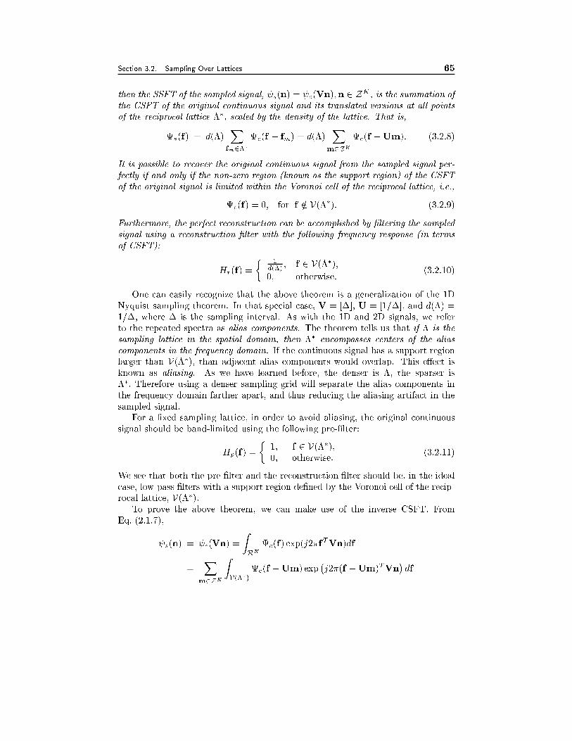
Section 3.2. Sampling Over Lattices 65
then the SSFT of the sampled signal, s(n) = c(Vn);n 2 ZK, is the summation of
the CSFT of the original continuous signal and its translated versions at all points
of the reciprocal lattice ��, scaled by the density of the lattice. That is,
s(f) = d(�)X
fm2��c(f � fm) = d(�)
Xm2ZK
c(f �Um): (3.2.8)
It is possible to recover the original continuous signal from the sampled signal per-
fectly if and only if the non-zero region (known as the support region) of the CSFT
of the original signal is limited within the Voronoi cell of the reciprocal lattice, i.e.,
c(f) = 0; for f =2 V(��): (3.2.9)
Furthermore, the perfect reconstruction can be accomplished by �ltering the sampled
signal using a reconstruction �lter with the following frequency response (in terms
of CSFT):
Hr(f) =
�1
d(�); f 2 V(��);
0; otherwise:(3.2.10)
One can easily recognize that the above theorem is a generalization of the 1D
Nyquist sampling theorem. In that special case, V = [�], U = [1=�], and d(�) =
1=�; where � is the sampling interval. As with the 1D and 2D signals, we refer
to the repeated spectra as alias components. The theorem tells us that if � is the
sampling lattice in the spatial domain, then �� encompasses centers of the alias
components in the frequency domain. If the continuous signal has a support region
larger than V(��), than adjacent alias components would overlap. This e�ect is
known as aliasing. As we have learned before, the denser is �, the sparser is
��: Therefore using a denser sampling grid will separate the alias components in
the frequency domain farther apart, and thus reducing the aliasing artifact in the
sampled signal.
For a �xed sampling lattice, in order to avoid aliasing, the original continuous
signal should be band-limited using the following pre-�lter:
Hp(f) =
�1; f 2 V(��);0; otherwise:
(3.2.11)
We see that both the pre-�lter and the reconstruction �lter should be, in the ideal
case, low-pass �lters with a support region de�ned by the Voronoi cell of the recip-
rocal lattice, V(��):To prove the above theorem, we can make use of the inverse CSFT. From
Eq. (2.1.7),
s(n) = c(Vn) =
ZRK
c(f) exp(j2�fTVn)df
=X
m2ZK
ZV(��)
c(f �Um) exp�j2�(f �Um)TVn
�df

66 Video Sampling Chapter 3
=X
m2ZK
ZV(��)
c(f �Um) exp(j2�fTVn)df
=
ZV(��)
Xm2ZK
c(f �Um) exp(j2�fTVn)df
Comparing the last equality with (3.2.4), the result in (3.2.8) follows.
Example 3.3: Consider a 2D signal with a spectrum shown in Fig. 3.4 (a), which has a
circular support region with radius r = 1=p3. If we use the lattice presented in Fig. 3.1(a)
to sample this signal, which is equivalent to using non-interlaced sampling with sampling
intervals �x = �y = 1, the spectrum of the sampled signals will be as shown in Figs. 3.4(b),
which is obtained by repeating the original spectra over points in the reciprocal lattice,
shown previously in Fig. 3.1(c). Obviously, because the signal support region is larger than
the Voronoi cell of the reciprocal lattice, there is overlap between the alias components
in the sampled spectrum. To avoid the overlap, we can pre-�lter the continuous signal so
that its spectrum is non-zero only in the Voronoi cell of the reciprocal lattice, as illustrated
in Fig. 3.4(c). If we now sample this signal with the same lattice, all the alias components
will cover the entire spectrum exactly, without overlapping, as shown in Fig. 3.4(d). The
reconstructed signal using the ideal reconstruction �lter will be exactly the same as the
pre-�ltered signal, given in Fig. 3.4(c). Obviously, this signal has lost some frequency
components compared to the original signal. If the application demands retention of the
full bandwidth of the original signal, then a sampling lattice with a reciprocal Voronoi cell
equal to or larger than the support region of the signal is needed. For example, if we use the
hexagonal lattice in Fig. 3.1(b), then the signal spectrum �ts entirely within the Voronoi
cell of its reciprocal lattice, as illustrated in Fig. 3.4(e), and the spectrum of the sampled
signal will be as shown in Fig. 3.4(f), with no aliasing. In this case, the reconstructed
signal will be perfect. Rather than using the hexagonal lattice given in Fig. 3.1(b), one
can still use a rectangular lattice, with a smaller sampling interval �x = �y =p3=2 < 1.
This will lead to a higher sampling density. Recall that the sampling densities of the �rst
and second lattices are 1 and 2=p3, respectively, as derived previously, while the above
scaled rectangular lattice has a sampling density of 4=3, higher than that of the hexagonal
lattice. From this example, we can see that the hexagonal lattice is more eÆcient than a
rectangular one, because it requires a lower sampling density to obtain alias-free sampling.
3.2.3 Sampling EÆciency
As already illustrated by Example 3.3, to avoid aliasing, the sampling lattice must
be designed so that the Voronoi cell of its reciprocal lattice completely covers the
signal spectrum. Obviously, one can always design a very dense lattice to satisfy this
requirement. This however will require a very high sampling density. To minimize
the sampling density, one should design the lattice so that its reciprocal Voronoi cell
covers the signal spectrum as tightly as possible. The solution will depend on the
signal spectrum, which in general could have an arbitrarily shaped support region.
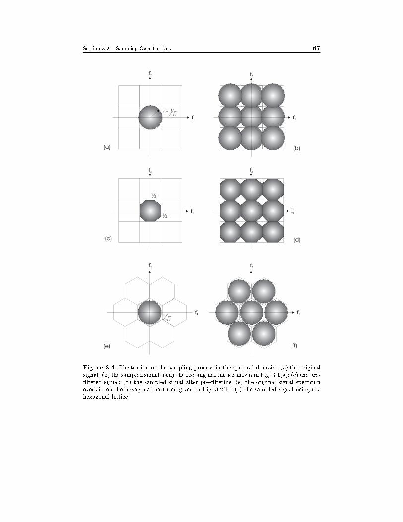
Section 3.2. Sampling Over Lattices 67
(a)
(c)
(e)
(d)
(f)
(b)
½
½
f1
f2f2
f2
f2 f2
f2
f1
f1 f1
f1f1 f1
31�r
31
Figure 3.4. Illustration of the sampling process in the spectral domain. (a) the original
signal; (b) the sampled signal using the rectangular lattice shown in Fig. 3.1(a); (c) the pre-
�ltered signal; (d) the sampled signal after pre-�ltering; (e) the original signal spectrum
overlaid on the hexagonal partition given in Fig. 3.2(b); (f) the sampled signal using the
hexagonal lattice.
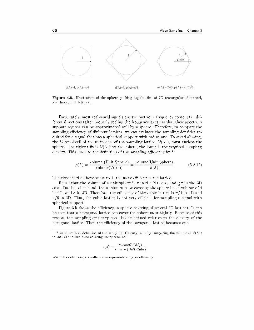
68 Video Sampling Chapter 3
�/611 1
d(������������ d( ������ ����� � 32/)(,32)( �� ����d
Figure 3.5. Illustration of the sphere packing capabilities of 2D rectangular, diamond,
and hexagonal lattices.
Fortunately, most real-world signals are symmetric in frequency contents in dif-
ferent directions (after properly scaling the frequency axes) so that their spectrum
support regions can be approximated well by a sphere. Therefore, to compare the
sampling eÆciency of di�erent lattices, we can evaluate the sampling densities re-
quired for a signal that has a spherical support with radius one. To avoid aliasing,
the Voronoi cell of the reciprocal of the sampling lattice, V(��), must enclose thesphere. The tighter �t is V(��) to the sphere, the lower is the required sampling
density. This leads to the de�nition of the sampling eÆciency by 2
�(�) =volume (Unit Sphere)
volume(V(��)) =volume(Unit Sphere)
d(�): (3.2.12)
The closer is the above value to 1, the more eÆcient is the lattice.
Recall that the volume of a unit sphere is � in the 2D case, and 4
3� in the 3D
case. On the other hand, the minimum cube covering the sphere has a volume of 4
in 2D, and 8 in 3D. Therefore, the eÆciency of the cubic lattice is �=4 in 2D and
�=6 in 3D. Thus, the cubic lattice is not very eÆcient for sampling a signal with
spherical support.
Figure 3.5 shows the eÆciency in sphere covering of several 2D lattices. It can
be seen that a hexagonal lattice can cover the sphere most tightly. Because of this
reason, the sampling eÆciency can also be de�ned relative to the density of the
hexagonal lattice. Then the eÆciency of the hexagonal lattice becomes one.
2An alternative de�nition of the sampling eÆciency [4] is by comparing the volume of V(��)
to that of the unit cube covering the sphere, i.e.,
�(�) =volume(V(��))
volume (Unit Cube):
With this de�nition, a smaller value represents a higher eÆciency.
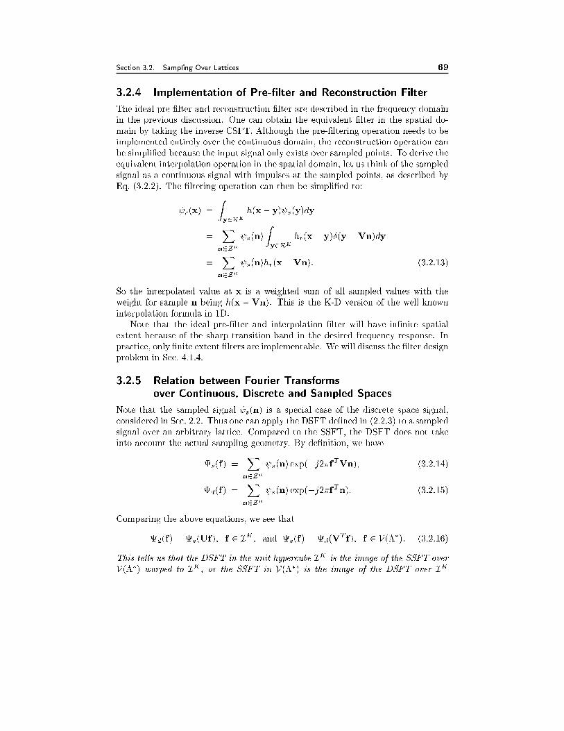
Section 3.2. Sampling Over Lattices 69
3.2.4 Implementation of Pre-�lter and Reconstruction Filter
The ideal pre-�lter and reconstruction �lter are described in the frequency domain
in the previous discussion. One can obtain the equivalent �lter in the spatial do-
main by taking the inverse CSFT. Although the pre-�ltering operation needs to be
implemented entirely over the continuous domain, the reconstruction operation can
be simpli�ed because the input signal only exists over sampled points. To derive the
equivalent interpolation operation in the spatial domain, let us think of the sampled
signal as a continuous signal with impulses at the sampled points, as described by
Eq. (3.2.2). The �ltering operation can then be simpli�ed to:
r(x) =
Zy2RK
h(x� y) s(y)dy
=Xn2ZK
s(n)
Zy2RK
hr(x � y)Æ(y �Vn)dy
=Xn2ZK
s(n)hr(x�Vn): (3.2.13)
So the interpolated value at x is a weighted sum of all sampled values with the
weight for sample n being h(x �Vn). This is the K-D version of the well known
interpolation formula in 1D.
Note that the ideal pre-�lter and interpolation �lter will have in�nite spatial
extent because of the sharp transition band in the desired frequency response. In
practice, only �nite extent �lters are implementable. We will discuss the �lter design
problem in Sec. 4.1.4.
3.2.5 Relation between Fourier Transforms
over Continuous, Discrete and Sampled Spaces
Note that the sampled signal s(n) is a special case of the discrete space signal,
considered in Sec. 2.2. Thus one can apply the DSFT de�ned in (2.2.3) to a sampled
signal over an arbitrary lattice. Compared to the SSFT, the DSFT does not take
into account the actual sampling geometry. By de�nition, we have
s(f) =Xn2ZK
s(n) exp(�j2�fTVn); (3.2.14)
d(f) =Xn2ZK
s(n) exp(�j2�fTn): (3.2.15)
Comparing the above equations, we see that
d(f) = s(Uf); f 2 IK ; and s(f) = d(VT f); f 2 V(��): (3.2.16)
This tells us that the DSFT in the unit hypercube IK is the image of the SSFT over
V(��) warped to IK , or the SSFT in V(��) is the image of the DSFT over IK
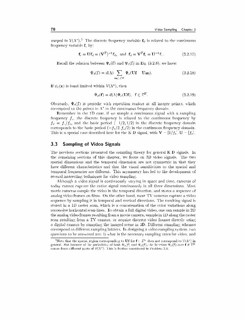
70 Video Sampling Chapter 3
warped to V(��).3 The discrete frequency variable fd is related to the continuous
frequency variable fc by:
fc = Ufd = (VT )�1fd; and fd = VT fc = U�1fc: (3.2.17)
Recall the relation between s(f) and c(f) in Eq. (3.2.8), we have:
d(f) = d(�)X
m2ZKc(Uf �Um): (3.2.18)
If c(x) is band-limited within V(��); then
d(f) = d(�)c(Uf); f 2 IK : (3.2.19)
Obviously, d(f) is periodic with repetition centers at all integer points, which
correspond to the points in �� in the continuous frequency domain.
Remember in the 1D case, if we sample a continuous signal with a sampling
frequency fs, the discrete frequency is related to the continuous frequency by
fd = fc=fs, and the basic period (�1=2; 1=2) in the discrete frequency domain
corresponds to the basic period (�fs=2; fs=2) in the continuous frequency domain.
This is a special case described here for the K-D signal, with V = [1=fs];U = [fs]:
3.3 Sampling of Video Signals
The previous sections presented the sampling theory for general K-D signals. In
the remaining sections of this chapter, we focus on 3D video signals. The two
spatial dimensions and the temporal dimension are not symmetric in that they
have di�erent characteristics and that the visual sensitivities to the spatial and
temporal frequencies are di�erent. This asymmetry has led to the development of
several interesting techniques for video sampling.
Although a video signal is continuously varying in space and time, cameras of
today cannot capture the entire signal continuously in all three dimensions. Most
movie cameras sample the video in the temporal direction, and stores a sequence of
analog video frames on �lms. On the other hand, most TV cameras capture a video
sequence by sampling it in temporal and vertical directions. The resulting signal is
stored in a 1D raster scan, which is a concatenation of the color variations along
successive horizontal scan-lines. To obtain a full digital video, one can sample in 2D
the analog video frames resulting from a movie camera, sample in 1D along the raster
scan resulting from a TV camera, or acquire discrete video frames directly using
a digital camera by sampling the imaged scene in 3D. Di�erent sampling schemes
correspond to di�erent sampling lattices. In designing a video sampling system, two
questions to be answered are: i) what is the necessary sampling rates for video, and
3Note that the spatial region corresponding to Uf for f 2 IK does not correspond to V(��) in
general. But because of the periodicity of both s(f) and d(f), the function d(f) over f 2 IK
comes from di�erent parts of V(��). This is further considered in Problem 3.6.
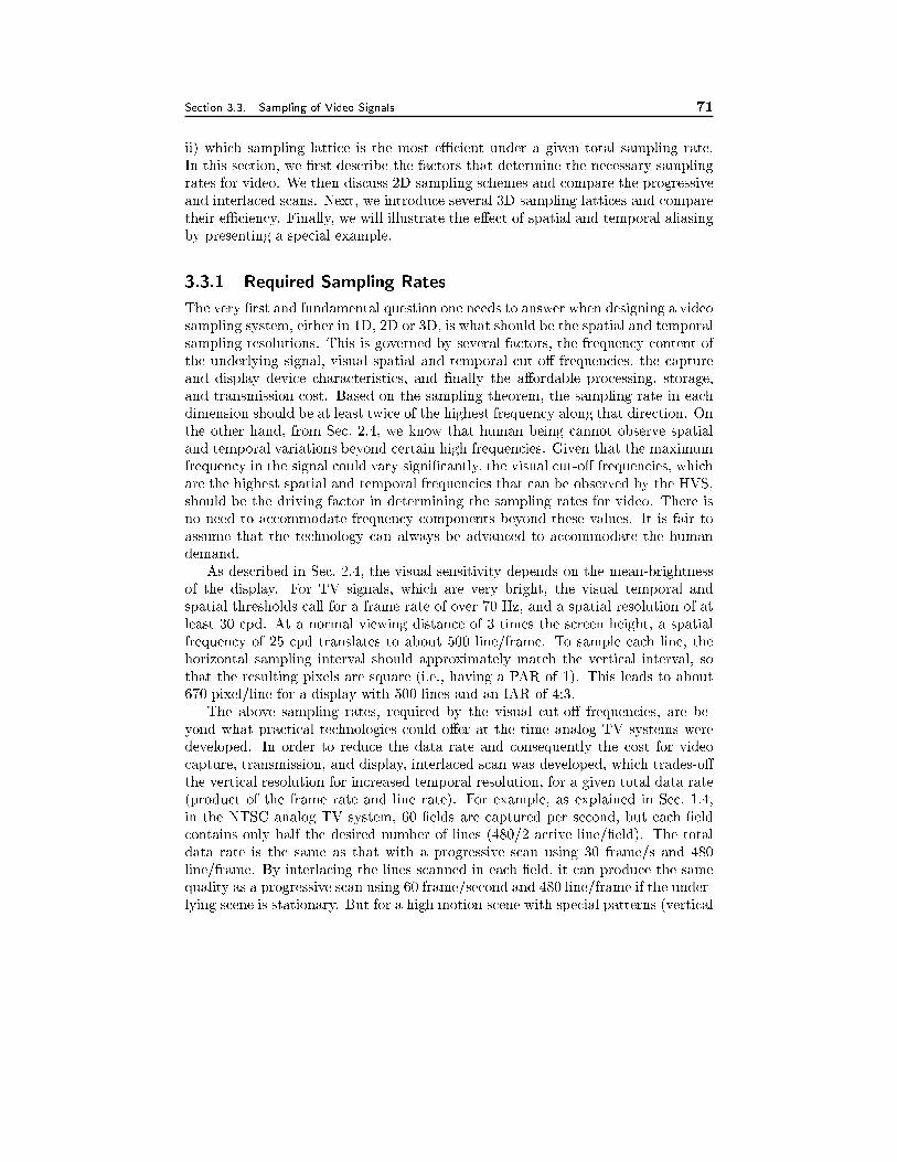
Section 3.3. Sampling of Video Signals 71
ii) which sampling lattice is the most eÆcient under a given total sampling rate.
In this section, we �rst describe the factors that determine the necessary sampling
rates for video. We then discuss 2D sampling schemes and compare the progressive
and interlaced scans. Next, we introduce several 3D sampling lattices and compare
their eÆciency. Finally, we will illustrate the e�ect of spatial and temporal aliasing
by presenting a special example.
3.3.1 Required Sampling Rates
The very �rst and fundamental question one needs to answer when designing a video
sampling system, either in 1D, 2D or 3D, is what should be the spatial and temporal
sampling resolutions. This is governed by several factors, the frequency content of
the underlying signal, visual spatial and temporal cut-o� frequencies, the capture
and display device characteristics, and �nally the a�ordable processing, storage,
and transmission cost. Based on the sampling theorem, the sampling rate in each
dimension should be at least twice of the highest frequency along that direction. On
the other hand, from Sec. 2.4, we know that human being cannot observe spatial
and temporal variations beyond certain high frequencies. Given that the maximum
frequency in the signal could vary signi�cantly, the visual cut-o� frequencies, which
are the highest spatial and temporal frequencies that can be observed by the HVS,
should be the driving factor in determining the sampling rates for video. There is
no need to accommodate frequency components beyond these values. It is fair to
assume that the technology can always be advanced to accommodate the human
demand.
As described in Sec. 2.4, the visual sensitivity depends on the mean-brightness
of the display. For TV signals, which are very bright, the visual temporal and
spatial thresholds call for a frame rate of over 70 Hz, and a spatial resolution of at
least 30 cpd. At a normal viewing distance of 3 times the screen height, a spatial
frequency of 25 cpd translates to about 500 line/frame. To sample each line, the
horizontal sampling interval should approximately match the vertical interval, so
that the resulting pixels are square (i.e., having a PAR of 1). This leads to about
670 pixel/line for a display with 500 lines and an IAR of 4:3.
The above sampling rates, required by the visual cut-o� frequencies, are be-
yond what practical technologies could o�er at the time analog TV systems were
developed. In order to reduce the data rate and consequently the cost for video
capture, transmission, and display, interlaced scan was developed, which trades-o�
the vertical resolution for increased temporal resolution, for a given total data rate
(product of the frame rate and line rate). For example, as explained in Sec. 1.4,
in the NTSC analog TV system, 60 �elds are captured per second, but each �eld
contains only half the desired number of lines (480/2 active line/�eld). The total
data rate is the same as that with a progressive scan using 30 frame/s and 480
line/frame. By interlacing the lines scanned in each �eld, it can produce the same
quality as a progressive scan using 60 frame/second and 480 line/frame if the under-
lying scene is stationary. But for a high motion scene with special patterns (vertical
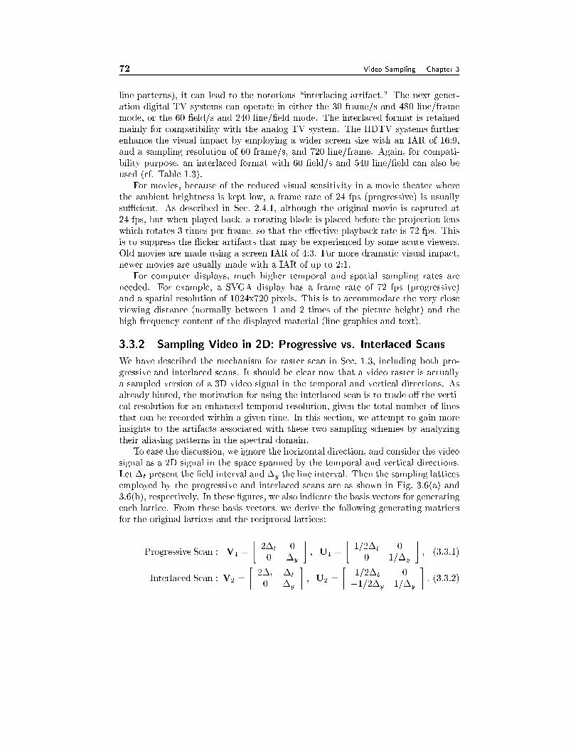
72 Video Sampling Chapter 3
line patterns), it can lead to the notorious \interlacing artifact." The next gener-
ation digital TV systems can operate in either the 30 frame/s and 480 line/frame
mode, or the 60 �eld/s and 240 line/�eld mode. The interlaced format is retained
mainly for compatibility with the analog TV system. The HDTV systems further
enhance the visual impact by employing a wider screen size with an IAR of 16:9,
and a sampling resolution of 60 frame/s, and 720 line/frame. Again, for compati-
bility purpose, an interlaced format with 60 �eld/s and 540 line/�eld can also be
used (cf. Table 1.3).
For movies, because of the reduced visual sensitivity in a movie theater where
the ambient brightness is kept low, a frame rate of 24 fps (progressive) is usually
suÆcient. As described in Sec. 2.4.1, although the original movie is captured at
24 fps, but when played back, a rotating blade is placed before the projection lens
which rotates 3 times per frame, so that the e�ective playback rate is 72 fps. This
is to suppress the icker artifacts that may be experienced by some acute viewers.
Old movies are made using a screen IAR of 4:3. For more dramatic visual impact,
newer movies are usually made with a IAR of up to 2:1.
For computer displays, much higher temporal and spatial sampling rates are
needed. For example, a SVGA display has a frame rate of 72 fps (progressive)
and a spatial resolution of 1024x720 pixels. This is to accommodate the very close
viewing distance (normally between 1 and 2 times of the picture height) and the
high frequency content of the displayed material (line graphics and text).
3.3.2 Sampling Video in 2D: Progressive vs. Interlaced Scans
We have described the mechanism for raster scan in Sec. 1.3, including both pro-
gressive and interlaced scans. It should be clear now that a video raster is actually
a sampled version of a 3D video signal in the temporal and vertical directions. As
already hinted, the motivation for using the interlaced scan is to trade o� the verti-
cal resolution for an enhanced temporal resolution, given the total number of lines
that can be recorded within a given time. In this section, we attempt to gain more
insights to the artifacts associated with these two sampling schemes by analyzing
their aliasing patterns in the spectral domain.
To ease the discussion, we ignore the horizontal direction, and consider the video
signal as a 2D signal in the space spanned by the temporal and vertical directions.
Let �t present the �eld interval and �y the line interval. Then the sampling lattices
employed by the progressive and interlaced scans are as shown in Fig. 3.6(a) and
3.6(b), respectively. In these �gures, we also indicate the basis vectors for generating
each lattice. From these basis vectors, we derive the following generating matrices
for the original lattices and the reciprocal lattices:
Progressive Scan : V1 =
�2�t 0
0 �y
�; U1 =
�1=2�t 0
0 1=�y
�; (3.3.1)
Interlaced Scan : V2 =
�2�t �t
0 �y
�; U2 =
�1=2�t 0
�1=2�y 1=�y
�: (3.3.2)
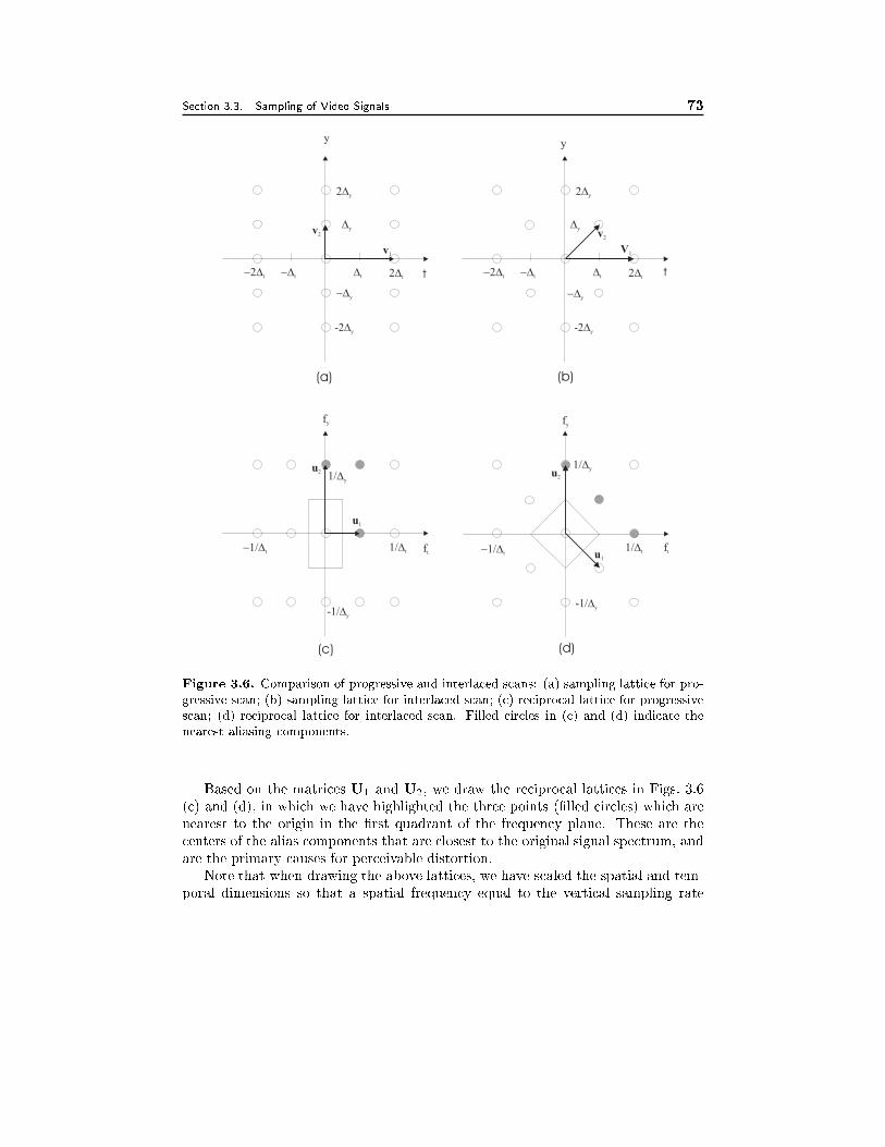
Section 3.3. Sampling of Video Signals 73
y
v1
u1
u2 u2
u1
v2 v2
V1
2�y
-2�y
�y
�t��t �t� �t
��y
t
y
2�y
-2�y
�y
�t��t �t� �t
��y
t
��y
-1/�y
��t���t ft
fy
��y
-1/�y
��t���tft
fy
(a)
(c) (d)
(b)
Figure 3.6. Comparison of progressive and interlaced scans: (a) sampling lattice for pro-
gressive scan; (b) sampling lattice for interlaced scan; (c) reciprocal lattice for progressive
scan; (d) reciprocal lattice for interlaced scan. Filled circles in (c) and (d) indicate the
nearest aliasing components.
Based on the matrices U1 and U2; we draw the reciprocal lattices in Figs. 3.6
(c) and (d), in which we have highlighted the three points (�lled circles) which are
nearest to the origin in the �rst quadrant of the frequency plane. These are the
centers of the alias components that are closest to the original signal spectrum, and
are the primary causes for perceivable distortion.
Note that when drawing the above lattices, we have scaled the spatial and tem-
poral dimensions so that a spatial frequency equal to the vertical sampling rate
74 Video Sampling Chapter 3
fs;y = 1=�y is assigned the same length as a temporal frequency equal to the �eld
rate fs;t = 1=�t. Similarly, the spatial interval �y and the temporal interval �t
are given the same length. Ideally, we would like to equate the temporal and spatial
frequencies based on the visual sensitivity, by assigning the same length to the spa-
tial and temporal cut-o� frequencies. Because the spatial and temporal sampling
rates are usually chosen based on the respective cut-o� frequencies, equating the
sampling frequencies in di�erent directions is in general appropriate.
Comparing the original and reciprocal lattices of these two scans, we arrive at
the following observations:
1. They have the same sampling density, i.e., d1(�) = d2(�) = 1=2�t�y:
2. They have the same nearest aliases, at 1=�y; along the vertical frequency axis.
This means that in the absence of motion, the two sampling lattices have the
same vertical resolving power. This is because although there are only half
the number of lines in each �eld, when the imaged scene is stationary, the lines
sampled in two separate �eld times appear as if they were sampled at the same
time. When there is motion in the scene, however, the vertical resolution of
the interlaced scan is lower than that of the progressive scan.
3. They have di�erent nearest aliases along the temporal frequency axis. For
the progressive scan, the �rst alias occurs at 1=2�t, while for the interlaced
scan, this occurs at 1=�t: Recall that a temporal frequency component that
is larger than half of the nearest temporal alias will cause a icker artifact.
We can see that with the interlaced scan, ickering is less likely to happen,
when the object has a at or slowly varying vertical pattern.
4. They have di�erent mixed aliases. The mixed alias is de�ned as the nearest
o�-axis alias component. A frequency component that is close to the mixed
alias causes inter-line icker and line crawl. For the progressive scan, the
mixed alias occurs at (1=2�t; 1=�y), while for the interlaced scan, this occurs
at (1=2�t; 1=2�y). Because the interlaced scan has a mixed alias that is closer
to the origin, the inter-line icker and line crawl artifacts are more visible in
interlaced scans. These are the notorious interlacing artifacts.
5. For a signal with isotropic spectral support, the interlaced scan is more eÆ-
cient. Speci�cally, the maximum radius of the signal spectrum that can be
represented without aliasing is equal to 1=4�t with the progressive scan; while
this is increased to 1=2p2�t with the interlaced scan. In interpreting this re-
sult, it is important to remember that this is based on our way of equating
the spatial and temporal frequencies.
Note that the above comparison is between an interlaced scan and a progressive
scan that have the same total sampling rate. In this case, the interlaced scan has
some advantages over progressive scans, as shown above. To improve the quality
further, the interlaced scan can be deinterlaced, to yield a progressive scan that
Section 3.3. Sampling of Video Signals 75
has twice the total sampling rate. We will consider the deinterlacing problem in
Sec. 4.2.1.
An interesting analysis of the spectrum of an interlaced frame under constant
linear motion is given by Beuker and Shah [1]. Based on this analysis, techniques
for deinterlacing and other rate conversion problems are considered.
3.3.3 Sampling a Raster Scan: BT.601 Format Revisited
As described in the beginning of this chapter, one way to obtain a full digital video
is to sample a raster scan. Recall that a raster is a 1D signal consisting of successive
horizontal scan-lines in successive frames (�elds for an interlaced raster). Therefore,
the sampling interval along the scan line directly determines the horizontal sam-
pling interval. To determine the sampling interval, several factors need to be taken
into account. First, the resulting horizontal sampling spacing should match with
the vertical spacing between scan lines so that the sampling frequencies in the hor-
izontal and vertical directions are similar. Second, the resulting samples in the 3D
space should follow a desired sampling lattice. For example, if the samples on each
frame/�eld are to form a rectangular grid, the sampling interval should be a integer
divisor of the line interval. These criteria were used in designing the BT.601 digital
video format described in Sec. 1.5.2. By selecting the sampling interval according
to Eq. (1.5.2), the samples on successive horizontal scan-lines are vertically aligned,
with the horizontal and vertical sampling spacings being approximately equal.
The above discussions assume that the underlying video raster has a single
luminance component. For a color video raster, including one luminance and two
chrominance components, a straight forward approach is to use the same sampling
frequency for all components. This will lead to the BT.601 4:4:4 format, previously
shown in Fig. 1.8(a). However, it is well known that the HVS is more sensitive to the
luminance information than to the chrominance. Therefore it is wise to sample the
chrominance components at resolutions lower than that for the luminance. Ideally,
sampling frequencies in all three dimensions should be reduced equally. However,
because a raster is a stack of horizontal scan-lines, reducing the sampling frequency
for the raster only lowers the horizontal sampling rate. The vertical and temporal
sampling rates are una�ected. For example, if the sampling rate for the chrominance
components, fs;c, is half of that for the luminance component, fs, the temporal and
vertical sampling intervals are the same for the chrominance component and the
luminance component, but the horizontal sampling interval for the chrominance is
twice of that for the luminance. This in fact is the color sub-sampling format used
in the BT.601 4:2:2 format shown previously in Fig. 1.8(b). If we down-sample the
chrominance component by a factor of 4 along the raster scan, we will arrive at
the BT.601 4:1:1 format of Fig. 1.8(c). Given a 4:2:2 signal, we can further down-
sample the vertical dimension by a factor of two, which will lead to the BT.601 4:2:0
format, given in Fig. 1.8(d). Note that the 4:2:0 format cannot be obtained directly
from the raster signal by using uniform sampling. Conversion between BT.601 4:2:2
signals to 4:2:0 signals is considered in Chapter 4, Problems 4.6 and 4.7.
76 Video Sampling Chapter 3
The 4:1:1 and the 4:2:0 formats have the same overall sample rates (samples/s),
but the 4:2:0 format can represent a video more accurately because it captures
horizontal and vertical details in the chrominance components with the same res-
olution, half of that for the luminance component. On the other hand, with the
4:1:1 format, the vertical detail is represented with the same resolution as the lu-
minance component, whereas the horizontal is represented with only a quarter of
that resolution.
The above discussion assumes that the three color components in the raster
signal are separated. To sample a composite color video, one needs to �rst separate
the individual color components and then perform sampling as discussed before.
3.3.4 Sampling Video in 3D
In the sampling schemes described in the previous section, the horizontal samples
are aligned vertically in all �elds. Such a sampling scheme is by no means optimal.
One can also take samples in an interlaced or more complicated pattern over the
x-y plane. More generally, one can directly sample the 3D space using a desired
lattice. It is diÆcult to make a camera that can implement a complicated 3D sam-
pling structure. However, one can �rst acquire samples using a dense but simply
structured lattice and then down-convert it to the desired lattice. In this section,
we compare the eÆciency of several lattices that have been used for video sampling.
The materials presented here are from [4]. To ease the presentation, we will assume
that the frequency axes, fx; fy; ft, are scaled by the maximum frequencies of the
signal, 1=fx;max; 1=fy;max; 1=ft;max, respectively. The horizontal, vertical, and tem-
poral axes, x; y; t, are correspondingly scaled by fx;max; fy;max; ft;max. The following
discussion is in terms of the scaled unit-less variables. To evaluate the sampling eÆ-
ciency of each lattice, we further assume the support region of the signal is a sphere
with radius one, in the scaled frequency space.
First, let us consider the sampling of a progressively scanned raster with frame
interval �t and line interval �y . If the samples are aligned vertically with a hor-
izontal interval of �x, then the equivalent 3D sampling lattice is simply cubic or
orthorhombic (denoted by ORT), as given in Fig. 3.7(a). Obviously, to avoid alias-
ing, we need to have �x = �y = �t =1
2, with a sampling density d(ORT) = 8:
Next, let us consider the sampling of an interlaced raster with a �eld interval of
�t=2, and line interval within each �eld 2�y. If the samples in di�erent �elds are
aligned, with horizontal interval �x, the equivalent 3D sampling lattice is illustrated
in Fig. 3.7(b), and is denoted by ALI. It can be shown that to avoid aliasing, we must
have �x = �y =1
2;�t =
1p3; which leads to a sampling density of d(ALI) = 4
p3:
This is more eÆcient that the ORT lattice.
To improve the sampling eÆciency, we can shift the samples in the even and
odd lines by half, as shown in Fig. 3.7(c). This lattice is called body-centered
orthorhombic lattice or BCO. It can be shown that the required sampling intervals
for avoiding aliasing are �x = �t =1p2;�y =
1
2
p2; with a sampling density of 4
p2:
Therefore, this lattice is more eÆcient than the ALI.
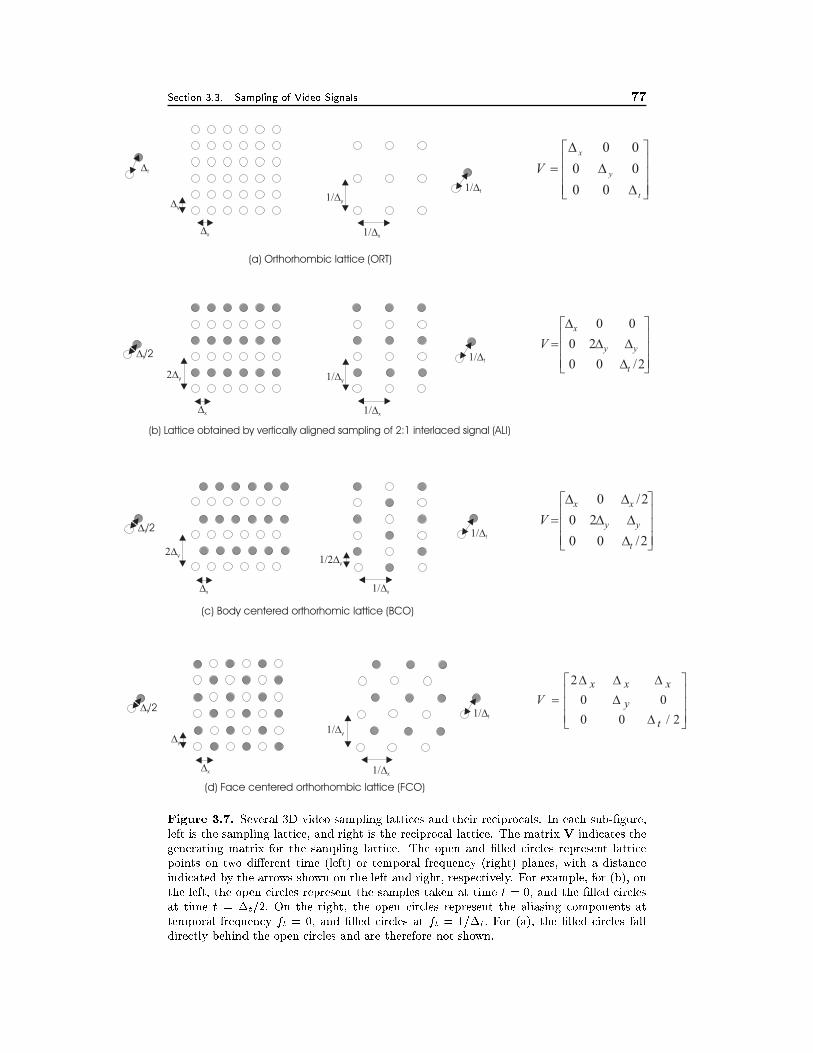
Section 3.3. Sampling of Video Signals 77
�x
�x
�x
�x
��x
��x
��x
��x
�y
�y
�y
�y
��y
��y
��y
� �y
�t
�t/2
�t/2
�t/2
��t
��t
��t
��t
(a) Orthorhombic lattice (ORT)
(b) Lattice obtained by vertically aligned sampling of 2:1 interlaced signal (ALI)
(c) Body centered orthorhomic lattice (BCO)
(d) Face centered orthorhombic lattice (FCO)
���
�
�
���
�
�
�
�
�
�
t
y
x
V
00
00
00
���
�
�
���
�
�
�
�
���
�
2/00
00
2
t
y
xxx
V
���
�
�
���
�
�
�
��
��
�
2/00
20
2/0
t
yy
xx
V
���
�
�
���
�
�
�
��
�
�
2/00
20
00
t
yy
x
V
Figure 3.7. Several 3D video sampling lattices and their reciprocals. In each sub-�gure,
left is the sampling lattice, and right is the reciprocal lattice. The matrix V indicates the
generating matrix for the sampling lattice. The open and �lled circles represent lattice
points on two di�erent time (left) or temporal frequency (right) planes, with a distance
indicated by the arrows shown on the left and right, respectively. For example, for (b), on
the left, the open circles represent the samples taken at time t = 0, and the �lled circles
at time t = �t=2: On the right, the open circles represent the aliasing components at
temporal frequency ft = 0, and �lled circles at ft = 1=�t: For (a), the �lled circles fall
directly behind the open circles and are therefore not shown.
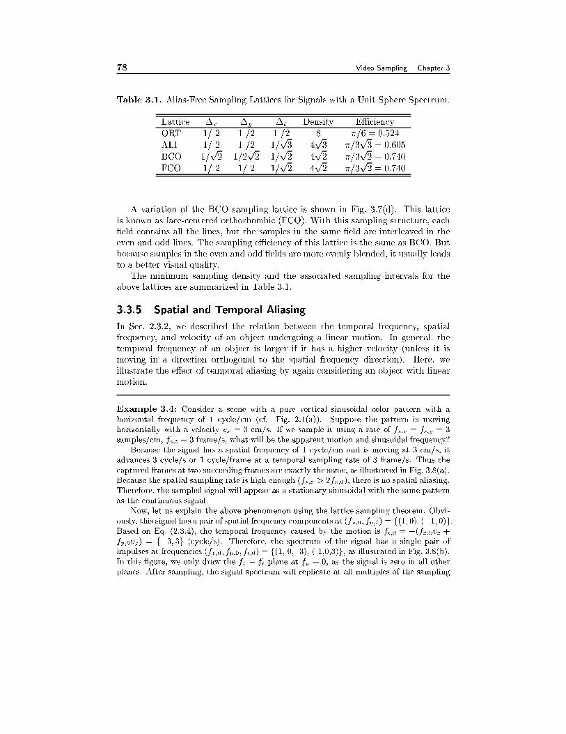
78 Video Sampling Chapter 3
Table 3.1. Alias-Free Sampling Lattices for Signals with a Unit Sphere Spectrum.
Lattice �x �y �t Density EÆciency
ORT 1/ 2 1 /2 1 /2 8 �=6 = 0:524
ALI 1/ 2 1 /2 1=p3 4
p3 �=3
p3 = 0:605
BCO 1=p2 1=2
p2 1=
p2 4
p2 �=3
p2 = 0:740
FCO 1/ 2 1/ 2 1=p2 4
p2 �=3
p2 = 0:740
A variation of the BCO sampling lattice is shown in Fig. 3.7(d). This lattice
is known as face-centered orthorhombic (FCO). With this sampling structure, each
�eld contains all the lines, but the samples in the same �eld are interleaved in the
even and odd lines. The sampling eÆciency of this lattice is the same as BCO. But
because samples in the even and odd �elds are more evenly blended, it usually leads
to a better visual quality.
The minimum sampling density and the associated sampling intervals for the
above lattices are summarized in Table 3.1.
3.3.5 Spatial and Temporal Aliasing
In Sec. 2.3.2, we described the relation between the temporal frequency, spatial
frequency, and velocity of an object undergoing a linear motion. In general, the
temporal frequency of an object is larger if it has a higher velocity (unless it is
moving in a direction orthogonal to the spatial frequency direction). Here, we
illustrate the e�ect of temporal aliasing by again considering an object with linear
motion.
Example 3.4: Consider a scene with a pure vertical sinusoidal color pattern with a
horizontal frequency of 1 cycle/cm (cf. Fig. 2.1(a)). Suppose the pattern is moving
horizontally with a velocity vx = 3 cm/s. If we sample it using a rate of fs;x = fs;y = 3
samples/cm, fs;t = 3 frame/s, what will be the apparent motion and sinusoidal frequency?
Because the signal has a spatial frequency of 1 cycle/cm and is moving at 3 cm/s, it
advances 3 cycle/s or 1 cycle/frame at a temporal sampling rate of 3 frame/s. Thus the
captured frames at two succeeding frames are exactly the same, as illustrated in Fig. 3.8(a).
Because the spatial sampling rate is high enough (fs;x > 2fx;0); there is no spatial aliasing.Therefore, the sampled signal will appear as a stationary sinusoidal with the same pattern
as the continuous signal.
Now, let us explain the above phenomenon using the lattice sampling theorem. Obvi-
ously, this signal has a pair of spatial frequency components at (fx;0; fy;0) = f(1; 0); (�1; 0)g:Based on Eq. (2.3.4), the temporal frequency caused by the motion is ft;0 = �(fx;0vx +fy;0vy) = f�3; 3g (cycle/s). Therefore, the spectrum of the signal has a single pair of
impulses at frequencies (fx;0; fy;0; ft;0) = f(1, 0, -3), (-1,0,3)g, as illustrated in Fig. 3.8(b).
In this �gure, we only draw the fx � ft plane at fy = 0, as the signal is zero in all other
planes. After sampling, the signal spectrum will replicate at all multiples of the sampling
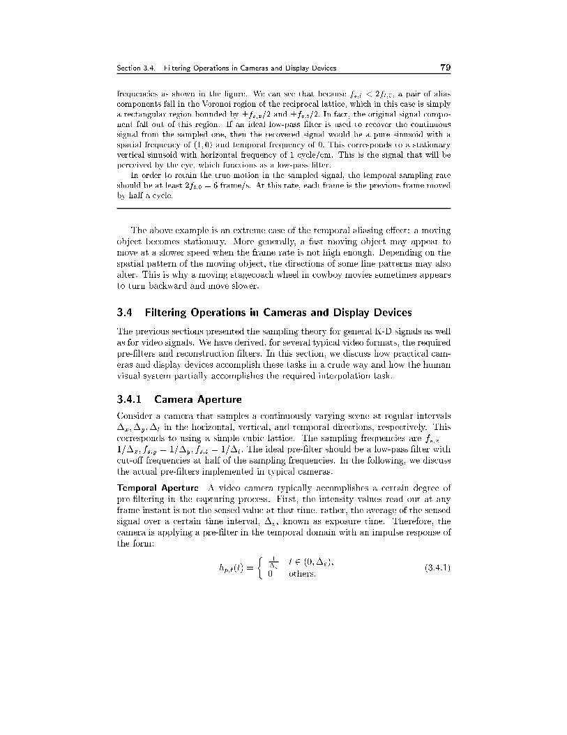
Section 3.4. Filtering Operations in Cameras and Display Devices 79
frequencies as shown in the �gure. We can see that because fs;t < 2ft;0; a pair of alias
components fall in the Voronoi region of the reciprocal lattice, which in this case is simply
a rectangular region bounded by �fs;x=2 and �fs;t=2: In fact, the original signal compo-
nent fall out of this region. If an ideal low-pass �lter is used to recover the continuous
signal from the sampled one, then the recovered signal would be a pure sinusoid with a
spatial frequency of (1; 0) and temporal frequency of 0: This corresponds to a stationary
vertical sinusoid with horizontal frequency of 1 cycle/cm. This is the signal that will be
perceived by the eye, which functions as a low-pass �lter.
In order to retain the true motion in the sampled signal, the temporal sampling rate
should be at least 2ft;0 = 6 frame/s. At this rate, each frame is the previous frame moved
by half a cycle.
The above example is an extreme case of the temporal aliasing e�ect: a moving
object becomes stationary. More generally, a fast moving object may appear to
move at a slower speed when the frame rate is not high enough. Depending on the
spatial pattern of the moving object, the directions of some line patterns may also
alter. This is why a moving stagecoach wheel in cowboy movies sometimes appears
to turn backward and move slower.
3.4 Filtering Operations in Cameras and Display Devices
The previous sections presented the sampling theory for general K-D signals as well
as for video signals. We have derived, for several typical video formats, the required
pre-�lters and reconstruction �lters. In this section, we discuss how practical cam-
eras and display devices accomplish these tasks in a crude way and how the human
visual system partially accomplishes the required interpolation task.
3.4.1 Camera Aperture
Consider a camera that samples a continuously varying scene at regular intervals
�x;�y;�t in the horizontal, vertical, and temporal directions, respectively. This
corresponds to using a simple cubic lattice. The sampling frequencies are fs;x =
1=�x; fs;y = 1=�y; fs;t = 1=�t: The ideal pre-�lter should be a low-pass �lter with
cut-o� frequencies at half of the sampling frequencies. In the following, we discuss
the actual pre-�lters implemented in typical cameras.
Temporal Aperture A video camera typically accomplishes a certain degree of
pre-�ltering in the capturing process. First, the intensity values read out at any
frame instant is not the sensed value at that time, rather, the average of the sensed
signal over a certain time interval, �e, known as exposure time. Therefore, the
camera is applying a pre-�lter in the temporal domain with an impulse response of
the form:
hp;t(t) =
�1
�et 2 (0;�e);
0 others:(3.4.1)
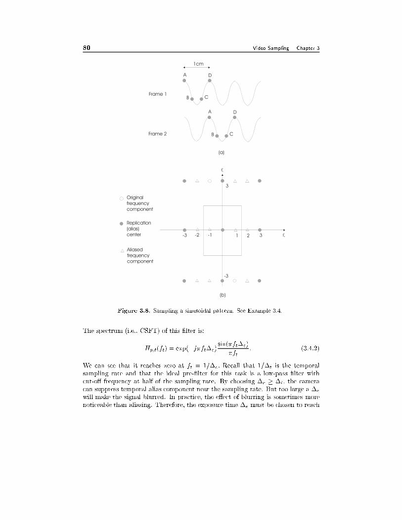
80 Video Sampling Chapter 3
ft
fx
(a)
(b)
A
B C
D
A
B C
D
Frame 1
Frame 2
Original
frequency
component
Replication
(alias)
center
Aliased
frequency
component
1cm
1 2 3-1-2-3
3
-3
Figure 3.8. Sampling a sinusoidal pattern. See Example 3.4.
The spectrum (i.e., CSFT) of this �lter is:
Hp;t(ft) = exp(�j�ft�e)sin(�ft�e)
�ft: (3.4.2)
We can see that it reaches zero at ft = 1=�e: Recall that 1=�t is the temporal
sampling rate and that the ideal pre-�lter for this task is a low-pass �lter with
cut-o� frequency at half of the sampling rate. By choosing �e � �t, the camera
can suppress temporal alias component near the sampling rate. But too large a �e
will make the signal blurred. In practice, the e�ect of blurring is sometimes more
noticeable than aliasing. Therefore, the exposure time �e must be chosen to reach

Section 3.4. Filtering Operations in Cameras and Display Devices 81
a proper trade-o� between aliasing and blurring e�ects.
Spatial Aperture In addition to temporal integration, the camera also performs
spatial integration. The value read-out at any pixel (a position on a scan line with
a tube-based camera or a sensor in a CCD camera) is not the optical signal at
that point alone, rather a weighted integration of the signals in a small window
surrounding it, called aperture. The shape of the aperture and the weighting values
constitute the camera spatial aperture function. This aperture function serves as
the spatial pre-�lter, and its Fourier transform is known as the modulation transfer
function (MTF) of the camera. With most cameras, the spatial aperture function
can be approximated by a circularly symmetric Gaussian function,
hp;x;y(x; y) =1p2��
exp��(x2 + y2)=2�2
�: (3.4.3)
The spectrum of this function is also a Gaussian:
Hp;x;y(fx; fy) = exp��(f2x + f2y )=2�
2�; with � =
1
2��: (3.4.4)
The value of � or � depends on the aperture size and shape, which are usually
designed so that the frequency response is 0:5 at half of the vertical and horizontal
sampling rates. Assuming fs;x = fs;y = fs;x;y, we see that this requires � =
fs;x;y=2pln 2: For the MTF of several camera tubes, please see [6].
Combined Aperture The overall camera aperture function or pre-�lter is
hp(x; y; t) = hp;t(t)hp;x;y(x; y); (3.4.5)
with a frequency response
Hp(fx; fy; ft) = Hp;t(ft)Hp;x;y(fx; fy): (3.4.6)
The impulse response of a camera with �e = �t = 1=60 second and fs;y = 480
(line/picture-height) is shown in Fig. 3.9(a). Its frequency response is given in
Fig. 3.9(b). Only the fy�ft plane at fx = 0 is shown. Obviously, it is far from
the ideal half-band low-pass �lter, which should have a square pass-band de�ned by
jfyj � fs;y=2; jftj � fs;t=2: On one hand, it attenuates the frequency components
inside the desired pass-band (the Voronoi cell), thereby reducing the signal resolu-
tion unnecessarily; on the other hand, it does not remove completely the frequency
components in the desired stop-band, which will cause aliasing in the sampled sig-
nal. It has been found that the human eye is more annoyed by the loss of resolution
than the aliasing artifact. This is partly because the aliasing artifact (fold-over of
an alias component) only cause noticeable visual artifacts when the image contains
high frequency periodic patterns that are close to the lowest aliasing frequency,
which are rare in natural scene imagery. For this reason, preservation of the sig-
nal in the pass-band is more important than suppression of the signal outside the
pass-band.
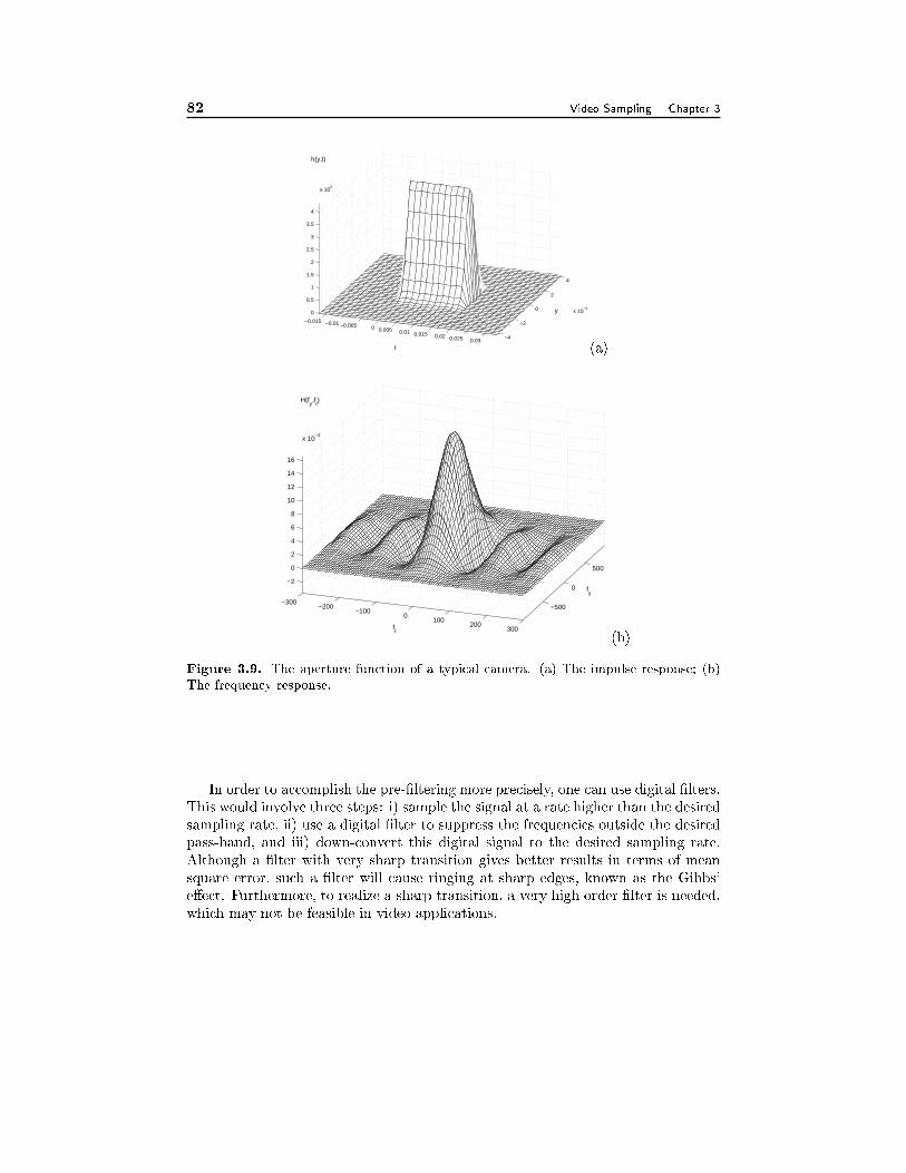
82 Video Sampling Chapter 3
−0.015 −0.01 −0.005 0 0.005 0.01 0.015 0.02 0.025 0.03 −4
−2
0
2
4
x 10−3
0
0.5
1
1.5
2
2.5
3
3.5
4
x 104
y
t
h(y,t)
(a)
−300−200
−1000
100200
300
−500
0
500
−2
0
2
4
6
8
10
12
14
16
x 10−3
fy
ft
H(fy,f
t)
(b)
Figure 3.9. The aperture function of a typical camera. (a) The impulse response; (b)
The frequency response.
In order to accomplish the pre-�ltering more precisely, one can use digital �lters.
This would involve three steps: i) sample the signal at a rate higher than the desired
sampling rate, ii) use a digital �lter to suppress the frequencies outside the desired
pass-band, and iii) down-convert this digital signal to the desired sampling rate.
Although a �lter with very sharp transition gives better results in terms of mean
square error, such a �lter will cause ringing at sharp edges, known as the Gibbs'
e�ect. Furthermore, to realize a sharp transition, a very high order �lter is needed,
which may not be feasible in video applications.
Section 3.5. Summary 83
3.4.2 Display Aperture
As described in Sec. 1.2, with a CRT monitor, an electronic gun emits an electronic
beam across the screen line by line, striking phosphors with intensities proportional
to the intensity of the video signal at corresponding locations. To display a color
image, three beams are emitted by three separate guns, striking red, green, and
blue phosphors with the desired intensity combination at each location. The beam
thickness essentially determines the vertical �ltering: a very thin beam will make
the image looks sharper but will also cause the perception of the scan lines if the
viewer sits too close to the screen; on the other hand, a thicker beam will blur the
image. Normally to minimize the loss of spatial resolution, thin beams are used
so that very little vertical �ltering is exercised by the display device. Temporal
�ltering is determined by the phosphors used. The P22 phosphors used in color
television decay to less than 10 percent of peak responses in 10 �s to 1 ms [3, 4],
much shorter than a �eld time (16.7 ms). Thus virtually no temporal �ltering is
performed.
Fortunately, the human visual system (HVS) has a low-pass or band-pass char-
acteristic, depending on the regime of the temporal and spatial frequencies in the
imagery. This has been described in Sec. 2.4. Therefore, the eye performs to some
degree the required interpolation task. For improved performance, one can use a
digital �lter to �rst up-convert the sampled signal to a higher resolution, which is
then fed to a high resolution display system.
It has been found that the combination of the camera and display apertures in
most of current television systems results in a maximum vertical resolution of only
about 0.7 of the theoretical limit (i.e. half of the line rate). In other words, the
maximum vertical frequency that can be rendered properly by a TV system with
a line number of Ny is about 0:7Ny=2. This factor is referred to as the Kell factor
[4], denoted by K. For a discussion of how the parameters of an imaging system
can in uence the Kell factor, the reader is referred to [8]. By using digital �lters
for pre-�ltering and interpolation, as described before, Kell factors much closer to
unity may be possible. Previously, in Sec. 1.4.3, we have seen how does the Kell
factor a�ect the bandwidth of the TV signal.
3.5 Summary
Sampling of K-D Signals over Arbitrary Lattices (Sec. 3.2)
� A K-D continuous space signal can be sampled over a lattice. One can de�ne
a sampled space Fourier transform (SSFT), which satis�es similar properties
as DSFT.
� A SSFT is periodic with alias centers located at points of the reciprocal of the
sampling lattice.
� The original signal can be reconstructed perfectly from the sampled signal if
the spectrum (i.e., CSFT) of the original signal is non-zero only within the
84 Video Sampling Chapter 3
Voronoi cell of the reciprocal lattice.
� A sampling lattice is more eÆcient if the Voronoi cell of its reciprocal lattice
covers the support region of the signal more tightly. For example, for a sig-
nal with circular spectrum support, the rectangular sampling lattice is less
eÆcient than a hexagonal or diamond lattice.
Sampling of Video Signals (Sec. 3.3)
� The spatial and temporal sampling frequencies required for a video signal
depend on the cut-o� frequencies of the spatio-temporal frequency response
of the HVS, in addition to the spectrum content of the signal.
� Interlaced scan is a way to trade-o� vertical resolution for enhanced tempo-
ral resolution. Interlaced scan can be considered as using a non-rectangular
sampling lattice on the vertical-temporal plane.
� More generally, one can use interleaved scan in both horizontal and vertical
dimensions. These correspond to non-cubic lattices in 3D. Compared to cubic
lattices, they can reduce aliasing artifacts under a given total sampling rate.
3.6 Problems
3.1 Suppose the basis vectors of two sampling lattices are:
A) v1 = [p3; 1]T and v2 = [0; 2]T ;
B) v1 = [2p2; 0]T and v2 = [
p2;p2]T ;
For each of the sampling lattices de�ned above:
a) Sketch the basis vectors and the sample points. Illustrate the Voronoi unit
cell. Illustrate how the entire spatial domain is tiled up by the shifted versions
of the unit cell. Determine the sampling density.
b) Determine the basis vectors of the reciprocal lattice. Repeat part (a) for
this lattice.
c) For a signal with a circular spectrum (i.e, the support region is circle),
which lattice is better ? Construct a spectrum (sketch its support region)
that will cause aliasing by one lattice but not the other.
d) The basis vectors for a given lattice are not unique. Can you �nd another
set of basis vectors for the lattices A and B?
3.2 Prove Theorem 3.2.
3.3 Prove Theorem 3.3.
3.4 Prove Theorem 3.5.
Section 3.6. Problems 85
3.5 Consider a linear shift-invariant system over the continuous space RK with
an impulse response hc(x). If one samples the input and output signals over
a lattice �, show that the sampled input signal s(n) = c(Vn) and output
signal �s(n) = �c(Vn) are related by a sampled space convolution in �, and
the �lter will be exactly the sampled impulse response hs(n) = hc(Vn):
3.6 In Section 3.2.5, we showed that the DSFT in the unit hypercube IK is the
warped image of the SSFT in a region warped from I using the transformationUf . Illustrate the warping process, for the case where the sampling lattice is
hexagonal. More speci�cally, consider a signal with a spherical support. Start
with a signal sampled over the hexagonal lattice, draw both SSFT and DSFT.
3.7 Consider a 2D signal de�ned by
(x; y) =1p2�e�
x2+y2
2 : (3.6.1)
(a) Determine its CSFT.
(b) Suppose we want to sample this signal using a hexagonal lattice � given
by
V = �
� p3=2 0
1=2 1
�(3.6.2)
Choose an appropriate scaling factor � so that aliasing e�ect is not severe.
For example, choose � so that (fx; fy) = 0:1 at the border of the Voronoi
cell of ��.
(c) Determine the sampled signal and its spectrum (SSFT).
(d) Draw the original continuous signal, the sampled signal, the continuous
and sampled spectrum using Matlab. Do you see the repeated peaks in SSFT?
(e) Determine and draw the DSFT of the sampled signal, and compare it with
SSFT. Are the DSFT and SSFT related by the warping relation described by
Eq. (3.2.16)?
3.8 For the 3D sampling lattices shown in Fig. 3.7, prove that, in order to avoid
aliasing, the sampling intervals should be chosen as in Table 3.1 if the support
region of the signal is a unit sphere.
3.9 Consider a sinusoidal bar pattern described by
(x; y) = sin(4�(x � y)):Assume the unit for x and y directions is meter (m). Suppose this pattern is
moving at a speed of (vx; vy) m/s. Determine the necessary sampling rates in
horizontal, vertical, and temporal directions, for the following velocities: (a)
(vx; vy) = (1; 1); (b) (vx; vy) = (�1; 1); (c) (vx; vy) = (2; 1).
86 Video Sampling Chapter 3
3.10 Continue from the above example. Suppose the sinusoidal bar is moving at a
speed of (vx; vy) = (3; 0). If the signal is sampled at fs;x = fs;y = 6 sample/m,
and fs;t = 6 sample/s. What are the apparent spatial frequency, orientation,
and the speed of the sampled bar pattern?
3.11 Consider a scene under constant linear motion so that
(x; y; t) = (x� vxt; y � vyt; 0) = 0(x� vxt; y � vyt): (3.6.3)
If this continuous imagery is sampled using an interlaced lattice to form even
and odd �elds, how is the DSFT of the even �eld at time t related to the
CSFT of 0(x; y; t)? What about the DSFT of the odd �eld and that of the
interlaced frame?
Hint: Refer to [1].
3.12 In Sec. 5.1, we considered a camera with a spatial aperture function that has
a Gaussian shape. Show that indeed its spectrum is as given by Eq. (3.4.4).
What should be the value of � for the frequency response to be 0.5 at fx =
fs;x=2; fy = fs;y=2:
3.13 For some practical cameras, their spatial aperture functions can be better
modeled by a box function:
hp;x;y(x; y) =
�1 jxj < Tx=2; jyj < Ty=2;
0 otherwise:(3.6.4)
Assume that the temporal impulse response is the same as that given in
Eq. (3.4.1). Find the CSFT of the overall aperture function of the camera,
hp(x; y; t). Plot the magnitude response, assuming Tx = �x = 1=720 picture-
width, Ty = �y = 1=480 picture-height, �e = �t = 1=60 s. Compare the
spectrum with that of the camera with a Gaussian aperture (Fig. 3.9). Which
one performs pre-�ltering more e�ectively?
3.7 Bibliography
[1] R. A. Beuker and I. A. Shah. Analysis of interlaced video signals and its appli-
cations. IEEE Trans. Image Process., 3(5):501{512, Sept. 1994.
[2] J. W. S. Cassels. An introduction to the Geometry of Numbers. Springer-Verlag,
Berlin, Germany, 1959.
[3] N. A. Diakides. Phosphor screens. In D. G. Fink, editor, Electronics Engineers'
handbook, pages 11{33{11{39. McGraw Hill, New York, 1975.
[4] E. Dubois. The sampling and reconstruction of time-varying imagery with ap-
plication in video systems. Proceedings of IEEE, 73:502{522, 1985.
Section 3.7. Bibliography 87
[5] D. E. Dudgeon and R. M. Mersereau. Multidimensional Digital Signal Process-
ing. Prentice Hall, Englewood Cli�s, NJ, 1984.
[6] L. D. Miller. A new method of specifying the resolving power of television
camera tubes using the RCA P-300 test chart. Journal of Society of Motion Picture
Television Engineering, 89:249{256, Apr. 1980.
[7] D. P. Petersen and D. Middleton. Sampling and reconstruction of wave-number-
limited functions in N-dimensional euclidean spaces. Information Control, 5:279{
323, 1962.
[8] G. J. Tonge. The television scanning process. Journal of Society of Motion
Picture Television Engineering, 93:657{666, July 1984.
Chapter 4
VIDEO SAMPLING RATE
CONVERSION
In the previous chapter, we considered the sampling problem, which is required for
converting an intrinsically continuous video signal to a digital one. Once in the
digital domain, we often need to convert a digital video signal from one format (in
terms spatial and temporal resolution) to another, e.g., converting a video recorded
in the PAL format to the NTSC format, from interlaced to progressive, from a
HDTV format signal to SDTV format, etc. In this chapter we consider the sam-
pling rate conversion problem. Section 4.1 describes the general theory governing
the conversion of multi-dimensional signals sampled on di�erent lattices. Then Sec-
tion 4.2 focuses on the sampling rate conversion problem of 3D video signals and,
as examples, discusses some of the above video conversion problems.
4.1 Conversion of Signals Sampled on Di�erent Lattices
Given a sampled signal de�ned over one lattice �1, it is often desired to generate
a signal de�ned over another lattice �2: This constitutes the sampling rate conver-
sion problem. The solution depends on the relation between the two lattices. For
example, if �1 � �2, i.e, every point in �1 is also in �2, then the problem is an
up-conversion (or interpolation) problem. We can �rst �ll all points in �2 but not
in �1 by zeros (i.e., zero-padding), and then estimate the values of these points,
which can be accomplished by an interpolation �lter over �2 . We will discuss the
desired form of this interpolation �lter later.
On the other hand, if �1 � �2, this is a down-conversion (also known as deci-
mation) problem. We could simply take those samples from �1 that are also in �2:
However, in order to avoid aliasing in the down-sampled signal, we need to pre-�lter
the signal to limit its bandwidth to the Voronoi cell of ��2: The process for up- and
down-conversion is illustrated in Figs. 4.1(a) and 4.1(b).
In general, if �1 and �2 are not contained in each other, we need to �nd another
lattice �3 that contains both �1 and �2:We can �rst up-sample the signal from �1
to �3, and then down-sample the signal from �3 to �2: This process is illustrated
88
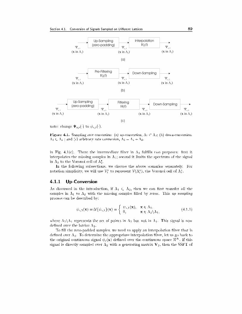
Section 4.1. Conversion of Signals Sampled on Di�erent Lattices 89
Up-Sampling
(zero-padding)
Up-Sampling
(zero-padding)
Down-Sampling
Down-Sampling
InterpolationH (f)u
FilteringH(f)
Pre-FilteringH (f)d
��
s, 1
1( in )x
��
s, 1
1( in )x
��
s, 1
1( in )x
��
s, 3
2( in )x
��
s, 3
3( in )x
��
s, 3
1( in )x
��
s, 4
3( in )x
��
s, 2
2( in )x
��
s, 2
2( in )x
��
s, 2
2( in )x
(a)
(b)
(c)
note: change s;i(�) to s;i(�).
Figure 4.1. Sampling rate conversion: (a) up-conversion, �1 � �2; (b) down-conversion,
�2 � �1 ; and (c) arbitrary rate conversion, �3 = �1 + �2.
in Fig. 4.1(c). There the intermediate �lter in �3 ful�lls two purposes: �rst it
interpolates the missing samples in �1; second it limits the spectrum of the signal
in �3 to the Voronoi cell of ��
2:
In the following subsections, we discuss the above scenarios separately. For
notation simplicity, we will use V�ito represent V(��
i), the Voronoi cell of ��
i.
4.1.1 Up-Conversion
As discussed in the introduction, if �1 � �2; then we can �rst transfer all the
samples in �1 to �2 with the missing samples �lled by zeros. This up-sampling
process can be described by:
s;3(x) = Uf s;1g(x) =
� s;1(x); x 2 �1;
0; x 2 �2n�1;(4.1.1)
where �2n�1 represents the set of points in �2 but not in �1. This signal is now
de�ned over the lattice �2.
To �ll the zero-padded samples, we need to apply an interpolation �lter that is
de�ned over �2. To determine the appropriate interpolation �lter, let us go back to
the original continuous signal c(x) de�ned over the continuous space RK: If this
signal is directly sampled over �2 with a generating matrix V2, then the SSFT of
90 Video Sampling Rate Conversion Chapter 4
the sampled signal would be
s;2(f) = d(�2)Xm2Z
K
c(f �U2m); (4.1.2)
with U2 = (VT
2 )�1: On the other hand, the SSFT of the signal sampled over �1
with a generating matrix V1 is:
s;1(f) = d(�1)Xm2ZK
c(f �U1m); (4.1.3)
with U1 = (VT
1 )�1: If �1 satis�es the alias free condition in Eq. (3.2.9), then there
will be no overlapping between the alias components in ��1.
Because �1 � �2, according to Theorem 3.3, ��1 � ��2, and consequently, V�1 �
V�2 . To derive s;2 from s;1, we just need to remove from V�2 , the portion of s;1
that is not in the original spectrum. Given that the original spectrum is not known
exactly, the best e�ort is to assume that it is the same as the portion of s;1 in
its Voronoi cell, V�1 . Therefore, the frequency response of the interpolation �lter
should be, in the ideal case:
Hu(f) =
�d(�2)=d(�1); f 2 V�1 ;
0; f 2 V�2nV�
1 :(4.1.4)
In the above equation, Hu(f) represents the SSFT of a sampled space �lter de�ned
over �2:
Example 4.1: Consider the up-conversion from the sampling lattice �1 to �2 in Fig. 4.2.
Their respective generating matrices are
V1 =
�2 1
0 1
�; V2 =
�1 0
0 1
�: (4.1.5)
Using Eq. (3.1.7), the generating matrices for the reciprocal lattices are
U1 =
�1=2 0
�1=2 1
�; U2 =
�1 0
0 1
�: (4.1.6)
The reciprocal lattices and their Voronoi cells are also shown in Fig. 4.2. Assuming the
spectrum of the original continuous signal has a circular support, we also draw in the
�gure the replicated spectra corresponding to di�erent sampling patterns. We can see
that, indeed, V�2 � V�
1 . The ideal interpolation �lter is
Hu(f) =
�d(�2)=d(�1) = 2; f 2 V�1 ;
0; f 2 V�2 nV�
1 :; (4.1.7)
as illustrated on lattice ��2 in Fig. 4.2. The �lter serves to eliminate alias components in
��1 that should not appear in ��2.
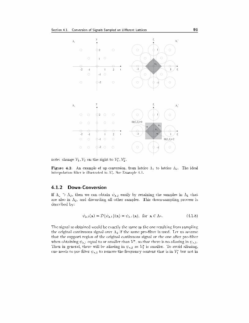
Section 4.1. Conversion of Signals Sampled on Di�erent Lattices 91
y
1 11-1
-1
1
1
2
2
-1
-1
-2
-2
t
y
1 2
2
-1
-1
-2
-2
t
ft
fy��
�� ���
���
��
1
H(f ,f )=21 2
H(f ,f )=01 2
-1
-1
1
ft
fy
��
��
note: change V1;V2 on the right to V�1 ;V�
2 .
Figure 4.2. An example of up-conversion, from lattice �1 to lattice �2. The ideal
interpolation �lter is illustrated in ��2. See Example 4.1.
4.1.2 Down-Conversion
If �1 � �2; then we can obtain s;2 easily by retaining the samples in �1 that
are also in �2, and discarding all other samples. This down-sampling process is
described by:
s;2(x) = Df s;1g(x) = s;1(x); for x 2 �2: (4.1.8)
The signal so obtained would be exactly the same as the one resulting from sampling
the original continuous signal over �2 if the same pre-�lter is used. Let us assume
that the support region of the original continuous signal or the one after pre-�lter
when obtaining s;1 equal to or smaller than V�
1 , so that there is no aliasing in s;1.
Then in general, there will be aliasing in s;2 as V�2 is smaller. To avoid aliasing,
one needs to pre-�lter s;1 to remove the frequency content that is in V�
1 but not in
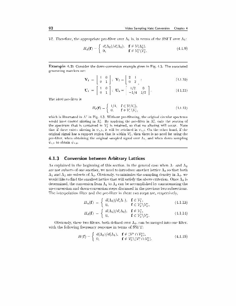
92 Video Sampling Rate Conversion Chapter 4
V�2 : Therefore, the appropriate pre-�lter over �1 is, in terms of the SSFT over �1:
Hd(f) =
�d(�2)=d(�1); f 2 V(��2);
0; f 2 V�1nV�
2 :(4.1.9)
Example 4.2: Consider the down-conversion example given in Fig. 4.3. The associated
generating matrices are:
V1 =
�1 0
0 1
�; V2 =
�2 1
0 2
�; (4.1.10)
U1 =
�1 0
0 1
�; U2 =
�1=2 0
�1=4 1=2
�: (4.1.11)
The ideal pre-�lter is
Hd(f) =
�1=4; f 2 V(��2);
0; f 2 V�1 nV�
2 ;(4.1.12)
which is illustrated in ��1 in Fig. 4.3. Without pre-�ltering, the original circular spectrum
would have caused aliasing in ��2 . By applying the pre-�lter in ��1, only the portion of
the spectrum that is contained in V�
2 is retained, so that no aliasing will occur. Note
that if there exists aliasing in s;1, it will be retained in s;2: On the other hand, if the
original signal has a support region that is within V�2 , then there is no need for using the
pre-�lter, when obtaining the original sampled signal over �1, and when down sampling
s;1 to obtain s;2.
4.1.3 Conversion between Arbitrary Lattices
As explained in the beginning of this section, in the general case when �1 and �2
are not subsets of one another, we need to introduce another lattice �3 so that both
�1 and �2 are subsets of �3: Obviously, to minimize the sampling density in �3, we
would like to �nd the smallest lattice that will satisfy the above criterion. Once �3 is
determined, the conversion from �1 to �2 can be accomplished by concatenating the
up-conversion and down-conversion steps discussed in the previous two subsections.
The interpolation �lter and the pre-�lter in these two steps are, respectively,
Hu(f) =
�d(�3)=d(�1); f 2 V�1 ;
0; f 2 V�3nV�
1 ;(4.1.13)
Hd(f) =
�d(�2)=d(�3); f 2 V�2 ;
0; f 2 V�3nV�
2 :(4.1.14)
Obviously, these two �lters, both de�ned over �3, can be merged into one �lter,
with the following frequency response in terms of SSFT:
H(f) =
�d(�2)=d(�1); f 2 (V�1 \ V�2 );
0; f 2 V�3n(V�
1 \ V�2 ):(4.1.15)
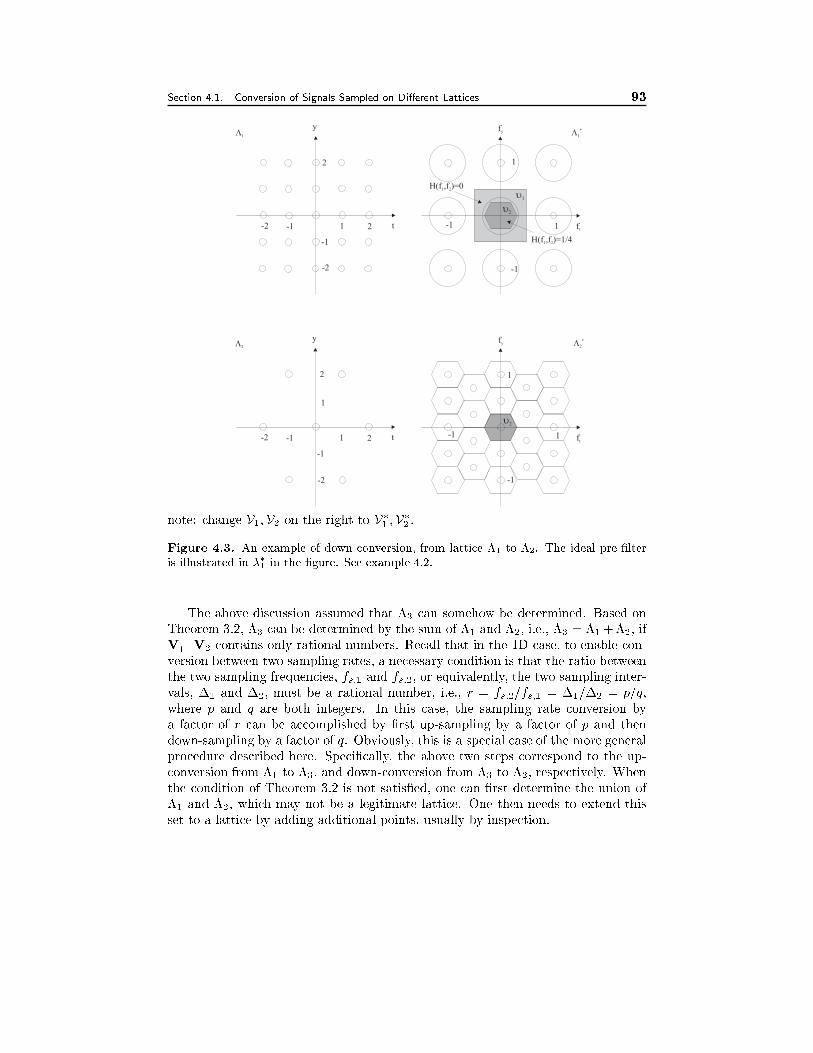
Section 4.1. Conversion of Signals Sampled on Di�erent Lattices 93
y
1 1-1
-1
1
1
2
2
-1
-1
-2
-2
t
y
1 2
2
-1
-1
-2
-2
t
ft
fy
��
�� ���
���
��
1
H(f ,f )=1/41 2
H(f ,f )=01 2
-1
-1
1
ft
fy
��
����
note: change V1;V2 on the right to V�1 ;V�
2 .
Figure 4.3. An example of down-conversion, from lattice �1 to �2. The ideal pre-�lter
is illustrated in ��1 in the �gure. See example 4.2.
The above discussion assumed that �3 can somehow be determined. Based on
Theorem 3.2, �3 can be determined by the sum of �1 and �2, i.e., �3 = �1+�2, if
V�11 V2 contains only rational numbers. Recall that in the 1D case, to enable con-
version between two sampling rates, a necessary condition is that the ratio between
the two sampling frequencies, fs;1 and fs;2, or equivalently, the two sampling inter-
vals, �1 and �2; must be a rational number, i.e., r = fs;2=fs;1 = �1=�2 = p=q;
where p and q are both integers. In this case, the sampling rate conversion by
a factor of r can be accomplished by �rst up-sampling by a factor of p and then
down-sampling by a factor of q. Obviously, this is a special case of the more general
procedure described here. Speci�cally, the above two steps correspond to the up-
conversion from �1 to �3, and down-conversion from �3 to �2, respectively. When
the condition of Theorem 3.2 is not satis�ed, one can �rst determine the union of
�1 and �2, which may not be a legitimate lattice. One then needs to extend this
set to a lattice by adding additional points, usually by inspection.
94 Video Sampling Rate Conversion Chapter 4
Example 4.3: Consider the conversion between two sampling lattices �1 and �2 with
generating matrices:
V1 =
�2 1
0 1
�; V2 =
�2 1
0 2
�: (4.1.16)
The generating matrices of their corresponding reciprocal lattices are:
U1 =
�1=2 0
�1=2 1
�; U2 =
�1=2 0
�1=4 1=2
�: (4.1.17)
First, we sketch the input and output sampling lattices �i and reciprocal lattices ��i ; i =
1; 2; based on the above generating matrices. These are illustrated in Fig. 4.4. In this case,
�1 and �2 are not subset of one another. Therefore, we need to determine a lattice �3
that is the smallest lattice that contains both �1 and �2: Because V�11 V2 includes only
rational numbers, �3 = �1+�2. In general, it is hard to determine the generating matrix
for �3 analytically. However, by visual inspection, one can see that �3 in this case must
be the square lattice sketched in Fig. 4.4. For this lattice, one obvious generating matrix
is the identity matrix, i.e.,
V3 =
�1 0
0 1
�: (4.1.18)
The reciprocal lattice is also a square lattice with the generating matrix being the identity
matrix, i.e., U3 = (VT
3 )�1 = V3:
From the sketched reciprocal lattices, ��i ; i = 1; 2; 3; we can determine their Voronoi
cells V�i individually, which are shown in Fig. 4.4. In this case, V�1 � V�
2 so that V�1 \V�
2 =
V�
2 . Therefore, the intermediate �lter should be:
H(f) =
�d(�2)
d(�1)= 1
2; f 2 V�2 ;
0; f 2 V�3 n V�
2 ;
as illustrated on top of ��3 in Fig. 4.4.
4.1.4 Filter Implementation, Design, and Other Interpolation Ap-
proaches
In the previous discussion, we have only speci�ed the desired �lter in terms of its
SSFT. The equivalent �lter in the spatial domain h(xn);xn 2 �3 can be determined
by the inverse SSFT. Theoretically, to implement the �ltering operation, we need to
�rst up-sample the input signal from �1 to �3, �lter it in �3, and then down-sample
it from �3 to �2, as shown in Fig. 4.1(c). The �ltering operation in �3 is:
s;4(xn) = s;3(xn) � h(xn) =Xym2�3
Uf s;1g(ym)h(xn � ym); xn 2 �3:(4.1.19)
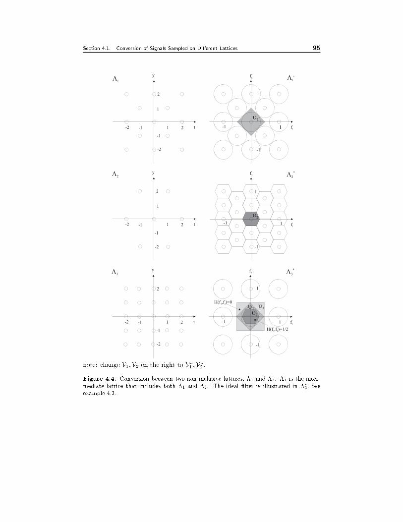
Section 4.1. Conversion of Signals Sampled on Di�erent Lattices 95
y
1
1
2
2
-1
-1
-2
-2
t
y
1 2
2
-1
-1
-2
-2
t
��
��
���
���
1-1
-1
1
ft
fy
��
��
1
H(f ,f )=1/21 2
H(f ,f )=01 2
-1
-1
1
ft
fy
������
y
1 11-1
-1
1
1
2
2
-1
-1
-2
-2
t ft
fy����
�
��
note: change V1;V2 on the right to V�1 ;V�
2 .
Figure 4.4. Conversion between two non-inclusive lattices, �1 and �2. �3 is the inter-
mediate lattice that includes both �1 and �2. The ideal �lter is illustrated in ��3: See
example 4.3.
96 Video Sampling Rate Conversion Chapter 4
In reality, the �ltering output does not have to be calculated for all the samples in
�3, as only the samples in �2 are desired in the output. In addition, because the
up-sampled input signals are non-zero only in �1, the sum in the above equation
involves only input samples in �1: Overall, the output signal over �2 can be directly
obtained from the input over �1 by
s;2(xn) = Df s;4g(xn) =Xym2�1
s;1(ym)h(xn � ym);xn 2 �2: (4.1.20)
This means that a sample xn 2 �2 is estimated by a weighted average of the samples
ym 2 �1, with weights equal to h(xn � ym):
In previous discussions, we have simply given the desired frequency responses of
the pre-�lter and reconstruction �lter, without considering how to design the �lters.
From the speci�ed frequency response H(f); f 2 V�3 , in Eq. (4.1.15), we can perform
the inverse SSFT to obtain the ideal �lter h(xn);xn 2 �3: However, this �lter will
have an in�nite extent, because the very sharp transition in H(f). If we simply
truncate the �lter, it will cause the notorious ringing artifacts in the �ltered signal.
Therefore, one needs to carefully modify the desired �lter response by applying an
appropriate windowing function, so that the corresponding �lter has a �nite extent.
One can also use various optimization techniques to directly design �nite extent
�lters so that their frequency responses are as close to the desired ones as possible.
Filter design techniques are beyond the scope of this book. Interested readers are
referred to [4], which has a good coverage on multi-dimensional �lter design. Most
of the digital �lter design techniques are developed assuming the frequency response
is speci�ed in terms of the discrete frequency. To solve the problem here, one needs
to warp the desired frequency response in terms of the continuous frequency to the
discrete frequency, as speci�ed in Eq. (3.2.16). Based on this warped frequency
response, one can apply the digital �lter design technique to derive the desired
�lter over the discrete space. One can implement the convolution operation in the
abstract discrete space, or in the sampled space directly.
As will be seen later, for video signal sampling and sampling rate conversion,
simple �lters that are far from the ideal frequency response are often used, in or-
der to reduce the computational complexity. Example �lters for several important
conversion problems are described in Sec. 4.2.
Until now, we have derived the desired interpolation �lters based on the fre-
quency domain consideration. One can also develop interpolation methods based
on sample domain requirements. For the interpolation of a continuous signal from
samples, the problem is to construct a continuous surface that passes through the
given sample values. For the up-conversion task, the problem is to estimate some
missing samples from surrounding known samples. The general approach is to use
a polynomial function with a �nite order to approximate the continuous signal over
each small region, and determine the polynomial coeÆcients based on the speci-
�ed sample values in that region using a least squares �tting procedure. Once the
polynomial is determined, one can either reconstruct the entire continuous surface,
or derive the missing samples. To maintain the continuity of the surfaces derived
Section 4.2. Sampling Rate Conversion of Video Signals 97
for adjacent regions, one can use spline functions which are special classes of the
piecewise polynomials. The most popular one being the cubic-spline approach that
has been described for 2D signal interpolation [6].
4.2 Sampling Rate Conversion of Video Signals
Sampling rate conversion is often required in video systems. For example, display of
a PAL signal on a NTSC TV system requires the conversion of an interlaced signal
with sampling rate of fs;t=50 �eld/s, fs;y=625 line/picture-height into an interlaced
signal with fs;t=60 �eld/s, fs;y=525 line/picture-height. To convert a movie on �lm
for NTSC TV broadcasting/display requires the conversion from fs;t=24 frame/s to
fs;t=60 �eld/s. Another interesting problem is to convert an interlaced raster into a
progressive one, known as deinterlacing, which is required to display a made-for-TV
material on a computer screen which uses progressive display. Some advanced TV
systems already have a built-in deinterlacing function so that interlaced material is
displayed in a progressive mode for improved visual quality.
As described in Sec. 4.1, the general procedure for solving the sampling rate
conversion problem is as follows: i) determine the equivalent sampling lattices of
the input and output signals and an intermediate lattice that covers the samples in
both input and output signals; ii) Based on the Voronoi cells of the three lattices,
determine the desired �lter frequency response; iii) Design a �lter that approxi-
mates the desired response. In reality, because of the very high data rate of the
video signal, one cannot a�ord to use a �lter with many coeÆcients, especially in
the temporal direction. To reduce the computational complexity, one can also de-
compose a spatio-temporal conversion problem into spatial conversion followed by
temporal conversion, or vice versa.
In the following, we describe the solutions for deinterlacing and for conversion
between PAL and NTSC in more detail. We will consider operations in the vertical
and temporal directions only, as the sampling rate conversion in the horizontal
direction can be done in a separate step with conventional 1D techniques. The
book by Haskell, Puri and Netravali [5] has an extensive discussion of various video
conversion problems and their practical solutions. Some of these problems are
considered in the Problem section.
4.2.1 Deinterlacing
The problem of deinterlacing is to �ll in the skipped lines in each �eld, as illustrated
in Fig. 4.5. Consider the interlaced NTSC signal, with �eld rate fs;t=60 �eld/s,
and line rate fs;y=525 line/picture-height. The sampling intervals are �t=1/60 s,
�y=1/525 picture-height. The corresponding sampling lattice and its reciprocal
are illustrated in Fig. 4.6 (a). The sampling lattice for the deinterlaced signal is
a square lattice, shown in Fig. 4.6 (b). As before, we have scaled the vertical and
temporal axes so that �y and �t are represented with the same length. Similarly,
fs;y and fs;t are assigned the same length in the frequency domain.
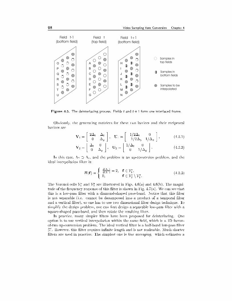
98 Video Sampling Rate Conversion Chapter 4
Field t-1
(bottom field)Field t
(top field)Field t+1
(bottom field)
Samples in
top fields
Samples in
bottom fields
Samples to be
interpolated
A
B
C
D
E
F
G
O
P
Q
R
S
T
U
H
I
J
K
L
M
N
Figure 4.5. The deinterlacing process. Fields t and t+ 1 form one interlaced frame.
Obviously, the generating matrices for these two lattices and their reciprocal
lattices are
V1 =
�2�t �t
0 �y
�; U1 =
�1=2�t 0
�1=2�y 1=�y
�; (4.2.1)
V2 =
��t 0
0 �y
�; U2 =
�1=�t 0
0 1=�y
�: (4.2.2)
In this case, �2 � �1, and the problem is an up-conversion problem, and the
ideal interpolation �lter is:
H(f) =
(d(�2)
d(�1)= 2; f 2 V�1 ;
0; f 2 V�2 n V�
1 :(4.2.3)
The Voronoi cells V�1 and V�2 are illustrated in Figs. 4.6(a) and 4.6(b). The magni-
tude of the frequency response of this �lter is shown in Fig. 4.7(a). We can see that
this is a low-pass �lter with a diamond-shaped pass-band. Notice that this �lter
is not separable (i.e. cannot be decomposed into a product of a temporal �lter
and a vertical �lter), so one has to use two dimensional �lter design technique. To
simplify the design problem, one can �rst design a separable low-pass �lter with a
square-shaped pass-band, and then rotate the resulting �lter.
In practice, many simpler �lters have been proposed for deinterlacing. One
option is to use vertical interpolation within the same �eld, which is a 1D factor-
of-two up-conversion problem. The ideal vertical �lter is a half-band low-pass �lter
[7]. However, this �lter requires in�nite length and is not realizable. Much shorter
�lters are used in practice. The simplest one is line averaging, which estimates a
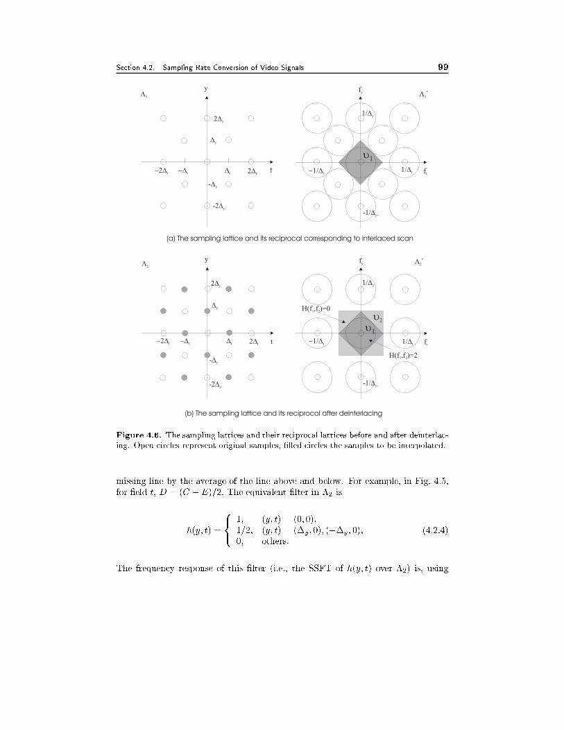
Section 4.2. Sampling Rate Conversion of Video Signals 99
y
t
��
����
�
���
H(f ,f )=21 2
H(f ,f )=01 2
ft
fy
��
��
y
2�y
2�y
-2�y-
-2�y-
�y
�y
�t
�t
�t
�t
��t
��t
��t
��t
-�y
-�y
t
��y
��y
-1/�y-
-1/�y-
��t
��t
��t
��t
ft
fy
��
(a) The sampling lattice and its reciprocal corresponding to interlaced scan
(b) The sampling lattice and its reciprocol after deinterlacing
Figure 4.6. The sampling lattices and their reciprocal lattices before and after deinterlac-
ing. Open circles represent original samples, �lled circles the samples to be interpolated.
missing line by the average of the line above and below. For example, in Fig. 4.5,
for �eld t, D = (C +E)=2: The equivalent �lter in �2 is
h(y; t) =
8<:
1; (y; t) = (0; 0);
1=2; (y; t) = (�y; 0); (��y; 0);
0; others:
(4.2.4)
The frequency response of this �lter (i.e., the SSFT of h(y; t) over �2) is, using
100 Video Sampling Rate Conversion Chapter 4
(3.2.3),
H(fy; ft) = 1 +1
2
�ej2��yfy + e
�j2��yfy�= 1 + cos(2��yfy): (4.2.5)
This frequency response is illustrated in Fig. 4.7(b). We can see that it deviates
from the desired response shown in Fig. 4.7(a) signi�cantly. Because no temporal
�ltering is applied, it has an all-pass characteristics along the temporal frequency
axis. Along the vertical frequency axis, it is far from the ideal half-band low-pass
�lter.
To improve the performance, longer vertical interpolation �lters that have fre-
quency responses closer to the ideal half-band low-pass �lter can be used. For
example, in Fig. 4.5, a satisfactory interpolation method for lines in �eld t is
D = (A + 7C + 7E + G)=16. The equivalent interpolation �lter over the dein-
terlaced grid (the vertical axis in �2) is
h = [1; 0; 7; 16; 7; 0; 1]=16: (4.2.6)
Following the same approach as before, we can easily show that the frequency
response of this �lter is
H(fy; ft) = 1 +7
8cos(2��yfy)�
1
8cos(6��yfy); (4.2.7)
which is shown in Fig. 4.7(c).
The previous two approaches use vertical interpolation only. An alternative is
to use temporal interpolation. Notice that for every missing line in a �eld, there
is a corresponding line in the other �eld of the same frame (cf. Fig. 4.5). A
simple temporal interpolation scheme is to copy this corresponding line. That is,
D = K; J = C: This method is known as �eld merging, because each deinterlaced
frame is obtained by merging two �elds. The equivalent �lter used for deinterlacing
the top �eld (assuming it appears before the bottom �eld) is:
h(y; t) =
�1; (y; t) = (0; 0); (0;��t);
0; others:(4.2.8)
The �lter for the bottom �eld is a time reversed version of the above �lter. The
frequency response of the �lter in (4.2.8) is
H(fy; ft) = 1 + e�j2��tft
: (4.2.9)
Because the �lter is asymmetric in time, it has a complex frequency response. In
addition, the temporal interpolation direction is opposite with the two �elds in
a frame. These may some times yield visual artifacts for some special patterns.
The magnitude response is illustrated in Fig. 4.7(d), which again deviates from
the desired response signi�cantly. Because �ltering is applied only in the temporal
direction, it is all-pass in the vertical direction.
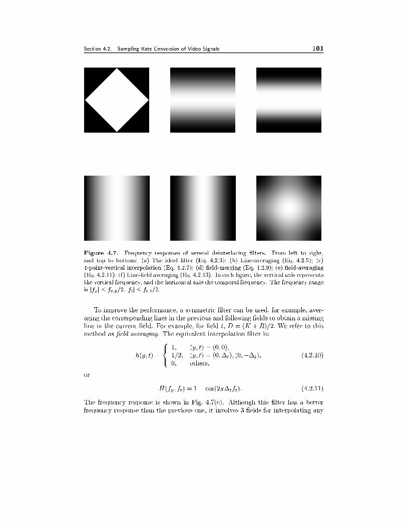
Section 4.2. Sampling Rate Conversion of Video Signals 101
Figure 4.7. Frequency responses of several deinterlacing �lters. From left to right,
and top to bottom: (a) The ideal �lter (Eq. 4.2.3); (b) Line-averaging (Eq. 4.2.5); (c)
4-point-vertical interpolation (Eq. 4.2.7); (d) �eld-merging (Eq. 4.2.9); (e) �eld-averaging
(Eq. 4.2.11); (f) Line-�eld averaging (Eq. 4.2.13). In each �gure, the vertical axis represents
the vertical frequency, and the horizontal axis the temporal frequency. The frequency range
is jfyj � fs;y=2; jftj � fs;t=2.
To improve the performance, a symmetric �lter can be used, for example, aver-
aging the corresponding lines in the previous and following �elds to obtain a missing
line in the current �eld. For example, for �eld t, D = (K + R)=2: We refer to this
method as �eld averaging. The equivalent interpolation �lter is:
h(y; t) =
8<:
1; (y; t) = (0; 0);
1=2; (y; t) = (0;�t); (0;��t);
0; others;
(4.2.10)
or
H(fy; ft) = 1 + cos(2��tft): (4.2.11)
The frequency response is shown in Fig. 4.7(e). Although this �lter has a better
frequency response than the previous one, it involves 3 �elds for interpolating any
102 Video Sampling Rate Conversion Chapter 4
�eld. This requires the storage of two frames, which represents a non-trivial increase
in memory and delay requirement compared to the previous �eld merging approach.
To achieve a compromise between spatial and temporal artifacts, a better ap-
proach is to use both vertical and temporal interpolation. For example, one can
interpolate a missing pixel by taking the average of the pixels above and below in
the same �eld, and the pixels in the previous and following �elds. In Fig. 4.5, this
corresponds to D = (C + E + K + R)=4. This method is referred to as line and
�eld averaging. The equivalent �lter on the deinterlaced lattice is:
h(y; t) =
8<:
1; (y; t) = (0; 0);
1=4; (y; t) = (�y; 0); (��y; 0); (0;�t); (0;��t);
0; others:
(4.2.12)
The frequency response is
H(fy; ft) = 1 +1
2(cos(2�fy�y) + cos(2�ft�t)) ; (4.2.13)
which is illustrated in Fig. 4.7(f). We can see that it is closer to the desired one
than all previous �lters. As with �eld averaging, this method requires the storage
of two frames. An approach that requires only one frame storage is discussed in
Problem 4.1.
When the imaged scene is stationary between adjacent �elds, the missing even
lines in an odd �eld should be exactly the same as the corresponding even lines in
the previous and following even �eld. Therefore, temporal interpolation will yield
perfect estimates. On the other hand, when there is motion in the scene, the corre-
sponding lines in adjacent �elds may not correspond to the same object location and
temporal interpolation will yield unacceptable artifacts. Imagine a vertical grating
pattern moving horizontally so that the grating pattern captured in two adjacent
�elds are shifted by half of the grating interval. Field averaging will yield serrated
vertical gratings. The methods that use both spatial and temporal averaging will
produce less severe artifacts, but the resulting video may still be unacceptable for
certain applications. For better quality, motion compensated interpolation should
be used, which is discussed in Sec. 4.2.3.
4.2.2 Conversion between NTSC and PAL Signals
In this section we consider the conversion from PAL to NTSC format signals, both
are interlaced. The conversion from NTSC to PAL will follow the same principle,
and is considered in Problem 4.4. Recall that the line and �eld rates of the PAL
signal are fy;1=625 line/picture-height and ft;1=50 �eld/s, and those for the NTSC
signal are fy;2=525 line/picture-height and ft;2=60 �eld/s. The sampling lattices
for the PAL (�1) and NTSC (�2) formats are sketched in Figs. 4.8(a) and 4.8(b), re-
spectively, where �t=1/60 s, �y=1/525 picture-height. Based on the points on each
sampling lattice, one can easily determine its generating matrix, and consequently
determine the V and U matrices. From the U matrix, one can then determine the
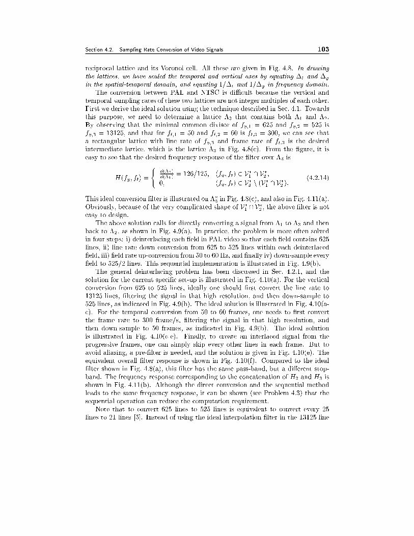
Section 4.2. Sampling Rate Conversion of Video Signals 103
reciprocal lattice and its Voronoi cell. All these are given in Fig. 4.8. In drawing
the lattices, we have scaled the temporal and vertical axes by equating �t and �y
in the spatial-temporal domain, and equating 1=�t and 1=�y in frequency domain.
The conversion between PAL and NTSC is diÆcult because the vertical and
temporal sampling rates of these two lattices are not integer multiples of each other.
First we derive the ideal solution using the technique described in Sec. 4.1. Towards
this purpose, we need to determine a lattice �3 that contains both �1 and �2:
By observing that the minimal common divisor of fy;1 = 625 and fy;2 = 525 is
fy;3 = 13125; and that for ft;1 = 50 and ft;2 = 60 is ft;3 = 300; we can see that
a rectangular lattice with line rate of fy;3 and frame rate of ft;3 is the desired
intermediate lattice, which is the lattice �3 in Fig. 4.8(c). From the �gure, it is
easy to see that the desired frequency response of the �lter over �3 is
H(fy; ft) =
(d(�2)
d(�1)= 126=125; (fy; ft) 2 V�1 \ V�2 ;
0; (fy; ft) 2 V�3 n (V�
1 \ V�2 ):(4.2.14)
This ideal conversion �lter is illustrated on ��3 in Fig. 4.8(c), and also in Fig. 4.11(a).
Obviously, because of the very complicated shape of V�1 \V�
2 , the above �lter is not
easy to design.
The above solution calls for directly converting a signal from �1 to �3 and then
back to �2, as shown in Fig. 4.9(a). In practice, the problem is more often solved
in four steps: i) deinterlacing each �eld in PAL video so that each �eld contains 625
lines, ii) line rate down conversion from 625 to 525 lines within each deinterlaced
�eld, iii) �eld rate up-conversion from 50 to 60 Hz, and �nally iv) down-sample every
�eld to 525/2 lines. This sequential implementation is illustrated in Fig. 4.9(b).
The general deinterlacing problem has been discussed in Sec. 4.2.1, and the
solution for the current speci�c set-up is illustrated in Fig. 4.10(a). For the vertical
conversion from 625 to 525 lines, ideally one should �rst convert the line rate to
13125 lines, �ltering the signal in that high resolution, and then down-sample to
525 lines, as indicated in Fig. 4.9(b). The ideal solution is illustrated in Fig. 4.10(a-
c). For the temporal conversion from 50 to 60 frames, one needs to �rst convert
the frame rate to 300 frame/s, �ltering the signal in that high resolution, and
then down-sample to 50 frames, as indicated in Fig. 4.9(b). The ideal solution
is illustrated in Fig. 4.10(c-e). Finally, to create an interlaced signal from the
progressive frames, one can simply skip every other lines in each frame. But to
avoid aliasing, a pre-�lter is needed, and the solution is given in Fig. 4.10(e). The
equivalent overall �lter response is shown in Fig. 4.10(f). Compared to the ideal
�lter shown in Fig. 4.8(a), this �lter has the same pass-band, but a di�erent stop-
band. The frequency response corresponding to the concatenation of H2 and H3 is
shown in Fig. 4.11(b). Although the direct conversion and the sequential method
leads to the same frequency response, it can be shown (see Problem 4.3) that the
sequential operation can reduce the computation requirement.
Note that to convert 625 lines to 525 lines is equivalent to convert every 25
lines to 21 lines [5]. Instead of using the ideal interpolation �lter in the 13125 line
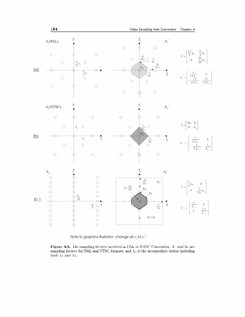
104 Video Sampling Rate Conversion Chapter 4
y
t
��(NTSC)
��(PAL)
�����
���
���
ft
fy
��
��
��
y
y
t ft
ft
fy
fy
��
��
y�25
21
t�5
6
y�42
25
t�12
5
t�
y�y�2
1
t�2
1
25
y�
5
t�
�
�
���
�
���
�
�
�
���
y
tt
V
25
210
5
6
5
12
����
�
����
�
�
��
��
yy
tU
2 1
2 5
4 2
2 5
01 2
5
�
���
�
�
���
y
ttV
0
2
����
�
����
�
�
��
��
yy
tU1
2
1
02
1
���
�
���
�
�
�
��
y
t
V
25
10
05
1
����
�
����
�
�
�
��
y
tU2 5
0
05
y�2
25
t�2
5
y�9
4
t�63
40
125
126�H
Note to graphics illustrator: change all to�i
*�i
0�H
����
(a)
(b)
(c )
Figure 4.8. The sampling lattices involved in PAL to NTSC Conversion. �1 and �2 are
sampling lattices for PAL and NTSC formats, and �3 is the intermediate lattice including
both �1 and �2.
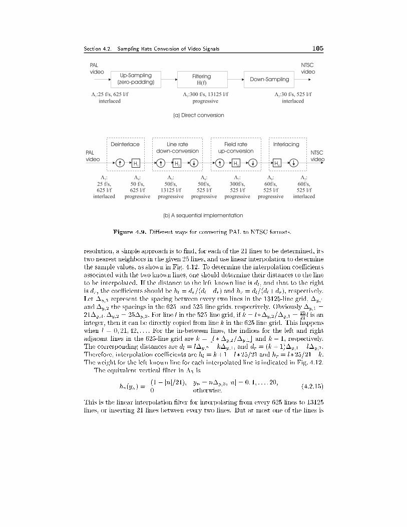
Section 4.2. Sampling Rate Conversion of Video Signals 105
PAL
video
PAL
video
NTSC
video
NTSC
video
Up-Sampling
(zero-padding)Down-Sampling
FilteringH(f)
�1:25 f/s, 625 l/f
interlaced
�1:
25 f/s,625 l/f
interlaced
�4:
50 f/s,625 l/f
progressive
�5:
50f/s,13125 l/f
progressive
�6:
50f/s,525 l/f
progressive
�7:
300f/s,525 l/f
progressive
�8:
60f/s,525 l/f
progressive
�2:
60f/s,525 l/f
interlaced
�3:300 f/s, 13125 l/f
progressive
�2:30 f/s, 525 l/f
interlaced
H1 H2 H3 H4
(a) Direct conversion
(b) A sequential implementation
Deinterlace Line rate
down-conversion
Field rate
up-conversion
Interlacing
Figure 4.9. Di�erent ways for converting PAL to NTSC formats.
resolution, a simple approach is to �nd, for each of the 21 lines to be determined, its
two nearest neighbors in the given 25 lines, and use linear interpolation to determine
the sample values, as shown in Fig. 4.12. To determine the interpolation coeÆcients
associated with the two known lines, one should determine their distances to the line
to be interpolated. If the distance to the left known line is dl, and that to the right
is dr, the coeÆcients should be hl = dr=(dl+dr) and hr = dl=(dl+dr), respectively.
Let �y;3 represent the spacing between every two lines in the 13125-line grid, �y;1
and �y;2 the spacings in the 625- and 525-line grids, respectively. Obviously �y;1 =
21�y;3;�y;2 = 25�y;3: For line l in the 525-line grid, if k = l��y;2=�y;1 =2521l is an
integer, then it can be directly copied from line k in the 625 line-grid. This happens
when l = 0; 21; 42; : : : : For the in-between lines, the indices for the left and right
adjacent lines in the 625-line grid are k = bl ��y;2=�y;1c and k + 1, respectively.
The corresponding distances are dl = l�y;2 � k�y;1; and dr = (k + 1)�y;1 � l�y;2:
Therefore, interpolation coeÆcients are hl = k+1� l�25=21 and hr = l�25=21�k:
The weight for the left known line for each interpolated line is indicated in Fig. 4.12.
The equivalent vertical �lter in �3 is
hv(yn) =(1� jnj=21); yn = n�y;3; jnj = 0; 1; : : : ; 20;
0 otherwise:(4.2.15)
This is the linear interpolation �lter for interpolating from every 625 lines to 13125
lines, or inserting 21 lines between every two lines. But at most one of the lines is
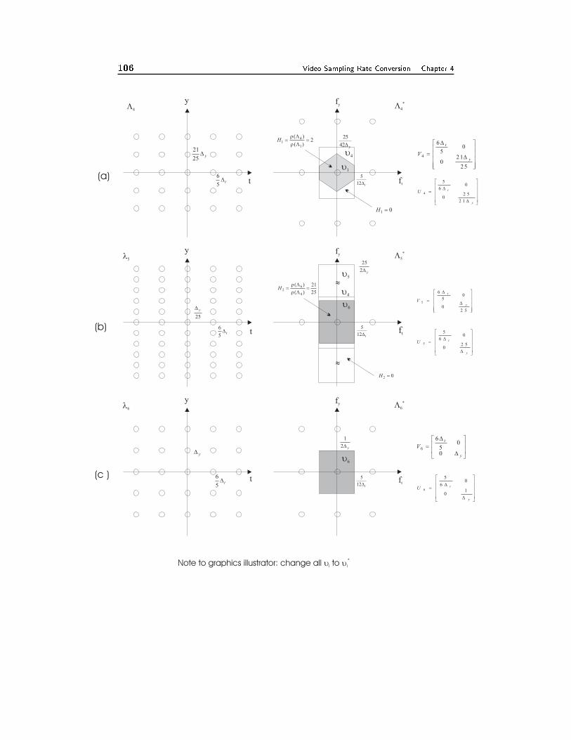
106 Video Sampling Rate Conversion Chapter 4
��
��
���
���
y
t
t
t
y
ft
ft
fy
fy
��
��
��
��
��
�� ���y
ft
fy
��
y�25
21
t�5
6
y�42
25
t�12
5
t�12
5
t�12
5
25
y�
y�y�2
1
t�5
6
t�5
6
y�2
25
2)(
)(
1
41 �
�
��
�
�H
25
21
)(
)(
4
62 �
�
��
�
�H
�
�
02 �H
01 �H
����
�
����
�
�
�
�
�
25
210
05
6
4y
t
V
����
�
����
�
�
�
�
�
2 50
05
6
5y
t
V
��
�
��
�
�
�
��
y
t
V
0
05
6
6
����
�
����
�
�
�
��
y
tU
2 1
2 50
06
5
4
����
�
����
�
�
�
��
y
tU2 5
0
06
5
5
����
�
����
�
�
�
��
y
tU1
0
06
5
6
Note to graphics illustrator: change all to�i
*�i
(a)
(b)
(c )
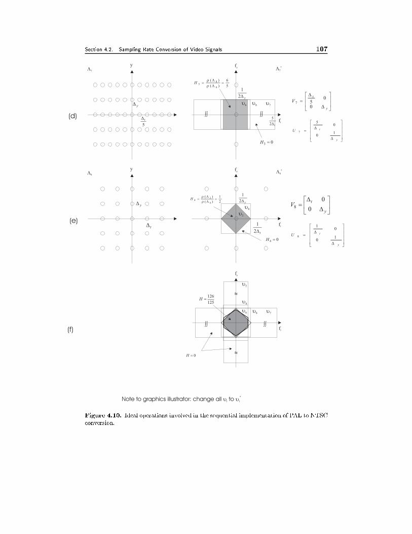
Section 4.2. Sampling Rate Conversion of Video Signals 107
��
��
���
���
y
y
ft
ft
fy
fy
��
�� ��
��
��
ft
fy
��
��
��
����
y�
5
t�
y�2
1
y�
t�
y�2
1
t�2
1
t�2
5
�
���
�
�
��
y
tV
0
08
��
�
��
�
�
�
��
y
t
V
0
057
����
�
����
�
�
�
��
y
tU1
0
01
8
����
�
����
�
�
�
��
y
tU1
0
05
7
0�H
125
126�H
5
6
)(
)(
6
83 �
��
���
H
2
1
)(
)(
8
24 �
��
���
H
04 �H
03 �H
Note to graphics illustrator: change all to�i
*�i
��
�� ��
��
�
�
(d)
(e)
(f)
Figure 4.10. Ideal operations involved in the sequential implementation of PAL to NTSC
conversion.
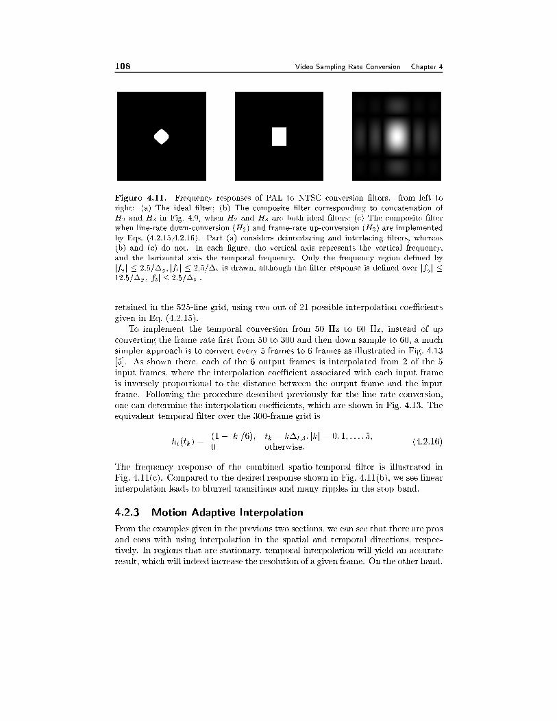
108 Video Sampling Rate Conversion Chapter 4
Figure 4.11. Frequency responses of PAL to NTSC conversion �lters. from left to
right: (a) The ideal �lter; (b) The composite �lter corresponding to concatenation of
H2 and H3 in Fig. 4.9, when H2 and H3 are both ideal �lters; (c) The composite �lter
when line-rate down-conversion (H2) and frame-rate up-conversion (H3) are implemented
by Eqs. (4.2.15,4.2.16). Part (a) considers deinterlacing and interlacing �lters, whereas
(b) and (c) do not. In each �gure, the vertical axis represents the vertical frequency,
and the horizontal axis the temporal frequency. Only the frequency region de�ned by
jfyj � 2:5=�y ; jftj � 2:5=�t is drawn, although the �lter response is de�ned over jfyj �
12:5=�y ; jftj � 2:5=�t .
retained in the 525-line grid, using two out of 21 possible interpolation coeÆcients
given in Eq. (4.2.15).
To implement the temporal conversion from 50 Hz to 60 Hz, instead of up
converting the frame rate �rst from 50 to 300 and then down sample to 60, a much
simpler approach is to convert every 5 frames to 6 frames as illustrated in Fig. 4.13
[5]. As shown there, each of the 6 output frames is interpolated from 2 of the 5
input frames, where the interpolation coeÆcient associated with each input frame
is inversely proportional to the distance between the output frame and the input
frame. Following the procedure described previously for the line rate conversion,
one can determine the interpolation coeÆcients, which are shown in Fig. 4.13. The
equivalent temporal �lter over the 300-frame grid is
ht(tk) =(1� jkj=6); tk = k�t;3; jkj = 0; 1; : : : ; 5;
0 otherwise:(4.2.16)
The frequency response of the combined spatio-temporal �lter is illustrated in
Fig. 4.11(c). Compared to the desired response shown in Fig. 4.11(b), we see linear
interpolation leads to blurred transitions and many ripples in the stop band.
4.2.3 Motion Adaptive Interpolation
From the examples given in the previous two sections, we can see that there are pros
and cons with using interpolation in the spatial and temporal directions, respec-
tively. In regions that are stationary, temporal interpolation will yield an accurate
result, which will indeed increase the resolution of a given frame. On the other hand,
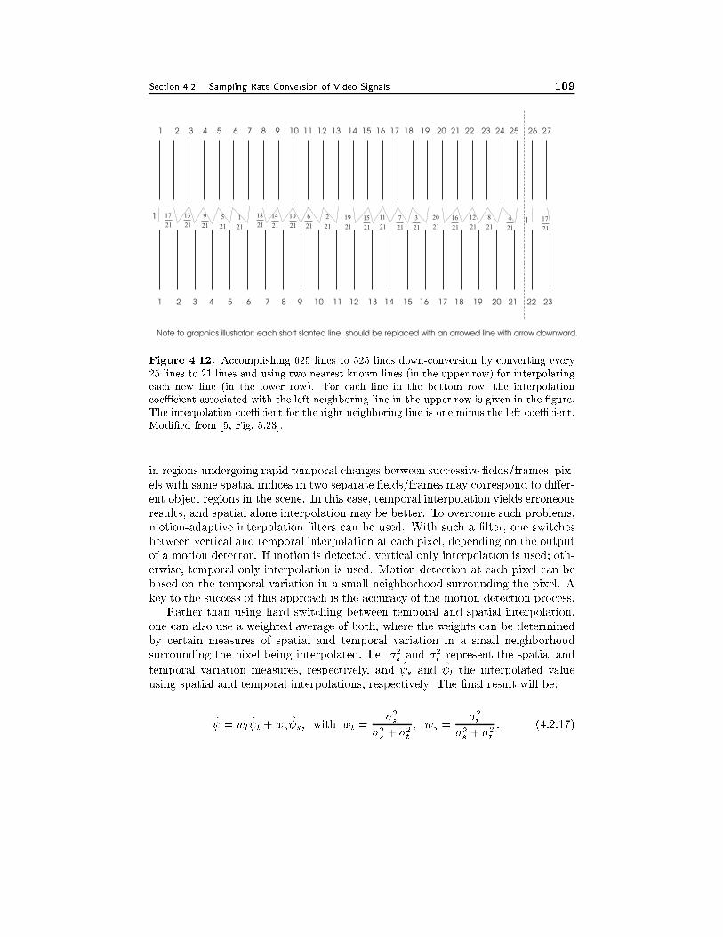
Section 4.2. Sampling Rate Conversion of Video Signals 109
1 2 3 4 5 6 7 8 9 10 11 12 13 14 15 16 17 18 19 20 21 22 23
1 2 3 4 5 6 7 8 9 10 11 12 13 14 15 16 17 18 19 20 21 22 23 24 25 26 27
11
21
17
21
1721
13
21
9
21
5
21
1
21
18
21
14
21
10
21
6
21
2
21
19
21
15
21
11
21
7
21
3
21
20
21
16
21
12
21
8
21
4
Note to graphics illustrator: each short slanted line should be replaced with an arrowed line with arrow downward.
Figure 4.12. Accomplishing 625 lines to 525 lines down-conversion by converting every
25 lines to 21 lines and using two nearest known lines (in the upper row) for interpolating
each new line (in the lower row). For each line in the bottom row, the interpolation
coeÆcient associated with the left neighboring line in the upper row is given in the �gure.
The interpolation coeÆcient for the right neighboring line is one minus the left coeÆcient.
Modi�ed from [5, Fig. 5.23].
in regions undergoing rapid temporal changes between successive �elds/frames, pix-
els with same spatial indices in two separate �elds/frames may correspond to di�er-
ent object regions in the scene. In this case, temporal interpolation yields erroneous
results, and spatial alone interpolation may be better. To overcome such problems,
motion-adaptive interpolation �lters can be used. With such a �lter, one switches
between vertical and temporal interpolation at each pixel, depending on the output
of a motion detector. If motion is detected, vertical only interpolation is used; oth-
erwise, temporal only interpolation is used. Motion detection at each pixel can be
based on the temporal variation in a small neighborhood surrounding the pixel. A
key to the success of this approach is the accuracy of the motion detection process.
Rather than using hard switching between temporal and spatial interpolation,
one can also use a weighted average of both, where the weights can be determined
by certain measures of spatial and temporal variation in a small neighborhood
surrounding the pixel being interpolated. Let �2sand �2
trepresent the spatial and
temporal variation measures, respectively, and s and t the interpolated value
using spatial and temporal interpolations, respectively. The �nal result will be:
= wt t + ws s; with wt =�2s
�2s+ �
2t
; ws =�2t
�2s+ �
2t
: (4.2.17)
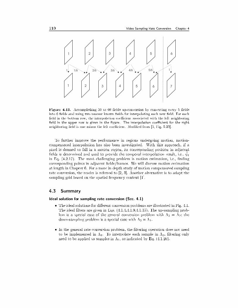
110 Video Sampling Rate Conversion Chapter 4
1 2 3 4 5 6
1 2 3 4 5 6 7
1 1/6 2/6 3/6 4/6 5/6 1
Figure 4.13. Accomplishing 50 to 60 �elds up-conversion by converting every 5 �elds
into 6 �elds and using two nearest known �elds for interpolating each new �eld. For each
�eld in the bottom row, the interpolation coeÆcient associated with the left neighboring
�eld in the upper row is given in the �gure. The interpolation coeÆcient for the right
neighboring �eld is one minus the left coeÆcient. Modi�ed from [5, Fig. 5.23].
To further improve the performance in regions undergoing motion, motion-
compensated interpolation has also been investigated. With this approach, if a
pixel is deemed to fall in a motion region, its corresponding position in adjacent
�elds is determined and used to provide the temporal interpolation result, i.e., tin Eq. (4.2.17). The most challenging problem is motion estimation, i.e., �nding
corresponding points in adjacent �elds/frames. We will discuss motion estimation
at length in Chapter 6. For a more in-depth study of motion-compensated sampling
rate conversion, the reader is referred to [2, 3]. Another alternative is to adapt the
sampling grid based on the spatial frequency content [1].
4.3 Summary
Ideal solution for sampling rate conversion (Sec. 4.1)
� The ideal solutions for di�erent conversion problems are illustrated in Fig. 4.1.
The ideal �lters are given in Eqs. (4.1.4,4.1.9,4.1.15). The up-sampling prob-
lem is a special case of the general conversion problem with �3 = �2; the
down-sampling problem is a special case with �3 = �1.
� In the general rate conversion problem, the �ltering operation does not need
to be implemented in �3. To interpolate each sample in �2, �ltering only
need to be applied to samples in �1, as indicated by Eq. (4.1.20).
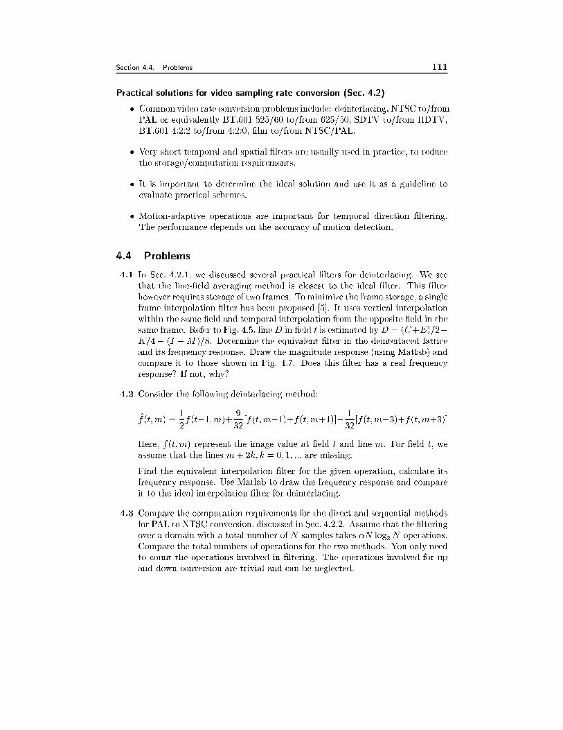
Section 4.4. Problems 111
Practical solutions for video sampling rate conversion (Sec. 4.2)
� Common video rate conversion problems include: deinterlacing, NTSC to/from
PAL or equivalently BT.601 525/60 to/from 625/50, SDTV to/from HDTV,
BT.601 4:2:2 to/from 4:2:0, �lm to/from NTSC/PAL.
� Very short temporal and spatial �lters are usually used in practice, to reduce
the storage/computation requirements.
� It is important to determine the ideal solution and use it as a guideline to
evaluate practical schemes.
� Motion-adaptive operations are important for temporal direction �ltering.
The performance depends on the accuracy of motion detection.
4.4 Problems
4.1 In Sec. 4.2.1, we discussed several practical �lters for deinterlacing. We see
that the line-�eld averaging method is closest to the ideal �lter. This �lter
however requires storage of two frames. To minimize the frame storage, a single
frame interpolation �lter has been proposed [5]. It uses vertical interpolation
within the same �eld and temporal interpolation from the opposite �eld in the
same frame. Refer to Fig. 4.5, line D in �eld t is estimated by D = (C+E)=2+
K=4� (I +M)=8. Determine the equivalent �lter in the deinterlaced lattice
and its frequency response. Draw the magnitude response (using Matlab) and
compare it to those shown in Fig. 4.7. Does this �lter has a real frequency
response? If not, why?
4.2 Consider the following deinterlacing method:
f(t;m) =1
2f(t�1;m)+
9
32[f(t;m�1)+f(t;m+1)]�
1
32[f(t;m�3)+f(t;m+3)]
Here, f(t;m) represent the image value at �eld t and line m. For �eld t, we
assume that the lines m+ 2k; k = 0; 1; ::: are missing.
Find the equivalent interpolation �lter for the given operation, calculate its
frequency response. Use Matlab to draw the frequency response and compare
it to the ideal interpolation �lter for deinterlacing.
4.3 Compare the computation requirements for the direct and sequential methods
for PAL to NTSC conversion, discussed in Sec. 4.2.2. Assume that the �ltering
over a domain with a total number of N samples takes �N log2N operations.
Compare the total numbers of operations for the two methods. You only need
to count the operations involved in �ltering. The operations involved for up
and down conversion are trivial and can be neglected.
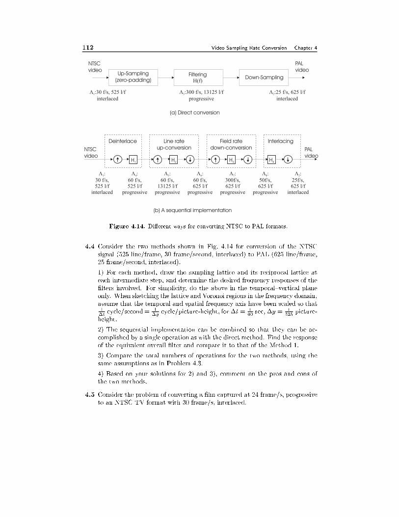
112 Video Sampling Rate Conversion Chapter 4
NTSC
video
NTSC
video
PAL
video
PAL
video
Up-Sampling
(zero-padding)Down-Sampling
FilteringH(f)
�1:30 f/s, 525 l/f
interlaced
�1:
30 f/s,525 l/f
interlaced
�4:
60 f/s,525 l/f
progressive
�5:
60 f/s,13125 l/f
progressive
�6:
60 f/s,625 l/f
progressive
�7:
300f/s,625 l/f
progressive
�8:
50f/s,625 l/f
progressive
�2:
25f/s,625 l/f
interlaced
�3:300 f/s, 13125 l/f
progressive
�2:25 f/s, 625 l/f
interlaced
H1 H2 H3 H4
(a) Direct conversion
(b) A sequential implementation
Deinterlace Line rate
up-conversion
Field rate
down-conversion
Interlacing
Figure 4.14. Di�erent ways for converting NTSC to PAL formats.
4.4 Consider the two methods shown in Fig. 4.14 for conversion of the NTSC
signal (525 line/frame, 30 frame/second, interlaced) to PAL (625 line/frame,
25 frame/second, interlaced).
1) For each method, draw the sampling lattice and its reciprocal lattice at
each intermediate step, and determine the desired frequency responses of the
�lters involved. For simplicity, do the above in the temporal{vertical plane
only. When sketching the lattice and Voronoi regions in the frequency domain,
assume that the temporal and spatial frequency axis have been scaled so that1�t
cycle/second = 1�y
cycle/picture-height, for �t = 160
sec, �y = 1525
picture-
height.
2) The sequential implementation can be combined so that they can be ac-
complished by a single operation as with the direct method. Find the response
of the equivalent overall �lter and compare it to that of the Method 1.
3) Compare the total numbers of operations for the two methods, using the
same assumptions as in Problem 4.3.
4) Based on your solutions for 2) and 3), comment on the pros and cons of
the two methods.
4.5 Consider the problem of converting a �lm captured at 24 frame/s, progressive
to an NTSC TV format with 30 frame/s, interlaced.
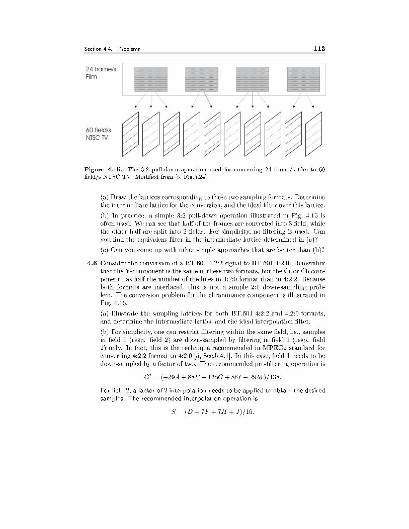
Section 4.4. Problems 113
24 frame/s
Film
60 field/s
NTSC TV
Figure 4.15. The 3:2 pull-down operation used for converting 24 frame/s �lm to 60
�eld/s NTSC TV. Modi�ed from [5, Fig.5.24]
(a) Draw the lattices corresponding to these two sampling formats. Determine
the intermediate lattice for the conversion, and the ideal �lter over this lattice.
(b) In practice, a simple 3:2 pull-down operation illustrated in Fig. 4.15 is
often used. We can see that half of the frames are converted into 3 �eld, while
the other half are split into 2 �elds. For simplicity, no �ltering is used. Can
you �nd the equivalent �lter in the intermediate lattice determined in (a)?
(c) Can you come up with other simple approaches that are better than (b)?
4.6 Consider the conversion of a BT.601 4:2:2 signal to BT.601 4:2:0. Remember
that the Y-component is the same in these two formats, but the Cr or Cb com-
ponent has half the number of the lines in 4:2:0 format than in 4:2:2. Because
both formats are interlaced, this is not a simple 2:1 down-sampling prob-
lem. The conversion problem for the chrominance component is illustrated in
Fig. 4.16.
(a) Illustrate the sampling lattices for both BT.601 4:2:2 and 4:2:0 formats,
and determine the intermediate lattice and the ideal interpolation �lter.
(b) For simplicity, one can restrict �ltering within the same �eld, i.e., samples
in �eld 1 (resp. �eld 2) are down-sampled by �ltering in �eld 1 (resp. �eld
2) only. In fact, this is the technique recommended in MPEG2 standard for
converting 4:2:2 format to 4:2:0 [5, Sec.5.4.1]. In this case, �eld 1 needs to be
down-sampled by a factor of two. The recommended pre-�ltering operation is
G0 = (�29A+ 88E + 138G+ 88I � 29M)=138:
For �eld 2, a factor of 2 interpolation needs to be applied to obtain the desired
samples. The recommended interpolation operation is
S = (D + 7F + 7H + J)=16:
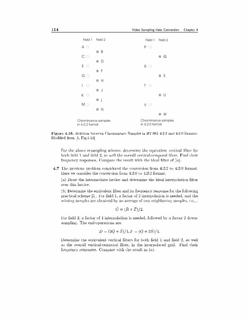
114 Video Sampling Rate Conversion Chapter 4
Field 1 Field 1Field 2 Field 2
A
C
E
G
I
B
D
F
H
J
P
R
T
Q
S
U
Chrominance samples
in 4:2:2 format
Chrominance samples
in 4:2:0 format
K
ML
N
V
W
Figure 4.16. Relation between Chrominance Samples in BT.601 4:2:2 and 4:2:0 formats.
Modi�ed from [5, Fig.5.18]
For the above resampling scheme, determine the equivalent vertical �lter for
both �eld 1 and �eld 2, as well the overall vertical-temporal �lter. Find their
frequency responses. Compare the result with the ideal �lter of (a).
4.7 The previous problem considered the conversion from 4:2:2 to 4:2:0 format.
Here we consider the conversion from 4:2:0 to 4:2:2 format.
(a) Draw the intermediate lattice and determine the ideal interpolation �lter
over this lattice.
(b) Determine the equivalent �lter and its frequency response for the following
practical scheme [5]. For �eld 1, a factor of 2 interpolation is needed, and the
missing samples are obtained by an average of two neighboring samples, i.e., ,
G = (R+ T )=2:
For �eld 2, a factor of 4 interpolation is needed, followed by a factor 2 down-
sampling. The end-operations are
D = (3Q+ S)=4; F = (Q+ 3S)=4:
Determine the equivalent vertical �lters for both �eld 1 and �eld 2, as well
as the overall vertical-temporal �lter, in the interpolated grid. Find their
frequency responses. Compare with the result in (a).
Section 4.5. Bibliography 115
4.5 Bibliography
[1] R. A. F. Belfor, M. P. A. Hesp, and R. L. Lagendijk. Spatially adaptive sub-
sampling of image sequences. IEEE Trans. Image Process., 3(5):492{500, Sept.
1994.
[2] R. A. F. Belfor, R. L. Lagendijk, and J. Biemond. Subsampling of digital image
sequences using motion information. In M. I. Sezan and R. L. Lagendijk, editors,
Motion analysis and image sequence processing, pages 189{223. Kluwer Academic
Publishers, 1993.
[3] R. A. Beuker and I. A. Shah. Analysis of interlaced video signals and its appli-
cations. IEEE Trans. Image Process., 3(5):501{512, Sept. 1994.
[4] D. E. Dudgeon and R. M. Mersereau. Multidimensional Digital Signal Process-
ing. Prentice Hall, Englewood Cli�s, NJ, 1984.
[5] B. G. Haskell, A. Puri, and A. N. Netravali. Digital Video: An Introduction to
MPEG-2. Chapman & Hall, New York, 1997.
[6] H. S. Hou and H. C. Andrews. Cubic splines for image interpolation and digital
�ltering. IEEE Trans. Acoust., Speech, Signal Processing, ASSP-26:508{517, Dec.
1978.
[7] S. K. Mitra. Digital Signal Processing - A Computer-Based Approach. McGraw
Hill, 1998.
Chapter 5
VIDEO MODELING
One of the tasks of digital video processing is to describe the change between con-secutive images of a video sequence in terms of object motion and other e�ects likeillumination changes and camera motion. In order to relate changes in the realworld to changes in a video sequence, we need parametric models describing thereal world and the image generation process. The most important models are scenemodel, object model, camera model and illumination model. These models describethe assumptions that we make about the real world. Depending on the selectedmodel, we are able to describe the real world with more or less detail and precision.Using image analysis tools, we estimate the parameters of the parametric modelsfrom the video sequence of the real world. Using the parametric models and theirestimated parameters, we can reconstruct a model world that is an approximationof the real world. Table 5.1 shows the terms that we use to name the parametricmodels, their corresponding real world entity and the entity reconstructed accordingto the parametric model and presented in the model world. We distinguish itemsof the real world from items in the model world using the pre�x real and model.When the context is clear, we may omit the pre�x.
In the following sections, we describe the camera model (Section 5.1), the illu-mination model (Section 5.2), the object model (Section 5.3), and the scene model(Section 5.4). Today, object models in most video processing applications assumeobjects with 2D motion. We present the relevant 2D motion models in Section 5.5.
Depending on the model used, the estimation of the model parameters can bediÆcult. In Chapters 6 and 7, we will discuss the estimation of the model parametersfor 2D and 3D motions, respectively.
5.1 Camera Model
The camera model describes the projection of real objects in the real scene ontothe imaging plane of the real camera. The imaging plane is also referred to as thecamera target. The image on the imaging plane is then converted into a digitalimage as described in Chapter 1.
116
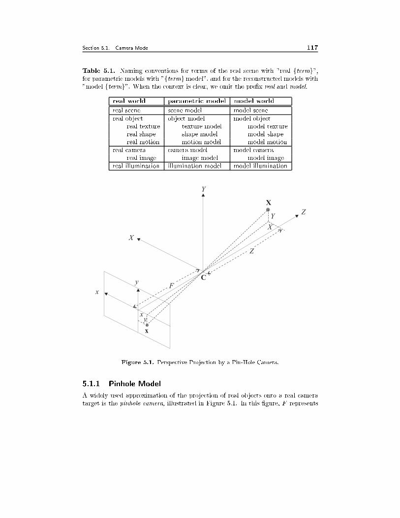
Section 5.1. Camera Model 117
Table 5.1. Naming conventions for terms of the real scene with "real ftermg",for parametric models with "ftermg model", and for the reconstructed models with"model ftermg". When the context is clear, we omit the pre�x real and model.
real world parametric model model world
real scene scene model model scene
real object object model model objectreal texture texture model model texturereal shape shape model model shapereal motion motion model model motion
real camera camera model model camerareal image image model model image
real illumination illumination model model illumination
Y
Y
X
Z
C
Z
X
X
x
x
y
x
y
F
Figure 5.1. Perspective Projection by a Pin-Hole Camera.
5.1.1 Pinhole Model
A widely used approximation of the projection of real objects onto a real cameratarget is the pinhole camera, illustrated in Figure 5.1. In this �gure, F represents
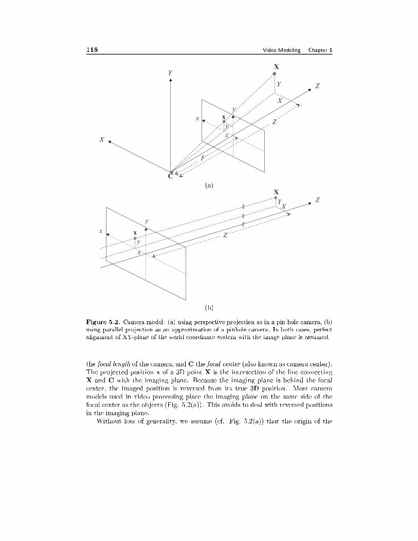
118 Video Modeling Chapter 5
Y
Y
X
Z
C
Z
X
X
x
x
y
x
y
F
(a)
Y
X
Z
Z
X
x
x
y
x
y~ ~
~ ~~ ~
(b)
Figure 5.2. Camera model: (a) using perspective projection as in a pin-hole camera, (b)
using parallel projection as an approximation of a pinhole camera. In both cases, perfect
alignment of XY-plane of the world coordinate system with the image plane is assumed.
the focal length of the camera, and C the focal center (also known as camera center).The projected position x of a 3D point X is the intersection of the line connectingX and C with the imaging plane. Because the imaging plane is behind the focalcenter, the imaged position is reversed from its true 3D position. Most cameramodels used in video processing place the imaging plane on the same side of thefocal center as the objects (Fig. 5.2(a)). This avoids to deal with reversed positionsin the imaging plane.
Without loss of generality, we assume (cf. Fig. 5.2(a)) that the origin of the
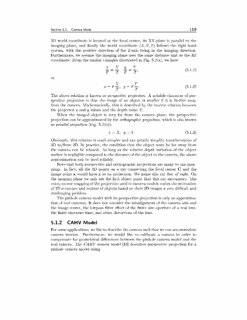
Section 5.1. Camera Model 119
3D world coordinate is located at the focal center, its XY-plane is parallel to theimaging plane, and �nally the world coordinate (X;Y; Z) follows the right-handsystem, with the positive direction of the Z-axis being in the imaging direction.Furthermore, we assume the imaging plane uses the same distance unit as the 3Dcoordinate. From the similar triangles illustrated in Fig. 5.2(a), we have
x
F=X
Z;y
F=Y
Z; (5.1.1)
or
x = FX
Z; y = F
Y
Z: (5.1.2)
The above relation is known as perspective projection. A notable character of per-spective projection is that the image of an object is smaller if it is farther awayfrom the camera. Mathematically, this is described by the inverse relation betweenthe projected x and y values and the depth value Z.
When the imaged object is very far from the camera plane, the perspectiveprojection can be approximated by the orthographic projection, which is also knownas parallel projection (Fig. 5.2(b)):
x = X; y = Y: (5.1.3)
Obviously, this relation is much simpler and can greatly simplify transformation of3D to/from 2D. In practice, the condition that the object must be far away fromthe camera can be relaxed. As long as the relative depth variation of the objectsurface is negligible compared to the distance of the object to the camera, the aboveapproximation can be used reliably.
Note that both perspective and orthographic projections are many-to-one map-pings. In fact, all the 3D points on a ray connecting the focal center C and theimage point x would have x as its projection. We name this ray line of sight. Onthe imaging plane we only see the �rst object point that this ray encounters. Themany-to-one mapping of the projection used in camera models makes the estimationof 3D structure and motion of objects based on their 2D images a very diÆcult andchallenging problem.
The pinhole camera model with its perspective projection is only an approxima-tion of real cameras. It does not consider the misalignment of the camera axis and
the image center, the lowpass �lter e�ect of the �nite size aperture of a real lens,the �nite exposure time, and other distortions of the lens.
5.1.2 CAHV Model
For some applications, we like to describe the camera such that we can accommodatecamera motion. Furthermore, we would like to calibrate a camera in order tocompensate for geometrical di�erences between the pinhole camera model and thereal camera. The CAHV camera model [16] describes perspective projection for apinhole camera model using
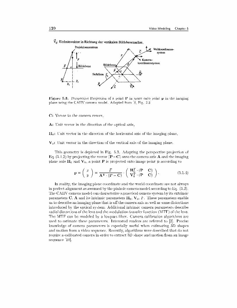
120 Video Modeling Chapter 5
Figure 5.3. Perspective Projection of a point P in space onto point p in the imaging
plane using the CAHV camera model. Adapted from [8, Fig. 2.5]
C: Vector to the camera center,
A: Unit vector in the direction of the optical axis,
H0: Unit vector in the direction of the horizontal axis of the imaging plane,
V0: Unit vector in the direction of the vertical axis of the imaging plane.
This geometry is depicted in Fig. 5.3. Adapting the perspective projection ofEq. (5.1.2) by projecting the vector (P�C) onto the camera axisA and the imagingplane axis H0 and V0, a point P is projected onto image point p according to
p =
�x
y
�=
F
AT � (P�C)�
�HT
0 � (P�C)VT
0 � (P�C)
�: (5.1.4)
In reality, the imaging plane coordinate and the world coordinate are not alwaysin perfect alignment as assumed by the pinhole camera model according to Eq. (5.2).The CAHV camera model can characterize a practical camera system by its extrinsicparameters C, A and its intrinsic parameters H0, V0, F . These parameters enableus to describe an imaging plane that is o� the camera axis as well as some distortionsintroduced by the optical system. Additional intrinsic camera parameters describeradial distortions of the lens and the modulation transfer function (MTF) of the lens.The MTF can be modeled by a lowpass �lter. Camera calibration algorithms areused to estimate these parameters. Interested readers are referred to [2]. Preciseknowledge of camera parameters is especially useful when estimating 3D shapesand motion from a video sequence. Recently, algorithms were described that do notrequire a calibrated camera in order to extract 3D shape and motion from an imagesequence [10].
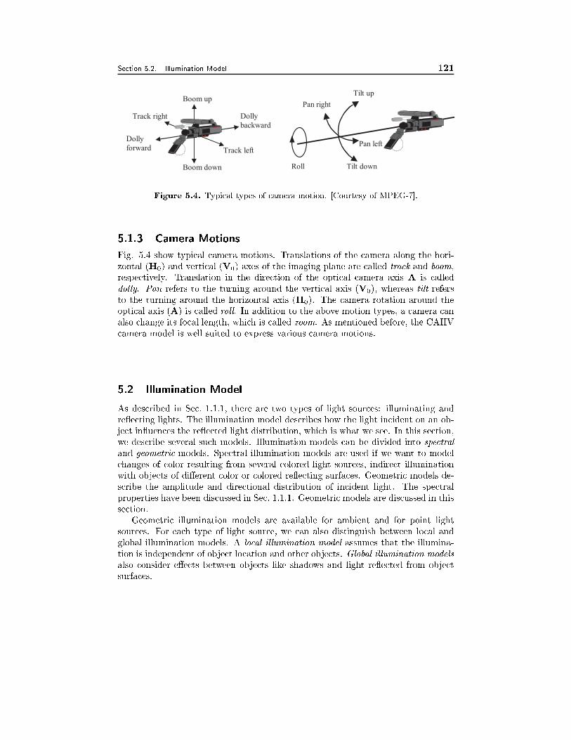
Section 5.2. Illumination Model 121
Track left
Track right
Boom up
Boom down
Dolly
backward
Dolly
forward
Pan right
Pan left
Tilt up
Tilt downRoll
Figure 5.4. Typical types of camera motion. [Courtesy of MPEG-7].
5.1.3 Camera Motions
Fig. 5.4 show typical camera motions. Translations of the camera along the hori-zontal (H0) and vertical (V0) axes of the imaging plane are called track and boom,respectively. Translation in the direction of the optical camera axis A is calleddolly. Pan refers to the turning around the vertical axis (V0), whereas tilt refersto the turning around the horizontal axis (H0). The camera rotation around theoptical axis (A) is called roll. In addition to the above motion types, a camera canalso change its focal length, which is called zoom. As mentioned before, the CAHVcamera model is well suited to express various camera motions.
5.2 Illumination Model
As described in Sec. 1.1.1, there are two types of light sources: illuminating andre ecting lights. The illumination model describes how the light incident on an ob-ject in uences the re ected light distribution, which is what we see. In this section,we describe several such models. Illumination models can be divided into spectral
and geometric models. Spectral illumination models are used if we want to modelchanges of color resulting from several colored light sources, indirect illuminationwith objects of di�erent color or colored re ecting surfaces. Geometric models de-scribe the amplitude and directional distribution of incident light. The spectralproperties have been discussed in Sec. 1.1.1. Geometric models are discussed in thissection.
Geometric illumination models are available for ambient and for point lightsources. For each type of light source, we can also distinguish between local andglobal illumination models. A local illumination model assumes that the illumina-tion is independent of object location and other objects. Global illumination models
also consider e�ects between objects like shadows and light re ected from objectsurfaces.
122 Video Modeling Chapter 5
5.2.1 Di�use and Specular Re ection
We can see only objects that re ect light and the perceived color depends on therange of wavelengths re ected. In general, the re ection can be decomposed intotwo components: the di�use re ection, which has equal energy distribution in alldirections, and the specular re ection, which is strongest in the mirror direction ofthe incident light. For a good treatment of both di�use and specular re ection, see[3]. The type of surface that exhibits only di�use re ection is known as Lambertian
surface, more commonly described as dull and matte. Wood surfaces and cementwalls belong to this category. Due to di�use re ection, we can perceive the colorof the object. Specular re ection can be observed on shiny surfaces and mirrors.Specular re ection does not show the color of the object but the color of the incidentlight. Therefore, we cannot really perceive the color of an object with a surface thatonly shows specular re ection. Except for mirrors, surfaces usually have di�use aswell as specular re ections. Only the di�use re ection determines the color of theobject surface. Looking at a human eye in daylight, we usually see the eye itselfexcept for a white spot which is caused by specular re ection of the sunlight. From
experience, we know that this spot moves on the surface if we change our positionrelative to the eye.
5.2.2 Radiance Distribution Under Di�erent Illumination and Re-
ection Conditions
In video processing, the illumination model is mainly used to describe the temporalchanges in the video sequence caused by the changing illumination of the real world.The illumination of a background may change because of an object that movestogether with its cast shadow. Since the object surface re ects light, this re ectingsource changes the overall illumination of the scene.
When discussing the interaction of a light source with an object surface, thereare three types of energy involved. First, incident ux refers to the rate at whichenergy is emitted from the light source, measured in watts (W). Second, incidentirradiance is the incident ux per unit surface area on the object and has a unit ofW/m2. Note that the irradiance at an object point depends on the angle betweenthe incident light and the surface normal at that point. Finally, re ected radiance
measures the light energy re ected from an object surface.The distribution of the re ected radiance C depends on the distribution of inci-
dent irradiance E and the object surface re ectance function r at this point. Themost general relation can be described by
C(L;V;N;X; t; �) = r(L;V;N;X; t; �) � E(L;N;X; t; �); (5.2.1)
where X is the location on the object surface, N is the surface normal vector at thelocation X, L is the illumination direction, V is the viewing direction connectingX to the focal point of the camera and � the wavelength of light (Fig. 5.5) [12].Obviously, L, V, and N are functions of X and t. The re ectance function r is
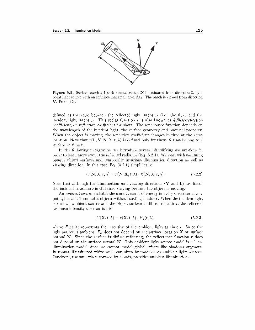
Section 5.2. Illumination Model 123
Figure 5.5. Surface patch dA with normal vector N illuminated from direction L by a
point light source with an in�nitesimal small area dAs. The patch is viewed from direction
V. From [12].
de�ned as the ratio between the re ected light intensity (i.e., the ux) and theincident light intensity. This scalar function r is also known as di�use-re ection
coeÆcient, or re ection coeÆcient for short. The re ectance function depends onthe wavelength of the incident light, the surface geometry and material property.When the object is moving, the re ection coeÆcient changes in time at the samelocation. Note that r(L;V;N;X; t; �) is de�ned only for those X that belong to asurface at time t.
In the following paragraphs, we introduce several simplifying assumptions inorder to learn more about the re ected radiance (Eq. 5.2.1). We start with assumingopaque object surfaces and temporally invariant illumination direction as well asviewing direction. In this case, Eq. (5.2.1) simpli�es to
C(N;X; t; �) = r(N;X; t; �) �E(N;X; t; �): (5.2.2)
Note that although the illumination and viewing directions (V and L) are �xed,the incident irradiance is still time varying because the object is moving.
An ambient source radiates the same amount of energy in every direction at anypoint, hence it illuminates objects without casting shadows. When the incident lightis such an ambient source and the object surface is di�use re ecting, the re ectedradiance intensity distribution is
C(X; t; �) = r(X; t; �) �Ea(t; �); (5.2.3)
where Ea(t; �) represents the intensity of the ambient light at time t. Since thelight source is ambient, Ea does not depend on the surface location X or surfacenormal N. Since the surface is di�use re ecting, the re ectance function r doesnot depend on the surface normal N. This ambient light source model is a localillumination model since we cannot model global e�ects like shadows anymore.In rooms, illuminated white walls can often be modeled as ambient light sources.Outdoors, the sun, when covered by clouds, provides ambient illumination.
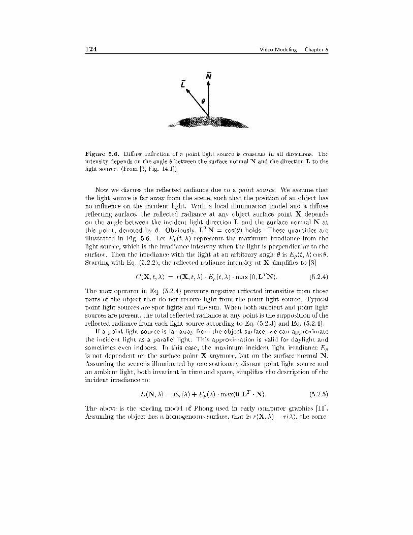
124 Video Modeling Chapter 5
Figure 5.6. Di�use re ection of a point light source is constant in all directions. The
intensity depends on the angle � between the surface normal N and the direction L to the
light source. (From [3, Fig. 14.1])
Now we discuss the re ected radiance due to a point source. We assume thatthe light source is far away from the scene, such that the position of an object hasno in uence on the incident light. With a local illumination model and a di�usere ecting surface, the re ected radiance at any object surface point X dependson the angle between the incident light direction L and the surface normal N atthis point, denoted by �. Obviously, LTN = cos(�) holds. These quantities areillustrated in Fig. 5.6. Let Ep(t; �) represents the maximum irradiance from thelight source, which is the irradiance intensity when the light is perpendicular to thesurface. Then the irradiance with the light at an arbitrary angle � is Ep(t; �) cos �.Starting with Eq. (5.2.2), the re ected radiance intensity at X simpli�es to [3]
C(X; t; �) = r(X; t; �) �Ep(t; �) �max (0;LTN): (5.2.4)
The max operator in Eq. (5.2.4) prevents negative re ected intensities from thoseparts of the object that do not receive light from the point light source. Typicalpoint light sources are spot lights and the sun. When both ambient and point lightsources are present, the total re ected radiance at any point is the supposition of there ected radiance from each light source according to Eq. (5.2.3) and Eq. (5.2.4).
If a point light source is far away from the object surface, we can approximatethe incident light as a parallel light. This approximation is valid for daylight and
sometimes even indoors. In this case, the maximum incident light irradiance Ep
is not dependent on the surface point X anymore, but on the surface normal N.
Assuming the scene is illuminated by one stationary distant point light source andan ambient light, both invariant in time and space, simpli�es the description of theincident irradiance to:
E(N; �) = Ea(�) +Ep(�) �max(0;LT �N): (5.2.5)
The above is the shading model of Phong used in early computer graphics [11].Assuming the object has a homogeneous surface, that is r(X; �) = r(�), the corre-
Section 5.2. Illumination Model 125
sponding re ected radiance becomes
C(N; �) = r(�) �E(N; �): (5.2.6)
5.2.3 Changes in the Imaged Function due to Object Motion
Now, we investigate how the illumination model can be used to describe illumina-tion e�ects in the image plane. Assuming white illumination and that the surfacenormals N and therefore the object shape are known, the illumination model inEq. (5.2.5) can be used to determine the illumination changes in an image sequencedue to object motion. Three parameters have to be estimated: the ratio betweenambient and point light irradiance Ea=Ep and the two angles describing the direc-tion L of the point light source.
The model given by Eq. (5.2.5) has been implemented in an object-based analysis-synthesis coder by Stauder [13]. In the 2D image plane, he assumes that the lumi-nance at pixel x and time t is proportional to the re ected radiance at the 3Dpoint X corresponding to x, i.e.,
(x; t) = k � C(X) = k � r(X) �E(N); (5.2.7)
where k is a constant, N denotes the normal direction corresponding to X. Thus,the luminance intensity of a point moving from xk to xk+1 (with correspondingsurface normals Nk and Nk+1), from time t to t+ dt, changes according to
(xk+1; t+ dt) = (xk ; t) �E(Nk+1)
E(Nk): (5.2.8)
Another simple illumination model assumes that the image signal (x) dependson the illumination E(x) and the re ectance function r(x), both de�ned in the imageplane. The illumination E(x) in general depends on both ambient and point lightsources. Assuming ambient illumination, di�use re ecting surfaces and a cameramodel with orthographic projection, the image signal is given by the re ection model
(x; t) = kb � E(x) � r(x; t); (5.2.9)
where kb is a constant. In the image plane, the signal (x) of a point moving fromxk to xk+1 changes according to
(xk+1; t+ dt) = kb �E(xk+1) � r(xk ; t); (5.2.10)
because r(xk+1 ; t + dt) = r(xk ; t) holds, i.e. the re ectance function moves withthe object. Equation (5.2.10) assumes that the illumination of the scene does notchange due to the motion, i.e. the object does not cast shadows in the scene. Thishas proven to be useful in 2D motion estimation using block matching, 3D motionestimation and segmentation of moving objects and their shadows [1, 4, 9, 14].
126 Video Modeling Chapter 5
The simplest and yet most widely used illumination model simply assumes thatE(x) is a constant. In this case, the luminance of a moving point does not change,and Eq. (5.2.10) simpli�es to
(xk+1; t+ dt) = (xk ; t): (5.2.11)
Sometimes, the above is referred to as constant intensity assumption. It is valid forspatially and temporally invariant ambient illumination sources and di�use re ect-ing surfaces. Under these conditions, there are no moving shadows and no re ectionsdue to glossy surfaces. Unless mentioned otherwise, the algorithms discussed in thisbook make use of this assumption.
In the above equations, we have assumed that the incident light intensity istime-invariant. However, the re ected radiance and hence the luminance image isin general space-and-time-varying, as long as the object surface is not completely at and stationary. The discussion above can be extended to the chrominance com-ponents of a video by assuming a colored incident light. Therefore, in Eqs. (5.2.7)to (5.2.11) can represent either a luminance or a color function.
5.3 Object Model
The object model describes the assumptions about real objects. Objects are entitiesin a scene that we consider to be separate items. The interpretation of what anobject might be can change depending on the application. For traÆc surveillance,we might consider each car to be an object, whereas for video coding, we mightde�ne an object according to its motion thus segmenting the car into the rotatingwheels and the translationally moving body. An object is described by a shape,motion and texture model [7].
The texture model describes the surface properties of an object. Here, we assumethat the texture of an objectm is described by the color parameters Sm. These colorparameters contain the luminance as well as the chrominance re ectance. Since weusually assume constant intensity according to Eq. (5.2.11), these color parameterscorrespond to the image signal (x).
While all object models described in this book use the same texture model, theyemploy di�erent motion and shape models as discussed in Section 5.5 and Chapter 7.Motion and shape models are usually derived from an approximate 3D descriptionof objects in order to simplify the estimation of the model parameters. Here westart with the most general shape and motion models. Simpli�cation of this modelwill be introduced as needed (Section 5.5 and Chapter 7).
5.3.1 Shape Model
The shape of a 3D object is described by the 3D space that it occupies. If we quantizethe 3D space into voxels, small cubes of edge length w, we can determine for eachvoxel whether it belongs to the object or not. This is illustrated in Fig. 5.7, where wdenotes the length of each side of the cube. Object shapes can be convex, concave or
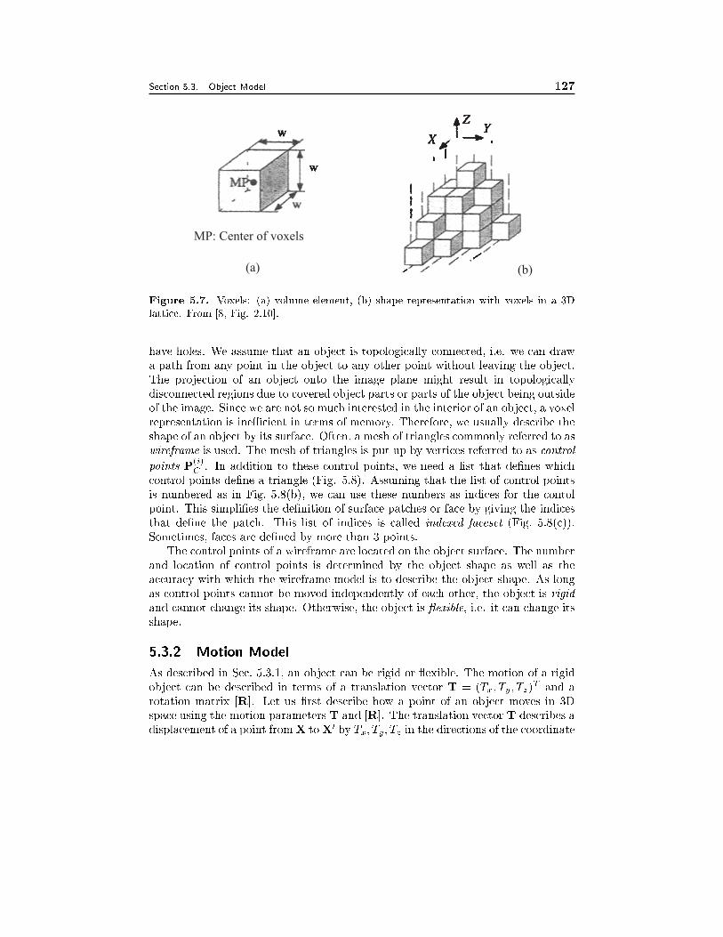
Section 5.3. Object Model 127
MP: Center of voxels
(a) (b)
Figure 5.7. Voxels: (a) volume element, (b) shape representation with voxels in a 3D
lattice. From [8, Fig. 2.10].
have holes. We assume that an object is topologically connected, i.e. we can drawa path from any point in the object to any other point without leaving the object.The projection of an object onto the image plane might result in topologicallydisconnected regions due to covered object parts or parts of the object being outsideof the image. Since we are not so much interested in the interior of an object, a voxelrepresentation is ineÆcient in terms of memory. Therefore, we usually describe theshape of an object by its surface. Often, a mesh of triangles commonly referred to aswireframe is used. The mesh of triangles is put up by vertices referred to as control
points P(i)
C . In addition to these control points, we need a list that de�nes whichcontrol points de�ne a triangle (Fig. 5.8). Assuming that the list of control pointsis numbered as in Fig. 5.8(b), we can use these numbers as indices for the contolpoint. This simpli�es the de�nition of surface patches or face by giving the indicesthat de�ne the patch. This list of indices is called indexed faceset (Fig. 5.8(c)).
Sometimes, faces are de�ned by more than 3 points.The control points of a wireframe are located on the object surface. The number
and location of control points is determined by the object shape as well as theaccuracy with which the wireframe model is to describe the object shape. As longas control points cannot be moved independently of each other, the object is rigidand cannot change its shape. Otherwise, the object is exible, i.e. it can change itsshape.
5.3.2 Motion Model
As described in Sec. 5.3.1, an object can be rigid or exible. The motion of a rigidobject can be described in terms of a translation vector T = (Tx; Ty; Tz)
T and arotation matrix [R]. Let us �rst describe how a point of an object moves in 3Dspace using the motion parameters T and [R]. The translation vector T describes adisplacement of a point fromX toX0 by Tx; Ty; Tz in the directions of the coordinate
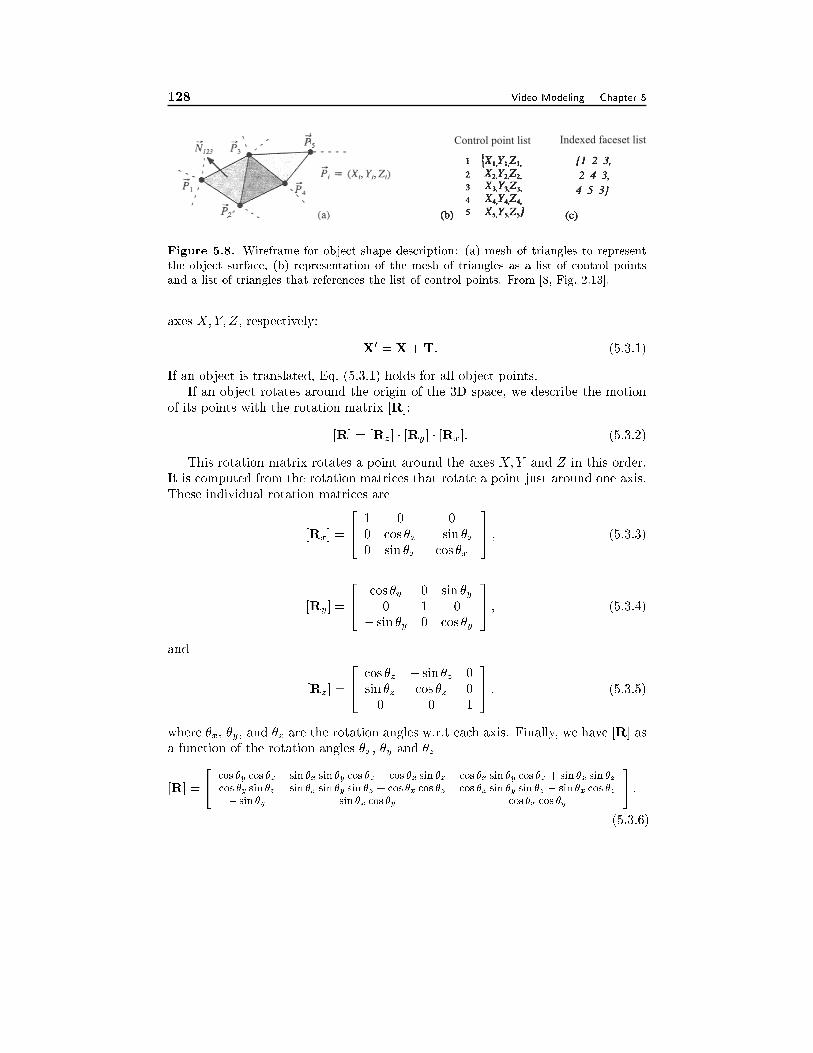
128 Video Modeling Chapter 5
Control point list Indexed faceset list
Figure 5.8. Wireframe for object shape description: (a) mesh of triangles to represent
the object surface, (b) representation of the mesh of triangles as a list of control points
and a list of triangles that references the list of control points. From [8, Fig. 2.13].
axes X;Y; Z, respectively:
X0 = X+T: (5.3.1)
If an object is translated, Eq. (5.3.1) holds for all object points.If an object rotates around the origin of the 3D space, we describe the motion
of its points with the rotation matrix [R]:
[R] = [Rz] � [Ry] � [Rx]: (5.3.2)
This rotation matrix rotates a point around the axes X;Y and Z in this order.It is computed from the rotation matrices that rotate a point just around one axis.These individual rotation matrices are
[Rx] =
24 1 0 0
0 cos �x � sin �x0 sin �x cos �x
35 ; (5.3.3)
[Ry] =
24 cos �y 0 sin �y
0 1 0� sin �y 0 cos �y
35 ; (5.3.4)
and
[Rz] =
24 cos �z � sin �z 0
sin �z cos �z 00 0 1
35 ; (5.3.5)
where �x, �y, and �z are the rotation angles w.r.t each axis. Finally, we have [R] asa function of the rotation angles �x, �y and �z
[R] =
"cos �y cos �z sin �x sin �y cos �z � cos �x sin �z cos �x sin �y cos �z + sin �x sin �zcos �y sin �z sin �x sin �y sin �z + cos �x cos �z cos �x sin �y sin �z � sin �x cos �z� sin �y sin �x cos �y cos �x cos �y
#:
(5.3.6)
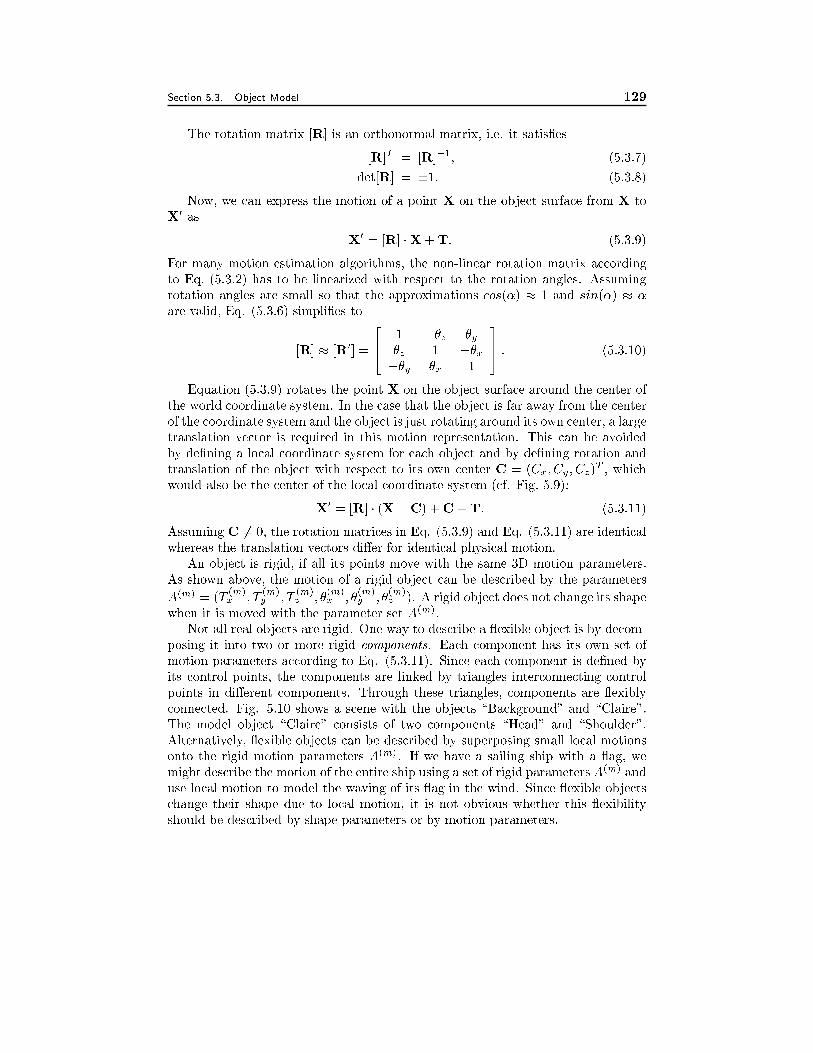
Section 5.3. Object Model 129
The rotation matrix [R] is an orthonormal matrix, i.e. it satis�es
[R]T = [R]�1; (5.3.7)
det[R] = �1: (5.3.8)
Now, we can express the motion of a point X on the object surface from X toX0 as
X0 = [R] �X+T: (5.3.9)
For many motion estimation algorithms, the non-linear rotation matrix accordingto Eq. (5.3.2) has to be linearized with respect to the rotation angles. Assumingrotation angles are small so that the approximations cos(�) � 1 and sin(�) � �
are valid, Eq. (5.3.6) simpli�es to
[R] � [R0] =
24 1 ��z �y
�z 1 ��x��y �x 1
35 : (5.3.10)
Equation (5.3.9) rotates the point X on the object surface around the center ofthe world coordinate system. In the case that the object is far away from the centerof the coordinate system and the object is just rotating around its own center, a largetranslation vector is required in this motion representation. This can be avoidedby de�ning a local coordinate system for each object and by de�ning rotation andtranslation of the object with respect to its own center C = (Cx; Cy; Cz)
T , whichwould also be the center of the local coordinate system (cf. Fig. 5.9):
X0 = [R] � (X�C) +C+T: (5.3.11)
Assuming C 6= 0, the rotation matrices in Eq. (5.3.9) and Eq. (5.3.11) are identicalwhereas the translation vectors di�er for identical physical motion.
An object is rigid, if all its points move with the same 3D motion parameters.As shown above, the motion of a rigid object can be described by the parameters
A(m) = (T(m)x ; T
(m)y ; T
(m)z ; �
(m)x ; �
(m)y ; �
(m)z ). A rigid object does not change its shape
when it is moved with the parameter set A(m).Not all real objects are rigid. One way to describe a exible object is by decom-
posing it into two or more rigid components. Each component has its own set ofmotion parameters according to Eq. (5.3.11). Since each component is de�ned byits control points, the components are linked by triangles interconnecting controlpoints in di�erent components. Through these triangles, components are exiblyconnected. Fig. 5.10 shows a scene with the objects \Background" and \Claire".The model object \Claire" consists of two components \Head" and \Shoulder".Alternatively, exible objects can be described by superposing small local motionsonto the rigid motion parameters A(m). If we have a sailing ship with a ag, wemight describe the motion of the entire ship using a set of rigid parameters A(m) anduse local motion to model the waving of its ag in the wind. Since exible objectschange their shape due to local motion, it is not obvious whether this exibilityshould be described by shape parameters or by motion parameters.
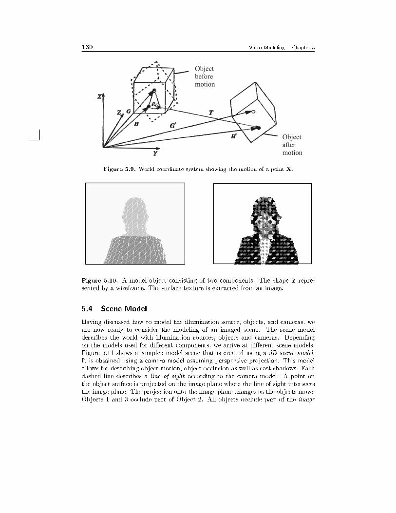
130 Video Modeling Chapter 5
Objectbeforemotion
Objectaftermotion
Figure 5.9. World coordinate system showing the motion of a point X.
Figure 5.10. A model object consisting of two components. The shape is repre-sented by a wireframe. The surface texture is extracted from an image.
5.4 Scene Model
Having discussed how to model the illumination source, objects, and cameras, weare now ready to consider the modeling of an imaged scene. The scene modeldescribes the world with illumination sources, objects and cameras. Dependingon the models used for di�erent components, we arrive at di�erent scene models.Figure 5.11 shows a complex model scene that is created using a 3D scene model.It is obtained using a camera model assuming perspective projection. This modelallows for describing object motion, object occlusion as well as cast shadows. Eachdashed line describes a line of sight according to the camera model. A point onthe object surface is projected on the image plane where the line of sight intersectsthe image plane. The projection onto the image plane changes as the objects move.Objects 1 and 3 occlude part of Object 2. All objects occlude part of the image
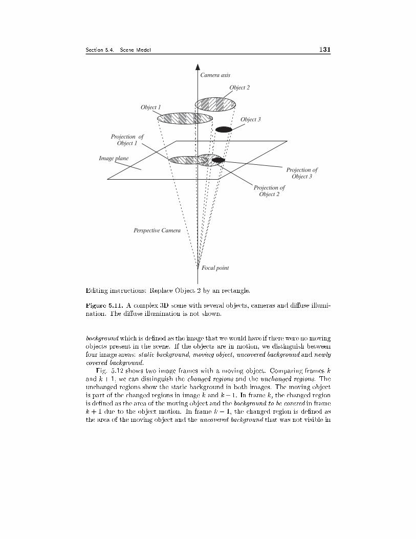
Section 5.4. Scene Model 131
Editing instructions: Replace Object 2 by an rectangle.
Figure 5.11. A complex 3D scene with several objects, cameras and di�use illumi-nation. The di�use illumination is not shown.
background which is de�ned as the image that we would have if there were no movingobjects present in the scene. If the objects are in motion, we distinguish betweenfour image areas: static background, moving object, uncovered background and newlycovered background.
Fig. 5.12 shows two image frames with a moving object. Comparing frames kand k + 1, we can distinguish the changed regions and the unchanged regions. Theunchanged regions show the static background in both images. The moving objectis part of the changed regions in image k and k+1. In frame k, the changed regionis de�ned as the area of the moving object and the background to be covered in framek + 1 due to the object motion. In frame k + 1, the changed region is de�ned asthe area of the moving object and the uncovered background that was not visible in
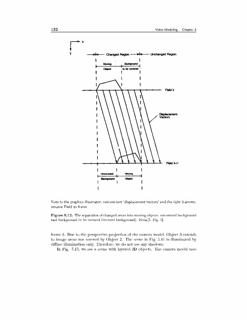
132 Video Modeling Chapter 5
Note to the graphics illustrator: remove text 'displacement vectors' and the right 3 arrows,
rename Field to frame
Figure 5.12. The separation of changed areas into moving objects, uncovered background
and background to be covered (covered background). From[5, Fig. 5].
frame k. Due to the perspective projection of the camera model, Object 3 extendsto image areas not covered by Object 2. The scene in Fig. 5.11 is illuminated bydi�use illumination only. Therefore, we do not see any shadows.
In Fig. 5.13, we see a scene with layered 2D objects. The camera model uses
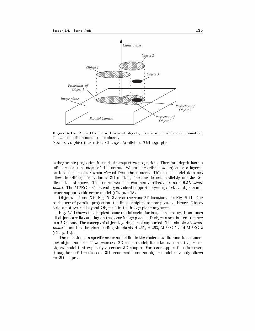
Section 5.4. Scene Model 133
Figure 5.13. A 2.5 D scene with several objects, a camera and ambient illumination.
The ambient illumination is not shown.
Note to graphics illustrator: Change 'Parallel' to 'Orthographic'
orthographic projection instead of perspective projection. Therefore depth has noin uence on the image of this scene. We can describe how objects are layeredon top of each other when viewed from the camera. This scene model does notallow describing e�ects due to 3D motion, since we do not explicitly use the 3rddimension of space. This scene model is commonly referred to as a 2.5D scene
model. The MPEG-4 video coding standard supports layering of video objects andhence supports this scene model (Chapter 13).
Objects 1, 2 and 3 in Fig. 5.13 are at the same 3D location as in Fig. 5.11. Dueto the use of parallel projection, the lines of sight are now parallel. Hence, Object3 does not extend beyond Object 2 in the image plane anymore.
Fig. 5.14 shows the simplest scene model useful for image processing. It assumesall objects are at and lay on the same image plane. 2D objects are limited to movein a 2D plane. The concept of object layering is not supported. This simple 2D scene
model is used in the video coding standards H.261, H.263, MPEG-1 and MPEG-2(Chap. 13).
The selection of a speci�c scene model limits the choices for illumination, cameraand object models. If we choose a 2D scene model, it makes no sense to pick anobject model that explicitly describes 3D shapes. For some applications however,it may be useful to choose a 3D scene model and an object model that only allowsfor 2D shapes.
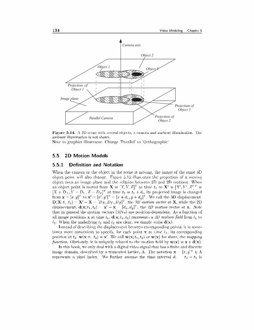
134 Video Modeling Chapter 5
Figure 5.14. A 2D scene with several objects, a camera and ambient illumination. The
ambient illumination is not shown.
Note to graphics illustrator: Change 'Parallel' to 'Orthographic'
5.5 2D Motion Models
5.5.1 De�nition and Notation
When the camera or the object in the scene is moving, the image of the same 3Dobject point will also change. Figure 5.15 illustrates the projection of a movingobject onto an image plane and the relation between 3D and 2D motions. Whenan object point is moved from X = [X;Y; Z]T at time t1 to X0 = [X 0; Y 0; Z 0]T =[X +DX ; Y +DY ; Z +DZ ]
T at time t2 = t1 + dt, its projected image is changedfrom x = [x; y]T to x0 = [x0; y0]T = [x+ dx; y + dy ]
T . We call the 3D displacement,D(X; t1; t2) = X0 �X = [DX ; DY ; DZ ]
T , the 3D motion vector at X, while the 2Ddisplacement, d(x; t1; t2) = x0 � x = [dx; dy]
T , the 2D motion vector at x. Notethat in general the motion vectors (MVs) are position-dependent. As a function ofall image positions x at time t1, d(x; t1; t2) represents a 2D motion �eld from t1 tot2. When the underlying t1 and t2 are clear, we simply write d(x).
Instead of describing the displacement between corresponding points, it is some-times more convenient to specify, for each point x at time t1, its correspondingposition at t2, w(x; t1; t2) = x0. We call w(x; t1; t2) or w(x) for short, the mapping
function. Obviously, it is uniquely related to the motion �eld by w(x) = x+ d(x).In this book, we only deal with a digital video signal that has a �nite and discrete
image domain, described by a truncated lattice, �. The notation x = [x; y]T 2 �represents a pixel index. We further assume the time interval dt = t2 � t1 is
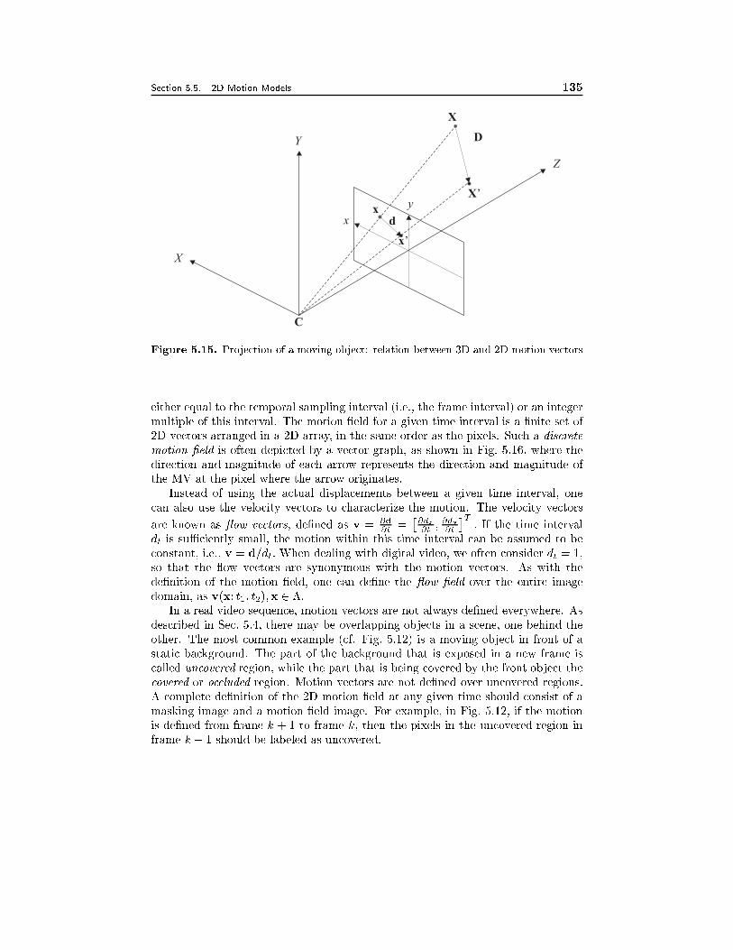
Section 5.5. 2D Motion Models 135
Y
X
D
X’
Z
C
X
x
yx
d
x’
Figure 5.15. Projection of a moving object: relation between 3D and 2D motion vectors
either equal to the temporal sampling interval (i.e., the frame interval) or an integermultiple of this interval. The motion �eld for a given time interval is a �nite set of2D vectors arranged in a 2D array, in the same order as the pixels. Such a discrete
motion �eld is often depicted by a vector graph, as shown in Fig. 5.16, where thedirection and magnitude of each arrow represents the direction and magnitude ofthe MV at the pixel where the arrow originates.
Instead of using the actual displacements between a given time interval, onecan also use the velocity vectors to characterize the motion. The velocity vectors
are known as ow vectors, de�ned as v = @d@t
=�@dx@t; @dx@t
�T: If the time interval
dt is suÆciently small, the motion within this time interval can be assumed to beconstant, i.e., v = d=dt: When dealing with digital video, we often consider dt = 1,so that the ow vectors are synonymous with the motion vectors. As with thede�nition of the motion �eld, one can de�ne the ow �eld over the entire imagedomain, as v(x; t1; t2);x 2 �:
In a real video sequence, motion vectors are not always de�ned everywhere. Asdescribed in Sec. 5.4, there may be overlapping objects in a scene, one behind theother. The most common example (cf. Fig. 5.12) is a moving object in front of astatic background. The part of the background that is exposed in a new frame iscalled uncovered region, while the part that is being covered by the front object thecovered or occluded region. Motion vectors are not de�ned over uncovered regions.A complete de�nition of the 2D motion �eld at any given time should consist of amasking image and a motion �eld image. For example, in Fig. 5.12, if the motionis de�ned from frame k + 1 to frame k, then the pixels in the uncovered region inframe k + 1 should be labeled as uncovered.
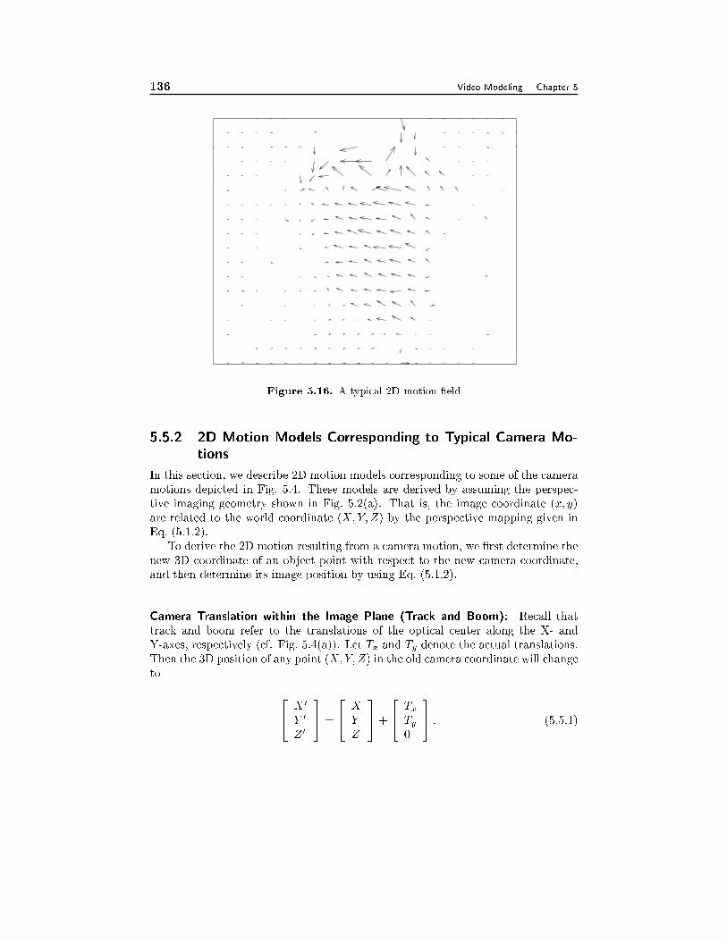
136 Video Modeling Chapter 5
Figure 5.16. A typical 2D motion �eld
5.5.2 2D Motion Models Corresponding to Typical Camera Mo-
tions
In this section, we describe 2D motion models corresponding to some of the cameramotions depicted in Fig. 5.4. These models are derived by assuming the perspec-tive imaging geometry shown in Fig. 5.2(a). That is, the image coordinate (x; y)are related to the world coordinate (X;Y; Z) by the perspective mapping given inEq. (5.1.2).
To derive the 2D motion resulting from a camera motion, we �rst determine thenew 3D coordinate of an object point with respect to the new camera coordinate,and then determine its image position by using Eq. (5.1.2).
Camera Translation within the Image Plane (Track and Boom): Recall thattrack and boom refer to the translations of the optical center along the X- andY-axes, respectively (cf. Fig. 5.4(a)). Let Tx and Ty denote the actual translations.Then the 3D position of any point (X;Y; Z) in the old camera coordinate will changeto
24 X 0
Y 0
Z 0
35 =
24 X
Y
Z
35+
24 TxTy0
35 : (5.5.1)
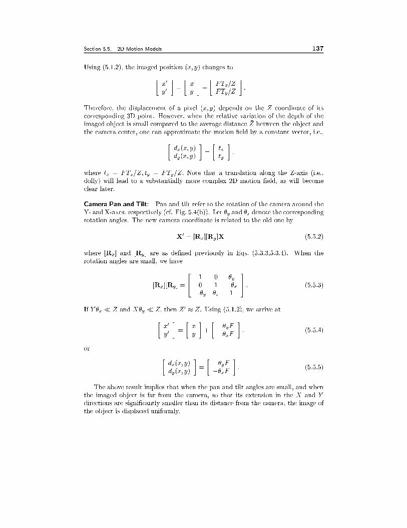
Section 5.5. 2D Motion Models 137
Using (5.1.2), the imaged position (x; y) changes to
�x0
y0
�=
�x
y
�+
�FTx=Z
FTy=Z
�:
Therefore, the displacement of a pixel (x; y) depends on the Z coordinate of itscorresponding 3D point. However, when the relative variation of the depth of theimaged object is small compared to the average distance �Z between the object andthe camera center, one can approximate the motion �eld by a constant vector, i.e.,
�dx(x; y)dy(x; y)
�=
�txty
�;
where tx = FTx= �Z; ty = FTy= �Z: Note that a translation along the Z-axis (i.e.,dolly) will lead to a substantially more complex 2D motion �eld, as will becomeclear later.
Camera Pan and Tilt: Pan and tilt refer to the rotation of the camera around theY- and X-axes, respectively (cf. Fig. 5.4(b)). Let �y and �x denote the corresponding
rotation angles. The new camera coordinate is related to the old one by
X0 = [Rx][Ry]X (5.5.2)
where [Rx] and [Ry] are as de�ned previously in Eqs. (5.3.3,5.3.4). When therotation angles are small, we have
[Rx][Ry] =
24 1 0 �y
0 1 ��x��y �x 1
35 : (5.5.3)
If Y �x � Z and X�y � Z; then Z 0 � Z. Using (5.1.2), we arrive at
�x0
y0
�=
�x
y
�+
��yF
��xF
�: (5.5.4)
or �dx(x; y)dy(x; y)
�=
��yF
��xF
�: (5.5.5)
The above result implies that when the pan and tilt angles are small, and whenthe imaged object is far from the camera, so that its extension in the X and Y
directions are signi�cantly smaller than its distance from the camera, the image ofthe object is displaced uniformly.
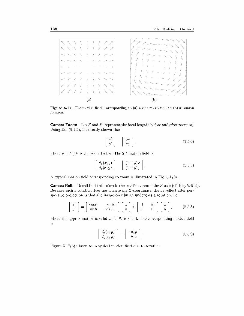
138 Video Modeling Chapter 5
(a) (b)
Figure 5.17. The motion �elds corresponding to (a) a camera zoom; and (b) a camera
rotation.
Camera Zoom: Let F and F 0 represent the focal lengths before and after zooming.Using Eq. (5.1.2), it is easily shown that
�x0
y0
�=
��x
�y
�; (5.5.6)
where � = F 0=F is the zoom factor. The 2D motion �eld is
�dx(x; y)dy(x; y)
�=
�(1� �)x(1� �)y
�: (5.5.7)
A typical motion �eld corresponding to zoom is illustrated in Fig. 5.17(a).
Camera Roll: Recall that this refers to the rotation around the Z-axis (cf. Fig. 5.4(b)).Because such a rotation does not change the Z-coordinate, the net-e�ect after per-spective projection is that the image coordinate undergoes a rotation, i.e.,
�x0
y0
�=
�cos �z � sin �zsin �z cos �z
� �x
y
��
�1 ��z�z 1
��x
y
�; (5.5.8)
where the approximation is valid when �z is small. The corresponding motion �eldis �
dx(x; y)dy(x; y)
�=
���zy�zx
�: (5.5.9)
Figure 5.17(b) illustrates a typical motion �eld due to rotation.
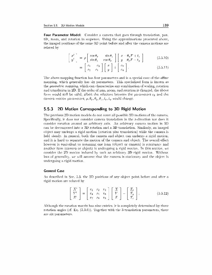
Section 5.5. 2D Motion Models 139
Four Parameter Model: Consider a camera that goes through translation, pan,tilt, zoom, and rotation in sequence. Using the approximations presented above,the imaged positions of the same 3D point before and after the camera motions arerelated by
�x0
y0
�= �
�cos �z � sin �zsin �z cos �z
��x+ �yF + txy � �xF + ty
�(5.5.10)
=
�c1 �c2c2 c1
� �x
y
�+
�c3c4
�: (5.5.11)
The above mapping function has four parameters and is a special case of the aÆnemapping, which generally has six parameters. This specialized form is known asthe geometric mapping, which can characterize any combination of scaling, rotationand translation in 2D. If the order of pan, zoom, and rotation is changed, the aboveform would still be valid, albeit the relations between the parameters ck and the
camera motion parameters, �; �x; �y; �z; tx; ty would change.
5.5.3 2D Motion Corresponding to 3D Rigid Motion
The previous 2D motion models do not cover all possible 3D motions of the camera.
Speci�cally, it does not consider camera translation in the z-direction nor does itconsider rotation around an arbitrary axis. An arbitrary camera motion in 3Dcan be decomposed into a 3D rotation and a 3D translation. Similarly, an imagedobject may undergo a rigid motion (rotation plus translation) while the camera isheld steady. In general, both the camera and object can undergo a rigid motion,and it is hard to separate the motion of the camera and object. The overall e�ecthowever is equivalent to assuming one item (object or camera) is stationary andanother item (camera or object) is undergoing a rigid motion. In this section, weconsider the 2D motion induced by such an arbitrary 3D rigid motion. Withoutloss of generality, we will assume that the camera is stationary and the object isundergoing a rigid motion.
General Case
As described in Sec. 5.3, the 3D positions of any object point before and after arigid motion are related by
24 X 0
Y 0
Z 0
35 =
24 r1 r2 r3r4 r5 r6r7 r8 r9
3524 X
Y
Z
35+
24 TxTyTz
35 : (5.5.12)
Although the rotation matrix has nine entries, it is completely determined by threerotation angles (cf. Eq. (5.3.6)). Together with the 3 translation parameters, thereare six parameters.
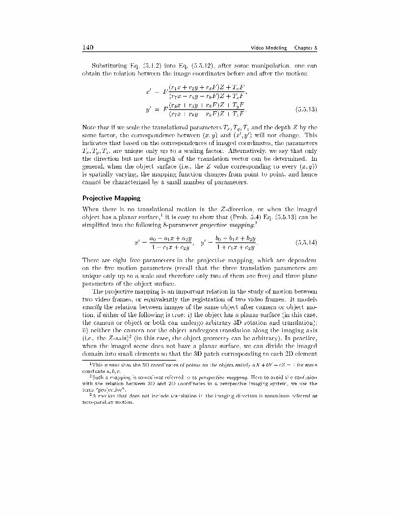
140 Video Modeling Chapter 5
Substituting Eq. (5.1.2) into Eq. (5.5.12), after some manipulation, one canobtain the relation between the image coordinates before and after the motion:
x0 = F(r1x+ r2y + r3F )Z + TxF
(r7x+ r8y + r9F )Z + TzF;
y0 = F(r4x+ r5y + r6F )Z + TyF
(r7x+ r8y + r9F )Z + TzF: (5.5.13)
Note that if we scale the translational parameters Tx; Ty; Tz and the depth Z by thesame factor, the correspondence between (x; y) and (x0; y0) will not change. Thisindicates that based on the correspondences of imaged coordinates, the parametersTx; Ty; Tz; are unique only up to a scaling factor. Alternatively, we say that onlythe direction but not the length of the translation vector can be determined. Ingeneral, when the object surface (i.e., the Z value corresponding to every (x; y))is spatially varying, the mapping function changes from point to point, and hence
cannot be characterized by a small number of parameters.
Projective Mapping
When there is no translational motion in the Z-direction, or when the imagedobject has a planar surface,1 it is easy to show that (Prob. 5.4) Eq. (5.5.13) can besimpli�ed into the following 8-parameter projective mapping:2
x0 =a0 + a1x+ a2y
1 + c1x+ c2y; y0 =
b0 + b1x+ b2y
1 + c1x+ c2y: (5.5.14)
There are eight free parameters in the projective mapping, which are dependenton the �ve motion parameters (recall that the three translation parameters areunique only up to a scale and therefore only two of them are free) and three planeparameters of the object surface.
The projective mapping is an important relation in the study of motion betweentwo video frames, or equivalently the registration of two video frames. It modelsexactly the relation between images of the same object after camera or object mo-tion, if either of the following is true: i) the object has a planar surface (in this case,the camera or object or both can undergo arbitrary 3D rotation and translation);ii) neither the camera nor the object undergoes translation along the imaging axis(i.e., the Z-axis)3 (in this case, the object geometry can be arbitrary). In practice,when the imaged scene does not have a planar surface, we can divide the imageddomain into small elements so that the 3D patch corresponding to each 2D element
1This means that the 3D coordinates of points on the object satisfy aX+bY +cZ = 1 for some
constants a; b; c:2Such a mapping is sometimes referred to as perspective mapping. Here to avoid the confusion
with the relation between 3D and 2D coordinates in a perspective imaging system, we use the
term \projective".3A motion that does not include translation in the imaging direction is sometimes referred as
zero-parallax motion.
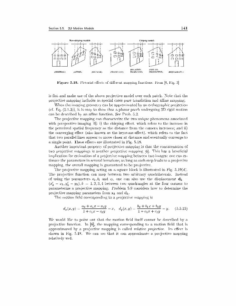
Section 5.5. 2D Motion Models 141
Figure 5.18. Pictorial e�ects of di�erent mapping functions. From [6, Fig. 3]
is at and make use of the above projective model over each patch. Note that theprojective mapping includes as special cases pure translation and aÆne mapping.
When the imaging geometry can be approximated by an orthographic projection(cf. Eq. (5.1.3)), it is easy to show that a planar patch undergoing 3D rigid motioncan be described by an aÆne function. See Prob. 5.2.
The projective mapping can characterize the two unique phenomena associatedwith perspective imaging [6]: i) the chirping e�ect, which refers to the increase inthe perceived spatial frequency as the distance from the camera increases; and ii)the converging e�ect (also known as the keystone e�ect), which refers to the factthat two parallel lines appear to move closer at distance and eventually converge toa single point. These e�ects are illustrated in Fig. 5.18.
Another important property of projective mapping is that the concatenation oftwo projective mappings is another projective mapping [6]. This has a bene�cialimplication for estimation of a projective mapping between two images: one can es-timate the parameters in several iterations; as long as each step leads to a projectivemapping, the overall mapping is guaranteed to be projective.
The projective mapping acting on a square block is illustrated in Fig. 5.19(d).The projective function can map between two arbitrary quadrilaterals. Insteadof using the parameters al; bl and cl, one can also use the displacement dk =(x0k � xk; y
0
k � yk); k = 1; 2; 3; 4 between two quadrangles at the four corners toparameterize a projective mapping. Problem 5.9 considers how to determine theprojective mapping parameters from xk and dk.
The motion �eld corresponding to a projective mapping is
dx(x; y) =a0 + a1x+ a2y
1 + c1x+ c2y� x; dy(x; y) =
b0 + b1x+ b2y
1 + c1x+ c2y� y: (5.5.15)
We would like to point out that the motion �eld itself cannot be described by aprojective function. In [6], the mapping corresponding to a motion �eld that isapproximated by a projective mapping is called relative projective. Its e�ect isshown in Fig. 5.18. We can see that it can approximate a projective mappingrelatively well.
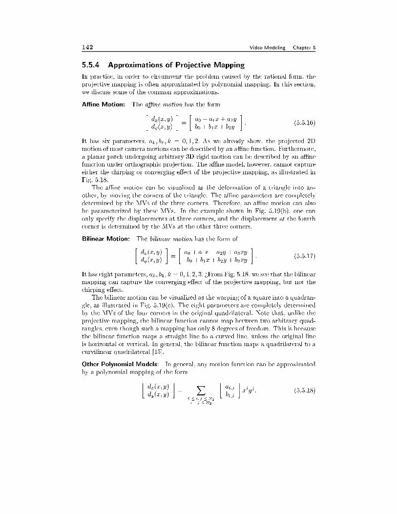
142 Video Modeling Chapter 5
5.5.4 Approximations of Projective Mapping
In practice, in order to circumvent the problem caused by the rational form, theprojective mapping is often approximated by polynomial mapping. In this section,we discuss some of the common approximations.
AÆne Motion: The aÆne motion has the form�dx(x; y)dy(x; y)
�=
�a0 + a1x+ a2y
b0 + b1x+ b2y
�: (5.5.16)
It has six parameters, ak; bk; k = 0; 1; 2: As we already show, the projected 2Dmotion of most camera motions can be described by an aÆne function. Furthermore,a planar patch undergoing arbitrary 3D rigid motion can be described by an aÆnefunction under orthographic projection. The aÆne model, however, cannot captureeither the chirping or converging e�ect of the projective mapping, as illustrated inFig. 5.18.
The aÆne motion can be visualized as the deformation of a triangle into an-other, by moving the corners of the triangle. The aÆne parameters are completelydetermined by the MVs of the three corners. Therefore, an aÆne motion can alsobe parameterized by these MVs. In the example shown in Fig. 5.19(b), one canonly specify the displacements at three corners, and the displacement at the fourthcorner is determined by the MVs at the other three corners.
Bilinear Motion: The bilinear motion has the form of�dx(x; y)dy(x; y)
�=
�a0 + a1x+ a2y + a3xy
b0 + b1x+ b2y + b3xy
�: (5.5.17)
It has eight parameters, ak; bk; k = 0; 1; 2; 3: >From Fig. 5.18, we see that the bilinearmapping can capture the converging e�ect of the projective mapping, but not thechirping e�ect.
The bilinear motion can be visualized as the warping of a square into a quadran-gle, as illustrated in Fig. 5.19(c). The eight parameters are completely determinedby the MVs of the four corners in the original quadrilateral. Note that, unlike theprojective mapping, the bilinear function cannot map between two arbitrary quad-rangles, even though such a mapping has only 8 degrees of freedom. This is becausethe bilinear function maps a straight line to a curved line, unless the original lineis horizontal or vertical. In general, the bilinear function maps a quadrilateral to acurvilinear quadrilateral [15].
Other Polynomial Models: In general, any motion function can be approximatedby a polynomial mapping of the form�
dx(x; y)dy(x; y)
�=
X0 � i; j � N1i + j � N2
�ai;jbi;j
�xiyj : (5.5.18)
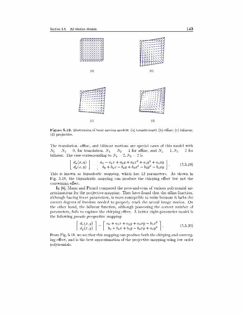
Section 5.5. 2D Motion Models 143
(a)
(c) (d)
(b)
Figure 5.19. Illustration of basic motion models: (a) translational; (b) aÆne; (c) bilinear;
(d) projective.
The translation, aÆne, and bilinear motions are special cases of this model withN1 = N2 = 0; for translation, N1 = N2 = 1 for aÆne, and N1 = 1; N2 = 2 forbilinear. The case corresponding to N1 = 2; N2 = 2 is�
dx(x; y)dy(x; y)
�=
�a0 + a1x+ a2y + a3x
2 + a4y2 + a5xy
b0 + b1x+ b2y + b3x2 + b4y
2 + b5xy
�: (5.5.19)
This is known as biquadratic mapping, which has 12 parameters. As shown inFig. 5.18, the biquadratic mapping can produce the chirping e�ect but not theconverging e�ect.
In [6], Mann and Picard compared the pros-and-cons of various polynomial ap-proximations for the projective mapping. They have found that the aÆne function,although having fewer parameters, is more susceptible to noise because it lacks thecorrect degrees of freedom needed to properly track the actual image motion. Onthe other hand, the bilinear function, although possessing the correct number ofparameters, fails to capture the chirping e�ect. A better eight-parameter model isthe following pseudo-perspective mapping:�
dx(x; y)dy(x; y)
�=
�a0 + a1x+ a2y + a3xy + b3x
2
b0 + b1x+ b2y + b3xy + a3y2
�: (5.5.20)
From Fig. 5.18, we see that this mapping can produce both the chirping and converg-ing e�ect, and is the best approximation of the projective mapping using low-orderpolynomials.
144 Video Modeling Chapter 5
5.6 Summary
In this chapter, we discussed parametric models that allow us to describe how animage sequence is generated. Depending on the application, we can use models thatmodel the real world with an appropriate amount of detail.
Camera Model
The camera model describes the projection of the 3D world on to the image planeby means of the real camera. Depending on our application, we can use cameramodels of di�erent complexity. If the objects in the 3D world are far away fromthe camera we might use a simple camera model with orthographic projection. Apinhole camera model uses a perspective projection and enables us to describe thechange of object size in an image sequence as an object changes its distance fromthe camera.
Illumination Model
In order to see an object, we need to illuminate the scene we are looking at. De-scribing illumination and the re ection of light on object surfaces requires usuallycomplex models. However, we assume the most simple illumination model for manyvideo processing applications: ambient light and di�use re ecting surfaces. Underthis model, the surface re ectance of an object does not change as the object moves.This model is sometimes referred to as constant intensity assumption. The motionestimation algorithms presented in Chaps. 6 and 7 make use of this assumptionextensively. Note that, with this model, we cannot describe shadows or glossyre ections.
Object Model
Objects are described by shape, motion and texture. The 3D shape of an object canbe described by its volume using cubes of unit length named voxels or by its surfaceusing a wireframe. We express 3D object motion by means of a 3D translationvector and a 3x3 rotation matrix that is computed from the rotation angles aroundthe three coordinate axes. Simple models can be derived by simplifying the 3D
object shape and motion models.
Scene Model
The scene model describes how the moving objects and the camera of a 3D sceneare positioned with respect to each other. In video coding, we often use a 2D scenemodel that assumes 2D objects moving parallel to the imaging plane of the camera.The slightly more complex 2.5D scene model allows us to handle object occlusion.Finally, the 3D scene model can describe the real world realistically.
Section 5.7. Problems 145
2D Motion Model
Object or camera motions in 3D lead to 2D motions. The 2D motion model dependsnot only on the 3D motion model, but also the illumination model and the cameramodel. The most important 2D motion model is the projective mapping, whichis valid over small 2D regions, when the object/camera undergoes rigid motion,the camera can be modeled by perspective projection, and the constant intensityassumptions applies. In practice, this mapping is often approximately by aÆne orbilinear mappings.
5.7 Problems
5.1 Assume a pinhole camera with focal length F = 9mm, a target of 1"� 1:33"and an image resolution of 352� 288 pels and an object point with a distanceof Z = 2 m from the camera center. Determine the projection of this pointinto the image as a function of its (X;Y ) position in 3D space. How muchdoes the point have to move in the direction of the Z-axis in order to moveits image point by 1 pel? What is the answer if we assume a camera modelwith orthographic projection?
5.2 Show that, under orthographic projection, the projected 2D motion of a planarpatch undergoing translation, rotation and scaling (because of camera zoom)can be described by an aÆne function.
5.3 Show that, under perspective projection, the projected 2D motion of a planarpatch undergoing rigid motion can be described by a projective mapping.
5.4 Show that Eq. (5.5.13) can be simpli�ed into the projective mapping givingin Eq. 5.5.14, when the imaged object has a planar surface. That is, 3Dcoordinates of points on the object satisfy aX+bY +cZ = 1 for some constantsa; b; c:
5.5 Consider a triangle whose original corner positions are at xk; k = 1; 2; 3. Sup-pose each corner is moved by dk. Determine the aÆne parameters that canrealize such a mapping.
5.6 Suppose that you are given the motion vectors dk at K > 3 points xk in animage, and that you want to use the aÆne mapping to approximate the overallmotion. How do you determine the aÆne parameters?
Hint: use a least squares �tting method.
5.7 Repeat 5.5 for the bilinear mapping between two quadrangles. Assume thatdisplacements at K=4 points are available.
5.8 Repeat 5.6 for the bilinear mapping, assuming K > 4.
146 Video Modeling Chapter 5
5.9 Repeat 5.5 for the projective mapping between two quadrangles. Assume thatdisplacements at K=4 points are available.
Hint: you can still set-up a linear equation in terms of the parameters ak; bk; ck. The
constants in the left side of the equation will contain both xk and x0
k= xk + dk.
5.10 Repeat 5.6 for the projective mapping, assuming K > 4.
5.8 Bibliography
[1] G. Bozdagi, A. M. Tekalp, and L. Onural. 3-D motion estimation and wireframeadaptation including photometric e�ects for model-based coding of facial imagesequences. IEEE Trans. Circuits Syst. for Video Technology, 4(3):246{256, June1994.
[2] O. Faugeras. Three-Dimensional Computer Vision - A Geometric Viewpoint.The MIT Press, 1993.
[3] J. Foley, A. van Dam, S. K. Feiner, J. F. Hughes, and R. L. Phillips. Introductionto Computer Graphics. Addison-Wesley Publishing Company, 1994.
[4] M. Gilge. Motion estimation by scene adaptive block matching (SABM) andillumination correction. In SPIE, Santa Clara, February 1990. SPIE.
[5] M. H�otter and R. Thoma. Image segmentation based on object oriented mappingparameter estimation. Signal Processing, 15(3):315{334, October 1988.
[6] S. Mann and R. W. Picard. Video orbits of the projective group: A simpleapproach to featureless estimation of parameters. IEEE Trans. Image Process.,6:1281{1295, Sept. 1997.
[7] H. G. Musmann, M. Hotter, and J. Ostermann. Object oriented analysis-synthesis coding of moving images. Signal Processing: Image Commun., 1:119{138,Oct. 1989.
[8] W. Niem. Robust and fast modelling of 3D natural objects from multiple views.In SPIE Image and Video Processing II, volume 2182, pages 388{397, 1994. cahvcamera model.
[9] J. Ostermann. Segmentation of image areas changed due to object motionconsidering shadows. In Y. Wang et al., editors, Multimedia Communications and
Video Coding. Plenum Press, 1996.
[10] M. Pollefeys, R. Koch, and L. Van Gool. Self calibration and metric reconstruc-tion in spite of varying and unknown internal camera parameters. In Proceedings
ICCV 98, pages 90{96, 1998.
[11] D. F. Rogers. Procedural elements for computer graphics. McGraw-Hill, Sin-gapore, 1985.
Section 5.8. Bibliography 147
[12] J. Stauder. An illumination estimation method for 3D-object-based analysis-synthesis coding. In COST 211 European Workshop, pages 4.51{4.5.6, Universityof Hannover, Germany, December 1993.
[13] J. Stauder. Estimation of point light source parameters for object-based coding.Signal processing: Image Communication, 46(7):355{379, 1995.
[14] J. Stauder, R. Mech, and J. Ostermann. Detection of moving cast shadows forobject segmentation. IEEE Transactions on Multimedia, 1(1):65{76, March 1999.
[15] G. Wolberg. Digital Image Warping. IEEE Computer Society Press, LosAlamitos, CA, 1990.
[16] Y. Yakimovsky and R. Cunningham. A system for extracting three-dimensionalmeasurements from a stereo pair of TV cameras. Computer Graphics and Image
Processing, 7(2):195{210, April 1978.
Chapter 6
TWO DIMENSIONAL
MOTION ESTIMATION
Motion estimation is an important part of any video processing system. In this
chapter, we are only concerned with the estimation of 2D motion. In Chapter 7,
we will discuss estimation of actual 3D motion. As will be seen, 2D motion estima-
tion is often a preprocessing step required for 3D structure and motion estimation.
Also, 2D motion estimation itself has a wide range of applications, including video
compression, video sampling rate conversion, video �ltering, etc. Depending on
the intended applications for the resulting 2D motion vectors, motion estimation
methods could be very di�erent. For example, for computer vision applications,
where the 2D motion vectors are to be used to deduce 3D structure and motion
parameters, a sparse set of 2D motion vectors at critical feature points may be
suÆcient. The motion vectors must be physically correct for them to be useful. On
the other hand, for video compression applications, the estimated motion vectors
are used to produce a motion-compensated prediction of a frame to be coded from
a previously coded reference frame. The ultimate goal is to minimize the total bits
used for coding the motion vectors and the prediction errors. There is a trade-o�
that one can play between the accuracy of the estimated motion, and the number
of bits used to specify the motion. Sometimes, even when the estimated motion
is not an accurate representation of the true physical motion, it can still lead to
good temporal prediction and in that regard is considered a good estimate. In this
chapter, we focus on the type of motion estimation algorithms targeted for motion
compensated processing (prediction, �ltering, interpolation, etc.). For additional
readings on this topic, the reader is referred to the review papers by Musmann et
al. [28] and by Stiller and Konrad [38]. For a good treatment of motion estimation
methods for computer vision applications, please see the article by Aggarwal and
Nandhahumar [1].
All the motion estimation algorithms are based on temporal changes in image
intensities (more generally color). In fact, the observed 2D motions based on inten-
sity changes may not be the same as the actual 2D motions. To be more precise,
the velocity of observed or apparent 2D motion vectors are referred to as optical
148
Section 6.1. Optical Flow 149
ow. Optical ow can be caused not only by object motions, but also camera
movements or illumination condition changes. In this chapter, we start by de�ning
optical ow. We then derive the optical ow equation, which imposes a constraint
between image gradients and ow vectors. This is a fundamental equality that many
motion estimation algorithms are based on. Next we present the general method-
ologies for 2D motion estimation. As will be seen, motion estimation problem is
usually converted to an optimization problem and involves three key components:
parameterization of the motion �eld, formulation of the optimization criterion, and
�nally searching of the optimal parameters. Finally, we present motion estimation
algorithms developed based on di�erent parameterizations of the motion �eld and
di�erent estimation criteria. Unless speci�ed otherwise, the word \motion" refers
to 2D motion, in this chapter.
6.1 Optical Flow
6.1.1 2D Motion vs. Optical Flow
The human eye perceives motion by identifying corresponding points at di�erent
times. The correspondence is usually determined by assuming that the color or
brightness of a point does not change after the motion. It is interesting to note
that the observed 2D motion can be di�erent from the actual projected 2D motion
under certain circumstances. Figure 6.1 illustrates two special cases. In the �rst
example, a sphere with a uniform at surface is rotating under a constant ambient
light. Because every point on the sphere re ects the same color, the eye cannot
observe any change in the color pattern of the imaged sphere and thus considers
the sphere as being stationary. In the second example, the sphere is stationary,
but is illuminated by a point light source that is rotating around the sphere. The
motion of the light source causes the movement of the re ecting light spot on the
sphere, which in turn can make the eye believe the sphere is rotating. The observed
or apparent 2D motion is referred to as optical ow in computer vision literature.
The above examples reveal that the optical ow may not be the same as the true
2D motion. When only image color information is available, the best one can hope
to estimate accurately is the optical ow. However, in the remaining part of this
chapter, we will use the term 2D motion or simply motion to describe optical ow.
The readers should bear in mind that sometimes it may be di�erent from the true
2D motion.
6.1.2 Optical Flow Equation and Ambiguity in Motion Estimation
Consider a video sequence whose luminance variation is represented by (x; y; t):1
Suppose an imaged point (x; y) at time t is moved to (x+ dx; y+ dy) at time t+ dt.
Under the constant intensity assumption introduced in Sec. 5.2.3 (Eq. (5.2.11)), the
1In this book, we only consider motion estimation based on the luminance intensity information,
although the same methodology can be applied to the full color information.
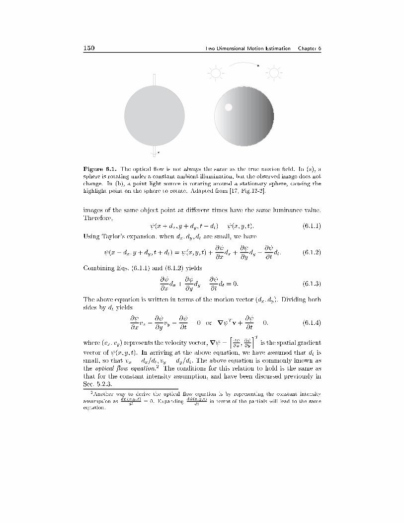
150 Two Dimensional Motion Estimation Chapter 6
Figure 6.1. The optical ow is not always the same as the true motion �eld. In (a), a
sphere is rotating under a constant ambient illumination, but the observed image does not
change. In (b), a point light source is rotating around a stationary sphere, causing the
highlight point on the sphere to rotate. Adapted from [17, Fig.12-2].
images of the same object point at di�erent times have the same luminance value.
Therefore,
(x+ dx; y + dy ; t+ dt) = (x; y; t): (6.1.1)
Using Taylor's expansion, when dx; dy; dt are small, we have
(x + dx; y + dy; t+ dt) = (x; y; t) +@
@xdx +
@
@ydy +
@
@tdt: (6.1.2)
Combining Eqs. (6.1.1) and (6.1.2) yields
@
@xdx +
@
@ydy +
@
@tdt = 0: (6.1.3)
The above equation is written in terms of the motion vector (dx; dy). Dividing both
sides by dt yields
@
@xvx +
@
@yvy +
@
@t= 0 or r Tv +
@
@t= 0: (6.1.4)
where (vx; vy) represents the velocity vector,r =h@
@x; @ @y
iTis the spatial gradient
vector of (x; y; t). In arriving at the above equation, we have assumed that dt is
small, so that vx = dx=dt; vy = dy=dt: The above equation is commonly known as
the optical ow equation.2 The conditions for this relation to hold is the same as
that for the constant intensity assumption, and have been discussed previously in
Sec. 5.2.3.2Another way to derive the optical ow equation is by representing the constant intensity
assumption asd (x;y;t)
dt= 0. Expanding
d (x;y;t)
dtin terms of the partials will lead to the same
equation.
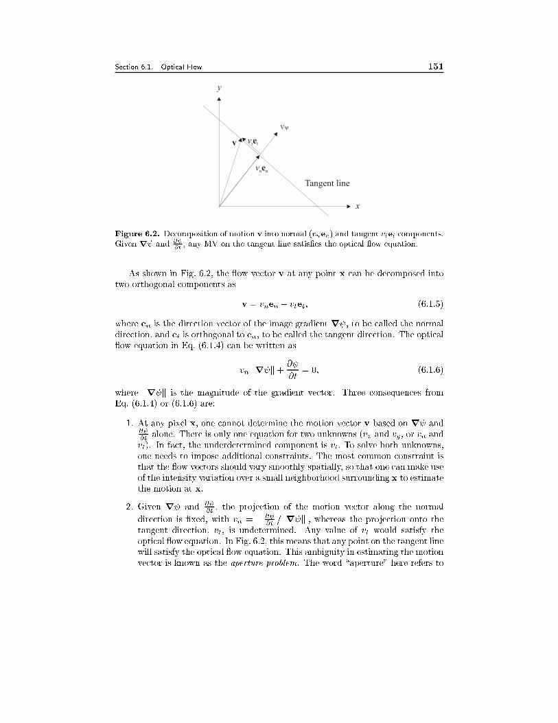
Section 6.1. Optical Flow 151
v vt te
vn ne
x
y
Tangent line
��
Figure 6.2. Decomposition of motion v into normal (vnen) and tangent vtet components.
Given r and @
@t; any MV on the tangent line satis�es the optical ow equation.
As shown in Fig. 6.2, the ow vector v at any point x can be decomposed into
two orthogonal components as
v = vnen + vtet; (6.1.5)
where en is the direction vector of the image gradient r , to be called the normal
direction, and et is orthogonal to en, to be called the tangent direction. The optical
ow equation in Eq. (6.1.4) can be written as
vn kr k+@
@t= 0; (6.1.6)
where kr k is the magnitude of the gradient vector. Three consequences from
Eq. (6.1.4) or (6.1.6) are:
1. At any pixel x, one cannot determine the motion vector v based on r and@
@talone. There is only one equation for two unknowns (vx and vy, or vn and
vt). In fact, the underdetermined component is vt: To solve both unknowns,
one needs to impose additional constraints. The most common constraint is
that the ow vectors should vary smoothly spatially, so that one can make use
of the intensity variation over a small neighborhood surrounding x to estimate
the motion at x.
2. Given r and @
@t; the projection of the motion vector along the normal
direction is �xed, with vn = �@
@t/kr k ; whereas the projection onto the
tangent direction, vt, is undetermined. Any value of vt would satisfy the
optical ow equation. In Fig. 6.2, this means that any point on the tangent line
will satisfy the optical ow equation. This ambiguity in estimating the motion
vector is known as the aperture problem. The word \aperture" here refers to
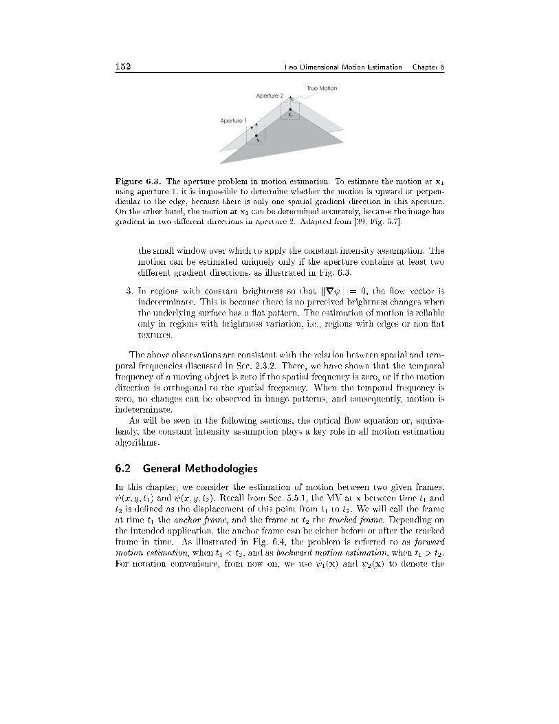
152 Two Dimensional Motion Estimation Chapter 6
Aperture 1
Aperture 2
True Motion
x1
x2
Figure 6.3. The aperture problem in motion estimation: To estimate the motion at x1using aperture 1, it is impossible to determine whether the motion is upward or perpen-
dicular to the edge, because there is only one spatial gradient direction in this aperture.
On the other hand, the motion at x2 can be determined accurately, because the image has
gradient in two di�erent directions in aperture 2. Adapted from [39, Fig. 5.7].
the small window over which to apply the constant intensity assumption. The
motion can be estimated uniquely only if the aperture contains at least two
di�erent gradient directions, as illustrated in Fig. 6.3.
3. In regions with constant brightness so that kr k = 0; the ow vector is
indeterminate. This is because there is no perceived brightness changes when
the underlying surface has a at pattern. The estimation of motion is reliable
only in regions with brightness variation, i.e., regions with edges or non- at
textures.
The above observations are consistent with the relation between spatial and tem-
poral frequencies discussed in Sec. 2.3.2. There, we have shown that the temporal
frequency of a moving object is zero if the spatial frequency is zero, or if the motion
direction is orthogonal to the spatial frequency. When the temporal frequency is
zero, no changes can be observed in image patterns, and consequently, motion is
indeterminate.
As will be seen in the following sections, the optical ow equation or, equiva-
lently, the constant intensity assumption plays a key role in all motion estimation
algorithms.
6.2 General Methodologies
In this chapter, we consider the estimation of motion between two given frames,
(x; y; t1) and (x; y; t2). Recall from Sec. 5.5.1, the MV at x between time t1 and
t2 is de�ned as the displacement of this point from t1 to t2. We will call the frame
at time t1 the anchor frame, and the frame at t2 the tracked frame. Depending on
the intended application, the anchor frame can be either before or after the tracked
frame in time. As illustrated in Fig. 6.4, the problem is referred to as forward
motion estimation, when t1 < t2, and as backward motion estimation, when t1 > t2.
For notation convenience, from now on, we use 1(x) and 2(x) to denote the
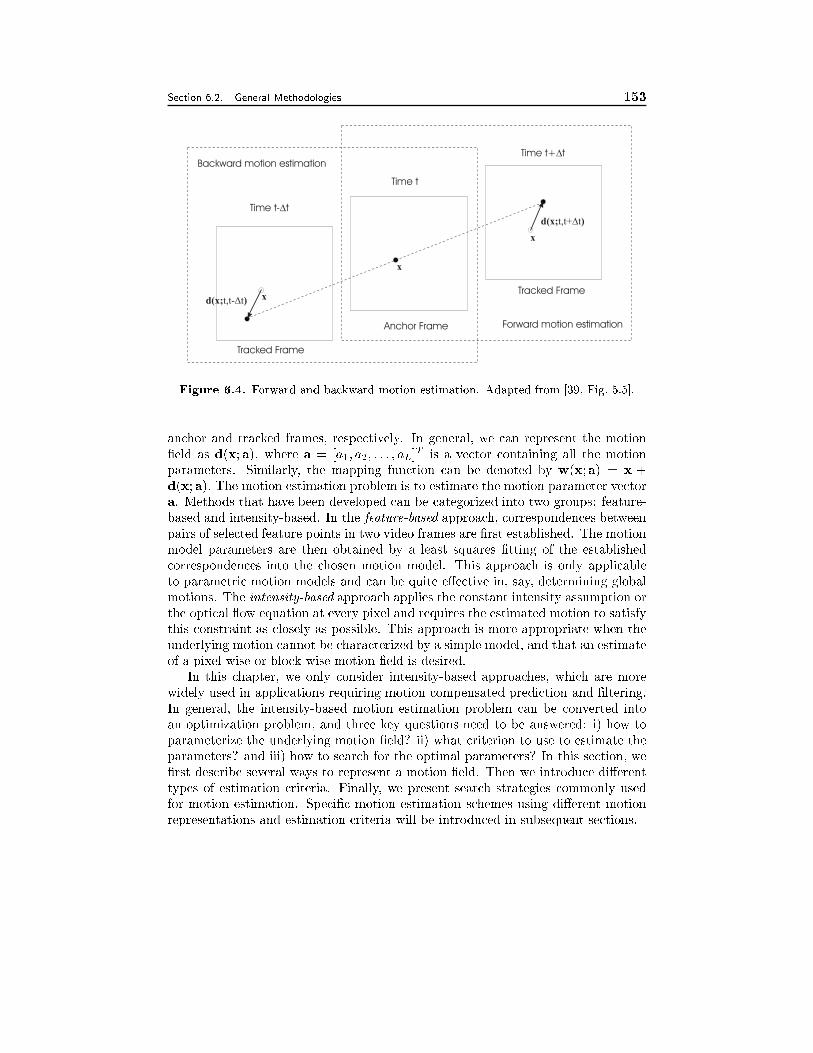
Section 6.2. General Methodologies 153
x
x
d(x; )t,t+ t�
d(x; )t,t- t�
x
Time t
Time t+ t�
Time t- t�
Forward motion estimation
Backward motion estimation
Anchor Frame
Tracked Frame
Tracked Frame
Figure 6.4. Forward and backward motion estimation. Adapted from [39, Fig. 5.5].
anchor and tracked frames, respectively. In general, we can represent the motion
�eld as d(x; a), where a = [a1; a2; : : : ; aL]T is a vector containing all the motion
parameters. Similarly, the mapping function can be denoted by w(x; a) = x +
d(x; a): The motion estimation problem is to estimate the motion parameter vector
a. Methods that have been developed can be categorized into two groups: feature-
based and intensity-based. In the feature-based approach, correspondences between
pairs of selected feature points in two video frames are �rst established. The motion
model parameters are then obtained by a least squares �tting of the established
correspondences into the chosen motion model. This approach is only applicable
to parametric motion models and can be quite e�ective in, say, determining global
motions. The intensity-based approach applies the constant intensity assumption or
the optical ow equation at every pixel and requires the estimated motion to satisfy
this constraint as closely as possible. This approach is more appropriate when the
underlying motion cannot be characterized by a simple model, and that an estimate
of a pixel-wise or block-wise motion �eld is desired.
In this chapter, we only consider intensity-based approaches, which are more
widely used in applications requiring motion compensated prediction and �ltering.
In general, the intensity-based motion estimation problem can be converted into
an optimization problem, and three key questions need to be answered: i) how to
parameterize the underlying motion �eld? ii) what criterion to use to estimate the
parameters? and iii) how to search for the optimal parameters? In this section, we
�rst describe several ways to represent a motion �eld. Then we introduce di�erent
types of estimation criteria. Finally, we present search strategies commonly used
for motion estimation. Speci�c motion estimation schemes using di�erent motion
representations and estimation criteria will be introduced in subsequent sections.
154 Two Dimensional Motion Estimation Chapter 6
6.2.1 Motion Representation
A key problem in motion estimation is how to parameterize the motion �eld. As
shown in Sec. 5.5, the 2D motion �eld resulting from a camera or object motion
can usually be described by a few parameters. However, usually, there are multiple
objects in the imaged scene that move di�erently. Therefore, a global parameterized
model is usually not adequate. The most direct and unconstrained approach is to
specify the motion vector at every pixel. This is the so-called pixel-based representa-
tion. Such a representation is universally applicable, but it requires the estimation
of a large number of unknowns (twice the number of pixels!) and the solution can
often be physically incorrect unless a proper physical constraint is imposed during
the estimation step. On the other hand, if only the camera is moving or the imaged
scene contains a single moving object with a planar surface, one could use a global
motion representation to characterize the entire motion �eld. In general, for scenes
containing multiple moving objects, it is more appropriate to divide an image frame
into multiple regions so that the motion within each region can be characterized well
by a parameterized model. This is known as region-based motion representation,3
which consists of a region segmentation map and several sets of motion parameters,
one for each region. The diÆculty with such an approach is that one does not
know in advance which pixels have similar motions. Therefore, segmentation and
estimation have to be accomplished iteratively, which requires intensive amount of
computations that may not be feasible in practice.
One way to reduce the complexity associated with region-based motion repre-
sentation is by using a �xed partition of the image domain into many small blocks.
As long as each block is small enough, the motion variation within each block can
be characterized well by a simple model and the motion parameters for each block
can be estimated independently. This brings us to the popular block-based repre-
sentation. The simplest version models the motion in each block by a constant
translation, so that the estimation problem becomes that of �nding one MV for
each block. This method provides a good compromise between accuracy and com-
plexity, and has found great success in practical video coding systems. One main
problem with the block-based approach is that it does not impose any constraint
on the motion transition between adjacent blocks. The resulting motion is often
discontinuous across block boundaries, even when the true motion �eld is changing
smoothly from block to block. One approach to overcome this problem is by using
a mesh-based representation, by which the underlying image frame is partitioned
into non-overlapping polygonal elements. The motion �eld over the entire frame
is described by the MVs at the nodes (corners of polygonal elements) only, and
the MVs at the interior points of an element are interpolated from the nodal MVs.
This representation induces a motion �eld that is continuous everywhere. It is more
appropriate than the block-based representation over interior regions of an object,
3This is sometimes called object-based motion representation [27]. Here we use the word \region-
based" to acknowledge the fact that we are only considering 2D motions, and that a region with
a coherent 2D motion may not always correspond to a physical object.
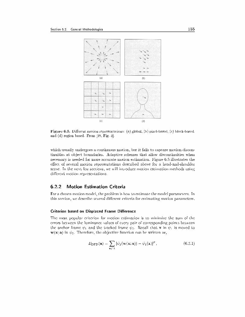
Section 6.2. General Methodologies 155
Figure 6.5. Di�erent motion representations: (a) global, (b) pixel-based, (c) block-based,
and (d) region-based. From [38, Fig. 3].
which usually undergoes a continuous motion, but it fails to capture motion discon-
tinuities at object boundaries. Adaptive schemes that allow discontinuities when
necessary is needed for more accurate motion estimation. Figure 6.5 illustrates the
e�ect of several motion representations described above for a head-and-shoulder
scene. In the next few sections, we will introduce motion estimation methods using
di�erent motion representations.
6.2.2 Motion Estimation Criteria
For a chosen motion model, the problem is how to estimate the model parameters. In
this section, we describe several di�erent criteria for estimating motion parameters.
Criterion based on Displaced Frame Di�erence
The most popular criterion for motion estimation is to minimize the sum of the
errors between the luminance values of every pair of corresponding points between
the anchor frame 1 and the tracked frame 2. Recall that x in 1 is moved to
w(x; a) in 2. Therefore, the objective function can be written as,
EDFD(a) =Xx2�
j 2(w(x; a)) � 1(x)jp; (6.2.1)
156 Two Dimensional Motion Estimation Chapter 6
where � is the domain of all pixels in 1, and p is a positive number. When p = 1,
the above error is called mean absolute di�erence (MAD), and when p = 2, the
mean squared error (MSE). The error image, e(x; a) = 2(w(x; a)) � 1(x), is
usually called displaced frame di�erence (DFD) image, and the above measure the
DFD error.
The necessary condition for minimizing EDFD is that its gradient vanishes. In
the case of p = 2, this gradient is
@EDFD
@a= 2
Xx2�
( 2(w(x; a)) � 1(x))@d(x)
@ar 2(w(x; a)) (6.2.2)
where
@d
@a=
"@dx
@a1
@dx
@a2� � � @dx
@aL@dy
@a1
@dy
@a2� � �
@dy
@aL
#T:
Criterion based on Optical Flow Equation
Instead of minimizing the DFD error, another approach is to solve the system
of equations established based on the optical ow constraint given in Eq. (6.1.3).
Let 1(x; y) = (x; y; t); 2(x; y) = (x; y; t + dt): If dt is small, we can assume@
@tdt = 2(x) � 1(x): Then, Eq. (6.1.3) can be written as
@ 1
@xdx +
@ 1
@ydy + ( 2 � 1) = 0 or r T1 d+ ( 2 � 1) = 0: (6.2.3)
This discrete version of the optical ow equation is more often used for motion
estimation in digital videos. Solving the above equations for all x can be turned
into a minimization problem with the following objective function:
E ow(a) =Xx2�
��r 1(x)Td(x; a) + 2(x)� 1(x)��p : (6.2.4)
The gradient of E ow is, when p = 2;
@E ow
@a= 2
Xx2�
�r 1(x)
Td(x; a) + 2(x)� 1(x)� @d(x)
@ar 1(x): (6.2.5)
If the motion �eld is constant over a small region �0, i.e., d(x; a) = d0;x 2 �0,
then Eq. (6.2.5) becomes
@E ow
@d0=Xx2�0
�r 1(x)
Td0 + 2(x) � 1(x)�r 1(x): (6.2.6)
Setting the above gradient to zero yields the least squares solution for d0:
d0 =
Xx2�0
r 1(x)r 1(x)T
!�1 Xx2�0
( 1(x) � 2(x))r 1(x)
!: (6.2.7)

Section 6.2. General Methodologies 157
When the motion is not a constant, but can be related to the model parameters
linearly, one can still derive a similar least-squares solution. See Prob. 6.6 in the
Problem section.
An advantage of the above method is that the minimizing function is a quadratic
function of the MVs, when p = 2. If the motion parameters are linearly related
to the MVs, then the function has a unique minimum and can be solved easily.
This is not true with the DFD error given in Eq. (6.2.1). However, the optical
ow equation is valid only when the motion is small, or when an initial motion
estimate ~d(x) that is close to the true motion can be found and one can pre-update
2(x) to 2(x+ ~d(x)) When this is not the case, it is better to use the DFD error
criterion, and �nd the minimal solution using the gradient descent or exhaustive
search method.
Regularization
Minimizing the DFD error or solving the optical ow equation does not always give
physically meaningful motion estimate. This is partially because the constant inten-
sity assumption is not always correct. The imaged intensity of the same object point
may vary after an object motion because of the various re ectance and shadowing
e�ects. Secondly, in a region with at texture, many di�erent motion estimates can
satisfy the constant intensity assumption or the optical ow equation. Finally, if the
motion parameters are the MVs at every pixel, the optical ow equation does not
constrain the motion vector completely. These factors make the problem of motion
estimation a ill-posed problem.
To obtain a physically meaningful solution, one needs to impose additional con-
straints to regularize the problem. One common regularization approach is to add
a penalty term to the error function in (6.2.1) or (6.2.4), which should enforce the
resulting motion estimate to bear the characteristics of common motion �elds. One
well-known property of a typical motion �eld is that it usually varies smoothly from
pixel to pixel, except at object boundaries. To enforce the smoothness, one can use
a penalty term that measures the di�erences between the MVs of adjacent pixels,
i.e.,
Es(a) =Xx2�
Xy2Nx
kd(x; a) � d(y; a)k2; (6.2.8)
where k � k represents the 2-norm, Nx represents the set of pixels adjacent to x.
Either the 4-connectivity or 8-connectivity neighborhood can be used.
The overall minimization criterion can be written as
E = EDFD + wsEs: (6.2.9)
The weighting coeÆcient ws should be chosen based on the importance of motion
smoothness relative to the prediction error. To avoid over-blurring, one should re-
duce the weighting at object boundaries. This, however, requires accurate detection
of object boundaries, which is not a trivial task.
158 Two Dimensional Motion Estimation Chapter 6
Bayesian Criterion
The Bayesian estimator is based on a probablistic formulation of the motion esti-
mation problem, pioneered by Konrad and Dubois [22, 38]. Under this formulation,
given an anchor frame 1, the image function at the tracked frame 2 is considered
a realization of a random �eld , and the motion �eld d is a realization of another
random �eld D . The a posterior probability distribution of the motion �eld D
given a realization of and 1 can be written, using the Bayes rule
P (D = dj = 2; 1) =P ( = 2jD = d; 1)P (D = d; 1)
P ( = 2; 1): (6.2.10)
In the above notation, the semicolon indicates that subsequent variables are de-
terministic parameters. An estimator based on the Bayesian criterion attempts to
maximize the a posterior probability. But for given 1 and 2, maximizing the
above probability is equivalent to maximizing the numerator only. Therefore, the
maximum a posterior (MAP) estimate of d is
dMAP = argmaxd fP ( = 2jD = d; 1)P (D = d; 1)g : (6.2.11)
The �rst probability denotes the likelihood of an image frame given the motion
�eld and the anchor frame. Let E represent the random �eld corresponding to the
DFD image e(x) = 2(x+ d)� 1(x) for given d and 1, then
P ( = 2jD = d; 1) = P (E = e);
and the above equation becomes
dMAP = argmaxd fP (E = e)P (D = d; 1)g
= argmind f� logP (E = e)� logP (D = d; 1)g : (6.2.12)
From the source coding theory (Sec. 8.3.1), the minimum coding length for a
source X is its entropy, � logP (X = x). We see that the MAP estimate is
equivalent to minimizing the sum of the coding length for the DFD image e and
that for the motion �eld d. As will be shown in Sec. 9.3.1, this is precisely what
a video coder using motion-compensated prediction needs to code. Therefore, the
MAP estimate for d is equivalent to a minimum description length (MDL) estimate
[34]. Because the purpose of motion estimation in video coding is to minimize the
bit rate, the MAP criterion is a better choice than minimizing the prediction error.
The most common model for the DFD image is a zero-mean independently
identically distributed (i.i.d.) Gaussian �eld, with distribution
P (E = e) = (2��2)�j�j=2 exp�P
x2� e2(x)
2�2; (6.2.13)
where j�j denotes the size of � (i.e., the number of pixels in �). With this model,
minimizing the �rst term in Eq. (6.2.12) is equivalent to minimizing the previously
de�ned DFD error (when p = 2).
Section 6.2. General Methodologies 159
For the motion �eld D , a common model is a Gibbs/Markov random �eld [11].
Such a model is de�ned by a neighborhood structure called clique. Let C represent
the set of cliques, the model assumes
P (D = d) =1
Zexp(�
Xc2C
Vc(d)); (6.2.14)
where Z is a normalization factor. The function Vc(d) is called the potential func-
tion, which is usually de�ned to measure the di�erence between pixels in the same
clique:
Vc(d) =X
(x;y)2c
jd(x)� d(y)j2: (6.2.15)
Under this model, minimizing the second term in Eq. (6.2.12) is equivalent to min-
imizing the smoothing function in Eq. (6.2.8). Therefore, the MAP estimate is
equivalent to the DFD-based estimator with an appropriate smoothness constraint.
6.2.3 Minimization Methods
The error functions presented in Sec. 6.2.2 can be minimized using various opti-
mization methods. Here we only consider exhaustive search and gradient-based
search methods. Usually, for the exhaustive search, the MAD is used for reasons of
computational simplicity, whereas for the gradient-based search, the MSE is used
for its mathematical tractability.
Obviously, the advantage of the exhaustive search method is that it guarantees
reaching the global minimum. However, such search is feasible only if the number of
unknown parameters is small, and each parameter takes only a �nite set of discrete
values. To reduce the search time, various fast algorithms can be developed, which
achieve sub-optimal solutions.
The most common gradient descent methods include the steepest gradient de-
scent and the Newton-Ralphson method. A brief review of these methods is provided
in Appendix B. A gradient-based method can handle unknown parameters in a high
dimensional continuous space. However, it can only guarantee the convergence to
a local minimum. The error functions introduced in the previous section in general
are not convex and can have many local minima that are far from the global mini-
mum. Therefore, it is important to obtain a good initial solution through the use of
a prior knowledge, or by adding a penalty term to make the error function convex.
With the gradient-based method, one must calculate the spatio-temporal gradi-
ents of the underlying signal. Appendix A reviews methods for computing �rst and
second order gradients from digital sampled images. Note that the methods used
for calculating the gradient functions can have profound impact on the accuracy
and robustness of the associated motion estimation methods, as have been shown
by Barron et al. [4]. Using a Gaussian pre-�lter followed by a central di�erence
generally leads to signi�cantly better results than the simple two point di�erence
approximation.
160 Two Dimensional Motion Estimation Chapter 6
One important search strategy is to use a multi-resolution representation of the
motion �eld and conduct the search in a hierarchical manner. The basic idea is to
�rst search the motion parameters in a coarse resolution, propagate this solution
into a �ner resolution, and then re�ne the solution in the �ner resolution. It can
combat both the slowness of exhaustive search methods and the non-optimality
of gradient-based methods. We will present the multi-resolution method in more
detail in Sec. 6.9.
6.3 Pixel-Based Motion Estimation
In pixel-based motion estimation, one tries to estimate a motion vector for ev-
ery pixel. Obviously, this problem is ill-de�ned. If one uses the constant inten-
sity assumption, for every pixel in the anchor frame, there are many pixels in the
tracked frame that have exactly the same image intensity. If one uses the optical
ow equation instead, the problem is again indeterminate, because there is only
one equation for two unknowns. To circumvent this problem, there are in general
four approaches. First, one can use the regularization technique to enforce some
smoothness constraints on the motion �eld, so that the motion vector of a new pixel
is constrained by those found for surrounding pixels. Second, one can assume the
motion vectors in a neighborhood surrounding each pixel are the same, and apply
the constant intensity assumption or the optical ow equation over the entire neigh-
borhood. The third approach is to make use of additional invariance constraints.
In addition to intensity invariance, which leads to the optical ow equation, one
can assume that the intensity gradient is invariant under motion, as proposed in
[29, 26, 15]. Finally, one can also make use of the relation between the phase func-
tions of the frame before and after motion [9]. In [4], Barron, et al. evaluated
various methods for optical ow computation, by testing these algorithms on both
synthetic and real world imageries. In this section, we will describe the �rst two
approaches only. We will also introduce the pel-recursive type of algorithms which
are developed for video compression applications.
6.3.1 Regularization Using Motion Smoothness Constraint
Horn and Schunck [16] proposed to estimate the motion vectors by minimizing the
following objective function, which is a combination of the ow-based criterion and
a motion smoothness criterion:
E (v(x)) =Xx2�
�@
@xvx +
@
@yvy +
@
@t
�2
+ ws�krvxk
2 + krvyk2�: (6.3.1)
In their original algorithm, the spatial gradient of vx and vy are approximated by
rvx = [vx(x; y) � vx(x � 1; y); vx(x; y) � vx(x; y � 1)]T ;rvy = [vy(x; y) � vy(x �1; y); vy(x; y) � vy(x; y � 1)]T : The minimization of the above error function is ac-
complished by a gradient-based method known as Gauss-Siedel method.
Section 6.3. Pixel-Based Motion Estimation 161
Nagle and Enkelmann conducted a comprehensive evaluation of the e�ect of
smoothness constraints on motion estimation [30]. In order to avoid over-smoothing
of the motion �eld, Nagel suggested an oriented-smoothness constraint in which
smoothness is imposed along the object boundaries, but not across the boundaries
[29]. This has resulted in signi�cant improvement in motion estimation accuracy
[4].
6.3.2 Using a Multipoint Neighborhood
In this approach, when estimating the motion vector at a pixel xn, we assume that
the motion vectors of all the pixels in a neighborhood B(xn) surrounding it are thesame, being dn. To determine dn, one can either minimize the prediction error over
B(xn), or solve the optical ow equation using a least squares method. Here we
present the �rst approach. To estimate the motion vector dn for xn, we minimize
the DFD error over B(xn):
En(dn) =1
2
Xx2B(xn)
w(x) ( 2(x+ dn)� 1(x))2; (6.3.2)
where w(x) are the weights assigned to pixel x. Usually, the weight decreases as
the distance from x to xn increases.
The gradient with respect to dn is
gn =@En
@dn=
Xx2B(xn)
w(x)e(x;dn)@ 2
@x
����x+dn
; (6.3.3)
where e(x;dn) = 2(x+dn)� 1(x) is the DFD at x with the estimate dn. Let dln
represent the estimate at the l-th iteration, the �rst order gradient descent method
would yield the following update algorithm
dl+1n
= dln� �gn(d
l
n): (6.3.4)
From Eq. (6.3.3), the update at each iteration depends on the sum of the image
gradients at various pixels scaled by the weighted DFD values at those pixels.
One can also derive an iterative algorithm using the Newton-Ralphson method.
From Eq. (6.3.3), the Hessian matrix is
Hn =@2En
@d2n
=X
x2B(xn)
w(x)@ 2
@x
@ 2
@x
T
�����x+dn
+ w(x)e(x;dn)@2 2
@x2
����x+dn
�X
x2B(xn)
w(x)@ 2
@x
@ 2
@x
T
�����x+dn
:
The Newton-Ralphson update algorithm is then (See Appendix B):
dl+1n
= dln� �H(dl
n)�1gn(d
l
n): (6.3.5)
162 Two Dimensional Motion Estimation Chapter 6
This algorithm converges faster than the �rst order gradient descent method, but
it requires more computation in each iteration.
Instead of using gradient-based update algorithms, one can also use exhaustive
search to �nd the dn that yields the minimal error within a de�ned search range.
This will lead to the exhaustive block matching algorithm (EBMA) to be presented
in Sec. 6.4.1. The di�erence from the EBMA is that the neighborhood used here is
a sliding window and a MV is determined for each pixel by minimizing the error in
its neighborhood. The neighborhood in general does not have to be a rectangular
block.
6.3.3 Pel-Recursive Methods
In a video coder using motion compensated prediction, one needs to specify both
the MVs and the DFD image. With a pixel-based motion representation, one would
need to specify a MV for each pixel, which is very costly. In pel-recursive motion
estimation methods, which are developed for video coding applications, the MVs
are obtained recursively. Speci�cally, the MV at a current pixel is updated from
those of its neighboring pixels that are coded before. The decoder can derive the
same MV following the same update rule, so that the MVs do not need to be coded.
A variety of such algorithms have been developed, where the update rules all follow
some types of gradient-descent methods [31].
Although pel-recursive methods are very simple, their motion estimation ac-
curacy is quite poor. As a result, the prediction error is still large and requires
a signi�cant number of bits to code. These algorithms have been used in earlier
generations of video codecs because of their simplicity. Today's codecs use more
sophisticated motion estimation algorithms, which can provide a better trade-o�
between the bits used for specifying MVs and the DFD image. The most popular
one is the block matching algorithm to be discussed in the next section.
6.4 Block Matching Algorithm
As already seen, a problem with pixel-based motion estimation is that one must
impose some smoothness constraints to regularize the problem. One way of imposing
smoothness constraints on the estimated motion �eld is to divide the image domain
into non-overlapping small regions, called blocks, and assume that the motion within
each block can be characterized by a simple parametric model, e.g., constant, aÆne,
or bilinear. If the block is suÆciently small, then this model can be quite accurate.
In this section, we describe motion estimation algorithms developed using the block-
based motion representation. We will use Bm to represent the m-th image block,
M the number of blocks, and M = f1; 2; : : : ;Mg. The partition into blocks should
satisfy
[m2M
Bm = �; and Bm\Bn = ;;m 6= n:

Section 6.4. Block Matching Algorithm 163
Theoretically, a block can have any polygonal shape. But in practice, the square
shape is used almost exclusively. The triangular shape has also been used, which is
more appropriate when the motion in each block is described by an aÆne model.
In the simplest case, the motion in each block is assumed to be constant, i.e.,
the entire block undergoes a translation. This is called the block-wise translational
model. In this section, we consider this simple case only, where the motion esti-
mation problem is to �nd a single MV for each block. This type of algorithm is
collectively referred as block matching algorithm (BMA). In the next section, we
will consider the more general case where the motion in each block is characterized
by a more complex model.
6.4.1 The Exhaustive Search Block Matching Algorithm (EBMA)
Given an image block in the anchor frame Bm, the motion estimation problem at
hand is to determine a matching block B0m
in the tracked frame so that the error
between these two blocks is minimized. The displacement vector dm between the
spatial positions of these two blocks (the center or a selected corner) is the MV of
this block. Under the block-wise translational model, w(x; a) = x + dm;x 2 Bm,the error in Eq. (6.2.1) can be written as:
E(dm;8m 2 M) =Xm2M
Xx2Bm
j 2(x + dm)� 1(x)jp: (6.4.1)
Because the estimated MV for a block only a�ects the prediction error in this block,
one can estimate the MV for each block individually, by minimizing the prediction
error accumulated over this block only, which is:
Em(dm) =Xx2Bm
j 2(x+ dm)� 1(x)jp; (6.4.2)
One way to determine the dm that minimizes the above error is by using exhaus-
tive search and this method is called exhaustive block matching algorithm (EBMA).
As illustrated in Fig. 6.6, the EBMA determines the optimal dm for a given block
Bm in the anchor frame by comparing it with all candidate blocks B0min the tracked
frame within a prede�ned search region and �nding the one with the minimum error.
The displacement between the two blocks is the estimated motion vector.
To reduce the computational load, the MAD error (p = 1) is often used. The
search region is usually symmetric with respect to the current block, up to Rx pixels
to the left and right, and up to Ry pixels above and below, as illustrated in Fig. 6.6.
If it is known that the dynamic range of the motion is the same in horizontal and
vertical directions, then Rx = Ry = R. The estimation accuracy is determined by
the search stepsize, which is the distance between two nearby candidate blocks in
the horizontal or vertical direction. Normally, the same stepsize is used along the
two directions. In the simplest case, the stepsize is one pixel, which is known as
integer-pel accuracy search.
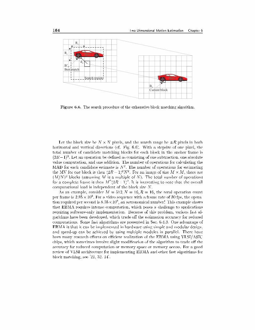
164 Two Dimensional Motion Estimation Chapter 6
Rx
Ry
B’
Best matchm
B
Current blockm
dm
Search region
Figure 6.6. The search procedure of the exhaustive block matching algorithm.
Let the block size be N �N pixels, and the search range be �R pixels in both
horizontal and vertical directions (cf. Fig. 6.6). With a stepsize of one pixel, the
total number of candidate matching blocks for each block in the anchor frame is
(2R+1)2: Let an operation be de�ned as consisting of one subtraction, one absolute
value computation, and one addition. The number of operations for calculating the
MAD for each candidate estimate is N2: The number of operations for estimating
the MV for one block is then (2R+ 1)2N2. For an image of size M �M , there are
(M=N)2 blocks (assuming M is a multiple of N). The total number of operations
for a complete frame is then M2(2R+ 1)2: It is interesting to note that the overall
computational load is independent of the block size N .
As an example, consider M = 512; N = 16; R = 16; the total operation count
per frame is 2:85� 108: For a video sequence with a frame rate of 30 fps, the opera-
tion required per second is 8:55�109, an astronomical number! This example shows
that EBMA requires intense computation, which poses a challenge to applications
requiring software-only implementation. Because of this problem, various fast al-
gorithms have been developed, which trade o� the estimation accuracy for reduced
computations. Some fast algorithms are presented in Sec. 6.4.3. One advantage of
EBMA is that it can be implemented in hardware using simple and modular design,
and speed-up can be achieved by using multiple modules in parallel. There have
been many research e�orts on eÆcient realization of the EBMA using VLSI/ASIC
chips, which sometimes involve slight modi�cation of the algorithm to trade o� the
accuracy for reduced computation or memory space or memory access. For a good
review of VLSI architecture for implementing EBMA and other fast algorithms for
block matching, see [21, 32, 14].
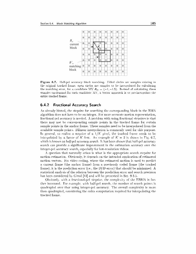
Section 6.4. Block Matching Algorithm 165
Bm:
currentblock
dm
B’m:
matchingblock
Figure 6.7. Half-pel accuracy block matching. Filled circles are samples existing in
the original tracked frame, open circles are samples to be interpolated for calculating
the matching error, for a candidate MV dm = (�1;�1:5). Instead of calculating these
samples on-demand for each candidate MV, a better approach is to pre-interpolate the
entire tracked frame.
6.4.2 Fractional Accuracy Search
As already hinted, the stepsize for searching the corresponding block in the BMA
algorithm does not have to be an integer. For more accurate motion representation,
fractional-pel accuracy is needed. A problem with using fractional stepsizes is that
there may not be corresponding sample points in the tracked frame for certain
sample points in the anchor frame. These samples need to be interpolated from the
available sample points. Bilinear interpolation is commonly used for this purpose.
In general, to realize a stepsize of a 1=K pixel, the tracked frame needs to be
interpolated by a factor of K �rst. An example of K = 2 is shown in Fig. 6.7,
which is known as half-pel accuracy search. It has been shown that half-pel accuracy
search can provide a signi�cant improvement in the estimation accuracy over the
integer-pel accuracy search, especially for low-resolution videos.
A question that naturally arises is what is the appropriate search stepsize for
motion estimation. Obviously, it depends on the intended application of estimated
motion vectors. For video coding, where the estimated motion is used to predict
a current frame (the anchor frame) from a previously coded frame (the tracked
frame), it is the prediction error (i.e., the DFD error) that should be minimized. A
statistical analysis of the relation between the prediction error and search precision
has been considered by Girod [12] and will be presented in Sec. 9.3.5.
Obviously, with a fractional-pel stepsize, the complexity of the EBMA is fur-
ther increased. For example, with half-pel search, the number of search points is
quadrupled over that using integer-pel accuracy. The overall complexity is more
than quadrupled, considering the extra computation required for interpolating the
tracked frame.
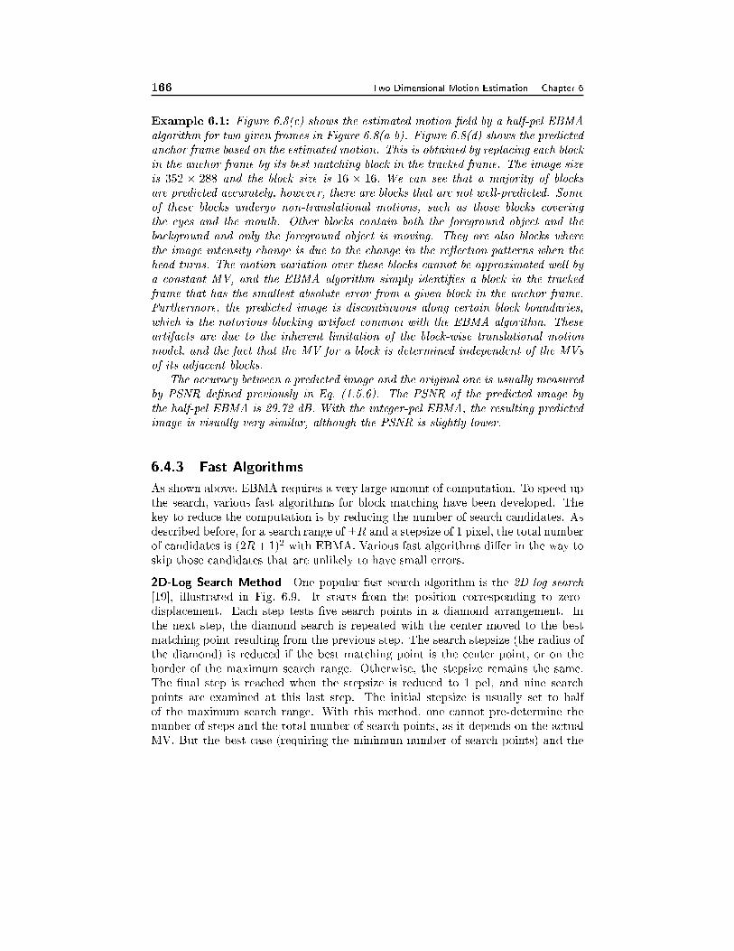
166 Two Dimensional Motion Estimation Chapter 6
Example 6.1: Figure 6.8(c) shows the estimated motion �eld by a half-pel EBMA
algorithm for two given frames in Figure 6.8(a-b). Figure 6.8(d) shows the predicted
anchor frame based on the estimated motion. This is obtained by replacing each block
in the anchor frame by its best matching block in the tracked frame. The image size
is 352 � 288 and the block size is 16 � 16: We can see that a majority of blocks
are predicted accurately, however, there are blocks that are not well-predicted. Some
of these blocks undergo non-translational motions, such as those blocks covering
the eyes and the mouth. Other blocks contain both the foreground object and the
background and only the foreground object is moving. They are also blocks where
the image intensity change is due to the change in the re ection patterns when the
head turns. The motion variation over these blocks cannot be approximated well by
a constant MV, and the EBMA algorithm simply identi�es a block in the tracked
frame that has the smallest absolute error from a given block in the anchor frame.
Furthermore, the predicted image is discontinuous along certain block boundaries,
which is the notorious blocking artifact common with the EBMA algorithm. These
artifacts are due to the inherent limitation of the block-wise translational motion
model, and the fact that the MV for a block is determined independent of the MVs
of its adjacent blocks.
The accuracy between a predicted image and the original one is usually measured
by PSNR de�ned previously in Eq. (1.5.6). The PSNR of the predicted image by
the half-pel EBMA is 29.72 dB. With the integer-pel EBMA, the resulting predicted
image is visually very similar, although the PSNR is slightly lower.
6.4.3 Fast Algorithms
As shown above, EBMA requires a very large amount of computation. To speed up
the search, various fast algorithms for block matching have been developed. The
key to reduce the computation is by reducing the number of search candidates. As
described before, for a search range of �R and a stepsize of 1 pixel, the total number
of candidates is (2R+1)2 with EBMA. Various fast algorithms di�er in the way to
skip those candidates that are unlikely to have small errors.
2D-Log Search Method One popular fast search algorithm is the 2D-log search
[19], illustrated in Fig. 6.9. It starts from the position corresponding to zero-
displacement. Each step tests �ve search points in a diamond arrangement. In
the next step, the diamond search is repeated with the center moved to the best
matching point resulting from the previous step. The search stepsize (the radius of
the diamond) is reduced if the best matching point is the center point, or on the
border of the maximum search range. Otherwise, the stepsize remains the same.
The �nal step is reached when the stepsize is reduced to 1 pel, and nine search
points are examined at this last step. The initial stepsize is usually set to half
of the maximum search range. With this method, one cannot pre-determine the
number of steps and the total number of search points, as it depends on the actual
MV. But the best case (requiring the minimum number of search points) and the
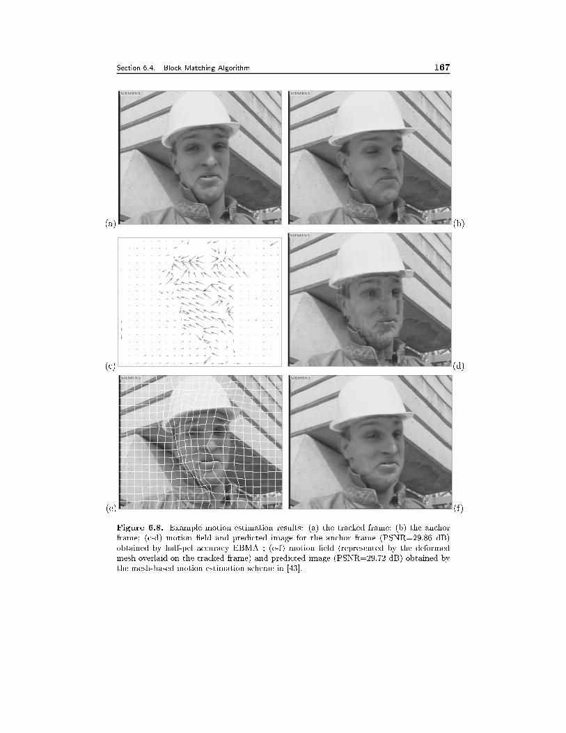
Section 6.4. Block Matching Algorithm 167
(a) (b)
(c) (d)
(e) (f)
Figure 6.8. Example motion estimation results: (a) the tracked frame; (b) the anchor
frame; (c-d) motion �eld and predicted image for the anchor frame (PSNR=29.86 dB)
obtained by half-pel accuracy EBMA ; (e-f) motion �eld (represented by the deformed
mesh overlaid on the tracked frame) and predicted image (PSNR=29.72 dB) obtained by
the mesh-based motion estimation scheme in [43].
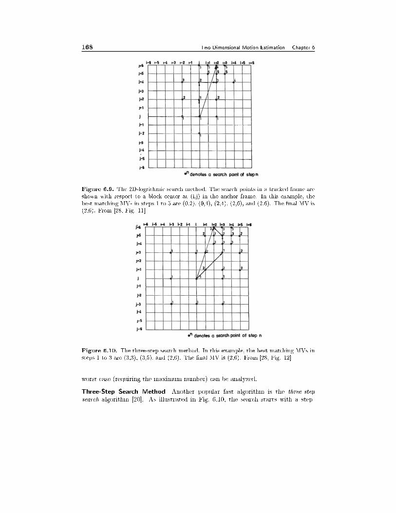
168 Two Dimensional Motion Estimation Chapter 6
Figure 6.9. The 2D-logrithmic search method. The search points in a tracked frame are
shown with respect to a block center at (i,j) in the anchor frame. In this example, the
best matching MVs in steps 1 to 5 are (0,2), (0,4), (2,4), (2,6), and (2,6). The �nal MV is
(2,6). From [28, Fig. 11]
Figure 6.10. The three-step search method. In this example, the best matching MVs in
steps 1 to 3 are (3,3), (3,5), and (2,6). The �nal MV is (2,6). From [28, Fig. 12]
worst case (requiring the maximum number) can be analyzed.
Three-Step Search Method Another popular fast algorithm is the three-step
search algorithm [20]. As illustrated in Fig. 6.10, the search starts with a step-
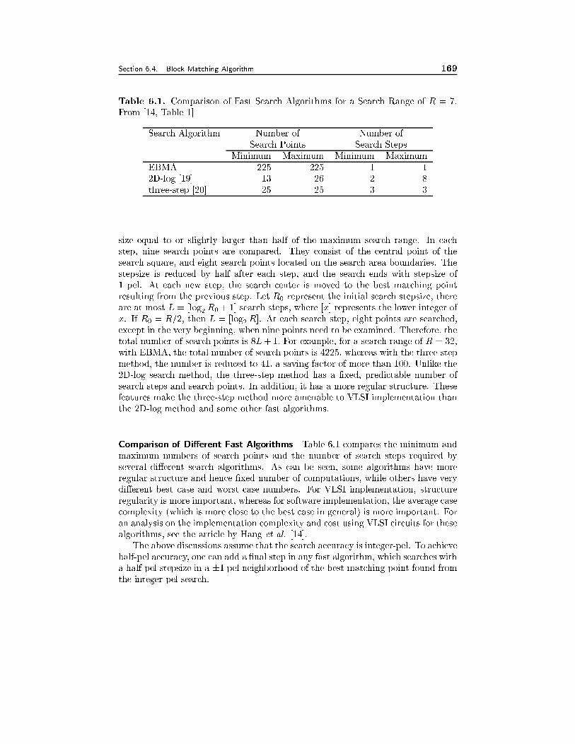
Section 6.4. Block Matching Algorithm 169
Table 6.1. Comparison of Fast Search Algorithms for a Search Range of R = 7.
From [14, Table 1]
Search Algorithm Number of Number of
Search Points Search Steps
Minimum Maximum Minimum Maximum
EBMA 225 225 1 1
2D-log [19] 13 26 2 8
three-step [20] 25 25 3 3
size equal to or slightly larger than half of the maximum search range. In each
step, nine search points are compared. They consist of the central point of the
search square, and eight search points located on the search area boundaries. The
stepsize is reduced by half after each step, and the search ends with stepsize of
1 pel. At each new step, the search center is moved to the best matching point
resulting from the previous step. Let R0 represent the initial search stepsize, there
are at most L = [log2 R0+1] search steps, where [x] represents the lower integer of
x. If R0 = R=2, then L = [log2R]. At each search step, eight points are searched,
except in the very beginning, when nine points need to be examined. Therefore, the
total number of search points is 8L+1: For example, for a search range of R = 32;
with EBMA, the total number of search points is 4225, whereas with the three-step
method, the number is reduced to 41; a saving factor of more than 100. Unlike the
2D-log search method, the three-step method has a �xed, predictable number of
search steps and search points. In addition, it has a more regular structure. These
features make the three-step method more amenable to VLSI implementation than
the 2D-log method and some other fast algorithms.
Comparison of Di�erent Fast Algorithms Table 6.1 compares the minimum and
maximum numbers of search points and the number of search steps required by
several di�erent search algorithms. As can be seen, some algorithms have more
regular structure and hence �xed number of computations, while others have very
di�erent best case and worst case numbers. For VLSI implementation, structure
regularity is more important, whereas for software implementation, the average case
complexity (which is more close to the best case in general) is more important. For
an analysis on the implementation complexity and cost using VLSI circuits for these
algorithms, see the article by Hang et al. [14].
The above discussions assume that the search accuracy is integer-pel. To achieve
half-pel accuracy, one can add a �nal step in any fast algorithm, which searches with
a half-pel stepsize in a �1 pel neighborhood of the best matching point found from
the integer-pel search.
170 Two Dimensional Motion Estimation Chapter 6
6.4.4 Imposing Motion Smoothness Constraints
From Figures 6.8(c), we see that the motion �eld obtained using EBMA is quite
chaotic. This is because no constraints are imposed on the spatial variation of
the block MVs. Several approaches have been developed to make the estimated
motion �eld smoother so that it is closer to the physical motion �eld. One e�ective
approach is to use a hierarchical approach, which estimates the MVs in a coarser
spatial resolution �rst, and then continuously re�ne the MVs in successive �ner
resolutions. The propagation of the MVs from a coarser resolution to a �ner one
is accomplished by spatial interpolation, which induces a certain degree of spatial
continuity on the resulting motion �eld. This technique will be treated in more
detail in Sec. 6.9. Another approach is to explicitly impose a smoothness constraint
by adding a smoothing term in the error criterion in Eq. (6.4.2), which measures the
variation of the MVs of adjacent blocks. The resulting overall error function will be
similar to that in Eq. (6.2.9), except that the motion vectors are de�ned over blocks
and the prediction error is summed over a block. The challenge is to determine a
proper weighting between the prediction error term and the smoothing term so that
the resulting motion �eld is not over-smoothed. Ideally, the weighting should be
adaptive: it should not be applied near object boundaries. A more diÆcult task is
to identify object boundaries where motion discontinuity should be allowed.
6.4.5 Phase Correlation Method�
Instead of minimizing the DFD, another motion estimation method is by identifying
peaks in the phase-correlation function. Assume that two image frames are related
by a pure translation, so that
1(x) = 2(x+ d): (6.4.3)
Taking the Fourier transform on both sides and using the Fourier shift theorem, we
get
1(f) = 2(f) � ej2�dT f : (6.4.4)
The normalized cross power spectrum between 1(x) and 2(x) is
~(f) =1(f) �
�2(f)
j1(f) ��2(f)j
= ej2�dTf ; (6.4.5)
where the superscript � indicates complex conjugation. Taking the inverse Fourier
transform results in the phase correlation function (PCF):4
PCF(x) = F�1f~(f)g = Æ(x + d): (6.4.6)
4The name comes from the fact that it is the cross correlation between the phase portions of
the functions 1(x) and 2(x), respectively.
Section 6.4. Block Matching Algorithm 171
We see that the PCF between two images that are translation of each other is an
impulse function, with the impulse located at a position exactly equal to the trans-
lation between the two images. By identifying the peak location of the PCF, one
can estimate the translation between two images. This approach was �rst used by
Kuglin [23] for image alignment.
The above derivation assumes that both images are continuous in space and have
in�nite size. On the other hand, the actual image signal is discrete and �nite. In
practice, we apply DSFT over the available image domain, which is equivalent to the
periodic extension of the CSFT over an in�nite image that is zero outside the given
image domain (see Secs. 2.1 and 2.2). In order to suppress the aliasing e�ect caused
by sampling, a frequency-domain weighting function W (f) is usually applied when
computing (6.4.5). In [13], a Kaiser window with � = 0:2 is used as the weighting
function. To reduce the e�ect of boundary samples, a space domain weighting
function w(x) can also be applied to 1(x); 2(x) before computing DSFT.
Phase correlation is used extensively in image registration, where entire images
have to be aligned [33][10]. For motion estimation, the underlying two frames are
usually not related by a global translation. To handle this situation, the phase
correlation method is more often applied at the block level. For motion estimation
over non-overlapping blocks of size N � N , both frames are usually divided into
overlapping range blocks of size L� L. For a search range of �R, the range blocksize should be L � N +2R. To determine the MV of a block in 1(x), a size L�Ldiscrete Fourier transform (DFT) is applied to both this block and its corresponding
block in 2(x). Then the PCF is computed using inverse DFT of the same size, and
the peak location is identi�ed. To enable the use of fast Fourier transform (FFT)
algorithms, L is usually chosen to be a power of 2. For example, if N = 16; R = 16,
L = 64 would be appropriate.
The above method assumes that there is a global translation between the two
corresponding range blocks. This assumption does not hold for general video se-
quences. When there are several patches in the range block in 1(x) that undergo
di�erent motions, we will observe several peaks in the PCF. Each peak corresponds
to the motion of one patch. The location of the peak indicates the MV of the patch,
whereas the amplitude of the peak is proportional to the size of the patch [40]. In
this sense, the PCF reveals similar information as the MV histogram over a block.
To estimate the dominant MV of the block, we �rst extract local maxima of the
PCF. We then examine the DFD at the corresponding MV's. The MV yielding
the minimum DFD will be considered the block MV. Since only a small number of
candidate MV's are examined, signi�cant savings in computational complexity may
be achieved compared to the full-search method.
This approach can be extended to motion estimation with fractional pel accu-
racy. In [13], the integer-pel candidate motion vectors are augmented by varying the
length of the candidate motion vectors by up to �1 pel. In [37] and [40], alternativemethods are suggested.
An advantage of the phase correlation method for motion estimation is its in-
sensitivity to illumination changes (see Sec. 5.2). This is because changes in the
172 Two Dimensional Motion Estimation Chapter 6
mean value of an image or multiplication of an image with a constant do not a�ect
the phase information. This is not true for the DFD-based methods.
6.4.6 Binary Feature Matching�
In this scheme, known as Hierarchical Feature Matching Motion Estimation Scheme
(HFM-ME) [25], a Sign Truncated Feature (STF) is de�ned and used for block
template matching, as opposed to the pixel intensity values used in conventional
block matching methods. Using the STF de�nition, a data block is represented
by a mean and a binary bit pattern. The block matching motion estimation is
divided to mean matching and binary phase matching. This technique enables a
signi�cant reduction in computational complexity compared with EBMA because
binary phase matching only involves Boolean logic operation. The use of STF also
signi�cantly reduces the data transfer time between the frame bu�er and motion
estimator. Tests have shown that HFM-ME can achieve similar prediction accuracy
as EBMA under the same search ranges, but can be implemented about 64 times
faster. When the search range is doubled for HFM-ME, it can achieve signi�cantly
more accurate prediction than EBMA, still with nontrivial time savings [25].
The STF vector of a block of size 2Nx2N consists of two parts. The �rst part is
the multiresolution mean vectors, and the second part is the sign-truncated binary
vectors. The mean vectors are determined recursively as follows
Meann(i; j) =
j14
P1
p=0
P1
q=0Meann+1(2i + p; 2j + q)
k; 0 � i; j � 2n � 1; 0 � n � N � 1;
MeanN (i; j) = (i; j); 0 � i; j � 2N � 1;(6.4.7)
where f (i; j); 0 � i; j � 2N�1g are the pixel intensity values of the original block.The sign-truncated vectors are obtained by
ST patternn(i; j) =
�0 if Meann(i; j) � Meann�1(b i
2c; b j
2c);
1 otherwise:(6.4.8)
The STF vectors, decomposed to the n-th level for a 2Nx2N block can then be
represented as
STFVNn= fST patternN; ST patternN�1; :::ST patternN�n+1;meanN�ng: (6.4.9)
When n=N, a block is fully decomposed with the following STF vector
STFVNN = fST patternN; ST patternN�1; :::ST pattern1;mean0g: (6.4.10)
All the intermediate mean vectors are only used to generate ST patterns and can
be discarded. Therefore, the �nal STF representation consists of a multiresolution
binary sequence with 43(4N � 1) bits and a one-byte mean. This represents a much
reduced data set compared to the original 4N bytes of pixel values. Also, this feature
set allows binary Boolean operation for the block matching purpose.
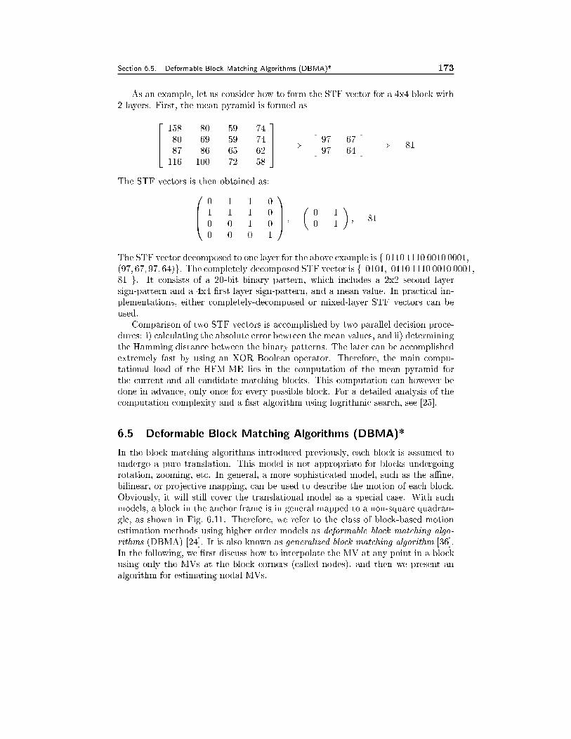
Section 6.5. Deformable Block Matching Algorithms (DBMA)* 173
As an example, let us consider how to form the STF vector for a 4x4 block with
2 layers. First, the mean pyramid is formed as
2664
158 80 59 74
80 69 59 74
87 86 65 62
116 100 72 58
3775 =)
�97 67
97 64
�=) 81
The STF vectors is then obtained as:0BB@
0 1 1 0
1 1 1 0
0 0 1 0
0 0 0 1
1CCA ;
�0 1
0 1
�; 81
The STF vector decomposed to one layer for the above example is f 0110 1110 0010 0001,(97; 67; 97; 64)g. The completely-decomposed STF vector is f 0101, 0110 1110 0010 0001,
81 g. It consists of a 20-bit binary pattern, which includes a 2x2 second layer
sign-pattern and a 4x4 �rst layer sign-pattern, and a mean value. In practical im-
plementations, either completely-decomposed or mixed-layer STF vectors can be
used.
Comparison of two STF vectors is accomplished by two parallel decision proce-
dures: i) calculating the absolute error bewteen the mean values, and ii) determining
the Hamming distance between the binary patterns. The later can be accomplished
extremely fast by using an XOR Boolean operator. Therefore, the main compu-
tational load of the HFM-ME lies in the computation of the mean pyramid for
the current and all candidate matching blocks. This computation can however be
done in advance, only once for every possible block. For a detailed analysis of the
computation complexity and a fast algorithm using logrithmic search, see [25].
6.5 Deformable Block Matching Algorithms (DBMA)*
In the block matching algorithms introduced previously, each block is assumed to
undergo a pure translation. This model is not appropriate for blocks undergoing
rotation, zooming, etc. In general, a more sophisticated model, such as the aÆne,
bilinear, or projective mapping, can be used to describe the motion of each block.
Obviously, it will still cover the translational model as a special case. With such
models, a block in the anchor frame is in general mapped to a non-square quadran-
gle, as shown in Fig. 6.11. Therefore, we refer to the class of block-based motion
estimation methods using higher order models as deformable block matching algo-
rithms (DBMA) [24]. It is also known as generalized block matching algorithm [36].
In the following, we �rst discuss how to interpolate the MV at any point in a block
using only the MVs at the block corners (called nodes), and then we present an
algorithm for estimating nodal MVs.
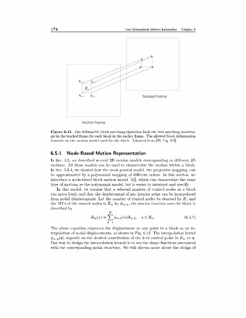
174 Two Dimensional Motion Estimation Chapter 6
xm, 1
xm, 3
xm, 4
xm, 2
Bm
Anchor Frame
Tracked Frame
Figure 6.11. The deformable block matching algorithm �nds the best matching quadran-
gle in the tracked frame for each block in the anchor frame. The allowed block deformation
depends on the motion model used for the block. Adapted from [39, Fig. 6.9].
6.5.1 Node-Based Motion Representation
In Sec. 5.5, we described several 2D motion models corresponding to di�erent 3D
motions. All these models can be used to characterize the motion within a block.
In Sec. 5.5.4, we showed how the most general model, the projective mapping, can
be approximated by a polynomial mapping of di�erent orders. In this section, we
introduce a node-based block motion model [24], which can characterize the same
type of motions as the polynomial model, but is easier to interpret and specify.
In this model, we assume that a selected number of control nodes in a block
can move freely and that the displacement of any interior point can be interpolated
from nodal displacements. Let the number of control nodes be denoted by K, and
the MVs of the control nodes in Bm by dm;k, the motion function over the block is
described by
dm(x) =
KXk=1
�m;k(x)dm;k; x 2 Bm: (6.5.1)
The above equation expresses the displacement at any point in a block as an in-
terpolation of nodal displacements, as shown in Fig. 6.12. The interpolation kernel
�m;k(x) depends on the desired contribution of the k-th control point in Bm to x.
One way to design the interpolation kernels is to use the shape functions associated
with the corresponding nodal structure. We will discuss more about the design of
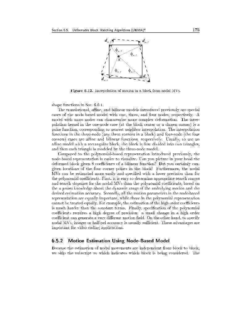
Section 6.5. Deformable Block Matching Algorithms (DBMA)* 175
dm, 1
x
�m, 1
�m, 2
�m, 4
�m, 3
dm, 4
dm, 2dm, 3
Figure 6.12. Interpolation of motion in a block from nodal MVs.
shape functions in Sec. 6.6.1.
The translational, aÆne, and bilinear models introduced previously are special
cases of the node-based model with one, three, and four nodes, respectively. A
model with more nodes can characterize more complex deformation. The inter-
polation kernel in the one-node case (at the block center or a chosen corner) is a
pulse function, corresponding to nearest neighbor interpolation. The interpolation
functions in the three-node (any three corners in a block) and four-node (the four
corners) cases are aÆne and bilinear functions, respectively. Usually, to use an
aÆne model with a rectangular block, the block is �rst divided into two triangles,
and then each triangle is modeled by the three-node model.
Compared to the polynomial-based representation introduced previously, the
node-based representation is easier to visualize. Can you picture in your head the
deformed block given 8 coeÆcients of a bilinear function? But you certainly can,
given locations of the four corner points in the block! Furthermore, the nodal
MVs can be estimated more easily and speci�ed with a lower precision than for
the polynomial coeÆcients. First, it is easy to determine appropriate search ranges
and search stepsizes for the nodal MVs than the polynomial coeÆcients, based on
the a priori knowledge about the dynamic range of the underlying motion and the
desired estimation accuracy. Secondly, all the motion parameters in the node-based
representation are equally important, while those in the polynomial representation
cannot be treated equally. For example, the estimation of the high order coeÆcients
is much harder than the constant terms. Finally, speci�cation of the polynomial
coeÆcients requires a high degree of precision: a small change in a high order
coeÆcient can generate a very di�erent motion �eld. On the other hand, to specify
nodal MVs, integer or half-pel accuracy is usually suÆcient. These advantages are
important for video coding applications.
6.5.2 Motion Estimation Using Node-Based Model
Because the estimation of nodal movements are independent from block to block,
we skip the subscript m which indicates which block is being considered. The
176 Two Dimensional Motion Estimation Chapter 6
following derivation applies to any block B: With the node-based motion model,
the motion parameters for any block are the nodal MVs, i.e., a = [dk; k 2 K];where K = f1; 2; : : : ;Kg: They can be estimated by minimizing the prediction errorover this block, i.e.,
E(a) =Xx2B
j 2(w(x; a)) � 1(x)jp; (6.5.2)
where
w(x; a) = x+Xk2K
�k(x)dk : (6.5.3)
As with the BMA, there are many ways to minimize the error in Eq. (6.5.2),
including exhaustive search and a variety of gradient-based search method. The
computational load required of the exhaustive search, however, can be unacceptable
in practice, because of the high dimension of the search space. Gradient-based
search algorithms are more feasible in this case. In the following, we derive a
Newton-Ralphson search algorithm, following the approach in [24].
De�ne a = [aTx ; aTy ]T with ax = [dx;1; dx;2; : : : ; dx;K ]
T ; ay = [dy;1; dy;2; : : : ; dy;K ]T :
One can show that
@E
@a(a) =
�@E
@ax(a);
@E
@ay(a)
�T;
with
@E
@ax(a) = 2
Xx2B
e(x; a)@ 2(w(x; a))
@x�(x);
@E
@ay(a) = 2
Xx2B
e(x; a)@ 2(w(x; a))
@y�(x):
In the above equations, e(x; a) = 2(w(x; a))� 1(x) and �(x) = [�1(x); �2(x); : : : ; �K(x)]T :
By dropping the terms involving second order gradients, the Hessian matrix can be
approximated as
[H(a)] =
�Hxx(a) Hxy(a)
Hxy(a) Hyy(a)
�;
with
Hxx(a) = 2Xx2B
�@ 2
@x
�2�����w(x;a)
�(x)�(x)T ;
Hyy(a) = 2Xx2B
�@ 2
@y
�2�����w(x;a)
�(x)�(x)T :
Hxy(a) = 2Xx2B
@ 2
@x
@ 2
@y
����w(x;a)
�(x)�(x)T :
Section 6.6. Mesh-Based Motion Estimation� 177
The Newton-Ralphson update algorithm is:
al+1 = al � �[H(al)]�1@E
@a(al): (6.5.4)
The update at each iteration thus requires the inversion of the 2K� 2K symmetric
matrix [H].
To reduce numerical computations, we can update the displacements in x and
y directions separately. Similar derivation will yield:
al+1x
= alx� �[Hxx(a
l)]�1@E
@ax(al); (6.5.5)
al+1y
= aly� �[Hyy(a
l)]�1@E
@ay(al): (6.5.6)
In this case we only need to invert two K �K matrices in each update. For the
four-node case, [H] is an 8� 8 matrix, while [Hxx], and [Hyy] are 4� 4 matrices.
As with all gradient-based iterative processes, the above update algorithm may
reach a bad local minimum that is far from the global minimum, if the initial solution
is not chosen properly. A good initial solution can often be provided by the EBMA.
For example, consider the four-node model with four nodes at the corners of each
block. One can use the average of the motion vectors of the four blocks attached
to each node as the initial estimate of the MV for that node. This initial estimate
can then be successively updated by using Eq. (6.5.4).
Note that the above algorithm can also be applied to polynomial-based motion
representation. In that case, ax and ay would represent the polynomial coeÆcients
associated with horizontal and vertical displacements, respectively, and �k(�) wouldcorrespond to the elementary polynomial basis functions. However, it is diÆcult to
set the search range for ax and ay and check the feasibility of the resulting motion
�eld.
6.6 Mesh-Based Motion Estimation�
With the block-based model used either in BMA or DBMA, motion parameters in
individual blocks are independently speci�ed. Unless motion parameters of adja-
cent blocks are constrained to vary smoothly, the estimated motion �eld is often
discontinuous and sometimes chaotic, as sketched in Fig. 6.13(a). One way to over-
come this problem is by using mesh-based motion estimation. As illustrated in
Figs. 6.13(b), the anchor frame is covered by a mesh, and the motion estimation
problem is to �nd the motion of each node so that the image pattern within each
element in the anchor frame matches well with that in the corresponding deformed
element in the tracked frame. The motion within each element is interpolated from
nodal MVs. As long as the nodes in the tracked frame still form a feasible mesh,
the mesh-based motion representation is guaranteed to be continuous and thus be
free from the blocking artifacts associated with block-based representation. Another
178 Two Dimensional Motion Estimation Chapter 6
bene�t of the mesh-based representation is that it enables continuous tracking of
the same set of nodes over consecutive frames, which is desirable in applications
requiring object tracking. As shown in Fig. 6.13(c), one can generate a mesh for
an initial frame, and then estimate the nodal motions between every two frames.
At each new frame (the anchor frame), the tracked mesh generated in the previous
step is used, so that the same set of nodes are tracked over all frames. This is
not possible with the block-based representation, because it requires that each new
anchor frame be reset to a partition consisting of regular blocks.
Note that the inherent continuity with the mesh-based representation is not al-
ways desired. The type of motion that can be captured by this representation can be
visualized as the deformation of a rubber-sheet, which is continuous everywhere. In
real-world video sequences, there are often motion discontinuities at object bound-
aries. A more accurate representation would be to use separate meshes for di�erent
objects. As with the block-based representation, the accuracy of the mesh-based
representation depends on the number of nodes. A very complex motion �eld can
be reproduced as long as a suÆcient number of nodes are used. To minimize the
number of nodes required, the mesh should be adapted to the imaged scene, so that
the actual motion within each element is smooth (i.e., can be interpolated accu-
rately from the nodal motions). If a regular, non-adaptive mesh is used, a larger
number of nodes are usually needed to approximate the motion �eld accurately.
In the following, we �rst describe how to specify a motion �eld using a mesh-
based representation. We then present algorithms for estimating nodal motions in
a mesh.
6.6.1 Mesh-Based Motion Representation
With the mesh-based motion representation, the underlying image domain in the
anchor frame is partitioned into non-overlapping polygonal elements. Each element
is de�ned by a few nodes and links between the nodes, as shown in Fig. 6.14. Such a
mesh is also known as a control grid. In the mesh-based representation, the motion
�eld over the entire frame is described by MVs at the nodes only. The MVs at the
interior points of an element are interpolated from the MVs at the nodes of this
element. The nodal MVs are constrained so that the nodes in the tracked frame
still form a feasible mesh, with no ip-over elements.
Let the number of elements and nodes be denoted by M and N respectively,
and the number of nodes de�ning each element by K. For convenience, we de�ne
the following index sets: M = f1; 2; : : : ;Mg;N = f1; 2; : : : ; Ng;K = f1; 2; : : : ;Kg:Let the m-th element and n-th node in frame t (t=1 for the anchor frame and t=2
for the tracked frame) be denoted by Bt;m;m 2M and xt;n; n 2 N ; and the MV of
the n-th node by dn = x2;n � x1;n. The motion �eld in element B1;m is related to
the nodal MVs dn by:
dm(x) =Xk2K
�m;k(x)dn(m;k); x 2 B1;m; (6.6.1)
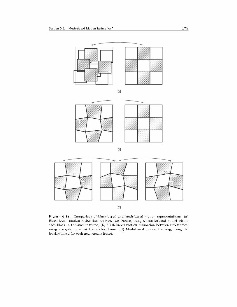
Section 6.6. Mesh-Based Motion Estimation� 179
(a)
(b)
(c)
Figure 6.13. Comparison of block-based and mesh-based motion representations: (a)
Block-based motion estimation between two frames, using a translational model within
each block in the anchor frame; (b) Mesh-based motion estimation between two frames,
using a regular mesh at the anchor frame; (d) Mesh-based motion tracking, using the
tracked mesh for each new anchor frame.
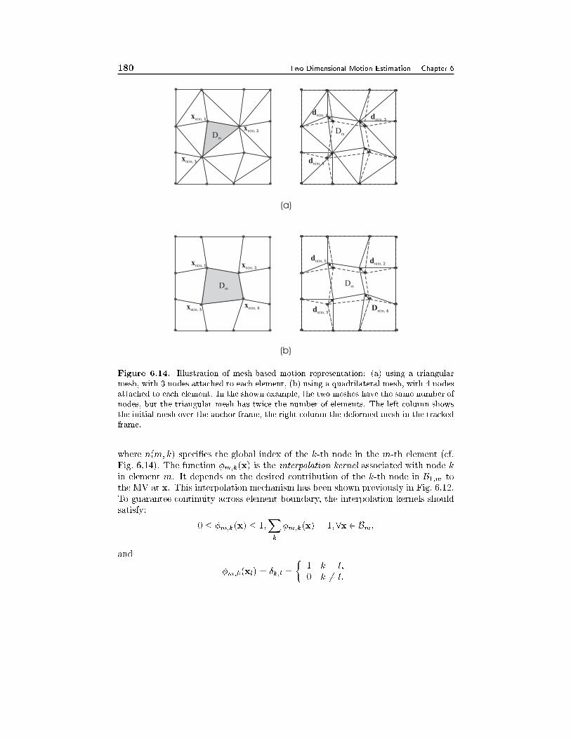
180 Two Dimensional Motion Estimation Chapter 6
(a)
(b)
DmDm
Dm
Dm
xn(m, 1)
xn(m, 1)
dn(m, 1)
dn(m, 1)
xn(m, 2)
xn(m, 2)
dn(m, 2)
dn(m, 2)
Dn(m, 4)xn(m, 4)xn(m, 3)
xn(m, 3) dn(m, 3)
dn(m, 3)
Figure 6.14. Illustration of mesh-based motion representation: (a) using a triangular
mesh, with 3 nodes attached to each element, (b) using a quadrilateral mesh, with 4 nodes
attached to each element. In the shown example, the two meshes have the same number of
nodes, but the triangular mesh has twice the number of elements. The left column shows
the initial mesh over the anchor frame, the right column the deformed mesh in the tracked
frame.
where n(m; k) speci�es the global index of the k-th node in the m-th element (cf.
Fig. 6.14). The function �m;k(x) is the interpolation kernel associated with node k
in element m. It depends on the desired contribution of the k-th node in B1;m to
the MV at x. This interpolation mechanism has been shown previously in Fig. 6.12.
To guarantee continuity across element boundary, the interpolation kernels should
satisfy:
0 � �m;k(x) � 1;Xk
�m;k(x) = 1;8x 2 Bm;
and
�m;k(xl) = Æk;l =
�1 k = l;
0 k 6= l:
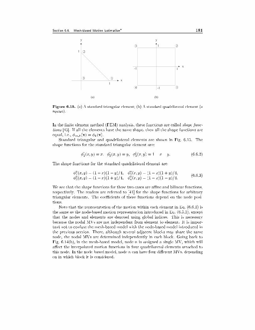
Section 6.6. Mesh-Based Motion Estimation� 181
x
x
y y
1
1
1
1
1
2
2
3
3
4 1
-1
-1
(a) (b)
Figure 6.15. (a) A standard triangular element; (b) A standard quadrilateral element (a
square).
In the �nite element method (FEM) analysis, these functions are called shape func-
tions [45]. If all the elements have the same shape, then all the shape functions are
equal, i.e., �m;k(x) = �k(x):
Standard triangular and quadrilateral elements are shown in Fig. 6.15. The
shape functions for the standard triangular element are:
�t1(x; y) = x; �t2(x; y) = y; �t3(x; y) = 1� x� y: (6.6.2)
The shape functions for the standard quadrilateral element are:
�q
1(x; y) = (1 + x)(1� y)=4; �q
2(x; y) = (1 + x)(1 + y)=4;
�q
3(x; y) = (1� x)(1 + y)=4; �q
4(x; y) = (1� x)(1� y)=4:(6.6.3)
We see that the shape functions for these two cases are aÆne and bilinear functions,
respectively. The readers are referred to [41] for the shape functions for arbitrary
triangular elements. The coeÆcients of these functions depend on the node posi-
tions.
Note that the representation of the motion within each element in Eq. (6.6.1) is
the same as the node-based motion representation introduced in Eq. (6.5.1), except
that the nodes and elements are denoted using global indices. This is necessary
because the nodal MVs are not independent from element to element. It is impor-
tant not to confuse the mesh-based model with the node-based model introduced in
the previous section. There, although several adjacent blocks may share the same
node, the nodal MVs are determined independently in each block. Going back to
Fig. 6.14(b), in the mesh-based model, node n is assigned a single MV, which will
a�ect the interpolated motion functions in four quadrilateral elements attached to
this node. In the node-based model, node n can have four di�erent MVs, depending
on in which block it is considered.
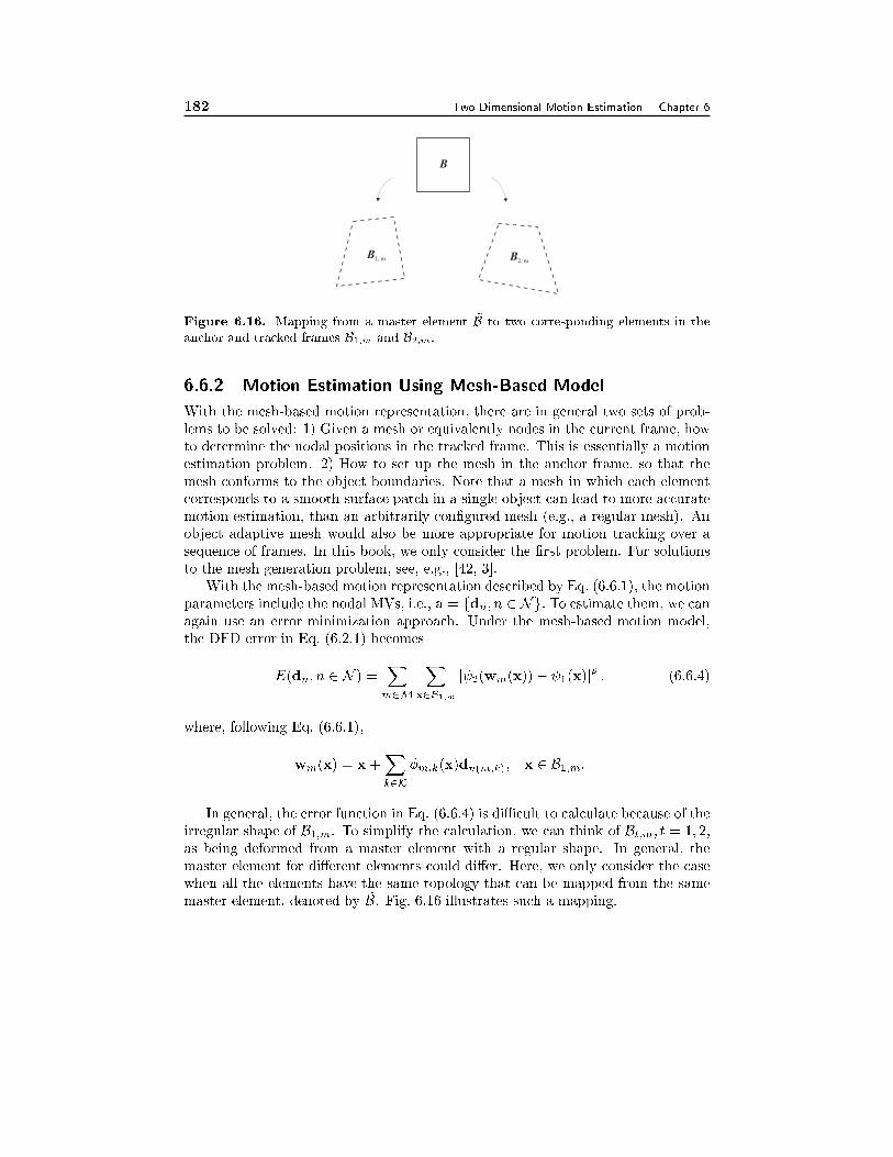
182 Two Dimensional Motion Estimation Chapter 6
B
B1, m B2, m
Figure 6.16. Mapping from a master element ~B to two corresponding elements in the
anchor and tracked frames B1;m and B2;m:
6.6.2 Motion Estimation Using Mesh-Based Model
With the mesh-based motion representation, there are in general two sets of prob-
lems to be solved: 1) Given a mesh or equivalently nodes in the current frame, how
to determine the nodal positions in the tracked frame. This is essentially a motion
estimation problem. 2) How to set up the mesh in the anchor frame, so that the
mesh conforms to the object boundaries. Note that a mesh in which each element
corresponds to a smooth surface patch in a single object can lead to more accurate
motion estimation, than an arbitrarily con�gured mesh (e.g., a regular mesh). An
object adaptive mesh would also be more appropriate for motion tracking over a
sequence of frames. In this book, we only consider the �rst problem. For solutions
to the mesh generation problem, see, e.g., [42, 3].
With the mesh-based motion representation described by Eq. (6.6.1), the motion
parameters include the nodal MVs, i.e., a = fdn; n 2 Ng: To estimate them, we canagain use an error minimization approach. Under the mesh-based motion model,
the DFD error in Eq. (6.2.1) becomes
E(dn; n 2 N ) =Xm2M
Xx2B1;m
j 2(wm(x)) � 1(x)jp; (6.6.4)
where, following Eq. (6.6.1),
wm(x) = x+Xk2K
�m;k(x)dn(m;k); x 2 B1;m:
In general, the error function in Eq. (6.6.4) is diÆcult to calculate because of the
irregular shape of B1;m. To simplify the calculation, we can think of Bt;m; t = 1; 2;
as being deformed from a master element with a regular shape. In general, the
master element for di�erent elements could di�er. Here, we only consider the case
when all the elements have the same topology that can be mapped from the same
master element, denoted by ~B. Fig. 6.16 illustrates such a mapping.
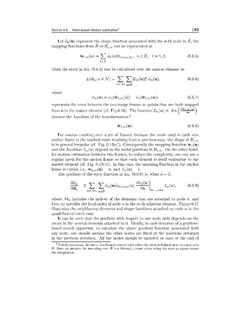
Section 6.6. Mesh-Based Motion Estimation� 183
Let ~�k(u) represent the shape function associated with the k-th node in ~B; themapping functions from ~B to Bt;m can be represented as
~wt;m(u) =Xk2K
~�k(u)xt;n(m;k); u 2 ~B; t = 1; 2; (6.6.5)
Then the error in Eq. (6.6.4) can be calculated over the master element as
E(dn; n 2 N ) =Xm2M
Xu2 ~B
j~em(u)jpJm(u); (6.6.6)
where
~em(u) = 2( ~w2;m(u)) � 1( ~w1;m(u)) (6.6.7)
represents the error between the two image frames at points that are both mapped
from u in the master element (cf. Fig 6.16). The function Jm(u) =���det�@ ~w1;m(u)
@u
����denotes the Jacobian of the transformation:5
~w1;m(u): (6.6.8)
For motion tracking over a set of frames, because the mesh used in each new
anchor frame is the tracked mesh resulting from a previous step, the shape of B1;mis in general irregular (cf. Fig. 6.13(c)). Consequently the mapping function ~w1(u)
and the Jocobian Jm(u) depend on the nodal positions in B1;m. On the other hand,for motion estimation between two frames, to reduce the complexity, one can use a
regular mesh for the anchor frame so that each element is itself equivalent to the
master element (cf. Fig. 6.13(b)). In this case, the mapping function in the anchor
frame is trivial, i.e., w1;m(u) = u, and Jm(u) = 1.
The gradient of the error function in Eq. (6.6.6) is, when p = 2,
@Ep
@dn= 2
Xm2Mn
Xu2 ~B
~em(u)~�k(m;n)(u)@ 2(x)
@x
����~w2;m(u)
Jm(u); (6.6.9)
where Mn includes the indices of the elements that are attached to node n, and
k(m;n) speci�es the local index of node n in the m-th adjacent element. Figure 6.17
illustrates the neighboring elements and shape functions attached to node n in the
quadrilateral mesh case.
It can be seen that the gradient with respect to one node only depends on the
errors in the several elements attached to it. Ideally, in each iteration of a gradient-
based search algorithm, to calculate the above gradient function associated with
any node, one should assume the other nodes are �xed at the positions obtained
in the previous iteration. All the nodes should be updated at once at the end of
5Strictly speaking, the use of Jacobian is correct only when the error is de�ned as an integral over~B. Here we assume the sampling over ~
B is suÆciently dense when using the sum to approximate
the integration.
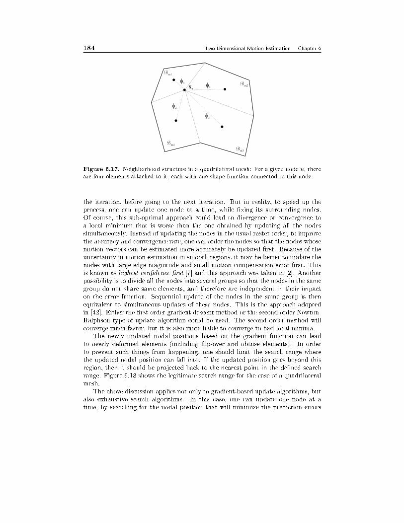
184 Two Dimensional Motion Estimation Chapter 6
xn
Bm1
�1
�2
�3
�4Bm2
Bm3
Bm4
Figure 6.17. Neighborhood structure in a quadrilateral mesh: For a given node n, there
are four elements attached to it, each with one shape function connected to this node.
the iteration, before going to the next iteration. But in reality, to speed up the
process, one can update one node at a time, while �xing its surrounding nodes.
Of course, this sub-optimal approach could lead to divergence or convergence to
a local minimum that is worse than the one obtained by updating all the nodes
simultaneously. Instead of updating the nodes in the usual raster order, to improve
the accuracy and convergence rate, one can order the nodes so that the nodes whose
motion vectors can be estimated more accurately be updated �rst. Because of the
uncertainty in motion estimation in smooth regions, it may be better to update the
nodes with large edge magnitude and small motion compensation error �rst. This
is known as highest con�dence �rst [7] and this approach was taken in [2]. Another
possibility is to divide all the nodes into several groups so that the nodes in the same
group do not share same elements, and therefore are independent in their impact
on the error function. Sequential update of the nodes in the same group is then
equivalent to simultaneous updates of these nodes. This is the approach adopted
in [42]. Either the �rst order gradient descent method or the second order Newton-
Ralphson type of update algorithm could be used. The second order method will
converge much faster, but it is also more liable to converge to bad local minima.
The newly updated nodal positions based on the gradient function can lead
to overly deformed elements (including ip-over and obtuse elements). In order
to prevent such things from happening, one should limit the search range where
the updated nodal position can fall into. If the updated position goes beyond this
region, then it should be projected back to the nearest point in the de�ned search
range. Figure 6.18 shows the legitimate search range for the case of a quadrilateral
mesh.
The above discussion applies not only to gradient-based update algorithms, but
also exhaustive search algorithms. In this case, one can update one node at a
time, by searching for the nodal position that will minimize the prediction errors
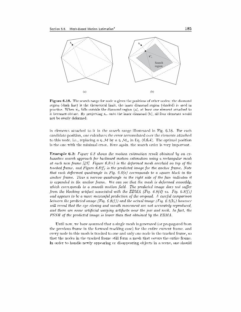
Section 6.6. Mesh-Based Motion Estimation� 185
xn xn
x’n
Searchregion
(a) (b)
Figure 6.18. The search range for node n given the positions of other nodes: the diamond
region (dash line) is the theoretical limit, the inner diamond region (shaded) is used in
practice. When xn falls outside the diamond region (a), at least one element attached to
it becomes obtuse. By projecting xn onto the inner diamond (b), all four elements would
not be overly deformed.
in elements attached to it in the search range illustrated in Fig. 6.18. For each
candidate position, one calculates the error accumulated over the elements attached
to this node, i.e., replacing n 2M by n 2Mn in Eq. (6.6.4). The optimal position
is the one with the minimal error. Here again, the search order is very important.
Example 6.2: Figure 6.8 shows the motion estimation result obtained by an ex-
haustive search approach for backward motion estimation using a rectangular mesh
at each new frame [43]. Figure 6.8(e) is the deformed mesh overlaid on top of the
tracked frame, and Figure 6.8(f) is the predicted image for the anchor frame. Note
that each deformed quadrangle in Fig. 6.8(e) corresponds to a square block in the
anchor frame. Thus a narrow quadrangle in the right side of the face indicates it
is expanded in the anchor frame. We can see that the mesh is deformed smoothly,
which corresponds to a smooth motion �eld. The predicted image does not su�er
from the blocking artifact associated with the EBMA (Fig. 6.8(d) vs. Fig. 6.8(f))
and appears to be a more successful prediction of the original. A careful comparison
between the predicted image (Fig. 6.8(f)) and the actual image (Fig. 6.8(b)) however
will reveal that the eye closing and mouth movement are not accurately reproduced,
and there are some arti�cial warping artifacts near the jaw and neck. In fact, the
PSNR of the predicted image is lower than that obtained by the EBMA.
Until now, we have assumed that a single mesh is generated (or propagated from
the previous frame in the forward tracking case) for the entire current frame, and
every node in this mesh is tracked to one and only one node in the tracked frame, so
that the nodes in the tracked frame still form a mesh that covers the entire frame.
In order to handle newly appearing or disappearing objects in a scene, one should
186 Two Dimensional Motion Estimation Chapter 6
allow the deletion of nodes corresponding to disappeared objects, and creation of
new nodes in newly appearing objects. For a solution to such problem, see [3].
6.7 Global Motion Estimation
In Sec. 5.5, we showed that, depending on the camera and object motion and the
object surface geometry, the mapping function between the two images of the same
imaged object can be described by a translation, a geometric transformation, an
aÆne mapping, or a projective mapping. Such a model can be applied to the entire
frame if the entire motion �eld is caused by a camera motion, or if the imaged scene
consists of a single object that is undergoing a rigid 3D motion.6
In practice, one can hardly �nd a video sequence that contains a single object.
There are usually at least two objects: a stationary background and a moving
foreground. More often, there are more than one foreground objects. Fortunately,
when the foreground object motion is small compared to the camera motion, and
the camera does not move in the Z-direction, the motion �eld can be approximated
well by a global model. This will be the case, for example, when the camera pans
over a scene or zooms into a particular subject in a relatively fast speed. Such
camera motions are quite common in sports video and movies. Even when the
actual 2D motion �eld cannot be represented by a single global motion accurately,
as long as the e�ect of the camera motion dominates over other motions (motion of
individual small objects), determination of this dominant global motion is still very
useful. In this section, we discuss the estimation of global motions.
There are in general two approaches for estimating the global motion. One is to
estimate the global motion parameters directly by minimizing the prediction errors
under a given set of motion parameters. The other is to �rst determine pixel-wise or
block-wise motion vectors, using the techniques described previously, and then using
a regression method to �nd the global motion model that best �ts the estimated
motion �eld. The latter method can also be applied to motion vectors at selected
feature points, such as points with strong edges.
6.7.1 Robust Estimator
A diÆculty in estimating the global motion is that a pixel may not experience only
the global motion. Usually, the motion at any pixel can be decomposed into a global
motion (caused by camera movement) and a local motion because of the movement
of the underlying object. Therefore, the prediction error obtained by using the
global motion model alone may not be small, even if the correct global motion
parameters are available. In other instances, not all the pixels in the same frame
experience the global motion and ideally one should not apply the same motion
6Recall that in the case that the camera or the object moves in the Z-direction, the motion
�eld can be represented by a projective mapping only if the object surface is planar. When the
object surfaces is spatially varying, the mapping function at any point also depends on the surface
depth of that point and cannot be represented by a global model.
Section 6.7. Global Motion Estimation 187
model to the entire frame. These problems can be overcome by a robust estimation
method [35], if the global motion is dominant over other local motions, in the sense
that the pixels that experience the same global motion and only the global motion
occupy a signi�cantly larger portion of the underlying image domain than those
pixels that do not.
The basic idea in robust estimation is to consider the pixels that are governed
by the global motion as inliers, and the remaining pixels as outliers. Initially, one
assume that all the pixels undergo the same global motion, and estimate the motion
parameters by minimizing the prediction or �tting error over all the pixels. This
will yield an initial set of motion parameters. With this initial solution, one can
then calculate the prediction or �tting error over each pixel. The pixels where the
errors exceed a certain threshold will be classi�ed as outliers and be eliminated
from the next iteration. The above process is then repeated to the remaining inlier
pixels. This process iterates until no outlier pixels exist. This approach is called
Hard Threshold Robust Estimator.
Rather than simply labeling a pixel as either inlier or outlier at the end of each
iteration, one can also assign a di�erent weight to each pixel, with a large weight
for a pixel with small error, and vice verse. At the next minimization or �tting
iteration, a weighted error measure is used, so that the pixels with larger errors in
the previous iteration will have less impact than those with smaller errors. This
approach is known as Soft Threshold Robust Estimator.
6.7.2 Direct Estimation
In either the hard or soft threshold robust estimator, each iteration involves the
minimization of an error function. Here we derive the form of the function when
the model parameters are directly obtained by minimizing the prediction error. We
only consider the soft-threshold case, as the hard-threshold case can be considered
as a special case where the weights are either one or zero. Let the mapping function
from the anchor frame to the tracked frame be denoted by w(x; a), where a is the
vector that contains all the global motion parameters. The prediction error can be
written as, following Eq. (6.2.1):
EDFD =Xx2�
w(x) j 2(w(x; a)) � 1(x)jp
(6.7.1)
where w(x) are the weighting coeÆcients for pixel x. Within each iteration of
the robust estimation process, the parameter vector a is estimated by minimizing
the above error, using either gradient-based method or exhaustive search. The
weighting factor at x, w(x), in a new iteration will be adjusted based on the DFD
at x calculated based on the motion parameters estimated in the previous iteration.
6.7.3 Indirect Estimation
In this case, we assume that the motion vectors d(x) have been estimated at a set
of suÆciently dense points x 2 �0 � �; where � represent the set of all pixels.
188 Two Dimensional Motion Estimation Chapter 6
This can be accomplished, for example, using either the block-based or mesh-based
approaches described before. One can also choose to estimate the motion vectors at
only selected feature points, where the estimation accuracy is high. The task here is
to determine a so that the model d(x; a) can approximate the pre-estimated motion
vectors d(x);x 2 �0 well. This can be accomplished by minimizing the following
�tting error:
E�tting =Xx2�0
w(x) jd(x; a) � d(x)jp
(6.7.2)
As shown in Sec. 5.5.4, a global motion can usually be described or approximated
by a polynomial function. In this case, a consists of the polynomial coeÆcients and
d(x; a) is a linear function of a, i.e., d(x; a) = [A(x)]a. If we choose p = 2; then the
above minimization problem becomes a weighted least squares problem. By setting@Efitting
@a= 0, we obtain the following solution
a =
Xx2�0
w(x)[A(x)]T [A(x)]
!�1 Xx2�0
w(x)[A(x)]T d(x)
!: (6.7.3)
As an example, consider the aÆne motion model given in Eq. (5.5.16). The
motion parameter vector is a = [a0; a1; a2; b0; b1; b2]T ; and the matrix [A(x)] is
[A(x)] =
�1 x y 0 0 0
0 0 0 1 x y
�:
In fact, the parameters for the x and y dimensions are not coupled and can be
estimated separately, which will reduce the matrix sizes involved. For example, to
estimate the x dimensional parameter ax = [a0; a1; a2], the associated matrix is
[Ax(x)] = [1; x; y], and the solution is:
ax =
Xx2�0
w(x)[Ax(x)]T [Ax(x)]
!�1 Xx2�0
w(x)[Ax(x)]T dx(x)
!: (6.7.4)
6.8 Region-Based Motion Estimation�
As already pointed out in the previous section, there are usually multiple types of
motions in the imaged scene, which correspond to motions associated with di�erent
objects. By region-based motion estimation, we mean to segment the underlying
image frame into multiple regions and estimate the motion parameters of each
region. The segmentation should be such that a single parametric motion model
can represent well the motion in each region. Obviously, region segmentation is
dependent on the motion model used for characterizing each region. The simplest
approach is to require each region undergo the same translational motion. This
requirement however can result in too many small regions, because the 2-D motion
Section 6.8. Region-Based Motion Estimation� 189
in a region corresponding to a physical object can rarely be modeled by a simple
translation. Such a region would have to be split into many small sub-regions
for each sub-region to have a translational motion. For a more eÆcient motion
representation, an aÆne or bilinear or perspective motion model should be used.
In general, there are three approaches for accomplishing region-based motion
estimation. With the �rst approach, one �rst segments the image frame into di�er-
ent regions based on texture homogeneity, the edge information, and sometimes the
motion boundary obtained by analyzing the di�erence image between two frames,
and then estimates the motion in each region. The latter can be accomplished by
applying the global motion estimation method described in Sec. 6.7 to each region.
We call such a method region-�rst. With the second approach, one �rst estimates
the motion �eld over the entire frame, and then segments the resulting motion �eld
so that the motion in each region can be modeled by a single parametric model. We
call this method motion-�rst. The resulting region can be further re�ned subject
to some spatial connectivity constraints. The �rst step can be accomplished using
the various motion estimation methods described previously, including the pixel-,
block-, and mesh-based methods. The second problem involves motion-based seg-
mentation, which is discussed further in Sec. 6.8.1. Yet the third approach is to
jointly estimate region partition and motion in each region. In general, this is ac-
complished by an iterative process, which performs region segmentation and motion
estimation alternatively. This approach is described in Sec. 6.8.2.
6.8.1 Motion-Based Region Segmentation
As described already, motion-based segmentation refers to the partitioning of a
motion �eld into multiple regions so that the motion within each region can be
described by a single set of motion parameters. Here we present two approaches for
accomplishing this task. The �rst approach uses a clustering technique to identify
similar motion vectors. The second approach uses a layered approach to estimate
the underlying region and associated motions sequentially, starting from the region
with the most dominant motion.
Clustering Consider the case when the motion model for each region is a pure
translation. Then the segmentation task is to group all spatially connected pixels
with similar motion vectors into one region. This can be easily accomplished by
an automated clustering method, such as the K-means or the ISODATA method
[8]. This is an iterative process: Starting from an initial partitioning, the mean
motion vector, known as the centroid, of each region is calculated. Then each pixel
is reclassi�ed into the region whose centroid is closest to the motion vector of this
pixel. This results in a new partition and the above two steps can be repeated until
the partition does not change any more. In this process, the spatial connectivity
is not considered. Therefore, the resulting regions may contain pixels that are
not spatially connected. Postprocessing steps may be applied at the end of the
iterations to improve the spatial connectivity of the resulting regions. For example,
a single region may be split into several sub-regions so that each region is a spatially
190 Two Dimensional Motion Estimation Chapter 6
connected subset, isolated pixels may be merged into its surrounding region, and
�nally region boundaries can be smoothed using morphological operators.
When the motion model for each region is not a simple translation, motion-based
clustering is not as straight forward. This is because one cannot use the similarity
between motion vectors as the criterion for performing clustering. One way is to
�nd a set of motion parameters for each pixel by �tting the motion vectors in its
neighborhood into a speci�ed model. Then one can employ the clustering method
described previously, by replacing the raw motion vector with the motion parameter
vector. If the original motion �eld is given in the block-based representation using
a higher order model, then one can cluster blocks with similar motion parameters
into the same region. Similarly, with the mesh-based motion representation, one can
derive a set of motion parameters for each element based on its nodal displacements,
and then clustering the elements with similar parameters into the same region. This
is the parallel approach described in [44].
Layered Approach Very often, the motion �eld in a scene can be decomposed into
layers, with the �rst layer representing the most dominant motion, the second layer
the less dominant one, and so on. Here, the dominance of a motion is determined
by the area of the region undergoing the corresponding motion. The most dominant
motion is often a re ection of the camera motion, which a�ects the entire imaged
domain. For example, in a video clip of a tennis play, the background will be the
�rst layer, which usually undergoes a coherent global camera motion; the player the
second layer (which usually contains several sub-object level motions corresponding
to the movements of di�erent parts of the body), the racket the third, and the
ball the fourth layer. To extract the motion parameters in di�erent layers, one
can use the robust estimator method described in Sec. 6.7.1 recursively. First, we
try to model the motion �eld of the entire frame by a single set of parameters,
and continuously eliminate outlier pixels from the remaining inlier group, until all
the pixels within the inlier group can be modeled well. This will yield the �rst
dominant region (corresponding to the inlier region) and its associated motion.
The same approach can then be applied to the remaining pixels (the outlier region)
to identify the next dominant region and its motion. This process continues until
no more outlier pixels exist. As before, postprocessing may be invoked at the end
of the iterations to improve the spatial connectivity of the resulting regions. This
is the sequential approach described in [44].
For the above scheme to work well, the inlier region must be larger than the
outlier region at any iteration. This means that the largest region must be greater
than the combined area of all other regions, the second largest region must be
greater than the combined area of the remaining regions, and so on. This condition
is satis�ed in most video scenes, which often contain a stationary background that
covers a large portion of the underlying image, and di�erent moving objects with
varying sizes.
Section 6.9. Multi-Resolution Motion Estimation 191
6.8.2 Joint Region Segmentation and Motion Estimation
Theoretically, one can formulate the joint estimation of the region segmentation map
and the motion parameters of each region as an optimization problem. The function
to be minimized could be a combination of the motion compensated prediction
error and a region smoothness measure. The solution of the optimization problem
however is diÆcult because of the very high dimension of the parameter space
and the complicated interdependence between these parameters. In practice, a
sub-optimal approach is often taken, which alternates between the estimation of
the segmentation and motion parameters. Based on an initial segmentation, the
motion of each region is �rst estimated. In the next iteration, the segmentation
is re�ned, e.g., by eliminating outlier pixels in each region where the prediction
errors are large, and by merging pixels sharing similar motion models. The motion
parameters for each re�ned region are then be re-estimated. This process continues
until no more changes in the segmentation map occur.
An alternative approach is to estimate the regions and their associated motions
in a layered manner, similar to the layered approach described previously. There,
we assume that the motion vector at every point is already known, and the identi�-
cation of the region with the most dominant motion (i.e. the inlier) is accomplished
by examining the �tting error induced by representing individual MVs using a set
of motion parameters. This is essentially the indirect robust estimator presented
in Sec. 6.7.3. In the joint region segmentation and motion estimation approach,
to extract the next dominant region and its associated motion from the remaining
pixels, we can use the direct robust estimator. That is, we directly estimate the
motion parameters, by minimizing the prediction errors at these pixels. Once the
parameters are determined, we determine whether a pixel belongs to the inlier by
examining the prediction error at this pixel. We then re-estimate the motion pa-
rameters by minimizing the prediction errors at the inlier pixels only. This approach
has been taken by Hsu [18].
6.9 Multi-Resolution Motion Estimation
As can be seen from previous sections, various motion estimation approaches can be
reduced to solving an error minimization problem. Two major diÆculties associated
with obtaining the correct solution are: i) the minimization function usually has
many local minima and it is not easy to reach the global minimum, unless it is close
to the chosen initial solution; and ii) the amount of computation involved in the
minimization process is very high. Both problems can be combated by the multi-
resolution approach, which searches the solution for an optimization problem in
successively �ner resolutions. By �rst searching the solution in a coarse resolution,
one can usually obtain a solution that is close to the true motion. In addition, by
limiting the search in each �ner resolution to a small neighborhood of the solution
obtained in the previous resolution, the total number of searches can be reduced,
compared to that required by directly searching in the �nest resolution over a large
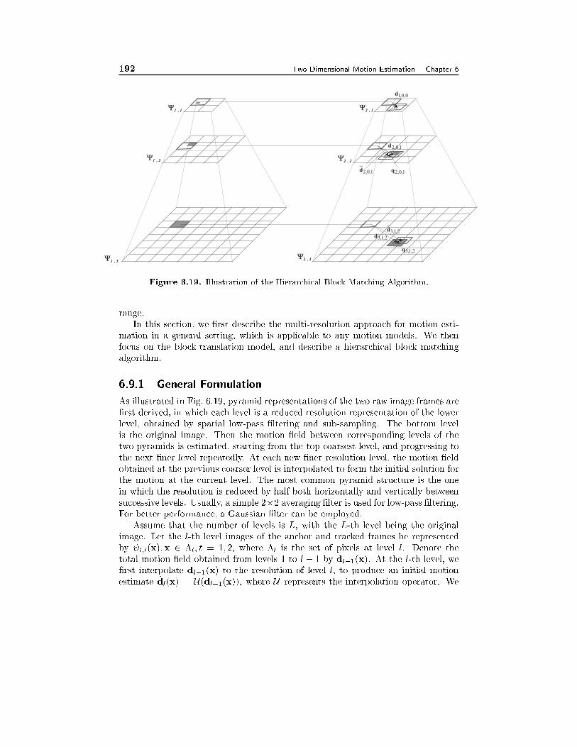
192 Two Dimensional Motion Estimation Chapter 6
�2 , 3�2 , 3
�1 , 2�1 , 2
�1 , 3�1 , 3
�2 , 2�2 , 2
�1 , 1�1 , 1 �2 , 1�2 , 1
1,0,2~d
2,1,3~d
2,1,3q
2,1,3d
1,0,2d
1,0,2q
0,0,1d
Figure 6.19. Illustration of the Hierarchical Block Matching Algorithm.
range.
In this section, we �rst describe the multi-resolution approach for motion esti-
mation in a general setting, which is applicable to any motion models. We then
focus on the block-translation model, and describe a hierarchical block matching
algorithm.
6.9.1 General Formulation
As illustrated in Fig. 6.19, pyramid representations of the two raw image frames are
�rst derived, in which each level is a reduced resolution representation of the lower
level, obtained by spatial low-pass �ltering and sub-sampling. The bottom level
is the original image. Then the motion �eld between corresponding levels of the
two pyramids is estimated, starting from the top coarsest level, and progressing to
the next �ner level repeatedly. At each new �ner resolution level, the motion �eld
obtained at the previous coarser level is interpolated to form the initial solution for
the motion at the current level. The most common pyramid structure is the one
in which the resolution is reduced by half both horizontally and vertically between
successive levels. Usually, a simple 2�2 averaging �lter is used for low-pass �ltering.For better performance, a Gaussian �lter can be employed.
Assume that the number of levels is L, with the L-th level being the original
image. Let the l-th level images of the anchor and tracked frames be represented
by t;l(x);x 2 �l; t = 1; 2; where �l is the set of pixels at level l. Denote the
total motion �eld obtained from levels 1 to l � 1 by dl�1(x). At the l-th level, we
�rst interpolate dl�1(x) to the resolution of level l, to produce an initial motion
estimate ~dl(x) = U(dl�1(x)); where U represents the interpolation operator. We
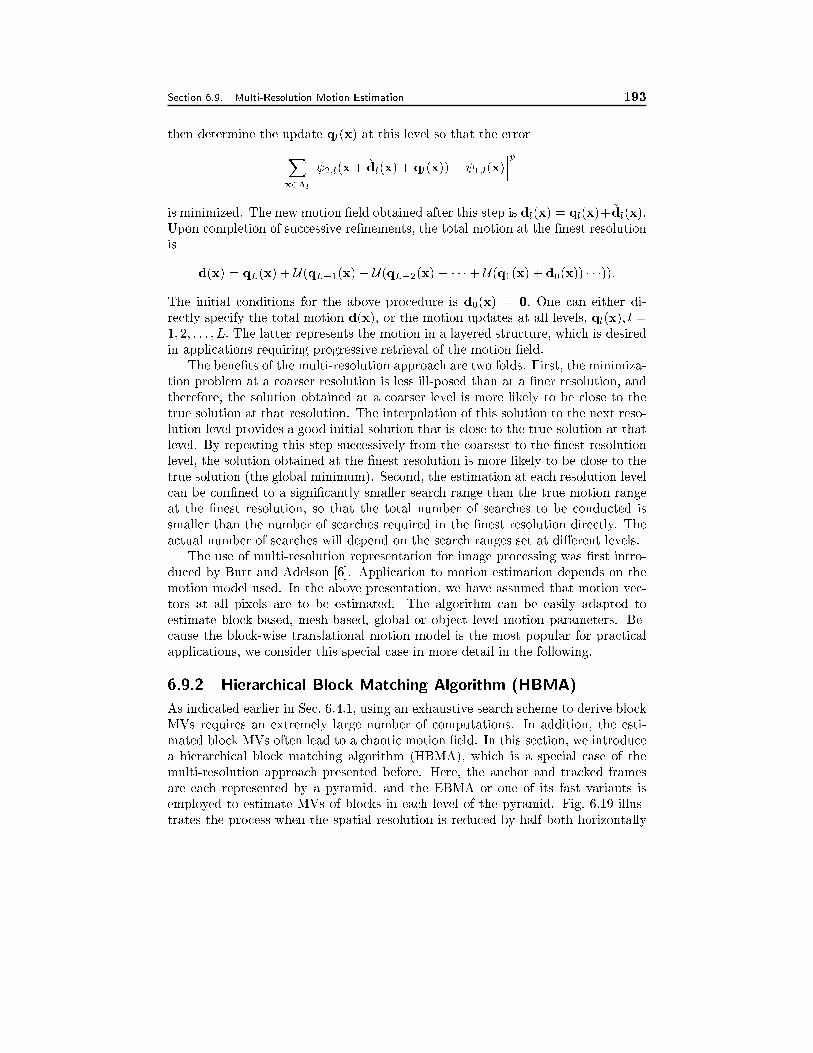
Section 6.9. Multi-Resolution Motion Estimation 193
then determine the update ql(x) at this level so that the errorXx2�l
��� 2;l(x+ ~dl(x) + ql(x)) � 1;l(x)���p
is minimized. The new motion �eld obtained after this step is dl(x) = ql(x)+~dl(x):
Upon completion of successive re�nements, the total motion at the �nest resolution
is
d(x) = qL(x) + U(qL�1(x) + U(qL�2(x) + � � �+ U(q1(x) + d0(x)) � � �)):
The initial conditions for the above procedure is d0(x) = 0: One can either di-
rectly specify the total motion d(x), or the motion updates at all levels, ql(x); l =
1; 2; : : : ; L: The latter represents the motion in a layered structure, which is desired
in applications requiring progressive retrieval of the motion �eld.
The bene�ts of the multi-resolution approach are two folds. First, the minimiza-
tion problem at a coarser resolution is less ill-posed than at a �ner resolution, and
therefore, the solution obtained at a coarser level is more likely to be close to the
true solution at that resolution. The interpolation of this solution to the next reso-
lution level provides a good initial solution that is close to the true solution at that
level. By repeating this step successively from the coarsest to the �nest resolution
level, the solution obtained at the �nest resolution is more likely to be close to the
true solution (the global minimum). Second, the estimation at each resolution level
can be con�ned to a signi�cantly smaller search range than the true motion range
at the �nest resolution, so that the total number of searches to be conducted is
smaller than the number of searches required in the �nest resolution directly. The
actual number of searches will depend on the search ranges set at di�erent levels.
The use of multi-resolution representation for image processing was �rst intro-
duced by Burt and Adelson [6]. Application to motion estimation depends on the
motion model used. In the above presentation, we have assumed that motion vec-
tors at all pixels are to be estimated. The algorithm can be easily adapted to
estimate block-based, mesh-based, global or object level motion parameters. Be-
cause the block-wise translational motion model is the most popular for practical
applications, we consider this special case in more detail in the following.
6.9.2 Hierarchical Block Matching Algorithm (HBMA)
As indicated earlier in Sec. 6.4.1, using an exhaustive search scheme to derive block
MVs requires an extremely large number of computations. In addition, the esti-
mated block MVs often lead to a chaotic motion �eld. In this section, we introduce
a hierarchical block matching algorithm (HBMA), which is a special case of the
multi-resolution approach presented before. Here, the anchor and tracked frames
are each represented by a pyramid, and the EBMA or one of its fast variants is
employed to estimate MVs of blocks in each level of the pyramid. Fig. 6.19 illus-
trates the process when the spatial resolution is reduced by half both horizontally
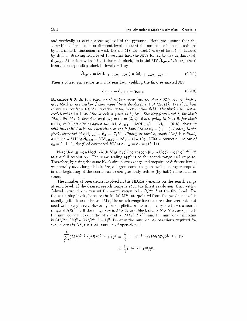
194 Two Dimensional Motion Estimation Chapter 6
and vertically at each increasing level of the pyramid. Here, we assume that the
same block size is used at di�erent levels, so that the number of blocks is reduced
by half in each dimension as well. Let the MV for block (m;n) at level l be denoted
by dl;m;n. Starting from level 1, we �rst �nd the MVs for all blocks in this level,
d1;m;n. At each new level l > 1, for each block, its initial MV ~dl;m;n is interpolated
from a corresponding block in level l � 1 by
~dl;m;n = U(dl�1;bm=2c;bn=2c) = 2dl�1;bm=2c;bn=2c: (6.9.1)
Then a correction vector ql;m;n is searched, yielding the �nal estimated MV
dl;m;n = ~dl;m;n + ql;m;n: (6.9.2)
Example 6.3: In Fig. 6.20, we show two video frames, of size 32� 32, in which a
gray block in the anchor frame moved by a displacement of (13,11). We show how
to use a three level HBMA to estimate the block motion �eld. The block size used at
each level is 4�4, and the search stepsize is 1 pixel. Starting from level 1, for block
(0,0), the MV is found to be d1;0;0 = d1 = (3; 3): When going to level 2, for block
(0; 1), it is initially assigned the MV ~d2;0;1 = U(d1;0;0) = 2d1 = (6; 6): Starting
with this initial MV, the correction vector is found to be q2 = (1;�1), leading to the
�nal estimated MV d2;0;1 = d2 = (7; 5). Finally at level 3, block (1,2) is initially
assigned a MV of ~d3;1;2 = U(d2;0;1) = 2d2 = (14; 10). With a correction vector of
q3 = (�1; 1), the �nal estimated MV is d3;1;2 = d3 = (13; 11):
Note that using a block width N at level l corresponds to a block width of 2L�lN
at the full resolution. The same scaling applies to the search range and stepsize.
Therefore, by using the same block size, search range and stepsize at di�erent levels,
we actually use a larger block size, a larger search range, as well as a larger stepsize
in the beginning of the search, and then gradually reduce (by half) these in later
steps.
The number of operations involved in the HBMA depends on the search range
at each level. If the desired search range is R in the �nest resolution, then with a
L-level pyramid, one can set the search range to be R=2L�1 at the �rst level. For
the remaining levels, because the initial MV interpolated from the previous level is
usually quite close to the true MV, the search range for the correction vector do not
need to be very large. However, for simplicity, we assume every level uses a search
range of R=2L�1. If the image size isM �M and block size is N �N at every level,
the number of blocks at the l-th level is (M=2L�lN)2, and the number of searches
is (M=2L�lN)2 � (2R=2L�1 + 1)2: Because the number of operations required for
each search is N2, the total number of operations is
LXl=1
(M=2L�l)2(2R=2L�1 + 1)2 =4
3(1� 4�(L�1))M2(2R=2L�1 + 1)2
�1
34�(L�2)4M2R2:
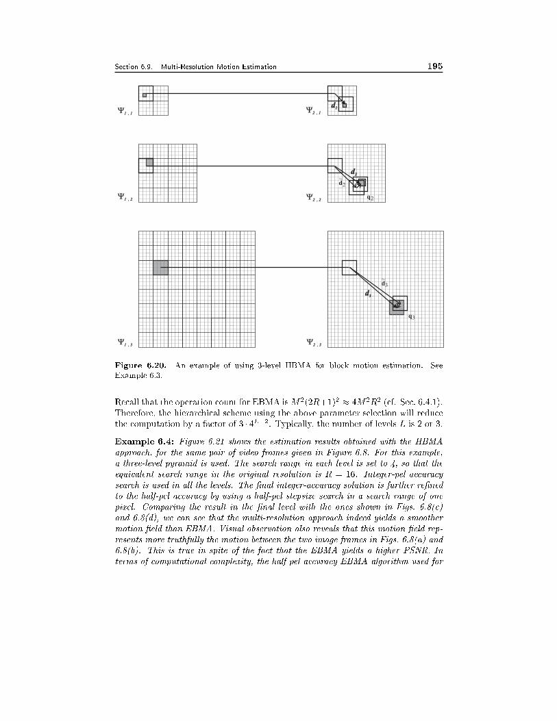
Section 6.9. Multi-Resolution Motion Estimation 195
�2 , 3�2 , 3
�2 , 2�2 , 2
�2 , 1�2 , 1
�1 , 2�1 , 2
�1 , 3�1 , 3
�1 , 1�1 , 1
d1
d1
d3
d3
d2
d2
2~d
3~d
3q
2q
Figure 6.20. An example of using 3-level HBMA for block motion estimation. See
Example 6.3.
Recall that the operation count for EBMA isM2(2R+1)2 � 4M2R2 (cf. Sec. 6.4.1).
Therefore, the hierarchical scheme using the above parameter selection will reduce
the computation by a factor of 3 � 4L�2. Typically, the number of levels L is 2 or 3.
Example 6.4: Figure 6.21 shows the estimation results obtained with the HBMA
approach, for the same pair of video frames given in Figure 6.8. For this example,
a three-level pyramid is used. The search range in each level is set to 4, so that the
equivalent search range in the original resolution is R = 16. Integer-pel accuracy
search is used in all the levels. The �nal integer-accuracy solution is further re�ned
to the half-pel accuracy by using a half-pel stepsize search in a search range of one
pixel. Comparing the result in the �nal level with the ones shown in Figs. 6.8(c)
and 6.8(d), we can see that the multi-resolution approach indeed yields a smoother
motion �eld than EBMA. Visual observation also reveals that this motion �eld rep-
resents more truthfully the motion between the two image frames in Figs. 6.8(a) and
6.8(b). This is true in spite of the fact that the EBMA yields a higher PSNR. In
terms of computational complexity, the half-pel accuracy EBMA algorithm used for
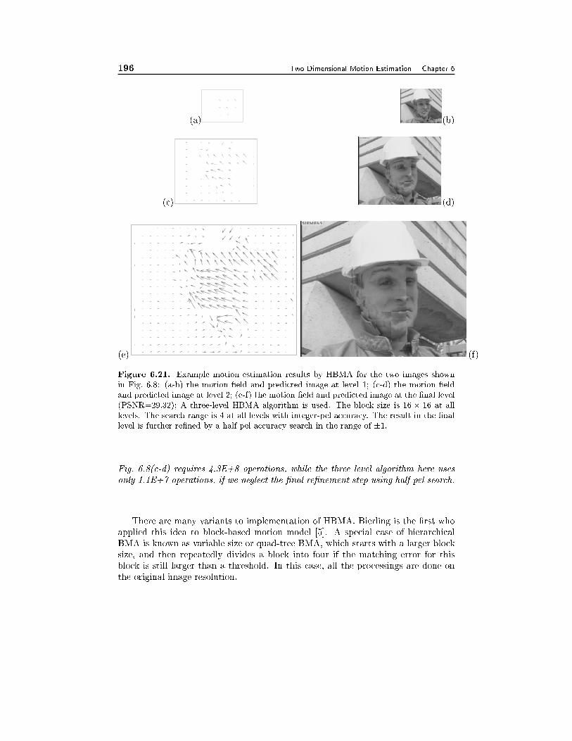
196 Two Dimensional Motion Estimation Chapter 6
(a) (b)
(c) (d)
(e) (f)
Figure 6.21. Example motion estimation results by HBMA for the two images shown
in Fig. 6.8: (a-b) the motion �eld and predicted image at level 1; (c-d) the motion �eld
and predicted image at level 2; (e-f) the motion �eld and predicted image at the �nal level
(PSNR=29.32); A three-level HBMA algorithm is used. The block size is 16 � 16 at all
levels. The search range is 4 at all levels with integer-pel accuracy. The result in the �nal
level is further re�ned by a half-pel accuracy search in the range of �1.
Fig. 6.8(c-d) requires 4.3E+8 operations, while the three level algorithm here uses
only 1.1E+7 operations, if we neglect the �nal re�nement step using half-pel search.
There are many variants to implementation of HBMA. Bierling is the �rst who
applied this idea to block-based motion model [5]. A special case of hierarchical
BMA is known as variable size or quad-tree BMA, which starts with a larger block
size, and then repeatedly divides a block into four if the matching error for this
block is still larger than a threshold. In this case, all the processings are done on
the original image resolution.
Section 6.10. Summary 197
6.10 Summary
Relation between Image Intensity and Motion
Almost all motion estimation algorithms are based on the constant intensity as-
sumption (Eq. (6.1.1) or Eq. (5.2.11)), or the optical ow equation (Eq. (6.1.3))
derived based on this assumption. This enables us to estimate motion by identi-
fying pixels with similar intensity, subject to some motion models. Note that this
assumption is valid only when the illumination source is ambient and temporally
invariant, and that the object surface is di�usely re ecting (Sec. 5.2).
When the motion direction is orthogonal to image intensity gradient, or if the
image gradient is zero, motion does not induce changes in image intensity. This is
the inherent limit of intensity based motion estimation methods.
Key Components in Motion Estimation
Motion representation: This depends on the partition used to divide a frame
(pixel-based, block-based, mesh-based, region-based, global), the motion model used
for each region of the partition (block, mesh-element, object-region, or entire frame),
and the constraint between motions in adjacent regions.
Motion estimation criterion: We presented three criteria for estimating the mo-
tion parameters over each region: i) minimizing DFD (when the motion is small,
this is equivalent to the method based on the optical- ow equation); ii) making the
resulting motion �eld as smooth as possible across regions, while minimizing DFD;
and iii) maximizing the a posterior probability of the motion �eld given the observed
frames. We showed that iii) essentially requires i) and ii). Instead of minimizing
DFD, one can also detect peaks in the PCF, when the motion in a region is a pure
translation.
Optimization methods: For chosen representation and criterion, the motion esti-
mation problem is usually converted to an optimization (minimization or maximiza-
tion) problem, which can be accomplished by using exhaustive search or gradient-
based search. To speech up the search and avoid being trapped in local minima, a
multi-resolution procedure can be used.
Application of Motion Estimation in Video Coding
Motion estimation is a key element in any video coding system. As will be discussed
in Sec. 9.3.1, an e�ective video coding method is to use block-wise temporal predic-
tion, by which a block in a frame to be coded is predicted from its corresponding
block in a previously coded frame, then the prediction error is coded. To minimize
the bit rate for coding the prediction error, the appropriate criterion for motion
estimation is to minimize the prediction error. The fact that the estimated motion
�eld does not necessarily resemble the actual motion �eld is not problematic in such
applications. Therefore, block matching algorithms described in Sec. 6.4 (EBMA
and its fast variant including HBMA) o�er simple and e�ective solutions. Instead of

198 Two Dimensional Motion Estimation Chapter 6
using the MV estimated for each block directly for the prediction of that block, one
can use a weighted average of the predicted values based on the MV's estimated for
its neighboring blocks. This is known as overlapping block motion compensation,
which will be discussed in Sec. 9.3.2.
Note that in the above video coding method, the motion vectors also need to
be coded, in addition to the prediction error. Therefore, minimizing the prediction
error alone is not the best criterion to use. Since a smoother motion �eld requires
fewer bits to code, imposing smoothness in the estimated motion �eld, if done
properly, can help improve the overall coding eÆciency. More advanced motion
estimation algorithms therefore operate by minimizing the total bit rate used for
coding the MVs and the prediction errors. This subject is discussed further in
Sec. 9.3.3.
To overcome the blocking artifacts produced by block-based motion estimation
methods, high-order block-based (DBMA), mesh-based or a combination of block-
based, mesh-based, and/or DBMA can be applied. However, these more compli-
cated schemes usually do not lead to signi�cant gain in the coding eÆciency.
In more advanced video coding schemes (Chap 10), global motion estimation is
usually applied to the entire frame, prior to block-based motion estimation, to
compensate the e�ect of camera motion. Moreover, an entire frame is usually
segmented into several regions or objects, and the motion parameters for each region
or object are estimated using the global motion estimation method discussed here.
6.11 Problems
6.1 Describe the pros and cons of di�erent motion representation methods (pixel-
based, block-based, mesh-based, global).
6.2 Describe the pros and cons of the exhaustive search and gradient descent
methods. Also compare between �rst order and second order gradient descent
methods.
6.3 What are the main advantages of the multi-resolution estimation method,
compared to an approach using a single resolution? Are there any disadvan-
tages?
6.4 In Sec. 6.3.2, we derived the multipoint neighborhood method using the gra-
dient descent method. Can you �nd a closed form solution using the optical
ow equation? Under what condition, will your solution be valid?
6.5 In Sec. 6.4.1, we described an exhaustive search algorithm for determine block
MVs in the block-based motion representation. Can you �nd a closed form
solution using the optical ow equation? Under what condition, will your
solution be valid?
6.6 In Eq. (6.2.7), we showed that, if the motion �eld is a constant, one can use the
optical ow equation to set up a least squares problem, and obtain a closed-
Section 6.11. Problems 199
form solution. Suppose that the motion �eld is not a constant, but can be
modeled by a polynomial mapping. Can you �nd a closed-form solution for
the polynomial coeÆcients?
Hint: any polynomial mapping function can be represented as d(x; a) = [A(x)]a,
where a contains all the polynomial coeÆcients.
6.7 In Sec. 6.4.5, we said that when there are several patches in a range block
in �1(x) that undergo di�erent motions, there will be several peaks in the
PCF. Each peak corresponds to the motion of one patch. The location of the
peak indicates the MV of the patch, whereas the amplitude of the peak is
proportional to the size of the patch. Can you prove this statement at least
qualitatively? You can simplify your derivation by considering the 1-D case
only.
6.8 With EBMA, does the computational requirement depends on the block size?
6.9 In Sec. 6.9.2, we derived the number of operations required by HBMA, if the
search range at every level is R=2L�1. What would be the number if one uses
a search range of �1 pel in every level, except at the �rst level, where the
search range is set to R=2L�1? Is this parameter set-up appropriate?
6.10 Consider a CCIR601 format video, with Y-component frame size of 720�480.
Compare the required computation by an EBMA algorithm (integer-pel) with
block size 16 � 16 and that by a two-level HBMA algorithm. Assume the
maximum motion range is �32: You can compare the computation by the op-
eration number with each operation including one subtraction, one absolute
value computation, and one addition. You can make your own assumption
about the search range at di�erent levels with HBMA. For simplicity, ig-
nore the computations required for generating the pyramid and assume only
integer-pel search.
6.11 Repeat the above for a three-level HBMA algorithm.
6.12 Write a C or Matlab code for implementing EBMA with integer-pel accuracy.
Use a block size of 16 � 16. The program should allow the user to choose
the search range, so that you can compare the results obtained with di�erent
search ranges. Note that the proper search range depends on the extent of
the motion in your test images. Apply the program to two adjacent frames
of a video sequence. Your program should produce and plot the estimated
motion �eld, the predicted frame, the prediction error image. It should also
calculate the PSNR of the predicted frame compared to the original tracked
frame. With Matlab, you can plot the motion �eld using the function quiver.
6.13 Repeat the above exercise for EBMA with half-pel accuracy. Compare the
PSNR of the predicted image obtained using integer-pel and that using half-
pel accuracy estimation. Which method gives you more accurate prediction?
200 Two Dimensional Motion Estimation Chapter 6
Which requires more computation time?
6.14 You can obtain a dense (i.e., pixel-based) motion �eld from a block-based one
by spatial interpolation. Write a C or Matlab code that can interpolate the
motion �eld resulting from Prob. 6.12 by assuming the MV for each block
is actually the MV of the block center. Use bilinear interpolation. Using
the interpolated pel-wise motion �eld, you can again produce the predicted
image and the prediction error image. Compare the motion �eld, predicted
image, and prediction error image obtained in Probs. 6.12 and 6.13 with those
obtained here. Which method gives you more accurate prediction? Which
requires more computation time?
6.15 Implement the HBMA method in C or Matlab. You can choose to use either
two or three levels of resolution. You can use integer-pel search at all levels, but
re�ne your �nal result by half-pel accuracy search within a �1 neighborhood.Use a block size of 16� 16 at all levels. The search range should be chosen so
that the equivalent search range in the original resolution is �32. Compare theresults with that obtained in Probs. 6.12 and 6.13, in terms of both accuracy
and computation time.
6.16 In Sec. 6.7, we say that the �tting error in Eq. (6.7.2) is minimized with the
solution given in Eq. (6.7.3). Prove this result yourself.
6.17 Assume the motion between two frames can be modeled by a global aÆne
model. We want to estimate the aÆne parameters directly based on the DFD
criterion. Set up the optimization problem, and derive an iterative algorithm
for solving the optimization problem. You can use either the �rst order gra-
dient descent or the Newton-Ralphson method. Write a C or Matlab code for
implementing your algorithm. Apply to two video frames that are undergoing
predominantly camera motion (e.g., , the ower garden sequence). Compare
the resulting motion �eld and predicted frame with that obtained with EBMA.
6.18 Repeat Prob. 6.17, but uses an indirect method to derive the aÆne param-
eters from given block motion vectors. Derive the regression equation and
the closed-form solution. Write a C or Matlab code for implementing your
algorithm. You can use your previous code for integer-pel EBMA to generate
block MVs. Compare the result obtained with the direct method (Prob. 6.17).
6.12 Bibliography
[1] J. K. Aggarwal and N. Nandhahumar. On the computation of motion from
sequences of images - a review. Proceedings of The IEEE, 76:917{935, 1988.
[2] Y. Altunbasak and A. M. Tekalp. Closed-form connectivity-preserving solutions
for motion compensation using 2-d meshes. IEEE Trans. Image Process., 6:1255{
1269, Sept. 1997.
Section 6.12. Bibliography 201
[3] Y. Altunbasak and A. M. Tekalp. Occlusion-adaptive, content-based mesh de-
sign and forward tracking. IEEE Trans. Image Process., 6:1270{1280, Sept. 1997.
[4] J. L. Barron, D. J. Fleet, and S. S. Beauchemin. Performance of optical ow
techniques. International Journal of Computer Vision, 12:43{77, 1994.
[5] M. Bierling. Displacement estimation by hierarchical block matching. In Proc.
SPIE: Visual Commun. Image Processing, volume SPIE-1001, pages 942{951,
Cambridge, MA, Nov. 1988.
[6] P. J. Burt and E. H. Adelson. The laplacian pyramid as a compact image code.
IEEE Trans. Commun., COM-31:532{540, 1983.
[7] P. Chou and C. Brown. The theory and practice of bayesian image labeling.
International Journal of Computer Vision, 4:185{210, 1990.
[8] R. O. Duda and P. E. Hart. Patterns classi�cation and Scene analysis. John
Wiley & Sons, 1973.
[9] D. J. Fleet and A. D. Jepson. Computation of component image velocity from
local phase information. International Journal of Computer Vision, 5:77{104,
1990.
[10] D.J. Fleet. Disparity from local weighted phase-correlation. In IEEE Interna-
tional Conference on Systems, Man, and Cybernetics: Humans, Information and
Technology, pages 48 {54, 1994.
[11] S. Geman and D. Geman. Stochastic relaxation, gibbs distributions, and the
baysian restoration of images. IEEE Trans. Pattern Anal. Machine Intell., 6:721{
741, Nov. 1984.
[12] B. Girod. Motion-compensating prediction with fractional-pel accuracy. IEEE
Trans. Commun., 41:604{612, 1993.
[13] B. Girod. Motion-compensating prediction with fractional-pel accuracy. IEEE
Transactions on Communications, 41(4):604{612, April 1993. -.
[14] H.-M. Hang, Y.-M. Chou, and S.-Chih. Cheng. Motion estimation for video
coding standards. Journal of VLSI Signal Processing Systems for Signal, Image,
and Video Technology, 17(2/3):113{136, Nov. 1997.
[15] R. M. Haralick and J. S. Lee. The facet approach to optical ow. In Proc.
Image Understanding Workshop, 1993.
[16] B. K. Horn and B. G. Schunck. Determining optical ow. Arti�cial intelligence,
17, 1981.
[17] B. K. P. Horn. Robot Vision. MIT Press, Cambridge, MA, 1986.
202 Two Dimensional Motion Estimation Chapter 6
[18] S. Hsu, P. Anandan, and S. Peleg. Accurate computation of optical ow using
layered motion rpresentations. In Proc. Int. Conf. Patt. Recog., pages 743{746,
Jerusalem, Israel, Oct. 1994.
[19] J. R. Jain and A. K. Jain. Displacement measurement and its application in
interframe image coding. IEEE Trans. Commun., COM-29:1799{1808, Dec. 1981.
[20] T. Koga et al. Motion-compensated interframe coding for video conferencing.
In Proc. Nat. Telecommun. Conf., pages G5.3.1{G5.3.5, New Orleans, LA, Nov.
1981.
[21] T. Komarek and P. Pirsch. Array architecture for block matching algorithms.
IEEE Trans. Circuits and Systems, 36:269{277, Oct. 1989.
[22] J. Konrad and E. Dubois. Baysian estimation of motion vector �elds. IEEE
Trans. Pattern Anal. Machine Intell., 14:910{927, Sept. 1992.
[23] C. Kuglin and D. Hines. The phase correlation image alignment method. In
Proc. IEEE Int. Conf. Cybern. Soc., pages 163{165, 1975.
[24] O. Lee and Y. Wang. Motion compensated prediction using nodal based de-
formable block matching. Journal of Visual Communications and Image Repre-
sentation, 6:26{34, Mar. 1995.
[25] X. Lee and Y.-Q. Zhang. A fast hierarchical motion compensation scheme for
video coding using block feature matching. IEEE Trans. Circuits Syst. for Video
Technology, 6:627{635, Dec. 1996.
[26] A. Mitchie, Y. F. Wang, and J. K. Aggarwal. Experiments in computing optical
ow with gradient-based multiconstraint methods. Pattern Recognition, 16, June
1983.
[27] H. G. Musmann, M. Hotter, and J. Ostermann. Object oriented analysis-
synthesis coding of moving images. Signal Processing: Image Commun., 1:119{138,
Oct. 1989.
[28] H.G. Musmann, P. Pirsch, and H.-J. Grallert. Advances in picture coding.
Proceedings of IEEE, 73(4):523{548, Apr. 1985.
[29] H. H. Nagel. Displacement vectors derived from second-order intensity varia-
tions in images sequences. Computer Graphics and Image Processing, 21:85{117,
1983.
[30] H. H. Nagel and W. Enklemann. An investigation of smoothness constraints for
the estimation of displacement vector �elds from image sequences. IEEE Trans.
Pattern Anal. Machine Intell., 8:565{593, Sept. 1986.
[31] A. N. Netravali and J. D. Robbins. Motion compensated coding: some new
results. Bell System Technical Journal, Nov. 1980.
Section 6.12. Bibliography 203
[32] P. Pirsch, N. Demassieux, and W. Gehrke. Vlsi architecture for video compres-
sion - a survey. Proc. IEEE, 83:220{246, Feb. 1995.
[33] B.S. Reddy and B.N. Chatterji. An �t-based technique for translation, rotation,
and scale-invariant image registration. IEEE Transactions on Image Processing,
5(8):1266{71, August 1996.
[34] J. Rissanen. A universal prior for intergers and estimation by minimum de-
scription length. The Annuals of Statistics, 11(2):416{431, 1983.
[35] P.J. Rousseeuw and A.M. Leroy. Robust Regression and Outlier Detection.
John Wiley & Sons, New York, 1987.
[36] V. Seferidis and M. Ghanbari. General approach to block matching motion
estimation. Optical Engineering, 32:1464{1474, July 1993.
[37] H. Shekarforoush, M. Berthod, and J. Zerubia. Subpixel image registration
by estimating the polyphase decomposition of cross power spectrum. In Proceed-
ings of the IEEE Computer Society Conference on Computer Vision and Pattern
Recognition 1996. IEEE, Los Alamitos, CA, pages 532{537, 1996.
[38] C. Stiller and J. Konrad. Estimating motion in image sequences. IEEE Signal
Processing Magazine, 16:70{91, July 1999.
[39] A. M. Tekalp. Digital Video Processing. Prentice Hall PTR, Upper Saddle
River, NJ, 1995.
[40] G. A. Thomas. Television motion measurements for datv and other applica-
tions. Research report 1987/11, BBC, September 1987.
[41] Y. Wang and O. Lee. Use of 2d deformable mesh structures for video com-
pression. part i | the synthesis problem: Mesh based function approximation and
mapping. IEEE Trans. Circuits Syst. for Video Technology, 6:636{646, Dec. 1996.
[42] Y. Wang and O. Lee. Active mesh | a feature seeking and tracking image
sequence representation scheme. IEEE Trans. Image Process., 3:610{624, Sept.
1994.
[43] Y. Wang and J. Ostermann. Evaluation of mesh-based motion estimation in
h.263 like coders. IEEE Trans. Circuits Syst. for Video Technology, 8:243{252,
June 1998.
[44] Y.Wang, X.-M. Hsieh, J.-H. Hu, and O.Lee. Region segmentation based on
active mesh representation of motion: comparison of parallel and sequential ap-
proaches. In Proc. Second IEEE International Conference on Image Processing
(ICIP'95), pages 185{188, Washington DC, Oct. 1995.
[45] O. C. Zienkewicz and R. L. Taylor. The �nite element method, volume 1.
Prentice Hall, 4th edition, 1989.
Chapter 7
THREE DIMENSIONAL
MOTION ESTIMATION
3D motion estimation allows for describing the motion of an object in 3D space.
The motion is estimated from images of the moving objects. It is used in computer
vision applications for object tracking as in vehicle guidance and robotics as well
as in object-based video coding for object tracking and motion compensation. In
some applications, a moving camera moves through a static scene, in others, a static
camera observes moving objects, and for some applications such as surveillance from
an airplane, the camera and objects move.
Similar to 2D motion estimation, 3D motion estimation is an ill-posed problem.
In order to ensure useful solutions, we make simplifying assumptions like rigid ob-
jects, usually of known shape. The task is to estimate the six motion parameters
of an object given in Eq. (5.3.9). Most algorithms assume that the object shape is
planar or parabolic, if the shape of an object is not known.
Both orthographic projection and perspective projections can be used as camera
models for 3D motion estimation. Naturally, the use of orthographic projection
simpli�es the estimation process. However, orthographic projection does not allow
us to observe depth and causes estimation errors if the object moves along the
optical axes of the camera or rotates around an axis other than the optical axis.
Another classi�cation of 3D motion estimation algorithms distinguishes between
direct methods that use the image signal as their input and indirect methods that
rely on feature correspondences that have been established with a separate algo-
rithm like block matching or feature matching. In section 7.1, we discuss algorithms
that estimate motion from feature correspondences. The precision of the estimated
motion parameters depends to a large extent on the precision of the feature corre-
spondences. Given these correspondences, the algorithms can easily estimate large
motion. Since motion is not estimated directly from the image signal but from
features derived from the image signal, we call these algorithms indirect motion
estimation methods. In section 7.2, we present direct motion estimation methods.
They have the advantage of not relying on feature correspondences. However, these
algorithms can only estimate small motion. Therefore, they are used in an iterative
204
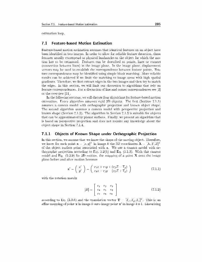
Section 7.1. Feature-based Motion Estimation 205
estimation loop.
7.1 Feature-based Motion Estimation
Feature-based motion estimation assumes that identical features on an object have
been identi�ed in two images. In order to allow for reliable feature detection, these
features usually correspond to physical landmarks on the object for which the mo-
tion has to be estimated. Features can be described as points, lines or corners
(connection between lines) in the image plane. In the image plane, displacement
vectors may be used to establish the correspondence between feature points. Fea-
ture correspondences may be identi�ed using simple block matching. More reliable
results can be achieved if we limit the matching to image areas with high spatial
gradients. Therefore, we �rst extract edges in the two images and then try to match
the edges. In this section, we will limit our discussion to algorithms that rely on
feature correspondences. For a discussion of line and corner correspondences see [2]
or the overview [11].
In the following sections, we will discuss four algorithms for feature-based motion
estimation. Every algorithm assumes rigid 3D objects. The �rst (Section 7.1.1)
assumes a camera model with orthographic projection and known object shape.
The second algorithm assumes a camera model with perspective projection and
known shape (Section 7.1.2). The algorithm in Section 7.1.3 is suitable for objects
that can be approximated by planar surfaces. Finally, we present an algorithm that
is based on perspective projection and does not require any knowledge about the
object shape in Section 7.1.4.
7.1.1 Objects of Known Shape under Orthographic Projection
In this section, we assume that we know the shape of the moving object. Therefore,
we know for each point x = [x; y]T in image k the 3D coordinates X = [X;Y; Z]T
of the object surface point associated with x. We use a camera model with or-
thographic projection according to Fig. 5.2(b) and Eq. (5.1.3). With this camera
model and Eq. (5.3.9) for 3D motion, the mapping of a point X onto the image
plane before and after motion becomes
x0 =
�x0
y0
�=
�r1x+ r2y + (r3Z + Tx)
r4x+ r5y + (r6Z + Ty)
�(7.1.1)
with the rotation matrix
[R] =
24 r1 r2 r3
r4 r5 r6
r7 r8 r9
35 (7.1.2)
according to Eq. (5.3.6) and the translation vector T = [Tx; Ty; Tz]T . This is an
aÆne mapping of point x in image k onto image point x0 in image k+1. Linearizing
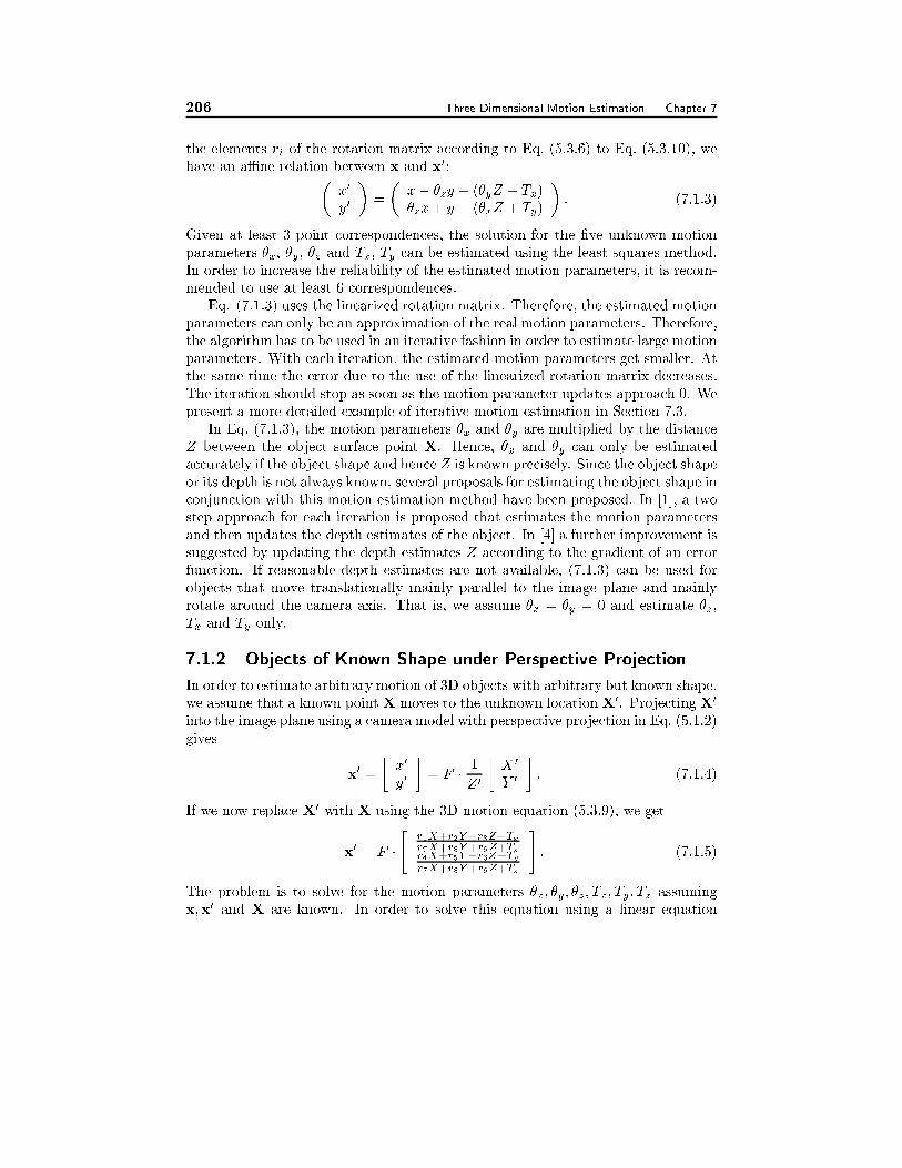
206 Three Dimensional Motion Estimation Chapter 7
the elements ri of the rotation matrix according to Eq. (5.3.6) to Eq. (5.3.10), we
have an aÆne relation between x and x0:�x0
y0
�=
�x� �zy + (�yZ + Tx)
�zx+ y � (�xZ + Ty)
�: (7.1.3)
Given at least 3 point correspondences, the solution for the �ve unknown motion
parameters �x, �y, �z and Tx, Ty can be estimated using the least squares method.
In order to increase the reliability of the estimated motion parameters, it is recom-
mended to use at least 6 correspondences.
Eq. (7.1.3) uses the linearized rotation matrix. Therefore, the estimated motion
parameters can only be an approximation of the real motion parameters. Therefore,
the algorithm has to be used in an iterative fashion in order to estimate large motion
parameters. With each iteration, the estimated motion parameters get smaller. At
the same time the error due to the use of the linearized rotation matrix decreases.
The iteration should stop as soon as the motion parameter updates approach 0. We
present a more detailed example of iterative motion estimation in Section 7.3.
In Eq. (7.1.3), the motion parameters �x and �y are multiplied by the distance
Z between the object surface point X. Hence, �x and �y can only be estimated
accurately if the object shape and hence Z is known precisely. Since the object shape
or its depth is not always known, several proposals for estimating the object shape in
conjunction with this motion estimation method have been proposed. In [1], a two
step approach for each iteration is proposed that estimates the motion parameters
and then updates the depth estimates of the object. In [4] a further improvement is
suggested by updating the depth estimates Z according to the gradient of an error
function. If reasonable depth estimates are not available, (7.1.3) can be used for
objects that move translationally mainly parallel to the image plane and mainly
rotate around the camera axis. That is, we assume �x = �y = 0 and estimate �z,
Tx and Ty only.
7.1.2 Objects of Known Shape under Perspective Projection
In order to estimate arbitrary motion of 3D objects with arbitrary but known shape,
we assume that a known point X moves to the unknown location X0. Projecting X0
into the image plane using a camera model with perspective projection in Eq. (5.1.2)
gives
x0 =
�x0
y0
�= F �
1
Z 0
�X
0
Y0
�: (7.1.4)
If we now replace X0 with X using the 3D motion equation (5.3.9), we get
x0 = F �
"r1X+r2Y+r3Z+Txr7X+r8Y+r9Z+Tzr4X+r5Y+r6Z+Tyr7X+r8Y+r9Z+Tz
#: (7.1.5)
The problem is to solve for the motion parameters �x; �y; �z; Tx; Ty; Tz assuming
x;x0 and X are known. In order to solve this equation using a linear equation
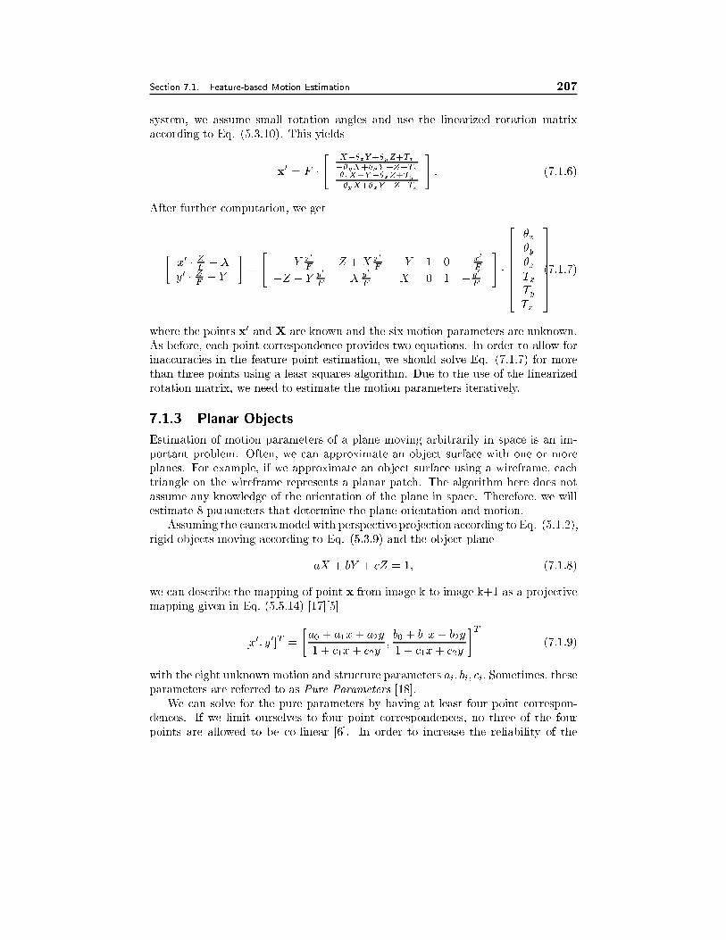
Section 7.1. Feature-based Motion Estimation 207
system, we assume small rotation angles and use the linearized rotation matrix
according to Eq. (5.3.10). This yields
x0 = F �
"X��zY+�yZ+Tx��yX+�xY+Z+Tz�zX+Y��xZ+Ty��yX+�xY+Z+Tz
#: (7.1.6)
After further computation, we get
�x0�ZF�X
y0�ZF� Y
�=
"�Y
x0
FZ +X
x0
F�Y 1 0 �
x0
F
�Z � Yy0
FXy0
FX 0 1 �
y0
F
#�
26666664
�x
�y
�z
Tx
Ty
Tz
37777775(7.1.7)
where the points x0 and X are known and the six motion parameters are unknown.
As before, each point correspondence provides two equations. In order to allow for
inaccuracies in the feature point estimation, we should solve Eq. (7.1.7) for more
than three points using a least squares algorithm. Due to the use of the linearized
rotation matrix, we need to estimate the motion parameters iteratively.
7.1.3 Planar Objects
Estimation of motion parameters of a plane moving arbitrarily in space is an im-
portant problem. Often, we can approximate an object surface with one or more
planes. For example, if we approximate an object surface using a wireframe, each
triangle on the wireframe represents a planar patch. The algorithm here does not
assume any knowledge of the orientation of the plane in space. Therefore, we will
estimate 8 parameters that determine the plane orientation and motion.
Assuming the cameramodel with perspective projection according to Eq. (5.1.2),
rigid objects moving according to Eq. (5.3.9) and the object plane
aX + bY + cZ = 1; (7.1.8)
we can describe the mapping of point x from image k to image k+1 as a projective
mapping given in Eq. (5.5.14) [17][5]
[x0; y0]T =
�a0 + a1x+ a2y
1 + c1x+ c2y;b0 + b1x+ b2y
1 + c1x+ c2y
�T(7.1.9)
with the eight unknown motion and structure parameters ai; bi; ci: Sometimes, these
parameters are referred to as Pure Parameters [18].
We can solve for the pure parameters by having at least four point correspon-
dences. If we limit ourselves to four point correspondences, no three of the four
points are allowed to be co-linear [6]. In order to increase the reliability of the
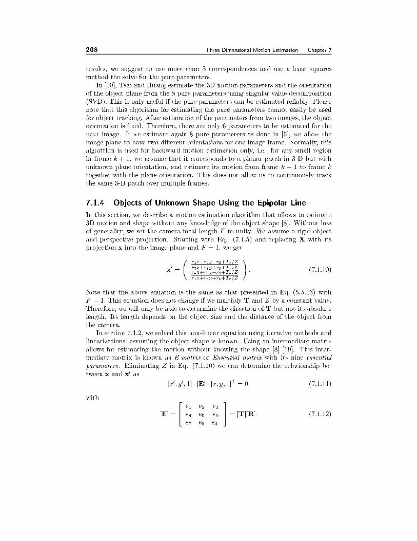
208 Three Dimensional Motion Estimation Chapter 7
results, we suggest to use more than 8 correspondences and use a least squares
method the solve for the pure parameters.
In [20], Tsai and Huang estimate the 3D motion parameters and the orientation
of the object plane from the 8 pure parameters using singular value decomposition
(SVD). This is only useful if the pure parameters can be estimated reliably. Please
note that this algorithm for estimating the pure parameters cannot easily be used
for object tracking. After estimation of the parameters from two images, the object
orientation is �xed. Therefore, there are only 6 parameters to be estimated for the
next image. If we estimate again 8 pure parameters as done in [5], we allow the
image plane to have two di�erent orientations for one image frame. Normally, this
algorithm is used for backward motion estimation only, i.e., for any small region
in frame k + 1, we assume that it corresponds to a planar patch in 3-D but with
unknown plane orientation, and estimate its motion from frame k + 1 to frame k
together with the plane orientation. This does not allow us to continuously track
the same 3-D patch over multiple frames.
7.1.4 Objects of Unknown Shape Using the Epipolar Line
In this section, we describe a motion estimation algorithm that allows to estimate
3D motion and shape without any knowledge of the object shape [8]. Without loss
of generality, we set the camera focal length F to unity. We assume a rigid object
and perspective projection. Starting with Eq. (7.1.5) and replacing X with its
projection x into the image plane and F = 1, we get
x0 =
r1x+r2y+r3+Tx=Z
r7x+r8y+r9+Tz=Zr4x+r5y+r6+Ty=Z
r7x+r8y+r9+Tz=Z
!: (7.1.10)
Note that the above equation is the same as that presented in Eq. (5.5.13) with
F = 1: This equation does not change if we multiply T and Z by a constant value.
Therefore, we will only be able to determine the direction of T but not its absolute
length. Its length depends on the object size and the distance of the object from
the camera.
In section 7.1.2, we solved this non-linear equation using iterative methods and
linearizations, assuming the object shape is known. Using an intermediate matrix
allows for estimating the motion without knowing the shape [8] [19]. This inter-
mediate matrix is known as E-matrix or Essential matrix with its nine essential
parameters. Eliminating Z in Eq. (7.1.10) we can determine the relationship be-
tween x and x0 as
[x0; y0; 1] � [E] � [x; y; 1]T = 0; (7.1.11)
with
[E] =
24 e1 e2 e3
e4 e5 e6
e7 e8 e9
35 = [T][R]: (7.1.12)
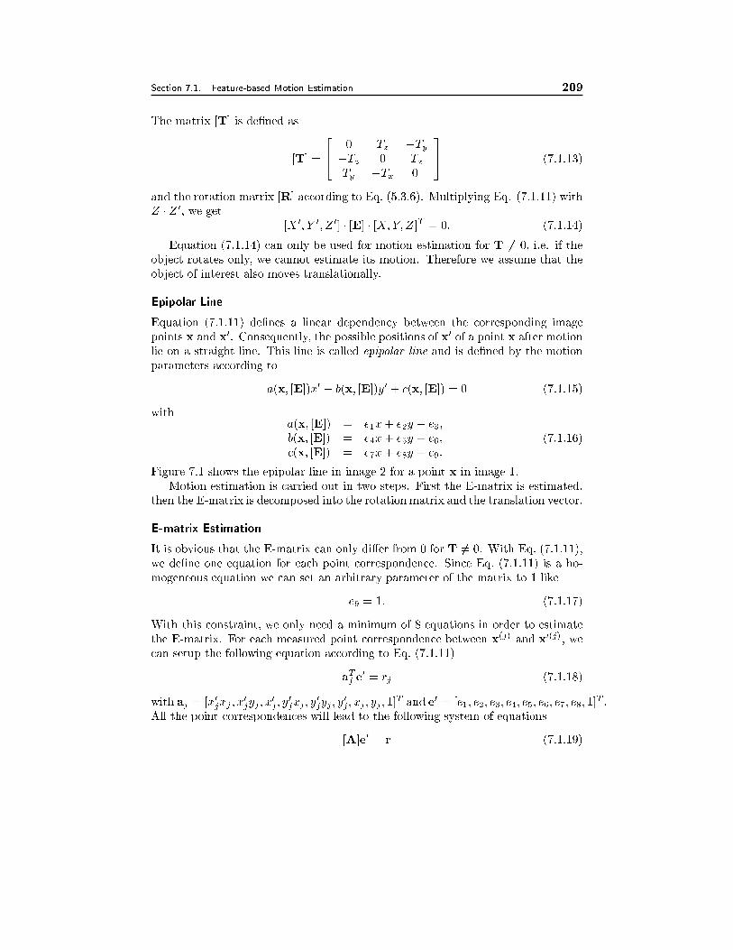
Section 7.1. Feature-based Motion Estimation 209
The matrix [T] is de�ned as
[T] =
24 0 Tz �Ty
�Tz 0 Tx
Ty �Tx 0
35 (7.1.13)
and the rotation matrix [R] according to Eq. (5.3.6). Multiplying Eq. (7.1.11) with
Z � Z0, we get
[X 0; Y
0; Z
0] � [E] � [X;Y; Z]T = 0: (7.1.14)
Equation (7.1.14) can only be used for motion estimation for T 6= 0, i.e. if the
object rotates only, we cannot estimate its motion. Therefore we assume that the
object of interest also moves translationally.
Epipolar Line
Equation (7.1.11) de�nes a linear dependency between the corresponding image
points x and x0. Consequently, the possible positions of x0 of a point x after motion
lie on a straight line. This line is called epipolar line and is de�ned by the motion
parameters according to
a(x; [E])x0 + b(x; [E])y0 + c(x; [E]) = 0 (7.1.15)
witha(x; [E]) = e1x+ e2y + e3;
b(x; [E]) = e4x+ e5y + e6;
c(x; [E]) = e7x+ e8y + e9:
(7.1.16)
Figure 7.1 shows the epipolar line in image 2 for a point x in image 1.
Motion estimation is carried out in two steps. First the E-matrix is estimated,
then the E-matrix is decomposed into the rotation matrix and the translation vector.
E-matrix Estimation
It is obvious that the E-matrix can only di�er from 0 for T 6= 0. With Eq. (7.1.11),
we de�ne one equation for each point correspondence. Since Eq. (7.1.11) is a ho-
mogeneous equation we can set an arbitrary parameter of the matrix to 1 like
e9 = 1: (7.1.17)
With this constraint, we only need a minimum of 8 equations in order to estimate
the E-matrix. For each measured point correspondence between x(j) and x0(j), we
can setup the following equation according to Eq. (7.1.11)
aTj e0 = rj (7.1.18)
with aj = [x0jxj ; x0
jyj ; x0
j ; y0
jxj ; y0
jyj ; y0
j ; xj ; yj ; 1]T and e0 = [e1; e2; e3; e4; e5; e6; e7; e8; 1]
T .
All the point correspondences will lead to the following system of equations
[A]e0 = r (7.1.19)
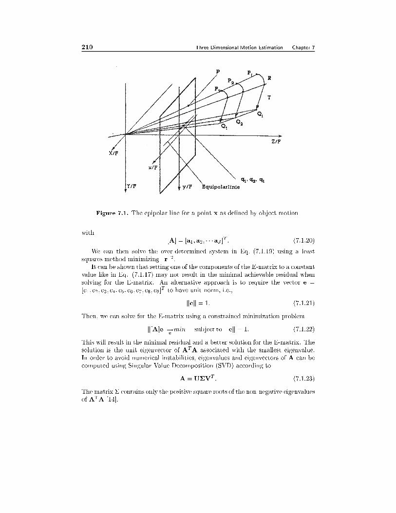
210 Three Dimensional Motion Estimation Chapter 7
Figure 7.1. The epipolar line for a point x as de�ned by object motion
with
[A] = [a1; a2; � � �aJ ]T: (7.1.20)
We can then solve the over-determined system in Eq. (7.1.19) using a least
squares method minimizing krk2.
It can be shown that setting one of the components of the E-matrix to a constant
value like in Eq. (7.1.17) may not result in the minimal achievable residual when
solving for the E-matrix. An alternative approach is to require the vector e =
[e1; e2; e3; e4; e5; e6; e7; e8; e9]T to have unit norm, i.e.,
kek = 1: (7.1.21)
Then, we can solve for the E-matrix using a constrained minimization problem
k[A]ek�!emin subject to kek = 1: (7.1.22)
This will result in the minimal residual and a better solution for the E-matrix. The
solution is the unit eigenvector of ATA associated with the smallest eigenvalue.
In order to avoid numerical instabilities, eigenvalues and eigenvectors of A can be
computed using Singular Value Decomposition (SVD) according to
A = U�VT: (7.1.23)
The matrix � contains only the positive square roots of the non-negative eigenvalues
of ATA [14].
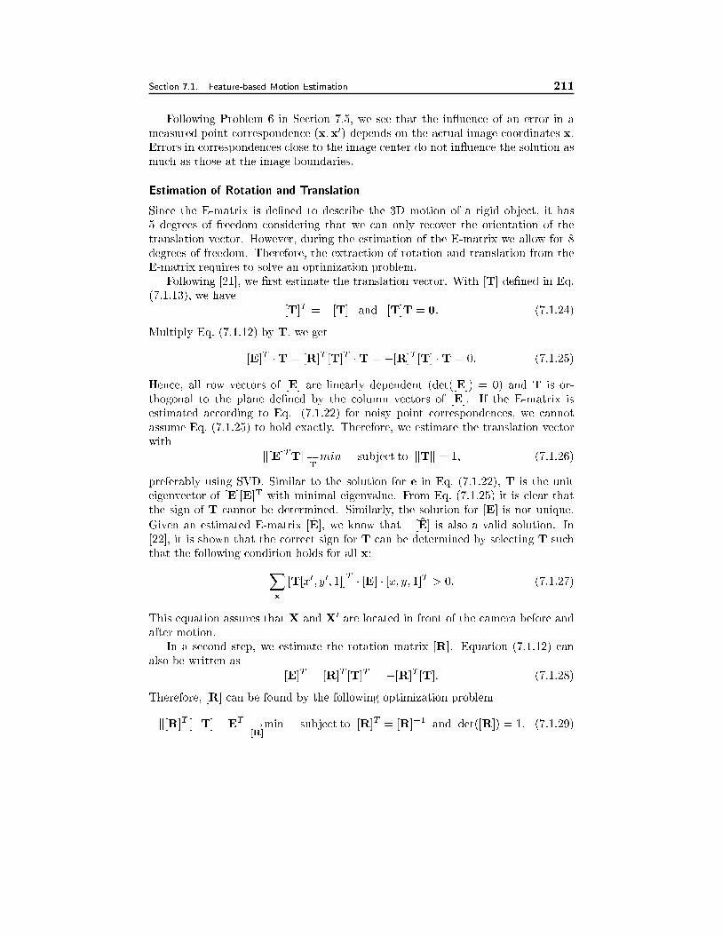
Section 7.1. Feature-based Motion Estimation 211
Following Problem 6 in Section 7.5, we see that the in uence of an error in a
measured point correspondence (x;x0) depends on the actual image coordinates x.
Errors in correspondences close to the image center do not in uence the solution as
much as those at the image boundaries.
Estimation of Rotation and Translation
Since the E-matrix is de�ned to describe the 3D motion of a rigid object, it has
5 degrees of freedom considering that we can only recover the orientation of the
translation vector. However, during the estimation of the E-matrix we allow for 8
degrees of freedom. Therefore, the extraction of rotation and translation from the
E-matrix requires to solve an optimization problem.
Following [21], we �rst estimate the translation vector. With [T] de�ned in Eq.
(7.1.13), we have
[T]T = �[T] and [T]T = 0: (7.1.24)
Multiply Eq. (7.1.12) by T, we get
[E]T �T = [R]T [T]T �T = �[R]T [T] �T = 0: (7.1.25)
Hence, all row vectors of [E] are linearly dependent (det([E]) = 0) and T is or-
thogonal to the plane de�ned by the column vectors of [E]. If the E-matrix is
estimated according to Eq. (7.1.22) for noisy point correspondences, we cannot
assume Eq. (7.1.25) to hold exactly. Therefore, we estimate the translation vector
with
k[E]TTk�!T
min subject to kTk = 1; (7.1.26)
preferably using SVD. Similar to the solution for e in Eq. (7.1.22), T is the unit
eigenvector of [E][E]T with minimal eigenvalue. From Eq. (7.1.25) it is clear that
the sign of T cannot be determined. Similarly, the solution for [E] is not unique.
Given an estimated E-matrix [E], we know that �[E] is also a valid solution. In
[22], it is shown that the correct sign for T can be determined by selecting T such
that the following condition holds for all x:Xx
[T[x0; y0; 1]]T� [E] � [x; y; 1]T > 0: (7.1.27)
This equation assures that X and X0 are located in front of the camera before and
after motion.
In a second step, we estimate the rotation matrix [R]. Equation (7.1.12) can
also be written as
[E]T = [R]T [T]T = �[R]T [T]: (7.1.28)
Therefore, [R] can be found by the following optimization problem
k[R]T [�T]�ET k�![R]
min subject to [R]T = [R]�1 and det([R]) = 1: (7.1.29)
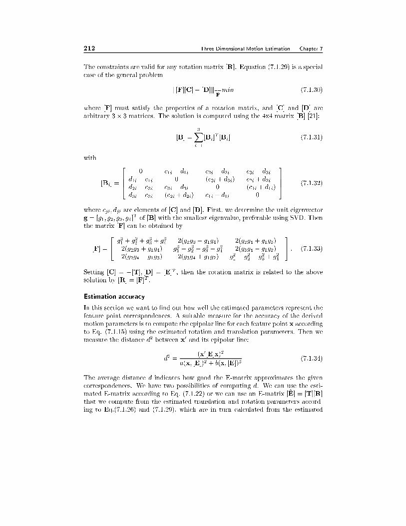
212 Three Dimensional Motion Estimation Chapter 7
The constraints are valid for any rotation matrix [R]. Equation (7.1.29) is a special
case of the general problem
k[F][C]� [D]k�![F]min (7.1.30)
where [F] must satisfy the properties of a rotation matrix, and [C] and [D] are
arbitrary 3� 3 matrices. The solution is computed using the 4x4 matrix [B] [21]:
[B] =
3Xi=1
[Bi]T [Bi] (7.1.31)
with
[Bi] =
2664
0 c1i � d1i c2i � d2i c3i � d3i
d1i � c1i 0 �(c3i + d3i) c2i + d2i
d2i � c3i c3i + d3i 0 �(c1i + d1i)
d3i � c3i �(c2i + d2i) c1i + d1i 0
3775 (7.1.32)
where cji; dji are elements of [C] and [D]. First, we determine the unit eigenvector
g = [g1; g2; g3; g4]T of [B] with the smallest eigenvalue, preferable using SVD. Then
the matrix [F] can be obtained by
[F] =
24 g
21 + g
22 + g
23 + g
24 2(g2g3 � g1g4) 2(g2g4 + g1g3)
2(g2g3 + g1g4) g21 � g
22 + g
23 � g
24 2(g3g4 � g1g2)
2(g2g4 � g1g3) 2(g3g4 + g1g2) g21 � g
22 � g
23 + g
24
35 : (7.1.33)
Setting [C] = �[T]; [D] = [E]T , then the rotation matrix is related to the above
solution by [R] = [F]T :
Estimation accuracy
In this section we want to �nd out how well the estimated parameters represent the
feature point correspondences. A suitable measure for the accuracy of the derived
motion parameters is to compute the epipolar line for each feature point x according
to Eq. (7.1.15) using the estimated rotation and translation parameters. Then we
measure the distance d2 between x0 and its epipolar line:
d2 =
(x0[E]x)2
a(x; [E])2 + b(x; [E])2(7.1.34)
The average distance �d indicates how good the E-matrix approximates the given
correspondences. We have two possibilities of computing �d. We can use the esti-
mated E-matrix according to Eq. (7.1.22) or we can use an E-matrix [E] = [T][R]
that we compute from the estimated translation and rotation parameters accord-
ing to Eq.(7.1.26) and (7.1.29), which are in turn calculated from the estimated
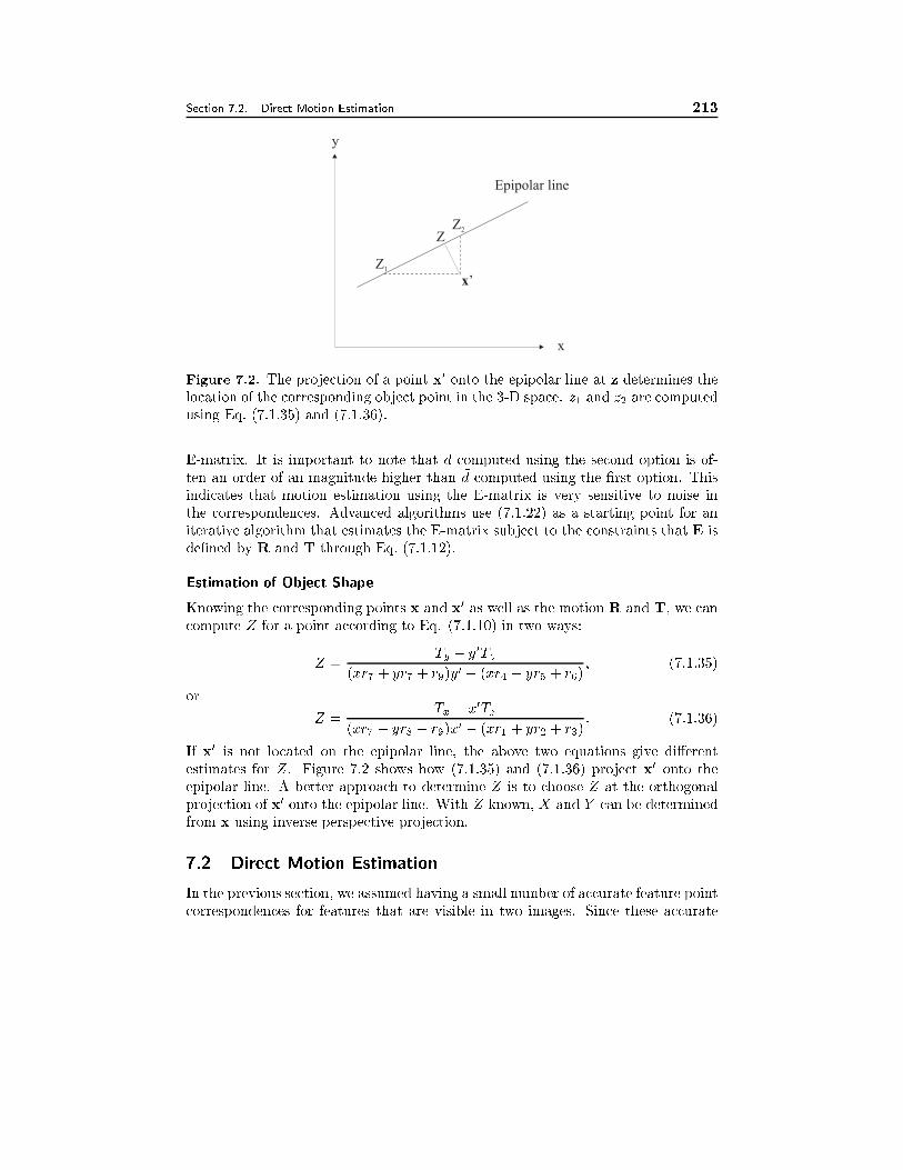
Section 7.2. Direct Motion Estimation 213
x
y
x’
Z2
Z1
Z
Epipolar line
Figure 7.2. The projection of a point x0 onto the epipolar line at z determines the
location of the corresponding object point in the 3-D space. z1 and z2 are computed
using Eq. (7.1.35) and (7.1.36).
E-matrix. It is important to note that �d computed using the second option is of-
ten an order of an magnitude higher than �d computed using the �rst option. This
indicates that motion estimation using the E-matrix is very sensitive to noise in
the correspondences. Advanced algorithms use (7.1.22) as a starting point for an
iterative algorithm that estimates the E-matrix subject to the constraints that E is
de�ned by R and T through Eq. (7.1.12).
Estimation of Object Shape
Knowing the corresponding points x and x0 as well as the motion R and T, we can
compute Z for a point according to Eq. (7.1.10) in two ways:
Z =Ty � y
0Tz
(xr7 + yr7 + r9)y0 � (xr4 + yr5 + r6); (7.1.35)
or
Z =Tx � x
0Tz
(xr7 + yr8 + r9)x0 � (xr1 + yr2 + r3): (7.1.36)
If x0 is not located on the epipolar line, the above two equations give di�erent
estimates for Z. Figure 7.2 shows how (7.1.35) and (7.1.36) project x0 onto the
epipolar line. A better approach to determine Z is to choose Z at the orthogonal
projection of x0 onto the epipolar line. With Z known, X and Y can be determined
from x using inverse perspective projection.
7.2 Direct Motion Estimation
In the previous section, we assumed having a small number of accurate feature point
correspondences for features that are visible in two images. Since these accurate
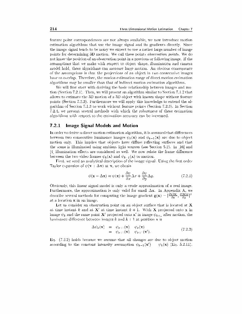
214 Three Dimensional Motion Estimation Chapter 7
feature point correspondences are not always available, we now introduce motion
estimation algorithms that use the image signal and its gradients directly. Since
the image signal tends to be noisy we expect to use a rather large number of image
points for determining 3D motion. We call these points observation points. We do
not know the position of an observation point in a previous or following image. If the
assumptions that we make with respect to object shape, illumination and camera
model hold, these algorithms can measure large motion. An obvious consequence
of the assumptions is that the projections of an object in two consecutive images
have to overlap. Therefore, the motion estimation range of direct motion estimation
algorithms may be smaller than that of indirect motion estimation algorithms.
We will �rst start with deriving the basic relationship between images and mo-
tion (Section 7.2.1). Then, we will present an algorithm similar to Section 7.1.2 that
allows to estimate the 3D motion of a 3D object with known shape without feature
points (Section 7.2.2). Furthermore we will apply this knowledge to extend the al-
gorithm of Section 7.1.3 to work without feature points (Section 7.2.3). In Section
7.2.4, we present several methods with which the robustness of these estimation
algorithms with respect to the estimation accuracy can be increased.
7.2.1 Image Signal Models and Motion
In order to derive a direct motion estimation algorithm, it is assumed that di�erences
between two consecutive luminance images k(x) and k+1(x) are due to object
motion only. This implies that objects have di�use re ecting surfaces and that
the scene is illuminated using ambient light sources (see Section 5.2). In [16] and
[4] illumination e�ects are considered as well. We now relate the frame di�erence
between the two video frames k(x) and k+1(x) to motion.
First, we need an analytical description of the image signal. Using the �rst order
Taylor expansion of (x+�x) at x, we obtain
(x+�x) � (x) +@
@x�x+
@
@y�y: (7.2.1)
Obviously, this linear signal model is only a crude approximation of a real image.
Furthermore, the approximation is only valid for small �x. In Appendix A, we
describe several methods for computing the image gradient g(x) = [@ (x)
@x;@(x)
@y]T
at a location x in an image.
Let us consider an observation point on an object surface that is located at X
at time instant k and at X0 at time instant k + 1. With X projected onto x in
image k and the same point X0 projected onto x0 in image k+1 after motion, the
luminance di�erence between images k and k + 1 at position x is
� k(x) = k+1(x)� k(x)
= k+1(x)� k+1(x0):
(7.2.2)
Eq. (7.2.2) holds because we assume that all changes are due to object motion
according to the constant intensity assumption k+1(x0) = k(x) (Eq. 5.2.11).
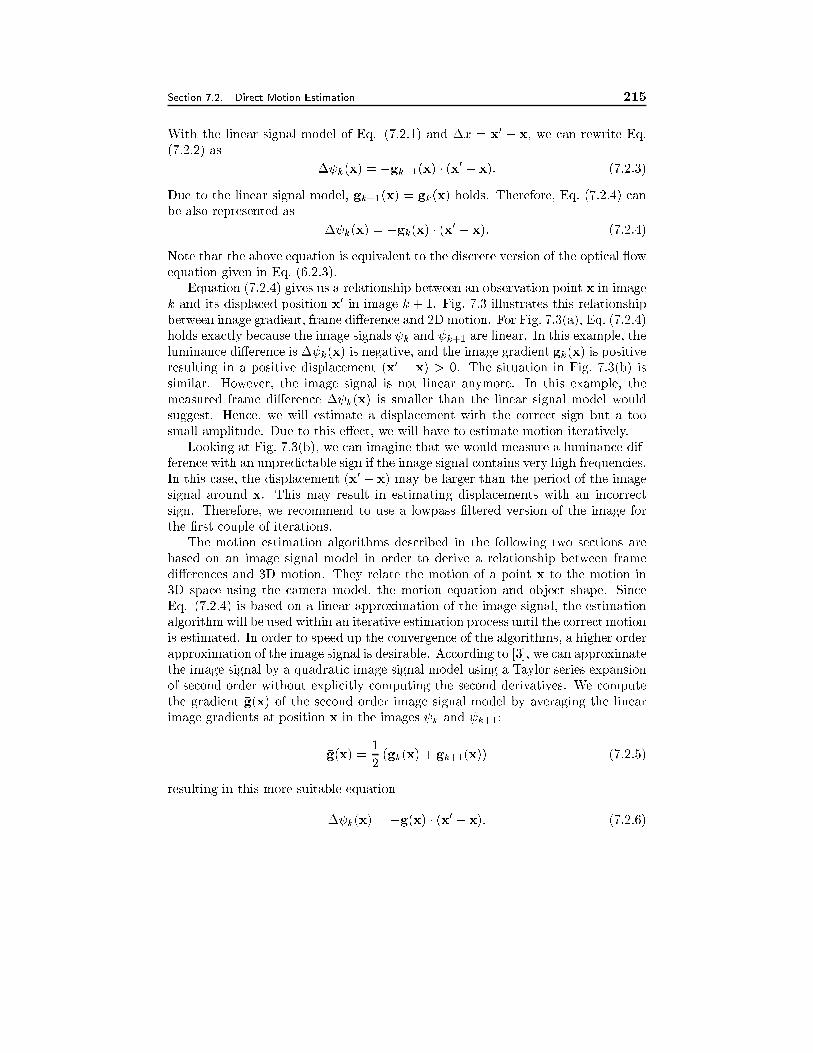
Section 7.2. Direct Motion Estimation 215
With the linear signal model of Eq. (7.2.1) and �x = x0 � x, we can rewrite Eq.
(7.2.2) as
� k(x) = �gk+1(x) � (x0� x): (7.2.3)
Due to the linear signal model, gk+1(x) = gk(x) holds. Therefore, Eq. (7.2.4) can
be also represented as
� k(x) = �gk(x) � (x0� x): (7.2.4)
Note that the above equation is equivalent to the discrete version of the optical ow
equation given in Eq. (6.2.3).
Equation (7.2.4) gives us a relationship between an observation point x in image
k and its displaced position x0 in image k + 1. Fig. 7.3 illustrates this relationship
between image gradient, frame di�erence and 2D motion. For Fig. 7.3(a), Eq. (7.2.4)
holds exactly because the image signals k and k+1 are linear. In this example, the
luminance di�erence is � k(x) is negative, and the image gradient gk(x) is positive
resulting in a positive displacement (x0 � x) > 0. The situation in Fig. 7.3(b) is
similar. However, the image signal is not linear anymore. In this example, the
measured frame di�erence � k(x) is smaller than the linear signal model would
suggest. Hence, we will estimate a displacement with the correct sign but a too
small amplitude. Due to this e�ect, we will have to estimate motion iteratively.
Looking at Fig. 7.3(b), we can imagine that we would measure a luminance dif-
ference with an unpredictable sign if the image signal contains very high frequencies.
In this case, the displacement (x0 � x) may be larger than the period of the image
signal around x. This may result in estimating displacements with an incorrect
sign. Therefore, we recommend to use a lowpass �ltered version of the image for
the �rst couple of iterations.
The motion estimation algorithms described in the following two sections are
based on an image signal model in order to derive a relationship between frame
di�erences and 3D motion. They relate the motion of a point x to the motion in
3D space using the camera model, the motion equation and object shape. Since
Eq. (7.2.4) is based on a linear approximation of the image signal, the estimation
algorithm will be used within an iterative estimation process until the correct motion
is estimated. In order to speed up the convergence of the algorithms, a higher order
approximation of the image signal is desirable. According to [3], we can approximate
the image signal by a quadratic image signal model using a Taylor series expansion
of second order without explicitly computing the second derivatives. We compute
the gradient �g(x) of the second order image signal model by averaging the linear
image gradients at position x in the images k and k+1:
�g(x) =1
2(gk(x) + gk+1(x)) (7.2.5)
resulting in this more suitable equation
� k(x) = ��g(x) � (x0 � x): (7.2.6)
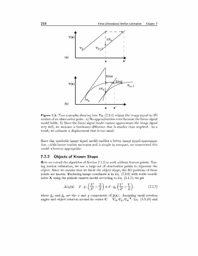
216 Three Dimensional Motion Estimation Chapter 7
���
������
x x’
�(x)
���
����
��
x x’
�(x)
Error
Error
(b)
�a)
Figure 7.3. Two examples showing how Eq. (7.2.4) relates the image signal to 2D
motion of an observation point. a) No approximation error because the linear signal
model holds. b) Since the linear signal model cannot approximate the image signal
very well, we measure a luminance di�erence that is smaller than required. As a
result, we estimate a displacement that is too small.
Since this quadratic image signal model enables a better image signal approxima-
tion, yields better motion estimates and is simple to compute, we recommend this
model whenever appropriate.
7.2.2 Objects of Known Shape
Here we extend the algorithm of Section 7.1.2 to work without feature points. Dur-
ing motion estimation, we use a large set of observation points to represent the
object. Since we assume that we know the object shape, the 3D positions of these
points are known. Replacing image coordinate x in Eq. (7.2.6) with world coordi-
nates X using the pinhole camera model according to Eq. (5.1.2), we get
� k(x) = F � �gx
�X
0
Z 0�
X
Z
�+ F � �gy
�Y0
Z 0�
Y
Z
�: (7.2.7)
where �gx and �gy are the x and y components of �g(x). Assuming small rotation
angles and object rotation around its center C = [Cx;Cy;Cz]T, Eq. (5.3.10) and
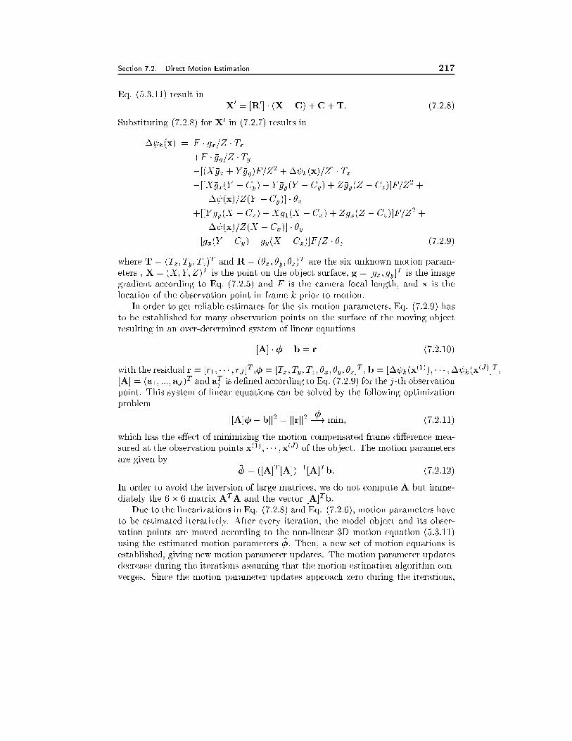
Section 7.2. Direct Motion Estimation 217
Eq. (5.3.11) result in
X0 = [R0] � (X�C) +C+T: (7.2.8)
Substituting (7.2.8) for X0 in (7.2.7) results in
� k(x) = F � �gx=Z � Tx
+F � �gy=Z � Ty
�[(X�gx + Y �gy)F=Z2 +� k(x)=Z] � Tz
�[[X�gx(Y � Cy) + Y �gy(Y � Cy) + Z�gy(Z � Cz)]F=Z2 +
� (x)=Z(Y � Cy)] � �x
+[[Y �gy(X � Cx) +X�g1(X � Cx) + Z�gx(Z � Cz)]F=Z2 +
� (x)=Z(X � Cx)] � �y
�[�gx(Y � Cy)� �gy(X � Cx)]F=Z � �z (7.2.9)
where T = (Tx; Ty; Tz)T and R = (�x; �y; �z)
T are the six unknown motion param-
eters , X = (X;Y; Z)T is the point on the object surface, �g = [�gx; �gy]T is the image
gradient according to Eq. (7.2.5) and F is the camera focal length, and x is the
location of the observation point in frame k prior to motion.
In order to get reliable estimates for the six motion parameters, Eq. (7.2.9) has
to be established for many observation points on the surface of the moving object
resulting in an over-determined system of linear equations
[A] � �� b = r (7.2.10)
with the residual r = [r1; � � � ; rJ ]T ,� = [Tx; Ty; Tz; �x; �y; �z]
T , b = [� k(x(1)); � � � ;� k(x
(J)]T ,
[A] = (a1; :::; aJ )T and aTj is de�ned according to Eq. (7.2.9) for the j-th observation
point. This system of linear equations can be solved by the following optimization
problem
k[A]�� bk2 = krk2��! min; (7.2.11)
which has the e�ect of minimizing the motion compensated frame di�erence mea-
sured at the observation points x(1); � � � ;x(J) of the object. The motion parameters
are given by
� = ([A]T [A])�1[A]Tb: (7.2.12)
In order to avoid the inversion of large matrices, we do not compute A but imme-
diately the 6� 6 matrix ATA and the vector [A]Tb.
Due to the linearizations in Eq. (7.2.8) and Eq. (7.2.6), motion parameters have
to be estimated iteratively. After every iteration, the model object and its obser-
vation points are moved according to the non-linear 3D motion equation (5.3.11)
using the estimated motion parameters �. Then, a new set of motion equations is
established, giving new motion parameter updates. The motion parameter updates
decrease during the iterations assuming that the motion estimation algorithm con-
verges. Since the motion parameter updates approach zero during the iterations,
218 Three Dimensional Motion Estimation Chapter 7
the error due to the linearization of the rotation matrix also approaches 0. The
iteration process terminates if the decrease of the residual kA� � bk2 becomes
negligible.
This algorithm estimates object motion from frame k to k + 1. Due to this
forward motion estimation, we can track an object as it is moving forward in a
video scene.
7.2.3 Planar Objects
Planar objects are often used as an approximation for real objects (Sec. 5.5.3). Since
these approximations are usually not used for tracking but for motion compensation
in video coding, we now extend the algorithm presented in Section 7.1.3 to a direct
estimation method [5] that estimates motion backward. Starting with Eq. (7.1.9)
de�ning the mapping A(x; y) of a point x in image k + 1 to x0 in image k with
x0 = (x0; y0)T
= [Ax(x); Ay(x)]T
=
�a1x+ a2y + a3
a7x+ a8y + 1;a4x+ a5y + a6
a7x+ a8y + 1
�T= A(x) (7.2.13)
and assuming again that all changes in the image sequence are due to object motion,
we get
k+1(x) = k(x0) = k(A(x)): (7.2.14)
The frame di�erence similar to Eq. (7.2.2) becomes
� k(x) = k+1(x) � k(x)
= k(A(x)) � k(x):(7.2.15)
With a Taylor series expansion we express the luminance function at an obser-
vation point x with respect to the motion parameters ai:
k(A(x)) =
k(xk) +
8Xi=1
@ k(x)
@ai�ai +
1
2
8Xi=1
8Xj=1
@ k(x)
@ai
@ k(x)
@aj�ai�aj +R2(x):(7.2.16)
Using this in Eq. (7.2.15), results in
� k(x) =
8Xi=1
@ k(x)
@ai�ai +
1
2
8Xi=1
8Xj=1
@ k(x)
@ai
@ k(x)
@aj�ai�aj +R2(x): (7.2.17)
with �a = a�e, e = (1; 0; 0; 0; 1; 0; 0; 0)T , a = (a1; � � � ; a8)T ,@ k(x)
@ai=
@ k(x)
@ai
@ k(x)
@x
and R2(x) denoting the higher order terms of the Taylor series expansion. If
Section 7.2. Direct Motion Estimation 219
the quadratic image signal model is valid, this residual R2(x) is zero simplifying
Eq. (7.2.17) to
� k(x) = �gxx�a1 + �gxy�a2 + �gx�a3 + �gyx�a4 + �gyy�a5
+�gy�a6 � x(�gxx+ �gyy)�a7 � y(�gxx+ �gyy)�a8
= hT�a: (7.2.18)
with@ k(x)
@ai=
@ k(x)
@x
@Ax(x)
@ai+
@ k(x)
@y
@Ay(x)
@aiand �g(x) = [�gx; �gy]
T according to
Eq. (7.2.6).
Eq. (7.2.18) de�nes an equation for one observation point of the object with
the 8 unknown motion parameters. In order to estimate the motion, we set up
Eq. (7.2.18) for J observation points x and solve the following system of J linear
equations
[H]�a = � : (7.2.19)
The row vectors of matrix [H] are the hT determined according to Eq. (7.2.18),
� is a vector with the frame di�erences between the two images according to
Eq. (7.2.18). Solving this system of linear equations with the least squares method,
we get, similar to (7.2.12),
�a = ([H]T [H])�1[H]T� : (7.2.20)
Due to the approximations used in the image signal model, this estimation process
has to be carried out iteratively. After each iteration, we use the estimated motion
parameters to motion compensate frame k + 1 using
k(x) = k+1(A0(x)): (7.2.21)
The displaced frame di�erence (DFD) becomes
DFD(x) = k+1(A0(x))� k(x) (7.2.22)
where the inverse mapping A0(x) is de�ned as A0(A(x)) = x. During the iteration,
Eq. (7.2.22) replaces Eq. (7.2.15). Furthermore, the image gradients in Eq. (7.2.18)
have to be computed using the motion compensated image and image k. If we are
interested in the overall motion parameter, the estimated parameters during each
iteration have to be concatenated appropriately (see Problem 9).
7.2.4 Robust Estimation
In order to enable motion estimation that is not easily a�ected by image noise or
violation of our model assumptions, we have to take care in the selection and use
of observation points. Two types of errors a�ect motion estimation: measurement
errors due to image noise occurred when we sample the image signal, and modeling
errors occurred when the model assumptions of our estimation algorithm are not
220 Three Dimensional Motion Estimation Chapter 7
valid. In this section, we deal with modeling errors and how to minimize their e�ect
on the estimated motion parameters.
The algorithms in the previous two sections are based on a quadratic image
signal model. Since this is only valid for a small area around the location of an
observation point at most, the selection of appropriate observation points is an
important factor in developing a robust direct motion estimator. Here we present
concepts that are valid for any direct motion estimation algorithm.
Considering image noise, we can derive a basic criterion for selecting observation
points. Assuming the camera noise in two consecutive frames are i.i.d and the noise
variance is �2n, the noise of the image di�erence signal will be
�2� k
= 2 � �2n: (7.2.23)
Since we use the frame di�erence for computing motion, we have to take care that we
consider only observation points where the in uence of the camera noise is small, i.e.
we prefer observation points where the frame di�erence exceeds a certain minimum.
According to Eq. (7.2.4), we represent the local displacement x0�x as a function
of the noise-free luminance signal. In a noisy environment, the gradient g(x) should
have a large absolute value in order to limit the in uence of camera noise. Hence,
we select as observation points only points with a gradient larger than a threshold
TG:
jgx(x)j > TG
jgy(x)j > TG (7.2.24)
Relatively large gradients allow also for a precise estimation of the motion parame-
ters, because a slight mismatch would immediately result in a high displaced frame
di�erence or � (x). If we choose an observation point that has a zero-gradient or a
very small gradient, the point could be moved by several pels without causing any
signi�cant displaced frame di�erence. Figure 7.4 shows an image of the test sequence
Claire and its observation points. We selected all points x with jgx(x)j > 32 and
jgy(x)j > 32 as observation points. With this initial selection of observation points,
we look now into methods of improving the performance of the motion estimation
algorithms.
Equations (7.2.10) and (7.2.19) are solved such that the variances of the residual
errors are minimized. However, this approach is sensitive to modeling errors [10].
Modeling errors occur because Eq. (7.2.10) and Eq. (7.2.19) are based on several
model assumptions and approximations that tend to be valid for the majority of
observation points but not all. Observation points that violate these assumptions
are named outliers [15] . When using a least squares method for solving Eq. (7.2.10)
and Eq. (7.2.19), outliers have a signi�cant in uence on the solution. Therefore, we
have to take measures that limit the in uence of these outliers on the estimation
process. Sometimes, the following assumptions are not valid:
1. rigid real object,
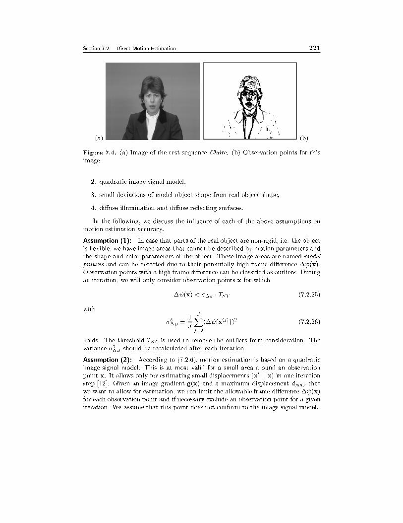
Section 7.2. Direct Motion Estimation 221
(a) (b)
Figure 7.4. (a) Image of the test sequence Claire. (b) Observation points for this
image
2. quadratic image signal model,
3. small deviations of model object shape from real object shape,
4. di�use illumination and di�use re ecting surfaces.
In the following, we discuss the in uence of each of the above assumptions on
motion estimation accuracy.
Assumption (1): In case that parts of the real object are non-rigid, i.e. the object
is exible, we have image areas that cannot be described by motion parameters and
the shape and color parameters of the object. These image areas are named model
failures and can be detected due to their potentially high frame di�erence � (x).
Observation points with a high frame di�erence can be classi�ed as outliers. During
an iteration, we will only consider observation points x for which
� (x) < �� � TST (7.2.25)
with
�2� =
1
J
JXj=0
(� (x(j)))2 (7.2.26)
holds. The threshold TST is used to remove the outliers from consideration. The
variance �2� should be recalculated after each iteration.
Assumption (2): According to (7.2.6), motion estimation is based on a quadratic
image signal model. This is at most valid for a small area around an observation
point x. It allows only for estimating small displacements (x0 � x) in one iteration
step [12]. Given an image gradient g(x) and a maximum displacement dmax that
we want to allow for estimation, we can limit the allowable frame di�erence � (x)
for each observation point and if necessary exclude an observation point for a given
iteration. We assume that this point does not conform to the image signal model.
222 Three Dimensional Motion Estimation Chapter 7
Assumption (3): The shape di�erence between the model object and the real
object can be modeled by means of a spatial uncertainty of an observation point
along the line of sight. This can be considered using a Kalman �lter during motion
estimation [9].
Assumption (4): Although in uence of non-di�use illumination and re ections
disturb image analysis, they are usually not modeled separately. To some extent,
these image areas are automatically detected when detecting model failures (see
assumption 1)
Summarizing these observations, we conclude that we should select observation
points with large absolute image gradients according to Eq. (7.2.24). Only observa-
tion points that pass this initial test will be considered during motion estimation.
Eq. (7.2.25) provides a selection criterion for the observation points that we will use
for a given iteration step. In [13], further details on robust direct motion estimation
and maximum-likelihood estimation are discussed. In the following, we will brie y
focus on an eÆcient estimator described in [13] and [7].
Instead of using the binary selection criteria for observation points according to
Eq. (7.2.25), we can use continuous cost functions to control the in uence of an
observation point on the parameter estimation. We use the residual rj according to
Eq. (7.2.10) as measure for the in uence of an observation point [14][23]. A critical
point for selecting an appropriate measure is the treatment of outliers. Ideally,
we would know the probability density function of the outliers. Furthermore, we
want outliers to have no in uence on the estimated motion parameters. However,
the probability density function of outliers is often unknown. Therefore heuristic
solutions using the cost function w = (1�r2=b2)2 as suggested by Tukey were found
[7][23]:
r0
j =
(rj �
�1�
r2j
b2
�if jrj j < b
0 otherwise.(7.2.27)
Instead ofPj jrj j
2! min we now minimize
Xj
jrj j2jwj j
2! min: (7.2.28)
The cost w = (1 � r2=b
2)2 increases to 1 when jrj decreases. Observation points
with jrj j � b are excluded from the next iteration. The constant b is the threshold
for detecting outliers. In order to adapt the outlier detection to the image di�erence
signal � we select b proportional to �� in Eq. (7.2.26). During motion estimation,
we multiply the equation of each observation point x(j) with its individual cost wj =
(1 � r2j =b
2)2 therefore adapting its in uence on the estimated motion parameters
according to Eq. (7.2.11) and Eq. (7.2.20).
Section 7.3. Iterative Motion Estimation 223
7.3 Iterative Motion Estimation
Direct motion estimation algorithms can only estimate small motion, mainly due
to the limited range for which the assumptions of the image signal model hold. In
order to estimate larger motion, we have to use an iterative algorithm.
Let us assume that we estimate the motion parameters starting with a set of ob-
servation points and equations as described in one of the previous sections. During
this �rst iteration we solve for the motion parameters Ri and Ti with i = 1 giving
the residual ri. We use these motion parameters to motion compensate the object
and its observation points. If appropriate, we use the non-linear motion equations
for motion compensation even if the motion parameters are solved by using a lin-
earized rotation matrix. We now set up a new set of equations following the same
procedure as for iteration 1 resulting in the motion parameters Ri and Ti with
i = 2. We continue these iterations as long as the new motion parameters decrease
the residual, i.e. (r2j � r2j+1) > T with threshold T chosen appropriately. The �nal
estimated motion parameters from image k to image k + 1 can be computed by
concatenating the motion parameters of each iteration.
To show the principle of motion parameter concatenation, we compute the mo-
tion parameter concatenation for the algorithm presented in Section 7.2.2. Assum-
ing motion according to Eq. (5.3.9), the estimated rotation matrix [R] becomes
[R] = �Ii=1[RI+1�i] (7.3.1)
with the rotation matrix [Ri] estimated in iteration i. The computation of the
translation vector T has to consider the center of rotation. Assuming that we
compute rotation around Ci during iteration i, we get
T = TI +CI + [RI ] (TI�1 +CI�1 �CI + [RI�1](TI�2 +CI�2 �CI�1 + � � �))
(7.3.2)
assuming rotation around the coordinate center, i.e. the object moves according to
X0 = [R]X+ T: (7.3.3)
Compared to indirect motion estimation, direct motion estimation usually re-
quires iterative algorithms that tend to be more compute intensive. However, direct
motion estimation has the advantage of considering the image signal during estima-
tion.
7.4 Summary
In this chapter, we discussed several methods of estimating 3D motion. We pre-
sented two estimation methods, indirect motion estimation and direct motion esti-
mation.
Indirect motion estimation algorithms (Sec. 7.1) depend on feature points on the
moving object. The feature points have to be reliably marked on two images. Then
224 Three Dimensional Motion Estimation Chapter 7
we can estimate 3D motion from these correspondences. The algorithms allow for
estimating large motion. However, the estimation algorithms tend to be sensitive
to errors in the feature point correspondences. Di�erent algorithms can be used
depending on whether we want to assume orthographic (Sec. 7.1.1) or perspective
(Sec. 7.1.2, 7.1.4) projection and whether we know the object shape. Using an
orthographic camera model is acceptable if the object does not move signi�cantly
in the direction of the camera axis and object rotation is mainly within the camera
plane. Otherwise we use an algorithm with a perspective camera model, which
requires more computations than an orthographic model. Estimating the essential
matrix from feature point correspondences (Sec. 7.1.4) enables us to determine the
motion of the object as well as the 3D location of these feature points. In order
to gain robustness against noise, we suggest to use the epipolar line constraint
and minimize the distance of the feature points from this line (Eq. 7.1.34) when
determining the motion and shape parameters from the essential matrix.
Direct motion estimation algorithms (Sec. 7.2) approximate the image signal
using a Taylor series expansion (Section 7.2.1) and derive pel-based motion (optical
ow) from the frame di�erence signal. This pel-based motion is used directly to
compute the 3D motion parameters. The algorithms are used if we have small
object motion from one frame to another. The motion estimation range can be
extended using an iterative approach (Sec. 7.3). Usually, we are required to make
some assumption about the 3D object shape. The algorithm described in Sec. 7.2.3
assumes a planar object shape. Key to the successful use of direct motion estimation
algorithms is the careful selection of those observation points where we measure the
frame di�erence signal. In Sec. 7.2.4 we describe robust methods for selecting these
points during motion estimation.
The selection of the estimation method depends to a large extend on what
measurements are available. Indirect motion estimation is the method of choice if
we have only a few highly accurate feature point locations. Direct motion estimation
should be used if we can reliably estimate motion from the image signal using optical
ow. As always, a combination of these approaches might results in the best results
for some applications.
7.5 Problems
1. What are the di�erences between a direct and an indirect motion estimator.
What are the potential advantages and disadvantages?
2. Derive Eq. (7.1.9). Start with the general 3D motion equationX0 = [R]X+T
and the plane equation in Eq. (7.1.8).
3. Show that Eq. (7.1.10) can be written as Eq. (7.1.11).
4. Show that the solution to the optimization problem in Eq. (7.1.22) is the unit
eigenvector of ATA associated with the smallest eigenvalue.
Section 7.6. Bibliography 225
5. Consider an image point x that is the projection of X. This point moves to x0
and X 0, respectively. Derive the epipolar line for this point x for the motion
parameters T and [R]. For an image point x and its epipolar line, compute
and draw a curve that shows how the distance of a point X from the camera
center determines its location on the epipolar line?
6. When estimating the E-matrix, the in uence of a measurement error Æ in
the point correspondence depends on the absolute coordinates of these cor-
respondences. Show how the residual of a point correspondence depends on
the coordinates of the corresponding points. In Eq. (7.1.11) and Eq. (7.1.19)
replace x0 by x0+Æ. What would be the weighting factors for each equation in
(7.1.22) such that the image coordinates of a correspondence do not in uence
the estimation of the E-matrix?
7. Present a polynomial representation of the luminance signal (x) around x
using a linear and a quadratic image signal model.
8. Derive Eq. (7.2.6) and Eq. (7.2.5) using a second order Taylor series expansion
for the image signal.
9. In order to implement the direct motion estimation algorithm for planar ob-
jects (Section 7.2.3), the inverse mapping of A has to be known. Show that
the mapping A ful�lls the four axioms of a group, namely closure, existence
of an inverse, existence of an identity and associativity. Compute the inverse
of a mapping A and the sum of the motion parameter estimates after two
iterations.
10. Discuss measures to increase the robustness of a direct motion estimation
algorithm.
7.6 Bibliography
[1] K. Aizawa, H. Harashima, and T. Saito. Model-based analysis-synthesis image
coding (MBASIC) system for a person's face. Signal Processing: Image Commun.,
1(2), October 1989.
[2] P. Beardsley, P. H. S. Torr, and A. Zisserman. 3D model aquisition from ex-
tended image sequences. In B. Buxton and Cipolla R., editors, Proc. 4th European
Conference on Computer Vision, LNCS 1065, pages 683{695. Springer{Verlag,
1996.
[3] M. Bierling. Displacement estimation by hierarchical block matching. In Proc.
SPIE: Visual Commun. Image Processing, volume SPIE-1001, pages 942{951,
Cambridge, MA, Nov. 1988.
226 Three Dimensional Motion Estimation Chapter 7
[4] G. Bozdagi, A. M. Tekalp, and L. Onural. An improvement to mbasic algorithm
for 3-D motion and depth estimation. IEEE Trans. Image Process., 3:711{716,
June 1994.
[5] M. H�otter and R. Thoma. Image segmentation based on object oriented mapping
parameter estimation. Signal Processing, 15(3):315{334, October 1988.
[6] T.S. Huang and A.N. Netravali. Motion and structure from feature correspon-
dences: A review. Proceedings of the IEEE, 82(2):252{268, February 1004. Feature,
general overview, estimation methods.
[7] H. Li and R. Forchheimer. Two-view facial movement estimation. IEEE trans
on circuits and systems for video technology, 4(3):276{287, June 1994.
[8] H.C. Longuet-Higgins. A computer algorithm for reconstructing a scene from
two projections. Nature, 293(5828):133{5, September 1981.
[9] G. Martinez. Shape estimation of articulated 3D objects for object-based
analysis-synthesis coding (OBASC). Signal Processing: Image Communication,
9(3):175{99, March 1997.
[10] P. Meer, D. Mintz, and D.Y. Kim. Robust regression methods in computer
vision: a review. International Journal of Computer Vision, 6(1):59{70, April
1991.
[11] T. Moons. A guided tour through multiview relations. In Proceedings SMILE
Workshop, LNCS 1506, pages 304{346. Springer, 1998.
[12] H.G. Musmann, P. Pirsch, and H.-J. Grallert. Advances in picture coding.
Proceedings of the IEEE, 73(4):523{548, Apr. 1985.
[13] J. Ostermann. Object-based analysis-synthesis coding based on moving 3D
objects. In L. Guan, S. Y. Kung, and J. Larsen, editors, Multimedia Image and
Video Processing. CRC Press, 2000.
[14] W. H. Press, S.A. Teukolsky, W. T. Vetterling, and B. P. Flannery. Numerical
Recipes in C: The Art of Scienti�c Computing. Cambridge University Press, 1992.
[15] P.J. Rousseeuw and A.M. Leroy. Robust Regression and Outlier Detection.
John Wiley & Sons, New York, 1987.
[16] J. Stauder. Estimation of point light source parameters for object-based coding.
Signal processing: Image Communication, 46(7):355{379, 1995.
[17] R. Y. Tsai and T. S. Huang. Uniqueness and estimation of three-dimensional
motion parameters of rigid objects with curved surfaces. IEEE Trans. Pattern
Anal. Machine Intell., PAMI-6:13{16, Jan. 1981.
Section 7.6. Bibliography 227
[18] R.Y. Tsai and T.S. Huang. Estimating three-dimensional motion parameters
of a rigid planar patch. IEEE Transactions on Acoustics, Speech and Signal Pro-
cessing, ASSP-29(6):1147{52, Dec 1981.
[19] R.Y. Tsai and T.S. Huang. Uniqueness and estimation of three-dimensional
motion parameters of rigid objects with curved surfaces. IEEE Transactions on
Pattern Analysis and Machine Intelligence, PAMI-6(1):13{27, Jan 1984.
[20] R.Y. Tsai, T.S. Huang, and Wei-Le Zhu. Estimating three-dimensional motion
parameters of a rigid planar patch. ii. singular value decomposition. IEEE Trans-
actions on Acoustics, Speech and Signal Processing, ASSP-30(4):525{34, August
1982.
[21] J. Weng, T.S. Huang, and N. Ahuja. Motion and structure from two perspective
views: algorithms, error analysis, and error estimation. IEEE Transactions on
Pattern Analysis and Machine Intelligence, 11(5):451{76, May 1989.
[22] X.Zhuang. A simpli�cation to linear 2-view motion algorithms. Computer
Vision Graphics and Image Processing, 46(2):175{178, 1989.
[23] X. Zhuang, T. Wang, and P. Zhang. A highly robust estimator through par-
tially likelihood function modeling and its application in computer vision. IEEE
Transactions on pattern analysis and machine intelligience, 14(1):19{34, Januar
1992.
Chapter 8
FOUNDATIONS FOR VIDEO
CODING
Video coding is an important application of digital video processing. The goal of
video coding is to reduce the data rate of a video sequence so that it is feasible to
transmit the video in real-time over a given communication channel. The channel
bandwidth varies depending on the application and the transmission media. For
video phone applications using regular telephone lines, 20 Kbit/s may be all that
is available for video coding. For broadcasting of standard de�nition television
signals over satellite, a data rate of 6 Mbit/s may be available. In addition to com-
munications applications, video coding is also necessary for storage and retrieval
applications, where di�erent storage media have di�erent capacity and access rates,
thus demanding varying amount of compression. Due to this wide range of data
rates, di�erent algorithms have been developed. One class of algorithms allows eÆ-
cient coding of arbitrary video signals without trying to analyze the video content.
A second class of algorithms identi�es regions and objects in a video sequence and
codes those. We call the former a waveform-based video coder and the latter a
content-dependent video coder.
In this chapter, we �rst give an overview of di�erent waveform-based and content-
dependent video coders in Sec. 8.1. Then, following a review of basic probability
and information theory concepts in Sec. 8.2, information theory used to optimize
lossless coding and rate distortion theory used to optimize lossy coding are intro-
duced in Sec. 8.3. This will be followed by description of lossless coding (Sec. 8.4)
and the most basic lossy coding techniques including scalar and vector quantization
(Secs. 8.5 and 8.6). Chapters 9 and 10 will discuss techniques for waveform-based
video coding and content-dependent video coding, respectively.
8.1 Overview of Coding Systems
8.1.1 General Framework
The components of a video coding algorithm are determined to a large extent by
the source model that is adopted for modeling the video sequences. The video
228
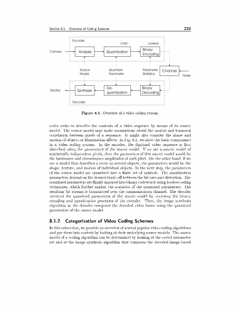
Section 8.1. Overview of Coding Systems 229
Analysis
Source
Model
QuantizationBinary
Encoding
SynthesisDe-
quantization
Binary
Decoding
Quantizer
Parameter
Parameter
StatisticsChannel
Noise
Camera
Monitor
Lossy LosslessEncoder
Decoder
Figure 8.1. Overview of a video coding system.
coder seeks to describe the contents of a video sequence by means of its source
model. The source model may make assumptions about the spatial and temporal
correlation between pixels of a sequence. It might also consider the shape and
motion of objects or illumination e�ects. In Fig. 8.1, we show the basic components
in a video coding system. In the encoder, the digitized video sequence is �rst
described using the parameters of the source model. If we use a source model of
statistically independent pixels, then the parameters of this source model would be
the luminance and chrominance amplitudes of each pixel. On the other hand, if we
use a model that describes a scene as several objects, the parameters would be the
shape, texture, and motion of individual objects. In the next step, the parameters
of the source model are quantized into a �nite set of symbols. The quantization
parameters depend on the desired trade-o� between the bit rate and distortion. The
quantized parameters are �nally mapped into binary codewords using lossless coding
techniques, which further exploit the statistics of the quantized parameters. The
resulting bit stream is transmitted over the communication channel. The decoder
retrieves the quantized parameters of the source model by reversing the binary
encoding and quantization processes of the encoder. Then, the image synthesis
algorithm at the decoder computes the decoded video frame using the quantized
parameters of the source model.
8.1.2 Categorization of Video Coding Schemes
In this subsection, we provide an overview of several popular video coding algorithms
and put them into context by looking at their underlying source models. The source
model of a coding algorithm can be determined by looking at the coded parameter
set and at the image synthesis algorithm that composes the decoded image based
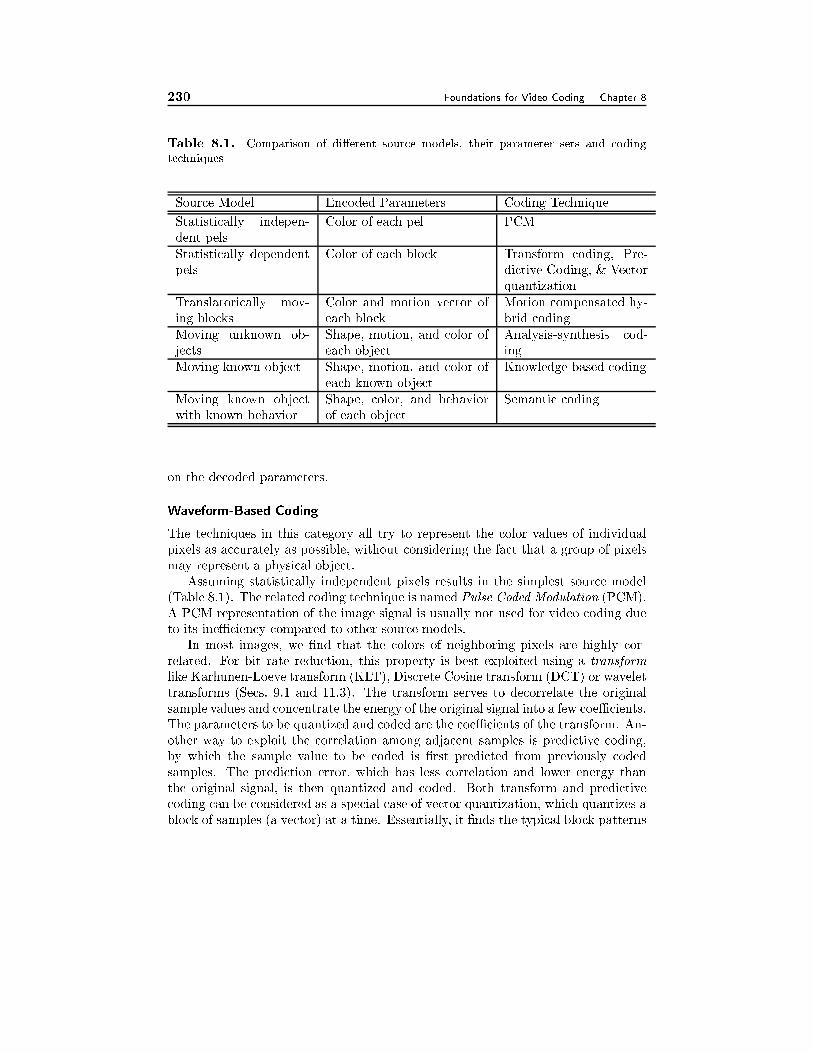
230 Foundations for Video Coding Chapter 8
Table 8.1. Comparison of di�erent source models, their parameter sets and coding
techniques
Source Model Encoded Parameters Coding Technique
Statistically indepen-
dent pels
Color of each pel PCM
Statistically dependent
pels
Color of each block Transform coding, Pre-
dictive Coding, & Vector
quantization
Translatorically mov-
ing blocks
Color and motion vector of
each block
Motion compensated hy-
brid coding
Moving unknown ob-
jects
Shape, motion, and color of
each object
Analysis-synthesis cod-
ing
Moving known object Shape, motion, and color of
each known object
Knowledge-based coding
Moving known object
with known behavior
Shape, color, and behavior
of each object
Semantic coding
on the decoded parameters.
Waveform-Based Coding
The techniques in this category all try to represent the color values of individual
pixels as accurately as possible, without considering the fact that a group of pixels
may represent a physical object.
Assuming statistically independent pixels results in the simplest source model
(Table 8.1). The related coding technique is named Pulse Coded Modulation (PCM).
A PCM representation of the image signal is usually not used for video coding due
to its ineÆciency compared to other source models.
In most images, we �nd that the colors of neighboring pixels are highly cor-
related. For bit rate reduction, this property is best exploited using a transform
like Karhunen-Loeve transform (KLT), Discrete Cosine transform (DCT) or wavelet
transforms (Secs. 9.1 and 11.3). The transform serves to decorrelate the original
sample values and concentrate the energy of the original signal into a few coeÆcients.
The parameters to be quantized and coded are the coeÆcients of the transform. An-
other way to exploit the correlation among adjacent samples is predictive coding,
by which the sample value to be coded is �rst predicted from previously coded
samples. The prediction error, which has less correlation and lower energy than
the original signal, is then quantized and coded. Both transform and predictive
coding can be considered as a special case of vector quantization, which quantizes a
block of samples (a vector) at a time. Essentially, it �nds the typical block patterns
Section 8.1. Overview of Coding Systems 231
occurring in the signal and approximates any block by one of the typical patterns.
Today's video coding standards, H.261, H.263, MPEG-1, MPEG-2, and MPEG-
4 (Chap. 13), are based on motion-compensated hybrid coding, which combines pre-
dictive coding with transform coding (Sec. 9.2.4). This coding technique subdivides
each image into �xed sized blocks. Each block of a frame k is synthesized using a
block of the same size at a displaced position of the previous frame k-1. This is done
for all blocks of frame k. The resulting image is called the predicted image. The
encoder transmits the 2-D motion vectors for all blocks to the decoder such that
the decoder can compute the same predicted image. The encoder subtracts this
predicted image from the original image, resulting in the prediction error image.
If the synthesis of a block using the predicted image is not suÆciently accurate,
i.e., the prediction error of a block exceeds a threshold, then the encoder uses a
transform coder for transmitting the prediction error of this block to the decoder.
The decoder adds the prediction error to the predicted image and thus synthesizes
the decoded image. Therefore, motion compensated hybrid coding is based on the
source model of translatorically moving blocks. In addition to the color information
encoded as transform coeÆcients of the prediction error, motion vectors have to be
transmitted. It is worth noting that such a coder can switch to the simpler source
model of statistically dependent pixels. This is done whenever the coding of a block
is achieved more eÆciently without referring to the previous frame.
Content-Dependent Coding
The above block-based hybrid coding techniques essentially approximate the shape
of objects in the scene with square blocks of �xed size. Therefore, this coder gener-
ates high prediction errors in blocks on object boundaries. These boundary blocks
contain two objects with di�erent motions, which cannot be accounted for by a
single motion vector. Content-dependent coders recognize such problems, and try
to segment a video frame into regions corresponding to di�erent objects and code
these objects separately. For each object, shape information has to be transmitted
in addition to motion and texture information.
In object-based analysis-synthesis coding (OBASC) (Sec. 10.5), each moving ob-
ject of the video scene is described by a model object. In order to describe the
shape of an object, OBASC employs a segmentation algorithm. Further, motion
and texture parameters of each object are estimated. In the simplest case, a 2-D
silhouette describes the shape of an object, a motion vector �eld describes its mo-
tion, and the color waveform represents its texture. Other approaches describe an
object with a 3-D wireframe. An object in frame k is described by the shape and
color of an object in frame k-1 and an update of shape and motion parameters. The
decoder synthesizes the object using the current motion and shape parameters as
well as the color parameters of the preceding frame. Only for those image regions
where the image synthesis fails, color information is transmitted.
In the case that the object type in a video sequence belongs to some known object
classes, knowledge-based coding can be employed, which uses a wireframe specially
232 Foundations for Video Coding Chapter 8
designed to describe the recognized object type (Sec. 10.6). Several approaches
have been developed to code human heads using prede�ned wireframes. Using a
prede�ned wireframe increases coding eÆciency because it is adapted to the shape
of the object. Sometimes, this technique is also referred to as model-based coding.
When possible object types as well as their behaviors are known, semantic coding
may be used. For example, for a human face object, the behavior refers to the
temporal trajectory of a set of facial feature points associated with a particular
facial expression. The possible behaviors of a human face include typical facial
expressions such as happiness, sadness, anger, etc. In this case, the parameters for
describing the behavior of an object are estimated and transmitted to the decoder.
This coding technique has the potential for achieving very high coding eÆciency,
because the number of possible behaviors for an object like a face is very small, and
the number of bits required to specify the behavior is much smaller than that for
describing the actual action with conventional motion and color parameters.
8.2 Basic Notions in Probability and Information Theory
In video coding or coding of any signal, we treat a given signal as the realization of a
random process. In source coding theory, a random process is referred to as a source.
The eÆciency of a coding technique depends on how fully the source statistics are
exploited. Before moving into the theory and techniques for source coding, we �rst
review how to characterize a random process using probability distributions, and
introduce the concepts of entropy and mutual information from information theory.
8.2.1 Characterization of Stationary Sources
We only consider sources de�ned over a discrete index set so that a source is a
random sequence. We use F = fFng to represent a source, in which Fn represent
the random variable (RV) corresponding to the n-th sample. The actual value that
Fn takes in a given realization is denoted by fn. Note that for a discrete signal
over a multi-dimensional space, we can either order it into a 1-D sequence, so that n
refers to the 1-D index of a sample, or we can assume n is a multi-dimensional index.
Also, Fn can be a scalar or a vector. In the latter case, it is also called a random
vector. If Fn can only take symbols from a �nite alphabet A = fa1; a2; : : : ; aLg,then we call Fn a discrete RV and F a discrete source. If Fn takes value over a
continuous supporting range or the union of several continuous ranges, denoted by
B, then Fn is called a continuous RV and F a continuous source.1
As an example, consider a digital color video. In this case, the index n represents
a particular combination of pixel location and frame number, and Fn is a 3-D
random vector, representing the three color values taken by the n-th pixel. Because
each color value is quantized into 256 levels, a digital video is a discrete source with
1Note that in this chapter, the word \discrete" and \continuous" refer to the sample amplitude,
whereas in earlier chapters, they refer to the space over which the signal is de�ned. A digital signal
is a discrete space signal in which each sample takes only discrete values.
Section 8.2. Basic Notions in Probability and Information Theory 233
an alphabet size of 2563. Any given video sequence is a particular realization of
this discrete random process. An analog video, on the other hand, is a continuous
space continuous amplitude random process. The sampling process converts it to a
discrete space continuous amplitude process. Only after quantization, it becomes a
discrete space discrete amplitude process (i.e., a discrete source). In the real world,
a discrete source is often obtained from a continuous space continuous amplitude
source by sampling and quantization.
In this book, we only consider stationary processes, in which the probability
distribution of Fn does not depend on the index n, and the joint distribution of a
group of N samples is invariant with respect to a common shift in the index. In this
case, we use pFn(f) to represent the probability mass function (pmf), in the case of a
discrete source, or the probability density function (pdf), in the case of a continuous
source, of any sample Fn. In addition, we use pFn+1;Fn+2;:::;Fn+N (f1; f2; : : : ; fN )
to represent the joint pmf or pdf of any N successive samples in F . We also use
pFnjFn�1;Fn�2;:::;Fn�M (fM+1jfM ; fM�1; : : : ; f1) to represent the conditional pmf or
pdf of any sample Fn given its previousM samples. When it is clear from the under-
lying context, we simply use p(f); p(f1; f2; : : : ; fN); and p(fM+1jfM ; fM�1; : : : ; f1)
to denote the above functions.
An important class of stationary sources is known as independent and identically
distributed (i.i.d.) sources, which satisfy p(f1; f2; : : : ; fN ) = p(f1)p(f2) � � � p(fN ),and p(fM+1jfM ; fM�1; : : : ; f1) = p(fM+1): An i.i.d. source is also referred to as
memoryless. Another important class is the Markov process, in which a sam-
ple only depends on its immediate predecessor, i.e., p(fM+1jfM ; fM�1; : : : ; f1) =
p(fM+1jfM ): More generally, an M-th order Markov process is the one in which a
sample only depends on its previousM samples. A process in which any N samples
follow an N -th order Gaussian distribution is called a Gaussian process. A Gaus-
sian process is Markov if the covariance between two samples Fn and Fm has the
form C(Fn;Fm) = �2��(n�m): Such a process is called a Gauss-Markov process,
or a Gauss-Markov �eld (GMF) when the underlying process is two dimensional.
In image and video processing, a real image or video frame is often modeled as a
GMF.
8.2.2 Entropy and Mutual Information for Discrete Sources
In this section, we introduce two very important notions from information theory:
entropy and mutual information. As will be seen later, they provide bounds on
the minimal bit rates achievable using lossless and lossy coding, respectively. We
�rst de�ne entropy and mutual information for discrete RVs, and then apply these
de�nitions to samples in a discrete source.
De�nition 8.1 (Entropy of a Discrete RV) The entropy of a discrete RV Fwith an alphabet A and a pmf pF (f) is de�ned by
H(F) = �Xf2A
pF(f) log2 pF(f): (8.2.1)
234 Foundations for Video Coding Chapter 8
In general, the log can be taken to any base. Here we only consider the base-2
case, so that entropy is expressed in bits. Also, it is assumed that 0 log 0 = 0; so
that adding a symbol with zero probability to the alphabet does not change the
entropy.
The entropy of a discrete RV is always non-negative, because 0 � p(f) � 1
for any pmf. Among all RVs with an alphabet size L, the uniform distribution,
p(f) = 1=L; f 2 A; achieves the maximum entropy, Hmax = log2 L:
Entropy is a measure of the uncertainty about a RV F . It depends on the pmf
of F , not the actual alphabet used by F . When F can take on any value in Awith equal probability, it is most uncertain, hence it has maximum entropy. On
the other hand, if F takes a particular symbol in A with probability 1, it has no
uncertainty, and hence the entropy is zero. The uncertainty about a RV can in turn
be considered as the information that may be conveyed by a RV: when one is shown
the actual value taken by F , one is told a lot more in the �rst case than in the
second.
De�nition 8.2 (Joint Entropy of Two Discrete RVs) Let F and G represent
two discrete RVs, with a joint pmf pF;G(f; g); f 2 Af ; g 2 Ag. Their joint entropy
is de�ned as
H(F ;G) = �Xf2Af
Xg2Ag
pF;G(f; g) log2 pF;G(f; g): (8.2.2)
De�nition 8.3 (Conditional Entropy between Two Discrete RVs) Let F and
G represent two discrete RVs, with marginal pmf pG(g) and conditional pmf pFjG(f jg); f 2Af ; g 2 Ag. The conditional entropy of F given G is de�ned as
H(FjG) =Xg2Ag
pG(g)H(Fjg)
= �Xg2Ag
pG(g)Xf2Af
pFjG(f jg) log2 pFjG(f jg): (8.2.3)
De�nition 8.4 (Mutual Information between Two Discrete RVs) Let F and
G represent two discrete RVs, with a joint pmf pF;G(f; g); f 2 Af ; g 2 Ag and
marginal distributions pF (f) and pG(g). The mutual information between F and Gis de�ned as
I(F ;G) =Xf2Af
Xg2Ag
pF;G(f; g) log2pF;G(f; g)
pF(f)pG(g): (8.2.4)
The mutual information between F and G speci�es the amount of information
provided by G about F : In other words, it measures the reduction in the number
of bits required to specify F , given the realization of G: The mutual information is
always non-negative. It is easy to show that
I(F ;G) = I(G;F) � 0: (8.2.5)
Section 8.2. Basic Notions in Probability and Information Theory 235
Relations between Entropy, Conditional Entropy, and Mutual Information We
summarize some important relations between entropy, conditional entropy and mu-
tual information below. These relations can be proved quite easily (Prob. 8.2).
H(F ;G) = H(G) +H(FjG) = H(F) +H(GjF) (8.2.6)
I(F ;G) = H(F)�H(FjG) = H(G)�H(GjF) (8.2.7)
I(F ;G) = H(F) +H(G)�H(F ;G) (8.2.8)
I(F ;G) � H(F); I(F ;G) � H(G) (8.2.9)
H(F) � H(FjG); H(G) � H(GjF) (8.2.10)
H(F ;G) � H(F) +H(G) (8.2.11)
I(F ;F) = H(F) = H(F ;F) (8.2.12)
Equation (8.2.10) says that conditioning reduces the entropy (i.e., uncertainty)
of a RV. From Eq. (8.2.7), we can see that I(F ;G) describes the reduction in the
uncertainty (or information) of F due to the knowledge of G.The above de�nitions are given for a RV or between two RVs. They can be
similarly de�ned for random vectors. By applying these de�nitions to random
vectors consisting of successive samples in a discrete stationary source, we arrive at
the following de�nitions.
De�nition 8.5 (Entropy of a Discrete Source) The N-th order entropy of a
discrete stationary source F with N-th order joint pmf p(f1; f2; : : : ; fN) is the joint
entropy among N successive samples F1;F2; : : : ;FN of F :
HN (F) = H(F1;F2; : : : ;FN )= �
X[f1;f2;:::;fN ]2AN
p(f1; f2; : : : ; fN ) log2 p(f1; f2; : : : ; fN ); (8.2.13)
where ANrepresents the N-fold Cartesian product of A.
De�nition 8.6 (Conditional Entropy of a Discrete Source) TheM-th order
conditional entropy of a discrete stationary source F with M-th order joint pmf
p(f1; f2; : : : ; fM ) and M-th order conditional pmf p(fM+1jfM ; fM�1; : : : ; f1) is theconditional entropy of a sample FM+1 given its previousM samples FM ;FM�1; : : : ;F1:
Hc;M(F) = H(FM+1jFM ;FM�1; : : : ;F1)
=X
[f1;f2;:::;fM ]2AM
p(f1; f2; : : : ; fM )H(FM+1jfM ; fM�1; : : : ; f1) (8.2.14)
where
H(FM+1jfM ; fM�1; : : : ; f1) =
�X
fM+12A
p(fM+1jfM ; fM�1; : : : ; f1) log2 p(fM+1jfM ; fM�1; : : : ; f1): (8.2.15)
236 Foundations for Video Coding Chapter 8
De�nition 8.7 (Entropy Rate of a Discrete Source) It can be shown that1NHN (F)
and Hc;N(F) are both non-increasing function of N . Furthermore, limN!11NHN (F)
and limN!1Hc;N(F) both exist and are equal. This limit is de�ned as the entropy
rate of the source:
�H(F) = limN!1
1
NHN (F) = lim
N!1Hc;N(F): (8.2.16)
Relation between joint entropy, conditional entropy and entropy rate It can be
shown (Prob. 8.3) that, for any �nite N and M ,
HN (F) =
N�1Xm=1
Hc;m(F) +H1(F) (8.2.17)
�H(F) � Hc;N�1(F) � 1
NHN (F) � H1(F); (8.2.18)
If F is i.i.d., then
�H(F) =1
NHN (F) = Hc;M (F) = H1(F): (8.2.19)
As will be shown in Sec. 8.3.1, the entropy rate is the lower bound on the minimal
bit rate required to code a discrete source losslessly. The bound can be achieved
only when an in�nite number of samples are coded together. On the other hand, the
�rst order entropy and conditional entropy provide lower bounds on the achievable
bit rate when one sample is coded independently, or conditioned on the previous
samples.
De�nition 8.8 (Mutual Information between Discrete Sources) Let F and
G represent two discrete stationary sources, with N -th order pmf p(f1; f2; : : : ; fN )
and p(g1; g2; : : : ; gN), respectively. Further let p(f1; f2; : : : ; fN ; g1; g2; : : : ; gN ) rep-
resent the joint pmf of N samples each from F and G. The N-th order mutual
information between F and G is de�ned as
IN (F ;G) =X
[f1;f2;:::;fN ]2AN
f
X[g1;g2;:::;gN ]2AN
g
p(f1; f2; : : : ; fN ; g1; g2; : : : ; gN ) �
log2p(f1; f2; : : : ; fN ; g1; g2; : : : ; gN)
p(f1; f2; : : : ; fN )p(g1; g2; : : : ; gN )(8.2.20)
In lossy source coding, a source F = fFng is represented by a quantized version
G = fGng. The �rst order mutual information I1(F ;G) measures the amount
of information provided by a quantized sample Gn about the original sample Fn.On the other hand, IN (F ;G) measures the information provided by a block of
N quantized samples about original N samples. As will be shown in Sec. 8.3.2,
limN!1min 1NIN (F ;G) provides a lower bound on the minimal bit rate required
for a desired distortion D between F and G; where the minimum is taken over all
possible G's that have distortion D from F .
Section 8.2. Basic Notions in Probability and Information Theory 237
8.2.3 Entropy and Mutual Information for Continuous Sources
For a continuous source, the pmf for any possible value in its support region is zero.
Direct application of the previously de�ned entropy would yield an in�nite entropy.
Instead, we use the pdf of the source to de�ne di�erential entropy.2
De�nition 8.9 (Di�erential Entropy of a Continuous RV) The di�erential en-
tropy of a continuous RV F with a support range B and a pdf pF (f) is de�ned by
h(F) = �Zf2B
pF(f) log2 pF(f)df: (8.2.21)
As with entropy, di�erential entropy measures the uncertainty or information
content of a continuous RV. Unlike entropy, di�erential entropy can take on negative
values and in fact can vary in the range of (�1;1), depending on the pdf.
All other de�nitions (including joint entropy, conditional entropy, mutual infor-
mation) given in Sec. 8.2.2 for discrete sources can be similarly given for continuous
sources, by replacing any involved pmf with a corresponding pdf. Similarly, the re-
lations between entropy, conditional entropy, and mutual information are still valid,
with entropy replaced by di�erential entropy.
Gaussian Sources
A very important continuous source is the Gaussian source, in which each sample
follows a Gaussian distribution and each group of N samples follows a joint Gaus-
sian distribution. Here, we give the di�erential entropy for a Gaussian RV and a
Gaussion random vector.
A Gaussian RV with mean � and variance �2 has a pdf
p(f) =1p2��
e�(f��)2=2�2 ; f 2 (�1;1): (8.2.22)
It can be shown (Problem 8.4) that its di�erential entropy is
hGaussian =1
2log2(2�e�
2): (8.2.23)
An N -dimensional Gaussian random vector F with mean � and covariance
matrix [C] has a joint pdf
p(f) =1
(p2�)N jdet[C]j1=2 exp
��1
2(f � �)T [C]
�1(f � �)
�: (8.2.24)
It can be shown that the di�erential entropy of this random vector (or joint di�er-
ential entropy among the N components) is
hN�DGaussian =1
2log2
�(2�e)N jdet[C]j� = 1
2log2
(2�e)N
Yn
�n
!; (8.2.25)
2The previously de�ned entropy based on the pmf is also known as absolute entropy.
238 Foundations for Video Coding Chapter 8
where �n; n = 1; 2; : : : ; N are the eigenvalues of [C]:
An important property of the Gaussian distribution is that the Gaussian RV has
the largest entropy among all continuous RVs with the same variance. Similarly,
a Gaussian random vector has the largest entropy among all random vectors with
the same covariance matrix. This makes the Gaussian source most diÆcult to code,
in that it requires a higher bit rate to represent than any other sources, for a given
distortion criterion.
8.3 Information theory for Source Coding
The theoretical foundation for source coding is established by several important
results of information theory.3 These results, due to Shannon, the father of infor-
mation theory, establish bounds on the minimal bit rate required to realize lossless
and lossy coding. A rigorous and comprehensive treatment of this subject is beyond
the scope of this book. The intent of this section is to help the reader to understand
the theoretical limits of source coding and how they may be used to guide the design
of practical coding techniques. The reader is referred to the books by Cover and
Thomas [3] and by Berger [1] for more in-depth exposition.
8.3.1 Bound for Lossless Coding
Scalar Lossless Coding
For a particular realization ffng of a discrete source F with an alphabet A =
fa1; a2; : : : ; aLg, scalar lossless coding refers to assigning a binary codeword cn for
each sample fn. This requires that one predesign a codebook C = fc(a1); c(a2); : : : ; c(aL)g,where c(ai) is the codeword for symbol ai: Then the codeword for fn will be
cn = c(fn). For a codebook to be useful, a coded sequence must be uniquely
decodable, i.e., a sequence of codewords corresponds to one and only one possible
sequence of source symbols. Note that this is a stronger requirement than the one
that the mapping between the alphabet and the codebook be one-to-one. Let l(ai)
denote the length (i.e., the number of bits) of c(ai), then the bit rate, de�ned as
the average number of bits per sample,4 will be equal to the average length per
codeword, i.e.,
R =Xai2A
p(ai)l(ai): (8.3.1)
3Source coding refers to the process of converting samples from a source into a stream of binary
bits, whereas channel coding refers to further manipulating the source bits to add protection against
transmission errors.4Elsewhere in this book, we also de�ne bit rate as the number of bits per second (bps). For a
source outputing fs sample/s and representing each sample with R bits, the bit rate in terms of
bps is fsR.
Section 8.3. Information theory for Source Coding 239
Theorem 8.1 (Bound for Scalar Lossless Coding) The minimum bit rate �R1(F)
required to represent a discrete stationary source F by assigning one codeword to
each sample satis�es
H1(F) � �R1(F) � H1(F) + 1: (8.3.2)
The lower bound can be achieved when the pmf of the source is a function of power
2. That is, there exist a set of integers fm1;m2; : : : ;mLg such that p(ai) = 2�mi :
In this case, l(ai) = � log2 p(ai) = mi:
The above theorem tells us that the �rst-order entropy of a discrete source
H1(F) determines the range of the minimum bit rate for scalar coding the source.
This is not surprising, as H1(F) measures the information content (in bit/sample)
carried by each new sample in a source.
Vector Lossless Coding
The above theorem tells us that, depending on the source, the minimal achievable
rate can be o� from the �rst order entropy by as much as 1 bit/sample. To further
reduce the bit rate, one can treat each successive N samples in a discrete sequence
as a vector-sample, and assign one codeword for each possible vector-symbol in
AN . The �rst order entropy of the vector source would be the N -th order entropy
of the original source. If �RN represent the minimal number of bits per vector, then
applying Theorem 8.1 to the above vector source yields
HN (F) � �RN (F) � HN (F) + 1 (8.3.3)
Let �RN = �RN=N represent the minimal number of bits per sample, we arrive at
the following theorem.
Theorem 8.2 (Bound for Vector Lossless Coding) The minimum bit rate �RN (F)
required to represent a discrete stationary source F by assigning one codeword to
each group of N successive samples satis�es
HN (F)=N � �RN (F) � HN (F)=N + 1=N: (8.3.4)
In the limit when N !1, from Eq. (8.2.16), we have
limN!1
�RN (F) = �H(F): (8.3.5)
The above theorem tells us that the bit rate can be made arbitrarily close to the
source entropy rate by coding many samples together.
Conditional Lossless Coding
We have seen that one can improve upon the eÆciency of scalar coding by vector
coding. An alternative is conditional coding, also known as context-based coding.
With M -th order conditional coding, the codeword for a current sample depends on
240 Foundations for Video Coding Chapter 8
the pattern formed by the previousM samples. Such a pattern is called the context.
Speci�cally, a separate codebook is designed for each possible context, based on the
conditional distribution of the output sample given this context. If the source
alphabet size is L, then the maximum number of contexts, and consequently the
maximum number of codebooks, is LM . Applying Theorem 8.1 to the conditional
distribution under context m, the minimal bit rate under this context satis�es
Hm
c;M (F) � �Rm
c;M (F) � Hm
c;M (F) + 1; (8.3.6)
where Hm
c;M(F) represents the entropy of the conditional distribution under context
m. Let pm represent the probability of context m, then the average minimal bit
rate with a conditioning order M is
�Rc;M (F) =Xm
pm �Rm
M (F): (8.3.7)
Substituting Eq. (8.3.6) to the above yields the following result.
Theorem 8.3 (Bound for Conditional Lossless Coding) The minimum bit rate
�Rc;M (F) required to represent a discrete stationary source F by using M-th order
conditional coding satis�es
Hc;M (F) � �Rc;M (F) � Hc;M (F) + 1: (8.3.8)
In the limit when M !1, we have
�H(F) � limM!1
�Rc;M (F) � �H(F) + 1: (8.3.9)
Compared to Eq. (8.3.2), conditional coding can achieve a lower bit rate than
scalar coding, because �H(F) < H1(F), unless the source is i.i.d. However, because
one still codes one sample at a time, the upper bound is still o� from the entropy rate
by 1 bit, even when the conditioning orderM goes to in�nity. ComparingN -th order
vector lossless coding with (N-1)-th order conditional coding, the former always has
the same or larger lower bound according to Eq. (8.2.18). On the other hand, vector
coding will have a smaller upper bound if 1NHN (F)�Hc;N�1(F) < N�1
N. Therefore,
which method is more eÆcient depends on the actual source statistics.
8.3.2 Bound for Lossy Coding*
When a source is continuous, it is impossible to represent it exactly with a �nite
number of bits. Recall that the absolute entropy rate of a continuous source is in�-
nite. Therefore, applying the bound on lossless coding (Eq. (8.3.5)) to a continuous
source leads to a minimal bit rate that is in�nite. To describe a continuous source
with a �nite number of bits, one must in some way quantize the source so that
each sample or a group of samples can only take symbols from a �nite alphabet.
Such quantization will inevitably induce distortion between the original source and
Section 8.3. Information theory for Source Coding 241
the reconstructed source based on the quantized representation. One can directly
quantize the source samples, either one at a time (scalar quantization) or a group
of samples together (vector quantization), or transform the samples into some other
parameters and quantize the resulting parameters. The quantized symbols can then
be encoded losslessly into binary codewords. At the decoder, the codewords are �rst
mapped back to the quantized symbols, from which each sample is reconstructed.
In general, a lossy coding process can be considered as mapping every input
vector f = ff1; f2; : : : ; fNg consisting of N samples from the original source F
into a quantized vector g = Q(f). The vector g must belong to a pre-designed
reconstruction codebook of a �nite size L, C = fg1;g2; : : : ;gLg: We will assume that
each component of f and g can only take values from the same support range B.Using �xed length coding, each quantized vector is represented by log2(L) bits, so
that the bit rate (bit/sample) of the coded sequence is
RN =1
Nlog2(L): (8.3.10)
Given a designed reconstruction codebook, the bit rate can be further reduced from
Eq. (8.3.10) by applying variable length coding to the indices of codewords. How-
ever, in the remaining discussions, we assume the bit rate is determined according
to Eq. (8.3.10).
To meet a given distortion criterion between F and G, the required codebook
size L depends on the coding scheme, i.e., how is the codebook designed. Intuitively,
the bit rate can be reduced by increasing the vector length N , especially when the
source is not i.i.d. The rate distortion theory de�nes the lower bound on the bit
rate required to achieve a given distortion, when N approaches in�nity.
Note that lossy coding can be applied to both continuous and discrete sources.
Recall that for a discrete source, the minimal bit rate required for lossless (zero
distortion) coding is bounded by the source entropy rate. To reach an even lower
rate, one must quantize the samples to a smaller alphabet, thereby incurring a
certain degree of distortion. The following discussions apply to both continuous
and discrete sources.
Distortion Measure
Until now, we have used the word \distortion" without formally de�ning it. To
measure the distortion between an original source F and the reconstructed source
G, we �rst de�ne a distortion measure d1(f; g) between two scalars f and g. When
f and g are both real values, the most common distortion measures are the squared
error, d1(f; g) = (f � g)2, and absolute error, d1(f; g) = jf � gj. Then the average
distortion per sample between an original vector f and the reconstructed one g is
dN (f ;g) =1
N
Xn
d1(fn; gn): (8.3.11)
The above distortion is de�ned for a given vector and its reconstruction vector.
To evaluate the average performance over all possible input vectors, we de�ne the
242 Foundations for Video Coding Chapter 8
following expected distortion between F and G when the vector length is N :
EfdN (F ;G)g =Zf2BN
Zg2BN
pN(f)qN (gjf)dN (f ;g)dfdg; (8.3.12)
where pN(f) represents the joint pdf of N successive samples in F , qN (gjf) rep-resents the conditional probability that f is reconstructed as g, BN represents the
N fold Cartesian product of B: Note that qN (gjf) essentially characterizes the cod-
ing scheme, although in practice, a deterministic mapping between f and g is used.
When d1(f; g) is the squared error, the above measure is known asmean square error
(MSE), which is widely used, primarily because of its mathematical tractability.
In the above, we have assumed the source is continuous, and the functions
pN (�); qN (�) represent pdf's. When the source is discrete, the integration over BNshould be placed by a sum over AN , and pN (�); qN (�) would represent correspondingpmf's.
Rate-Distortion Bound
The performance of a lossy coder is measured by its operational rate-distortion (RD)
function, denoted by R(D), which describes the bit rate R required to achieve
a given distortion D, for given source characteristics. The rate-distortion theo-
rem establishes the bound on the minimal rate required among all possible coders,
when the vector length N reaches in�nity. We call the function relating the mini-
mal rate and the distortion the rate-distortion (RD) bound, denoted by �R(D): Let
RN (D; qN (gjf)) represent the bit rate required to achieve distortion D by a coding
scheme described by qN (gjf). The RD bound is de�ned as
�R(D) = limN!1
minqN (gjf)2QD;N
RN (D; qN (gjf)) (8.3.13)
where
QD;N = fqN (gjf) : EfdN (F ;G)g � Dg (8.3.14)
is the set of conditional probabilities (i.e., coding schemes) that satisfy the speci�ed
distortion constraint.
Instead of representing R as a function of D, one can also representD in terms of
R, which will lead to the operational distortion-rate function D(R) or distortion-rate
bound �D(R).
Theorem 8.4 (Bound on Lossy Coding) The RD bound for coding a station-
ary source F at a distortion D is given by5
�R(D) = limN!1
minqN (gjf)2QD;N
1
NIN (F ;G): (8.3.15)
5In information theory, the RD function of a source F is de�ned as the right side of Eq. (8.3.15).
The Shannon source coding theorem states that there exists a coding scheme by which the bit rate
required to achieve a distortion D approaches �R(D).
Section 8.3. Information theory for Source Coding 243
When the source is i.i.d., the RD bound becomes
�R(D) = minq1(gjf)2QD;1
I1(F ;G): (8.3.16)
Recall that IN (F ;G) describes the amount of information provided by N sam-
ples of G about corresponding N samples of F : Therefore, it is not surprising that
IN (F ;G) determines the number of bits required to specify F with distortion D
when N !1:
An important result from information theory is that, even when the source is
i.i.d., one can reduce the bit rate R by coding many samples together. In fact, the
RD bound is achievable only when the vector length N reaches in�nity.
In general, the above bound is diÆcult to calculate for an arbitrary source. A
more useful bound is described by the following theorem.
Theorem 8.5: Under the MSE distortion criterion, the RD bound for any station-
ary source F satis�es
�RL(D) � �R(D) � �RG(D); (8.3.17)
where �RG(D) is the RD bound for a Gaussian source with the same variance as F ;
and �RL(D) is known as the Shannon lower bound, with
�RL(D) = �h(F)� 1
2log2 2�eD =
1
2log2
Q(F)
D; (8.3.18)
where �h(F) is the entropy rate of F , and Q(F) = 12�e
22�h(F )
is called the entropy
power of F : For a Gaussian source, �RL(D) = �RG(D):
The above theorem tells us that among all sources with the same variance, the
Gaussian source requires the highest bit rate, to satisfy the same distortion criterion.
In fact, for any source, the optimal coding scheme that achieves the RD bound is
the one by which the quantization error sequence is an i.i.d. Gaussian source with
variance D, with a di�erential entropy 12log2 2�eD. Therefore, the lower bound
given in Eq. (8.3.18) is equal to the di�erence between the di�erential entropy of
the original source and that of the quantization error.
8.3.3 Rate-Distortion Bounds for Gaussian Sources*
For most sources, a closed-form solution for the RD bound is diÆcult to derive. One
exception is the various types of Gaussian sources, for which closed-form solutions
have been found, when the distortion criterion is MSE. We summarize these results
below.
i.i.d. Gaussian source: The RD bound for an i.i.d. Gaussian source with variance
�2 is
�R(D) =
�12log2
�2
D; 0 � D � �2;
0; D > �2:(8.3.19)
Alternatively, one can write�D(R) = �22�2R: (8.3.20)
244 Foundations for Video Coding Chapter 8
i.i.d. Vector Gaussian Source with independent components: Consider an i.i.d.
vector Gaussian source, in which each vector sample consists of N independent
Gaussian RVs with variances �2n; n = 1; 2; : : : ; N . The RD bound for this source is
given by (R(�) = 1
N
Pnmaxf0; 1
2log2
�2n
�g;
D(�) = 1N
Pnminf�; �2
ng; (8.3.21)
where � is an intermediate parameter. The RD bound for the feasible distortion
region can be obtained by letting � traversing through the range (0;maxf�2ng):In the case when D is suÆciently small, so that D � minf�2
ng; the above reduces
to
�R(D) =1
2log2
�Qn�2n
�1=ND
; (8.3.22)
or�D(R) = (
Yn
�2n)1=N2�2R: (8.3.23)
The above RD bound is achieved by coding each component in a vector sample
independently,6 with Rn = maxf0; 12log2
�2n
�g bits used for component n. For a
component with �2n� �, it can be always represented with zero, thus Rn = 0:
For the remaining components, the bits are allocated so that they all have equal
distortion Dn = �: This result is obtained by optimally allocating the total bit
rate NR among the N components so that the average distortion D is minimized.
Essentially, it requires that the bit rates Rn being chosen such that the slopes of
the distortion-rate functions for di�erent components,@Dn(Rn)
@Rn
are equal at these
rates.
i.i.d. Vector Gaussian Source with Correlated Components: Let [C] represent
the covariance matrix of the N components of each vector sample, and let �n; n =
1; 2; : : : ; N represent the eigenvalues of [C]: The RD bound for this source is given
by �R(�) = 1
N
Pnmax
�0; 1
2log2
�n
�
;
D(�) = 1N
Pnminf�; �ng; (8.3.24)
where � 2 (0;maxf�ng) is an intermediate parameter.
In the case when D is suÆciently small, so that D � minf�ng, the above reducesto
�R(D) =1
2log2
(Q
n�n)
1=N
D=
1
2log2
jdet[C]j1=ND
(8.3.25)
or�D(R) = (
Yn
�n)1=N2�2R = jdet[C]j1=N2�2R: (8.3.26)
6But the n-th components from successive samples must be coded together to achieve the RD
bound.
Section 8.4. Binary Encoding 245
The above result is obtained by transforming the original vector using a trans-
form matrix consisting of the eigenvectors of [C], and then applying the RD bound
in Eq. (8.3.21) to the transformed vector, which now has independent components.
General Gaussian Source: An arbitrary stationary Gaussian source with mean �
can be described by its auto-covariance function C(k) = Ef(Fn��)(Fn+k��)g; k =0;�1; : : : or its power spectrum S(ej!).7 The RD bound for such a source is the
limit of the RD bound given in Eq. (8.3.24) when N !1: The result is(R(�) = 1
2�
R ���
maxn0; 1
2log2
S(ej!)
�
od!;
D(�) = 12�
R�
��min
��; S(ej!)
d!:
(8.3.27)
When D is suÆciently small so that the region of ! where D > S(ej!) can be
neglected, we have
�R(D) =1
4�
Z �
��
log2S(ej!)
Dd!: (8.3.28)
Equation (8.3.27) tells us that to represent a source with a spectrum S(ej!) at
distortion �, the frequency range over which S(ej!) < � does not need to be coded,
whereas the remaining range should be coded so that the error signal has an power
equal to � over this range. This bit allocation procedure is commonly known as
reverse water �lling.
In the special case of a �rst order Gauss Markov process with C(k) = �2j�jk;we have
R(D) =1
2log2
(1� �2)�2
D; (8.3.29)
or
D(R) = (1� �2)�22�2R: (8.3.30)
8.4 Binary Encoding
Recall that binary encoding is the process of representing each possible symbol
from a �nite alphabet source by a sequence of binary bits, called codeword. The
codewords for all possible symbols form a codebook. A symbol may correspond to
one or several original or quantized pixel values or model parameters.
For a binary code to be useful, it should satisfy the following properties: i)
it should be uniquely decodable, which means that there is a one-to-one mapping
between the codeword and the symbol; and ii) the code should be instantaneously
decodable, which means that one can immediately decode a group of bits if they
match a codeword, without examining subsequent bits in the coded sequence (cf.
Fig. 8.2). This second property requires that no pre�x of any codeword is another
valid codeword. Such type of code is called pre�x code. Although the instanta-
neous decodability is a stronger requirement than the uniqueness and enables fast
7S(ej!) is the discrete time Fourier transform of C(k).
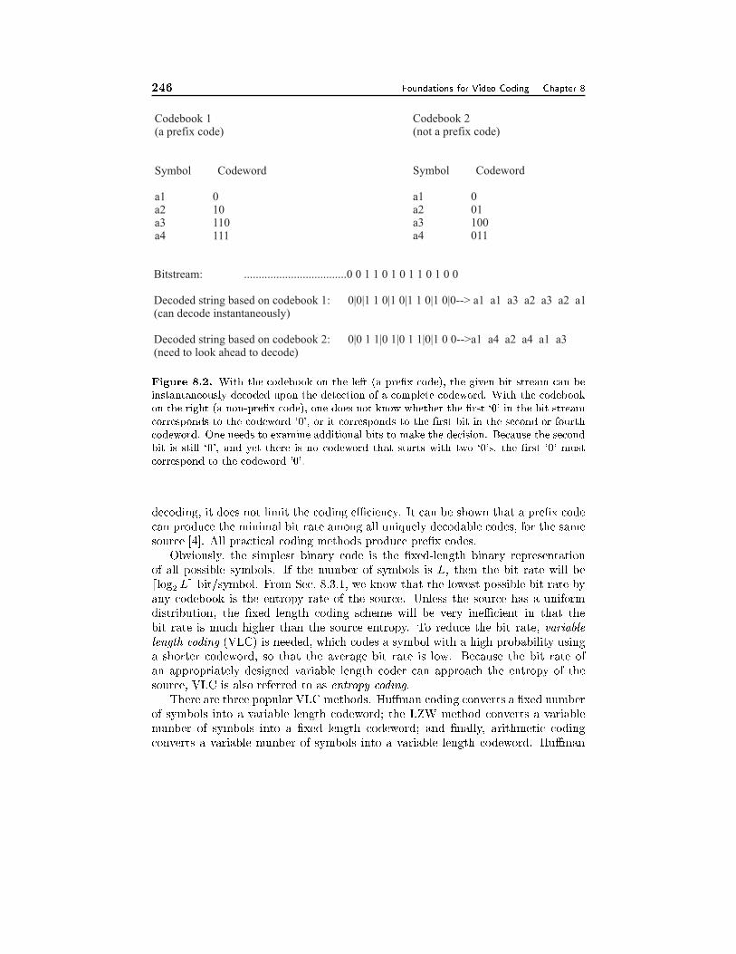
246 Foundations for Video Coding Chapter 8
Codebook 1(a prefix code)
Symbol Codeword
a1 0a2 10a3 110a4 111
Codebook 2(not a prefix code)
Symbol Codeword
a1 0a2 01a3 100a4 011
Bitstream: ...................................0 0 1 1 0 1 0 1 1 0 1 0 0
Decoded string based on codebook 1: a1 a1 a3 a2 a3 a2 a1(can decode instantaneously)
Decoded string based on codebook 2: 0|0 1 1|0 1|0 1 1|0|1 0 0-->a1 a4 a2 a4 a1 a3(need to look ahead to decode)
0|0|1 1 0|1 0|1 1 0|1 0|0-->
Figure 8.2. With the codebook on the left (a pre�x code), the given bit stream can be
instantaneously decoded upon the detection of a complete codeword. With the codebook
on the right (a non-pre�x code), one does not know whether the �rst `0' in the bit stream
corresponds to the codeword `0', or it corresponds to the �rst bit in the second or fourth
codeword. One needs to examine additional bits to make the decision. Because the second
bit is still `0', and yet there is no codeword that starts with two `0's, the �rst `0' must
correspond to the codeword '0'.
decoding, it does not limit the coding eÆciency. It can be shown that a pre�x code
can produce the minimal bit rate among all uniquely decodable codes, for the same
source [4]. All practical coding methods produce pre�x codes.
Obviously, the simplest binary code is the �xed-length binary representation
of all possible symbols. If the number of symbols is L, then the bit rate will be
dlog2 Le bit/symbol. From Sec. 8.3.1, we know that the lowest possible bit rate by
any codebook is the entropy rate of the source. Unless the source has a uniform
distribution, the �xed length coding scheme will be very ineÆcient in that the
bit rate is much higher than the source entropy. To reduce the bit rate, variable
length coding (VLC) is needed, which codes a symbol with a high probability using
a shorter codeword, so that the average bit rate is low. Because the bit rate of
an appropriately designed variable length coder can approach the entropy of the
source, VLC is also referred to as entropy coding.
There are three popular VLC methods. Hu�man coding converts a �xed number
of symbols into a variable length codeword; the LZW method converts a variable
number of symbols into a �xed length codeword; and �nally, arithmetic coding
converts a variable number of symbols into a variable length codeword. Hu�man
Section 8.4. Binary Encoding 247
and arithmetic methods are probability-model-based and both can reach the entropy
bound asymptotically. The arithmetic coding method can more easily achieve the
asymptotic performance and can easily adapt to variations in signal statistics. But
it is also more complex than Hu�man coding. The LZW method [12, 10] does
not require the knowledge of the signal statistics and thus is universally applicable.
But it is less eÆcient than the other two methods. Hu�man and arithmetic coding
methods have been employed in various video coding standards. We describe these
two methods in the following two subsections.
8.4.1 Hu�man Coding
Hu�man coding is the most popular approach for lossless coding of a discrete source
with alphabet A = fa1; a2; : : : ; aLg and pmf p(al). It designs a codebook for all
possible symbols, so that a symbol appearing more frequently is assigned a shorter
codeword. The basic procedure for codebook design using Hu�man coding is as
follows:
Step i: Arrange the symbol probabilities p(al); l = 1; 2; : : : ; L in a decreasing order
and consider them as leaf nodes of a tree.
Step ii: While there is more than one node:
(a) Find the two nodes with the smallest probability and arbitrarily assign
1 and 0 to these two nodes.
(b) merge the two nodes to form a new node whose probability is the sum
of the two merged nodes. Go back to Step i.
Example 8.1 (Scalar Hu�man Coding) An example of Hu�man coding is shown
in Fig. 8.3, in which the source consists of 4 symbols. The symbols and their proba-
bilities are shown on the left two columns. The resulting codewords and the codeword
lengths for these symbols are shown on the right two columns. Also given are the
average bit rate R and the �rst-order entropy of the source H1. We can see that
indeed, H1 < R < H1 + 1:
A notorious disadvantage of Hu�man Coding, when applied to individual sam-
ples, is that at least one bit has to be used for each sample. To further reduce the
bit rate, one can treat each group of N samples as one entity and give each group
a codeword. This leads to Vector Hu�man Coding, a special case of vector lossless
coding. This is shown in the next example.
Example 8.2 (Vector Hu�man Coding) Consider a source with the same al-
phabet and the pmf as in Example 8.1. Suppose we further know that the conditional
distribution of a sample Fn given its previous sample Fn�1 is described by the fol-
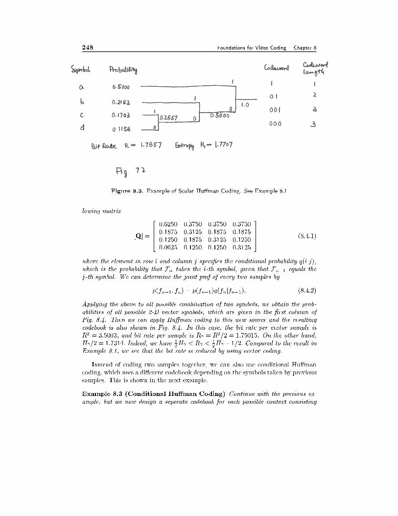
248 Foundations for Video Coding Chapter 8
Figure 8.3. Example of Scalar Hu�man Coding. See Example 8.1
lowing matrix
[Q] =
2664
0:6250 0:3750 0:3750 0:3750
0:1875 0:3125 0:1875 0:1875
0:1250 0:1875 0:3125 0:1250
0:0625 0:1250 0:1250 0:3125
3775 (8.4.1)
where the element in row i and column j speci�es the conditional probability q(ijj),which is the probability that Fn takes the i-th symbol, given that Fn�1 equals the
j-th symbol. We can determine the joint pmf of every two samples by
p(fn�1; fn) = p(fn�1)q(fnjfn�1): (8.4.2)
Applying the above to all possible combination of two symbols, we obtain the prob-
abilities of all possible 2-D vector symbols, which are given in the �rst column of
Fig. 8.4. Then we can apply Hu�man coding to this new source and the resulting
codebook is also shown in Fig. 8.4. In this case, the bit rate per vector sample is
R2 = 3:5003, and bit rate per sample is R2 = R2=2 = 1:75015. On the other hand,
H2=2 = 1:7314: Indeed, we have 12H2 < R2 <
12H2+1=2: Compared to the result in
Example 8.1, we see that the bit rate is reduced by using vector coding.
Instead of coding two samples together, we can also use conditional Hu�man
coding, which uses a di�erent codebook depending on the symbols taken by previous
samples. This is shown in the next example.
Example 8.3 (Conditional Hu�man Coding) Continue with the previous ex-
ample, but we now design a separate codebook for each possible context consisting
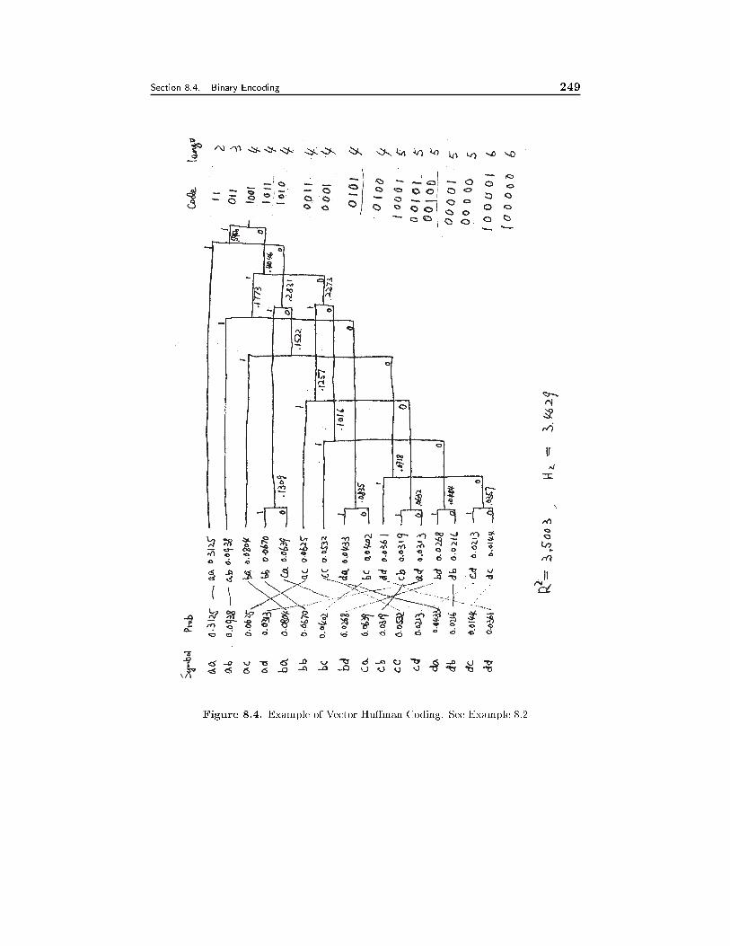
Section 8.4. Binary Encoding 249
Figure 8.4. Example of Vector Hu�man Coding. See Example 8.2
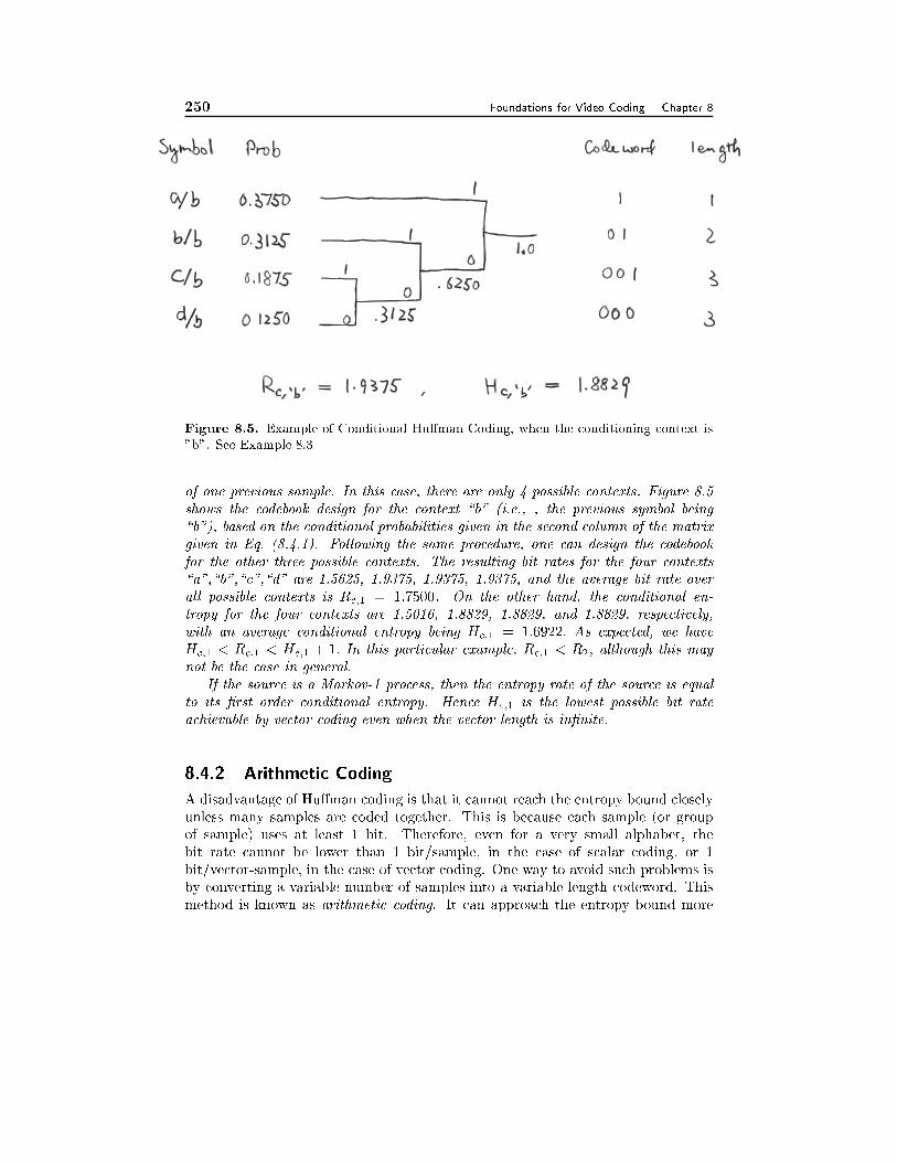
250 Foundations for Video Coding Chapter 8
Figure 8.5. Example of Conditional Hu�man Coding, when the conditioning context is
"b". See Example 8.3
of one previous sample. In this case, there are only 4 possible contexts. Figure 8.5
shows the codebook design for the context \b" (i.e., , the previous symbol being
\b"), based on the conditional probabilities given in the second column of the matrix
given in Eq. (8.4.1). Following the same procedure, one can design the codebook
for the other three possible contexts. The resulting bit rates for the four contexts
\a",\b",\c",\d" are 1.5625, 1.9375, 1.9375, 1.9375, and the average bit rate over
all possible contexts is Rc;1 = 1:7500. On the other hand, the conditional en-
tropy for the four contexts are 1.5016, 1.8829, 1.8829, and 1.8829, respectively,
with an average conditional entropy being Hc;1 = 1:6922: As expected, we have
Hc;1 < Rc;1 < Hc;1 + 1: In this particular example, Rc;1 < R2; although this may
not be the case in general.
If the source is a Markov-1 process, then the entropy rate of the source is equal
to its �rst order conditional entropy. Hence Hc;1 is the lowest possible bit rate
achievable by vector coding even when the vector length is in�nite.
8.4.2 Arithmetic Coding
A disadvantage of Hu�man coding is that it cannot reach the entropy bound closely
unless many samples are coded together. This is because each sample (or group
of sample) uses at least 1 bit. Therefore, even for a very small alphabet, the
bit rate cannot be lower than 1 bit/sample, in the case of scalar coding, or 1
bit/vector-sample, in the case of vector coding. One way to avoid such problems is
by converting a variable number of samples into a variable length codeword. This
method is known as arithmetic coding. It can approach the entropy bound more
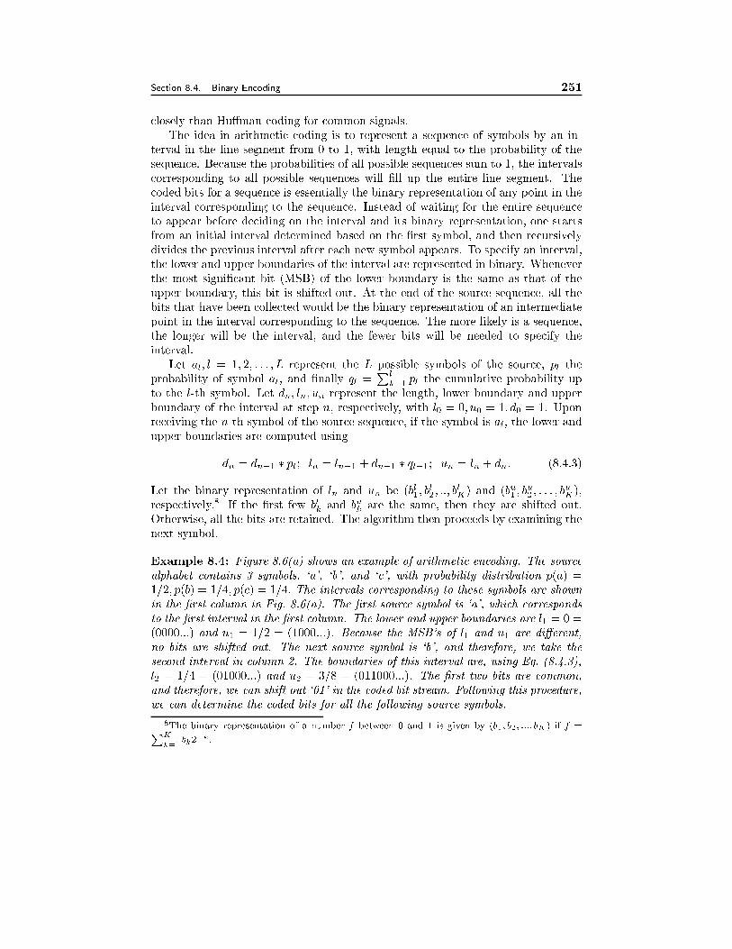
Section 8.4. Binary Encoding 251
closely than Hu�man coding for common signals.
The idea in arithmetic coding is to represent a sequence of symbols by an in-
terval in the line segment from 0 to 1, with length equal to the probability of the
sequence. Because the probabilities of all possible sequences sum to 1, the intervals
corresponding to all possible sequences will �ll up the entire line segment. The
coded bits for a sequence is essentially the binary representation of any point in the
interval corresponding to the sequence. Instead of waiting for the entire sequence
to appear before deciding on the interval and its binary representation, one starts
from an initial interval determined based on the �rst symbol, and then recursively
divides the previous interval after each new symbol appears. To specify an interval,
the lower and upper boundaries of the interval are represented in binary. Whenever
the most signi�cant bit (MSB) of the lower boundary is the same as that of the
upper boundary, this bit is shifted out. At the end of the source sequence, all the
bits that have been collected would be the binary representation of an intermediate
point in the interval corresponding to the sequence. The more likely is a sequence,
the longer will be the interval, and the fewer bits will be needed to specify the
interval.
Let al; l = 1; 2; : : : ; L represent the L possible symbols of the source, pl the
probability of symbol al, and �nally ql =P
l
k=1 pl the cumulative probability up
to the l-th symbol. Let dn; ln; un represent the length, lower boundary and upper
boundary of the interval at step n, respectively, with l0 = 0; u0 = 1; d0 = 1. Upon
receiving the n-th symbol of the source sequence, if the symbol is al, the lower and
upper boundaries are computed using
dn = dn�1 � pl; ln = ln�1 + dn�1 � ql�1; un = ln + dn: (8.4.3)
Let the binary representation of ln and un be (bl1; bl2; ::; b
l
K) and (bu1 ; b
u2 ; : : : ; b
u
K),
respectively.8 If the �rst few blkand bu
kare the same, then they are shifted out.
Otherwise, all the bits are retained. The algorithm then proceeds by examining the
next symbol.
Example 8.4: Figure 8.6(a) shows an example of arithmetic encoding. The source
alphabet contains 3 symbols, `a', `b', and `c', with probability distribution p(a) =
1=2; p(b) = 1=4; p(c) = 1=4: The intervals corresponding to these symbols are shown
in the �rst column in Fig. 8.6(a). The �rst source symbol is `a', which corresponds
to the �rst interval in the �rst column. The lower and upper boundaries are l1 = 0 =
(0000:::) and u1 = 1=2 = (1000:::). Because the MSB's of l1 and u1 are di�erent,
no bits are shifted out. The next source symbol is `b', and therefore, we take the
second interval in column 2. The boundaries of this interval are, using Eq. (8.4.3),
l2 = 1=4 = (01000:::) and u2 = 3=8 = (011000:::). The �rst two bits are common,
and therefore, we can shift out `01' in the coded bit stream. Following this procedure,
we can determine the coded bits for all the following source symbols.
8The binary representation of a number f between 0 and 1 is given by (b1; b2; :::; bK) if f =PK
k=1bk2
�k.
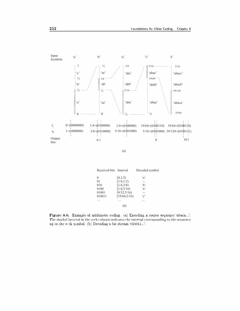
252 Foundations for Video Coding Chapter 8
0
½
1 3/8
‘a’
‘b’
InputSymbols
‘a’ ‘b’ ‘a’ ‘c’
¾
‘c’
‘a’
0
½
¼
3/8
¼
5/16
¼
5/16
19/64
19/64
39/128
5/16
ln
un
0=(0000000)
1=(1000000)
1/4=(0100000)
3/8=(0110000)
1/4=(0100000)
5/16=(0101000)
19/64=(0100110)
5/16=(0101000)
19/64=(0100110)
39/128=(0100111)
Outputbits
0 1 0 011
(a)
Received bits Interval Decoded symbol
0 [0,1/2) ‘a’01 [1/4,1/2) --010 [1/4,3/8) ‘b’0100 [1/4,5/16) ‘a’01001 [9/32,5/16) --010011 [19/64,5/16) ‘c’… … ...
(b)
‘aa’
‘ab’
‘ac’
‘aba’
‘abb’
‘abc’
‘abaa’
‘abab’
‘abac’
‘abaca’
‘abacb’
‘abacc’
Figure 8.6. Example of arithmetic coding. (a) Encoding a source sequence `abaca...'.
The shaded interval in the n-th column indicates the interval corresponding to the sequence
up to the n-th symbol. (b) Decoding a bit stream `010011...'.
Section 8.4. Binary Encoding 253
To decode a received bit stream, one determines the lower and upper boundaries
of an interval corresponding to the received bits. If the interval falls in a range that
can only be associated with a particular source symbol, that symbol is decoded. If
not, additional bits are examined.
Example 8.5: The decoding process for the previous example is shown in Fig. 8.6(b).
The �rst received bit is '0', and the possible lower and upper boundaries both with
`0' as the MSB are l = (0000:::) = 0 and u = (0111:::) = (1000:::) = 1=2. From
the �rst column in Fig. 8.6(a), this interval corresponds to `a', therefore, one can
output `a' as a decoded symbol. With the next received bit `1', the possible lower
and upper boundaries both with `01' as the �rst two bits are l = (0100:::) = 1=4
and u = (0111:::) = (1000:::) = 1=2. From the second column in Fig. 8.6(a), the
range (1=4; 1=2) can come from either `ab' or `ac'. Therefore, one cannot decode
a symbol at this step. With the third bit `0', the lower and upper boundaries are
l = (010000:::) = 1=4 and u = (010111:::) = (011000:::) = 3=8. From the second
column in Fig. 8.6(a), this interval corresponds to `ab'. Therefore, one can output
`b' in this step. Continuing this process, one can decode all the symbols for the given
bit stream.
The above description of arithmetic coding is on a conceptual level only, which
assumes in�nite precision in calculation of the interval boundaries. As more source
symbols are processed, the interval corresponding to the input sequence becomes
increasingly small. To process a reasonably long sequence, one would need a com-
puter with an extremely high precision to specify the boundary values. Fortunately,
it is not necessary to record the absolute boundary values for the encoding and de-
coding process to work. A previously determined interval can be re-scaled to length
1 once a common bit of the lower and upper boundaries is shifted out. Such type
of implementation is known as �nite precision arithmetic coding. Instead of using
fractional arithmetic for the lower and upper bound calculation, integer implemen-
tation, which is simpler, has also been developed. A full description of practical
encoding and decoding algorithms is beyond the scope of this book. The reader is
referred to the excellent tutorial by Witten et al. [11]. A good coverage of both
Hu�man and arithmetic coding can also be found in the book by Sayood [9].
The bit rate of arithmetic coding is bounded by [9]
HN (F)=N � R � HN (F)=N + 2=N; (8.4.4)
where N is the number of symbols in the sequence being coded, HN (F) is the N-th
order entropy of the sequence. Recall that if we code the entire length N sequence
using vector Hu�man coding, the bit rate will be bounded as in Eq. (8.3.4). There-
fore, both methods can approach the entropy bound closely when N is suÆciently
large. However, with Hu�man coding, one must design and store the codebook
for all possible sequences of length N , which has complexity that grows exponen-
tially with N . This limits the sequence length that can be used in practice. With
arithmetic coding, no codebook needs to be designed in advance for each possible
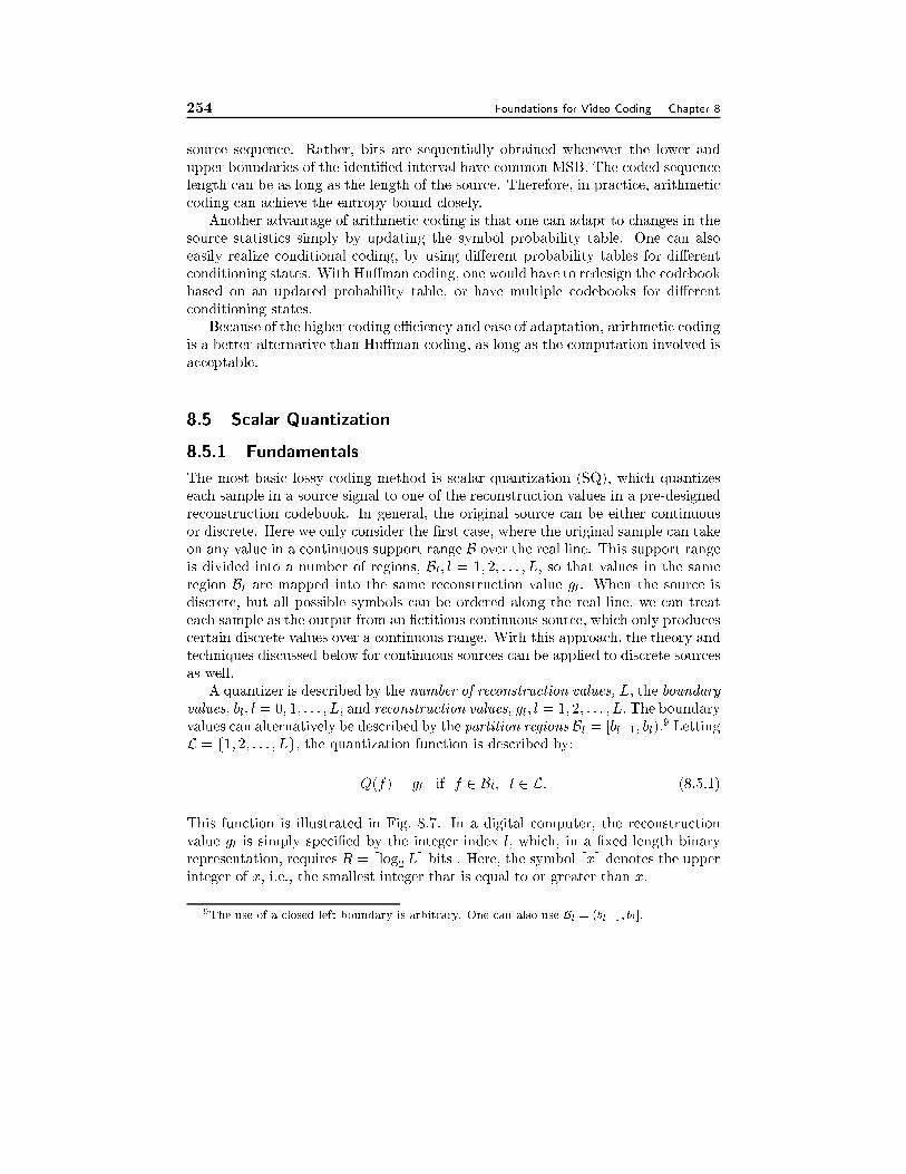
254 Foundations for Video Coding Chapter 8
source sequence. Rather, bits are sequentially obtained whenever the lower and
upper boundaries of the identi�ed interval have common MSB. The coded sequence
length can be as long as the length of the source. Therefore, in practice, arithmetic
coding can achieve the entropy bound closely.
Another advantage of arithmetic coding is that one can adapt to changes in the
source statistics simply by updating the symbol probability table. One can also
easily realize conditional coding, by using di�erent probability tables for di�erent
conditioning states. With Hu�man coding, one would have to redesign the codebook
based on an updated probability table, or have multiple codebooks for di�erent
conditioning states.
Because of the higher coding eÆciency and ease of adaptation, arithmetic coding
is a better alternative than Hu�man coding, as long as the computation involved is
acceptable.
8.5 Scalar Quantization
8.5.1 Fundamentals
The most basic lossy coding method is scalar quantization (SQ), which quantizes
each sample in a source signal to one of the reconstruction values in a pre-designed
reconstruction codebook. In general, the original source can be either continuous
or discrete. Here we only consider the �rst case, where the original sample can take
on any value in a continuous support range B over the real line. This support range
is divided into a number of regions, Bl; l = 1; 2; : : : ; L, so that values in the same
region Bl are mapped into the same reconstruction value gl. When the source is
discrete, but all possible symbols can be ordered along the real line, we can treat
each sample as the output from an �ctitious continuous source, which only produces
certain discrete values over a continuous range. With this approach, the theory and
techniques discussed below for continuous sources can be applied to discrete sources
as well.
A quantizer is described by the number of reconstruction values, L, the boundary
values, bl; l = 0; 1; : : : ; L; and reconstruction values, gl; l = 1; 2; : : : ; L: The boundary
values can alternatively be described by the partition regions Bl = [bl�1; bl):9 Letting
L = f1; 2; : : : ; Lg; the quantization function is described by:
Q(f) = gl if f 2 Bl; l 2 L: (8.5.1)
This function is illustrated in Fig. 8.7. In a digital computer, the reconstruction
value gl is simply speci�ed by the integer index l, which, in a �xed length binary
representation, requires R = dlog2 Le bits . Here, the symbol dxe denotes the upperinteger of x, i.e., the smallest integer that is equal to or greater than x.
9The use of a closed left boundary is arbitrary. One can also use Bl = (bl�1; bl]:
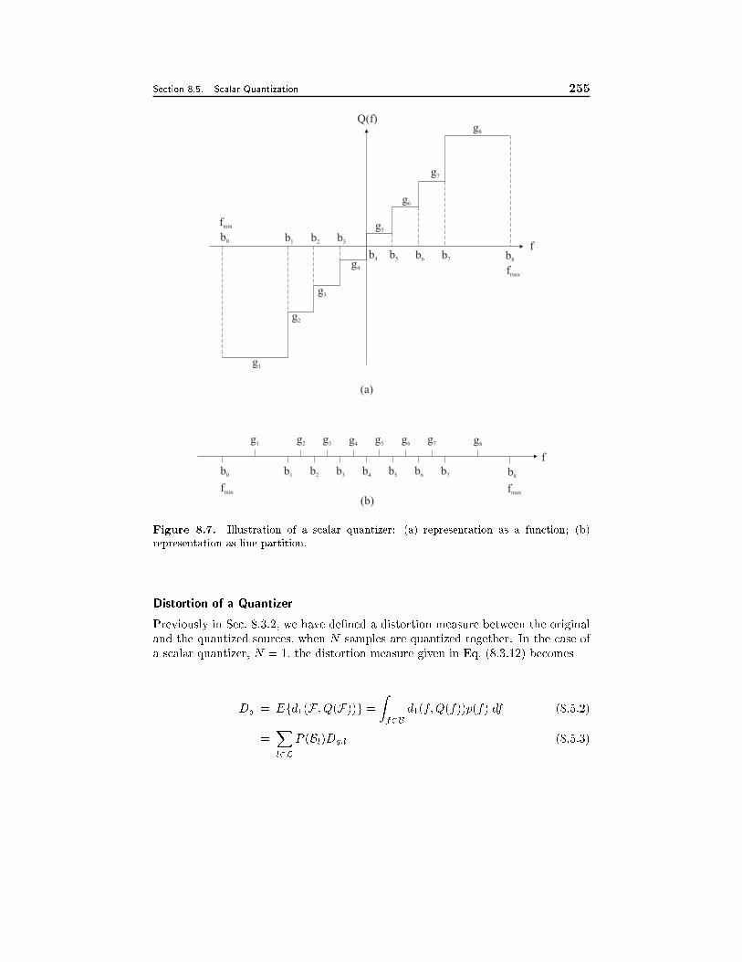
Section 8.5. Scalar Quantization 255
b0
b0
b1
b1
g1
b2
b2
g2
b3
b3
g3
b4
b4
g4
b5
b5
g5
b6
b6
g6
b7
b7
g7 g8
b8
b8
g8
g1
g2
g3
g4
g5
g6
g7
Q(f)
f
f
fmin
fmin
fmax
fmax
(a)
(b)
Figure 8.7. Illustration of a scalar quantizer: (a) representation as a function; (b)
representation as line partition.
Distortion of a Quantizer
Previously in Sec. 8.3.2, we have de�ned a distortion measure between the original
and the quantized sources, when N samples are quantized together. In the case of
a scalar quantizer, N = 1, the distortion measure given in Eq. (8.3.12) becomes
Dq = Efd1(F ; Q(F))g =Zf2B
d1(f;Q(f))p(f) df (8.5.2)
=Xl2L
P (Bl)Dq;l (8.5.3)
256 Foundations for Video Coding Chapter 8
with
Dq;l =
Zf2Bl
d1(f; gl)p(f jf 2 Bl) df: (8.5.4)
In the above equations, F represents the RV corresponding to any sample in a
source F , p(f); f 2 B; the pdf of F , P (Bl) =RBlp(f)df the probability that f 2 Bl,
and p(f jf 2 Bl) = p(f)=P (Bl) the conditional pdf of F given F 2 Bl: Obviously,Dq;l denotes the mean distortion incurred in region Bl:
When d1(f; g) = (f � g)2, the above distortion reduces to the MSE, which is
equal to the variance of the quantization errorF�Q(F), denoted by �2q : Speci�cally,
�2q = EfjF �Q(F)j2g =Xl2L
P (Bl)Z bl
bl�1
(f � gl)2p(f jBl) df: (8.5.5)
8.5.2 Uniform Quantization
The simplest scalar quantizer is a uniform quantizer, which has equal distances
between adjacent boundary values and between adjacent reconstruction values:
bl � bl�1 = gl � gl�1 = q (8.5.6)
where q is called the quantization stepsize. Such a quantizer is only applicable to a
signal with a �nite dynamic range B. Let fmin and fmax represent the minimal and
maximal values, then B = fmax � fmin. The quantizer is speci�ed by the number
of quantization levels L, or the bit rate R, or the quantization stepsize q. These
parameters are related by q = B=L = B2�R: The boundary and reconstruction
values are given by
bl = l � q + fmin; gl = (l � 1) � q + q=2 + fmin: (8.5.7)
The quantization function can be described in a closed form:
Q(f) = bf � fmin
qc � q + q
2+ fmin: (8.5.8)
In the above, bxc represents the oor function of x, i.e., the largest integer that is
equal or smaller than x: See Fig. 8.8.
If the source is uniformly distributed, i.e.,
p(f) =
�1=B f 2 (fmin; fmax)
0 otherwise(8.5.9)
then substituting Eqs. (8.5.7) and (8.5.9) into Eq. (8.5.5) yields
�2q =q2
12= �2f 2
�2R (8.5.10)

Section 8.5. Scalar Quantization 257
b0
fminfmax
b1 b2 b3 b4 b5 b6 b7 b8
g8
g1
g2
g3
g4
g5
g6
g7
Q(f)
f
q
Figure 8.8. A uniform quantizer.
where �2f= B2=12 is the variance of the original signal F . The signal to noise ratio
(SNR) of the quantizer is
SNR = 10 log10�2f
�2q= (20 log10 2) R = 6:02R (dB) (8.5.11)
Therefore, every additional bit in a uniform quantizer leads to a 6.02 dB gain in
SNR for a uniform source. This is a well known result in the quantization theory.
8.5.3 Optimal Scalar Quantizer
The uniform quantizer introduced thus far are simple to implement, but may not
be most eÆcient in representing a source. In this section, we examine how to design
an optimal scalar quantizer, so that the distortion is minimized for a �xed bit rate,
given the source pdf p(f):
Minimal Mean Square Error (MMSE) Quantizer
In such a quantizer, bl; gl are chosen such that the MSE �2q is minimized for a
given L. From the calculus of variations, the necessary conditions are@�
2q
@bl= 0 and
258 Foundations for Video Coding Chapter 8
@�2q
@gl= 0;8l: From (8.5.5),
@�2q
@bl=
@
@bl
Zbl
bl�1
(f � gl)2p(f) df +
Zbl+1
bl
(f � gl+1)2p(f) df
!
= (bl � gl)2p(bl)� (bl � gl+1)
2p(bl) = 0;
@�2q
@gl=
@
@gl
Z bl
bl�1
(f � gl)2p(f) df = �
Z bl
bl�1
2(f � gl)p(f) df = 0:
Simpli�cation of the preceding equations yields:
bl =gl + gl+1
2; (8.5.12)
gl = EfFjF 2 Blg =ZBl
f p(f jf 2 Bl) df: (8.5.13)
The conditional mean EfFjF 2 Blg is referred to as the centroid of Bl:The results in Eqs. (8.5.12) and (8.5.13) state that the optimum boundary values
lie halfway between the optimal reconstruction values, which, in turn, lie at the
centroids of the regions between the boundary values. Note that requiring bl =
(gl + gl+1)=2 is equivalent to quantizing any f 2 (gl; gl+1) to gl if f is closer to
gl than gl+1. A more general statement is that any value f is quantized to the
reconstruction value that is closest to f . Therefore, Eq. (8.5.12) can be equivalently
written as
Bl = ff : d1(f; gl) � d1(f; g0l);8l0 6= lg: (8.5.14)
The condition given by Eq. (8.5.12) or Eq. (8.5.14) is called the nearest neighbor
condition. On the other hand, equation (8.5.13) is known as the centroid condition.
It can be shown that the nearest neighbor condition given in Eq. (8.5.14) is still
valid with a distortion measure rather than the MSE. The centroid condition in
Eq. (8.5.13) however has to be changed to
gl = argmingfEfd1(F ; g)jF 2 Blgg; (8.5.15)
where argmingfE(g)g represents the argument g that minimizes the function E(g).
The gl de�ned in Eq. (8.5.15) is called the generalized centroid of Bl, and its solutiondepends on the de�nition of d1(f; g). For example, if d1(f; g) = jf � gj, then gl is
the median value in Bl: See Prob. 8.12.An important property of a MMSE quantizer is that it equalizes the quantization
error in di�erent partition regions, i.e.,
P (Bl)Dg;l = Dq ;8l 2 L (8.5.16)
For other important statistical properties of an optimal quantizer, see [5, 4]. Also,
see Prob. 8.8.
Section 8.5. Scalar Quantization 259
MMSE Quantizer for a Uniform Source
Substituting the uniform distribution in Eq. (8.5.9) into Eqs. (8.5.12) and (8.5.13)
will yield the solution given in Eq. (8.5.7). Thus, as expected, the MMSE quantizer
for a uniform source is uniform.
MMSE Quantizer for a Non-Uniform Source
For an arbitrary pdf p(f), the conditions in Eqs. (8.5.12) and (8.5.13) do not always
have a closed-form solution. Numerical procedures need to be used to determine
the optimal set of bl; gl. Table 4.3 in [5] gives the optimal ~bl and ~gl for uniform,
Gaussian, Laplacian, and Gamma sources with unit variance and zero mean. It can
be shown (Prob. 8.10) that the optimal bl and gl for a source with arbitrary mean
�f and variance �2fcan be obtained by:
bl = �f~bl + �f ; gl = �f ~gl + �f : (8.5.17)
The MMSE quantizer for a non-uniform source is in general non-uniform, i.e.,
the partition regions are not equal in length. In this case, the quantized value
cannot be determined by a closed-form formula as with a uniform quantizer. In
general, one must compare the given value f with all boundary values, until the
region for which bl�1 � f < bl is found. Alternatively, one can �nd gl that is closest
to f . A sequential search would require up to L comparisons. Using a binary tree
search procedure, the number of comparisons can be reduced to dlog2 Le:
Asymptotic Performance of MMSE Quantizer
For a source with an arbitrary pdf, it is diÆcult to derive a closed-form solution for
the quantizer parameters bl; gl and consequently the quantization error �2q , using
the nearest neighbor condition and the centroid condition. However, when the bit
rate R and consequently the quantization level L = 2R is very high, a closed form
solution for the MMSE quantizer in terms of the pdf can be derived [5, 4]. The
associated quantization error can be expressed as
�2q = �2�2f2�2R (8.5.18)
with
�2 =1
12
�Z 1
�1
~p(f)1=3df
�3
; (8.5.19)
where ~p(f) = �fp(�ff) denotes the pdf of a normalized source with unit variance.
Comparing the above with Eq. (8.5.10), we see that �2 = 1 for a uniform source.
For a non-uniform source, �2 > 1 in general. In particular, for a Gaussian source,
�2 = 2:71: Recall that the distortion-rate bound for an i.i.d Gaussian source is given
in Eq. (8.3.20). Therefore, using the best scalar quantizer is still o� from the bound
by 12log2 �
2=0.7191 bit/sample. For the values of �2 for several other sources, see [5,
260 Foundations for Video Coding Chapter 8
Table 4.8]. To be closer to the bound, multiple samples must be quantized together.
The factor �2 can be reduced by applying variable length coding to the quantized
indices. This is discussed further in Sec. 8.6.4.
Llyod Algorithm for MMSE Quantizer Design Based on Training Data
When the distribution of the signal to be quantized is unknown, the quantizer can
be designed based on a training set containing representative samples to be quan-
tized. A popular method for designing a quantizer based on the training data is
the Lloyd algorithm [7, 4]. As shown in Fig. 8.9, the algorithm updates the recon-
struction and boundary values iteratively. At each iteration, one �rst recalculates
the reconstruction values based on the centroid condition, and then partition all
the training samples based on the nearest neighbor condition. The statistical ex-
pectation required in the calculation of the generalized centroid and distortion are
approximated by sample averages. Under the MSE criterion, the reconstruction
value for a partition is simply the mean value of training samples belonging to
that partition, whereas the boundary values are simply the average of two adjacent
reconstruction values.
8.6 Vector Quantization
8.6.1 Fundamentals
Rather than quantizing one sample at a time, one can quantize a group ofN samples
together. Each sample group is known as a vector, and the process of quantizing
a vector at a time is called vector quantization (VQ). In the image or video case,
a vector usually corresponds to a square block of pixels. The motivation for using
vector quantization (VQ) primarily stems from the observation that in a typical
image or video frame, samples in a block are correlated so that there are certain
block patterns that are more likely than others. The task of VQ is essentially
to �nd the L most popular patterns, and replace any given block by one of the
representative patterns that resembles the original pattern closest.
The above discussion assumes that a vector corresponds to a group of sample
values. In a source in which each sample is described by multiple values, each
sample can itself be quantized using a vector quantizer. For example, each sample
in a color image contains three components. To display a 24 bit color image on a
computer monitor using an 8 bit graphics card, one has to �nd 256 colors that best
represent all possible 224 = 16 million colors.
Consider each possibleN -D vector f as a point in anN -D space, the VQ problem
is to partition the N -D space into L regions Bl, and representing all the points in
region Bl by a representative point gl. This process is illustrated in Fig. 8.10 for the
case of N = 2: We call Bl the partition regions and gl the reconstruction vectors
or codewords. The set containing all codewords fgl; l 2 Lg is called the codebook.10
10Note that each reconstruction codeword needs to be mapped into a binary codeword, to
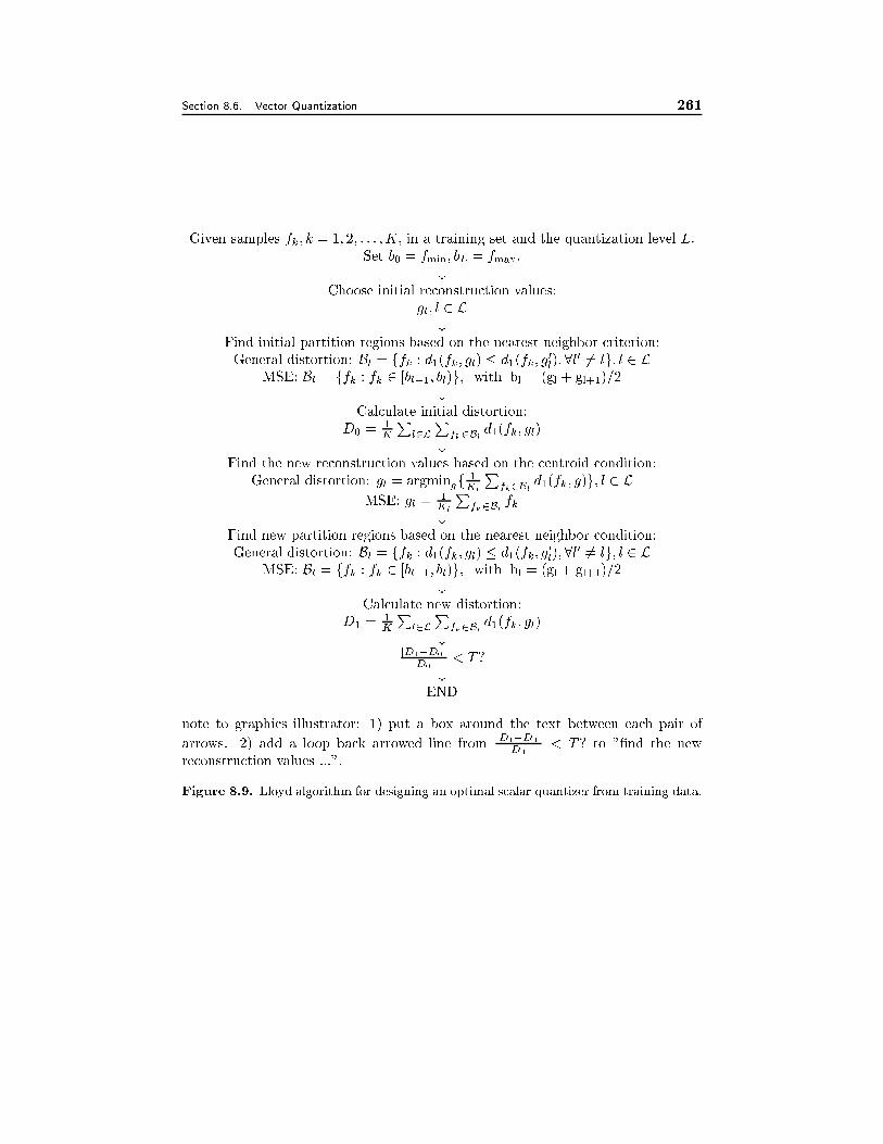
Section 8.6. Vector Quantization 261
Given samples fk; k = 1; 2; : : : ;K; in a training set and the quantization level L.
Set b0 = fmin; bL = fmax:
#Choose initial reconstruction values:
gl; l 2 L#
Find initial partition regions based on the nearest neighbor criterion:
General distortion: Bl = ffk : d1(fk; gl) � d1(fk; g0l);8l0 6= lg; l 2 L
MSE: Bl = ffk : fk 2 [bl�1; bl)g; with bl = (gl + gl+1)=2
#Calculate initial distortion:
D0 =1K
Pl2L
Pfk2Bl
d1(fk; gl)
#Find the new reconstruction values based on the centroid condition:
General distortion: gl = argmingf 1Kl
Pfk2Bl
d1(fk; g)g; l 2 LMSE: gl =
1Kl
Pfk2Bl
fk#
Find new partition regions based on the nearest neighbor condition:
General distortion: Bl = ffk : d1(fk; gl) � d1(fk; g0l);8l0 6= lg; l 2 L
MSE: Bl = ffk : fk 2 [bl�1; bl)g; with bl = (gl + gl+1)=2
#Calculate new distortion:
D1 =1K
Pl2L
Pfk2Bl
d1(fk; gl)
#jD1�D0j
D0< T ?
#END
note to graphics illustrator: 1) put a box around the text between each pair of
arrows. 2) add a loop back arrowed line fromjD1�D0j
D0< T ? to "�nd the new
reconstruction values ...".
Figure 8.9. Lloyd algorithm for designing an optimal scalar quantizer from training data.
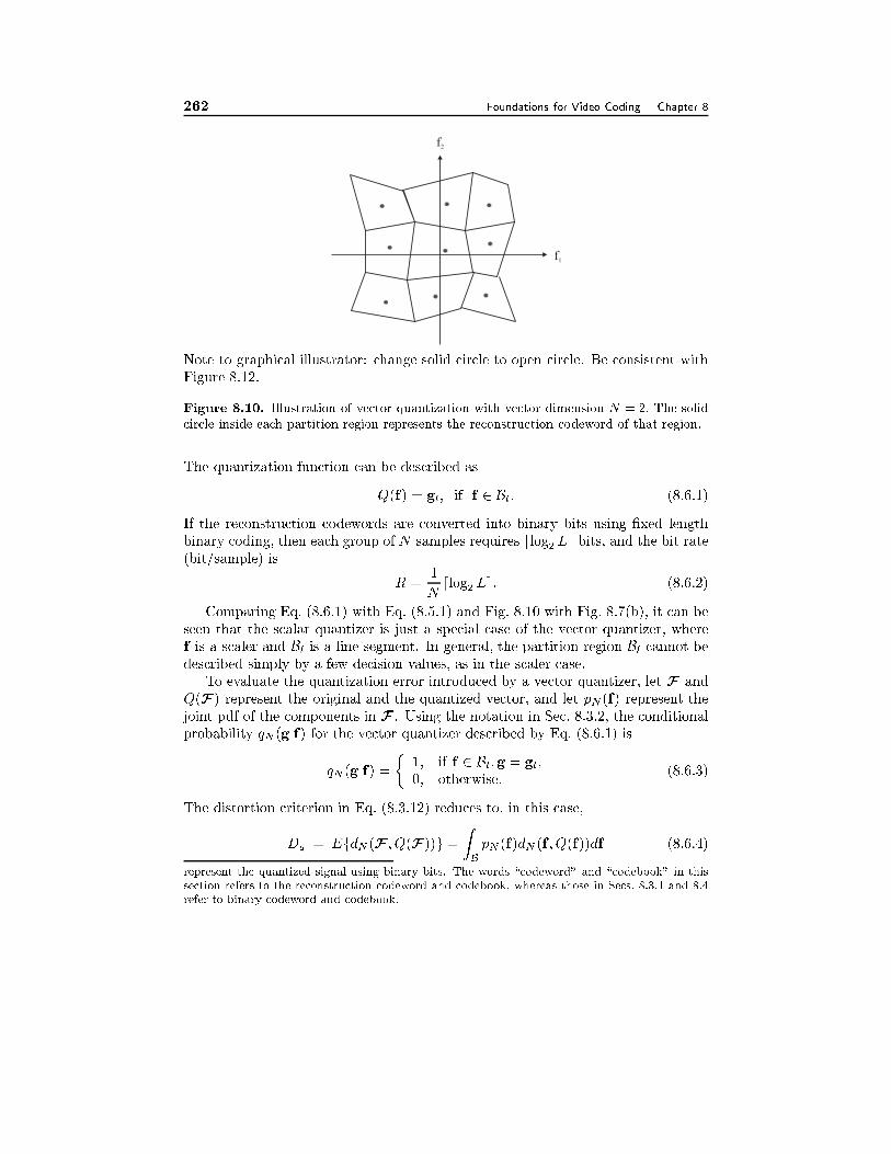
262 Foundations for Video Coding Chapter 8
f1
f2
Note to graphical illustrator: change solid circle to open circle. Be consistent with
Figure 8.12.
Figure 8.10. Illustration of vector quantization with vector dimension N = 2: The solid
circle inside each partition region represents the reconstruction codeword of that region.
The quantization function can be described as
Q(f) = gl; if f 2 Bl: (8.6.1)
If the reconstruction codewords are converted into binary bits using �xed length
binary coding, then each group of N samples requires dlog2 Le bits, and the bit rate
(bit/sample) is
R =1
Ndlog2 Le: (8.6.2)
Comparing Eq. (8.6.1) with Eq. (8.5.1) and Fig. 8.10 with Fig. 8.7(b), it can be
seen that the scalar quantizer is just a special case of the vector quantizer, where
f is a scaler and Bl is a line segment. In general, the partition region Bl cannot bedescribed simply by a few decision values, as in the scaler case.
To evaluate the quantization error introduced by a vector quantizer, let F and
Q(F) represent the original and the quantized vector, and let pN (f) represent the
joint pdf of the components in F . Using the notation in Sec. 8.3.2, the conditional
probability qN (gjf) for the vector quantizer described by Eq. (8.6.1) is
qN (gjf) =�
1; if f 2 Bl;g = gl;
0; otherwise:(8.6.3)
The distortion criterion in Eq. (8.3.12) reduces to, in this case,
Dq = EfdN (F ; Q(F))g =ZB
pN (f)dN (f ; Q(f))df (8.6.4)
represent the quantized signal using binary bits. The words \codeword" and \codebook" in this
section refers to the reconstruction codeword and codebook, whereas those in Secs. 8.3.1 and 8.4
refer to binary codeword and codebook.
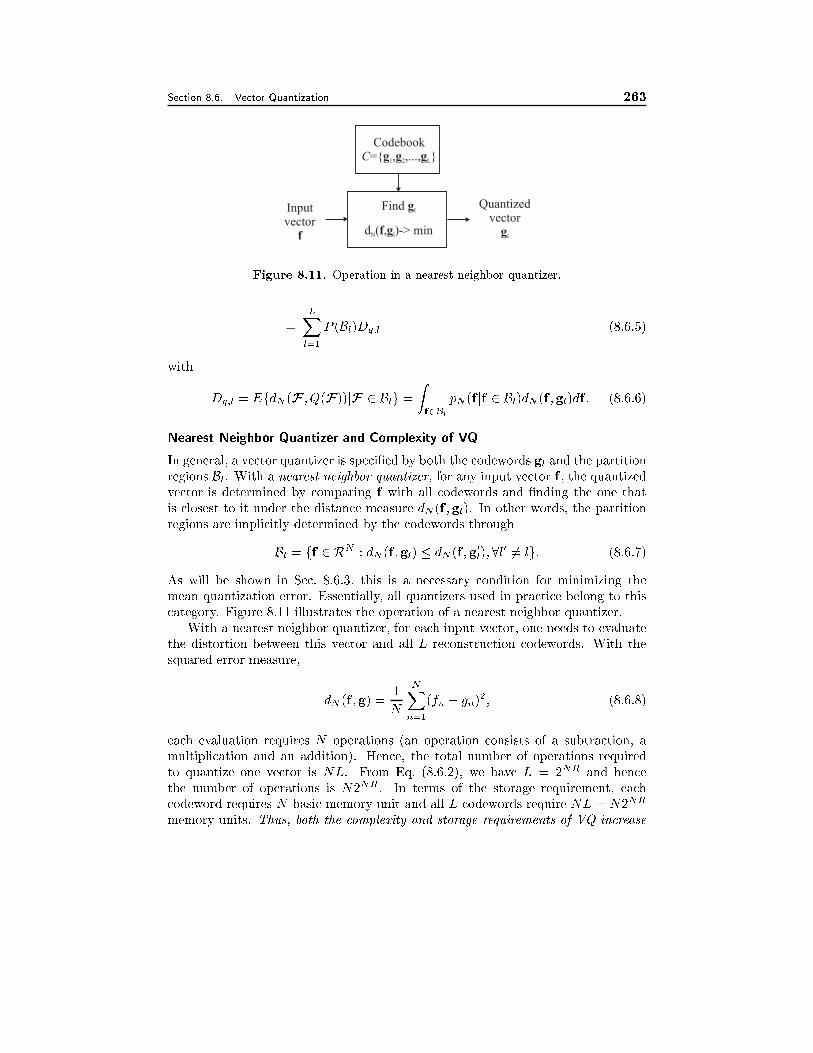
Section 8.6. Vector Quantization 263
Codebook={ , ,..., }C g g g1 2 L
Find
d ( , )-> minN lf g
glQuantized
vectorgl
Inputvector
f
Figure 8.11. Operation in a nearest neighbor quantizer.
=
LXl=1
P (Bl)Dq;l (8.6.5)
with
Dq;l = EfdN (F ; Q(F))jF 2 Blg =Zf2Bl
pN(f jf 2 Bl)dN (f ;gl)df : (8.6.6)
Nearest Neighbor Quantizer and Complexity of VQ
In general, a vector quantizer is speci�ed by both the codewords gl and the partition
regions Bl. With a nearest neighbor quantizer, for any input vector f , the quantized
vector is determined by comparing f with all codewords and �nding the one that
is closest to it under the distance measure dN (f ;gl). In other words, the partition
regions are implicitly determined by the codewords through
Bl = ff 2 RN : dN (f ;gl) � dN (f ;g0l);8l0 6= lg: (8.6.7)
As will be shown in Sec. 8.6.3, this is a necessary condition for minimizing the
mean quantization error. Essentially, all quantizers used in practice belong to this
category. Figure 8.11 illustrates the operation of a nearest neighbor quantizer.
With a nearest neighbor quantizer, for each input vector, one needs to evaluate
the distortion between this vector and all L reconstruction codewords. With the
squared error measure,
dN (f ;g) =1
N
NXn=1
(fn � gn)2; (8.6.8)
each evaluation requires N operations (an operation consists of a subtraction, a
multiplication and an addition). Hence, the total number of operations required
to quantize one vector is NL. From Eq. (8.6.2), we have L = 2NR and hence
the number of operations is N2NR. In terms of the storage requirement, each
codeword requires N basic memory unit and all L codewords require NL = N2NR
memory units. Thus, both the complexity and storage requirements of VQ increase
264 Foundations for Video Coding Chapter 8
exponentially with the vector dimension N . Recall that Theorem 8.4 tells us that
the RD bound for a source is usually achieved only when N reaches in�nity. In
general, the larger is N , the more eÆcient is the coder. However, the exponential
growth of the complexity with N limits the vector dimension that can be used
in practice. Consider the quantization of video frames, by which each block of
N pixels are quantized using a size L codebook. Assuming the frame rate is ftand the frame size is Nx � Ny, then the number of operations per second will be
(ftNxNy=N) � N2NR = ftNxNy2NR: For a CCIR 601 video Y-component, ft =
30; Nx = 720; Ny = 480, a vector size of 4 � 4 and bit rate of 1 bit/sample lead
to an operation count of 6:8E + 11 per second! For image and video coding, N is
usually limited to 4� 4 or below.
To reduce the complexity, similar to binary search in the SQ case, one does not
have to do exhaustive search if each partition region is a polytope. In this case,
di�erent partition regions are de�ned by intersecting hyperplanes. One can compare
a given vector with one hyperplane at a time, each time eliminating codewords on
one side of the plane. This way, the number of comparisons can be reduced to
a number signi�cantly lower than L, but may not be as low as log2 L, unless the
codebook has a special tree-structure. To further reduce the complexity, various
fast VQ schemes have been developed, which impose certain constraints on the
codebook structure, so that the number of comparisons can be reduced. The book
by Gersho and Gray [4] provides an extensive coverage of various VQ techniques.
8.6.2 Lattice Vector Quantizer
As we have learned in Sec. 8.5.2, the simplest scalar quantizer is a uniform quantizer,
in which a certain range of the real line is partitioned into equal-length quantization
bins. An analog of the uniform quantizer in the VQ case is a lattice quantizer,
in which all the partition regions have the same shape and size, and in fact are
all shifted versions of a basic region, which is the Voronoi region of the lattice.
Figure 8.12 shows two lattice quantizers, using rectangular and hexagonal lattices,
respectively. Previously in Chap. 3, we have introduced the concept of lattice for
uniform sampling over a multi-dimensional space. Here we see that lattices can also
be used to de�ne uniform quantizers over a multi-dimensional space.
Recall that a lattice � in anN -D real spaceRN is de�ned by a set of basis vectors
vn; n = 1; 2; : : : ; N or equivalently a generating matrix [V] = [v1;v2; : : : ;vN ]: The
points in a lattice are those vectors that can be represented as
gl =
NXn=1
ml;nvn = [V]ml; (8.6.9)
where ml;n 2 Z are integers or ml 2 ZN is an N -D integer vector. Usually a
codeword gl is indexed by its corresponding ml. The Voronoi region V of � is the
region in which all points are closer to the origin than any other non-zero lattice
points. With a lattice quantizer, the codebook consists of all points in a lattice,
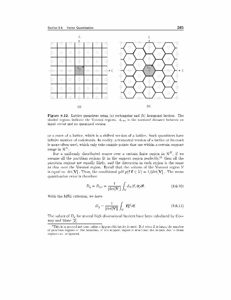
Section 8.6. Vector Quantization 265
(a) (b)
dmaxdmax
f1f1
f2f2
Figure 8.12. Lattice quantizers using (a) rectangular and (b) hexagonal lattices. The
shaded regions indicate the Voronoi regions. dmax is the maximal distance between an
input vector and its quantized version.
or a coset of a lattice, which is a shifted version of a lattice. Such quantizers have
in�nite number of codewords. In reality, a truncated version of a lattice or its coset
is more often used, which only take sample points that are within a certain support
range in RN .
For a uniformly distributed source over a certain �nite region in RN , if we
assume all the partition regions �t in the support region perfectly,11 then all the
partition regions are equally likely, and the distortion in each region is the same
as that over the Voronoi region. Recall that the volume of the Voronoi region Vis equal to jdet[V]j: Thus, the conditional pdf p(f jf 2 V) = 1=jdet[V]j. The mean
quantization error is therefore
Dq = Dq;l =1
jdet[V]jZV
dN (f ;0)df : (8.6.10)
With the MSE criterion, we have
Dq =1
jdet[V]jZV
kfk2df : (8.6.11)
The values of Dq for several high dimensional lattices have been tabulated by Con-
way and Slone [2].
11This is in general not true unless a hypercubic lattice is used. But when L is large, the number
of partition regions on the boundary of the support region is small and the impact due to those
regions can be ignored.
266 Foundations for Video Coding Chapter 8
It is worth noting that even for an i.i.d. source, VQ can improve the coding
eÆciency over SQ. This is because VQ allows more exibility in packing a space
using partition regions. Consider the two examples given in Fig. 8.12. In either
case, the maximum distortion in representing a point in any region by its center
(the codeword) is dmax = 1, so that the two quantizers will yield the same maximum
distortion. But to �ll the same 2-D space, fewer number of hexagons are needed,
because the Voronoi region for the hexagonal lattice is larger than that for the rect-
angular lattice. Speci�cally, the areas of the Voronoi regions for the rectangular
and hexagonal lattices in this example are 2d2max and 2:59d2max, respectively. In the
entire support region considered in the �gure, the rectangular lattice has more than
36 partition regions, whereas the hexagonal lattice has 30 regions.12 Now, the rect-
angular lattice quantizer can also be realized by applying a uniform scalar quantizer
in each dimension. This means that even when two samples are independent and
both are uniformly distributed, quantizing them together as a vector can reduce the
bit rate, with a well-designed vector quantizer.
Implementation of a lattice quantizer As described before, for an arbitrary near-
est neighbor quantizer, the quantization of a given vector involves an exhaustive
search. This is not needed with a lattice quantizer. In this case, one can �rst
determine a real index vector of the quantized vector by
m = [V]�1f : (8.6.12)
Then one can evaluate the distortions associated with all the integer index vectors
neighboring to m, by taking the lower and upper integer of each component of m,
and see which one gives the minimal distortion. For a vector dimension N , at most
2N candidate vectors need to be evaluated. To further reduce the complexity, one
can also simply round m to the nearest integer vector. The reader is referred to [2]
for a more detailed discussion on lattice encoding algorithms and performances.
8.6.3 Optimal Vector Quantizer
Although lattice quantizers are simple to implement, they may not be the most
eÆcient when the source is not uniformly distributed. For a given vector dimension
N and the source pdf pN (f), it is desirable to design an optimal quantizer that
minimizes a given distortion criterion for a �xed bit rate R or equivalently the
codebook size L. Ideally, one needs to determine the codewords gl and the partition
regions Bl simultaneously to minimize the average distortion Dq. The optimal
solution is however diÆcult to �nd. Instead, one can proceed in two stages. First,
for given codewords gl; l 2 L, the partition regions Bl; l 2 L; should be such that theaverage distortion over all regions, Dq, is minimized. Second, for a given partition
region Bl, the codeword gl should be chosen to minimize the distortion within Bl,Dq;l.
12Recall that from Chap. 3, we know that the hexagonal lattice is more eÆcient in covering a
space.
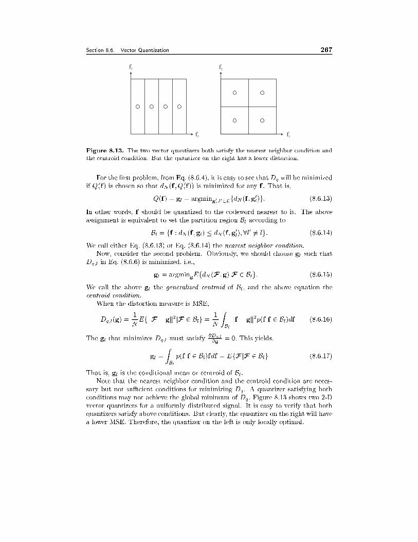
Section 8.6. Vector Quantization 267
f1f1
f2f2
Figure 8.13. The two vector quantizers both satisfy the nearest neighbor condition and
the centroid condition. But the quantizer on the right has a lower distortion.
For the �rst problem, from Eq. (8.6.4), it is easy to see that Dq will be minimized
if Q(f) is chosen so that dN (f ; Q(f)) is minimized for any f . That is,
Q(f) = gl = argming0l;l02LfdN (f ;g0l)g: (8.6.13)
In other words, f should be quantized to the codeword nearest to it. The above
assignment is equivalent to set the partition region Bl according toBl = ff : dN (f ;gl) � dN (f ;g
0l);8l0 6= lg: (8.6.14)
We call either Eq. (8.6.13) or Eq. (8.6.14) the nearest neighbor condition.
Now, consider the second problem. Obviously, we should choose gl such that
Dq;l in Eq. (8.6.6) is minimized, i.e.,
gl = argmingEfdN (F ;g)jF 2 Blg: (8.6.15)
We call the above gl the generalized centroid of Bl; and the above equation the
centroid condition.
When the distortion measure is MSE,
Dq;l(g) =1
NEfkF � gk2jF 2 Blg = 1
N
ZBl
kf � gk2p(f jf 2 Bl)df (8.6.16)
The gl that minimizes Dq;l must satisfy@Dq;l
@g= 0: This yields,
gl =
ZBl
p(f jf 2 Bl)fdf = EfF jF 2 Blg (8.6.17)
That is, gl is the conditional mean or centroid of Bl.Note that the nearest neighbor condition and the centroid condition are neces-
sary but not suÆcient conditions for minimizing Dq . A quantizer satisfying both
conditions may not achieve the global minimum of Dq: Figure 8.13 shows two 2-D
vector quantizers for a uniformly distributed signal. It is easy to verify that both
quantizers satisfy above conditions. But clearly, the quantizer on the right will have
a lower MSE. Therefore, the quantizer on the left is only locally optimal.
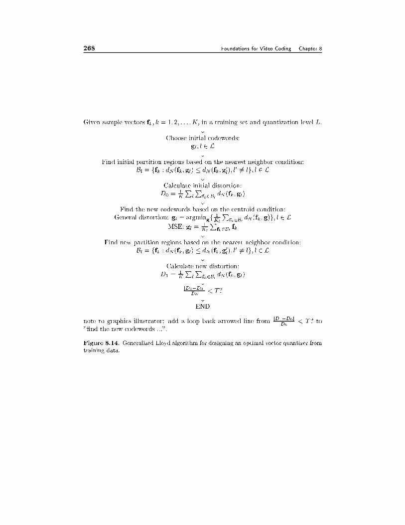
268 Foundations for Video Coding Chapter 8
Given sample vectors fk; k = 1; 2; : : : ;K; in a training set and quantization level L.
#Choose initial codewords:
gl; l 2 L#
Find initial partition regions based on the nearest neighbor condition:
Bl = ffk : dN (fk;gl) � dN (fk;g0l); l0 6= lg; l 2 L
#Calculate initial distortion:
D0 =1K
Pl
Pfk2Bl
dN (fk ;gl)
#Find the new codewords based on the centroid condition:
General distortion: gl = argmingf 1Kl
Pfk2Bl
dN (fk ;g)g; l 2 LMSE: gl =
1Kl
Pfk2Bl
fk#
Find new partition regions based on the nearest neighbor condition:
Bl = ffk : dN (fk;gl) � dN (fk;g0l); l0 6= lg; l 2 L
#Calculate new distortion:
D1 =1K
Pl
Pfk2Bl
dN (fk ;gl)
#jD1�D0j
D0< T ?
#END
note to graphics illustrator: add a loop back arrowed line fromjD1�D0j
D0< T ? to
"�nd the new codewords ...".
Figure 8.14. Generalized Lloyd algorithm for designing an optimal vector quantizer from
training data.
Section 8.6. Vector Quantization 269
Generalized Lloyd Algorithm for Designing Optimal Vector Quantizer
For an arbitrary source, it is diÆcult to derive closed-form solutions for gl;Bl; l 2 L.A locally optimal solution can be obtained by the generalized Lloyd algorithm.13
Like the Lloyd algorithm for SQ, the Generalized Lloyd algorithm for VQ iteratively
determines the optimal gl and Bl based on some training data. Figure 8.14 shows
the ow-chart of this algorithm. Comparing this �gure to Fig. 8.9, one can easily
see the analogy between these two algorithms.
Example 8.6 (Vector Quantizer Design) Figure 8.15 shows an example of quan-
tizer design using the Generalized Lloyd algorithm under the MSE criterion. Within
each iteration, we �rst recalculate the centroid vector (indicated by a circle) for each
previously determined partition region, by averaging all the samples in that region,
and then we repartition (indicated by ovals) all the samples based on their distances
to the newly updated centroid vectors. Results for the �rst 3 iterations are shown.
Because the partition after the 3rd iteration remains the same as that after the 2nd
iteration, the 4th iteration will not change the codewords and consequently the parti-
tion regions. Therefore, the result given after the 3rd iteration is the �nal solution.
The resulting quantizer by the generalized Lloyd algorithm depends on the initial
codewords. When they are not chosen properly, the algorithm may converge to a
bad local minimum that is far from the global one. One simple and yet quite
e�ective way to chose the initial codewords is by using the codewords that would
have resulted from applying uniform scalar quantization in each dimension. For
an extensive coverage of VQ design algorithms, including the selection of initial
codewords, see [4].
8.6.4 Entropy-Constrained Optimal Quantizer Design
Until now, we have assumed that each codeword in a size L codebook takes dlog2 Lebits to represent. Because the reconstruction codewords usually appear with dif-
ferent probabilities, we can further reduce the bit rate by using Hu�man coding or
other variable length lossless coding methods. In the methods described for optimal
quantizer design in Secs. 8.5.3 and 8.6.3, we have tried to minimize the distortion for
a given bit rate R or codebook size L, by assuming R is related to L by Eq. (8.6.2).
The resulting solutions in terms of gl;Bl are not optimal any more, if the quantized
vectors are coded using variable length coding. With entropy-constrained optimal
quantizer design, we minimize the distortion subject to a rate constraint where the
rate is assumed to be equal to the entropy of the quantized source. If we code one
codeword at a time, then the bit rate is bounded by
�RN = � 1
N
Xl2L
P (Bl) log2 P (Bl); (8.6.18)
13This algorithm is also known as the LBG algorithm following the authors who �rst generalized
the Lloyd algorithm for vector quantization [6]. The same algorithm has also been used in pattern
recognition for automatic clustering of data points into a few classes. There, it is known as the
K-means algorithm [8].
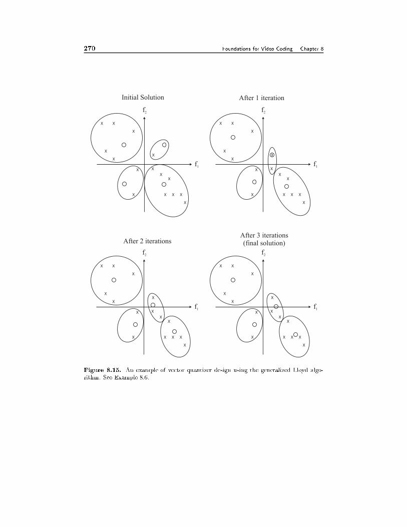
270 Foundations for Video Coding Chapter 8
f1 f1
f1 f1
f2 f2
f2 f2
x x
x x
x x
x x
x x
x x
x x
x x
x x
x x
x x
x x
x x
x x
x x
x x
x x
x x
x x
x x
x x
x x
x x
x x
x x
x x
x x
x x
x x
x x
Initial Solution After 1 iteration
After 2 iterationsAfter 3 iterations(final solution)
Figure 8.15. An example of vector quantizer design using the generalized Lloyd algo-
rithm. See Example 8.6.
Section 8.7. Summary 271
because the probability for codeword gl is P (Bl). Given the desired bit rate R and
vector dimension N , the optimization problem is to minimize Dq subject to
�Xl2L
P (Bl) log2 P (Bl) � RN: (8.6.19)
Using the Lagrange multiplier method, the above constrained optimization problem
can be converted to an unconstrained one:
minimize J(�) = Dq + �
�Xl2L
P (Bl) log2 P (Bl)�NR
!(8.6.20)
where � has to be chosen such that the constraint in Eq. (8.6.19) is satis�ed. For
each �xed �, the solution for gl and Bl can be obtained by using the generalized
Lloyd algorithm, with the distortion criterion changed from Dq to Eq. (8.6.20).
Then one can calculate the bit rate required by this solution using Eq. (8.6.18).
Essentially, di�erent � values yield solutions that are optimal for di�erent bit rates.
Under the entropy constraint, the optimal quantizers for a non-uniform source
tend to approach uniform when L is large. This way, the maximum distortion in
each partition region is similar. However, because the codewords that correspond
to regions with higher pdf will be more likely than others, they will be coded with
shorter codewords.
Note that the above discussion is equally applicable to scalar quantization. Re-
call that the distortion-rate function of any non-entropy-constrained MMSE quan-
tizer can be written in the form of Eq. (8.5.18) in the high rate case. The net e�ect
of applying entropy coding is to reduce the factor �2: For the Gaussian source, using
an entropy-constrained MMSE quantizer and scalar lossless coding can reduce �2
from 2.71 to 1.42, which corresponds to a saving of 0.467 bit/sample for the same
distortion. Compared to the RD bound for an i.i.d. Gaussian source, this represents
a gap of only 0.255 bit/sample from the bound [5, Sec. 4.6.2].
8.7 Summary
General Framework of Coding System (Sec. 8.1)
� A coding system usually consists of three components (Fig. 8.1): analysis
based on the source model, which converts the signal samples into model
parameters, quantization of the parameters (for lossy coding systems), and
binary encoding of quantized parameters.
� The main di�erence between di�erent coding systems lies in the source model
used. Video coding methods can be classi�ed into two groups, those using
source models that directly characterize the pixel values (waveform-based),
and those using models that describe the underlying object structures (content-
dependent).
272 Foundations for Video Coding Chapter 8
Bounds for Lossless and Lossy Coding (Sec. 8.3)
� The minimal rate required for lossless coding for a discrete source is deter-
mined by the source entropy rate (Th. 8.2).
� The minimal rate required for coding at a given distortion (the RD bound)
is determined by the minimal mutual information between the original source
and the quantized one (Th. 8.4).
� The above bounds are achievable only if in�nite number of samples are coded
together.
� Among all the sources with the same variance, the Gaussian source requires
the highest bit rate.
Binary Encoding (Sec. 8.4)
� Binary coding can be applied to a single sample at a time, a group of samples,
with or without conditioning based on previous samples.
� Hu�man and arithmetic coding are the two most popular methods for binary
encoding. Hu�man coders are simpler to design and operate, but cannot reach
the lossless coding bound with reasonable complexity. It is also hard to adapt
a Hu�man coder to variations in signal statistics. Arithmetic coders can more
easily approach the entropy bound and are more e�ective for non-stationary
signals, but they are also more complex to implement.
Scalar Quantization (Sec. 8.5)
� The necessary conditions for MSE optimality are the centroid condition, Eq. (8.5.13)
or Eq. (8.5.15), and the nearest neighbor condition, Eq. (8.5.12) or (8.5.14). A
locally optimal quantizer can be designed using the Lloyd algorithm (Fig. 8.9).
� With an MSE optimized quantizer, the operational RD function of a source
has the general form of Eq. (8.5.18) when the rate is suÆciently high. The
factor �2 depends on the pdf of the source.
� The MSE optimal quantizer above assume the quantized indices are coded
using �xed length coding. With variable length coding and when the rate
is suÆciently high, uniform quantization is nearly optimal. For image and
video coding, uniform quantization followed by entropy coding is preferred
over non-uniform quantization.
Vector Quantization (Sec. 8.6)
� VQ can exploit the correlation between samples and its eÆciency increases as
the vector dimension increases. It has the potential of reaching the RD bound
when the vector dimension reaches in�nity.
Section 8.8. Problems 273
� The computational complexity and storage requirement of a general uncon-
strained VQ encoder grows exponentially with the vector dimension. Practical
image and video coders use vector dimensions of 4� 4 or lower.
� The necessary conditions for MSE optimality are generalized version of the
centroid condition, Eq. (8.6.17) or Eq. (8.6.15), and the nearest neighbor
condition, Eq. (8.6.14). A locally optimal vector quantizer can be designed
using the generalized Lloyd algorithm (Fig. 8.14).
8.8 Problems
8.1 Consider a discrete source with an alphabet A = fa1; a2; : : : ; aLg: Compute
the entropy of the source for the following two cases:
(a) the source is uniformly distributed, with p(al) = 1=L;8l 2 L:(b) For a particular k 2 L, p(ak) = 1 and p(al) = 0; l 6= k:
8.2 Prove the relations given in Eqs. (8.2.6) to (8.2.12).
8.3 Prove the relations given in Eqs. (8.2.17) to (8.2.19).
8.4 Prove that the di�erential entropy of a Gaussian RV with mean � and variance
�2 is as given in Eq. (8.2.23).
8.5 Show that N -th order vector coding is worth than (N�1)-th order conditional
coding, if
1
NHN (F)�Hc;N01(F) >
N � 1
N:
8.6 A Markov source with three symbols A = fa1; a2; a3g has the following prob-ability distributions:
p(a1) = 1=2; p(a2) = 1=3; p(a3) = 1=6;
Pfai=ajg =�
12if i = j;
14otherwise:
(a) Calculate the 1st order entropy, 2nd order entropy, 1st order conditional
entropy, and the entropy rate of this source;
(b) Design the 1st order, 2nd order, and 1st order conditional Hu�man codes
for this source. Calculate the resulting bit rate for each case. Compare it to
the corresponding lower and upper bounds de�ned by the entropy.
(c) What is the minimal bit rate achievable with this source? How could you
achieve the minimal rate?
274 Foundations for Video Coding Chapter 8
8.7 Encode and decode the following sequence using arithmetic coding. Using the
occurrence frequency of each symbol in the sequence as the estimate of the
probability of the symbol.
Source sequence: a c b a a b a c a c b a
What is bit rate of the coded sequence? Compare the result to scalar Hu�man
coding.
8.8 Show that for a MMSE quantizer, the original RV F , the quantized RV G and
the quantization error Q = F � G satisfy the following statistical relations:
(a) The quantized value is an unbiased estimate of the original value: EfGg =EfFg(b) The quantized value is orthogonal to the quantization error: EfGQg = 0
(c) The quantization process reduces the signal variance: �2G = �2F � �2Q:
8.9 Show that the MMSE quantizer for a uniform source is given by Eq. (8.5.7).
8.10 Prove that for a source with arbitrary mean � and variance �2, the optimal
reconstruction and boundary values can be obtained from those derived for a
source with zero mean and unit variance according to Eq. (8.5.17).
8.11 Consider a RV F with pdf p(f) = �
2e��jf j. A three level quantizer is de�ned
as
Q(f) =
8<:
b f > a
0 �a � f � a
�b f < �a(a) Find b for a given a such that the centroid condition is satis�ed when the
distortion measure is the MSE.
(b) Find a for a given b such that the nearest neighbor condition is met.
(c) Find an optimal set of a; b in terms of � such that both conditions are
satis�ed. Derive the �nal MSE.
8.12 The optimality conditions given in Eqs. (8.5.12) and (8.5.13) are derived by
minimize the MSE. Here we consider other distortion measures.
(a) Derive a similar set of equations if the distortion criterion is the mean
absolute error (MAE), i.e., Dq = EfjF �Q(F)jg: Show that the generalized
centroid gl for the decision region Bl = [bl�1; bl) isZgl
bl�1
p(f jf 2 Bl)df =
Zbl
gl
p(f jf 2 Bl)df:
That is, gl equally splits Bl. Such a gl is also called the median of the region
Bl. What is the form of the nearest neighbor condition under this distortion
measure?
Section 8.8. Problems 275
(b) For a source with Laplacian distribution, p(f) = 12e�jf j; determine the
generalized centroid for the region Bl under the MAE criterion. Compare this
centroid to that determined based on the MSE criterionDq = EfjF�Q(F)j2g:8.13 Consider a quantizer for a discrete vector source S = ffk; k = 1; 2; : : : ;Kg,
where fk is an N -D vector. Suppose the distortion measure between two
vectors is the Hamming distance de�ned as
d(f ;g) =
�0 if f = g;
1 otherwise:
Assume these vectors are to be quantized into L < K codewords.
(a) For a given partition region of the source, Bl = ffk; k = 1; 2; : : : ;Klg;determine a new codeword for this region based on the centroid rule.
(b) For a given set of codewords C = fg1;g2; : : : ;gLg; determine a new parti-
tion of the source based on the nearest neighbor rule. Is the partition unique?
(c) Starting from an arbitrary initial partition of the source, how many itera-
tions are needed to arrive at a locally optimal codebook ?
Hint: Consider two separate cases: 1) when all the training vectors are di�er-
ent from each other; 2) when some of the training vectors are the same.
8.14 A 2-D vector quantizer has two codewords: g1 = [1=2; 1=2];g2 = [�1=2;�1=2]:Suppose the input vectors f = [f1; f2] are uniformly distributed in the square
de�ned by �1 < f1 < 1 and �1 < f2 < 1. Illustrate the partition regions
associated with the two codewords and determine the MSE of this quantizer
(you could just write down the integral formula).
8.15 A 2-D lattice quantizer over a �nite region is composed of the codewords
(g1; g2) de�ned by g1 = m and g2 = m+2n, where m;n are integers such that
(g1; g2) fall in the speci�ed region.
(a) Sketch the codewords and partition regions near the origin.
(b) Design an algorithm that will identify the nearest codeword for any given
input point in the plane.
(c) Find the nearest codeword for the point (123:4; 456:7).
(d) Determine the MSE of this quantizer if the input is uniformly distributed
in the space spanned by all the partition regions.
8.16 Write a C or Matlab code to implement the generalized Lloyd algorithm based
on training data generated from a 2-D i.i.d. Gaussian source. Assume the two
components in each sample are independent and both have zero mean and
unit variance. You can choose the number of samples used and the codebook
size. Indicate the training samples and the codewords after each iteration
using crosses and circles in a 2-D plot.
276 Foundations for Video Coding Chapter 8
8.17 Repeat the above problem, but assume the two vector components are cor-
related with a correlation coeÆcient �. Compare the results obtained with
di�erent values of �:
8.9 Bibliography
[1] T. Berger. Rate Distortion Theory. Prentice Hall, Englewood Cli�s, NJ, 1971.
[2] J.H. Conway and N.J. A. Sloane. Fast quantizing and decoding algorithms for
lattice quantizers and codes. IEEE Trans. Inform. Theory, IT-28:227{232, Mar.
1982.
[3] T. M. Cover and J. A. Thomas. Elements of Information Theory. John Wiley
& Sons, New York, 1991.
[4] A. Gersho and R. M. Gray. Vector Quantization and Signal Compression.
Kluwer Academic Press, 1992.
[5] N. S. Jayant and P. Noll. Digital Coding of Waveforms. Prentice-Hall, Inc.,
1984.
[6] Y. Linde, A. Buzo, and R. M. Gray. An algorithm for vector quantizer design.
IEEE Trans. Commun., 28:84{95, Jan. 1980.
[7] P. S. Lloyd. Least squares quantization in PCM. IEEE Trans. Inform. Theory,
IT-28, Mar. 1982. Originally published as Bell Labotories Technical Note, 1957.
[8] J. MacQueen. Some methods for classi�cation and analysis of multivariat obser-
vations. In Fifth Berkeley Symposium on Math. Stat. and Prob., volume 1, pages
281{296, 1967.
[9] K. Sayood. Introduction to Data Compression. Morgan Kaufmann Publishers,
Inc., San Francisco, CA, 1996.
[10] T. A. Welch. A technique for high performance data compression. Computer,
pages 8{18, 1984.
[11] I. H. Witten, R. M. Neal, and J. G. Cleary. Arithmetic coding for data com-
pression. Commun. ACM, 30:520{540, 1987.
[12] J. Ziv and A. Lempel. A universal algorithm for sequential data compression.
IEEE Trans. Inform. Theory, IT-23:149{162, May 1979.
Chapter 9
WAVEFORM-BASED VIDEO
CODING
In Chap. 8, we introduced the fundamental techniques for video coding that are
common in both waveform-based and content-dependent coders. In this chapter, we
focus on techniques for waveform-based video coding. First we describe block-based
transform coding techniques (Sec. 9.1), by which each block of pixels are converted
into a set of uncorrelated coeÆcients, which are then quantized and coded. We will
introduce the important Karhunen-Loeve transform (KLT) and its approximation,
the discrete cosine transform (DCT), which is used in most modern image coding
standards. A coding method using another important transform, wavelet transform,
is introduced in Sec. 11.3, when we describe scalable coding. In Sec. 9.2, we intro-
duce coding techniques using spatial and temporal prediction. These techniques
reduce the data rate of a video sequence by exploiting spatial correlation between
neighboring pixels as well as temporal correlation between consecutive frames of
an video sequence. The spatial correlation is due to the fact that color values of
adjacent pixels in the same video frame usually change smoothly. The temporal
correlation refers to the fact that consecutive frames of a sequence usually show
the same physical scene, occupied by the same objects that may have moved. We
conclude this chapter by presenting a coding scheme that combines transform and
predictive coding (Sec. 9.3), which is a popular and e�ective technique and has been
adopted by all international video coding standards.
9.1 Block-Based Transform Coding
Transform coding has proven to be specially e�ective for compression of still images
and video frames. Ideally, a transform should be applied to an entire image or video
frame, to fully exploit the spatial correlation among pixels. But to reduce compu-
tational complexity, block-based transform coding is more often used in practice,
which divides an image into non-overlapping blocks, and applies the transform over
each block. In this chapter, we only describe block-based transform coding, with
focus on the type of algorithm used in standard image and video coders. For a more
277
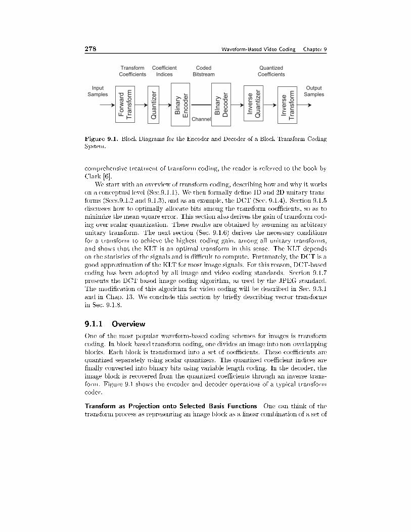
278 Waveform-Based Video Coding Chapter 9
For
war
dT
rans
form
Qua
ntiz
er
Bin
ary
Enc
oder
Inve
rse
Tra
nsfo
rm
Inve
rse
Qua
ntiz
er
BIn
ary
Dec
oder
InputSamples
CoefficientIndices
TransformCoefficients
OutputSamples
CodedBitstream
QuantizedCoefficients
Channel
Figure 9.1. Block Diagrams for the Encoder and Decoder of a Block Transform Coding
System.
comprehensive treatment of transform coding, the reader is referred to the book by
Clark [6].
We start with an overview of transform coding, describing how and why it works
on a conceptual level (Sec.9.1.1). We then formally de�ne 1D and 2D unitary trans-
forms (Secs.9.1.2 and 9.1.3), and as an example, the DCT (Sec. 9.1.4). Section 9.1.5
discusses how to optimally allocate bits among the transform coeÆcients, so as to
minimize the mean square error. This section also derives the gain of transform cod-
ing over scalar quantization. These results are obtained by assuming an arbitrary
unitary transform. The next section (Sec. 9.1.6) derives the necessary conditions
for a transform to achieve the highest coding gain, among all unitary transforms,
and shows that the KLT is an optimal transform in this sense. The KLT depends
on the statistics of the signals and is diÆcult to compute. Fortunately, the DCT is a
good approximation of the KLT for most image signals. For this reason, DCT-based
coding has been adopted by all image and video coding standards. Section 9.1.7
presents the DCT-based image coding algorithm, as used by the JPEG standard.
The modi�cation of this algorithm for video coding will be described in Sec. 9.3.1
and in Chap. 13. We conclude this section by brie y describing vector transforms
in Sec. 9.1.8.
9.1.1 Overview
One of the most popular waveform-based coding schemes for images is transform
coding. In block-based transform coding, one divides an image into non-overlapping
blocks. Each block is transformed into a set of coeÆcients. These coeÆcients are
quantized separately using scalar quantizers. The quantized coeÆcient indices are
�nally converted into binary bits using variable length coding. In the decoder, the
image block is recovered from the quantized coeÆcients through an inverse trans-
form. Figure 9.1 shows the encoder and decoder operations of a typical transform
coder.
Transform as Projection onto Selected Basis Functions One can think of the
transform process as representing an image block as a linear combination of a set of
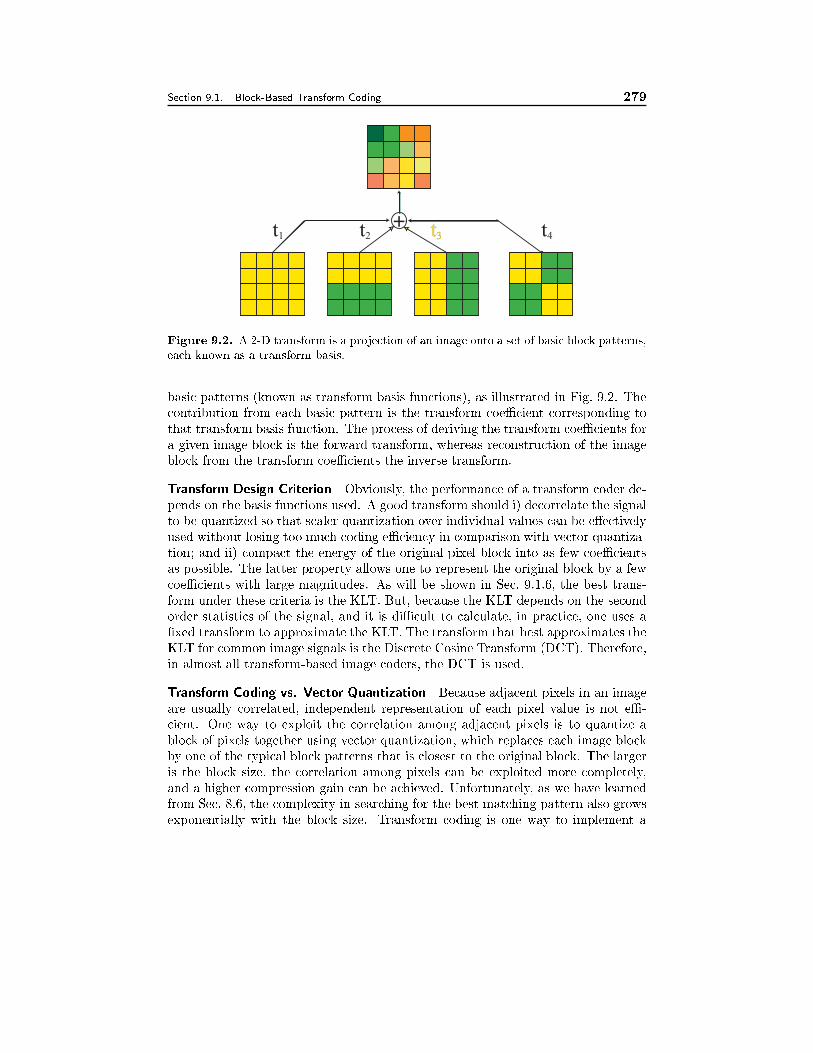
Section 9.1. Block-Based Transform Coding 279
+t1 t2 t3 t4
Figure 9.2. A 2-D transform is a projection of an image onto a set of basic block patterns,
each known as a transform basis.
basic patterns (known as transform basis functions), as illustrated in Fig. 9.2. The
contribution from each basic pattern is the transform coeÆcient corresponding to
that transform basis function. The process of deriving the transform coeÆcients for
a given image block is the forward transform, whereas reconstruction of the image
block from the transform coeÆcients the inverse transform.
Transform Design Criterion Obviously, the performance of a transform coder de-
pends on the basis functions used. A good transform should i) decorrelate the signal
to be quantized so that scaler quantization over individual values can be e�ectively
used without losing too much coding eÆciency in comparison with vector quantiza-
tion; and ii) compact the energy of the original pixel block into as few coeÆcients
as possible. The latter property allows one to represent the original block by a few
coeÆcients with large magnitudes. As will be shown in Sec. 9.1.6, the best trans-
form under these criteria is the KLT. But, because the KLT depends on the second
order statistics of the signal, and it is diÆcult to calculate, in practice, one uses a
�xed transform to approximate the KLT. The transform that best approximates the
KLT for common image signals is the Discrete Cosine Transform (DCT). Therefore,
in almost all transform-based image coders, the DCT is used.
Transform Coding vs. Vector Quantization Because adjacent pixels in an image
are usually correlated, independent representation of each pixel value is not eÆ-
cient. One way to exploit the correlation among adjacent pixels is to quantize a
block of pixels together using vector quantization, which replaces each image block
by one of the typical block patterns that is closest to the original block. The larger
is the block size, the correlation among pixels can be exploited more completely,
and a higher compression gain can be achieved. Unfortunately, as we have learned
from Sec. 8.6, the complexity in searching for the best matching pattern also grows
exponentially with the block size. Transform coding is one way to implement a
280 Waveform-Based Video Coding Chapter 9
constrained vector quantizer without using an exhaustive search. Speci�cally, the
codewords in this quantizer are those representable by linear combinations of basis
vectors with quantized coeÆcients. Because each coeÆcient depends on the entire
image block, scalar quantization of the transform coeÆcients essentially accom-
plishes vector quantization of the entire block, but at a reduced complexity.
9.1.2 1-D Unitary Transform
General 1-D Linear Transform
As described already, the transform process can be thought of as decomposing
an image block into a set of basic block patterns. This is in fact a 2-D linear
transform. Before formally de�ning the 2-D transform, we �rst de�ne 1-D transform.
In this case, a 1-D signal is divided into vectors of length N , and each vector
is represented as a linear combination of a set of basis vectors. Each transform
coeÆcient represents the contribution from one basis vector. Mathematically, these
coeÆcients are obtained by a matrix operation. Let s = [s1; s2; : : : ; sN ]T represent
the vector consists of original samples, t = [t1; t2; : : : ; tN ]T the vector containing
all the transformed coeÆcients. Further, let uk = [uk;1; uk;2; : : : ; uk;N ]T denote
the vector corresponding to the k-th transform basis and [U] = [u1;u2; : : : ;uN ]
the matrix containing all basis vectors. Then the inverse transform represents the
sample vector s as
Inverse Transform: s =Xk2N
tkuk = [U]t (9.1.1)
where N = f1; 2; : : : ; Ng: In order to be able to represent any N -D vector with
N basis vectors, the basis vectors must be linearly independent. In this case, the
matrix [U] must be invertible and the transform coeÆcients can be determined by
Forward Transform: t = [U]�1s = [V]s (9.1.2)
For generality, we assume that the basis vectors uk may contain complex com-
ponents, so that uk belongs to the N -D complex space CN . In this case, even if s
is a real vector, t is in general a complex vector. In the remaining discussion we
assume both s and t belong to CN :
1-D Unitary Transform
The above discussion does not impose any constraint on the transform basis vectors.
A special class of linear transform is the unitary transform, in which the basis vectors
are orthonormal to each other.
Before formally de�ning the unitary transform, we �rst review the de�nition of
inner product and norm in a complex space CN . The inner product of two vectors
s1; s2, both in CN , are de�ned as
< s1; s2 >= sH1 s2 =Xn2N
s�1;ns2;n; (9.1.3)
Section 9.1. Block-Based Transform Coding 281
where the superscript H denotes vector transpose followed by element conjugation.
Two vectors are said to be orthogonal to each other if < s1; s2 >= 0: The norm kskof s 2 CN is de�ned as
ksk2 =< s; s >=Xn2N
jsnj2: (9.1.4)
The norm ksk represents the length or magnitude of s, and the norm square ksk2the energy of s: A vector with a unit norm is said to be a normalized vector. If two
vectors are orthogonal to each other, and each is normalized, they are said to be
orthonormal.
If the basis vectors in the linear transform de�ned in Eq. (9.1.2) are orthonormal
with each other, i.e.,
< uk;ul >=Xn2N
u�k;nul;n = Æk;l =
�1 if k = l;
0 if k 6= l;(9.1.5)
then the matrix [U] satis�es
[U]H[U] = [U][U]
H= [I]N (9.1.6)
where [I]N represents an N � N identity matrix. A matrix satisfying the above
condition is called unitary. A linear transform where the transform matrix [U] is
unitary is called a unitary transform. In this case, [U]�1
= [U]Hand the transform
coeÆcients can be found by t = [U]Hs or tk =< uk; s >= uHk s: That is, the k-th
transform coeÆcient tk can be found simply by the inner product of s with uk.
To summarize, a unitary transform pair is speci�ed by
Forward transform: tk =< uk; s > or t = [U]Hs = [V]s
Inverse transform: s =Pk2N tkuk = [U]t = [V]Ht:
(9.1.7)
Usually, we refer to a transform by its forward transform matrix [V] = [U]H. The
basis vectors of the transform are the conjugate of the row vectors in [V].
Example 9.1 (1-D DFT) Recall that the N-point DFT is speci�ed by
Forward transform: tk =1pN
PN�1n=0
sne�j2�kn=N
; k = 0; 1; : : : ; N � 1;
Inverse transform: sn = 1pN
PN�1k=0
tkej2�kn=N
; n = 0; 1; : : : ; N � 1:(9.1.8)
Using the notation described here, we see that it is a unitary transform with basis vectors
de�ned by:
uk;n =1pNej2� kn
N ; n = 0; 1; : : : ; N � 1; k = 0; 1; : : : ; N � 1; (9.1.9)
or
uk =1pN
h1 e
j2� kN � � � e
j2�k(N�1)
N
iT; k = 0; 1; : : : ; N � 1: (9.1.10)
Note that in this example, we follow the convention of using an index range of 0 to N � 1
for k and n, instead of 1 to N .
282 Waveform-Based Video Coding Chapter 9
Properties of Unitary Transforms
Until now, we have assumed that s is a given sample vector, and t is its transform.
In reality, s is a realization of a random vector S = [S1;S2; : : : ;SN ]T ; which cor-
responds to any N samples extracted from a source. Similarly, t is a realization
of a random vector T = [T1; T2; : : : ; TN ]T = [V]S : In transform coding, we are
interested in not only the relations between s and t, but also relations between the
statistics of S and T : With an unitary transform, the following relations exist.
1. The mean vectors �s = EfSg and �t = EfT g are related by
�t = [V]�s; �s = [V]H�t: (9.1.11)
The covariance matrices [C]s = Ef(S � �s)(S � �s)Hg and [C]t = Ef(T �
�t)(T � �t)Hg are related by:
[C]t = [V][C]s[V]H ; [C]s = [V]H [C]t[V]: (9.1.12)
2. The total energy of the transformed vector equals that of the sample vector.
This is true both for a given realization and the ensemble average, i.e.,Xn2N
s2n =Xk2N
t2k; (9.1.13)
Xn2N
�2s;n =Xk2N
�2t;k: (9.1.14)
where �2s;n = Ef(Sn � �s;n)2g and �2t;k = Ef(Tk � �t;k)2g are the variances ofSn and Tk, respectively.This property is equivalent to the Parseval's theorem for the Fourier trans-
form.
3. Suppose we use only the �rst K � N coeÆcients to approximate s, with the
approximated vector being sK =PKk=1 tkuk; the approximation error signal
is e = s� sK =PNk=K+1 tkuk: The approximation error energy for a given s
is
kek2 =Xn2N
e2n =
NXk=K+1
t2k: (9.1.15)
The variance of E = S � S over the ensemble of S is
EfkEk2g =Xn2N
�2e;n =
NXk=K+1
�2t;k: (9.1.16)
Because the sum of all coeÆcient squares or variances is a constant (Eq. (9.1.13)
or (9.1.14)), the approximation error for a particular signal vector is mini-
mized if one choosesK coeÆcients that have the largest values to approximate
the original signal. Similarly, the mean approximation error is minimized by
choosing K coeÆcients with the largest variances.
Section 9.1. Block-Based Transform Coding 283
The proof of the above relations is quite straight-forward, and is left as an
exercise (Prob. 9.1).
9.1.3 2-D Unitary Transform
The above discussion has assumed that the input samples are from a 1-D signal.
For a 2-D image block, the above descriptions still apply if we think of s as a vector
consisting of the samples from an image block arranged in a 1-D order, and each ukas a vector representation of a basis image, using the same 1-D ordering. However,
one can also extend the de�nition of the 1-D transform to 2-D. In this case, an
M �N image block [S] = [Sm;n] is represented as a linear combination of M �N
basis images [U]k;l = [Uk;l;m;n] as (cf. Fig. 9.2)
[S] =Xk2M
Xl2N
Tk;l[U]k;l; (9.1.17)
where M = f1; 2; : : : ;Mg;N = f1; 2; : : : ; Ng:Let CM�N represent theM�N dimensional complex space. Let [S]1 = [S1;m;n];
[S]2 = [S2;m;n] be two matrices in this space. Then the inner product of the two are
de�ned by:
< [S]1; [S]2 >=Xm2M
Xn2N
S�1;m;nS2;m;n: (9.1.18)
The norm of a matrix [S] = [Sm;n] is de�ned as:
k[S]k2 =< [S]; [S] >=Xm2M
Xn2N
jSm;nj2: (9.1.19)
With above de�nitions, a set of basis images [U]k;l; k 2 M; l 2 N ; are said to be
orthonormal with each other, if
< [U]k;l; [U]i;j >= Æk;iÆl;j =
�1; if k = i; l = j;
0 otherwise:(9.1.20)
With an orthonormal set of basis images, one can easily �nd the transform
coeÆcient by Tk;l =< [U]k;l; [S] > : The forward and inverse transform relations
for an M �N 2-D unitary transforms are
Forward transform: Tk;l =< [U]k;l; [S] >;
Inverse Transform: [S] =Pk2M
Pl2N Tk;l[U]k;l:
(9.1.21)
Example 9.2 (2-D DFT) The 2-D DFT of length M �N is de�ned as:
Forward transform: Tk;l =1pMN
PM�1m=0
PN�1n=0
Sm;ne�j2�( km
M+ lnN);
k = 0; 1; : : : ;M � 1; l = 0; 1; : : : ; N � 1;
Inverse transform: Sm;n = 1pMN
PM�1k=0
PN�1l=0
Tk;lej2�( km
M+ lnN);
m = 0; 1; : : : ;M � 1; n = 0; 1; : : : ; N � 1:
(9.1.22)
284 Waveform-Based Video Coding Chapter 9
One can see that the above transform is a 2-D unitary transform with basis images
de�ned by:
[U]k;l;m;n =1pMN
ej2�(kmM
+ lnN);m; k = 0; 1; : : : ;M � 1; n; l = 0; 1; : : : ; N � 1:
(9.1.23)
Separable Transforms
One particularly important class of 2-D transforms are those in which each basis
image is the outer-product of two basis vectors each from a 1-D transform. Virtually
all the 2-D transforms in use belong to this type. Speci�cally, let hk; k 2 M and
gl; l 2 N represent basis vectors in CM and CN respectively, then one can form
basis images in CM�N by:
[U]k;l = hkgTl or [U]k;l;m;n = hk;mgl;n; k 2M; l 2 N : (9.1.24)
It can be shown that [U]k;l will form an orthonormal basis set in CM�N as long as
hk and gl form orthonormal basis sets in CM and CN , respectively.
Example 9.3 (2-D DFT as separable transforms) Recall that the basis im-
ages for M �N point 2-D DFT are:
Uk;l;m;n =1pMN
ej2�(kmM
+ lnN);
whereas the basis vectors for M-point DFT and N-point DFT are respectively
hk;m =1pMej2�
kmM ; gl;n =
1pNej2�
lnN :
Obviously, Uk;l;m;n = hk;mgl;n. Therefore, the M�N-point 2-D DFT is a separable
transform constructed from an M-point 1-D DFT and an N-point 1-D DFT.
When the transform is separable, one can �rst accomplish 1-D transform for each
row using basis matrix [G] = [g1;g2; : : : ;gN ], and then perform 1-D transform for
each column of the intermediate image using basis matrix [H] = [h1;h2; : : : ;hM ].
This operation can be represented as
Forward Transform: [T] = [H]H[S][G];
Inverse Transform: [S] = [H][S][G]H:
(9.1.25)
When a 2-D transform is separable, its equivalent 1-D transform representation
will have a transform matrix that is the Kronecker product of the matrix [G] and
[H]: For more detailed discussion on this topic and additional properties of separable
transforms, see [18, Sec. 5.2].
Section 9.1. Block-Based Transform Coding 285
Computational savings of separable transforms An M �N transform in general
takesM �N calculations for determining each coeÆcient. To determine all M �NcoeÆcients, the total number of calculations is M2N2, which becomes N4 when
M = N: On the other hand, when the transform is separable, one �rst calculates
N -point 1-D transform along each of M rows, each requiring N2 calculations. One
then calculates M -pt 1-D transform along each of N columns, each requiring M2
calculations. The total number of calculations is MN2 + NM2, which is 2N3 if
M = N: When N is large, the reduction from N4 to 2N3 is signi�cant.
If there exists a fast algorithm for calculating the 1-D transform, then further
savings are obtainable. For example, if an N -point 1-D transform takes N log2N
operations, then an N � N 2-D separable transform can be done in 2N2 logN
operations.
9.1.4 Signal Independent Transforms and the DCT
Besides the DFT, there are many other transforms that have been developed for
signal analysis, including Discrete Cosine Transform (DCT), Discrete Sine Trans-
form (DST), Hadamard Transform, Walsh Transform, Haar Transform, Slant Trans-
forms. See [12] or [18] for de�nitions of the basis vectors of these transforms. All
these transforms are originally de�ned in the 1-D form, and can be used to construct
2-D separable transforms. The DFT is most widely used for performing frequency
domain analysis for discrete signals. On the other hand, the DCT has been found
to be more useful for source coding, especially image coding. For this reason, we
introduce the DCT in this section and show examples of representing images using
DCT.
The basis vectors of the 1-D N -point DCT are de�ned by:
uk;n = �(k) cos(2n+ 1)k�
2N;n = 0; 1; : : : ; N � 1 (9.1.26)
with
�(k) =
8<:q
1N
k = 0q2N
k = 1; 2; : : : ; N � 1:(9.1.27)
(9.1.28)
The forward and inverse transforms are described by:
tk =
N�1Xn=0
u�k;nsn = �(k)
N�1Xn=0
sn cos(2n+ 1)k�
2N; (9.1.29)
sn =
N�1Xk=0
uk;ntk =
N�1Xk=0
�(k)tk cos(2n+ 1)k�
2N(9.1.30)
As with the DFT, we follow the convention of using an index range of 0 to N � 1
for k and n.
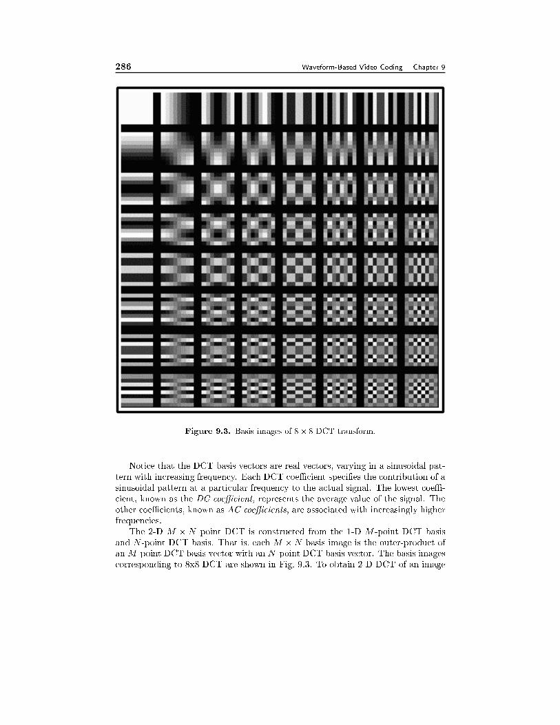
286 Waveform-Based Video Coding Chapter 9
Figure 9.3. Basis images of 8 � 8 DCT transform.
Notice that the DCT basis vectors are real vectors, varying in a sinusoidal pat-
tern with increasing frequency. Each DCT coeÆcient speci�es the contribution of a
sinusoidal pattern at a particular frequency to the actual signal. The lowest coeÆ-
cient, known as the DC coeÆcient, represents the average value of the signal. The
other coeÆcients, known as AC coeÆcients, are associated with increasingly higher
frequencies.
The 2-D M � N point DCT is constructed from the 1-D M -point DCT basis
and N -point DCT basis. That is, each M �N basis image is the outer-product of
anM -point DCT basis vector with an N -point DCT basis vector. The basis images
corresponding to 8x8 DCT are shown in Fig. 9.3. To obtain 2-D DCT of an image
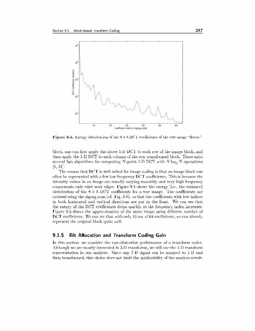
Section 9.1. Block-Based Transform Coding 287
10 20 30 40 50 60
102
103
104
105
106
coefficient index in zigzag order
DC
T c
oeffi
cien
t var
ianc
e
Figure 9.4. Energy distribution of the 8� 8 DCT coeÆcients of the test image \ ower".
block, one can �rst apply the above 1-D DCT to each row of the image block, and
then apply the 1-D DCT to each column of the row transformed block. There exist
several fast algorithms for computing N -point 1-D DCT with N log2N operations
[4, 21].
The reason that DCT is well suited for image coding is that an image block can
often be represented with a few low frequency DCT coeÆcients. This is because the
intensity values in an image are usually varying smoothly and very high frequency
components only exist near edges. Figure 9.4 shows the energy (i.e., the variance)
distribution of the 8 � 8 DCT coeÆcients for a test image. The coeÆcients are
ordered using the zigzag scan (cf. Fig. 9.8), so that the coeÆcients with low indices
in both horizontal and vertical directions are put in the front. We can see that
the energy of the DCT coeÆcients drops quickly as the frequency index increases.
Figure 9.5 shows the approximation of the same image using di�erent number of
DCT coeÆcients. We can see that with only 16 out of 64 coeÆcients, we can already
represent the original block quite well.
9.1.5 Bit Allocation and Transform Coding Gain
In this section, we consider the rate-distortion performance of a transform coder.
Although we are mostly interested in 2-D transforms, we will use the 1-D transform
representation in our analysis. Since any 2-D signal can be mapped to 1-D and
then transformed, this choice does not limit the applicability of the analysis result.
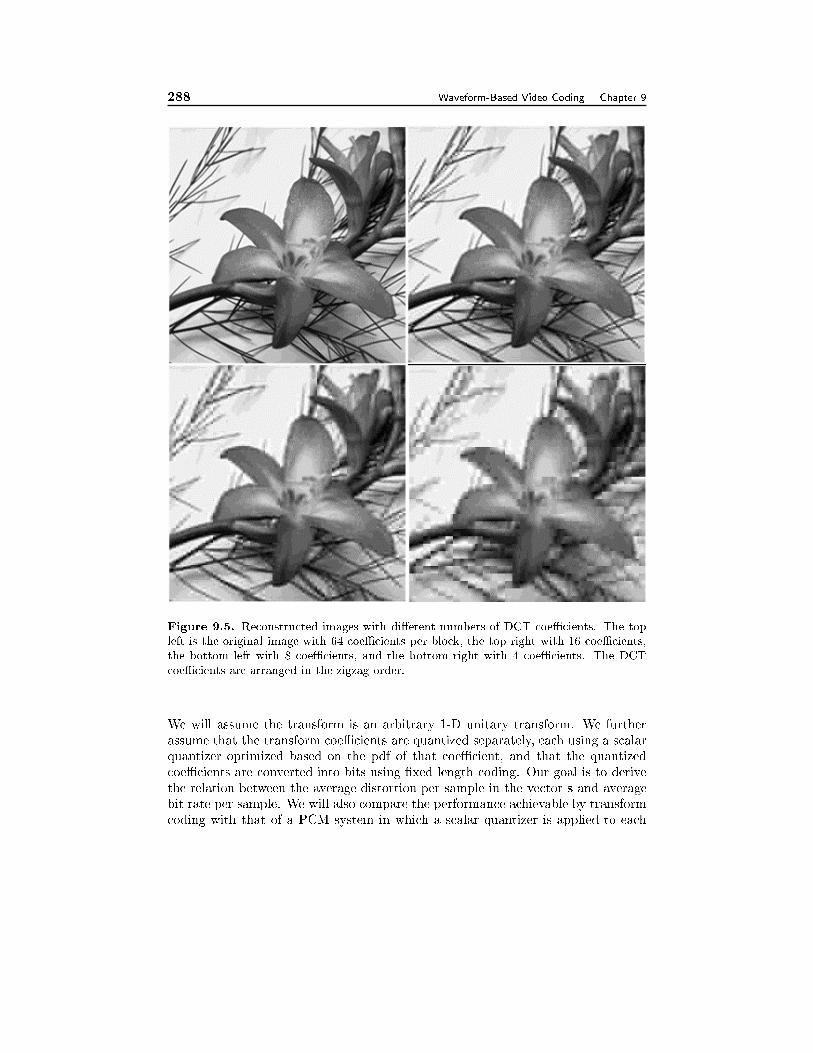
288 Waveform-Based Video Coding Chapter 9
Figure 9.5. Reconstructed images with di�erent numbers of DCT coeÆcients. The top
left is the original image with 64 coeÆcients per block, the top right with 16 coeÆcients,
the bottom left with 8 coeÆcients, and the bottom right with 4 coeÆcients. The DCT
coeÆcients are arranged in the zigzag order.
We will assume the transform is an arbitrary 1-D unitary transform. We further
assume that the transform coeÆcients are quantized separately, each using a scalar
quantizer optimized based on the pdf of that coeÆcient, and that the quantized
coeÆcients are converted into bits using �xed length coding. Our goal is to derive
the relation between the average distortion per sample in the vector s and average
bit rate per sample. We will also compare the performance achievable by transform
coding with that of a PCM system in which a scalar quantizer is applied to each
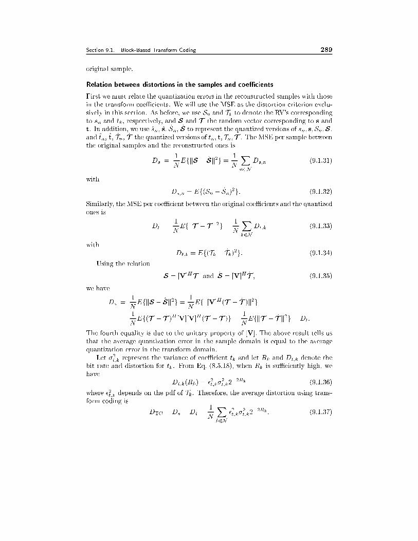
Section 9.1. Block-Based Transform Coding 289
original sample.
Relation between distortions in the samples and coeÆcients
First we must relate the quantization errors in the reconstructed samples with those
in the transform coeÆcients. We will use the MSE as the distortion criterion exclu-
sively in this section. As before, we use Sn and Tk to denote the RV's correspondingto sn and tk, respectively, and S and T the random vector corresponding to s and
t. In addition, we use sn, s, Sn, S to represent the quantized versions of sn; s;Sn;S,and tn, t, Tn, T the quantized versions of tn; t; Tn;T . The MSE per sample between
the original samples and the reconstructed ones is
Ds =1
NEfkS � Sk2g = 1
N
Xn2N
Ds;n (9.1.31)
with
Ds;n = Ef(Sn � Sn)2g: (9.1.32)
Similarly, the MSE per coeÆcient between the original coeÆcients and the quantized
ones is
Dt =1
NEfkT � T k2g = 1
N
Xk2N
Dt;k (9.1.33)
with
Dt;k = Ef(Tk � Tk)2g: (9.1.34)
Using the relation
S = [V]HT and S = [V]H T ; (9.1.35)
we have
Ds =1
NEfkS � Sk2g = 1
NEfk[V]H(T � T )k2g
=1
NEf(T � T )H [V][V]H (T � T )g = 1
NEfkT � T k2g = Dt:
The fourth equality is due to the unitary property of [V]: The above result tells us
that the average quantization error in the sample domain is equal to the average
quantization error in the transform domain.
Let �2t;k represent the variance of coeÆcient tk and let Rk and Dt;k denote the
bit rate and distortion for tk. From Eq. (8.5.18), when Rk is suÆciently high, we
have
Dt;k(Rk) = �2t;k�2t;k2
�2Rk (9.1.36)
where �2t;k depends on the pdf of Tk. Therefore, the average distortion using trans-
form coding is
DTC = Ds = Dt =1
N
Xk2N
�2t;k�2t;k2
�2Rk : (9.1.37)
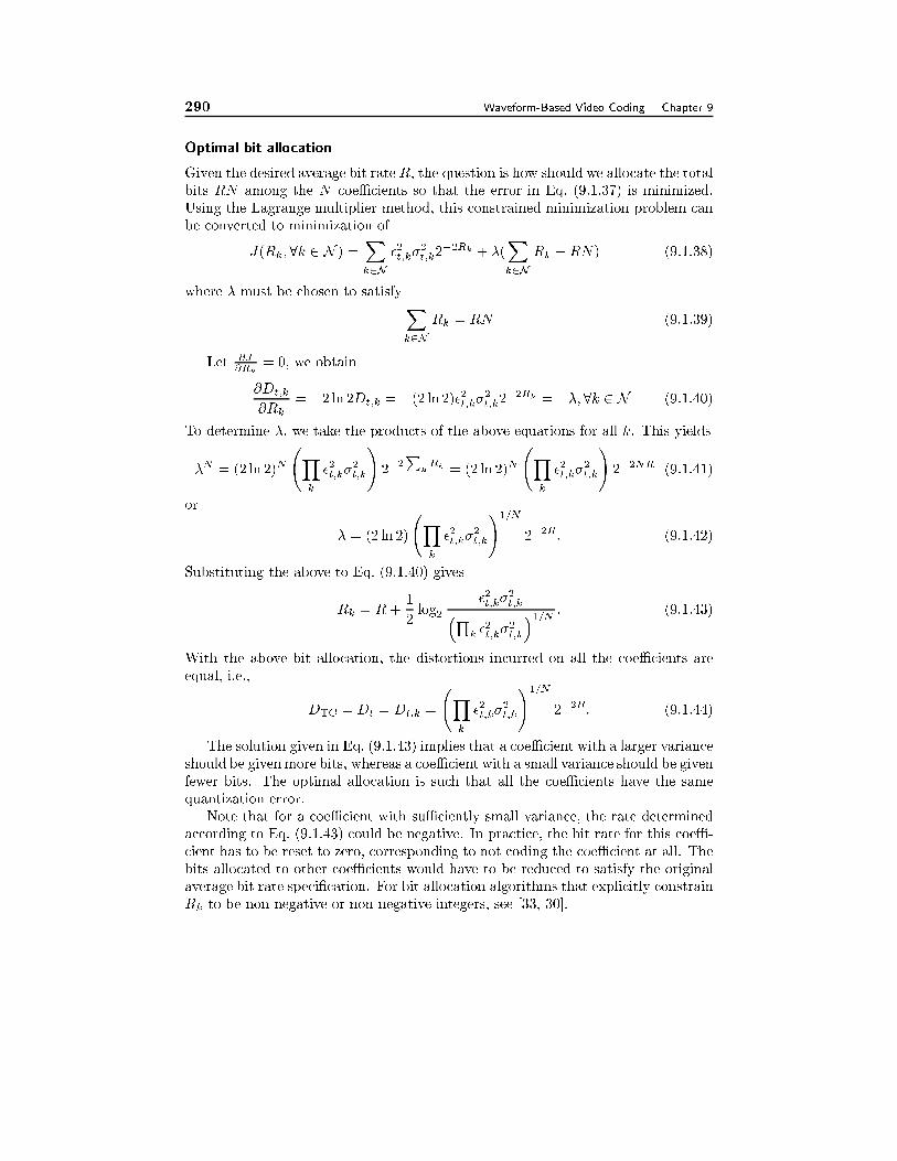
290 Waveform-Based Video Coding Chapter 9
Optimal bit allocation
Given the desired average bit rate R, the question is how should we allocate the total
bits RN among the N coeÆcients so that the error in Eq. (9.1.37) is minimized.
Using the Lagrange multiplier method, this constrained minimization problem can
be converted to minimization of
J(Rk;8k 2 N ) =Xk2N
�2t;k�2t;k2
�2Rk + �(Xk2N
Rk �RN) (9.1.38)
where � must be chosen to satisfyXk2N
Rk = RN (9.1.39)
Let @J@Rk
= 0, we obtain
@Dt;k
@Rk= �2 ln 2Dt;k = �(2 ln 2)�2t;k�2t;k2�2Rk = ��;8k 2 N (9.1.40)
To determine �, we take the products of the above equations for all k. This yields
�N = (2 ln 2)N
Yk
�2t;k�2t;k
!2�2P
kRk = (2 ln 2)N
Yk
�2t;k�2t;k
!2�2NR (9.1.41)
or
� = (2 ln 2)
Yk
�2t;k�2t;k
!1=N
2�2R: (9.1.42)
Substituting the above to Eq. (9.1.40) gives
Rk = R+1
2log2
�2t;k�2t;k�Q
k �2t;k�
2t;k
�1=N : (9.1.43)
With the above bit allocation, the distortions incurred on all the coeÆcients are
equal, i.e.,
DTC = Dt = Dt;k =
Yk
�2t;k�2t;k
!1=N
2�2R: (9.1.44)
The solution given in Eq. (9.1.43) implies that a coeÆcient with a larger variance
should be given more bits, whereas a coeÆcient with a small variance should be given
fewer bits. The optimal allocation is such that all the coeÆcients have the same
quantization error.
Note that for a coeÆcient with suÆciently small variance, the rate determined
according to Eq. (9.1.43) could be negative. In practice, the bit rate for this coeÆ-
cient has to be reset to zero, corresponding to not coding the coeÆcient at all. The
bits allocated to other coeÆcients would have to be reduced to satisfy the original
average bit rate speci�cation. For bit allocation algorithms that explicitly constrain
Rk to be non-negative or non-negative integers, see [33, 30].
Section 9.1. Block-Based Transform Coding 291
Transform Coding Gain over PCM
Assume that the original samples come from a stationary source so that each sample
has the same variance �2s . If we apply optimal scalar quantization to individual
samples separately, then the distortion is related to the rate by
DPCM = Ds;n = �2s�2s2�2R (9.1.45)
where �2s depends on the pdf of the source sample.
A measure of the performance of transform coding is the transform coding gain
over PCM, which is de�ned as
GTC =DPCM
DTC
: (9.1.46)
Substituting Eqs. (9.1.45) and (9.1.44) into above, we have
GTC =�2s�
2s�Q
k �2t;k�
2t;k
�1=N =�2s�Q
k �2t;k
�1=N1N
P�2t;k�Q
k �2t;k
�1=N : (9.1.47)
The second equality results from the energy preservation property of the unitary
transform given in Eq. (9.1.14) and the fact that �2s;n = �2s : Therefore, the transform
coding gain is proportional to the ratio of the arithmetic mean of transform coeÆ-
cient variances with the geometric mean of these variances. It is a well known result
that for any arbitrary set of values, the arithmetic mean is equal to or larger than
the geometric mean, being equal only when all the values are the same. In general,
we also have �2s ��Q
k �2t;k
�1=N: Therefore, GTC � 1 or Ds;TC � Ds;PCM under
the same average bit rate. The more unevenly valued are the coeÆcient variances,
the smaller is their geometric mean, and the higher will be the coding gain.
When the source is Gaussian, each sample is Gaussian. Because each transform
coeÆcient is a linear combination of the samples, it follows a Gaussian distribution
as well. In this case, �2s = �2t;k, and hence,
GTC;Gaussian =�2s�Q
k �2t;k
�1=N =
1N
P�2t;k�Q
k �2t;k
�1=N : (9.1.48)
Example 9.4: Consider applying transform coding to each 2 � 2 block of an im-
age, using a 2 � 2 DCT. Assume the image is a stationary Gaussian process with
variance �2s and that the correlation coeÆcients between horizontally, vertically,
and diagonally adjacent pixels are �h; �v ; and �d, respectively. Figure 9.6 illus-
trates the correlation between the pixels in a 2 � 2 block. Determine the opti-
mal bit allocation for a given average bit rate of R, and the corresponding dis-
tortion. Compare this coder with a PCM coder that directly quantizes each sample
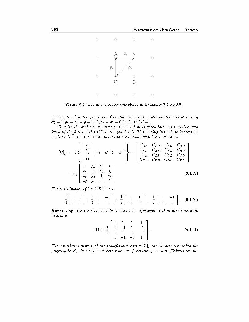
292 Waveform-Based Video Coding Chapter 9
A B
C D
�h
�v �d
Figure 9.6. The image source considered in Examples 9.4,9.5,9.6.
using optimal scalar quantizer. Give the numerical results for the special case of
�2s = 1; �h = �v = � = 0:95; �d = �2 = 0:9025; and R = 2:
To solve the problem, we arrange the 2 � 2 pixel array into a 4-D vector, and
think of the 2 � 2 2-D DCT as a 4-point 1-D DCT. Using the 1-D ordering s =
[A;B;C;D]T , the covariance matrix of s is, assuming s has zero mean,
[C]s = E
8>><>>:
2664A
B
C
D
3775 [ A B C D ]
9>>=>>; =
2664CAA CAB CAC CADCBA CBB CBC CBDCCA CCB CCC CCDCDA CDB CDC CDD
3775
= �2s
2664
1 �h �v �d�h 1 �d �v�v �d 1 �h�d �v �h 1
3775 : (9.1.49)
The basis images of 2� 2 DCT are:
1
2
�1 1
1 1
�;
1
2
�1 �11 �1
�;
1
2
�1 1
�1 �1�;
1
2
�1 �1�1 1
�: (9.1.50)
Rearranging each basis image into a vector, the equivalent 1-D inverse transform
matrix is
[U] =1
2
2664
1 1 1 1
1 �1 1 �11 1 �1 �11 �1 �1 1
3775 : (9.1.51)
The covariance matrix of the transformed vector [C]t can be obtained using the
property in Eq. (9.1.12), and the variances of the transformed coeÆcients are the
Section 9.1. Block-Based Transform Coding 293
diagonal element in [C]t. In the special case of �h = �v = � = 0:95; �d = �2 =
0:9025; the coeÆcient variances are
�2t;k = f(1 + �)2; (1� �2); (1� �2); (1� �)2g�2s (9.1.52)
= f3:8025; 0:0975; 0:0975; 0:0025g: (9.1.53)
The geometric mean of the coeÆcient variances is
�2t =
Yk
�2t;k
!1=4
= (1� �2)�2s = 0:0975: (9.1.54)
If the desired average bit rate is R = 2 bit/pixel (bpp), the optimal bit allocation
among the 4 coeÆcients are, using Eq. (9.1.43):
Rk = f4:64; 2; 2;�0:64g: (9.1.55)
The average distortion per pixel is, using Eq. (9.1.44) and �2t;k = �2Gaussian,
DTC = �2Gaussian(1� �2)�2s2�2R = 0:0061�2Gaussian (9.1.56)
If one directly quantizes each pixel, then the average distortion (assuming opti-
mal quantizer) is, using Eq. (9.1.45)
DPCM = �2Gaussian�2s2�2R = 0:0625�2Gaussian (9.1.57)
The transform coding gain is, using Eq. (9.1.48)
GTC =�2s�2t
=1
1� �2= 10:25: (9.1.58)
Notice that the optimal bit allocation in Eq. (9.1.55) assumes that one can code
a variable using a negative number of bits. In practice, one must set R4 = 0, and
reallocate the total number of bits among the remaining three variables. A simple
solution is to set R1 = 4, so that the modi�ed bit allocation is
Rk = f4; 2; 2; 0g: (9.1.59)
The average distortion in this case is
Dt =1
4
Xk
�2Gaussian�2t;k2
�2Rk = 0:0074�2Gaussian: (9.1.60)
Although this distortion is higher than that indicated by Eq. (9.1.56), it is still much
lower than that achievable by PCM.
294 Waveform-Based Video Coding Chapter 9
9.1.6 Optimal Transform Design and the KLT
As shown above, with optimal bit allocation and optimal scalar quantization, the
transform coding yields a lower average distortion than the PCM method. This
is true with any unitary transform. It is natural then to question whether there
exists an optimal transform that will minimize the distortion Ds, or equivalently
maximize the gain GTC. Because �2s�2s is �xed for a given source, the transform
should be such that it yields the minimal geometric mean�Q
k �2t;k�
2t;k
�1=N, among
all N�N unitary transforms. Fortunately, when the source is Gaussian, the answer
is a de�nite \yes", and such an optimal transform is the KLT.
Construction of the KLT Bases
With the KLT, the basis vectors are designed based on the covariance matrix of the
original signal [C]s. Let �k and �k represent the k-th eigenvalue and normalized
eigenvector of [C]s: Then they satisfy:
[C]s�k = �k�k; with < �k;�l >= Æk;l:
The KLT for a given covariance matrix [C]s is the one which uses �k as the basis
vectors. The corresponding inverse transform matrix is:
[�] = [�0;�1; � � � ;�N�1]: (9.1.61)
Replacing [V] in Eq. (9.1.12) by [�]H , we get
[C]t = [�]H [C]s[�] =
2664�H1
�H2
� � ��HN
3775 [C]s[�1;�2; � � � ;�N ] (9.1.62)
=
2664�H1
�H2
� � ��HN
3775 [�1�1; �2�2; � � � ; �N�N ] =
2664�1 0 � � � 0
0 �2 � � � 0
� � � � � � � � � � � �0 0 � � � �N
3775(9.1.63)
That is, the KLT diagonalizes [C]s: Further, the variance of the k-th transformed
coeÆcient is �2k = Ct(k; k) = �k :
To prove that the KLT will minimize the coding distortion, we make use of the
inequality
det[C] �Yk2N
�2t;k (9.1.64)
which applies to any covariance matrix [C] with diagonal entries �2t;k . On the other
hand, from Eq. (9.1.12), we have
det[C]t = det[C]s (9.1.65)
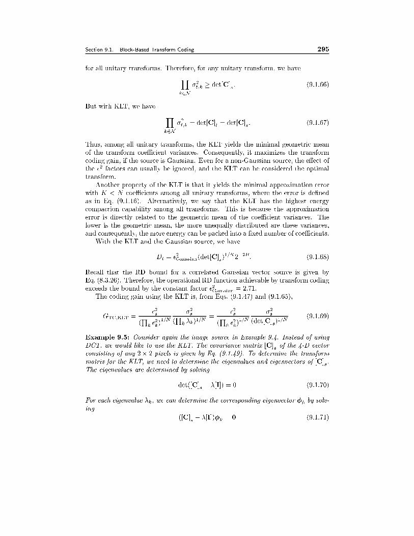
Section 9.1. Block-Based Transform Coding 295
for all unitary transforms. Therefore, for any unitary transform, we haveYk2N
�2t;k � det[C]s: (9.1.66)
But with KLT, we have Yk2N
�2t;k = det[C]t = det[C]s: (9.1.67)
Thus, among all unitary transforms, the KLT yields the minimal geometric mean
of the transform coeÆcient variances. Consequently, it maximizes the transform
coding gain, if the source is Gaussian. Even for a non-Gaussian source, the e�ect of
the �2 factors can usually be ignored, and the KLT can be considered the optimal
transform.
Another property of the KLT is that it yields the minimal approximation error
with K < N coeÆcients among all unitary transforms, where the error is de�ned
as in Eq. (9.1.16). Alternatively, we say that the KLT has the highest energy
compaction capability among all transforms. This is because the approximation
error is directly related to the geometric mean of the coeÆcient variances. The
lower is the geometric mean, the more unequally distributed are these variances,
and consequently, the more energy can be packed into a �xed number of coeÆcients.
With the KLT and the Gaussian source, we have
Dt = �2Gaussian(det[C]s)1=N2�2R: (9.1.68)
Recall that the RD bound for a correlated Gaussian vector source is given by
Eq. (8.3.26). Therefore, the operational RD function achievable by transform coding
exceeds the bound by the constant factor �2Gaussian = 2:71:
The coding gain using the KLT is, from Eqs. (9.1.47) and (9.1.65),
GTC;KLT =�2s
(Qk �
2k)1=N
�2s
(Qk �k)
1=N=
�2s
(Qk �
2k)1=N
�2s
(det[C]s)1=N
(9.1.69)
Example 9.5: Consider again the image source in Example 9.4. Instead of using
DCT, we would like to use the KLT. The covariance matrix [C]s of the 4-D vector
consisting of any 2� 2 pixels is given by Eq. (9.1.49). To determine the transform
matrix for the KLT, we need to determine the eigenvalues and eigenvectors of [C]s.
The eigenvalues are determined by solving
det([C]s � �[I]) = 0 (9.1.70)
For each eigenvalue �k, we can determine the corresponding eigenvector �k by solv-
ing
([C]s � �[I])�k = 0 (9.1.71)
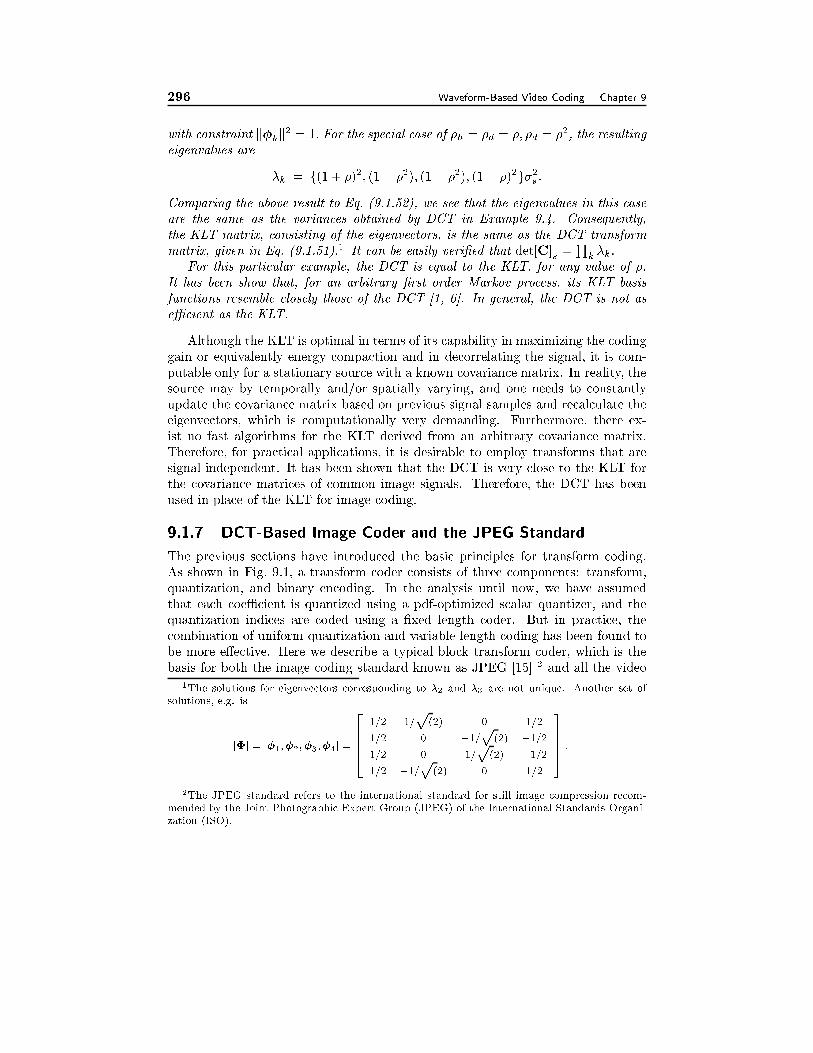
296 Waveform-Based Video Coding Chapter 9
with constraint k�kk2 = 1: For the special case of �h = �d = �; �d = �2, the resulting
eigenvalues are
�k = f(1 + �)2; (1� �2); (1� �2); (1� �)2g�2s :Comparing the above result to Eq. (9.1.52), we see that the eigenvalues in this case
are the same as the variances obtained by DCT in Example 9.4. Consequently,
the KLT matrix, consisting of the eigenvectors, is the same as the DCT transform
matrix, given in Eq. (9.1.51).1 It can be easily veri�ed that det[C]s =Qk �k :
For this particular example, the DCT is equal to the KLT, for any value of �.
It has been show that, for an arbitrary �rst order Markov process, its KLT basis
functions resemble closely those of the DCT [1, 6]. In general, the DCT is not as
eÆcient as the KLT.
Although the KLT is optimal in terms of its capability in maximizing the coding
gain or equivalently energy compaction and in decorrelating the signal, it is com-
putable only for a stationary source with a known covariance matrix. In reality, the
source may by temporally and/or spatially varying, and one needs to constantly
update the covariance matrix based on previous signal samples and recalculate the
eigenvectors, which is computationally very demanding. Furthermore, there ex-
ist no fast algorithms for the KLT derived from an arbitrary covariance matrix.
Therefore, for practical applications, it is desirable to employ transforms that are
signal-independent. It has been shown that the DCT is very close to the KLT for
the covariance matrices of common image signals. Therefore, the DCT has been
used in place of the KLT for image coding.
9.1.7 DCT-Based Image Coder and the JPEG Standard
The previous sections have introduced the basic principles for transform coding.
As shown in Fig. 9.1, a transform coder consists of three components: transform,
quantization, and binary encoding. In the analysis until now, we have assumed
that each coeÆcient is quantized using a pdf-optimized scalar quantizer, and the
quantization indices are coded using a �xed length coder. But in practice, the
combination of uniform quantization and variable length coding has been found to
be more e�ective. Here we describe a typical block transform coder, which is the
basis for both the image coding standard known as JPEG [15] 2 and all the video
1The solutions for eigenvectors corresponding to �2 and �3 are not unique. Another set of
solutions, e.g. is
[�] = [�1;�2;�3;�4] =
2664
1=2 1=p
(2) 0 1=2
1=2 0 �1=p
(2) �1=2
1=2 0 1=p
(2) �1=2
1=2 �1=p
(2) 0 1=2
3775 :
2The JPEG standard refers to the international standard for still image compression recom-
mended by the Joint Photographic Expert Group (JPEG) of the International Standards Organi-
zation (ISO).
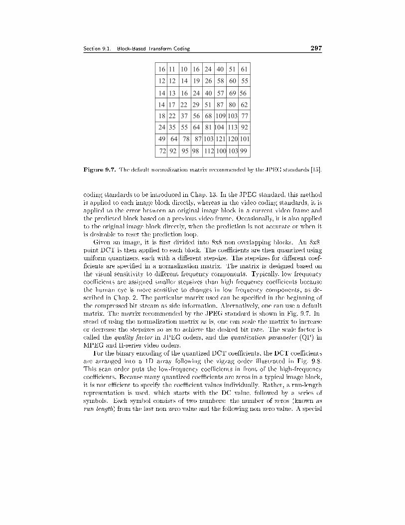
Section 9.1. Block-Based Transform Coding 297
16 11 10 16 24 40 51 61
12 12 14 19 26 58 60 55
14 13 16 24 40 57 69 56
14 17 22 29 51 87 80 62
18 22 37 56 68 109 103 77
24 35 55 64 81 104 113 92
49 64 78 87 103 121 120 101
72 92 95 98 112 100 103 99
Figure 9.7. The default normalization matrix recommended by the JPEG standards [15].
coding standards to be introduced in Chap. 13. In the JPEG standard, this method
is applied to each image block directly, whereas in the video coding standards, it is
applied to the error between an original image block in a current video frame and
the predicted block based on a previous video frame. Occasionally, it is also applied
to the original image block directly, when the prediction is not accurate or when it
is desirable to reset the prediction loop.
Given an image, it is �rst divided into 8x8 non-overlapping blocks. An 8x8-
point DCT is then applied to each block. The coeÆcients are then quantized using
uniform quantizers, each with a di�erent stepsize. The stepsizes for di�erent coef-
�cients are speci�ed in a normalization matrix. The matrix is designed based on
the visual sensitivity to di�erent frequency components. Typically, low frequency
coeÆcients are assigned smaller stepsizes than high frequency coeÆcients because
the human eye is more sensitive to changes in low frequency components, as de-
scribed in Chap. 2. The particular matrix used can be speci�ed in the beginning of
the compressed bit stream as side information. Alternatively, one can use a default
matrix. The matrix recommended by the JPEG standard is shown in Fig. 9.7. In-
stead of using the normalization matrix as is, one can scale the matrix to increase
or decrease the stepsizes so as to achieve the desired bit rate. The scale factor is
called the quality factor in JPEG coders, and the quantization parameter (QP) in
MPEG and H-series video coders.
For the binary encoding of the quantized DCT coeÆcients, the DCT coeÆcients
are arranged into a 1D array following the zigzag order illustrated in Fig. 9.8.
This scan order puts the low-frequency coeÆcients in front of the high-frequency
coeÆcients. Because many quantized coeÆcients are zeros in a typical image block,
it is not eÆcient to specify the coeÆcient values individually. Rather, a run-length
representation is used, which starts with the DC value, followed by a series of
symbols. Each symbol consists of two numbers: the number of zeros (known as
run-length) from the last non-zero value and the following non-zero value. A special
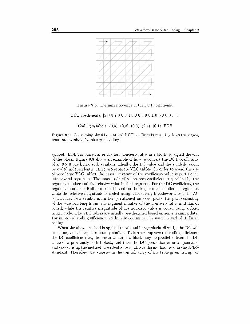
298 Waveform-Based Video Coding Chapter 9
Figure 9.8. The zigzag ordering of the DCT coeÆcients.
DCT coeÆcients: [5 0 0 2 3 0 0 4 0 0 0 0 0 0 1 0 0 0 0 0 ....0]
Coding symbols: (0,5), (2,2), (0,3), (2,4), (6,1), EOB
Figure 9.9. Converting the 64 quantized DCT coeÆcients resulting from the zigzag
scan into symbols for binary encoding.
symbol, `EOB', is placed after the last non-zero value in a block, to signal the end
of the block. Figure 9.9 shows an example of how to convert the DCT coeÆcients
of an 8� 8 block into such symbols. Ideally, the DC value and the symbols would
be coded independently using two separate VLC tables. In order to avoid the use
of very large VLC tables, the dynamic range of the coeÆcient value is partitioned
into several segments. The magnitude of a non-zero coeÆcient is speci�ed by the
segment number and the relative value in that segment. For the DC coeÆcient, the
segment number is Hu�man coded based on the frequencies of di�erent segments,
while the relative magnitude is coded using a �xed length codeword. For the AC
coeÆcients, each symbol is further partitioned into two parts, the part consisting
of the zero run-length and the segment number of the non-zero value is Hu�man
coded, while the relative magnitude of the non-zero value is coded using a �xed
length code. The VLC tables are usually pre-designed based on some training data.
For improved coding eÆciency, arithmetic coding can be used instead of Hu�man
coding.
When the above method is applied to original image blocks directly, the DC val-
ues of adjacent blocks are usually similar. To further improve the coding eÆciency,
the DC coeÆcient (i.e., the mean value) of a block may be predicted from the DC
value of a previously coded block, and then the DC prediction error is quantized
and coded using the method described above. This is the method used in the JPEG
standard. Therefore, the stepsize in the top-left entry of the table given in Fig. 9.7
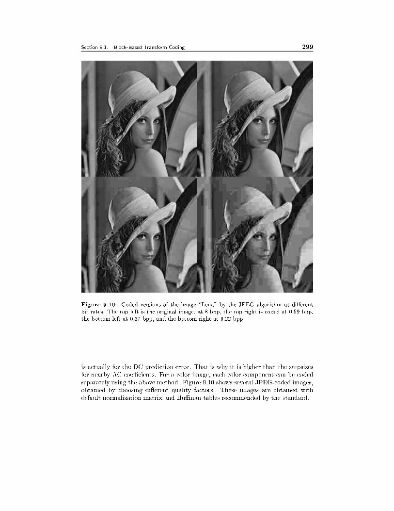
Section 9.1. Block-Based Transform Coding 299
Figure 9.10. Coded versions of the image \Lena" by the JPEG algorithm at di�erent
bit rates. The top left is the original image, at 8 bpp, the top right is coded at 0.59 bpp,
the bottom left at 0.37 bpp, and the bottom right at 0.22 bpp.
is actually for the DC prediction error. That is why it is higher than the stepsizes
for nearby AC coeÆcients. For a color image, each color component can be coded
separately using the above method. Figure 9.10 shows several JPEG-coded images,
obtained by choosing di�erent quality factors. These images are obtained with
default normalization matrix and Hu�man tables recommended by the standard.
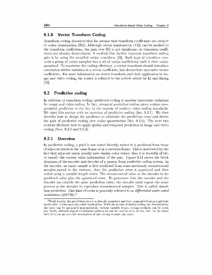
300 Waveform-Based Video Coding Chapter 9
9.1.8 Vector Transform Coding
Transform coding discussed thus far assume that transform coeÆcients are subject
to scalar quantization (SQ). Although vector quantization (VQ) can be applied to
the transform coeÆcients, the gain over SQ is not signi�cant, as transform coeÆ-
cients are already decorrelated. A method that further improves transform coding
gain is by using the so-called vector transform [22]. Such type of transform con-
verts a group of vector samples into a set of vector coeÆcients, each is then vector
quantized. To maximize the coding eÆciency, a vector transform should introduce
correlation within variables in a vector coeÆcient, but decorrelate successive vector
coeÆcients. For more information on vector transform and their application in im-
age and video coding, the reader is referred to the review article by Li and Zhang
[23].
9.2 Predictive coding
In addition to transform coding, predictive coding is another important technique
for image and video coding. In fact, temporal predictive coding using motion com-
pensated prediction is the key to the success of modern video coding standards.
We start this section with an overview of predictive coding (Sec. 9.2.1). We then
describe how to design the predictor to minimize the prediction error and derive
the gain of predictive coding over scalar quantization (Sec. 9.2.2). The next two
sections illustrate how to apply spatial and temporal prediction in image and video
coding (Secs. 9.2.3 and 9.2.4).
9.2.1 Overview
In predictive coding, a pixel is not coded directly, rather it is predicted from those
of adjacent pixels in the same frame or in a previous frame. This is motivated by the
fact that adjacent pixels usually have similar color values, thus it is wasteful of bits
to specify the current value independent of the past. Figure 9.11 shows the block
diagrams of the encoder and decoder of a generic lossy predictive coding system. In
the encoder, an input sample is �rst predicted from some previously reconstructed
samples stored in the memory, then the prediction error is quantized and then
coded using a variable length coder. The reconstructed value at the decoder is the
predicted value plus the quantized error. To guarantee that the encoder and the
decoder use exactly the same prediction value, the encoder must repeat the same
process as the decoder to reproduce reconstructed samples. This is called closed-
loop prediction. This kind of coder is generally referred to as di�erential pulse coded
modulation (DPCM).3
3Traditionally, the prediction error is uniformly quantized and then transmitted using amplitude
modulation known as pulse coded modulation. With the advent of digital coding and transmission,
the error can be quantized non-uniformly, various variable length coding methods can be used,
and �nally di�erent digital modulation techniques can be used to carry binary bits. So the name
DPCM is not an accurate description of this coding scheme any more.
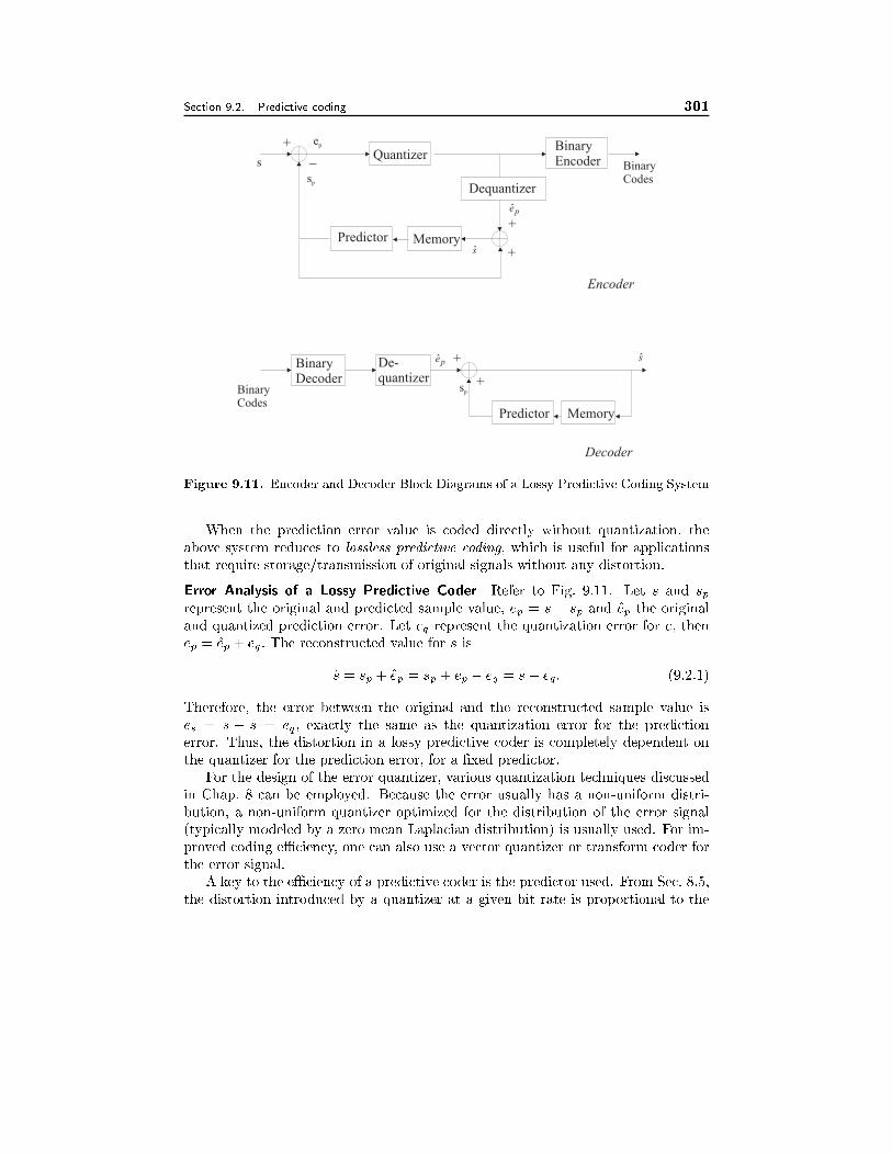
Section 9.2. Predictive coding 301
BinaryEncoder
Predictor Memory
Quantizer
Dequantizer
+
+
+
_
+
+
sp
sp
ep
BinaryDecoder
De-quantizer
Predictor Memory
BinaryCodes
BinaryCodes
Encoder
Decoder
s
s
s
pe
pe
Figure 9.11. Encoder and Decoder Block Diagrams of a Lossy Predictive Coding System
When the prediction error value is coded directly without quantization, the
above system reduces to lossless predictive coding, which is useful for applications
that require storage/transmission of original signals without any distortion.
Error Analysis of a Lossy Predictive Coder Refer to Fig. 9.11. Let s and sprepresent the original and predicted sample value, ep = s � sp and ep the original
and quantized prediction error. Let eq represent the quantization error for e, then
ep = ep + eq : The reconstructed value for s is
s = sp + ep = sp + ep � eq = s� eq: (9.2.1)
Therefore, the error between the original and the reconstructed sample value is
es = s � s = eq ; exactly the same as the quantization error for the prediction
error. Thus, the distortion in a lossy predictive coder is completely dependent on
the quantizer for the prediction error, for a �xed predictor.
For the design of the error quantizer, various quantization techniques discussed
in Chap. 8 can be employed. Because the error usually has a non-uniform distri-
bution, a non-uniform quantizer optimized for the distribution of the error signal
(typically modeled by a zero mean Laplacian distribution) is usually used. For im-
proved coding eÆciency, one can also use a vector quantizer or transform coder for
the error signal.
A key to the eÆciency of a predictive coder is the predictor used. From Sec. 8.5,
the distortion introduced by a quantizer at a given bit rate is proportional to the
302 Waveform-Based Video Coding Chapter 9
variance of the signal (cf. Eq. (8.5.18)). To maximize the coding eÆciency, the
predictor should minimize the prediction error variance. How to design a predictor
to achieve this objective is the topic of the next subsection.
9.2.2 Optimal Predictor Design and Predictive Coding Gain
In general, one can use various kinds of predictors, linear or non-linear. But in
practice, linear predictors are used almost exclusively for the ease of implementation.
Let s0 represent the current pixel, and sk; k = 1; 2; : : : ;K the previous pixels that
are used to predict s0. In a linear predictor, the predicted value for s0 is described
by
sp =
KXk=1
aksk (9.2.2)
where ak are called prediction coeÆcients. The number of samples used for pre-
diction, K, is usually called the predictor order. The key problem in designing
a predictive coder is how to determine these coeÆcients. As described before, to
maximize the coding eÆciency, one should minimize the variance of the prediction
error, which is equivalent to the MSE of the predictor. Letting Sk represent the RVcorresponding to sk, and Sp the RV corresponding to sp; this error is de�ned as:
�2p = EfjS0 � Spj2g = EfjS0 �KXk=1
akSkj2g: (9.2.3)
The optimal prediction coeÆcients should minimize the above error. This can be
accomplished by letting@�2p@al
= 0, which yields
Ef(S0 �KXk=1
akSk)Slg = 0; l = 1; 2 : : : ;K: (9.2.4)
Note that the above equation is precisely the orthogonality principle for linear min-
imal mean square error (LMMSE) estimator. It says that the prediction error must
be orthogonal to each past sample used for prediction. Let R(k; l) = EfSkSlg rep-resent the correlation between Sk and Sl: From Eq. (9.2.4), one can easily derive
the following set of linear equations
KXk=1
akR(k; l) = R(0; l); l = 1; 2 : : : ;K; (9.2.5)
or in matrix form2664
R(1; 1) R(2; 1) � � � R(K; 1)
R(1; 2) R(2; 2) � � � R(K; 2)
� � � � � � � � � � � �R(1;K) R(2;K) � � � R(K;K)
37752664
a1a2� � �aK
3775 =
2664
R(0; 1)
R(0; 2)
� � �R(0;K)
3775 (9.2.6)
Section 9.2. Predictive coding 303
or
[R]a = r: (9.2.7)
The above equation for solving the LMMSE predictor is usually called the Yuler-
Walker equation.
From (9.2.7), the optimal prediction coeÆcients are:
a = [R]�1r: (9.2.8)
The MSE of this predictor is:
�2p = Ef(S0 � Sp)S0g = R(0; 0)�KXk=0
akR(k; 0) (9.2.9)
= R(0; 0)� rTa = R(0; 0)� rTR�1r: (9.2.10)
The �rst equality results from (9.2.4), the orthogonality principle.
For a stationary source, the autocorrelation of a pixel is a constant, independent
of its spatial location, i.e., R(l; l) = R(0; 0); l = 1; 2; : : : ;K. Furthermore, the
correlation between two pixels are symmetrical, i.e, R(k; l) = R(l; k). The matrix R
is in fact the autocorrelation matrix of the prediction vector Sp = [S1;S2; : : : ;SK ]T ;and r = EfS0Sg is the correlation between the current pixel S0 with Sp:When the
source is a 1-D stationary source, S0 = S(n) is an arbitrary sample of the source,
and Sk = S(n � k) are the k-th previous sample from S(n), we have R(k; l) =
EfS(n � k)S(n � l)g = Rs(k � l), the correlation between two samples separated
by k � l. In this case, the matrix [R] is Toeplitz in that all the entries on the same
diagonal line are identical, and the corresponding upper and lower triangle lines
are conjugate of each other. Such a matrix can be inverted eÆciently using the
Levinson-Durbin Algorithm [29]. When the source is 2-D, the matrix [R] in general
does not have such nice structure. But only a limited number of past samples is
typically used for prediction, as the correlation between two pixels decreases rapidly
as their distance increases. Usually, at most four pixels, on the left, top, top left,
and top right of the current one, are used for prediction. In this case, direct solution
of the above equation is a simple task.
The above solution for the optimal predictor assumes that the predicted value
sp is obtained from original past samples sk. In a lossy predictive coder, sk have
to be replaced by reconstructed past samples sk: Ideally, the error in Eq. (9.2.3)
should be replaced by
�2p = EfjS0 �Xk
akSkj2g (9.2.11)
But because sk is dependent on the predictor and the quantizer in a complicated
relation, �nding a solution that minimizes the above error is very diÆcult. In
practice, one simply assumes that the quantization error is negligible and design
the predictor by minimizing the error in Eq. (9.2.3).
304 Waveform-Based Video Coding Chapter 9
Predictive Coding Gain
As with transform coding, we can de�ne the gain of predictive coding over PCM as
the ratio of the distortions incurred by the two types of coders under the same bit
rate. Recall that with predictive coding, it is the prediction error that is quantized
and coded, and that the distortion on the original signal is equal to the quantization
error for prediction error. Assuming optimal scalar quantization for the prediction
error, the distortion is related to the rate by
DDPCM = �2p�2p2�2R (9.2.12)
where �2p depends on the pdf of the prediction error, �2p is variance of the prediction
error, which is equal to the MSE of the predictor. On the other hand, the distortion-
rate function of PCM is given by Eq. (9.1.45). Therefore, the predictive coding gain
is
GDPCM =DPCM
DDPCM
=�2s�2p
�2s�2p
(9.2.13)
In general, the prediction error �2p reduces as the predictor order K increases.
With the LMMSE predictor given by Eq. (9.2.8), it can be shown [19] that the
minimal prediction error when the predictor order goes to in�nity is related to the
power spectrum of the signal S(ej!) by
�2p;min = limK!1
�2p = exp
�1
2�
Z �
��
loge S(ej!)d!
�: (9.2.14)
The ratio s =�2p;min
�2sis called the spectral atness measure of a signal. The pre-
dictive coding gain is thus inversely proportional to the spectral atness. This is
because a signal with narrowly concentrated spectrum is more amenable to predic-
tion. A signal with at spectrum (i.e., white noise) is unpredictable.
It can be shown that the integral in Eq. (9.2.14) can be written as [19]
�2p;min = limK!1
Yk
�k
!1=N
; (9.2.15)
where �k is the k-th eigenvalue of the N -th order covariance matrix of the signal.4
On the other hand, the signal variance equals
�2s = limK!1
1
K
Xk
�k (9.2.16)
Therefore, the predictive coding gain when K !1 can be expressed as
limK!1
GDPCM =�2s�2p
limK!11K
Pk �k
limK!1 (Qk �k)
K; (9.2.17)
4It can be shown that �k = S(ej!k ), where !k are in general non-equidistant samples over the
interval (��; �).
Section 9.2. Predictive coding 305
which is equal to the transform coding gain achievable with the KLT (cf. Eq. (9.1.47)),
when the transform length N goes to in�nity. Therefore, the two methods are equiv-
alent when the transform length and the predictor order are both in�nite. However,
for any �nite N , length N transform coding is less eÆcient than order N predictive
coding [19]. This is because a length N transform only involves N samples at a
time, whereas a predictive coder of any order has an e�ective memory that is in�nite,
because of the feedback of the quantization error in the closed-loop prediction.
9.2.3 Spatial Domain Linear Prediction
Let (m;n) represent a video frame. In spatial domain linear prediction, a current
pixel (m;n) is predicted from its past neighboring pixels, (k; l); (k; l) 2 B(m;n)where B(m;n) represents a causal neighborhood of pixel (m;n). The optimal predic-
tor can be determined based on Eq. (9.2.6) if the correlations between (m;n) and
each of the pixels in B(m;n) are known.Example 9.6: Consider the image source shown in Fig. 9.6 again. This time,
we use a predictive coder, which predicts the pixel s0 = (m;n) (pixel D) from
s1 = (m;n � 1) (pixel C), s2 = (m � 1; n) (pixel B), and s3 = (m � 1; n� 1)
(pixel A), as shown in Fig. 9.6. Equation (9.2.6) is reduced to, in this case:24 R(C;C) R(C;B) R(C;A)
R(B;C) R(B;B) R(B;A)
R(A;C) R(A;B) R(A;A)
3524 a1a2a3
35 =
24 R(D;C)
R(D;B)
R(D;A)
35
or 24 1 �d �v�d 1 �h�v �h 1
3524 a1a2a3
35 =
24 �h�v�d
35 :
In the special case of �h = �v = �; �d = �2, the optimal predictor is24 a1a2a3
35 =
24 �
�
��2
35 :
The MSE of the above predictor is, using Eq. (9.2.10),
�2p = R(0; 0)� � R(0; 1) R(0; 2) R(0; 3)�24 a1
a2a3
35 = (1� �2)2�2s :
With R = 2 bit optimal scalar quantization, the quantization error is
D = �2Gaussian�2p2�2R = 0:000594�2Gaussian: (9.2.18)
306 Waveform-Based Video Coding Chapter 9
The coding gain over PCM is
GDPCM =�2s�2p
=1
(1� �2)2= 105:19: (9.2.19)
Comparing the above result with those in Examples 9.4 and 9.5, we see that,
among the three methods which all involve a 2 � 2 pixel block when coding, the
predictive coding method is the most eÆcient. This is consistent with the theoretical
result, that predictive coding using an N-th order predictor is better than transform
coding with length N transform. Note that the theoretical analysis as well as the
examples all assume optimal scalar quantization, which may not be realizable in
practice. A major problem with predictive coding is that a transmission error in
the coded bit stream that a�ects a single sample can lead to mismatch between the
encoder and decoder, so that all the following reconstructed samples may be in error.
This is known as the error propagation e�ect. The e�ect of transmission errors on
coded bit streams and mechanisms to prevent or suppress such e�ect will be discussed
later (Chap. 14).
Note that spatial prediction can be applied not only to original pixel values,
but also transform coeÆcients. For example, in a block transform coder, the DC
coeÆcients (i.e., the mean values) of adjacent blocks are often similar, and one may
predict the DC value of a current block from those of the block above and to the
left. In the JPEG image coding standard discussed in Sec. 9.1.7, the left block
DC value is used for prediction. Usually, the correlation between AC coeÆcients of
adjacent blocks are not strong enough to warrant the use of prediction.
In coders using wavelet transforms (Sec. 11.3), the coeÆcients in the same spatial
position but di�erent scales are often correlated. Therefore, prediction among these
coeÆcients can also be applied. There, instead of predicting the actual coeÆcient
value, a non-linear predictor is often used, which predicts locations of non-zero
coeÆcients in a �ne scale from the locations of non-zero coeÆcients in a coarser
scale.
9.2.4 Motion Compensated Temporal Prediction
Uni-Directional Temporal Prediction
In addition to applying prediction within the same frame, one can predict a pixel
value in a current frame from its corresponding pixel in a previous frame. Let (x; t)
represent the pixel value in frame t at pixel x, and let t� denote the previous frame
time. Then the prediction process is described by
p(x; t) = (x; t�): (9.2.20)
This is known as linear temporal prediction. Such type of prediction is e�ective
only if the underlying scene is stationary. In a real-world video, the objects in the
scene as well as the camera are usually moving, so that the pixels with the same
Section 9.2. Predictive coding 307
spatial location in two adjacent frames can have very di�erent values. In this case,
motion-compensated prediction (MCP) is more appropriate, which uses
p(x; t) = (x+ d(x); t�); (9.2.21)
where d(x) represent the motion vector (MV) of pixel x from time t to t�. Using
the terminology introduced in Chap. 6, frame t is the anchor frame, and frame t�is the tracked frame. In video coding literature, frame t� is usually referred to as
the reference frame, and frame t the coded frame or current frame, and p(x; t) is
called the predicted frame. The reference frame must be coded and reconstructed
before the coded frame.
In a coder using MCP, both the MV and the prediction error need to be speci�ed.
Obviously, if one speci�es a MV at every pixel plus a prediction error value, one may
have to use more bits than specifying the original pixel value for each pixel. In a real
coder, more compact motion representation is used to reduce the bit rate for coding
the motion. One popular video coding method is to use the block-based motion
representation, and code only one MV per block. We will discuss block-based video
coders in Sec. 9.3.
The temporal predictors introduced thus far only use one pixel in a previous
frame. This restriction results mainly from a practical implementation constraint,
where storage of more than one previous frame is often too costly. Theoretically,
however, using pixels from more than one previous frame can improve prediction
accuracy. In this case, one can still use the optimal predictor design solution given in
Eq. (9.2.6) to determine the predictor coeÆcients associated with di�erent previous
pixels.
Bi-Directional Temporal Prediction
In fact, the predictor does not have to rely on pixels in previous frames only. In bi-
directional temporal prediction, a pixel in a current frame is predicted from a pixel
in a previous frame t� as well as a pixel in a following frame t+. The predicted
value at frame t is described by
p(x; t) = a� (x + d�(x); t�) + a+ (x+ d+(x); t+) (9.2.22)
where d�(x) and d+(x) represent the MV at x from t to t� and that from t to
t+. Typically, we call the prediction of the current frame from a previous (t� < t)
reference frame forward motion compensation, and that from a future (t� > t)
reference frame backward motion compensation.5 Ideally, coeÆcients a� and a+should be determined using the optimal predictor solution given in Eq. (9.2.6),
which requires the knowledge of the correlation between corresponding pixels in the
three frames involved. In practice, they are typically chosen heuristically. For the
predicted value to have the same mean value as the original value, they are chosen
so that a� + a+ = 1:
5This should not be confused with the backward and forward motion estimation de�ned previ-
ously in Sec. 6.2.
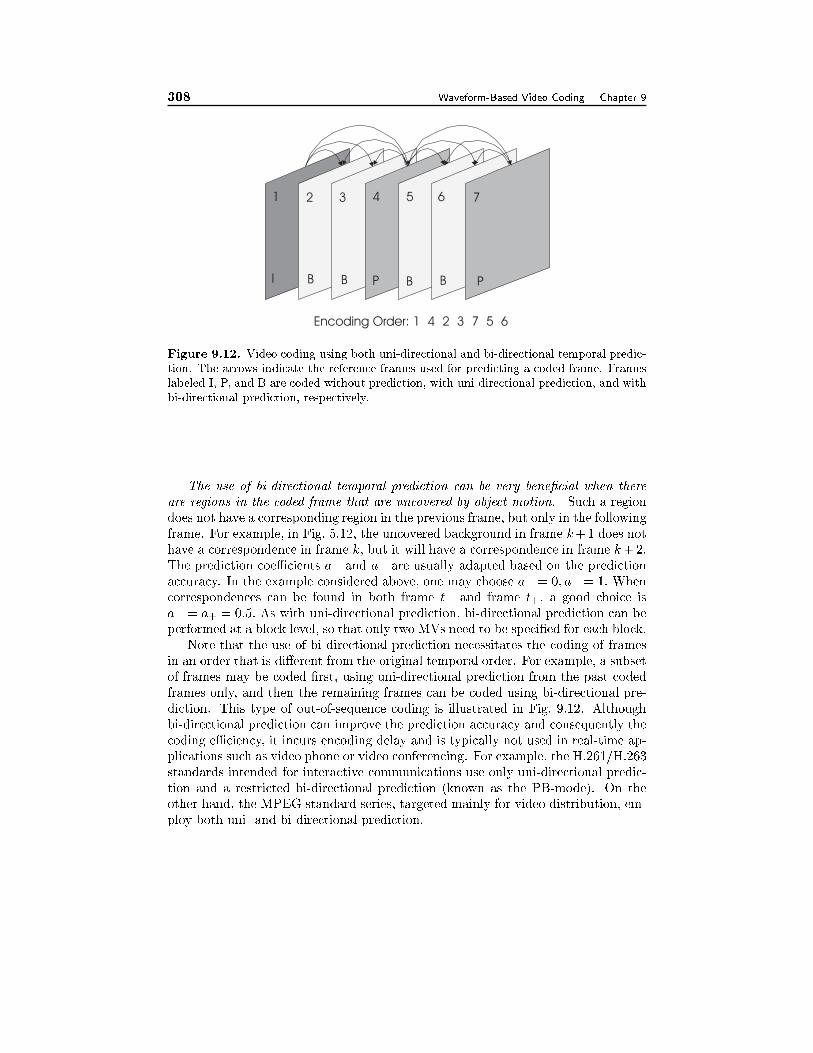
308 Waveform-Based Video Coding Chapter 9
I
I B B P B B P
Encoding Order: 1 4 2 3 7 5 6
1 2 3 4 5 6 7
Figure 9.12. Video coding using both uni-directional and bi-directional temporal predic-
tion. The arrows indicate the reference frames used for predicting a coded frame. Frames
labeled I, P, and B are coded without prediction, with uni-directional prediction, and with
bi-directional prediction, respectively.
The use of bi-directional temporal prediction can be very bene�cial when there
are regions in the coded frame that are uncovered by object motion. Such a region
does not have a corresponding region in the previous frame, but only in the following
frame. For example, in Fig. 5.12, the uncovered background in frame k+1 does not
have a correspondence in frame k, but it will have a correspondence in frame k+2:
The prediction coeÆcients a� and a+ are usually adapted based on the prediction
accuracy. In the example considered above, one may choose a� = 0; a+ = 1: When
correspondences can be found in both frame t� and frame t+, a good choice is
a� = a+ = 0:5: As with uni-directional prediction, bi-directional prediction can be
performed at a block level, so that only two MVs need to be speci�ed for each block.
Note that the use of bi-directional prediction necessitates the coding of frames
in an order that is di�erent from the original temporal order. For example, a subset
of frames may be coded �rst, using uni-directional prediction from the past coded
frames only, and then the remaining frames can be coded using bi-directional pre-
diction. This type of out-of-sequence coding is illustrated in Fig. 9.12. Although
bi-directional prediction can improve the prediction accuracy and consequently the
coding eÆciency, it incurs encoding delay and is typically not used in real-time ap-
plications such as video phone or video conferencing. For example, the H.261/H.263
standards intended for interactive communications use only uni-directional predic-
tion and a restricted bi-directional prediction (known as the PB-mode). On the
other hand, the MPEG standard series, targeted mainly for video distribution, em-
ploy both uni- and bi-directional prediction.
Section 9.3. Video Coding Using Temporal Prediction and Transform 309
9.3 Video Coding Using Temporal Prediction and Transform
A popular and e�ective video coding method is the one that uses block-based tem-
poral prediction and transform coding. This method is essentially the core of all the
international video coding standards. In this section, we �rst provide an overview
of this coding method (Sec. 9.3.1). This will be followed by its extension that uses
more sophisticated motion-compensated prediction (Sec. 9.3.2) and loop �ltering
(Sec. 9.3.5). As an optional advanced topic, we analyze the in uence of motion
estimation accuracy and loop �lter on the coding eÆciency (Sec. 9.3.5). Finally,
we consider the issue of how to choose various coding parameters in this coding
method to maximize the coding eÆciency under the rate constraint imposed by the
underlying application (Secs. 9.3.3 and 9.3.4).
9.3.1 Block-Based Hybrid Video Coding
In this coder, each video frame is divided into blocks of a �xed size and each block is
more or less processed independently, hence the name \block-based". The word \hy-
brid" means that each block is coded using a combination of motion-compensated
temporal prediction and transform coding. Figure 9.13 shows the key steps in this
coding paradigm. First, a block is predicted from a previously coded reference
frame using block-based motion estimation. The motion vector (MV) speci�es the
displacement between the current block and the best matching block. The pre-
dicted block is obtained from the previous frame based on the estimated MV using
motion compensation.6 Then, the prediction error block is coded, by transforming
it using the DCT, quantizing the DCT coeÆcients, and converting them into binary
codewords using variable length coding (VLC). The actual coding method follows
that described in Sec. 9.1.7.7 As with the JPEG standard, the quantization of the
DCT coeÆcients is controlled by a quantization parameter (QP)8, which scales a
pre-de�ned quantization matrix. A larger QP corresponds to large quantization
stepsizes. Note that the encoder must emulate the decoder operation to deduce
the same reconstructed frame as the decoder, so that there will be no mismatch
between the reference frames used for prediction.
The above discussion assumes that temporal prediction is successful, in that the
prediction error block requires fewer bits to code than the original image block.
This method of coding is called P-mode. When this is not the case, the original
block will be coded directly using transform coding. This is known as intra-mode.
Instead of using a single reference frame for prediction, bi-directional prediction
can be used, which �nds two best matching blocks, one in a previous frame and
6The phrase motion compensation here and subsequently in this book refers to motion com-
pensated prediction.7Ideally, if the prediction is very accurate, then the error pattern would be close to white noise
and can be e�ectively coded using scalar quantization. In reality, however, the use of block-based
motion model often leads to structured error patterns. Transform coding is used to exploit the
correlation between error pixels.8which is called quality factor in the JPEG standard.
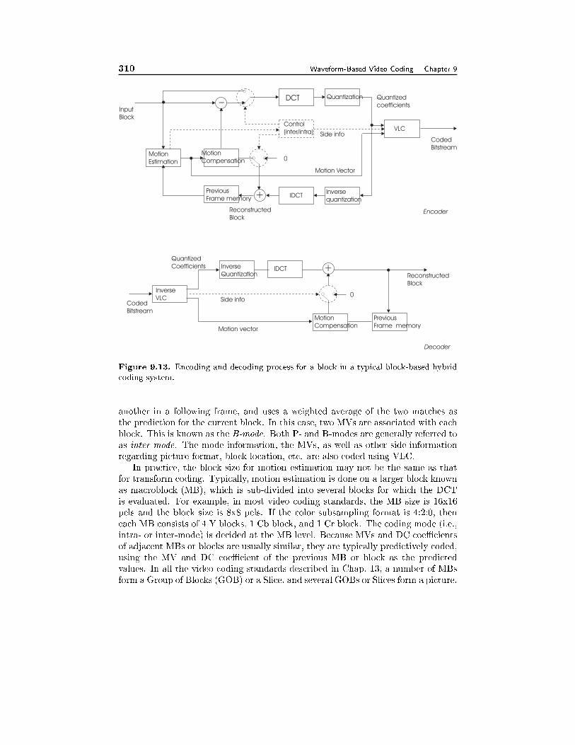
310 Waveform-Based Video Coding Chapter 9
DCT Quantization
Control(inter/intra)
VLC
MotionEstimation
MotionCompensation
PreviousFrame memory
IDCTInversequantization
_InputBlock
CodedBitstream
0
0
+
+
Quantizedcoefficients
Side info
Motion Vector
InverseVLC
InverseQuantization
IDCT
MotionCompensation
PreviousFrame memory
CodedBitstream
Motion vector
Side info
QuantizedCoefficients
ReconstructedBlock
ReconstructedBlock
Encoder
Decoder
Figure 9.13. Encoding and decoding process for a block in a typical block-based hybrid
coding system.
another in a following frame, and uses a weighted average of the two matches as
the prediction for the current block. In this case, two MVs are associated with each
block. This is known as the B-mode. Both P- and B-modes are generally referred to
as inter-mode. The mode information, the MVs, as well as other side information
regarding picture format, block location, etc. are also coded using VLC.
In practice, the block size for motion estimation may not be the same as that
for transform coding. Typically, motion estimation is done on a larger block known
as macroblock (MB), which is sub-divided into several blocks for which the DCT
is evaluated. For example, in most video coding standards, the MB size is 16x16
pels and the block size is 8x8 pels. If the color subsampling format is 4:2:0, then
each MB consists of 4 Y blocks, 1 Cb block, and 1 Cr block. The coding mode (i.e.,
intra- or inter-mode) is decided at the MB level. Because MVs and DC coeÆcients
of adjacent MBs or blocks are usually similar, they are typically predictively coded,
using the MV and DC coeÆcient of the previous MB or block as the predicted
values. In all the video coding standards described in Chap. 13, a number of MBs
form a Group of Blocks (GOB) or a Slice, and several GOBs or Slices form a picture.
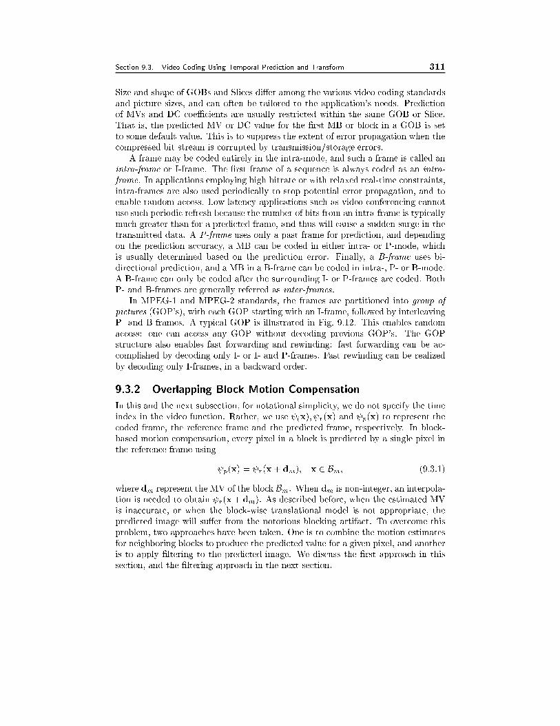
Section 9.3. Video Coding Using Temporal Prediction and Transform 311
Size and shape of GOBs and Slices di�er among the various video coding standards
and picture sizes, and can often be tailored to the application's needs. Prediction
of MVs and DC coeÆcients are usually restricted within the same GOB or Slice.
That is, the predicted MV or DC value for the �rst MB or block in a GOB is set
to some default value. This is to suppress the extent of error propagation when the
compressed bit stream is corrupted by transmission/storage errors.
A frame may be coded entirely in the intra-mode, and such a frame is called an
intra-frame or I-frame. The �rst frame of a sequence is always coded as an intra-
frame. In applications employing high bitrate or with relaxed real-time constraints,
intra-frames are also used periodically to stop potential error propagation, and to
enable random-access. Low latency applications such as video conferencing cannot
use such periodic refresh because the number of bits from an intra-frame is typically
much greater than for a predicted frame, and thus will cause a sudden surge in the
transmitted data. A P-frame uses only a past frame for prediction, and depending
on the prediction accuracy, a MB can be coded in either intra- or P-mode, which
is usually determined based on the prediction error. Finally, a B-frame uses bi-
directional prediction, and a MB in a B-frame can be coded in intra-, P- or B-mode.
A B-frame can only be coded after the surrounding I- or P-frames are coded. Both
P- and B-frames are generally referred as inter-frames.
In MPEG-1 and MPEG-2 standards, the frames are partitioned into group of
pictures (GOP's), with each GOP starting with an I-frame, followed by interleaving
P- and B-frames. A typical GOP is illustrated in Fig. 9.12. This enables random
access: one can access any GOP without decoding previous GOP's. The GOP
structure also enables fast forwarding and rewinding: fast forwarding can be ac-
complished by decoding only I- or I- and P-frames. Fast rewinding can be realized
by decoding only I-frames, in a backward order.
9.3.2 Overlapping Block Motion Compensation
In this and the next subsection, for notational simplicity, we do not specify the time
index in the video function. Rather, we use (x); r(x) and p(x) to represent the
coded frame, the reference frame and the predicted frame, respectively. In block-
based motion compensation, every pixel in a block is predicted by a single pixel in
the reference frame using
p(x) = r(x+ dm); x 2 Bm; (9.3.1)
where dm represent the MV of the block Bm. When dm is non-integer, an interpola-
tion is needed to obtain r(x+ dm). As described before, when the estimated MV
is inaccurate, or when the block-wise translational model is not appropriate, the
predicted image will su�er from the notorious blocking artifact. To overcome this
problem, two approaches have been taken. One is to combine the motion estimates
for neighboring blocks to produce the predicted value for a given pixel, and another
is to apply �ltering to the predicted image. We discuss the �rst approach in this
section, and the �ltering approach in the next section.
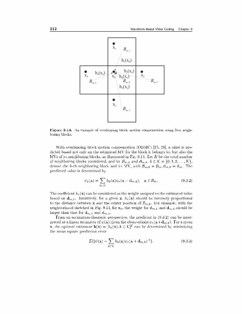
312 Waveform-Based Video Coding Chapter 9
h (x )1 0
h (x )0 0x0
x1 Bm, 1
Bm, 2
Bm, 3
Bm, 4Bm, 0
x2
x3
x4
h (x )2 0
h (x )3 0
h (x )4 0
Figure 9.14. An example of overlapping block motion compensation using four neigh-
boring blocks.
With overlapping block motion compensation (OBMC) [25, 26], a pixel is pre-
dicted based not only on the estimated MV for the block it belongs to, but also the
MVs of its neighboring blocks, as illustrated in Fig. 9.14. Let K be the total number
of neighboring blocks considered, and let Bm;k and dm;k, k 2 K = f0; 1; 2; : : : ;Kg;denote the k-th neighboring block and its MV, with Bm;0 = Bm;dm;0 = dm. The
predicted value is determined by
p(x) =Xk2K
hk(x) r(x+ dm;k); x 2 Bm: (9.3.2)
The coeÆcient hk(x) can be considered as the weight assigned to the estimated value
based on dm;k. Intuitively, for a given x, hk(x) should be inversely proportional
to the distance between x and the center position of Bm;k. For example, with the
neighborhood sketched in Fig. 9.14, for x0, the weight for dm;1 and dm;4 should be
larger than that for dm;2 and dm;3.
From an estimation-theoretic perspective, the predictor in (9.3.2) can be inter-
preted as a linear estimator of (x) given the observations r(x+dm;k). For a given
x, the optimal estimator h(x) = [hk(x); k 2 K]T can be determined by minimizing
the mean square prediction error
Efj (x)�Xk2K
hk(x) r(x + dm;k)j2g: (9.3.3)
Section 9.3. Video Coding Using Temporal Prediction and Transform 313
To preserve the mean value of the estimated image, the weights must be constrained
so that Xk2K
hk(x) = 1:
Incorporating the above constraint in the optimization by using the Lagrange mul-
tiplier method gives [26]
h(x) = R�1(x)
�r(x)� iT [R]�1(x)r(x) � 1
iT [R]�1(x)ii
�; (9.3.4)
where i is a column vector of dimension K with all elements equal to one, R and r
are the auto-correlation and cross-correlation matrices, respectively, with elements
Rk;l(x) = Ef r(x+ dm;k) r(x+ dm;l)g; k; l 2 Krk(x) = Ef (x) r(x+ dm;k)g; k 2 K:
The above solution can be used to derive the weights for di�erent neighboring
block MVs for every pixel x in a block. The expectation in the above equations is
with respect to uncertainties in both image intensity as well as motion. The above
statistics can be estimated from real video data. As indicated by the notation, they
are in general spatially variant. However, assuming (x) is stationary, the above
statistics are only dependent on the relative position of the pixel in a block, not
the absolute position with respect to the entire image. If the correlation between
pixels is symmetric, then the solution hk(x) will also be symmetric, so that only
the solution for pixels in the upper left quarter of the block need to be determined.
In general, OBMC can be applied to block MVs estimated by any method,
including the simple block matching method (BMA). However, the prediction error
can be further reduced if motion estimation is accomplished by considering OBMC.
Ideally, one should minimize the following modi�ed MCP error:Xx2Bm
j (x)�Xk2K
hk(x) r(x+ dm;k)jp (9.3.5)
Because the error for a block depends on the MVs of its adjacent blocks, one cannot
�nd one block MV at a time, as in the BMA case. One approach is to iteratively
perform motion estimation and OBMC [26]. First, the conventional BMA is used to
generate an initial set of MVs, where prediction error is calculated assuming (9.3.1)
is used for MCP. Then OBMC is applied using these motion estimates. In the next
iteration, for each block, the MV is estimated by minimizing the error given in
Eq. (9.3.5), where the MVs for the neighboring blocks are assumed to be the same
as those found in the previous iteration.
Instead of using iterations, a simpler approach is to apply non-equal weighting
to the pixels in the current block as well as neighboring blocks, when calculating the
prediction error using the BMA. To determine the proper weighting function, notice
that the MV dm of block Bm a�ects not only this block, but also its neighboring
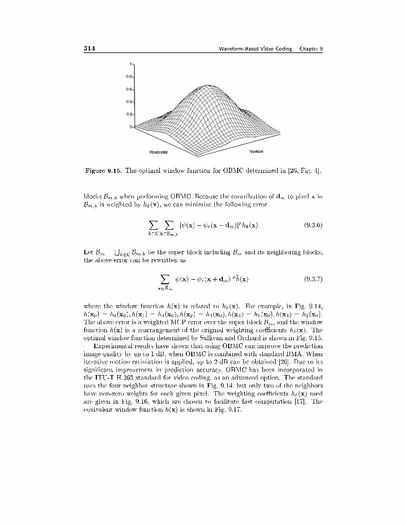
314 Waveform-Based Video Coding Chapter 9
Figure 9.15. The optimal window function for OBMC determined in [26, Fig. 4].
blocks Bm;k when performing OBMC. Because the contribution of dm to pixel x in
Bm;k is weighted by hk(x), we can minimize the following error
Xk2K
Xx2Bm;k
j (x)� r(x+ dm)jphk(x) (9.3.6)
Let �Bm =Sk2K Bm;k be the super block including Bm and its neighboring blocks,
the above error can be rewritten as
Xx2 �Bm
j (x) � r(x+ dm)jp�h(x) (9.3.7)
where the window function �h(x) is related to hk(x). For example, in Fig. 9.14,�h(x0) = h0(x0); �h(x1) = h3(x0); �h(x2) = h4(x0); �h(x3) = h1(x0); �h(x4) = h2(x0):
The above error is a weighted MCP error over the super block �Bm, and the window
function �h(x) is a rearrangement of the original weighting coeÆcients hk(x). The
optimal window function determined by Sullivan and Orchard is shown in Fig. 9.15.
Experimental results have shown that using OBMC can improve the prediction
image quality by up to 1 dB, when OBMC is combined with standard BMA. When
iterative motion estimation is applied, up to 2 dB can be obtained [26]. Due to its
signi�cant improvement in prediction accuracy, OBMC has been incorporated in
the ITU-T H.263 standard for video coding, as an advanced option. The standard
uses the four neighbor structure shown in Fig. 9.14, but only two of the neighbors
have non-zero weights for each given pixel. The weighting coeÆcients hk(x) used
are given in Fig. 9.16, which are chosen to facilitate fast computation [17]. The
equivalent window function �h(x) is shown in Fig. 9.17.
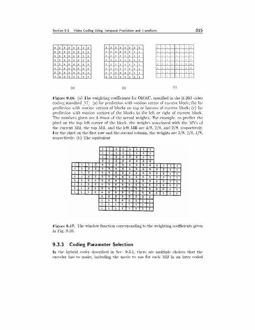
Section 9.3. Video Coding Using Temporal Prediction and Transform 315
(a) (b) (c)
Figure 9.16. (a) The weighting coeÆcients for OBMC, speci�ed in the H.263 video
coding standard [17]. (a) for prediction with motion vector of current block; (b) for
prediction with motion vectors of blocks on top or bottom of current block; (c) for
prediction with motion vectors of the blocks to the left or right of current block.
The numbers given are 8 times of the actual weights. For example, to predict the
pixel on the top left corner of the block, the weights associated with the MVs of
the current MB, the top MB, and the left MB are 4/8, 2/8, and 2/8, respectively.
For the pixel on the �rst row and the second column, the weights are 5/8, 2/8, 1/8,
respectively. (b) The equivalent
Figure 9.17. The window function corresponding to the weighting coeÆcients given
in Fig. 9.16.
9.3.3 Coding Parameter Selection
In the hybrid coder described in Sec. 9.3.1, there are multiple choices that the
encoder has to make, including the mode to use for each MB in an inter-coded
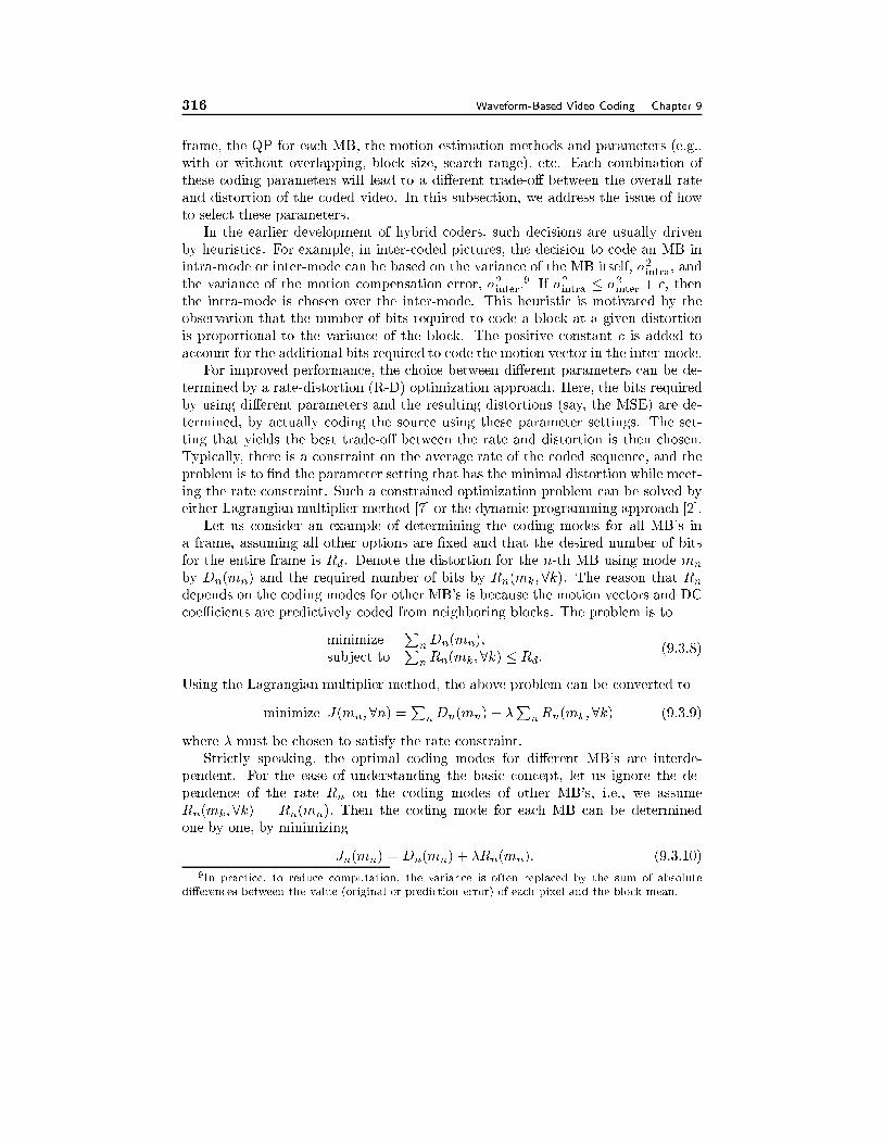
316 Waveform-Based Video Coding Chapter 9
frame, the QP for each MB, the motion estimation methods and parameters (e.g.,
with or without overlapping, block size, search range), etc. Each combination of
these coding parameters will lead to a di�erent trade-o� between the overall rate
and distortion of the coded video. In this subsection, we address the issue of how
to select these parameters.
In the earlier development of hybrid coders, such decisions are usually driven
by heuristics. For example, in inter-coded pictures, the decision to code an MB in
intra-mode or inter-mode can be based on the variance of the MB itself, �2intra, and
the variance of the motion compensation error, �2inter.9 If �2intra � �2inter + c, then
the intra-mode is chosen over the inter-mode. This heuristic is motivated by the
observation that the number of bits required to code a block at a given distortion
is proportional to the variance of the block. The positive constant c is added to
account for the additional bits required to code the motion vector in the inter-mode.
For improved performance, the choice between di�erent parameters can be de-
termined by a rate-distortion (R-D) optimization approach. Here, the bits required
by using di�erent parameters and the resulting distortions (say, the MSE) are de-
termined, by actually coding the source using these parameter settings. The set-
ting that yields the best trade-o� between the rate and distortion is then chosen.
Typically, there is a constraint on the average rate of the coded sequence, and the
problem is to �nd the parameter setting that has the minimal distortion while meet-
ing the rate constraint. Such a constrained optimization problem can be solved by
either Lagrangian multiplier method [7] or the dynamic programming approach [2].
Let us consider an example of determining the coding modes for all MB's in
a frame, assuming all other options are �xed and that the desired number of bits
for the entire frame is Rd. Denote the distortion for the n-th MB using mode mn
by Dn(mn) and the required number of bits by Rn(mk;8k). The reason that Rndepends on the coding modes for other MB's is because the motion vectors and DC
coeÆcients are predictively coded from neighboring blocks. The problem is to
minimizePnDn(mn);
subject toPnRn(mk;8k) � Rd:
(9.3.8)
Using the Lagrangian multiplier method, the above problem can be converted to
minimize J(mn;8n) =PnDn(mn) + �
PnRn(mk;8k) (9.3.9)
where � must be chosen to satisfy the rate constraint.
Strictly speaking, the optimal coding modes for di�erent MB's are interde-
pendent. For the ease of understanding the basic concept, let us ignore the de-
pendence of the rate Rn on the coding modes of other MB's, i.e., we assume
Rn(mk;8k) = Rn(mn): Then the coding mode for each MB can be determined
one by one, by minimizing
Jn(mn) = Dn(mn) + �Rn(mn): (9.3.10)
9In practice, to reduce computation, the variance is often replaced by the sum of absolute
di�erences between the value (original or prediction error) of each pixel and the block mean.
Section 9.3. Video Coding Using Temporal Prediction and Transform 317
Given that there are only a small number of possible modes to choose from, the
optimal mode for each block can be found by an exhaustive search.
Note that if mn and consequently Rn is a continuous variable, then minimizing
Jn is equivalent to setting @Jn@Rn
= 0, which leads to @Dn@Rn
= ��: This implies that
the optimal mode in each MB is such that the resulting R-D slope @Dn@Rn
is the same
among di�erent MB's.10 In practice, there are only a �nite number of modes to
choose from. Each possible mode corresponds to an operating point on a piecewise
linear R-D curve, so that each mode is associated with a range of R-D slopes. The
optimal modes for di�erent MB's found by minimizing Jn(mn) above for a given �
will have similar ranges in their R-D slopes.
The result that di�erent MB's should operate at the same R-D slope is a spe-
cial case of a variety of R-D optimization problems involving multiple independent
coding parameters. Recall that in the bit allocation problem in transform coding
(Sec. 9.1.5), the optimal solution is such that the R-D slopes for di�erent coeÆ-
cients are the same (Eq. 9.1.40). In that case, the R-D slope is proportional to
the distortion, thereby the optimal bit allocation yields identical distortion among
di�erent coeÆcients.
A diÆcult problem in the above approach is how to determine � for a given
desired rate. For an arbitrarily chosen �, the above method will yield a solution
that is optimal at a particular rate, which may or may not be close to the desired
rate. A bisection method is commonly employed to search for the � that will yield
the desired rate. A closed-form relation between � and the QP is derived in [35],
which assumes the QP is chosen based on the target bit rate (See Sec. 9.3.4).
Rate-distortion optimized selection of coding modes was �rst considered by Wie-
gand, et al. [37]. There, to handle the interdependence among the coding modes of
di�erent MB's in the same frame and over adjacent frames, a dynamic programming
scheme is employed to �nd the optimal coding modes for a set of MB's simultane-
ously. The paper by Sullivan and Wiegand [35] includes a good discussion on how to
use a similar approach to determine a variety of coding options in the H.263 coder.
It is worth noting that the R-D based approach leads to rather marginal gain over
heuristic approaches within the H.263 framework (about 10% savings in the bit rate
or 0.5 dB in PSNR) [35]. In practice, such gains may not be justi�ed considering the
quite signi�cant increase in complexity. Thus, the R-D optimized approach mainly
serves as a benchmark for evaluating the performance of a heuristic, yet practical
approach.
The computationally most demanding step in the R-D based parameter selection
approach is to collect the R-D data associated with di�erent parameter settings
(coding mode and QP and possibly di�erent motion estimation methods). This
would require actually coding all the MB's using all di�erent parameters. To reduce
10By de�nition, @Dn@Rn
= lim�R!0�D�R
, i.e., the R-D slope measures the reduction in the distor-
tion by each extra bit. The equal slope condition is equivalent to requiring all blocks operate in
such a way that an extra bit in each block will reduce the error by the same amount. Otherwise,
a block operating at a higher (resp. lower) slope should use more (resp. fewer) bits.
318 Waveform-Based Video Coding Chapter 9
the computation, some R-D models have been proposed, which relate the rate and
distortion, on the one hand, and the QP and coding modes, on the other hand
[5, 24]. Once the R-D data are obtained, one can use either Lagrangian multiplier
method or dynamic programming approach to �nd the optimal allocation. The
Lagrangian multiplier method is simpler, but has sub-optimal performance, because
it ignores interdependence between rates of adjacent MBs in the same frame or
between neighboring frames.
In addition to coding parameter selection, R-D based methods can be applied
in a variety of problems in image and video coding. One important area is motion
estimation for video coding. Whereas traditional approaches to motion estimation
focus on minimizing motion compensated prediction error only (cf. Chap. 6), R-D
optimized approaches also consider the rate needed to code the resulting MV's. For
example, the zero MV may be preferred over a non-zero MV, if it only leads to
slightly higher prediction error, considering the extra bits required to code the non-
zero MV. Furthermore, because MV's are coded in a predictive manner, smoother
motion �elds are preferred. Work on R-D optimized motion estimation can be found
in [34, 11, 20, 32, 3].
For a more complete coverage on how to use the R-D theory to optimize image
and video coding, the reader is referred to the review paper by Ortega and Ram-
chandran [28], which also contains a good exposition of Lagrangian and dynamic
programming methods as optimization tools. More extensive coverage on this topic
can be found in the book by Schuster and Katsaggelos [31].
9.3.4 Rate Control
One important issue in video coding is rate control, which refers to how to code a
video so that the resulting bitstream satis�es a target bit rate. Within the frame-
work of hybrid coding, this reduces to how to choose the coding parameters (frame
rate, inter vs. intra, QP, etc.) to meet the rate constraint. We have already alluded
to this problem in the previous subsection, where we described an R-D optimized
approach for selecting the coding mode for each MB subject to a rate constraint.
For pleasant visual perception, it is better to represent a video so that it has a
constant (or smoothly changing) quality. Because the scene activity (in terms of
motion as well as texture complexity) changes in time, the required bits will change
from frame to frame. Even if we accept changes in video quality, the bit rate cannot
be made strictly constant, due to the use of VLC and possibly di�erent coding modes
on the frame level. Therefore, the best that one can hope to achieve are constant
average rates over short intervals of time. The variability of the bit rate within each
interval has to be handled by a smoothing bu�er following the encoder. The output
bits from the encoder �rst enter the smoothing bu�er at a variable rate, and are
then moved out of the bu�er at a constant rate. The maximum time interval and
the allowed variability within this interval depend on the delay requirement of the
underlying application and the a�ordable bu�er size.11 A larger bu�er will enable
11Given the continuously diminishing cost of memory, it is reasonable to assume that the bu�er
Section 9.3. Video Coding Using Temporal Prediction and Transform 319
better video quality, but will also introduce longer delay.12
Rate control is typically accomplished in three steps:
1. Update the target average bit rate (in terms of bits/s) for each short time
interval, also referred to as rate update interval;13
2. Determine the coding mode (e.g., I, P or B-frame) and the target bit budget
for each frame to be coded in this interval, which is usually based on the target
average rate for this interval and the current bu�er fullness; and
3. Determine the coding mode and QP for each MB in a frame to meet the target
rate for this frame.
Step 1 depends on the underlying applications. For video transport over a
constant bit rate (CBR) network (such as a modem line or an ISDN channel),
the target average rate should be constant. For networks that can accommodate
variable bit rate (VBR), such as an ATM network, the coder should try to regulate
the rate to maintain a constant video quality, and yet satisfying the average and
peak rate requirement [14]. Finally, for networks where channel capacity and error
characteristics vary in time, such as the best e�ort Internet and wireless channels,
one needs to update the target average rate based on the channel conditions. The
update interval depends on how fast the network conditions change. In all these
applications, the target average bit rate per update interval should depend on not
only the available bandwidth (which would need to be estimated in time-varying
channels), but also the end-to-end delay requirement, and the current encoder bu�er
size (i.e., how many bits remain to be sent). Essentially, the target rate should be
set so that the bits from the current update interval as well as remaining bits in
the bu�er can reach the destination within the maximally allowed delay time. In
this sense, the rate constraint is determined by the delay constraint [27]. In lossy
networks, one also needs to take into account of the fact that some previously sent
data may have to be retransmitted in case they are damaged during transmission
[13]. In [27], Ortega provides a good categorization of rate control problems and
an extensive coverage on how to determine the target rate based on the underlying
network characteristics and delay requirements. For rate estimation approaches
designed for video streaming over Internet applications, see discussion in Sec. 15.3.1.
Step 2 is typically accomplished by choosing an appropriate frame rate based
on the total rate budgeted for an update interval and assigning the same target
rate for all the frames in the interval. Frames can be skipped when the bu�er
occupancy is in danger of over ow. This could happen when the bits used for
can be as large as the end-to-end delay allows, and therefore, this physical limitation of the bu�er
size can be ignored [27].12The encoder bu�er is only one factor that contributes to the end-to-end delay of a video trans-
mission. For a description of di�erent factors contributing to the end-to-end delay, see Chap. 14.13In practice, this may be done in a sliding window fashion. That is, at each new frame time,
the target bit rate for a short period of time following this frame is determined.
320 Waveform-Based Video Coding Chapter 9
the previous frames exceed the speci�ed targets by too much, or the remaining
bit budget for this interval is insuÆcient to code the video at the speci�ed frame
rate. This is the approach typically employed for interactive applications, where all
the frames, except the �rst frame, are coded in the inter-mode, so as to maintain
a fairly constant delay between frames. For broadcast or streaming of MPEG-2
coded video, an update interval usually corresponds to a GOP, which contains one
I-frame followed by interleaving P- and B-frames. Typically, rate allocation within
a GOP assumes some constant ratios between the bits used for I-, P-, and B-frames
[16]. More sophisticated, R-D based approaches would try to allocate the total
bits among frames based on the scene content, so that the average distortion is
minimized. The look-ahead involved however will incur signi�cant computations
and additional coding delay.
Rate control within a frame (i.e., step 3) can be accomplished by adjusting the
coding mode and QP for each MB, which can be done either based on some heuristic
rules or using an R-D optimized approach, as described already in Sec. 9.3.3.
The above discussions focus on video transmission applications. For storage
applications such as in DVD movies, the total bits used for a video are limited by
the capacity of the storage medium, however the bit rate may change from time to
time to accommodate changes in scene activity.
The rate control solutions discussed thus far only consider waveform-based
coders. For object-based coders such as MPEG-4, rate control must consider rate
allocation among multiple objects, and within each object, allocation among shape,
motion and texture. The frame rates of di�erent objects can also vary based on the
relative importance of each object. These problems are addressed by Vetro, et al.
[36].
Instead of producing a bit stream with a �xed target rate, another approach is
to produce a scalable bitstream, from which the receiver can choose to extract only
partial bits based on the available bandwidth. This approach is more appropriate
when the same video is to be accessed by multiple users with di�erent link capacities.
Scalable coding is discussed in Chap. 11. The distribution of a scalable stream to
users with di�erent bandwidth capacities is considered in Chap. 15.
In video coding standards, rate control is not de�ned. Instead, the encoder has
the exibility to optimize rate control as long as the coded bitstream follows the
standardized syntax. Rate control schemes used in the test models of di�erent video
coding standards will be described in Chap. 13.
A problem that is related to rate control is rate shaping. This refers to the
function of an interface (called transcoder or �lter) between the compression layer
and the network transport layer or between two network segments, with which a
pre-compressed video stream is converted so that the rate of the resulting stream
matches the available network bandwidth. This subject is discussed in Sec. 15.3.1.
Section 9.3. Video Coding Using Temporal Prediction and Transform 321
9.3.5 Loop Filtering�
The sources for motion compensated prediction error can be classi�ed into three
groups: i) the motion estimation error, ii) noise in the reference image, which can
be due to the accumulation of errors caused by motion estimation in prior frames
and quantization errors, and iii) changes in the coded frame that are not due to
motion, such as occlusion and illumination variation. In order to suppress primarily
the second source of noise, loop �ltering can be applied, which is a low-pass �lter
applied to the predicted image. Note that with non-integer motion estimates, an
interpolation �lter is used implicitly when one performs motion-compensated pre-
diction. Similarly, loop �ltering is accomplished implicitly with OBMC. However,
as can be seen below, a �lter can be speci�cally designed to reduce the e�ect of noise
in the video signal. Motion compensation with �ltering can be generally described
by
p(x; y) = g(x; y) � r(x+ dx(x; y); y + dy(x; y)); (9.3.11)
where p(x; y) represents the predicted frame, r(x; y) the reference frame, g(x; y)
the impulse response of the loop �lter, and � denotes 2-D linear convolution. In the
following, we derive the optimal �lter following the approach of Girod [10, 8, 9].
To simplify the design, the following assumptions are made: i) the reference
video frame is a stationary random �eld; ii) the errors in estimated motion vectors
at di�erent spatial positions are independent of each other; and iii) the noise term
is independent of the reference frame. With these assumptions, the power spectral
density (PSD) function of the error after motion compensated prediction can be
shown to be [8]
�e;e(fx; fy) = �s;s(fx; fy)�1 + jG(fx; fy)j2 � 2RfG(fx; fy)P (fx; fy)g
�+�n;n(fx; fy)jG(fx; fy)j2: (9.3.12)
In the above relation, �s;s(fx; fy) and �n;n(fx; fy) represent the PSD functions
of the reference frame and the noise signal, respectively, G(fx; fy) is the Fourier
transform of g(x; y), P (fx; fy) is the Fourier transform of the probability density
function (pdf) of the motion estimation error, and R denotes the real part of a
complex variable. In this analysis, the signals are assumed to be discrete and the
Fourier transforms are DSFT.
By di�erentiating (9.3.12) with respect to G(fx; fy), we arrive at the optimal
�lter that minimizes the mean square prediction error:
G(fx; fy) = P �(fx; fy)�s;s(fx; fy)
�s;s(fx; fy) + �n;n(fx; fy); (9.3.13)
where \�" denotes complex conjugation. Note that, without the multiplication term
P �(fx; fy), the above �lter would have been the conventional Wiener �lter with
respect to the noise term. The factor P �(fx; fy) takes into account the inaccuracy
of motion estimation.
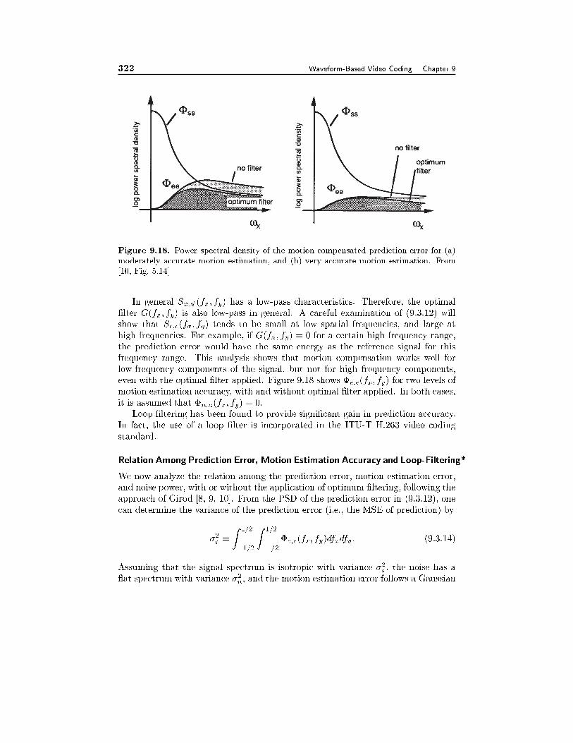
322 Waveform-Based Video Coding Chapter 9
Figure 9.18. Power spectral density of the motion compensated prediction error for (a)
moderately accurate motion estimation, and (b) very accurate motion estimation. From
[10, Fig. 5.14]
In general S ; (fx; fy) has a low-pass characteristics. Therefore, the optimal
�lter G(fx; fy) is also low-pass in general. A careful examination of (9.3.12) will
show that Se;e(fx; fy) tends to be small at low spatial frequencies, and large at
high frequencies. For example, if G(fx; fy) = 0 for a certain high frequency range,
the prediction error would have the same energy as the reference signal for this
frequency range. This analysis shows that motion compensation works well for
low-frequency components of the signal, but not for high frequency components,
even with the optimal �lter applied. Figure 9.18 shows �e;e(fx; fy) for two levels of
motion estimation accuracy, with and without optimal �lter applied. In both cases,
it is assumed that �n;n(fx; fy) = 0.
Loop �ltering has been found to provide signi�cant gain in prediction accuracy.
In fact, the use of a loop �lter is incorporated in the ITU-T H.263 video coding
standard.
Relation Among Prediction Error, Motion Estimation Accuracy and Loop-Filtering*
We now analyze the relation among the prediction error, motion estimation error,
and noise power, with or without the application of optimum �ltering, following the
approach of Girod [8, 9, 10]. From the PSD of the prediction error in (9.3.12), one
can determine the variance of the prediction error (i.e., the MSE of prediction) by
�2e =
Z 1=2
�1=2
Z 1=2
�1=2
�e;e(fx; fy)dfxdfy: (9.3.14)
Assuming that the signal spectrum is isotropic with variance �2s , the noise has a
at spectrum with variance �2n, and the motion estimation error follows a Gaussian
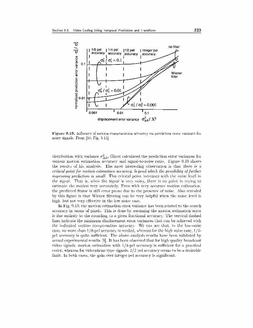
Section 9.3. Video Coding Using Temporal Prediction and Transform 323
Figure 9.19. In uence of motion compensation accuracy on prediction error variance for
noisy signals. From [10, Fig. 5.15]
distribution with variance �2�d, Girod calculated the prediction error variances for
various motion estimation accuracy and signal-to-noise ratio. Figure 9.19 shows
the results of his analysis. The most interesting observation is that there is a
critical point for motion estimation accuracy, beyond which the possibility of further
improving prediction is small. This critical point increases with the noise level in
the signal. That is, when the signal is very noisy, there is no point in trying to
estimate the motion very accurately. Even with very accurate motion estimation,
the predicted frame is still error prone due to the presence of noise. Also revealed
by this �gure is that Wiener �ltering can be very helpful when the noise level is
high, but not very e�ective in the low noise case.
In Fig. 9.19, the motion estimation error variance has been related to the search
accuracy in terms of pixels. This is done by assuming the motion estimation error
is due entirely to the rounding to a given fractional accuracy. The vertical dashed
lines indicate the minimum displacement error variances that can be achieved with
the indicated motion compensation accuracy. We can see that, in the low-noise
case, no more than 1/8-pel accuracy is needed, whereas for the high noise case, 1/2-
pel accuracy is quite suÆcient. The above analysis results have been validated by
actual experimental results [9]. It has been observed that for high quality broadcast
video signals, motion estimation with 1/4-pel accuracy is suÆcient for a practical
coder, whereas for videophone type signals, 1/2-pel accuracy seems to be a desirable
limit. In both cases, the gain over integer pel accuracy is signi�cant.
324 Waveform-Based Video Coding Chapter 9
9.4 Summary
Transform Coding (Sec. 9.1)
� Transform is a way to represent a group of samples (e.g. an image block) as
a linear combination of some basic patterns. The purpose of transform for
coding is to decorrelate original samples and compact the energy into a few
coeÆcients so that scalar quantization can be e�ectively applied. The optimal
transform under these criteria is the KLT.
� To achieve maximum gain from transform coding, one must appropriately
distribute bits among the coeÆcients. The optimal allocation (Eq. (9.1.43))
equalizes the distortion incurred by di�erent coeÆcients (Eq. (9.1.44)). The
�nal distortion depends on the geometric mean of the coeÆcient variances.
� The KLT depends on the second order statistics of the signal and thus is
image dependent and diÆcult to compute. DCT is a good approximation of
the KLT for most image signals and it can be computed using fast algorithms.
� DCT based coding method (Sec. 9.1.7) is an e�ective method for image coding
and has been employed in international standards for image and video coding.
� Optimization of quantization and binary encoding process is very important
in a transform coder. With similar quantization and binary encoding schemes,
DCT and wavelet transforms lead to similar coding eÆciency.
Predictive Coding (Sec. 9.2)
� The purpose of prediction is also to reduce the correlation between samples to
be coded, so that scalar quantization can be appplied e�ectively. The predictor
should be designed to minimize the prediction error. The LMMSE predictor
can be determined by solving the Yuler-Walker equation (Eq. (9.2.6)).
� To avoid the mismatch between the reference sample used for prediction in
the encoder and those in the decoder, closed-loop prediction is necessary, in
which the encoder must repeat the same operation of the decoder.
� Theoretically, predictive coding outperforms transform coding when the pre-
dictor order is the same as the transform length. However, the bit stream
resulting from predictive coding is very sensitive to transmission errors.
� For video coding, prediction can be performed in both spatial and temporal
domain. In the temporal direction, motion compensation is necessary to ac-
count for the e�ect of object motion. Only very low order predictors (usually
using only one previous frame) are used, to maintain a reasonable complexity,
and to reduce the e�ect of transmission error propagation.
Section 9.5. Problems 325
Block-Based Hybrid Video Coding (Sec. 9.3)
� The block-based hybrid coder (Sec. 9.3.1) combines motion compensated pre-
diction and transform coding e�ectively. Because of its relatively low com-
plexity and good coding eÆciency, it has been adopted in various international
standards for video coding (Chap. 13).
� Motion compensation accuracy can be improved by applying loop-�ltering
(Sec. 9.3.5), which suppresses the propagation of quantization errors in previ-
ous frames. The achievable motion compensation accuracy depends not only
on the motion estimation accuracy but also the loop-�lter used and the noise
level in the signal (Sec. 9.3.5).
� Within the framework of hybrid coders, the performance can be improved
by appropriately performing motion estimation and compensation (e.g. with
or without overlapping, �xed vs. variable block size) and selecting modes
of operations (intra vs. inter, prediction mode, etc.) The R-D optimized
approach chooses these coding options so that the distortion is minimized
under a given rate constraint. See Sec. 9.3.3.
� Rate control (Sec. 9.3.4) is an important issue in video coding, especially
for real-time applications, where excessive rates will lead to deterioration
(as opposed to improvement) in quality due to transmission delay and loss.
Rate control in hybrid coders are typically accomplished by adjusting frame
rates and quantization parameters, using either heuristic or R-D optimized
approaches.
� Coding mode selection and rate control can a�ect the performance of a coder
signi�cantly. Note that all the video coding standards using the hybrid cod-
ing framework only de�ne the bit stream syntax and consequently the decoder
operation. This gives the encoder exibility in optimizing its operation, in-
cluding motion estimation, coding mode selection and rate control. These are
typically the factors that di�erentiate di�erent video coding systems that all
conform to the same standard. Beyond coding eÆciency considerations, an-
other factor that can set apart di�erent systems is how does the encoder makes
the bit stream more resilient to transmission errors by judiciously selecting the
coding parameters within the standard framework, and how does the decoder
react to transmission errors. These issues are discussed in Chap. 14.
9.5 Problems
9.1 Prove the relations in Eqs. (9.1.11) to (9.1.16).
9.2 Con�rm that the 1-D DCT basis functions form an orthonormal basis.
9.3 Prove that a 2-D basis formed by the outer product of two orthonormal 1-D
bases is also orthonormal.
326 Waveform-Based Video Coding Chapter 9
9.4 Repeat Example 9.4 for the special case of �h = �v = �d = �:
9.5 Repeat Example 9.5 for the special case of �h = �v = �d = �: Compare the
KLT transform basis with the DCT.
9.6 Repeat Example 9.6 for the special case of �h = �v = �d = �:
9.7 Consider a predictive image coding system in which a pixel is predicted from
two pixels: one above and one to the left. Assume the image statistics is the
same as that considered in Example 9.4. Derive the optimal predictor and the
predictive coding gain. Compare the result with that in Example 9.6. Which
predictor is more eÆcient?
9.8 Write a C or Matlab code that examines the e�ect of approximating an image
with a partial set of DCT coeÆcients. Use 8� 8 DCT, reconstruct the image
with K < 64 coeÆcients, for K = 4; 8; 16; 32: How many coeÆcients are
necessary to provide a satisfactory reconstruction?
9.9 Write a C or Matlab code that examines the e�ect of quantization in the DCT
domain. Use 8� 8 DCT, and chose the quantization stepsizes to be multiples
of the normalization matrix given in Fig. 9.7. Try scale factors of 0.5, 1, 2, 4,
8, 16. What is the largest scale factor that still provides a satisfactory image?
9.10 Two simple transform coding methods are: i) only retain �rst K coeÆcients
(called zonal coding), and ii) only retain the coeÆcients that exceed a certain
threshold (called threshold coding). Discuss the pros and cons of these two
methods.
9.11 Consider the following three video coding methods: i) directly code a frame;
ii) code the di�erence between every two frames; iii) perform block-based mo-
tion estimation between every two frames and code the motion compensation
error image. Recall that the bit rate required to achieve a given distortion is
proportional to the variance of the signal to be coded. Take two adjacent video
frames from a sequence, calculate and compare the variances of i) a frame di-
rectly; ii) the direct di�erence between the two frames; and iii) the motion
compensation error image. Based on the result you get, can you determine
which of the three coding methods would be more eÆcient ?
9.12 Variance is only a crude indicator of the bit rate required. If we apply DCT
coding in each of the three methods in Prob. 9.11, a more accurate measure
of the bit rate is the number of DCT coeÆcients that are non-zero after quan-
tization with a chosen quantization parameter. Write a C or Matlab code to
perform this experiment.
9.13 Show that the optimal linear estimator solution for OBMC is as given in
Eq. (9.3.4).
Section 9.6. Bibliography 327
9.14 Show that the window function corresponding to the weighting coeÆcients
given in Fig. 9.16 is as given in Fig. 9.17. Draw it in the style of Fig. 9.15 and
comment on the similarity and di�erence between the two window functions.
9.15 Write a C- or matlab program that implements a basic form of the block-based
hybrid coder. For simplicity, only consider the intra-mode and the P-mode.
Except the �rst frame, which will be coded using the intra-mode entirely, each
MB in following frames will be coded using either the P-mode or intra-mode,
depending on whether the original MB or the motion compensation error has
the smaller variance. For motion estimation, you can choose to implement
either the EBMA or some fast algorithms. For the lossless coding part, you
can either use the Hu�man tables given a standard, e.g., [17], or estimating
the required bit rate by calculating the entropy of the symbols to be coded.
Apply the program to several test sequences with di�erent motion levels using
di�erent parameters: QP, frame rate, intra-fresh rate, etc. Evaluate the trade-
o� between rate and distortion and complexity (execution time). Play the
decompressed video to observe the coding artifacts with di�erent QP's.
9.6 Bibliography
[1] N. Ahmed, T. Natarajan, and K. R. Rao. Discrete Cosine Transform. IEEE
Trans. Computer, 23:90{93, 1974.
[2] B. Bellman. Dynamic Programming. Princeton University Press, 1957.
[3] M. C. Chen and A. N. Willson. Rate-distortion optimal motion estimation
algorithms for motion-compensated transform coding. IEEE Trans. Circuits Syst.
for Video Technology, 8(2):147{158, Apr. 1998.
[4] W-H. Chen et al. A fast computational algorithm for the discrete cosine trans-
form. IEEE Trans. Commun., COM-25:1004{1009, Sept. 1977.
[5] T. Chiang and Y.-Q. Zhang. A new rate control scheme using quadratic rate-
distortion model. IEEE Trans. Circuits Syst. for Video Technology, 7:246{250,
Sept. 1997.
[6] R. J. Clark. Transform Coding of Images. Academic Press, 1985.
[7] H. Everett. Generalized lagrange multiplier method for solving problems of
optimam allocation of resources. Operational Research, 11:399{417, 1963.
[8] B. Girod. The eÆciency of motion-compensating prediction for hybrid coding
of video sequences. IEEE J. Select. Areas Commun., SAC-5:1140{1154, 1987.
[9] B. Girod. Motion-compensating prediction with fractional-pel accuracy. IEEE
Trans. Commun., 41:604{612, 1993.
328 Waveform-Based Video Coding Chapter 9
[10] B. Girod. Motion compensation: visual aspects, accuracy, and fundamental
limits. In M. I. Sezan and R. L. Lagendijk, editors, Motion analysis and image
sequence processing, pages 126{152. Kluwer Academic Publishers, 1993.
[11] B. Girod. Rate-constrained motion estimation. In Proc. SPIE Conf. Visual
Commun. Image Processing, pages 1026{1034, Chicago, USA, Sept. 1994.
[12] R. G. Gonzalez and R. E. Woods. Digital Image Processing. Addison{Wesley,
2nd edition, 1992.
[13] C.-Y. Hsu, A. Ortega, and M. Khansari. Rate control for robust video transmis-
sion over burst-error wireless channels. IEEE J. Select. Areas Commun., 17(5):756{
773, May 1999.
[14] C.-Y. Hsu, A. Ortega, and A. R. Reibman. Joint selection and source and
channel rate for VBR video transmission under ATM policing constraints. IEEE
J. Select. Areas Commun., 15:1016{1028, Aug. 1997.
[15] ISO/IEC. IS 10918-1: Information technology { digital compression and coding
of continuous-tone still images: Requirements and guidelines, 1990. (JPEG).
[16] ISO/IEC. MPEG-2 Test Model 5 (TM5). Public document, ISO/IEC
JTC1/SC29/WG11/93-225b, Apr. 1993.
[17] ITU-T. Recommendation H.263: Video coding for low bit rate communication,
1998.
[18] A. K. Jain. Fundamentals of Digital Image Processing. Prentice Hall, 1989.
[19] N. S. Jayant and P. Noll. Digital Coding of Waveforms. Prentice-Hall, Inc.,
1984.
[20] F. Kossentini, Y.-W. Lee, M. J. T. Smith, and R. Ward. Predictive RD opti-
mized motion estimation for very low bit rate video coding. IEEE J. Select. Areas
Commun., 15(9):1752{1763, Dec. 1997.
[21] B. G. Lee. A new algorithm to compute discrete cosine transform. IEEE Trans.
Acoust., Speech, Signal Processing, ASSP-32:1243{1245, Dec. 1984.
[22] W. Li. Vector transform and image coding. IEEE Trans. Circuits Syst. for
Video Technology, 1(4):297{307, Dec. 1991.
[23] W. Li and Y.-Q. Zhang. Vector-based signal processing and quantization for
image and video compression. Proceedings of the IEEE, 83(2):317{333, Feb. 1995.
[24] J.-L. Lin and A. Ortega. Bit rate control using piecewise approximated rate-
distortion characteristics. IEEE Trans. Circuits Syst. for Video Technology, 8:446{
459, Aug. 1998.
Section 9.6. Bibliography 329
[25] S. Nogaki and M. Ohta. An overlapped block motion compensation for high
quality motion picture coding. In Proc. IEEE Int. Conf. Circuits and Systems,
pages 184{187, May 1992.
[26] M. T. Orchard and G. J. Sullivan. Overlapped block motion compensation:
An estimation-theoretic approach. IEEE Trans. Image Process., 3:693{699, 1994.
[27] A. Ortega. Variable bit rate video coding. In M. T. Sun and A. R. Reibman,
editors, Compressed Video over Networks. Marcel Dekker, Inc., 2001.
[28] A. Ortega and K. Ramchandran. Rate-distortion methods for image and video
compression. IEEE Signal Processing Magazine, 15:23{50, Nov. 1998.
[29] L. R. Rabiner and R. W. Shafer. Digital Processing of Speech Signals. Prentice
Hall, Englewood Cli�s, NJ, 1978.
[30] T. A. Ramstad. Considerations on quantization and dynamic bit allocation
in subband coders. In Proc. IEEE Int. Conf. Acoust., Speech, Signal Processing,
pages 841{844, Apr. 1986.
[31] G. M. Schuster and A. K. Katsaggelos. Rate-distortion based video compression.
Kluwer Academic Publishers, 1997.
[32] G. M. Schuster and A. K. Katsaggelos. A video compression scheme with
optimal bit allocation among segmentation, motion, and residual error. IEEE
Trans. Image Process., 6:1487{1501, Nov. 1997.
[33] A. Segall. Bit allocation and encoding for vector sources. IEEE Trans. Inform.
Theory, IT-22:162{169, Mar. 1976.
[34] G. J. Sullivan and R. L. Baker. Rate-distortion optimized motion compensation
for video compression using �xed vs. variable size blocks. In Global Telecomm.
Conf. (GLOBECOM'91), pages 85{90, Dec. 1991.
[35] G. J. Sullivan and T. Wiegand. Rate-distortion optimization for video com-
pression. IEEE Signal Processing Magazine, 15:74{90, Nov. 1998.
[36] A. Vetro, H. Sun, and Y. Wang. MPEG-4 rate control for multiple video
objects. IEEE Trans. Circuits Syst. for Video Technology, 9:186{199, Feb. 1999.
[37] T. Wiegand, M. Lightstone, D. Mukherjee, T. Campell, and S. K. Mitra.
Rate-distortion optimized mode selection for very low bit rate video coding and
the emerging H.263 standard. IEEE Trans. Circuits Syst. for Video Technology,
6(2):182{190, Apr. 1996.
Chapter 10
CONTENT DEPENDENT
VIDEO CODING
In Section (8.1), we gave an overview on di�erent video coding systems. One way
of distinguishing di�erent coding systems is to compare their source models. Video
coding based on source models that do not adapt to the shape of moving objects in
a video sequence were described in Chapter 9. In this chapter, we focus on video
coding algorithms that consider the shape of the objects in the video sequence. In
order to eÆciently transmit arbitrarily shaped video objects, we have to code the
object shape as well as the texture for these arbitrarily-shaped objects. In Section
10.1 we describe several methods for coding the 2D shape of an object. Section
10.2 presents algorithms to eÆciently code the texture of these segments. Two
algorithms coding shape and texture jointly are brie y described in Section 10.3.
In the following sections 10.4 and 10.5, we describe how these techniques can be
used in region-based and object-based coding, respectively. Object-based coding
may be based on 2D and 3D object models. Using 3D object models, object-based
coding can be extended to knowledge-based and semantic coding as described in
Sections 10.6 and 10.7. In Section 10.8 we present a concept that allows to integrate
conventional block-based hybrid coders with object-based coding, knowledge-based
coding and semantic coding.
10.1 2D Shape Coding
The 2D shape of an object, say the k-th object, is de�ned by means of an alpha-map
Mk:
Mk = fmk(x; y)j0 � x � X; 0 � y � Y g; 0 � mk � 255: (10.1.1)
The shape Mk de�nes for each pel x = (x; y) whether it belongs to the object
(mk(x) > 0) or not (mk(x) = 0). For an opaque object, the corresponding alpha-
values are 255, for transparent objects they range from 0 to 255. Usually, the
alpha-map has the same spatial and temporal resolution as the luminance signal of
the video sequence. In video editing applications, the alpha-map is used to describe
object shape and object transparency. Let us assume that we have a background
330
Section 10.1. 2D Shape Coding 331
image b(x), the object represented by image o(x) and the alpha-map mo(x).
Overlaying the object on the background is done according to
(x) =
�1�
mo(x)
255
�� b(x) +
mo(x)
255� o(x) (10.1.2)
The amplitude of the alpha-map determines how visible the object becomes. In
this chapter, we will only deal with binary object shape, i.e. mk(x) 2 f0; 255gThere are two classes of binary shape coders. A bitmap-based coder (Section
10.1.1) encodes for each pel whether it belongs to the object or not. A contour -based
coder (Section 10.1.2) encodes the outline of the object. In order to retrieve the
bitmap of the object shape, the contour is �lled with the object label. In the case
that there is also texture transmitted with the shape information, an implicit shape
coder can be used where the shape information can be derived from the texture (see
Section 10.3). Similar to texture coding, binary shapes can be coded in a lossless
or lossy fashion. Therefore, it is important to de�ne a measure for the quality of
lossily encoded shapes (Section 10.1.3).
10.1.1 Bitmap Coding
A bitmap-based shape coder speci�es a binary alpha-map. In its simplest form, we
scan the alpha-map and transmit for each pel a 0 or 1 depending on whether it
belongs to the object. Such an algorithm is ineÆcient because it does not consider
statistical dependencies between neighboring pels. In this section, we describe three
ways of improving coding eÆciency: One class scans the bitmap in scan line order
and speci�es the run-lengths of black and white pels, a second class of algorithms
codes each pel of the bitmap based on the colors of th neighboring pels, and the third
class de�nes the shape as a tree of basic shapes arranged such that they completely
�ll the object shape.
Scan Line Coding
In this method, we scan the image line by line and transmit the run of black and
white pels using a variable length coder thus exploiting one-dimensional correlation
between pels. This method is used in the FAX standard G3 [36]. Next we discuss
an extension of this coder that also considers the correlation between neighboring
scan lines.
The modi�ed READ code (Relative Element Address Designate) as used in the
FAX standards G4 [20] and JBIG [21] codes one scan line with respect to the
previous scan line thus exploiting 2D correlation. The algorithm scans each line of
the document and encodes the location of changing pels where the scan line changes
its color (Fig. 10.1). In this line-by-line scheme the position of each changing pel
on the current line is coded with respect to either the position of a corresponding
changing pel in the reference line, which lies immediately above the present line, or
with respect to the preceding changing pel in the current line [36]. Figure 10.1 is
used to explain one implementation of an modi�ed READ coder. We assume that
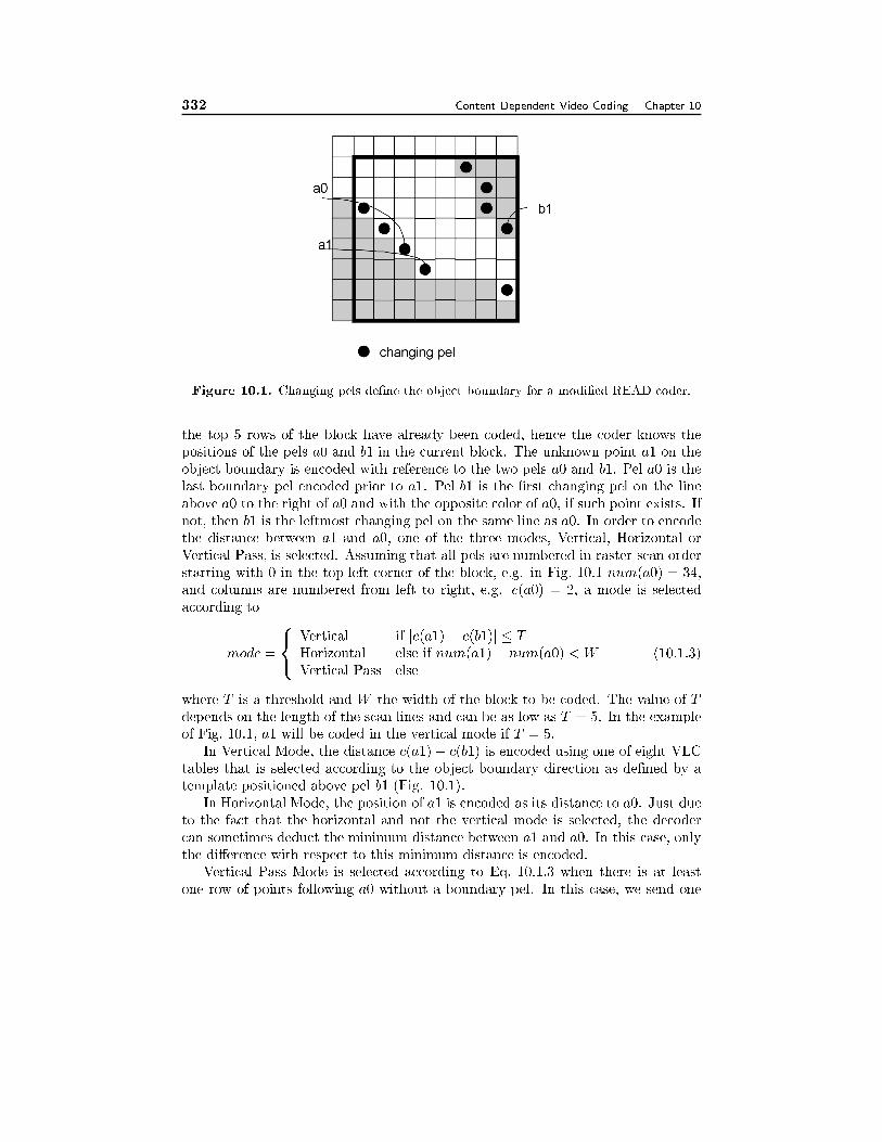
332 Content Dependent Video Coding Chapter 10
Figure 10.1. Changing pels de�ne the object boundary for a modi�ed READ coder.
the top 5 rows of the block have already been coded, hence the coder knows the
positions of the pels a0 and b1 in the current block. The unknown point a1 on the
object boundary is encoded with reference to the two pels a0 and b1. Pel a0 is the
last boundary pel encoded prior to a1. Pel b1 is the �rst changing pel on the line
above a0 to the right of a0 and with the opposite color of a0, if such point exists. If
not, then b1 is the leftmost changing pel on the same line as a0. In order to encode
the distance between a1 and a0, one of the three modes, Vertical, Horizontal or
Vertical Pass, is selected. Assuming that all pels are numbered in raster-scan order
starting with 0 in the top-left corner of the block, e.g. in Fig. 10.1 num(a0) = 34,
and columns are numbered from left to right, e.g. c(a0) = 2, a mode is selected
according to
mode =
8<:
Vertical if jc(a1)� c(b1)j � T
Horizontal else if num(a1)� num(a0) < W
Vertical Pass else
(10.1.3)
where T is a threshold and W the width of the block to be coded. The value of T
depends on the length of the scan lines and can be as low as T = 5. In the example
of Fig. 10.1, a1 will be coded in the vertical mode if T = 5:
In Vertical Mode, the distance c(a1)� c(b1) is encoded using one of eight VLC
tables that is selected according to the object boundary direction as de�ned by a
template positioned above pel b1 (Fig. 10.1).
In Horizontal Mode, the position of a1 is encoded as its distance to a0. Just due
to the fact that the horizontal and not the vertical mode is selected, the decoder
can sometimes deduct the minimum distance between a1 and a0. In this case, only
the di�erence with respect to this minimum distance is encoded.
Vertical Pass Mode is selected according to Eq. 10.1.3 when there is at least
one row of points following a0 without a boundary pel. In this case, we send one
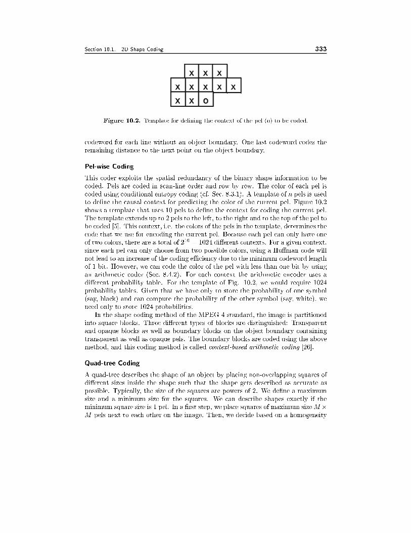
Section 10.1. 2D Shape Coding 333
Figure 10.2. Template for de�ning the context of the pel (o) to be coded.
codeword for each line without an object boundary. One last codeword codes the
remaining distance to the next point on the object boundary.
Pel-wise Coding
This coder exploits the spatial redundancy of the binary shape information to be
coded. Pels are coded in scan-line order and row by row. The color of each pel is
coded using conditional entropy coding (cf. Sec. 8.3.1). A template of n pels is used
to de�ne the causal context for predicting the color of the current pel. Figure 10.2
shows a template that uses 10 pels to de�ne the context for coding the current pel.
The template extends up to 2 pels to the left, to the right and to the top of the pel to
be coded [5]. This context, i.e. the colors of the pels in the template, determines the
code that we use for encoding the current pel. Because each pel can only have one
of two colors, there are a total of 210 = 1024 di�erent contexts. For a given context,
since each pel can only choose from two possible colors, using a Hu�man code will
not lead to an increase of the coding eÆciency due to the minimum codeword length
of 1 bit. However, we can code the color of the pel with less than one bit by using
an arithmetic coder (Sec. 8.4.2). For each context the arithmetic encoder uses a
di�erent probability table. For the template of Fig. 10.2, we would require 1024
probability tables. Given that we have only to store the probability of one symbol
(say, black) and can compute the probability of the other symbol (say, white), we
need only to store 1024 probabilities.
In the shape coding method of the MPEG-4 standard, the image is partitioned
into square blocks. Three di�erent types of blocks are distinguished: Transparent
and opaque blocks as well as boundary blocks on the object boundary containing
transparent as well as opaque pels. The boundary blocks are coded using the above
method, and this coding method is called context-based arithmetic coding [26].
Quad-tree Coding
A quad-tree describes the shape of an object by placing non-overlapping squares of
di�erent sizes inside the shape such that the shape gets described as accurate as
possible. Typically, the size of the squares are powers of 2. We de�ne a maximum
size and a minimum size for the squares. We can describe shapes exactly if the
minimum square size is 1 pel. In a �rst step, we place squares of maximum sizeM�M pels next to each other on the image. Then, we decide based on a homogeneity
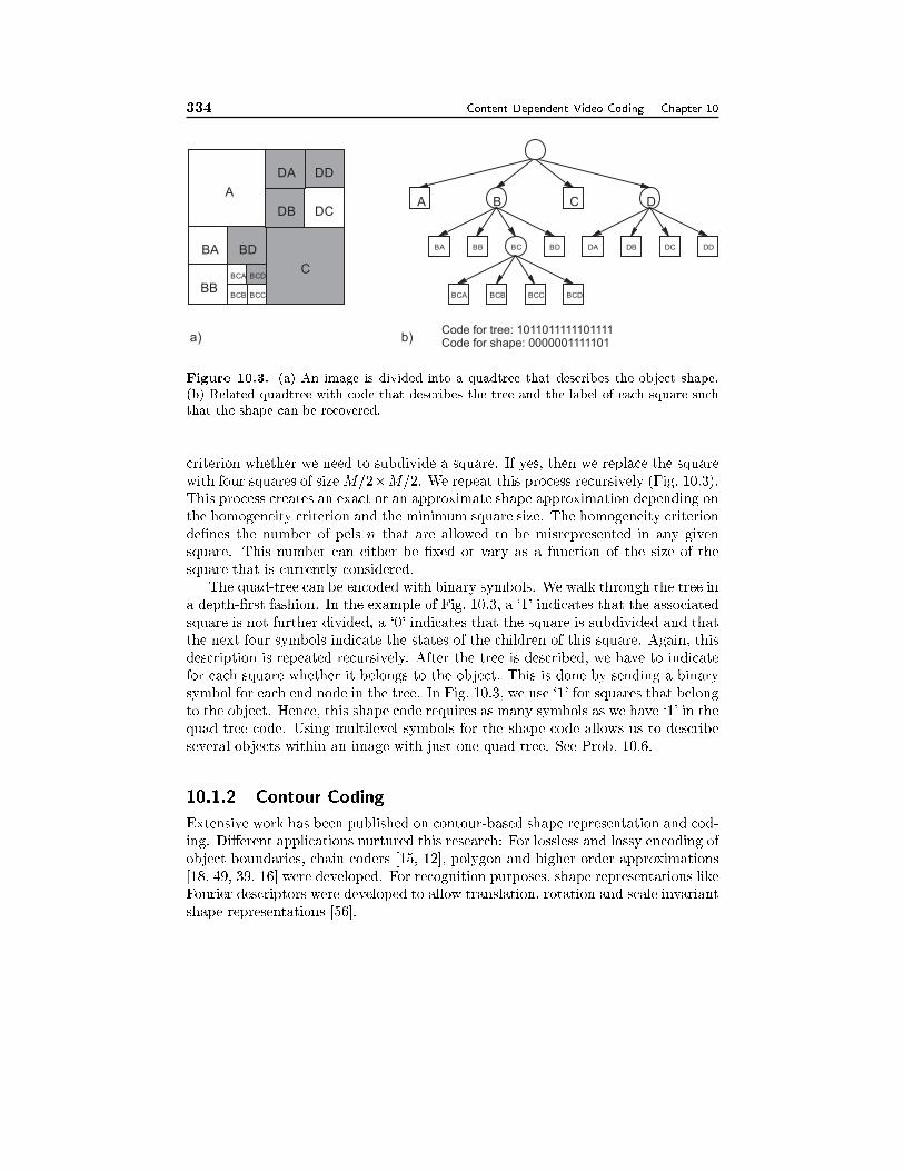
334 Content Dependent Video Coding Chapter 10
A
BB
BA BD
DA
DB DC
DD
BCA
BCB BCC
BCD
A
A D
BBBA BD DA DB DC DD
BCA BCB BCC BCD
C
B C
BC
a) b)Code for tree: 1011011111101111Code for shape: 0000001111101
Figure 10.3. (a) An image is divided into a quadtree that describes the object shape.
(b) Related quadtree with code that describes the tree and the label of each square such
that the shape can be recovered.
criterion whether we need to subdivide a square. If yes, then we replace the square
with four squares of sizeM=2�M=2. We repeat this process recursively (Fig. 10.3).
This process creates an exact or an approximate shape approximation depending on
the homogeneity criterion and the minimum square size. The homogeneity criterion
de�nes the number of pels n that are allowed to be misrepresented in any given
square. This number can either be �xed or vary as a function of the size of the
square that is currently considered.
The quad-tree can be encoded with binary symbols. We walk through the tree in
a depth-�rst fashion. In the example of Fig. 10.3, a `1' indicates that the associated
square is not further divided, a `0' indicates that the square is subdivided and that
the next four symbols indicate the states of the children of this square. Again, this
description is repeated recursively. After the tree is described, we have to indicate
for each square whether it belongs to the object. This is done by sending a binary
symbol for each end node in the tree. In Fig. 10.3, we use `1' for squares that belong
to the object. Hence, this shape code requires as many symbols as we have `1' in the
quad-tree code. Using multilevel symbols for the shape code allows us to describe
several objects within an image with just one quad-tree. See Prob. 10.6.
10.1.2 Contour Coding
Extensive work has been published on contour-based shape representation and cod-
ing. Di�erent applications nurtured this research: For lossless and lossy encoding of
object boundaries, chain coders [15, 12], polygon and higher order approximations
[18, 49, 39, 16] were developed. For recognition purposes, shape representations like
Fourier descriptors were developed to allow translation, rotation and scale invariant
shape representations [56].
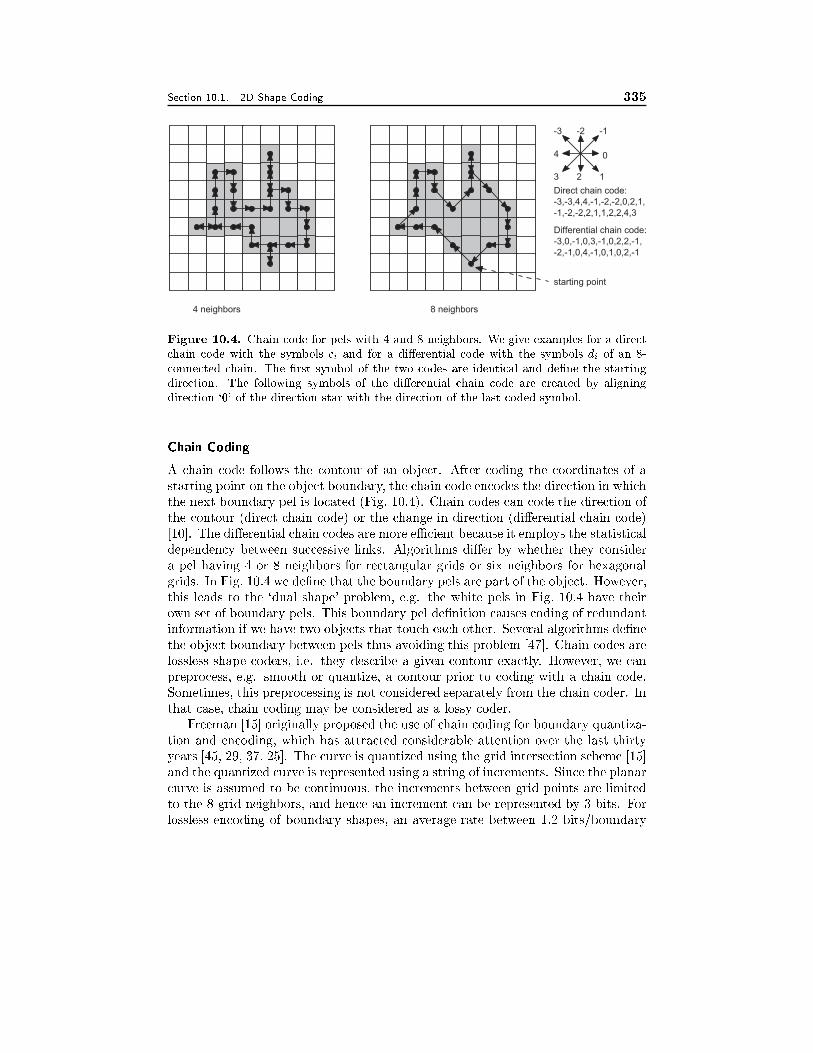
Section 10.1. 2D Shape Coding 335
0
-1-2-3
4
3 2 1
Direct chain code:
-3,-3,4,4,-1,-2,-2,0,2,1,
-1,-2,-2,2,1,1,2,2,4,3
4 neighbors 8 neighbors
starting point
Differential chain code:
-3,0,-1,0,3,-1,0,2,2,-1,
-2,-1,0,4,-1,0,1,0,2,-1
Figure 10.4. Chain code for pels with 4 and 8 neighbors. We give examples for a direct
chain code with the symbols ci and for a di�erential code with the symbols di of an 8-
connected chain. The �rst symbol of the two codes are identical and de�ne the starting
direction. The following symbols of the di�erential chain code are created by aligning
direction `0' of the direction star with the direction of the last coded symbol.
Chain Coding
A chain code follows the contour of an object. After coding the coordinates of a
starting point on the object boundary, the chain code encodes the direction in which
the next boundary pel is located (Fig. 10.4). Chain codes can code the direction of
the contour (direct chain code) or the change in direction (di�erential chain code)
[10]. The di�erential chain codes are more eÆcient because it employs the statistical
dependency between successive links. Algorithms di�er by whether they consider
a pel having 4 or 8 neighbors for rectangular grids or six neighbors for hexagonal
grids. In Fig. 10.4 we de�ne that the boundary pels are part of the object. However,
this leads to the `dual shape' problem, e.g. the white pels in Fig. 10.4 have their
own set of boundary pels. This boundary pel de�nition causes coding of redundant
information if we have two objects that touch each other. Several algorithms de�ne
the object boundary between pels thus avoiding this problem [47]. Chain codes are
lossless shape coders, i.e. they describe a given contour exactly. However, we can
preprocess, e.g. smooth or quantize, a contour prior to coding with a chain code.
Sometimes, this preprocessing is not considered separately from the chain coder. In
that case, chain coding may be considered as a lossy coder.
Freeman [15] originally proposed the use of chain coding for boundary quantiza-
tion and encoding, which has attracted considerable attention over the last thirty
years [45, 29, 37, 25]. The curve is quantized using the grid intersection scheme [15]
and the quantized curve is represented using a string of increments. Since the planar
curve is assumed to be continuous, the increments between grid points are limited
to the 8 grid neighbors, and hence an increment can be represented by 3 bits. For
lossless encoding of boundary shapes, an average rate between 1.2 bits/boundary
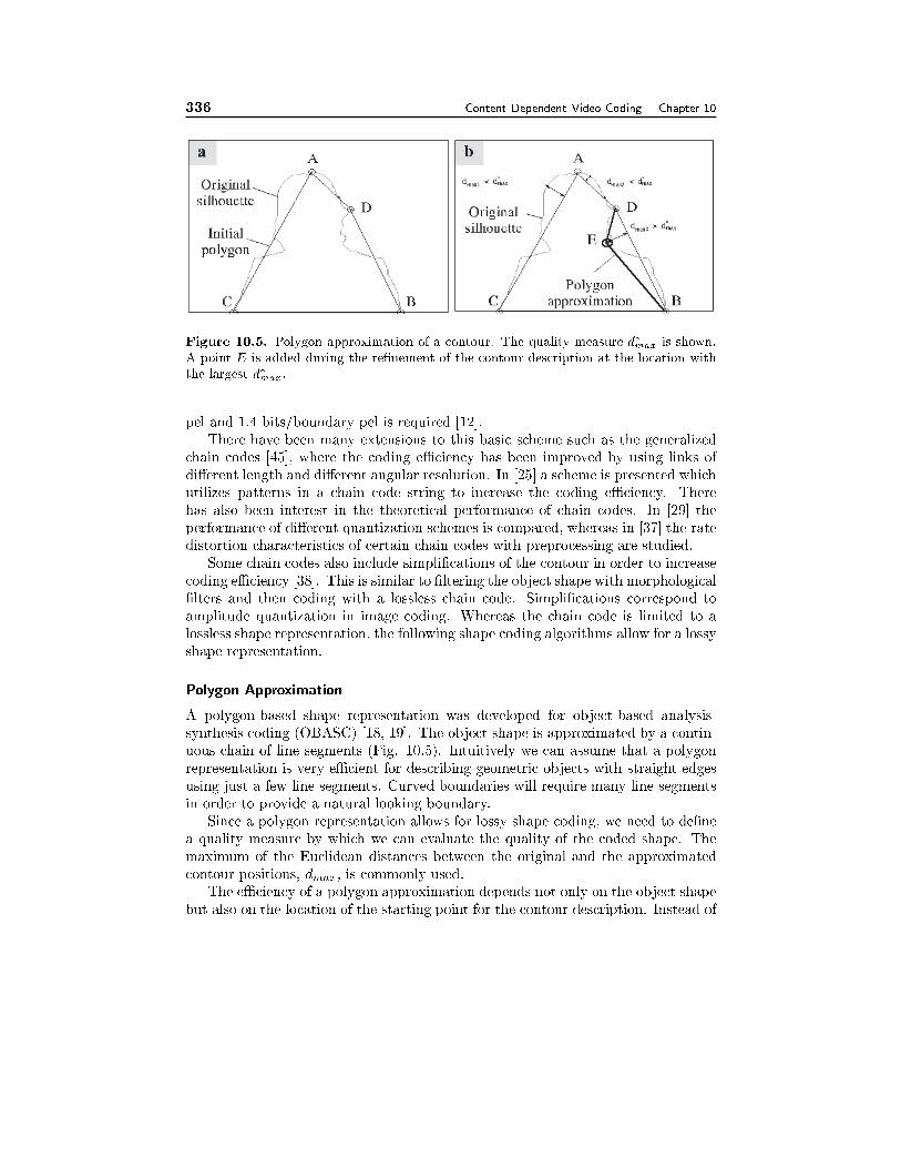
336 Content Dependent Video Coding Chapter 10
Figure 10.5. Polygon approximation of a contour. The quality measure d�
max is shown.
A point E is added during the re�nement of the contour description at the location with
the largest d�max.
pel and 1.4 bits/boundary pel is required [12].
There have been many extensions to this basic scheme such as the generalized
chain codes [45], where the coding eÆciency has been improved by using links of
di�erent length and di�erent angular resolution. In [25] a scheme is presented which
utilizes patterns in a chain code string to increase the coding eÆciency. There
has also been interest in the theoretical performance of chain codes. In [29] the
performance of di�erent quantization schemes is compared, whereas in [37] the rate
distortion characteristics of certain chain codes with preprocessing are studied.
Some chain codes also include simpli�cations of the contour in order to increase
coding eÆciency [38]. This is similar to �ltering the object shape with morphological
�lters and then coding with a lossless chain code. Simpli�cations correspond to
amplitude quantization in image coding. Whereas the chain code is limited to a
lossless shape representation, the following shape coding algorithms allow for a lossy
shape representation.
Polygon Approximation
A polygon-based shape representation was developed for object-based analysis-
synthesis coding (OBASC) [18, 19]. The object shape is approximated by a contin-
uous chain of line segments (Fig. 10.5). Intuitively we can assume that a polygon
representation is very eÆcient for describing geometric objects with straight edges
using just a few line segments. Curved boundaries will require many line segments
in order to provide a natural looking boundary.
Since a polygon representation allows for lossy shape coding, we need to de�ne
a quality measure by which we can evaluate the quality of the coded shape. The
maximum of the Euclidean distances between the original and the approximated
contour positions, dmax, is commonly used.
The eÆciency of a polygon approximation depends not only on the object shape
but also on the location of the starting point for the contour description. Instead of
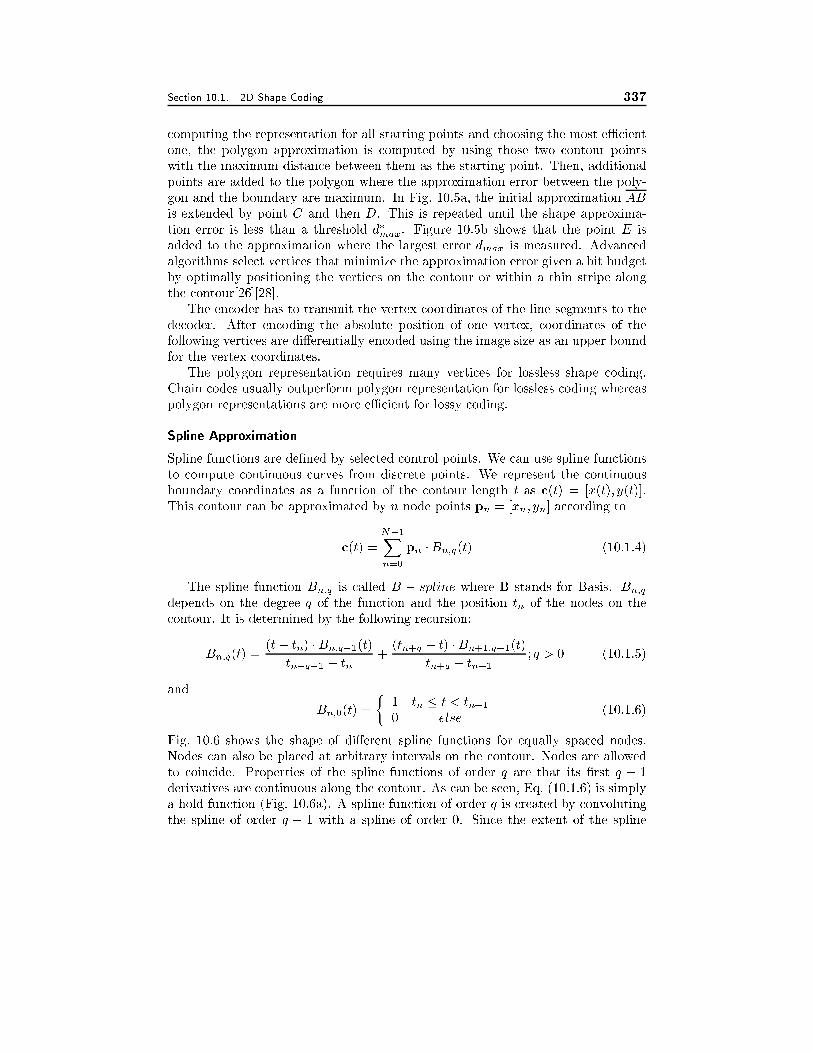
Section 10.1. 2D Shape Coding 337
computing the representation for all starting points and choosing the most eÆcient
one, the polygon approximation is computed by using those two contour points
with the maximum distance between them as the starting point. Then, additional
points are added to the polygon where the approximation error between the poly-
gon and the boundary are maximum. In Fig. 10.5a, the initial approximation AB
is extended by point C and then D. This is repeated until the shape approxima-
tion error is less than a threshold d�max. Figure 10.5b shows that the point E is
added to the approximation where the largest error dmax is measured. Advanced
algorithms select vertices that minimize the approximation error given a bit budget
by optimally positioning the vertices on the contour or within a thin stripe along
the contour[26][28].
The encoder has to transmit the vertex coordinates of the line segments to the
decoder. After encoding the absolute position of one vertex, coordinates of the
following vertices are di�erentially encoded using the image size as an upper bound
for the vertex coordinates.
The polygon representation requires many vertices for lossless shape coding.
Chain codes usually outperform polygon representation for lossless coding whereas
polygon representations are more eÆcient for lossy coding.
Spline Approximation
Spline functions are de�ned by selected control points. We can use spline functions
to compute continuous curves from discrete points. We represent the continuous
boundary coordinates as a function of the contour length t as c(t) = [x(t); y(t)].
This contour can be approximated by n node points pn = [xn; yn] according to
c(t) =
N�1Xn=0
pn �Bn;q(t) (10.1.4)
The spline function Bn;q is called B � spline where B stands for Basis. Bn;q
depends on the degree q of the function and the position tn of the nodes on the
contour. It is determined by the following recursion:
Bn;q(t) =(t� tn) �Bn;q�1(t)
tn+q�1 � tn+
(tn+q � t) �Bn+1;q�1(t)
tn+q � tn�1; q > 0 (10.1.5)
and
Bn;0(t) =
�1 tn � t < tn+10 else
(10.1.6)
Fig. 10.6 shows the shape of di�erent spline functions for equally spaced nodes.
Nodes can also be placed at arbitrary intervals on the contour. Nodes are allowed
to coincide. Properties of the spline functions of order q are that its �rst q � 1
derivatives are continuous along the contour. As can be seen, Eq. (10.1.6) is simply
a hold function (Fig. 10.6a). A spline function of order q is created by convoluting
the spline of order q � 1 with a spline of order 0. Since the extent of the spline
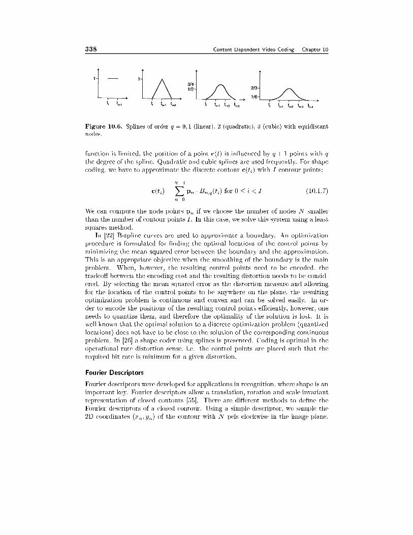
338 Content Dependent Video Coding Chapter 10
Figure 10.6. Splines of order q = 0; 1 (linear), 2 (quadratic), 3 (cubic) with equidistant
nodes.
function is limited, the position of a point c(t) is in uenced by q + 1 points with q
the degree of the spline. Quadratic and cubic splines are used frequently. For shape
coding, we have to approximate the discrete contour c(ti) with I contour points:
c(ti) =
N�1Xn=0
pn � Bn;q(ti) for 0 � i < I (10.1.7)
We can compute the node points pn if we choose the number of nodes N smaller
than the number of contour points I . In this case, we solve this system using a least
squares method.
In [22] B-spline curves are used to approximate a boundary. An optimization
procedure is formulated for �nding the optimal locations of the control points by
minimizing the mean squared error between the boundary and the approximation.
This is an appropriate objective when the smoothing of the boundary is the main
problem. When, however, the resulting control points need to be encoded, the
tradeo� between the encoding cost and the resulting distortion needs to be consid-
ered. By selecting the mean squared error as the distortion measure and allowing
for the location of the control points to be anywhere on the plane, the resulting
optimization problem is continuous and convex and can be solved easily. In or-
der to encode the positions of the resulting control points eÆciently, however, one
needs to quantize them, and therefore the optimality of the solution is lost. It is
well known that the optimal solution to a discrete optimization problem (quantized
locations) does not have to be close to the solution of the corresponding continuous
problem. In [26] a shape coder using splines is presented. Coding is optimal in the
operational rate distortion sense, i.e. the control points are placed such that the
required bit rate is minimum for a given distortion.
Fourier Descriptors
Fourier descriptors were developed for applications in recognition, where shape is an
important key. Fourier descriptors allow a translation, rotation and scale invariant
representation of closed contours [55]. There are di�erent methods to de�ne the
Fourier descriptors of a closed contour. Using a simple descriptor, we sample the
2D coordinates (xn; yn) of the contour with N pels clockwise in the image-plane.
Section 10.1. 2D Shape Coding 339
We represent the coordinates as a complex number zn = xn + j � yn and compute
the Fourier series as
Z(m) =
N�1Xn=0
z(n) � e�j2�nm
N (10.1.8)
Smooth contours will have their energy concentrated in the lower frequencies of the
Fourier series. Setting higher frequency coeÆcients to 0 smoothes a contour.
It can be shown from Eq. (10.1.8) that a translation of the contour will only
in uence coeÆcient Z(0), the DC value. Scaling of the contour will multiply all
coeÆcients with the scale factor. Rotation of the contour will shift the phase of the
Fourier coeÆcients but it will not e�ect their amplitude.
Another way of computing Fourier descriptors is to transform the list of 2D
coordinates (xn; yn) into an ordered list (n; (yn+1�yn)=(xn+1�xn)) with (x0; y0) =(xN ; yN) and 0 � n � N being the contour points. The term (yn+1�yn)=(xn+1�xn)describes the change of direction of the contour. The Fourier series of this descriptor
compacts more energy into the lower coeÆcients. This is partially due to the fact
that the DC value describes a circle, which has constant change of direction, instead
of a straight line as in Eq. (10.1.8).
In order to preserve the main characteristics of a shape, only the large Fourier
coeÆcients have to be maintained. Fourier descriptors are not very eÆcient in
reconstructing polygon-like shapes with only a few coeÆcients. This is one of the
reasons that they never became very competitive in terms of coding eÆciency.
10.1.3 Evaluation Criteria for Shape Coding EÆciency
Lossy shape coding can create two di�erent types of distortions:
� The contour of an object might get changed. Sharp corners get smoothed,
parts of the contour get displaced by a small number of pels.
� The topology of an object gets changed, i.e. the object might get additional
holes, holes are closed or parts of the object get disconnected from the original
shape.
There are two commonly used quality measures for objectively assessing the
quality of coded shape parameters. The peak deviation d�max is the maximum of the
Euclidean distances between each coded contour point and the closest point on the
original contour. This measure allows for an easy interpretation of the shape quality
due to changes of the object contours. However, if lossy shape coding results in
changing the topology of an object, the peak deviation d�max is not a useful measure.
A second measure dn depends of the number of pels that belong to the object and its
coded representation. The metric dn is the number of erroneously represented pels
of the coded shape divided by the total number of pels belonging to the original
shape. Since di�erent objects can have very di�erent ratios of contour pels to
interior pels, a given value for dn only allows to compare di�erent approximations
of the same object. The quality measure dn by itself does not provide suÆcient
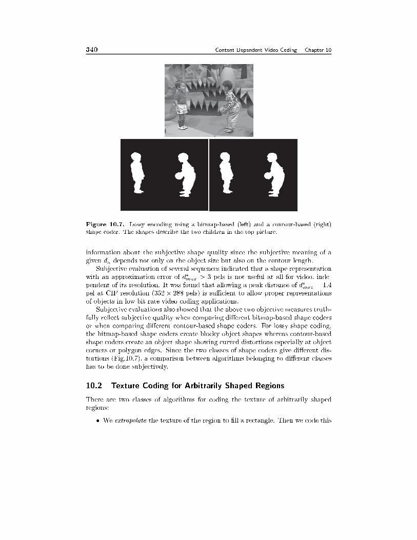
340 Content Dependent Video Coding Chapter 10
Figure 10.7. Lossy encoding using a bitmap-based (left) and a contour-based (right)
shape coder. The shapes describe the two children in the top picture.
information about the subjective shape quality since the subjective meaning of a
given dn depends not only on the object size but also on the contour length.
Subjective evaluation of several sequences indicated that a shape representation
with an approximation error of d�max > 3 pels is not useful at all for video, inde-
pendent of its resolution. It was found that allowing a peak distance of d�max = 1:4
pel at CIF resolution (352� 288 pels) is suÆcient to allow proper representations
of objects in low bit rate video coding applications.
Subjective evaluations also showed that the above two objective measures truth-
fully re ect subjective quality when comparing di�erent bitmap-based shape coders
or when comparing di�erent contour-based shape coders. For lossy shape coding,
the bitmap-based shape coders create blocky object shapes whereas contour-based
shape coders create an object shape showing curved distortions especially at object
corners or polygon edges. Since the two classes of shape coders give di�erent dis-
tortions (Fig.10.7), a comparison between algorithms belonging to di�erent classes
has to be done subjectively.
10.2 Texture Coding for Arbitrarily Shaped Regions
There are two classes of algorithms for coding the texture of arbitrarily shaped
regions:
� We extrapolate the texture of the region to �ll a rectangle. Then we code this
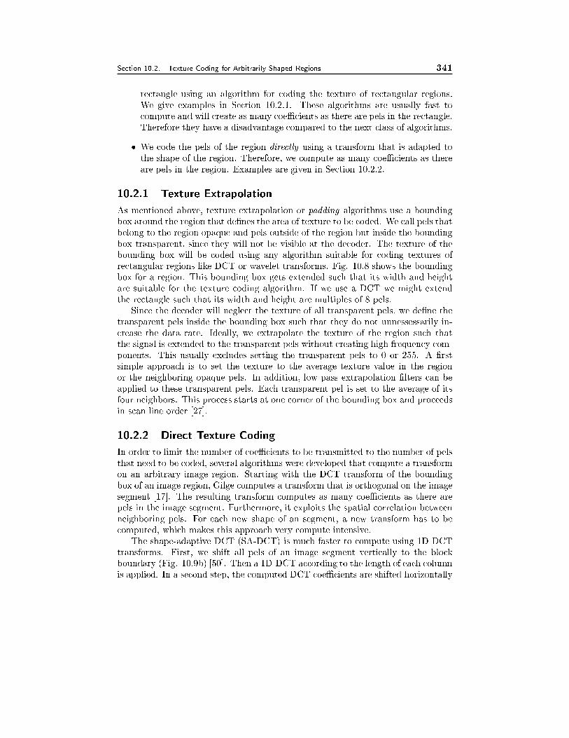
Section 10.2. Texture Coding for Arbitrarily Shaped Regions 341
rectangle using an algorithm for coding the texture of rectangular regions.
We give examples in Section 10.2.1. These algorithms are usually fast to
compute and will create as many coeÆcients as there are pels in the rectangle.
Therefore they have a disadvantage compared to the next class of algorithms.
� We code the pels of the region directly using a transform that is adapted to
the shape of the region. Therefore, we compute as many coeÆcients as there
are pels in the region. Examples are given in Section 10.2.2.
10.2.1 Texture Extrapolation
As mentioned above, texture extrapolation or padding algorithms use a bounding
box around the region that de�nes the area of texture to be coded. We call pels that
belong to the region opaque and pels outside of the region but inside the bounding
box transparent, since they will not be visible at the decoder. The texture of the
bounding box will be coded using any algorithm suitable for coding textures of
rectangular regions like DCT or wavelet transforms. Fig. 10.8 shows the bounding
box for a region. This bounding box gets extended such that its width and height
are suitable for the texture coding algorithm. If we use a DCT we might extend
the rectangle such that its width and height are multiples of 8 pels.
Since the decoder will neglect the texture of all transparent pels, we de�ne the
transparent pels inside the bounding box such that they do not unnessessarily in-
crease the data rate. Ideally, we extrapolate the texture of the region such that
the signal is extended to the transparent pels without creating high frequency com-
ponents. This usually excludes setting the transparent pels to 0 or 255. A �rst
simple approach is to set the texture to the average texture value in the region
or the neighboring opaque pels. In addition, low pass extrapolation �lters can be
applied to these transparent pels. Each transparent pel is set to the average of its
four neighbors. This process starts at one corner of the bounding box and proceeds
in scan line order [27].
10.2.2 Direct Texture Coding
In order to limit the number of coeÆcients to be transmitted to the number of pels
that need to be coded, several algorithms were developed that compute a transform
on an arbitrary image region. Starting with the DCT transform of the bounding
box of an image region, Gilge computes a transform that is orthogonal on the image
segment [17]. The resulting transform computes as many coeÆcients as there are
pels in the image segment. Furthermore, it exploits the spatial correlation between
neighboring pels. For each new shape of an segment, a new transform has to be
computed, which makes this approach very compute intensive.
The shape-adaptive DCT (SA-DCT) is much faster to compute using 1D DCT
transforms. First, we shift all pels of an image segment vertically to the block
boundary (Fig. 10.9b) [50]. Then a 1D-DCT according to the length of each column
is applied. In a second step, the computed DCT coeÆcients are shifted horizontally
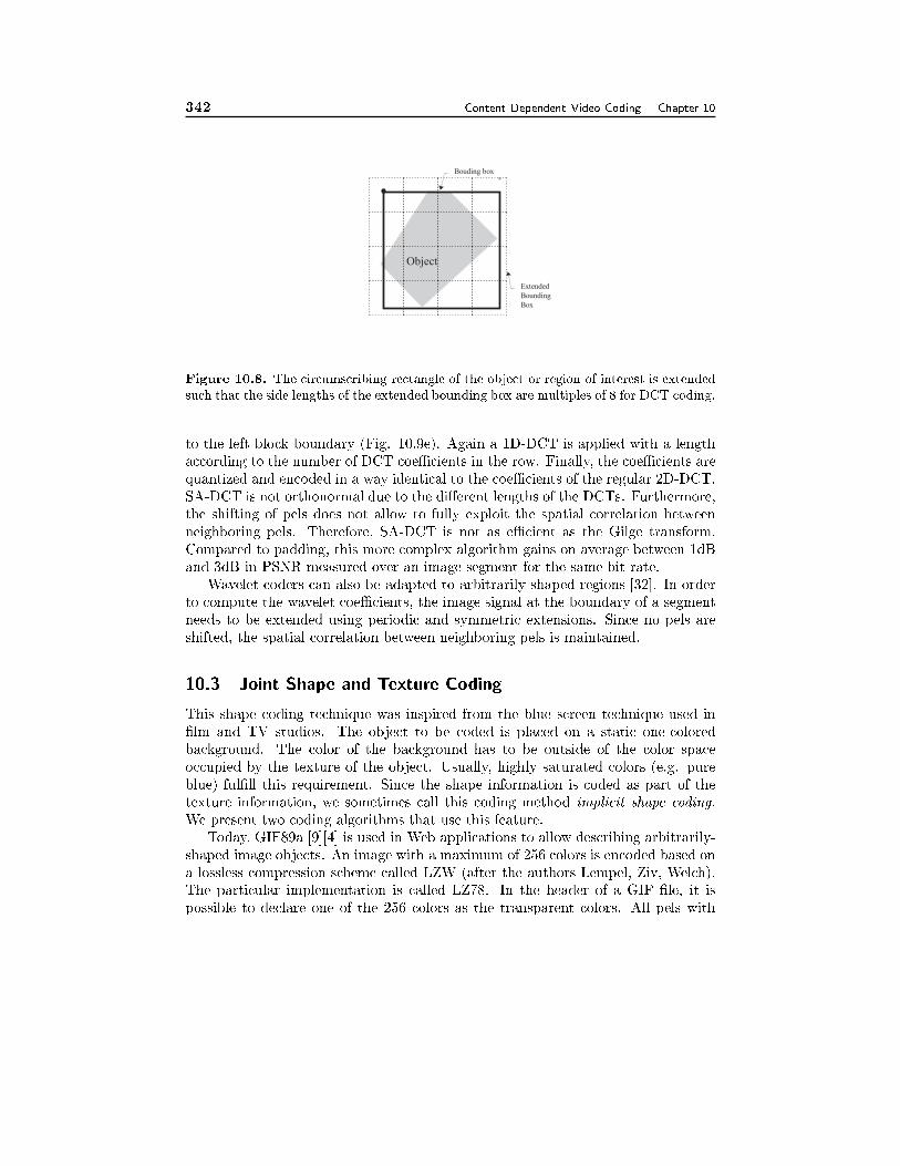
342 Content Dependent Video Coding Chapter 10
Bouding box
Extended
Bounding
Box
Object
Figure 10.8. The circumscribing rectangle of the object or region of interest is extended
such that the side lengths of the extended bounding box are multiples of 8 for DCT coding.
to the left block boundary (Fig. 10.9e). Again a 1D-DCT is applied with a length
according to the number of DCT coeÆcients in the row. Finally, the coeÆcients are
quantized and encoded in a way identical to the coeÆcients of the regular 2D-DCT.
SA-DCT is not orthonormal due to the di�erent lengths of the DCTs. Furthermore,
the shifting of pels does not allow to fully exploit the spatial correlation between
neighboring pels. Therefore, SA-DCT is not as eÆcient as the Gilge transform.
Compared to padding, this more complex algorithm gains on average between 1dB
and 3dB in PSNR measured over an image segment for the same bit rate.
Wavelet coders can also be adapted to arbitrarily shaped regions [32]. In order
to compute the wavelet coeÆcients, the image signal at the boundary of a segment
needs to be extended using periodic and symmetric extensions. Since no pels are
shifted, the spatial correlation between neighboring pels is maintained.
10.3 Joint Shape and Texture Coding
This shape coding technique was inspired from the blue screen technique used in
�lm and TV studios. The object to be coded is placed on a static one-colored
background. The color of the background has to be outside of the color space
occupied by the texture of the object. Usually, highly saturated colors (e.g. pure
blue) ful�ll this requirement. Since the shape information is coded as part of the
texture information, we sometimes call this coding method implicit shape coding.
We present two coding algorithms that use this feature.
Today, GIF89a [9][4] is used in Web applications to allow describing arbitrarily-
shaped image objects. An image with a maximum of 256 colors is encoded based on
a lossless compression scheme called LZW (after the authors Lempel, Ziv, Welch).
The particular implementation is called LZ78. In the header of a GIF �le, it is
possible to declare one of the 256 colors as the transparent colors. All pels with
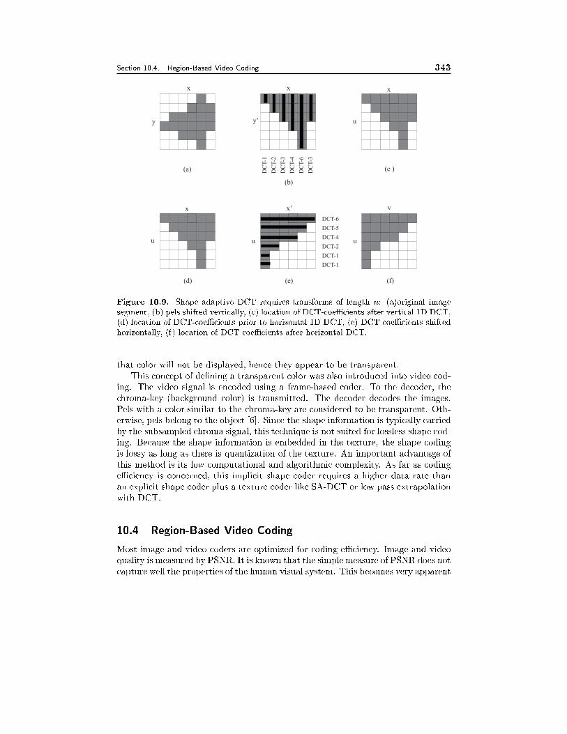
Section 10.4. Region-Based Video Coding 343
x
y
x
y’
x
x
u
u
x’
u
v
u
(a)
(b)
(d) (e) (f)
(c )DC
T-1
DC
T-2
DC
T-3
DC
T-4
DC
T-6
DC
T-3
DCT-6
DCT-5
DCT-4
DCT-2
DCT-1
DCT-1
Figure 10.9. Shape adaptive DCT requires transforms of length n: (a)original image
segment, (b) pels shifted vertically, (c) location of DCT-coeÆcients after vertical 1D DCT,
(d) location of DCT-coeÆcients prior to horizontal 1D DCT, (e) DCT coeÆcients shifted
horizontally, (f) location of DCT coeÆcients after horizontal DCT.
that color will not be displayed, hence they appear to be transparent.
This concept of de�ning a transparent color was also introduced into video cod-
ing. The video signal is encoded using a frame-based coder. To the decoder, the
chroma-key (background color) is transmitted. The decoder decodes the images.
Pels with a color similar to the chroma-key are considered to be transparent. Oth-
erwise, pels belong to the object [6]. Since the shape information is typically carried
by the subsampled chroma signal, this technique is not suited for lossless shape cod-
ing. Because the shape information is embedded in the texture, the shape coding
is lossy as long as there is quantization of the texture. An important advantage of
this method is its low computational and algorithmic complexity. As far as coding
eÆciency is concerned, this implicit shape coder requires a higher data rate than
an explicit shape coder plus a texture coder like SA-DCT or low pass extrapolation
with DCT.
10.4 Region-Based Video Coding
Most image and video coders are optimized for coding eÆciency. Image and video
quality is measured by PSNR. It is known that the simple measure of PSNR does not
capture well the properties of the human visual system. This becomes very apparent
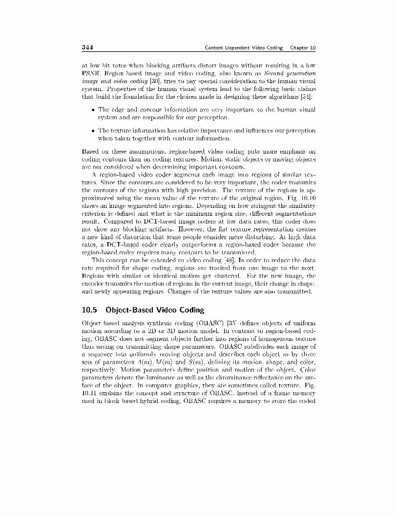
344 Content Dependent Video Coding Chapter 10
at low bit rates when blocking artifacts distort images without resulting in a low
PSNR. Region-based image and video coding, also known as Second generation
image and video coding [30], tries to pay special consideration to the human visual
system. Properties of the human visual system lead to the following basic claims
that build the foundation for the choices made in designing these algorithms [54]:
� The edge and contour information are very important to the human visual
system and are responsible for our perception.
� The texture information has relative importance and in uences our perception
when taken together with contour information.
Based on these assumptions, region-based video coding puts more emphasis on
coding contours than on coding textures. Motion, static objects or moving objects
are not considered when determining important contours.
A region-based video coder segments each image into regions of similar tex-
tures. Since the contours are considered to be very important, the coder transmits
the contours of the regions with high precision. The texture of the regions is ap-
proximated using the mean value of the texture of the original region. Fig. 10.10
shows an image segmented into regions. Depending on how stringent the similarity
criterion is de�ned and what is the minimum region size, di�erent segmentations
result. Compared to DCT-based image coders at low data rates, this coder does
not show any blocking artifacts. However, the at texture representation creates
a new kind of distortion that some people consider more disturbing. At high data
rates, a DCT-based coder clearly outperforms a region-based coder because the
region-based coder requires many contours to be transmitted.
This concept can be extended to video coding [48]. In order to reduce the data
rate required for shape coding, regions are tracked from one image to the next.
Regions with similar or identical motion get clustered. For the new image, the
encoder transmits the motion of regions in the current image, their change in shape,
and newly appearing regions. Changes of the texture values are also transmitted.
10.5 Object-Based Video Coding
Object-based analysis-synthesis coding (OBASC) [35] de�nes objects of uniform
motion according to a 2D or 3D motion model. In contrast to region-based cod-
ing, OBASC does not segment objects further into regions of homogenous texture
thus saving on transmitting shape parameters. OBASC subdivides each image of
a sequence into uniformly moving objects and describes each object m by three
sets of parameters A(m);M(m) and S(m), de�ning its motion, shape, and color,
respectively. Motion parameters de�ne position and motion of the object. Color
parameters denote the luminance as well as the chrominance re ectance on the sur-
face of the object. In computer graphics, they are sometimes called texture. Fig.
10.11 explains the concept and structure of OBASC. Instead of a frame memory
used in block based hybrid coding, OBASC requires a memory to store the coded
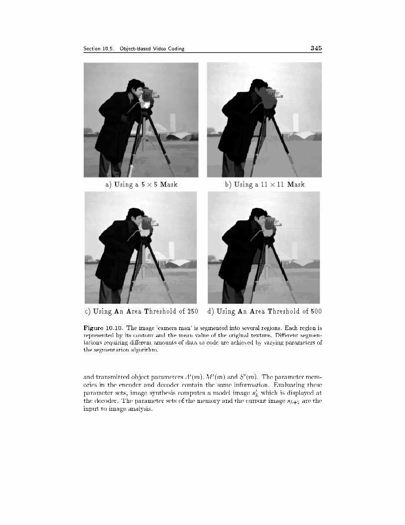
Section 10.5. Object-Based Video Coding 345
Figure 10.10. The image `camera man' is segmented into several regions. Each region is
represented by its contour and the mean value of the original texture. Di�erent segmen-
tations requiring di�erent amounts of data to code are achieved by varying parameters of
the segmentation algorithm.
and transmitted object parameters A0(m);M 0(m) and S0(m). The parameter mem-
ories in the encoder and decoder contain the same information. Evaluating these
parameter sets, image synthesis computes a model image s0k which is displayed at
the decoder. The parameter sets of the memory and the current image sk+1 are the
input to image analysis.
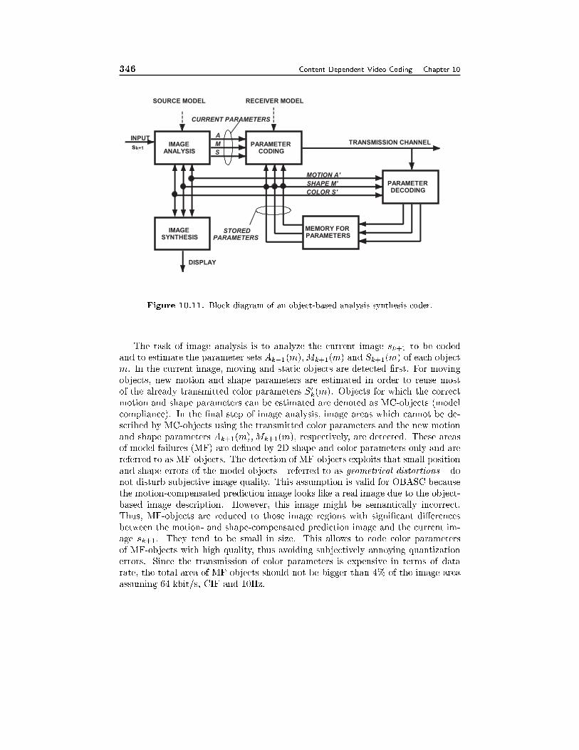
346 Content Dependent Video Coding Chapter 10
IMAGE
ANALYSIS
PARAMETER
CODING
IMAGE
SYNTHESIS
PARAMETER
DECODING
MEMORY FOR
PARAMETERS
MOTION A'
SHAPE M'
COLOR S'
TRANSMISSION CHANNEL
DISPLAY
STORED
PARAMETERS
CURRENT PARAMETERS
SOURCE MODEL RECEIVER MODEL
INPUT
sk+1
A
M
S
Figure 10.11. Block diagram of an object-based analysis synthesis coder.
The task of image analysis is to analyze the current image sk+1 to be coded
and to estimate the parameter sets Ak+1(m);Mk+1(m) and Sk+1(m) of each object
m. In the current image, moving and static objects are detected �rst. For moving
objects, new motion and shape parameters are estimated in order to reuse most
of the already transmitted color parameters S0k(m). Objects for which the correct
motion and shape parameters can be estimated are denoted as MC-objects (model
compliance). In the �nal step of image analysis, image areas which cannot be de-
scribed by MC-objects using the transmitted color parameters and the new motion
and shape parameters Ak+1(m);Mk+1(m), respectively, are detected. These areas
of model failures (MF) are de�ned by 2D-shape and color parameters only and are
referred to as MF-objects. The detection of MF-objects exploits that small position
and shape errors of the model objects - referred to as geometrical distortions - do
not disturb subjective image quality. This assumption is valid for OBASC because
the motion-compensated prediction image looks like a real image due to the object-
based image description. However, this image might be semantically incorrect.
Thus, MF-objects are reduced to those image regions with signi�cant di�erences
between the motion- and shape-compensated prediction image and the current im-
age sk+1. They tend to be small in size. This allows to code color parameters
of MF-objects with high quality, thus avoiding subjectively annoying quantization
errors. Since the transmission of color parameters is expensive in terms of data
rate, the total area of MF-objects should not be bigger than 4% of the image area
assuming 64 kbit/s, CIF and 10Hz.
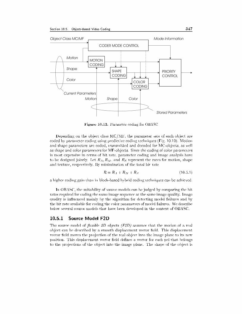
Section 10.5. Object-Based Video Coding 347
CODER MODE CONTROL
PRIORITY
CONTROL
MOTION
CODING
SHAPE
CODING
COLOR
CODING
Object Class MC/MF
Motion
Shape
Color
Mode Information
Current Parameters
Stored Parameters
Motion Shape Color
Figure 10.12. Parameter coding for OBASC
Depending on the object class MC/MF, the parameter sets of each object are
coded by parameter coding using predictive coding techniques (Fig. 10.12). Motion
and shape parameters are coded, transmitted and decoded for MC-objects, as well
as shape and color parameters for MF-objects. Since the coding of color parameters
is most expensive in terms of bit rate, parameter coding and image analysis have
to be designed jointly. Let RA; RM ; and RS represent the rates for motion, shape
and texture, respectively. By minimization of the total bit rate
R = RA +RM +RS (10.5.1)
a higher coding gain than in block-based hybrid coding techniques can be achieved.
In OBASC, the suitability of source models can be judged by comparing the bit
rates required for coding the same image sequence at the same image quality. Image
quality is in uenced mainly by the algorithm for detecting model failures and by
the bit rate available for coding the color parameters of model failures. We describe
below several source models that have been developed in the context of OBASC.
10.5.1 Source Model F2D
The source model of exible 2D objects (F2D) assumes that the motion of a real
object can be described by a smooth displacement vector �eld. This displacement
vector �eld moves the projection of the real object into the image plane to its new
position. This displacement vector �eld de�nes a vector for each pel that belongs
to the projections of the object into the image plane. The shape of the object is
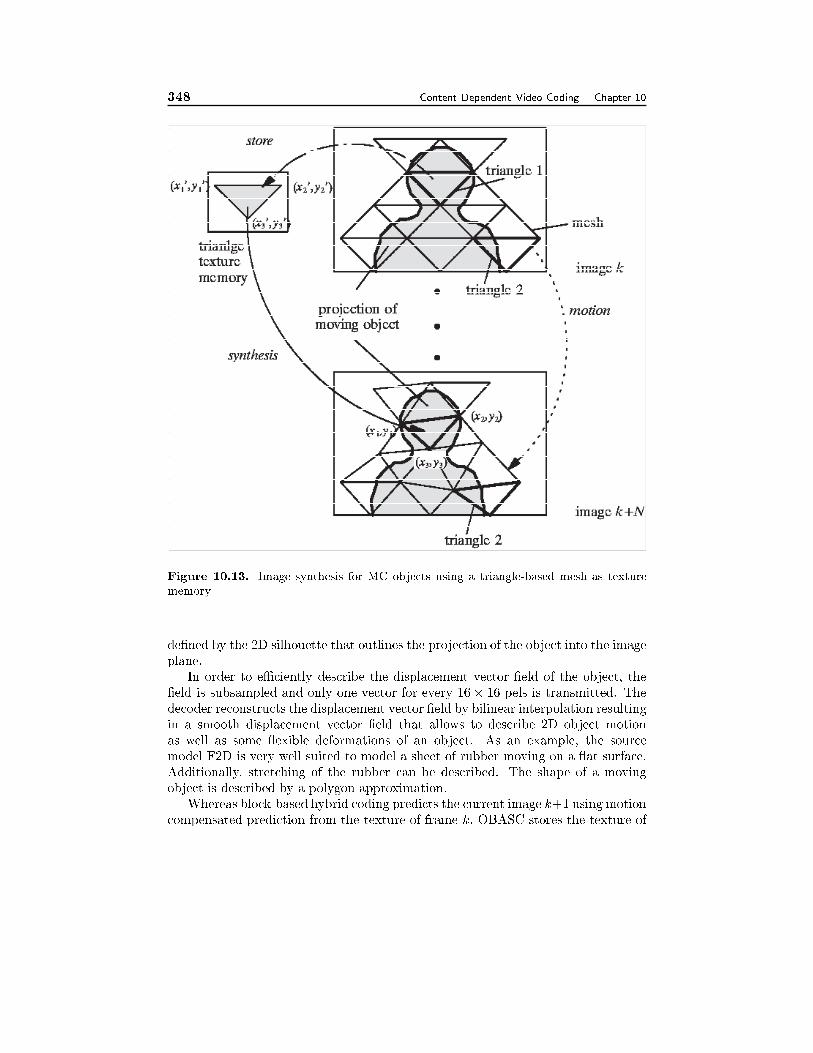
348 Content Dependent Video Coding Chapter 10
Figure 10.13. Image synthesis for MC objects using a triangle-based mesh as texture
memory
de�ned by the 2D silhouette that outlines the projection of the object into the image
plane.
In order to eÆciently describe the displacement vector �eld of the object, the
�eld is subsampled and only one vector for every 16� 16 pels is transmitted. The
decoder reconstructs the displacement vector �eld by bilinear interpolation resulting
in a smooth displacement vector �eld that allows to describe 2D object motion
as well as some exible deformations of an object. As an example, the source
model F2D is very well suited to model a sheet of rubber moving on a at surface.
Additionally, stretching of the rubber can be described. The shape of a moving
object is described by a polygon approximation.
Whereas block-based hybrid coding predicts the current image k+1 using motion
compensated prediction from the texture of frame k, OBASC stores the texture of
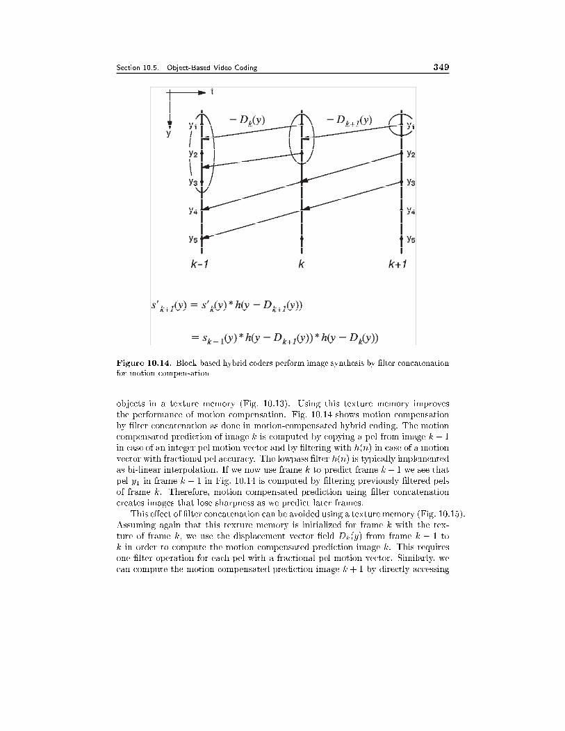
Section 10.5. Object-Based Video Coding 349
Figure 10.14. Block-based hybrid coders perform image synthesis by �lter concatenation
for motion compensation
objects in a texture memory (Fig. 10.13). Using this texture memory improves
the performance of motion compensation. Fig. 10.14 shows motion compensation
by �lter concatenation as done in motion-compensated hybrid coding. The motion
compensated prediction of image k is computed by copying a pel from image k � 1
in case of an integer pel motion vector and by �ltering with h(n) in case of a motion
vector with fractional pel accuracy. The lowpass �lter h(n) is typically implemented
as bi-linear interpolation. If we now use frame k to predict frame k+1 we see that
pel y1 in frame k + 1 in Fig. 10.14 is computed by �ltering previously �ltered pels
of frame k. Therefore, motion compensated prediction using �lter concatenation
creates images that lose sharpness as we predict later frames.
This e�ect of �lter concatenation can be avoided using a texture memory (Fig. 10.15).
Assuming again that this texture memory is initialized for frame k with the tex-
ture of frame k, we use the displacement vector �eld Dk(y) from frame k � 1 to
k in order to compute the motion compensated prediction image k. This requires
one �lter operation for each pel with a fractional pel motion vector. Similarly, we
can compute the motion compensated prediction image k + 1 by directly accessing
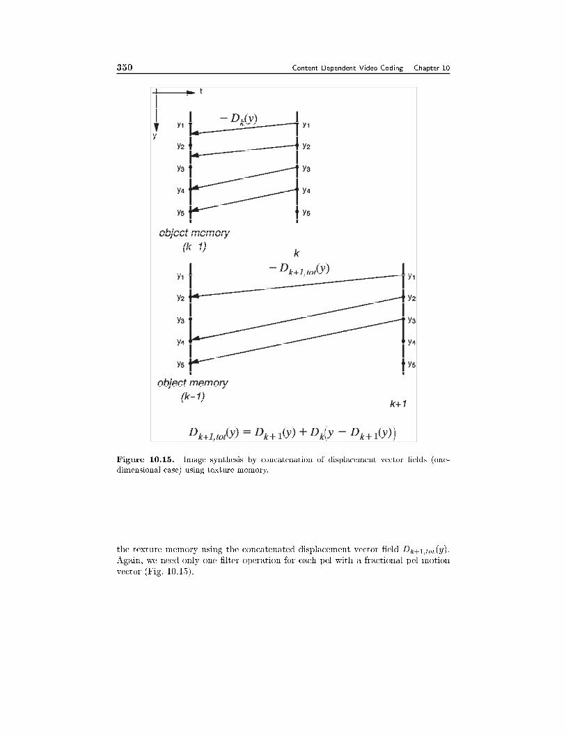
350 Content Dependent Video Coding Chapter 10
Figure 10.15. Image synthesis by concatenation of displacement vector �elds (one-
dimensional case) using texture memory.
the texture memory using the concatenated displacement vector �eld Dk+1;tot(y).
Again, we need only one �lter operation for each pel with a fractional pel motion
vector (Fig. 10.15).
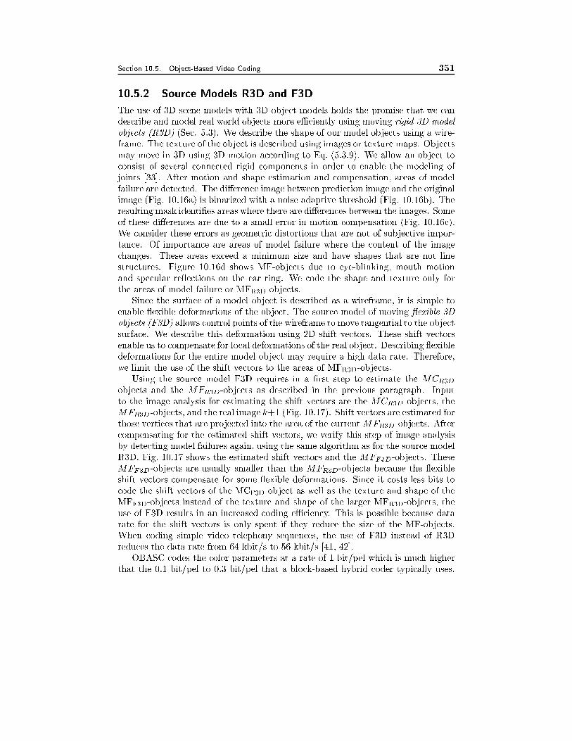
Section 10.5. Object-Based Video Coding 351
10.5.2 Source Models R3D and F3D
The use of 3D scene models with 3D object models holds the promise that we can
describe and model real world objects more eÆciently using moving rigid 3D model
objects (R3D) (Sec. 5.3). We describe the shape of our model objects using a wire-
frame. The texture of the object is described using images or texture maps. Objects
may move in 3D using 3D motion according to Eq. (5.3.9). We allow an object to
consist of several connected rigid components in order to enable the modeling of
joints [33]. After motion and shape estimation and compensation, areas of model
failure are detected. The di�erence image between prediction image and the original
image (Fig. 10.16a) is binarized with a noise adaptive threshold (Fig. 10.16b). The
resulting mask identi�es areas where there are di�erences between the images. Some
of these di�erences are due to a small error in motion compensation (Fig. 10.16c).
We consider these errors as geometric distortions that are not of subjective impor-
tance. Of importance are areas of model failure where the content of the image
changes. These areas exceed a minimum size and have shapes that are not line
structures. Figure 10.16d shows MF-objects due to eye-blinking, mouth motion
and specular re ections on the ear ring. We code the shape and texture only for
the areas of model failure or MFR3D objects.
Since the surface of a model object is described as a wireframe, it is simple to
enable exible deformations of the object. The source model of moving exible 3D
objects (F3D) allows control points of the wireframe to move tangential to the object
surface. We describe this deformation using 2D shift vectors. These shift vectors
enable us to compensate for local deformations of the real object. Describing exible
deformations for the entire model object may require a high data rate. Therefore,
we limit the use of the shift vectors to the areas of MFR3D-objects.
Using the source model F3D requires in a �rst step to estimate the MCR3Dobjects and the MFR3D-objects as described in the previous paragraph. Input
to the image analysis for estimating the shift vectors are the MCR3D objects, the
MFR3D-objects, and the real image k+1 (Fig. 10.17). Shift vectors are estimated for
those vertices that are projected into the area of the currentMFR3D-objects. After
compensating for the estimated shift vectors, we verify this step of image analysis
by detecting model failures again, using the same algorithm as for the source model
R3D. Fig. 10.17 shows the estimated shift vectors and the MFF3D-objects. These
MFF3D-objects are usually smaller than the MFR3D-objects because the exible
shift vectors compensate for some exible deformations. Since it costs less bits to
code the shift vectors of the MCF3D object as well as the texture and shape of the
MFF3D-objects instead of the texture and shape of the larger MFR3D-objects, the
use of F3D results in an increased coding eÆciency. This is possible because data
rate for the shift vectors is only spent if they reduce the size of the MF-objects.
When coding simple video telephony sequences, the use of F3D instead of R3D
reduces the data rate from 64 kbit/s to 56 kbit/s [41, 42].
OBASC codes the color parameters at a rate of 1 bit/pel which is much higher
that the 0.1 bit/pel to 0.3 bit/pel that a block-based hybrid coder typically uses.
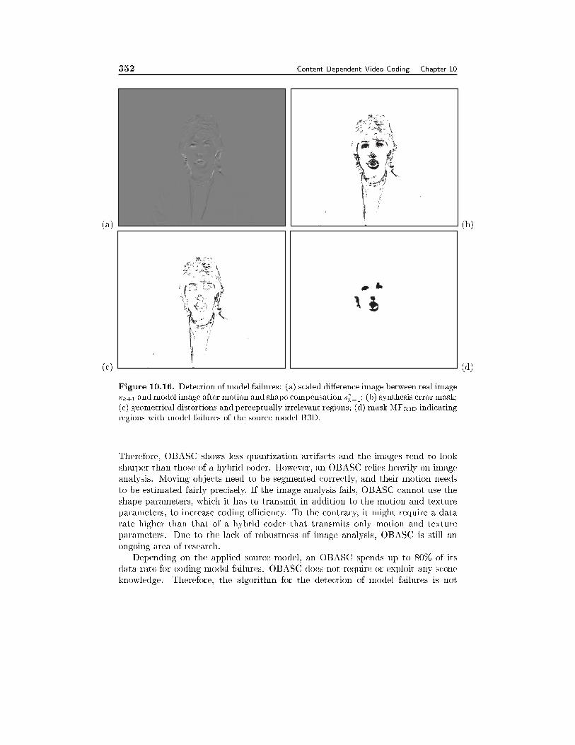
352 Content Dependent Video Coding Chapter 10
(a) (b)
(c) (d)
Figure 10.16. Detection of model failures: (a) scaled di�erence image between real image
sk+1 and model image after motion and shape compensation s�
k+1; (b) synthesis error mask;
(c) geometrical distortions and perceptually irrelevant regions; (d) mask MFR3D indicating
regions with model failures of the source model R3D.
Therefore, OBASC shows less quantization artifacts and the images tend to look
sharper than those of a hybrid coder. However, an OBASC relies heavily on image
analysis. Moving objects need to be segmented correctly, and their motion needs
to be estimated fairly precisely. If the image analysis fails, OBASC cannot use the
shape parameters, which it has to transmit in addition to the motion and texture
parameters, to increase coding eÆciency. To the contrary, it might require a data
rate higher than that of a hybrid coder that transmits only motion and texture
parameters. Due to the lack of robustness of image analysis, OBASC is still an
ongoing area of research.
Depending on the applied source model, an OBASC spends up to 80% of its
data rate for coding model failures. OBASC does not require or exploit any scene
knowledge. Therefore, the algorithm for the detection of model failures is not
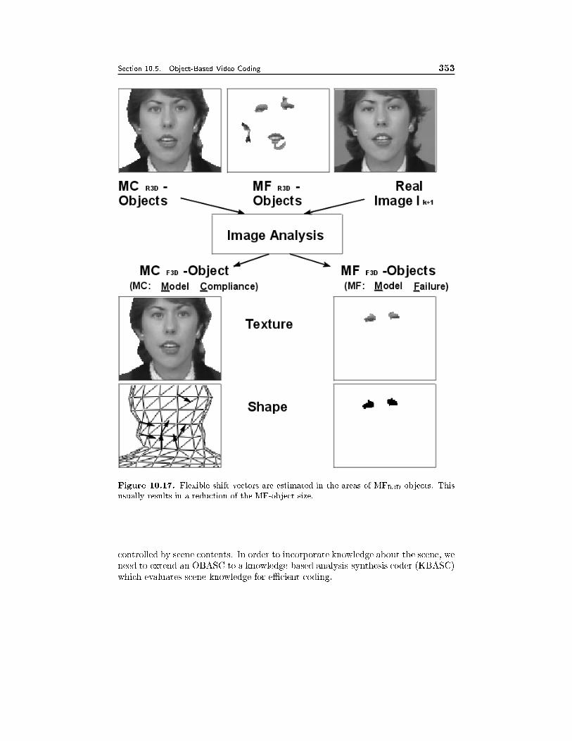
Section 10.5. Object-Based Video Coding 353
Figure 10.17. Flexible shift vectors are estimated in the areas of MFR3D-objects. This
usually results in a reduction of the MF-object size.
controlled by scene contents. In order to incorporate knowledge about the scene, we
need to extend an OBASC to a knowledge-based analysis-synthesis coder (KBASC)
which evaluates scene knowledge for eÆcient coding.
354 Content Dependent Video Coding Chapter 10
10.6 Knowledge-Based Video Coding
A knowledge-based analysis-synthesis coder (KBASC) is based on an OBASC. In
addition, the coder tries to recognize objects like faces in a video scene. As soon
as the coder recognizes an object, it switches the coding mode for the object from
the generic object-based mode to a knowledge-based mode. For head and shoulder
scenes, the goal is to achieve a better modelling of the human face and to use the
knowledge of the face location to control the coder. In order to enable an automatic
switching from an OBASC to a KBASC, an algorithm for recognizing facial features
and the adaptation of a face model to the image sequences is proposed [24]. First, we
need to identify eyes and mouth of the person that we want to code using KBASC
(Fig. 10.18a). In a second step , we need to adapt a face model into the wireframe
that currently represents the person (Fig. 10.18b). As an example, we incorporate
the face model Candide (Fig. 10.18c)[44] into the object model. We can adapt the
face model to the face of a person in an image by scaling the face model horizontally
to match the distance between the two eyes and vertically to match the distance
between mouth and eyes. Finally, we need to stitch the face model into the the
wireframe model that we use to describe the object when coding with the OBASC
layer (Fig. 10.18d).
As soon as KBASC has detected a face, its coding eÆciency increases com-
pared to OBASC. One reason is that the use of a face model instead of a generic
model improves the shape representation and allows for better motion compensa-
tion. Knowing the location of the face also allows to de�ne the joint between head
and shoulders more precisely, which again results in improved motion estimation
and compensation. Finally, we can use the knowledge about the face location to
compute model failures in a scene-dependent fashion. While we continue to use
a sensitive detection algorithm in the face area we can attribute most prediction
errors outside of the face area to geometric distortions as well as illumination errors
that we choose to neglect. In an experiment with the test sequence Claire at a
spatial resolution of 352x288 pels and frame rate of 10Hz, the average area of model
failures was 3% for the source model F3D. The area decreased to 2.7% when we
adapted the face model into the model object. Finally, exploiting the knowledge
of the face location for the detection of model failures reduced their area to 2.5%
without loss of subjective image quality. The corresponding data rates are 57 kbit/s
for F3D of the OBASC coder and 47 kbit/s for KBASC [24].
10.7 Semantic Video Coding
Previously described video coding algorithms describe each frame of a video se-
quence using a combination of the current image signal and a predicted image
signal that is derived using temporal prediction. Semantic video coding describes a
video sequence using model objects with behavior that represent real objects with
their behavior. We expect semantic coding to be far more eÆcient than the other
video coders because motion and deformation of most objects is very limited when
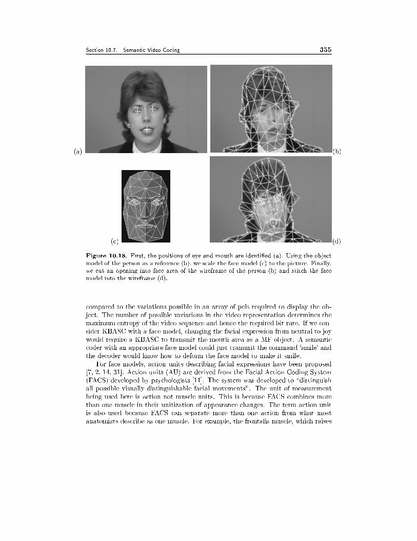
Section 10.7. Semantic Video Coding 355
(a) (b)
(c) (d)
Figure 10.18. First, the positions of eye and mouth are identi�ed (a). Using the object
model of the person as a reference (b), we scale the face model (c) to the picture. Finally,
we cut an opening into face area of the wireframe of the person (b) and stitch the face
model into the wireframe (d).
compared to the variations possible in an array of pels required to display the ob-
ject. The number of possible variations in the video representation determines the
maximum entropy of the video sequence and hence the required bit rate. If we con-
sider KBASC with a face model, changing the facial expression from neutral to joy
would require a KBASC to transmit the mouth area as a MF-object. A semantic
coder with an appropriate face model could just transmit the command `smile' and
the decoder would know how to deform the face model to make it smile.
For face models, action units describing facial expressions have been proposed
[7, 2, 14, 31]. Action units (AU) are derived from the Facial Action Coding System
(FACS) developed by psychologists [11]. The system was developed to \distinguish
all possible visually distinguishable facial movements". The unit of measurement
being used here is action not muscle units. This is because FACS combines more
than one muscle in their unitization of appearance changes. The term action unit
is also used because FACS can separate more than one action from what most
anatomists describe as one muscle. For example, the frontalis muscle, which raises
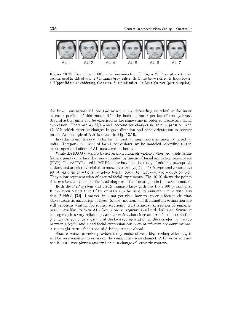
356 Content Dependent Video Coding Chapter 10
Figure 10.19. Examples of di�erent action units from [3, Figure 2]: Examples of the six
actions used in this study. AU 1: Inner brow raiser. 2: Outer brow raiser. 4: Brow lower.
5: Upper lid raiser (widening the eyes). 6: Cheek raiser. 7: Lid tightener (partial squint).
the brow, was separated into two action units, depending on whether the inner
or outer portion of this muscle lifts the inner or outer portion of the eyebrow.
Several action units can be exercised at the same time in order to create any facial
expression. There are 46 AUs which account for changes in facial expression, and
12 AUs which describe changes in gaze direction and head orientation in coarser
terms. An example of AUs is shown in Fig. 10.19.
In order to use this system for face animation, amplitudes are assigned to action
units. Temporal behavior of facial expressions can be modeled according to the
onset, apex and o�set of AU measured on humans.
While the FACS system is based on the human physiology, other proposals de�ne
feature points on a face that are animated by means of facial animation parameters
(FAP). The 68 FAPs used in MPEG-4 are based on the study of minimal perceptible
actions and are closely related to muscle actions [23][53]. FAPs represent a complete
set of basic facial actions including head motion, tongue, eye, and mouth control.
They allow representation of natural facial expressions. Fig. 10.20 shows the points
that can be used to de�ne the head shape and the feature points that are animated.
Both the FAP system and FACS animate faces with less than 100 parameters.
It has been found that FAPs or AUs can be used to animate a face with less
than 2 kbit/s [52]. However, it is not yet clear how to create a face model that
allows realistic animation of faces. Shape, motion, and illumination estimation are
still problems waiting for robust solutions. Furthermore, extraction of semantic
parameters like FAPs or AUs from a video sequence is a hard challenge. Semantic
coding requires very reliable parameter estimation since an error in the estimation
changes the semantic meaning of the face representation at the decoder. A mix-up
between a joyful and a sad facial expression can prevent e�ective communications.
A car might turn left instead of driving straight ahead.
Since a semantic coder provides the promise of very high coding eÆciency, it
will be very sensitive to errors on the communications channel. A bit error will not
result in a lower picture quality but in a change of semantic content.
Section 10.8. Layered Coding 357
10.8 Layered Coding
Depending on the scene content, it may not be eÆcient to describe each moving
object with a separate object model in an object-based coder. Similarly, it is not
always eÆcient to code an image of a sequence with a reference to previous images.
Hence, we need to code a video sequence with the appropriate set of source models.
In [34], a layered coder is proposed (Fig. 10.21). The layered coder allows the
application of di�erent source models and di�erent levels of scene understanding
for coding of an image sequence such that the best performance is guaranteed.
Whereas Layer I only transmits the color parameters of statistically dependent
pels, Layer II allows the additional transmission of motion parameters for blocks
of �xed size and position. Hence Layer I corresponds to an image coder or the
I-frame coder of an hybrid coder. Layer II corresponds to the coding of P-frames
in a hybrid coder. Layer III, the analysis-synthesis coder, allows the transmission
of shape parameters in order to describe arbitrarily shaped objects. Here, Layer
III is represented by an OBASC based on the source model of F3D. Using a 3D
source model allows for a seemless integration with KBASC. In layer IV, knowledge
of the scene contents is extracted from the video sequence and transmitted, in order
to apply scene dependent object models like the face model Candide. Layer V
transmits high-level symbols for describing complex behavior of the objects.
Whereas di�erent layers of this layered coder have been investigated by many
groups, the selection of the appropriate layer for encoding has been thoroughly
investigated only for layers I and II, since these layers correspond to coding blocks
in intra mode or predicitve mode in a block-based hybrid coder. The switching
between the layers II and III has only recently been addressed. In [8], a selection
depending on the residual coding error and bitrate is proposed. In [40], the size of
a moving object decides whether the object is coded in the block-based or in the
object-based layer. Switching between the OBASC of layer III and the KBASC of
layer IV is addressed in [24]. A semantic coder suitable for integration into a layered
coding system has been investigated in [13]. This coder saves 35% of the data rate
for coding head and shoulder video sequences when compared to the H.263 video
coder (Layer I and II).
10.9 Summary
In this chapter, we discussed content-based video coding, which describes individual
video objects and not just entire frames. In order to describe an object we use an
alpha-map that de�nes for each pel of a frame whether it belongs to the object
or not. In addition, the alpha-map allows to describe arbitrary transparency for
a video object. In order to eÆciently transmit the shape of an video object, we
looked at 2D shape coding algorithms. Bitmap-based shape coders describe for
each pel whether it belongs to the object using a context-based arithmetic coder,
contour-based coders describe the outline of an object using polygons, splines or a
chain code. The human visual system is relatively sensitive to shape distortions.
358 Content Dependent Video Coding Chapter 10
Therefore, we tend to code shapes with high quality.
As far as texture coding is concerned, we now need to be able to code the texture
of an arbitrarily shaped region. One possibility is to low-pass extrapolate the texture
such that it �lls a square block that can be coded using standard transform coders
like DCT. Alternatively, we can use the more eÆcient shape adaptive DCT or
wavelet transform that creates only as many coeÆcients as there are pels to be
coded.
Object-based analysis-synthesis coding (OBASC) integrates arbitrarily shaped
video objects into the framework of video coding. Since an object is now described
as a unit, the motion-compensated prediction image looks like a natural image. It
does not su�er from the block distortion of the block-based motion-compensated
prediction images. We use the concept of model failures to determine those parts
of an image that cannot be modeled with suÆcient subjective quality. OBASC has
been implemented using 2D and 3D source models. 3D source models were extended
to knowledge-based coding where the coder identi�es prede�ned models like faces to
describe the video scene more eÆciently. Semantic coding aims at describing video
using high-level descriptions. It is mainly developed for faces where parameter sets
like AU or FAP are used to animate a face.
Finally, we looked at a layered coder that integrates di�erent coding modes into
a framework. The layered coder switches from one coder to another based on the
coding eÆciency ensuring that we always code a video scene with the most eÆcient
source model.
EÆcient content-dependent video coding depends on an image analysis that
describes the image content accurately. Image analysis includes the problems of
segmenting the objects or regions and estimating their motion. Segmentation in-
volves partition of an initial video frame into regions of coherent texture or motion,
and the tracking of these regions over time. In Sec. 6.8, we brie y considered the
problem of segmenting a frame into regions of coherent motion. There we have
seen that motion estimation and region segmentation are inter-related and should
be jointly optimized. A more substantial discussion of segmentation and tracking
algorithms is beyond the scope of this book. Interested readers can explore this
topic further starting with these references [43][1][46][51].
10.10 Problems
10.1 What is an alpha-map and how is it used in video?
10.2 What are the 2 main shape coding approaches. Discuss their advantages and
disadvantages. How do they di�er when a shape is coded lossily?
10.3 What objective measures for shape quality do you know?
10.4 Imagine a diagonal line of one pel width. How does the representation of this
line change if we de�ne an object using pels with 4 or 8 neighbors? What is
the advantage of an hexagonal grid for pels?

Section 10.10. Problems 359
10.5 For the example given in Fig. 10.4, what are the direct chain code and the
di�erential chain code with 4-neighbors?
10.6 For the shape given in Fig. 10.22, derive the quad-tree representation.
10.7 For the Fourier descriptor representation of a contour given in Eq. (10.1.8),
prove that i) a translation of the contour will only in uence coeÆcient Z(0),
the DC value; ii) a scaling of the contour will multiply all coeÆcients with
the scale factor; and iii) a rotation of the contour will shift the phase of the
Fourier coeÆcients but it will not a�ect their amplitude.
10.8 Explain algorithms for joint shape and texture coding. What method is com-
monly used on the Internet?
10.9 How can you extend a pel-wise shape coder to work eÆciently not only in an
image coder but also in a video coder?
10.10 What approaches to texture coding of arbitrarily shaped objects do you
know? Compare their eÆciency.
10.11 What are the two main assumptions that guided the design of region-based
coders.
10.12 How do object-based analysis synthesis coding and region-based coding dif-
fer? Which coder will do better for natural video sequences and which for
cartoons? Explain.
10.13 What are the most commonly used source models for OBASC?
10.14 Model failure detection ignores geometrical distortions. What are they and
will they accumulate over time?
10.15 Explain image synthesis by �lter concatenation and image synthesis by dis-
placement vector �eld concatenation. Which method is more eÆcient?
10.16 Name at least 2 reasons why a knowledge-based coder can code a scene more
eÆciently than an OBASC?
10.17 Why does semantic coding hold the promise to be a very eÆcient coder.
Why do we not have semantic coders today?
10.18 What are the di�erences between action units and facial animation parame-
ters?
10.19 Explain the layers of a layered coder. Which layers are commonly used
today?
360 Content Dependent Video Coding Chapter 10
10.11 Bibliography
[1] T. Aach and A. Kaup. Bayesian algorithms for change detection in image se-
quences using markov random �elds. Signal Processing: Image Communication,
7(2):147{160, August 1995.
[2] K. Aizawa, H. Harashima, and T. Saito. Model-based analysis-synthesis image
coding (MBASIC) system for a person's face. Signal Processing: Image Commun.,
1(2), October 1989.
[3] M.S. Bartlett, P. A. Viola, T. J. Sejnowski, B.A. Golomb, J. Larsen, J. C.
Hager, and P. Ekman. Classifying facial action. In D. Touretzki, M. Mozer, and
M. Hasselmo, editors, Advances in Neural Information Processing Systems 8, pages
823{829. MIT Press, Cambridge, MA, 1996.
[4] G. Born. The File Formats Handbook. International Thomson Computer Press,
1995.
[5] N. Brady and F. Bossen. Shape compression of moving objects using context-
based arithmetic encoding. Signal Processing: Image Communications, 15(7-
8):601{617, May 2000.
[6] T. Chen, C. T. Swain, and B. G. Haskell. Coding of subregions for content-
based scalable video. IEEE Trans. On Circuits and Systems for video technology,
7:256{260, February 1997.
[7] C. S. Choi, K. Aizawa, H. Harashima, and T. Takebe. Analysis and synthesis of
facial image sequences in model-based image coding. IEEE trans on circuits and
systems for video technology, 4(3):257{275, June 1994.
[8] M.F. Chowdury, A.F. Clark, A.C. Downton, E. Morimatsu, and D.E. Pearson.
A switched model-based coder for video signals. IEEE Trans. on Circuits and
Systems for Video Technology, 4(3):216{227, June 1994.
[9] Compuserve. Graphics interchange format (sm), version 89a. Technical report,
CompuServe Incorporated, Columbus, Ohio, July 1990.
[10] M. de Klerk, R. Prasad, J.H. Bons, and N.B.J. Weyland. Introducing high-
resolution line graphics, in UK teletext using di�erential chain coding. IEE Pro-
ceedings I, 137(6):325{334, 1990.
[11] P. Eckman and V.W. Friesen. Facial coding system. Consulting Psychologists
Press Inc., Palo Alto, CA, USA, 1977.
[12] M. Eden and M. Kocher. On the performance of a contour coding algorithm in
the context of image coding. part i: Contour segment coding. Signal Processing,
8:381{386, 1985.

Section 10.11. Bibliography 361
[13] P. Eisert, T. Wiegand, and B. Girod. Model-aided coding: A new approach to
incorporate facial animation into motion-compensated video coding. IEEE Trans-
actions on Circuits and Systems for Video Technology, 10(3):344{358, April 2000.
[14] R. Forchheimer, O. Fahlander, and T. Kronander. A semantic approach to
the transmission of face images. In Proc. International Picture Coding Symposium
PCS`84, page 10.5, July 1984.
[15] H. Freeman. On the encoding of arbitrary geometric con�gurations. IRE Trans.
Electronic Computers, EC-10(2):260{268, June 1961.
[16] P. Gerken. Object-based analysis-synthesis coding of image sequences at very
low bit rates. IEEE Trans. Circuits and Systems for Video Technology, 4:228{235,
June 1994.
[17] M. Gilge, T. Engelhardt, and R. Mehlan. Coding of arbitrarely shaped image
segments based on a generalized orthogonal transform. EURASIP, Image Com-
munications, 1(2):153{180, October 1989.
[18] M. H�otter. Object-oriented analysis-synthesis coding based on two dimensional
objects. Signal Processing: Image Communication, 2(4):409{428, December 1990.
[19] M. H�otter. Optimization and eÆciency of an object-oriented analysis-synthesis
coder. IEEE Transactions on Circuits and Systems for video technology, 4(2):181{
194, April 1994.
[20] ITU-T. Recommendation T.6: Facsimile coding schemes and coding control
functions for group 4 facsimile apparatus, 1988.
[21] ITU-T. Recommendation T.82 (03/93) - information technology - coded repre-
sentation of picture and audio information - progressive bi-level image compression,
1993. (JBIG).
[22] A. K. Jain. Fundamentals of Digital Image Processing. Prentice Hall, 1989.
[23] P. Kalra, A. Mangili, N. Magnenat-Thalmann, and D. Thalmann. Simula-
tion of facial muscle actions based on rational free form deformations. In Proc.
Eurographics, pages 59{69, 1992.
[24] M. Kampmann and J. Ostermann. Automatic adaptation of a face model in a
layered coder with an object-based analysis-synthesis layer and a knowledge-based
layer. Signal Processing: Image Communications, 9(3):201{220, March 1997.
[25] T. Kaneko and M. Okudaira. Encoding of arbitrary curves based on the chain
code representation. Commun, 33:697{707, 1985.
[26] A.K. Katsaggelos, L.P. Kondi, F.W. Meier, J. Ostermann, and G.M. Schuster.
MPEG-4 and rate distortion based shape coding techniques. Proceedings of the
IEEE, Special issue on Multimedia Signal Processing, Part two, 86(6):1126{1154,
June 1998.
362 Content Dependent Video Coding Chapter 10
[27] A. Kaup. A new approach towards description of arbitrarily shaped image
segments. In Proc. SPIE Conf. Visual Communications and Image Processing
'97, SPIE Vol. 3012, pages 731{741, February 1997.
[28] J.I. Kim, A.C. Bovik, and B.L. Evans. Generalized predictive binary shape
coding using polygon approximation. SP:IC, 15(7-8):643{663, May 2000.
[29] J. Koplowitz. On the performance of chain codes for quantization of line draw-
ings. IEEE Trans. Pattern Anal. Machine Intell., 3(2):180{185, March 1981.
[30] M. Kunt, A. Ikonomopoulos, and M. Kocher. Second-generation image-coding
techniques. Proceedings of the IEEE, 73, pp. 549-574, April 1985.
[31] H. Li, P. Roivainen, and R. Forchheimer. 3-d motion estimation in model-based
facial image coding. IEEE Trans. Pattern Anal. Machine Intell., 15(6):545{555,
June 1993.
[32] S. Li and W. Li. Shape-adaptive discrete wavelet transforms for arbitrarily
shaped visual object coding. IEEE Trans. on Circuits, Systems, and Video Tech-
nology, 10(5):725{743, August 2000.
[33] G. Martinez. Shape estimation of articulated 3D objects for object-based
analysis-synthesis coding (OBASC). Signal Processing: Image Communication,
9(3):175{99, March 1997.
[34] H. Musmann. A layered coding system for very low bit rate video coding.
Signal Processing: Image Communication, 7(4-6):267{278, November 1995.
[35] H. G. Musmann, M. Hotter, and J. Ostermann. Object oriented analysis-
synthesis coding of moving images. Signal Processing: Image Commun., 1:119{138,
Oct. 1989.
[36] A. N. Netravali and B. G. Haskell. Digital Pictures { Representation and
Compression. Plenum Press, 1988.
[37] D.L. Neuho� and K.G. Castor. A rate and distortion analysis of chain codes
for line drawings. IEEE Transactions on Information Theory, 31(1):53{67, 1985.
[38] P. Nunes, F. Pereira, and F. Marques. Multi-grid chain coding of binary shapes.
In ICIP97, pages III:114{xx, 1997.
[39] K.J. O'Connell. Object-adaptive vertex-based shape coding method. IEEE
Transactions on Circuits and Systems, 7(1):251{255, February 1997.
[40] J. Ostermann. The block-based coder mode in an object-based analysis-
synthesis coder. In 28th Asilomar Conference on Signals, Systems, and Computers,
pages TP 6{1, November 1994.
Section 10.11. Bibliography 363
[41] J. Ostermann. Object-based analysis-synthesis coding based on the source
model of moving rigid 3D objects. Signal Processing: Image Communication,
2(6):143{161, 1994.
[42] J. Ostermann. Segmentation of image areas changed due to object motion
considering shadows. In Y. Wang et al., editor, Multimedia communications and
video coding, pages 241{246. Plenum Press, New York, 1996.
[43] W. K. Pratt. Digital Image Processing. John Wiley & Sons, 2nd ed. edition,
1991.
[44] R. Rydfalk. Candide, a parameterised face. Internal Report Lith{ISY{I{0866,
Link�oping University, Link�oping, Sweden, 1987.
[45] J.A. Saghri and H. Freeman. Analysis of the precision of generalized chain
codes for the representation of planar curves. IEEE Trans. Pattern Anal. Machine
Intell., 3(5):533{539, September 1981.
[46] P. Salembier and F. Marques. Region-based representations of image and video:
segmentation tools for multimedia services. IEEE Transactions on Circuits and
Systems for Video Technology, 9(8):1147{1169, December 1999.
[47] P. Salembier, F. Marques, and A. Gasull. Coding of partition sequences. In
L. Torres and M. Kunt, editors, Video Coding, pages 125{170. Kluwer Academic
Publishers, 1996.
[48] P. Salembier, L. Torres, F. Meyer, and C. Gu. Region-based video coding using
mathematical morphology. Proceedings of the IEEE, Special Issue on Digital TV,
83(6):843{857, June 1995.
[49] G.M. Schuster and A.G. Katsaggelos. An optimal segmentation encoding
scheme in the rate-distortion sense. In Proceedings of ISCAS 96, Atlanta, vol-
ume 2, pages 640{643, 1996.
[50] T. Sikora, S. Bauer, and B. Makai. EÆciency of shape-adaptive transforms
for coding of arbitrarily shaped image segments. IEEE Trans. on Circuits and
Systems for Video Technology, 5(3):254{8, June 1995.
[51] J. Stauder, R. Mech, and J. Ostermann. Detection of moving cast shadows for
object segmentation. IEEE Transactions on Multimedia, 1(1):65{76, March 1999.
[52] A. M. Tekalp and J. Ostermann. Face and 2-D mesh animation in MPEG-4.
Signal Processing: Image Communication, Special Issue on MPEG-4, 15:387{421,
January 2000.
[53] D. Terzopolous and K. Waters. Physically-based facial modeling, analysis and
animation. Jou. of Visualization and Computer Animation, 1:73{80, 1990.

364 Content Dependent Video Coding Chapter 10
[54] L. Torres and M. Kunt. Second generation video coding techniques, chapter 1,
pages 1{30. Kluwer Academic Publishers, Boston, MA, 1996.
[55] P. van Otterloo. A contour-oriented approach for shape analysis. Prentice Hall
International (UK), 1991.
[56] C.T. Zahn and R.Z. Roskies. Fourier descriptors for plane closed curves. IEEE
Transactions on Computer, 21(3):269{281, March 1972.
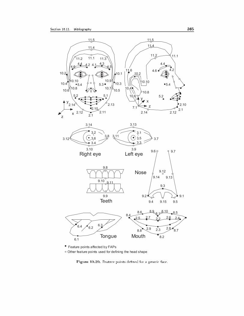
Section 10.11. Bibliography 365
xy
z
11.5
11.4
11.2
10.2
10.4
10.10
10.810.6
2.14
7.1
11.6 4.6
4.4
4.2
5.2
5.4
2.10
2.122.1
11.1
Tongue
6.26.4 6.3
6.1Mouth
8.18.9 8.10 8.5
8.7
8.2
8.8
8.48.6
2.2
2.3
2.6
2.82.9
2.72.5 2.4
2.12.12 2.11
2.142.10
2.13
10.610.8
10.4
10.2
10.105.4
5.2
5.3
5.1
10.1
10.910.3
10.510.7
4.1 4.34.54.6
4.4 4.2
11.111.2 11.3
11.4
11.5
x
y
z
Nose
9.6 9.7
9.14 9.13
9.12
9.2
9.4 9.15 9.5
9.3
9.1
Teeth
9.109.11
9.8
9.9
Feature points affected by FAPs
Other feature points used for defining the head shape
Right eye Left eye
3.13
3.7
3.9
3.5
3.1
3.3
3.11
3.14
3.10
3.12 3.6
3.4
3.23.8
Figure 10.20. Feature points de�ned for a generic face.
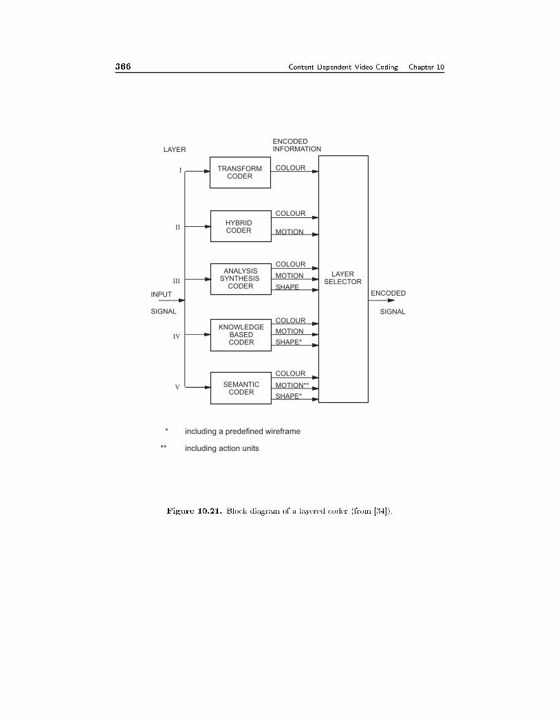
366 Content Dependent Video Coding Chapter 10
KNOWLEDGEBASEDCODER
ANALYSISSYNTHESIS
CODER
HYBRIDCODER
SEMANTICCODER
TRANSFORMCODER
LAYERSELECTOR
COLOUR
MOTION
SHAPE
COLOUR
MOTION
COLOUR
MOTION
SHAPE*
COLOUR
MOTION**
SHAPE*
COLOUR
ENCODED
SIGNAL
ENCODEDINFORMATION
INPUT
SIGNAL
I
II
IV
V
III
LAYER
* including a predefined wireframe
** including action units
Figure 10.21. Block diagram of a layered coder (from [34]).
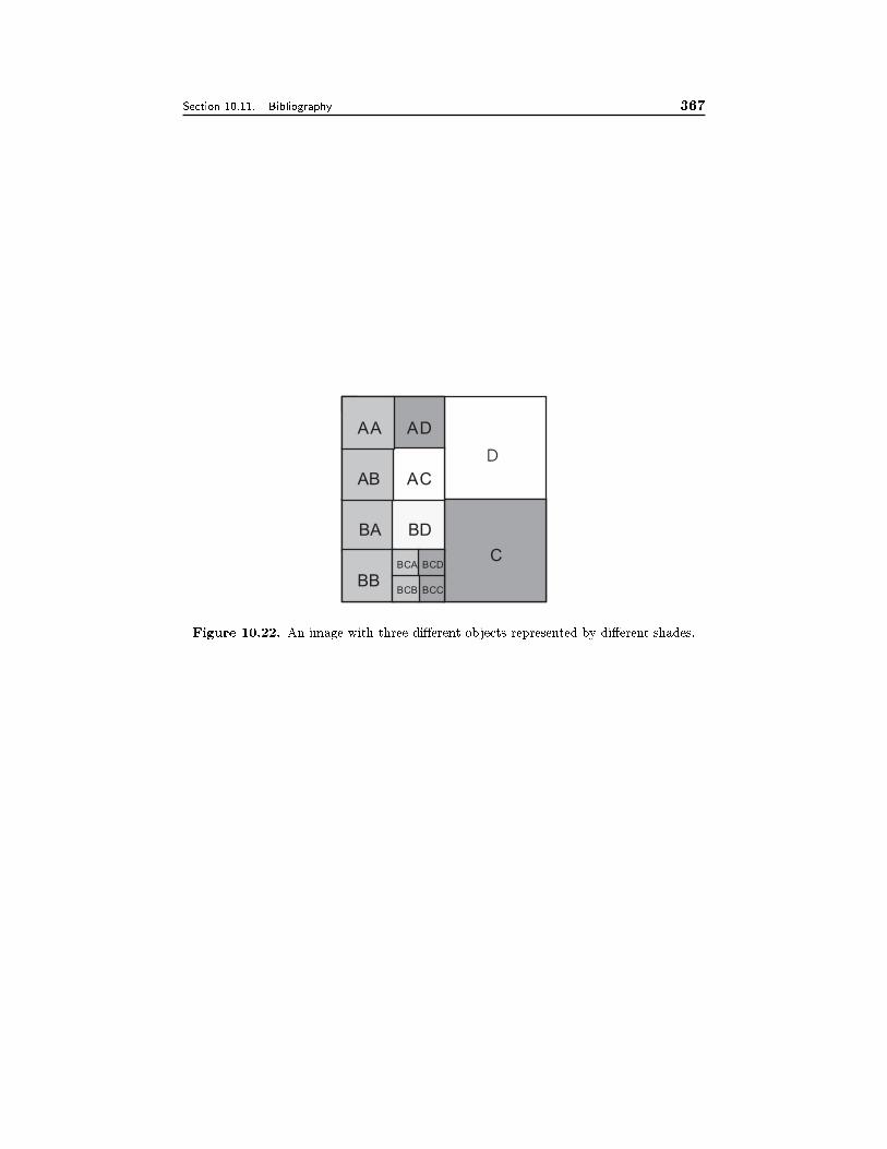
Section 10.11. Bibliography 367
A
BB
BA BD
AA
AB AC
AD
BCA
BCB BCC
BCDC
D
Figure 10.22. An image with three di�erent objects represented by di�erent shades.
Chapter 11
SCALABLE VIDEO CODING
The coding methods introduced in the previous chapters, including both waveform-
based and content-dependent methods, aim to optimize the coding eÆciency for
a �xed bit rate. This presents a diÆculty when multiple users try to access the
same video through di�erent communication links. For example, a MPEG-1 video
coded at 1.5 Mbps can be downloaded in real-time for play back in a terminal that
is connected to the server via a high-speed link (e.g., an ADSL modem). But a
user with only a modem connection of 56 Kbps will not be able to receive suÆcient
number of bits in time for playback in real-time. Scalability refers to the capabil-
ity of recovering physically meaningful image or video information from decoding
only partial compressed bitstreams. In the previous example, if the video stream
is scalable, then the user with high bandwidth connection can download the entire
bitstream to view the full quality video, while the user with 56 Kbps connection
will only download a subset of the stream, and see a low quality presentation.
The above example only illustrates one aspect of scalability: the bandwidth
scalability. A scalable stream can also o�er adaptivity to varying channel error
characteristics and computing powers at the receiving terminal. For wireless com-
munications, scalability allows adjusting the source rate and applying unequal error
protection in response to channel error conditions. For Internet transmission, scala-
bility enables variable bit rate transmission, selective bits discarding, and adjusting
source rate corresponding to di�erent modem rates, changing channel bandwidth,
and diverse device capabilities. As we move to the convergence of wireless, inter-
net and multimedia, scalability becomes increasingly important for compelling rich
media access to anywhere, by anyone, at anytime, with any device, and in any form.
Scalable coders can have coarse granularity (two or three layers, also called
layered coders), or �ne granularity. In the extreme case of �ne granularity, the
bit stream can be truncated at any point. The more bits are retained, the better
will be the reconstructed image quality. We call such type of bitstream embedded.
Embedded coders enable precise bitrate control, which is a desirable feature in many
applications. For example, network �lters (described later in Section 15.4.1) can
select the number of bits to transmit from an embedded bit-stream to match the
available bandwidth.
Scalable coding is typically accomplished by providing multiple versions of a
368
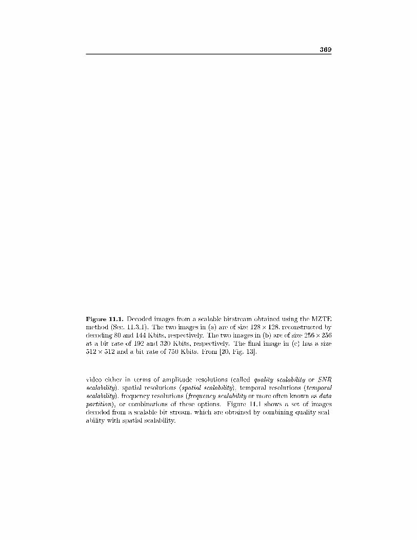
369
Figure 11.1. Decoded images from a scalable bitstream obtained using the MZTE
method (Sec. 11.3.1). The two images in (a) are of size 128� 128, reconstructed by
decoding 80 and 144 Kbits, respectively. The two images in (b) are of size 256�256
at a bit rate of 192 and 320 Kbits, respectively. The �nal image in (c) has a size
512� 512 and a bit rate of 750 Kbits. From [20, Fig. 13].
video either in terms of amplitude resolutions (called quality scalability or SNR
scalability), spatial resolutions (spatial scalability), temporal resolutions (temporal
scalability), frequency resolutions (frequency scalability or more often known as data
partition), or combinations of these options. Figure 11.1 shows a set of images
decoded from a scalable bit stream, which are obtained by combining quality scal-
ability with spatial scalability.
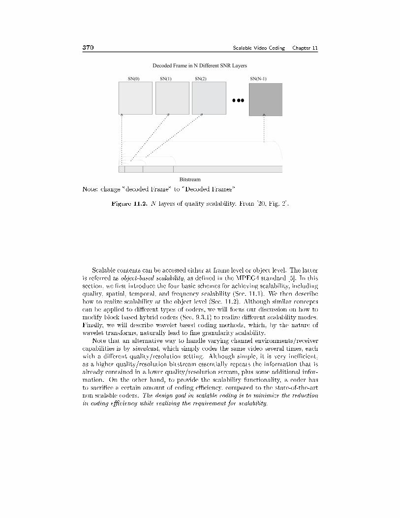
370 Scalable Video Coding Chapter 11
Bitstream
Decoded Frame in N Different SNR Layers
SN(0) SN(1) SN(2) SN(N-1)
Note: change "decoded Frame" to "Decoded Frames"
Figure 11.2. N layers of quality scalability. From [20, Fig. 2].
Scalable contents can be accessed either at frame level or object level. The latter
is referred as object-based scalability, as de�ned in the MPEG4 standard [5]. In this
section, we �rst introduce the four basic schemes for achieving scalability, including
quality, spatial, temporal, and frequency scalability (Sec. 11.1). We then describe
how to realize scalability at the object level (Sec. 11.2). Although similar concepts
can be applied to di�erent types of coders, we will focus our discussion on how to
modify block-based hybrid coders (Sec. 9.3.1) to realize di�erent scalability modes.
Finally, we will describe wavelet-based coding methods, which, by the nature of
wavelet transforms, naturally lead to �ne granularity scalability.
Note that an alternative way to handle varying channel environments/receiver
capabilities is by simulcast, which simply codes the same video several times, each
with a di�erent quality/resolution setting. Although simple, it is very ineÆcient,
as a higher quality/resolution bitstream essentially repeats the information that is
already contained in a lower quality/resolution stream, plus some additional infor-
mation. On the other hand, to provide the scalability functionality, a coder has
to sacri�ce a certain amount of coding eÆciency, compared to the state-of-the-art
non-scalable coders. The design goal in scalable coding is to minimize the reduction
in coding eÆciency while realizing the requirement for scalability.
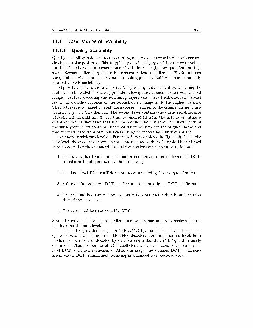
Section 11.1. Basic Modes of Scalability 371
11.1 Basic Modes of Scalability
11.1.1 Quality Scalability
Quality scalability is de�ned as representing a video sequence with di�erent accura-
cies in the color patterns. This is typically obtained by quantizing the color values
(in the original or a transformed domain) with increasingly �ner quantization step-
sizes. Because di�erent quantization accuracies lead to di�erent PSNRs between
the quantized video and the original one, this type of scalability is more commonly
referred as SNR scalability.
Figure 11.2 shows a bitstream with N layers of quality scalability. Decoding the
�rst layer (also called base layer) provides a low quality version of the reconstructed
image. Further decoding the remaining layers (also called enhancement layers)
results in a quality increase of the reconstructed image up to the highest quality.
The �rst layer is obtained by applying a coarse quantizer to the original image or in a
transform (e.g., DCT) domain. The second layer contains the quantized di�erence
between the original image and that reconstructed from the �rst layer, using a
quantizer that is �ner than that used to produce the �rst layer. Similarly, each of
the subsequent layers contains quantized di�erence between the original image and
that reconstructed from previous layers, using an increasingly �ner quantizer.
An encoder with two-level quality scalability is depicted in Fig. 11.3(a). For the
base level, the encoder operates in the same manner as that of a typical block-based
hybrid coder. For the enhanced level, the operations are performed as follows:
1. The raw video frame (or the motion compensation error frame) is DCT-
transformed and quantized at the base level;
2. The base-level DCT coeÆcients are reconstructed by inverse quantization;
3. Subtract the base-level DCT coeÆcients from the original DCT coeÆcient;
4. The residual is quantized by a quantization parameter that is smaller than
that of the base level;
5. The quantized bits are coded by VLC.
Since the enhanced level uses smaller quantization parameter, it achieves better
quality than the base level.
The decoder operation is depicted in Fig. 11.3(b). For the base level, the decoder
operates exactly as the non-scalable video decoder. For the enhanced level, both
levels must be received, decoded by variable length decoding (VLD), and inversely
quantized. Then the base-level DCT coeÆcient values are added to the enhanced-
level DCT coeÆcient re�nements. After this stage, the summed DCT coeÆcients
are inversely DCT-transformed, resulting in enhanced-level decoded video.
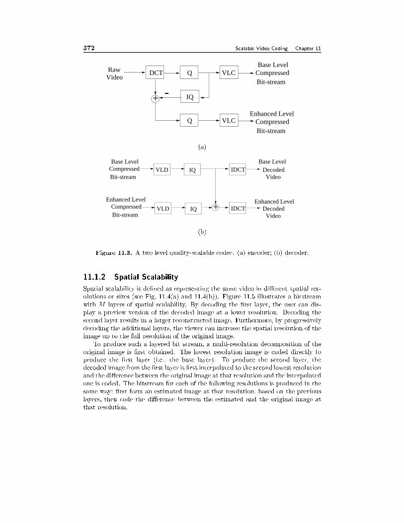
372 Scalable Video Coding Chapter 11
IQ
VideoRaw
+
Q
DCT Q VLC
VLC
Bit-streamCompressed
-Bit-streamCompressedBase Level
Enhanced Level
(a)
+ IDCT
IDCT
IQVLD
IQVLD
Bit-streamCompressed
Enhanced Level
Bit-streamCompressedBase Level
Video
Base Level
VideoDecoded
Decoded
Enhanced Level
(b)
Figure 11.3. A two level quality-scalable codec. (a) encoder; (b) decoder.
11.1.2 Spatial Scalability
Spatial scalability is de�ned as representing the same video in di�erent spatial res-
olutions or sizes (see Fig. 11.4(a) and 11.4(b)). Figure 11.5 illustrates a bitstream
with M layers of spatial scalability. By decoding the �rst layer, the user can dis-
play a preview version of the decoded image at a lower resolution. Decoding the
second layer results in a larger reconstructed image. Furthermore, by progressively
decoding the additional layers, the viewer can increase the spatial resolution of the
image up to the full resolution of the original image.
To produce such a layered bit stream, a multi-resolution decomposition of the
original image is �rst obtained. The lowest resolution image is coded directly to
produce the �rst layer (i.e., the base layer). To produce the second layer, the
decoded image from the �rst layer is �rst interpolated to the second lowest resolution
and the di�erence between the original image at that resolution and the interpolated
one is coded. The bitstream for each of the following resolutions is produced in the
same way: �rst form an estimated image at that resolution, based on the previous
layers, then code the di�erence between the estimated and the original image at
that resolution.
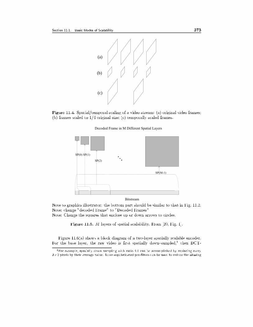
Section 11.1. Basic Modes of Scalability 373
(b)
(c)
(a)
Figure 11.4. Spatial/temporal scaling of a video stream: (a) original video frames;
(b) frames scaled to 1/4 original size; (c) temporally scaled frames.
SP(0) SP(1)
SP(2)
SP(M-1)
Bitstream
Decoded Frame in M Different Spatial Layers
Note to graphics illustrator: the bottom part should be similar to that in Fig. 11.2.
Note: change "decoded Frame" to "Decoded Frames"
Note: Change the squares that enclose up or down arrows to circles.
Figure 11.5. M layers of spatial scalability. From [20, Fig. 1].
Figure 11.6(a) shows a block diagram of a two-layer spatially scalable encoder.
For the base layer, the raw video is �rst spatially down-sampled,1 then DCT-
1For example, spatially down-sampling with ratio 4:1 can be accomplished by replacing every
2�2 pixels by their average value. More sophisticated pre-�lters can be used to reduce the aliasing
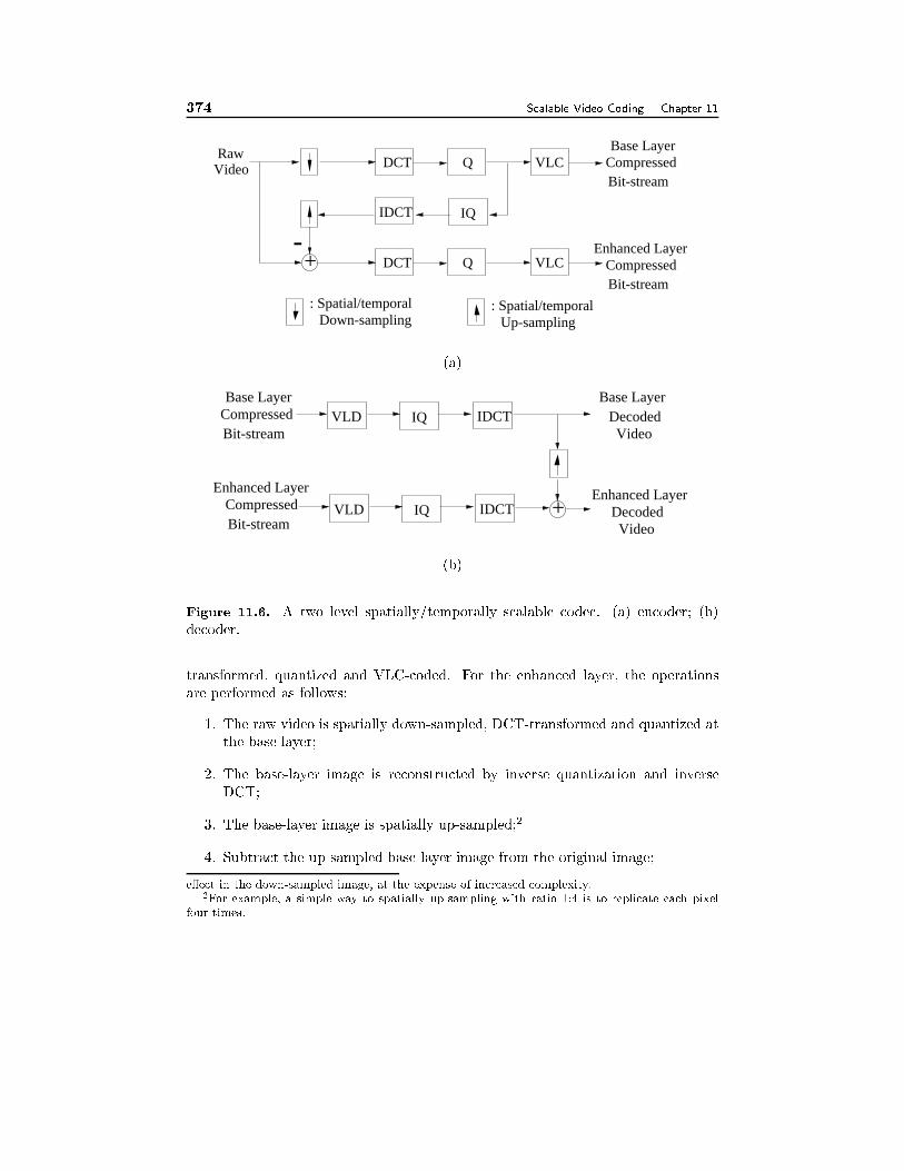
374 Scalable Video Coding Chapter 11
+
Base LayerCompressedBit-stream
IQ
VideoRaw
IDCT
-DCT Q
DCT Q VLC
VLC
Bit-streamCompressed
Enhanced Layer
: Spatial/temporal : Spatial/temporalDown-sampling Up-sampling
(a)
IDCT
IDCTVideo
VideoDecoded
+IQVLD
IQVLD
DecodedEnhanced Layer
Base Layer
Bit-streamCompressed
Bit-streamCompressedBase Layer
Enhanced Layer
(b)
Figure 11.6. A two level spatially/temporally scalable codec. (a) encoder; (b)
decoder.
transformed, quantized and VLC-coded. For the enhanced layer, the operations
are performed as follows:
1. The raw video is spatially down-sampled, DCT-transformed and quantized at
the base layer;
2. The base-layer image is reconstructed by inverse quantization and inverse
DCT;
3. The base-layer image is spatially up-sampled;2
4. Subtract the up-sampled base-layer image from the original image;
e�ect in the down-sampled image, at the expense of increased complexity.2For example, a simple way to spatially up-sampling with ratio 1:4 is to replicate each pixel
four times.
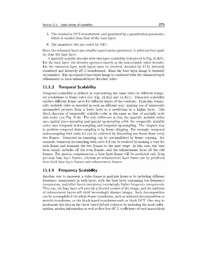
Section 11.1. Basic Modes of Scalability 375
5. The residual is DCT-transformed, and quantized by a quantization parameter,
which is smaller than that of the base layer;
6. The quantized bits are coded by VLC.
Since the enhanced layer uses smaller quantization parameter, it achieves �ner qual-
ity than the base layer.
A spatially scalable decoder with two-layer scalability is depicted in Fig. 11.6(b).
For the base layer, the decoder operates exactly as the non-scalable video decoder.
For the enhanced layer, both layers must be received, decoded by VLD, inversely
quantized and inversely DCT-transformed. Then the base-layer image is spatially
up-sampled. The up-sampled base-layer image is combined with the enhanced-layer
re�nements to form enhanced-layer decoded video.
11.1.3 Temporal Scalability
Temporal scalability is de�ned as representing the same video in di�erent tempo-
ral resolutions or frame rates (see Fig. 11.4(a) and 11.4(c)). Temporal scalability
enables di�erent frame rates for di�erent layers of the contents. Typically, tempo-
rally scalable video is encoded in such an eÆcient way: making use of temporally
up-sampled pictures from a lower layer as a prediction in a higher layer. The
block diagram of temporally scalable codec is the same as that of spatially scal-
able codec (see Fig. 11.6). The only di�erence is that the spatially scalable codec
uses spatial down-sampling and spatial up-sampling while the temporally scalable
codec uses temporal down-sampling and temporal up-sampling. The simplest way
to perform temporal down-sampling is by frame skipping. For example, temporal
down-sampling with ratio 2:1 can be achieved by discarding one frame from every
two frames. Temporal up-sampling can be accomplished by frame copying. For
example, temporal up-sampling with ratio 1:2 can be realized by making a copy for
each frame and transmit the two frames to the next stage. In this case, the base
layer simply includes all the even frames, and the enhancement layer all the odd
frames. For motion compensation, a base layer frame will be predicted only from
previous base layer frames, whereas an enhancement layer frame can be predicted
from both base layer frames and enhancement frames.
11.1.4 Frequency Scalability
Another way to represent a video frame in multiple layers is by including di�erent
frequency components in each layer, with the base layer containing low frequency
components, and other layers containing increasingly higher frequency components.
This way, the base layer will provide a blurred version of the image, and the addition
of enhancement layers will yield increasingly sharper images. Such decomposition
can be accomplished via whole-frame transforms, such as subband-decomposition or
wavelet transforms, or via block-based transforms such as block DCT. One way to
implement this idea in the block-based hybrid coders is by including the mode infor-
mation, motion information as well as �rst few DCT coeÆcients of each macroblock
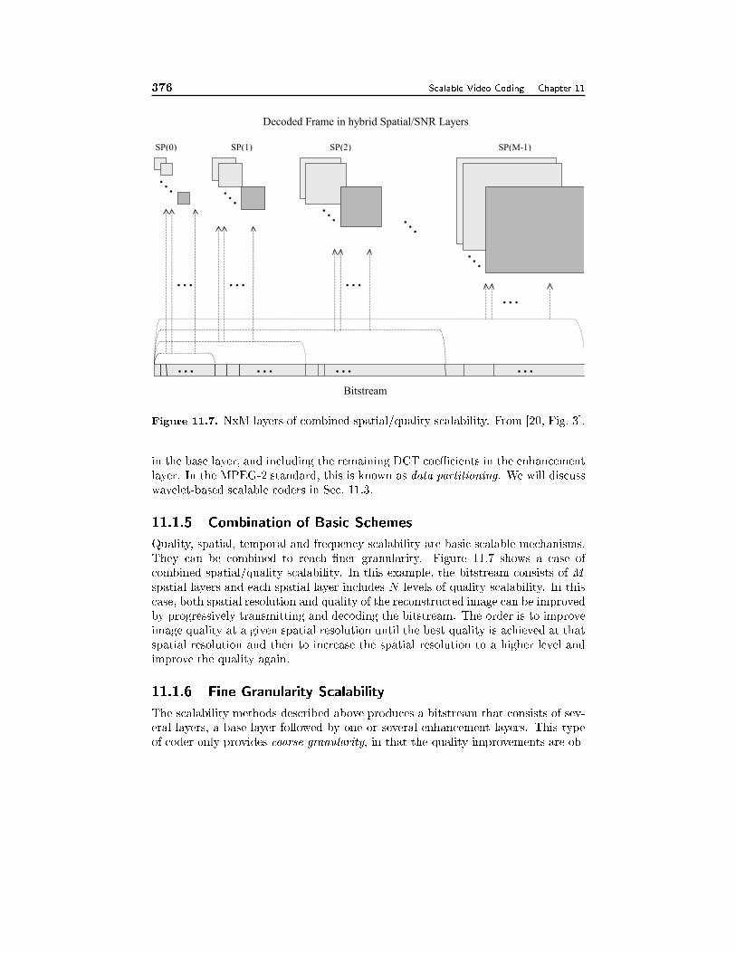
376 Scalable Video Coding Chapter 11
Decoded Frame in hybrid Spatial/SNR Layers
Bitstream
SP(0) SP(M-1)
SP(0)
SP(2)SP(1)
Figure 11.7. NxM layers of combined spatial/quality scalability. From [20, Fig. 3].
in the base layer, and including the remaining DCT coeÆcients in the enhancement
layer. In the MPEG-2 standard, this is known as data partitioning. We will discuss
wavelet-based scalable coders in Sec. 11.3.
11.1.5 Combination of Basic Schemes
Quality, spatial, temporal and frequency scalability are basic scalable mechanisms.
They can be combined to reach �ner granularity. Figure 11.7 shows a case of
combined spatial/quality scalability. In this example, the bitstream consists of M
spatial layers and each spatial layer includes N levels of quality scalability. In this
case, both spatial resolution and quality of the reconstructed image can be improved
by progressively transmitting and decoding the bitstream. The order is to improve
image quality at a given spatial resolution until the best quality is achieved at that
spatial resolution and then to increase the spatial resolution to a higher level and
improve the quality again.
11.1.6 Fine Granularity Scalability
The scalability methods described above produces a bitstream that consists of sev-
eral layers, a base layer followed by one or several enhancement layers. This type
of coder only provides coarse granularity, in that the quality improvements are ob-
Section 11.1. Basic Modes of Scalability 377
tained with rate increases in large discrete steps. If only a partial set of bits in a
particular layer is received, the reproduced video quality is determined to a large
extent by the received bits in the previous layers, not bene�ting from the bits re-
ceived from this layer. Fine granularity scalability (FGS) refers to a coding method
by which the rate as well as quality increment at a much smaller step. In the
limiting case when a bitstream can provide continuously improving video quality
with every additional bit, the underlying coding method is called embedded coding.
Obviously, FGS and embedded coding can adapt to bandwidth variations in real
networks more e�ectively.
In practice, the requirement that the bitstream be completely embedded or have
�ne granularity is often relaxed. A base layer may be �rst produced to provide a low
but guaranteed level of quality, and then an enhancement layer may be generated to
provide improvement in �ne granularity. This, e.g., is the method employed in the
FGS mode of MPEG-4 [14, 11]. In this method, the conventional block-based hybrid
coding method is employed to produce a base layer stream at a given frame rate,
using a relatively large QP. Then, for every coded frame (intra- or inter-coded), the
di�erences between the original DCT coeÆcients3 and the quantized ones in the
base layer (to be called re�nement coeÆcients) are coded into a �ne granularity
stream. This is accomplished by quantizing the re�nement coeÆcients using a very
small QP 4 and then representing the quantized indices through successive bit plane
encoding.
Speci�cally, the absolute values of quantized re�nement coeÆcients in each block
are speci�ed in binary representations. Starting from the highest bit plane that con-
tains non-zeros, each bit plane is successively coded using run-length coding block
by block. The runlengths can be coded using either Hu�man coding or arithmetic
coding. Typically, di�erent codebooks are used for di�erent bit planes because the
runlength distributions are di�erent across planes. When only a partial set of the
enhancement layer stream is decoded, depending on how many bit planes were in-
cluded in the retained bits, the reconstructed video will have a quality in between
that obtainable from the base layer only to that obtainable with the QP used on the
re�nement DCT coeÆcients. The granularity of the stream is at the bit plane level:
every additional complete bit plane will yield an improvement in the quantization
accuracy of the DCT coeÆcients by a factor of two.5
The above method only o�ers scalability in quality at a �xed spatial-temporal
resolution. To add temporal scalability, the base layer may include a sub-sampled
set of frames coded with a higher QP. For the enhancement layer, the remaining
frames are bidirectionally predicted from the base layer frames. The DCT coeÆ-
3For each block, the transform is applied to the original block or the motion compensation
error block, depending on whether the block is coded in the intra- or inter mode in the base layer.4No quanitization is performed if one wishes to obtain lossless representation at the highest
rate.5In fact, the granularity can be up to the codeword level for the run-length representation,
as every additional complete codeword received can improve the reconstruction accuracy of some
coeÆcients. Although, depending on the available bandwidth, it is more practical to truncate a
FGS stream at the bitplane level.
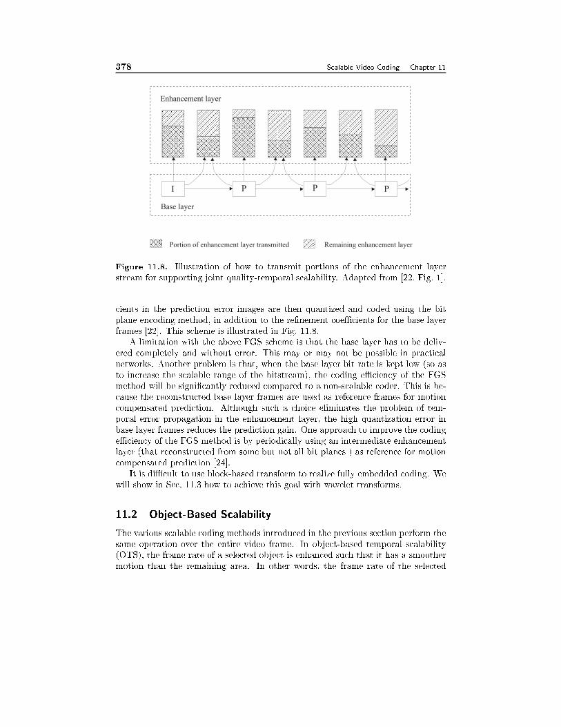
378 Scalable Video Coding Chapter 11
Enhancement layer
Base layer
I P P P
Portion of enhancement layer transmitted Remaining enhancement layer
Figure 11.8. Illustration of how to transmit portions of the enhancement layer
stream for supporting joint quality-temporal scalability. Adapted from [22, Fig. 1].
cients in the prediction error images are then quantized and coded using the bit
plane encoding method, in addition to the re�nement coeÆcients for the base layer
frames [22]. This scheme is illustrated in Fig. 11.8.
A limitation with the above FGS scheme is that the base layer has to be deliv-
ered completely and without error. This may or may not be possible in practical
networks. Another problem is that, when the base layer bit rate is kept low (so as
to increase the scalable range of the bitstream), the coding eÆciency of the FGS
method will be signi�cantly reduced compared to a non-scalable coder. This is be-
cause the reconstructed base layer frames are used as reference frames for motion
compensated prediction. Although such a choice eliminates the problem of tem-
poral error propagation in the enhancement layer, the high quantization error in
base layer frames reduces the prediction gain. One approach to improve the coding
eÆciency of the FGS method is by periodically using an intermediate enhancement
layer (that reconstructed from some but not all bit planes ) as reference for motion
compensated prediction [24].
It is diÆcult to use block-based transform to realize fully embedded coding. We
will show in Sec. 11.3 how to achieve this goal with wavelet transforms.
11.2 Object-Based Scalability
The various scalable coding methods introduced in the previous section perform the
same operation over the entire video frame. In object-based temporal scalability
(OTS), the frame rate of a selected object is enhanced such that it has a smoother
motion than the remaining area. In other words, the frame rate of the selected
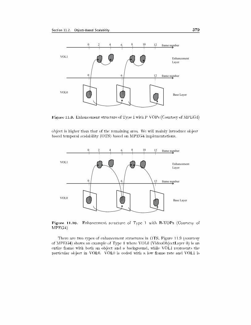
Section 11.2. Object-Based Scalability 379
VOL0
frame number
Base Layer
0 6 12
Enhancement
Layer
VOL1
frame number0 6 122 4 8 10
Figure 11.9. Enhancement structure of Type 1 with P-VOPs (Courtsey of MPEG4)
object is higher than that of the remaining area. We will mainly introduce object-
based temporal scalability (OTS) based on MPEG4 implementations.
VOL0
frame number
Base Layer
0 6 12
Enhancement
Layer
VOL1
frame number0 6 122 4 8 10
Figure 11.10. Enhancement structure of Type 1 with B-VOPs (Courtesy of
MPEG4)
There are two types of enhancement structures in OTS. Figure 11.9 (courtesy
of MPEG4) shows an example of Type 1 where VOL0 (VideoObjectLayer 0) is an
entire frame with both an object and a background, while VOL1 represents the
particular object in VOL0. VOL0 is coded with a low frame rate and VOL1 is
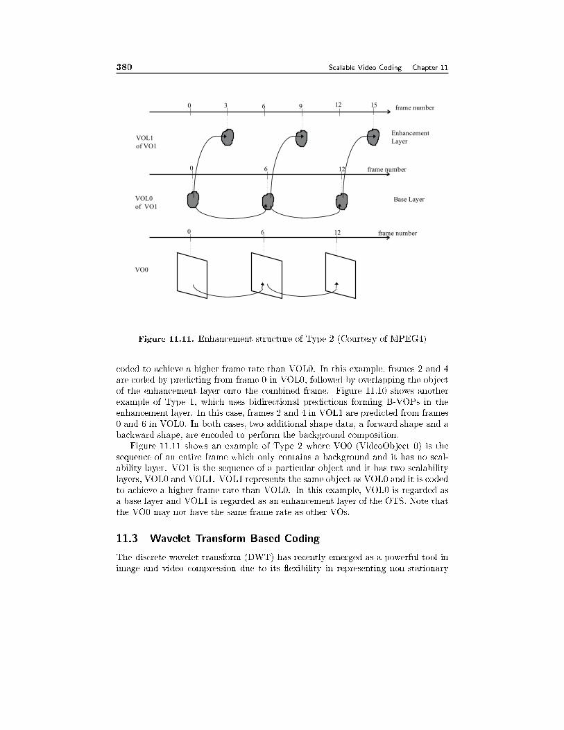
380 Scalable Video Coding Chapter 11
VO0
frame number0 6 12
VOL0
of VO1Base Layer
frame number0 6 12
Enhancement
LayerVOL1
of VO1
frame number0 6 123 9 15
Figure 11.11. Enhancement structure of Type 2 (Courtesy of MPEG4)
coded to achieve a higher frame rate than VOL0. In this example, frames 2 and 4
are coded by predicting from frame 0 in VOL0, followed by overlapping the object
of the enhancement layer onto the combined frame. Figure 11.10 shows another
example of Type 1, which uses bidirectional predictions forming B-VOPs in the
enhancement layer. In this case, frames 2 and 4 in VOL1 are predicted from frames
0 and 6 in VOL0. In both cases, two additional shape data, a forward shape and a
backward shape, are encoded to perform the background composition.
Figure 11.11 shows an example of Type 2 where VO0 (VideoObject 0) is the
sequence of an entire frame which only contains a background and it has no scal-
ability layer. VO1 is the sequence of a particular object and it has two scalability
layers, VOL0 and VOL1. VOL1 represents the same object as VOL0 and it is coded
to achieve a higher frame rate than VOL0. In this example, VOL0 is regarded as
a base layer and VOL1 is regarded as an enhancement layer of the OTS. Note that
the VO0 may not have the same frame rate as other VOs.
11.3 Wavelet Transform Based Coding
The discrete wavelet transform (DWT) has recently emerged as a powerful tool in
image and video compression due to its exibility in representing non-stationary
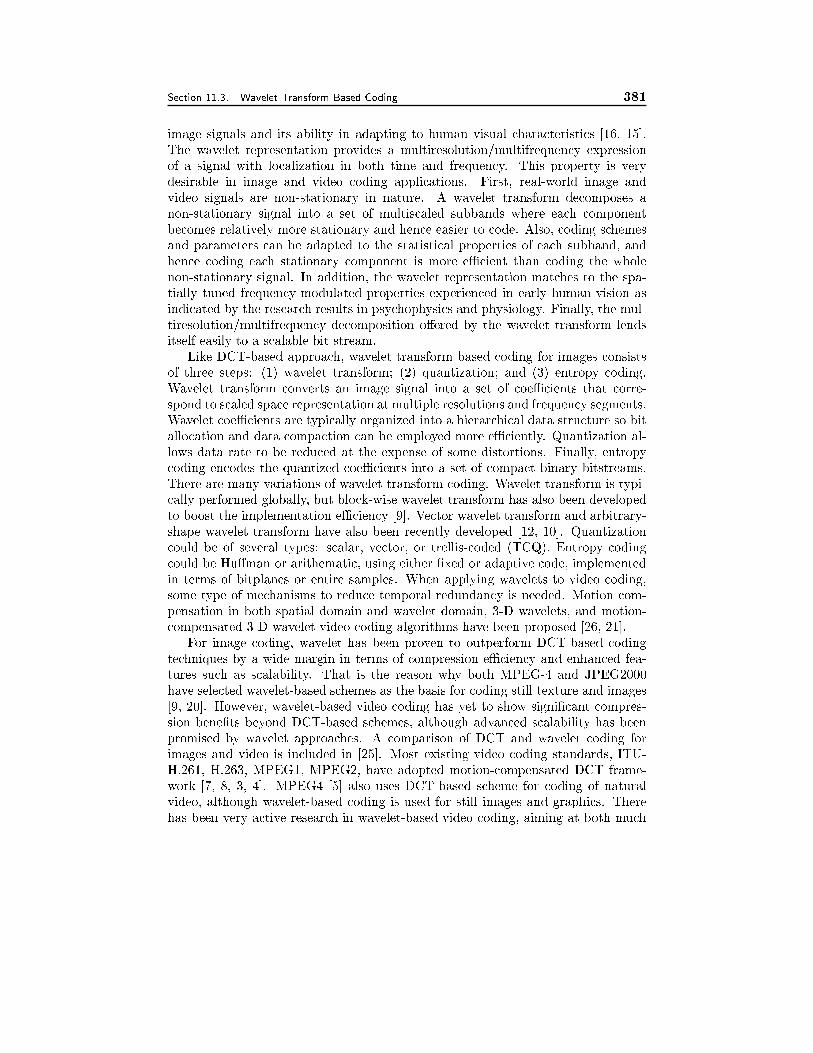
Section 11.3. Wavelet Transform Based Coding 381
image signals and its ability in adapting to human visual characteristics [16, 15].
The wavelet representation provides a multiresolution/multifrequency expression
of a signal with localization in both time and frequency. This property is very
desirable in image and video coding applications. First, real-world image and
video signals are non-stationary in nature. A wavelet transform decomposes a
non-stationary signal into a set of multiscaled subbands where each component
becomes relatively more stationary and hence easier to code. Also, coding schemes
and parameters can be adapted to the statistical properties of each subband, and
hence coding each stationary component is more eÆcient than coding the whole
non-stationary signal. In addition, the wavelet representation matches to the spa-
tially tuned frequency-modulated properties experienced in early human vision as
indicated by the research results in psychophysics and physiology. Finally, the mul-
tiresolution/multifrequency decomposition o�ered by the wavelet transform lends
itself easily to a scalable bit stream.
Like DCT-based approach, wavelet transform based coding for images consists
of three steps: (1) wavelet transform; (2) quantization; and (3) entropy coding.
Wavelet transform converts an image signal into a set of coeÆcients that corre-
spond to scaled space representation at multiple resolutions and frequency segments.
Wavelet coeÆcients are typically organized into a hierarchical data structure so bit
allocation and data compaction can be employed more eÆciently. Quantization al-
lows data rate to be reduced at the expense of some distortions. Finally, entropy
coding encodes the quantized coeÆcients into a set of compact binary bitstreams.
There are many variations of wavelet transform coding. Wavelet transform is typi-
cally performed globally, but block-wise wavelet transform has also been developed
to boost the implementation eÆciency [9]. Vector wavelet transform and arbitrary-
shape wavelet transform have also been recently developed [12, 10]. Quantization
could be of several types: scalar, vector, or trellis-coded (TCQ). Entropy coding
could be Hu�man or arithematic, using either �xed or adaptive code, implemented
in terms of bitplanes or entire samples. When applying wavelets to video coding,
some type of mechanisms to reduce temporal redundancy is needed. Motion com-
pensation in both spatial domain and wavelet domain, 3-D wavelets, and motion-
compensated 3-D wavelet video coding algorithms have been proposed [26, 21].
For image coding, wavelet has been proven to outperform DCT-based coding
techniques by a wide margin in terms of compression eÆciency and enhanced fea-
tures such as scalability. That is the reason why both MPEG-4 and JPEG2000
have selected wavelet-based schemes as the basis for coding still texture and images
[9, 20]. However, wavelet-based video coding has yet to show signi�cant compres-
sion bene�ts beyond DCT-based schemes, although advanced scalability has been
promised by wavelet approaches. A comparison of DCT and wavelet coding for
images and video is included in [25]. Most existing video coding standards, ITU-
H.261, H.263, MPEG1, MPEG2, have adopted motion-compensated DCT frame-
work [7, 8, 3, 4]. MPEG4 [5] also uses DCT-based scheme for coding of natural
video, although wavelet-based coding is used for still images and graphics. There
has been very active research in wavelet-based video coding, aiming at both much
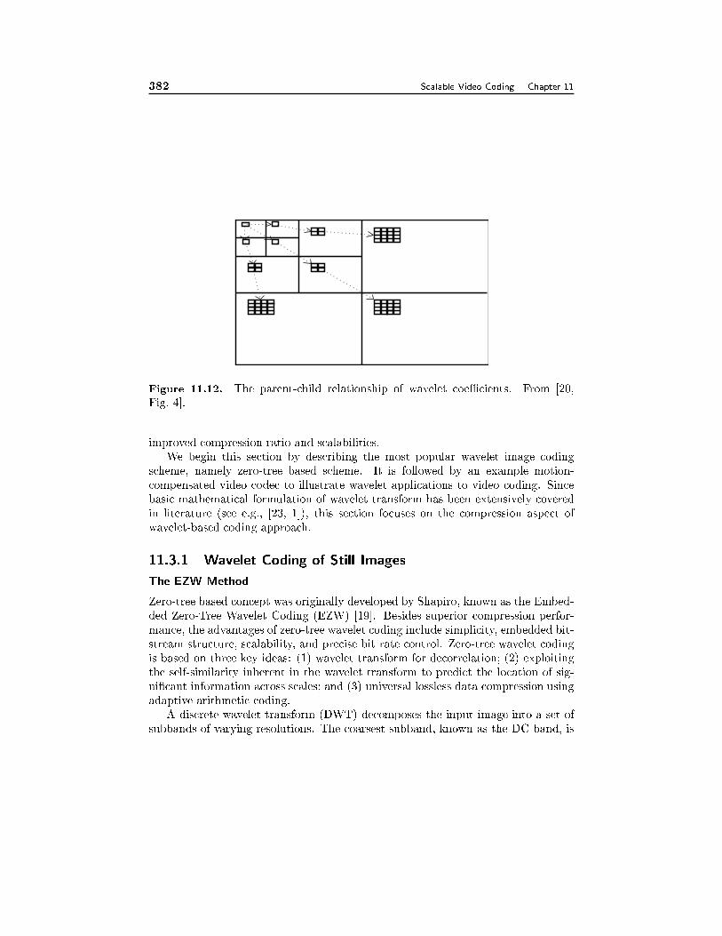
382 Scalable Video Coding Chapter 11
Figure 11.12. The parent-child relationship of wavelet coeÆcients. From [20,
Fig. 4].
improved compression ratio and scalabilities.
We begin this section by describing the most popular wavelet image coding
scheme, namely zero-tree based scheme. It is followed by an example motion-
compensated video codec to illustrate wavelet applications to video coding. Since
basic mathematical formulation of wavelet transform has been extensively covered
in literature (see e.g., [23, 1]), this section focuses on the compression aspect of
wavelet-based coding approach.
11.3.1 Wavelet Coding of Still Images
The EZW Method
Zero-tree based concept was originally developed by Shapiro, known as the Embed-
ded Zero-Tree Wavelet Coding (EZW) [19]. Besides superior compression perfor-
mance, the advantages of zero-tree wavelet coding include simplicity, embedded bit-
stream structure, scalability, and precise bit rate control. Zero-tree wavelet coding
is based on three key ideas: (1) wavelet transform for decorrelation; (2) exploiting
the self-similarity inherent in the wavelet transform to predict the location of sig-
ni�cant information across scales; and (3) universal lossless data compression using
adaptive arithmetic coding.
A discrete wavelet transform (DWT) decomposes the input image into a set of
subbands of varying resolutions. The coarsest subband, known as the DC band, is
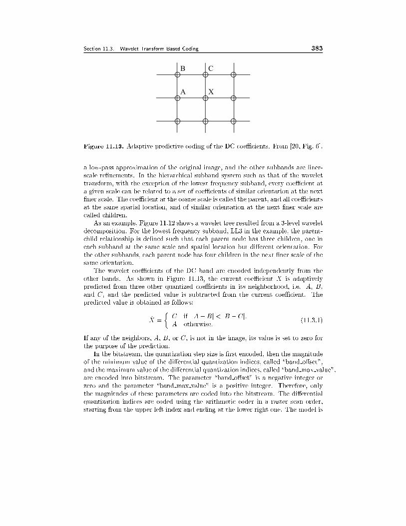
Section 11.3. Wavelet Transform Based Coding 383
B C
A X
Figure 11.13. Adaptive predictive coding of the DC coeÆcients. From [20, Fig. 6].
a low-pass approximation of the original image, and the other subbands are �ner-
scale re�nements. In the hierarchical subband system such as that of the wavelet
transform, with the exception of the lowest frequency subband, every coeÆcient at
a given scale can be related to a set of coeÆcients of similar orientation at the next
�ner scale. The coeÆcient at the coarse scale is called the parent, and all coeÆcients
at the same spatial location, and of similar orientation at the next �ner scale are
called children.
As an example, Figure 11.12 shows a wavelet tree resulted from a 3-level wavelet
decomposition. For the lowest frequency subband, LL3 in the example, the parent-
child relationship is de�ned such that each parent node has three children, one in
each subband at the same scale and spatial location but di�erent orientation. For
the other subbands, each parent node has four children in the next �ner scale of the
same orientation.
The wavelet coeÆcients of the DC band are encoded independently from the
other bands. As shown in Figure 11.13, the current coeÆcient X is adaptively
predicted from three other quantized coeÆcients in its neighborhood, i.e. A, B,
and C, and the predicted value is subtracted from the current coeÆcient. The
predicted value is obtained as follows:
X =
�C if jA�Bj < jB � Cj;
A otherwise:(11.3.1)
If any of the neighbors, A, B, or C, is not in the image, its value is set to zero for
the purpose of the prediction.
In the bitstream, the quantization step size is �rst encoded, then the magnitude
of the minimum value of the di�erential quantization indices, called \band o�set",
and the maximum value of the di�erential quantization indices, called \band max value",
are encoded into bitstream. The parameter \band o�set" is a negative integer or
zero and the parameter \band max value" is a positive integer. Therefore, only
the magnitudes of these parameters are coded into the bitstream. The di�erential
quantization indices are coded using the arithmetic coder in a raster scan order,
starting from the upper left index and ending at the lower right one. The model is
384 Scalable Video Coding Chapter 11
updated with each encoding of a bit of the predicted quantization index to adapt
to the statistics of the DC band.
EZW scans wavelet coeÆcients subband by subband. Parents are scanned before
any of their children. Each coeÆcient is compared against the current threshold T .
A coeÆcient is signi�cant if its amplitude is greater than T . Such a coeÆcient is then
encoded using one of the symbols, negative signi�cant (NS) or positive signi�cant
(PS). The zero-tree root (ZTR) symbol is used to signify a coeÆcient below T with
all its children also below T . The isolated zero (IZ) symbol signi�es a coeÆcient
below T but with at least one child not below T . For signi�cant coeÆcients, EZW
further encodes coeÆcient values using a successive approximation quantization
scheme. Coding is done by bit-planes, leading to an embedded stream.
The ZTE and MZTE Methods
EZW has been signi�cantly improved over the years. Examples include SPIHT [18],
predictive EZW [13], Zero-Tree Entropy Coding (ZTE) [17], and the more general
case Multi-scale ZTE [20]. Shape adaptive wavelet coding using zero-trees has also
been proposed for coding of objects with arbitrary shapes [10].
The Zero-Tree Entropy Coding (ZTE) [17] is based on, but di�ers signi�cantly
from, EZW coding. Similar to EZW, ZTE coding exploits the self-similarity in-
herent in the wavelet transform of images to predict the location of information
across wavelet scales. Although ZTE does not produce a fully embedded bitstream
as EZW, it gains exibility and other advantages over EZW coding, including sub-
stantial improvement in coding eÆciency, simplicity, and spatial scalability. ZTE
coding is performed by assigning a zero-tree symbol to a coeÆcient and then coding
the coeÆcient value with its symbol in one of the two di�erent scanning orders. The
four zero-tree symbols used in ZTE are zero-tree root (ZTR), valued zero-tree root
(VZTR), value (VAL), and isolated zero (IZ). The zero-tree symbols and quantized
coeÆcients are then losslessly encoded using an adaptive arithmetic coder with a
given symbol alphabet. The arithmetic encoder adaptively tracks the statistics of
the zero-tree symbols and encoded values using three models: 1) type to encode the
zero-tree symbols, 2) magnitude to encode the values in a bit-plane fashion, and
(3) sign to encode the sign of the value. For each coeÆcient its zero-tree symbol is
encoded �rst and if necessary, then its value is encoded. The value is encoded in
two steps. First, its absolute value is encoded in a bit-plane fashion using the ap-
propriate probability model and then the sign is encoded using a binary probability
model.
The Multi-scale Zero-Tree Entropy (MZTE) [20] coding technique is based on
ZTE coding but utilizes a new framework to improve and extend ZTE coding to a
fully scalable yet very eÆcient coding technique. At the �rst scalability layer, the
zero-tree symbols are generated in the same way as in ZTE coding and coded with
the non-zero wavelet coeÆcients of that scalability layer. For the next scalability
layer, the zero-tree map is updated along with the corresponding value re�nements.
In each scalability layer, a new zero-tree symbol is coded for a coeÆcient only if
Section 11.3. Wavelet Transform Based Coding 385
it was coded as ZTR or IZ in the previous scalability layer. If the coeÆcient is
coded as VZTR or VAL in the previous layer, only its re�nement value is coded in
the current layer. An additional probability model, residual, is used for encoding
the re�nements of the coeÆcients that are coded with a VAL or VZTR symbol in
any previous scalability layers. Furthermore, to utilize the highly correlated zero-
tree symbols between scalability layers, context modeling, based on the zero-tree
symbol of the coeÆcient in the previous scalability layer in MZTE, is used to better
estimate the distribution of zero-tree symbols.
The images in Figures 11.14(a) and 11.14(b) are obtained by JPEG and MZTE
compression schemes, respectively, at the same compression ratio of 45:1. The
results show that the MZTE scheme generates much better image quality with good
preservation of �ne texture regions and absence of the blocking e�ect, compared
with JPEG. The study in [25] showed that a wavelet-based coder can typically
outperform a DCT-based coder by about 1 dB in PSNR when the bitrate is the
same.
With the MZTE method, one can easily obtain spatial and quality scalabilities.
By decoding increasingly more bits from the bitstream of a MZTE compressed
image, one can obtain a bigger and and sharper renditions of the original image.
An example set of decoded images at di�erent bit rates has previously been shown
in Fig. 11.1.
Shape Adaptive MZTE
MZTE has also been extended to objects of arbitrary shapes [10]. In the shape
adaptive ZTE (SA-ZTE) method, the object shape mask is decomposed into a
pyramid of subbands so that we know which wavelet tree nodes have valid wavelet
coeÆcients and which ones have don't-care values. We have to pay attention to the
way of coding the multi-resolution arbitrarily shaped objects with these don't-care
values (corresponding to the out-of-boundary pixels or out-nodes). We discuss how
to extend the conventional zerotree coding method to the shape adaptive case.
As discussed in [10], the SA-ZTE decomposes the arbitrarily shaped objects in
the image domain to a hierarchical structure with a set of subbands of varying
resolutions. Each subband has a corresponding shape mask associated with it to
specify the locations of the valid coeÆcients in that subband. There are three types
of nodes in a tree: zeros, non-zeros, and out-nodes (with don't-care values). The
task is to extend the zero-tree coding method to the case with out-nodes. A simple
way is to set those don't-care values to zeros and then apply the zero-tree coding
method. However, this requires bits to code the out-notes such as a don't-care tree
(the parent and all of its children have don't-care values). This is a waste of bits
because out-nodes do not need to be coded as the shape mask already indicates
their status. Therefore, we should treat out-nodes di�erently from zeros. Although
we don't want to use bits to code an out-node, we have to decide what to do with
its children nodes. One way is not to code any information about the status of the
children nodes of the don't-care node. This way, we always assume that it has four
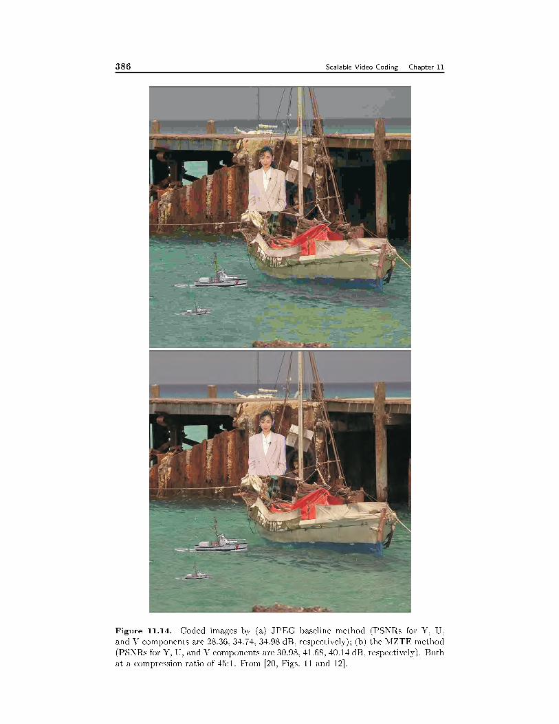
386 Scalable Video Coding Chapter 11
Figure 11.14. Coded images by (a) JPEG baseline method (PSNRs for Y, U,
and V components are 28.36, 34.74, 34.98 dB, respectively); (b) the MZTE method
(PSNRs for Y, U, and V components are 30.98, 41.68, 40.14 dB, respectively). Both
at a compression ratio of 45:1. From [20, Figs. 11 and 12].
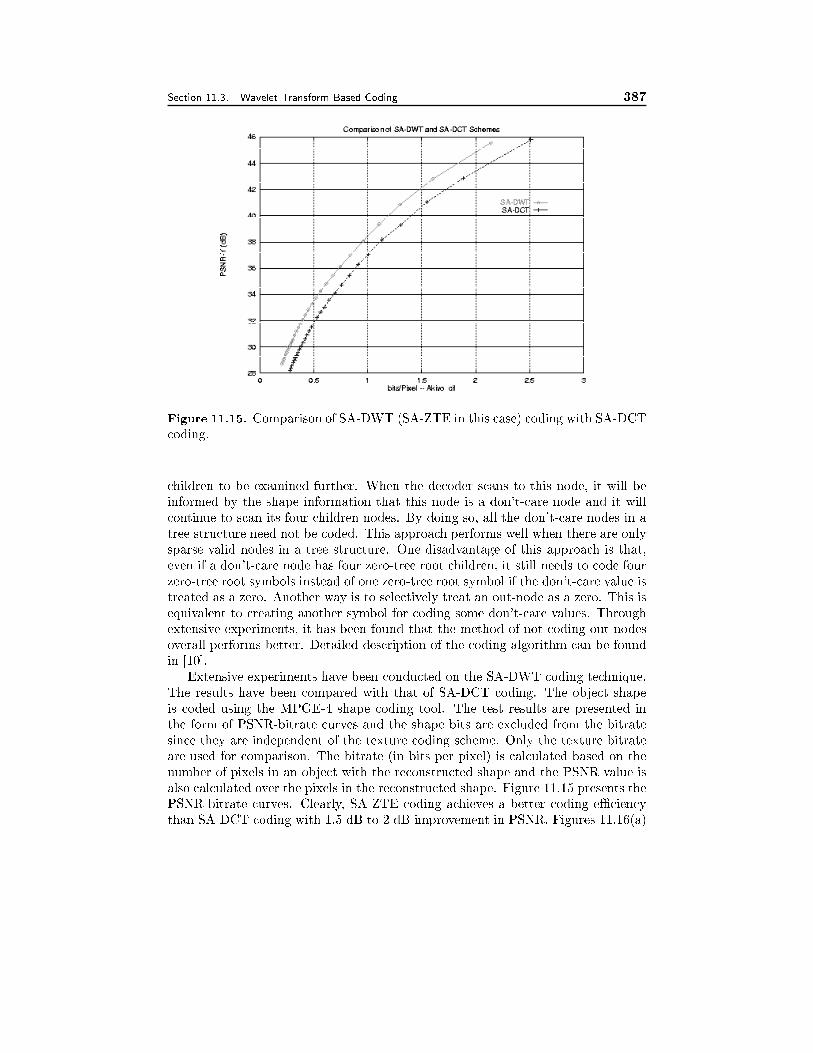
Section 11.3. Wavelet Transform Based Coding 387
Figure 11.15. Comparison of SA-DWT (SA-ZTE in this case) coding with SA-DCT
coding.
children to be examined further. When the decoder scans to this node, it will be
informed by the shape information that this node is a don't-care node and it will
continue to scan its four children nodes. By doing so, all the don't-care nodes in a
tree structure need not be coded. This approach performs well when there are only
sparse valid nodes in a tree structure. One disadvantage of this approach is that,
even if a don't-care node has four zero-tree root children, it still needs to code four
zero-tree root symbols instead of one zero-tree root symbol if the don't-care value is
treated as a zero. Another way is to selectively treat an out-node as a zero. This is
equivalent to creating another symbol for coding some don't-care values. Through
extensive experiments, it has been found that the method of not coding out-nodes
overall performs better. Detailed description of the coding algorithm can be found
in [10].
Extensive experiments have been conducted on the SA-DWT coding technique.
The results have been compared with that of SA-DCT coding. The object shape
is coded using the MPGE-4 shape coding tool. The test results are presented in
the form of PSNR-bitrate curves and the shape bits are excluded from the bitrate
since they are independent of the texture coding scheme. Only the texture bitrate
are used for comparison. The bitrate (in bits per pixel) is calculated based on the
number of pixels in an object with the reconstructed shape and the PSNR value is
also calculated over the pixels in the reconstructed shape. Figure 11.15 presents the
PSNR-bitrate curves. Clearly, SA-ZTE coding achieves a better coding eÆciency
than SA-DCT coding with 1.5 dB to 2 dB improvement in PSNR. Figures 11.16(a)
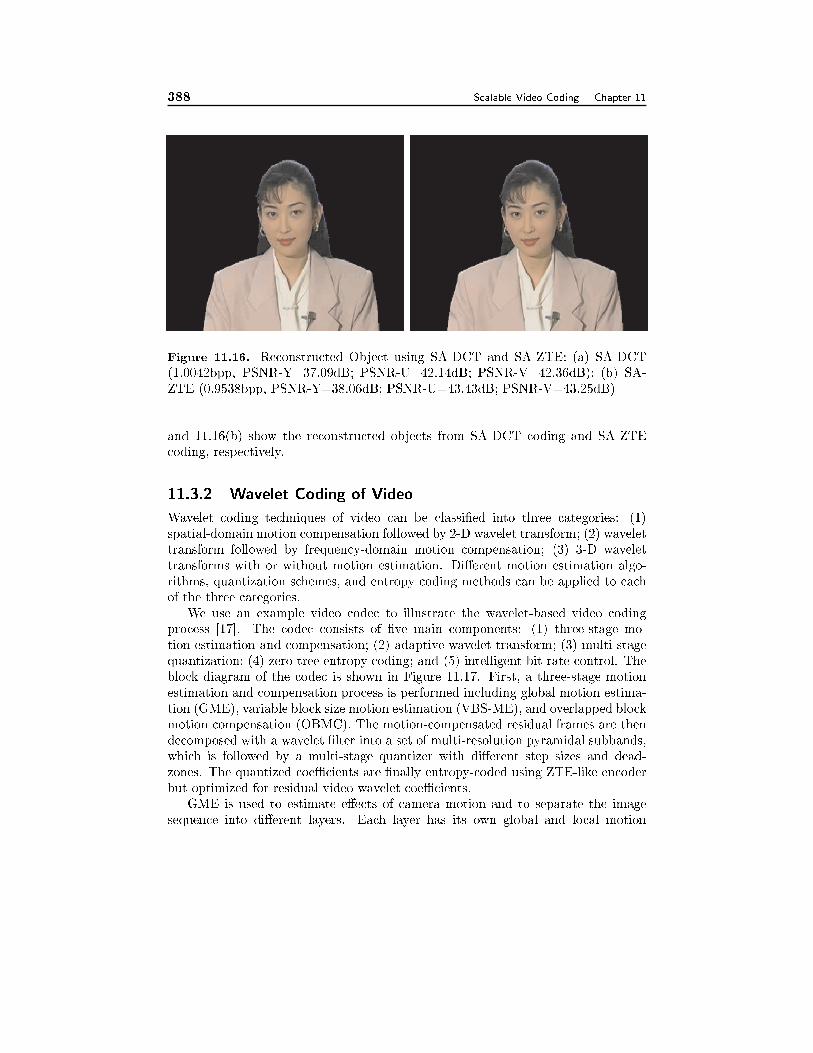
388 Scalable Video Coding Chapter 11
Figure 11.16. Reconstructed Object using SA-DCT and SA-ZTE: (a) SA-DCT
(1.0042bpp, PSNR-Y=37.09dB; PSNR-U=42.14dB; PSNR-V=42.36dB); (b) SA-
ZTE (0.9538bpp, PSNR-Y=38.06dB; PSNR-U=43.43dB; PSNR-V=43.25dB)
and 11.16(b) show the reconstructed objects from SA-DCT coding and SA-ZTE
coding, respectively.
11.3.2 Wavelet Coding of Video
Wavelet coding techniques of video can be classi�ed into three categories: (1)
spatial-domain motion compensation followed by 2-D wavelet transform; (2) wavelet
transform followed by frequency-domain motion compensation; (3) 3-D wavelet
transforms with or without motion estimation. Di�erent motion estimation algo-
rithms, quantization schemes, and entropy coding methods can be applied to each
of the three categories.
We use an example video codec to illustrate the wavelet-based video coding
process [17]. The codec consists of �ve main components: (1) three-stage mo-
tion estimation and compensation; (2) adaptive wavelet transform; (3) multi-stage
quantization; (4) zero-tree entropy coding; and (5) intelligent bit rate control. The
block diagram of the codec is shown in Figure 11.17. First, a three-stage motion
estimation and compensation process is performed including global motion estima-
tion (GME), variable block size motion estimation (VBS-ME), and overlapped block
motion compensation (OBMC). The motion-compensated residual frames are then
decomposed with a wavelet �lter into a set of multi-resolution pyramidal subbands,
which is followed by a multi-stage quantizer with di�erent step sizes and dead-
zones. The quantized coeÆcients are �nally entropy-coded using ZTE-like encoder
but optimized for residual video wavelet coeÆcients.
GME is used to estimate e�ects of camera motion and to separate the image
sequence into di�erent layers. Each layer has its own global and local motion
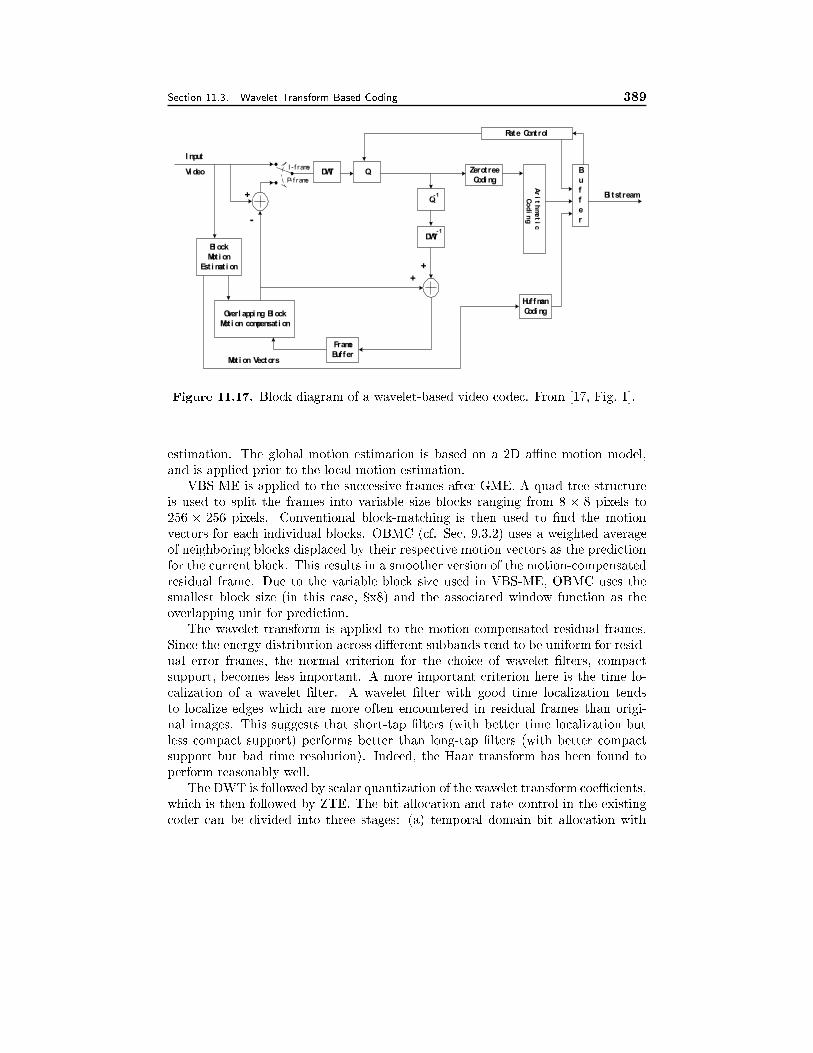
Section 11.3. Wavelet Transform Based Coding 389
Bl ock
Moti on
Esti mati on
Overl appi ng Bl ock
Moti on compensati on
Frame
Buffer
Huffman
Codi ng
DWT Q
Q
DWT
Zerotree
Codi ng
Ar
it
hm
et
ic
Co
di
ng
Rate Control
B
u
f
f
e
r
Bi tstream
+
+
+
-
Moti on Vectors
I nput
Vi deo
-1
-1
I - f rame
P-f rame
Figure 11.17. Block diagram of a wavelet-based video codec. From [17, Fig. 1].
estimation. The global motion estimation is based on a 2D aÆne motion model,
and is applied prior to the local motion estimation.
VBS-ME is applied to the successive frames after GME. A quad-tree structure
is used to split the frames into variable size blocks ranging from 8 � 8 pixels to
256 � 256 pixels. Conventional block-matching is then used to �nd the motion
vectors for each individual blocks. OBMC (cf. Sec. 9.3.2) uses a weighted average
of neighboring blocks displaced by their respective motion vectors as the prediction
for the current block. This results in a smoother version of the motion-compensated
residual frame. Due to the variable block size used in VBS-ME, OBMC uses the
smallest block size (in this case, 8x8) and the associated window function as the
overlapping unit for prediction.
The wavelet transform is applied to the motion-compensated residual frames.
Since the energy distribution across di�erent subbands tend to be uniform for resid-
ual error frames, the normal criterion for the choice of wavelet �lters, compact
support, becomes less important. A more important criterion here is the time lo-
calization of a wavelet �lter. A wavelet �lter with good time localization tends
to localize edges which are more often encountered in residual frames than origi-
nal images. This suggests that short-tap �lters (with better time localization but
less compact support) performs better than long-tap �lters (with better compact
support but bad time resolution). Indeed, the Haar transform has been found to
perform reasonably well.
The DWT is followed by scalar quantization of the wavelet transform coeÆcients,
which is then followed by ZTE. The bit allocation and rate control in the existing
coder can be divided into three stages: (a) temporal domain bit allocation with
390 Scalable Video Coding Chapter 11
variable frame rates; (b) inter-frame bit allocation to give optimal rate assignment
among frames; and (c) intra-frame bit allocation to produce optimal bit allocation
within a frame.
The above method has been compared to the MPEG-4's DCT-based coder [6].
The two methods produced similar performance in terms of PSNR [25]. It has
been found that optimization of quantization, entropy coding, and the complex
interplay among elements in the coding system is more important than optimizing
the transform itself.
11.4 Summary
� Scalability is a very useful feature since it allows exibility and adaptivity
to (1) changing network bandwidth; (2) varying channel conditions; and (3)
di�erent computing capabilities. Scalable coders are desirable for transport
over networks that have time varying bandwidth or error characteristics, or to
receivers that have varying access rates or processing capabilities. Scalability
is also desirable for video streaming applications, where the same video �le
may be accessed by users with di�erent communication links and computing
powers. Video streaming is discussed further in Chap. 15.
� Scalable coders can have either coarse granularity (two or three layers, also
called layered coders) or �ne granularity. In the extreme case of �ne granu-
larity, the bit stream is fully embedded and can be truncated at any point.
� Quality, spatial, temporal, and frequency scalability are basic scalable mech-
anisms. These schemes can be combined to achieve �ner granularity.
� One approach to obtain embedded streams at �xed spatial-temporal resolu-
tions is by successive bit plane encoding, as used both in �ne granularity
scalability mode of the MPEG-4 standard, and in most wavelet-based coders.
� Wavelet-based coders can be easily made to produce an embedded stream,
because the wavelet transform provides a multi-scale representation of the
signal.
11.5 Problems
11.1 What are the di�erences between layered and embedded coders? Give example
coders in each category.
11.2 Describe the four basic scalability modes: quality, spatial, temporal, fre-
quency.
11.3 How does the FGS method described in Sec. 11.1.6 work? What is the di�er-
ence between FGS and quality scalability?
Section 11.6. Bibliography 391
11.4 Consider i.i.d. Gaussian processes. Suppose that one can design a one layer
coder that reaches the distortion-rate bound, i.e., , the distortion and rate is
related by D = �2x2�2R, where �2
xis the source signal variance. Show that a
quality scalable coder with two quantization layers will reach the same D-R
bound, as the one-layer coder. Extend the proof to an arbitrary number of
layers. This means that for Gaussian processes, SNR scalability can achieve
the layered functionality without sacri�cing coding eÆciency. This result is
known as the successive re�nement property of the Gaussian process. To
explore further on this topic, see [2].
11.5 Starting from the program you created for the block-based hybrid video coder
for Prob. 9.15, generate a code for implementing two-layer quality scalability.
Compare the coding eÆciency of the original code and the layered coder for
a test sequence.
11.6 Starting from the program you created for the block-based hybrid video coder
for Prob. 9.15, generate a code for implementing two-layer spatial scalability.
Compare the coding eÆciency of the original code and the layered coder for
a test sequence.
11.7 What are the main di�erences between a block-wise transform such as the
DCT and the wavelet transform? What are the pros and cons of each?
11.8 How would you describe the EZW method to a friend who wants to know how
does it work?
11.9 Why is the wavelet transform more suitable for producing embedded streams?
How would you categorize the type of scalability that is o�ered by, say, the
EZW method? Does it o�er quality, spatial, and/or frequency scalability?
11.10 Implement the 2-stage wavelet transform for an image using the Haar wavelet
�lter. Examine the resulting image quality when coeÆcients in a chosen sub-
band are set to zero. Based on these images, comment on what type of features
does a particular band of wavelet coeÆcients reveal.
11.6 Bibliography
[1] A. Arkansu and R. A. Haddad. Multiresolution Signal Decomposition: Trans-
forms, Subbands, Wavelets. Academic Press, 1996.
[2] W. H. R. Equitz and T. M. Cover. Successive re�nement of information. IEEE
Trans. Inform. Theory, 37:269{275, Mar. 1991.
[3] ISO/IEC. IS 11172: Information technology { Coding of moving pictures and
associated audio for digital storage media at up to about 1.5 mbit/s, 1993. (MPEG-
1).
392 Scalable Video Coding Chapter 11
[4] ISO/IEC. IS 13818: Information technology { Generic coding of moving pictures
and associated audio information: Systems, 1995. (MPEG-2 Systems).
[5] ISO/IEC. IS 14496: Information technology { coding of audio-visual objects,
1999. (MPEG-4).
[6] ISO/IEC. Very low bitrate video codec. Public document, ISO/IEC
MPEG96/M0637, Munich, January 1996. (MPEG-4 VM).
[7] ITU-T. Recommendation H.261: Video codec for audiovisual services at px64
kbits, 1993.
[8] ITU-T. Recommendation H.263: Video coding for low bit rate communication,
1998.
[9] ISO/IEC JTC1/SC29/WG1. FCD 15444-1: Information technology - JPEG2000
image coding system, March 2000. available at http://www.jpeg.org/FCD15444-
1.htm.
[10] S. Li and W. Li. Shape-adaptive discrete wavelet transforms for arbitrarily
shaped visual object coding. IEEE Trans. Circuits Syst. for Video Technology,
10:725{743, Aug. 2000.
[11] W. Li. Fine granularity scalability in MPEG-4 for streaming video. In Proc.
IEEE Int. Conf. Circuits and Systems, Geneva, Switzerland, May 2000.
[12] W. Li and Y.-Q.Zhang. Vector-based signal processing and quantization for
image and video compression. Proceedings of IEEE, pages 671{691, Feb. 1995.
[13] J. Liang. Highly scalable image coding for multimedia applications. In ACM
Multimedia, Seattle, WA, October 1997.
[14] F. Ling, W. Li, and H. Q. Sun. Bitplane coding of DCT coeÆcients for image
and video compression. In Proc. SPIE Conf. Visual Commun. Image Processing,
San Jose, USA, Jan. 1999.
[15] S. Mallat. Multifrequency channel decompositions of images and wavelet mod-
els. IEEE Trans. Acoust., Speech, Signal Processing, 17, Dec. 1989.
[16] S. Mallat. A theory of multiresolution signal decomposition: The wavelet
representation. IEEE Trans. on Pattern Analysis and Machine Intell., 11:674{
693, 1989.
[17] S. A. Martucci, I. Sodagar, T. Chiang, and Y.-Q. Zhang. A zerotree wavelet
video coder. IEEE Trans. Circuits Syst. for Video Technology, 7(1):109{118, Feb.
1997.
[18] A. Said and W. Pearlman. A new, fast, and eÆcient image codec based on set
partitioning in hierarchical trees. IEEE Trans. Circuits Syst. for Video Technology,
6:243{250, June 1996.
Section 11.6. Bibliography 393
[19] J. M. Shapiro. Embedded image coding using zerotrees of wavelet coeÆcients.
IEEE Trans. Signal Processing, 41:3445{3462, Dec. 1993.
[20] I. Sodagar, H.-J. Lee, P.Hatrack, and Y.-Q.Zhang. Scalable wavelet coding for
synthetic/natural hybrid images. IEEE Trans. Circuits Syst. for Video Technology,
9:244{254, March 1999.
[21] D. Taubman and A. Zakhor. Multirate 3-D subband coding of video. IEEE
Trans. Image Process., 3:572{588, Sept. 1994.
[22] M. van der Schaar and H. Radha. A novel MPEG-4 based hybrid temporal-
snr scalability for internet video. In Proc. IEEE Int. Conf. Image Processing,
Vancouver, Canada, Sept. 2000.
[23] M. Vetterli and J. Kovacevic. Wavelets and Subband Coding. Prentice Hall,
New Jersey, 1995.
[24] F. Wu, S. Li, and Y.-Q. Zhang. DCT-prediction based progressive �ne gran-
ularity scalable coding. In Proc. IEEE Int. Conf. Image Processing, Vancouver,
CANADA, Sept. 2000.
[25] Z. Xiong, K. Ramachandran, M. Orchard, and Y.-Q. Zhang. A comparative
study of DCT- and wavelet-based image coding. IEEE Trans. Circuits Syst. for
Video Technology, 9(5):692{695, Aug. 1999.
[26] Y.-Q. Zhang and S. Zafar. Motion-compensated wavelet transform coding
for color video compression. IEEE Trans. Circuits Syst. for Video Technology,
2(3):285{296, Sept. 1992.
Chapter 12
STEREO AND MULTIVIEW
SEQUENCE PROCESSING
Acquisition and display of stereoscopic and more generally multiview sequences havemany applications. In industries, stereo display is used for object handling andinspection by robots in environment under hazard conditions. For medical applica-tions, stereoscopic probes are providing more useful information than a monoscopicone. For scienti�c exploration and visualization, stereoscopic or multiview displayenables the human being to experience 3-D environment over a at 2-D screen.Such applications have long existed, where stereo sequences have traditionally be-ing acquired, stored, and displayed in an analog format. A recent boost for 3-Dvision however comes from the advancement of digital television technology. Asdigital TV including HDTV becomes a reality, digital 3DTV is foreseen to be thenext quantum leap for the television industry, promising to o�er 3-D perception,in addition to sharper images. Another more recent application for stereo/3-D dis-play lies in virtual reality and human-computer interface, where 3-D rendering anddisplay gives viewers an illusion of physically interacting with people or objects ina remote (or non-existent) site.
In this chapter, we start with a brief discussion of the mechanism for perceivingdepth in the human visual system (Sec. 12.1). We then move on to the technicalaspects of stereo imaging and show how the 3-D position of an imaged point isrelated to its projections in a stereo image pair (Sec. 12.2). Next we discuss thetechnically most challenging problem in stereo sequence processing: disparity andconsequently depth from stereo (Sec. 12.3). Finally, we present approaches forcoding of stereoscopic and multiview video (Sec. 12.5). These topics are chosenbecause they belong to signal processing aspects of stereo and multiview systems.For coverage of stereo and multiview capture and display systems, see e.g., [16].
12.1 Depth Perception Through Stereopsis
Stereoscopic imaging and display is motivated by how humans perceive depth:through two separate eyes. Although there are several monocular cues that the
394
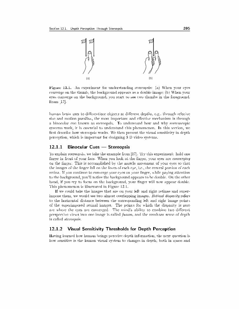
Section 12.1. Depth Perception Through Stereopsis 395
(a) (b)
Figure 12.1. An experiment for understanding stereopsis: (a) When your eyesconverge on the thumb, the background appears as a double image; (b) When youreyes converge on the background, you start to see two thumbs in the foreground.From [17].
human brain uses to di�erentiate objects at di�erent depths, e.g., through relativesize and motion parallax, the most important and e�ective mechanism is througha binocolar cue known as stereopsis. To understand how and why stereoscopicsystems work, it is essential to understand this phenomenon. In this section, we�rst describe how stereopsis works. We then present the visual sensitivity in depthperception, which is important for designing 3-D video systems.
12.1.1 Binocular Cues | Stereopsis
To explain stereopsis, we take the example from [17]. Try this experiment: hold one�nger in front of your face. When you look at the �nger, your eyes are convergingon the �nger. This is accomplished by the muscle movement of your eyes so thatthe images of the �nger fall on the fovea of each eye, i.e., the central portion of eachretina. If you continue to converge your eyes on your �nger, while paying attentionto the background, you'll notice the background appears to be double. On the otherhand, if you try to focus on the background, your �nger will now appear double.This phenomenon is illustrated in Figure 12.1.
If we could take the images that are on your left and right retinae and super-impose them, we would see two almost overlapping images. Retinal disparity refersto the horizontal distance between the corresponding left and right image pointsof the superimposed retinal images. The points for which the disparity is zeroare where the eyes are converged. The mind's ability to combine two di�erentperspective views into one image is called fusion, and the resultant sense of depthis called stereopsis.
12.1.2 Visual Sensitivity Thresholds for Depth Perception
Having learned how human beings perceive depth information, the next question ishow sensitive is the human visual system to changes in depth, both in space and
396 Stereo and Multiview Sequence Processing Chapter 12
time. In Chapter 2.4, we discussed visual thresholds in detecting spatial (in thesame 2-D plane) and temporal changes in monoscopic images. We learned that thecontrast sensitivity as a function of spatial frequency exhibits a band-pass charac-teristics at low temporal frequencies (maximum sensitivity at approximately 4 cpd)and a low-pass characteristics at high temporal frequencies. Similarly, the visualsensitivity with respect to temporal changes is band-pass at low spatial frequencies(maximum sensitivity at approximately 8-15 Hz), and is low-pass at high spatialfrequencies. These �ndings have guided the design of video display systems. Inorder to portray as much as the eye can see, a display should be able to producea spatial frequency of at least 64 cpd (the resolution in terms of pixels depends onthe picture height and width and the viewing distance) and a temporal frequencyof 70 Hz.
To design a 3-D video capture and display system, an important issue is thevisual threshold in depth perception. Because the depth is perceived through retinaldisparities, visual sensitivity to depth can be evaluated in terms of the variation indisparity. Results quoted below are from Pastoor [11].
Sensitivity to depth variation in space and time It has been found that thevisual sensitivity for spatial and temporal changes of the disparity lies signi�cantlybelow the sensitivity for image contrast variations. Thus, a display system thatmeets the spatial and temporal bandwidth requirement of the contrast sensitivityfunction would also enable satisfactory perception of depth variation, both spatiallyand temporally. It has been found that the visual sensitivity in terms of the spatialfrequency of the disparity �eld has a band-pass characteristic with a bandwidth of3{4 cpd. The maximum sensitivity lies in the range of 0.2{0.5 cpd. The upper limitfor temporal changes in disparity which are still perceptible as movements in depthlies in the region of 4{6 Hz.
Sensitivity to disparity quantization It has been found that the threshold ofstereoscopic acuity, that is, the ability to resolve stimuli in depth, is about 2 secondsof arc.1 Such �ne di�erences in depth can be perceived if the horizontal image res-olution for both left and right images are at least 24 cpd. With digital display, theprojected disparity and consequently the apparent depth is quantized. When thequantization is too coarse, the objects in the scene may appear to belong to layersof at scenery at di�erent depths and object motion in depth may also appear jerky.
Sensitivity to view angle quantization In natural vision, when a viewer moves,his/her viewpoint moves continuously. With 3-D display systems o�ering multipleviewpoints, only a limited number of viewpoints can be realized, which can bethought of as quantizing the direction of the viewing angle. Such quantization hasthe e�ect that, when the observer changes his/her position in front of the display,sudden shifts take place between perceived views. It has been demonstrated thatview angle shifts must lie within a threshold of approximately 1 min of arc for thesubjective quality to be rated \good" on the CCIR quality assessment scale.
11 second of arc is 1/3600 of a degree.
Section 12.2. Stereo Imaging Principle 397
Asymmetric spatial resolution requirement Various experiments have shown thatin stereo display, the resolution of one image can be considerably reduced (up tohalf) without causing deterioration in the subjective impression of sharpness, whenthe other image is displayed with suÆcient resolution as dictated by the visualspatial-temporal thresholds, at least for a short period. It is not known to whatdegree such a display leads to visual strain when viewed over a long period of time.This asymmetrical property has been explored in stereo sequence compression (seeSec. 12.5.3). By reducing the sampling resolution of one view by half in bothhorizontal and vertical directions, a compression factor of four can be achievedimmediately.
Asynchronous fusion of binocular views Within certain limits of disparity values,the visual system is capable of fusing the two images of a stereo pair presentedasynchronously as long as the delay between the presentations does not exceed 50ms [14]. This fact has been taken advantage in �eld sequential display systems. Thedelay between the left and right views can lead to distortions of depth when theobjects being displayed move. It has been found that a delay of 160 ms can createvisible depth distortion.
12.2 Stereo Imaging Principle
Stereoscopic imaging and display systems are designed to emulate human stereoperception: capturing a 3-D scene using two cameras located in slightly shiftedpositions, and then presenting the two images separately to each eye. In this section,we describe the principle of stereoscopic imaging and show how to deduce the depthof a 3-D point from its image positions in two di�erent imaging planes. We will seethat, in fact, to capture the depth information, the two cameras do not have to beparallel as our human eyes, although such an arrangement leads to mathematicallysimple relationships between depth and image correspondence. We will start byconsidering a system with two cameras in arbitrary positions. We will then focuson two special cases: one with two cameras sharing the same imaging plane, anotherwith two cameras oriented towards each other.
12.2.1 Arbitrary Camera
We start by considering two arbitrarily positioned cameras. Consider an arbitrarycamera con�guration shown in Fig. 12.2. Let [R]l and tl (resp. [R]r and tr) denotethe rotation matrix and the translation vector required to align the left (resp. right)camera coordinate (Cl and Cr) with a chosen world coordinate (Cw). Then thecoordinates of the left and right cameras, Xl = [Xl; Yl; Zl]
T and Xr = [Xr; Yr; Zr]T ,
are related to the world coordinate X = [X;Y; Z]T by
Xl = [R]lX+ tl; Xr = [R]rX+ tr: (12.2.1)
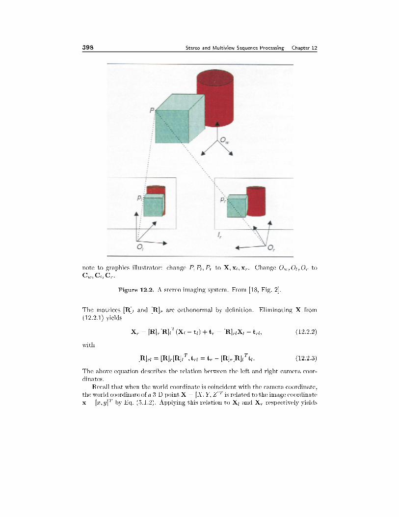
398 Stereo and Multiview Sequence Processing Chapter 12
note to graphics illustrator: change P; Pl; Pr to X;xl;xr. Change Ow; Ol; Or toCw;Cl;Cr:
Figure 12.2. A stereo imaging system. From [18, Fig. 2].
The matrices [R]l and [R]r are orthonormal by de�nition. Eliminating X from(12.2.1) yields
Xr = [R]r[R]lT(Xl � tl) + tr = [R]rlXl + trl; (12.2.2)
with
[R]rl = [R]r[R]lT; trl = tr � [R]r[R]l
Ttl: (12.2.3)
The above equation describes the relation between the left and right camera coor-dinates.
Recall that when the world coordinate is coincident with the camera coordinate,the world coordinate of a 3-D pointX = [X;Y; Z]T is related to the image coordinatex = [x; y]T by Eq. (5.1.2). Applying this relation to Xl and Xr respectively yields
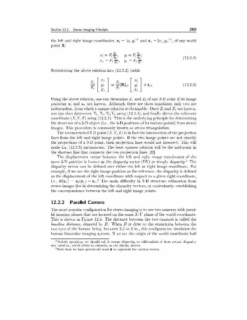
Section 12.2. Stereo Imaging Principle 399
the left and right image coordinates, xl = [xl; yl]T and xr = [xr; yr]
T , of any worldpoint X:
xl = FlXl
Zl
; yl = FlYlZl
;
xr = FrXr
Zr
; yr = FrYrZr
:(12.2.4)
Substituting the above relation into (12.2.2) yields
Zr
Fr
24 xryrFr
35 =
Zl
Fl[R]rl
24 xlylFl
35+ trl: (12.2.5)
Using the above relation, one can determine Zr and Zl of any 3-D point if its imagepositions xl and xr are known. Although there are three equations, only two areindependent, from which a unique solution is obtainable. Once Zl and Zr are known,one can then determine Xl; Xr; Yl; Yr using (12.2.4), and �nally derive the referencecoordinate (X;Y; Z) using (12.2.1). This is the underlying principle for determiningthe structure of a 3-D object (i.e., the 3-D positions of its various points) from stereoimages. This procedure is commonly known as stereo triangulation.
The reconstructed 3-D point (X;Y; Z) is in fact the intersection of the projectionlines from the left and right image points. If the two image points are not exactlythe projections of a 3-D point, their projection lines would not intersect. This willmake Eq. (12.2.5) inconsistent. The least squares solution will be the mid-point inthe shortest line that connects the two projection lines [22].
The displacement vector between the left and right image coordinates of thesame 3-D position is known as the disparity vector (DV) or simply disparity.
2 Thedisparity vector can be de�ned over either the left or right image coordinate. Forexample, if we use the right image position as the reference, the disparity is de�nedas the displacement of the left coordinate with respect to a given right coordinate,i.e., d(xr) = xl(xr) � xr:
3 The main diÆculty in 3-D structure estimation fromstereo images lies in determining the disparity vectors, or equivalently, establishingthe correspondence between the left and right image points.
12.2.2 Parallel Camera
The most popular con�guration for stereo imaging is to use two cameras with paral-lel imaging planes that are located on the same X-Y plane of the world coordinate.This is shown in Figure 12.3. The distance between the two cameras is called thebaseline distance, denoted by B. When B is close to the separation between thetwo eyes of the human being, between 2.5 to 3 in., this con�guration simulates thehuman binocular imaging system. If we set the origin of the world coordinate half
2Strictly speaking, we should call it image disparity, to di�erentiate it from retinal disparity
and parallax, which refers to disparity at the display screen.3Note that we have previously used d to represent the motion vector.
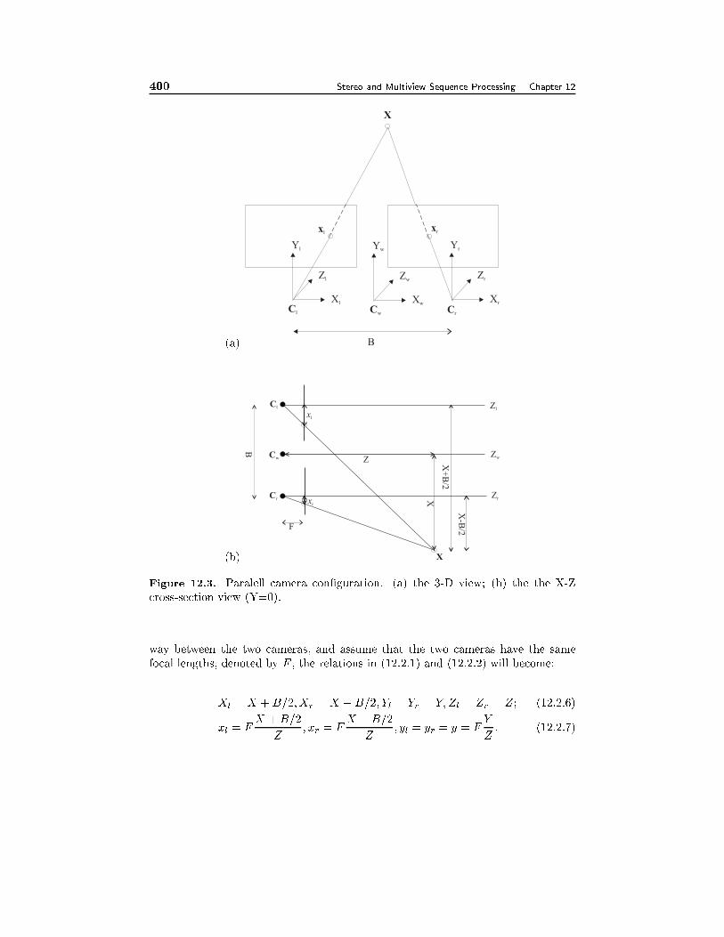
400 Stereo and Multiview Sequence Processing Chapter 12
(a)
Cl
xl
Cr
xr
Xl Xr
X
Yl Yr
Zl
Cw
Xw
Yw
ZwZr
B
(b)
X+
B/2
X
X-B
/2
Z
Zl
Zw
Zr
B
F
xl
xr
Cl
Cr
X
Cw
Figure 12.3. Paralell camera con�guration. (a) the 3-D view; (b) the the X-Zcross-section view (Y=0).
way between the two cameras, and assume that the two cameras have the samefocal lengths, denoted by F , the relations in (12.2.1) and (12.2.2) will become:
Xl = X +B=2; Xr = X �B=2; Yl = Yr = Y; Zl = Zr = Z; (12.2.6)
xl = FX +B=2
Z; xr = F
X �B=2
Z; yl = yr = y = F
Y
Z: (12.2.7)
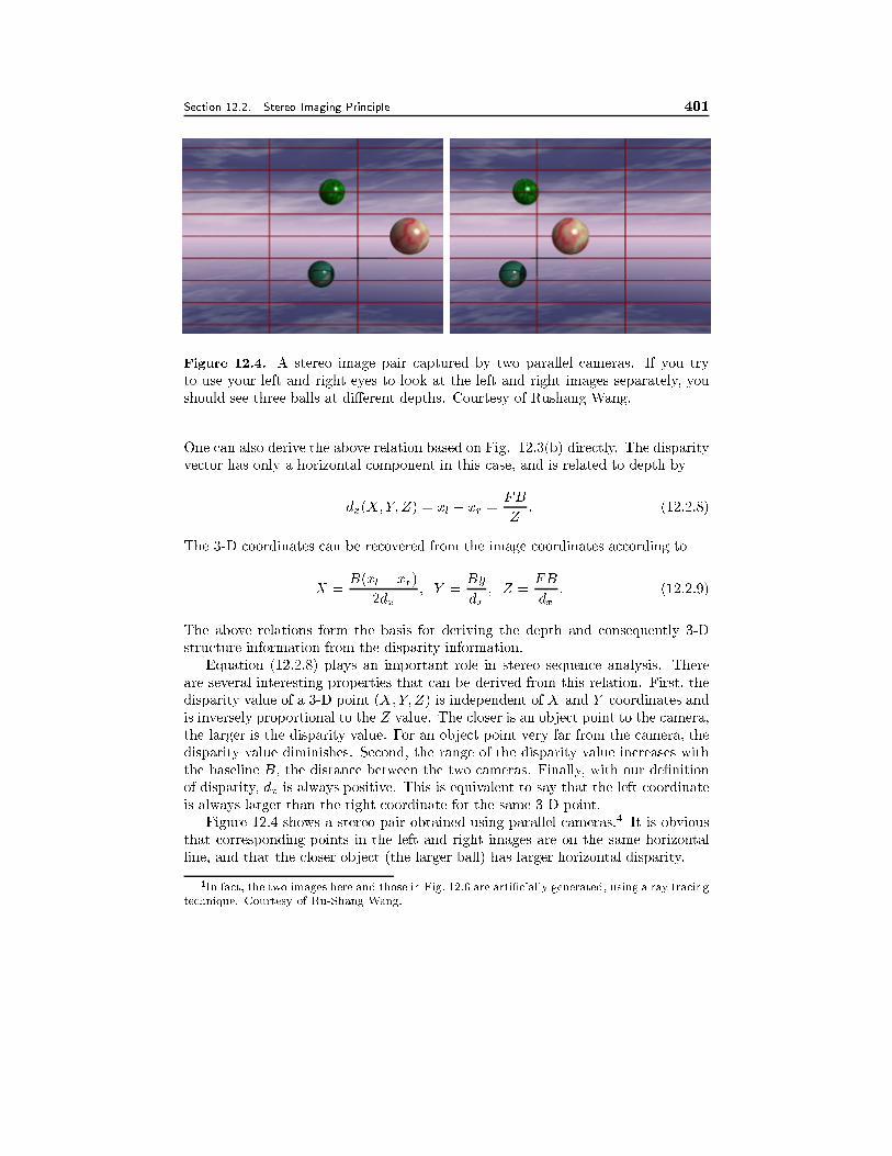
Section 12.2. Stereo Imaging Principle 401
Figure 12.4. A stereo image pair captured by two parallel cameras. If you tryto use your left and right eyes to look at the left and right images separately, youshould see three balls at di�erent depths. Courtesy of Rushang Wang.
One can also derive the above relation based on Fig. 12.3(b) directly. The disparityvector has only a horizontal component in this case, and is related to depth by
dx(X;Y; Z) = xl � xr =FB
Z: (12.2.8)
The 3-D coordinates can be recovered from the image coordinates according to
X =B(xl + xr)
2dx; Y =
By
dx; Z =
FB
dx: (12.2.9)
The above relations form the basis for deriving the depth and consequently 3-Dstructure information from the disparity information.
Equation (12.2.8) plays an important role in stereo sequence analysis. Thereare several interesting properties that can be derived from this relation. First, thedisparity value of a 3-D point (X;Y; Z) is independent of X and Y coordinates andis inversely proportional to the Z value. The closer is an object point to the camera,the larger is the disparity value. For an object point very far from the camera, thedisparity value diminishes. Second, the range of the disparity value increases withthe baseline B, the distance between the two cameras. Finally, with our de�nitionof disparity, dx is always positive. This is equivalent to say that the left coordinateis always larger than the right coordinate for the same 3-D point.
Figure 12.4 shows a stereo pair obtained using parallel cameras.4 It is obviousthat corresponding points in the left and right images are on the same horizontalline, and that the closer object (the larger ball) has larger horizontal disparity.
4In fact, the two images here and those in Fig. 12.6 are arti�cially generated, using a ray tracing
technique. Courtesy of Ru-Shang Wang.
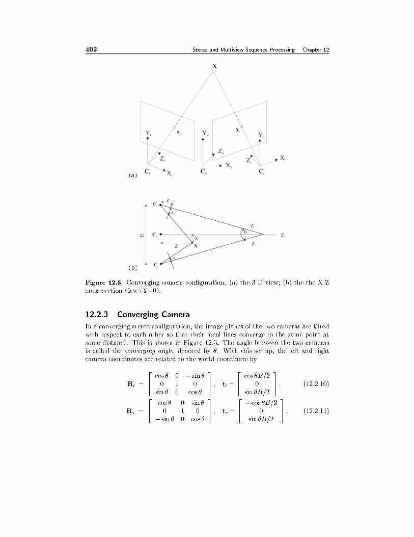
402 Stereo and Multiview Sequence Processing Chapter 12
(a)Cl Cr
Zl
Yl
XrZr
Yr
xlxr
X
XlCw
Xw
Yw
Zw
(b)
�
Cl
xl
xr
Cr
B
X
Z
F
Cw
Zr
Zl
Zw
X
Figure 12.5. Converging camera con�guration. (a) the 3-D view; (b) the the X-Zcross-section view (Y=0).
12.2.3 Converging Camera
In a converging stereo con�guration, the image planes of the two cameras are tiltedwith respect to each other so that their focal lines converge to the same point atsome distance. This is shown in Figure 12.5. The angle between the two camerasis called the converging angle, denoted by �. With this set-up, the left and rightcamera coordinates are related to the world coordinate by
Rl =
24 cos � 0 � sin �
0 1 0sin � 0 cos �
35 ; tl =
24 cos �B=2
0sin �B=2
35 ; (12.2.10)
Rr =
24 cos � 0 sin �
0 1 0� sin � 0 cos �
35 ; tr =
24 � cos �B=2
0sin �B=2
35 : (12.2.11)
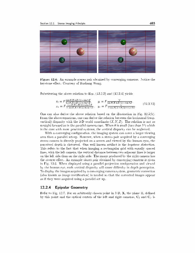
Section 12.2. Stereo Imaging Principle 403
Figure 12.6. An example stereo pair obtained by converging cameras. Notice thekeystone e�ect. Courtesy of Rushang Wang.
Substituting the above relation to Eqs. (12.2.2) and (12.2.4) yields
xl = Fcos �(X+B=2)�sin �Z
sin �(X+B=2)+cos �Z; yl = F Y
sin �(X+B=2)+cos �Z;
xr = Fcos �(X�B=2)+sin �Z
� sin �(X�B=2)+cos �Z; yr = F Y
� sin �(X�B=2)+cos �Z:
(12.2.12)
One can also derive the above relation based on the illustration in Fig. 12.5(b).From the above equations, one can derive the relation between the horizontal (resp.vertical) disparity with the 3-D world coordinate (X;Y; Z). The relation is not asstraight forward as in the parallel camera case. When � is small (less than 1o) whichis the case with most practical systems, the vertical disparity can be neglected.
With a converging con�guration, the imaging system can cover a larger viewingarea than a parallel set-up. However, when a stereo pair acquired by a convergingstereo camera is directly projected on a screen and viewed by the human eyes, theperceived depth is distorted. One well known artifact is the keystone distortion.This refers to the fact that when imaging a rectangular grid with equally spacedlines, with the left camera, the vertical distance between two adjacent lines is largeron the left side than on the right side. The image produced by the right camera hasthe reverse e�ect. An example stereo pair obtained by converging cameras is givenin Fig. 12.6. When displayed using a parallel projection con�guration and viewedby the human eye, such vertical disparity will cause diÆculty in depth perception.To display the images acquired by a converging camera system, geometric correction(also known as image recti�cation) is needed so that the corrected images appearas if they were acquired using a parallel set-up.
12.2.4 Epipolar Geometry
Refer to Fig. 12.7. For an arbitrarily chosen point in 3-D, X, the plane �, de�nedby this point and the optical centers of the left and right cameras, Cl and Cr is
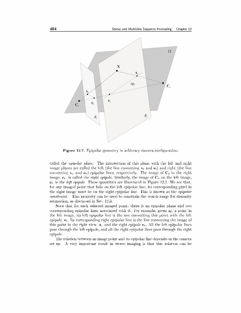
404 Stereo and Multiview Sequence Processing Chapter 12
X
xl
xr
er
elC
l
Cr
Rl
Rr
�
epr
Figure 12.7. Epipolar geometry in arbitrary camera con�guration.
called the epipolar plane. The intersection of this plane with the left and rightimage planes are called the left (the line connecting xl and el) and right (the lineconnecting xr and er) epipolar lines, respectively. The image of Cl in the rightimage, er, is called the right epipole. Similarly, the image of Cr on the left image,el, is the left epipole. These quantities are illustrated in Figure 12.7. We see that,for any imaged point that falls on the left epipolar line, its corresponding pixel inthe right image must be on the right epipolar line. This is known as the epipolar
constraint. This property can be used to constrain the search range for disparityestimation, as discussed in Sec. 12.3.
Note that for each selected imaged point, there is an epipolar plane and twocorresponding epipolar lines associated with it. For example, given xl, a point inthe left image, its left epipolar line is the one connecting this point with the leftepipole, el. Its corresponding right epipolar line is the line connecting the image ofthis point in the right view, xr and the right epipole er: All the left epipolar linespass through the left epipole, and all the right epipolar lines pass through the rightepipole.
The relation between an image point and its epipolar line depends on the cameraset-up. A very important result in stereo imaging is that this relation can be
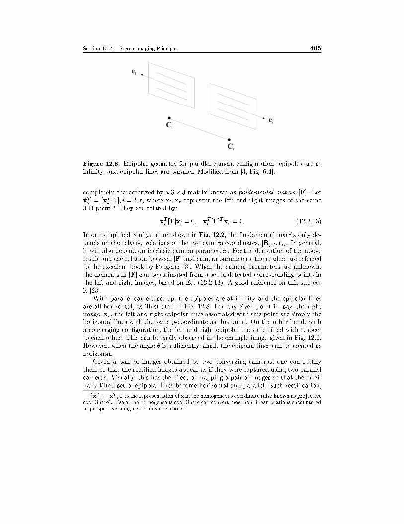
Section 12.2. Stereo Imaging Principle 405
el
Cl
er
Cr
Figure 12.8. Epipolar geometry for parallel camera con�guration: epipoles are atin�nity, and epipolar lines are parallel. Modi�ed from [3, Fig. 6.4].
completely characterized by a 3� 3 matrix known as fundamental matrix, [F]. Let~xTi = [xTi ; 1]; i = l; r; where xl;xr represent the left and right images of the same3-D point.5 They are related by:
~xTr [F]~xl = 0; ~xTl [F]T ~xr = 0: (12.2.13)
In our simpli�ed con�guration shown in Fig. 12.2, the fundamental matrix only de-pends on the relative relations of the two camera coordinates, [R]rl; trl. In general,it will also depend on intrinsic camera parameters. For the derivation of the aboveresult and the relation between [F] and camera parameters, the readers are referredto the excellent book by Faugeras [3]. When the camera parameters are unknown,the elements in [F] can be estimated from a set of detected corresponding points inthe left and right images, based on Eq. (12.2.13). A good reference on this subjectis [23].
With parallel camera set-up, the epipoles are at in�nity and the epipolar linesare all horizontal, as illustrated in Fig. 12.8. For any given point in, say, the rightimage, xr, the left and right epipolar lines associated with this point are simply thehorizontal lines with the same y-coordinate as this point. On the other hand, witha converging con�guration, the left and right epipolar lines are tilted with respectto each other. This can be easily observed in the example image given in Fig. 12.6.However, when the angle � is suÆciently small, the epipolar lines can be treated ashorizontal.
Given a pair of images obtained by two converging cameras, one can rectifythem so that the recti�ed images appear as if they were captured using two parallelcameras. Visually, this has the e�ect of mapping a pair of images so that the origi-nally tilted set of epipolar lines become horizontal and parallel. Such recti�cation,
5~xT = [xT ; 1] is the representation of x in the homogeneous coordinate (also known as projective
coordinate). Use of the homogeneous coordinate can convert most non-linear relations encountered
in perspective imaging to linear relations.
406 Stereo and Multiview Sequence Processing Chapter 12
for example, would greatly simplify the disparity estimation problem. It is alsoneeded for displaying these images by a parallel projection system. Recall from theprevious discussion, the epipolar constraint is completely characterized by the fun-damental matrix relating the two cameras. Therefore, the key to the recti�cationprocess is to determine the fundamental matrix. In practice, the camera con�gura-tion parameters may not be known exactly, so that the fundamental matrix mustbe determined from the corresponding feature points in the two given images. Adiscussion on camera calibration and recti�cation techniques is beyond the scope ofthis chapter. The readers are referred to [19, 3] for a good treatment of this subject.
12.3 Disparity Estimation
As introduced in the previous section, disparity refers to the displacement betweenthe 2-D coordinates in the left and right image planes of a 3-D point in the imagedscene. As shown in Sec. 12.2, from the disparity associated with two correspondingpoints in a stereo image pair, one can derive the depth associated with the under-lying 3-D point and consequently its complete 3-D coordinate in the real world.For this reason, disparity estimation is an essential step in any 3-D image/videoprocessing system. It is also important for generating intermediate views betweengiven views.
Disparity estimation problem is similar to the motion estimation problem in thatboth require establishment of the correspondence between pixels in two images. Innon-feature-based approach, for every point in one image, the task is to determineits corresponding point in the other image, or mark it as being occluded in the otherimage. For feature-based approach, the task is to �rst detect certain feature pointsin one image, and then �nd their corresponding positions in the other. For motionestimation, the two images di�er in time; whereas in disparity estimation, the twoimages are taken at the same time but from di�erent camera view angles.
Disparity estimation tends to be more complex and challenging than motionestimation. First, usually only a limited number of objects move in the scene sothat the MV's are zero for most pixels. In stereo imaging, however, almost allpixels have non-zero disparities, except those pixels that are very far away from theimage plane. Secondly, the range of MV's is usually quite limited, whereas the DVcan be very large for objects close to the camera. For example, with CCIR 601video, the MV's usually do not exceed a few pixels, whereas the DV's can reach40-50 pixels in the horizontal direction and up to 5 pixels in the vertical direction(assuming a slightly convergent camera is used) [6]. Obviously if one were to use asearch technique similar to the block matching algorithm for motion estimation, thesearch region must be greatly increased. The blocking artifacts also become morevisible because the block-wise constant model does not approximate the disparityvariation well.
The general approach to disparity estimation is very similar to motion estima-tion, except that there are more physically induced constraints in disparity �elds, asdescribed below. Basically, one needs to set up an objective function that measures
Section 12.3. Disparity Estimation 407
the error between a given view and its predicted version from the other view usingdisparity compensated prediction (DCP). If we assume that the disparity �eld issmooth, then some smoothness measures can be added to the objective function.These smoothness constraints should be relaxed at object boundaries or occludedregions. The estimated parameters are further subjected to some physical con-straints. The di�erence between di�erent approaches lie in the parameterizationof the disparity �eld as well as the search method. In the following, we �rst de-scribe some important constraints that are useful for disparity estimation. We thenpresent several estimation methods.
12.3.1 Constraints on Disparity Distribution
The disparity vectors are constrained by the camera geometry and the continuityof the object surface. These constraints, if used judiciously, can be very helpful indisparity estimation.
Epipolar Constraint
Given a stereo imaging con�guration, the epipolar constraint refers to the fact thatthe corresponding pixels in a stereo pair always lie on respective epipolar lines.Recall that if the fundamental matrix is known, then, given any point in, say, theright image, one can determine the epipolar line in the left image using Eq. (12.2.13),which de�nes all possible locations of this point in the left image. Therefore, oneonly needs to search along this line.
For the parallel camera con�guration, the epipolar lines are parallel to horizontalscan lines of the images, so that one can constrain the search within the horizontalline that the right image point is located. When the camera con�guration is non-parallel, although one can con�ne the search to the epipolar lines corresponding tothe actual camera set-up, one simpler approach is to �rst map the left and rightimages into a parallel con�guration, and then apply the procedure for the parallelcon�guration [21]. In either case, one must �rst estimate the camera geometry pa-rameters or the fundamental matrix, which is required for determining the epipolarlines or for reprojection.
Uni-Directionality with Parallel Camera
As shown in Sec. 12.2.2, with the parallel camera con�guration, the disparity vec-tor only has horizontal component and is always positive (i.e., the left horizontalcoordinate is always larger than the right one).
Ordering Constraint
Assuming opacity of the imaged objects, the relative positions of di�erent points inan object are the same in both views of the scene, i.e., a feature point left of anotherin the left view lies also on the left in the right view. Let xr;1 and xr;2 representtwo points in the right image on the same horizontal line and assume xr;1 < xr;2.
408 Stereo and Multiview Sequence Processing Chapter 12
Then by requiring xl;1 < xl;2, we have dx;2 < dx;1+xl;2�xl;1, which constrains thesearch range for dx;2 given the previously estimated dx;1:
12.3.2 Models for the Disparity Function
Disparity is a deterministic function of the depth, for a given camera con�guration.Given a model for the actual surface function, one can derive the correspondingmodel for the disparity function. Such a model is very helpful for disparity estima-tion.
Consider the simplest case when the surface of the imaged scene can be approx-imated by a plane so that
Z(X;Y ) = aX + bY + c: (12.3.1)
Using (12.2.6) and (12.2.7), we can rewrite Z in terms of the right image coordinates:
Z(xr; yr) = a
�Zxr
F�
B
2
�+ b
Zyr
F+ c (12.3.2)
or
Z(xr; yr) =c+ aB=2
1� axr=F � byr=F: (12.3.3)
We can see that the surface function varies non-linearly in terms of image coordi-nates. Substituting the above result into (12.2.8) yields:
dx(xr; yr) =1
c=B + a=2(F + axr + byr): (12.3.4)
Therefore, the disparity function is aÆne in the image coordinate when the surface
is a plane.
In reality, the entire surface (i.e., the depth distribution) of the imaged scenecannot be approximated well by a plane. However, it usually can be divided intosmall patches so that each patch is approximately planar. Using the above result, wecan model the disparity function over each patch as aÆne. The disparity estimationproblem can then be turned into estimating three aÆne parameters for each patch,which is equivalent to estimating the disparity (dx only) at three corner points(nodes) of each patch. If we represent the entire surface by a triangular mesh,then the disparity estimation problem can be reduced to estimating the disparityat nodal points. The disparity function within each patch can then be interpolatedfrom the nodal points using the aÆne model.
Using similar approaches, one can also derive the disparity model for higherorder (curved) surfaces. Such parametric models can be very helpful for disparityestimation.
12.3.3 Block-Based Approach
This approach assumes that the disparity function over each small block of thereference view can be described by a constant or a low order polynomial. The

Section 12.3. Disparity Estimation 409
constant disparity or the polynomial coeÆcients are determined by minimizing theerror between the two views after warping based on the estimated disparity function(i.e., disparity compensation). Either exhaustive or gradient-descent search meth-ods used for block-based motion estimation can be applied. But the search shouldbe constrained properly, using the constraints described in Sec. 12.3.1. In the spe-cial case that the disparity is assumed to be constant, only a single horizontal shiftneeds to be searched, and only in one direction, positive or negative, dependingon which view is used as reference. However, compared to motion estimation, thesearch range should be much larger, if the depth variation in the imaged scene isrelatively large or the baseline separation between cameras is large. To overcomethe diÆculty associated with the potentially very large disparity value, a hierarchi-cal search strategy, as the one described in Sec. 6.9, should be used. A good reviewof block-based estimation methods can be found in [20].
Unlike motion estimation, where the block-wise constant model is fairly accuratefor a large number of blocks, this model is only appropriate when the surface patchcorresponding to the block is a at surface that is parallel with the imaging plane,which is rarely the case. On the other hand, the aÆne model is quite good whenthe block size is suÆciently small. In this case, the surface patch corresponding toeach block is approximately at, and as shown in Sec. 12.3.2, the disparity functionover a planar patch is well described by an aÆne function.
12.3.4 2-D Mesh-Based Approach
Instead of using a block-wise constant model, the mesh-based approach describedfor motion estimation can also be applied to disparity estimation. In this case, one�rst applies a mesh in a reference view, say the left view, and tries to �nd the cor-responding nodal positions in the right view. Note that each pair of corresponding2-D mesh elements can be considered as the projections of a 3-D surface patch onthe left and right images, as shown in Fig. 12.9. As with motion estimation, it isbest to parameterize the disparity function by the nodal displacement between theleft and right views, rather than polynomial coeÆcients in aÆne or bilinear models.One can estimate the nodal disparities by minimizing the disparity compensatedprediction error between corresponding elements, similar to the mesh-based motionestimation method (Sec. 6.6). When the underlying images are obtained with aparallel set-up, only horizontal disparities need to be searched.
One such approach is described in [21]. As shown in Fig. 12.9, the left view isdescribed by a rectangular mesh, and the nodes in the right view are shifted horizon-tally with respect to the corresponding nodes in the left view. The disparity functionwithin each element is modeled as bilinear, so that the 3-D patch corresponding tothis element is a curved surface. To determine the horizontal disparity at each node,the disparity compensation error summed over the four elements attached to thisnode is minimized. Instead of performing exhaustive search, a gradient-based fastalgorithm is used.
Figure 12.10 compares the disparity estimation result for a sample stereo image
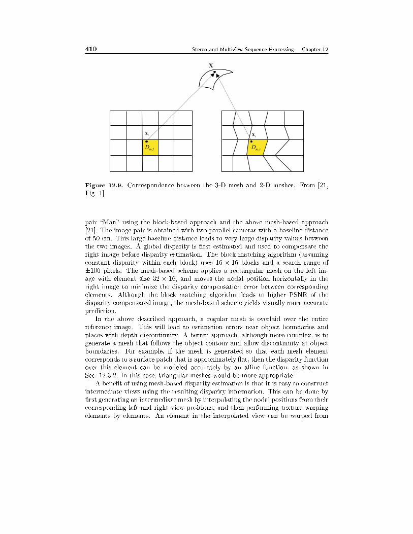
410 Stereo and Multiview Sequence Processing Chapter 12
lmD , rm
D ,
X
xl xr
Figure 12.9. Correspondence between the 3-D mesh and 2-D meshes. From [21,Fig. 1].
pair \Man" using the block-based approach and the above mesh-based approach[21]. The image pair is obtained with two parallel cameras with a baseline distanceof 50-cm. This large baseline distance leads to very large disparity values betweenthe two images. A global disparity is �rst estimated and used to compensate theright image before disparity estimation. The block matching algorithm (assumingconstant disparity within each block) uses 16 � 16 blocks and a search range of�100 pixels. The mesh-based scheme applies a rectangular mesh on the left im-age with element size 32 � 16, and moves the nodal position horizontally in theright image to minimize the disparity compensation error between correspondingelements. Although the block matching algorithm leads to higher PSNR of thedisparity compensated image, the mesh-based scheme yields visually more accurateprediction.
In the above described approach, a regular mesh is overlaid over the entirereference image. This will lead to estimation errors near object boundaries andplaces with depth discontinuity. A better approach, although more complex, is togenerate a mesh that follows the object contour and allow discontinuity at objectboundaries. For example, if the mesh is generated so that each mesh elementcorresponds to a surface patch that is approximately at, then the disparity functionover this element can be modeled accurately by an aÆne function, as shown inSec. 12.3.2. In this case, triangular meshes would be more appropriate.
A bene�t of using mesh-based disparity estimation is that it is easy to constructintermediate views using the resulting disparity information. This can be done by�rst generating an intermediate mesh by interpolating the nodal positions from theircorresponding left and right view positions, and then performing texture warpingelements by elements. An element in the interpolated view can be warped from
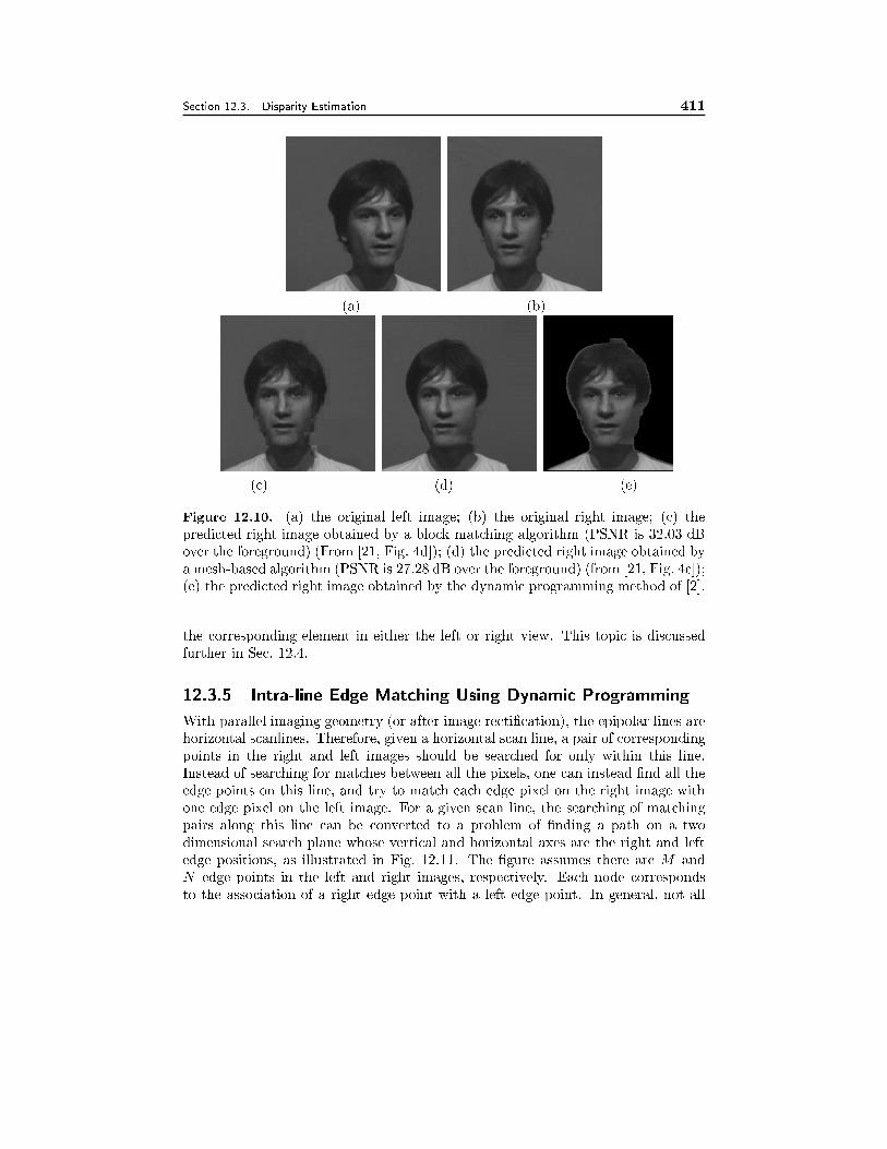
Section 12.3. Disparity Estimation 411
(a) (b)
(c) (d) (e)
Figure 12.10. (a) the original left image; (b) the original right image; (c) thepredicted right image obtained by a block matching algorithm (PSNR is 32.03 dBover the foreground) (From [21, Fig. 4d]); (d) the predicted right image obtained bya mesh-based algorithm (PSNR is 27.28 dB over the foreground) (from [21, Fig. 4c]);(e) the predicted right image obtained by the dynamic programming method of [2].
the corresponding element in either the left or right view. This topic is discussedfurther in Sec. 12.4.
12.3.5 Intra-line Edge Matching Using Dynamic Programming
With parallel imaging geometry (or after image recti�cation), the epipolar lines arehorizontal scanlines. Therefore, given a horizontal scan line, a pair of correspondingpoints in the right and left images should be searched for only within this line.Instead of searching for matches between all the pixels, one can instead �nd all theedge points on this line, and try to match each edge pixel on the right image withone edge pixel on the left image. For a given scan line, the searching of matchingpairs along this line can be converted to a problem of �nding a path on a twodimensional search plane whose vertical and horizontal axes are the right and leftedge positions, as illustrated in Fig. 12.11. The �gure assumes there are M andN edge points in the left and right images, respectively. Each node correspondsto the association of a right edge point with a left edge point. In general, not all
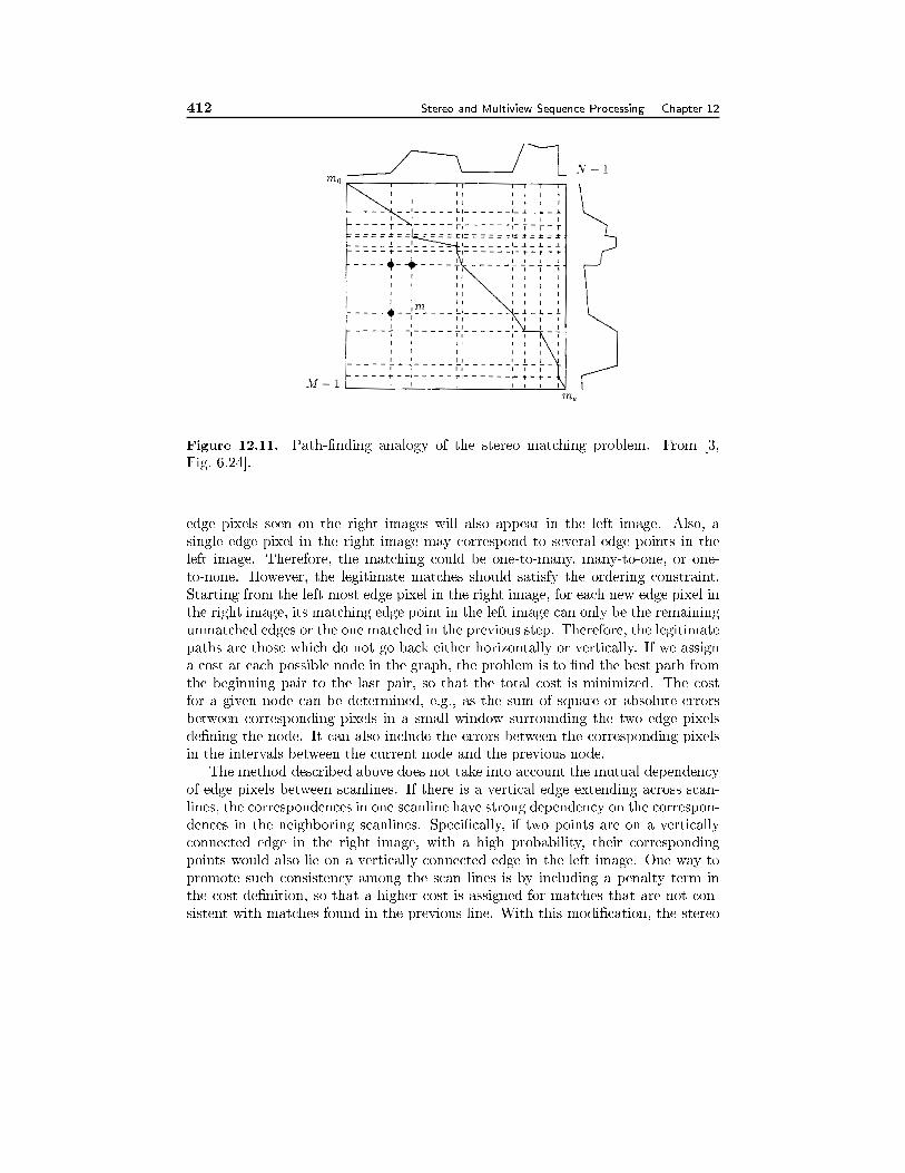
412 Stereo and Multiview Sequence Processing Chapter 12
Figure 12.11. Path-�nding analogy of the stereo matching problem. From [3,Fig. 6.24].
edge pixels seen on the right images will also appear in the left image. Also, asingle edge pixel in the right image may correspond to several edge points in theleft image. Therefore, the matching could be one-to-many, many-to-one, or one-to-none. However, the legitimate matches should satisfy the ordering constraint.Starting from the left most edge pixel in the right image, for each new edge pixel inthe right image, its matching edge point in the left image can only be the remainingunmatched edges or the one matched in the previous step. Therefore, the legitimatepaths are those which do not go back either horizontally or vertically. If we assigna cost at each possible node in the graph, the problem is to �nd the best path fromthe beginning pair to the last pair, so that the total cost is minimized. The costfor a given node can be determined, e.g., as the sum of square or absolute errorsbetween corresponding pixels in a small window surrounding the two edge pixelsde�ning the node. It can also include the errors between the corresponding pixelsin the intervals between the current node and the previous node.
The method described above does not take into account the mutual dependencyof edge pixels between scanlines. If there is a vertical edge extending across scan-lines, the correspondences in one scanline have strong dependency on the correspon-dences in the neighboring scanlines. Speci�cally, if two points are on a verticallyconnected edge in the right image, with a high probability, their correspondingpoints would also lie on a vertically connected edge in the left image. One way topromote such consistency among the scan lines is by including a penalty term inthe cost de�nition, so that a higher cost is assigned for matches that are not con-sistent with matches found in the previous line. With this modi�cation, the stereo
Section 12.3. Disparity Estimation 413
matching problem can be cast as that of �nding a surface that best satis�es theintra-scanline matches and inter-scanline consistency. Here the matching surface isde�ned by stacking 2-D matching paths.
Ohta and Kanade [10] �rst proposed to cast the disparity estimation problemas the surface matching program outlined above. Furthermore, they developed afast search algorithm using the dynamic programming method. The original workof Ohta and Kanade only considered the constraint imposed by edges along thevertical direction. Falkenhagen extended this scheme to consider more complicated2-D constraints [2]. Figure 12.10(e) show the predicted right image for \Man" usingthis method.6
12.3.6 Joint Structure and Motion Estimation
The previous discussions have focused on the estimation of the disparity functionfrom a pair of stereoscopic views obtained at the same time. From the disparityfunction, one can derive the structure (i.e., spatial distribution) of the imaged scene,as described in Sec. 12.2. This would allow one to reconstruct the 3-D surface ofthe imaged object. With stereo sequences, one is interested in the estimation of notonly structure at a given frame, but also 3-D motion between frames. The mostchallenging problem is to estimate structure and motion jointly.
One common approach to this problem is to model the surface of the imagedobject with a 3-D mesh (also known as a wireframe). Then the structure and motionestimation problem is to �nd the 3-D coordinates of all the nodes in a startingframe, and the 3-D nodal displacements between successive frames. Note that the3-D mesh will project to 2-D meshes in the left and right images, as illustrated inFig. 12.12. To determine the initial 3-D mesh, one can �rst construct a 2-D meshin one view, and then �nd the corresponding nodal positions in the other view.This can be solved using the mesh-based disparity estimation method describedin Sec. 12.3.4. From the disparities between corresponding nodes, one can thendetermine the 3-D positions of all the nodes. For the produced 3-D mesh to �twith the actual object surface, the initial 2-D mesh has to be adapted to the objectboundary and each element should correspond to a at patch. This however requiresthe knowledge of the object structure. Therefore, it is important to obtain a goodobject segmentation based on the stereo views. Also, an iterative procedure may benecessary, each time starting with a new 2-D mesh adapted based on the previousestimate of the object structure. To determine the 3-D nodal displacements, onecan determine 2-D nodal displacements in both views, by minimizing the motion-compensated prediction error between two adjacent frames of the same view, aswell as disparity-compensated prediction error between two views at the same frametime. The main diÆculty in both structure and motion estimation lies in how tohandle occluded regions, including regions seen only in one view at the same frametime, and regions disappearing or newly appearing over time. For research paperson this topic, see [5, 7, 18].
6Courtesy of Fatih Porikli, who implemented the method of [2] with slight modi�cations.
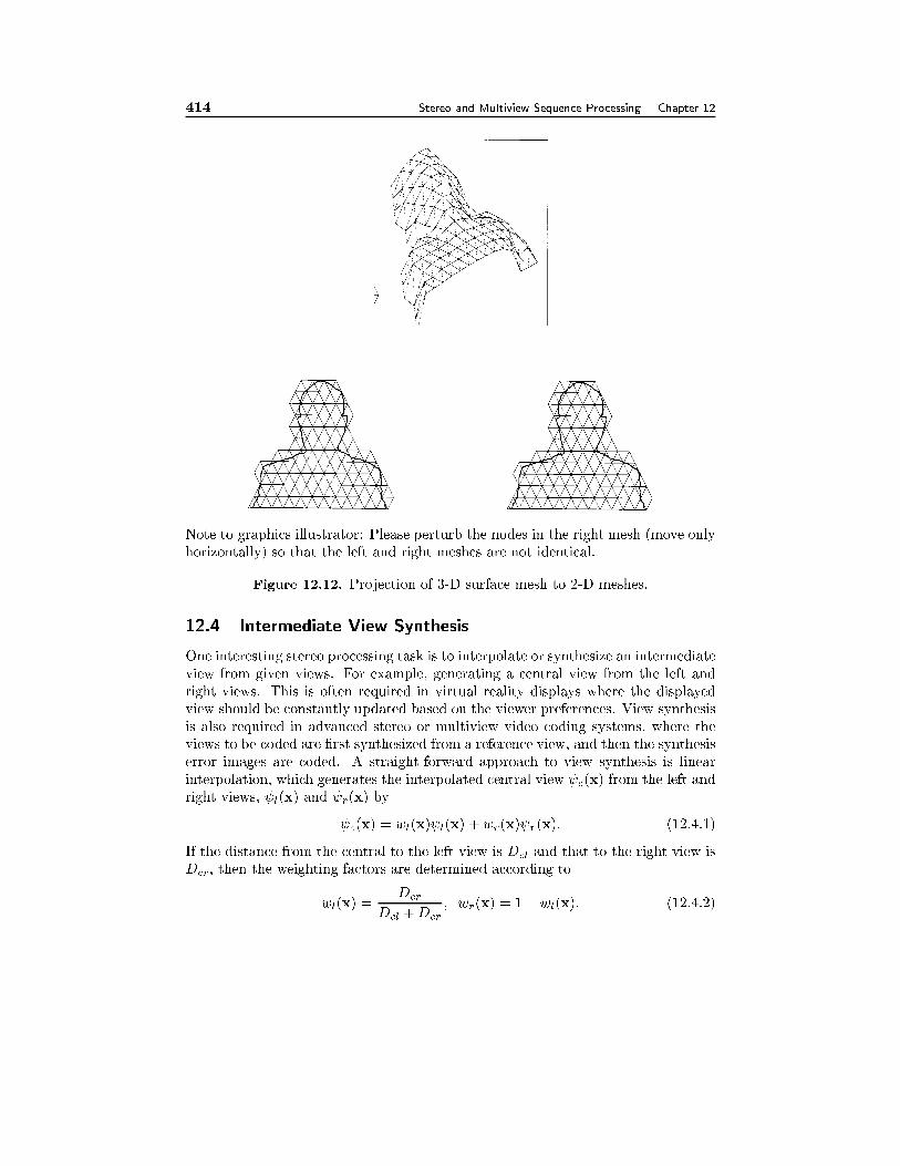
414 Stereo and Multiview Sequence Processing Chapter 12
Note to graphics illustrator: Please perturb the nodes in the right mesh (move onlyhorizontally) so that the left and right meshes are not identical.
Figure 12.12. Projection of 3-D surface mesh to 2-D meshes.
12.4 Intermediate View Synthesis
One interesting stereo processing task is to interpolate or synthesize an intermediateview from given views. For example, generating a central view from the left andright views. This is often required in virtual reality displays where the displayedview should be constantly updated based on the viewer preferences. View synthesisis also required in advanced stereo or multiview video coding systems, where theviews to be coded are �rst synthesized from a reference view, and then the synthesiserror images are coded. A straight-forward approach to view synthesis is linearinterpolation, which generates the interpolated central view c(x) from the left andright views, l(x) and r(x) by
c(x) = wl(x) l(x) + wr(x) r(x): (12.4.1)
If the distance from the central to the left view is Dcl and that to the right view isDcr, then the weighting factors are determined according to
wl(x) =Dcr
Dcl +Dcr
; wr(x) = 1� wl(x): (12.4.2)
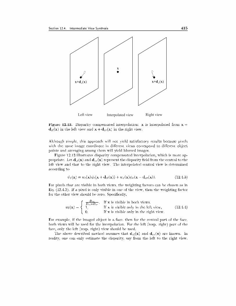
Section 12.4. Intermediate View Synthesis 415
x
x+d xcl( ) x+d xcr( )
Left view Right viewInterpolated view
Figure 12.13. Disparity compensated interpolation: x is interpolated from x +dcl(x) in the left view and x+ dcr(x) in the right view.
Although simple, this approach will not yield satisfactory results because pixelswith the same image coordinate in di�erent views correspond to di�erent objectpoints and averaging among them will yield blurred images.
Figure 12.13 illustrates disparity compensated interpolation, which is more ap-propriate. Let dcl(x) and dcr(x) represent the disparity �eld from the central to theleft view and that to the right view. The interpolated central view is determinedaccording to
c(x) = wl(x) l(x+ dcl(x)) + wr(x) r(x+ dcr(x)): (12.4.3)
For pixels that are visible in both views, the weighting factors can be chosen as inEq. (12.4.2). If a pixel is only visible in one of the view, then the weighting factorfor the other view should be zero. Speci�cally,
wl(x) =
8<:
Dcr
Dcl+Dcr
; If x is visible in both views,
1; If x is visible only in the left view,0; If x is visible only in the right view.
(12.4.4)
For example, if the imaged object is a face, then for the central part of the face,both views will be used for the interpolation. For the left (resp. right) part of theface, only the left (resp. right) view should be used.
The above described method assumes that dcl(x) and dcr(x) are known. Inreality, one can only estimate the disparity, say from the left to the right view,
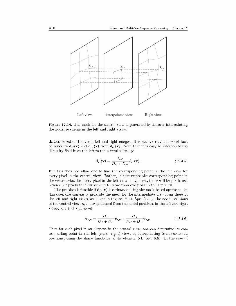
416 Stereo and Multiview Sequence Processing Chapter 12
xc, nxl, n xr, n
Left view Right viewInterpolated view
Figure 12.14. The mesh for the central view is generated by linearly interpolatingthe nodal positions in the left and right views.
dlr(x); based on the given left and right images. It is not a straight forward taskto generate dcl(x) and dcr(x) from dlr(x). Note that it is easy to interpolate thedisparity �eld from the left to the central view, by
dlc(x) =Dcl
Dcl +Dcr
dlr(x): (12.4.5)
But this does not allow one to �nd the corresponding point in the left view forevery pixel in the central view. Rather, it determines the corresponding point inthe central view for every pixel in the left view. In general, there will be pixels notcovered, or pixels that correspond to more than one pixel in the left view.
The problem is feasible if dlr(x) is estimated using the mesh-based approach. Inthis case, one can easily generate the mesh for the intermediate view from those inthe left and right views, as shown in Figure 12.14. Speci�cally, the nodal positionsin the central view, xc;n are generated from the nodal positions in the left and rightviews, xl;n and xr;n using
xc;n =Dcr
Dcl +Dcr
xl;n +Dcl
Dcl +Dcr
xr;n: (12.4.6)
Then for each pixel in an element in the central view, one can determine its cor-responding point in the left (resp. right) view, by interpolating from the nodalpositions, using the shape functions of the element (cf. Sec. 6.6). In the case of
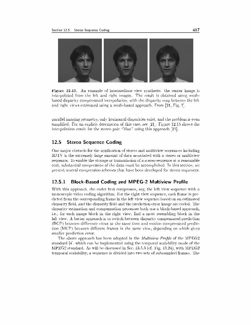
Section 12.5. Stereo Sequence Coding 417
Figure 12.15. An example of intermediate view synthesis: the center image isinterpolated from the left and right images. The result is obtained using mesh-based disparity compensated interpolation, with the disparity map between the leftand right views estimated using a mesh-based approach. From [21, Fig. 7].
parallel imaging geometry, only horizontal disparities exist, and the problem is evensimpli�ed. For an explicit description of this case, see [21]. Figure 12.15 shows theinterpolation result for the stereo pair \Man" using this approach [21].
12.5 Stereo Sequence Coding
One major obstacle for the application of stereo and multiview sequences including3DTV is the extremely large amount of data associated with a stereo or multiviewsequence. To enable the storage or transmission of a stereo sequence at a reasonablecost, substantial compression of the data must be accomplished. In this section, wepresent several compression schemes that have been developed for stereo sequences.
12.5.1 Block-Based Coding and MPEG-2 Multiview Pro�le
With this approach, the coder �rst compresses, say, the left view sequence with amonoscopic video coding algorithm. For the right view sequence, each frame is pre-dicted from the corresponding frame in the left view sequence based on an estimateddisparity �eld, and the disparity �eld and the prediction error image are coded. Thedisparity estimation and compensation processes both use a block-based approach,i.e., for each image block in the right view, �nd a most resembling block in theleft view. A better approach is to switch between disparity compensated prediction(DCP) between di�erence views at the same time and motion compensated predic-tion (MCP) between di�erent frames in the same view, depending on which givessmaller prediction error.
The above approach has been adopted in the Multiview Pro�le of the MPEG2standard [4], which can be implemented using the temporal scalability mode of theMPEG2 standard. As will be discussed in Sec. 13.5.3 (cf. Fig. 13.24), with MPEG2temporal scalability, a sequence is divided into two sets of subsampled frames. The
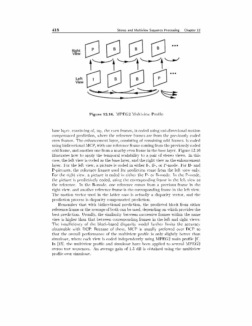
418 Stereo and Multiview Sequence Processing Chapter 12
Figure 12.16. MPEG2 Multiview Pro�le
base layer, consisting of, say, the even frames, is coded using uni-directional motioncompensated prediction, where the reference frames are from the previously codedeven frames. The enhancement layer, consisting of remaining odd frames, is codedusing bidirectional MCP, with one reference frame coming from the previously codedodd frame, and another one from a nearby even frame in the base layer. Figure 12.16illustrates how to apply the temporal scalability to a pair of stereo views. In thiscase, the left view is coded as the base layer, and the right view as the enhancementlayer. For the left view, a picture is coded in either I-, B-, or P-mode. For B- andP-pictures, the reference frames used for prediction come from the left view only.For the right view, a picture is coded in either the P- or B-mode. In the P-mode,the picture is predictively coded, using the corresponding frame in the left view asthe reference. In the B-mode, one reference comes from a previous frame in theright view, and another reference frame is the corresponding frame in the left view.The motion vector used in the latter case is actually a disparity vector, and theprediction process is disparity compensated prediction.
Remember that with bidirectional prediction, the predicted block from eitherreference frame or the average of both can be used, depending on which provides thebest prediction. Usually, the similarity between successive frames within the sameview is higher than that between corresponding frames in the left and right views.The insuÆciency of the block-based disparity model further limits the accuracyobtainable with DCP. Because of these, MCP is usually preferred over DCP sothat the overall performance of the multiview pro�le is only slightly better thansimulcast, where each view is coded independently using MPEG2 main pro�le [8].In [13], the multiview pro�le and simulcast have been applied to several MPEG2stereo test sequences. An average gain of 1.5 dB is obtained using the multiviewpro�le over simulcast.
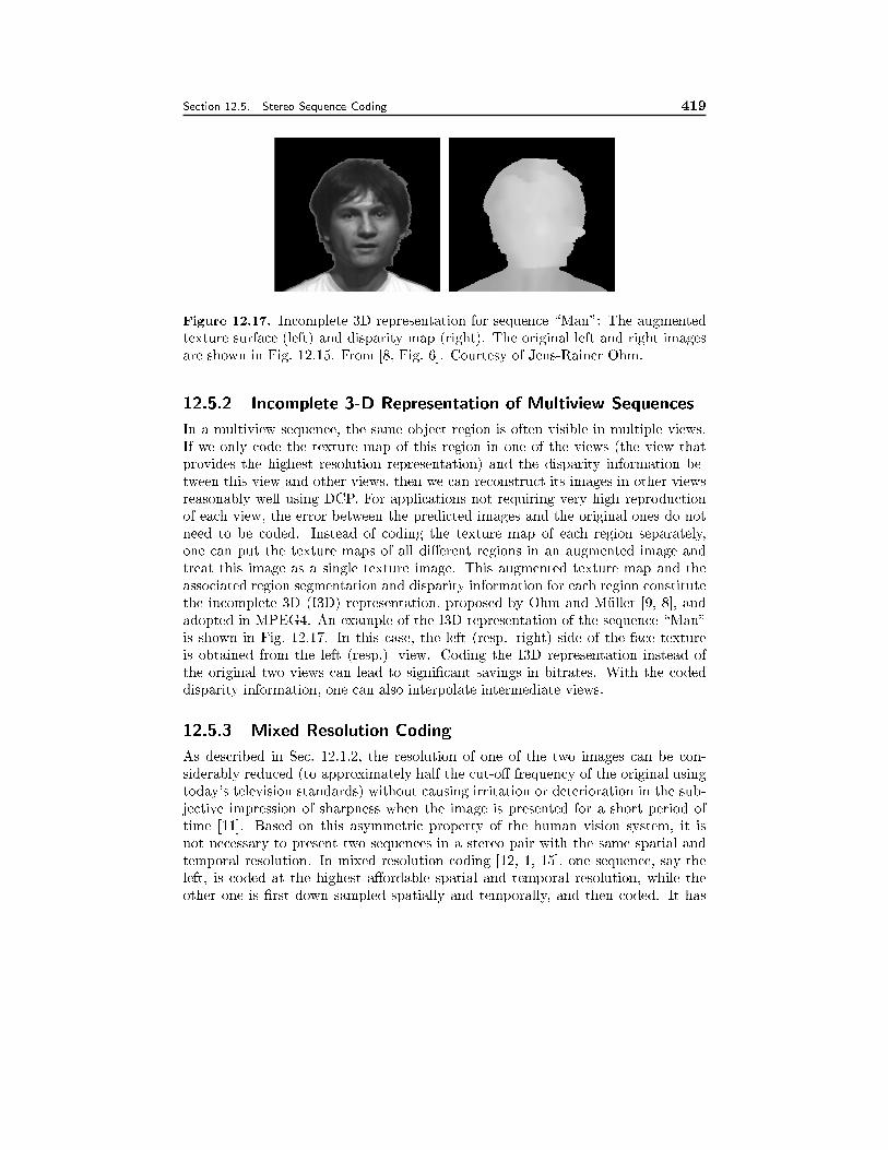
Section 12.5. Stereo Sequence Coding 419
Figure 12.17. Incomplete 3D representation for sequence \Man": The augmentedtexture surface (left) and disparity map (right). The original left and right imagesare shown in Fig. 12.15. From [8, Fig. 6]. Courtesy of Jens-Rainer Ohm.
12.5.2 Incomplete 3-D Representation of Multiview Sequences
In a multiview sequence, the same object region is often visible in multiple views.If we only code the texture map of this region in one of the views (the view thatprovides the highest resolution representation) and the disparity information be-tween this view and other views, then we can reconstruct its images in other viewsreasonably well using DCP. For applications not requiring very high reproductionof each view, the error between the predicted images and the original ones do notneed to be coded. Instead of coding the texture map of each region separately,one can put the texture maps of all di�erent regions in an augmented image andtreat this image as a single texture image. This augmented texture map and theassociated region segmentation and disparity information for each region constitutethe incomplete 3D (I3D) representation, proposed by Ohm and M�uller [9, 8], andadopted in MPEG4. An example of the I3D representation of the sequence \Man"is shown in Fig. 12.17. In this case, the left (resp. right) side of the face textureis obtained from the left (resp.) view. Coding the I3D representation instead ofthe original two views can lead to signi�cant savings in bitrates. With the codeddisparity information, one can also interpolate intermediate views.
12.5.3 Mixed Resolution Coding
As described in Sec. 12.1.2, the resolution of one of the two images can be con-siderably reduced (to approximately half the cut-o� frequency of the original usingtoday's television standards) without causing irritation or deterioration in the sub-jective impression of sharpness when the image is presented for a short period oftime [11]. Based on this asymmetric property of the human vision system, it isnot necessary to present two sequences in a stereo pair with the same spatial andtemporal resolution. In mixed resolution coding [12, 1, 15], one sequence, say theleft, is coded at the highest a�ordable spatial and temporal resolution, while theother one is �rst down sampled spatially and temporally, and then coded. It has
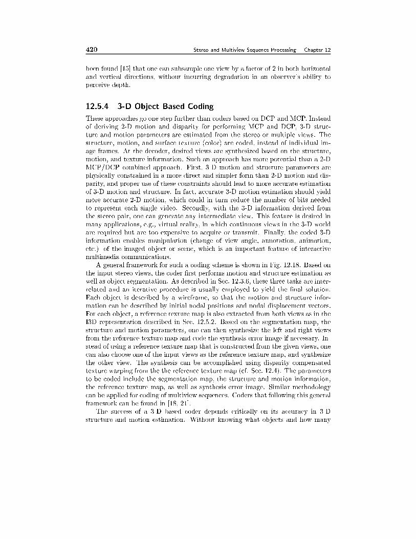
420 Stereo and Multiview Sequence Processing Chapter 12
been found [15] that one can subsample one view by a factor of 2 in both horizontaland vertical directions, without incurring degradation in an observer's ability toperceive depth.
12.5.4 3-D Object Based Coding
These approaches go one step further than coders based on DCP and MCP. Insteadof deriving 2-D motion and disparity for performing MCP and DCP, 3-D struc-ture and motion parameters are estimated from the stereo or multiple views. Thestructure, motion, and surface texture (color) are coded, instead of individual im-age frames. At the decoder, desired views are synthesized based on the structure,motion, and texture information. Such an approach has more potential than a 2-DMCP/DCP combined approach. First, 3-D motion and structure parameters arephysically constrained in a more direct and simpler form than 2-D motion and dis-parity, and proper use of these constraints should lead to more accurate estimationof 3-D motion and structure. In fact, accurate 3-D motion estimation should yieldmore accurate 2-D motion, which could in turn reduce the number of bits neededto represent each single video. Secondly, with the 3-D information derived fromthe stereo pair, one can generate any intermediate view. This feature is desired inmany applications, e.g., virtual reality, in which continuous views in the 3-D worldare required but are too expensive to acquire or transmit. Finally, the coded 3-Dinformation enables manipulation (change of view angle, annotation, animation,etc.) of the imaged object or scene, which is an important feature of interactivemultimedia communications.
A general framework for such a coding scheme is shown in Fig. 12.18. Based onthe input stereo views, the coder �rst performs motion and structure estimation aswell as object segmentation. As described in Sec. 12.3.6, these three tasks are inter-related and an iterative procedure is usually employed to yield the �nal solution.Each object is described by a wireframe, so that the motion and structure infor-mation can be described by initial nodal positions and nodal displacement vectors.For each object, a reference texture map is also extracted from both views as in theI3D representation described in Sec. 12.5.2. Based on the segmentation map, thestructure and motion parameters, one can then synthesize the left and right viewsfrom the reference texture map and code the synthesis error image if necessary. In-stead of using a reference texture map that is constructed from the given views, onecan also choose one of the input views as the reference texture map, and synthesizethe other view. The synthesis can be accomplished using disparity compensatedtexture warping from the the reference texture map (cf. Sec. 12.4). The parametersto be coded include the segmentation map, the structure and motion information,the reference texture map, as well as synthesis error image. Similar methodologycan be applied for coding of multiview sequences. Coders that following this generalframework can be found in [18, 21].
The success of a 3-D based coder depends critically on its accuracy in 3-Dstructure and motion estimation. Without knowing what objects and how many
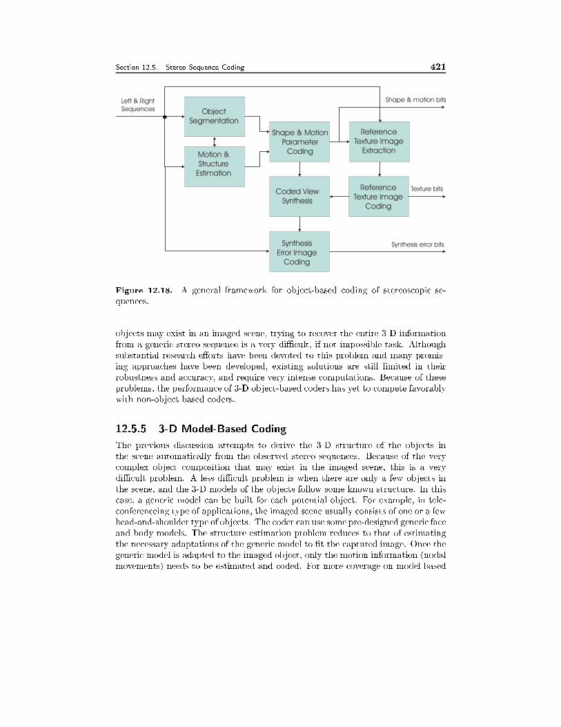
Section 12.5. Stereo Sequence Coding 421
Object
Segmentation
Motion &
Structure
Estimation
Reference
Texture Image
Extraction
Coded View
Synthesis
Synthesis
Error Image
Coding
Reference
Texture Image
Coding
Shape & Motion
Parameter
Coding
Left & Right
Sequences
Shape & motion bits
Synthesis error bits
Texture bits
Figure 12.18. A general framework for object-based coding of stereoscopic se-quences.
objects may exist in an imaged scene, trying to recover the entire 3-D informationfrom a generic stereo sequence is a very diÆcult, if not impossible task. Althoughsubstantial research e�orts have been devoted to this problem and many promis-ing approaches have been developed, existing solutions are still limited in theirrobustness and accuracy, and require very intense computations. Because of theseproblems, the performance of 3-D object-based coders has yet to compete favorablywith non-object based coders.
12.5.5 3-D Model-Based Coding
The previous discussion attempts to derive the 3-D structure of the objects inthe scene automatically from the observed stereo sequences. Because of the verycomplex object composition that may exist in the imaged scene, this is a verydiÆcult problem. A less diÆcult problem is when there are only a few objects inthe scene, and the 3-D models of the objects follow some known structure. In thiscase, a generic model can be built for each potential object. For example, in tele-conferenceing type of applications, the imaged scene usually consists of one or a fewhead-and-shoulder type of objects. The coder can use some pre-designed generic faceand body models. The structure estimation problem reduces to that of estimatingthe necessary adaptations of the generic model to �t the captured image. Once thegeneric model is adapted to the imaged object, only the motion information (nodalmovements) needs to be estimated and coded. For more coverage on model-based
422 Stereo and Multiview Sequence Processing Chapter 12
coding, see Chap. 10.
12.6 Summary
Stereo imaging principle
With stereo imaging, the images of a 3-D point on two di�erent views are displacedwith respect to each other and it is this disparity between the two image positionsthat enables the recovery of the depth information of the 3-D point. The mostgeneral relation between depth and image positions is given by Eq. (12.2.5). For themost popular parallel camera con�guration, this is reduced to the famous inverserelationship between disparity and depth (Eq. 12.2.8). The relation between theleft and right image positions of the same object point is described by the epipolargeometry (Fig. 12.7, Eq. 12.2.13).
Disparity Estimation
Disparity estimation is similar to motion estimation in that one needs to �nd corre-sponding points in two di�erent images, and hence can be accomplished using similarapproaches, including block-based and mesh-based methods. Compared to motionestimation, disparity estimation can be helped with more physical constraints. Themost important one is the epipolar constraint, which says for any point in a rightimage, its corresponding point in the left image must fall on the epipolar line. Forparallel set-up, this means that corresponding points in two images are on the samehorizontal line.
Disparity estimation is a fundamental step for recovering 3-D structure andmotion of imaged objects from a stereo sequence. To achieve this goal, disparityestimation must be done in conjunction with object segmentation, 3-D modelingusing wireframes, and detection and treatment of occluded regions.
Stereo and multiview sequence coding
There are generally two types of approach. The �rst type is waveform-based: itcombines disparity compensated prediction and motion compensated prediction,and codes the prediction error image and the dispairty/motion vectors. The secondtype is object-based: it tries to recover the 3-D structure and motion of the imagedobject, and codes these information directly. The second approach has the potentialof achieving very high compression ratios, for simply structured scenes. It alsofacilitates the synthesis of any intermediate view at the decoder.
12.7 Problems
12.1 What are the pros and cons of parallel vs. converging camera con�gurationfor stereo imaging?
Section 12.7. Problems 423
12.2 Derive the horizontal and vertical disparity values, dx(xr; yy); dy(xr ; yr), inthe converging camera con�guration. Show that the vertical disparity is zerofor X = 0 or Y = 0: Also derive how to determine the 3-D position fromdx(xr ; yr); dy(xr ; yr).
12.3 What is the fundamental matrix [F] for (a) parallel and (b) converging cameracon�guration?
12.4 For a curved surface, Z = aX + bY + cXY + d; what is the parameterizedform of the disparity function?
12.5 When the baseline between two parallel cameras is large, the horizontal dis-parities are very large. In this case, it is better to �rst estimate a globalhorizontal disparity value, before applying block-wise or mesh-based disparityestimation. This global disparity can be found by �nding a global horizontalshift between the two image that will yield the least error after shifting. Writea program to estimate the global disparity between a stereo pair.
12.6 Implement (in C or Matlab) a hierarchical block matching algorithm for dis-parity estimation for the case of parallel imaging geometry (only horizontaldisparity needs to be searched). Evaluate its performance over a stereo imagepair. You should �rst estimate the global disparity and then apply the blockmatching algorithm to the images after global disparity compensation.
12.7 Implement the mesh-based approach for disparity estimation for the case ofparallel imaging geometry. For simplicity, use a regular square mesh over thereference view. Compare its performance for the same stereo pair to the blockmatching algorithm.
12.8 Implement the dynamic programming scheme for disparity estimation de-scribed in [10]. Evaluate its performance over a stereo image pair. Compare itsperformance to the block-matching algorithm and the mesh-based approach.
12.9 Generate an intermediate view between a stereo pair acquired by parallelcameras. Compare two approaches: a) linear interpolation; and b) disparity-compensated interpolation using the mesh-based approach (Sec. 12.4). Ideally,you should estimate the disparity values using the mesh-based approach. Ifyou choose to use the simpler block-based approach, then you can assume thedisparity found for each block is the disparity at the center of the block, andall the block centers are the nodes in the mesh for the reference view.
12.10 Implement a stereo image coder using block-based disparity compensation.Code one image (reference view) using the DCT-base method (Sec. 9.1.7). Forthe other image, for each block, �nd its prediction using block-based disparity,and then code the error block using the DCT-based approach.
424 Stereo and Multiview Sequence Processing Chapter 12
12.11 Implement a stereo video coder using block-based disparity compensationand motion compensation. Code one view (reference view) using the hybridcoding method (Sec. 9.3.1). Using unidirectional prediction only for simplicity.For the other view, for each block in a frame, it is estimated both usingmotion compensation from the previous frame in this view, and using disparitycompensation from the same frame in the reference view. Use either theaverage of the two predictions or one of the predictions, depending on theprediction errors. The prediction error is then coded using the DCT-basedmethod.
12.8 Bibliography
[1] I. Dinstein et al. Compression of stereo images and the evaluation of its e�ectson 3-D perception. In Proc. EEE Conf. Applications of Digital Image Processing,1989.
[2] L. Falkenhagen. Depth estimation from stereoscopic image pairs assuming piece-wise continuos surfaces. In Y. Paker and S. Wilbur, editors, Image Processing for
Broadcast and Video Production, pages 115{127. Springer, Great Britain, 1994.
[3] O. Faugeras. Three-Dimensional Computer Vision - A Geometric Viewpoint.The MIT Press, 1993.
[4] ISO/IEC. IS 13818-2 AMD3: MPEG-2 multiview pro�le, Sept. 1996.
[5] R. Koch. Dynamic 3D scene analysis through synthesis feedback control. IEEETrans. Pattern Anal. Machine Intell., 15:556{568, 1993.
[6] A. Kopernik, R. Sand, and B. Choquet. The future of three-dimensional TV.In Signal processing of HDTV. Elsevier Science Publishers B.V., 1993.
[7] S. Malassiotis and M. G. Strintzis. Model-based joint motion and structure esti-mation from stereo images. Computer Vision, and Image Understanding, 65(1):79{94, Jan. 1997.
[8] J.-R. Ohm. Encoding and reconstruction of multiview video objects. IEEE
Signal Processing Magazine, 16(3):47{54, May 1999.
[9] J.-R. Ohm and K. Muller. Incomplete 3D | multiview representation of videoobjects. IEEE Trans. Circuits Syst. for Video Technology, 9(2):389{400, Mar.1999.
[10] Y. Ohta and T. Kanade. Stereo by intra- and inter-scanline search using dy-namic programming. IEEE Trans. Pattern Anal. Machine Intell., PAMI-7:139{145, 1985.
[11] S. Pastoor. 3D-television: A survey of recent research results on subjectiverequirements. Signal Processing: Image Commun., 4:21{32, 1991.
Section 12.8. Bibliography 425
[12] M. Perkins. Data compression of stereopairs. IEEE Trans. Comm., 4:684{696,1992.
[13] A. Puri, V. Kollarits, and B. Haskell. Stereoscopic video compression usingtemporal scalability. In SPIE Conf. Visual Commun. Image Processing (VCIP95),volume SPIE-2501, pages 745{756, Taipei, Taiwan, 1995.
[14] J. Ross and J. H. Hogeben. Short-term memory in stereopsis. Vision Res.,14:1195{1201, 1974.
[15] S. Sethuraman, M. W. Siegel, and A. G. Jordan. A multiresolution frameworkfor stereoscopic image sequence compression. In Proc. IEEE Int. Conf. Image
Processing (ICIP94), Austin, 1994.
[16] I. Sexton and P. Surman. Stereoscopic and autostereoscopic display systems- an in-depth review of past, present, and future technologies. IEEE Signal Pro-
cessing Magazine, 16(3):85{99, May 1999.
[17] Stereographics, Inc. Perceiving stereoscopic images.http://www.stereographics.com/html/chapter 2.html.
[18] M. G. Strintzis and S. Malassiotis. Object-based coding of stereoscopic and 3Dimage sequences. IEEE Signal Processing Magazine, 16(3):14{28, May 1999.
[19] R. Y. Tsai. A versatile camera calibration technique for high-accuracy 3Dmachine vision metrology using o�-the-shelf TV cameras and lenses. IEEE Journal
of Robotics and Automation, RA-3:323{344, August 1987.
[20] D. Tzovaras, M. S. Strintzis, and H. Sahinoglou. Evaluation of multiresolu-tion techniques for motion and disparity estimation. Signal Processing: Image
Commun., 6(1):59{67, June 1994.
[21] R. Wang and Y. Wang. Multiview video sequence analysis, compression, andvirtual viewpoint synthesis. IEEE Trans. Circuits Syst. for Video Technology,10(3):397{410, April 2000.
[22] J. Weng, T. S. Huang, and N. Ahuja. Motion and structure from image se-
quences. Springer-Verlag, 1993.
[23] Z. Zhang. Determining the epipolar geometry and its uncertainty: A review.Technical report, INRIA, July 1996.
Chapter 13
VIDEO COMPRESSION
STANDARDS
Digital video communication is a complex and compute intensive process that re-
quires many people to receive video signals from di�erent sources. There are mainly
three classes of devices that we use for digital video communications today:
� Digital television sets or settop boxes are mainly designed to receive video
signals from di�erent content providers. These devices rely on one �xed video
decoding algorithm that is implemented in hardware or in a combination of
hardware and a programmable Reduced Instruction Set Computers (RISC)
processor or Digital Signal Processor (DSP). Currently, there are no means
provided for uploading a new algorithm once the hardware is deployed to the
customer.
� Videophones are usually implemented on DSPs with hardware acceleration
for some compute intensive parts of the video coding and decoding algorithm
such as DCT and motion estimation. Usually, the set of algorithms used in a
particular videophone cannot be replaced.
� Personal Computers are the most exible and most expensive platform for dig-
ital video communication. While a PC with a high-end Pentium III processor
is able to decode DVDs, the software is usually preinstalled with the operat-
ing system in order to avoid hardware and driver problems. Video decoders
for streaming video may be updated using automatic software download and
installation, as done by commercial software such as Real Player, Windows
Media Player, Apple Quicktime and Microsoft Netmeeting.
Digital video communications standards were mainly developed for digital tele-
vision and video phones in order to enable industry to provide consumers with a
bandwidth eÆcient terminal at an a�ordable price. We describe the standards orga-
nizations, the meaning of compatibility and applications for video coding standards
in Section 13.1. We begin the description of actual standards with the ITU video
coding standards H.261 and H.263 (Sec. 13.2) for interactive video communications.
426
Section 13.1. Standardization 427
In Section 13.3 we present the standards H.323 and H.324 that de�ne multimedia
terminals for audiovisual communications. Within ISO, the Moving Picture Experts
Group (MPEG) de�ned MPEG-1 (Sec. 13.4) and MPEG-2 (Sec. 13.5) for entertain-
ment and digital TV. MPEG-4 (Sec. 13.6) is the �rst international standard that
does not only standardize audio and video communications but also graphics for
use in entertainment and interactive multimedia services. All standards describe
the syntax and semantics of a bitstream. Section 13.7 presents an overview over
the organization of a bitstream as used by H.261, H.263, MPEG-1,-2, and MPEG-4.
Finally, we give a brief description of the on-going MPEG-7 standardization activity
(Sec. 13.8), which intends to standardize the interface for describing the content of
an audiovisual document.
13.1 Standardization
Developing an International Standard requires collaboration between many parters
from di�erent countries, and an organization that is able to support the standard-
ization process as well as to enforce the standards. In Section 13.1.1 we describe
the organizations like ITU and ISO. In Section 13.1.2, the meaning of compatibility
is de�ned. Section 13.1.3 brie y describes the workings of a standardization body.
In Section 13.1.4 applications for video communications are listed.
13.1.1 Standards Organizations
Standards are required if we want multiple terminals from di�erent vendors to
exchange information or to receive information from a common source like a TV
broadcast station. Standardization organizations have their roots in the telecom
industry creating ITU and trade creating ISO.
ITU
The telecom industry has established a long record of setting international standards
[7]. At the beginning of electric telegraphy in the 19th century, telegraph lines did
not cross national frontiers because each country used a di�erent system and each
had its own telegraph code to safeguard the secrecy of its military and political
telegraph messages. Messages had to be transcribed, translated and handed over at
frontiers before being retransmitted over the telegraph network of the neighboring
country. The �rst International Telegraph Convention was signed in May 1865
and harmonized the di�erent systems used. This event marked the birth of the
International Telecommunication Union (ITU).
Following the invention of the telephone and the subsequent expansion of tele-
phony, the Telegraph Union began, in 1885, to draw up international rules for
telephony. In 1906 the �rst International Radiotelegraph Convention was signed.
Subsequently, several committees were set up for establishing international stan-
dards including the International Telephone Consultative Committee (CCIF) in
1924, the International Telegraph Consultative Committee (CCIT) in 1925, and
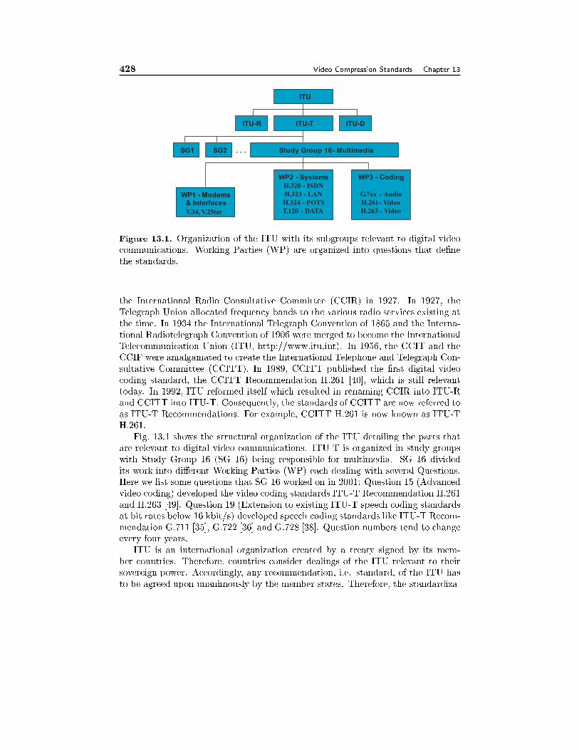
428 Video Compression Standards Chapter 13
ITU
ITU-TITU-R
SG1 Study Group 16- Multimedia
ITU-D
SG2 . . .
WP1 - Modems& Interfaces
V.34, V.25ter
WP3 - Coding
G.7xx - Audio
H.261- Video
H.263 - Video
WP2 - Systems
H.320 - ISDN
H.323 - LAN
H.324 - POTS
T.120 - DATA
Figure 13.1. Organization of the ITU with its subgroups relevant to digital video
communications. Working Parties (WP) are organized into questions that de�ne
the standards.
the International Radio Consultative Committee (CCIR) in 1927. In 1927, the
Telegraph Union allocated frequency bands to the various radio services existing at
the time. In 1934 the International Telegraph Convention of 1865 and the Interna-
tional Radiotelegraph Convention of 1906 were merged to become the International
Telecommunication Union (ITU, http://www.itu.int). In 1956, the CCIT and the
CCIF were amalgamated to create the International Telephone and Telegraph Con-
sultative Committee (CCITT). In 1989, CCITT published the �rst digital video
coding standard, the CCITT Recommendation H.261 [40], which is still relevant
today. In 1992, ITU reformed itself which resulted in renaming CCIR into ITU-R
and CCITT into ITU-T. Consequently, the standards of CCITT are now referred to
as ITU-T Recommendations. For example, CCITT H.261 is now known as ITU-T
H.261.
Fig. 13.1 shows the structural organization of the ITU detailing the parts that
are relevant to digital video communications. ITU-T is organized in study groups
with Study Group 16 (SG 16) being responsible for multimedia. SG 16 divided
its work into di�erent Working Parties (WP) each dealing with several Questions.
Here we list some questions that SG 16 worked on in 2001: Question 15 (Advanced
video coding) developed the video coding standards ITU-T Recommendation H.261
and H.263 [49]. Question 19 (Extension to existing ITU-T speech coding standards
at bit rates below 16 kbit/s) developed speech coding standards like ITU-T Recom-
mendation G.711 [35], G.722 [36] and G.728 [38]. Question numbers tend to change
every four years.
ITU is an international organization created by a treaty signed by its mem-
ber countries. Therefore, countries consider dealings of the ITU relevant to their
sovereign power. Accordingly, any recommendation, i.e. standard, of the ITU has
to be agreed upon unanimously by the member states. Therefore, the standardiza-
Section 13.1. Standardization 429
tion process in the ITU is often not able to keep up with the progress in modern
technology. Sometimes, the process of reaching unanimous decisions does not work
and ITU recommends regional standards like 7 bit or 8 bit representation of digital
speech in the USA and Europe, respectively. As far as mobile telephony is concerned
ITU did not play a leading role. In the USA there is not even a national mobile
telephony standard, as every operator is free to choose a standard of his own liking.
This contrasts with the approach adopted in Europe where the GSM standard is
so successful that it is expanding all over the world, USA included. With UMTS
(so-called 3rd generation mobile) the ITU-T is retaking its original role of developer
of global mobile telecommunication standards.
ISO
The need to establish international standards developed with the growth of trade
[7]. The International Electrotechnical Commission (IEC) was founded in 1906 to
prepare and publish international standards for all electrical, electronic and related
technologies. The IEC is currently responsible for standards of such communication
means as "receivers", audio and video recording systems, audio-visual equipment,
currently all grouped in TC 100 (Audio, Video and Multimedia Systems and Equip-
ment). International standardization in other �elds and particularly in mechanical
engineering was the concern of the International Federation of the National Stan-
dardizing Associations (ISA), set up in 1926. ISA's activities ceased in 1942 but
a new international organization called International Organization for Standard-
ization (ISO) began to operate again in 1947 with the objective "to facilitate the
international coordination and uni�cation of industrial standards". All computer-
related activities are currently in the Joint ISO/IEC Technical Committee 1 (JTC 1)
on Information Technology. This TC has achieved a very large size. About 1/3 of
all ISO and IEC standards work is done in JTC 1.
The subcommitees SC 24 (Computer Graphics and Image Processing) and SC 29
(Coding of Audio, Picture, Multimedia and Hypermedia Information) are of interest
to multimedia communications. Whereas SC24 de�nes computer graphics standards
like VRML, SC29 developed the well known audiovisual communication standards
MPEG-1, MPEG-2 and MPEG-4 (Fig. 13.2). The standards were developed at
meetings that between 200 and 400 delegates from industry, research institutes and
universities attended.
ISO is an agency of the United Nations since 1947. ISO and IEC have the status
of private not-for-pro�t companies established according to the Swiss Civil Code.
Similarly to ITU, ISO requires consensus in order to publish a standard. ISO also
fails sometimes to establish truly international standards as can be seen with digital
TV. While the same video decoder (MPEG-2 Video) is used worldwide, the audio
representation is di�erent in the US and in Europe.
Both ISO (www.iso.ch) and ITU are in constant competition with industry.
While ISO and ITU have been very successful in de�ning widely used audio and
video coding standards, they were less successful in de�ning transport of multimedia
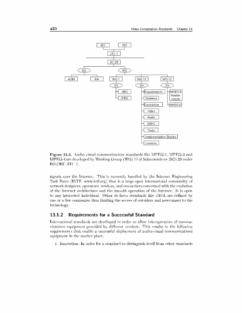
430 Video Compression Standards Chapter 13
Figure 13.2. Audio visual communications standards like MPEG-1, MPEG-2 and
MPEG-4 are developed byWorking Group (WG) 11 of Subcommittee (SC) 29 under
ISO/IEC JTC 1.
signals over the Internet. This is currently handled by the Internet Engineering
Task Force (IETF, www.ietf.org) that is a large open international community of
network designers, operators, vendors, and researchers concerned with the evolution
of the Internet architecture and the smooth operation of the Internet. It is open
to any interested individual. Other de-facto standards like JAVA are de�ned by
one or a few companies thus limiting the access of outsiders and newcomers to the
technology.
13.1.2 Requirements for a Successful Standard
International standards are developed in order to allow interoperation of commu-
nications equipment provided by di�erent vendors. This results in the following
requirements that enable a successful deployment of audio-visual communications
equipment in the market place.
1. Innovation: In order for a standard to distinguish itself from other standards
Section 13.1. Standardization 431
or widely accepted industry standards, it has to provide a signi�cant amount
of innovation. Innovation in the context of video coding means that the
standard provides new functionalities like broadcast-quality interlaced digi-
tal video, video on CDROM or improved compression. If the only distinction
of a new standard is better compression, the standard should provide at least
an improvement that is visible to the consumer and non-expert, before its in-
troduction makes sense commercially. This usually translates to a gain of 3dB
in PSNR of the compressed video at a generally acceptable picture quality.
2. Competition: Standards should not prevent competition between di�erent
manufactures. Therefore, standards speci�cations need to be open and avail-
able to everyone. Free software for encoders and decoders also helps to pro-
mote a standard. Furthermore, a standard should only de�ne the syntax and
semantics of a bitstream, i.e. a standard de�nes how a decoder works. Bit-
stream generation is not standardized. Although the development of bitstream
syntax and semantics requires to have an encoder and a decoder, the standard
does not de�ne the encoder. Therefore, manufactures of standards-compliant
terminals can compete not only about price but also about additional fea-
tures like postprocessing of the decoded media and more importantly about
encoder performance. In video encoding, major di�erences result from motion
estimation, scene change handling, rate control and optimal bit allocation.
3. Transmission and storage media independent: A content provider should be
able to transmit or store the digitally encoded content independent of the
network or storage media. As a consequence of this requirement, we use audio
and video standards to encode the audiovisual information. Then we use a
systems standard to format the audio and video bitstreams into a format
that is suitable for the selected network or storage system. The systems
standard speci�es the packetization, multiplexing and packet header syntax
for delivering the audio and video bitstreams. The separation of transmission
media and media coding usually creates overhead for certain applications. For
example, we cannot exploit the advantages of joint source/channel coding.
4. Forward compatibility: A new standard should be able to understand the
bitstreams of prior standards, i.e. a new video coding standard like H.263 [49]
should be able to decode bitstreams according to the previous video coding
standard H.261 [40]. Forward compatibility ensures that new products can be
gradually introduced into the market. The new features of the latest standard
get only used when terminals conforming to the latest standard communicate.
Otherwise, terminals interoperate according to the previous standard.
5. Backward compatibility: A new standard is backward compatible to an older
standard, if the old standard can decode bitstreams of the new standard. A
very important backward compatible standard was the introduction of ana-
log color TV. Black and white receivers were able to receive the color TV
432 Video Compression Standards Chapter 13
signal and display a slightly degraded black and white version of the signal.
Backward compatibility in today's digital video standards can be achieved by
de�ning reserved bits in the bit stream that a decoder can ignore. A new
standard would transmit extra information using these reserved bits of the
old standard. Thus old terminals will be able to decode bitstreams according
to the new standard. Furthermore, they will understand those parts of the
bit stream that comply to the old standard. Backward compatibility can put
severe restrictions on the improvements that a new standard may achieve over
its predecessor. Therefore, backward compatibility is not always implemented
in a new standard.
6. Upward compatibility: A new receiver should be able to decode bitstreams
that were made for similar receivers of a previous or cheaper generation. Up-
ward compatibility is important if an existing standard is extended. A new
HDTV set should be able to receive standard de�nition TV since both re-
ceivers use the same MPEG-2 standard [19].
7. Downward compatibility: An old receiver should be able to receive and de-
code bitstreams for the newer generation receivers. Downward compatibility
is important if an existing standard is extended. This may be achieved by de-
coding only parts of the bitstream which is easily possible if the new bitstream
is sent as a scalable bitstream (Chapter 11).
Obviously, not all of the above requirements are essential for the wide adoption
of a standard. We believe that the most important requirements are innovation,
competition, and forward compatibility in this order. Compatibility is most impor-
tant for devices like TV settop boxes or mobile phones that cannot be upgraded
easily. On the other hand, any multimedia PC today comes with more than ten
software video codecs installed, relaxing the importance of compatible audio and
video coding standards for this kind of terminals.
13.1.3 Standard Development Process
All video coding standards were developed in three phases, competition, convergence,
veri�cation. Fig. 13.3 shows the process for the video coding standard H.261 [40].
The competition phase started in 1984. The standard was published in December
1990 and revised in 1993.
During the competition phase, the application areas and requirements for the
standard are de�ned. Furthermore, experts gather and demonstrate their best
algorithms. Usually, the standardization body issues a Call for Proposals as soon
as the requirements are de�ned in order to solicit input from the entire community.
This phase can be characterized by independently working competing laboratories.
The goal of the convergence phase is to collaboratively reach an agreement on the
coding method. This process starts with a thorough evaluation of the proposals for
the standard. Issues like coding eÆciency, subjective quality, implementation com-
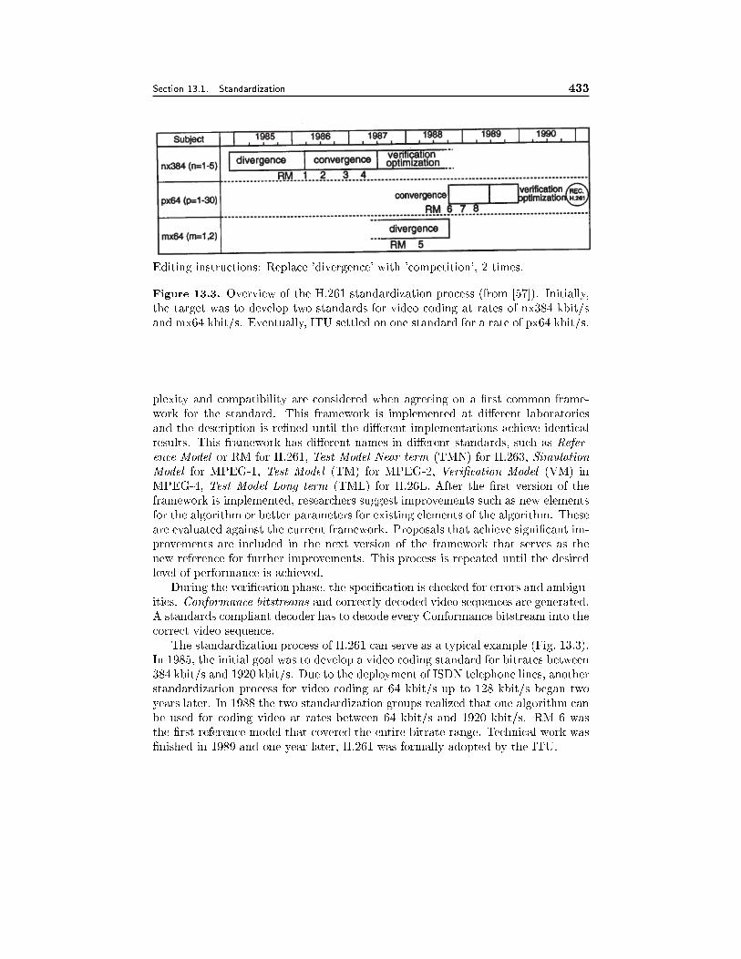
Section 13.1. Standardization 433
Editing instructions: Replace 'divergence' with 'competition', 2 times.
Figure 13.3. Overview of the H.261 standardization process (from [57]). Initially,
the target was to develop two standards for video coding at rates of nx384 kbit/s
and mx64 kbit/s. Eventually, ITU settled on one standard for a rate of px64 kbit/s.
plexity and compatibility are considered when agreeing on a �rst common frame-
work for the standard. This framework is implemented at di�erent laboratories
and the description is re�ned until the di�erent implementations achieve identical
results. This framework has di�erent names in di�erent standards, such as Refer-
ence Model or RM for H.261, Test Model Near term (TMN) for H.263, Simulation
Model for MPEG-1, Test Model (TM) for MPEG-2, Veri�cation Model (VM) in
MPEG-4, Test Model Long term (TML) for H.26L. After the �rst version of the
framework is implemented, researchers suggest improvements such as new elements
for the algorithm or better parameters for existing elements of the algorithm. These
are evaluated against the current framework. Proposals that achieve signi�cant im-
provements are included in the next version of the framework that serves as the
new reference for further improvements. This process is repeated until the desired
level of performance is achieved.
During the veri�cation phase, the speci�cation is checked for errors and ambigu-
ities. Conformance bitstreams and correctly decoded video sequences are generated.
A standards compliant decoder has to decode every Conformance bitstream into the
correct video sequence.
The standardization process of H.261 can serve as a typical example (Fig. 13.3).
In 1985, the initial goal was to develop a video coding standard for bitrates between
384 kbit/s and 1920 kbit/s. Due to the deployment of ISDN telephone lines, another
standardization process for video coding at 64 kbit/s up to 128 kbit/s began two
years later. In 1988 the two standardization groups realized that one algorithm can
be used for coding video at rates between 64 kbit/s and 1920 kbit/s. RM 6 was
the �rst reference model that covered the entire bitrate range. Technical work was
�nished in 1989 and one year later, H.261 was formally adopted by the ITU.
434 Video Compression Standards Chapter 13
13.1.4 Applications for Modern Video Coding Standards
As mentioned previously, there have been several major initiatives in video coding
that have led to a range of video standards for di�erent applications [12].
� Video coding for video teleconferencing, which has led to the ITU standards
called H.261 for ISDN videoconferencing [40], H.263 for video conferencing
over analog telephone lines, desktop and mobile terminals connected to the
Internet [49], and H.262/MPEG-2 video [42][17] for ATM/broadband video-
conferencing.
� Video coding for storing movies on CD-ROM and other consumer video ap-
plications, with about 1:2 Mbits/s allocated to video coding and 256 kbits/s
allocated to audio coding, which led to the initial ISO MPEG-1 standard [16].
Today, MPEG-1 is used for consumer video on CD, Karoke machines, in some
digital camcorders and on the Internet. Some Digital Satellites used MPEG-1
to broadcast TV signals prior to the release of MPEG-2.
� Video coding for broadcast and for storing of digital video on DVD, with on
the order of 2 � 15 Mbits/s allocated to video and audio coding, which led
to the ISO MPEG-2 standard [19] and speci�cations for DVD operations by
the Digital Audio VIsual Council (DAVIC) (www.davic.org) and the DVD
consortium [25]. This work was extended to video coding for HDTV with
bitrates ranging from 15 to 400 Mbits/s allocated to video coding. Applica-
tions include satellite TV, Cable TV, terrestrial broadcast, video editing and
storage. Today, MPEG-2 video is used in every digital settop box. It is also
selected as the video decoder for the American HDTV broadcast system.
� Coding of separate audio-visual objects, both natural and synthetic is stan-
dardized in ISO MPEG-4 [22]. Target applications are Internet video, inter-
active video, content manipulation, professional video, 2D and 3D computer
graphics, and mobile video communications.
In the following sections, we will �rst describe H.261. For H.263, we will highlight
the di�erences from H.261 and compare their coding eÆciency. Then, we will discuss
MPEG-1, MPEG-2 and MPEG-4, again focusing on their di�erences.
13.2 Video Telephony with H.261 and H.263
Video coding at 64 kbit/s was �rst demonstrated at a conference in 1979 [56]. How-
ever, it took more than ten years to be able to de�ne a commercially viable video
coding standard at that rate. The standard H.261 was published in 1990 in order
to enable video conferencing using between one and thirty ISDN channels. At that
time, video conferencing hardware became available from di�erent vendors. Com-
panies like PictureTel that sold video conferencing equipment with a proprietary
algorithm quickly o�ered H.261 as an option. Later, ITU developed the similar
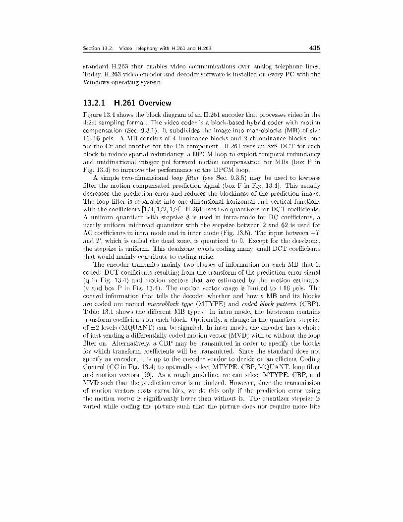
Section 13.2. Video Telephony with H.261 and H.263 435
standard H.263 that enables video communications over analog telephone lines.
Today, H.263 video encoder and decoder software is installed on every PC with the
Windows operating system.
13.2.1 H.261 Overview
Figure 13.4 shows the block diagram of an H.261 encoder that processes video in the
4:2:0 sampling format. The video coder is a block-based hybrid coder with motion
compensation (Sec. 9.3.1). It subdivides the image into macroblocks (MB) of size
16x16 pels. A MB consists of 4 luminance blocks and 2 chrominance blocks, one
for the Cr and another for the Cb component. H.261 uses an 8x8 DCT for each
block to reduce spatial redundancy, a DPCM loop to exploit temporal redundancy
and unidirectional integer pel forward motion compensation for MBs (box P in
Fig. 13.4) to improve the performance of the DPCM loop.
A simple two-dimensional loop �lter (see Sec. 9.3.5) may be used to lowpass
�lter the motion compensated prediction signal (box F in Fig. 13.4). This usually
decreases the prediction error and reduces the blockiness of the prediction image.
The loop �lter is separable into one-dimensional horizontal and vertical functions
with the coeÆcients [1=4; 1=2; 1=4]. H.261 uses two quantizers for DCT coeÆcients.
A uniform quantizer with stepsize 8 is used in intra-mode for DC coeÆcients, a
nearly uniform midtread quantizer with the stepsize between 2 and 62 is used for
AC coeÆcients in intra-mode and in inter-mode (Fig. 13.5). The input between �Tand T , which is called the dead zone, is quantized to 0. Except for the deadzone,
the stepsize is uniform. This deadzone avoids coding many small DCT coeÆcients
that would mainly contribute to coding noise.
The encoder transmits mainly two classes of information for each MB that is
coded: DCT coeÆcients resulting from the transform of the prediction error signal
(q in Fig. 13.4) and motion vectors that are estimated by the motion estimator
(v and box P in Fig. 13.4). The motion vector range is limited to �16 pels. The
control information that tells the decoder whether and how a MB and its blocks
are coded are named macroblock type (MTYPE) and coded block pattern (CBP).
Table 13.1 shows the di�erent MB types. In intra-mode, the bitstream contains
transform coeÆcients for each block. Optionally, a change in the quantizer stepsize
of �2 levels (MQUANT) can be signaled. In inter-mode, the encoder has a choice
of just sending a di�erentially coded motion vector (MVD) with or without the loop
�lter on. Alternatively, a CBP may be transmitted in order to specify the blocks
for which transform coeÆcients will be transmitted. Since the standard does not
specify an encoder, it is up to the encoder vendor to decide on an eÆcient Coding
Control (CC in Fig. 13.4) to optimally select MTYPE, CBP, MQUANT, loop �lter
and motion vectors [69]. As a rough guideline, we can select MTYPE, CBP, and
MVD such that the prediction error is minimized. However, since the transmission
of motion vectors costs extra bits, we do this only if the prediction error using
the motion vector is signi�cantly lower than without it. The quantizer stepsize is
varied while coding the picture such that the picture does not require more bits
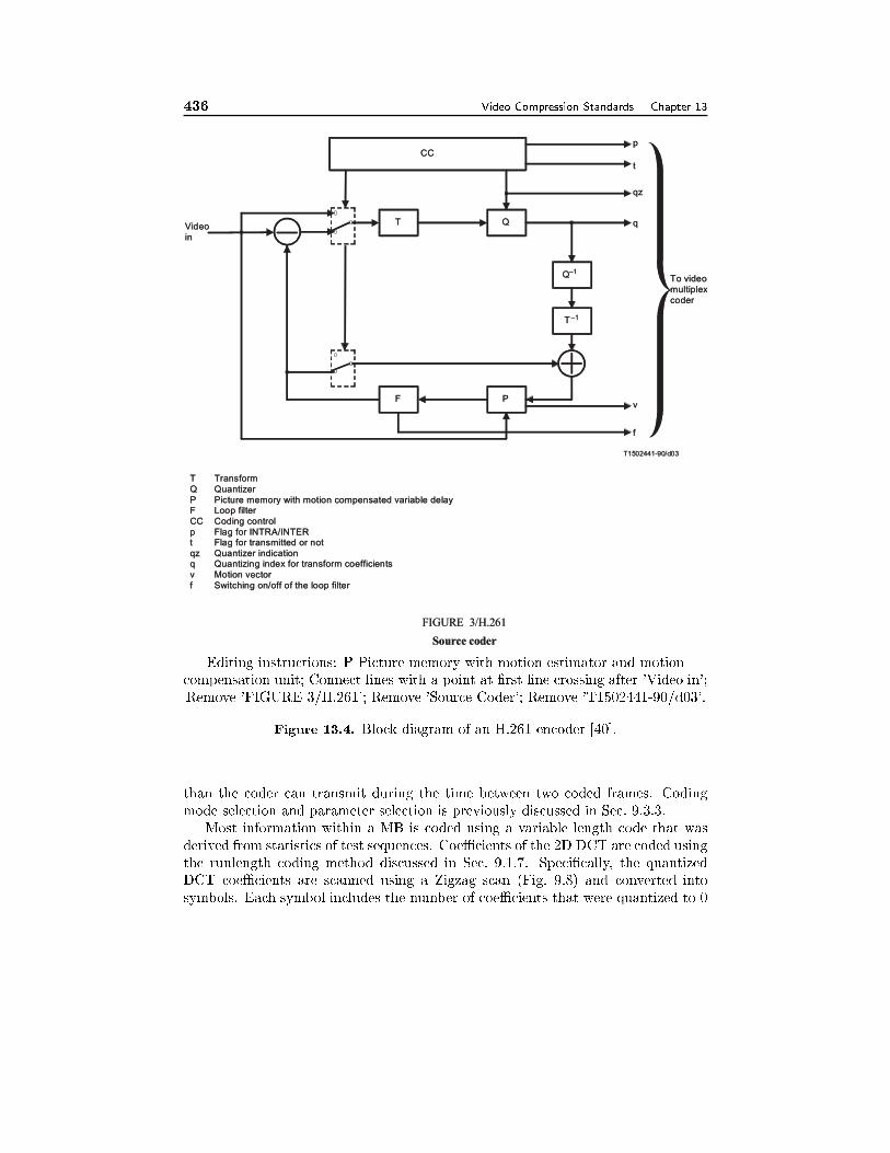
436 Video Compression Standards Chapter 13
T1502441-90/d03
CC
T Q
Q
T
F P
p
t
qz
q
v
f
T
Q
PF
CC
pt
qzq
v
f
Video
in
To video
multiplex
coder
Transform
Quantizer
Picture memory with motion compensated variable delayLoop filter
Coding control
Flag for INTRA/INTERFlag for transmitted or not
Quantizer indicationQuantizing index for transform coefficients
Motion vector
Switching on/off of the loop filter
–1
–1
FIGURE 3/H.261
Source coder
Editing instructions: P Picture memory with motion estimator and motion
compensation unit; Connect lines with a point at �rst line crossing after 'Video in';
Remove 'FIGURE 3/H.261'; Remove 'Source Coder'; Remove 'T1502441-90/d03'.
Figure 13.4. Block diagram of an H.261 encoder [40].
than the coder can transmit during the time between two coded frames. Coding
mode selection and parameter selection is previously discussed in Sec. 9.3.3.
Most information within a MB is coded using a variable length code that was
derived from statistics of test sequences. CoeÆcients of the 2D DCT are coded using
the runlength coding method discussed in Sec. 9.1.7. Speci�cally, the quantized
DCT coeÆcients are scanned using a Zigzag scan (Fig. 9.8) and converted into
symbols. Each symbol includes the number of coeÆcients that were quantized to 0
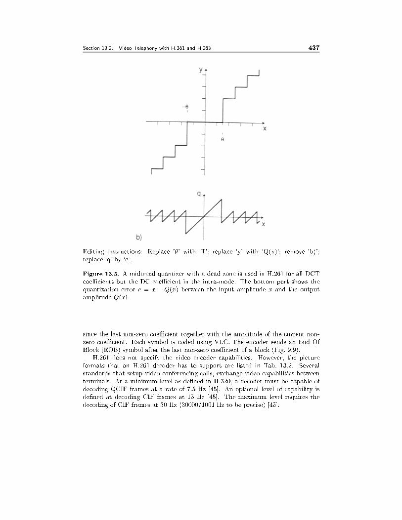
Section 13.2. Video Telephony with H.261 and H.263 437
Editing instructions: Replace '�' with 'T'; replace 'y' with 'Q(x)'; remove 'b)';
replace 'q' by 'e'.
Figure 13.5. A midtread quantizer with a dead zone is used in H.261 for all DCT
coeÆcients but the DC coeÆcient in the intra-mode. The bottom part shows the
quantization error e = x � Q(x) between the input amplitude x and the output
amplitude Q(x).
since the last non-zero coeÆcient together with the amplitude of the current non-
zero coeÆcient. Each symbol is coded using VLC. The encoder sends an End Of
Block (EOB) symbol after the last non-zero coeÆcient of a block (Fig. 9.9).
H.261 does not specify the video encoder capabilities. However, the picture
formats that an H.261 decoder has to support are listed in Tab. 13.2. Several
standards that setup video conferencing calls, exchange video capabilities between
terminals. At a minimum level as de�ned in H.320, a decoder must be capable of
decoding QCIF frames at a rate of 7.5 Hz [45]. An optional level of capability is
de�ned at decoding CIF frames at 15 Hz [45]. The maximum level requires the
decoding of CIF frames at 30 Hz (30000=1001 Hz to be precise) [45].
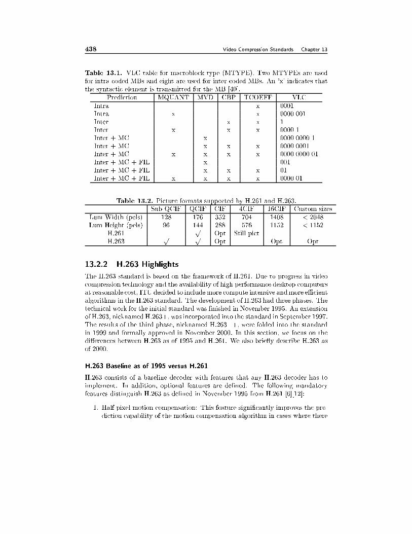
438 Video Compression Standards Chapter 13
Table 13.1. VLC table for macroblock type (MTYPE). Two MTYPEs are used
for intra-coded MBs and eight are used for inter-coded MBs. An 'x' indicates that
the syntactic element is transmitted for the MB [40].
Prediction MQUANT MVD CBP TCOEFF VLC
Intra x 0001
Intra x x 0000 001
Inter x x 1
Inter x x x 0000 1
Inter + MC x 0000 0000 1
Inter + MC x x x 0000 0001
Inter + MC x x x x 0000 0000 01
Inter + MC + FIL x 001
Inter + MC + FIL x x x 01
Inter + MC + FIL x x x x 0000 01
Table 13.2. Picture formats supported by H.261 and H.263.
Sub-QCIF QCIF CIF 4CIF 16CIF Custom sizes
Lum Width (pels) 128 176 352 704 1408 < 2048
Lum Height (pels) 96 144 288 576 1152 < 1152
H.261p
Opt Still pict
H.263p p
Opt Opt Opt
13.2.2 H.263 Highlights
The H.263 standard is based on the framework of H.261. Due to progress in video
compression technology and the availability of high performance desktop computers
at reasonable cost, ITU decided to include more compute intensive and more eÆcient
algorithms in the H.263 standard. The development of H.263 had three phases. The
technical work for the initial standard was �nished in November 1995. An extension
of H.263, nicknamed H.263+, was incorporated into the standard in September 1997.
The results of the third phase, nicknamed H.263++, were folded into the standard
in 1999 and formally approved in November 2000. In this section, we focus on the
di�erences between H.263 as of 1995 and H.261. We also brie y describe H.263 as
of 2000.
H.263 Baseline as of 1995 versus H.261
H.263 consists of a baseline decoder with features that any H.263 decoder has to
implement. In addition, optional features are de�ned. The following mandatory
features distinguish H.263 as de�ned in November 1995 from H.261 [6][12]:
1. Half-pixel motion compensation: This feature signi�cantly improves the pre-
diction capability of the motion compensation algorithm in cases where there
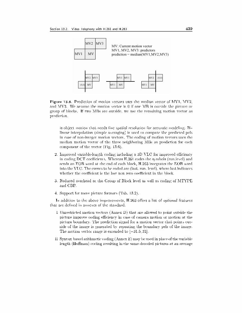
Section 13.2. Video Telephony with H.261 and H.263 439
Figure 13.6. Prediction of motion vectors uses the median vector of MV1, MV2,
and MV3. We assume the motion vector is 0 if one MB is outside the picture or
group of blocks. If two MBs are outside, we use the remaining motion vector as
prediction.
is object motion that needs �ne spatial resolution for accurate modeling. Bi-
linear interpolation (simple averaging) is used to compute the predicted pels
in case of non-integer motion vectors. The coding of motion vectors uses the
median motion vector of the three neighboring MBs as prediction for each
component of the vector (Fig. 13.6).
2. Improved variable-length coding including a 3D VLC for improved eÆciency
in coding DCT coeÆcients. Whereas H.261 codes the symbols (run,level) and
sends an EOB word at the end of each block, H.263 integrates the EOB word
into the VLC. The events to be coded are (last, run, level), where last indicates
whether the coeÆcient is the last non-zero coeÆcient in the block.
3. Reduced overhead at the Group of Block level as well as coding of MTYPE
and CBP.
4. Support for more picture formats (Tab. 13.2).
In addition to the above improvements, H.263 o�ers a list of optional features
that are de�ned in annexes of the standard.
I Unrestricted motion vectors (Annex D) that are allowed to point outside the
picture improve coding eÆciency in case of camera motion or motion at the
picture boundary. The prediction signal for a motion vector that points out-
side of the image is generated by repeating the boundary pels of the image.
The motion vector range is extended to [�31:5; 31].
II Syntax-based arithmetic coding (Annex E) may be used in place of the variable
length (Hu�man) coding resulting in the same decoded pictures at an average
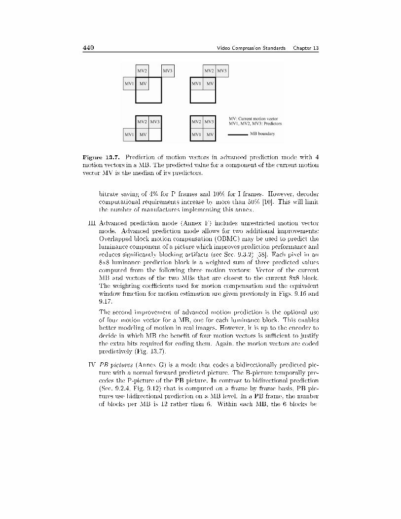
440 Video Compression Standards Chapter 13
Figure 13.7. Prediction of motion vectors in advanced prediction mode with 4
motion vectors in a MB. The predicted value for a component of the current motion
vector MV is the median of its predictors.
bitrate saving of 4% for P frames and 10% for I frames. However, decoder
computational requirements increase by more than 50% [10]. This will limit
the number of manufactures implementing this annex.
III Advanced prediction mode (Annex F) includes unrestricted motion vector
mode. Advanced prediction mode allows for two additional improvements:
Overlapped block motion compensation (OBMC) may be used to predict the
luminance component of a picture which improves prediction performance and
reduces signi�cantly blocking artifacts (see Sec. 9.3.2) [58]. Each pixel in an
8x8 luminance prediction block is a weighted sum of three predicted values
computed from the following three motion vectors: Vector of the current
MB and vectors of the two MBs that are closest to the current 8x8 block.
The weighting coeÆcients used for motion compensation and the equivalent
window function for motion estimation are given previously in Figs. 9.16 and
9.17.
The second improvement of advanced motion prediction is the optional use
of four motion vector for a MB, one for each luminance block. This enables
better modeling of motion in real images. However, it is up to the encoder to
decide in which MB the bene�t of four motion vectors is suÆcient to justify
the extra bits required for coding them. Again, the motion vectors are coded
predictively (Fig. 13.7).
IV PB pictures (Annex G) is a mode that codes a bidirectionally predicted pic-
ture with a normal forward predicted picture. The B-picture temporally pre-
cedes the P-picture of the PB picture. In contrast to bidirectional prediction
(Sec. 9.2.4, Fig. 9.12) that is computed on a frame by frame basis, PB pic-
tures use bidirectional prediction on a MB level. In a PB frame, the number
of blocks per MB is 12 rather than 6. Within each MB, the 6 blocks be-
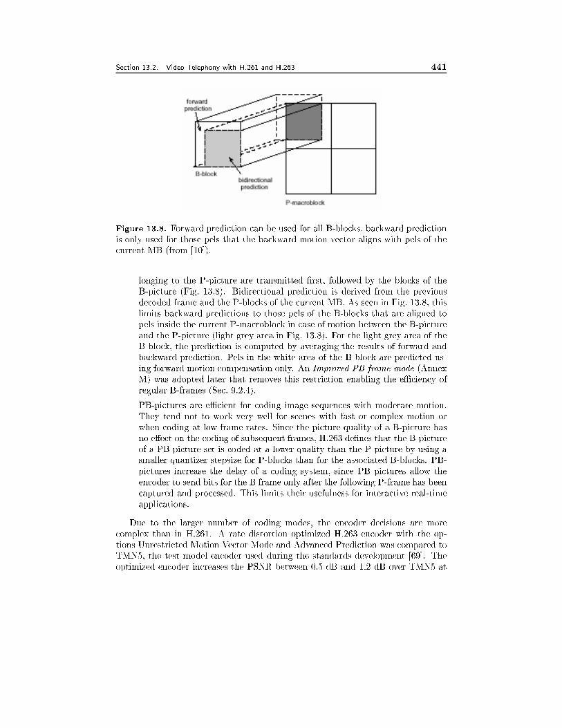
Section 13.2. Video Telephony with H.261 and H.263 441
Figure 13.8. Forward prediction can be used for all B-blocks, backward prediction
is only used for those pels that the backward motion vector aligns with pels of the
current MB (from [10]).
longing to the P-picture are transmitted �rst, followed by the blocks of the
B-picture (Fig. 13.8). Bidirectional prediction is derived from the previous
decoded frame and the P-blocks of the current MB. As seen in Fig. 13.8, this
limits backward predictions to those pels of the B-blocks that are aligned to
pels inside the current P-macroblock in case of motion between the B-picture
and the P-picture (light grey area in Fig. 13.8). For the light grey area of the
B-block, the prediction is computed by averaging the results of forward and
backward prediction. Pels in the white area of the B-block are predicted us-
ing forward motion compensation only. An Improved PB-frame mode (Annex
M) was adopted later that removes this restriction enabling the eÆciency of
regular B-frames (Sec. 9.2.4).
PB-pictures are eÆcient for coding image sequences with moderate motion.
They tend not to work very well for scenes with fast or complex motion or
when coding at low frame rates. Since the picture quality of a B-picture has
no e�ect on the coding of subsequent frames, H.263 de�nes that the B-picture
of a PB-picture set is coded at a lower quality than the P-picture by using a
smaller quantizer stepsize for P-blocks than for the associated B-blocks. PB-
pictures increase the delay of a coding system, since PB pictures allow the
encoder to send bits for the B frame only after the following P-frame has been
captured and processed. This limits their usefulness for interactive real-time
applications.
Due to the larger number of coding modes, the encoder decisions are more
complex than in H.261. A rate distortion optimized H.263 encoder with the op-
tions Unrestricted Motion Vector Mode and Advanced Prediction was compared to
TMN5, the test model encoder used during the standards development [69]. The
optimized encoder increases the PSNR between 0.5 dB and 1.2 dB over TMN5 at
442 Video Compression Standards Chapter 13
bitrates between 20 and 70 kbit/s.
H.263 as of 2000
After the initial version of H.263 was approved, work continued with further op-
tional modes being added. However, since these more than 15 modes are optional,
it is questionable that any manufacturer will implement all these options. ITU
recognized that and added recommendations for preferred modes to the standard.
The most important preferred modes not mentioned above are listed here.
1. Advanced Intra Coding (Annex I): Intra blocks are coded using the block to
the left or above as a prediction provided that block is also coded in intra-
mode. This mode increases coding eÆciency by 10% to 15% for I pictures.
2. Deblocking �lter (Annex J): An adaptive �lter is applied across the boundaries
of decoded 8x8 blocks to reduce blocking artifacts. This �lter a�ects also the
predicted image and is implemented inside the prediction loop of coder and
decoder.
3. Supplemental Enhancement Information (Annex L): This information may
be used to provide tagging information for external use as de�ned by an
application using H.263. Furthermore, this information can be used to signal
enhanced display capabilities like frame freeze, zoom or chroma-keying (see
Sec. 10.3).
4. Improved PB-frame Mode (Annex M): As mentioned before, this mode re-
moves the restrictions placed on the backward prediction of Annex G. There-
fore, this mode enables regular bidirectional prediction (Sec. 9.2.4).
The above tools are developed for enhancing the coding eÆciency. In order to
enable transport of H.263 video over unreliable networks such as wireless networks
and the Internet, a set of tools are also developed for the purpose of error resilience.
These are included in Annex H: Forward Error Correction Using BCH Code, An-
nex K: Flexible Synchronization Marker Insertion Using the Slice Structured Mode,
Annex N and U: Reference Picture Selection, Annex O: Scalability, Annex R: In-
dependent Segment Decoding, Annex V: Data Partitioning and RVLC, Annex W:
Header Repetition. These tools are described in Sec. 14.7.1. Further discussion of
H.263 can be found in [6] and in the standard itself [49].
13.2.3 Comparison
Fig. 13.9 compares the performance of H.261 and H.263 [10]. H.261 is shown with
and without using the �lter in the loop (Curves 3 and 5). Since H.261 was designed
for data rates of 64 kbit/s and up, we discuss Fig. 13.9 at this rate. Without options,
H.263 outperform H.261 by 2 dB (Curves 2 and 3). Another dB is gained if we use
the options advanced prediction, syntax-based arithmetic coding, and PB frames
(Curve 1). Curve 4 shows that restricting motion vectors in H.263 to integer-pel
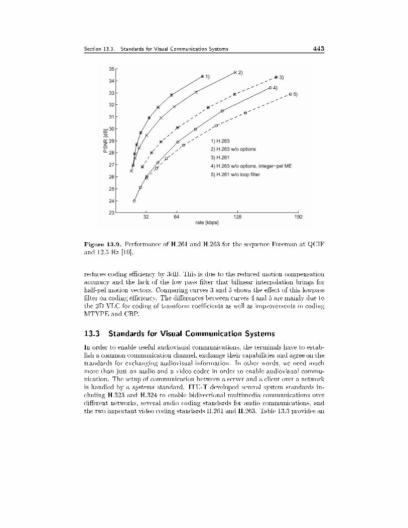
Section 13.3. Standards for Visual Communication Systems 443
Figure 13.9. Performance of H.261 and H.263 for the sequence Foreman at QCIF
and 12.5 Hz [10].
reduces coding eÆciency by 3dB. This is due to the reduced motion compensation
accuracy and the lack of the low pass �lter that bilinear interpolation brings for
half-pel motion vectors. Comparing curves 3 and 5 shows the e�ect of this lowpass
�lter on coding eÆciency. The di�erences between curves 4 and 5 are mainly due to
the 3D VLC for coding of transform coeÆcients as well as improvements in coding
MTYPE and CBP.
13.3 Standards for Visual Communication Systems
In order to enable useful audiovisual communications, the terminals have to estab-
lish a common communication channel, exchange their capabilities and agree on the
standards for exchanging audiovisual information. In other words, we need much
more than just an audio and a video codec in order to enable audiovisual commu-
nication. The setup of communication between a server and a client over a network
is handled by a systems standard. ITU-T developed several system standards in-
cluding H.323 and H.324 to enable bidirectional multimedia communications over
di�erent networks, several audio coding standards for audio communications, and
the two important video coding standards H.261 and H.263. Table 13.3 provides an
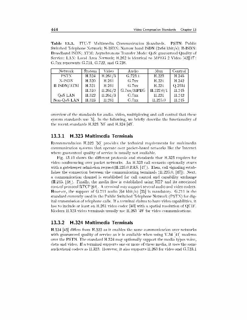
444 Video Compression Standards Chapter 13
Table 13.3. ITU-T Multimedia Communication Standards. PSTN: Public
Switched Telephone Network; N-ISDN: Narrow band ISDN (2x64 kbit/s); B-ISDN:
Broadband ISDN; ATM: Asynchronous Transfer Mode; QoS: guaranteed Quality of
Service; LAN: Local Area Network; H.262 is identical to MPEG-2 Video [42][17];
G.7xx represents G.711, G.722, and G.728.
Network System Video Audio Mux Control
PSTN H.324 H.261/3 G.723.1 H.223 H.245
N-ISDN H.320 H.261 G.7xx H.221 H.242
B-ISDN/ATM H.321 H.261 G.7xx H.221 Q.2931
H.310 H.261/2 G.7xx/MPEG H.222.0/1 H.245
QoS LAN H.322 H.261/3 G.7xx H.221 H.242
Non-QoS LAN H.323 H.261 G.7xx H.225.0 H.245
overview of the standards for audio, video, multiplexing and call control that these
system standards use [5]. In the following, we brie y describe the functionality of
the recent standards H.323 [50] and H.324 [43].
13.3.1 H.323 Multimedia Terminals
Recommendation H.323 [50] provides the technical requirements for multimedia
communication systems that operate over packet-based networks like the Internet
where guaranteed quality of service is usually not available.
Fig. 13.10 shows the di�erent protocols and standards that H.323 requires for
video conferencing over packet networks. An H.323 call scenario optionally starts
with a gatekeeper admission request(H.225.0 RAS, [47]). Then, call signaling estab-
lishes the connection between the communicating terminals (H.225.0, [47]). Next,
a communication channel is established for call control and capability exchange
(H.245, [48]). Finally, the media ow is established using RTP and its associated
control protocol RTCP [64]. A terminal may support several audio and video codecs.
However, the support of G.711 audio (64 kbit/s) [35] is mandatory. G.711 is the
standard currently used in the Public Switched Telephone Network (PSTN) for dig-
ital transmission of telephone calls. If a terminal claims to have video capabilities, it
has to include at least an H.261 video codec [40] with a spatial resolution of QCIF.
Modern H.323 video terminals usually use H.263 [49] for video communications.
13.3.2 H.324 Multimedia Terminals
H.324 [43] di�ers from H.323 as it enables the same communication over networks
with guaranteed quality of service as it is available when using V.34 [41] modems
over the PSTN. The standard H.324 may optionally support the media types voice,
data and video. If a terminal supports one or more of these media, it uses the same
audiovisual codecs as H.323. However, it also supports H.263 for video and G.723.1
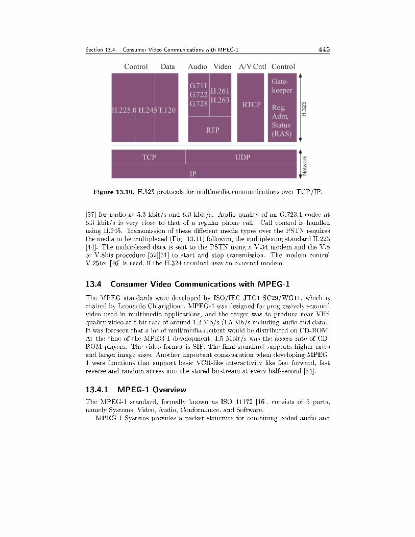
Section 13.4. Consumer Video Communications with MPEG-1 445
H.225.0 H.245
G.711
G.722
G.728
H.261
H.263
RTP
RTCP
Gate-
keeper
Reg,
Adm,
Status
(RAS)
Control Data Audio Video A/V Cntl Control
TCP UDP
IP
T.120
Netw
ork
H.3
23
Figure 13.10. H.323 protocols for multimedia communications over TCP/IP.
[37] for audio at 5.3 kbit/s and 6.3 kbit/s. Audio quality of an G.723.1 codec at
6.3 kbit/s is very close to that of a regular phone call. Call control is handled
using H.245. Transmission of these di�erent media types over the PSTN requires
the media to be multiplexed (Fig. 13.11) following the multiplexing standard H.223
[44]. The multiplexed data is sent to the PSTN using a V.34 modem and the V.8
or V.8bis procedure [52][51] to start and stop transmission. The modem control
V.25ter [46] is used, if the H.324 terminal uses an external modem.
13.4 Consumer Video Communications with MPEG-1
The MPEG standards were developed by ISO/IEC JTC1 SC29/WG11, which is
chaired by Leonardo Chiariglione. MPEG-1 was designed for progressively scanned
video used in multimedia applications, and the target was to produce near VHS
quality video at a bit rate of around 1.2 Mb/s (1.5 Mb/s including audio and data).
It was foreseen that a lot of multimedia content would be distributed on CD-ROM.
At the time of the MPEG-1 development, 1.5 Mbit/s was the access rate of CD-
ROM players. The video format is SIF. The �nal standard supports higher rates
and larger image sizes. Another important consideration when developing MPEG-
1 were functions that support basic VCR-like interactivity like fast forward, fast
reverse and random access into the stored bitstream at every half-second [54].
13.4.1 MPEG-1 Overview
The MPEG-1 standard, formally known as ISO 11172 [16], consists of 5 parts,
namely Systems, Video, Audio, Conformance, and Software.
MPEG-1 Systems provides a packet structure for combining coded audio and
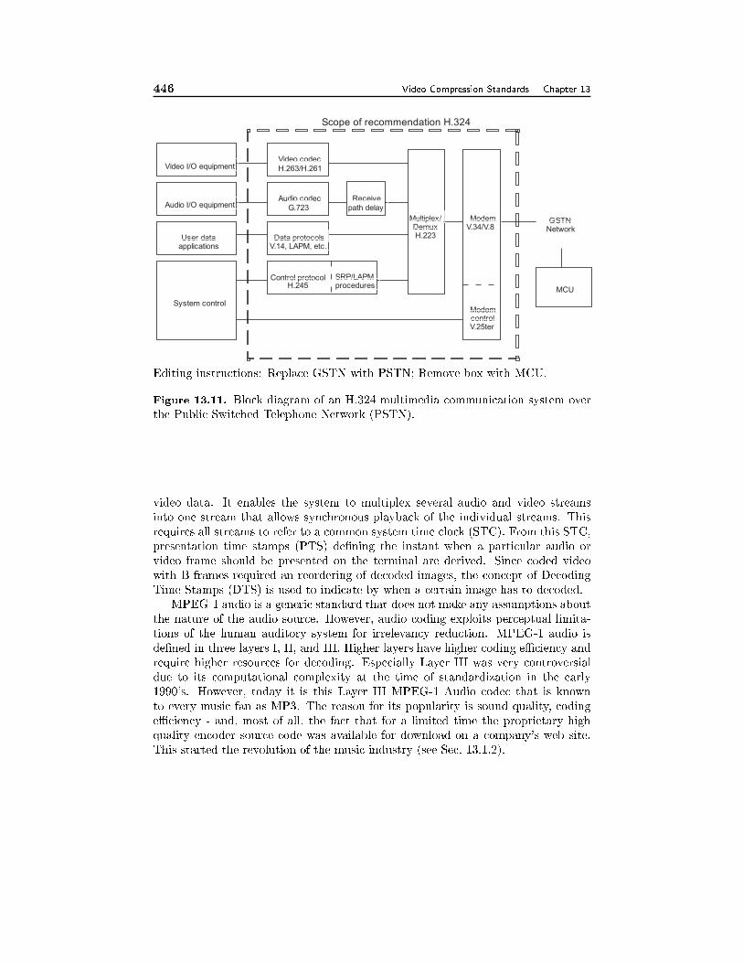
446 Video Compression Standards Chapter 13
Scope of recommendation H.324
System control
User dataapplications
Audio I/O equipment
Video I/O equipmentVideo codec
H.263/H.261
Audio codec
G.723
Data protocolsV.14, LAPM, etc.
Receive
path delay
Multiplex/DemuxH.223
ModemV.34/V.8
ModemcontrolV.25ter
GSTNNetwork
MCU
SRP/LAPMprocedures
Control protocolH.245
Editing instructions: Replace GSTN with PSTN; Remove box with MCU.
Figure 13.11. Block diagram of an H.324 multimedia communication system over
the Public Switched Telephone Network (PSTN).
video data. It enables the system to multiplex several audio and video streams
into one stream that allows synchronous playback of the individual streams. This
requires all streams to refer to a common system time clock (STC). From this STC,
presentation time stamps (PTS) de�ning the instant when a particular audio or
video frame should be presented on the terminal are derived. Since coded video
with B-frames required an reordering of decoded images, the concept of Decoding
Time Stamps (DTS) is used to indicate by when a certain image has to decoded.
MPEG-1 audio is a generic standard that does not make any assumptions about
the nature of the audio source. However, audio coding exploits perceptual limita-
tions of the human auditory system for irrelevancy reduction. MPEG-1 audio is
de�ned in three layers I, II, and III. Higher layers have higher coding eÆciency and
require higher resources for decoding. Especially Layer III was very controversial
due to its computational complexity at the time of standardization in the early
1990's. However, today it is this Layer III MPEG-1 Audio codec that is known
to every music fan as MP3. The reason for its popularity is sound quality, coding
eÆciency - and, most of all, the fact that for a limited time the proprietary high
quality encoder source code was available for download on a company's web site.
This started the revolution of the music industry (see Sec. 13.1.2).
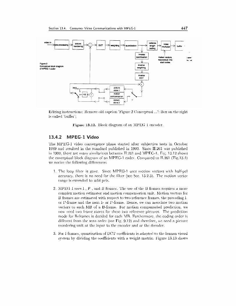
Section 13.4. Consumer Video Communications with MPEG-1 447
Editing instructions: Remove old caption 'Figure 2 Conceptual ...'; Box on the right
is called 'bu�er';
Figure 13.12. Block diagram of an MPEG-1 encoder.
13.4.2 MPEG-1 Video
The MPEG-1 video convergence phase started after subjective tests in October
1989 and resulted in the standard published in 1993. Since H.261 was published
in 1990, there are many similarities between H.261 and MPEG-1. Fig. 13.12 shows
the conceptual block diagram of an MPEG-1 coder. Compared to H.261 (Fig.13.4)
we notice the following di�erences:
1. The loop �lter is gone. Since MPEG-1 uses motion vectors with half-pel
accuracy, there is no need for the �lter (see Sec. 13.2.3). The motion vector
range is extended to �64 pels.
2. MPEG-1 uses I-, P-, and B-frames. The use of the B-frames requires a more
complex motion estimator and motion compensation unit. Motion vectors for
B-frames are estimated with respect to two reference frames, the preceding I-
or P-frame and the next I- or P-frame. Hence, we can associate two motion
vectors to each MB of a B-frame. For motion compensated prediction, we
now need two frame stores for these two reference pictures. The prediction
mode for B-frames is decided for each MB. Furthermore, the coding order is
di�erent from the scan order (see Fig. 9.12) and therefore, we need a picture
reordering unit at the input to the encoder and at the decoder.
3. For I-frames, quantization of DCT coeÆcients is adapted to the human visual
system by dividing the coeÆcients with a weight matrix. Figure 13.13 shows
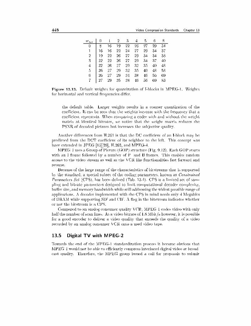
448 Video Compression Standards Chapter 13
wu;v 0 1 2 3 4 5 6 8
0 8 16 19 22 26 27 29 34
1 16 16 22 24 27 29 34 37
2 19 22 26 27 29 34 34 38
3 22 22 26 27 29 34 37 40
4 22 26 27 29 32 35 40 48
5 26 27 29 32 35 40 48 58
6 26 27 29 34 38 46 56 69
7 27 29 35 38 46 56 69 83
Figure 13.13. Default weights for quantization of I-blocks in MPEG-1. Weights
for horizontal and vertical frequencies di�er.
the default table. Larger weights results in a coarser quantization of the
coeÆcient. It can be seen that the weights increase with the frequency that a
coeÆcient represents. When comparing a coder with and without the weight
matrix at identical bitrates, we notice that the weight matrix reduces the
PSNR of decoded pictures but increases the subjective quality.
Another di�erences from H.261 is that the DC coeÆcient of an I-block may be
predicted from the DCT coeÆcient of its neighbor to the left. This concept was
later extended in JPEG [15][39], H.263, and MPEG-4.
MPEG-1 uses a Group of Picture (GOP) structure (Fig. 9.12). Each GOP starts
with an I frame followed by a number of P- and B-frames. This enables random
access to the video stream as well as the VCR like functionalities fast forward and
reverse.
Because of the large range of the characteristics of bitstreams that is supported
by the standard, a special subset of the coding parameters, known as Constrained
Parameters Set (CPS), has been de�ned (Tab. 13.4). CPS is a limited set of sam-
pling and bitrate parameters designed to limit computational decoder complexity,
bu�er size, and memory bandwidth while still addressing the widest possible range of
applications. A decoder implemented with the CPS in mind needs only 4 Megabits
of DRAM while supporting SIF and CIF. A ag in the bitstream indicates whether
or not the bitstream is a CPS.
Compared to an analog consumer quality VCR, MPEG-1 codes video with only
half the number of scan lines. At a video bitrate of 1.8 Mbit/s however, it is possible
for a good encoder to deliver a video quality that exceeds the quality of a video
recorded by an analog consumer VCR onto a used video tape.
13.5 Digital TV with MPEG-2
Towards the end of the MPEG-1 standardization process it became obvious that
MPEG-1 would not be able to eÆciently compress interlaced digital video at broad-
cast quality. Therefore, the MPEG group issued a call for proposals to submit
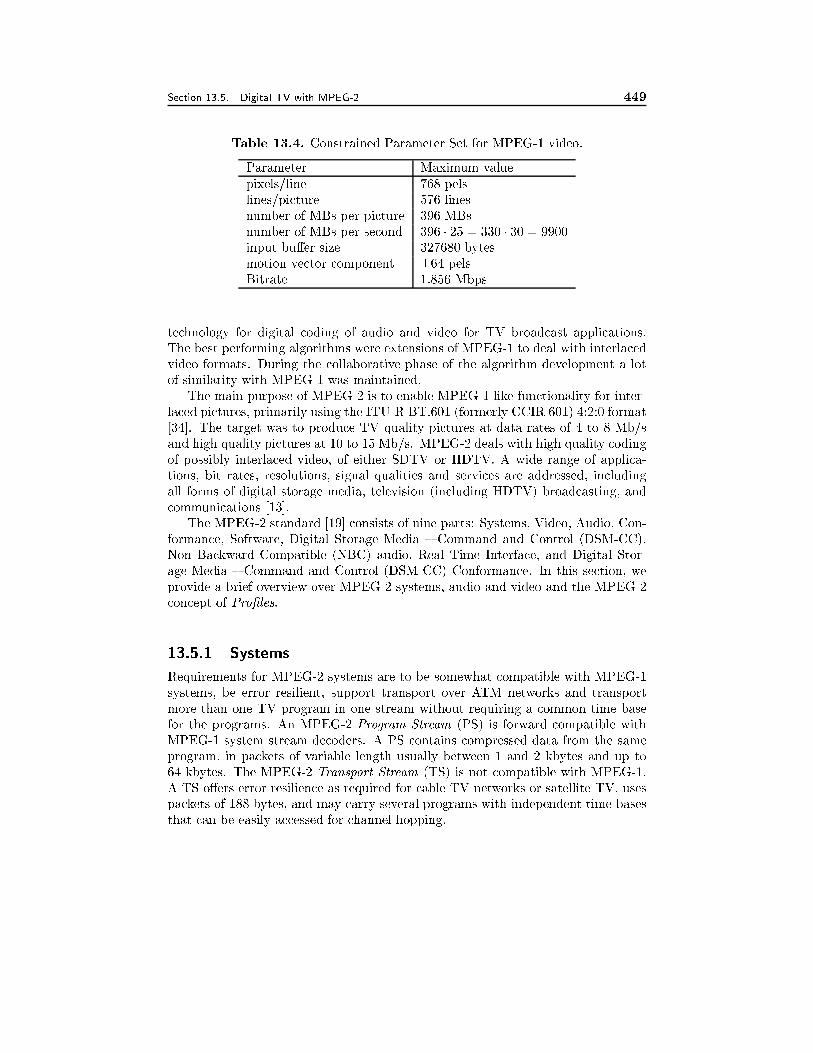
Section 13.5. Digital TV with MPEG-2 449
Table 13.4. Constrained Parameter Set for MPEG-1 video.
Parameter Maximum value
pixels/line 768 pels
lines/picture 576 lines
number of MBs per picture 396 MBs
number of MBs per second 396 � 25 = 330 � 30 = 9900
input bu�er size 327680 bytes
motion vector component �64 pelsBitrate 1.856 Mbps
technology for digital coding of audio and video for TV broadcast applications.
The best performing algorithms were extensions of MPEG-1 to deal with interlaced
video formats. During the collaborative phase of the algorithm development a lot
of similarity with MPEG-1 was maintained.
The main purpose of MPEG-2 is to enable MPEG-1 like functionality for inter-
laced pictures, primarily using the ITU-R BT.601 (formerly CCIR 601) 4:2:0 format
[34]. The target was to produce TV quality pictures at data rates of 4 to 8 Mb/s
and high quality pictures at 10 to 15 Mb/s. MPEG-2 deals with high quality coding
of possibly interlaced video, of either SDTV or HDTV. A wide range of applica-
tions, bit rates, resolutions, signal qualities and services are addressed, including
all forms of digital storage media, television (including HDTV) broadcasting, and
communications [13].
The MPEG-2 standard [19] consists of nine parts: Systems, Video, Audio, Con-
formance, Software, Digital Storage Media { Command and Control (DSM-CC),
Non Backward Compatible (NBC) audio, Real Time Interface, and Digital Stor-
age Media { Command and Control (DSM-CC) Conformance. In this section, we
provide a brief overview over MPEG-2 systems, audio and video and the MPEG-2
concept of Pro�les.
13.5.1 Systems
Requirements for MPEG-2 systems are to be somewhat compatible with MPEG-1
systems, be error resilient, support transport over ATM networks and transport
more than one TV program in one stream without requiring a common time base
for the programs. An MPEG-2 Program Stream (PS) is forward compatible with
MPEG-1 system stream decoders. A PS contains compressed data from the same
program, in packets of variable length usually between 1 and 2 kbytes and up to
64 kbytes. The MPEG-2 Transport Stream (TS) is not compatible with MPEG-1.
A TS o�ers error resilience as required for cable TV networks or satellite TV, uses
packets of 188 bytes, and may carry several programs with independent time bases
that can be easily accessed for channel hopping.
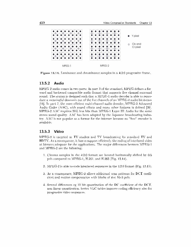
450 Video Compression Standards Chapter 13
MPEG-1 MPEG-2
Y pixel
Cb and
Cr pixel
Figure 13.14. Luminance and chrominance samples in a 4:2:0 progressive frame.
13.5.2 Audio
MPEG-2 audio comes in two parts: In part 3 of the standard, MPEG de�nes a for-
ward and backward compatible audio format that supports �ve channel surround
sound. The syntax is designed such that a MPEG-1 audio decoder is able to repro-
duce a meaningful downmix out of the �ve channels of an MPEG-2 audio bitstream
[18]. In part 7, the more eÆcient multi-channel audio decoder, MPEG-2 Advanced
Audio Coder (AAC), with sound e�ects and many other features is de�ned [20].
MPEG-2 AAC requires 30% less bits than MPEG-1 Layer III Audio for the same
stereo sound quality. AAC has been adopted by the Japanese broadcasting indus-
try. AAC is not popular as a format for the internet because no "free" encoder is
available.
13.5.3 Video
MPEG-2 is targeted at TV studios and TV broadcasting for standard TV and
HDTV. As a consequence, it has to support eÆciently the coding of interlaced video
at bitrates adequate for the applications. The major di�erences between MPEG-1
and MPEG-2 are the following:
1. Chroma samples in the 4:2:0 format are located horizontally shifted by 0.5
pels compared to MPEG-1, H.261, and H.263 (Fig. 13.14).
2. MPEG-2 is able to code interlaced sequences in the 4:2:0 format (Fig. 13.15).
3. As a consequence, MPEG-2 allows additional scan patterns for DCT coeÆ-
cient and motion compensation with blocks of size 16x8 pels.
4. Several di�erences eg 10 bit quantization of the DC coeÆcient of the DCT,
non-linear quantization, better VLC tables improve coding eÆciency also for
progressive video sequences.
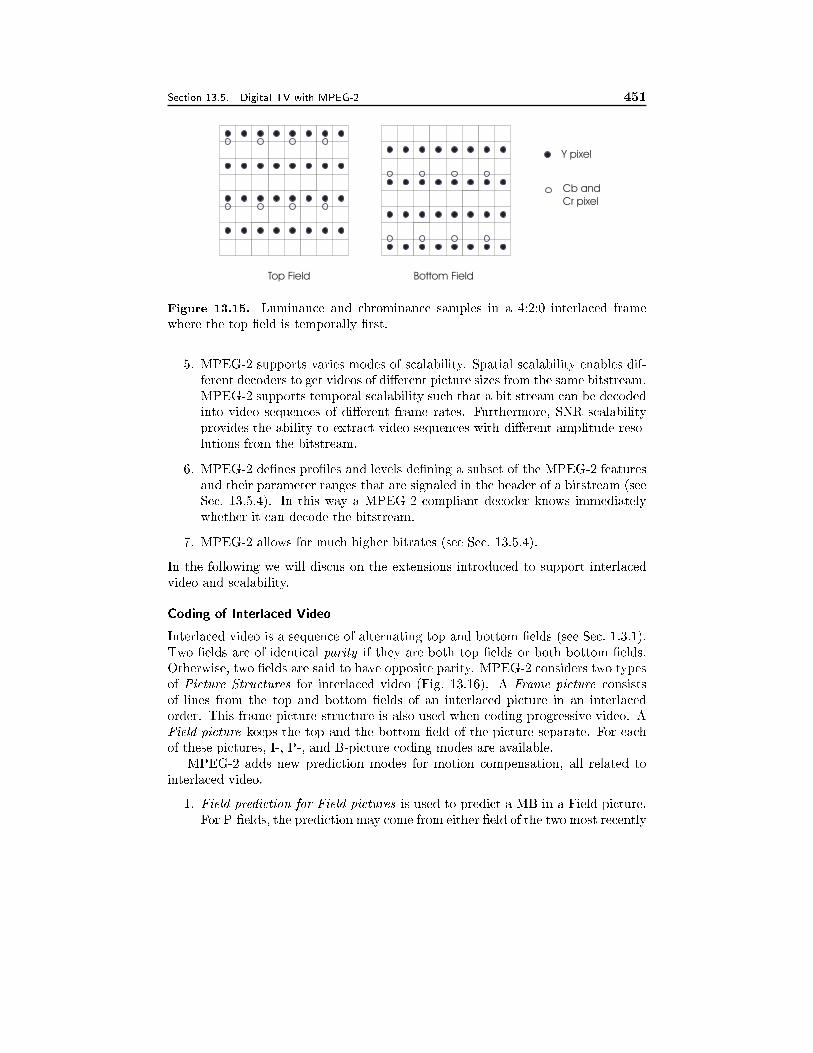
Section 13.5. Digital TV with MPEG-2 451
Y pixel
Cb and
Cr pixel
Top Field Bottom Field
Figure 13.15. Luminance and chrominance samples in a 4:2:0 interlaced frame
where the top �eld is temporally �rst.
5. MPEG-2 supports varies modes of scalability. Spatial scalability enables dif-
ferent decoders to get videos of di�erent picture sizes from the same bitstream.
MPEG-2 supports temporal scalability such that a bit stream can be decoded
into video sequences of di�erent frame rates. Furthermore, SNR scalability
provides the ability to extract video sequences with di�erent amplitude reso-
lutions from the bitstream.
6. MPEG-2 de�nes pro�les and levels de�ning a subset of the MPEG-2 features
and their parameter ranges that are signaled in the header of a bitstream (see
Sec. 13.5.4). In this way a MPEG-2 compliant decoder knows immediately
whether it can decode the bitstream.
7. MPEG-2 allows for much higher bitrates (see Sec. 13.5.4).
In the following we will discus on the extensions introduced to support interlaced
video and scalability.
Coding of Interlaced Video
Interlaced video is a sequence of alternating top and bottom �elds (see Sec. 1.3.1).
Two �elds are of identical parity if they are both top �elds or both bottom �elds.
Otherwise, two �elds are said to have opposite parity. MPEG-2 considers two types
of Picture Structures for interlaced video (Fig. 13.16). A Frame picture consists
of lines from the top and bottom �elds of an interlaced picture in an interlaced
order. This frame picture structure is also used when coding progressive video. A
Field-picture keeps the top and the bottom �eld of the picture separate. For each
of these pictures, I-, P-, and B-picture coding modes are available.
MPEG-2 adds new prediction modes for motion compensation, all related to
interlaced video.
1. Field prediction for Field-pictures is used to predict a MB in a Field-picture.
For P-�elds, the prediction may come from either �eld of the two most recently
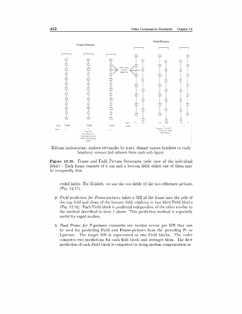
452 Video Compression Standards Chapter 13
Editing instructions: replace rectangles by stars; change square brackets to curly
brackets; remove 3rd column from each sub �gure.
Figure 13.16. Frame and Field Picture Structures (side view of the individual
�elds) : Each frame consists of a top and a bottom �eld, either one of them may
be temporally �rst.
coded �elds. For B-�elds, we use the two �elds of the two reference pictures
(Fig. 13.17).
2. Field prediction for Frame-pictures splits a MB of the frame into the pels of
the top �eld and those of the bottom �eld resulting in two 16x8 Field blocks
(Fig. 13.18). Each Field block is predicted independent of the other similar to
the method described in item 1 above. This prediction method is especially
useful for rapid motion.
3. Dual Prime for P-pictures transmits one motion vector per MB that can
be used for predicting Field and Frame-pictures from the preceding P- or
I-picture. The target MB is represented as two Field blocks. The coder
computes two predictions for each �eld block and averages them. The �rst
prediction of each Field block is computed by doing motion compensation us-
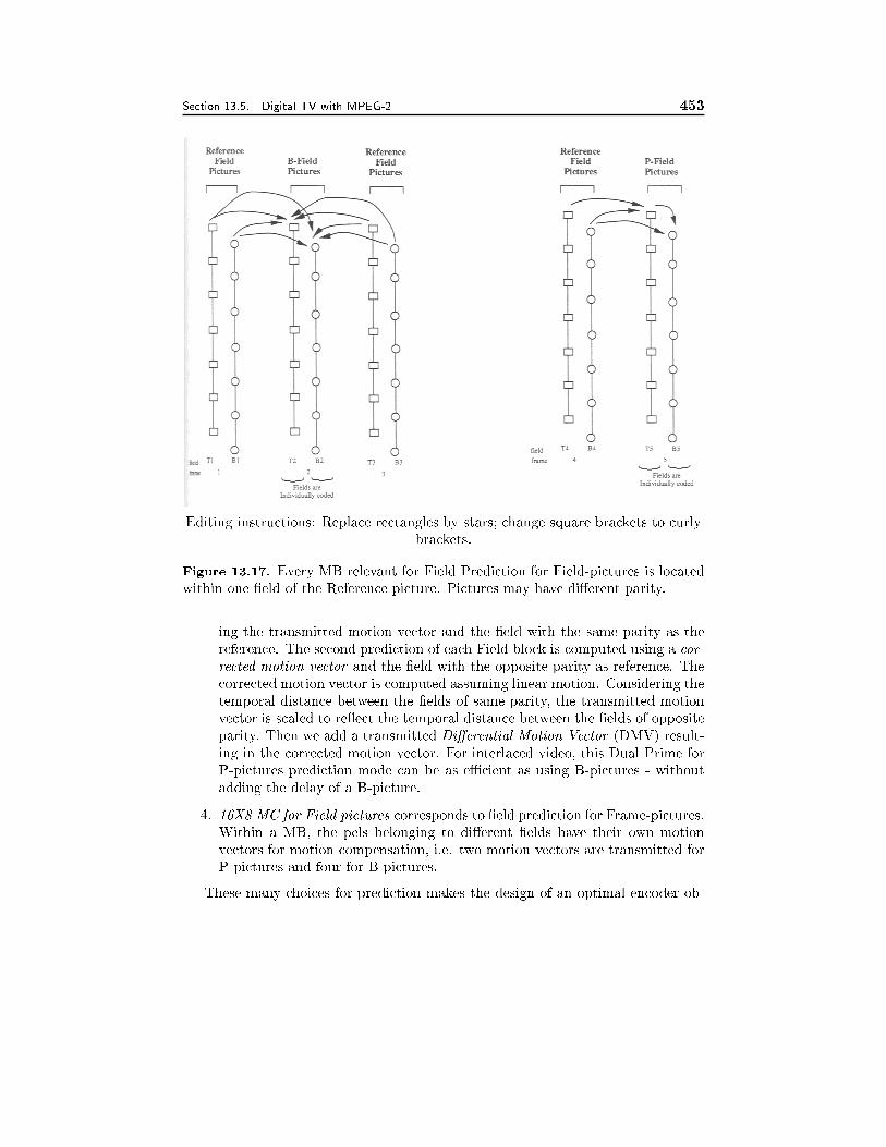
Section 13.5. Digital TV with MPEG-2 453
Editing instructions: Replace rectangles by stars; change square brackets to curly
brackets.
Figure 13.17. Every MB relevant for Field Prediction for Field-pictures is located
within one �eld of the Reference picture. Pictures may have di�erent parity.
ing the transmitted motion vector and the �eld with the same parity as the
reference. The second prediction of each Field block is computed using a cor-
rected motion vector and the �eld with the opposite parity as reference. The
corrected motion vector is computed assuming linear motion. Considering the
temporal distance between the �elds of same parity, the transmitted motion
vector is scaled to re ect the temporal distance between the �elds of opposite
parity. Then we add a transmitted Di�erential Motion Vector (DMV) result-
ing in the corrected motion vector. For interlaced video, this Dual Prime for
P-pictures prediction mode can be as eÆcient as using B-pictures - without
adding the delay of a B-picture.
4. 16X8 MC for Field pictures corresponds to �eld prediction for Frame-pictures.
Within a MB, the pels belonging to di�erent �elds have their own motion
vectors for motion compensation, i.e. two motion vectors are transmitted for
P-pictures and four for B-pictures.
These many choices for prediction makes the design of an optimal encoder ob-
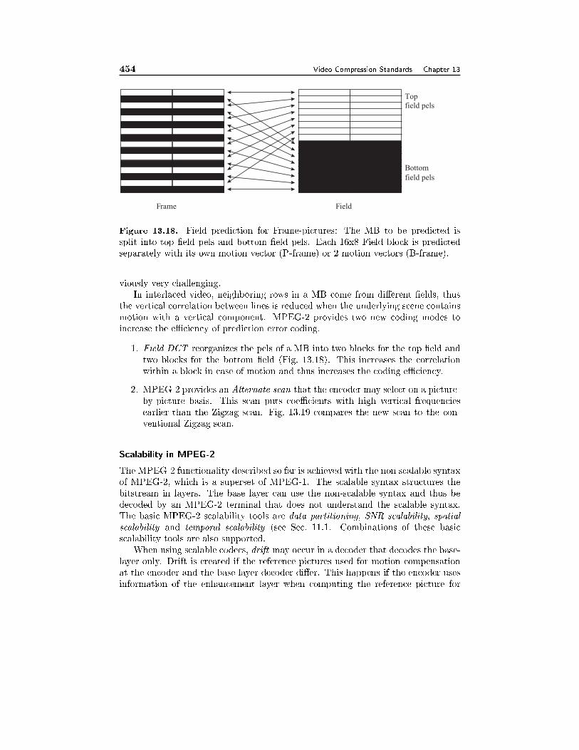
454 Video Compression Standards Chapter 13
Bottom
field pels
Top
field pels
Frame Field
Figure 13.18. Field prediction for Frame-pictures: The MB to be predicted is
split into top �eld pels and bottom �eld pels. Each 16x8 Field block is predicted
separately with its own motion vector (P-frame) or 2 motion vectors (B-frame).
viously very challenging.
In interlaced video, neighboring rows in a MB come from di�erent �elds, thus
the vertical correlation between lines is reduced when the underlying scene contains
motion with a vertical component. MPEG-2 provides two new coding modes to
increase the eÆciency of prediction error coding.
1. Field DCT reorganizes the pels of a MB into two blocks for the top �eld and
two blocks for the bottom �eld (Fig. 13.18). This increases the correlation
within a block in case of motion and thus increases the coding eÆciency.
2. MPEG-2 provides an Alternate scan that the encoder may select on a picture-
by-picture basis. This scan puts coeÆcients with high vertical frequencies
earlier than the Zigzag scan. Fig. 13.19 compares the new scan to the con-
ventional Zigzag scan.
Scalability in MPEG-2
The MPEG-2 functionality described so far is achieved with the non scalable syntax
of MPEG-2, which is a superset of MPEG-1. The scalable syntax structures the
bitstream in layers. The base layer can use the non-scalable syntax and thus be
decoded by an MPEG-2 terminal that does not understand the scalable syntax.
The basic MPEG-2 scalability tools are data partitioning, SNR scalability, spatial
scalability and temporal scalability (see Sec. 11.1. Combinations of these basic
scalability tools are also supported.
When using scalable codecs, drift may occur in a decoder that decodes the base-
layer only. Drift is created if the reference pictures used for motion compensation
at the encoder and the base-layer decoder di�er. This happens if the encoder uses
information of the enhancement layer when computing the reference picture for
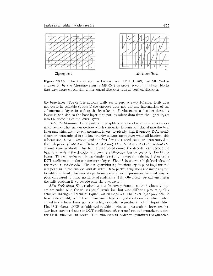
Section 13.5. Digital TV with MPEG-2 455
Zigzag scan Alternate Scan
Figure 13.19. The Zigzag scan as known from H.261, H.263, and MPEG-1 is
augmented by the Alternate scan in MPEG-2 in order to code interlaced blocks
that have more correlation in horizontal direction than in vertical direction.
the base layer. The drift is automatically set to zero at every I-frame. Drift does
not occur in scalable codecs if the encoder does not use any information of the
enhancement layer for coding the base layer. Furthermore, a decoder decoding
layers in addition to the base layer may not introduce data from the upper layers
into the decoding of the lower layers.
Data Partitioning : Data partitioning splits the video bit stream into two or
more layers. The encoder decides which syntactic elements are placed into the base
layer and which into the enhancement layers. Typically, high frequency DCT coeÆ-
cients are transmitted in the low priority enhancement layer while all headers, side
information, motion vectors, and the �rst few DCT coeÆcients are transmitted in
the high priority base layer. Data partitioning is appropriate when two transmission
channels are available. Due to the data partitioning, the decoder can decode the
base layer only if the decoder implements a bitstream loss concealer for the higher
layers. This concealer can be as simple as setting to zero the missing higher order
DCT coeÆcients in the enhancement layer. Fig. 13.20 shows a high-level view of
the encoder and decoder. The data partitioning functionality may be implemented
independent of the encoder and decoder. Data partitioning does not incur any no-
ticeable overhead. However, its performance in an error-prone environment may be
poor compared to other methods of scalability [13]. Obviously, we will encounter
the drift problem if we decode only the base layer.
SNR Scalability : SNR scalability is a frequency domain method where all lay-
ers are coded with the same spatial resolution, but with di�ering picture quality
achieved through di�erent MB quantization stepsizes. The lower layer provides the
basic video quality while the enhancement layer carry the information which, when
added to the lower layer, generate a higher quality reproduction of the input video.
Fig. 13.21 shows a SNR scalable coder, which includes a non-scalable base encoder.
The base encoder feeds the DCT coeÆcients after transform and quantization into
the SNR enhancement coder. The enhancement coder re-quantizes the quantiza-
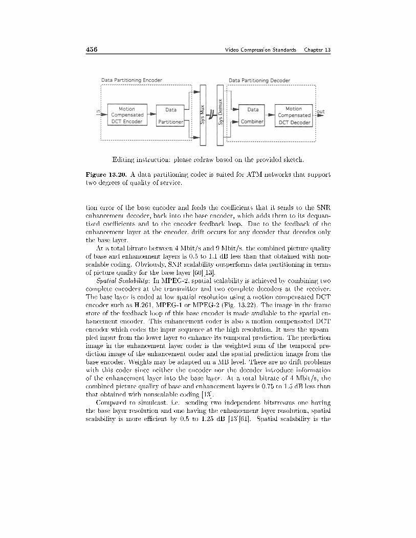
456 Video Compression Standards Chapter 13
Editing instruction: please redraw based on the provided sketch.
Figure 13.20. A data partitioning codec is suited for ATM networks that support
two degrees of quality of service.
tion error of the base encoder and feeds the coeÆcients that it sends to the SNR
enhancement decoder, back into the base encoder, which adds them to its dequan-
tized coeÆcients and to the encoder feedback loop. Due to the feedback of the
enhancement layer at the encoder, drift occurs for any decoder that decodes only
the base layer.
At a total bitrate between 4 Mbit/s and 9 Mbit/s, the combined picture quality
of base and enhancement layers is 0.5 to 1.1 dB less than that obtained with non-
scalable coding. Obviously, SNR scalability outperforms data partitioning in terms
of picture quality for the base layer [60][13].
Spatial Scalability : In MPEG-2, spatial scalability is achieved by combining two
complete encoders at the transmitter and two complete decoders at the receiver.
The base layer is coded at low spatial resolution using a motion compensated DCT
encoder such as H.261, MPEG-1 or MPEG-2 (Fig. 13.22). The image in the frame
store of the feedback loop of this base encoder is made available to the spatial en-
hancement encoder. This enhancement coder is also a motion compensated DCT
encoder which codes the input sequence at the high resolution. It uses the upsam-
pled input from the lower layer to enhance its temporal prediction. The prediction
image in the enhancement layer coder is the weighted sum of the temporal pre-
diction image of the enhancement coder and the spatial prediction image from the
base encoder. Weights may be adapted on a MB level. There are no drift problems
with this coder since neither the encoder nor the decoder introduce information
of the enhancement layer into the base layer. At a total bitrate of 4 Mbit/s, the
combined picture quality of base and enhancement layers is 0.75 to 1.5 dB less than
that obtained with nonscalable coding [13].
Compared to simulcast, i.e. sending two independent bitstreams one having
the base layer resolution and one having the enhancement layer resolution, spatial
scalability is more eÆcient by 0.5 to 1.25 dB [13][61]. Spatial scalability is the
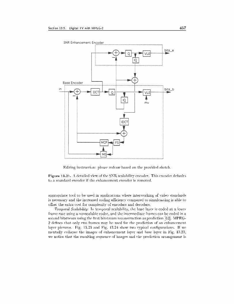
Section 13.5. Digital TV with MPEG-2 457
Editing instruction: please redraw based on the provided sketch.
Figure 13.21. A detailed view of the SNR scalability encoder. This encoder defaults
to a standard encoder if the enhancement encoder is removed.
appropriate tool to be used in applications where interworking of video standards
is necessary and the increased coding eÆciency compared to simulcasting is able to
o�set the extra cost for complexity of encoders and decoders.
Temporal Scalability : In temporal scalability, the base layer is coded at a lower
frame rate using a nonscalable codec, and the intermediate frames can be coded in a
second bitstream using the �rst bitstream reconstruction as prediction [62]. MPEG-
2 de�nes that only two frames may be used for the prediction of an enhancement
layer pictures. Fig. 13.23 and Fig. 13.24 show two typical con�gurations. If we
mentally collapse the images of enhancement layer and base layer in Fig. 13.23,
we notice that the resulting sequence of images and the prediction arrangement is
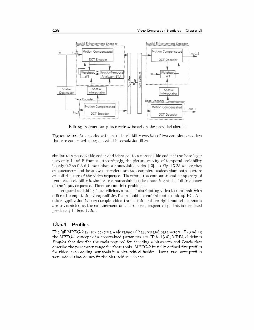
458 Video Compression Standards Chapter 13
Editing instruction: please redraw based on the provided sketch.
Figure 13.22. An encoder with spatial scalability consists of two complete encoders
that are connected using a spatial interpolation �lter.
similar to a nonscalable coder and identical to a nonscalable coder if the base layer
uses only I and P frames. Accordingly, the picture quality of temporal scalability
is only 0.2 to 0.3 dB lower than a nonscalable coder [13]. In Fig. 13.25 we see that
enhancement and base layer encoders are two complete codecs that both operate
at half the rate of the video sequence. Therefore, the computational complexity of
temporal scalability is similar to a nonscalable coder operating at the full frequency
of the input sequence. There are no drift problems.
Temporal scalability is an eÆcient means of distributing video to terminals with
di�erent computational capabilities like a mobile terminal and a desktop PC. An-
other application is stereoscopic video transmission where right and left channels
are transmitted as the enhancement and base layer, respectively. This is discussed
previously in Sec. 12.5.1.
13.5.4 Pro�les
The full MPEG-2 syntax covers a wide range of features and parameters. Extending
the MPEG-1 concept of a constrained parameter set (Tab. 13.4), MPEG-2 de�nes
Pro�les that describe the tools required for decoding a bitstream and Levels that
describe the parameter range for these tools. MPEG-2 initially de�ned �ve pro�les
for video, each adding new tools in a hierarchical fashion. Later, two more pro�les
were added that do not �t the hierarchical scheme:
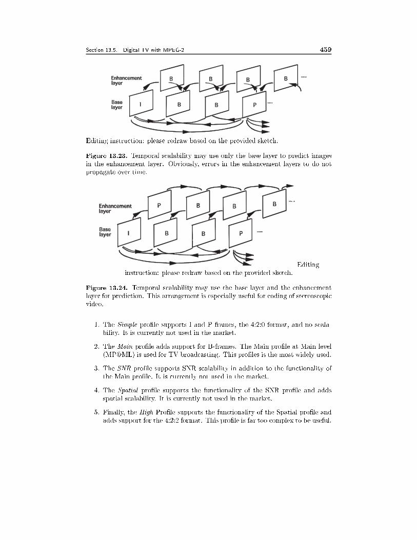
Section 13.5. Digital TV with MPEG-2 459
Editing instruction: please redraw based on the provided sketch.
Figure 13.23. Temporal scalability may use only the base layer to predict images
in the enhancement layer. Obviously, errors in the enhancement layers to do not
propagate over time.
Editing
instruction: please redraw based on the provided sketch.
Figure 13.24. Temporal scalability may use the base layer and the enhancement
layer for prediction. This arrangement is especially useful for coding of stereoscopic
video.
1. The Simple pro�le supports I and P frames, the 4:2:0 format, and no scala-
bility. It is currently not used in the market.
2. The Main pro�le adds support for B-frames. The Main pro�le at Main level
(MP@ML) is used for TV broadcasting. This pro�les is the most widely used.
3. The SNR pro�le supports SNR scalability in addition to the functionality of
the Main pro�le. It is currently not used in the market.
4. The Spatial pro�le supports the functionality of the SNR pro�le and adds
spatial scalability. It is currently not used in the market.
5. Finally, the High Pro�le supports the functionality of the Spatial pro�le and
adds support for the 4:2:2 format. This pro�le is far too complex to be useful.
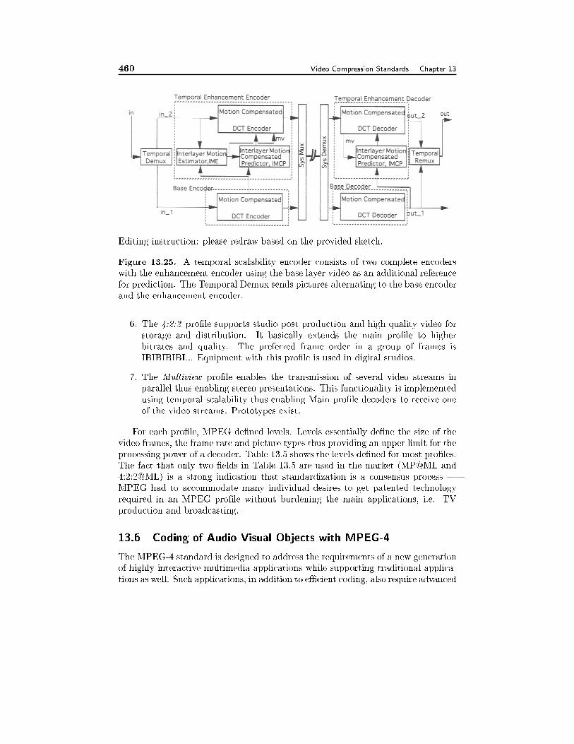
460 Video Compression Standards Chapter 13
Editing instruction: please redraw based on the provided sketch.
Figure 13.25. A temporal scalability encoder consists of two complete encoders
with the enhancement encoder using the base layer video as an additional reference
for prediction. The Temporal Demux sends pictures alternating to the base encoder
and the enhancement encoder.
6. The 4:2:2 pro�le supports studio post production and high quality video for
storage and distribution. It basically extends the main pro�le to higher
bitrates and quality. The preferred frame order in a group of frames is
IBIBIBIBI... Equipment with this pro�le is used in digital studios.
7. The Multiview pro�le enables the transmission of several video streams in
parallel thus enabling stereo presentations. This functionality is implemented
using temporal scalability thus enabling Main pro�le decoders to receive one
of the video streams. Prototypes exist.
For each pro�le, MPEG de�ned levels. Levels essentially de�ne the size of the
video frames, the frame rate and picture types thus providing an upper limit for the
processing power of a decoder. Table 13.5 shows the levels de�ned for most pro�les.
The fact that only two �elds in Table 13.5 are used in the market (MP@ML and
4:2:2@ML) is a strong indication that standardization is a consensus process |
MPEG had to accommodate many individual desires to get patented technology
required in an MPEG pro�le without burdening the main applications, i.e. TV
production and broadcasting.
13.6 Coding of Audio Visual Objects with MPEG-4
The MPEG-4 standard is designed to address the requirements of a new generation
of highly interactive multimedia applications while supporting traditional applica-
tions as well. Such applications, in addition to eÆcient coding, also require advanced
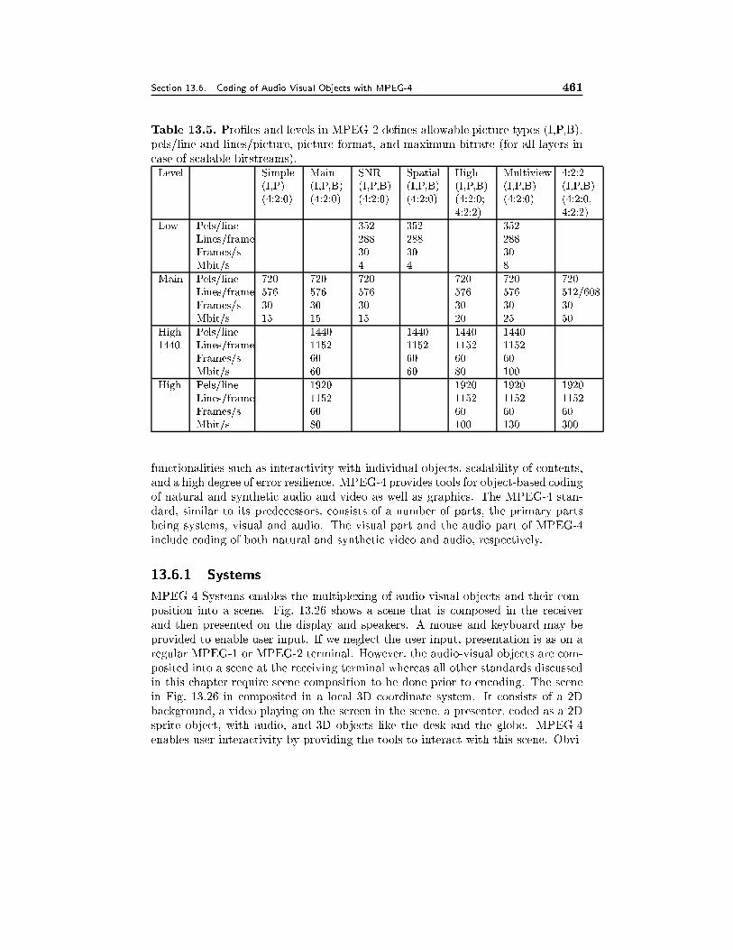
Section 13.6. Coding of Audio Visual Objects with MPEG-4 461
Table 13.5. Pro�les and levels in MPEG-2 de�nes allowable picture types (I,P,B),
pels/line and lines/picture, picture format, and maximum bitrate (for all layers in
case of scalable bitstreams).Level Simple
(I,P)
(4:2:0)
Main
(I,P,B)
(4:2:0)
SNR
(I,P,B)
(4:2:0)
Spatial
(I,P,B)
(4:2:0)
High
(I,P,B)
(4:2:0;
4:2:2)
Multiview
(I,P,B)
(4:2:0)
4:2:2
(I,P,B)
(4:2:0,
4:2:2)
Low Pels/line
Lines/frame
Frames/s
Mbit/s
352
288
30
4
352
288
30
4
352
288
30
8
Main Pels/line
Lines/frame
Frames/s
Mbit/s
720
576
30
15
720
576
30
15
720
576
30
15
720
576
30
20
720
576
30
25
720
512/608
30
50
High-
1440
Pels/line
Lines/frame
Frames/s
Mbit/s
1440
1152
60
60
1440
1152
60
60
1440
1152
60
80
1440
1152
60
100
High Pels/line
Lines/frame
Frames/s
Mbit/s
1920
1152
60
80
1920
1152
60
100
1920
1152
60
130
1920
1152
60
300
functionalities such as interactivity with individual objects, scalability of contents,
and a high degree of error resilience. MPEG-4 provides tools for object-based coding
of natural and synthetic audio and video as well as graphics. The MPEG-4 stan-
dard, similar to its predecessors, consists of a number of parts, the primary parts
being systems, visual and audio. The visual part and the audio part of MPEG-4
include coding of both natural and synthetic video and audio, respectively.
13.6.1 Systems
MPEG-4 Systems enables the multiplexing of audio-visual objects and their com-
position into a scene. Fig. 13.26 shows a scene that is composed in the receiver
and then presented on the display and speakers. A mouse and keyboard may be
provided to enable user input. If we neglect the user input, presentation is as on a
regular MPEG-1 or MPEG-2 terminal. However, the audio-visual objects are com-
posited into a scene at the receiving terminal whereas all other standards discussed
in this chapter require scene composition to be done prior to encoding. The scene
in Fig. 13.26 in composited in a local 3D coordinate system. It consists of a 2D
background, a video playing on the screen in the scene, a presenter, coded as a 2D
sprite object, with audio, and 3D objects like the desk and the globe. MPEG-4
enables user interactivity by providing the tools to interact with this scene. Obvi-
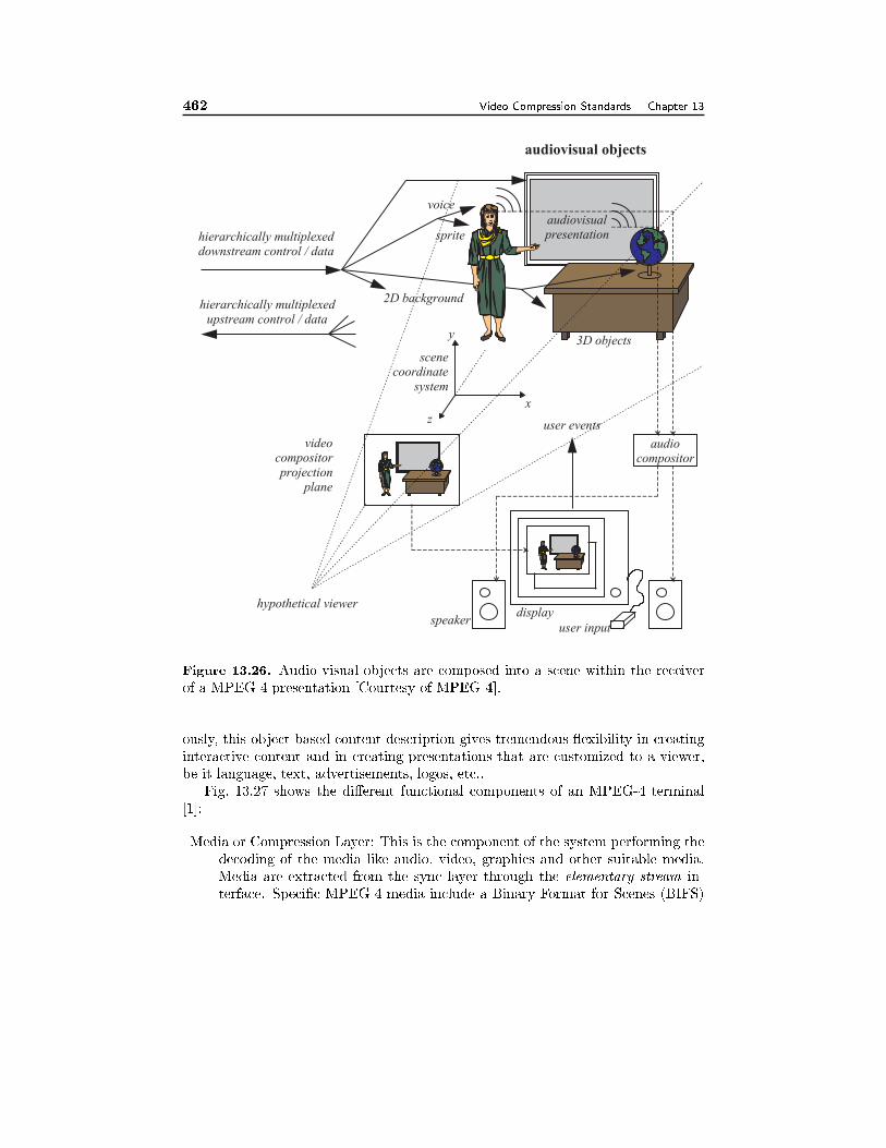
462 Video Compression Standards Chapter 13
hierarchically multiplexeddownstream control / data
hierarchically multiplexedupstream control / data
audiovisualpresentation
3D objects
2D background
voice
sprite
hypothetical viewer
projection
videocompositor
plane
audiocompositor
scenecoordinate
system
x
y
zuser events
audiovisual objects
speakerdisplay
user input
Figure 13.26. Audio-visual objects are composed into a scene within the receiver
of a MPEG-4 presentation [Courtesy of MPEG-4].
ously, this object-based content description gives tremendous exibility in creating
interactive content and in creating presentations that are customized to a viewer,
be it language, text, advertisements, logos, etc..
Fig. 13.27 shows the di�erent functional components of an MPEG-4 terminal
[1]:
Media or Compression Layer: This is the component of the system performing the
decoding of the media like audio, video, graphics and other suitable media.
Media are extracted from the sync layer through the elementary stream in-
terface. Speci�c MPEG-4 media include a Binary Format for Scenes (BIFS)
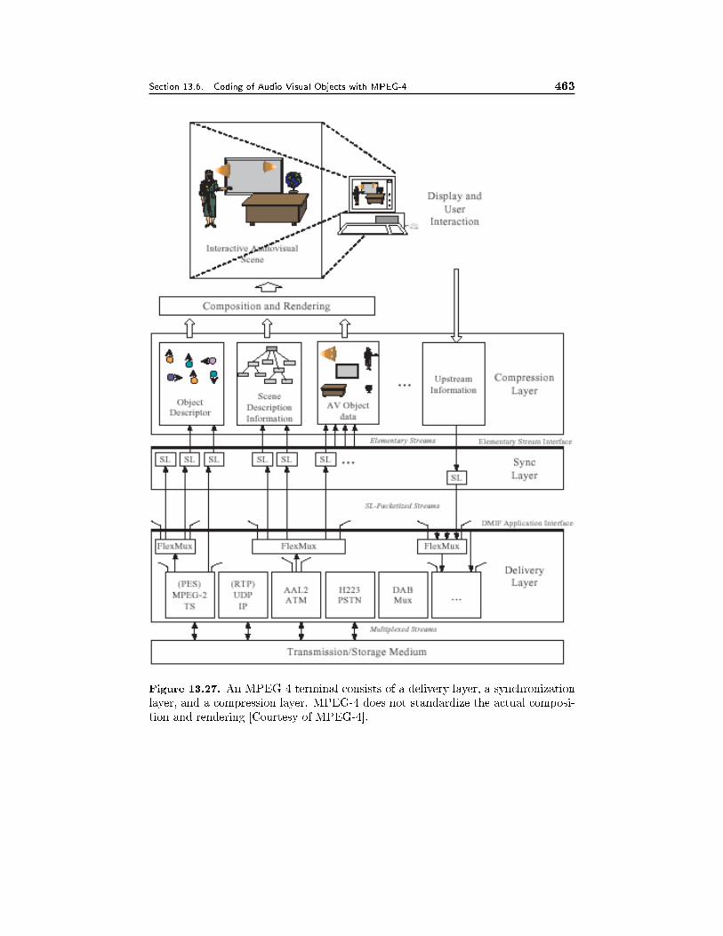
Section 13.6. Coding of Audio Visual Objects with MPEG-4 463
Figure 13.27. An MPEG-4 terminal consists of a delivery layer, a synchronization
layer, and a compression layer. MPEG-4 does not standardize the actual composi-
tion and rendering [Courtesy of MPEG-4].
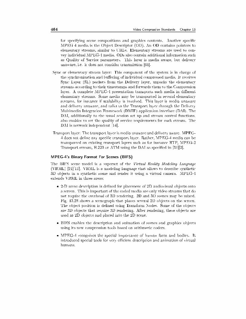
464 Video Compression Standards Chapter 13
for specifying scene compositions and graphics contents. Another speci�c
MPEG-4 media is the Object Descriptor (OD). An OD contains pointers to
elementary streams, similar to URLs. Elementary streams are used to con-
vey individual MPEG-4 media. ODs also contain additional information such
as Quality of Service parameters. This layer is media aware, but delivery
unaware, i.e. it does not consider transmission [66].
Sync or elementary stream layer: This component of the system is in charge of
the synchronization and bu�ering of individual compressed media. It receives
Sync Layer (SL) packets from the Delivery layer, unpacks the elementary
streams according to their timestamps and forwards them to the Compression
layer. A complete MPEG-4 presentation transports each media in di�erent
elementary streams. Some media may be transported in several elementary
streams, for instance if scalability is involved. This layer is media unaware
and delivery unaware, and talks to the Transport layer through the Delivery
Multimedia Integration Framework (DMIF) application interface (DAI). The
DAI, additionally to the usual session set up and stream control functions,
also enables to set the quality of service requirements for each stream. The
DAI is network independent [14].
Transport layer: The transport layer is media unaware and delivery aware. MPEG-
4 does not de�ne any speci�c transport layer. Rather, MPEG-4 media can be
transported on existing transport layers such as for instance RTP, MPEG-2
Transport stream, H.223 or ATM using the DAI as speci�ed in [31][2].
MPEG-4's Binary Format For Scenes (BIFS)
The BIFS scene model is a superset of the Virtual Reality Modeling Language
(VRML) [21][11]. VRML is a modeling language that allows to describe synthetic
3D objects in a synthetic scene and render it using a virtual camera. MPEG-4
extends VRML in three areas:
� 2-D scene description is de�ned for placement of 2D audiovisual objects onto
a screen. This is important of the coded media are only video streams that do
not require the overhead of 3D rendering. 2D and 3D scenes may be mixed.
Fig. 13.28 shows a scenegraph that places several 2D objects on the screen.
The object position is de�ned using Transform Nodes. Some of the objects
are 3D objects that require 3D rendering. After rendering, these objects are
used as 2D objects and placed into the 2D scene.
� BIFS enables the description and animation of scenes and graphics objects
using its new compression tools based on arithmetic coders.
� MPEG-4 recognizes the special importance of human faces and bodies. It
introduced special tools for very eÆcient description and animation of virtual
humans.
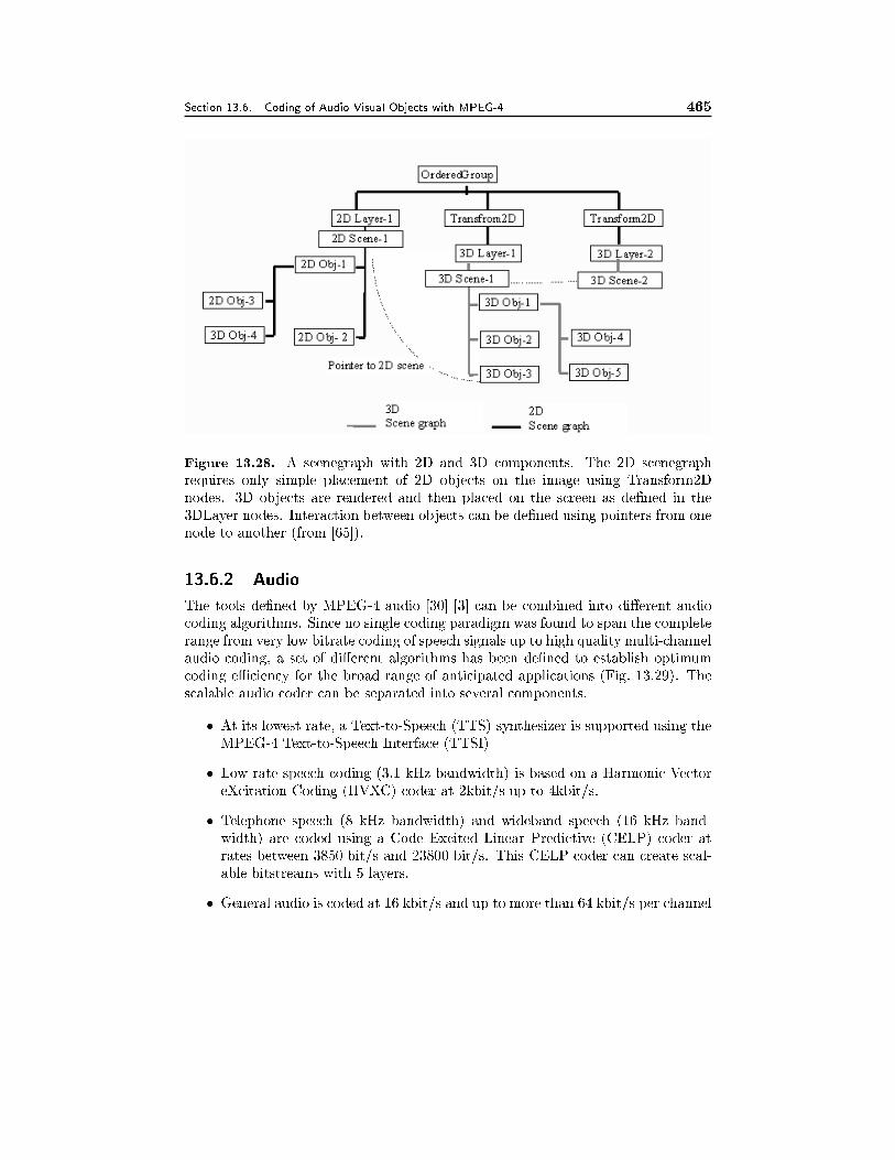
Section 13.6. Coding of Audio Visual Objects with MPEG-4 465
Figure 13.28. A scenegraph with 2D and 3D components. The 2D scenegraph
requires only simple placement of 2D objects on the image using Transform2D
nodes. 3D objects are rendered and then placed on the screen as de�ned in the
3DLayer nodes. Interaction between objects can be de�ned using pointers from one
node to another (from [65]).
13.6.2 Audio
The tools de�ned by MPEG-4 audio [30] [3] can be combined into di�erent audio
coding algorithms. Since no single coding paradigm was found to span the complete
range from very low bitrate coding of speech signals up to high quality multi-channel
audio coding, a set of di�erent algorithms has been de�ned to establish optimum
coding eÆciency for the broad range of anticipated applications (Fig. 13.29). The
scalable audio coder can be separated into several components.
� At its lowest rate, a Text-to-Speech (TTS) synthesizer is supported using the
MPEG-4 Text-to-Speech Interface (TTSI)
� Low rate speech coding (3.1 kHz bandwidth) is based on a Harmonic Vector
eXcitation Coding (HVXC) coder at 2kbit/s up to 4kbit/s.
� Telephone speech (8 kHz bandwidth) and wideband speech (16 kHz band-
width) are coded using a Code Excited Linear Predictive (CELP) coder at
rates between 3850 bit/s and 23800 bit/s. This CELP coder can create scal-
able bitstreams with 5 layers.
� General audio is coded at 16 kbit/s and up to more than 64 kbit/s per channel
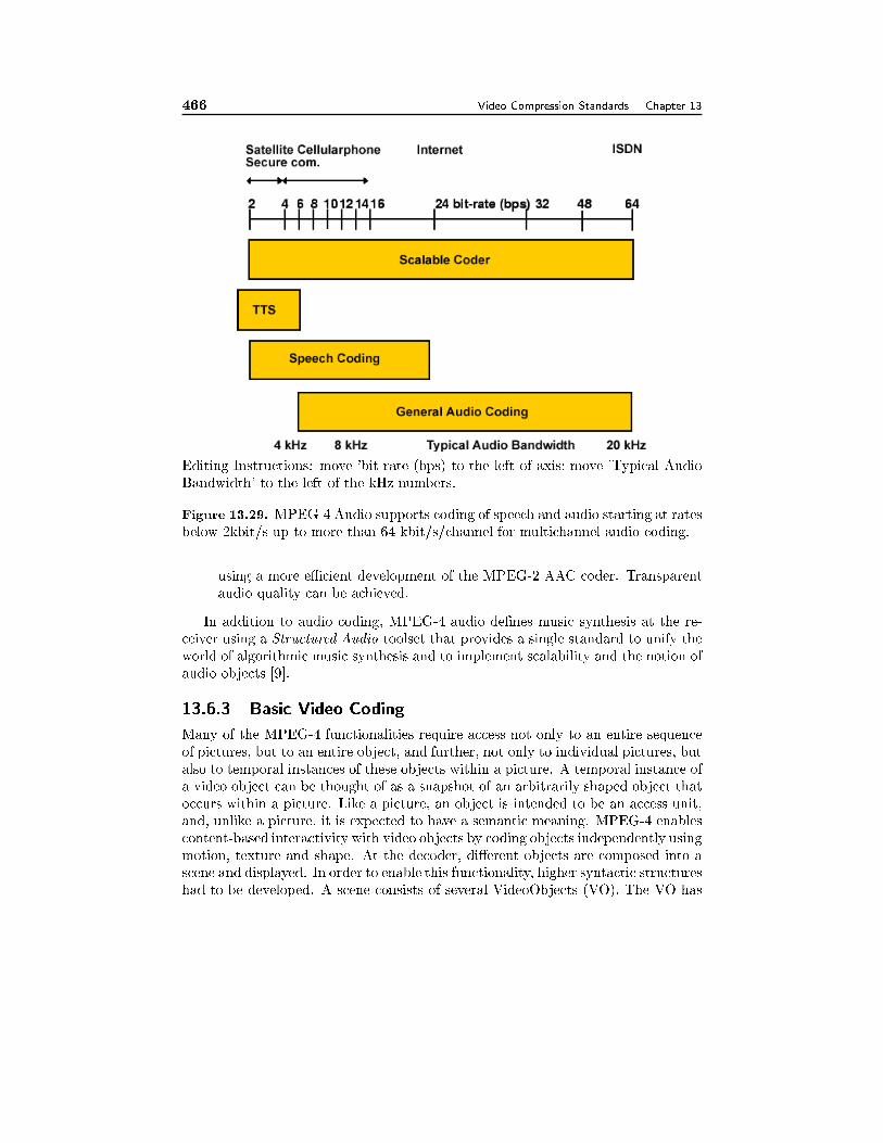
466 Video Compression Standards Chapter 13
Editing Instructions: move 'bit-rate (bps) to the left of axis; move 'Typical Audio
Bandwidth' to the left of the kHz numbers.
Figure 13.29. MPEG-4 Audio supports coding of speech and audio starting at rates
below 2kbit/s up to more than 64 kbit/s/channel for multichannel audio coding.
using a more eÆcient development of the MPEG-2 AAC coder. Transparent
audio quality can be achieved.
In addition to audio coding, MPEG-4 audio de�nes music synthesis at the re-
ceiver using a Structured Audio toolset that provides a single standard to unify the
world of algorithmic music synthesis and to implement scalability and the notion of
audio objects [9].
13.6.3 Basic Video Coding
Many of the MPEG-4 functionalities require access not only to an entire sequence
of pictures, but to an entire object, and further, not only to individual pictures, but
also to temporal instances of these objects within a picture. A temporal instance of
a video object can be thought of as a snapshot of an arbitrarily shaped object that
occurs within a picture. Like a picture, an object is intended to be an access unit,
and, unlike a picture, it is expected to have a semantic meaning. MPEG-4 enables
content-based interactivity with video objects by coding objects independently using
motion, texture and shape. At the decoder, di�erent objects are composed into a
scene and displayed. In order to enable this functionality, higher syntactic structures
had to be developed. A scene consists of several VideoObjects (VO). The VO has
Section 13.6. Coding of Audio Visual Objects with MPEG-4 467
3 dimensions (2D+time). A VO can be composed of several VideoObjectLayers
(VOL). Each VOL (2D+time) represents various instantiations of a VO. A VOL
can represent di�erent layers of a scalable bitstream or di�erent parts of a VO. A
time instant of a VOL is called VideoObjectPlane (VOP). A VOP is a rectangular
video frame or a part thereof. It can be fully described by its texture variations
(a set of luminance and chrominance values) and its shape. The video encoder
applies the motion, texture and shape coding tools to the VOP using I, P, and B
modes similar to the modes of MPEG-2. For editing and random access purposes,
consecutive VOPs can be grouped into a GroupOfVideoObjectPlanes (GVOP). A
video session, the highest syntactic structure, may consist of several VOs.
The example in Fig. 13.30 shows one VO composed of 2 VOL. VOL1 consists
of the tree and the background. VOL2 represents the person. In the example,
VOL1 is represented by two separate VOPs, VOP1 and VOP3. Hence, VOL1
may provide content-based scalability in the sense that a decoder may choose not
to decode one VOP of VOL1 due to resource limitations. VOL2 contains just one
VOP, namely VOP2. VOP2 may be represented using a temporal, spatial or quality
scalable bitstream. In this case, a decoder might again decide to decode only the
lower layers of VOL 2. The example in Fig. 13.30 shows the complex structures
of content-based access and scalability that MPEG-4 supports. However, the given
example could also be represented in a straight forward fashion with three VOs.
The background, the tree and the person are coded as separate VOs with one layer
each, and each layer is represented by one VOP. The VOPs are encoded separately
and composed in a scene at the decoder.
To see how MPEG-4 video coding works, consider a sequence of VOPs. Extend-
ing the concept of intra (I-) pictures, predictive (P-) and bidirectionally predictive
(B-) pictures of MPEG-1/2 to VOPs, I-VOP, P-VOP and B-VOP result. If, two
consecutive B-VOPs are used between a pair of reference VOPs (I- or a P-VOPs),
the resulting coding structure is as shown in Fig. 13.31.
Coding EÆciency Tools
In addition to the obvious changes due to the object-based nature of MPEG-4, the
following tools were introduced in order to increase coding eÆciency compared to
MPEG-1 and MPEG-2:
DC Prediction: This is improved compared to MPEG1/2. Either the previous
block or the block above the current block can be chosen as predictors to
predict the current DC value.
AC Prediction: AC prediction of DCT coeÆcients is new in MPEG-4. The block
that was chosen to predict the DC-coeÆcient is also used for predicting one line
of AC coeÆcients. If the predictor is the previous block, the AC coeÆcients
of its �rst column are used to predict the co-located AC coeÆcients of the
current block. If the predictor is the block from the previous row, it is used to
predict the �rst row of AC coeÆcients. AC prediction does not work well for

468 Video Compression Standards Chapter 13
VOP1
VOL2VOP3VOP2
VOL1
Figure 13.30. Object-based coding requires the decoder to compose di�erent
VideoObjectPlanes (VOP) into a scene. VideoObjectLayers (VOL) enable content-
based scalability.
B PBI
BackwardPrediction
ForwardPrediction
Figure 13.31. An example prediction structure using I, P and B-VOPs (from [59]).
blocks with coarse texture or diagonal edges or horizontal as well as vertical
edges. Switching AC prediction on and o� on a block level is desirable but
too costly. Consequently, the decision is made on the MB level.
Alternate Horizontal Scan: This scan is added to the two scans of MPEG-2
(Fig. 13.19). The Alternate Scan of MPEG-2 is referred to as Alternate Verti-
cal Scan in MPEG-4. The Alternate Horizontal Scan is created by mirroring
the Vertical Scan. The scan is selected at the same time as the AC prediction
is decided. In case of AC prediction from the previous block, Alternate Verti-
cal Scan is selected. In case of AC prediction from the block above, Alternate
Horizontal Scan is used. No AC prediction is coupled to the Zigzag scan.
3D VLC: Coding of DCT coeÆcients is achieved similar to H.263.
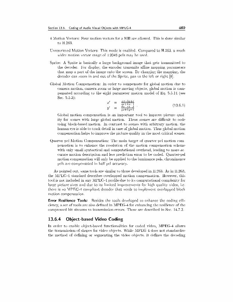
Section 13.6. Coding of Audio Visual Objects with MPEG-4 469
4 Motion Vectors: Four motion vectors for a MB are allowed. This is done similar
to H.263.
Unrestricted Motion Vectors: This mode is enabled. Compared to H.263, a much
wider motion vector range of �2048 pels may be used.
Sprite: A Sprite is basically a large background image that gets transmitted to
the decoder. For display, the encoder transmits aÆne mapping parameters
that map a part of the image onto the screen. By changing the mapping, the
decoder can zoom in and out of the Sprite, pan to the left or right [8].
Global Motion Compensation: In order to compensate for global motion due to
camera motion, camera zoom or large moving objects, global motion is com-
pensated according to the eight parameter motion model of Eq. 5.5.14 (see
Sec. 5.5.3):
x0 = ax+by+c
gx+hy+1
y0 = dx+ey+f
gx+hy+1
: (13.6.1)
Global motion compensation is an important tool to improve picture qual-
ity for scenes with large global motion. These scenes are diÆcult to code
using block-based motion. In contrast to scenes with arbitrary motion, the
human eye is able to track detail in case of global motion. Thus global motion
compensation helps to improve the picture quality in the most critical scenes.
Quarter-pel Motion Compensation: The main target of quarter-pel motion com-
pensation is to enhance the resolution of the motion compensation scheme
with only small syntactical and computational overhead, leading to more ac-
curate motion description and less prediction error to be coded. Quarter-pel
motion compensation will only be applied to the luminance pels, chrominance
pels are compensated in half pel accuracy.
As pointed out, some tools are similar to those developed in H.263. As in H.263,
the MPEG-4 standard describes overlapped motion compensation. However, this
tool is not included in any MPEG-4 pro�le due to its computational complexity for
large picture sizes and due to its limited improvements for high quality video, i.e.
there is no MPEG-4 compliant decoder that needs to implement overlapped block
motion compensation.
Error Resilience Tools: Besides the tools developed to enhance the coding eÆ-
ciency, a set of tools are also de�ned in MPEG-4 for enhancing the resilience of the
compressed bit streams to transmission errors. These are described in Sec. 14.7.2.
13.6.4 Object-based Video Coding
In order to enable object-based functionalities for coded video, MPEG-4 allows
the transmission of shapes for video objects. While MPEG-4 does not standardize
the method of de�ning or segmenting the video objects, it de�nes the decoding
470 Video Compression Standards Chapter 13
algorithm and implicitly an encoding algorithm for describing the shape. Shape is
described using alpha-maps that have the same resolution as the luminance signal.
An alpha map is co-located with the luminance picture. MPEG-4 de�nes the alpha-
map as two parts. The binary alpha-map de�nes pels that belong to the object.
In case of grey-scale alpha maps, we have an additional alpha map that de�nes
the transparency using 8 bits/pel. Alpha-maps extend a macroblock. The 16 � 16binary alpha-map of a MB is called Binary Alpha Block (BAB). In the following,
we describe the individual tools that MPEG-4 uses for object-based video coding.
Binary Shape: A context-based arithmetic coder as described in Sec. 10.1.1 is used
to code boundary blocks of an object. A boundary block contains pels of the
object and of the background. It is co-located with a MB. For non-boundary
blocks, the encoder just signals whether the MB is part of the object or not.
A sequence of alpha-maps may be coded and transmitted without texture.
Alternatively, MPEG-4 uses tools like padding and DCT or SA-DCT to code
the texture that goes with the object. BABs are coded in intra-mode and
inter-mode. Motion compensation may be used in inter mode. Shape motion
vector coding uses the motion vectors associated with the texture coding as a
predictor.
Padding: In order to code the texture of BABs using block-based DCT, the texture
of the background may be set to any color. In intra mode, this background
color has no e�ect on the decoded pictures and can be choosen by the encoder.
However, for motion compensation, the motion vector of the current block
may refer to a boundary block in the previous reference picture. Part of the
background pels of the reference picture might be located in the area of the
current object - hence the value of these background pictures in uences the
prediction loop. MPEG-4 uses padding as described in Sec. 10.2.1 to de�ne
the background pels used in prediction.
Shape Adaptive DCT: The encoder may choose to use SA-DCT for coding the
texture of BABs (Sec. 10.2.2). However, padding of the motion compensated
prediction image is still required.
Greyscale Shape Coding: MPEG-4 allows the transmission of arbitrary alpha-
maps. Since the alpha-maps are de�ned with 8 bits, they are coded the same
way as the luminance signal.
Fig. 13.32a shows the block diagram of the object-based MPEG-4 video coder.
MPEG-4 uses two types of motion vectors: In Fig. 13.32, we name the conven-
tional motion vectors used to compensate the motion of texture Texture Motion.
Motion vectors describing the shift of the object shape are called Shape Motion. A
shape motion vector may be associated to a BAB. Image analysis estimates texture
and shape motion of the current VOP Sk with respect to the reference VOP S0
k�1.
Parameter coding encodes the parameters predictively. The parameters get trans-
mitted, decoded and the new reference VOP is stored in the VOP memory. The
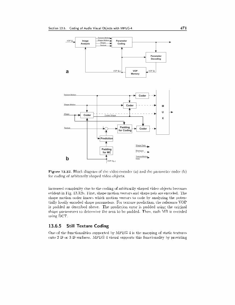
Section 13.6. Coding of Audio Visual Objects with MPEG-4 471
Image
Analysis
VOP
Memory
Parameter
Coding
Parameter
Decoding
Texture Motion
Shape Motion
Shape
Texture
VOP Sk
VOP S’k-1 VOP S’ka
Texture Motion
Shape Motion
Shape
Texture
VOP S’k-1
Prediction
Paddingfor Coding
Coder M
U
X
Coder
Coder
Padding
for MC
Coder
Shape Data
Bitstream
Texture/Motion
Data
Coded Shape
+
-
b
Figure 13.32. Block diagram of the video encoder (a) and the parameter coder (b)
for coding of arbitrarily shaped video objects.
increased complexity due to the coding of arbitrarily shaped video objects becomes
evident in Fig. 13.32b. First, shape motion vectors and shape pels are encoded. The
shape motion coder knows which motion vectors to code by analyzing the poten-
tially lossily encoded shape parameters. For texture prediction, the reference VOP
is padded as described above. The prediction error is padded using the original
shape parameters to determine the area to be padded. Then, each MB is encoded
using DCT.
13.6.5 Still Texture Coding
One of the functionalities supported by MPEG-4 is the mapping of static textures
onto 2-D or 3-D surfaces. MPEG-4 visual supports this functionality by providing
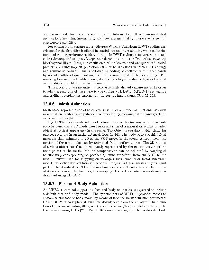
472 Video Compression Standards Chapter 13
a separate mode for encoding static texture information. It is envisioned that
applications involving interactivity with texture mapped synthetic scenes require
continuous scalability.
For coding static texture maps, Discrete Wavelet Transform (DWT) coding was
selected for the exibility it o�ered in spatial and quality scalability while maintain-
ing good coding performance (Sec. 11.3.1). In DWT coding, a texture map image
is �rst decomposed using a 2D separable decomposition using Daubechies (9,3)-tap
biorthogonal �lters. Next, the coeÆcients of the lowest band are quantized, coded
predictively using implicit prediction (similar to that used in intra DCT coding)
and arithmetic coding. This is followed by coding of coeÆcients of higher bands
by use of multilevel quantization, zero-tree scanning and arithmetic coding. The
resulting bitstream is exibly arranged allowing a large number of layers of spatial
and quality scalability to be easily derived.
This algorithm was extended to code arbitrarily shaped texture maps. In order
to adapt a scan line of the shape to the coding with DWT, MPEG-4 uses leading
and trailing boundary extensions that mirror the image signal (Sec. 11.3.1).
13.6.6 Mesh Animation
Mesh based representation of an object is useful for a number of functionalities such
as animation, content manipulation, content overlay, merging natural and synthetic
video and others [67].
Fig. 13.33 shows a mesh coder and its integration with a texture coder. The mesh
encoder generates a 2D mesh based representation of a natural or synthetic video
object at its �rst appearance in the scene. The object is tesselated with triangular
patches resulting in an initial 2D mesh (Fig. 13.34). The node points of this initial
mesh are then animated in 2D as the VOP moves in the scene. Alternatively, the
motion of the node point can by animated from another source. The 2D motion
of a video object can thus be compactly represented by the motion vectors of the
node points of the mesh. Motion compensation can be achieved by warping of
texture map corresponding to patches by aÆne transform from one VOP to the
next. Texture used for mapping on to object mesh models or facial wireframe
models are either derived from video or still images. Whereas mesh analysis is not
part of the standard, MPEG-4 de�nes how to encode 2D meshes and the motion
of its node points. Furthermore, the mapping of a texture onto the mesh may be
described using MPEG-4.
13.6.7 Face and Body Animation
An MPEG-4 terminal supporting face and body animation is expected to include
a default face and body model. The systems part of MPEG-4 provides means to
customize this face or body model by means of face and body de�nition parameters
(FDP, BDP) or to replace it with one downloaded from the encoder. The de�ni-
tion of a scene including 3D geometry and of a face/body model can be sent to
the receiver using BIFS [23]. Fig. 13.35 shows a scenegraph that a decoder built
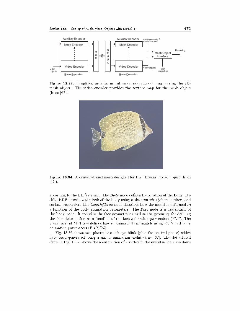
Section 13.6. Coding of Audio Visual Objects with MPEG-4 473
Video Encodervideoobjects
video objects
Mesh Object
Interface
userinteraction
Rendering
Mesh Encoder
Video Decoder
Mesh Decoder
Auxiliary Encoder
Base Encoder
Auxiliary Decoder
Base Decoder
mesh geometry &motion vectors
M
U
X
D
E
M
U
X
Figure 13.33. Simpli�ed architecture of an encoder/decoder supporting the 2D-
mesh object. The video encoder provides the texture map for the mesh object
(from [67]).
Figure 13.34. A content-based mesh designed for the "Bream" video object (from
[67]).
according to the BIFS stream. The Body node de�nes the location of the Body. It's
child BDP describes the look of the body using a skeleton with joints, surfaces and
surface properties. The bodyDefTable node describes how the model is deformed as
a function of the body animation parameters. The Face node is a descendent of
the body node. It contains the face geometry as well as the geometry for de�ning
the face deformation as a function of the face animation parameters (FAP). The
visual part of MPEG-4 de�nes how to animate these models using FAPs and body
animation parameters (BAP)[24].
Fig. 13.36 shows two phases of a left eye blink (plus the neutral phase) which
have been generated using a simple animation architecture [67]. The dotted half
circle in Fig. 13.36 shows the ideal motion of a vertex in the eyelid as it moves down
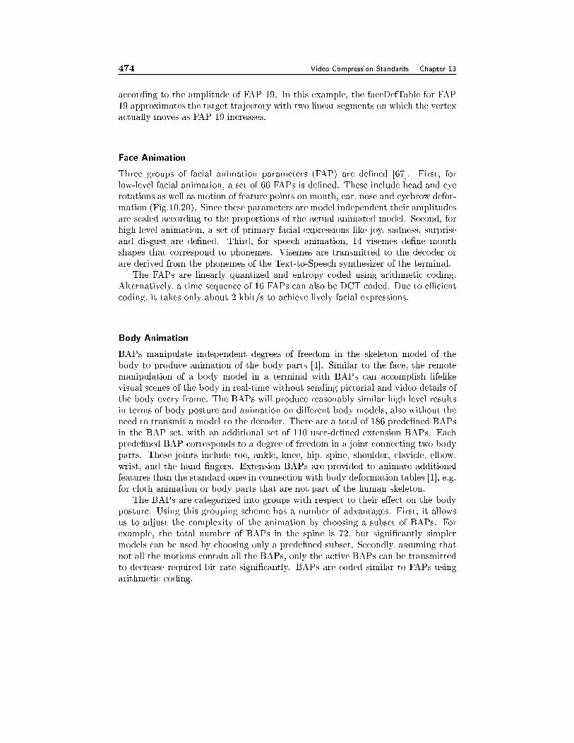
474 Video Compression Standards Chapter 13
according to the amplitude of FAP 19. In this example, the faceDefTable for FAP
19 approximates the target trajectory with two linear segments on which the vertex
actually moves as FAP 19 increases.
Face Animation
Three groups of facial animation parameters (FAP) are de�ned [67]. First, for
low-level facial animation, a set of 66 FAPs is de�ned. These include head and eye
rotations as well as motion of feature points on mouth, ear, nose and eyebrow defor-
mation (Fig.10.20). Since these parameters are model independent their amplitudes
are scaled according to the proportions of the actual animated model. Second, for
high-level animation, a set of primary facial expressions like joy, sadness, surprise
and disgust are de�ned. Third, for speech animation, 14 visemes de�ne mouth
shapes that correspond to phonemes. Visemes are transmitted to the decoder or
are derived from the phonemes of the Text-to-Speech synthesizer of the terminal.
The FAPs are linearly quantized and entropy coded using arithmetic coding.
Alternatively, a time sequence of 16 FAPs can also be DCT coded. Due to eÆcient
coding, it takes only about 2 kbit/s to achieve lively facial expressions.
Body Animation
BAPs manipulate independent degrees of freedom in the skeleton model of the
body to produce animation of the body parts [4]. Similar to the face, the remote
manipulation of a body model in a terminal with BAPs can accomplish lifelike
visual scenes of the body in real-time without sending pictorial and video details of
the body every frame. The BAPs will produce reasonably similar high level results
in terms of body posture and animation on di�erent body models, also without the
need to transmit a model to the decoder. There are a total of 186 prede�ned BAPs
in the BAP set, with an additional set of 110 user-de�ned extension BAPs. Each
prede�ned BAP corresponds to a degree of freedom in a joint connecting two body
parts. These joints include toe, ankle, knee, hip, spine, shoulder, clavicle, elbow,
wrist, and the hand �ngers. Extension BAPs are provided to animate additional
features than the standard ones in connection with body deformation tables [1], e.g.
for cloth animation or body parts that are not part of the human skeleton.
The BAPs are categorized into groups with respect to their e�ect on the body
posture. Using this grouping scheme has a number of advantages. First, it allows
us to adjust the complexity of the animation by choosing a subset of BAPs. For
example, the total number of BAPs in the spine is 72, but signi�cantly simpler
models can be used by choosing only a prede�ned subset. Secondly, assuming that
not all the motions contain all the BAPs, only the active BAPs can be transmitted
to decrease required bit rate signi�cantly. BAPs are coded similar to FAPs using
arithmetic coding.
Section 13.6. Coding of Audio Visual Objects with MPEG-4 475
Body
BDP BAPrenderedBody
FBA
Stream
bodySceneGraph
bodyDefTable
Joint Joint
Joint Face
FDP FAPrenderedFace
faceSceneGraph
faceDefTable
faceDefMesh
faceDefTransform
IFS
IFS
BIFS
Stream
BIFS
Decoder
FBA
Decoder
Figure 13.35. The scenegraph describing a human body is transmitted in a BIFS
stream. The nodes Body and Face are animated using the FAP's and BAP's of
the FBA stream. The BDP and FDP nodes and their children describe the virtual
human (from [4]).
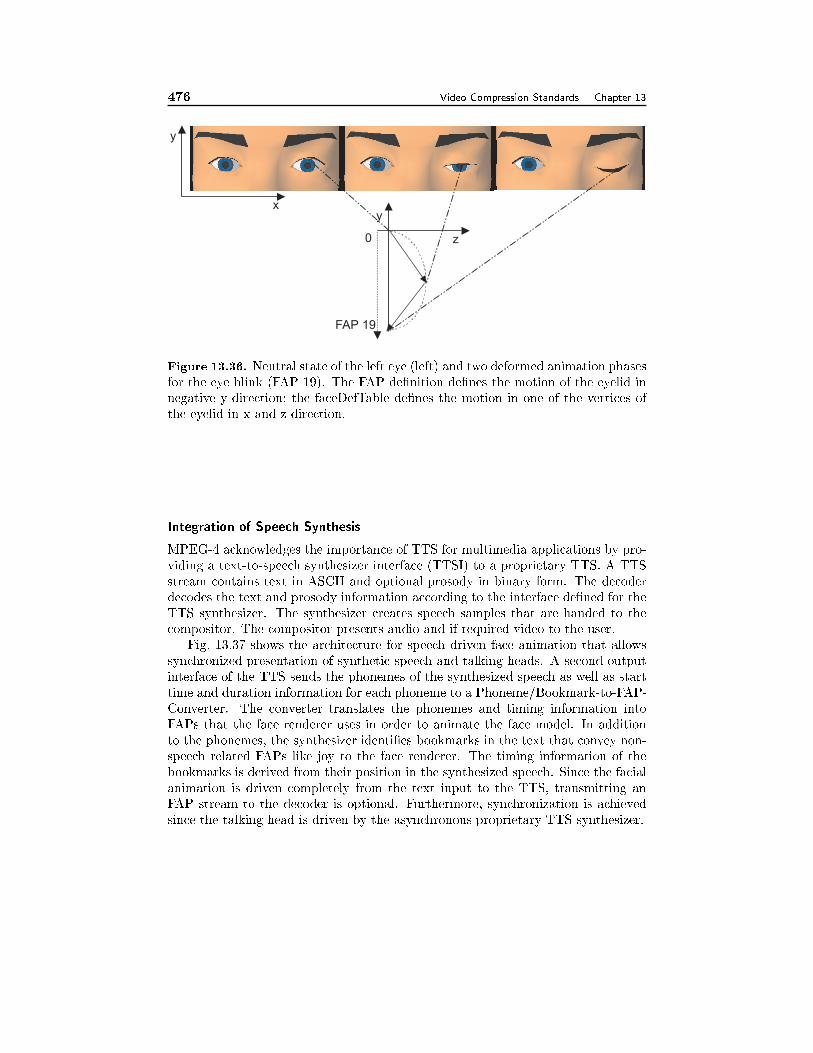
476 Video Compression Standards Chapter 13
x
y
y
z
FAP 19
0
Figure 13.36. Neutral state of the left eye (left) and two deformed animation phases
for the eye blink (FAP 19). The FAP de�nition de�nes the motion of the eyelid in
negative y-direction; the faceDefTable de�nes the motion in one of the vertices of
the eyelid in x and z direction.
Integration of Speech Synthesis
MPEG-4 acknowledges the importance of TTS for multimedia applications by pro-
viding a text-to-speech synthesizer interface (TTSI) to a proprietary TTS. A TTS
stream contains text in ASCII and optional prosody in binary form. The decoder
decodes the text and prosody information according to the interface de�ned for the
TTS synthesizer. The synthesizer creates speech samples that are handed to the
compositor. The compositor presents audio and if required video to the user.
Fig. 13.37 shows the architecture for speech driven face animation that allows
synchronized presentation of synthetic speech and talking heads. A second output
interface of the TTS sends the phonemes of the synthesized speech as well as start
time and duration information for each phoneme to a Phoneme/Bookmark-to-FAP-
Converter. The converter translates the phonemes and timing information into
FAPs that the face renderer uses in order to animate the face model. In addition
to the phonemes, the synthesizer identi�es bookmarks in the text that convey non-
speech related FAPs like joy to the face renderer. The timing information of the
bookmarks is derived from their position in the synthesized speech. Since the facial
animation is driven completely from the text input to the TTS, transmitting an
FAP stream to the decoder is optional. Furthermore, synchronization is achieved
since the talking head is driven by the asynchronous proprietary TTS synthesizer.

Section 13.6. Coding of Audio Visual Objects with MPEG-4 477
DecoderSpeeech
Phoneme/Bookmarkto FAP Converter
FaceRenderer
ProprietarySpeech
Synthesizer
Com
posito
r
Audio
Video
TTS Stream
Face Model
Phonemes
Bookmarks
Editing Instructions: Replace 'Proprietary Speech Synthesizer' with 'Text to Speech
Synthesizer'; Add 'FAPs' to arrow at output of the block 'Phoneme/Bookmark ...'.
Figure 13.37. MPEG-4 architecture for face animation allowing synchronization of
facial expressions and speech generated by a proprietary text-to-speech synthesizer.
13.6.8 Pro�les
MPEG-4 developed an elaborate structure of pro�les. As indicated in Fig. 13.38, a
MPEG-4 terminal has to implement several pro�les. An object descriptor pro�le is
required to enable the transport of MPEG-4 streams and identify these streams in
the terminal. A scene description pro�le provides the tools, to compose the audio,
video or graphics objects into a scene. A 2D scene description pro�le enables just
the placement of 2D video objects, higher pro�les provide more functionality. A
media pro�le needs to be implemented in order to present actual content on the
terminal. MPEG-4 supports audio, video and graphics as media. Several video
pro�les are de�ned. Here, we list only a subset of them and mention their main
functionalities.
Simple Pro�le: The Simple pro�le was created with low complexity applications in
mind. The �rst usage is mobile use of (audio)visual services, and the second
is putting very low complexity video on the Internet. It supports up to four
objects in the scene with, at the lowest level, a maximum total size of a QCIF
picture. There are 3 levels for the Simple Pro�le with bitrates from 64 to
384 kbit/s. It provides the following tools: I-, P-VOPs, AC/DC prediction,
4 motion vectors, unrestricted motion vectors, slice resynchronization, data
partitioning and reversible VLC. This pro�le is able to decode H.263 video
streams that do not use any of the optional annexes of H.263.
Simple Scalable Pro�le: This pro�le adds support for B-frames, temporal scala-
bility and spatial scalability to the Simple pro�le. This pro�le is useful for
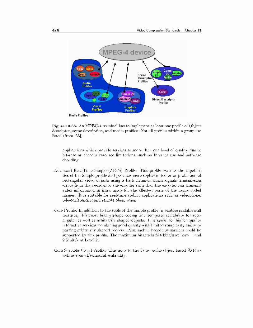
478 Video Compression Standards Chapter 13
Figure 13.38. An MPEG-4 terminal has to implement at least one pro�le of Object
descriptor, scene description, and media pro�les. Not all pro�les within a group are
listed (from [53]).
applications which provide services at more than one level of quality due to
bit-rate or decoder resource limitations, such as Internet use and software
decoding.
Advanced Real-Time Simple (ARTS) Pro�le: This pro�le extends the capabili-
ties of the Simple pro�le and provides more sophisticated error protection of
rectangular video objects using a back-channel, which signals transmission
errors from the decoder to the encoder such that the encoder can transmit
video information in intra mode for the a�ected parts of the newly coded
images. It is suitable for real-time coding applications such as videophone,
tele-conferencing and remote observation.
Core Pro�le: In addition to the tools of the Simple pro�le, it enables scalable still
textures, B-frames, binary shape coding and temporal scalability for rect-
angular as well as arbitrarily shaped objects. It is useful for higher quality
interactive services, combining good quality with limited complexity and sup-
porting arbitrarily shaped objects. Also mobile broadcast services could be
supported by this pro�le. The maximum bitrate is 384 kbit/s at Level 1 and
2 Mbit/s at Level 2.
Core Scalable Visual Pro�le: This adds to the Core pro�le object based SNR as
well as spatial/temporal scalability.
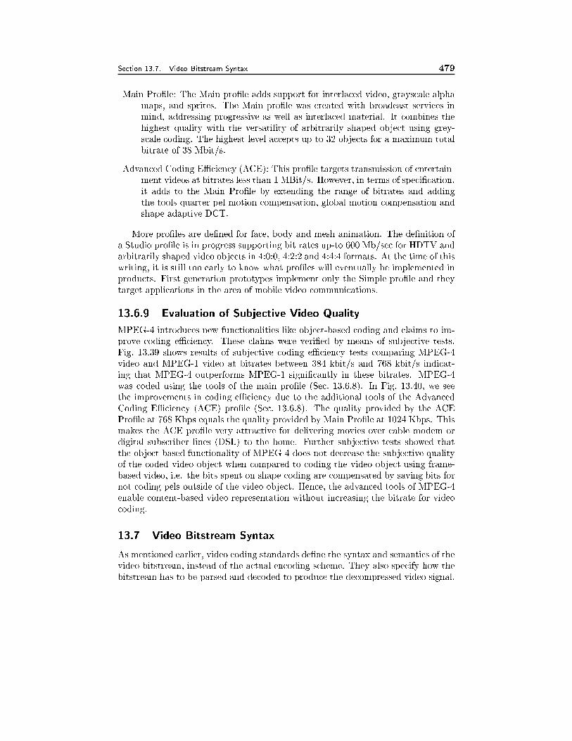
Section 13.7. Video Bitstream Syntax 479
Main Pro�le: The Main pro�le adds support for interlaced video, grayscale alpha
maps, and sprites. The Main pro�le was created with broadcast services in
mind, addressing progressive as well as interlaced material. It combines the
highest quality with the versatility of arbitrarily shaped object using grey-
scale coding. The highest level accepts up to 32 objects for a maximum total
bitrate of 38 Mbit/s.
Advanced Coding EÆciency (ACE): This pro�le targets transmission of entertain-
ment videos at bitrates less than 1 MBit/s. However, in terms of speci�cation,
it adds to the Main Pro�le by extending the range of bitrates and adding
the tools quarter pel motion compensation, global motion compensation and
shape adaptive DCT.
More pro�les are de�ned for face, body and mesh animation. The de�nition of
a Studio pro�le is in progress supporting bit rates up-to 600 Mb/sec for HDTV and
arbitrarily shaped video objects in 4:0:0, 4:2:2 and 4:4:4 formats. At the time of this
writing, it is still too early to know what pro�les will eventually be implemented in
products. First generation prototypes implement only the Simple pro�le and they
target applications in the area of mobile video communications.
13.6.9 Evaluation of Subjective Video Quality
MPEG-4 introduces new functionalities like object-based coding and claims to im-
prove coding eÆciency. These claims were veri�ed by means of subjective tests.
Fig. 13.39 shows results of subjective coding eÆciency tests comparing MPEG-4
video and MPEG-1 video at bitrates between 384 kbit/s and 768 kbit/s indicat-
ing that MPEG-4 outperforms MPEG-1 signi�cantly in these bitrates. MPEG-4
was coded using the tools of the main pro�le (Sec. 13.6.8). In Fig. 13.40, we see
the improvements in coding eÆciency due to the additional tools of the Advanced
Coding EÆciency (ACE) pro�le (Sec. 13.6.8). The quality provided by the ACE
Pro�le at 768 Kbps equals the quality provided by Main Pro�le at 1024 Kbps. This
makes the ACE pro�le very attractive for delivering movies over cable modem or
digital subscriber lines (DSL) to the home. Further subjective tests showed that
the object-based functionality of MPEG-4 does not decrease the subjective quality
of the coded video object when compared to coding the video object using frame-
based video, i.e. the bits spent on shape coding are compensated by saving bits for
not coding pels outside of the video object. Hence, the advanced tools of MPEG-4
enable content-based video representation without increasing the bitrate for video
coding.
13.7 Video Bitstream Syntax
As mentioned earlier, video coding standards de�ne the syntax and semantics of the
video bitstream, instead of the actual encoding scheme. They also specify how the
bitstream has to be parsed and decoded to produce the decompressed video signal.
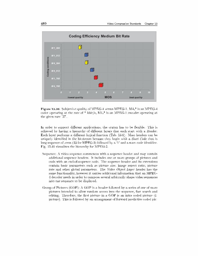
480 Video Compression Standards Chapter 13
0 1 2 3 4 5 6 7 8 9 10
lowest quality MOS best quality
M 4_768
M 1_768
M 4_512
M 4_384
M 1_512
M 1_384C
od
ing
co
nd
itio
ns
Coding Efficiency Medium Bit Rate
Figure 13.39. Subjective quality of MPEG-4 versus MPEG-1. M4 * is an MPEG-4
coder operating at the rate of * kbit/s, M1 * is an MPEG-1 encoder operating at
the given rate [27].
In order to support di�erent applications, the syntax has to be exible. This is
achieved by having a hierarchy of di�erent layers that each start with a Header.
Each layer performs a di�erent logical function (Tab. 13.6). Most headers can be
uniquely identi�ed in the bitstream because they begin with a Start Code that is
long sequence of zeros (23 for MPEG-2) followed by a '1' and a start code identi�er.
Fig. 13.41 visualizes the hierarchy for MPEG-2.
Sequence: A video sequence commences with a sequence header and may contain
additional sequence headers. It includes one or more groups of pictures and
ends with an end-of-sequence code. The sequence header and its extensions
contain basic parameters such as picture size, image aspect ratio, picture
rate and other global parameters. The Video Object Layer header has the
same functionality, however it carries additional information that an MPEG-
4 decoder needs in order to compose several arbitrarily shape video sequences
into one sequence to be displayed.
Group of Pictures (GOP): A GOP is a header followed by a series of one of more
pictures intended to allow random access into the sequence, fast search and
editing. Therefore, the �rst picture in a GOP is an intra-coded picture (I-
picture). This is followed by an arrangement of forward-predictive coded pic-
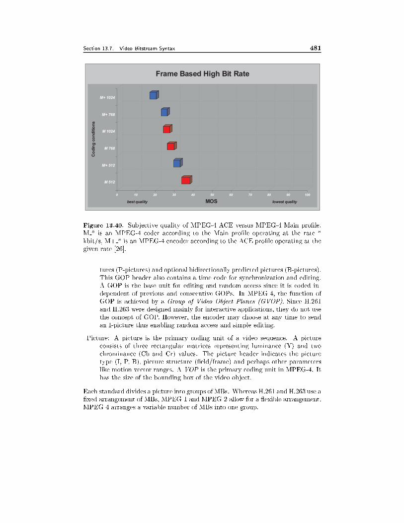
Section 13.7. Video Bitstream Syntax 481
0 10 20 30 40 50 60 70 80 90 100
best quality MOS lowest quality
M 512
M+ 512
M 768
M 1024
M+ 768
M+ 1024C
od
ing
co
nd
itio
ns
Frame Based High Bit Rate
Figure 13.40. Subjective quality of MPEG-4 ACE versus MPEG-4 Main pro�le.
M * is an MPEG-4 coder according to the Main pro�le operating at the rate *
kbit/s, M+ * is an MPEG-4 encoder according to the ACE pro�le operating at the
given rate [26].
tures (P-pictures) and optional bidirectionally predicted pictures (B-pictures).
This GOP header also contains a time code for synchronization and editing.
A GOP is the base unit for editing and random access since it is coded in-
dependent of previous and consecutive GOPs. In MPEG-4, the function of
GOP is achieved by a Group of Video Object Planes (GVOP). Since H.261
and H.263 were designed mainly for interactive applications, they do not use
the concept of GOP. However, the encoder may choose at any time to send
an I-picture thus enabling random access and simple editing.
Picture: A picture is the primary coding unit of a video sequence. A picture
consists of three rectangular matrices representing luminance (Y) and two
chrominance (Cb and Cr) values. The picture header indicates the picture
type (I, P, B), picture structure (�eld/frame) and perhaps other parameters
like motion vector ranges. A VOP is the primary coding unit in MPEG-4. It
has the size of the bounding box of the video object.
Each standard divides a picture into groups of MBs. Whereas H.261 and H.263 use a
�xed arrangement of MBs, MPEG-1 and MPEG-2 allow for a exible arrangement.
MPEG-4 arranges a variable number of MBs into one group.
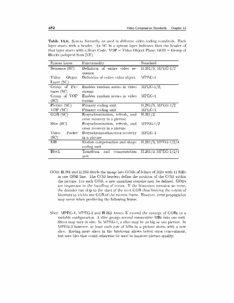
482 Video Compression Standards Chapter 13
Table 13.6. Syntax hierarchy as used in di�erent video coding standards. Each
layer starts with a header. An SC in a syntax layer indicates that the header of
that layer starts with a Start Code. VOP = Video Object Plane, GOB = Group of
Blocks (adapted from [13]).
Syntax Layer Functionality Standard
Sequence (SC) De�nition of entire video se-
quence
H.261/3, MPEG-1/2
Video Object
Layer (SC)
De�nition of entire video object MPEG-4
Group of Pic-
tures (SC)
Enables random access in video
stream
MPEG-1/2;
Group of VOP
(SC)
Enables random access in video
stream
MPEG-4
Picture (SC) Primary coding unit H.261/3, MPEG-1/2
VOP (SC) Primary coding unit MPEG-4
GOB (SC) Resynchronization, refresh, and
error recovery in a picture
H.261/3
Slice (SC) Resynchronization, refresh, and
error recovery in a picture
MPEG-1/2
Video Packet
(SC)
Resynchronization error recovery
in a picture
MPEG-4
MB Motion compensation and shape
coding unit
H.261/3, MPEG-1/2/4
Block Transform and compensation
unit
H.261/3, MPEG-1/2/4
GOB: H.261 and H.263 divide the image into GOBs of 3 lines of MBs with 11 MBs
in one GOB line. The GOB headers de�ne the position of the GOB within
the picture. For each GOB, a new quantizer stepsize may be de�ned. GOBs
are important in the handling of errors. If the bitstream contains an error,
the decoder can skip to the start of the next GOB thus limiting the extent of
biterrors to within one GOB of the current frame. However, error propagation
may occur when predicting the following frame.
Slice: MPEG-1, MPEG-2 and H.263 Annex K extend the concept of GOBs to a
variable con�guration. A slice groups several consecutive MBs into one unit.
Slices may vary in size. In MPEG-1, a slice may be as big as one picture. In
MPEG-2 however, at least each row of MBs in a picture starts with a new
slice. Having more slices in the bitstream allows better error concealment,
but uses bits that could otherwise be used to improve picture quality.
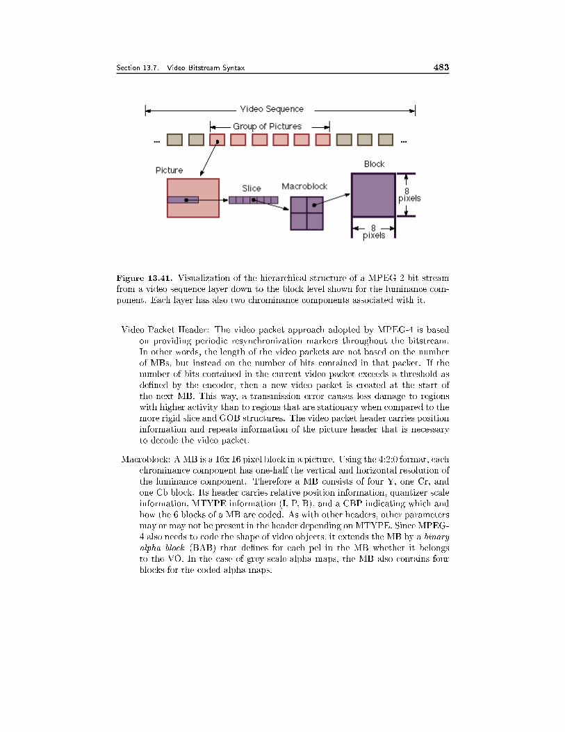
Section 13.7. Video Bitstream Syntax 483
Figure 13.41. Visualization of the hierarchical structure of a MPEG-2 bit stream
from a video sequence layer down to the block level shown for the luminance com-
ponent. Each layer has also two chrominance components associated with it.
Video Packet Header: The video packet approach adopted by MPEG-4 is based
on providing periodic resynchronization markers throughout the bitstream.
In other words, the length of the video packets are not based on the number
of MBs, but instead on the number of bits contained in that packet. If the
number of bits contained in the current video packet exceeds a threshold as
de�ned by the encoder, then a new video packet is created at the start of
the next MB. This way, a transmission error causes less damage to regions
with higher activity than to regions that are stationary when compared to the
more rigid slice and GOB structures. The video packet header carries position
information and repeats information of the picture header that is necessary
to decode the video packet.
Macroblock: A MB is a 16x 16 pixel block in a picture. Using the 4:2:0 format, each
chrominance component has one-half the vertical and horizontal resolution of
the luminance component. Therefore a MB consists of four Y, one Cr, and
one Cb block. Its header carries relative position information, quantizer scale
information, MTYPE information (I, P, B), and a CBP indicating which and
how the 6 blocks of a MB are coded. As with other headers, other parameters
may or may not be present in the header depending on MTYPE. Since MPEG-
4 also needs to code the shape of video objects, it extends the MB by a binary
alpha block (BAB) that de�nes for each pel in the MB whether it belongs
to the VO. In the case of grey-scale alpha maps, the MB also contains four
blocks for the coded alpha maps.
484 Video Compression Standards Chapter 13
Block: A block is the smallest coding unit in standardized video coding algorithms.
It consists of 8x8 pixels and can be one of three types: Y, Cr, or Cb. The pixels
of a block are represented by their DCT coeÆcients coded using a Hufman
code that codes the number of '0's before the next non-zero coeÆcient and
the amplitude of this coeÆcient.
The di�erent headers in the bitstream allow a decoder to recover from errors in
the bitstream and start decoding as soon as it receives a start code. The behaviour
of a decoder when receiving an erroneous bitstream is not de�ned in the standard.
Di�erent decoders may behave very di�erently, some decoders crash and require
rebooting of the terminal, others recover within a picture, yet others wait until the
next I-frame before they start decoding again.
13.8 Multimedia Content Description Using MPEG-7
With the ubiquitous use of video, the problem of indexing and searching for video
sequences becomes an important capability. MPEG-7 is an on-going standard-
ization e�ort for content description of audio-visual (AV) documents [32, 63]. In
principle, MPEG-1, -2, and -4 are designed to represent the information itself, while
MPEG-7 is meant to represent information about the information. Looking from
another perspective: MPEG-1/2/4 make content available, while MPEG-7 allows
you to �nd the content you need [63]. MPEG-7 is intended to provide complemen-
tary functionality to other MPEG standards: representing information about the
content, not the content itself (\the bits about the bits"). While MPEG-4 enables
to attach limited textual meta information to its streams, the MPEG-7 standard
will provide a full set of indexing and search capabilities such that we can search
for a movie not only with text keys but also with keys like color histograms, motion
trajectory, etc. MPEG-7 will be an international standard by the end of 2001.
In this section, we �rst provide an overview of the elements standardized by
MPEG-7. We then describe multimedia description schemes, with focus on con-
tent description. We explain how MPEG-7 decomposes an AV document to arrive
at both structural and semantic descriptions. Finally we describe visual descrip-
tors used in these descriptions. The descriptors and description schemes presented
below assume that semantically meaningful regions and objects can be segmented
and that the shape and motion parameters, and even semantic lables of these re-
gions/objects can be accurately extracted. We would like to note that generation
of such information remains an unsolved problem and may need manual assistance.
The MPEG-7 standard only de�nes the syntax that can be used to specify these
information, but not algorithms that can be used to extract them.
13.8.1 Overview
The main elements of the MPEG-7 standard are [32]:
� Descriptors (D): The MPEG-7 descriptors are designed to represent features,
Section 13.8. Multimedia Content Description Using MPEG-7 485
including low-level audio-visual features; high-level features of semantic ob-
jects, events and abstract concepts; information about the storage media,
and so on. Descriptors de�ne the syntax and the semantics of each feature
representation.
� Description Schemes (DS): The MPEG-7 DSs expand on the MPEG-7 de-
scriptors by combining individual descriptors as well as other DSs within more
complex structures and by de�ning the relationships among the constituent
descriptors and DSs.
� A Description De�nition Language (DDL): It is a language that allows the
creation of new DSs and, possibly, new descriptors. It also allows the exten-
sion and modi�cation of existing DSs. The XML Schema Language has been
selected to provide the basis for the DDL.
� System tools: These are tools that are needed to prepare MPEG-7 descrip-
tions for eÆcient transport and storage, and to allow synchronization between
content and descriptions, and to manage and protect intellectual property.
13.8.2 Multimedia Description Schemes
In MPEG-7, the DSs are categorized as pertaining speci�cally to the audio or visual
domain, or pertaining generically to the description of multimedia. The multime-
dia DSs are grouped into the following categories according to their functionality
(Fig. 13.42):
� Basic elements: These deal with basic datatypes, mathematical structures,
schema tools, linking and media localization tools as well as basic DSs, which
are elementary components of more complex DSs;
� Content description: These DSs describe the structural and conceptual as-
pects of an AV document;
� Content management: These tools specify information about the storage me-
dia, the creation and the usage of an AV document;
� Content organization: These tools address the organization of the content
by classi�cation, by the de�nition of collections of AV documents, and by
modeling;
� Navigation and access: These include summaries for browsing and variations
of the same AV content for adaptation to capabilities of the client terminals,
network conditions or user preferences;
� User interaction: These DSs specify user preferences pertaining to the con-
sumption of the multimedia material.
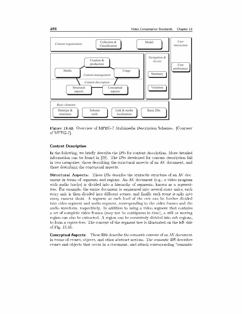
486 Video Compression Standards Chapter 13
Datatype &
structures
Link & media
localization
Basic DSs
Model
Basic elements
Navigation &
Access
Content management
Content description
Collection &
Classification
Summary
Variation
Content organization
Creation &
production
Media Usage
Conceptual
aspects
Structural
aspects
User
interaction
User
preferences
Schema
tools
Figure 13.42. Overview of MPEG-7 Multimedia Description Schemes. [Courtesy
of MPEG-7].
Content Description
In the following, we brie y describe the DSs for content description. More detailed
information can be found in [29]. The DSs developed for content description fall
in two categories: those describing the structural aspects of an AV document, and
those describing the conceptual aspects.
Structural Aspects: These DSs describe the syntactic structure of an AV doc-
ument in terms of segments and regions. An AV document (e.g., a video program
with audio tracks) is divided into a hierarchy of segments, known as a segment-
tree. For example, the entire document is segmented into several story units, each
story unit is then divided into di�erent scenes, and �nally each scene is split into
many camera shots. A segment at each level of the tree can be further divided
into video segment and audio segment, corresponding to the video frames and the
audio waveform, respectively. In addition to using a video segment that contains
a set of complete video frames (may not be contiguous in time), a still or moving
region can also be extracted. A region can be recursively divided into sub-regions,
to form a region-tree. The concept of the segment tree is illustrated on the left side
of Fig. 13.43.
Conceptual Aspects: These DSs describe the semantic content of an AV document
in terms of events, objects, and other abstract notions. The semantic DS describes
events and objects that occur in a document, and attach corresponding \semantic
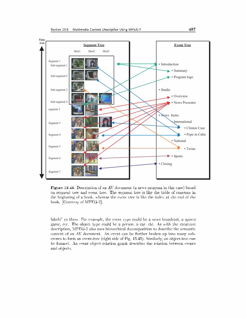
Section 13.8. Multimedia Content Description Using MPEG-7 487
Segment Tree
Shot1 Shot2 Shot3
Segment 1 Sub-segment 1
Sub-segment 2
Sub-segment 3
Sub-segment 4
segment 2
Segment 3
Segment 4
Segment 5
Segment 6
Segment 7
Event Tree
• Introduction
• Summary
• Program logo
• Studio
• Overview
• News Presenter
• News Items
• International
• Clinton Case
• Pope in Cuba
• National
• Twins
• Sports
• Closing
Time Axis
Figure 13.43. Description of an AV document (a news program in this case) based
on segment tree and event tree. The segment tree is like the table of contents in
the beginning of a book, whereas the event tree is like the index at the end of the
book. [Courtesy of MPEG-7].
labels" to them. For example, the event type could be a news broadcast, a sports
game, etc. The object type could be a person, a car, etc. As with the structure
description, MPEG-7 also uses hierarchical decomposition to describe the semantic
content of an AV document. An event can be further broken up into many sub-
events to form an event-tree (right side of Fig. 13.43). Similarly, an object-tree can
be formed. An event-object relation graph describes the relation between events
and objects.
488 Video Compression Standards Chapter 13
Relation between Structure and Semantic DSs: An event is usually associated
with a segment, and an object with a region. Each event or object may occur
multiple times in a document, and their actual locations (which segment or region)
are described by a set of links, as shown in Fig. 13.43. In this sense, the syntactic
structure, represented by the segment-tree and the region-tree, is like the table of
contents in the beginning of a book, whereas the semantic structure, i.e., the event-
tree and the object-tree, is like the index at the end of the book.
13.8.3 Visual Descriptors and Description Schemes
For each segment or region at any level of the segment- or region-tree, a set of audio
and visual descriptors and DSs are used to characterize this segment or region. In
this section, we brie y describe the visual descriptors and DSs that have been
developed to describe the color, texture, shape, motion, and location of a video
segment or object. More complete descriptions can be found in [28, 33].
Color
These descriptors describe the color distributions in a video segment, a moving
region or a still region.
� Color space: Five color spaces are de�ned, RGB, YCrCb, HSV, HMMD, or
monochrome. Alternatively, one can specify an arbitrary linear transformation
matrix from the RGB coordinate.
� Color quantization: This descriptor is used to specify the quantization pa-
rameters, including the number of quantization levels and starting values for
each color component. Only uniform quantization is considered.
� Dominant color: This descriptor speci�es the dominant colors in the underly-
ing segment, including the number of dominant colors, a value indicating the
spatial coherence of the dominant color (i.e., whether the dominant color is
scattered over the segment or form a cluster), and for each dominant color,
the percentage of pixels taking that color, the color value and its variance.
� Color histogram: The color histogram is de�ned in the HSV space. Instead of
the color histogram itself, the Haar transform is applied to the histogram and
the Haar coeÆcients are speci�ed using variable precision depending on the
available bit rate. Several types of histograms can be speci�ed. The common
color histogram, which includes the percentage of each quantized color among
all pixels in a segment or region, is called ScalableColor. The GoF/GoP Color
refers to the average, median, or intersection (minimum percentage for each
color) of conventional histograms over a group of frames or pictures.
� Color layout: This descriptor is used to describe in a coarse level the color
pattern of an image. An image is reduced to 8 � 8 blocks with each block
Section 13.8. Multimedia Content Description Using MPEG-7 489
represented by its dominant color. Each color component (Y/Cb/Cr) in the
reduced image is then transformed using DCT, and �rst few coeÆcients are
speci�ed.
� Color structure: This descriptor is intended to capture the spatial coherence
of pixels with the same color. The counter for a color is incremented as long
as there is at least one pixel with this color in a small neighborhood around
each pixel, called the structuring element. Unlike the color histogram, this
descriptor can distinguish between two images in which a given color is present
in identical amounts but where the structure of the groups of pixels having
that color is di�erent in the two images.
Texture
This category is used to describe the texture pattern of an image.
� Homogeneous texture: This is used to specify the energy distribution in di�er-
ent orientations and frequency bands (scales). The �rst two components are
the mean value and the standard deviation of the pixel intensities. The follow-
ing 30 components are obtained through a Gabor transform with 6 orientation
zones and 5 scale bands.
� Texture browsing: This descriptor speci�es the texture appearances in terms
of regularity, coarseness and directionality, which are in-line with the type of
descriptions that a human may use in browsing/retrieving a texture pattern.
In addition to regularity, up to two dominant directions and the coarseness
along each direction can be speci�ed.
� Edge histogram: This descriptor is used to describe the edge orientation dis-
tribution in an image. Three types of edge histograms can be speci�ed, each
with �ve entries, describing the percentages of directional edges in four pos-
sible orientations and non-directional edges. The global edge histogram is
accumulated over every pixel in an image; the local histogram consists of 16
sub-histograms, one for each block in an image divided into 4� 4 blocks; the
semi-global histogram consists of 13 sub-histograms, one for each sub-region
in an image.
Shape
These descriptors are used to describe the spatial geometry of still and moving
regions.
� Contour-based descriptor: This descriptor is applicable to a 2D region with
a closed boundary. MPEG-7 has chosen to use the peaks in the curvature
scale space (CSS) representation [55] to describe a boundary, which has been
found to re ect human perception of shapes, i.e., similar shapes have simi-
lar parameters in this representation. The CSS representation of a boundary
490 Video Compression Standards Chapter 13
is obtained by recursively blurring the original boundary using a smoothing
�lter, computing the curvature along each �ltered curve, and �nally deter-
mining zero-crossing locations of the curvature after successive blurring. The
descriptor speci�es the number of curvature peaks in the CSS, the global ec-
centricity and circularity of the boundary, the eccentricity and circularity of
the prototype curve, which is the curve leading to the highest peak in the
CSS, the prototype �lter, and the positions of the remaining peaks.
� Region-based shape descriptor: The region-based shape descriptor makes use
of all pixels constituting the shape, and thus can describe any shape, i.e. not
only a simple shape with a single connected region but also a complex shape
that consists of several disjoint regions. Speci�cally, the original shape repre-
sented by an alpha map is projected onto Angular Radial Transform (ART)
basis functions, and the descriptor includes 35 normalized and quantized mag-
nitudes of the ART coeÆcients.
� Shape 3D: This descriptor provides an intrinsic description of 3D mesh models.
It exploits some local attributes of the 3D surface. To derive this descriptor,
the so-called shape index is calculated at every point on the mesh surface,
which depends on the principle curvature at the point. The descriptor speci�es
the shape spectrum, which is the histogram of the shape indices calculated
over the entire mesh. Each entry in the histogram essentially speci�es the
relative area of all the 3D mesh surface regions with a shape index lying in
a particular interval. In addition, the descriptor includes the relative area of
planar surface regions of the mesh, for which the shape index is not de�ned,
and the relative area of all the singular polygonal components, which are
regions for which reliable estimation of the shape index is not possible.
Motion
These descriptors describe the motion characteristics of a video segment or a moving
region as well as global camera motion.
� Camera motion: Seven possible camera motions are considered: panning,
tracking (horizontal translation), tilting, booming (vertical translation), zoom-
ing, dollying (translation along the optical axis), and rolling (rotation around
the optical axis) (cf. Fig. 5.4). For each motion, two moving directions are
possible. For each motion type and direction, the presence (i.e. duration),
speed and the amount of motion are speci�ed. The last term measures the
area that is covered or uncovered due to a particular motion.
� Motion trajectory: This descriptor is used to specify the trajectory of a non-
rigid moving object, in terms of the 2D or 3D coordinates of certain key points
at selected sampling times. For each key point, the trajectory between two
adjacent sampling times is interpolated by a speci�ed interpolation function
(either linear or parabolic).
Section 13.9. Summary 491
� Parametric object motion: This descriptor is used to specify the 2D motion
of a rigid moving object. Five types of motion models are included: transla-
tion, rotation/scaling, aÆne, planar perspective, and parabolic. The planar
perspective and parabolic motions refer to the projective mapping de�ned in
Eq. 5.5.14, and the biquadratic mapping de�ned in Eq. 5.5.19, respectively.
In addition to the model type and model parameters, the coordinate origin
and time duration need to be speci�ed.
� Motion activity: This descriptor is used to describe the intensity and spread
of activity over a video segment (typically at the shot level). Four attributes
can be speci�ed: i) intensity of activity, measured by the standard deviation
of the motion vector magnitudes; ii) direction of activity, which speci�es the
dominant or average direction of all motion vectors; iii) spatial distribution
of activity, derived from the run-lengths of blocks with motion magnitudes
lower than the average magnitude, iv) spatial localization of activity, and
v) temporal distribution of activity, described by a histogram of quantized
activity levels over individual frames in the shot.
Localization
These descriptors and DSs are used to describe the location of a still or moving
region.
� Region locator: This descriptor speci�es the location of a region by a brief
and scalable representation of a bounding box or polygon.
� Spatial-temporal locator: This DS describes a moving region. It decomposes
the entire duration of the region into a few sub-segments, with each segment
being speci�ed by the shape of the region in the beginning of the segment,
known as a reference region, and the motion between this region and the ref-
erence region of the next segment. For a non-rigid object, a FigureTrajectory
DS is developed, which de�nes the reference region by a bounding rectangle,
ellipse, or polygon, and speci�es the motion between reference regions using
the MotionTrajectory descriptor, which speci�es the coordinates of selected
key points over successive sampling times. For a rigid region, a Parameter-
Trajectory DS is used, which uses the RegionLocator descriptor to specify a
reference region, and the parametric object motion descriptor to describe the
motion.
13.9 Summary
Video communications requires standardization in order to build reasonably-priced
equipment that interoperates and caters to a large market. Personal video telephony
was the �rst application that was targeted by a digital video compression standard.
H.261 was published in 1990, 101 years after Jules Vernes wrote down the idea of
492 Video Compression Standards Chapter 13
a video telephone and 899 years earlier than he predicted [68]. The subsequent
important video compression standards H.263, MPEG-1, MPEG-2, and MPEG-4
were established in 1993, 1995, 1995, and 1999, respectively.
Whereas the H.261 and H.263 standards describe only video compression, MPEG-
1/2/4 standards describe also the representation of audio as well as a system that
enables the joint transmission of audiovisual signals. H.261 is a block-based hybrid
coder with integer-pel motion compensation. The main applications for H.261 is
video coding for video conferencing over ISDN lines at rates between 64 kbit/s and
2 Mbit/s. H.263 extends H.261 and adds many features including half-pel motion
compensation thus enabling video coding for transmission over analog telephone
lines at rates below 56 kbit/s.
MPEG-1 is also derived from H.261. It added half-pel motion compensation,
bidirectional prediction for B-pictures and other improvements in order to meet the
requirements for coding video at rates around 1.2 Mbit/s for consumer video on
CD-ROM at CIF resolution. MPEG-2 is the �rst standard that is able to code
interlaced video at full TV and HDTV resolution. It extended MPEG-1 to include
new prediction modes for interlaced video. Its main applications are TV broadcast-
ing at rates around 4 Mbit/s and 15 Mbit/s for high-quality video. MPEG-4 video,
based on MPEG-2 and H.263, is the latest video coding standard that introduces
object-based functionalities describing video objects not only with motion and tex-
ture but also by their shape. Shape information is co-located with the luminance
signal and coded using a context-based arithmetic coder.
MPEG-2 and MPEG-4 de�ne pro�les that require a decoder to implement a sub-
set of the tools that the standard de�nes. This enables to build standard decoders
that are to some extend taylored towards certain application areas.
Whereas MPEG-1/2/4 standards are developed to enable the exchange of au-
diovisual data, MPEG-7 aims to enable the searching and browsing of such data.
MPEG-7 can be used independent of the other MPEG standards | an MPEG-7
description might even be attached to an analog movie. MPEG-7 descriptions could
be used to improve the functionalities of previous MPEG standards, but will not
replace MPEG-1, MPEG-2 or MPEG-4.
Since the computational power in terminals increases every year, standardization
bodies try to improve on their standards. ITU currently works on the video coding
standard H.26L that promises to outperform H.263 and MPEG-4 by more than
1 dB for the same bitrate or reducing the bitrate by more than 20% for the same
picture quality when coding video at rates above 128 kbit/s.
13.10 Problems
13.1 What kinds of compatibility do you know?
13.2 What are the most compute intensive parts of an H.261 video encoder. What
are the most compute intensive parts of a decoder?
Section 13.10. Problems 493
13.3 What is a loop �lter? Why is H.261 the only standard implementing it?
13.4 What are the tools that improve the coding eÆciency of H.263 over H.261?
13.5 What is the main di�erence between MPEG-1 B-frames and H.263 PB-frames
according to the Improved PB-frame mode?
13.6 What is the purpose of the standards H.323 and H.324?
13.7 Why does MPEG-2 have more than one scan mode?
13.8 What e�ect does the perceptual quantization of I frames have on the PSNR
of a coded picture? How does perceptual quantization a�ect picture quality.
What is a good guideline for choosing the coeÆcients of the weight matrix?
13.9 Explain the concept of pro�les and levels in MPEG-2.
13.10 Which of the MPEG-2 pro�les are used in commercial products? Why do
the others exist?
13.11 What kind of scalability is supported by MPEG-2?
13.12 What is drift? When does it occur?
13.13 Discuss the error resilience tools that H.261, H.263, MPEG-1/2/4 provide?
Why are MPEG-4 error resilience tools best suited for lossy transmission chan-
nels?
13.14 What are the di�erences between MPEG-1 Layer III audio coding andMPEG-
2 NBC audio?
13.15 MPEG-4 allows to encode shape signals. In case of binary shape, how many
blocks are associated with a macroblock? What is their size? What about
greyscale shape coding?
13.16 Why does MPEG-4 video according to the ACE pro�le outperform MPEG-1
video?
13.17 What part of an MPEG-4 terminal is not standardized?
13.18 Why do video bitstreams contain start codes?
13.19 What is meta information?
13.20 Which standard uses a wavelet coder and for what purpose?
13.21 Why is the de�nition of FAP's as done in MPEG-4 important for content
creation?
494 Video Compression Standards Chapter 13
13.22 How is synchronization achieved between a speech synthesizer and a talking
face?
13.23 What is the functionality and purpose of MPEG-4 mesh animation?
13.24 What is the diÆculty with video indexing and retrieval? How can a standard-
ized content description interface such as MPEG-7 simplify video retrieval?
13.25 How does the segment-tree in MPEG-7 describe the syntactic structure of a
video sequence? How does the event-tree in MPEG-7 describe the semantic
structure of a video sequence? What are their relations?
13.26 What are the visual descriptors developed by MPEG-7? Assuming these
descriptors are attached to every video sequence in a large video database.
Describe ways that you may use them to retrieve certain type of sequences.
13.11 Bibliography
[1] O. Avaro, A. Elftheriadis, C. Herpel, G. Rajan, and L. Ward. MPEG-4 systems:
Overview. In A. Puri and T. Chen, editors, Multimedia Systems, Standards, and
Networks. Marcel Dekker, 2000.
[2] A. Basso, M. R. Civanlar, and V. Balabanian. Delivery and control of MPEG-4
content over IP networks. In A. Puri and T. Chen, editors, Multimedia Systems,
Standards, and Networks. Marcel Dekker, 2000.
[3] K. Brandenburg, O. Kunz, and A. Sugiyama. MPEG-4 natural audio coding.
Signal Processing: Image Communication, 15(4-5):423{444, 2000.
[4] T. K. Capin, E. Petajan, and J. Ostermann. EÆcient modeling of virtual humans
in MPEG-4. In Proceedings of the International Conference on Multimedia and
Expo 2000, page TPS9.1, New York, 2000.
[5] T. Chen. Emerging standards for multimedia applications. In L. Guan, S. Y.
Kung, and J. Larsen, editors, Multimedia Image and Video Processing, pages 1{18.
CRC Press, 2000.
[6] T. Chen, G. J. Sullivan, and A. Puri. H.263 (including H.263++) and other ITU-
T video coding standards. In A. Puri and T. Chen, editors, Multimedia Systems,
Standards, and Networks. Marcel Dekker, 2000.
[7] L. Chiariglione. Communication standards: G�otterd�ammerung? In A. Puri
and T. Chen, editors, Multimedia Systems, Standards, and Networks, pages 1{22.
Marcel Dekker, 2000.
[8] F. Dufaux and F. Moscheni. Motion estimation techniques for digital TV: A
review and a new contribution. Proceedings of the IEEE, 83(6):858{876, June 1995.
Section 13.11. Bibliography 495
[9] Y. Lee E. D. Scheirer and J.-W. Yang. Synthetic and snhc audio in MPEG-4.
Signal Processing: Image Communication, 15(4-5):445{461, 2000.
[10] B. Girod, E. Steinbach, and N. F�arber. Comparison of the H.263 and H.261
video compression standards. In Standards and Common Interfaces for Video,
Philadelphia, USA, October 1995. SPIE Proceedings Vol. CR60, SPIE.
[11] J. Hartman and J. Wernecke. The VRML handbook. Addison Wesley, 1996.
[12] B. G. Haskell, P. G. Howard, Y. A. LeCun, A. Puri, J. Ostermann, M. R.
Civanlar, L. Rabiner, L. Bottou, and P. Ha�ner. Image and video codingemerging
standards and beyond. IEEE Transactions on Circuits and Systems for Video
Technology, 8(7):814{837, November 1998.
[13] B. G. Haskell, A. Puri, and A. N. Netravali. Digital Video: An Introduction to
MPEG-2. Chapman & Hall, New York, 1997.
[14] C. Herpel, A. Elftheriadis, and G. Franceschini. MPEG-4 systems: Elementary
stream management and delivery. In A. Puri and T. Chen, editors, Multimedia
Systems, Standards, and Networks. Marcel Dekker, 2000.
[15] ISO/IEC. IS 10918-1: Information technology { digital compression and coding
of continuous-tone still images: Requirements and guidelines, 1990. (JPEG).
[16] ISO/IEC. IS 11172: Information technology { Coding of moving pictures and
associated audio for digital storage media at up to about 1.5 mbit/s, 1993. (MPEG-
1).
[17] ISO/IEC. IS 13818-2: Information technology { Generic coding of moving
pictures and associated audio information: Video, 1995. (MPEG-2 Video).
[18] ISO/IEC. IS 13818-3: Information technology { Generic coding of moving
pictures and associated audio information { part 3: Audio, 1995. (MPEG-2 Audio).
[19] ISO/IEC. IS 13818: Information technology { Generic coding of moving pic-
tures and associated audio information: Systems, 1995. (MPEG-2 Systems).
[20] ISO/IEC. IS 13818-3: Information technology { Generic coding of moving
pictures and associated audio information { part 7: Advanced audio coding (AAC),
1997. (MPEG-2 AAC).
[21] ISO/IEC. IS 14772-1: Information technology - computer graphics and image
processing - the virtual reality modeling language - part 1: Functional speci�cation
and UTF-8 encoding, 1997. (VRML).
[22] ISO/IEC. IS 14496: Information technology { coding of audio-visual objects,
1999. (MPEG-4).
496 Video Compression Standards Chapter 13
[23] ISO/IEC. IS 14496: Information technology { coding of audio-visual objects {
part 1: Systems, 1999. (MPEG-4 Systems).
[24] ISO/IEC. IS 14496: Information technology { coding of audio-visual objects {
part 2: Visual, 1999. (MPEG-4 Video).
[25] ISO/IEC. IS 16500: Information technology { generic digital audio-visual
systems, 1999. (DAVIC).
[26] ISO/IEC. Report of the formal veri�cation tests on advanced coding eÆciency
ACE (formerly Main Plus) pro�le in version 2. Public document, ISO/IEC JTC
1/SC 29/WG 11 N2824, July 1999.
[27] ISO/IEC. Report of the formal veri�cation tests on mpeg-4 coding eÆciency
for low and medium bit rates. Public document, ISO/IEC JTC 1/SC 29/WG 11
N2826, July 1999.
[28] ISO/IEC. CD 15938-3: MPEG-7 multimedia content description interface -
part 3: Visual. Public document, ISO/IEC JTC1/SC29/WG11 W3703, La Baule,
October 2000.
[29] ISO/IEC. CD 15938-5: information technology - multimedia content de-
scription interface - part 5: Multimedia description schemes. Public document,
ISO/IEC JTC1/SC29/WG11 N3705, La Baule, October 2000.
[30] ISO/IEC. IS 14496: Information technology { coding of audio-visual objects {
part 3: Audio, 2000. (MPEG-4 Audio).
[31] ISO/IEC. IS 14496: Information technology { coding of audio-visual objects
{ part 6: Delivery multimedia integration framework (DMIF), 2000. (MPEG-4
DMIF).
[32] ISO/IEC. Overview of the MPEG-7 standard (version 4.0). Public document,
ISO/IEC JTC1/SC29/WG11 N3752, La Baule, October 2000.
[33] ISO/IEC. MPEG-7 visual part of eXperimentation Model Version 9.0. Public
document, ISO/IEC JTC1/SC29/WG11 N3914, Pisa, January 2001.
[34] ITU-R. BT.601-5: Studio encoding parameters of digital television for standard
4:3 and wide-screen 16:9 aspect ratios, 1998. (Formerly CCIR 601).
[35] ITU-T. Recommendation G.711: Pulse code modulation (PCM) of voice fre-
quencies, 1988.
[36] ITU-T. Recommendation G.722: 7 kHz audio-coding within 64 kbit/s, 1988.
[37] ITU-T. Recommendation G.723.1: Dual rate speech coder for multimedia
communications transmitting at 5.3 and 6.3 kbit/s, 1988.
Section 13.11. Bibliography 497
[38] ITU-T. Recommendation G.728: Coding of speech at 16 kbit/s using low-delay
code excited linear prediction, 1992.
[39] ITU-T. Recommendation T.81 - Information technology - Digital compression
and coding of continuous-tone still images - Requirements and guidelines, 1992.
(JPEG).
[40] ITU-T. Recommendation H.261: Video codec for audiovisual services at px64
kbits, 1993.
[41] ITU-T. Recommendation V.34: A modem operating at data signaling rates of
up to 28,800 bit/s for use on the general switched telephone network and on leased
point-to-point 2-wire telephone-type circuits, 1994.
[42] ITU-T. Recommendation H.262: Information technology - generic coding of
moving pictures and associated audio information: Video, 1995.
[43] ITU-T. Recommendation H.324: Terminal for low bitrate multimedia commu-
nication, 1995.
[44] ITU-T. Recommendation H.223: Multiplexing protocol for low bit rate multi-
media communication, 1996.
[45] ITU-T. Recommendation H.320: Narrow-band visual telephone systems and
terminal equipment, 1997.
[46] ITU-T. Recommendation V.25ter: Serial asynchronous automatic dialling and
control, 1997.
[47] ITU-T. Recommendation H.225.0: Call signaling protocols and media stream
packetization for packet based multimedia communications systems, 1998.
[48] ITU-T. Recommendation H.245: Control protocol for multimedia communica-
tion, 1998.
[49] ITU-T. Recommendation H.263: Video coding for low bit rate communication,
1998.
[50] ITU-T. Recommendation H.323: Packet-based multimedia communciations
systems, 1998.
[51] ITU-T. Recommendation V.8 bis: Procedures for the identi�cation and selec-
tion of common modes of operation between data circuit- terminating equipments
(DCEs) and between data terminal equipments (DTEs) over the public switched
telephone network and on leased point-to-point telephone-type circuits, 1998.
[52] ITU-T. Recommendation V.8: Procedures for starting sessions of data trans-
mission over the public switched telephone network, 1998.
498 Video Compression Standards Chapter 13
[53] R. Koenen. Pro�les and levels in MPEG-4: approach and overview. Signal
Processing: Image Communications, 15(4-5):463{478, 2000.
[54] J. L. Mitchell, W. B. Pennebaker, C. E. Fogg, and D. J. LeGall. MPEG video
compression standard. Digital Multimedia Standards Series. Chapman and Hall,
Bonn, 1996.
[55] F.S. Mokhtarian, S. Abbasi, and J. Kittler. Robust and eÆcient shape indexing
through curvature scale space. In British Machine Vision Conference, pages 53{62,
Edinburgh, UK, 1996.
[56] H. G. Musmann and J. Klie. TV transmission using a 64 kbit/s transmission
rate. In International Conference on Communications, pages 23.3.1{23.3.5, 1979.
[57] S. Okubo. Reference model methodology - a tool for the collaborative creation
of video coding standards. Proceedings of the IEEE, 83(2):139{150, February 1995.
[58] M. T. Orchard and G. J. Sullivan. Overlapped block motion compensation:
An estimation-theoretic approach. IEEE Trans. Image Process., 3:693{699, 1994.
[59] J. Ostermann and A. Puri. Natural and synthetic video in MPEG-4. In Proceed-
ings of the International Conference on Acoustics, Speech and Signal Processing
(ICASSP), pages 3805{3809, November 1998.
[60] A. Puri. Video coding using the MPEG-2 compression standard. In SPIE Vi-
sual communications and image processing, volume 1199, pages 1701{1713, Novem-
ber 1993.
[61] A. Puri and A. Wong. Spatial domain resolution scalable video coding. In
SPIE Visual communications and image processing, volume 1199, pages 718{729,
November 1993.
[62] A. Puri, L. Yan, and B. G. Haskell. Temporal resolution scalable video coding.
In International conference on image processing (ICIP 94), volume 2, pages 947{
951, November 1994.
[63] P. Salembier and J. R. Smith. MPEG-7 multimedia description schemes. IEEE
Trans. Circuits and Systems for Video Technology, 2001, to appear.
[64] H. Schulzrinne, S. Casner, R. Frederick, and V. Jacobson. RTP: A trans-
port protocol for real-time applications. RFC 1889, IETF, available from
ftp://ftp.isi.edu/in-notes/rfc1889.txt, January 1996.
[65] J. Signes, Y. Fisher, and A. Eleftheriadis. MPEG-4's binary format for scene
description. Signal Processing: Image Communication, 15(4-5):321{345, 2000.
[66] J. Sign�es, Y. Fisher, and A. Elftheriadis. MPEG-4: Scene representation and
interactivity. In A. Puri and T. Chen, editors, Multimedia Systems, Standards,
and Networks. Marcel Dekker, 2000.
Section 13.11. Bibliography 499
[67] A. M. Tekalp and J. Ostermann. Face and 2-D mesh animation in MPEG-4.
Signal Processing: Image Communication, Special Issue on MPEG-4, 15:387{421,
January 2000.
[68] J. Vernes. In the twenty-ninth century. The day of an American journalist in
2889. In Yesterday and Tomorrow, pages 107{124, London, 1965. Arco. Translated
from French, orignal text 1889.
[69] T. Wiegand, M. Lightstone, D. Mukherjee, T. Campell, and S. K. Mitra.
Rate-distortion optimized mode selection for very low bit rate video coding and
the emerging H.263 standard. IEEE Trans. Circuits Syst. for Video Technology,
6(2):182{190, Apr. 1996.
Chapter 14
ERROR CONTROL IN VIDEO
COMMUNICATIONS
We have discussed various video coding techniques and standards in previous chap-
ters. For e�ective video communications, reduction of raw video data rates is only
one of the necessary steps. Another equally important task is how to handle errors
and losses in a communication network. In contrast with data communications,
which are not usually subject to strict delay constraints and can therefore be han-
dled using network protocols that use retransmission to ensure error-free delivery,
real-time video is delay sensitive and cannot easily make use of retransmission. The
extensive use of predictive coding and variable length coding (VLC) in video coding
renders compressed video especially vulnerable to transmission errors, and success-
ful video communication in the presence of errors requires careful designs of the
encoder, decoder, and other system layers.
In this chapter, we present approaches that have been developed for error control
in video communications. We start by describing the necessity and the challenges
in error control for video communications and providing an overview of various
approaches that have been developed (Sec. 14.1). To help understand the issues
in error control in video communications, we describe in Sec. 14.2 the QoS re-
quirements of various video services and characteristics of di�erent networks. Sec-
tion 14.3 presents error control mechanisms at the transport level. Sections 14.4 and
14.5 review techniques for error-resilient encoding and error concealment. Finally,
Sec. 14.6 describes techniques that rely on encoder and decoder interactions. Fi-
nally, Sec. 14.7 summarizes error resilience tools adopted by the H.263 and MPEG-4
standards.
14.1 Motivation and Overview of Approaches
A video communication system typically involves �ve steps, as shown in Fig. 14.1.
The video is �rst compressed by a video encoder to reduce the data rate and the
compressed bit stream is then segmented into �xed or variable length packets and
multiplexed with other data types, such as audio. The packets might be sent directly
500
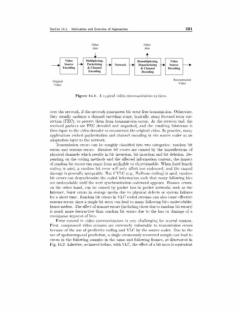
Section 14.1. Motivation and Overview of Approaches 501
Multiplexing,
Packetizing
& Channel
Encoding
Network
Demultiplexing,
Depacketizing
& Channel
Decoding
Video
Source
Encoding
Video
Source
Decoding
Original
Video
Reconstructed
Video
Other
data
Other
data
Figure 14.1. A typical video communication system.
over the network, if the network guarantees bit error free transmission. Otherwise,
they usually undergo a channel encoding stage, typically using forward error cor-
rection (FEC), to protect them from transmission errors. At the receiver end, the
received packets are FEC decoded and unpacked, and the resulting bitstream is
then input to the video decoder to reconstruct the original video. In practice, many
applications embed packetization and channel encoding in the source coder as an
adaptation layer to the network.
Transmission errors can be roughly classi�ed into two categories: random bit
errors and erasure errors. Random bit errors are caused by the imperfections of
physical channels which results in bit inversion, bit insertion and bit deletion. De-
pending on the coding methods and the a�ected information content, the impact
of random bit errors can range from negligible to objectionable. When �xed length
coding is used, a random bit error will only a�ect one codeword, and the caused
damage is generally acceptable. But if VLC (e.g., Hu�man coding) is used, random
bit errors can desynchronize the coded information such that many following bits
are undecodable until the next synchronization codeword appears. Erasure errors,
on the other hand, can be caused by packet loss in packet networks such as the
Internet, burst errors in storage media due to physical defects or system failures
for a short time. Random bit errors in VLC coded streams can also cause e�ective
erasure errors since a single bit error can lead to many following bits undecodable,
hence useless. The e�ect of erasure errors (including those due to random bit errors)
is much more destructive than random bit errors due to the loss or damage of a
contiguous segment of bits.
Error control in video communications is very challenging for several reasons.
First, compressed video streams are extremely vulnerable to transmission errors
because of the use of predictive coding and VLC by the source coder. Due to the
use of spatiotemporal prediction, a single erroneously recovered sample can lead to
errors in the following samples in the same and following frames, as illustrated in
Fig. 14.2. Likewise, as hinted before, with VLC, the e�ect of a bit error is equivalent
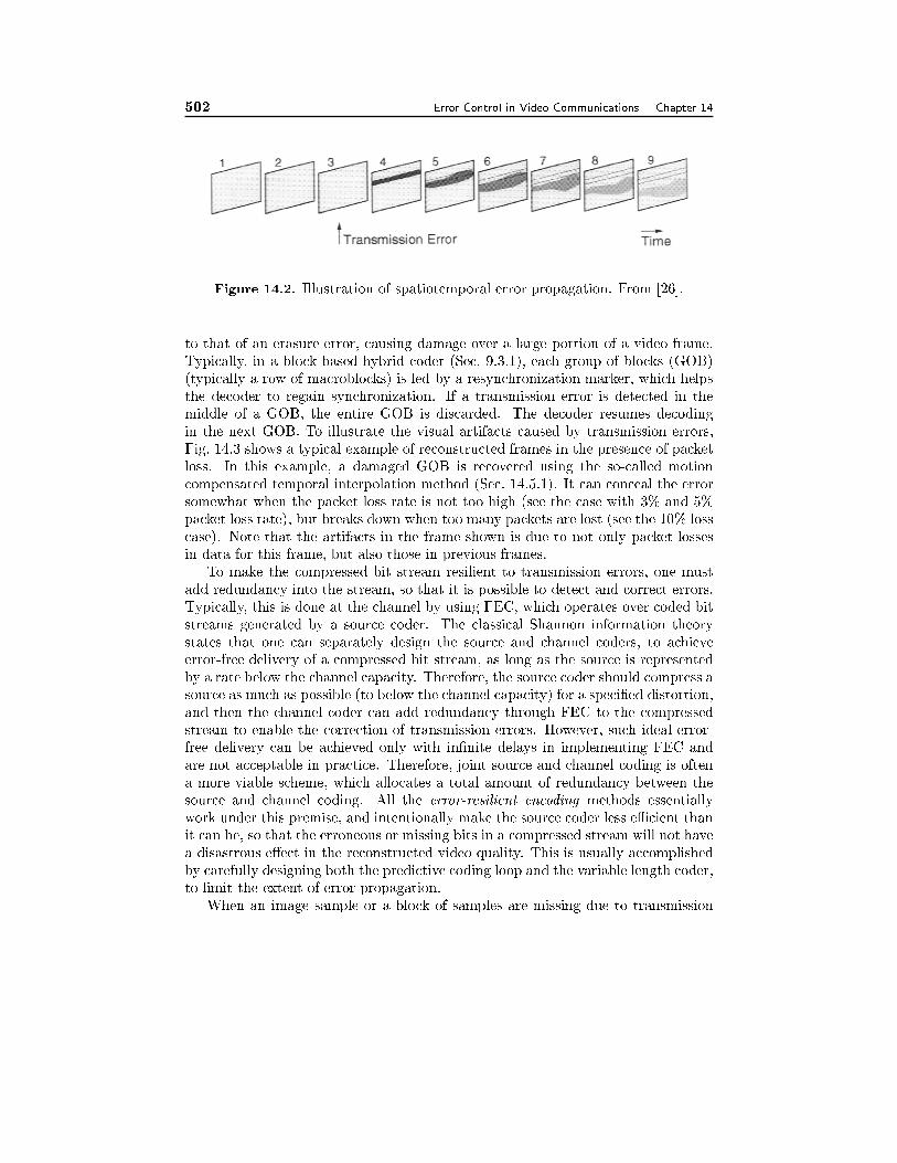
502 Error Control in Video Communications Chapter 14
Figure 14.2. Illustration of spatiotemporal error propagation. From [26].
to that of an erasure error, causing damage over a large portion of a video frame.
Typically, in a block-based hybrid coder (Sec. 9.3.1), each group of blocks (GOB)
(typically a row of macroblocks) is led by a resynchronization marker, which helps
the decoder to regain synchronization. If a transmission error is detected in the
middle of a GOB, the entire GOB is discarded. The decoder resumes decoding
in the next GOB. To illustrate the visual artifacts caused by transmission errors,
Fig. 14.3 shows a typical example of reconstructed frames in the presence of packet
loss. In this example, a damaged GOB is recovered using the so-called motion
compensated temporal interpolation method (Sec. 14.5.1). It can conceal the error
somewhat when the packet loss rate is not too high (see the case with 3% and 5%
packet loss rate), but breaks down when too many packets are lost (see the 10% loss
case). Note that the artifacts in the frame shown is due to not only packet losses
in data for this frame, but also those in previous frames.
To make the compressed bit stream resilient to transmission errors, one must
add redundancy into the stream, so that it is possible to detect and correct errors.
Typically, this is done at the channel by using FEC, which operates over coded bit
streams generated by a source coder. The classical Shannon information theory
states that one can separately design the source and channel coders, to achieve
error-free delivery of a compressed bit stream, as long as the source is represented
by a rate below the channel capacity. Therefore, the source coder should compress a
source as much as possible (to below the channel capacity) for a speci�ed distortion,
and then the channel coder can add redundancy through FEC to the compressed
stream to enable the correction of transmission errors. However, such ideal error-
free delivery can be achieved only with in�nite delays in implementing FEC and
are not acceptable in practice. Therefore, joint source and channel coding is often
a more viable scheme, which allocates a total amount of redundancy between the
source and channel coding. All the error-resilient encoding methods essentially
work under this premise, and intentionally make the source coder less eÆcient than
it can be, so that the erroneous or missing bits in a compressed stream will not have
a disastrous e�ect in the reconstructed video quality. This is usually accomplished
by carefully designing both the predictive coding loop and the variable length coder,
to limit the extent of error propagation.
When an image sample or a block of samples are missing due to transmission
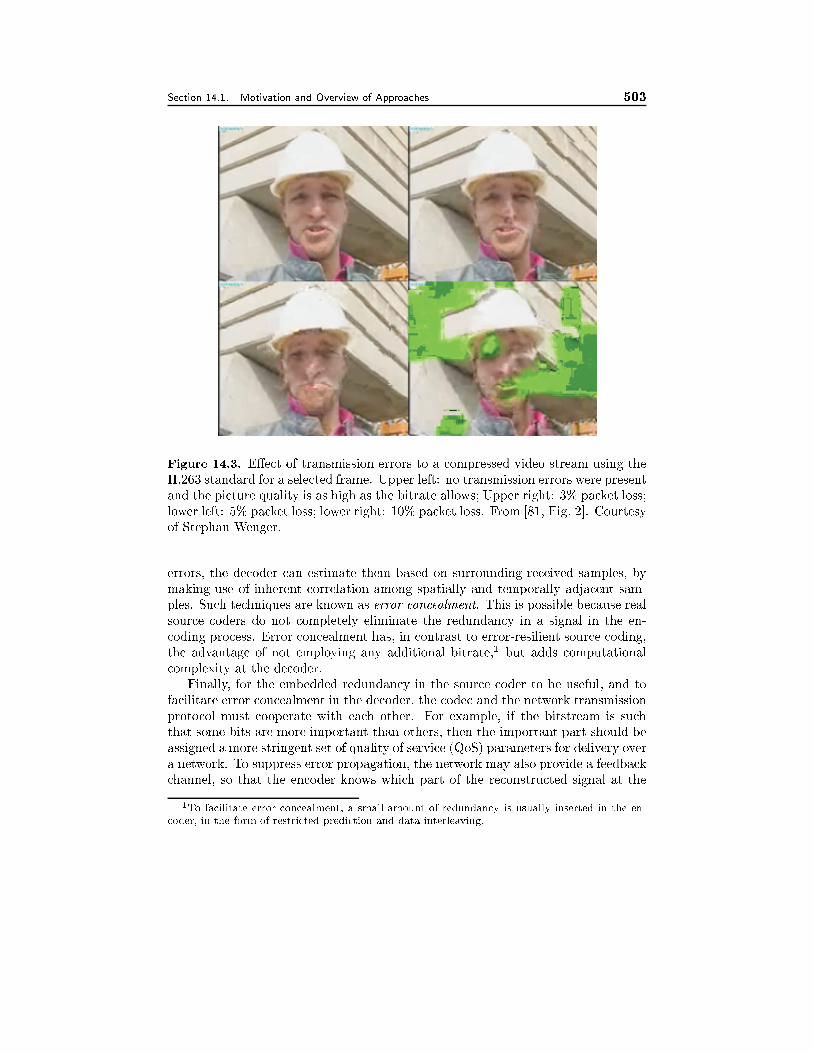
Section 14.1. Motivation and Overview of Approaches 503
Figure 14.3. E�ect of transmission errors to a compressed video stream using the
H.263 standard for a selected frame. Upper left: no transmission errors were present
and the picture quality is as high as the bitrate allows; Upper right: 3% packet loss;
lower left: 5% packet loss; lower right: 10% packet loss. From [81, Fig. 2]. Courtesy
of Stephan Wenger.
errors, the decoder can estimate them based on surrounding received samples, by
making use of inherent correlation among spatially and temporally adjacent sam-
ples. Such techniques are known as error concealment. This is possible because real
source coders do not completely eliminate the redundancy in a signal in the en-
coding process. Error concealment has, in contrast to error-resilient source coding,
the advantage of not employing any additional bitrate,1 but adds computational
complexity at the decoder.
Finally, for the embedded redundancy in the source coder to be useful, and to
facilitate error concealment in the decoder, the codec and the network transmission
protocol must cooperate with each other. For example, if the bitstream is such
that some bits are more important than others, then the important part should be
assigned a more stringent set of quality of service (QoS) parameters for delivery over
a network. To suppress error propagation, the network may also provide a feedback
channel, so that the encoder knows which part of the reconstructed signal at the
1To facilitate error concealment, a small amount of redundancy is usually inserted in the en-
coder, in the form of restricted prediction and data interleaving.
504 Error Control in Video Communications Chapter 14
decoder is damaged, and does not use this part for prediction of future samples.
To summarize, error control mechanisms devised for video transport can be cat-
egorized into four groups: i) those exercised at the transport level, including channel
coder, packetizer/multiplexer, and transport protocol; ii) those introduced at the
source encoder, to make the bit-stream more resilient to potential errors; iii) those
invoked at the decoder upon detection of errors, to conceal the e�ect of errors; and
�nally iv) those that require interactions between the source encoder and decoder,
so that the sender can adapt its operations based on the loss conditions detected
at the decoder. We will describe techniques in these four categories separately in
Secs. 14.3 to 14.6.
14.2 Typical Video Applications and Communication Networks
In this section, we describe di�erent types of video applications and characteristics
of practical networks. These are important factors to consider, because the neces-
sity for error control and the e�ectiveness of a technique depends on the type of
application as well as the underlying channel characteristics and network protocols.
14.2.1 Categorization of Video Applications
When considering error control in video transport, it is important to know whether
the underlying application requires real-time delivery, and what is the maximally
allowed average end-to-end delay (known as latency) and delay variation (known as
jitter). The name \real-time" means that the compressed data are transferred at
a speed that matches with the coded video source rate. For example, if the source
video is coded at 10 Mbps, then the throughput2 of the communication channel
devoted for this source should be at least 10 Mbps. Note that the source can be
generated in real-time (as in video conferencing applications) or o�-line (as in video
streaming applications). For all video applications except plain-old downloading,
real-time delivery is required. But some applications (e.g., streaming) can a�ord a
relatively large play-out delay. In this case, the receiver can use a large bu�er to
smooth out the jitter, so that the decoded video can be played out at a constant
frame rate, after an initial play-out delay. For such applications, a limited number
of retransmissions can be used to handle transmission errors. In the following, we
classify video applications based on their requirements in terms of real-time, latency,
and jitter.
Note that the end-to-end delay from a video source to a destination can be
contributed by several factors (See Fig. 14.4): encoder processing delay (including
acquiring the data and encoding), encoder bu�er delay (to smooth the rate variation
in the compressed bit stream), transmission delay (delay caused by the transmission
itself, which is usually very small, and that due to queuing and perhaps retransmis-
2\Throughput" means the e�ective end-to-end delivery rate. For example, a network may have
a raw bandwidth of 10 Mbps, but some data have to be retransmitted due to packet loss or timeout,
so that the actual throughput is lower than 10 Mbps.
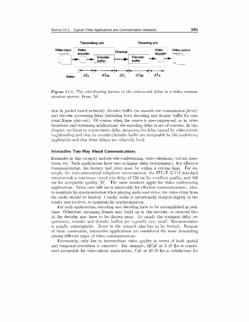
Section 14.2. Typical Video Applications and Communication Networks 505
Figure 14.4. The contributing factors to the end-to-end delay in a video commu-
nication system. From [58].
sion in packet-based network), decoder bu�er (to smooth out transmission jitter),
and decoder processing delay (including both decoding and display bu�er for con-
stant frame play-out). Of course, when the source is pre-compressed, as in video
broadcast and streaming applications, the encoding delay is not of concern. In this
chapter, we focus on transmission delay, assuming the delay caused by video encod-
ing/decoding and that by encoder/decoder bu�er are acceptable by the underlying
application and that these delays are relatively �xed.
Interactive Two-Way Visual Communications
Examples in this category include tele-conferencing, video telephony, virtual class-
room, etc. Such applications have very stringent delay requirements. For e�ective
communications, the latency and jitter must be within a certain limit. For ex-
ample, for inter-continental telephone conversations, the ITU-T G.114 standard
recommends a maximum round trip delay of 150 ms for excellent quality, and 400
ms for acceptable quality [37]. The same numbers apply for video conferencing
applications. Delay over 500 ms is intolerable for e�ective communications. Also,
to maintain lip synchronization when playing audio and video, the video delay from
the audio should be limited. Usually, audio is intentionally delayed slightly in the
sender and receiver, to maintain lip synchronization.
For such applications, encoding and decoding have to be accomplished in real-
time. Otherwise, incoming frames may build up at the encoder, or received bits
at the decoder may have to be thrown away. To satisfy the stringent delay re-
quirement, encoder and decoder bu�ers are typically very small. Retransmission
is usually unacceptable. Jitter in the network also has to be limited. Because
of these constraints, interactive applications are considered the most demanding
among di�erent types of video communications.
Fortunately, only low to intermediate video quality in terms of both spatial
and temporal resolution is expected. For example, QCIF at 5-10 fps is consid-
ered acceptable for video phone applications, CIF at 10-20 fps is satisfactory for
506 Error Control in Video Communications Chapter 14
most video conferencing scenarios. Furthermore, a moderate amount of compres-
sion/transmission artifacts is often tolerable.
One-Way Video Streaming
In this type of application, a live or pre-compressed video source is delivered to
one or multiple destinations. Instead of waiting for the entire video �le to arrive,
the receiving terminal starts to decode and play the video after an initial playout
delay, which can be up to a few seconds. Depending on the number of recipients, the
application can be further classi�ed as broadcast, multicast, and unicast. Television
broadcast is the most widely deployed video application. Video multicast, such as
the Mbone application, which allows any user on the Internet to view the video of
a live conference or seminar, is another important application. An application that
is becoming increasingly popular is streaming video from a pre-compressed video
database over the Internet, typically by a single user.
Obviously, the bandwidth requirements depend on the type of video material.
For digital TV broadcast over terrestrial, cable, or direct broadcast satellite (DBS)
channels, typically the video programs are in the BT.601 resolution, compressed
using the MPEG-2 format with bit rates between 3-10 Mbps. For HDTV, the bit
rates could be up to 20 Mbps. For multicasting and unicasting over the Internet or
wireless network, because of the limited bandwidth that can be devoted to each user
and the variability of the bandwidth and delay, lower quality video (CIF or lower,
compressed in MPEG-1 or MPEG4 or other proprietary formats) are typically used.
Because there is no interactive communication between the sender and receiver,
the latency could be fairly large, but the jitter must be limited, so that the received
stream can be decoded and played out smoothly at a constant frame rate, after
an initial delay. TV broadcast uses dedicated channels, which have guaranteed
bandwidth and very low jitter. For video multicast or unicast over the Internet,
where jitter could be large due to variability of the network conditions, a large
smoothing bu�er is typically installed in the receiver to absorb the jitter. The
larger the bu�er, the longer will be the playout delay, but the smoother will be the
displayed video.
In the case of multicast or unicast over the Internet, the potential recipients
may be connected to the network with di�erent access links (from 100 Mbps Fast-
Ethernet to a slow wireless modem link). Also, the receiving terminals may have
very di�erent computing powers (from a powerful workstation to a handheld battery
powered device). The video server must take these into account. For example, by
using scalable coding (Chap. 11), users with di�erent bandwidths and computing
powers may choose to extract di�erent portions of a compressed video stream. Video
streaming over the Internet and wireless IP networks are discussed in more detail
in Chap. 15.
The major di�erence between live and pre-compressed sources is, obviously, that
the live source has to be compressed in real-time, which signi�cantly increase the
complexity of the system at the transmission end. The encoding process and encoder
Section 14.2. Typical Video Applications and Communication Networks 507
bu�er will also contribute to additional delays.
One-Way Video Downloading
In this case, a pre-recorded video (and audio) is downloaded to a destination. The
receiving terminal does not start to play the material until the entire video has
arrived. This application is the least demanding in terms of delay requirement, al-
though excessive delay (because of the very low transmission bandwidth) may cause
the receiver to abort the downloading in the middle of a communication session.
Scalable coding and progressive transmission is desirable so that a low resolution
version of the video can be delivered relatively quickly. Because of the relaxed delay
requirement, retransmission can be used to handle any lost or erroneously delivered
part of the data. No special error control mechanisms are necessary, beyond those
typically used for data transfer.
14.2.2 Communication Networks
In this subsection, we describe di�erent types of networks and associated protocols
that may be used for video transport. For each network, we describe its character-
istics in terms of bandwidth, delay, delay variation (jitter) and loss rate (including
bit error and packet loss), as well as typical video applications carried over such
network.
Public Switched Telephone Network (PSTN)
The PSTN refers to the plain old telephone system (POTS). The best thing about
PSTN is that it is accessible by almost anyone in the US and, to a large extent, in the
world. However, the copper wire between the home and central oÆce has a limited
bandwidth. The fastest transmission rate by the most advanced modem technology
has now reached 56 Kbps. But this is still too low for carrying video with pleasing
quality. The ITU-T H.324 standard series (Sec. 13.3.2) has been developed for
multimedia communications over PSTN [36]. In H.324-based systems, the tradeo�
between bit error rate and bitrate of the modem link is adjusted via modem control
mechanisms. Most systems employ strong error control coding to achieve very low
error rates, at some expense of bitrate [81].
Even at 56 kbps (typically the achievable transmission rate for the payload on
a 56K modem is much lower), only a small window video (QCIF or lower) can be
provided. Although this may be adequate for visual communication purposes, it
is not nearly as pleasing as most people would like. Higher rates, up to 6 Mbps
in the downlink direction (from a central video server to home), are possible with
ADSL (Asymmetric Digital Subscriber Loop) modems [54]. ADSL is one of the
main transport media for streaming MPEG-1 and MPEG-2 movies through video-
on-demand services. A good discussion on issues involved in multimedia transport
over ADSL can be found in [96].
508 Error Control in Video Communications Chapter 14
Integrated Service Digital Network (ISDN)
ISDN is the �rst public network using digital transmission [66]. The data rate
can be multiples of basic channels (known as B channel) of 64 Kbps each, with the
multiplying factor p ranging from 1 to 24, corresponding to an aggregated bandwidth
from 64 to 1,536 Kbps. The basic subscription of ISDN, which is known as basic
rate interface, comes with 2B+D channels, where the D channel is 16 Kbps and is
used for return signaling. At 128 Kbps (p=2) for the signal delivery (64 Kbps in
each direction), only very low quality video (e.g., QCIF at 10 fps) can be achieved.
For a better video quality (i.e., CIF at 15 to 30 fps), at least 384 Kbps (p=6) is
required.
Like the phone line, communication over ISDN is based on circuit switching, i.e.,
an ISDN connection is dedicated to a particular conversation once the connection
is established. For this reason, the connection is very reliable. The �rst ITU-
T recommendation series for audiovisual conferencing, H.320, was developed for
ISDN [40]. H.320 is currently employed by the vast majority of video-conferencing
and video telephony equipment. The multiplex protocol H.221 [39] used by H.320
systems o�ers a bit oriented, practically error free video transmission channel with
a �xed video bitrate. Beyond the mandatory intra MB refresh mechanisms of the
video coding standard, no other error control tools are necessary [81].
Broadband ISDN (B-ISDN)
The above described ISDN service with the basic channel rate being 64 Kbps is more
accurately known as narrow-band ISDN or N-ISDN. This can be o�ered over existing
twisted pair local loop wiring. The term broad-band ISDN or B-ISDN [66] describes
ISDN services that o�er channels in excess of 64 Kbps, including H 0 channel with
a rate of 384 Kbps, H 11 channel with a rate of 1.536 Mbps, and H 12 channels with
a rate of 1.920 Mbps. This requires the use of higher bandwidth coaxial cables or
optical �bers. The bandwidth of B-ISDN is also speci�ed in multiples of 64 Kbps,
with the multiplying factor ranges from 1 to 65535.
For eÆcient usage of the bandwidth, the B-ISDN uses Asynchronous Transfer
Mode (ATM) packet switching technology with �xed size packets (known as cells).
No dedicated links are created for an established connection, which makes it less
reliable (i.e. with more delay variation and potential cell loss) than the circuit
switched ISDN. The very short cell size (53 Bytes with 48 bytes payload) makes it
suitable for real-time applications with low delay requirements. In such networks,
cell loss can occur due to traÆc congestion, although the loss ratio is quite low,
typically in the range of 10�6 to 10�4 for video services [3]. Generally, cell loss
can be considered as a sub-form of packet loss, whereby cells are extremely small
packets. The mechanisms to cope with cell losses, however, are di�erent, because it
is not e�ective to add synchronization markers at the beginning of each cell, from
a resilience/overhead tradeo� perspective.
The ATM network provides four types of services: constant bit rate (CBR),
variable bit rate (VBR), available bit rate (ABR) and unspeci�ed bit rate (UBR).
Section 14.2. Typical Video Applications and Communication Networks 509
Typically, video is carried in the VBR service, where the compressed bit stream has
to satisfy pre-set constraints in terms of average rate and peak rate. The allowance
of rate variation makes it possible to choose the video coding parameters to maintain
a relatively constant video quality, which is a desirable feature. Good reviews of
ATM networks and issues related to video transport over ATM can be found in
[3, 5].
Internet
The Internet is composed of multiple physical networks interconnected by comput-
ers known as routers. The most basic building block is known as a local area network
(LAN), which typically has bandwidth from 10 Mbps to 100 Mbps. Interconnected
LANs in a local region form a metropolitan area network (MAN), and �nally several
interconnected MANs form a wide area network (WAN). Communications on the
Internet is based on packet-switching. That is, the data to be delivered are truncated
into packets, with each packet given a header that speci�es the source and destina-
tion addresses. Each packet is delivered independently. Packets may be discarded
due to bu�er over ow at intermediate network nodes such as switches or routers or
considered as lost due to excessive long queuing delay. For real-time video applica-
tions, any packet arriving after the allowed delay time is also considered lost. The
transport of the packets is governed by the TCP/IP protocol suite, which includes
three important protocols: the Internet Protocol (IP), the User Datagram Protocol
(UDP) for unreliable connectionless packet delivery service, and the Transmission
Control Protocol (TCP) for reliable stream services. IP is the lower layer proto-
col on top of which UDP and TCP operate. TCP guarantees delivery by using
retransmission with acknowledgement [16].
The Internet and its associated TCP/IP protocol were originally designed for
data communications, which are not delay sensitive. For real-time services such as
video conferencing and video streaming, the retransmission mechanism in TCP is
not appropriate. To support such applications, Real-time Transport Protocol (RTP)
and its companion Real-Time Control Protocol (RTCP) have been developed. RTP
is built on top of UDP, but has added information in the header, including sequence
number and timing and synchronization information. RTP allows the detection of
lost packets based on sequence numbers as well as discarding of late packets at
the receiver end. RTCP is designed to provide QoS feedback (such as packet loss
rate) to the participants of a RTP session, so that the sender can adjust its op-
eration correspondingly (e.g., adjust the sending rate or change the error control
mechanism). A good discussion on the Internet protocols for supporting continu-
ous media services, including RTP/RTCP, real-time streaming protocol (RTSP) for
medium-on-demand, session initiation protocol (SIP) for internet telephony, session
announcement protocol (SAP) for broadcast applications, and session description
protocol (SDP) can be found in [62].
Typically, headers added at di�erent network layers will contribute to about 40
bytes in a packet. To gain a reasonable payload/overhead relationship, large data
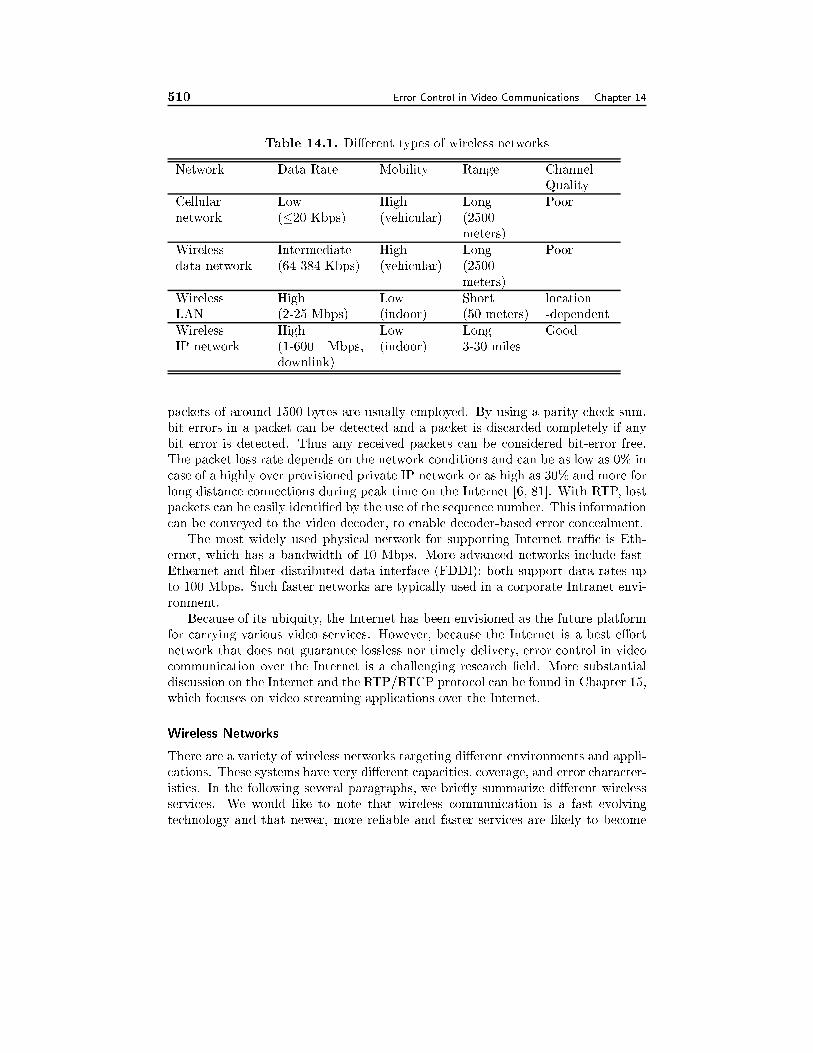
510 Error Control in Video Communications Chapter 14
Table 14.1. Di�erent types of wireless networks
Network Data Rate Mobility Range Channel
Quality
Cellular Low High Long Poor
network (�20 Kbps) (vehicular) (2500
meters)
Wireless Intermediate High Long Poor
data network (64-384 Kbps) (vehicular) (2500
meters)
Wireless High Low Short location
LAN (2-25 Mbps) (indoor) (50 meters) -dependent
Wireless High Low Long Good
IP network (1-600 Mbps,
downlink)
(indoor) 3-30 miles
packets of around 1500 bytes are usually employed. By using a parity check sum,
bit errors in a packet can be detected and a packet is discarded completely if any
bit error is detected. Thus any received packets can be considered bit-error free.
The packet loss rate depends on the network conditions and can be as low as 0% in
case of a highly over provisioned private IP network or as high as 30% and more for
long distance connections during peak time on the Internet [6, 81]. With RTP, lost
packets can be easily identi�ed by the use of the sequence number. This information
can be conveyed to the video decoder, to enable decoder-based error concealment.
The most widely used physical network for supporting Internet traÆc is Eth-
ernet, which has a bandwidth of 10 Mbps. More advanced networks include fast-
Ethernet and �ber distributed data interface (FDDI); both support data rates up
to 100 Mbps. Such faster networks are typically used in a corporate Intranet envi-
ronment.
Because of its ubiquity, the Internet has been envisioned as the future platform
for carrying various video services. However, because the Internet is a best e�ort
network that does not guarantee lossless nor timely delivery, error control in video
communication over the Internet is a challenging research �eld. More substantial
discussion on the Internet and the RTP/RTCP protocol can be found in Chapter 15,
which focuses on video streaming applications over the Internet.
Wireless Networks
There are a variety of wireless networks targeting di�erent environments and appli-
cations. These systems have very di�erent capacities, coverage, and error character-
istics. In the following several paragraphs, we brie y summarize di�erent wireless
services. We would like to note that wireless communication is a fast evolving
technology and that newer, more reliable and faster services are likely to become
Section 14.2. Typical Video Applications and Communication Networks 511
available by the time this book is published.
The cellular networks [27] are traditionally developed for mobile voice commu-
nication services but have now progressed to allow data transfer through wireless
modems. The data rate is limited to under 20 Kbps (the payload rate is much lower).
Alternatively, the cellular network can be connected to a packet-based wireless data
network, which enables one to transfer data between a mobile user and a wired
terminal over the Internet (such as in web browsing applications). For example, the
basic GPRS (general packet radio service) wireless access network o�ers a payload
bit rate ranging from 9 to 21.4 Kbps using single time slot, while the enhanced
GRPS wireless access technology (known as EDGE) can provide bit rates ranging
from 8.8 to around 59.2 Kbps [9]. By using multiple time slots, the raw data rate can
be as high as 170 Kbps. The available data rate is location-dependent, with higher
rates when the user is closer to the base station. The upcoming third generation
(3G) wireless systems promise to provide higher data rates and ubiquitous coverage
by using higher carrier frequencies, wider bandwidth and more sophisticated tech-
niques for multiple access, error control, and signal detection. The outdoor data
rates range from 144 Kbps to 384 Kbps depending on the mobile speed and distances
between terminals, and the indoor data rates will be at least 2 Mbps. The BER for
data transmission will be below 10�6. Real-time audiovisual communication will be
an integral part of the 3G services. In general, any wireless channel is quite noisy,
with high bit error rates. But the use of rate adaptation, FEC and ARQ yields an
almost error-free environment for data transmission. For video transmission, where
ARQ has to be limited, one has to cope with quite high bit error rates and packet
loss rates. This is discussed further when we consider wireless video transmission
using the H.223 multiplex protocol.
A wireless LAN refers to a set of information devices (typically indoor, station-
ary or slowly moving) connected into a LAN using wireless connections. Either
IP or ATM transport protocols can be used, which are referred as mobile IP and
wireless ATM, respectively. The main challenge in adapting conventional IP and
ATM protocols to wireless environments is how to provide continuous network con-
nectivity to mobile nodes and how to handle hand-o�s, when the mobile terminal
is switching from the coverage area of one access point to another. Achievable bit
rates depend on the carrier frequencies. For example, LANs conforming to the IEEE
802.11 standard can have bit rates up to 11 Mbps (with lower payload rate). The
connection in a wireless LAN is either very good (e.g. BER lower than 10�5), when
the user is close to the access point, or very bad (e.g. BER higher than 10�2), when
the user is far from the access point. The packet loss rates depend on the packet
size and error detection and correction methods incorporated within the packet.
Broadband Wireless IP networks refer to the access to the Internet by home or
business users through small roof-top antennas communicating to a base station
using microwave radio. This includes multichannel multipoint distribution service
(MMDS) and local multipoint distribution service (LMDS). LMDS uses higher car-
rier frequencies than MMDS, and thus enables a higher data rate (typically up to
100 Mbps, but can be as high as 600 Mbps) than MMDS (up to 1 Mbps). However,
512 Error Control in Video Communications Chapter 14
LMDS is e�ective within a much shorter range between the base-station and the
client site (3 miles vs. 30 miles).
Table 14.1 summarizes the characteristics of the networks discussed above. A
good review of various wireless networks can be found in [9].
DiÆculties for video transport over wireless networks lie in the low bandwidth,
high error rate (random bit error as well as long bursts because of the multipath
fading e�ect), and most importantly, the uctuation of available bandwidth and
error characteristics. Such variability is particularly acute when mobile stations
are involved. A wireless video communication system therefore must be adaptive
both in rate and error resilience. To meet such requirements, most proposals for
wireless video transport use layered coding with unequal error protection. It is
worth noting that, for real-world applications, quite sophisticated FEC codes are
used to reduce the bit error rates signi�cantly. On top of FEC, real-world systems
generally employ certain forms of channel multiplexers that often include transport
protocol functionality as well, thereby reducing the error rates further.
Most wireless interactive multimedia communication systems employ H.223 [38]
and its \mobile extensions" as the transport/multiplex protocol on top of the bit-
oriented channel [81]. The mobile extensions form a hierarchy with �ve di�erent
levels, which allows for a scalable tradeo� between the robustness against bit er-
rors of the multiplexer itself and the overhead incurred by that multiplexer. Most
research for video coding on top of the H.223 transport is performed with average
burst lengths in the neighborhood of 16 bits, and BERs between 10�5 and 10�3.
H.223 conveys media data including compressed video in the form of packets of
variable size. Typical packet sizes are around 100 bytes to ensure good delay char-
acteristics. If bit errors damage the protocol structures of H.223 beyond the repair
facilities of the employed level (a condition known as multiplex errors), then whole
packets can get lost as well. Therefore, video transmission on top of H.223 has to
cope with packet losses.
For a good discussion on the issues involved in video transport over wireless
systems, see [76, 25]. Video streaming over wireless IP networks is further considered
in Chap. 15.
Broadcast Channels: Terrestrial, Cable, Satellite
This transport environment is used for broadcasting of digital TV including HDTV
programs using the MPEG-2 video coding and transport streams. The compressed
data are carried over �xed size transport packets of 188 bytes each. Regardless
of the underlying wireline or wireless physical layer, the channel coders and the
MPEG-2 transport layer ensure an almost error free environment. For SDTV, the
available bandwidth is divided into program channels that can carry between 3-10
Mbps each. For HDTV, 20 Mbps is typically allocated. A good reference on digital
TV services using direct broadcast satellite (DBS) is [55].
Table 14.2 summarizes the characteristics of major video communications appli-
cations, including the standards used, the target network, and transmission char-
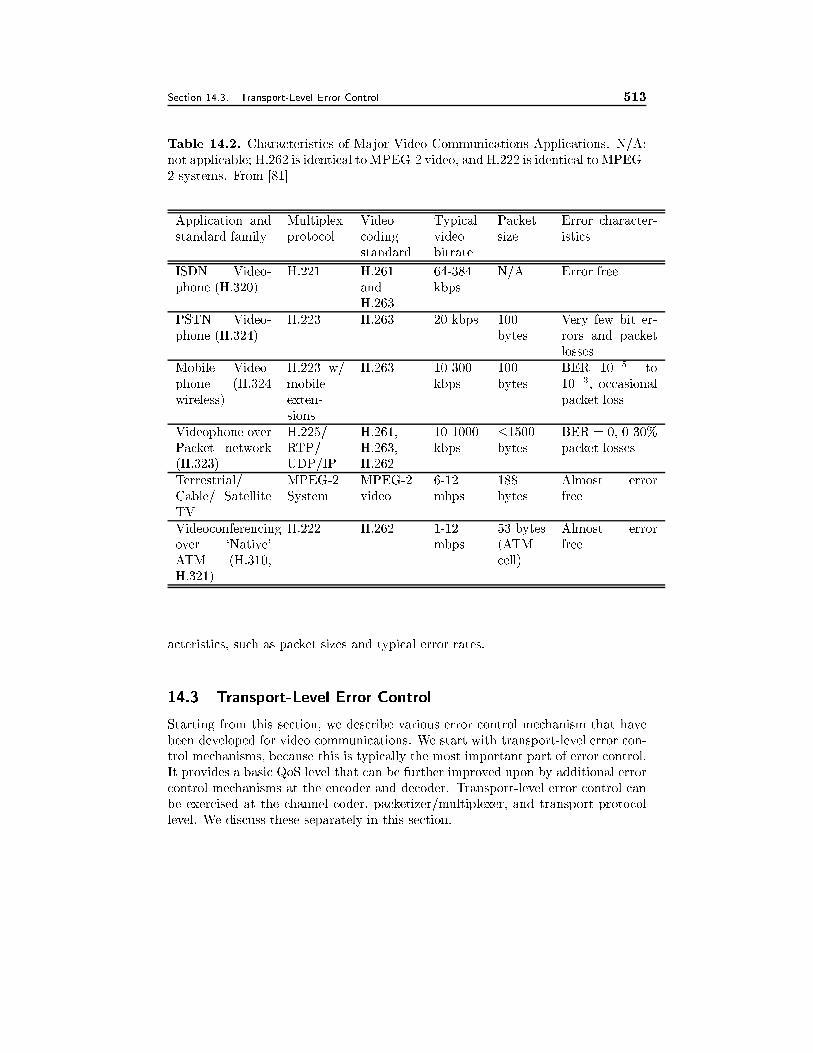
Section 14.3. Transport-Level Error Control 513
Table 14.2. Characteristics of Major Video Communications Applications. N/A:
not applicable; H.262 is identical to MPEG-2 video, and H.222 is identical to MPEG-
2 systems. From [81]
Application and
standard family
Multiplex
protocol
Video
coding
standard
Typical
video
bitrate
Packet
size
Error character-
istics
ISDN Video-
phone (H.320)
H.221 H.261
and
H.263
64-384
kbps
N/A Error free
PSTN Video-
phone (H.324)
H.223 H.263 20 kbps 100
bytes
Very few bit er-
rors and packet
losses
Mobile Video-
phone (H.324
wireless)
H.223 w/
mobile
exten-
sions
H.263 10-300
kbps
100
bytes
BER=10�5 to
10�3, occasional
packet loss
Videophone over
Packet network
(H.323)
H.225/
RTP/
UDP/IP
H.261,
H.263,
H.262
10-1000
kbps
�1500
bytes
BER = 0, 0-30%
packet losses
Terrestrial/
Cable/ Satellite
TV
MPEG-2
System
MPEG-2
video
6-12
mbps
188
bytes
Almost error
free
Videoconferencing
over `Native'
ATM (H.310,
H.321)
H.222 H.262 1-12
mbps
53 bytes
(ATM
cell)
Almost error
free
acteristics, such as packet sizes and typical error rates.
14.3 Transport-Level Error Control
Starting from this section, we describe various error control mechanism that have
been developed for video communications. We start with transport-level error con-
trol mechanisms, because this is typically the most important part of error control.
It provides a basic QoS level that can be further improved upon by additional error
control mechanisms at the encoder and decoder. Transport-level error control can
be exercised at the channel coder, packetizer/multiplexer, and transport protocol
level. We discuss these separately in this section.
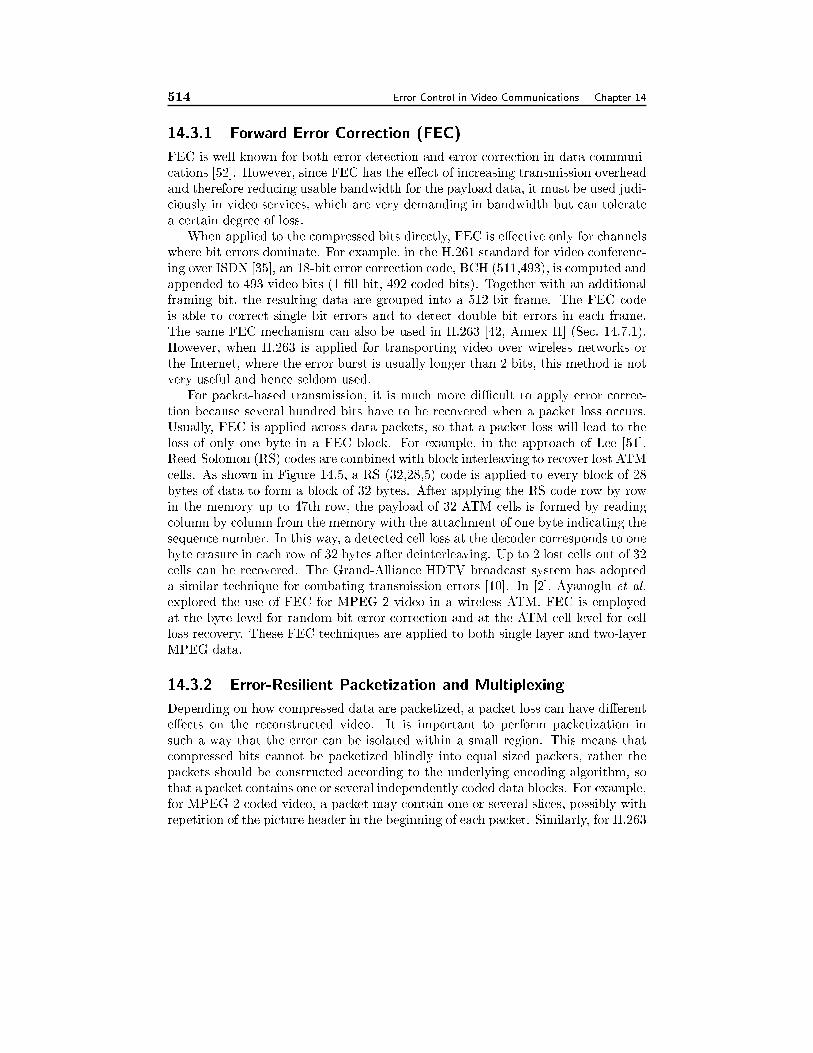
514 Error Control in Video Communications Chapter 14
14.3.1 Forward Error Correction (FEC)
FEC is well known for both error detection and error correction in data communi-
cations [52]. However, since FEC has the e�ect of increasing transmission overhead
and therefore reducing usable bandwidth for the payload data, it must be used judi-
ciously in video services, which are very demanding in bandwidth but can tolerate
a certain degree of loss.
When applied to the compressed bits directly, FEC is e�ective only for channels
where bit errors dominate. For example, in the H.261 standard for video conferenc-
ing over ISDN [35], an 18-bit error correction code, BCH (511,493), is computed and
appended to 493 video bits (1 �ll bit, 492 coded bits). Together with an additional
framing bit, the resulting data are grouped into a 512-bit frame. The FEC code
is able to correct single bit errors and to detect double bit errors in each frame.
The same FEC mechanism can also be used in H.263 [42, Annex H] (Sec. 14.7.1).
However, when H.263 is applied for transporting video over wireless networks or
the Internet, where the error burst is usually longer than 2 bits, this method is not
very useful and hence seldom used.
For packet-based transmission, it is much more diÆcult to apply error correc-
tion because several hundred bits have to be recovered when a packet loss occurs.
Usually, FEC is applied across data packets, so that a packet loss will lead to the
loss of only one byte in a FEC block. For example, in the approach of Lee [51],
Reed-Solomon (RS) codes are combined with block interleaving to recover lost ATM
cells. As shown in Figure 14.5, a RS (32,28,5) code is applied to every block of 28
bytes of data to form a block of 32 bytes. After applying the RS code row by row
in the memory up to 47th row, the payload of 32 ATM cells is formed by reading
column by column from the memory with the attachment of one byte indicating the
sequence number. In this way, a detected cell loss at the decoder corresponds to one
byte erasure in each row of 32 bytes after deinterleaving. Up to 2 lost cells out of 32
cells can be recovered. The Grand-Alliance HDTV broadcast system has adopted
a similar technique for combating transmission errors [10]. In [2], Ayanoglu et al.
explored the use of FEC for MPEG-2 video in a wireless ATM. FEC is employed
at the byte level for random bit error correction and at the ATM cell level for cell
loss recovery. These FEC techniques are applied to both single layer and two-layer
MPEG data.
14.3.2 Error-Resilient Packetization and Multiplexing
Depending on how compressed data are packetized, a packet loss can have di�erent
e�ects on the reconstructed video. It is important to perform packetization in
such a way that the error can be isolated within a small region. This means that
compressed bits cannot be packetized blindly into equal sized packets, rather the
packets should be constructed according to the underlying encoding algorithm, so
that a packet contains one or several independently coded data blocks. For example,
for MPEG-2 coded video, a packet may contain one or several slices, possibly with
repetition of the picture header in the beginning of each packet. Similarly, for H.263
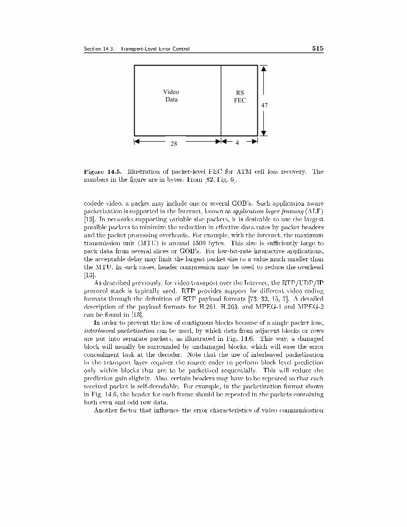
Section 14.3. Transport-Level Error Control 515
4
47
Video
DataRS
FEC
28
Figure 14.5. Illustration of packet-level FEC for ATM cell loss recovery. The
numbers in the �gure are in bytes. From [82, Fig. 6].
codede video, a packet may include one or several GOB's. Such application aware
packetization is supported in the Internet, known as application layer framing (ALF)
[13]. In networks supporting variable size packets, it is desirable to use the largest
possible packets to minimize the reduction in e�ective data rates by packet headers
and the packet processing overheads. For example, with the Internet, the maximum
transmission unit (MTU) is around 1500 bytes. This size is suÆciently large to
pack data from several slices or GOB's. For low-bit-rate interactive applications,
the acceptable delay may limit the largest packet size to a value much smaller than
the MTU. In such cases, header compression may be used to reduce the overhead
[13].
As described previously, for video transport over the Internet, the RTP/UDP/IP
protocol stack is typically used. RTP provides support for di�erent video coding
formats through the de�nition of RTP payload formats [73, 32, 15, 7]. A detailed
description of the payload formats for H.261, H.263, and MPEG-1 and MPEG-2
can be found in [13].
In order to prevent the loss of contiguous blocks because of a single packet loss,
interleaved packetization can be used, by which data from adjacent blocks or rows
are put into separate packets, as illustrated in Fig. 14.6. This way, a damaged
block will usually be surrounded by undamaged blocks, which will ease the error
concealment task at the decoder. Note that the use of interleaved packetization
in the transport layer requires the source coder to perform block level prediction
only within blocks that are to be packetized sequentially. This will reduce the
prediction gain slightly. Also, certain headers may have to be repeated so that each
received packet is self-decodable. For example, in the packetization format shown
in Fig. 14.6, the header for each frame should be repeated in the packets containing
both even and odd row data.
Another factor that in uence the error characteristics of video communication
516 Error Control in Video Communications Chapter 14
Frame 1
Even Row
Data
Frame 2
Odd Row
Data
Frame 1
Odd Row
Data
Frame 2
Even Row
Data
......
Packet 1 Packet 2 Packet 3 Packet 4 ......
Figure 14.6. An example of interleaved packetization.
is how are the video and other data (audio, control) multiplexed and how is the
header protected. An error in the multiplex header can cause the video data be mis-
delivered, causing large chunks of data to disappear at the receiver [76]. To prevent
such events from happening, typically, each packet is led by a long synchronization
ag, and the header is heavily protected using FEC. A good example is the multi-
plexing standard H.223 [38], developed under the umbrella of the H.324 system for
low-bit rate multimedia communications. It is designed to support multiplexing of
data from multiple sources on a circuit-switched network (e.g., wireline and wireless
modems). H.223 o�ers a hierarchical, multilevel multiplexing structure, allowing for
a scalable tradeo� between the robustness against bit errors of the multiplexer itself
and the overhead incurred by that multiplexer. Level 0, which is targeted for wire-
line environments, use a short sync ag and no FEC on the header. Higher levels,
which are targeted for more error prone environments such as a mobile wireless
modem, use increasingly longer sync ags and stronger protection for the header.
14.3.3 Delay-Constrained Retransmission
Beyond the low level error control mechanism such as FEC, error resilient packetiza-
tion and multiplexing, the upper layer transport protocol can exercise error control,
typically in the form of automatic retransmission request (ARQ), which requests re-
transmission upon the detection of lost or overly delayed packets, as is done in TCP.
Retransmission has been used very successfully for non real-time data transmission,
but it has been generally considered as unacceptable for real-time video applications
because of the delay incurred. This is in fact not always the case. For example,
for a coast-to-coast interactive service, one retransmission adds only about 70 ms
delay, which can be acceptable [59]. For one-way real-time video applications such
as Internet video streaming and broadcast, the delay allowance can be further re-
laxed to a few seconds so that several retransmissions are possible. Retransmission
has also been considered inappropriate for multipoint video conferencing because
the retransmission requests from a large number of decoders can overwhelm the
encoder. However, when a multipoint control unit (MCU) is used in a multipoint
conference, the paths between the encoder and the MCU, and between the MCU
and the decoders are simply point-to-point. Retransmission can be applied in these
paths separately. Another concern about using retransmission is that retransmis-
Section 14.3. Transport-Level Error Control 517
sion may worsen the problem, because it will add more traÆc on the network and
thus further increase the packet loss rate. However, if retransmission is controlled
appropriately, the end-to-end quality can be improved. For example, the encoder
can reduce its current output rate so that the sum of the encoder output and the
retransmitted data is kept below a given total data rate.
Obviously, for real-time applications, retransmission must be constrained so that
the incurred delay is within the acceptable range. Instead of trying retransmission
inde�nitely to recover a lost packet, as done in TCP, the number of retransmission
trials can be determined by the desired delay [53]. One can also combine layered
coding (Sec. 14.4.4) with prioritized retransmission, by placing the base layer pack-
ets of a layered coder in the front of the transmission queue to increase the number
of retransmission trials for the base layer [64]. Finally, one can send multiple copies
of a lost packet in each single retransmission trial, hoping at least one get through
in time [98]. The number of retransmission trials and the number of retransmission
copies for a lost packet can be determined according to its importance. For exam-
ple, a base layer packet can be retransmitted several times, each time with multiple
copies, while an enhancement layer packet can be simply dropped. Another con-
strained retransmission scheme speci�cally designed for video streaming application
is described in Chap. 15.
14.3.4 Unequal Error Protection
The binary bits in a compressed video bitstream are not equally important. For
example, the picture header and other side information are much more important
than the block data, in block-based hybrid coder. These important bits should be
protected so that they can be delivered with a much lower error rate. When layered
coding is used at the source coder (Sec. 14.4.4), the transport controller must assign
appropriate priority to di�erent layers, which is a form of transport level control.
Di�erent networks may implement transport prioritization using di�erent means.
In ATM networks, there is one bit in the ATM cell header that signals its prior-
ity. When traÆc congestion occurs, a network node can choose to discard the cells
having low priority �rst. Transport prioritization can also be implemented by us-
ing di�erent levels of power to transmit the substreams in a wireless network. In
the Internet, the latest RTP speci�cation de�nes generic mechanisms for transport-
ing layered video bitstreams [63]. There are also network support for prioritized
delivery through di�erentiated services [4]. In either wireless networks or the Inter-
net, prioritization can be realized with di�erent error control treatments to various
layers. For example, retransmission and strong FEC can be applied for the base
layer while no retransmission and weaker FEC may be applied to the enhancement
layers. In the extreme case, the most important information can be duplicated.
For example, dual transmission for picture header information and quantization
matrix has been proposed for MPEG video [70]. Another way to provide di�erent
levels of protection is by using di�erent transport protocols. For example, in the
video-on-demand system described in [14], TCP is used for transmission of a very
518 Error Control in Video Communications Chapter 14
small amount of high-priority data (session control data) before a service session
and UDP is employed for the remaining low-priority data (video data) during the
session.
14.4 Error-Resilient Encoding
The previous section described various error control mechanisms that can be ex-
ercised at the transport level. These methods are applied to coded video streams,
attempting to detect, correct, and if necessary and feasible, retransmit damaged
data. Such methods, even when applicable, may not completely correct the error,
so that the received bitstream at the decoder still contain errors (bit error as well
as packet loss). In this section, we describe source coding methods that can pro-
duce a bit stream that is robust to transmission errors, so that an error will not
adversely a�ect the decoder operation and lead to unacceptable distortions in the
reconstructed video quality.
Compared to source coders that are optimized for coding eÆciency, such coders
typically are less eÆcient in that they use more bits to obtain the same video quality
in the absence of any transmission errors. These extra bits are called redundancy
bits,3 and they are introduced to enhance the video quality when the bitstream
is corrupted by transmission errors. The design goal in error-resilient coding is to
achieve the best decoded video quality for a given amount of redundancy, or minimize
the incurred redundancy while maintaining a prescribed quality level, both under an
assumed channel environment. There are many ways to introduce redundancy in
the bitstream. Some of the techniques help to isolate the error (Sec. 14.4.1), while
others enable the decoder to perform better error concealment upon detection of
errors (Secs. 14.4.2 and 14.4.3). Yet another group of techniques are aimed at
guaranteeing a basic level of quality and providing a graceful degradation upon the
occurrence of transmission errors (Secs. 14.4.4 and 14.4.5).
14.4.1 Error Isolation
One main cause for the sensitivity of a compressed video stream to transmission
errors is that a video coder uses VLC to represent various symbols. Any bit errors or
lost bits in the middle of a codeword can not only make this codeword undecodable
but also make the following codewords undecodable or decoded to wrong symbols,
even if they are received correctly. Error isolation techniques, as the name implies,
try to isolate the e�ect of a transmission error within a limited region. This is often
achieved by placing \resynchronization markers" in the compressed bitstream, and
by a technique known as \data partitioning". Both have been incorporated into
MPEG-4 and H.263 standards.
3Such bits are also referred to as \overhead".
Section 14.4. Error-Resilient Encoding 519
Inserting Resynchronization Markers
One simple and e�ective approach for enhancing encoder error- resilience is by in-
serting resynchronization markers periodically. These markers are designed such
that they can be easily distinguished from all other codewords and small pertur-
bation of these codewords. Usually some header information (regarding the spatial
and temporal locations or other information that is needed to decode subsequent
bits) is attached immediately after the resynchronization information. This way,
the decoder can resume proper decoding upon the detection of a resynchronization
marker. Obviously, insertion of resynchronization markers will reduce the coding
eÆciency. First, the longer and more frequent are such markers, the more bits will
be used for them. Second, the use of synchronization markers typically interrupts
in-picture prediction mechanisms, such as MV or DC coeÆcient prediction, which
adds even more bits. But longer and frequently inserted markers would also enable
the decoder to regain synchronization more quickly, so that a transmission error
a�ects a smaller region in the reconstructed frame. Hence in practical video coding
systems, relatively long synchronization codewords are used.
Data Partitioning
In the absence of any other error resilience tools, the data between the error loca-
tion and the �rst following resynchronization marker would have to be discarded.
To achieve better error isolation, data between two synchronization points can be
further partitioned into �ner logic units, with secondary markers in between. This
way, logic units before an error location can still be decoded. Such markers can be
shorter than the primary markers, because they only need to be free from emulation
by data in the logic units that immediately proceed them. This approach is used in
the error-resilience modes of MPEG-4 and H.263 standards, by which MB headers,
motion vectors and DCT coeÆcients of all MBs in a slice or GOB are put into
separate logic units. This way, if an error happens, say in the logic unit containing
DCT coeÆcients, the header and motion information of the MBs contained in the
previous logic units are still decodable.
14.4.2 Robust Entropy Coding
In addition to error isolation by inserting synchronization codewords or partitioning
the data into independent segments, one can also directly modify entropy coding
methods so that the resulting bitstream is more robust to transmission errors. We
present two such techniques below.
Reversible Variable Length Coding (RVLC)
In the above discussion, we have assumed that once an error occurs, the decoder
discards all the bits until a resynchronization codeword is identi�ed. With RVLC
[72], the decoder can not only decode bits after a resynchronization codeword, but
also decode the bits before the next resynchronization codeword, from the backward
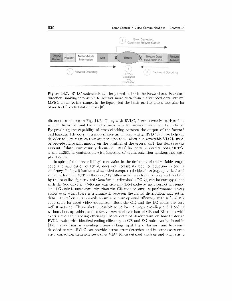
520 Error Control in Video Communications Chapter 14
Figure 14.7. RVLC codewords can be parsed in both the forward and backward
direction, making it possible to recover more data from a corrupted data stream.
MPEG-4 syntax is assumed in the �gure, but the basic priciple holds true also for
other RVLC-coded data. From [8].
direction, as shown in Fig. 14.7. Thus, with RVLC, fewer correctly received bits
will be discarded, and the a�ected area by a transmission error will be reduced.
By providing the capability of cross-checking between the output of the forward
and backward decoder, at a modest increase in complexity, RVLC can also help the
decoder to detect errors that are not detectable when non-reversible VLC is used,
or provide more information on the position of the errors, and thus decrease the
amount of data unnecessarily discarded. RVLC has been adopted in both MPEG-
4 and H.263, in conjunction with insertion of synchronization markers and data
partitioning.
In spite of the \reversibility" constraint in the designing of the variable length
code, the application of RVLC does not necessarily lead to reduction in coding
eÆciency. In fact, it has been shown that compressed video data (e.g. quantized and
run-length coded DCT coeÆcients, MV di�erences), which can be very well modeled
by the so-called \generalized Gaussian distribution" (GGD), can be entropy coded
with the Golomb-Rice (GR) and exp-Golomb (EG) codes at near perfect eÆciency.
The EG code is more attractive than the GR code because its performance is very
stable even when there is a mismatch between the model distribution and actual
data. Therefore it is possible to achieve near optimal eÆciency with a �xed EG
code table for most video sequences. Both the GR and the EG codes are very
well structured. This makes it possible to perform entropy encoding and decoding
without look-up-tables, and to design reversible versions of GR and EG codes with
exactly the same coding eÆciency. More detailed descriptions on how to design
RVLC tables with identical coding eÆciency as GR and EG codes can be found in
[86]. In addition to providing cross-checking capability of forward and backward
decoded results, RVLC can provide better error detection and in some cases even
error correction than non-reversible VLC. More detailed analysis and comparison
Section 14.4. Error-Resilient Encoding 521
of the decoder operation for reversible and non-reversible VLC can be found in [85].
Error-Resilient Entropy Coding (EREC)
Instead of using synchronization codewords to enable the decoder to resume decod-
ing, the EREC method employs a way of reordering coded bits so that the decoder
can regain synchronization at the start of each block [60]. Speci�cally, variable
length bit streams from individual blocks are distributed into slots of equal sizes.
Initially, the coded data for each image block are placed into the designated slot
for the block either fully or partially. Then, a prede�ned o�set sequence is used to
search for empty slots to place any remaining bits of blocks that are bigger than
the slot size. This is done until all the bits are packed into one of the slots. Because
the size of each slot is �xed, the decoder can regain synchronization at the start of
each block. It also ensures that the beginning of each block is more immune to error
propagation than those at the end. Because EREC does not insert any bits just for
synchronization purpose, the redundancy introduced is negligible. Application of
EREC in MPEG-2 and H.263 coders have been considered in [71, 48].
14.4.3 Error-Resilient Prediction
As we have seen, the use of VLC makes a compressed bitstream very sensitive to
transmission errors. Another major cause for the sensitivity is the use of temporal
prediction. Once an error occurs so that a reconstructed frame at the decoder
di�ers from that assumed at the encoder, the reference frames used in the decoder
from there onwards will di�er from those used at the encoder, and consequently all
subsequent reconstructed frames will be erroneous. This error propagation e�ect
has been shown previously in Fig. 14.2. The use of spatial prediction for the DC
coeÆcients and MVs will also cause error propagation, although it is con�ned within
the same frame. Error-resilient prediction refer to techniques that constrain the
prediction loop so as to con�ne error propagation within a short time interval.
Insertion of Intra-Blocks or Frames
One way to stop temporal error propagation is by periodically inserting intra-coded
pictures or MBs. Using an I-frame can cause a surge in the output bit rate, and
thus is typically not acceptable for interactive applications due to delay constraints.
For such applications, using a suÆciently high number of intra-coded MBs is an
eÆcient and highly scalable tool for error resilience.
When employing intra MBs for error resilience purposes, both the number of
such MBs and their spatial placement have to be determined. The number of nec-
essary intra MBs is dependent on the quality of the channel and the error control
mechanism applied at the transport level. Many practical systems provide infor-
mation about the network quality, or heuristic means to gain such information.
Examples include antenna signal strength in wireless environments, or RTCP re-
ceiver reports on Internet connections. The study in [67] analyzed the dependence
522 Error Control in Video Communications Chapter 14
of the overall distortion at the decoder on the intra-MB rate at the encoder, the
channel coding rate (assuming Reed-Solumn coding), the channel error parameters
(random loss rate and burst length). Based on this relation, one can �nd the optimal
intra-MB rate and/or channel coding rate, for given channel error characteristics.
For the spatial placement of intra MBs, the approaches proposed can be cat-
egorized as either heuristic or rate-distortion (RD) optimized. Heuristic methods
include random placement, placement in the area of high activity. Hybrid schemes
that additionally consider the time of the last intra update of a given MB were also
considered. These methods are simple and in general perform well. The RD opti-
mization approach can further improve the performance at the expense of increased
encoder complexity.
Recall that in the absence of transmission errors, the coding mode for each
MB can be determined based on the RD trade-o� obtained by di�erent modes
(Sec. 9.3.3). Ideally, the mode that leads to the maximum reduction in the distortion
per bit spent should be used. For error resilience purpose, the same RD optimization
approach can be taken, but the encoder must take into account of the fact that
the current MB and previous MB's may be lost, when calculating the distortion
associated with each coding mode. Several approaches have been developed based
on this framework, and they di�er in the way the expected distortion in the decoder
is calculated, and the way the channel error is modeled [17, 94, 89].
For example, the algorithm in [17] takes as input a mid-term prediction of the
packet loss rate, p. EachMB is coded in the intra, inter, and skip modes respectively,
and for each mode, the resulting rate R(modei) and distortion D1(modei) assuming
lossless transmission of the MB are measured. Then, for the same set of coding
modes, another set of distortions, D2(modei), is calculated under the assumption
that the coded MB got lost during transmission. The error propagation e�ect in
an inter-coded MB as well as error concealment in the decoder for a lost MB are
taken into account in the above distortion measurement. For each coding mode,
the expected distortion D(modei) = (1�p)D1(modei)+pD2(modei) is determined.
The coding mode that leads to the best rate-distortion trade-o� is determined. This
is accomplished by determining the LagrangianD(modei)+�R(modei) for di�erent
modes, for a �xed �; and �nding the mode that has the minimal Lagrangian. The
Lagrangian multiplier � is chosen based on the target bit rate.
Finally, when a feedback channel is available, it can be used to convey infor-
mation about missing or damaged MB data to trigger intra coding at the sender.
These schemes are discussed in Sec. 14.6.
Independent Segment Prediction
Another approach to limit the extent of error propagation is to split the data domain
into several segments, and perform temporal/spatial prediction only within the same
segment. This way, the error in one segment will not a�ect another segment. For
example, a frame can be divided into multiple regions (e.g., a region can be a GOB
or slice), and region one can only be predicted from region one in the previous
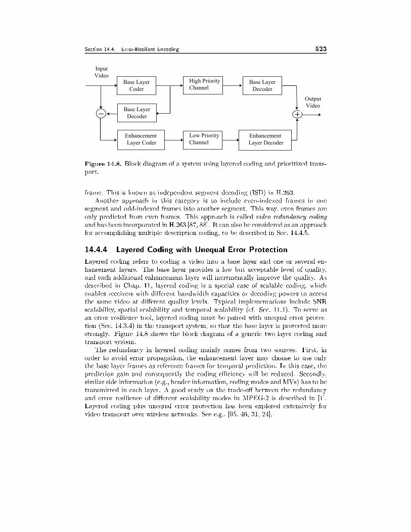
Section 14.4. Error-Resilient Encoding 523
Base Layer
Coder
Base Layer
Decoder
Enhancement
Layer Coder
High Priority
Channel
Low Priority
Channel
Base Layer
Decoder
Enhancement
Layer Decoder
Input
Video
Output
Video
Figure 14.8. Block diagram of a system using layered coding and prioritized trans-
port.
frame. This is known as independent segment decoding (ISD) in H.263.
Another approach in this category is to include even-indexed frames in one
segment and odd-indexed frames into another segment. This way, even frames are
only predicted from even frames. This approach is called video redundancy coding
and has been incorporated in H.263 [87, 88]. It can also be considered as an approach
for accomplishing multiple description coding, to be described in Sec. 14.4.5.
14.4.4 Layered Coding with Unequal Error Protection
Layered coding refers to coding a video into a base layer and one or several en-
hancement layers. The base layer provides a low but acceptable level of quality,
and each additional enhancement layer will incrementally improve the quality. As
described in Chap. 11, layered coding is a special case of scalable coding, which
enables receivers with di�erent bandwidth capacities or decoding powers to access
the same video at di�erent quality levels. Typical implementations include SNR
scalability, spatial scalability and temporal scalability (cf. Sec. 11.1). To serve as
an error resilience tool, layered coding must be paired with unequal error protec-
tion (Sec. 14.3.4) in the transport system, so that the base layer is protected more
strongly. Figure 14.8 shows the block diagram of a generic two-layer coding and
transport system.
The redundancy in layered coding mainly comes from two sources. First, in
order to avoid error propagation, the enhancement layer may choose to use only
the base layer frames as reference frames for temporal prediction. In this case, the
prediction gain and consequently the coding eÆciency will be reduced. Secondly,
similar side information (e.g., header information, coding modes and MVs) has to be
transmitted in each layer. A good study on the trade-o� between the redundancy
and error resilience of di�erent scalability modes in MPEG-2 is described in [1].
Layered coding plus unequal error protection has been explored extensively for
video transport over wireless networks. See e.g., [95, 46, 31, 24].

524 Error Control in Video Communications Chapter 14
MDC
Encoder
Channel 1Decoder
0
Decoder
1
Decoder
2
Channel 2
Source
Signal
Decoded
Signal
from S1
Decoded
Signal
from
S1 and S2
Decoded
Signal
from S2
S1
S2
MDC Decoder
Figure 14.9. Illustration of multiple description coding and decoding.
14.4.5 Multiple Description Coding
Layered coding described in the previous subsection can o�er error resilience when
the base layer is transmitted in an essentially error-free channel, realized via strong
FEC and retransmission. However, in certain applications, it may not be feasible
or cost e�ective to guarantee lossless transmission of any data. In this case, a loss
in the base layer can lead to a disastrous e�ect in the decoded visual quality. An
alternative approach to combat transmission errors is by using multiple descrip-
tion coding (MDC). With this coding scheme, several bit streams (referred to as
descriptions) of the same source signal are generated and transmitted over sepa-
rate channels. Each channel may be temporarily down or su�ering from long burst
errors. At the destination, depending on which descriptions are received correctly,
di�erent reconstruction schemes (or decoders) will be invoked. The MDC coder and
decoder are designed such that the quality of the reconstructed signal is acceptable
with any one description, and that incremental improvement is achievable with
more descriptions. A conceptual schematic for a two-description coder is shown in
Fig. 14.9. In this case, there are three decoders at the destination, and only one
operates at a time.
With MDC, the channels carrying di�erent descriptions could be physically dis-
tinct paths between the source and destination in, for example, an ad-hoc wireless
network or a packet switched network such as the Internet. Even when only a single
physical path exists between the source and destination, the path can be divided
into several virtual channels by using time interleaving, frequency division multi-
plexing, etc. For example, in the Internet, if the packet size is relatively large and
two descriptions are put into alternating packets, then the loss characteristics on
the two descriptions will be close to independent.
For each description to provide an acceptable level of quality, all the descriptions
Section 14.4. Error-Resilient Encoding 525
must share some fundamental information about the source, and thus must be
correlated. This correlation is what enables the decoder to estimate a missing
description from a received one, and thus provide an acceptable quality level from
any description. On the other hand, this correlation is also the source of redundancy
in MDC. An advantage of MDC over LC is that it does not require special provisions
in the network to provide a reliable sub-channel. For example, in a very lossy
network, many retransmissions have to be invoked or a lot of redundancy has to
be added in FEC to realize error-free transmission. In this case, it may be more
e�ective to use MDC.
To accomplish their respective goals, LC uses a hierarchical, decorrelating de-
composition, whereas MDC uses a non-hierarchical, correlating decomposition. Some
approaches that have been proposed for yielding such decompositions include over-
lapping quantization [74, 44, 21], correlated predictors [34], correlating linear trans-
forms [80, 28], block-wise correlating lapped orthogonal transforms [11, 12], corre-
lating �lter-banks [91, 65, 45], and interleaved spatial-temporal sampling [79, 87].
The interleaved temporal sampling approach is known as video redundancy coding
in the H.263 standard. In the following, we describe the method using correlating
linear transform in more detail.
Multiple Description Transform Coding
In this approach, a linear transform is applied to original signal samples to produce
groups of correlated coeÆcients. Ideally, the transform should be such that the
transform coeÆcients can be divided into multiple groups so that the coeÆcients
between di�erent groups are correlated. This way, if some coeÆcient groups are lost
during transmission, they can be estimated from the received groups. To minimize
the loss of coding eÆciency, the coeÆcients within the same group should be un-
correlated. To simplify the design process for a source signal with memory, one can
assume the presence of a pre-whitening transform so that the correlation-inducing
transform can operate on uncorrelated samples.
To simplify the design of the transform, in the approach of [80], a pairwise cor-
relating transform (PCT) is applied to each pair of uncorrelated variables obtained
from the Karhunen-Loeve transform (KLT). The two coeÆcients resulting from the
PCT are split into two streams that are then coded independently. If both streams
are received, then an inverse PCT is applied to each pair of transformed coeÆcients
and the original variables can be recovered exactly, up to the quantization error.
If only one stream is received, the coeÆcients in the missing stream are estimated
from those in the received stream based on the correlation between the two sets of
coeÆcients. Figure 14.10 shows the block-diagram of this coding scheme for a single
pair of variables. The overhead introduced by this approach can be controlled by
the number of coeÆcients that are paired, the pairing scheme, and the transform
parameters for the paired coeÆcients. To achieve the best reconstruction quality
(in terms of MSE) from a single description at a �xed redundancy, the transform for
each pair of variables should be a special type of generally non-orthogonal transform.
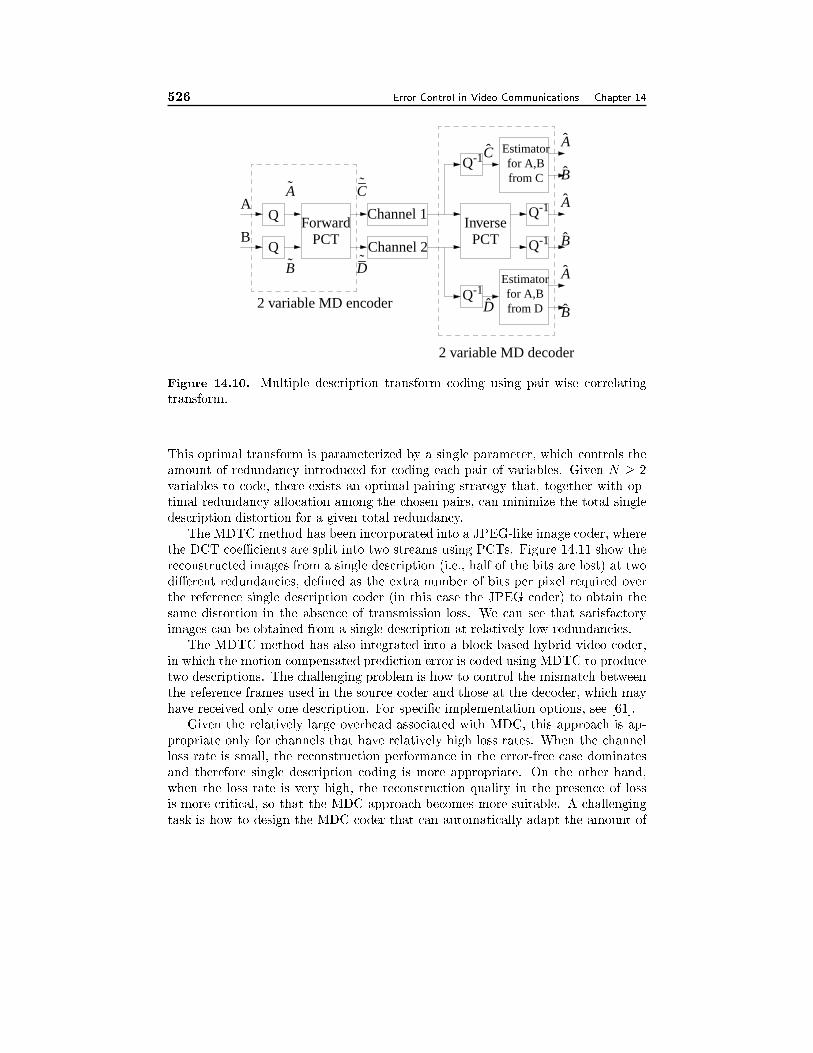
526 Error Control in Video Communications Chapter 14
Q
Q
ForwardPCT
Channel 1
Channel 2
Q-1
Q-1
InversePCT
Q-1
Q-1
Estimatorfor A,Bfrom D
Estimatorfor A,Bfrom C
A
B
2 variable MD encoder
2 variable MD decoder
A
B
A
A
A
B
B
B
C˜
D
C
D
Figure 14.10. Multiple description transform coding using pair-wise correlating
transform.
This optimal transform is parameterized by a single parameter, which controls the
amount of redundancy introduced for coding each pair of variables. Given N � 2
variables to code, there exists an optimal pairing strategy that, together with op-
timal redundancy allocation among the chosen pairs, can minimize the total single
description distortion for a given total redundancy.
The MDTC method has been incorporated into a JPEG-like image coder, where
the DCT coeÆcients are split into two streams using PCTs. Figure 14.11 show the
reconstructed images from a single description (i.e., half of the bits are lost) at two
di�erent redundancies, de�ned as the extra number of bits per pixel required over
the reference single description coder (in this case the JPEG coder) to obtain the
same distortion in the absence of transmission loss. We can see that satisfactory
images can be obtained from a single description at relatively low redundancies.
The MDTC method has also integrated into a block-based hybrid video coder,
in which the motion compensated prediction error is coded using MDTC to produce
two descriptions. The challenging problem is how to control the mismatch between
the reference frames used in the source coder and those at the decoder, which may
have received only one description. For speci�c implementation options, see [61].
Given the relatively large overhead associated with MDC, this approach is ap-
propriate only for channels that have relatively high loss rates. When the channel
loss rate is small, the reconstruction performance in the error-free case dominates
and therefore single description coding is more appropriate. On the other hand,
when the loss rate is very high, the reconstruction quality in the presence of loss
is more critical, so that the MDC approach becomes more suitable. A challenging
task is how to design the MDC coder that can automatically adapt the amount of
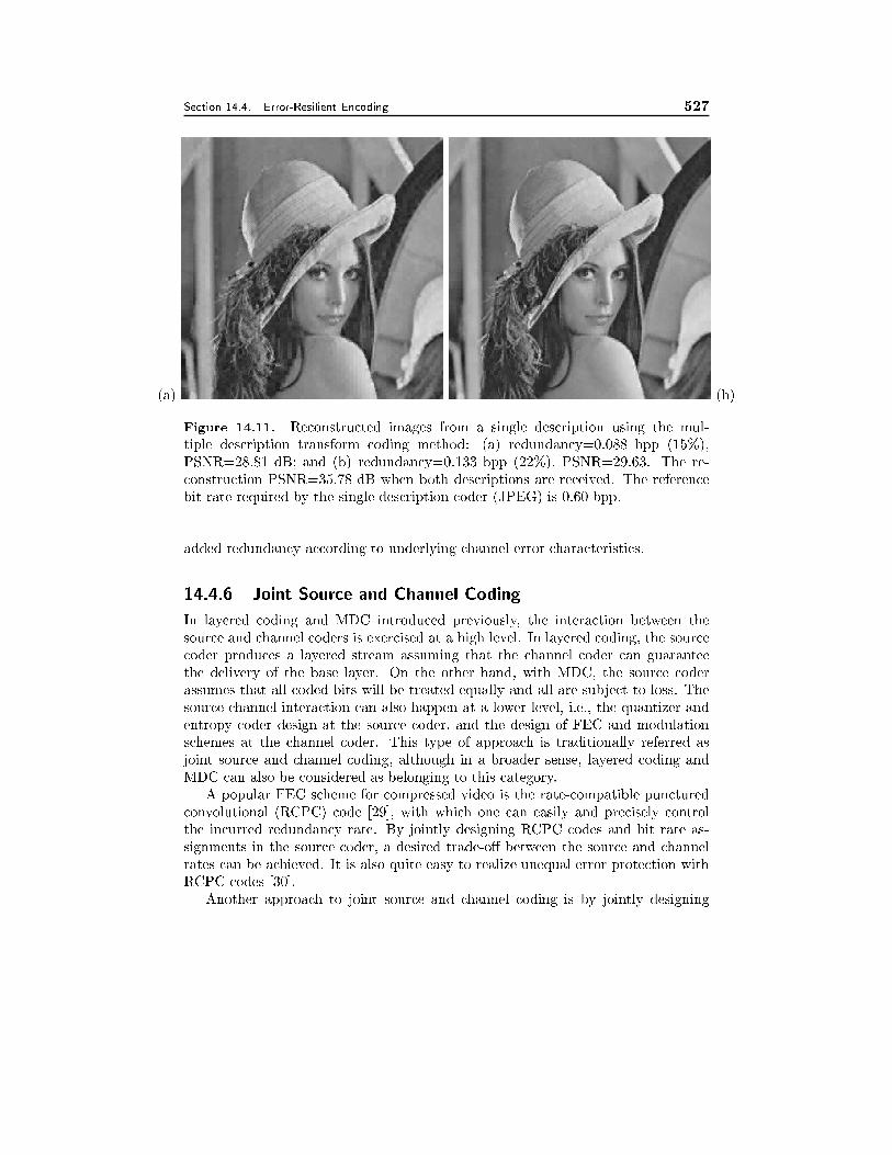
Section 14.4. Error-Resilient Encoding 527
(a) (b)
Figure 14.11. Reconstructed images from a single description using the mul-
tiple description transform coding method: (a) redundancy=0.088 bpp (15%),
PSNR=28.81 dB; and (b) redundancy=0.133 bpp (22%), PSNR=29.63. The re-
construction PSNR=35.78 dB when both descriptions are received. The reference
bit rate required by the single description coder (JPEG) is 0.60 bpp.
added redundancy according to underlying channel error characteristics.
14.4.6 Joint Source and Channel Coding
In layered coding and MDC introduced previously, the interaction between the
source and channel coders is exercised at a high level. In layered coding, the source
coder produces a layered stream assuming that the channel coder can guarantee
the delivery of the base layer. On the other hand, with MDC, the source coder
assumes that all coded bits will be treated equally and all are subject to loss. The
source-channel interaction can also happen at a lower level, i.e., the quantizer and
entropy coder design at the source coder, and the design of FEC and modulation
schemes at the channel coder. This type of approach is traditionally referred as
joint source and channel coding, although in a broader sense, layered coding and
MDC can also be considered as belonging to this category.
A popular FEC scheme for compressed video is the rate-compatible punctured
convolutional (RCPC) code [29], with which one can easily and precisely control
the incurred redundancy rate. By jointly designing RCPC codes and bit rate as-
signments in the source coder, a desired trade-o� between the source and channel
rates can be achieved. It is also quite easy to realize unequal error protection with
RCPC codes [30].
Another approach to joint source and channel coding is by jointly designing
528 Error Control in Video Communications Chapter 14
the quantizer and the binary encoder for given channel error characteristics, to
minimize the e�ect of transmission errors [49, 19, 56, 57, 75, 20, 78]. One can
also carefully design the mapping between quantized source codewords and their
modulation symbols. By assigning close-by points in the modulation constellation
space to close-by source codewords, the e�ect of channel error can be reduced [93,
22].
Note that techniques in this category are mainly targeted at bit errors and are
not very e�ective in communication systems where compressed data are packetized
and packet loss is the dominant contributor to transmission errors.
14.5 Decoder Error Concealment
As mentioned in the previous sections, due to various channel/network errors, com-
pressed video data can be damaged or lost during transmission or storage. In
Sec. 14.3, we described the mechanisms that can be invoked at the transport layer,
to minimize transmission loss. Unless retransmission can be used inde�nitely, which
is unacceptable for real-time applications, there will be remaining errors and losses
in the received data. In Sec. 14.4, we presented various ways that the encoder can
use to suppress the e�ect of such errors. Still, a transmission error may lead to ob-
jectionable visual distortion in the reconstructed signal at the decoder. Depending
on many factors such as source coding, transport protocol, the amount and type of
information loss, etc, the introduced distortion can range from momentary degra-
dation to a completely unusable image or video signal. In this section, we describe
techniques that can be employed at the decoder to conceal the e�ect of transmission
errors, so as to make the decoded signal much less visually objectionable.
Error concealment is possible because, due to various constraints such as coding
delay, implementation complexity and availability of a good source model, a com-
pressed video bitstream still possesses a certain degree of statistical redundancy,
despite the tremendous research e�ort that has been devoted towards achieving the
highest possible compression gain. Also, the source coder may incorporate some of
the error-resilient mechanisms, to intentionally introduce redundancy in the coded
bits, so as to facilitate the estimation of lost data. In addition, the human percep-
tion system can tolerate a limited degree of signal distortion. All these factors can
be exploited for error concealment at the decoder.
Error concealment belongs to the general problem of image recovery or restora-
tion. However, because errors are incurred at the compressed bit level, the resulting
error patterns in the pixel domain are very peculiar and special measures are usually
needed to handle such errors. As described before, because of the use of predictive
coding and VLC, a bit error alone can cause damage to a large region. To contain
the error e�ect, various measures can be taken in the encoder to make the com-
pressed stream more error-resilient, at the expense of a certain degree of coding
gain and/or complexity. Here we assume synchronization codewords are inserted
periodically within a picture (cf. Sec. 14.4.1) and the prediction loop is periodically
reset (cf. Sec. 14.4.3), so that a bit error or packet loss will only cause damage to
Section 14.5. Decoder Error Concealment 529
a limited region in a picture.
Depending on the frequency of synchronization codewords, transport packet size
and bitrate, a damaged region can range from part of a macroblock to an entire
picture. For high bitrate transmission over small packets as in ATM networks,
a lost packet may only damage part of a MB or several adjacent MBs. In this
case, a damaged MB is typically surrounded by multiple undamaged MBs in the
same frame. When this is the case, we can use spatial interpolation to recover the
damaged MB. On the other hand, for low-bitrate application over relatively large
packets (for example, 128 kb/s over IP networks), a lost packet is likely to damage
a large portion of a frame or an entire frame. Under such situations, we have to rely
on the previous and possibly following video frames for concealment of the damaged
frame. Obviously, information from adjacent frames can also be incorporated even
if neighboring MBs are available in the same frame.
Given the block-based hybrid coding paradigm, there are three types of infor-
mation that may need to be estimated in a damaged MB: the texture information,
including the pixel or DCT coeÆcient values for either an original image block or
a prediction error block, the motion information, consisting of MV(s) for a MB
coded in either P- or B-mode, and �nally the coding mode of the MB. The recovery
techniques for these information types are somewhat di�erent.
It is well-known that images of natural scenes have predominantly low frequency
components, i.e., the color values of spatially and temporally adjacent pixels vary
smoothly, except in regions with edges. All the techniques that have been developed
for recovering texture information make use of the above smoothness property of
image/video signals, and essentially they all perform some kind of spatial/temporal
interpolation. The MV �eld, to a lesser extent, also shares the smoothness property,
and can also be recovered by using spatial/temporal interpolation. For the coding
mode information, the methods developed tend to be more driven by heuristics. In
the following subsections, we review some representative techniques for each cate-
gory. More extensive coverage of methods discussed here as well as other methods
can be found in [82, 99, 47]. We will assume that error locations have been de-
tected via other means, such as lost packet detection based on sequence numbers in
services using RTP. For a coverage of various error detection methods, see [82].
Note that in a typical (non-error-resilient) encoder implementation, bits for these
three types of data are stored sequentially for each MB, so that they are all lost in
a damaged block. With the use of data partitioning (Sec. 14.4.1), it is possible that
the coding mode, MV(s), and possibly �rst few DCT coeÆcients are still available
in a damaged block. As can be seen from below, the knowledge of the coding mode
and MV can help the recovery of the texture information greatly.
14.5.1 Recovery of Texture Information
Motion Compensated Temporal Interpolation
The simplest approach to recover a damaged MB is by copying the corresponding
MB in the previously decoded frame. This however will give unsatisfactory results
530 Error Control in Video Communications Chapter 14
if there is a large motion in the scene. A more e�ective solution is to use the MB
in the previous frame pointed to by the MV for the damaged MB. The recovery
performance by this approach is critically dependent on the availability of the MV.
When the MV is also missing, it must �rst be estimated, which is discussed below.
To reduce the impact of the error in the estimated MVs, temporal prediction may
be combined with spatial interpolation (see below).
Spatial Interpolation
Another simple approach is to interpolate pixels in a damaged block from pixels in
adjacent correctly received blocks in the same frame. Usually, all blocks (or MBs)
in the same row are put into the same packet, so that a packet loss typically leads
to the loss of all blocks in a row. In this situation, the only available neighboring
blocks for a damaged block are those above and below. Because most pixels in these
blocks are too far away from the missing samples, usually only the boundary pixels
in neighboring blocks are used for interpolation. Instead of interpolating individual
pixels, a simpler approach is to estimate the DC coeÆcient (i.e. the mean value)
of a damaged block and replace the damaged block by a constant equal to the
estimated DC value. The DC value can be estimated by averaging the DC values
of surrounding blocks. One way to facilitate such spatial interpolation is by using
interleaved packetization (Sec. 14.3.2) so that the loss of one packet will damage
only alternating blocks or MBs.
Maximally Smooth Recovery (MSR)
A problem with spatial interpolation approaches is how to determine appropriate
interpolation �lter. Another shortcoming is that it ignores received DCT coeÆ-
cients, if any. These problems are resolved in the MSR approach of [100, 83] by
requiring the recovered pixels in a damaged block to be smoothly connected with
its neighboring pixels both spatially in the same frame and temporally in the pre-
vious/following frames. If some but not all DCT coeÆcients are received for this
block, then the estimation should be such that the recovered block be as smooth
as possible, subject to the constraint that the DCT on the recovered block would
produce the same values for the received coeÆcients. The above objectives can
be formulated as an optimization problem, and the solutions under di�erent loss
patterns correspond to di�erent interpolation �lters in the spatial, temporal, and
frequency domains.
Spatial Interpolation Using Projection onto Convex Sets (POCS)
Another way of accomplishing spatial interpolation is by using the POCS method
[69, 92]. The general idea behind POCS-based estimation methods is to formulate
each constraint about the unknowns as a convex set. The optimal solution is the
intersection of all the convex sets, which can be obtained by recursively projecting a
previous solution onto individual convex sets. When applying POCS for recovering
an image block, the spatial smoothness criterion is formulated in the frequency
Section 14.5. Decoder Error Concealment 531
domain, by requiring the discrete Fourier transform (DFT) of the recovered block
to have energy only in several low frequency coeÆcients. If the damaged block is
believed to contain an edge in a particular direction, then one can require the DFT
coeÆcients to be distributed along a narrow stripe orthogonal to the edge direction,
i.e., low-pass along the edge direction, and all-pass in the orthogonal direction. The
requirement on the range of each DFT coeÆcient magnitude can also be converted
into a convex set, so is the constraint imposed by any received DCT coeÆcient.
Because the solution can only be obtained through an iterative procedure, this
approach may not be suitable for real-time applications.
14.5.2 Recovery of Coding Modes and Motion Vectors
As already indicated, some of the above algorithms are contingent upon the knowl-
edge of the coding mode and MVs for P- or B-mode MBs. To facilitate decoder
error concealment, the encoder may perform data partition, to pack the mode and
MV information in a separate partition and transmit them with stronger error pro-
tection (cf. Sec. 14.4.1). This for example is an error resilience mode in both H.263
and MPEG-4. Still, the mode and MV information can be damaged.
One way to estimate the coding mode for a damaged MB is by collecting the
statistics of the coding mode pattern of adjacent MBs, and �nd a most likely mode
given the modes of surrounding MBs [68]. A simple and conservative approach,
when the coding mode is lost, is to assume that the MB is coded in the intra-mode,
and use only spatial interpolation for recovering the underlying blocks.
For estimating lost MVs, there are several simple operations [50]: (a) assuming
the lost MVs to be zeros, which works well for video sequences with relatively small
motion; (b) using the MVs of the corresponding MB in the previous frame; (c)
using the average of the MVs from spatially adjacent MB's; (d) using the median of
MVs from the spatially adjacent MB's; (e) re-estimating the MVs [33]. Typically,
when a MB is damaged, its horizontally adjacent MBs are also damaged, and hence
the average or mean is taken over the MVs above and below. A simpler approach
is to use the MV for the MB above the damaged MB. Research has shown that
no signi�cant improvement in picture quality can be achieved when using mean or
median values of more than one MV [81]. To facilitate the estimation of lost MVs,
interleaved packetization (Sec. 14.3.2) can be used. For example, if even and odd
rows of MB's are put into alternating packets, then the loss of a packet will damage
only alternating rows.
14.5.3 Syntax-Based Repair
The previous error concealment techniques work in the signal domain, assuming
that the error in the transmitted stream has been detected, \questionable" data
units have been discarded, and the remaining bits have been decoded into signal
variables (e.g., side information, MV's, DCT coeÆcients) by the VLC decoder.
Syntax-based repair, on the other hands, tries to detect and repair errors in the
bitstream directly. This is possible, because, for any �nite length data packet,
532 Error Control in Video Communications Chapter 14
there is only a relatively small number of valid combinations of codewords. In
addition, a compressed bitstream is never an i.i.d. white binary sequence. The
distribution of 1's and 0's in the bitstream is often location dependent [81]. Based on
such information, the decoder can repair the bitstream so that the repaired stream
conforms to the syntax dictated by the encoding scheme. The use of data partition
and RVLC in H.263 and MPEG-4 helps to perform syntax-based repair, as they
allow more \check points" and syntax constraints, which makes the total number
of valid combinations of codewords smaller than the number of all possible binary
strings of the same length. One such repair scheme, known as \soft-decoding", is
described in [84]. Syntax-based repair is an e�ective error concealment method for a
channel where bit errors dominate. For packet lossy network, where many complete
packets may be lost, syntax-based repair is only used to detect errors in the received
packets, but cannot be used to reconstruct the mission data.
14.6 Encoder and Decoder Interactive Error Control
In the techniques presented thus far, the encoder and decoder operate independently
as far as combating transmission errors is concerned. Conceivably if a backward
channel from the decoder to the encoder is available, better performance can be
achieved if the sender and the receiver cooperate in the process of error control.
This cooperation can be realized at either the source coding or transport level.
At the source coder, coding parameters can be adapted based on the feedback
information from the decoder. At the transport level, the feedback information
can be employed to change the percentage of the total bandwidth used for FEC or
retransmission. We have described transport-level adaptations in Sec. 14.3. In this
section, we describe several techniques that adapt the source coding strategy based
on the feedback information from the decoder. These techniques are developed under
the assumption that it is often acceptable to have errors as long as they do not last
too long. Therefore, even if one cannot a�ord to correct the errors whenever they
occur, it is important to limit the propagation scope of such errors.
Before we proceed to describe these techniques, it is worthwhile to note how is the
feedback information delivered. Typically, the feedback message is not part of the
video syntax but transmitted in a di�erent layer of the protocol stack where control
information is exchanged. For example, in the H.323 standards for multimedia
communications over unreliable channels [43], the control protocol H.245 [41] allows
reporting of the temporal and spatial location of damaged MB's. Usually, such
messages are delivered error-free, by the use of retransmission when necessary.
14.6.1 Coding Parameter Adaptation based on Channel Condi-tions
In a channel with varying bandwidth and error characteristics, it is important to
match the encoding rate with the available channel bandwidth and to embed ap-
propriate error resilience in the coded bit stream. When a source is coded at a rate
Section 14.6. Encoder and Decoder Interactive Error Control 533
higher than the underlying channel can deliver in time, some data will be thrown
away at the discretion of the network layer, typically leading to more disturbing
artifacts than the source coding distortion incurred by encoding the source at a
lower rate. Furthermore, when a channel is very noisy, it is better to represent a
source with lower quality, leaving more bits for error protection either in the form
of FEC or error resilience in the encoded stream.
There are two tasks that must be solved: First the transport controller must be
able to periodically estimate/update the QoS parameters (e.g. bandwidth, delay,
packet loss rates) of an established connection based on the feedback information
or other transport level interactions; Secondly, given the available bandwidth and
error characteristics, the encoder must determine the coding parameters (such as
intra block rate, frequency of synchronization markers, range of prediction, etc. in a
block-based hybrid coder) appropriately so as to meet the target bit rate and desired
amount of error resilience. We have discussed the rate control issue in Sec. 9.3.4,
without considering the error resilence factors. In Sec. 14.4.3, we described several
approaches to coding mode selection (intra. vs. inter) that take into account
loss characteristics of the network. The paper by Wu et al. considers both rate
estimation and rate adaptation for video delivery over Internet [90]. More on how
to adjust the target encoding rate based on channel feedback for the application of
video streaming over the Internet is discussed in Sec.15.3.1.
14.6.2 Reference Picture Selection based on Feedback Informa-tion
One way of taking advantage of an available feedback channel is to employ reference
picture selection (RPS). If the encoder learns through a feedback channel about
damaged parts of a previously coded frame, it can decide to code the next P-frame
not relative to the most recent, but to an older reference picture, which is known to
be available in the decoder. This requires that the encoder and decoder both store
multiple past decoded frames. Information about the reference picture to be used is
conveyed in the bitstream. Compared to coding the current picture as an I-frame,
the reduction in the coding eÆciency due to use of an older reference picture is
signi�cantly lower, if the reference picture is not too far away. A study on the delay
and overhead incurred by using RPS can be found in [26].
Note that using RPS does not necessarily mean extra delay in the encoder. The
encoder does not have to wait for the arrival of the feedback information about the
previous frame to code a current frame. Rather, it can choose to use as reference
a frame before the damaged frame whenever it receives the feedback information.
For example, if the information about the damage of frame n does not arrive at the
encoder until the time to code frame n + d, the decoded frames between n + 1 to
n+ d� 1 would all have errors, because the decoder uses di�erent reference frames
than the encoder for these frames. By selecting frame n� 1 as the reference frame
to code frame n+ d, error propagation will be stopped from frame n+ d onwards.
Of course, the longer it takes to generate and deliver the feedback information, the
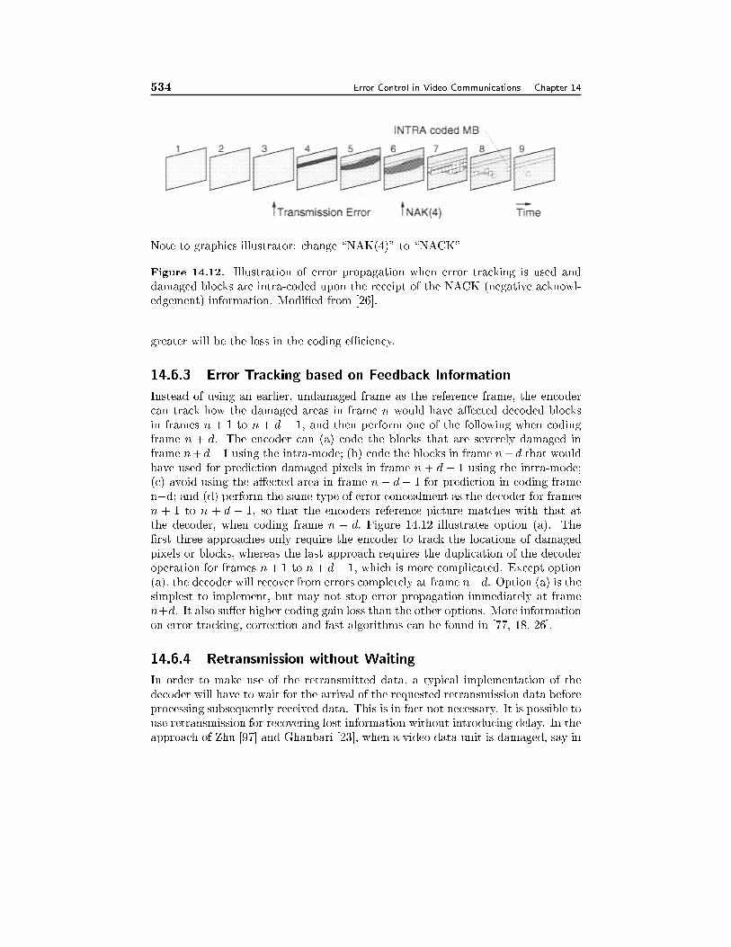
534 Error Control in Video Communications Chapter 14
Note to graphics illustrator: change \NAK(4)" to \NACK"
Figure 14.12. Illustration of error propagation when error tracking is used and
damaged blocks are intra-coded upon the receipt of the NACK (negative acknowl-
edgement) information. Modi�ed from [26].
greater will be the loss in the coding eÆciency.
14.6.3 Error Tracking based on Feedback Information
Instead of using an earlier, undamaged frame as the reference frame, the encoder
can track how the damaged areas in frame n would have a�ected decoded blocks
in frames n + 1 to n + d � 1, and then perform one of the following when coding
frame n + d. The encoder can (a) code the blocks that are severely damaged in
frame n+d�1 using the intra-mode; (b) code the blocks in frame n+d that would
have used for prediction damaged pixels in frame n + d � 1 using the intra-mode;
(c) avoid using the a�ected area in frame n+ d � 1 for prediction in coding frame
n+d; and (d) perform the same type of error concealment as the decoder for frames
n + 1 to n + d � 1, so that the encoders reference picture matches with that at
the decoder, when coding frame n + d: Figure 14.12 illustrates option (a). The
�rst three approaches only require the encoder to track the locations of damaged
pixels or blocks, whereas the last approach requires the duplication of the decoder
operation for frames n+ 1 to n+ d� 1; which is more complicated. Except option
(a), the decoder will recover from errors completely at frame n+d. Option (a) is the
simplest to implement, but may not stop error propagation immediately at frame
n+d. It also su�er higher coding gain loss than the other options. More information
on error tracking, correction and fast algorithms can be found in [77, 18, 26].
14.6.4 Retransmission without Waiting
In order to make use of the retransmitted data, a typical implementation of the
decoder will have to wait for the arrival of the requested retransmission data before
processing subsequently received data. This is in fact not necessary. It is possible to
use retransmission for recovering lost information without introducing delay. In the
approach of Zhu [97] and Ghanbari [23], when a video data unit is damaged, say in
Section 14.7. Error Resilience Tools in H.263 and MPEG-4 535
frame n, a retransmission request is sent to the encoder for recovering the damaged
data. Instead of waiting for the arrival of retransmitted data, the damaged video
part is concealed by a chosen error concealment method. Then normal decoding
is continued, while a trace of the a�ected pixels and their associated coding infor-
mation (coding mode and motion vectors) is recorded (similar to the error tracking
method described in Sec. 14.6.3). Upon the arrival of the retransmitted data, say
at frame n + d, the a�ected pixels are corrected, so that they are reproduced as
if no transmission loss had occurred. The correction signal is obtained from the
retransmitted data and the recorded trace.
This method can achieve lossless recovery except during the time between the in-
formation loss and the arrival of the retransmission data. During that interval, any
error concealment technique (Sec. 14.5) can be applied to the damaged regions. This
scheme eliminates the delay associated with conventional retransmission schemes
without compromising the video quality. The price paid is the relatively high im-
plementation complexity. Compared to the error tracking approach in Sec. 14.6,
which adapts encoding operation to stop error propagation, the current approach
makes use of retransmitted data to correct and stop error at the decoder.
14.7 Error Resilience Tools in H.263 and MPEG-4
In this section, we summarize the error resilience tools de�ned in the H.263 and
MPEG-4 standards as options. These tools fall in the error-resilient encoding cate-
gory, even though the standards only de�ne the bitstream syntax. It is worth noting
that, as with any error-resilient encoding methods, these tools tend to reduce the
coding eÆciency slightly. However, they give a good decoder the tools to localize
errors in the bitstream, to limit the image area that gets a�ected by these errors,
and to apply appropriate error concealment methods (Sec. 14.5). How these tools
are used to help the decoder operation is outside the scope of the standard, which
enables competition between di�erent decoder vendors.
14.7.1 Error Resilience Tools in ITU-T H.263
The initial target of the H.263 standard was to serve as a video coding standard for
the H.324 system, which aims to enable video telephony over wireline and wireless
modems. As described in Sec. 14.2, by applying appropriate FEC and multiplex-
ing, both the wireline and wireless modem channels can be considered error-free.
Therefore the initial focus of the H.263 development was on enhancing the coding
eÆciency only. As the H.323 standard develops, which targets primarily at video
telephony and conferencing over the best e�ort Internet, the error resilience issues
become a major concern. A set of annexes were developed to augment the previous
H.263 standard. The following are the error resilience tools included in Version 3
of the H.263 standard (i.e., H.263++), which is approved November 2000.
Forward Error Correction Using BCH Code (Annex H): This tool allows in-
cluding, for blocks of 492 coded video bits, a 19 bit BCH (511, 492) FEC parity
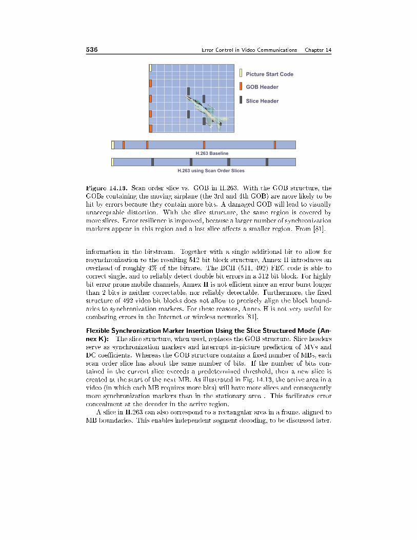
536 Error Control in Video Communications Chapter 14
Picture Start Code
GOB Header
Slice Header
H.263 Baseline
H.263 using Scan Order Slices
Figure 14.13. Scan order slice vs. GOB in H.263. With the GOB structure, the
GOBs containing the moving airplane (the 3rd and 4th GOB) are more likely to be
hit by errors because they contain more bits. A damaged GOB will lead to visually
unacceptable distortion. With the slice structure, the same region is covered by
more slices. Error resilience is improved, because a larger number of synchronization
markers appear in this region and a lost slice a�ects a smaller region. From [81].
information in the bitstream. Together with a single additional bit to allow for
resynchronization to the resulting 512 bit block structure, Annex H introduces an
overhead of roughly 4% of the bitrate. The BCH (511, 492) FEC code is able to
correct single, and to reliably detect double bit errors in a 512 bit block. For highly
bit error prone mobile channels, Annex H is not eÆcient since an error burst longer
than 2 bits is neither correctable, nor reliably detectable. Furthermore, the �xed
structure of 492 video bit blocks does not allow to precisely align the block bound-
aries to synchronization markers. For these reasons, Annex H is not very useful for
combating errors in the Internet or wireless networks [81].
Flexible Synchronization Marker Insertion Using the Slice Structured Mode (An-
nex K): The slice structure, when used, replaces the GOB structure. Slice headers
serve as synchronization markers and interrupt in-picture prediction of MVs and
DC coeÆcients. Whereas the GOB structure contains a �xed number of MBs, each
scan order slice has about the same number of bits. If the number of bits con-
tained in the current slice exceeds a predetermined threshold, then a new slice is
created at the start of the next MB. As illustrated in Fig. 14.13, the active area in a
video (in which each MB requires more bits) will have more slices and consequently
more synchronization markers than in the stationary area . This facilitates error
concealment at the decoder in the active region.
A slice in H.263 can also correspond to a rectangular area in a frame, aligned to
MB boundaries. This enables independent segment decoding, to be discussed later.
Section 14.7. Error Resilience Tools in H.263 and MPEG-4 537
Reference Picture Selection (RPS) (Annex N and Annex U): As introduced in
Sec. 14.6.2, RPS enables the encoder to use, for motion compensation, an older
reference picture that is known to be correctly received at the decoder's site. In
H.263, RPS can be used on whole pictures, picture segments (slices or GOBs), or on
individual MBs. The former two mechanisms are de�ned in Annex N and were in-
troduced as an error resilience tool only, whereas the latter, de�ned in Annex U, was
designed with both error resilience and coding eÆciency in mind.4 In H.263, RPS
can be used with or without feedback information. Without feedback information,
the video redundancy coding method described in Sec. 14.4.3 can be used, which
employs a pre�xed interleaved reference picture selection scheme. This technique
is, however, much less eÆcient than feedback-based mechanisms [87, 88].
Scalability (Annex O): Annex O de�nes temporal, spatial, and SNR scalability
similar to those used in MPEG-2. As described in Sec. 14.4.4, these tools can be
used to enhance the error resilience if multiple transport paths with di�erent QoS
characteristics are available between the source and the destination.
Independent Segment Decoding (ISD) (Annex R): ISD forces encoder and de-
coder to treat segment (slice or GOB) boundaries like picture boundaries, thereby
preventing the propagation of corrupted data in one segment to another. This
method is a special case of error-resilient prediction discussed in Sec. 14.4.3. ISD
in conjunction with rectangular slices has been shown to improve error resilience
[88]. The overhead of ISD is roughly reversely proportional to the picture size, and
is impractically high for picture sizes smaller than CIF [81].
Data Partitioning and RVLC (Annex V): As already introduced, with data par-
titioning, MB header, MV, and DCT information are no longer interleaved on a
MB by MB basis, rather, they are grouped into separate partitions separated with
specially designed markers. Header and motion information is coded with RVLC,
whereas the DCT coeÆcients are coded using the non-reversible VLC table used in
the baseline H.263.
Header Repetition (Annex W): This allows the repetition of the header of the
previous frame in the header of the current frame. This enables, with a frame delay,
the decoding of a frame for which the frame header is lost. Note that H.263 contains
no syntax element that allows including redundant picture header information at
the slice level, as is available in MPEG-4's Header Extension Code (see Sec. 14.7.2).
For a discussion on how the above tools can be incorporated in a video codec
for video transmission over the Internet and wireless networks, see [81].
14.7.2 MPEG-4
One of the primary objectives of the MPEG-4 standard is to enable universal access.
Therefore, error resilience is an important issue to consider from the very beginning.
4By allowing an MB to choose the best matching MB among a set of past frames, the coding
eÆciency can be increased at the expense of motion estimation complexity.
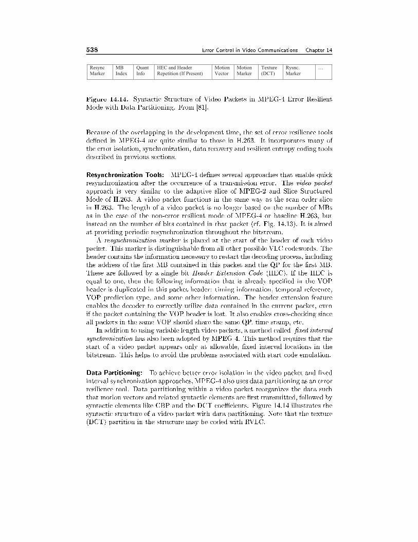
538 Error Control in Video Communications Chapter 14
Resync
Marker
MB
Index
Quant
Info
HEC and Header
Repetition (If Present)
Motion
Vector
Motion
Marker
Texture
(DCT)
Rysnc.
Marker
…
Figure 14.14. Syntactic Structure of Video Packets in MPEG-4 Error Resilient
Mode with Data Partitioning. From [81].
Because of the overlapping in the development time, the set of error resilience tools
de�ned in MPEG-4 are quite similar to those in H.263. It incorporates many of
the error isolation, synchronization, data recovery and resilient entropy coding tools
described in previous sections.
Resynchronization Tools: MPEG-4 de�nes several approaches that enable quick
resynchronization after the occurrence of a transmission error. The video packet
approach is very similar to the adaptive slice of MPEG-2 and Slice Structured
Mode of H.263. A video packet functions in the same way as the scan order slice
in H.263. The length of a video packet is no longer based on the number of MBs
as in the case of the non-error resilient mode of MPEG-4 or baseline H.263, but
instead on the number of bits contained in that packet (cf. Fig. 14.13). It is aimed
at providing periodic resynchronization throughout the bitstream.
A resynchronization marker is placed at the start of the header of each video
packet. This marker is distinguishable from all other possible VLC codewords. The
header contains the information necessary to restart the decoding process, including
the address of the �rst MB contained in this packet and the QP for the �rst MB.
These are followed by a single bit Header Extension Code (HEC). If the HEC is
equal to one, then the following information that is already speci�ed in the VOP
header is duplicated in this packet header: timing information, temporal reference,
VOP prediction type, and some other information. The header extension feature
enables the decoder to correctly utilize data contained in the current packet, even
if the packet containing the VOP header is lost. It also enables cross-checking since
all packets in the same VOP should share the same QP, time stamp, etc.
In addition to using variable length video packets, a method called �xed interval
synchronization has also been adopted by MPEG-4. This method requires that the
start of a video packet appears only at allowable, �xed interval locations in the
bitstream. This helps to avoid the problems associated with start code emulation.
Data Partitioning: To achieve better error isolation in the video packet and �xed
interval synchronization approaches, MPEG-4 also uses data partitioning as an error
resilience tool. Data partitioning within a video packet reorganizes the data such
that motion vectors and related syntactic elements are �rst transmitted, followed by
syntactic elements like CBP and the DCT coeÆcients. Figure 14.14 illustrates the
syntactic structure of a video packet with data partitioning. Note that the texture
(DCT) partition in the structure may be coded with RVLC.
Section 14.8. Summary 539
NEWPRED mode: This tool is very similar to the H.263 RPS Mode (Annex
N) and the Slice Structured Mode (Annex K). When the NEWPRED mode is
turned on, the reference used for inter prediction by the encoder will be updated
adaptively according to the feedback messages from the decoder. These messages
indicate which NEWPRED (ND) segments (which can either be an entire frame,
or in MPEG-4 language, a VOP, or the content of a packet, typically one slice)
have been successfully decoded, and which ND segments have not. Based on the
feedback information the encoder will either use the most recent ND segment, or a
spatially corresponding but older ND segment for prediction.
Data Recovery in Conjunction with RVLC and Data Partitioning: The MPEG-4
error resilience mode utilizes RVLC for better recovery of DCT data. The usage
of RVLC is signaled at the Video Object Layer (VOL). When RVLC is used for
DCT data, the bitstream is decoded in the forward direction �rst. If no errors are
detected, the bitstream is assumed to be valid. If an error is detected however,
two-way decoding is applied, and the portion of the packet between the �rst MB
in which an error was detected in both the forward and backward directions should
not be used.
14.8 Summary
In this chapter, we described various error-control mechanisms that can be used
to combat transmisson errors in real-time video communications. We focused on
techniques developed for block-based hybrid coders, especially those that have been
adopted in the H.263 and MPEG-4 standards. The key features of di�erent cate-
gories of error-control techniques are summarized below.
Transport-Level Error Control
Transport-level error control mechanisms are most important and guarantees a basic
level of quality. Error control can be applied through FEC, interleaved packetiza-
tion, and when feasible, properly constrained retransmission. Di�erent levels of
protection can be applied to parts of coded bits that are of varying importance.
Such unequal error protection is an e�ective way of employing a limited amount of
redundancy to achieve acceptable quality.
Error-Resilient Encoding
Techniques in this category achieve error resilience by adding a certain amount
of redundancy in the coded bit streams at the source coder. Some are aimed at
guaranteeing a basic level of quality and providing a graceful degradation upon
the occurrence of transmission errors (e.g. layered coding and MDC), some help
to prevent error propagation (e.g. error-resilient prediction), while others help to
detect or recover from bit errors (e.g. error isolation and robust entropy coding).
Some techniques require close interaction between the source coder and transport
540 Error Control in Video Communications Chapter 14
layer (e.g., layered coding with unequal error protection, error resilient prediction
with interleaved packetization), while others assume that di�erent substreams are
treated equally in the transport layer (e.g., MDC). Note that some techniques (error
isolation, RVLC, joint source and channel coding as described in Sec. 14.4.6) are
only useful for combating bit errors and are not helpful for recovering from packet
loss.
Decoder Error Concealment
All the error concealment techniques for texture recover the lost information by
making use of the temporal and spatial smoothness property of image and video
signals. The MSR technique enforces the smoothness constraint by minimizing the
roughness of the reconstructed signal. The motion-compensated temporal inter-
polation method and spatial interpolation method can be considered as a special
case of the MSR approach when only the temporal or spatial di�erence measure is
minimized. The POCS method, on the other hand, iteratively projects the recon-
structed image block onto the convex sets determined by the received coeÆcients
and the smoothness constraint determined from the estimated edge direction of the
block. Although generally giving more accurate results than the MSR, the POCS
method is computationally more intensive, as it requires many iterations. Simple
and yet e�ective, motion-compensated temporal interpolation has been employed in
commercial systems. More complex methods that exploit spatial correlation (spa-
tial interpolation, MSR and POCS) can o�er additional improvement only when
the underlying scene has very complex motion or is experiencing scene changes.
Recovery of coding mode and motion information is more diÆcult than the
texture information, because there are less correlation among the coding modes
and motion vectors of adjacent MB's. When possible, such information should
be more heavily protected than the texture information, through the use of data
partitioning and unequal error protection.
Encoder and Decoder Interactive Error Control
Such techniques are applicable when there is a backward channel from the decoder
to the encoder so that the decoder can inform the encoder which part of the coded
information is lost. The three techniques presented, reference picture selection,
error tracking, and retransmission without waiting, all aim to stop error propagation
after the feedback information is received. The �rst two methods, reference picture
selection and error tracking, avoid using damaged regions for future prediction at the
encoder, while the third, retransmission without waiting, correct the error based on
the retransmitted information. When only a general information about, say packet
loss rate, is available, but not which part of the information is lost, one can try to
adjust the coding parameters so as to reduce data loss and to suppress the e�ect of
any lost data.
Section 14.9. Problems 541
Choice of Di�erent Techniques
Transport-level error control mechanisms are most important and guarantees a ba-
sic level of quality. Error resilient encoding and decoder error concealment are
necessary to further improve the quality in very lossy environments such as the
Internet and wireless networks. Depending on channel error characteristics, system
con�guration and requirements, some techniques are more e�ective than others.
The burstiness of transmission errors has a signi�cant impact on the choice of al-
gorithms. For a channel with very long bursts, error-resilient encoding techniques
may not be appropriate. This is because the redundancy introduced in such coding
methods is wasted when the channel is error-free, and such redundancy is not very
helpful when a burst error occurs. Retransmission, when properly constrained, may
be more suitable since it only introduces the overhead when needed. The existence
of a backward channel from the decoder to the encoder also a�ects the deployment
of some schemes. In applications such as broadcast where there is no backward
channel, none of the interactive error control techniques can be applied. Similarly,
in video streaming applications, videos are usually pre-compressed and stored in
a server, so that it is not possible to adapt encoder operations based on network
conditions. The error concealment techniques can be applied in any circumstances.
However, the e�ectiveness of such techniques is limited by the available information.
Also some techniques may be either too complicated for cost e�ective implemen-
tation or introduce unacceptable processing delay for real-time applications. Aside
from the delay and complexity issues, one important criterion for comparing di�er-
ent schemes is the required redundancy in the source coder and/or the transport
layer, to achieve the same degree of error protection.
14.9 Problems
14.1 What are the main di�erences in the requirements for transporting audio and
video vs. data �les?
14.2 What is the typical delay requirement for an interactive video conferencing
application? What about video streaming?
14.3 What are the contributing factors to the end-to-end delay between a video
source and the displayed video at the receiver?
14.4 We divided the approaches for error control in video communications into four
categories. What are they? Describe the advantages and limitations of each.
14.5 What are the major di�erences between circuit-switching networks and packet-
based networks? What would you choose as your error control mechanisms in
either case?
14.6 What are the major di�erence between LC and MDC? How do they di�er in
terms of network requirements? Describe network conditions under which LC
542 Error Control in Video Communications Chapter 14
may be preferred over MDC, and vice verse.
14.7 What would you do di�erently in the implementation for motion compen-
sated prediction, if the network changed from reliable (almost error free) to
unreliable (with high packet losses)?
14.8 In principle, lost information is un-recoverable. What make error concealment
techniques feasible for video?
14.9 What are the major assumptions in error concealment techniques for recover-
ing damaged texture data?
14.10 Describe the principle of maximally smooth recovery method and the POCS
method for error concealment. What are the pros and cons of each?
14.11 Consider an Internet video conferencing application. Assume the compressed
video streams are packetized, and that a packet is either lost (due to over long
delay or mis-delivery or detected bit errors within a packet) or received intact.
Assume that the e�ective packet loss rate is quite high, about 10%, and that
there is no feedback channel available. The average end-to-end delay between
the source and destination is about 50 ms. Further assume that the maximum
end-to-end delay allowed between the source and destination is 150 ms. What
would you propose as mechanisms to control and conceal the e�ect of packet
loss? What approaches described in this chapter would not be applicable or
e�ective?
14.12 Consider the previous scenario again, but assume that the network has a
lower packet loss rate, say 1%. Would your solution be di�erent?
14.13 Again, consider the scenario in Prob. 14.11, but assume this time that a
feedback channel is available between the destination and the source and that
it usually takes 50 ms to deliver a feedback message. What are the solutions
you propose in this case? What would you send on the feedback channel?
14.14 Now consider video transport over a wireless network with high bit error
rates and bursty errors and narrow bandwidth (say 64 Kbps). You have the
choice to further examine a packet even if the network or decoder has detected
bit errors within a packet based on the FEC code. What are the solutions you
propose in this case? Compared to the Internet case, would you use a shorter
or longer packet?
14.10 Bibliography
[1] R. Aravind, M. R. Civanlar, and A. R. Reibman. Packet loss resilience of
MPEG-2 scalable video coding algorithms. IEEE Trans. Circuits Syst. for Video
Technology, 6(5):426{435, Oct. 1996.
Section 14.10. Bibliography 543
[2] E. Ayanoglu, R. Pancha, A. R. Reibman, and S. Talwar. Forward error con-
trol for MPEG-2 video transport in a wireless ATM LAN. ACM/Baltzer Mobile
Networks and Applications, 1(3):245{258, Dec. 1996.
[3] A. W. Berger. ATM networks. In M. T. Sun and A. R. Reibman, editors,
Compressed Video over Networks. Marcel Dekker, Inc., 2001.
[4] S. Blake, D. Black, M. Carlson, E. Davies, Z. Wang, and W. Weiss. An ar-
chitecture for di�erentiated services, IETF RFC2475, Dec. 1998. Available at
http://www.ietf.org/rfc/rfc2475.txt.
[5] Z. S. Bojkovic and K. R. Rao. Packet Video Communications over ATM Net-
works. Prentice Hall, 2000.
[6] J. C. Bolot, H. Crepin, and A. Vega-Garcia. Analysis of audio packet loss in the
Internet. In Proc. Of the 5th International Workshop on Network and Operating
System Support for Digital Audio and Video, pages 163{174, Durham, April 1995.
[7] C. Bormann, L. Cline, G. Deisher, T. Gardos, C. Maciocco, D. Newell, J. Ott,
G. Sullivan, S. Wenger, and C. Zhu. RTP payload format for the 1998 version of
ITU-T recommendation H.263 video (H.263+), IETF RFC2429, Oct. 1998.
[8] M. Budagavi, W. Rabiner Heinzelman, J. Webb, and R. Talluri. Wireless
MPEG-4 video communiction on DSP chips. IEEE Signal Processing Magazine,
17:36{53, Jan. 2000.
[9] L.-F. Chang. Wireless systems and networking. In M. T. Sun and A. R. Reib-
man, editors, Compressed Video over Networks. Marcel Dekker, Inc., 2001.
[10] K. Chapplapali et al. The grand alliance system for US HDTV. Proc. IEEE,
83(2):158{174, Feb. 1995.
[11] D. Chung and Y. Wang. Multiple description image coding using signal decom-
position and reconstruction based on lapped orthogonal transforms. IEEE Trans.
Circuits Syst. for Video Technology, 9(6):895{908, Sept. 1999.
[12] D. Chung and Y. Wang. Basis design for LOT-based multiple description
coding. In IEEE Int. Conf. Image Proc. (ICIP2000), Vancouver, Canada, Sept.
2000.
[13] M. R. Civanlar. Internet video. In M. T. Sun and A. R. Reibman, editors,
Compressed Video over Networks. Marcel Dekker, Inc., 2001.
[14] M. R. Civanlar and G. L. Cash. A practical system for MPEG-2 based video-
on-demand over ATM packet networks and the WWW. Signal Processing: Image
Commun., 8(3):221{227, 1996.
[15] M. R. Civanlar, G. L. Cash, and B. G. Haskell. RTP payload format for
boundled MPEG, IETF RFC2343, May 1998.
544 Error Control in Video Communications Chapter 14
[16] D. E. Comer. Internetworking with TCP/IP. Prentice Hall, 1995.
[17] G. Cot�e, S. Shirani, and F. Kossentini. Optimal mode selection and synchro-
nization for robust video communications over error prone networks. IEEE Journal
on Selected Areas in Communications, 18(6):952{965, June 2000.
[18] E. Steinbach and N. F�arber and B. Girod. Standard compatible extension of
H.263 for robust video transmission in mobile environments. IEEE Trans. Circuits
Syst. for Video Technology, 7:872{881, Dec. 1997.
[19] N. Farvardin and V. Vaishampayan. Optimal quantizer design for noisy chan-
nels: an approach to combined source-channel coding. IEEE Trans. Inform. The-
ory, 38:827{838, Nov. 1987.
[20] T. R. Fischer. Joint trellis coded quantization/modulation. IEEE Trans. Com-
mun., 39:172{176, Feb. 1991.
[21] M. Fleming and M. E�ros. Generalized multiple description vector quantiza-
tion. In Data Compression Conference (DCC99), Salt Lake, UT, Mar. 1999.
[22] A. Fuldseth and T. A. Ramstad. Combined video coding and multilevel modu-
lation. In Int. Conf. Image Processing (ICIP'96), pages 77{80, Lausanne, Switzer-
land, Sept. 1996.
[23] M. Ghanbari. Postprocessing of late cells for packet video. IEEE Trans. Circuits
Syst. for Video Technology, 6(6):669{678, Dec. 1996.
[24] H. Gharavi and S. M. Alamouti. Multipriority video transmission for third-
generation wireless communication systems. Proc. IEEE, 87:1751{1763, Oct. 1999.
[25] B. Girod and N. F�arber. Wireless video. In M. T. Sun and A. R. Reibman,
editors, Compressed Video over Networks. Marcel Dekker, Inc., 2001.
[26] B. Girod and N. F�arber. Feedback-based error control for mobile video trans-
mission. Proc. IEEE, 87:1707{1723, Oct. 1999. Special Issue on Video for Mobile
Multimedia.
[27] D. J. Goodman. Wireless personal communications systems. Addison-Wesley,
1997.
[28] V. K. Goyal, J. Kovacevic, R. Arean, and M. Vetterli. Multiple description
transform coding of images. In IEEE Int. Conf. Image Proc. (ICIP98), volume 1,
pages 674{678, Chicago, IL, Oct. 1998.
[29] J. Hagenauer. Rate compatible punctured convolutional codes (RCPC codes)
and their applications. IEEE Trans. Commun., 36:389{399, Apr. 1988.
[30] J. Hagenauer and T. Stockhammer. Channel coding and transmission aspects
for wireless multimedia. Proc. IEEE, 87(10):1764{1777, Apr. 1988.
Section 14.10. Bibliography 545
[31] L. Hanzo. Bandwidth eÆcient wireless multimedia communications. Proc.
IEEE, 86:1342{1382, July 1998.
[32] D. Ho�man, G. Fernando, V. Goyal, and M. R. Civanlar. RTP payload format
for MPEG1/MPEG2 video, IETF RFC2250, Jan. 1998.
[33] M.C. Hong, L. Kondi, H. Scwab, and A. K. Katsaggelos. Video error conceal-
ment techniques. Signal Processing: Image Commun., 14:437{492, 1999. special
issue on Error Resilient Video.
[34] A. Ingle and V. A. Vaishampayan. DPCM system design for diversity systems
with applications to packetized speech. IEEE Trans. Speech and Audio Processing,
3: 48{57, Jan. 1995.
[35] ITU-T. Recommendation H.261: Video codec for audiovisual services at px64
kbits, 1993.
[36] ITU-T. Recommendation H.324: Terminal for low bitrate multimedia commu-
nication, 1995.
[37] ITU-T. Recommendation G.114: General characteristics of international tele-
phone connections and international telephone circuits one way transmission time,
1996.
[38] ITU-T. Recommendation H.223: Multiplexing protocol for low bit rate multi-
media communication, 1996.
[39] ITU-T. Recommendation H.221: Frame structure for a 64 to 1920 kbit/s
channel in audiovisual teleservices, 1997.
[40] ITU-T. Recommendation H.320: Narrow-band visual telephone systems and
terminal equipment, 1997.
[41] ITU-T. Recommendation H.245: Control protocol for multimedia communica-
tion, 1998.
[42] ITU-T. Recommendation H.263: Video coding for low bit rate communication,
1998.
[43] ITU-T. Recommendation H.323: Packet-based multimedia communciations
systems, 1998.
[44] H. Jafarkhani and V. Tarokh. Multiple description trellis coded quantization.
In IEEE Int. Conf. Image Proc. (ICIP98), Chicago, IL, Oct, 1998.
[45] W. Jiang and A. Ortega. Multiple description coding via polyphase transform
and selective quantization. In SPIE Conf. Image Proc. Visual Comm. (VCIP99),
Feb. 1999.
546 Error Control in Video Communications Chapter 14
[46] M. Kansari et al. Low bit rate video transmission over fading channels for
wireless microcellular systems. IEEE Trans. Circuits Syst. for Video Technology,
6:1{11, Feb. 1996.
[47] A. K. Katsaggelos and N. P. Galatsanos, editors. Signal Recovery Techniques
for Image and Video Compression and Transmission. Kluwer Academic Publishers,
1998.
[48] T. Kawahara and S. Adachi. Video transmission technology with e�ective error
protection and tough synchronization for wireless channels. In Proc. ICIP96, pages
101{104, Laussanne, Switzerland, Nov. 1996.
[49] J. Kurtenbach and P. A. Wintz. Quantizing for noisy channels. IEEE Trans.
Commun., 17:291{302, Apr. 1969.
[50] W.-M. Lam, A. R. Reibman, and B. Liu. Recovery of lost or erroneously
received motion vectors. In ICASSP93, pages V417{V420, Minneapolis, Apr. 1993.
[51] S. H. Lee, P. J. Lee, and R. Ansari. Cell loss detection and recovery in variable
rate video. In 3rd Int. Workshop on Packet Video, Morriston, NJ, Mar. 1990.
[52] S. Lin and D. J. Costello. Error Control Coding: Fundamentals and Applica-
tions. Prentice Hall, 1983.
[53] R. Marasli, P. D. Amer, and P. T. Conrad. Retransmission-based partially
reliable transport service: an analytic model. In IEEE Infocomm'96, pages 621{
628, San Francisco, 1996.
[54] K. Maxwell. Asymmetric digital subscriber line: interim technology for the
next forty years. IEEE Commun. Mag., pages 100{106, Oct. 1996.
[55] D. C. Mead. Direct broadcast satellite communications: An MPEG enabled
service. Prentice Hall, 2000.
[56] J. W. Modestino and D. G. Daut. Combined source-channel coding of images.
IEEE Trans. Commun., 7:1644{1659, Nov. 1979.
[57] J. W. Modestino, D. G. Daut, and A. L. Vickers. Combined source-channel cod-
ing of images using the block cosine transform. IEEE Trans. Commun., 29:1261{
1273, Sept. 1981.
[58] A. Ortega and K. Ramchandran. Rate-distortion methods for image and video
compression. IEEE Signal Processing Magazine, 15:23{50, Nov. 1998.
[59] G. Ramamurthy and D. Raychaudhuri. Performance of packet video with
combined error recovery and concealment. In IEEE Infocomm'95, pages 753{761,
1995.
Section 14.10. Bibliography 547
[60] D. W. Redmill and N. G. Kingsbury. The EREC: An error resilient technique
for coding variable- length blocks of data. IEEE Trans. Image Proc., 5(4):565{574,
Apr. 1996.
[61] A. Reibman, H. Jafarkhani, Y. Wang, and M. Orchard. Multiple description
coding for video using motion compensated prediction. In IEEE Int. Conf. Image
Proc. (ICIP99), Kobe, JAPAN, Oct, 1999.
[62] H. Schulzrinne. IP networks. In M. T. Sun and A. R. Reibman, editors,
Compressed Video over Networks. Marcel Dekker, Inc., 2001.
[63] H. Schulzrinne, S. Casner, R. Frederick, and V. Jacobson. RTP: A trans-
port protocol for real-time applications. RFC 1889, IETF, available from
ftp://ftp.isi.edu/in-notes/rfc1889.txt, January 1996.
[64] B. C. Smith. Implementation Techniques for Continuous Media Systems and
Applications. PhD thesis, Univ. California, Berkeley, 1994.
[65] M. Srinivasan and R. Chellappa. Multiple description subband coding. In
IEEE Int. Conf. Image Proc. (ICIP98), Chicago, IL, Oct, 1998.
[66] W. Stallings. ISDN and broadband ISDN. Macmillan Publishing Company,
2nd edition, 1992.
[67] K. Stuhlmuller, N. F�arber, M. Link, and B. Girod. Analysis of video trans-
mission over lossy channels. IEEE Journal on Selected Areas in Communications,
18(6):996{1011, June 2000.
[68] H. Sun, K. Challapali, and J. Zdepski. Error concealment in digital simulcast
AD-HDTV decoder. IEEE Trans. Consumer Electronics, 38(3):108{117, Aug.
1992.
[69] H. Sun and W. Kwok. Concealment of damaged block transform coded images
using projections onto convex sets. IEEE Trans. Image Process., 4(4):470{477,
Apr. 1995.
[70] H. Sun and J. Zdepski. Error concealment strategy for picture-header loss in
mpeg compressed video. In SPIE Conf. High-Speed Networking and Multimedia
Computing, pages 145{152, San Jose, CA, Feb. 1994.
[71] R. Swann and N. G. Kingsbury. Transcoding of MPEG-2 for enhanced resilience
to transmission errors. In Proc. ICIP96, volume 2, pages 813{816, Laussanne,
Switzerland, Nov. 1996.
[72] Y. Takishima, M. Wada, and H. Murakami. Reversible variable length codes.
IEEE Trans. Commun., 43(2):158{162, Feb. 1995.
[73] T. Turletti, T. Huitema, and C. Huitema. RTP payload format for H.261 video
streams, IETF RFC2032, Oct. 1996.
548 Error Control in Video Communications Chapter 14
[74] V. A. Vaishampayan. Design of multiple description scalar quantizers. IEEE
Trans. Inform. Theory, 39:821{834, May 1993.
[75] V. A. Vaishampayan and N. Farvardin. Optimal block cosine transform image
coding for noisy channels. IEEE Trans. Commun., 38:327{336, Mar. 1990.
[76] J. D. Villasenor, Y.-Q. Zhang, and J. Wen. Robust video coding algorithms
and systems. Proc. IEEE, 87:1724 {1733, Oct. 1999.
[77] M. Wada. Selective recovery of video packet loss using error concealment. IEEE
J. Select. Areas Commun., 7(5):807{814, June 1989.
[78] M. Wang and T. R. Fischer. Trellis coded quantization designed for noisy
channels. IEEE Trans. Inform. Theory, 40:1792{1802, Nov. 1994.
[79] Y. Wang and D. Chung. Non-hierarchical signal decomposition and maximally
smooth reconstruction for wireless video transmission. In D. J. Goodman and
D. Raychaudhuri, editors, Mobile Multimedia Communications, pages 285{292.
Plenum Press, 1997.
[80] Y. Wang, M. Orchard, V. Vaishampayan, and A. R. Reibman. Multiple de-
scription coding using pairwise correlating transform. IEEE Trans. Image Process.,
to appear.
[81] Y. Wang, S. Wenger, J. Wen, and A. G. Katsaggelos. Error resilient video
coding techniques. IEEE Signal Processing Magazine, 17(4):61{82, July 2000.
[82] Y. Wang and Q.-F. Zhu. Error control and concealment for video communica-
tion: a review. Proceedings of the IEEE, 86:974{997, May 1998.
[83] Y. Wang and Q.-F. Zhu. Maximally smooth image recovery in transform cod-
ing. IEEE Trans. Commun., 41(10):1544{1551, Oct. 1993.
[84] J. Wen and J. Villasenor. Utilizing soft information in decoding of variable
length codes. In 1999 IEEE Data Compression Conference, Snowbird, UT, Mar.
1999.
[85] J. Wen and J. Villasenor. Reversible variable length codes for robust image
and video transmission. In 1997 Asilomar Conference, Paci�c Grove, CA, Nov.
1997.
[86] J. Wen and J. Villasenor. A class of reversible variable length codes for robust
image and video coding. In Proc. 1997 IEEE International Conf. On Image Proc.,
Santa Barbara, CA, Oct. 1997.
[87] S. Wenger. Video redundancy coding in H.263+. In Proc. AVSPN, Aberdeen,
UK, Sept. 1997.
Section 14.10. Bibliography 549
[88] S. Wenger, G. Knorr, J. Ott, and F. Kossentini. Error resilience support in
H.263+. IEEE Trans. Circuits Syst. for Video Technology, 8(6):867{877, Nov.
1998.
[89] D. Wu, Y. T. Hou, B. Li, W. Zhu, Y.-Q. Zhang, and H. J. Chao. An end-to-end
approach for optimal mode selection in Internet video communication: theory and
application. IEEE Journal on Selected Areas in Communications, 18(6):977{995,
June 2000.
[90] D. Wu, Y. T. Hou, W. Zhu, H.-J. Lee, T. Chiang, Y.-Q. Zhang, and H. J.
Chao. On end-to-end architecture for transporting MPEG-4 video over the Inter-
net. IEEE Trans. Circuits Syst. for Video Technology, 18(6):977{995, June 2000.
[91] X. Yang and K. Ramchandran. Optimal multiple description subband coding.
In IEEE Int. Conf. Image Proc. (ICIP98), volume 1, pages 684{658, Chicago, IL,
Oct, 1998.
[92] G.-S. Yu, M. M.-K. Liu, and M. W. Marcellin. POCS-based error concealment
for packet video using multiframe overlap information. IEEE Trans. Circuits Syst.
for Video Technology, 8(4):422{434, Aug. 1998.
[93] K. Zeger and A. Gersho. Pseudo-Gray coding. IEEE Trans. Commun.,
38:2147{2156, Dec. 1990.
[94] R. Zhang, S. L. Regunathan, and K. Rose. Video coding with optimal
inter/intra-mode switching for packet loss resilience. IEEE Journal on Selected
Areas in Communications, 18(6):966{976, June 2000.
[95] Y.-Q. Zhang, Y. J. Liu, and R. L. Pickholtz. Layered image transmission over
cellular radio channels. IEEE Trans. Vehicular Tech., 43:786{796, Aug. 1994.
[96] H. Zheng and K. J. R. Liu. Multimedia services over digital subscriber lines.
IEEE Signal Process. Mag., 17(4):44{60, July 2000.
[97] Q.-F. Zhu. Device and method of signal loss recovery for real-time and/or
interactive communications, US Patent 5,550,847, Aug. 1996.
[98] Q.-F. Zhu, V. Eyuboglu, and M. Sridhar. Device and method of digital video
streaming, US Patent 5,768,527, June 1998.
[99] Q.-F. Zhu and Y. Wang. Error concealment in visual communications. In
M. T. Sun and A. R. Reibman, editors, Compressed Video over Networks. Marcel
Dekker, Inc., 2001.
[100] Q.-F. Zhu, Y. Wang, and L. Shaw. Coding and cell loss recovery for DCT-
based packet video. IEEE Trans. Circuits Syst. for Video Technology, 3(3):248{
258, June 1993.
Chapter 15
STREAMING VIDEO OVER
THE INTERNET AND
WIRELESS IP NETWORKS
Recent developments in computing technology, compression technology, high band-
width storage devices, and high-speed networks have made it feasible to provide
real-time multimedia services over the Internet. Real-time multimedia, as the name
implies, has timing constraints. For example, audio and video data must be played
out continuously. If the data does not arrive in time, the playout process will pause,
which is annoying to human ears and eyes.
Real-time transport of live video or stored video is the predominant part of real-
time multimedia. In this chapter, we are concerned with video streaming, which
refers to real-time transmission of stored video.1 Video streaming typically has
bandwidth, delay and loss requirements. However, the current best-e�ort Internet
does not o�er any QoS guarantees to streaming video over the Internet. In addition,
the heterogeneity of the Internet makes it diÆcult to eÆciently support video mul-
ticast while providing service exibility to meet a wide range of QoS requirements
from the users. Furthermore, for streaming video over wireless IP networks, uctu-
ations of wireless channel conditions tend to greatly degrade video quality. Thus,
streaming video over the Internet and wireless IP networks poses many challenges.
To deal with the challenges, extensive e�orts have been contributed. With the
aim of providing a global view on this �eld, we cover seven areas regarding streaming
video, namely, video compression, application-layer QoS control for streaming video,
continuous media distribution services, streaming servers, media synchronization
mechanisms, protocols for streaming media, and streaming video over wireless IP
networks. For each area, we address the particular issues and review representative
approaches and mechanisms.
1Video streaming implies that the video content need not be downloaded in full, but is being
played out while parts of the content is being received and decoded.
550
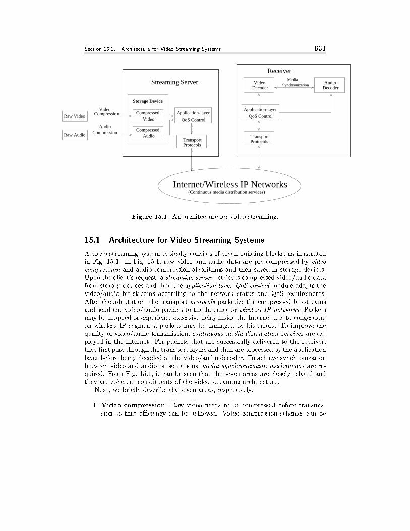
Section 15.1. Architecture for Video Streaming Systems 551
Application-layer
QoS Control
VideoDecoder
Application-layer
QoS Control
Protocols
DecoderAudioSynchronization
Media
Receiver
TransportCompression
Audio
Raw Video
Raw Audio
ProtocolsTransport
Storage Device
Compressed
Compressed
Video
Audio
Streaming Server
CompressionVideo
(Continuous media distribution services)Internet/Wireless IP Networks
Figure 15.1. An architecture for video streaming.
15.1 Architecture for Video Streaming Systems
A video streaming system typically consists of seven building blocks, as illustrated
in Fig. 15.1. In Fig. 15.1, raw video and audio data are pre-compressed by video
compression and audio compression algorithms and then saved in storage devices.
Upon the client's request, a streaming server retrieves compressed video/audio data
from storage devices and then the application-layer QoS control module adapts the
video/audio bit-streams according to the network status and QoS requirements.
After the adaptation, the transport protocols packetize the compressed bit-streams
and send the video/audio packets to the Internet or wireless IP networks. Packets
may be dropped or experience excessive delay inside the Internet due to congestion;
on wireless IP segments, packets may be damaged by bit errors. To improve the
quality of video/audio transmission, continuous media distribution services are de-
ployed in the Internet. For packets that are successfully delivered to the receiver,
they �rst pass through the transport layers and then are processed by the application
layer before being decoded at the video/audio decoder. To achieve synchronization
between video and audio presentations, media synchronization mechanisms are re-
quired. From Fig. 15.1, it can be seen that the seven areas are closely related and
they are coherent constituents of the video streaming architecture.
Next, we brie y describe the seven areas, respectively.
1. Video compression: Raw video needs to be compressed before transmis-
sion so that eÆciency can be achieved. Video compression schemes can be
552 Streaming Video over the Internet and Wireless IP Networks Chapter 15
classi�ed into two categories: scalable and non-scalable video coding. Since
scalable video is capable of gracefully coping with the bandwidth uctuations
in the Internet [45], we are primarily concerned with scalable video coding
techniques. We have covered this topic previously in Chap. 11, and thus will
only provide a brief review of this topic here.
2. Application-layer QoS control for streaming video: To cope with
changing network conditions and changing presentation quality requested by
the users, various application-layer QoS control techniques have been proposed
[19, 69, 77]. The application-layer techniques include congestion control and
error control. Their respective functions are as follows. Congestion control
is employed to prevent packet loss and reduce delay. Error control, on the
other hand, is to improve video presentation quality in presence of packet
loss. Techniques for error control for general video communication applica-
tions have been described in Chapter 14. Here, we will focus on those that
are e�ective for video streaming applications.
3. Continuous media distribution services: In order to provide quality mul-
timedia presentations, the support from the network is important. This is
because network support can reduce transport delay and packet loss ratio.
Built on top of the Internet (IP protocol), continuous media distribution ser-
vices are able to achieve QoS and eÆciency for streaming video/audio over the
best-e�ort Internet. Continuous media distribution services include network
�ltering, application-level multicast, and content replication.
4. Streaming servers: Streaming servers play a key role in providing streaming
services. To o�er quality streaming services, streaming servers are required
to process multimedia data under timing constraints and support interactive
control operations such as pause/resume, fast forward and fast backward.
Furthermore, streaming servers need to retrieve media components in a syn-
chronous fashion. A streaming server typically consists of three subsystems,
namely, a communicator (e.g., transport protocols), a operating system, and
a storage system.
5. Media synchronization mechanisms: Media synchronization is a major
feature that distinguishes multimedia applications from other traditional data
applications. With media synchronization mechanisms, the application at
the receiver side can present various media streams in the same way as they
were originally captured. An example of media synchronization is that the
movements of the lips of a speaker correspond to the presented audio.
6. Protocols for streaming media: Protocols are designed and standard-
ized for communication between clients and streaming servers. Protocols for
streaming media provide such services as network addressing, transport, and
session control. According to their functionalities, the protocols can be classi-
�ed in three categories: (1) network-layer protocol such as Internet Protocol
Section 15.2. Video Compression 553
(IP), (2) transport protocol such as User Datagram Protocol (UDP), and (3)
session control protocol such as Real-Time Streaming Protocol (RTSP).
7. Streaming video over wireless IP networks: Fluctuations of wireless
channel conditions pose many challenges to provide QoS for video transmis-
sion over wireless IP networks. To address this problem, an adaptive frame-
work has been proposed [85]. The adaptive framework includes: (1) scalable
video representations, (2) network-aware video applications, and (3) adaptive
services.
The remainder of this chapter is organized as follows. Section 15.2 discusses
video compression techniques. In Section 15.3, we present application-layer QoS
control mechanisms for streaming video. Section 15.4 describes continuous media
distribution services. In Section 15.5, we discuss key issues on design of streaming
servers. Section 15.6 presents various media synchronization mechanisms. In Sec-
tion 15.7, we overview the key protocols for streaming video. Section 15.8 presents
an adaptive framework for streaming video over wireless IP networks. Finally, a
summary is given in Section 15.9.
15.2 Video Compression
Since raw video consumes large amount of bandwidth, raw video needs to be com-
pressed before transmission so that eÆciency can be achieved. Video compression
schemes can be classi�ed into two categories: scalable and non-scalable video coding.
As described in Chap. 11, a scalable video coding scheme produces a compressed
bit-stream, parts of which are decodable. Compared with decoding the complete
bit-stream, decoding part of the compressed bit-stream produces pictures with de-
graded quality, or smaller image size, or smaller frame rate. It has been shown that
scalable video is capable of gracefully coping with the bandwidth uctuations in the
Internet [40, 45]. In contrast, non-scalable video is more susceptible to bandwidth
variations since it cannot adapt its video representation to bandwidth uctuations
[45]. Furthermore, scalable video representation is an e�ective means to achieve
eÆciency and exibility for multicasting video over heterogeneous networks (e.g.,
networks with di�erent access link bandwidth) [40, 45]. For these reasons, all the
streaming video services employ scalable video coding techniques. For a more de-
tailed discussion on various scalable coding methods, see Chap. 11. Next, we present
the application-layer QoS control mechanisms, which adapt the video bit-streams
according to the network status and QoS requirements.
15.3 Application-layer QoS Control for Streaming Video
Application-layer QoS Control is to maximize video quality in the presence of packet
loss and the changes in available bandwidth. The application-layer QoS control tech-
niques include congestion control and error control. These techniques are employed
by the end systems and do not require the QoS support from the routers/networks.
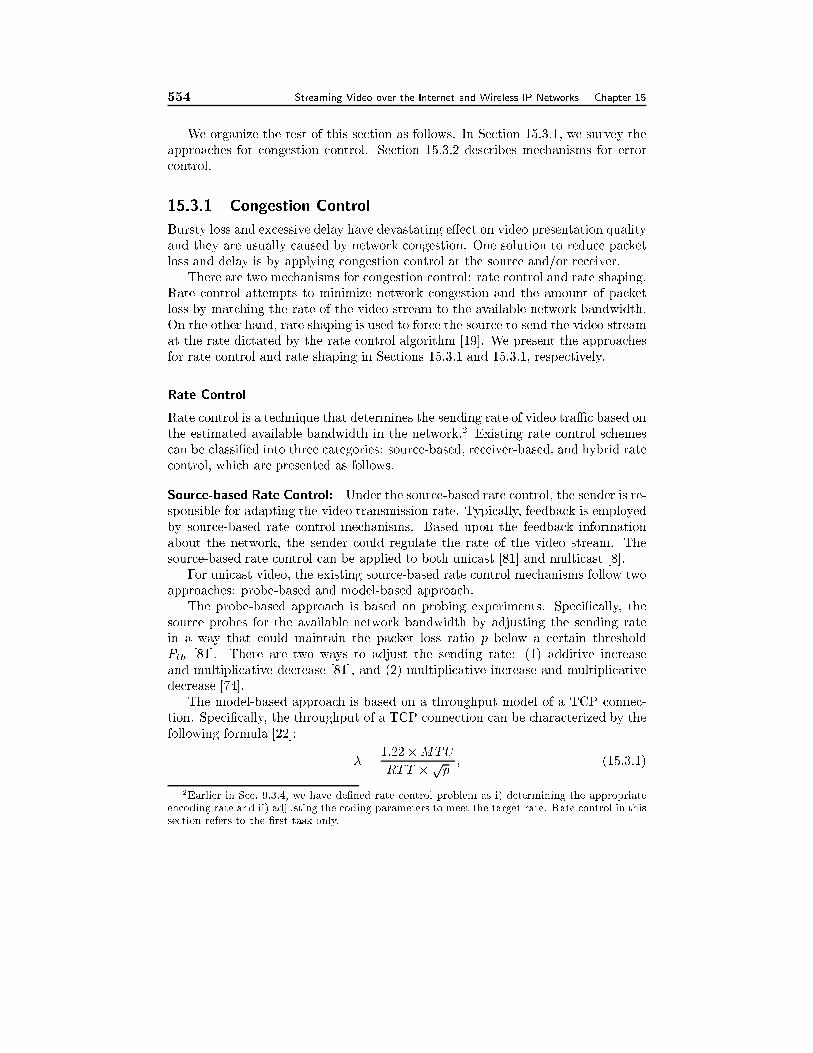
554 Streaming Video over the Internet and Wireless IP Networks Chapter 15
We organize the rest of this section as follows. In Section 15.3.1, we survey the
approaches for congestion control. Section 15.3.2 describes mechanisms for error
control.
15.3.1 Congestion Control
Bursty loss and excessive delay have devastating e�ect on video presentation quality
and they are usually caused by network congestion. One solution to reduce packet
loss and delay is by applying congestion control at the source and/or receiver.
There are two mechanisms for congestion control: rate control and rate shaping.
Rate control attempts to minimize network congestion and the amount of packet
loss by matching the rate of the video stream to the available network bandwidth.
On the other hand, rate shaping is used to force the source to send the video stream
at the rate dictated by the rate control algorithm [19]. We present the approaches
for rate control and rate shaping in Sections 15.3.1 and 15.3.1, respectively.
Rate Control
Rate control is a technique that determines the sending rate of video traÆc based on
the estimated available bandwidth in the network.2 Existing rate control schemes
can be classi�ed into three categories: source-based, receiver-based, and hybrid rate
control, which are presented as follows.
Source-based Rate Control: Under the source-based rate control, the sender is re-
sponsible for adapting the video transmission rate. Typically, feedback is employed
by source-based rate control mechanisms. Based upon the feedback information
about the network, the sender could regulate the rate of the video stream. The
source-based rate control can be applied to both unicast [81] and multicast [8].
For unicast video, the existing source-based rate control mechanisms follow two
approaches: probe-based and model-based approach.
The probe-based approach is based on probing experiments. Speci�cally, the
source probes for the available network bandwidth by adjusting the sending rate
in a way that could maintain the packet loss ratio p below a certain threshold
Pth [81]. There are two ways to adjust the sending rate: (1) additive increase
and multiplicative decrease [81], and (2) multiplicative increase and multiplicative
decrease [74].
The model-based approach is based on a throughput model of a TCP connec-
tion. Speci�cally, the throughput of a TCP connection can be characterized by the
following formula [22]:
� =1:22�MTU
RTT �pp ; (15.3.1)
2Earlier in Sec. 9.3.4, we have de�ned rate control problem as i) determining the appropriate
encoding rate and ii) adjusting the coding parameters to meet the target rate. Rate control in this
section refers to the �rst task only.
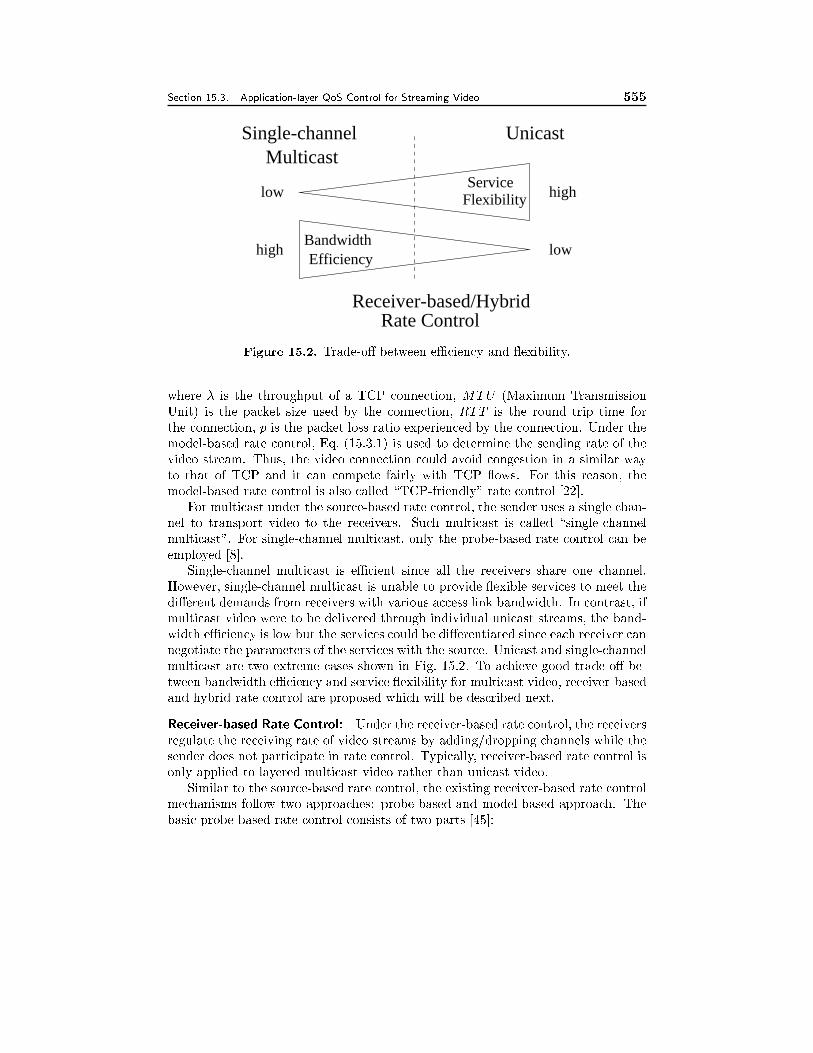
Section 15.3. Application-layer QoS Control for Streaming Video 555
Efficiencylowhigh
Bandwidth
low highFlexibilityService
Unicast
Receiver-based/HybridRate Control
Single-channelMulticast
Figure 15.2. Trade-o� between eÆciency and exibility.
where � is the throughput of a TCP connection, MTU (Maximum Transmission
Unit) is the packet size used by the connection, RTT is the round trip time for
the connection, p is the packet loss ratio experienced by the connection. Under the
model-based rate control, Eq. (15.3.1) is used to determine the sending rate of the
video stream. Thus, the video connection could avoid congestion in a similar way
to that of TCP and it can compete fairly with TCP ows. For this reason, the
model-based rate control is also called \TCP-friendly" rate control [22].
For multicast under the source-based rate control, the sender uses a single chan-
nel to transport video to the receivers. Such multicast is called \single-channel
multicast". For single-channel multicast, only the probe-based rate control can be
employed [8].
Single-channel multicast is eÆcient since all the receivers share one channel.
However, single-channel multicast is unable to provide exible services to meet the
di�erent demands from receivers with various access link bandwidth. In contrast, if
multicast video were to be delivered through individual unicast streams, the band-
width eÆciency is low but the services could be di�erentiated since each receiver can
negotiate the parameters of the services with the source. Unicast and single-channel
multicast are two extreme cases shown in Fig. 15.2. To achieve good trade-o� be-
tween bandwidth eÆciency and service exibility for multicast video, receiver-based
and hybrid rate control are proposed which will be described next.
Receiver-based Rate Control: Under the receiver-based rate control, the receivers
regulate the receiving rate of video streams by adding/dropping channels while the
sender does not participate in rate control. Typically, receiver-based rate control is
only applied to layered multicast video rather than unicast video.
Similar to the source-based rate control, the existing receiver-based rate control
mechanisms follow two approaches: probe-based and model-based approach. The
basic probe-based rate control consists of two parts [45]:
556 Streaming Video over the Internet and Wireless IP Networks Chapter 15
1. When no congestion is detected, a receiver probes for the available bandwidth
by joining a layer, resulting in increase of its receiving rate. If no congestion
is detected after the joining, the join-experiment is successful. Otherwise, the
receiver drops the newly added layer.
2. When congestion is detected, a receiver drops a layer, resulting in reduction
of its receiving rate.
Unlike the probe-based approach which implicitly estimates the available net-
work bandwidth through probing experiments, the model-based approach uses ex-
plicit estimation for the available network bandwidth. The model-based approach
is based on the throughput model of a TCP connection (i.e., Eq. 15.3.1), which is
described in the source-based rate control. Thus, the model-based rate control is
also \TCP-friendly".
Hybrid Rate Control: Under the hybrid rate control, the receivers regulate the
receiving rate of video streams by adding/dropping channels while the sender also
adjusts the transmission rate of each channel based on feedback from the receivers.
An example is Destination Set Grouping [13].
Rate Shaping
Rate shaping is a technique, through which the rate of pre-compressed video bit-
streams can be adapted to the target rate constraint. A rate shaper is an interface
(or �lter) between the compression layer and the network transport layer or between
two network segments, with which the video stream can be matched to the available
network bandwidth.
There are many types of rate shapers or �lters, which include [87]:
1. Codec �lter: A codec �lter is to decompress and compress a video stream.
It is commonly used to perform transcoding between di�erent compression
schemes. Depending on the compression scheme used, transcoding could be
simpli�ed without full decompression and recompression.
2. Frame-dropping �lter: The frame-dropping �lter can distinguish the frame
types (e.g., I-, P-, and B-frame in MPEG) and drop frames according to
importance. For example, the dropping order would be �rst B-frames, then
P-frames, and �nally I-frames. The frame-dropping �lter is used to reduce the
data rate of a video stream by discarding a number of frames and transmitting
the remaining frames at a lower rate. The frame-dropping �lter could be used
at the source [90] or used in the network (see Section 15.4.1).
3. Layer-dropping �lter: The layer-dropping �lter can distinguish the layers
and drop layers according to importance. The dropping order is from the
highest enhancement layer down to the base layer.
4. Frequency �lter: A frequency �lter performs operations on the compression
layer. Speci�cally, it operates in the frequency domain (i.e., DCT coeÆcients).
Section 15.3. Application-layer QoS Control for Streaming Video 557
Frequency �ltering mechanisms include low-pass �ltering, color reduction �l-
tering and color-to-monochrome �ltering.
Low-pass �ltering is to discard the DCT coeÆcients of the higher frequencies.
A color reduction �lter performs the same operation as a low-pass �lter except
that it only operates on the chrominance information in the video stream.
A color-to-monochrome �lter removes all color information from the video
stream. In MPEG, this is done by replacing each chrominance block by an
empty block.
Unlike the frame-dropping �lter, the frequency �lter reduces the bandwidth
without a�ecting the frame rate. Its cost is reduction in presentation quality
of the resulting frame.
5. Re-quantization �lter: The re-quantization �lter performs operations on
the compression layer (i.e., DCT coeÆcients). The �lter �rst extracts the DCT
coeÆcients from the compressed video stream through dequantization. Then
the �lter re-quantizes the DCT coeÆcients with a larger quantizer stepsize,
resulting in rate reduction.
As a summary, the purpose of congestion control is to prevent packet loss. The
fact that packet loss is inevitable in the Internet and may have signi�cant impact
on perceptual quality prompts the need to design mechanisms to maximize video
presentation quality in presence of packet loss. Error control is such a mechanism,
which will be presented next.
15.3.2 Error Control
Techniques for error control in video communication have been discussed in Chap. 14.
There, we have classi�ed error control techniques into four categories: transport
level error control, including FEC and delay-constrained retransmission, encoder
error-resilient coding, decoder error concealment, and encoder and decoder interac-
tive error control. Here, we describe several techniques that are e�ective for video
streaming applications.
FEC
The principle of FEC is to add redundant information so that original message can
be reconstructed in presence of packet loss. For Internet applications, block codes
are typically used for channel coding. Speci�cally, a video stream is �rst chopped
into segments, each of which is packetized into k packets; then for each segment, a
block code (e.g., Tornado code [1]) is applied to the k packets to generate a n-packet
block, where n > k. To perfectly recover a segment, a user only needs to receive
any k packets in the n-packet block.
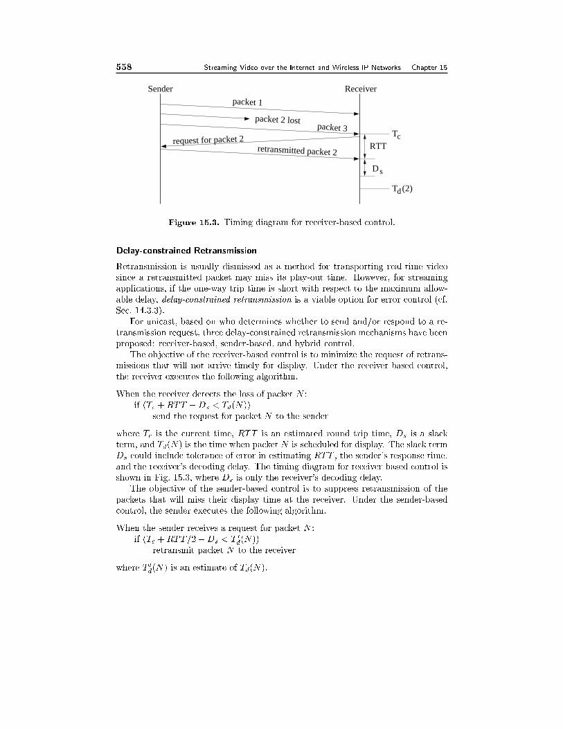
558 Streaming Video over the Internet and Wireless IP Networks Chapter 15
RTTTc
Sender Receiver
request for packet 2retransmitted packet 2
packet 1
packet 2 lostpacket 3
T (2)d
Ds
Figure 15.3. Timing diagram for receiver-based control.
Delay-constrained Retransmission
Retransmission is usually dismissed as a method for transporting real-time video
since a retransmitted packet may miss its play-out time. However, for streaming
applications, if the one-way trip time is short with respect to the maximum allow-
able delay, delay-constrained retransmission is a viable option for error control (cf.
Sec. 14.3.3).
For unicast, based on who determines whether to send and/or respond to a re-
transmission request, three delay-constrained retransmission mechanisms have been
proposed: receiver-based, sender-based, and hybrid control.
The objective of the receiver-based control is to minimize the request of retrans-
missions that will not arrive timely for display. Under the receiver-based control,
the receiver executes the following algorithm.
When the receiver detects the loss of packet N :
if (Tc +RTT +Ds < Td(N))
send the request for packet N to the sender
where Tc is the current time, RTT is an estimated round trip time, Ds is a slack
term, and Td(N) is the time when packet N is scheduled for display. The slack term
Ds could include tolerance of error in estimating RTT , the sender's response time,
and the receiver's decoding delay. The timing diagram for receiver-based control is
shown in Fig. 15.3, where Ds is only the receiver's decoding delay.
The objective of the sender-based control is to suppress retransmission of the
packets that will miss their display time at the receiver. Under the sender-based
control, the sender executes the following algorithm.
When the sender receives a request for packet N :
if (Tc +RTT=2+Ds < T0
d(N))
retransmit packet N to the receiver
where T 0
d(N) is an estimate of Td(N).
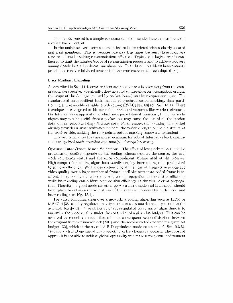
Section 15.3. Application-layer QoS Control for Streaming Video 559
The hybrid control is a simple combination of the sender-based control and the
receiver-based control.
In the multicast case, retransmission has to be restricted within closely located
multicast members. This is because one-way trip times between these members
tend to be small, making retransmissions e�ective. Typically, a logical tree is con-
�gured to limit the number/scope of retransmission requests and to achieve recovery
among closely located multicast members [86]. In addition, to address heterogeneity
problem, a receiver-initiated mechanism for error recovery can be adopted [86].
Error Resilient Encoding
As described in Sec. 14.4, error-resilient schemes address loss recovery from the com-
pression perspective. Speci�cally, they attempt to prevent error propagation or limit
the scope of the damage (caused by packet losses) on the compression layer. The
standardized error-resilient tools include re-synchronization marking, data parti-
tioning, and reversible variable length coding (RVLC) [35, 68] (cf. Sec. 14.4). These
techniques are targeted at bit-error dominant environments like wireless channels.
For Internet video applications, which uses packet-based transport, the above tech-
niques may not be useful since a packet loss may cause the loss of all the motion
data and its associated shape/texture data. Furthermore, the boundary of a packet
already provides a synchronization point in the variable-length coded bit-stream at
the receiver side, making the re-synchronization marking somewhat redundant.
The two techniques that are more promising for robust Internet video transmis-
sion are optimal mode selection and multiple description coding.
Optimal Intra/Inter Mode Selection: The e�ect of lost packets on the video
presentation quality depends on the coding scheme used at the source, the net-
work congestion status and the error concealment scheme used at the receiver.
High-compression coding algorithms usually employ inter-coding (i.e., prediction)
to achieve eÆciency. With these coding algorithms, loss of a packet may degrade
video quality over a large number of frames, until the next intra-coded frame is re-
ceived. Intra-coding can e�ectively stop error propagation at the cost of eÆciency
while inter-coding can achieve compression eÆciency at the risk of error propaga-
tion. Therefore, a good mode selection between intra mode and inter mode should
be in place to enhance the robustness of the video compressed by both intra- and
inter-coding (see Fig. 15.4).
For video communication over a network, a coding algorithm such as H.263 or
MPEG-4 [35] usually regulates its output rate so as to match the output rate to the
available bandwidth. The objective of rate-regulated compression algorithms is to
maximize the video quality under the constraint of a given bit budget. This can be
achieved by choosing a mode that minimizes the quantization distortion between
the original frame or macroblock (MB) and the reconstructed one under a given bit
budget [52], which is the so-called R-D optimized mode selection (cf. Sec. 9.3.3).
We refer such R-D optimized mode selection as the classical approach. The classical
approach is not able to achieve global optimality under the error-prone environment
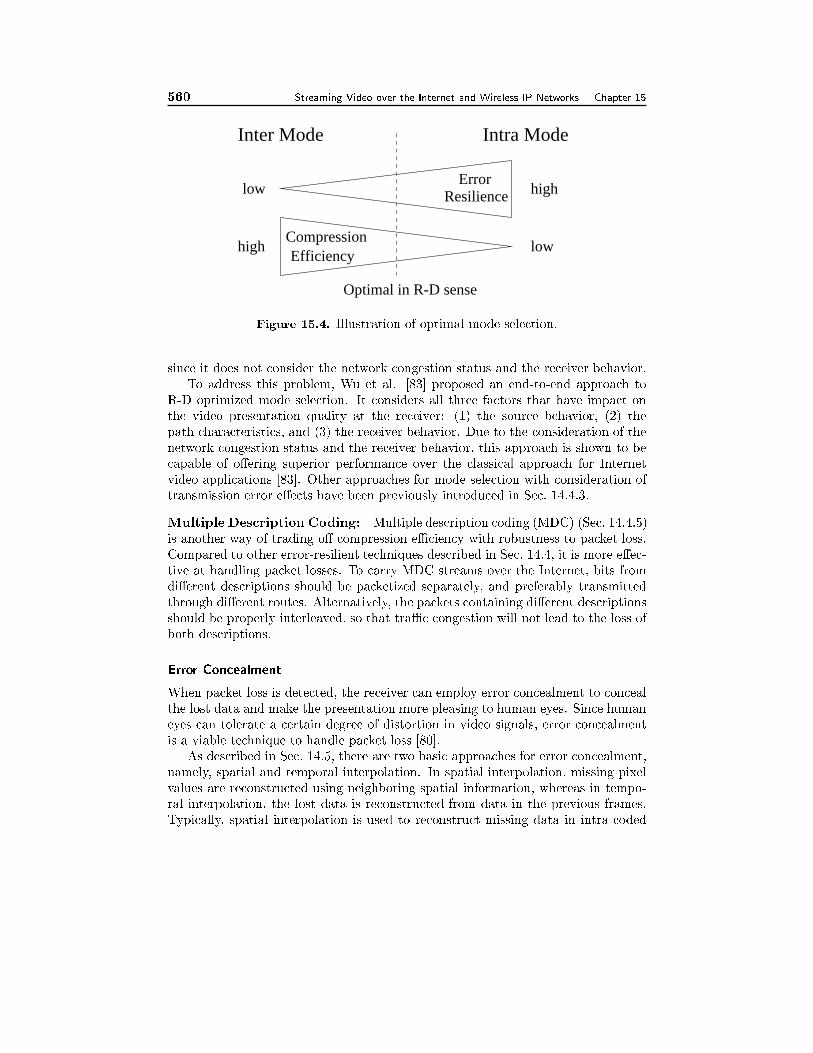
560 Streaming Video over the Internet and Wireless IP Networks Chapter 15
ResilienceError
low high
Inter Mode Intra Mode
CompressionEfficiency
lowhigh
Optimal in R-D sense
Figure 15.4. Illustration of optimal mode selection.
since it does not consider the network congestion status and the receiver behavior.
To address this problem, Wu et al. [83] proposed an end-to-end approach to
R-D optimized mode selection. It considers all three factors that have impact on
the video presentation quality at the receiver: (1) the source behavior, (2) the
path characteristics, and (3) the receiver behavior. Due to the consideration of the
network congestion status and the receiver behavior, this approach is shown to be
capable of o�ering superior performance over the classical approach for Internet
video applications [83]. Other approaches for mode selection with consideration of
transmission error e�ects have been previously introduced in Sec. 14.4.3.
Multiple Description Coding: Multiple description coding (MDC) (Sec. 14.4.5)
is another way of trading o� compression eÆciency with robustness to packet loss.
Compared to other error-resilient techniques described in Sec. 14.4, it is more e�ec-
tive at handling packet losses. To carry MDC streams over the Internet, bits from
di�erent descriptions should be packetized separately, and preferably transmitted
through di�erent routes. Alternatively, the packets containing di�erent descriptions
should be properly interleaved, so that traÆc congestion will not lead to the loss of
both descriptions.
Error Concealment
When packet loss is detected, the receiver can employ error concealment to conceal
the lost data and make the presentation more pleasing to human eyes. Since human
eyes can tolerate a certain degree of distortion in video signals, error concealment
is a viable technique to handle packet loss [80].
As described in Sec. 14.5, there are two basic approaches for error concealment,
namely, spatial and temporal interpolation. In spatial interpolation, missing pixel
values are reconstructed using neighboring spatial information, whereas in tempo-
ral interpolation, the lost data is reconstructed from data in the previous frames.
Typically, spatial interpolation is used to reconstruct missing data in intra-coded
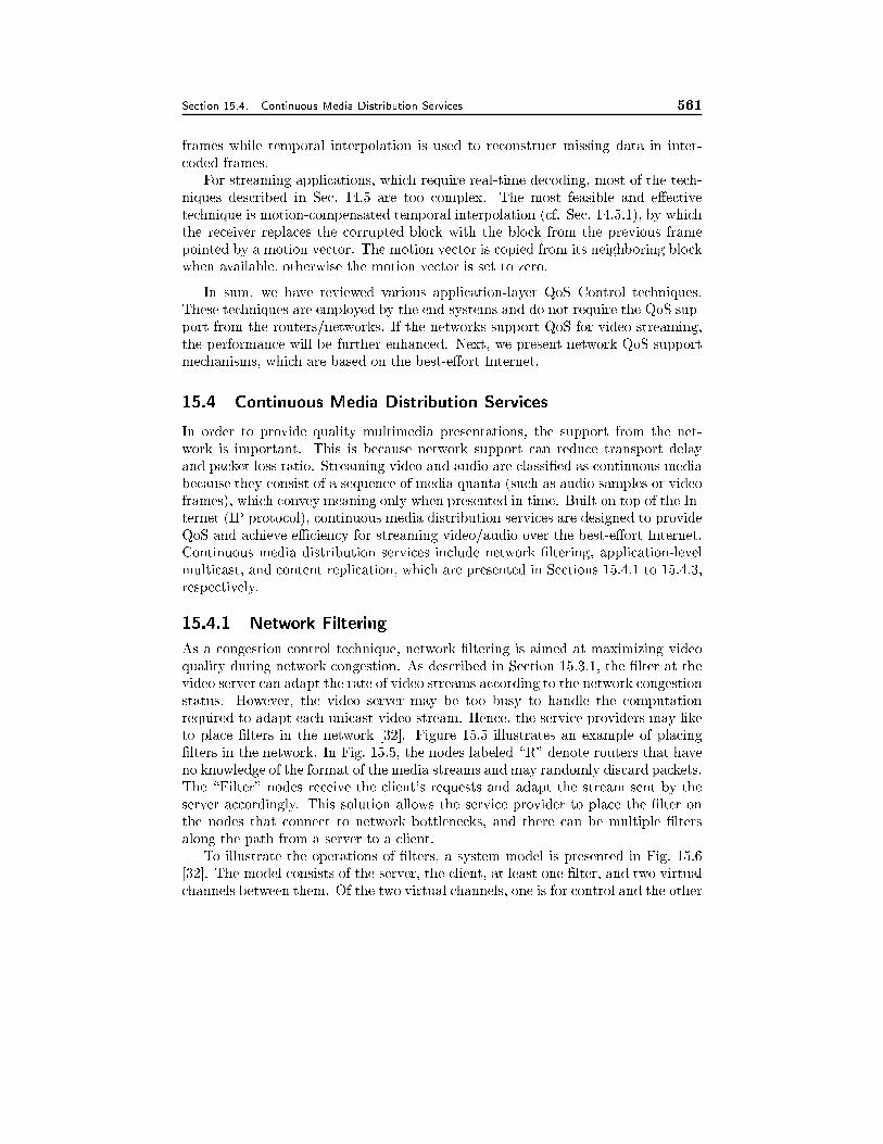
Section 15.4. Continuous Media Distribution Services 561
frames while temporal interpolation is used to reconstruct missing data in inter-
coded frames.
For streaming applications, which require real-time decoding, most of the tech-
niques described in Sec. 14.5 are too complex. The most feasible and e�ective
technique is motion-compensated temporal interpolation (cf. Sec. 14.5.1), by which
the receiver replaces the corrupted block with the block from the previous frame
pointed by a motion vector. The motion vector is copied from its neighboring block
when available, otherwise the motion vector is set to zero.
In sum, we have reviewed various application-layer QoS Control techniques.
These techniques are employed by the end systems and do not require the QoS sup-
port from the routers/networks. If the networks support QoS for video streaming,
the performance will be further enhanced. Next, we present network QoS support
mechanisms, which are based on the best-e�ort Internet.
15.4 Continuous Media Distribution Services
In order to provide quality multimedia presentations, the support from the net-
work is important. This is because network support can reduce transport delay
and packet loss ratio. Streaming video and audio are classi�ed as continuous media
because they consist of a sequence of media quanta (such as audio samples or video
frames), which convey meaning only when presented in time. Built on top of the In-
ternet (IP protocol), continuous media distribution services are designed to provide
QoS and achieve eÆciency for streaming video/audio over the best-e�ort Internet.
Continuous media distribution services include network �ltering, application-level
multicast, and content replication, which are presented in Sections 15.4.1 to 15.4.3,
respectively.
15.4.1 Network Filtering
As a congestion control technique, network �ltering is aimed at maximizing video
quality during network congestion. As described in Section 15.3.1, the �lter at the
video server can adapt the rate of video streams according to the network congestion
status. However, the video server may be too busy to handle the computation
required to adapt each unicast video stream. Hence, the service providers may like
to place �lters in the network [32]. Figure 15.5 illustrates an example of placing
�lters in the network. In Fig. 15.5, the nodes labeled \R" denote routers that have
no knowledge of the format of the media streams and may randomly discard packets.
The \Filter" nodes receive the client's requests and adapt the stream sent by the
server accordingly. This solution allows the service provider to place the �lter on
the nodes that connect to network bottlenecks, and there can be multiple �lters
along the path from a server to a client.
To illustrate the operations of �lters, a system model is presented in Fig. 15.6
[32]. The model consists of the server, the client, at least one �lter, and two virtual
channels between them. Of the two virtual channels, one is for control and the other
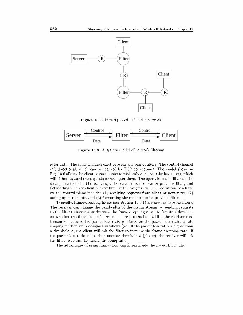
562 Streaming Video over the Internet and Wireless IP Networks Chapter 15
Server R Filter
R R
Client
Filter
R
Client
Client
Figure 15.5. Filters placed inside the network.
Server Filter ClientControl Control
Data Data
Figure 15.6. A system model of network �ltering.
is for data. The same channels exist between any pair of �lters. The control channel
is bidirectional, which can be realized by TCP connections. The model shown in
Fig. 15.6 allows the client to communicate with only one host (the last �lter), which
will either forward the requests or act upon them. The operations of a �lter on the
data plane include: (1) receiving video stream from server or previous �lter, and
(2) sending video to client or next �lter at the target rate. The operations of a �lter
on the control plane include: (1) receiving requests from client or next �lter, (2)
acting upon requests, and (3) forwarding the requests to its previous �lter.
Typically, frame-dropping �lters (see Section 15.3.1) are used as network �lters.
The receiver can change the bandwidth of the media stream by sending requests
to the �lter to increase or decrease the frame dropping rate. To facilitate decisions
on whether the �lter should increase or decrease the bandwidth, the receiver con-
tinuously measures the packet loss ratio p. Based on the packet loss ratio, a rate
shaping mechanism is designed as follows [32]. If the packet loss ratio is higher than
a threshold �, the client will ask the �lter to increase the frame dropping rate. If
the packet loss ratio is less than another threshold � (� < �), the receiver will ask
the �lter to reduce the frame dropping rate.
The advantages of using frame-dropping �lters inside the network include:
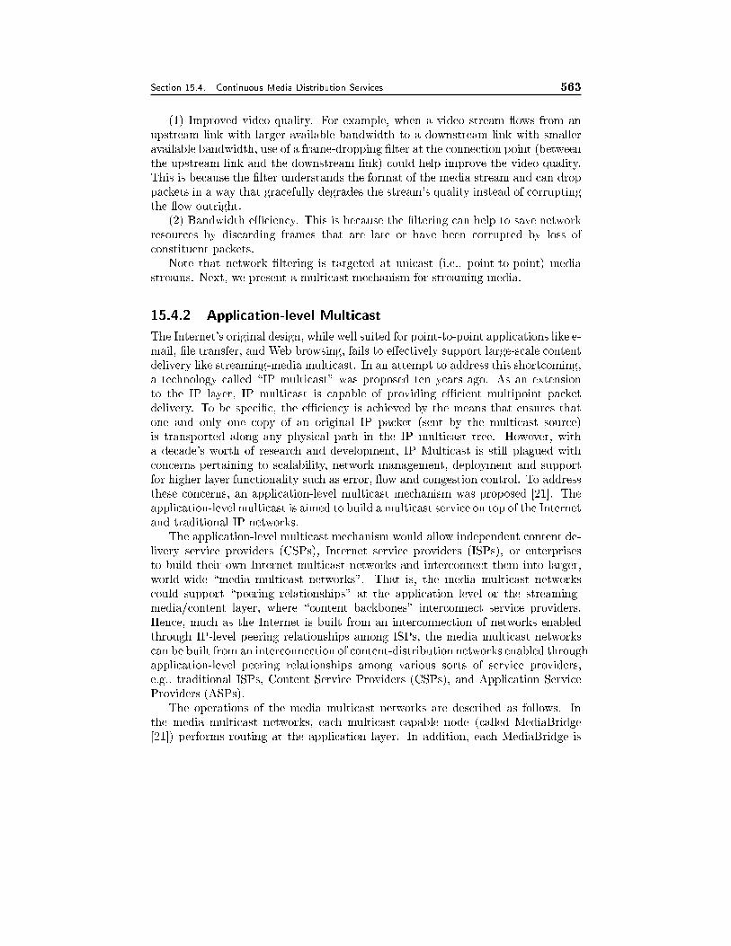
Section 15.4. Continuous Media Distribution Services 563
(1) Improved video quality. For example, when a video stream ows from an
upstream link with larger available bandwidth to a downstream link with smaller
available bandwidth, use of a frame-dropping �lter at the connection point (between
the upstream link and the downstream link) could help improve the video quality.
This is because the �lter understands the format of the media stream and can drop
packets in a way that gracefully degrades the stream's quality instead of corrupting
the ow outright.
(2) Bandwidth eÆciency. This is because the �ltering can help to save network
resources by discarding frames that are late or have been corrupted by loss of
constituent packets.
Note that network �ltering is targeted at unicast (i.e., point-to-point) media
streams. Next, we present a multicast mechanism for streaming media.
15.4.2 Application-level Multicast
The Internet's original design, while well suited for point-to-point applications like e-
mail, �le transfer, and Web browsing, fails to e�ectively support large-scale content
delivery like streaming-media multicast. In an attempt to address this shortcoming,
a technology called \IP multicast" was proposed ten years ago. As an extension
to the IP layer, IP multicast is capable of providing eÆcient multipoint packet
delivery. To be speci�c, the eÆciency is achieved by the means that ensures that
one and only one copy of an original IP packet (sent by the multicast source)
is transported along any physical path in the IP multicast tree. However, with
a decade's worth of research and development, IP Multicast is still plagued with
concerns pertaining to scalability, network management, deployment and support
for higher layer functionality such as error, ow and congestion control. To address
these concerns, an application-level multicast mechanism was proposed [21]. The
application-level multicast is aimed to build a multicast service on top of the Internet
and traditional IP networks.
The application-level multicast mechanism would allow independent content de-
livery service providers (CSPs), Internet service providers (ISPs), or enterprises
to build their own Internet multicast networks and interconnect them into larger,
world-wide \media multicast networks". That is, the media multicast networks
could support \peering relationships" at the application level or the streaming-
media/content layer, where \content backbones" interconnect service providers.
Hence, much as the Internet is built from an interconnection of networks enabled
through IP-level peering relationships among ISPs, the media multicast networks
can be built from an interconnection of content-distribution networks enabled through
application-level peering relationships among various sorts of service providers,
e.g., traditional ISPs, Content Service Providers (CSPs), and Application Service
Providers (ASPs).
The operations of the media multicast networks are described as follows. In
the media multicast networks, each multicast-capable node (called MediaBridge
[21]) performs routing at the application layer. In addition, each MediaBridge is
564 Streaming Video over the Internet and Wireless IP Networks Chapter 15
interconnected with one or more neighboring MediaBridge through explicit con-
�guration, which de�nes the application-level overlay topology. Collectively, the
MediaBridges in a media multicast network employ a distributed application-level
multicast routing algorithm to determine the optimal virtual paths for propagating
content throughout the network. When the underlying network fails or becomes
overly congested, the media multicast network automatically and dynamically re-
routes content via alternate paths according to application-level routing policies. In
addition, MediaBridges dynamically subscribe to multicast content when and only
when a downstream client requests it. This capability ensures that one and only one
copy of the multicast content ows across any physical or virtual path independent
of the number of downstream clients, resulting in conserving network bandwidth.
The advantage of the application-level multicast is that it breaks the barriers
such as scalability, network management, support for congestion control, which have
prevented ISPs from establishing \IP multicast" peering arrangements.
15.4.3 Content Replication
A fundamental technique for improving scalability of the media delivery system
is content/media replication. The content replication takes two forms, namely,
caching and mirroring, which are deployed by publisher, Content Service Providers
and ISPs. Both caching and mirroring seek to place content closer to the clients
and both share the following advantages:
1. reduced bandwidth consumption on network links,
2. reduced load on streaming servers,
3. reduced latency for clients,
4. increased availability.
Mirroring is to place copies of the original multimedia �les on several machines
scattered around the Internet. That is, the original multimedia �les are stored
on the main server while copies of the original multimedia �les are placed on the
duplicate servers. In this way, clients can retrieve multimedia data from the nearest
duplicate server, which gives the clients the best performance (e.g., lowest latency).
Mirroring has several advantages as follows:
� all contents are replicated;
� the publisher is able to view server access logs and perform user tracking.
On the other hand, there are a number of disadvantages with mirroring. Cur-
rently, mechanisms for establishing dedicated mirrors are expensive, ad hoc, and
slow. In addition, establishing a mirror on an existing server, while cheaper, is still
an ad hoc and administratively complex process. Finally, there is no standard way
to make scripts and server setup easily transferable from one server to another.
Section 15.5. Streaming Servers 565
Caching, which is based on the belief that di�erent clients will load many of the
same contents, makes local copies of contents that the clients retrieve. Typically,
clients in a single organization retrieve all contents from a single local machine,
called a cache. The cache retrieves a video �le from the streaming server, storing
a copy locally and then passing it on to the client who requests it. If a client asks
for a video �le which the cache has already stored, the cache will return the copy
rather than going all the way back to the streaming server on which the video �le
resides. In addition, cache sharing and cache hierarchies allow each cache to access
�les stored at other caches so that the load on the main server can be reduced and
network bottlenecks can be alleviated [11, 20].
Caching has the following advantages:
� caches can form a shared infrastructure which works for all streaming servers;
� caches are incrementally deployable.
For these reasons, ISPs have been the largest proponent of caching. However,
caches cannot supply the services that publishers need: support for quality of service
and security. Firstly, when a cache stores a publisher's document, it makes no
promises about how well the document will be treated. The publisher has no way
of requesting that its document be delivered within certain time bounds, or that
the cache verify the freshness of its copy of the document. Secondly, today's caches
trust everyone, so attacks such as inserting fake versions of documents into the
cache are extremely easy to accomplish. Finally, caches do not provide feedback to
publishers so that publishers are unable to perform user tracking.
Most of the techniques on caching are targeted at generic web objects. Some re-
cent work demonstrated that caching strategies that are speci�c of particular types
of objects can help improve the overall performance [46]. For this reason, a great
deal of e�orts have been contributed along this direction [46, 58, 62, 91]. A trivial
extension of caching techniques to video is to store complete video sequences in the
cache. However, such an approach may not be applicable due to the large scale of
video data size and possibly limited cache space on a proxy server. Instead, it was
shown that only a few cached frames can also contribute to signi�cant improvement
in performance [46]. Miao and Ortega proposed two video caching strategies, initial
caching and selective caching, which store part of the video stream onto the cache
[46]. In particular, it was shown that selective caching can maximize the robust-
ness of the video stream against network congestion while not violating the limited
decoder bu�er size.
In this section, we have described three network support mechanims for stream-
ing media. Next, we discuss key issues on design of streaming servers.
15.5 Streaming Servers
Streaming servers play a key role in providing streaming services. To o�er quality
streaming services, streaming servers are required to process multimedia data un-

566 Streaming Video over the Internet and Wireless IP Networks Chapter 15
der timing constraints in order to prevent artifacts (e.g., jerkiness in video motion
and pops in audio) during playback at the clients. In addition, streaming servers
also need to support VCR-like control operations such as stop, pause/resume, fast
forward and fast reverse. Furthermore, streaming servers have to retrieve media
components in a synchronous fashion. For example, retrieving a lecture presenta-
tion requires synchronizing video and audio with lecture slides.
A streaming server typically consists of the following three subsystems:
1. Communicator: A communicator involves the application layer and trans-
port protocols implemented on the server (shown in Fig. 15.1). Through a
communicator, the clients can communicate with a server and retrieve multi-
media contents in a continuous and synchronous manner. We have addressed
the application layer in Section 15.3 and will address transport protocols in
Section 15.7.
2. Operating system: Di�erent from traditional operating systems, an oper-
ating system for streaming services needs to satisfy real-time requirements for
streaming applications.
3. Storage system: A storage system for streaming services has to support
continuous media storage and retrieval.
In this section, we are primarily concerned with operating system support and
storage systems for streaming media, which will be presented in Sections 15.5.1 and
15.5.2, respectively.
15.5.1 Real-time Operating System
The operating system shields the computer hardware from all other software. The
operating system o�ers various services related to the essential resources, such as
the CPU, main memory, storage, and all input and output devices. In the following
sections, we discuss the unique issues of real-time operating systems and review the
associated approaches to the problems introduced by streaming services. We �rst
show how process management takes into account the timing requirements imposed
by streaming media and apply appropriate scheduling methods; We then describe
how to manage resources to accommodate timing requirements; Finally, we discuss
issues on �le management.
Process Management
Process management deals with the main processor resource. The process manager
maps single processes onto the CPU resource according to a speci�ed scheduling
policy such that all processes can meet their requirements.
To ful�ll the timing requirements of continuous media, the operating system
must use real-time scheduling techniques. Most attempts to solve real-time schedul-
ing problems are just variations of two basic algorithms for multimedia systems: ear-
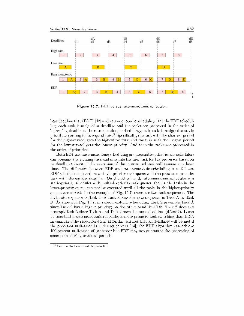
Section 15.5. Streaming Servers 567
5
1
61
3 D
2
B 5
7
C
8
7
86
3 4
51 4
6
3
4
72
A 2 8
Rate monotonic
A B C D
A A B B C C D D
EDF
Low rate
High rate
Deadlines d1 d2 d3 d4 d5 d6 d7 d8
t
dA dB dC dD
Figure 15.7. EDF versus rate-monotonic scheduler.
liest deadline �rst (EDF) [42] and rate-monotonic scheduling [14]. In EDF schedul-
ing, each task is assigned a deadline and the tasks are processed in the order of
increasing deadlines. In rate-monotonic scheduling, each task is assigned a static
priority according to its request rate.3 Speci�cally, the task with the shortest period
(or the highest rate) gets the highest priority, and the task with the longest period
(or the lowest rate) gets the lowest priority. And then the tasks are processed in
the order of priorities.
Both EDF and rate-monotonic scheduling are preemptive, that is, the schedulers
can preempt the running task and schedule the new task for the processor based on
its deadline/priority. The execution of the interrupted task will resume at a later
time. The di�erence between EDF and rate-monotonic scheduling is as follows.
EDF scheduler is based on a single priority task queue and the processor runs the
task with the earliest deadline. On the other hand, rate-monotonic scheduler is a
static-priority scheduler with multiple-priority task queues, that is, the tasks in the
lower-priority queue can not be executed until all the tasks in the higher-priority
queues are served. In the example of Fig. 15.7, there are two task sequences. The
high rate sequence is Task 1 to Task 8; the low rate sequence is Task A to Task
D. As shown in Fig. 15.7, in rate-monotonic scheduling, Task 2 preempts Task A
since Task 2 has a higher priority; on the other hand, in EDF, Task 2 does not
preempt Task A since Task A and Task 2 have the same deadlines (dA=d2). It can
be seen that a rate-monotonic scheduler is more prone to task switching than EDF.
In summary, the rate-monotonic algorithm ensures that all deadlines will be met if
the processor utilization is under 69 percent [14]; the EDF algorithm can achieve
100 percent utilization of processor but EDF may not guarantee the processing of
some tasks during overload periods.
3Assume that each task is periodic.
568 Streaming Video over the Internet and Wireless IP Networks Chapter 15
Resource Management
Resources in a multimedia server include CPUs, memories, storage devices, etc.
Since resources are limited, a multimedia server can only service a limited number of
clients with requested QoS. Therefore, resource management is required to manage
resources to accommodate timing requirements. Resource management involves
admission control and resource allocation. Speci�cally, before admitting a new
client, a multimedia server must perform admission control test to decide whether a
new connection can be admitted without violating performance guarantees already
provided to existing connections. If a connection is accepted, the resource manager
allocates resources required to meet the QoS for the new connection.
Admission control algorithms can be classi�ed into two categories: deterministic
admission control [24] and statistical admission control [76]. Deterministic admis-
sion control algorithms provide hard guarantees to clients while statistical admission
control algorithms provide statistical guarantees to clients (i.e., the continuity re-
quirements of at least a �xed percentage of media units are ensured to be met).
The advantages of deterministic admission control are simplicity and strict assur-
ance of quality; its limitation is lower utilization of server resources. In contrast
to this, statistical admission control improves the utilization of server resources by
exploiting the human perceptual tolerances as well as the di�erences between the
average and the worst-case performance characteristics of a multimedia server [76].
Corresponding to admission control algorithms, resource allocation schemes can
be either deterministic or statistical. Deterministic admission control algorithms
require deterministic resource allocation schemes while statistical admission control
algorithms require statistical resource allocation schemes. Deterministic resource
allocation schemes make reservations for the worst case, e.g., reserving bandwidth
for the longest processing time and the highest rate that a task might ever need.
On the other hand, statistical resource allocation schemes achieve higher utilization
by allowing temporary overload, resulting in a small percentage of QoS violations.
File Management
The �le system provides access and control functions for �le storage and retrieval.
There are two basic approaches to supporting continuous media in �le systems. In
the �rst approach, the organization of �les on disks remains as it is for discrete data
(i.e., a �le is not scattered across several disks), with the necessary real-time support
provided through special disk-scheduling algorithms and enough bu�er capacity to
avoid jitter. The second approach is to organize audio and video �les on distributed
storage like disk arrays. Under the second approach, the disk throughput can be
improved by scattering/striping each audio/video �le across several disks; disk seek-
times can be reduced by disk-scheduling algorithms.
Traditional disk-scheduling algorithms such as First-Come-First-Server and SCAN
[16, 70] do not provide real-time guarantees. Hence, many disk-scheduling algo-
rithms have been proposed in support of continuous media. These include SCAN-
EDF [56], Grouped Sweeping Scheduling (GSS) [88], and Dynamic Circular SCAN
Section 15.5. Streaming Servers 569
(DC-SCAN) [31], which are described as follows.
� The SCAN-EDF combines the seek optimization of the traditional disk-scheduling
method SCAN [16] and the real-time guarantees of the EDF mechanism. Note
that the EDF mechanism in disk scheduling is non-preemptive, which is dif-
ferent from the preemptive EDF scheme used in process management.
� The Grouped Sweeping Scheduling divides the set of n streams into g groups;
groups can be formed in such a way that all streams belonging to the same
group have similar deadlines; individual streams within a group are served
according to SCAN.
� DC-SCAN employs a Circular SCAN [64] service order to minimize disk seek
overhead and variations in inter-service time, resulting in high throughput; it
reduces start-up delay by dynamically adapting the Circular SCAN service
order.
As a result, the three algorithms, SCAN-EDF, GSS and DC-SCAN, can improve
continuous media data throughput and meet real-time requirements imposed by
continuous media.
Another function that needs to be supported by �le management is interactive
control such as pause/resume, fast forward and fast reverse. First, the pause/resume
operations pose a signi�cant challenge to the design of eÆcient bu�er management
schemes because they interfere with the sharing of a multimedia stream among dif-
ferent viewers. This issue is still under study. Secondly, the fast-forward and fast-
reverse operations can be implemented either by playing back media at a higher
rate than normal or by continuing playback at the normal rate while skipping some
data. Since the former approach can signi�cantly increase the data rate, its direct
implementation is impractical. The latter approach, on the other hand, needs to
be carefully designed if inter-data dependencies are present (for example, P frames
and B frames depend on I frames in MPEG) [12]. As a result, for streaming MPEG
video, entire Group of Pictures (GOPs) have to be skipped during fast-forward op-
erations, and the viewer sees normal resolution video with gaps, which is acceptable.
15.5.2 Storage System
The challenging issues of designing storage systems for multimedia are high through-
put, large capacity and fault-tolerance, which are addressed as follows.
Data striping: a method to increase throughput
If an entire video �le is stored on one disk, the number of concurrent accesses to that
�le are limited by the throughput of that disk. This dictates the number of clients
that are viewing the same video �le. To overcome this limitation, data stripping was
proposed [63]. Under data striping schemes, a multimedia �le is scattered across
multiple disks and the disk array can be accessed in parallel. An example of data
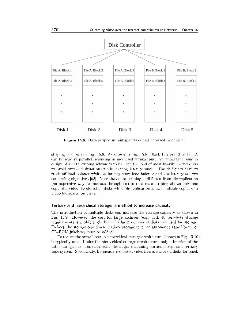
570 Streaming Video over the Internet and Wireless IP Networks Chapter 15
Disk Controller
.
.
...
...
...
...
.
Disk 1 Disk 2 Disk 3 Disk 4 Disk 5
File A, Block 1 File A, Block 2 File A, Block 3 File B, Block 1 File B, Block 2
File A, Block 4 File A, Block 5 File A, Block 6 File B, Block 3 File B, Block 4
Figure 15.8. Data striped in multiple disks and accessed in parallel.
striping is shown in Fig. 15.8. As shown in Fig. 15.8, Block 1, 2 and 3 of File A
can be read in parallel, resulting in increased throughput. An important issue in
design of a data striping scheme is to balance the load of most heavily loaded disks
to avoid overload situations while keeping latency small. The designers have to
trade o� load balance with low latency since load balance and low latency are two
con icting objectives [63]. Note that data striping is di�erent from �le replication
(an expensive way to increase throughput) in that data striping allows only one
copy of a video �le stored on disks while �le replication allows multiple copies of a
video �le stored on disks.
Tertiary and hierarchical storage: a method to increase capacity
The introduction of multiple disks can increase the storage capacity as shown in
Fig. 15.9. However, the cost for large archives (e.g., with 40 tera-byte storage
requirement) is prohibitively high if a large number of disks are used for storage.
To keep the storage cost down, tertiary storage (e.g., an automated tape library or
CD-ROM jukebox) must be added.
To reduce the overall cost, a hierarchical storage architecture (shown in Fig. 15.10)
is typically used. Under the hierarchical storage architecture, only a fraction of the
total storage is kept on disks while the major remaining portion is kept on a tertiary
tape system. Speci�cally, frequently requested video �les are kept on disks for quick
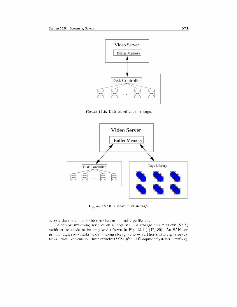
Section 15.5. Streaming Servers 571
Buffer Memory
. . .
Disk Controller
Video Server
Figure 15.9. Disk-based video storage.
Buffer Memory
Video Server
. . .
Disk Controller Tape Library
Figure 15.10. Hierarchical storage.
access; the remainder resides in the automated tape library.
To deploy streaming services on a large scale, a storage area network (SAN)
architecture needs to be employed (shown in Fig. 15.11) [17, 29]. An SAN can
provide high-speed data pipes between storage devices and hosts at far greater dis-
tances than conventional host-attached SCSI (Small Computer Systems Interface).
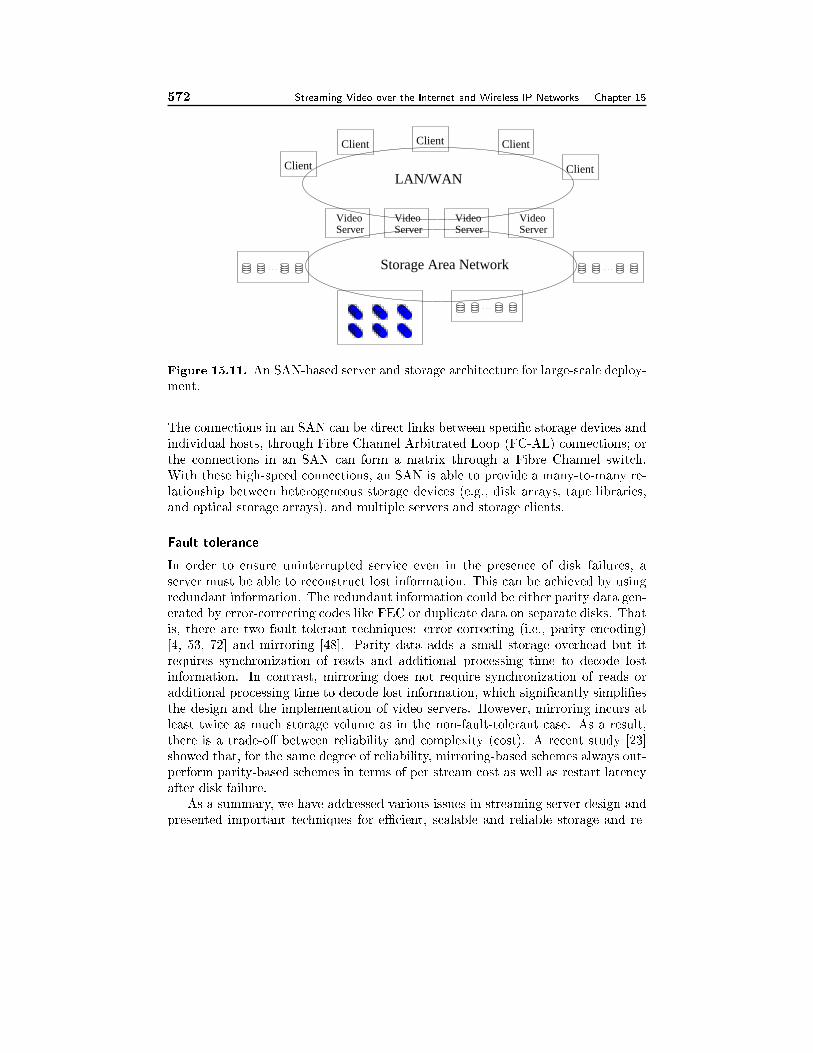
572 Streaming Video over the Internet and Wireless IP Networks Chapter 15
VideoServer
VideoServer
VideoServer
VideoServer
. . .
. . . . . .
Client
Client Client Client
Client
Storage Area Network
LAN/WAN
Figure 15.11. An SAN-based server and storage architecture for large-scale deploy-
ment.
The connections in an SAN can be direct links between speci�c storage devices and
individual hosts, through Fibre Channel Arbitrated Loop (FC-AL) connections; or
the connections in an SAN can form a matrix through a Fibre Channel switch.
With these high-speed connections, an SAN is able to provide a many-to-many re-
lationship between heterogeneous storage devices (e.g., disk arrays, tape libraries,
and optical storage arrays), and multiple servers and storage clients.
Fault tolerance
In order to ensure uninterrupted service even in the presence of disk failures, a
server must be able to reconstruct lost information. This can be achieved by using
redundant information. The redundant information could be either parity data gen-
erated by error-correcting codes like FEC or duplicate data on separate disks. That
is, there are two fault-tolerant techniques: error-correcting (i.e., parity-encoding)
[4, 53, 72] and mirroring [48]. Parity data adds a small storage overhead but it
requires synchronization of reads and additional processing time to decode lost
information. In contrast, mirroring does not require synchronization of reads or
additional processing time to decode lost information, which signi�cantly simpli�es
the design and the implementation of video servers. However, mirroring incurs at
least twice as much storage volume as in the non-fault-tolerant case. As a result,
there is a trade-o� between reliability and complexity (cost). A recent study [23]
showed that, for the same degree of reliability, mirroring-based schemes always out-
perform parity-based schemes in terms of per stream cost as well as restart latency
after disk failure.
As a summary, we have addressed various issues in streaming server design and
presented important techniques for eÆcient, scalable and reliable storage and re-
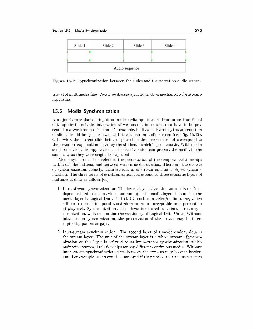
Section 15.6. Media Synchronization 573
Slide 1 Slide 2 Slide 3 Slide 4
Audio sequence
Figure 15.12. Synchronization between the slides and the narration audio stream.
trieval of multimedia �les. Next, we discuss synchronization mechanisms for stream-
ing media.
15.6 Media Synchronization
A major feature that distinguishes multimedia applications from other traditional
data applications is the integration of various media streams that have to be pre-
sented in a synchronized fashion. For example, in distance learning, the presentation
of slides should be synchronized with the narration audio stream (see Fig. 15.12).
Otherwise, the current slide being displayed on the screen may not correspond to
the lecturer's explanation heard by the students, which is problematic. With media
synchronization, the application at the receiver side can present the media in the
same way as they were originally captured.
Media synchronization refers to the preservation of the temporal relationships
within one data stream and between various media streams. There are three levels
of synchronization, namely, intra-stream, inter-stream and inter-object synchro-
nization. The three levels of synchronization correspond to three semantic layers of
multimedia data as follows [66].
1. Intra-stream synchronization: The lowest layer of continuous media or time-
dependent data (such as video and audio) is the media layer. The unit of the
media layer is Logical Data Unit (LDU) such as a video/audio frame, which
adheres to strict temporal constraints to ensure acceptable user perception
at playback. Synchronization at this layer is referred to as intra-stream syn-
chronization, which maintains the continuity of Logical Data Units. Without
intra-stream synchronization, the presentation of the stream may be inter-
rupted by pauses or gaps.
2. Inter-stream synchronization: The second layer of time-dependent data is
the stream layer. The unit of the stream layer is a whole stream. Synchro-
nization at this layer is referred to as inter-stream synchronization, which
maintains temporal relationships among di�erent continuous media. Without
inter-stream synchronization, skew between the streams may become intoler-
ant. For example, users could be annoyed if they notice that the movements
574 Streaming Video over the Internet and Wireless IP Networks Chapter 15
of the lips of a speaker do not correspond to the presented audio.
3. Inter-object synchronization: The highest layer of a multimedia document is
the object layer, which integrates streams and time-independent data such
as text and still images. Synchronization at this layer is referred to as inter-
object synchronization. The objective of inter-object synchronization is to
start and stop the presentation of the time-independant data within a tolerable
time interval, if some previously de�ned points of the presentation of a time-
dependent media object are reached. Without inter-object synchronization,
for example, the audience of a slide show could be annoyed if the audio is
commenting one slide while another slide is being presented.
Media streams may lose synchronization after moving from the server to the
client. As shown in Fig. 15.1, there are many components in the path transporting
data from its storage site to the user. Speci�cally, the server retrieves data from
the storage device and sends that data into the network; the network transports the
data to the client; the client reads the data from its network interface and presents it
to the user; operating systems and protocols allow these systems to run and do their
work. Each of these components on the transport path performs a certain task and
a�ects the data in a di�erent way. They all inevitably introduce delays and delay
variations in either predictable or unpredictable manners. In particular, the delay
introduced in the network is typically unpredictable due to the best-e�ort nature of
the Internet. The incurred delays and delay variations could disrupt intra-media,
inter-media, and inter-object synchronization. Therefore, media synchronization
mechanisms are required to ensure proper rendering of the multimedia presentation
at the client.
The essential part of any media synchronization mechanism is the speci�cations
of the temporal relations within a medium and between the media. The temporal re-
lations can be speci�ed either automatically or manually. In the case of audio/video
recording and playback, the relations are speci�ed automatically by the recording
device. In the case of presentations that are composed of independently captured or
otherwise created media, the temporal relations have to be speci�ed manually (with
human intervention). The manual speci�cation can be illustrated by the design of a
slide show: the designer selects the appropriate slides, creates an audio object and
de�nes the segments of the audio stream where the slides have to be presented (see
Fig. 15.12).
The methods that are used to specify the temporal relations include interval-
based, axes-based, control ow-based, and event-based speci�cations [7]. A widely-
used speci�cation method for continuous media is axes-based speci�cations or time-
stamping: at the source, a stream is time-stamped to keep temporal information
within the stream and with respect to other streams; at the destination, the appli-
cation presents the streams according to their temporal relation.
Besides specifying the temporal relations, it is desirable that synchronization
is supported by each component on the transport path. For example, the servers
store large amount of data in such a way that retrieval is quick and eÆcient to
Section 15.6. Media Synchronization 575
reduce delay; the network provides suÆcient bandwidth, and delay and jitter intro-
duced by the network are tolerable to the multimedia applications; the operating
systems and the applications provide real-time data processing (e.g., retrieval, re-
synchronization, and display). However, real-time support from the network is
not available in the current Internet. Hence, most synchronization mechanisms
are based on the end systems. These synchronization mechanisms can be either
preventive or corrective [36].
� Preventive mechanisms are designed to minimize synchronization errors as
data are transported from the server to the user. In other words, preventive
mechanisms attempt to minimize latencies and jitters. These mechanisms
involve disk-reading scheduling algorithms, network transport protocols, op-
erating systems and synchronization schedulers. Disk-reading scheduling is
the process of organizing and coordinating the retrieval of data from the
storage devices. Network transport protocols provide means for preserving
synchronization during data transmission over the Internet. Operating sys-
tems achieve the precise control of timing constraints by using EDF or rate
monotonic scheduling. A synchronization scheduler can use the synchroniza-
tion speci�cations for a presentation to create a schedule for the delivery of
the media streams to the client by the servers (delivery schedule) and the
presentation of these media streams to the user by the client application (pre-
sentation schedule). This scheduler can be centralized (entirely located at
the client) or distributed (the delivery scheduling functionalities are shared
among the servers and the client).
� Corrective mechanisms are designed to recover synchronization in presence
of synchronization errors. Synchronization errors are unavoidable since the
Internet introduces random delay. Random delay destroys the continuity of
the media stream by producing gaps and jitters during the data transmission.
Therefore, certain compensations (i.e., corrective mechanisms) at the receiver
are necessary when synchronization errors occur.
An example of corrective mechanisms is the Stream Synchronization Protocol
(SSP) [25]. In SSP, the concept of an \intentional delay" is used by the various
streams in order to adjust their presentation time to recover from network
delay variations. The operations of the Stream Synchronization Protocol are
described as follows. At the client side, units that control and monitor the
client-end of the data connections compare the real arrival times of data with
the ones predicted by the presentation schedule and notify the scheduler of
any discrepancies. These discrepancies are then compensated by the scheduler,
which delays the display of data that are \ahead" of other data, allowing the
late data to \catch up".
In sum, media synchronization is one of the key issues in the design of media
streaming services. A great deal of e�ort has been contributed in the synchro-
nization area. As an overview of this area, we have described the synchronization
576 Streaming Video over the Internet and Wireless IP Networks Chapter 15
concepts, requirements and approaches. For more information on media synchro-
nization, please refer to [7, 66] and references therein. Next, we describe the proto-
cols for streaming video.
15.7 Protocols for Streaming Video
Protocols are designed and standardized for communication between clients and
streaming servers. According to their functionalities, the protocols directly related
to streaming video over the Internet can be classi�ed into three categories:
1. Network-layer protocol: The network-layer protocol provides basic net-
work service support such as network addressing. The Internet Protocol (IP)
serves as the network-layer protocol for Internet video streaming.
2. Transport protocol: Transport protocols provide end-to-end network trans-
port functions for streaming applications. These protocols include User Data-
gram Protocol (UDP), Transmission Control Protocol (TCP), Real-time Trans-
port Protocol (RTP), and Real-Time Control Protocol (RTCP). UDP and
TCP are lower-layer transport protocols while RTP and RTCP [59] are upper-
layer transport protocols, which are implemented on top of UDP/TCP (see
Fig. 15.13).
3. Session control protocol: A session control protocol de�nes the messages
and procedures to control the delivery of the multimedia data during an es-
tablished session. The Real-Time Streaming Protocol (RTSP) [61] is such a
session control protocol.
To illustrate the relations among the three types of protocols, we depict the
protocol stacks for media streaming in Fig. 15.13. As shown in Fig. 15.13, at
the sending side, the compressed video/audio data is retrieved and packetized at
the RTP layer. The RTP-packetized streams provide timing and synchronization
information, as well as sequence numbers. The RTP-packetized streams are then
passed to the UDP/TCP layer and the IP layer. The resulting IP packets are
transported over the Internet. At the receiver side, the media streams are processed
in the reversed manner before their presentations. This is the case for the data
plane. For the control plane, RTCP packets and RTSP packets are multiplexed at
the UDP/TCP layer and move to the IP layer for transmission over the Internet.
The rest of this section is organized as follows. In Section 15.7.1, we discuss
transport protocols for streaming media. Section 15.7.2 describes the session control
protocol, i.e., RTSP.
15.7.1 Transport Protocols
The transport protocol family for media streaming includes UDP, TCP, RTP, and
RTCP protocols. UDP and TCP provide basic transport functions while RTP and
RTCP run on top of UDP/TCP.
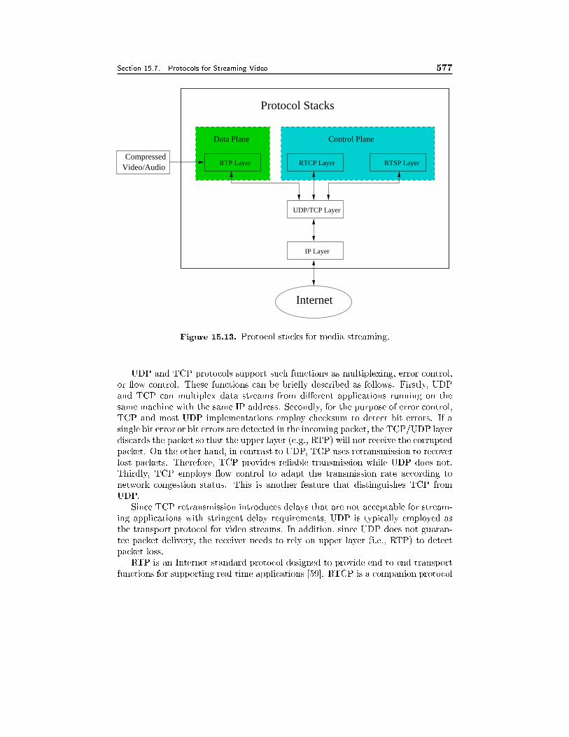
Section 15.7. Protocols for Streaming Video 577
UDP/TCP Layer
IP Layer
Internet
RTP Layer RTCP Layer RTSP LayerCompressed
Video/Audio
Data Plane Control Plane
Protocol Stacks
Figure 15.13. Protocol stacks for media streaming.
UDP and TCP protocols support such functions as multiplexing, error control,
or ow control. These functions can be brie y described as follows. Firstly, UDP
and TCP can multiplex data streams from di�erent applications running on the
same machine with the same IP address. Secondly, for the purpose of error control,
TCP and most UDP implementations employ checksum to detect bit errors. If a
single bit error or bit errors are detected in the incoming packet, the TCP/UDP layer
discards the packet so that the upper layer (e.g., RTP) will not receive the corrupted
packet. On the other hand, in contrast to UDP, TCP uses retransmission to recover
lost packets. Therefore, TCP provides reliable transmission while UDP does not.
Thirdly, TCP employs ow control to adapt the transmission rate according to
network congestion status. This is another feature that distinguishes TCP from
UDP.
Since TCP retransmission introduces delays that are not acceptable for stream-
ing applications with stringent delay requirements, UDP is typically employed as
the transport protocol for video streams. In addition, since UDP does not guaran-
tee packet delivery, the receiver needs to rely on upper layer (i.e., RTP) to detect
packet loss.
RTP is an Internet standard protocol designed to provide end-to-end transport
functions for supporting real-time applications [59]. RTCP is a companion protocol
578 Streaming Video over the Internet and Wireless IP Networks Chapter 15
to RTP. RTCP is designed to provide QoS feedback to the participants of an RTP
session. In order words, RTP is a data transfer protocol while RTCP is a control
protocol.
RTP does not guarantee QoS or reliable delivery, but rather, provides the fol-
lowing functions in support of media streaming:
� Time-stamping: RTP provides time-stamping so that time-stamps can be
used to synchronize di�erent media streams. Note that RTP itself is not
responsible for the synchronization. This has to be done by the applications.
� Sequence numbering: Since packets arriving at the receiver may be out of
sequence (UDP does not deliver packets in sequence), RTP employs sequence
numbering to place the incoming RTP packets in the correct order. The
sequence numbers are also used for packet loss detection.
� Payload type identi�cation: The type of the payload contained in an RTP
packet is indicated by an RTP-header �eld called payload type identi�er. The
receiver interprets the content of the packet based on the payload type identi-
�er. Certain common payload types such as MPEG-1/2 audio and video have
been assigned payload type numbers [60]. For other payloads, this assignment
can be done with session control protocols.
� Source indenti�cation: The source of each RTP packet is identi�ed by
an RTP-header �eld called Synchronization SouRCe identi�er (SSRC). SSRC
provides a means for the receiver to distinguish di�erent sources.
RTCP is the control protocol designed to work in conjunction with RTP [59]. In
an RTP session, participants periodically send RTCP packets to convey feedback on
quality of data delivery and information of membership. Basically, RTCP provides
the following services:
� QoS feedback: This is the primary function of RTCP. RTCP provides feed-
back to an application about the quality of data distribution. The control
information is useful to the senders, the receivers and third-party monitors.
The sender can adjust its transmission rate based on the receiver report feed-
back (see Section 15.3.1). The receivers can determine whether a congestion
is local, regional or global. Network managers can evaluate the network per-
formance for multicast distribution.
RTCP provides QoS feedback through the use of Sender Reports and Receiver
Reports at the source and destination, respectively. The reports can contain
information on the quality of reception such as (1) fraction of the lost RTP
packets since the last report, (2) cumulative number of lost packets since
the beginning of reception, (3) packet interarrival jitter, and (4) delay since
receiving the last sender's report.
� Participant identi�cation: A source can be identi�ed by the SSRC �eld
in the RTP header. But the SSRC identi�er is not convenient for human
Section 15.7. Protocols for Streaming Video 579
users. To remedy this problem, RTCP provides a human-friendly mecha-
nism for source identi�cation. Speci�cally, RTCP SDES (source description)
packets contain textual information called canonical names as globally unique
identi�ers of the session participants. It may include user's name, telephone
number, email address and other information.
� Control packets scaling:
To scale the RTCP control packet transmission with the number of partic-
ipants, a control mechanism is designed as follows. The control mechanism
keeps the total control packets to 5% of the total session bandwidth. Among
the control packets, 25% are allocated to the Sender Reports and 75% to the
Receiver Reports. To prevent control packet starvation, at least 1 control
packet is sent within 5 seconds at the sender or receiver.
� Inter-media synchronization: RTCP Sender Reports contain an indication
of real time and the corresponding RTP timestamp. This can be used in inter-
media synchronization like lip synchronization in video.
� Minimal session control information: This optional functionality can be
used for transporting session information such as names of the participants.
15.7.2 Session Control Protocol: RTSP
The Real-Time Streaming Protocol (RTSP) is a session control protocol for stream-
ing media over the Internet [61]. One of the main functions of RTSP is to support
VCR-like control operations such as stop, pause/resume, fast forward and fast re-
verse. In addition, RTSP also provides means for choosing delivery channels (e.g.,
UDP, multicast UDP or TCP), and delivery mechanisms based upon RTP. RTSP
works for multicast as well as unicast.
Another main function of RTSP is to establish and control streams of continuous
audio and video media between the media servers and the clients. Speci�cally, RTSP
provides the following operations:
1. Media retrieval: The client can request a presentation description, and ask
the server to setup a session to send the requested media data.
2. Inviting a media server to a conference: The media server can be invited
to the conference to play back media or to record a presentation.
3. Adding media to an existing session: The server or the client can notify
each other about any additional media becoming available to the established
session.
RTSP is intended to provide the same services on streamed audio and video
as HTTP does for text and graphics (HTTP: HyperText Transfer Protocol). It is
designed to have similar syntax and operations so that most extension mechanisms
to HTTP can be added to RTSP.
580 Streaming Video over the Internet and Wireless IP Networks Chapter 15
In RTSP, each presentation and media stream is identi�ed by an RTSP URL
(URL: Univeral Resource Locator). The overall presentation and the properties
of the media are de�ned in a presentation description �le, which may include the
encoding, language, RTSP URLs, destination address, port, and other parameters.
The presentation description �le can be obtained by the client using HTTP, email
or other means.
In sum, RTSP is designed to initiate and direct delivery of streaming media data
from media servers; RTP is a transport protocol for streaming media data; RTCP
is a protocol for monitoring delivery of RTP packets; UDP and TCP are lower-
layer transport protocols for RTP/RTCP/RTSP packets; IP provides a means for
delivering UDP/TCP packets over the Internet. The combination of these protocols
provides a complete streaming service over the Internet.
15.8 Streaming Video over Wireless IP Networks
Recently, the emergence of broadband wireless networks has brought great interest
in real-time video communications over wireless IP networks. However, delivering
quality video over wireless networks in real-time is a challenging task. This is
primarily because of the following problems.
Bandwidth uctuations: First, the throughput of a wireless channel may be
reduced due to multipath fading, co-channel interference, and noise distur-
bances. Second, the capacity of a wireless channel may uctuate with the
changing distance between the base station and the mobile host. Third, when
a mobile terminal moves between di�erent networks (e.g., from wireless local
area network to wireless wide area network), the available bandwidth may
vary drastically (e.g., from a few megabits per second to a few kilobits per
second). Finally, when a hando� takes place, a base station may not have
enough unused radio resource to meet the demand of a newly joined mobile
host. As a result, bandwidth uctuation is a serious problem for real-time
video transmission over wireless networks.
High bit error rate: Compared with the wired links, wireless channels are typi-
cally much more noisy and have both small-scale (multipath) and large-scale
(shadowing) fades, making the bit error rate (BER) very high. The resulting
bit errors can have devastating e�ect on video presentation quality. Therefore,
there is a critical need for robust transmission of video over wireless channels.
Heterogeneity: In a multicast scenario, receivers may have di�erent requirements
and properties in terms of latency, visual quality, processing capabilities,
power limitations (wireless vs. wired) and bandwidth limitations. The het-
erogeneous nature of receivers' requirements and properties make it diÆcult
to design an eÆcient multicast mechanism.
It has been shown that scalable video is capable of coping gracefully with the
variability of bandwidth [2, 45]. A scalable video coding scheme produces a com-
Section 15.8. Streaming Video over Wireless IP Networks 581
pressed bit-stream, parts of which are decodable. Compared with decoding the
complete bit-stream, decoding part of the compressed bit-stream produces pictures
with degraded quality, or smaller image size, or smaller frame rate [18]. In contrast,
non-scalable video is more susceptible to bandwidth uctuations since it cannot
adapt its video representation to bandwidth variations [45]. Thus, scalable video
is more suitable for use in a wireless environment to cope with the uctuation of
wireless channels. Furthermore, scalable video representation is a good solution to
the heterogeneity problem in multicast case [45].
Recently, application-aware adaptive services have been demonstrated to be able
to e�ectively mitigate uctuations of resource availability in wireless networks [2].
Scalable video representation naturally �ts unequal error protection, which can
e�ectively combat bit errors induced by the wireless medium. This motivates us
to present an adaptive framework to support quality video communication over
wireless IP networks.
For transporting video over wireless, there have been many proposals of adap-
tive approaches and services in the literature, which include an \adaptive reserved
service" framework [38], an adaptive service based on QoS bounds and revenue [44],
an adaptive framework targeted at end-to-end QoS provisioning [49], a utility-fair
adaptive service [6], a framework for soft QoS control [57], a teleservice model based
on an adaptive QoS paradigm [33], an adaptive QoS management architecture [37],
and an adaptive framework for scalable video over wireless IP networks [84].
In this section, we present an adaptive framework [85] for future QoS-enabled
wireless IP networks. The adaptive framework consists of (1) scalable video repre-
sentations, each of which has its own speci�ed QoS requirement, (2) network-aware
applications, which are aware of network status, and (3) adaptive services, which
make network elements support the QoS requirements of scalable video represen-
tations. Under this framework, as wireless channel conditions change, the mobile
terminal and network elements can scale the video streams and transport the scaled
video streams to receivers with acceptable perceptual quality. The adaptive frame-
work has the following key features.
1. Graceful quality degradation: Di�erent from non-scalable video, scalable video
can adapt its video representation to bandwidth variations and the network
can drop packets with awareness of the video representations. As a result,
perceptual quality is gracefully degraded under severe channel conditions.
2. EÆciency: When there is excess bandwidth (excluding reserved bandwidth),
the excess bandwidth will be eÆciently used in a way that maximizes the
perceptual quality or revenue.
3. Fairness: The resources can be shared in either a utility-fair manner [6] or a
max-min fair manner [44].
The remainder of this section is organized as follows. Section 15.8.1 describes
network-aware applications. In Section 15.8.2, we present the adaptive services for
transporting scalable video over wireless IP networks.
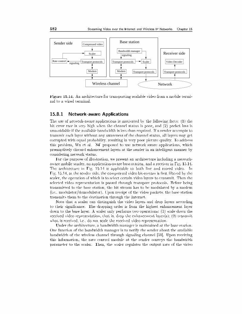
582 Streaming Video over the Internet and Wireless IP Networks Chapter 15
Transport protocols
Modem
Wireless channel
Transport protocols Scaler
Modem Transport protocols
Bandwidth manager
Network
Transport protocols
Rate control
Base stationCompressed video
signaling
signalingScaler
Video Decoder
Receiver side
Sender side
Figure 15.14. An architecture for transporting scalable video from a mobile termi-
nal to a wired terminal.
15.8.1 Network-aware Applications
The use of network-aware applications is motivated by the following facts: (1) the
bit error rate is very high when the channel status is poor, and (2) packet loss is
unavoidable if the available bandwidth is less than required. If a sender attempts to
transmit each layer without any awareness of the channel status, all layers may get
corrupted with equal probability, resulting in very poor picture quality. To address
this problem, Wu et al. [84] proposed to use network-aware applications, which
preemptively discard enhancement layers at the sender in an intelligent manner by
considering network status.
For the purpose of illustration, we present an architecture including a network-
aware mobile sender, an application-aware base station, and a receiver in Fig. 15.14.
The architecture in Fig. 15.14 is applicable to both live and stored video. In
Fig. 15.14, at the sender side, the compressed video bit-stream is �rst �ltered by the
scaler, the operation of which is to select certain video layers to transmit. Then the
selected video representation is passed through transport protocols. Before being
transmitted to the base station, the bit-stream has to be modulated by a modem
(i.e., modulator/demodulator). Upon receipt of the video packets, the base station
transmits them to the destination through the Internet.
Note that a scaler can distinguish the video layers and drop layers according
to their signi�cance. The dropping order is from the highest enhancement layer
down to the base layer. A scaler only performs two operations: (1) scale down the
received video representation, that is, drop the enhancement layer(s); (2) transmit
what is received, i.e., do not scale the received video representation.
Under the architecture, a bandwidth manager is maintained at the base station.
One function of the bandwidth manager is to notify the sender about the available
bandwidth of the wireless channel through signaling channel [50]. Upon receiving
this information, the rate control module at the sender conveys the bandwidth
parameter to the scaler. Then, the scaler regulates the output rate of the video
Section 15.8. Streaming Video over Wireless IP Networks 583
stream so that the transmission rate is less than or equal to the available bandwidth.
Another scenario is that the base station noti�es the sender about the channel
quality (i.e., BER) [3]. Upon receiving this information, the rate control module at
the sender commands the scaler to perform the following (suppose that the video
is compressed into two layers): (1) if the BER is above a threshold, discard the
enhancement layer so that the bandwidth allocated for the enhancement layer can
be utilized by forward error correction (FEC) to protect the base layer; (2) otherwise
transmit both layers.
The network-aware application has two advantages. Firstly, by taking the avail-
able bandwidth into account, the sender can make the best use of network resources
by selectively discarding enhancement layers in order to minimize the likelihood of
more signi�cant layers being corrupted, thereby increasing the perceptual quality
of the video delivered. Secondly, by considering the channel error status, the sender
can discard the enhancement layers and FEC can utilize the bandwidth allocated for
the enhancement layer to protect the base layer, thereby maximizing the possibility
of the base layer being correctly received.
Note that adaptive techniques at the physical/link layer are required to sup-
port network-aware applications. Such adaptive techniques include a combination
of variable spreading, coding, and code aggregation in Code Division Multiple Ac-
cess (CDMA) systems, adaptive coding and modulation in Time Division Multiple
Access (TDMA) systems, channel quality estimation, and measurement feedback
channel [50]. In addition, the feedback interval is typically constrained to be on the
order of tens to hundreds of milliseconds [50].
15.8.2 Adaptive Service
A scalable video encoder can generate multiple layers or substreams to the network.
The adaptive service is to provide scaling of the substreams based on the resource
availability conditions in the �xed and wireless network. Speci�cally, the adaptive
service includes the following functions.
� Reserve a minimum bandwidth to meet the demand of the base layer. As a
result, the perceptual quality can always be achieved at an acceptable level.
� Adapt the enhancement layers based on the available bandwidth and the
fair policy. In other words, it scales the video streams based on resource
availability.
Advantages of using scaling inside the network include:
(1) Adaptivity to network heterogeneity. For example, when an upstream link
with larger bandwidth feeds a downstream link with smaller bandwidth, use of a
scaler at the connection point could help improve the video quality. This is because
the scaler can selectively drop substreams instead of randomly dropping packets.
(2) Low latency and low complexity. Scalable video representations make the
operation at a scaler very simple, i.e., only discarding enhancement layers. Thus,
the processing is fast, compared with processing on non-scalable video.
584 Streaming Video over the Internet and Wireless IP Networks Chapter 15
(3) Lower call blocking and hando� dropping probability. The adaptability of
scalable video at base stations can translate into lower call blocking prabability and
hando� dropping probability.
The adaptive service can be deployed in the whole network (i.e., end-to-end pro-
visioning) or only at base stations (i.e., local provisioning). Since local provisioning
of the adaptive service is just a subset of end-to-end provisioning, we will focus on
end-to-end provisioning.
The required components of the end-to-end adaptive service include: (1) service
contract, (2) call admission control and resource reservation, (3) mobile multicast
mechanism, (4) substream scaling, (5) substream scheduling, and (6) link-layer error
control. These are described in more detail below.
Service contract
The service contract between the application and the network could consist of multi-
ple subcontracts, each of which corresponds to one or more substreams with similar
QoS guarantees. Each subcontract has to specify traÆc characteristics and QoS
requirements of the corresponding substream(s). A typical scenario is that a sub-
contract for the base layer speci�es reserved bandwidth while a subcontract for the
enhancement layers does not specify any QoS guarantee.
At a video source, substreams must be generated according to subcontracts used
by the application and shaped at the network access point. In addition, a substream
is assigned a priority according to its signi�cance. For example, the base layer is
assigned the highest priority. The priority can be used by routing, scheduling,
scaling, and error control components of the adaptive network.
15.8.3 Call admission control and resource reservation
Call admission control (CAC) and resource reservation are two of the major com-
ponents in end-to-end QoS provisioning. The function of CAC is to check whether
admitting the incoming connection would reduce the service quality of existing con-
nections, and whether the incoming connection's QoS requirements can be met. If
a connection request is accepted, resources need to be reserved for this connection
in two parts. First of all, in order to maintain the speci�ed QoS over a long time-
scale, the network must reserve some resources along the current path of a mobile
connection. Second, in order to seamlessly achieve the QoS at a short time-scale,
some duplication must be done in the transport of the connection to neighboring
base stations of a connection so that in the event of a hando�, an outage in the link
can be avoided.
The scalable video representation (i.e., substream) concept provides a very ex-
ible and eÆcient solution to the problem of CAC and resource reservation. First,
there is no need to reserve bandwidth for the complete stream since typically only
base-layer substream needs QoS guarantee. As a result, CAC is only based on the
requirement of the base layer and resource is reserved only for the base-layer sub-
stream. Second, the enhancement layer substream(s) of one connection could share
Section 15.8. Streaming Video over Wireless IP Networks 585
the leftover bandwidth with the enhancement-layer substreams of other connec-
tions. The enhancement-layer substreams are subject to scaling under bandwidth
shortage and/or severe error conditions, which will be discussed in Section 15.8.3.
Mobile multicast mechanism
CAC and resource reservation can provide connection-level QoS guarantee. To
seamless guarantee QoS at packet level, mobile multicast mechanism has to be
used. That is, while being transported along its current path, the base-layer stream
is also multicast to its neighboring base stations so that QoS at a small time-scale
can be seamlessly achieved.
To support seamless QoS, the mobile routing protocol needs to be proactive
and anticipatory in order to match the delay, loss, and jitter constraints of a sub-
stream. According to the requirements of a substream, multicast paths might need
to be established. The multicast paths terminate at base stations that are potential
access-point candidates of a mobile terminal. The coverage of such a multicast path
depends on the QoS requirements and the mobility as well as hando� characteristics
of a mobile receiver. As a mobile station hands o� from a base station to another,
new paths are added and old paths are deleted [49].
Substream scaling
Scaling is employed during bandwidth uctuations and/or under poor channel con-
ditions. As the available bandwidth on a path desreases due to mobility or fading,
lower-priority substreams are dropped by the scaler(s) on the path and substreams
with higher priority are transmitted. As more bandwidth becomes available, lower-
priority substreams are passed through the scaler, and the perceptual quality at
the receivers increases. Figure 15.14 shows an architecture for transporting scalable
video from a mobile terminal to a wired terminal. Figure 15.15 depicts an archi-
tecture for transporting scalable video from a wired terminal to a mobile terminal.
We do not show the case of transporting scalable video from a mobile terminal to
a mobile terminal since it is a combination of Fig. 15.14 and Fig. 15.15.
The scaling decision is made by a bandwidth manager. When there is no excess
bandwidth (excluding reserved bandwidth), the bandwidth manager instructs the
scaler to drop the enhancement layers. If there is excess bandwidth, the excess
bandwidth can be shared in either a utility-fair manner [6] or a max-min fair manner
[44].
Substream scheduling
The substream scheduler is used in mobile terminals as well as base stations. Its
function is to schedule the transmission of packets on the wireless medium according
to their substream QoS speci�cations and priorities.
When a short fading period is observed, a mobile terminal tries to prioritize the
transmission of its substreams in order to achieve a minimum QoS. Here, depending
on channel conditions, a substream might be dropped for a period of time in order
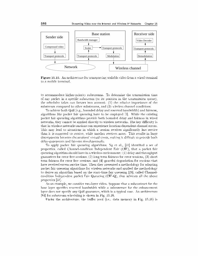
586 Streaming Video over the Internet and Wireless IP Networks Chapter 15
Transport protocols Transport protocols
Transport protocols Transport protocols
Wireless channelNetwork
Bandwidth manager
Scaler
Modulation
Base station
Compressed video
Demodulation
Video DecoderSender side
Receiver side
Figure 15.15. An architecture for transporting scalable video from a wired terminal
to a mobile terminal.
to accommodate higher-priority substreams. To determine the transmission time
of any packet in a speci�c substream (or its position in the transmission queue),
the scheduler takes two factors into account: (1) the relative importance of the
substream compared to other substreams, and (2) wireless channel conditions.
To achieve both QoS (e.g., bounded delay and reserved bandwidth) and fairness,
algorithms like packet fair queueing have to be employed [5]. While the existing
packet fair queueing algorithms provide both bounded delay and fairness in wired
networks, they cannot be applied directly to wireless networks. The key diÆculty is
that in wireless networks sessions can experience location-dependent channel errors.
This may lead to situations in which a session receives signi�cantly less service
than it is supposed to receive, while another receives more. This results in large
discrepancies between the sessions' virtual times, making it diÆcult to provide both
delay-guarantees and fairness simultaneously.
To apply packet fair queueing algorithms, Ng et al., [51] identi�ed a set of
properties, called Channel-condition Independent Fair (CIF), that a packet fair
queueing algorithm should have in a wireless environment: (1) delay and throughput
guarantees for error-free sessions, (2) long term fairness for error sessions, (3) short
term fairness for error-free sessions, and (4) graceful degradation for sessions that
have received excess service time. Then they presented a methodology for adapting
packet fair queueing algorithms for wireless networks and applied the methodology
to derive an algorithm based on the start-time fair queueing [28], called Channel-
condition Independent packet Fair Queueing (CIF-Q), that achieves all the above
properties [51].
As an example, we consider two-layer video. Suppose that a subcontract for the
base layer speci�es reserved bandwidth while a subcontract for the enhancement
layer does not specify any QoS guarantee, which is a typical case. An architecture
[84] for substream scheduling is shown in Fig. 15.16.
Under the architecture, the bu�er pool (i.e., data memory in Fig. 15.16) is
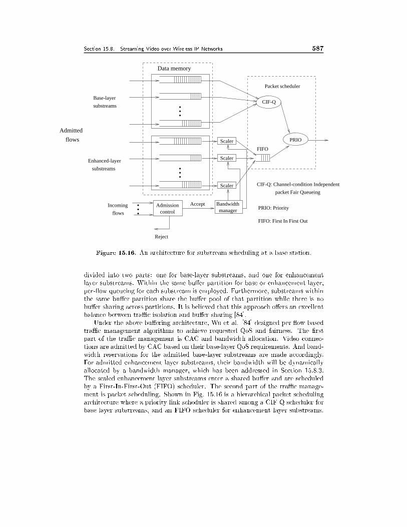
Section 15.8. Streaming Video over Wireless IP Networks 587
controlPRIO: Priority
packet Fair Queueing
CIF-Q: Channel-condition Independent
Admission
FIFO
Reject
Acceptmanager
Bandwidth
PRIO
CIF-Q
FIFO: First In First Out
substreams
Scaler
Incoming
Scaler
Scaler
substreams
...
...
Base-layer
.
Packet scheduler
.
flows
.Enhanced-layer
Admitted
flows
Data memory
Figure 15.16. An architecture for substream scheduling at a base station.
divided into two parts: one for base-layer substreams, and one for enhancement
layer substreams. Within the same bu�er partition for base or enhancement layer,
per- ow queueing for each substream is employed. Furthermore, substreams within
the same bu�er partition share the bu�er pool of that partition while there is no
bu�er sharing across partitions. It is believed that this approach o�ers an excellent
balance between traÆc isolation and bu�er sharing [84].
Under the above bu�ering architecture, Wu et al. [84] designed per- ow based
traÆc management algorithms to achieve requested QoS and fairness. The �rst
part of the traÆc management is CAC and bandwidth allocation. Video connec-
tions are admitted by CAC based on their base-layer QoS requirements. And band-
width reservations for the admitted base-layer substreams are made accordingly.
For admitted enhancement layer substreams, their bandwidth will be dynamically
allocated by a bandwidth manager, which has been addressed in Section 15.8.3.
The scaled enhancement layer substreams enter a shared bu�er and are scheduled
by a First-In-First-Out (FIFO) scheduler. The second part of the traÆc manage-
ment is packet scheduling. Shown in Fig. 15.16 is a hierarchical packet scheduling
architecture where a priority link scheduler is shared among a CIF-Q scheduler for
base-layer substreams, and an FIFO scheduler for enhancement layer substreams.
588 Streaming Video over the Internet and Wireless IP Networks Chapter 15
Service priority is �rst given to the CIF-Q scheduler and then to the FIFO scheduler.
Link-layer error control
To provide quality video over wireless channels, link-layer error control is required.
Basically, there are two kinds of error control mechanisms, namely, forward error
correction (FEC) and automatic repeat request (ARQ). The disadvantage of FEC
is that it is not adaptive to varying channel conditions and it works only when
the BER is below the FEC code's recovery capability. The disadvantage of ARQ
is unbounded delay; that is, in the worst case, a packet may be retransmitted an
unlimited number of times to recover from bit errors.
To address the problems associated with FEC and ARQ, truncated type-II hy-
brid ARQ schemes [41, 89] and delay-constrained hybrid ARQ [82] have been pro-
posed. These hybrid ARQ schemes combine the good features of FEC and ARQ:
bounded delay and adaptiveness. On the other hand, unequal error protection [30]
naturally �t the hierarchical structure of scalable video. Speci�cally, the base layer
can be better protected against transmission errors than the enhancement layers.
This form of unequal error protection is much more desirable than having to protect
all the substreams. An open issue is how to combine unequal error protection with
the hybrid ARQ schemes [85].
15.9 Summary
In this chapter, we have surveyed major approaches and mechanisms for Internet
video streaming and have presented an adaptive framework for video over wireless
IP. The objective is not to provide an exhaustive review of existing approaches
and mechanisms, but instead to give the reader a perspective on the range of op-
tions available and the associated trade-o�s among performance, functionality, and
complexity.
We would like to stress that the seven areas (i.e., video compression, application-
layer QoS control, continuous media distribution services, streaming servers, media
synchronization mechanisms, protocols, video over wireless IP) are basic building
blocks for a streaming video architecture. Built with the seven basic building blocks,
the streaming video architecture ties together a broad range of signal processing,
networking and server technologies. Therefore, a thorough understanding of the
whole architecture for streaming video is bene�cial for developing signal process-
ing techniques (e.g., scalable video compression) suitable for streaming video. In
addition, in-depth knowledge on both signal processing and networking helps to
make e�ective design and use of application-layer QoS control, continuous media
distribution services, protocols and services for video over wireless IP. Furthermore,
the architectural understanding is instrumental in the design of eÆcient, scalable,
and/or fault-tolerant streaming servers.
Section 15.10. Bibliography 589
15.10 Bibliography
[1] A. Albanese, J. Bl�omer, J. Edmonds, M. Luby, M. Sudan, \Priority encod-
ing transmission," IEEE Trans. on Information Theory (special issue on coding
theory), vol. 42, no. 6, Nov. 1996.
[2] A. Balachandran, A.T. Campbell, and M.E. Kounavis, \Active �lters: delivering
scalable media to mobile devices," Proc. Seventh International Workshop on Net-
work and Operating System Support for Digital Audio and Video (NOSSDAV'97),
May 1997.
[3] K. Balachandran, S. Kadaba, and S. Nanda, \Rate adaptation over mobile
radio channels using channel quality information," Proc. IEEE GLOBECOM'98,
Nov. 1998.
[4] S. Berson, L. Golubchik, and R. R. Muntz, \Fault tolerant design of multimedia
servers," Proc. ACM SIGMOD'95, pp. 364{375, May 1995.
[5] V. Bharghavan, S. Lu, and T. Nandagopal, \Fair queuing in wireless networks:
issues and approaches," IEEE Personal Commun. Mag., pp. 44{53, Feb. 1999.
[6] G. Bianchi, A.T. Campbell, and R. Liao, \On utility-fair adaptive ser-
vices in wireless networks," 6th International Workshop on Quality of Service
(IWQOS'98), Napa Valley, CA, May 1998.
[7] G. Blakowski and R. Steinmetz, \A media synchronization Survey: reference
model, speci�cation, and case studies," IEEE Journal on Selected Areas in Com-
munications, vol. 14, no. 1, pp. 5{35, Jan. 1996.
[8] J-C. Bolot, T. Turletti, I. Wakeman, \Scalable feedback control for multicast
video distribution in the Internet," Proc. ACM SIGCOMM'94, pp. 58{67, London,
UK, Sept. 1994.
[9] Y.-C. Chang, D. G. Messerschmitt, T. Carney, and S. A. Klein, \Delay cognizant
video coding: architecture, applications, and quality evaluations," to appear in
IEEE Trans. Image Processing.
[10] Y.-C. Chang and D. G. Messerschmitt, \Adaptive layered video coding for
multi-time scale bandwidth uctuations," submitted to IEEE Journal on Selected
Areas in Communications.
[11] A. Chankhunthod, P. Danzig, C. Neerdaels, M. F. Schwartz, and K. J. Worrell,
\A hierarchical Internet object cache," Proc. USENIX 1996 Annual Technical
Conference, Jan. 1996.
[12] M. Chen, D. D. Kandlur, and P. S. Yu, \Support for fully interactive playout in
a disk-array-based video server," Proc. ACM Multimedia'94, New York, Oct. 1994.
590 Streaming Video over the Internet and Wireless IP Networks Chapter 15
[13] S. Y. Cheung, M. Ammar, and X. Li, \On the use of destination set grouping
to improve fariness in multicast video distribution," Proc. IEEE INFOCOM'96,
March 1996.
[14] J. Y. Chung, J. W. S. Liu, and K. J. Lin, \Scheduling periodic jobs that allows
imprecise results," IEEE Transactions on Computers, vol. 19, no. 9, pp. 1156{
1173, Sept. 1990.
[15] G. Davis, and J. Danskin, \Joint source and channel coding for Internet image
transmission," Proc. SPIE Conference on Wavelet Applications of Digital Image
Processing XIX, Denver, Aug. 1996.
[16] P. J. Denning, \E�ects of scheduling on �le memory operations," Proc. AFIPS
Spring Joint Computer Conference, Reston, Va., pp. 9{21, 1967.
[17] D. H. C. Du and Y.-J. Lee, \Scalable server and storage architectures for video
streaming," Proc. IEEE International Conference on Multimedia Computing and
Systems, vol. 1, pp. 62{67, June 1999.
[18] T. Ebrahimi and M. Kunt, \Visual data compression for multimedia applica-
tions," Proceedings of the IEEE, vol. 86, no. 6, pp. 1109{1125, June 1998.
[19] A. Eleftheriadis and D. Anastassiou, \Meeting arbitrary QoS constraints using
dynamic rate shaping of coded digital video," Proc. 5th International Workshop
on Network and Operating System Support for Digital Audio and Video (NOSS-
DAV'95), pp. 95{106, April 1995.
[20] L. Fan, P. Cao, J. Almeida and A. Z. Broder, \Summary cache: a scalable
wide-area web cache sharing protocol," IEEE/ACM Trans. on Networking, vol. 8,
no. 3, pp. 281{293, June 2000.
[21] FastForward Networks, \FastForward networks' broadcast overlay architec-
ture," URL: http://www.�net.com/pdfs/boa-whitepaper.pdf.
[22] S. Floyd, and K. Fall, \Promoting the use of end-to-end congestion control
in the Internet," IEEE/ACM Trans. on Networking, vol. 7, no. 4, pp. 458{472,
Aug. 1999.
[23] J. Gafsi and E. W. Biersack, \Performance and reliability study for distributed
video servers: mirroring or parity?" Proc. IEEE International Conference on
Multimedia Computing and Systems, vol. 2, pp. 628{634, June 1999.
[24] J. Gemmell and S. Christodoulakis, \Principles of delay sensitive multimedia
data storage and retrieval," ACM Trans. on Information Systems, vol. 10, no. 1,
pp. 51{90, Jan. 1992.
[25] N. D. Georganas, \Synchronization issues in multimedia presentational and
conversational applications," Proc. Paci�c Workshop on Distributed Multimedia
Systems (DMS'96), June 1996.
Section 15.10. Bibliography 591
[26] M. Ghanbari, \Cell-loss concealment in ATM video codes," IEEE Trans.
Circuits Syst. Video Technol., vol. 3, pp. 238{247, June 1993.
[27] B. Girod, U. Horn, B. Belzer, \Scalable video coding with multiscale motion
compensation and unequal error protection," Proc. Symp. on Multimedia Com-
munications and Video Coding, New York: Plenum Press, pp. 475{482, Oct. 1995.
[28] P. Goyal, H. M. Vin, and H. Chen, \Start-time fair queuing: a scheduling
algorithm for integrated service access," Proc. ACM SIGCOMM'96, Aug. 1996.
[29] A. Guha, \The evolution to network storage architectures for multimedia
applications," Proc. IEEE International Conference on Multimedia Computing
and Systems, vol. 1, pp. 68{73, June 1999.
[30] J. Hagenauer and T. Stockhammer, \Channel coding and transmission aspects
for wireless multimedia," Proceedings of the IEEE, vol. 87, no. 10, pp. 1764{1777,
Oct. 1999.
[31] B. Hamidzadeh and J. Tsun-Ping, \Dynamic scheduling techniques for inter-
active hypermedia servers," IEEE Trans. on Consumer Electronics, vol. 45, no. 1,
Feb. 1999.
[32] M. Hemy, U. Hengartner, P. Steenkiste, and T. Gross, \MPEG system streams
in best-e�ort networks," Proc. Packet Video Workshop'99, New York, April 1999.
[33] A. Iera, A. Molinaro, and S. Marano, \Wireless broadband applications: the
teleservice model and adaptive QoS provisioning," IEEE Communications Maga-
zine, pp. 71{75, Oct. 1999.
[34] K. Illgner and F. Mueller, \Spatially scalable video compression employing
resolution pyramids," IEEE J. Select. Areas Commun., vol. 15, no. 9, pp. 1688{
1703, Dec. 1997.
[35] ISO/IEC JTC 1/SC 29/WG 11, \Information technology { coding of audio-
visual objects, part 1: systems, part 2: visual, part 3: audio," FCD 14496,
Dec. 1998.
[36] J. P. Jarmasz and N. D. Georganas, \Designing a distributed multimedia
synchronization scheduler," Proc. IEEE International Conference on Multimedia
Computing and Systems, pp. 451{457, June 1997.
[37] O. Lataoui, T. Rachidi, L. G. Samuel, S. Gruhl, and R.-H., Yan, \A QoS man-
agement architecture for packet switched 3rd generation mobile systems," Proc.
Networld+Interop 2000 Engineers Conference, May 2000.
[38] K. Lee, \Adaptive network support for mobile multimedia," Proc. ACM Mo-
bicom'95, Nov. 1995.
592 Streaming Video over the Internet and Wireless IP Networks Chapter 15
[39] J. Li, \Visual progressive coding," SPIE Proc. Visual Communications and
Image Processing (VCIP'99), Jan. 1999.
[40] X. Li, S. Paul, M. H. Ammar, \Layered video multicast with retransmis-
sions (LVMR): evaluation of hierarchical rate control," Proc. IEEE INFOCOM'98,
March 1998.
[41] H. Liu and M. El Zarki, \Performance of H.263 video transmission over wireless
channels using hybrid ARQ," IEEE J. on Selected Areas in Communications,
vol. 15, no. 9, pp. 1775{1786, Dec. 1997.
[42] C. L. Liu, and J. W. Layland, \Scheduling algorithms for multiprogramming
in a hard real-time environment," Journal of ACM, vol. 20, no. 1, pp. 46{61,
Jan. 1973.
[43] Y.-J. Liu and Y.-Q. Zhang, \Wavelet-coded image transmission over land
mobile radio channels," IEEE GLOBECOM'92, Orlando, FL, USA, Dec. 1992.
[44] S. Lu, K.-W. Lee and V. Bharghavan, \Adaptive service in mobile computing
environments," 5th International Workshop on Quality of Service (IWQOS'97),
May 1997.
[45] S. McCanne, V. Jacobson, and M. Vetterli, \Receiver-driven layered multi-
cast," Proc. ACM SIGCOMM'96, pp. 117{130, Aug. 1996.
[46] Z. Miao, A. Ortega, \Proxy caching for eÆcient video services over the Inter-
net," Proc. Packet Video'99, April 1999.
[47] J. Moura, R. S. Jasinschi, H. Shiojiri, and J.-C. Lin, \Video over wireless,"
IEEE Personal Communications Magazine, pp. 44{54, Feb. 1996.
[48] A. Mourad, \Doubly-striped disk mirroring: reliable storage for video servers,"
Multimedia, Tools and Applications, vol. 2, pp. 253{272, May 1996.
[49] M. Naghshineh and M. Willebeek-LeMair, \End-to-end QoS provisioning in
multimedia wireless/mobile networks using an adaptive framework," IEEE Com-
munications Magazine, pp. 72{81, Nov. 1997.
[50] S. Nanda, K. Balachandran, and S. Kumar, \Adaptation techniques in wireless
packet data services," IEEE Communications Magazine, pp. 54{64, Jan. 2000.
[51] T.S.E. Ng, I. Stoica and H. Zhang, \Packet fair queueing algorithms for wireless
networks with location-dependent errors," Proc. IEEE INFOCOM'98, pp. 1103{
1111, March 1998.
[52] A. Ortega and K. Ramchandran, \Rate-distortion methods for image and video
compression," IEEE Signal Processing Magazine, pp. 74{90, Nov. 1998.
Section 15.10. Bibliography 593
[53] B. Ozden, R. Rastogi, P. Shenoy and A. Silberschatz, \Fault-tolerant ar-
chitectures for continuous media servers," Proc. ACM SIGMOD'96, pp. 79{90,
June 1996.
[54] R. Puri, K. Ramchandran, K. W. Lee, and V. Bharghavan, \Application of
FEC based multiple description coding to Internet video streaming and multicast,"
Proc. Packet video'2000, May 2000.
[55] H. Radha, Y. Chen, \Fine-granular-scalable video for packet networks," Proc.
Packet Video'99, April 1999.
[56] A. L. Reddy and J. Wyllie, \Disk scheduling in a multimedia I/O system,"
Proc. ACM Multimedia'93, pp. 289{297, 1993.
[57] D. Reininger, R. Izmailov, B. Rajagopalan, M. Ott, and D. Raychaudhuri,
\Soft QoS control in the WATMnet broadband wireless system," IEEE Personal
Communications Magazine, pp. 34{43, Feb. 1999.
[58] J. Rexford, S. Sen, A. Basso, \A smoothing proxy service for variable-bit-rate
streaming video," Proc. IEEE Global Internet'99, Dec. 1999.
[59] H. Schulzrinne, S. Casner, R. Frederick, and V. Jacobson, \RTP: a transport
protocol for real-time applications," Internet Engineering Task Force, RFC 1889,
Jan. 1996.
[60] H. Schulzrinne, \RTP pro�le for audio and video conferences with minimal
control," Internet Engineering Task Force, RFC 1890, Jan. 1996.
[61] H. Schulzrinne, A. Rao, R. Lanphier, \Real time streaming protocol (RTSP),"
Internet Engineering Task Force, RFC 2326, April 1998.
[62] S. Sen, J. Rexford, D. Towsley, \Proxy pre�x caching for multimedia streams,"
Proc. IEEE Infocom'99, March 1999.
[63] P. Shenoy and H. M. Vin, \EÆcient striping techniques for multimedia �le
servers," Performance Evaluation, vol. 38, no. 3{4, pp. 175{199, Dec. 1999.
[64] A. Silberschatz, J. Peterson, and P. Galvin, Operating System Concepts,
3rd Edition, Addison-Wesley Publishing, 1991.
[65] I. Sodagar, H.-J. Lee, P. Hatrack, and Y.-Q. Zhang, \Scalable wavelet coding
for synthetic/natural hybrid images," IEEE Trans. on Circuits and Systems for
Video Technology, vol. 9, no. 2, pp. 244{254, March 1999.
[66] R. Steinmetz and K. Nahrstedt, Multimedia: Computing, Communications
and Applications, Prentice Hall, 1995.
594 Streaming Video over the Internet and Wireless IP Networks Chapter 15
[67] H. Sun and W. Kwok, \Concealment of damaged block transform coded images
using projection onto convex sets," IEEE Trans. Image Processing, vol. 4, pp. 470{
477, Apr. 1995.
[68] R. Talluri, \Error-resilience video coding in the ISO MPEG-4 standard," IEEE
Communications Magazine, pp. 112{119, June 1998.
[69] W. Tan and A. Zakhor, \Real-time Internet video using error resilient scal-
able compression and TCP-friendly transport protocol," IEEE Trans. Multimedia,
vol. 1, no. 2, pp. 172{186, June 1999.
[70] A. S. Tanenbaum, Modern operating systems, 1st Edition, Prentice Hall,
Feb. 1992.
[71] D. Taubman and A. Zakhor, \A common framework for rate and distortion
based scaling of highly scalable compressed video," IEEE Trans. on Circuits and
Systems for Video Technology, vol. 6, no. 4, pp. 329{354, Aug. 1996.
[72] R. Tewari, D. M. Dias, W. Kish, and H. Vin, \Design and performance tradeo�s
in clustered video servers," Proc. IEEE International Conference on Multimedia
Computing and Systems, pp. 144{150, June 1996.
[73] J. Y. Tham, S. Ranganath, and A. A. Kassim, \Highly scalable wavelet-based
video codec for very low bit-rate environment," IEEE J. Select. Areas Commun.,
vol. 16, no. 1, pp. 12{27, Jan. 1998.
[74] T. Turletti and C. Huitema, \Videoconferencing on the Internet," IEEE/ACM
Trans. on Networking, vol. 4, no. 3, pp. 340{351, June 1996.
[75] A. Vetro, H. Sun, and Y. Wang, \Object-based transcoding for scalable quality
of service," Proc. IEEE ISCAS'2000, Geneva, Switzerland, May 28{31, 2000.
[76] H. M. Vin, P. Goyal, A. Goyal and A. Goyal, \A statistical admission con-
trol algorithm for multimedia servers," Proc. ACM Multimedia'94, pp. 33{40,
Oct. 1994.
[77] X. Wang and H. Schulzrinne, \Comparison of adaptive Internet multimedia
applications," IEICE Trans. Commun., vol. E82-B, no. 6, pp. 806{818, June 1999.
[78] Y. Wang, Q.-F. Zhu, and L. Shaw, \Maximally smooth image recovery in trans-
form coding," IEEE Trans. Commun., vol. 41, no. 10, pp. 1544{1551, Oct. 1993.
[79] Y. Wang, M. T. Orchard and A. R. Reibman, \Multiple description image
coding for noisy channels by pairing transform coeÆcients," Proc. IEEE Workshop
on Multimedia Signal Processing, June 1997.
[80] Y. Wang and Q.-F. Zhu, \Error control and concealment for video communi-
cation: a review," Proceedings of the IEEE, vol. 86, no. 5, pp. 974{997, May 1998.
Section 15.10. Bibliography 595
[81] D. Wu, Y. T. Hou, W. Zhu, H.-J. Lee, T. Chiang, Y.-Q. Zhang, H. J. Chao,
\On end-to-end architecture for transporting MPEG-4 video over the Internet,"
to appear in IEEE Trans. on Circuits and Systems for Video Technology.
[82] D. Wu, Y.T. Hou, Y.-Q. Zhang, W. Zhu, and H.J. Chao, \Adaptive QoS
control for MPEG-4 video communication over wireless channels," Proc. IEEE
ISCAS'2000, Geneva, Switzerland, May 28{31, 2000.
[83] D. Wu, Y. T. Hou, B. Li, W. Zhu, Y.-Q. Zhang, H. J. Chao, \An end-to-end
approach for optimal mode selection in Internet video communication: theory and
application," IEEE Journal on Selected Areas in Communications, vol. 18, no. 6,
pp. 977{995, June 2000.
[84] D. Wu, Y. T. Hou, Y.-Q. Zhang, \Scalable video transport over wireless IP net-
works," in Proc. IEEE International Symposium on Personal, Indoor and Mobile
Radio Communication (PIMRC'2000), London, UK, Sept. 18{21, 2000.
[85] D. Wu, Y. T. Hou, Y.-Q. Zhang, \Scalable video coding and transport over
broadband wireless networks," to appear in the Proceedings of the IEEE.
[86] X. R. Xu, A. C. Myers, H. Zhang, R. Yavatkar, \Resilient multicast support
for continuous-media applications," Proc. IEEE NOSSDAV'97.
[87] N. Yeadon, F. Garcia, D. Hutchison, and D. Shepherd, \Filters: QoS support
mechanisms for multipeer communications," IEEE Journal on Selected Areas in
Communications, vol. 14, no. 7, pp. 1245{1262, Sept. 1996.
[88] P. S. Yu, M. S. Chen, and D. D. Kandlur, \Grouped sweeping scheduling
for DASD-based multimedia storage management," ACM/Springer Multimedia
Systems, vol. 1, no. 3, pp. 99{109, 1993.
[89] Q. Zhang and S. A. Kassam, \Hybrid ARQ with selective combining for fading
channels," IEEE J. on Selected Areas in Communications, vol. 17, no. 5, pp. 867{
880, May 1999.
[90] Z.-L. Zhang, S. Nelakuditi, R. Aggarwa, and R. P. Tsang, \EÆcient server se-
lective frame discard algorithms for stored video delivery over resource constrained
networks," Proc. IEEE INFOCOM'99, March 1999.
[91] Z.-L. Zhang, Y. Wang, D. H. C. Du and D. Su, \Video staging: a proxy-server-
based approach to end-to-end video delivery over wide-area networks," to appear
in IEEE/ACM Transactions on Networking, 2000.
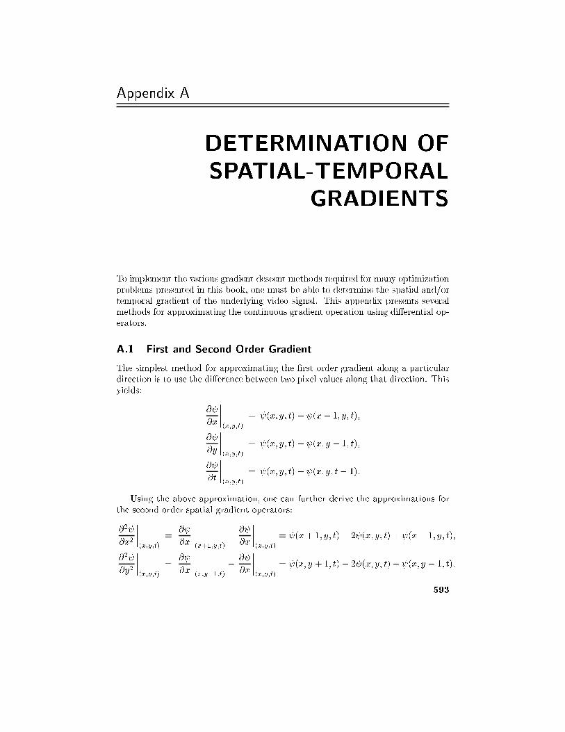
Appendix A
DETERMINATION OF
SPATIAL-TEMPORAL
GRADIENTS
To implement the various gradient descent methods required for many optimization
problems presented in this book, one must be able to determine the spatial and/or
temporal gradient of the underlying video signal. This appendix presents several
methods for approximating the continuous gradient operation using di�erential op-
erators.
A.1 First and Second Order Gradient
The simplest method for approximating the �rst order gradient along a particular
direction is to use the di�erence between two pixel values along that direction. This
yields:
@
@x
����(x;y;t)
= (x; y; t)� (x� 1; y; t);
@
@y
����(x;y;t)
= (x; y; t)� (x; y � 1; t);
@
@t
����(x;y;t)
= (x; y; t)� (x; y; t� 1):
Using the above approximation, one can further derive the approximations for
the second order spatial gradient operators:
@2
@x2
����(x;y;t)
=@
@x
����(x+1;y;t)
�
@
@x
����(x;y;t)
= (x+ 1; y; t)� 2 (x; y; t) + (x � 1; y; t);
@2
@y2
����(x;y;t)
=@
@x
����(x;y+1;t)
�
@
@x
����(x;y;t)
= (x; y + 1; t)� 2 (x; y; t) + (x; y � 1; t);
593
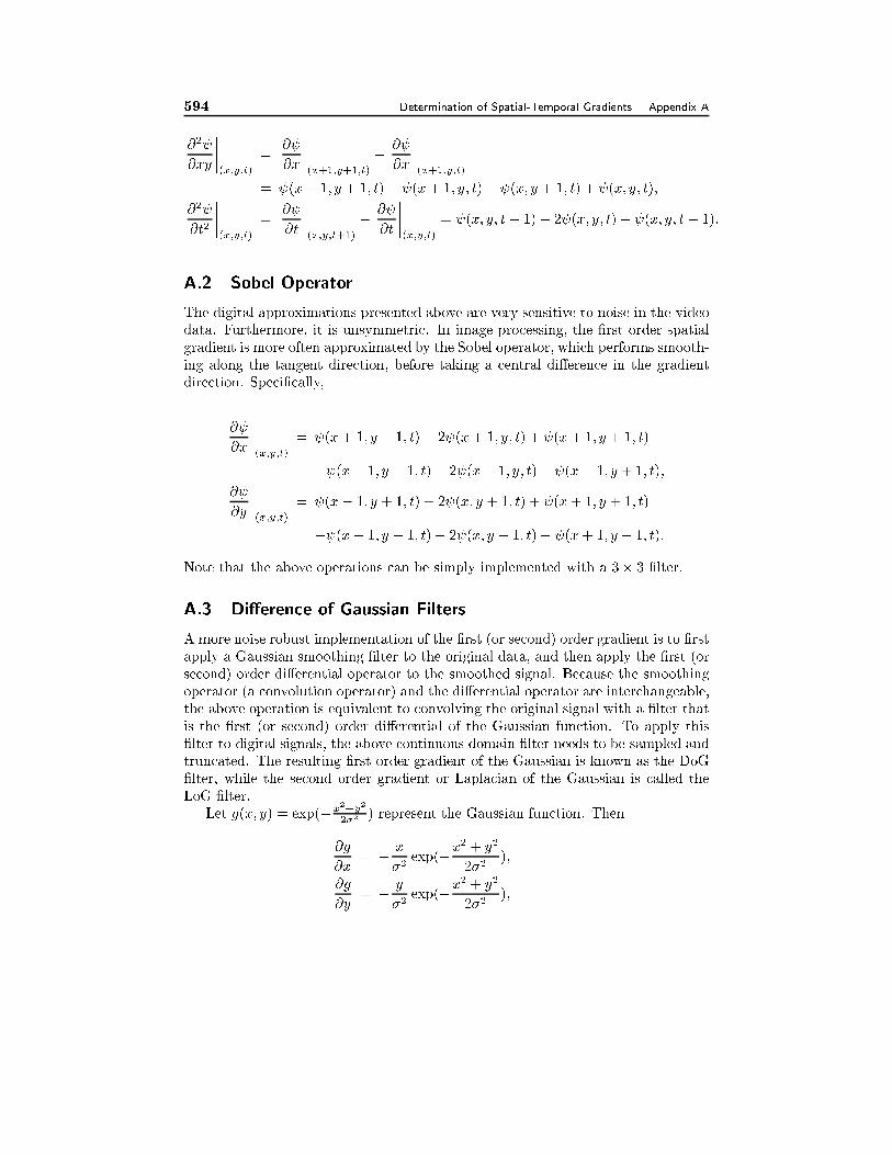
594 Determination of Spatial-Temporal Gradients Appendix A
@2
@xy
����(x;y;t)
=@
@x
����(x+1;y+1;t)
�
@
@x
����(x+1;y;t)
= (x+ 1; y + 1; t)� (x+ 1; y; t)� (x; y + 1; t) + (x; y; t);
@2
@t2
����(x;y;t)
=@
@t
����(x;y;t+1)
�
@
@t
����(x;y;t)
= (x; y; t+ 1)� 2 (x; y; t) + (x; y; t� 1):
A.2 Sobel Operator
The digital approximations presented above are very sensitive to noise in the video
data. Furthermore, it is unsymmetric. In image processing, the �rst order spatial
gradient is more often approximated by the Sobel operator, which performs smooth-
ing along the tangent direction, before taking a central di�erence in the gradient
direction. Speci�cally,
@
@x
����(x;y;t)
= (x+ 1; y � 1; t) + 2 (x+ 1; y; t) + (x+ 1; y + 1; t)
� (x� 1; y � 1; t)� 2 (x� 1; y; t)� (x� 1; y + 1; t);
@
@y
����(x;y;t)
= (x� 1; y + 1; t) + 2 (x; y + 1; t) + (x+ 1; y + 1; t)
� (x� 1; y � 1; t)� 2 (x; y � 1; t)� (x+ 1; y � 1; t):
Note that the above operations can be simply implemented with a 3� 3 �lter.
A.3 Di�erence of Gaussian Filters
A more noise robust implementation of the �rst (or second) order gradient is to �rst
apply a Gaussian smoothing �lter to the original data, and then apply the �rst (or
second) order di�erential operator to the smoothed signal. Because the smoothing
operator (a convolution operator) and the di�erential operator are interchangeable,
the above operation is equivalent to convolving the original signal with a �lter that
is the �rst (or second) order di�erential of the Gaussian function. To apply this
�lter to digital signals, the above continuous domain �lter needs to be sampled and
truncated. The resulting �rst order gradient of the Gaussian is known as the DoG
�lter, while the second order gradient or Laplacian of the Gaussian is called the
LoG �lter.
Let g(x; y) = exp(�x2+y
2
2�2 ) represent the Gaussian function. Then
@g
@x= �
x
�2exp(�
x2 + y2
2�2);
@g
@y= �
y
�2exp(�
x2 + y2
2�2);
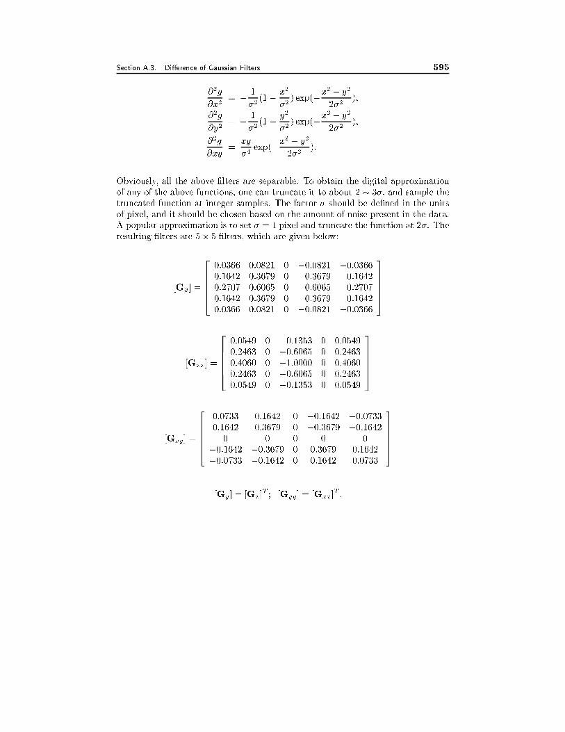
Section A.3. Di�erence of Gaussian Filters 595
@2g
@x2= �
1
�2(1�
x2
�2) exp(�
x2 + y2
2�2);
@2g
@y2= �
1
�2(1�
y2
�2) exp(�
x2 + y2
2�2);
@2g
@xy=
xy
�4exp(�
x2 + y2
2�2):
Obviously, all the above �lters are separable. To obtain the digital approximation
of any of the above functions, one can truncate it to about 2 � 3�, and sample the
truncated function at integer samples. The factor � should be de�ned in the units
of pixel, and it should be chosen based on the amount of noise present in the data.
A popular approximation is to set � = 1 pixel and truncate the function at 2�. The
resulting �lters are 5� 5 �lters, which are given below:
[Gx] =
266664
0:0366 0:0821 0 �0:0821 �0:0366
0:1642 0:3679 0 �0:3679 �0:1642
0:2707 0:6065 0 �0:6065 �0:2707
0:1642 0:3679 0 �0:3679 �0:1642
0:0366 0:0821 0 �0:0821 �0:0366
377775
[Gxx] =
266664
0:0549 0 �0:1353 0 0:0549
0:2463 0 �0:6065 0 0:2463
0:4060 0 �1:0000 0 0:4060
0:2463 0 �0:6065 0 0:2463
0:0549 0 �0:1353 0 0:0549
377775
[Gxy] =
266664
0:0733 0:1642 0 �0:1642 �0:0733
0:1642 0:3679 0 �0:3679 �0:1642
0 0 0 0 0
�0:1642 �0:3679 0 0:3679 0:1642
�0:0733 �0:1642 0 0:1642 0:0733
377775
[Gy] = [Gx]T ; [Gyy] = [Gxx]
T :
Appendix B
GRADIENT DESCENT
METHODS
In this appendix, we review some basic gradient descent methods for minimizing
an objective function. We will consider the general case when the function is mul-
tivariable with dimension K.
Let J(x) represent the objective function, where x = [x1; x2; : : : ; xk]T is a K-
dimensional vector. Gradient descent methods are iterative methods for determin-
ing the point x� that achieves the minimum of J(x).
B.1 First Order Gradient Descent Method
Let xl represent the solution at the l-th iteration. The �rst order gradient descent
method updates the solution proportional to the �rst order gradient of the objective
function, i.e.,
xl+1 = x
l� �
@J
@x
����xl
: (B.1.1)
The rationale behind the �rst order gradient descent method is that @J
@xrepresents
the direction along which the function J(x) increases most rapidly, and conse-
quently, �@J
@xis the direction along which J(x) decreases the fastest.
The constant � is known as the step-size. It has to be chosen properly to
guarantee the convergence of the above iteration process to the desired minimum
x�. If � is too large, the solution may oscillate around x
�; whereas if � is too
small, it may take too many iterations to converge. Obviously, if the function J(x)
has multiple local minima, then the solution upon convergence will be the local
minimum that is closest to the initial solution. Therefore, it is extremely important
to select an appropriate initial solution. In order to obtain the global minimum, one
can also start with several di�erent initial solutions that are suÆciently apart, and
run the above iteration scheme starting from each initial solution. By comparing
the function values at all the local minima obtained from di�erent initial solutions,
one can identify the one with the minimum value. However, there is no guarantee
596
Section B.2. Steepest Descent Method 597
that this will be the global minimum. A more sophisticated approach is simulated
annealing, which allows the iteration process to jump out of the local minima [1].
B.2 Steepest Descent Method
In the previous method, the step-size � is set to a small constant. To speed up
the convergence, one can also vary � at each new iteration, so that the maximum
reduction of J(x) is achieved. This is possible, because for �xed xl and @J
@x
��xl, the
new function value J(xl+1) is a scalar function of �. A numerical search method
can be used to determine the optimal step-size at each iteration. The �rst order
gradient descent method that uses such a variable step-size is known as the steepest
descent method. This method will converge in fewer iterations than the method
using a constant step-size, but each iteration will take more time to determine the
optimal step-size.
B.3 Newton's Method
The necessary condition for a function to achieve a local minimum is that its gradient
at that point is zero. Given a previous solution xl at which the gradient is not yet
zero, one way to determine the update is by requiring the gradient at the updated
position be zero, i.e.,
@J
@x
����xl+�x
= 0: (B.3.1)
Using Taylor's expansion for the above gradient function for up to the �rst term,
we obtain
@J
@x
����xl
+ [H(xl)]�x = 0; (B.3.2)
where
[H(x)] =@2J
@x2
����x
=
26664
@2J
@x1@x1
@2J
@x1@x2� � �
@2J
@x1@xK
@2J
@x2@x1
@2J
@x2@x2� � �
@2J
@x2@xK
� � � � � � � � � � � �
@2J
@xK@x1
@2J
@xK@x2� � �
@2J
@xK@xK
37775
is the second order derivative of J(x), known as the Hessian matrix. Solving
Eq. (B.3.2), we obtain
�x = � [H(xl)]�1 @J
@x
����xl
;
or
xl+1 = x
l� [H(xl)]
�1 @J
@x
����xl
:
598 Gradient Descent Methods Appendix B
The above iterative algorithm is known as the Newton method, which requires
the second order derivative, in addition to the �rst order derivative. The Newton
method can converge much faster, but each iteration requires signi�cantly more
calculation, and the algorithm is not guaranteed to converge. The use of the second
order derivative also makes this algorithm more prone to noise and numerical errors.
In reality, the following update is more often used
xl+1 = x
l� � [H(xl)]
�1 @J
@x
����xl
; (B.3.3)
where the step-size � is a constant smaller than 1, which needs to be chosen prop-
erly to reach a good compromise between guaranteeing the convergence and the
convergence rate.
B.4 Newton-Ralphson Method
When the objective function is a sum of squared errors, i.e.,
J(x) =1
2
Xk
e2k(x); (B.4.1)
we have@J
@x=X @ek
@xek(x); (B.4.2)
and
[H] =@2J
@x2=X @ek
@x
�@ek
@x
�T
+@2ek
@x2ek(x) �
X @ek
@x
�@ek
@x
�T
: (B.4.3)
The last approximation is obtained by assuming the term with the second order
derivative is signi�cantly smaller than that with the �rst order derivative only.
Using the above approximation in Eq. (B.3.3) yields the Newton-Ralphson method.
Because almost all the error minimization problems encountered in practice uses
a sum of error squares as an objective function, the Newton-Ralphson method is
widely used.
B.5 Bibliography
[1] P. J. M. Van Laarhoven and E. H. Aarts. Simulated Annealing: Theory and
Applications. Reidel, Dordrecht, Holland, 1987.
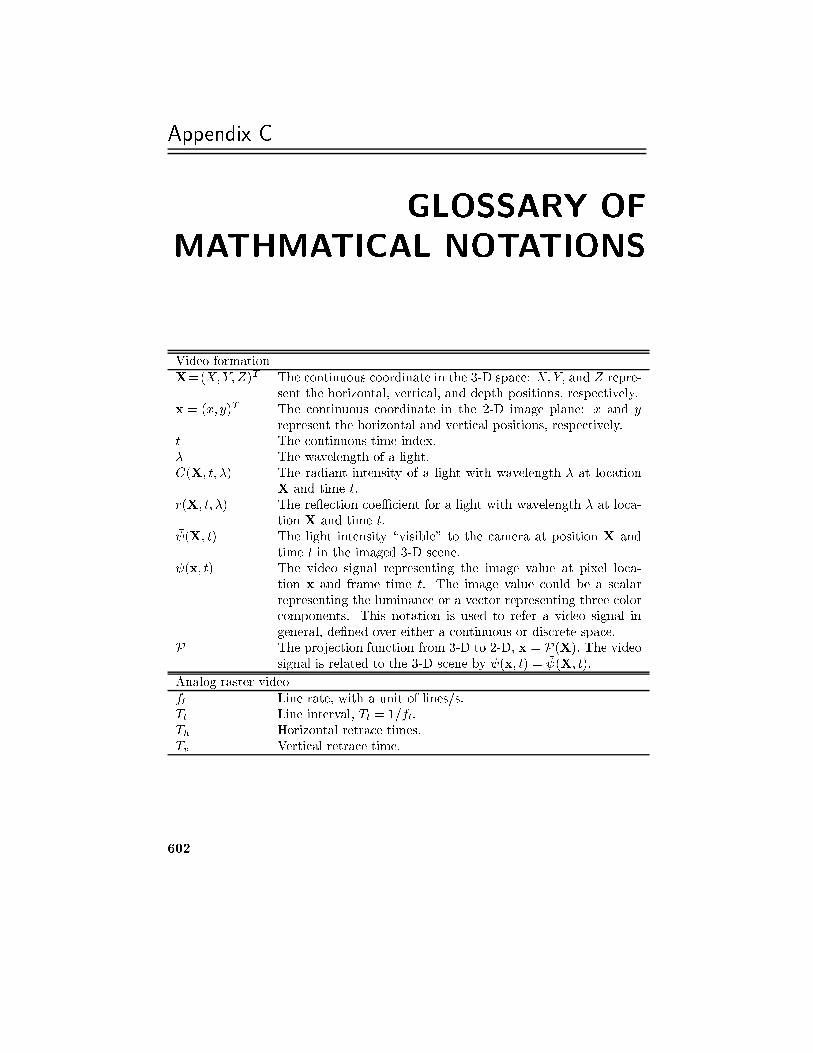
Appendix C
GLOSSARY OF
MATHMATICAL NOTATIONS
Video formation
X=(X;Y; Z)T The continuous coordinate in the 3-D space: X;Y; and Z repre-
sent the horizontal, vertical, and depth positions, respectively.
x = (x; y)T The continuous coordinate in the 2-D image plane: x and y
represent the horizontal and vertical positions, respectively.
t The continuous time index.
� The wavelength of a light.
C(X; t; �) The radiant intensity of a light with wavelength � at location
X and time t.
r(X; t; �) The re ection coeÆcient for a light with wavelength � at loca-
tion X and time t.� (X; t) The light intensity \visible" to the camera at position X and
time t in the imaged 3-D scene.
(x; t) The video signal representing the image value at pixel loca-
tion x and frame time t. The image value could be a scalar
representing the luminance or a vector representing three color
components. This notation is used to refer a video signal in
general, de�ned over either a continuous or discrete space.
P The projection function from 3-D to 2-D, x = P(X): The video
signal is related to the 3-D scene by (x; t) = � (X; t):
Analog raster video
fl Line rate, with a unit of lines/s.
Tl Line interval, Tl = 1=fl.
Th Horizontal retrace times.
Tv Vertical retrace time.
602
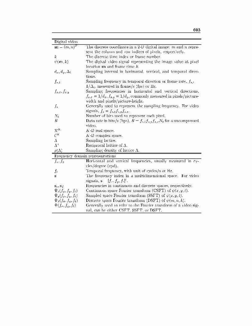
603
Digital video
m = (m;n)T The discrete coordinate in a 2-D digital image: m and n repre-
sent the column and row indices of pixels, respectively.
k The discrete time index or frame number.
(m; k) The digital video signal representing the image value at pixel
location m and frame time k.
dx; dy;�t Sampling interval in horizontal, vertical, and temporal direc-
tions.
fs;t Sampling frequency in temporal direction or frame rate, fs;t =
1=�t, measured in frame/s (fps) or Hz.
fs;x; fs;y Sampling frequencies in horizontal and vertical directions,
fs;x = 1=dx; fs;y = 1=dy, commonly measured in pixels/picture-
width and pixels/picture-height.
fs Generally used to represent the sampling frequency. For video
signals, fs = fs;tfs;yfs;x:
Nb Number of bits used to represent each pixel.
R Data rate in bits/s (bps), R = fs;tfs;yfs;xNb for a uncompressed
video.
RK K-D real space.
CK K-D complex space.
� Sampling lattice.
�� Reciprocal lattice of �:
�(�) Sampling density of lattice �:
Frequency domain representations
fx; fy Horizontal and vertical frequencies, usually measured in cy-
cles/degree (cpd).
ft Temporal frequency, with unit of cycles/s or Hz.
s The frequency index in a multidimensional space. For video
signals, s = [fx; fy; ft]t:
sc; sd Frequencies in continuous and discrete spaces, respectively.
c(fx; fy; ft) Continuous space Fourier transform (CSFT) of (x; y; t):
s(fx; fy; ft) Sampled space Fourier transform (SSFT) of (x; y; t):
d(fx; fy; ft) Discrete space Fourier transform (DSFT) of (m;n; k):
(fx; fy; ft) Generally used to refer to the Fourier transform of a video sig-
nal, can be either CSFT, SSFT, or DSFT.
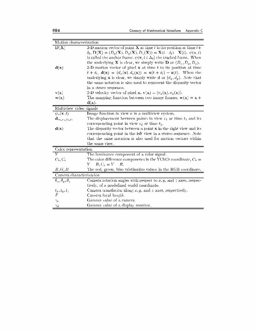
604 Glossary of Mathmatical Notations Appendix C
Motion characterization
D(X) 3-D motion vector of pointX at time t to its position at time t+
Æt, D(X) = (Dx(X); Dy(X); Dz(X)) = X(t+Æt)�X(t). (x; t)
is called the anchor frame, (x; t+�t) the tracked frame. When
the underlying X is clear, we simply write D or (Dx; Dy; Dz).
d(x) 2-D motion vector of pixel x at time t to its position at time
t + Æt, d(x) = (dx(x); dy(x)) = x(t + Æt) � x(t). When the
underlying x is clear, we simply write d or (dx; dy). Note that
the same notation is also used to represent the disparity vector
in a stereo sequence.
v(x) 2-D velocity vector of pixel x, v(x) = (vx(x); vy(x)).
w(x) The mapping function between two image frames, w(x) = x+
d(x):
Multiview video signals
v(x; t) Image function in view v in a multiview system.
dv1;v2;t1;t2 The displacement between points in view v1 at time t1 and its
corresponding point in view v2 at time t2:
d(x) The disparity vector between a point x in the right view and its
corresponding point in the left view in a stereo sequence. Note
that the same notation is also used for motion vectors within
the same view.
Color representation
Y The luminance component of a color signal.
Cb; Cr The color di�erence components in the YCbCr coordinate, Cb =
Y �B;Cr = Y � R:
R;G;B The red, green, blue tristimulus values in the RGB coordinate.
Camera characterization
�x; �y; �z Camera rotation angles with respect to x; y; and z axes, respec-
tively, of a prede�ned world coordinate.
tx; ty; tz Camera translation along x; y; and z axes, respectively.
F Camera focal length.
c Gamma value of a camera.
d Gamma value of a display monitor.
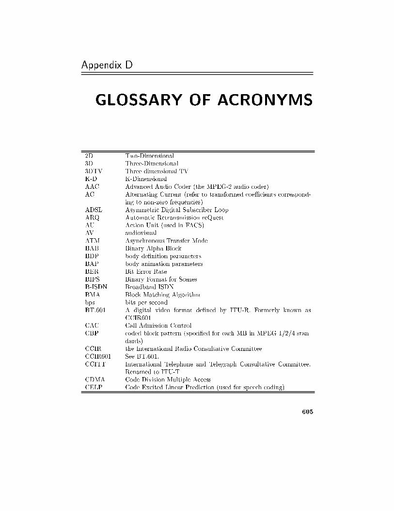
Appendix D
GLOSSARY OF ACRONYMS
2D Two-Dimensional
3D Three-Dimensional
3DTV Three-dimensional TV
K-D K-Dimensional
AAC Advanced Audio Coder (the MPEG-2 audio coder)
AC Alternating Current (refer to transformed coeÆcients correspond-
ing to non-zero frequencies)
ADSL Asymmetric Digital Subscriber Loop
ARQ Automatic Retransmission reQuest
AU Action Unit (used in FACS)
AV audiovisual
ATM Asynchronous Transfer Mode
BAB Binary Alpha Block
BDP body de�nition parameters
BAP body animation parameters
BER Bit Error Rate
BIFS Binary Format for Scenes
B-ISDN Broadband ISDN
BMA Block Matching Algorithm
bps bits per second
BT.601 A digital video format de�ned by ITU-R. Formerly known as
CCIR601
CAC Call Admission Control
CBP coded block pattern (speci�ed for each MB in MPEG-1/2/4 stan-
dards)
CCIR the International Radio Consultative Committee
CCIR601 See BT.601.
CCITT International Telephone and Telegraph Consultative Committee.
Renamed to ITU-T
CDMA Code Division Multiple Access
CELP Code Excited Linear Prediction (used for speech coding)
605
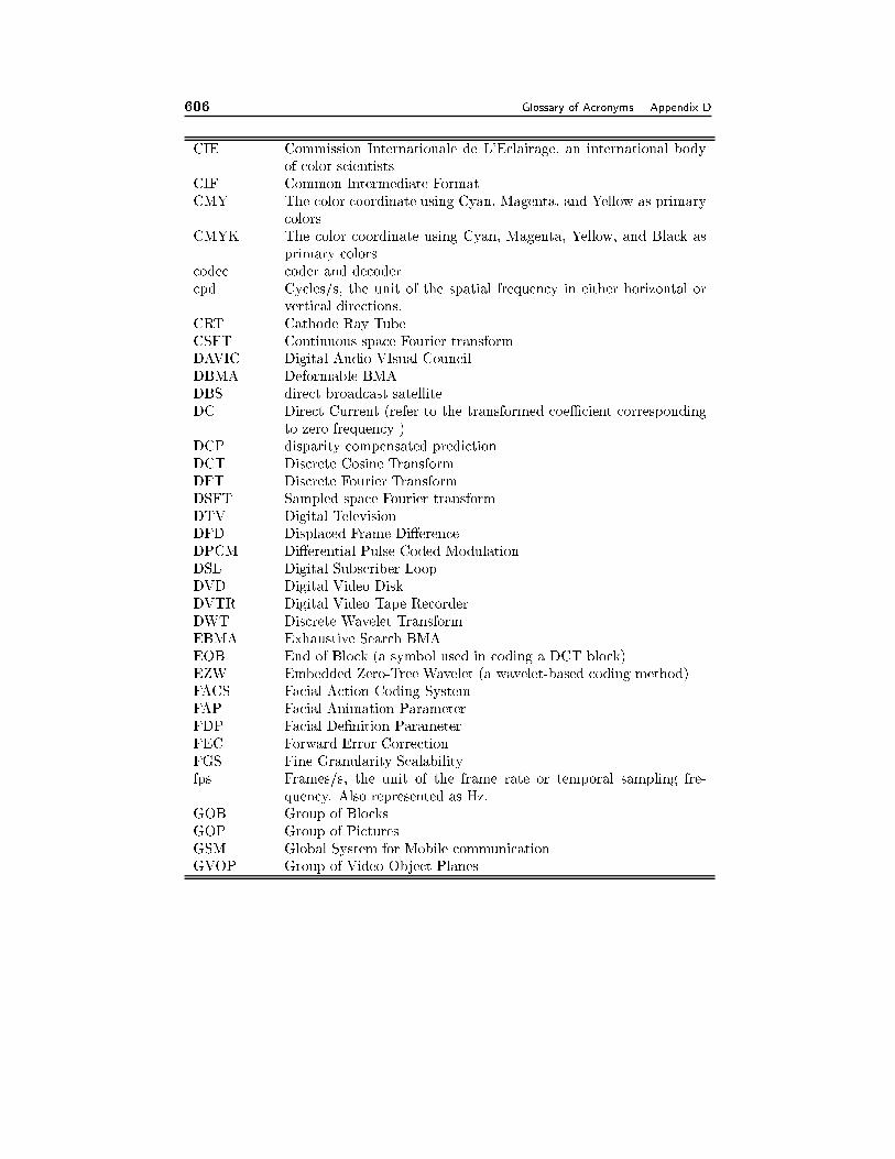
606 Glossary of Acronyms Appendix D
CIE Commission Internationale de L'Eclairage, an international body
of color scientists
CIF Common Intermediate Format
CMY The color coordinate using Cyan, Magenta, and Yellow as primary
colors
CMYK The color coordinate using Cyan, Magenta, Yellow, and Black as
primary colors
codec coder and decoder
cpd Cycles/s, the unit of the spatial frequency in either horizontal or
vertical directions.
CRT Cathode Ray Tube
CSFT Continuous space Fourier transform
DAVIC Digital Audio VIsual Council
DBMA Deformable BMA
DBS direct broadcast satellite
DC Direct Current (refer to the transformed coeÆcient corresponding
to zero frequency )
DCP disparity compensated prediction
DCT Discrete Cosine Transform
DFT Discrete Fourier Transform
DSFT Sampled space Fourier transform
DTV Digital Television
DFD Displaced Frame Di�erence
DPCM Di�erential Pulse Coded Modulation
DSL Digital Subscriber Loop
DVD Digital Video Disk
DVTR Digital Video Tape Recorder
DWT Discrete Wavelet Transform
EBMA Exhaustive Search BMA
EOB End of Block (a symbol used in coding a DCT block)
EZW Embedded Zero-Tree Wavelet (a wavelet-based coding method)
FACS Facial Action Coding System
FAP Facial Animation Parameter
FDP Facial De�nition Parameter
FEC Forward Error Correction
FGS Fine Granularity Scalability
fps Frames/s, the unit of the frame rate or temporal sampling fre-
quency. Also represented as Hz.
GOB Group of Blocks
GOP Group of Pictures
GSM Global System for Mobile communication
GVOP Group of Video Object Planes
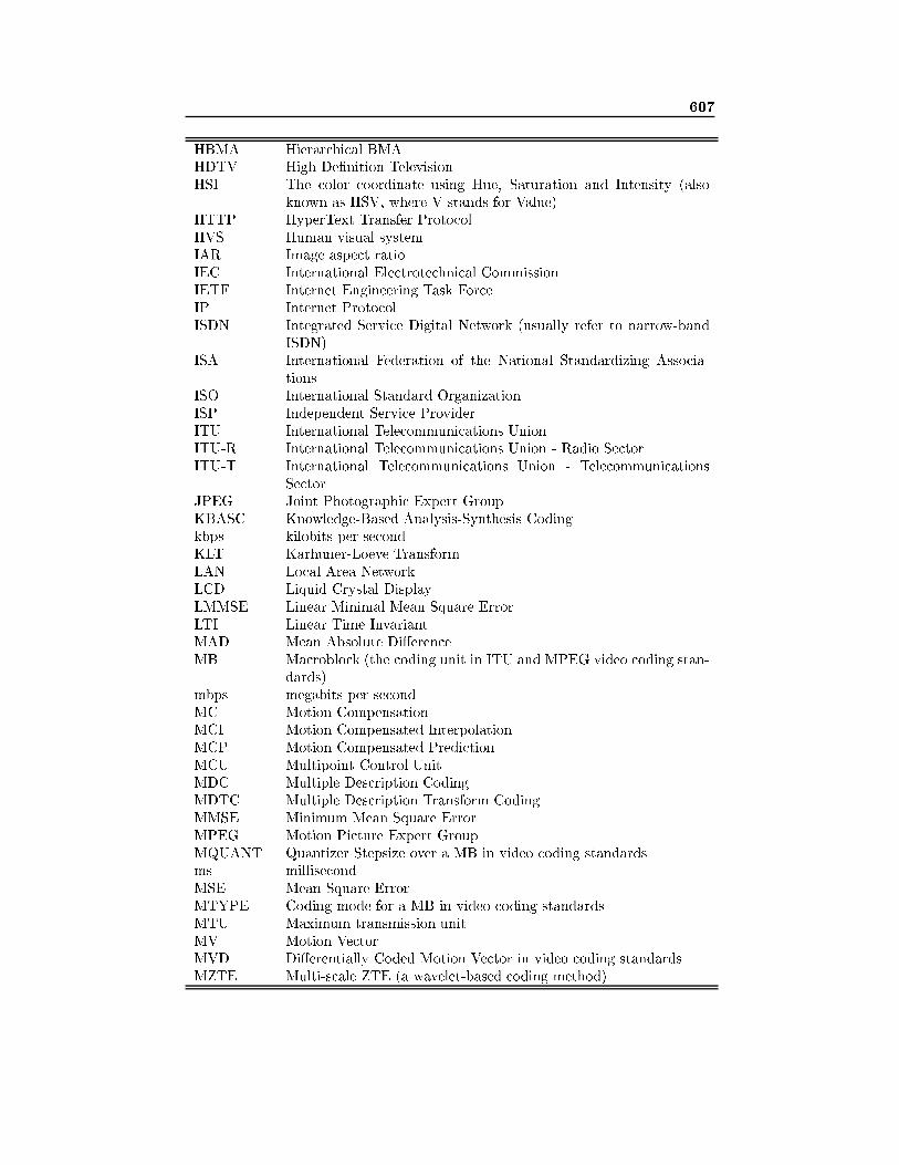
607
HBMA Hierarchical BMA
HDTV High De�nition Television
HSI The color coordinate using Hue, Saturation and Intensity (also
known as HSV, where V stands for Value)
HTTP HyperText Transfer Protocol
HVS Human visual system
IAR Image aspect ratio
IEC International Electrotechnical Commission
IETF Internet Engineering Task Force
IP Internet Protocol
ISDN Integrated Service Digital Network (usually refer to narrow-band
ISDN)
ISA International Federation of the National Standardizing Associa-
tions
ISO International Standard Organization
ISP Independent Service Provider
ITU International Telecommunications Union
ITU-R International Telecommunications Union - Radio Sector
ITU-T International Telecommunications Union - Telecommunications
Sector
JPEG Joint Photographic Expert Group
KBASC Knowledge-Based Analysis-Synthesis Coding
kbps kilobits per second
KLT Karhuner-Loeve Transform
LAN Local Area Network
LCD Liquid Crystal Display
LMMSE Linear Minimal Mean Square Error
LTI Linear Time Invariant
MAD Mean Absolute Di�erence
MB Macroblock (the coding unit in ITU and MPEG video coding stan-
dards)
mbps megabits per second
MC Motion Compensation
MCI Motion Compensated Interpolation
MCP Motion Compensated Prediction
MCU Multipoint Control Unit
MDC Multiple Description Coding
MDTC Multiple Description Transform Coding
MMSE Minimum Mean Square Error
MPEG Motion Picture Expert Group
MQUANT Quantizer Stepsize over a MB in video coding standards
ms millisecond
MSE Mean Square Error
MTYPE Coding mode for a MB in video coding standards
MTU Maximum transmission unit
MV Motion Vector
MVD Di�erentially Coded Motion Vector in video coding standards
MZTE Multi-scale ZTE (a wavelet-based coding method)
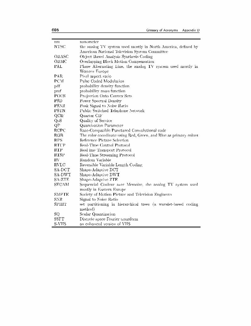
608 Glossary of Acronyms Appendix D
nm nanometer
NTSC the analog TV system used mostly in North America, de�ned by
American National Television System Committee
OBASC Object-Based Analysis-Synthesis Coding
OBMC Overlapping Block Motion Compensation
PAL Phase Alternating Line, the analog TV system used mostly in
Western Europe
PAR Pixel aspect ratio
PCM Pulse Coded Modulation
pdf probability density function
pmf probability mass function
POCS Projection Onto Convex Sets
PSD Power Spectral Density
PSNR Peak Signal to Noise Ratio
PSTN Public Switched Telephone Network
QCIF Quarter CIF
QoS Quality of Service
QP Quantization Parameter
RCPC Rate-Compatible Punctured Convolutional code
RGB The color coordinate using Red, Green, and Blue as primary colors
RPS Reference Picture Selection
RTCP Real-Time Control Protocol
RTP Real-ime Transport Protocol
RTSP Real-Time Streaming Protocol
RV Random Variable
RVLC Reversible Variable Length Coding
SA-DCT Shape-Adaptive DCT
SA-DWT Shape-Adaptive DWT
SA-ZTE Shape-Adaptive ZTE
SECAM Sequential Couleur avec Memoire, the analog TV system used
mostly in Eastern Europe
SMPTE Society of Motion Picture and Television Engineers
SNR Signal to Noise Ratio
SPIHT set partitioning in hierarchical trees (a wavelet-based coding
method)
SQ Scalar Quantization
SSFT Discrete space Fourier transform
S-VHS an enhanced version of VHS
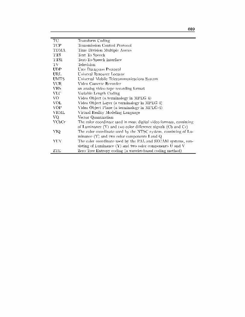
609
TC Transform Coding
TCP Transmission Control Protocol
TDMA Time Division Multiple Access
TTS Text-To-Speech
TTSI Text-To-Speech Interface
TV Television
UDP User Datagram Protocol
URL Univeral Resource Locator
UMTS Universal Mobile Telecommunications System
VCR Video Cassette Recorder
VHS an analog video tape recording format
VLC Variable Length Coding
VO Video Object (a terminalogy in MPEG-4)
VOL Video Object Layer (a terminalogy in MPEG-4)
VOP Video Object Plane (a terminalogy in MPEG-4)
VRML Virtual Reality Modeling Language
VQ Vector Quantization
YCbCr The color coordinate used in most digital video formats, consisting
of Luminance (Y) and two color di�erence signals (Cb and Cr)
YIQ The color coordinate used by the NTSC system, consisting of Lu-
minance (Y) and two color components I and Q
YUV The color coordinate used by the PAL and SECAM systems, con-
sisting of Luminance (Y) and two color components U and V
ZTE Zero Tree Entropy coding (a wavelet-based coding method)
Related Documents