VARIATIONAL KALMAN FILTERING ON PARALLEL COMPUTERS

Variational Kalman Filtering

on Parallel Computers

Harri Auvinen, Tuomo Kauranne and Heikki HaarioDepartment of Mathematics

Lappeenranta University of [email protected]

31 October 2006

Outline

⇒ Bene�ts of Kalman Filtering (KF)

⇒ Feasible Approximations to KF

⇒ The Structure of Variational Kalman Filter (VKF) Computations

⇒ Properties of the Variational Kalman Filter

⇒ Serial and Parallel Complexity of VKF

⇒ Computational Results with the Lorenz'95 Model

⇒ Conclusions

1

Bene�ts of Kalman Filtering (KF)

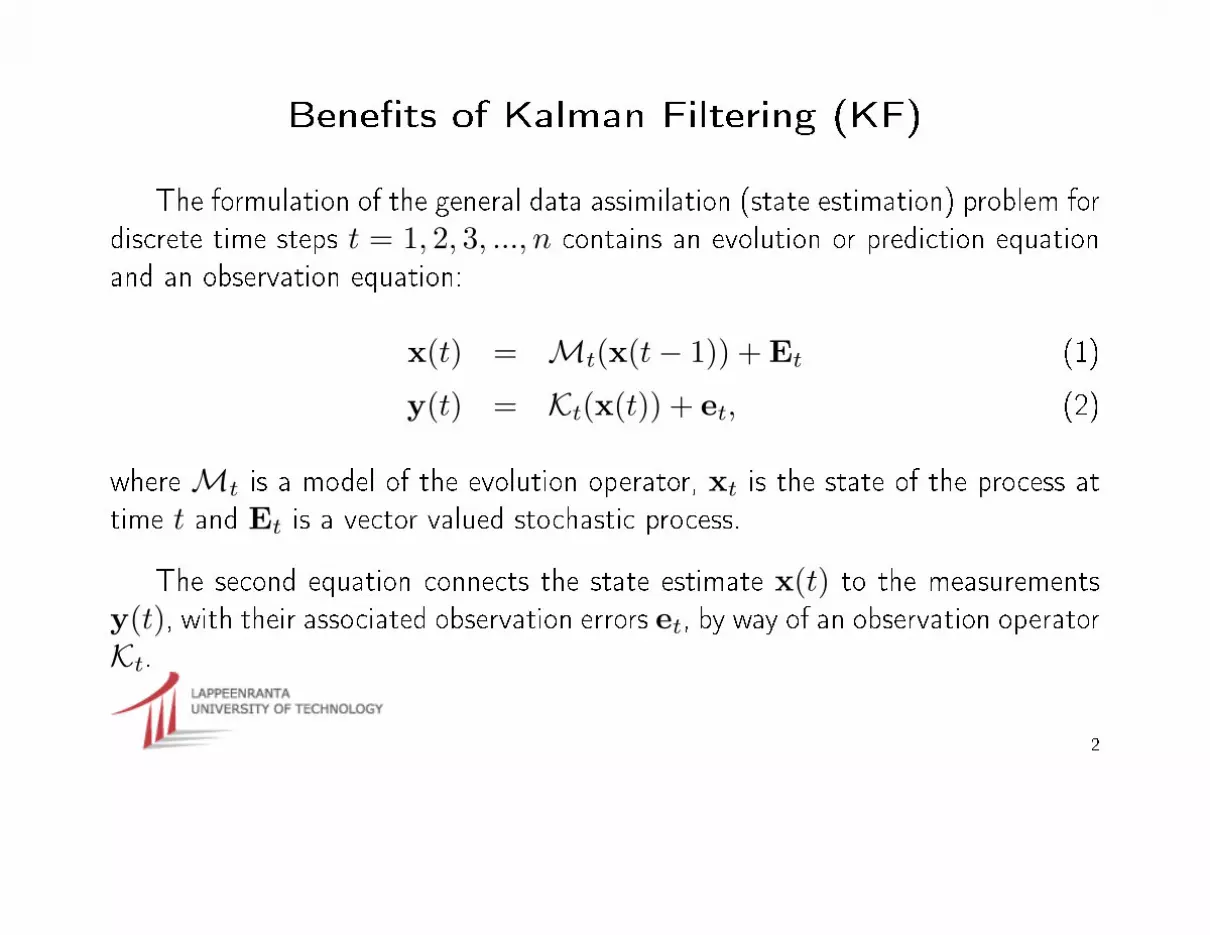
The formulation of the general data assimilation (state estimation) problem fordiscrete time steps t = 1, 2, 3, ..., n contains an evolution or prediction equationand an observation equation:

x(t) = Mt(x(t− 1)) + Et (1)

y(t) = Kt(x(t)) + et, (2)

whereMt is a model of the evolution operator, xt is the state of the process attime t and Et is a vector valued stochastic process.

The second equation connects the state estimate x(t) to the measurementsy(t), with their associated observation errors et, by way of an observation operatorKt.

2

Bene�ts of Kalman Filtering (KF)

⇒ The optimal linear estimator to the data assimilation problem is the ExtendedKalman Filter (EKF).

⇒ EKF can compensate for model bias

⇒ EKF analyses are discontinuous, but can be smoothed out afterwards

⇒ The analysis error covariance matrix can be used for assessing predictability

⇒ Its singular vectors can be used as initial perturbations to Ensemble Forecasting,if the time interval over which they have been computed is appropriate

3

Feasible Approximations to KF

⇒ EKF requires that in addition to evolving the model state with the nonlinearforecast model, all the columns of the analysis error covariance matrix beevolved back and forth in time, with the adjoint model and the tangent linearmodel in succession.

⇒ This is prohibitively expensive, and we must �nd feasible approximations toEKF.

4

Feasible Approximations to KF

⇒ 4D-Var is the special case of EKF where the model is perfect and the analysiserror covariance matrix is static

⇒ In Reduced Rank Kalman Filtering (RRKF), the covariance matrix is constantlyprojected onto a �xed low dimensional subspace and evolved only there

⇒ In Ensemble Kalman Filtering (EnKF), a set of random perturbations is evolvedto form a statistical sample of the span of the analysis error covariance matrix

5

Design Principles of the Variational Kalman Filter

(VKF)

⇒ VKF - like EKF - behaves like a continuous data assimilation method

⇒ It is robust against model error

⇒ It produces a good estimate to the analysis error covariance matrix

⇒ VKF is highly parallel

6

Kalman Filter algorithm (1/2)

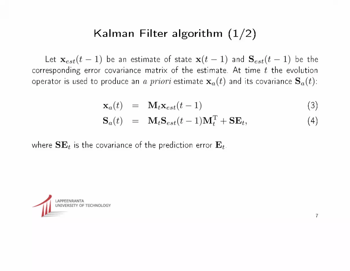
Let xest(t − 1) be an estimate of state x(t − 1) and Sest(t − 1) be thecorresponding error covariance matrix of the estimate. At time t the evolutionoperator is used to produce an a priori estimate xa(t) and its covariance Sa(t):

xa(t) = Mtxest(t− 1) (3)

Sa(t) = MtSest(t− 1)MTt + SEt, (4)

where SEt is the covariance of the prediction error Et.

7

Kalman Filter algorithm (2/2)

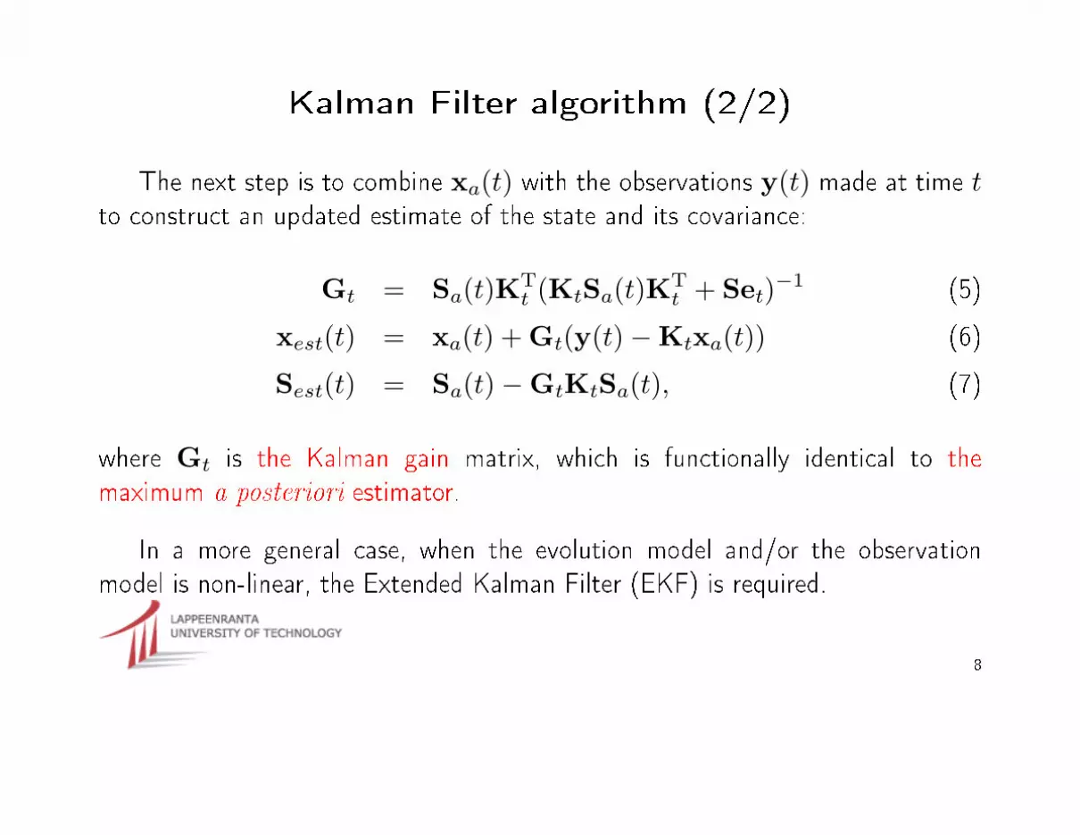
The next step is to combine xa(t) with the observations y(t) made at time tto construct an updated estimate of the state and its covariance:

Gt = Sa(t)KTt (KtSa(t)KT

t + Set)−1 (5)

xest(t) = xa(t) + Gt(y(t)−Ktxa(t)) (6)

Sest(t) = Sa(t)−GtKtSa(t), (7)

where Gt is the Kalman gain matrix, which is functionally identical to themaximum a posteriori estimator.

In a more general case, when the evolution model and/or the observationmodel is non-linear, the Extended Kalman Filter (EKF) is required.

8

Extended Kalman Filter algorithm (1/3)

The �lter uses the full non-linear evolution model equation (1) to produce ana priori estimate: xa(t) =Mt(xest(t− 1)) .

In order to obtain the corresponding covariance Sa(t) of the a priori

information, the prediction model is linearized about xest(t− 1):

Mt =∂Mt(xest(t− 1))

∂x(8)

Sa(t) = MtSest(t− 1)MTt + SEt. (9)

The linearization Mt of the modelMt in equation (8) is computed as thetangent linear model, from which the adjoint model MT

t is obtained as itstranspose.

9


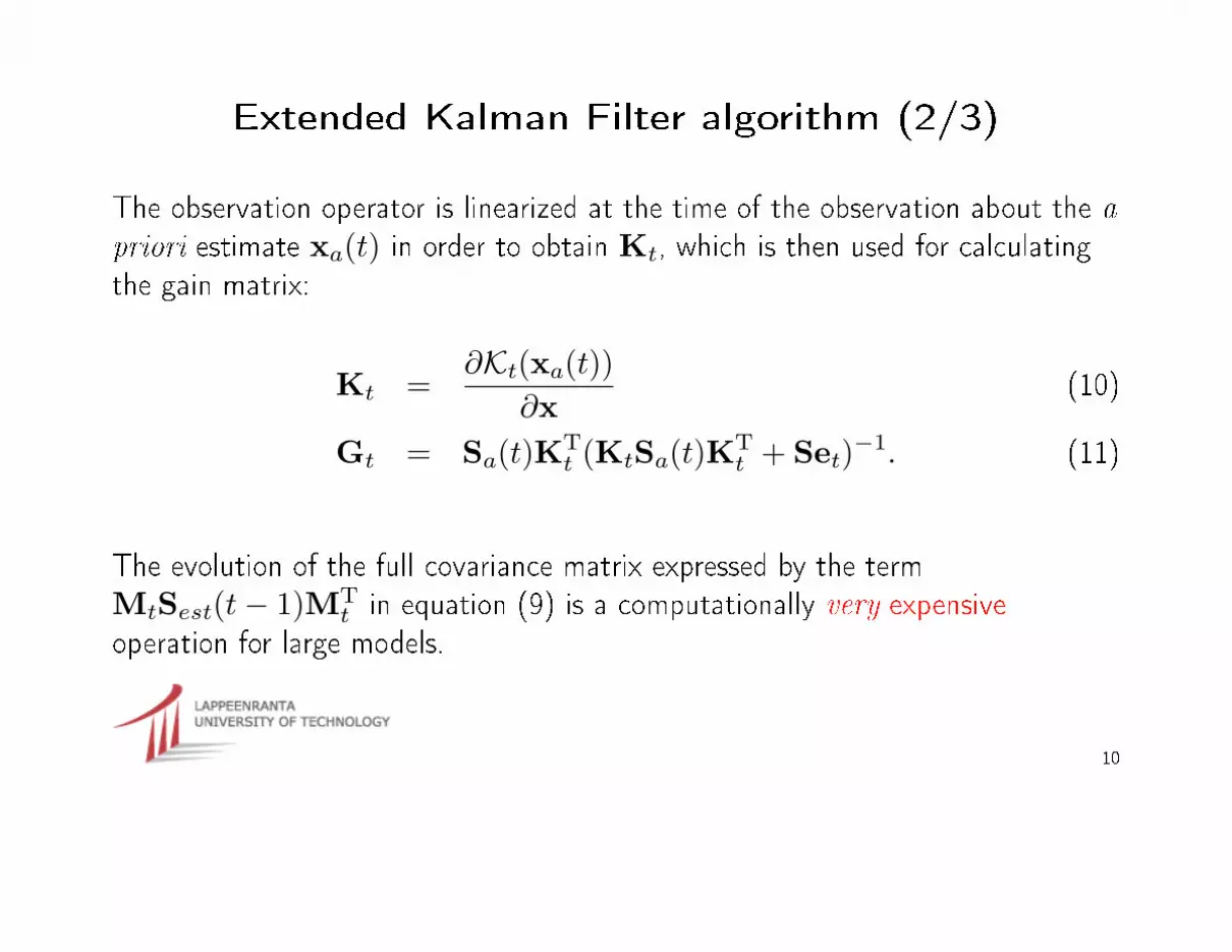
The observation operator is linearized at the time of the observation about the apriori estimate xa(t) in order to obtain Kt, which is then used for calculatingthe gain matrix:

Kt =∂Kt(xa(t))

∂x(10)

Gt = Sa(t)KTt (KtSa(t)KT

t + Set)−1. (11)

The evolution of the full covariance matrix expressed by the termMtSest(t− 1)MT

t in equation (9) is a computationally very expensiveoperation for large models.

10


After this, the full non-linear observation operator is used to update xa(t) andthis is then used to produce a current state estimate and the corresponding errorestimate:

xest(t) = xa(t) + Gt(y(t)−Kt(xa(t))). (12)

Sest(t) = Sa(t)−GtKtSa(t). (13)

If the linearization of the observation operator at xa(t) is not good enough toconstruct xest(t), it will be necessary to carry out some iterations of the lastfour equations.

11

Variational Kalman Filter algorithm (1/5)

The VKF method uses the full non-linear prediction equation (1) to construct ana priori estimate from the previous state estimate:

xa(t) =Mt(xest(t− 1)). (14)

The corresponding approximated covariance Sa(t) of the a priori information isavailable from the previous time step of VKF method.

In order to avoid the computation of the Kalman gain we perform a 3D-Varoptimization with a Kalman equivalent cost function. As the result of theoptimization, we get the state estimate xest(t) for the present time t.

12


The error estimate Sest(t) of the state estimate is obtained from the formula:

Sest(t) = 2(Hess(t))−1, (15)

where the inverse of the matrix Hess(t) can be approximated by using thesearch directions of the optimization process. These directions are used also bythe Quasi-Newton method used in the minimization for creating anapproximation to the Hessian of the cost function.

13


The estimate of the analysis error covariance is updated from the previousestimate using the Kalman formula

Sa(t) = Mt−1(Sest(t− 1) + SPt−1)MTt−1 + SEt, (16)

where SPt is a stochastic process representing the variance of the matrix valuedtruncation error incurred in approximating the analysis error covariance matrixSa(t) by the approximate inverse Hessian (Hess(t))−1 from the minimization.

We split Sest(t− 1) into a static background covariance B that represents thelong term mean of the covariance matrix and to a low rank transient component,kept in vector form, which is transformed by the adjoint and tangent linearmodels.

14


In practice, the inverse of the Hessian only is kept, and in vector form to boot.The required multiplications with the analysis error covariance matrix are carriedout with the Sherman-Morrison-Woodbury formula.

During the optimization another task is done: the full non-linear evolution modelequation (1) is used to transfer search directions to the next time step t + 1.These evolved search directions are then used to update the approximation of thepresent covariance Sa(t) in order to approximate Sa(t + 1).

The other vectors used to approximate Sa(t) should be transferred by thenonlinear evolution as well, if there is a long interval between observations. In ourcurrent experiments, it has proven su�cient just to use them as they stand andstill retain the useful qualities of VKF intact.

15


In order to maintain an upper limit on the rank of the Hessian approximation usedin the L-BFGS Quasi-Newton method, the updates are carried out by using thelimited memory Broyden-Fletcher-Goldfarb-Shannon (L-BFGS) update formulas.

After a 3D-Var optimization we have an updated covariance Sa(t) which is thenused to produce:

Sa(t + 1) = Sa(t) + SEt. (17)

At each iteration of the optimization method the evolved search directions andthe evolved gradients of J are stored and the approximation of the Sa(t) isupdated as the optimization method updates it's own approximation of theinverse Hessian (∇∇J)−1.

16

The Structure of VKF Computations

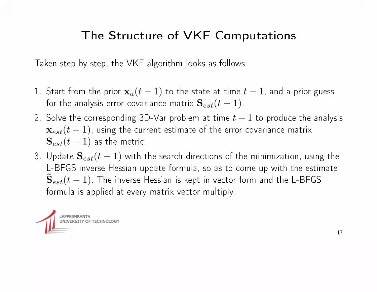
Taken step-by-step, the VKF algorithm looks as follows

1. Start from the prior xa(t− 1) to the state at time t− 1, and a prior guessfor the analysis error covariance matrix Sest(t− 1).

2. Solve the corresponding 3D-Var problem at time t− 1 to produce the analysisxest(t− 1), using the current estimate of the error covariance matrixSest(t− 1) as the metric

3. Update Sest(t− 1) with the search directions of the minimization, using theL-BFGS inverse Hessian update formula, so as to come up with the estimateSest(t− 1). The inverse Hessian is kept in vector form and the L-BFGSformula is applied at every matrix vector multiply.

17


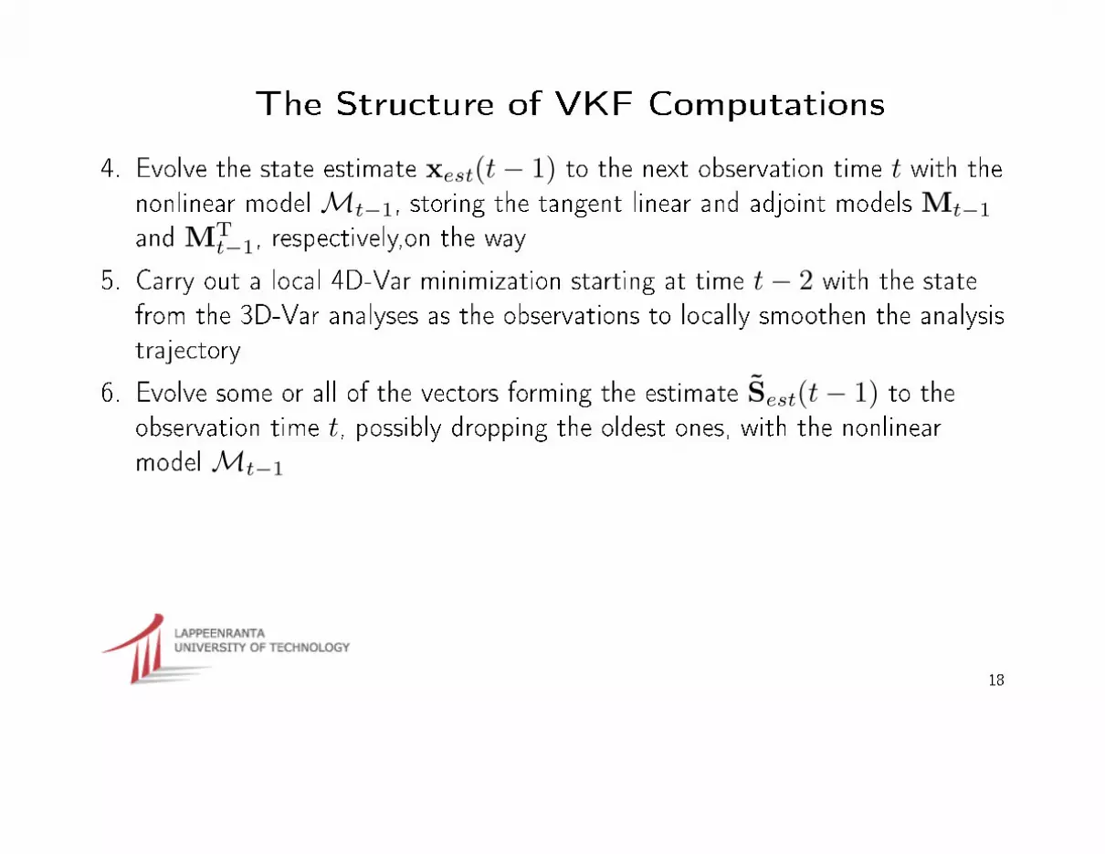
4. Evolve the state estimate xest(t− 1) to the next observation time t with thenonlinear modelMt−1, storing the tangent linear and adjoint models Mt−1

and MTt−1, respectively,on the way

5. Carry out a local 4D-Var minimization starting at time t− 2 with the statefrom the 3D-Var analyses as the observations to locally smoothen the analysistrajectory

6. Evolve some or all of the vectors forming the estimate Sest(t− 1) to theobservation time t, possibly dropping the oldest ones, with the nonlinearmodelMt−1

18


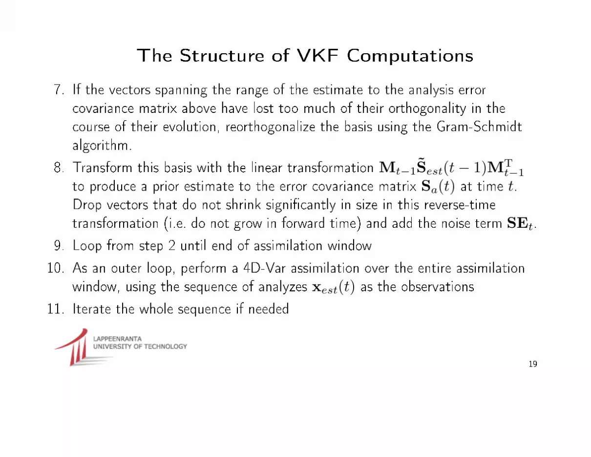
7. If the vectors spanning the range of the estimate to the analysis errorcovariance matrix above have lost too much of their orthogonality in thecourse of their evolution, reorthogonalize the basis using the Gram-Schmidtalgorithm.

8. Transform this basis with the linear transformation Mt−1Sest(t− 1)MTt−1

to produce a prior estimate to the error covariance matrix Sa(t) at time t.Drop vectors that do not shrink signi�cantly in size in this reverse-timetransformation (i.e. do not grow in forward time) and add the noise term SEt.

9. Loop from step 2 until end of assimilation window

10. As an outer loop, perform a 4D-Var assimilation over the entire assimilationwindow, using the sequence of analyzes xest(t) as the observations

11. Iterate the whole sequence if needed

19


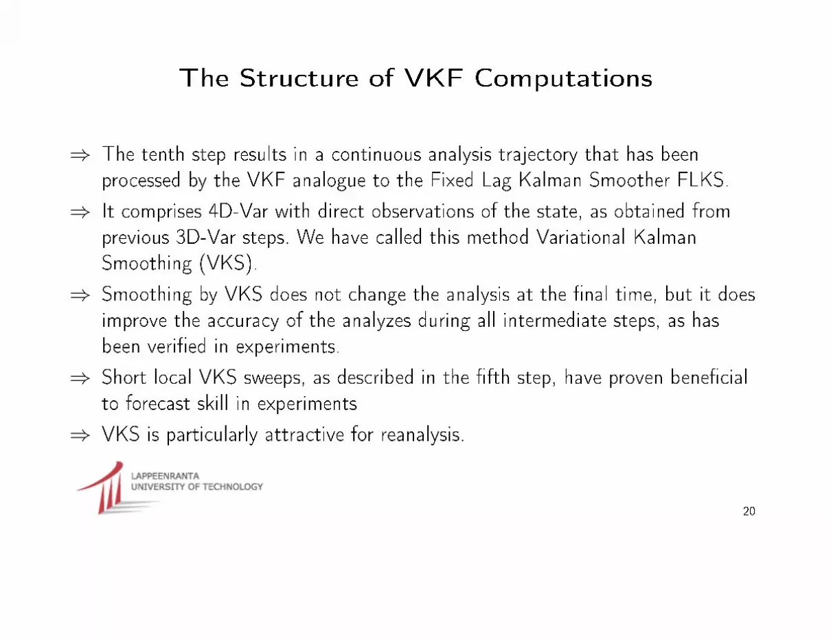
⇒ The tenth step results in a continuous analysis trajectory that has beenprocessed by the VKF analogue to the Fixed Lag Kalman Smoother FLKS.

⇒ It comprises 4D-Var with direct observations of the state, as obtained fromprevious 3D-Var steps. We have called this method Variational KalmanSmoothing (VKS).

⇒ Smoothing by VKS does not change the analysis at the �nal time, but it doesimprove the accuracy of the analyzes during all intermediate steps, as hasbeen veri�ed in experiments.

⇒ Short local VKS sweeps, as described in the �fth step, have proven bene�cialto forecast skill in experiments

⇒ VKS is particularly attractive for reanalysis.

20

The Serial Complexity of VKF Computations

⇒ Looking at the complexities and summing over all the steps, we see that thedominant serial cost in VKF consist of the advection of the covariance vectorsback and forth, of the 3D-Var steps, the local 4D-Var steps, and of the4D-Var minimization at the end.

⇒ Altogether, every vector of the inverse of the error covariance matrix storedrequires three model or adjoint model integrations (in fact, once with each ofthe three models: the nonlinear one, the tangent linear one and the adjointone).

⇒ If we were to keep the rank of the error covariance matrix at just the numberof most recent search directions, the overall complexity of the VKF algorithmwould amount just to two subsequent 4D-Var minimizations over the"one-and-a-half"assimilation window.

21

The Serial Complexity of VKF Computations

⇒ This is so, because the 3D-Var minimizations can be seen to be part of asingle model integration with the 4D-Var algorithm in any case, and because4D-Var requires as many model and adjoint model integrations as it takessteps to converge.

⇒ If it proves desirable to maintain a higher rank approximation to the errorcovariance matrix, the total serial complexity of VKF is multiplied by thisrank, divided by a typical number of steps needed by 4D-Var to converge.

⇒ An educated guess would put the total serial complexity of VKF at two to �vetimes the complexity of 4D-Var, and growing linearly with the resolution, justlike the complexity of 4D-Var does.

22

The Parallel Complexity of VKF Computations

Let us now turn our sights on the parallel computational complexity of VKF andreview parallelisation opportunities at each step

1. No computations yet

2. Standard 3D-Var at every observation time. No gain from parallelism.

3. Matrix update with a �xed number of vectors of the size of model resolution.Complexity is linear in spatial resolution and independent of the time step. Noeasy gains from parallelism.

4. A single model run to the next time step, with the standard tangent linearand adjoint coe�cient stores on the way. No parallelism.

5. A short 4D-Var minimization with identity as observation operator.

23

6. A number of forward model runs with a �xed number (a few, possibly a fewdozen) of independent initial states. All these are independent, and can becarried out in parallel.

7. Standard linear algebra with a �xed number of vectors of the size of modelresolution. Complexity is linear in spatial resolution and independent of thetime step. No parallelism.

8. A number of adjoint and subsequent tangent linear model runs, once backand forth for every vector, with a �xed number (a few, possibly a few dozen)of independent initial states, plus a sparse matrix vector product for each.Just as in step four, these can be fully parallelized, since we keep theapproximate Hessian in vector form.

9. The steps above are taken over the entire assimilation window, instead of justbetween subsequent observation times

10. Standard 4D-Var over the entire assimilation window

24


⇒ Many supercomputers in current operational weather forecasting centres, suchas the IBM Cluster at ECMWF, or the 70 T�ops Cray Hood just ordered byCSC to Finland, or the 100 Tera�ops Hood ordered by NERSC, have aclustered structure.

⇒ These parallel computers have dozens of Tera�ops of computing power, andthe operational weather models have been parallellized in a scalable fashion.

⇒ However, parallel supercomputers based on commodity processors have asigni�cant bottleneck in their inter-cluster communications.

⇒ Because of Amdahls's and Hockney's laws, this limits the bisection bandwidthof the machines so badly that operational models are often run within a singlecluster of processors only. (The Earth Simulator is a notable exception!)

25


⇒ VKF has an ideal structure to �t itself neatly onto such a parallel architecture,with potentially close to linear speedup. This follows from the independenceof the evolution steps of all the transient vectors used in approximating theanalysis error covariance matrix.

⇒ Looking at the parallel complexities of the individual steps, and summing overall the steps, we get a surprising result: the parallel complexity of VKF isequivalent to just three model runs and local VKS sweeps, apart from the�nal 4D-Var smoothing step.

⇒ Moreover, the last 4D-Var iteration does not change the analysis at the �naltime step. This means that if we are to launch the next forecast from it wecan postpone the 4D-Var to be carried out afterwards, outside the operationalcycle, for archival and reanalysis purposes.

26


⇒ We arrive therefore at a rather striking conclusion: the parallel complexity ofVKF in the operational cycle is just three model runs, one with each model:the nonlinear one, the adjoint one and the tangent linear one, and a single,rapidly converging simpli�ed 4D-Var.

⇒ Parallel complexity of VKF is also independent of the rank of the errorcovariance approximation, as long as this remains modest. If the covariancematrix is kept in vector form, all matrix vector products with it are fullyparallelisable.

⇒ VKF is therefore potentially faster than even the standard

4D-Var on a su�ciently powerful - yet realistic - parallel

computer.

27

Simulated assimilation results in Lorenz'95 case

We are very grateful to Mike Fisher and Martin Leutbecher of ECMWF forproviding us with their codes for the Lorenz'95 model and the weak constraint4D-Var and EKF data assimilation algorithms for it.

The assimilation results presented below are generated using the simplenon-linear model introduced by Lorenz[1] in 1995. The model is small andrepresents simpli�ed mid-latitude atmospheric dynamics of a single variable.

[1] E. N. Lorenz: Predictability: A problem partly solved. Proc. seminar onPredictability, Vol. 1, ECMWF, Reading, Berkshire, UK, 1-18, (1995).

[2] E. N. Lorenz and K. A. Emanuel: Optimal sites for supplementary weatherobservations: Simulations with a small model. J. Atmos. Sci., 55, 399-414,(1998).

28

Lorenz'95 model and parameters

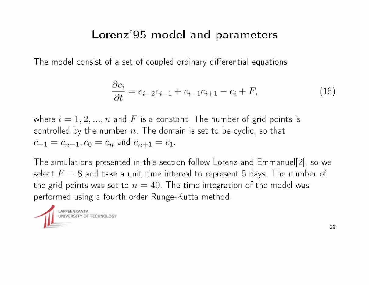
The model consist of a set of coupled ordinary di�erential equations

∂ci

∂t= ci−2ci−1 + ci−1ci+1 − ci + F, (18)

where i = 1, 2, ..., n and F is a constant. The number of grid points iscontrolled by the number n. The domain is set to be cyclic, so thatc−1 = cn−1, c0 = cn and cn+1 = c1.

The simulations presented in this section follow Lorenz and Emmanuel[2], so weselect F = 8 and take a unit time interval to represent 5 days. The number ofthe grid points was set to n = 40. The time integration of the model wasperformed using a fourth order Runge-Kutta method.

29

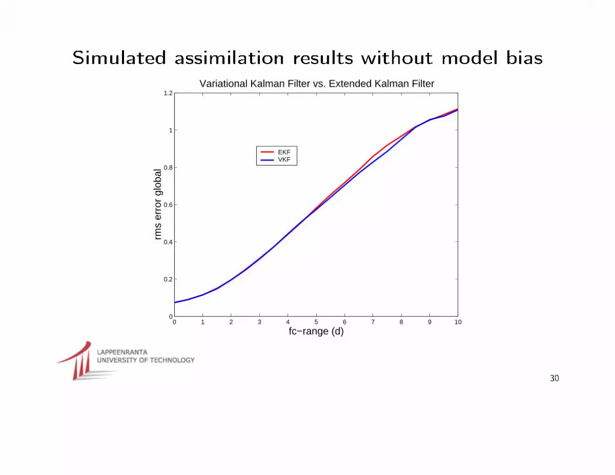
Simulated assimilation results without model bias

0 1 2 3 4 5 6 7 8 9 100

0.2

0.4

0.6

0.8

1

1.2Variational Kalman Filter vs. Extended Kalman Filter

fc−range (d)

rms

erro

r gl

obal

EKFVKF

30

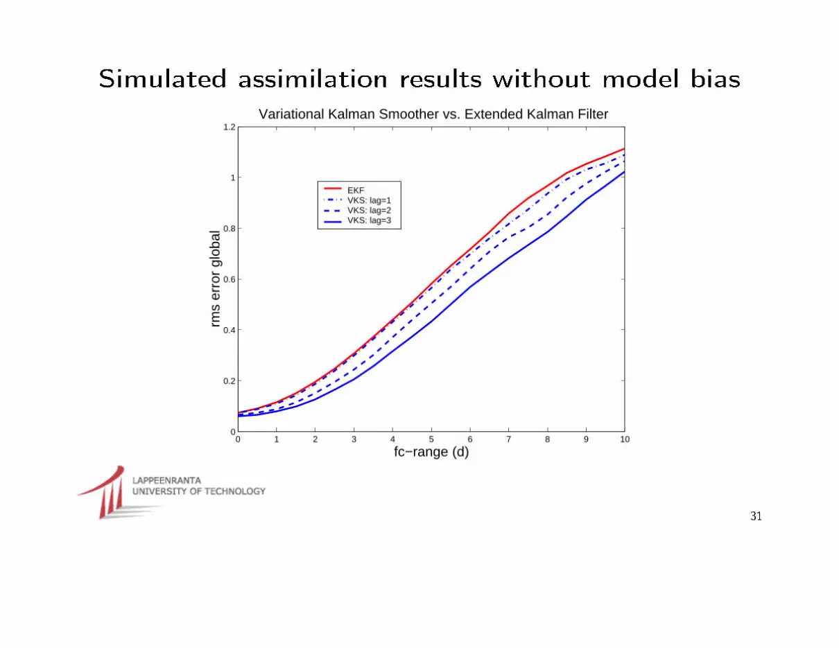
Simulated assimilation results without model bias

0 1 2 3 4 5 6 7 8 9 100

0.2

0.4

0.6

0.8

1

1.2Variational Kalman Smoother vs. Extended Kalman Filter

fc−range (d)

rms

erro

r gl

obal

EKF VKS: lag=1VKS: lag=2VKS: lag=3

31

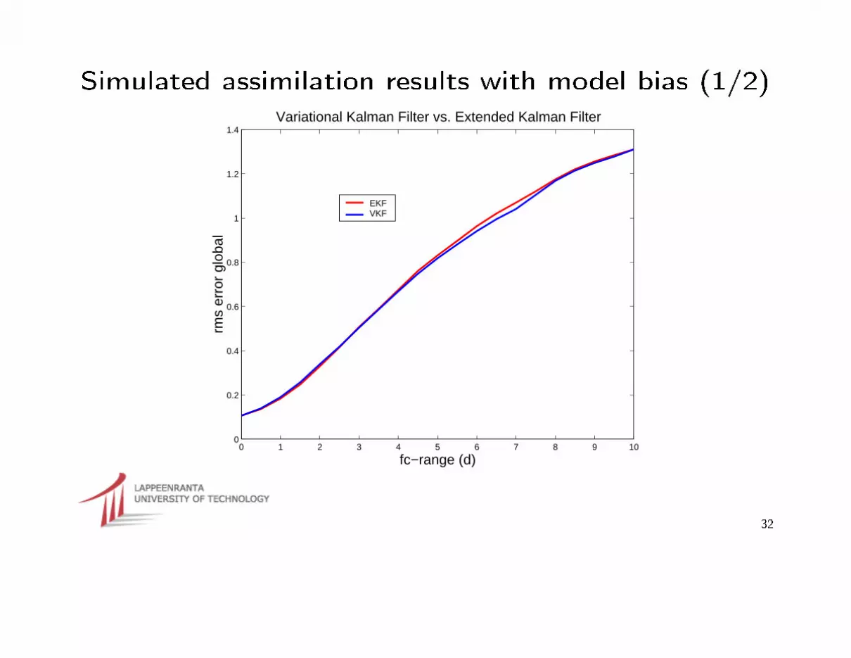
Simulated assimilation results with model bias (1/2)

0 1 2 3 4 5 6 7 8 9 100

0.2

0.4

0.6

0.8

1

1.2

1.4Variational Kalman Filter vs. Extended Kalman Filter

fc−range (d)

rms

erro

r gl

obal

EKFVKF

32

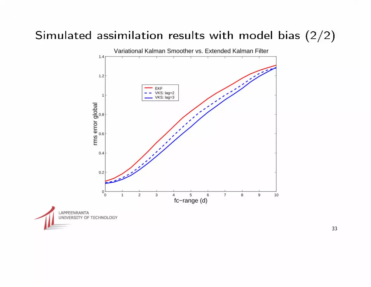
Simulated assimilation results with model bias (2/2)

0 1 2 3 4 5 6 7 8 9 100

0.2

0.4

0.6

0.8

1

1.2

1.4Variational Kalman Smoother vs. Extended Kalman Filter

fc−range (d)

rms

erro

r gl

obal

EKF VKS: lag=2VKS: lag=3

33

Conclusions

⇒ The Variational Kalman Filter (VKF) method is as good a data assimilationmethod as EKF in the Lorenz'95 benchmark

⇒ It is robust against model error⇒ It outperforms EKF, both in accuracy and in computational complexity, in

retrospective analysis⇒ It has a serial complexity comparable to that of 4D-Var⇒ It has a parallel complexity comparable to that of three subsequent model

runs with a parallelized model plus a sequence of local 4D-Var steps, and hasthe potential to outperform even the standard 4D-Var in wall-clock time on alarge parallel supercomputer

⇒ In principle, linear speedup with such a parallel complexity looks attainable oncurrent parallel supercomputers.

34

VARIATIONAL KALMAN FILTERING ON PARALLEL COMPUTERS

Documents