Valuing Employee Stock Option (ESO) With Sequential ... Employee Stock Option (ESO) With Sequential Execution Using Lattice Method Erwinna Chendra1,2, Dai Tian-Shyr3, Kuntjoro A. Sidarto4

Valuing Employee Stock Option (ESO) With Sequential Execution

Using Lattice Method

Erwinna Chendra1,2

, Dai Tian-Shyr3, Kuntjoro A. Sidarto

4

1,4

Industrial and Financial Mathematics Group, Institute of Technology Bandung, Indonesia

[email protected], [email protected]

2Department of Mathematics, Parahyangan Catholic University, Indonesia

[email protected]

3Institute of Finance, National Chiao Tung University, Taiwan

[email protected]

Abstract

Employee Stock Options (ESOs) are frequently used by a company to encourage its employees

without the burdens of immediate cash payout. How to evaluate ESOs accurately from

employees’ point of view is critical for designing effective salary systems. Empirical studies

suggest that ESOs are sequentially exercised in parts by employees. Our paper analyzes this

sequential execution phenomenon by considering the impacts of employee’s income tax and

share dilution due to exercises of ESOs. Specifically, we develop a novel forest model that

analyzes an employee’s execution strategy to maximize the present value of the lump sum of his

future disposable incomes, which is defined as his salary plus ESOs payoff minus the

progressive income tax. The forest is composed of several lattices and each lattice simulates one

possible dilution scenario. Each node of the lattice contains a table for analyzing the optimal

exercising strategy at that node. The transition among the nodes in the forest models the

sequential executions of an employee and the corresponding dilutions. Numerical experiments

are given to analyze and to verify the robustness of the lattice.

1. Introduction

Employee stock option (ESO) is a call option on the issuer’s stock granted by an issuing

company to its employees. Employees can exercise ESOs in part and may lose their unexercised

options once they resign. Thus ESOs are useful and popular financial instruments for a firm to

retain key employees and motivate them to improve the company’s performance. Unlike usual

options that can be traded by typical institutional or individual investors, employees cannot sell

or transfer their ESOs to other investors. To maintain employees’ long-term incentives, an ESO

usually has a long maturity ranged from 5 to 15 years. It is not exercisable during the first few

years of the option’s life (called the vesting period). In case an employee leaves the company

during the vesting period, then his ESOs is forfeited (i.e. ESOs become worthless). Otherwise,

the holder can repeatedly exercise his ESOs in part to optimize his/her benefits. Analyzing the

benefits for granting an employee ESOs is critical for designing effective salary systems.

In 2004, the revised Statement of Financial Accounting Standards No. 123 requests issuers to

estimate and recognize ESO’s value by adjusted option-pricing models, like the Black-Scholes-

Merton formula or the binomial lattice method, unless the market values of similar instruments

are available (FASB, 2004). Many researchers argue that using adjusted Black-Scholes model

will overprice ESOs. Hemmer et al. (1994) provide evidence that simply substituting the

expected exercise time horizon for the time to maturity of ESO in the Black-Scholes model tend

to significantly overvalue the ESOs. To address this problem, they first estimate the Greek letter

“Theta”— the sensitivity of a European-style ESO’s price to the change of the time to maturity.

The fair ESO value is then estimated as the value of an otherwise identical European-style ESO

matured at the end of the vesting period plus the product of negative Theta and the expected time

horizon minus the length of vesting period. Carpenter et al. (2010) conduct a comprehensive

study of the optimal exercise policy of a risk-averse executive and its implications for firm cost.

They compare the true option cost and their model’s option value with the adjusted Black-

Scholes and show that the error can be large or small, positive or negative, depending on firm

characteristics.

Recent papers analyze behaviors of exercising ESOs and hence evaluations by considering

employees’ desires to maximize their utilities, like Lambert et al (1991), Huddart (1994),

Kulatilaka and Marcus (1994), Carpenter (1998), Detemple and Sundaresan (1999), and Hall and

Murphy (2002). Lambert et al. (1991) use certainty equivalence approach and define the value of

ESO as a lump-sum payment of employee’s wealth, which is defined as ESO’s payoff plus

employee’s other wealth, such that the employee is indifferent between receiving the payoff to

exercise ESOs immediately and receiving future uncertain payoff by excising ESOs afterward,

given the structure of the rest of his wealth. These payments are based on the employee’s

expected utility. Huddart (1994) uses the von Neumann-Morgenstern utility (power utility)

function and assume that the tax deduction rate for the company is constant over time. Kulatilaka

and Marcus (1994) model explicitly accounts for an early exercise feature and treat exercise as

an all-or-nothing decision; it does not allow for partial execution. Carpenter (1998) compares a

simple extension of binomial method for the ordinary American option model, which introduces

random, exogenous exercise and forfeiture, with the utility maximizing model which also

includes the employee’s risk aversion, outside wealth and potential gain but ignores the presence

of taxes. She concludes that a simple American option pricing model can describe actual option

exercises just as well as a complex utility-based model. Detemple and Sundaresan (1999)’s

model relies on simple dynamic programming techniques and they assume that the employee

also invests into a risky portfolio. Hall and Murphy (2002) analyze ESO values and early

exercise decisions using a modified binomial approach with two major differences, i.e. based on

CAPM expected returns and compare the expected utility from exercising to the expected utility

from holding the option for another period. They also ignore taxes so the stock acquired through

exercise is sold immediately, with the cash proceeds invested at the risk-free rate. The main

disadvantage of using utility maximizing models is that risk aversion levels are unobserved so

we need to calibrate utility maximizing models to the data. Besides that, it might be hard to

determine the appropriate utility function that suits for all employees. That’s why we use the risk

neutral valuation approach rather than the utility based approach.

There are some papers that distinguish the ESO value for the employee (the subjective value)

and the cost of ESO to the company (the objective value). For example, Ingersoll (2006) uses the

constrained portfolio optimization method to solve for the optimal portfolio of the undiversified

manager and then determines the employee’s indirect utility function. The marginal utility is then

used as a subjective state price density to value ESO. He found that the objective value lies

between the subjective value and the market. However, if the objective value is larger than the

subjective value then the firm may give compensations directly instead of ESO. In this paper, we

analyze the valuation of an ESO from the employee’s perspective.

We modified the Cox, Ross, and Rubinstein (CRR) binomial method to price an ESO which is

similar to Aboody (1996), Hull and White (2004), Ammann and Seiz (2004), Bajaj et al. (2006),

and Brisley and Anderson (2007). Aboody (1996) uses modified CRR model that account for

unique characteristics of ESO, such as: employee exit rate, vesting period, and non-

transferability. He also consider about a tax deduction for the company, which is assumed to be

constant. Hull and White (2004) propose enhanced FASB 123 model with binomial method that

considers the vesting period, the possibility that employees will leave the company during the

life of the option, and the sale restriction. They model the early exercise behavior by assuming

that exercise takes place whenever the stock price reaches a constant multiple of the strike price

and the option has vested. Ammann and Seiz (2004) propose enhanced American model with

binomial method. This model is similar to the American model adjusted for the exit rate and the

vesting period and explicitly incorporates the employee’s early exercise policy which is assumed

that exercise take place whenever there is a positive intrinsic value and the adjusted exercise

value is larger than the holding value. The adjustment factor in the exercise value (i.e. the

adjusted strike price) is used only to determine the exercise policy, not to calculate the payoff of

the ESO. However, empirical studies find that employees require the stock price to be at

relatively high to induce voluntary exercise, yet later they will exercise at relatively low stock

price near the time to maturity. Regarding to that, Brisley and Anderson (2007) propose 𝜇-model

which assumes that employees exercise voluntary if the moneyness of the option reaches a fixed

proportion, 𝜇, of its remaining Black-Scholes value. Bajaj et al. (2006) develop an ESO

valuation model that incorporates the various unobservable factors (such as the ESO’s in-the-

moneyness, the grant’s remaining contractual life, employees’ historical exercise, the stock’s

volatility, blackout periods, and employees’ ages and lengths of service) that could influence an

employee’s early exercise decision at each lattice node, through an estimated early exercise

probability. This probability of early exercise of a vested and exercisable option at a particular

node on the lattice is expressed as a two-dimensional matrix, i.e., as a function of the ESO’s

remaining vested life and its in-the-moneyness at that particular node. Cvitanic et al. (2008)

introduce an ESO model that captures the early exercise feature and derive an analytic formula

for the ESO’s price. All of these papers set the exercise policy exogenously, assuming a single

stock price boundary, to model the early exercise feature.

Many previous empirical studies, such as Hemmer et. al. (1994), Aboody (1996), and Huddart

and Lang (1996), emphasize that employees would prefer to distribute the execution of their

ESOs over multiple dates, which is called sequential execution phenomenon, rather than execute

all of their options at a single date. In other words, employee executions are spread over the life

of the ESOs. This paper provides a model which is consistent with this empirical evidence. ESO

as part of employee compensation packages will affect the amount of tax to be paid by the

employee. Depending upon the tax treatment of stock options granted to employees, they can be

classified as either qualified/incentive stock options (ISO) or non-qualified stock options

(NQSO). Exercising ISO pays capital gain tax which is usually lower than the income tax paid

by exercising NQSO. Companies typically prefer to grant NQSO because they can deduct the

cost incurred for NQSO as an operating expense sooner. We only focus on non-qualified stock

options (NQSO). Huddart and Lang (1996) analyze the employee exercise behavior, that it is

strongly associated with stock price movements, the-market-to-strike ratio, the remaining option

life, the vesting period, and so on. Although they did not do the analysis for personal tax rate,

they also admit that it may affect exercise behavior as well. The first contribution of this paper is

to analyze sequential execution phenomenon by considering the impacts of employee’s income

tax. The progressive income tax mechanism is widely used in many countries so exercising too

many ESOs would significantly increase the tax burden under this mechanism. On the other

hand, postponing executions of ESOs would result in loss of time value. The optimized ESO

execution strategy can be quantitatively analyzed as the one to maximize the present value of the

lump sum of his future disposable incomes, which is defined as his salary plus ESOs payoff

minus the income tax, using lattice method. Each node of the lattice contains a table for

analyzing the optimal exercising strategy at that node.

This sequential execution model is similar to performance based ESO that was awarded to

Merrill Lynch’s CEO, Mr John A Thain in late 2007 (see Bernard and Boyle (2011)). Mr Thain

was granted 1,800,000 ESOs that come in three tranches: 600,000 ESOs that vest and become

exercisable after two years, 600,000 ESOs that vest and become exercisable if the average of

Merrill’s stock price is above some price (the first target price), and 600,000 ESOs that vest and

become exercisable if the average of Merrill’s stock price is above the second target price. This

is also partial execution model for ESO with different strike price and Bernard and Boyle (2009)

use Monte Carlo method to price it.

The other papers that consider about sequential execution are Jain and Subramanian (2004),

Rogers and Scheinkman (2007), Grasselli and Henderson (2009), and Leung and Sircar (2009).

Jain and Subramanian (2004) propose a multi period binomial model to value ESO assuming that

the employee has preferences over distributions of intertemporal cash flows from option exercise

(allowing for the possibility that the employee strategically exercises her options over time rather

than at a single date). The employee’s intertemporal preferences are described by the

monotonically increasing, concave, utility function. Rogers and Scheinkman (2007) consider

ESO as an American-style call option with the sale restriction and assume that the employee can

exercise parts of the option at any time and deposit the proceeds from the exercise in a risk-free

account. They develop a second-order non-linear PDE with suitable boundary conditions and

solve it numerically. Grasselli and Henderson (2009) show that risk aversion and incomplete

market causes the employee to exercise ESO in a small number of large blocks and the exercise

policy depend on the current stock price, current wealth, the number of ESO remaining, and the

ESO’s time-to-maturity. Leung and Sircar (2009) use a chain of nonlinear free-boundary

problems of reaction-diffusion type that accounts for risk aversion, vesting, job termination risk,

and multiple exercises to valuate ESO.

It is undeniable that the “fair value of ESO” is recognized as an expense in the company income

statement. As an expense, ESO would reduce reported earnings per share (EPS) and possibly

undermines share prices because exercising ESO leads to issuance of new shares. Those newly

issued shares increase the number of outstanding shares. These lead to the economic dilution of

ESO. This dilution effect raises “double accounting” issue. Some experts also argue that ESO is

more like contingent liability than equity transactions (see Balsam (1994), Kirschenheiter et al.

(2004), AAA-FASC (2004), Ohlson and Penman (2007), and Landsman et al. (2006)). Their

argument is that equity-settled ESO is economically equivalent to cash-settled ESO, so they

should be accounted for in the same manner. Cash-settled ESO is recognized as liability because

it is an obligation to transfer cash or other assets. Kirschenheiter et al. (2004) also mention that if

ESO is recognized as liability then there is no need to calculate diluted EPS, hence there is no

“double accounting” problem. In this paper, we will show that we do not fully agree with this

“double accounting” opinion. We will also consider about dilution effect from exercising ESO.

That is the second contribution of this paper. We develop a novel forest model, that is composed

of several lattices and each lattice simulates one possible dilution scenario. The transition among

the nodes in the forest models the sequential executions of an employee and the corresponding

dilutions. This model is similar to the model for evaluating corporate bonds with complex debt

structure (see Liu et al. (2016)).

The remaining paper is organized as follows. The sequential execution phenomena for ESOs can

be modeled by maximizing a holder’s benefit prescribed by the present value of disposable

incomes under the impacts of progressive tax mechanism in Section 2. Exercising ESOs would

dilute existing equity and change the issuer’s capital structure. These changes can be modeled by

taking advantages of the forest structure in Section 3. Section 4 examines the robustness of our

numerical method and analyzes the properties of ESOs. Section 5 concludes the paper and

discusses possible future extensions.

2. Preliminaries

Like other exchange-traded stock options, an ESO holder can also exercise the option to

purchase the underlying stock with the strike price 𝐾 prior to the maturity date. Usually, the

strike price is the prevailing price of the underlying stock (i.e. the initial stock price) at the time

of issue. For convenience, an ESO is assumed to be issued at time 0 and mature at time 𝑇. The

longer the maturity date, the ESO holder has a greater opportunity to exercise it. Most ESO

contracts do not allow holders to immediately exercise ESOs until the end of the so-called,

vesting period. If ESO holders leave their jobs during the vesting period then they lose their

unvested ESO. In addition, ESO holders may be forced to exercise their unexercised but vested

ESOs upon leaving the company. To consider these phenomena, much ESO evaluation

literatures (e.g. Ammann and Seiz (2004), Brisley and Anderson.(2008), Cvitanic et. al. (2008),

Hull and White. (2004), Ingersoll (2006), and Leung and Sircar.(2009)) model the employee

turnover rate as constants or by Poisson processes. This paper focuses on developing a novel

lattice, the state transition lattice, to model how ESO holders optimize their disposable incomes

under progressive income tax systems. Both vesting periods and turnover rates can be easily

inserted into our lattice without difficulty and will only be briefly explained later for simplicity.

The underlying stock price at time 𝑡, 𝑆𝑡, is assumed to follows the lognormal diffusion process

described as follows:

𝑆𝑡+𝑑𝑡 = 𝑆𝑡 ∙ 𝑒[(𝑟−𝑜.5𝜎2)𝑑𝑡+𝜎𝑑𝑊𝑡] , (1)

where 𝑊𝑡 is the standard Wiener process, r is a riskless interest rate, and 𝜎 is the volatility of the

stock price. This paper models the stock price process with the CRR binomial lattice method (see

Cox et al. (1979)) as illustrated in Figure 1. It equally divides the lifespan of ESOs into n discrete

time steps1 and the length of a time step ∆𝑡 =

𝑇

𝑛. The stock price and the index of each node

(illustrated by a rectangle for the root node or an upper right triangle for others) are listed at the

top of the node. The node index (𝑖, 𝑗) denotes as the j-th node (calculated from the bottom) at

time step i (or at time 𝑖∆𝑡). The initial stock price at the root node (0,0) is denoted by 𝑆0. It can

either go up to 𝑆0𝑢 with probability 𝑝 =𝑒𝑟∆𝑡−𝑑

𝑢−𝑑 or go down to 𝑆0𝑑 with probability 1 − 𝑝, where

𝑢 = 𝑒𝜎√∆𝑡 and 𝑑 =1

𝑢. Similarly, each stock price can either move up or down at subsequent time

steps; therefore, the stock price at node (𝑖, 𝑗) 𝑆𝑖,𝑗, is 𝑆0𝑢𝑗𝑑𝑖−𝑗. Note that the price process

modeled by the CRR binomial lattice converges to the lognormal stock price process in equation

(1) as the number of time steps 𝑛 of the lattice increases.

3. Sequential Execution Model for ESOs

To analyze the sequential execution behaviors of ESO holders, we introduce a novel numerical

model, a state transition lattice that models how different ESOs execution strategies change the

issuer’s capital structure, dilute the value existing shares, and hence influence the benefits of

ESO holders as illustrated in Figure 1.

Figure 1 A Two-Time-Step State Transition Lattice

1 𝑛 = 2 in Figure 1.

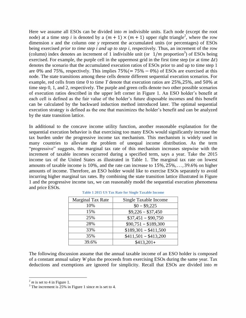
Here we assume all ESOs can be divided into m indivisible units. Each node (except the root

node) at a time step i is denoted by a (𝑚 + 1) × (𝑚 + 1) upper right triangle2, where the row

dimension x and the column one y represent the accumulated units (or percentages) of ESOs

being exercised prior to time step i and up to step i, respectively. Thus, an increment of the row

(column) index denotes an increment of 1 indivisible unit (or 1/𝑚 proportion3) of ESOs being

exercised. For example, the purple cell in the uppermost grid in the first time step (or at time ∆𝑡)

denotes the scenario that the accumulated execution ratios of ESOs prior to and up to time step 1

are 0% and 75%, respectively. This implies 75%(= 75% − 0%) of ESOs are exercised at this

node. The state transitions among these cells denote different sequential execution scenarios. For

example, red cells from time 0 to time T denote that execution ratios are 25%,25%, and 50% at

time step 0, 1, and 2, respectively. The purple and green cells denote two other possible scenarios

of execution ratios described in the upper left corner in Figure 1. An ESO holder’s benefit at

each cell is defined as the fair value of the holder’s future disposable incomes and this benefit

can be calculated by the backward induction method introduced later. The optimal sequential

execution strategy is defined as the one that maximizes the holder’s benefit and can be analyzed

by the state transition lattice.

In additional to the concave income utility function, another reasonable explanation for the

sequential execution behavior is that exercising too many ESOs would significantly increase the

tax burden under the progressive income tax mechanism. This mechanism is widely used in

many countries to alleviate the problem of unequal income distribution. As the term

“progressive” suggests, the marginal tax rate of this mechanism increases stepwise with the

increment of taxable incomes occurred during a specified term, says a year. Take the 2015

income tax of the United States as illustrated in Table 1. The marginal tax rate on lowest

amounts of taxable income is 10%, and the rate can increase to 15%, 25%, . . . , 39.6% on higher

amounts of income. Therefore, an ESO holder would like to exercise ESOs separately to avoid

incurring higher marginal tax rates. By combining the state transition lattice illustrated in Figure

1 and the progressive income tax, we can reasonably model the sequential execution phenomena

and price ESOs. Table 1 2015 US Tax Rate for Single Taxable Income

Marginal Tax Rate Single Taxable Income

10% $0 − $9,225

15% $9,226 − $37,450

25% $37,451 − $90,750

28% $90,751 − $189,300

33% $189,301 − $411,500

35% $411,501 − $413,200

39.6% $413,201+

The following discussion assume that the annual taxable income of an ESO holder is composed

of a constant annual salary W plus the proceeds from exercising ESOs during the same year. Tax

deductions and exemptions are ignored for simplicity. Recall that ESOs are divided into m

2 m is set to 4 in Figure 1.

3 The increment is 25% in Figure 1 since m is set to 4.

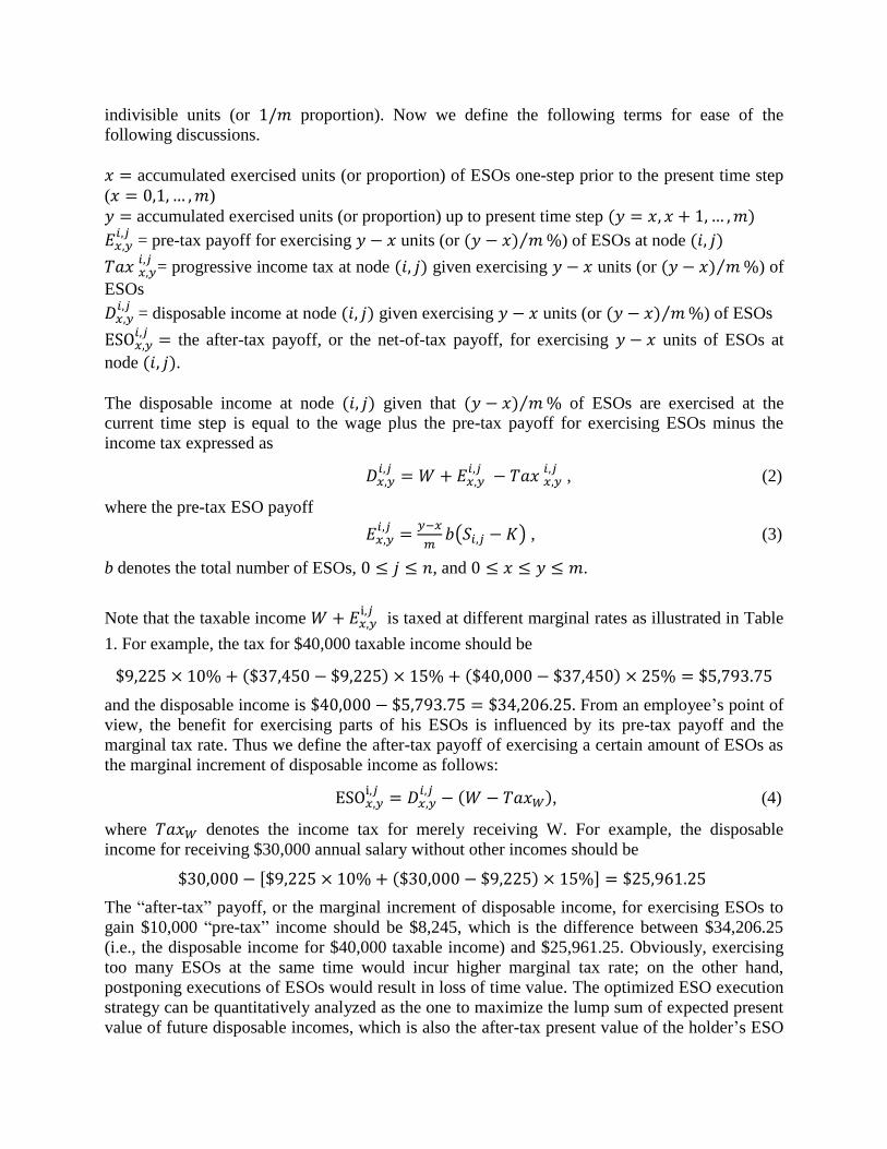
indivisible units (or 1/𝑚 proportion). Now we define the following terms for ease of the

following discussions.

𝑥 = accumulated exercised units (or proportion) of ESOs one-step prior to the present time step

(𝑥 = 0,1, … , 𝑚)

𝑦 = accumulated exercised units (or proportion) up to present time step (𝑦 = 𝑥, 𝑥 + 1, … , 𝑚)

𝐸𝑥,𝑦𝑖,𝑗

= pre-tax payoff for exercising 𝑦 − 𝑥 units (or (𝑦 − 𝑥) 𝑚⁄ %) of ESOs at node (𝑖, 𝑗)

𝑇𝑎𝑥 𝑥,𝑦𝑖,𝑗

= progressive income tax at node (𝑖, 𝑗) given exercising 𝑦 − 𝑥 units (or (𝑦 − 𝑥) 𝑚⁄ %) of

ESOs

𝐷𝑥,𝑦𝑖,𝑗

= disposable income at node (𝑖, 𝑗) given exercising 𝑦 − 𝑥 units (or (𝑦 − 𝑥) 𝑚⁄ %) of ESOs

ESO𝑥,𝑦𝑖,𝑗

= the after-tax payoff, or the net-of-tax payoff, for exercising 𝑦 − 𝑥 units of ESOs at

node (𝑖, 𝑗).

The disposable income at node (𝑖, 𝑗) given that (𝑦 − 𝑥) 𝑚⁄ % of ESOs are exercised at the

current time step is equal to the wage plus the pre-tax payoff for exercising ESOs minus the

income tax expressed as

𝐷𝑥,𝑦𝑖,𝑗

= 𝑊 + 𝐸𝑥,𝑦𝑖,𝑗

− 𝑇𝑎𝑥 𝑥,𝑦𝑖,𝑗

, (2)

where the pre-tax ESO payoff

𝐸𝑥,𝑦𝑖,𝑗

=𝑦−𝑥

𝑚𝑏(𝑆𝑖,𝑗 − 𝐾) , (3)

b denotes the total number of ESOs, 0 ≤ 𝑗 ≤ 𝑛, and 0 ≤ 𝑥 ≤ 𝑦 ≤ 𝑚.

Note that the taxable income 𝑊 + 𝐸𝑥,𝑦i,𝑗

is taxed at different marginal rates as illustrated in Table

1. For example, the tax for $40,000 taxable income should be

$9,225 × 10% + ($37,450 − $9,225) × 15% + ($40,000 − $37,450) × 25% = $5,793.75

and the disposable income is $40,000 − $5,793.75 = $34,206.25. From an employee’s point of

view, the benefit for exercising parts of his ESOs is influenced by its pre-tax payoff and the

marginal tax rate. Thus we define the after-tax payoff of exercising a certain amount of ESOs as

the marginal increment of disposable income as follows:

ESO𝑥,𝑦i,𝑗

= 𝐷𝑥,𝑦𝑖,𝑗

− (𝑊 − 𝑇𝑎𝑥𝑊), (4)

where 𝑇𝑎𝑥𝑊 denotes the income tax for merely receiving W. For example, the disposable

income for receiving $30,000 annual salary without other incomes should be

$30,000 − [$9,225 × 10% + ($30,000 − $9,225) × 15%] = $25,961.25

The “after-tax” payoff, or the marginal increment of disposable income, for exercising ESOs to

gain $10,000 “pre-tax” income should be $8,245, which is the difference between $34,206.25

(i.e., the disposable income for $40,000 taxable income) and $25,961.25. Obviously, exercising

too many ESOs at the same time would incur higher marginal tax rate; on the other hand,

postponing executions of ESOs would result in loss of time value. The optimized ESO execution

strategy can be quantitatively analyzed as the one to maximize the lump sum of expected present

value of future disposable incomes, which is also the after-tax present value of the holder’s ESO

and future salaries evaluated under the risk-neutral valuation method. The value of ESOs can be

evaluated as the lump sum expected present values of their after-tax payoffs implied by the

aforementioned optimal execution strategy.

The optimal execution strategy and hence the value of ESOs for an arbitrary node (𝑖, 𝑗) in the

state transition lattice can be determined backwardly from the last time step n to time step 0 by

applying the following recursive formulas. Let 𝑀𝐷𝑥𝑖,𝑗

denote the maximum present value of

disposable incomes received from time step i to maturity given that 𝑥 𝑚⁄ % of ESOs are already

exercised prior to time step 𝑖. At the maturity (i.e. 𝑖 = 𝑛), an ESO holder will choose an optimal

accumulated execution ratio 𝑦′ that maximize 𝑀𝐷𝑥𝑛,𝑗

as follows

𝑀𝐷𝑥𝑛,𝑗

= 𝐷𝑥,𝑦′𝑛,𝑗

= max𝑥≤𝑦≤𝑚

[𝐷𝑥,𝑦𝑛,𝑗

] = max𝑥≤𝑦≤𝑚

[(𝑊 + 𝐸𝑥,𝑦𝑛,𝑗

) − 𝑇𝑎𝑥𝑥,𝑦𝑛,𝑗

]. (5)

The after-tax value for ESO at node (𝑛, 𝑗) implied by the optimal strategy 𝑦′ is

VESO𝑥𝑛,𝑗

= ESO𝑥,𝑦′n,𝑗

= 𝐷𝑥,𝑦′𝑛,𝑗

− (𝑊 − 𝑇𝑎𝑥𝑊). (6)

For a lattice node prior to maturity, its optimal execution strategy and corresponding values of

ESOs and disposable incomes can be calculated by the backward induction procedure. Note that

an ESO holder would pick his optimal exercise amount 𝑦 − 𝑥 at node (𝑖, 𝑗) to maximize the

present value of disposable incomes received from time step 𝑖 to maturity described as follows

𝑀𝐷𝑥𝑖,𝑗

= max𝑥≤𝑦≤𝑚[𝐷𝑥,𝑦𝑖,𝑗

+ EP𝑉𝑦𝑖,𝑗

], (7)

where EP𝑉𝑦𝑖,𝑗

denotes the present value at node (𝑖, 𝑗) of future disposable incomes received from

time step 𝑖 + 1 to ESO’s maturity given that the accumulated execution ratio is (𝑦/𝑚)%. Based

on the outgoing binomial structure of the CRR lattice illustrated in Figure 1, EP𝑉𝑦𝑖,𝑗

can be

evaluated by the backward induction procedure described as follows

EP𝑉𝑦𝑖,𝑗

= 𝑒−𝑟∆𝑡[𝑝 ∙ 𝑀𝐷𝑦𝑖+1,𝑗+1

+ (1 − 𝑝) ∙ 𝑀𝐷𝑦𝑖+1,𝑗

]. (8)

Let the optimal accumulated execution ratio that maximize the right hand side of Eq. (7) be 𝑦′. The after-tax ESO value under the optimal exercise strategy can be evaluated as

VESO𝑥𝑖,𝑗

= ESO𝑥,𝑦′𝑖,𝑗

+ 𝑒−𝑟∆𝑡[𝑝 ∙ VESO𝑦′𝑖+1,𝑗+1

+ (1 − 𝑝) ∙ VESO𝑦′𝑖+1,𝑗

]. (9)

By repeatedly applying Equations (7), (8), and (9) alternatively from time step 𝑛 − 1 back to

time step 0, we can obtain the optimal execution strategy, the corresponding payoff for

exercising ESOs, and the disposable income at each node. The fair value of ESO evaluated by

the state transition lattice is the after-tax ESO value at the root node; that is, VESO00,0

.

The above model can be extended to deal with the vesting period and the turnover rate. Note that

a holder cannot exercise his/her ESOs during the vesting period and complex backward

induction for determining optimal sequential execution is not required. Take the vesting period

that ends at time step 1 in Figure 2 for example. An ESO holder cannot exercise any ESOs at

time step 0 and only one state is required at the root node. The dimension of previous

accumulated execution ratio of ESOs for the nodes in time step 1 is not required since no ESOs

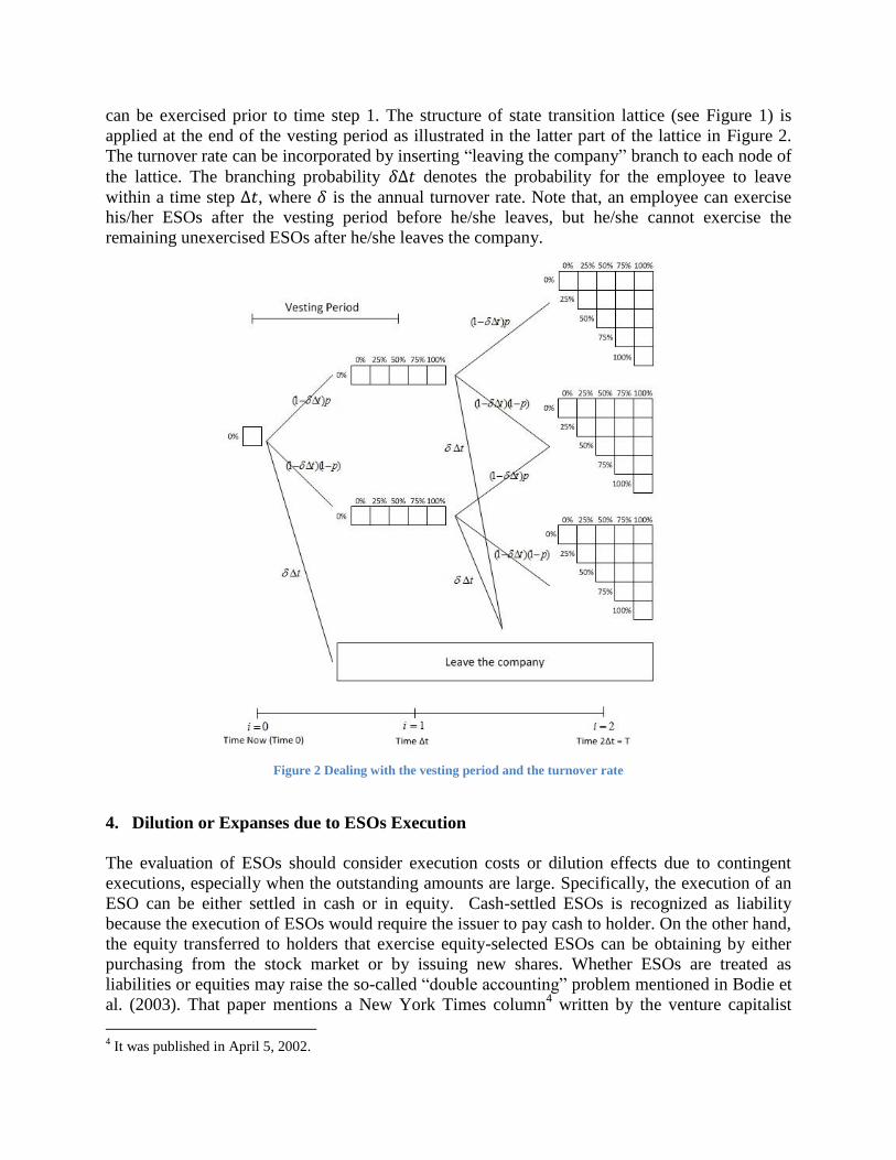
can be exercised prior to time step 1. The structure of state transition lattice (see Figure 1) is

applied at the end of the vesting period as illustrated in the latter part of the lattice in Figure 2.

The turnover rate can be incorporated by inserting “leaving the company” branch to each node of

the lattice. The branching probability 𝛿Δ𝑡 denotes the probability for the employee to leave

within a time step Δ𝑡, where 𝛿 is the annual turnover rate. Note that, an employee can exercise

his/her ESOs after the vesting period before he/she leaves, but he/she cannot exercise the

remaining unexercised ESOs after he/she leaves the company.

Figure 2 Dealing with the vesting period and the turnover rate

4. Dilution or Expanses due to ESOs Execution

The evaluation of ESOs should consider execution costs or dilution effects due to contingent

executions, especially when the outstanding amounts are large. Specifically, the execution of an

ESO can be either settled in cash or in equity. Cash-settled ESOs is recognized as liability

because the execution of ESOs would require the issuer to pay cash to holder. On the other hand,

the equity transferred to holders that exercise equity-selected ESOs can be obtaining by either

purchasing from the stock market or by issuing new shares. Whether ESOs are treated as

liabilities or equities may raise the so-called “double accounting” problem mentioned in Bodie et

al. (2003). That paper mentions a New York Times column4 written by the venture capitalist

4 It was published in April 5, 2002.

John Doerr and FedEx CEO Frederick Smith that reads “the impact of options would be counted

twice in the earnings per share: first as a potential dilution of the earnings, by increasing the

shares outstanding, and second as a charge against reported earnings. The result would be

inaccurate and misleading earnings per share”. To fairly evaluate the impacts of ESOs executions

on the prevailing stock price and hence the payoffs of executions without causing the

aforementioned double accounting problem, two evaluation methods that consider solely

execution expenses and dilution effects are discussed as follows. Let us consider a simple case

that the firm grants 𝛽 shares to ESOs holder at maturity due to executions. If these shares are

purchased from the market, the after-settlement stock price 𝑆′ should be

𝑆′ =𝑉−𝐷−𝛽𝑆+𝛽𝐾

𝛼 , (10)

where 𝑉 is the firm value, 𝐷 is the amount of due debt, 𝑆 denotes the price for the firm to

purchase the stocks, 𝐾 is the ESO strike price, and 𝛼 is the number of outstanding shares. To

solve Equation (10) with two unknowns 𝑆 and 𝑆′, we add one more constraint 𝑆 = 𝑆′ due to the

arbitrage-free argument described as follows. Assume that 𝑆′ > 𝑆 then someone can borrow 𝛽𝑆

dollars to buy stock and at ESO maturity he gets 𝛽(𝑆′ − 𝑆) dollars. If 𝑆′ < 𝑆 then he can sell 𝛽

shares to get 𝛽𝑆 dollars and at ESO maturity he gets 𝛽(𝑆 − 𝑆′) dollars. So 𝑆′ should be equal to

𝑆 because if they are not equal then there is an arbitrage opportunity. If the company issues new

shares, then at debt and ESO maturity, the stock price becomes

𝑆′ =𝑉−𝐷+𝛽𝐾

𝛼+𝛽 (11)

For cash-settled ESO, at debt and ESO maturity we have new equity value as

𝑉 − 𝐷 − 𝛽(𝑆 − 𝐾)

and if we divide it by the number of outstanding shares, we also have equation (10). So we can

say that equity-settled ESO by purchasing old shares is economically equivalent to cash-settled

ESO. But this is not true if the company issues new shares. From equation (10), we can see that

𝛽(𝑆 − 𝐾) is the cost and there is no dilution in the denominator of equation (10). As well as the

equation (11), there is no cost in the numerator and the dilution effect occurs from the

denominator of equation (11). So we can argue there is not “double accounting” problem with

equity-settled ESO or cash-settled ESO from model point of view.

Next, we consider dilution effect of ESO in our sequential execution model. We will use the

forest model to price ESO with sequential execution and dilution effect. The forest model is

composed of several lattices and each lattice simulates one possible dilution scenario. The

transition among the nodes in the forest models the sequential executions of an employee and the

corresponding dilutions. We modify the bino-trinomial (BTT) method by Dai and Lyuu (2010)

that uses trinomial structure to connect the diluted stock price to others CRR binomial lattices

that represent possible capital structures.

The following discussions only focus on equity-settled ESO by issuance new shares. Again we

assume that all ESOs can be divided into 4 indivisible units (𝑚 = 4). Then we have 5(= 𝑚 + 1)

layers of CRR binomial lattice, which each lattice represents one possible capital structure.

Assume the initial stock price for the 1st CRR lattice (when 0% of ESO being executed) is 𝑆0

1,

then we can build the x-th (𝑥 = 2, … , 𝑚 + 1) CRR lattice with

𝑆0𝑥 =

𝑆01𝜔+𝐾

𝑥−1

𝑚𝑏

𝜔+𝑥−1

𝑚𝑏

(12)

as the initial stock price, where K is strike price, 𝜔 is the number of outstanding shares before the

exercise of ESO and 𝑏 is the total number of ESO. Then the stock price at node (𝑖, 𝑗) in the x-th

layer CRR lattice is:

𝑆𝑖,𝑗𝑥 = 𝑆0

𝑥𝑢𝑗𝑑𝑖−𝑗 (13)

with 𝑢, 𝑑, and p as before. At the maturity date (time step n), the pre-tax for exercising 𝑦 − 𝑥

units of ESOs payoff is

𝐸𝑥,𝑦𝑛,𝑗

=𝑦−𝑥

𝑚𝑏 (

𝑆𝑛,𝑗𝑥 [𝜔+

𝑥−1

𝑚𝑏]+𝐾

𝑦−𝑥

𝑚𝑏

𝜔+𝑦−1

𝑚𝑏

− 𝐾) (14)

0 ≤ 𝑗 ≤ 𝑛, and 0 ≤ 𝑥 ≤ 𝑦 ≤ 𝑚. An ESO holder will choose an optimal execution ratio to

maximize his/her disposable income 𝐷𝑥,𝑦𝑛,𝑗

; that is, maximized disposable income 𝑀𝐷𝑥𝑛,𝑗

can be

evaluated using Eq. (5) and the after-tax ESO value under the optimal exercise strategy is given

by Eq. (6).

Define the stock price at node (𝑖, 𝑗) of the 1st CRR lattice as 𝑆𝑖,𝑗

1 . Assume if 25% of ESO is

executed then the stock price is diluted to 𝑆𝑖,𝑗∗ . Note that 𝑆𝑖,𝑗

∗ may not be in the 2nd

CRR lattice.

Thus we need to connect the node 𝑆𝑖,𝑗∗ with next period (𝑖 + 1) stock prices at the 2

nd CRR

lattice. We can use trinomial structure to connect 𝑆𝑖,𝑗∗ to a unique choice of three proper

following nodes, say nodes 𝑆𝑖+1,𝑘−12 , 𝑆𝑖+1,𝑘

2 and 𝑆𝑖+1,𝑘+12 , in the 2

nd CRR lattice as in Dai and

Lyuu (2010) (see Figure 3).

Define the mean function 𝜇 and the variance function Var as (see Dai an Lyuu (2010))

𝜇(𝑧) ≡ (𝑟 −𝜎2

2) 𝑧

Var(𝑧) ≡ 𝜎2𝑧

and the V-log-price of stock price V’ as ln(𝑉′ 𝑉⁄ ). By the lognormality of the stock price, the

mean and the variance of the 𝑆𝑖,𝑗∗ -log-price of 𝑆𝑖+1,𝑘−1

2 , 𝑆𝑖+1,𝑘2 and 𝑆𝑖+1,𝑘+1

2 equal to 𝜇(∆𝑡) and

Var(∆𝑡), respectively. Assume the 𝑆𝑖,𝑗∗ -log-price of 𝑆𝑖+1,𝑘

2 as �̂�, which is the closest one to 𝜇(∆𝑡)

among the 𝑆𝑖,𝑗∗ -log-price of all nodes at period (𝑖 + 1) of the 2

nd CRR lattice. Define also 𝛽, 𝛼,

and 𝛾 as the difference between �̂� and 𝜇(∆𝑡), �̂� + 2𝜎√∆𝑡 and 𝜇(∆𝑡), and �̂� − 2𝜎√∆𝑡 and 𝜇(∆𝑡),

respectively. Then the branching probabilities of node 𝑆𝑖,𝑗∗ (i.e. 𝑝𝑢, 𝑝𝑚, and 𝑝𝑑) can be derived by

matching the first two moments of the logarithmic stock price process and the sum of the

branching probabilities equal to one. In Appendix A of Dai and Lyuu (2010), we can see that the

above probabilities are valid probabilities.

Figure 3 Three layers of CRR capital structure

For 𝑖 = 𝑛 − 1, 𝑛 − 2, … ,0 and 𝑗 = 0,1, … , 𝑖, the pre-tax for exercising 𝑦 − 𝑥 units of ESOs

payoff is

𝐸𝑥,𝑦𝑖,𝑗

=𝑦 − 𝑥

𝑚𝑏 (

𝑆𝑖,𝑗𝑥 [𝜔 +

𝑥 − 1𝑚 𝑏] + 𝐾

𝑦 − 𝑥𝑚 𝑏

𝜔 +𝑦 − 1

𝑚𝑏

− 𝐾)

Again an ESOs holder will choose a strategy that optimizes his disposable income using Eq. (7).

Note that if 𝑥 = 𝑦, we do not need trinomial structure. But if 𝑥 ≠ 𝑦 then we need trinomial

structure to connect the diluted stock price at period 𝑖 with stock price at period 𝑖 + 1 in the x-th

layer CRR lattice. So if 𝑥 = 𝑦 then EPV𝑦𝑖,𝑗

in Eq. (7) is equal to Eq. (8), but if 𝑥 ≠ 𝑦 then

EPV𝑦𝑖,𝑗

= 𝑒−𝑟∆𝑡 [𝑝𝑢 ∙ 𝑀𝐷𝑦𝑖+1,𝑘+1 + 𝑝𝑚 ∙ 𝑀𝐷𝑦

𝑖+1,𝑘 + 𝑝𝑑 ∙ 𝑀𝐷𝑦𝑖+1,𝑘−1]

Let the optimal execution ratio that maximize 𝑀𝐷𝑥𝑖,𝑗

in Eq. (7) be 𝑦′. Then for 𝑥 = 𝑦 the after-

tax ESO value under the optimal exercise strategy can be evaluated using Eq. (9), but for 𝑥 ≠ 𝑦

the after-tax ESO value under the optimal exercise strategy is

VESO𝑥𝑖,𝑗

= ESO𝑥,𝑦′𝑖,𝑗

+ 𝑒−𝑟∆𝑡[𝑝𝑢 ∙ VESO𝑦′𝑖+1,𝑘+1 + 𝑝𝑚 ∙ VESO𝑦′

𝑖+1,𝑘 + 𝑝𝑑 ∙ VESO𝑦′𝑖+1,𝑘−1]

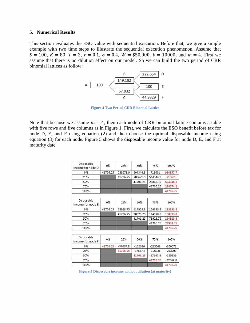
5. Numerical Results

This section evaluates the ESO value with sequential execution. Before that, we give a simple

example with two time steps to illustrate the sequential execution phenomenon. Assume that

𝑆 = 100, 𝐾 = 80, 𝑇 = 2, 𝑟 = 0.1, 𝜎 = 0.4, 𝑊 = $50,000, 𝑏 = 10000, and 𝑚 = 4. First we

assume that there is no dilution effect on our model. So we can build the two period of CRR

binomial lattices as follow:

Figure 4 Two Period CRR Binomial Lattice

Note that because we assume 𝑚 = 4, then each node of CRR binomial lattice contains a table

with five rows and five columns as in Figure 1. First, we calculate the ESO benefit before tax for

node D, E, and F using equation (2) and then choose the optimal disposable income using

equation (3) for each node. Figure 5 shows the disposable income value for node D, E, and F at

maturity date.

Figure 5 Disposable incomes without dilution (at maturity)

For node D and E, the optimal disposable income is on the fifth column, which means the

optimal strategy is executing all remaining ESOs. But for node F, the optimal strategy is not

doing execution at all. So the ESO value at these nodes is the ESO benefit corresponding to the

optimal disposable income. Then we continue backward induction to node B and C. Again, we

calculate the ESO benefit before tax and the optimal disposable income for each node using

equation (4) and equation (5), respectively. Figure 6 shows the disposable income value for node

B and C.

Figure 6 Disposable incomes without dilution (at period 1)

Again, for node C, the optimal strategy is not doing execution at all. But for node B, we can see

the sequential execution phenomenon. For example, if we have executed 25% of ESOs at the

past, then the optimal strategy is executing 25% more. But if we have executed 75% of ESO,

then the optimal strategy is not doing any execution at period 1. Similar procedure for node A

and we can get the ESO value as the ESO benefit corresponding to the optimal disposable

income. Note that there are negative disposable incomes for node F and node C in Figure 5 and

Figure 6. These because of the ESO benefit before tax at node F and C are negative. It means

that if we execute ESO at node F and C, then we will lose money, because the stock price at

these nodes is lower than the exercise price. If we get negative disposable income then the tax

will be zero.

Next, we also give a simple example to illustrate the dilution effect. We use the same data as

before and assume that the number of outstanding shares before the exercise of ESO, 𝜔, is 250.

Because we assume 𝑚 = 4, then we have five layers of CRR binomial lattices. The initial stock

prices for the 2nd

to 5th

layers can be calculated using equation (8) and others node can be

calculated using equation (8). However, extra nodes are required in low layer lattices for

trinomial lattice connection. Because they are also CRR binomial lattices, then for the l-th CRR

lattice, we can add m extra nodes above stock price 𝑆𝑖,𝑖𝑙 with 𝑆𝑖,𝑖

𝑙 𝑢2, 𝑆𝑖,𝑖𝑙 𝑢4, … , 𝑆𝑖,𝑖

𝑙 𝑢2𝑚 and m extra

nodes below stock price 𝑆𝑖,0𝑙 with 𝑆𝑖,0

𝑙 𝑑2, 𝑆𝑖,0𝑙 𝑑4, … , 𝑆𝑖,0

𝑙 𝑑2𝑚. Figure 7 shows the five layers of

CRR binomial lattices. Node X and Y are the extra nodes at period 1.

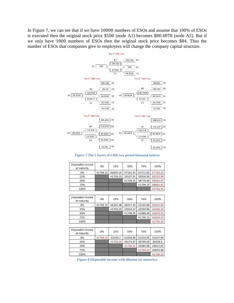
In Figure 7, we can see that if we have 10000 numbers of ESOs and assume that 100% of ESOs

is executed then the original stock price $100 (node A1) becomes $80.4878 (node A5). But if

we only have 1000 numbers of ESOs then the original stock price becomes $84. Thus the

number of ESOs that companies give to employees will change the company capital structure.

Figure 7 The 5 layers of CRR two period binomial lattices

Figure 8 Disposable income with dilution (at maturity)

At time T (period 2), we calculate the pre-tax for exercising ESOs for each node using equation

(14). Note that we use node D1 if the accumulated exercised units of ESOs one-step prior to the

present time step is 0% (𝑥 = 1), we use node D2 if the accumulated exercised units of ESOs

one-step prior to the present time step is 25% (𝑥 = 2), and so on. Then we choose the optimal

strategy that maximizes our disposable income. Figure 8 shows the disposable income value at

the maturity. We use node D1 for the first row of the top table, node D2 for the second row of

the top table, node D3 for the third row of the top table, and so on. Similarly, we use node E1 for

the first row of the middle table and node F1 for the first row of the down table, and so on.

At period 1, for example, we consider about the first row of the table (if the accumulated

exercised units of ESOs one-step prior to the present time step is 0%). Assume that the

accumulated exercised units of ESOs up to present time step is 25%, then we use trinomial

branch to connect the diluted stock price from node B1 to three unique nodes at the 2nd

CRR

lattice (node X2, D2, E2, or node D2, E2, F2). To choose the three unique nodes, first we

calculated B1-log price of all nodes and the mean-variance at period 1. Then we calculated the

“distance” between those values and the mean, and we choose the closest node as the middle

node. For that example, we get B1-log price of X2 = 0.9993, B1-log price of D2 = 0.1993, B1-

log price of E2 = -0.6007, B1-log price of F2 = -1.4007, mean = 0.02, and Var = 0.16. We can

choose node D2 as the middle node. So we connect B1 to node X2, D2, and E2 and we have

𝛽 = 0.1793, 𝛼 = 0.9793, and 𝛾 = −0.6207. The branching probabilities can be derived by

matching the first two moments of the logarithmic stock price process and the sum of the

branching probabilities equal to one. We get 𝑝𝑢 = 0.0381, 𝑝𝑚 = 0.6998, and 𝑝𝑑 = 0.2622.

Thus, at node B1, if the optimal strategy is executing 25% with past accumulation of execution is

0% (at the 1st-row and the 2

nd-column), then we calculate the pre-tax for exercising ESOs using

the trinomial structure that connect diluted stock price at node B1 with node X2, D2, and E2. In

case if the accumulated exercised units of ESOs up to present time step is 50% then we use

trinomial branch to connect the diluted stock price from node B1 to three unique nodes at the 3rd

CRR lattice (node X3, D3, and E3 or node D3, E3, and F3).

For other example, we consider about the second row of the table (the accumulated exercised

units of ESOs one-step prior to the present time step is 25%), If we assume that the accumulated

exercised units of ESOs up to present time step is also 25% then we do not need any trinomial

branch because we do not have any diluted stock price. So we just use CRR binomial

probabilities to connect the node B2 to node D2 and E2, but if the accumulated exercised units of

ESOs up to present time step is 75% then we use trinomial branch to connect the diluted stock

price from node B2 to three unique nodes at the 4th

CRR lattice (node X4, D4, E4 or node D4,

E4, and F4).

The algorithm is implemented using MATLAB on computer with processor Core™i5, RAM 4

GB, and Windows7 32-bit OS. Given the data: 𝑆 = 100, 𝐾 = 100, 𝑇 = 5, 𝑟 = 0.1, 𝜎 = 0.3,

𝑊 = $50,000, 𝑚 = 4, 𝜔 = 250, and 𝑏 = 10000. The ESO price without dilution effect is

given by Figure 9 and the ESO price with dilution effect is given by Figure 10 for different time

steps. We can see that the ESO price with dilution effect ($11.8258) is cheaper than the ESO

price without dilution effect ($46.016). If we use the same data but 𝑏 = 1000, then the ESO

price with dilution effect is $14.9944 and the ESO price without dilution effect is $46.0159. We

can see that the number of ESOs makes significant impact on the ESO price with dilution effect.

.

Figure 9 ESO Price without Dilution vs Time Step

Figure 10 ESO Price with Dilution vs Time Step

We also analyze sensitivities of ESO’s price without dilution respect to the model parameters.

Figure 11, Figure 12, Figure 13, Figure 14, and Figure 15 show how the ESO price behave as the

interest rate, the volatility, the maturity date, the amount of ESO distribution, and the total

number of ESO changes. Again, the calculations are based on the same data used by Figure 9

except for the parameter that is varied in each panel and 𝑛 = 5000.

Figure 11 ESO Price vs Interest Rate

Figure 12 ESO Price vs Volatility

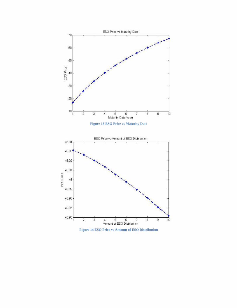
Figure 13 ESO Price vs Maturity Date

Figure 14 ESO Price vs Amount of ESO Distribution

Figure 15 ESO Price vs Total Number of ESO (with m=4)

Just as standard options, the increasing interest rate, volatility, and maturity date gives the

increasing ESO price, as shown in Figure 11, Figure 12, and Figure 13. Furthermore, the

increasing amount of ESO distribution gives the decreasing ESO price, as shown in Figure 14.

But, generally, the increasing total number of ESO also gives the increasing ESO price, see

Figure 15. There is something interesting from Figure 15, we can see that the ESO price

descends if the total number of ESO is in between 1000 to 5000. Figure 16 shows the ESO price

behaves as the total number of ESO changes between 1000 and 5000. We can see that there is a

minimum price before the ESO price increases continuously.

Figure 16 ESO Price vs Total Number of ESO with m=4 (Zoom In)

But this phenomenon does not occur if we take 𝑚 = 1 (i.e. we can only execute 0% or 100% of

ESO), the increasing total number of ESO gives the increasing ESO price continuously (see

Figure 17). We can conclude that the sequential execution will be effectively useful if the total

number of ESO is large enough.

Figure 17 ESO Price vs Total Number of ESO (with m=1)

6. Conclusion

References

[1] Aboody, D. 1996. Market valuation of employee stock options. Journal of Accounting and

Economics 22, 357-391.

[2] American Accounting Association (AAA) Financial Accounting Standards Committee

(FASC). 2004. Evaluation of the IASB's proposed accounting and disclosure requirements

for share-based payment. Accounting Horizons vol. 18 no. 1, pp. 65-76.

[3] Ammann, M. and R. Seiz. 2004. Valuing employee stock options: does the model matter?

Financial Analysts Journal, vol. 60, no. 5, pp. 21-37.

[4] Bajaj, M., S.C. Mazumdar, R. Surana, and S. Unni. 2006. A matrix-based lattice model to

value employee stock options. The Journal of Derivatives, vol. 14, no. 1, pp. 9-26.

[5] Balsam, S. 1994. Extending the method of accounting for stock appreciation rights to

employee stock options. Accounting Horizons vol. 8 no. 4 pp. 52-60.

[6] Bernard C. and P. Boyle. 2011. Monte Carlo methods for pricing discrete Parisian option.

The European Journal of Finance 17(3): 169-196.

[7] Bodie, Z., R. S. Kaplan, and R. C. Merton. 2003. For the last time: stock options are an

expense. Harvard Business Review, pp. 63-71.

[8] Brisley, N. and C.K. Anderson. 2008. Employee stock option valuation: modeling the

voluntary early exercise boundary. Financial Analysts Journal, vol. 64, no. 5, pp. 88-100.

[9] Carpenter, J. N. 1998. The exercise and valuation of executive stock options. Journal of

Financial Economics vol. 48, pp. 127-158.

[10] Carpenter, J. N., R. Stanton, and N. Wallace. 2010. Optimal exercise of executive stock

options and implications for firm cost. Journal of Financial Economics 98, 315-337.

[11] Carr, P. and V. Linetsky. 2000. The valuation of executive stock options in an intensity-

based framework. European Finance Review 4, 211-230.

[12] Cox, J., S. Ross, and M. Rubinstein. 1979. Option pricing: a simplified approach. Journal

of Financial Economics 7:229-264.

[13] Cvitanic, J., Z. Wiener, and F. Zapatero. 2008. Analytic pricing of employee stock options.

Review of Financial Studies 21, 683-724.

[14] Dai, T.S. and Lyuu Y.D. 2010. The bino-trinomial tree: a simple model for efficient and

accurate option pricing. The Journal of Derivatives, vol. 17, no. 4, pp. 7-24.

[15] Detemple, J. and S. Sundaresan. 1999. Non-traded asset valuation with portfolio

constraints: A binomial approach. Review of Financial Studies 12, 835-572.

[16] Financial Accounting Standards Board (FSAB). 2004. Statement of Financial Accounting

Standard no. 123 (revised): Share-based Payment.

[17] Grasselli, M. and V. Henderson. 2009. Risk aversion and block exercise of executive stock

options. Journal of Economic Dynamics and Control 33, 109-127.

[18] Hall, B. J. and K. J. Murphy. 2002. Stock options for undiversified executives. Journal of

Accounting and Economics 33, 3-42.

[19] Hemmer T., S. Matsunaga, and T. Shevlin. 1994. Estimating the “fair value” of employee

stock options with expected early exercise. Accounting Horizons 8, 23-42.

[20] Huddart, S. 1994. Employee stock options. Journal of Accounting and Economics 18, 207-

231.

[21] Huddart, S. and M. Lang. 1996. Employee stock option exercises: An empirical analysis.

Journal of Accounting and Economics 21, 5-43.

[22] Hull, J. and A. White. 2004. How to value employee stock options. Financial Analysts

Journal vol. 60, pp. 114-119.

[23] Ingersoll, J. E. 2006. The subjective and objective evaluation of incentive stock options.

The Journal of Business 79, 453-487.

[24] Jain, A. and A. Subramanian. 2004. The intertemporal exercise and valuation of employee

options. The Accounting Review 79, 705-743.

[25] Kirschenheiter, M., R. Mathur, and J. K. Thomas. 2004. Accounting for employee stock

options. Accounting Horizons vol. 18 no. 2 pp. 135-156.

[26] Kulatilaka N. and A. J. Marcus. 1994. Valuing employee stock options. Financial Analyst

Journal, vol. 50, no. 6, pp. 46-56.

[27] Lambert, R., D. Larcker, and R. Verrecchia. 1991. Portfolio considerations in valuing

executive compensation. Journal of Accounting Research 29, 128-149.

[28] Landsman, W. R., K. V. Peasnell, P. F. Pope, and S. Yeh. 2006. Which approach to

accounting for employee stock options best reflects market pricing? Review of Accounting

Studies 11, pp. 203-245.

[29] Leung, T. and R. Sircar. 2009. Accounting for risk aversion, vesting, job termination risk

and multiple exercises in valuation of employee stock options. Mathematical Financial 19,

99-128.

[30] Liu, L. C., T. S. Dai, and C. J. Wang. 2016. Evaluating Corporate Bonds and Analyzing

Claim Holders' Decisions with Complex Debt Structure. Journal of Banking and Finance

Forthcoming.

[31] Ohlson, J. A. and S. H. Penman. 2007. Accounting for Employee Stock Options and Other

Contingent Equity Claims: Taking a Shareholder's View. Journal of Applied Corporate

Finance 19(2): 105-110.

[32] Roger, L. C. G. and J. Scheinkman. 2007. Optimal exercise of executive stock options.

Finance and Stochastics 11, 357-372.

[33] Rubinstein, M. 1995. On the accounting valuation of employee stock options. Journal of

Derivatives, vol. 3, no. 1, pp. 8-23.

Acknowledgement

This paper is part of our research on valuing Employee Stock Options. We would like to thank

the Ministry of Research, Technology and Higher Education of the Republic of Indonesia for

financial support through 2015 PKPI Scholarship to do internship in NCTU – Taiwan.