University of St Andrews - St Andrews Research Repository

University of St Andrews

Full metadata for this thesis is available in

St Andrews Research Repository at:

http://research-repository.st-andrews.ac.uk/

This thesis is protected by original copyright

http://research-repository.st-andrews.ac.uk/

%1.1«

CONTENTS

Page

Summary 1

PART I 2

1*1) Introduction , 2

'I *2) Development of an optimal procedure 3

1 *3) Discrimination when the two populations are multivariate

normal 7

1'4) The sample discriminant function 10

1 *5) Distributions of D (x) and Dr_1(x), and misclassificationO 1

probabilities 11

1*6) The estimation of error rates 13

1*7) The analogy of discriminant analysis with regression 22

1 *8) Hypoth sis testing in discriminant analysis 26

1 *9) Size and shape factors 31

PART II 33

2*1) The population discriminant function for paired

observations, and its distribution 33

2*2) The sample discriminant function for paired -observations,

and its distribution 36

2-3) The probability of misclassification 38

2-4) The likelihood ratio criterion for the classification of

one new pair (univariate) 46

(2*5) The L.R. criterion for the classification of two new

pairs (univariate) 30

(2*6) The allocation of a single observation by the L.R.

criterion (univariate) 52

(2*7) The procedure for populations with equal means and

unequal variances

(k'8) The L.R. criterion for the classification of one new

pair (bivariate)

(2*9) The allocat ion of a single observation "by the

L.R. criterion (bivariate)

(2*10) The geometric interpretation of the discriminant

functions of (2*8) and (2'9)

(2 "11) An example of the use of DrLo

(2*12) Two algorithms for the joint classification of k

new pairs

(2*13) Conclusion

References

A

DISCRIMINANT ANALYSIS WITH RESPECT TO PAIRED OBSERVATIONS

SUMMARY

The thesis is divided into two sections. In PART I the

theory of discrim^rit analysis is presented in a standard manner.

Particular attention is paid- to those aspects of the subject which

also have relevance to-the allocation of pairs. PART II mainly concerns

the author's work on the theory of the assignment of paired observations.

It is concluded by an example which illustrates the advantages of

allocation by the discriminator developed.

c

PART I

(1*1) INTRODUCTION

In general, the problem may be stated as follows:

We are given the existence of k groups, in a population, and possess

a sample of measurements on individuals from each of the groups.

Using these measurements, we must set up a procedure whereby a new

individual can be assigned, on the basis of its own measurements,

to one of the k groups. To assess the performance of a procedure,

we usually calculate the proportion of new. individuals in each group

which we will expect to have been wrongly classified.

From an historical point of view, the first published

applications of discriminant analysis seem to have been in the papers

of Barnard (1535) and Martin (1936), both at the suggestion of R.A.Fisher.

Fisher (1936) gave another example of the methods and pointed out that

discriminant analysis was analogous to regression analysis.

P.C.Mahalanobis (1927,1930) in India and H.Retelling (193^) in-the U.S.

were concerned with similar problems. Hotelling derived the distribution. 2

of the generalised Student's ratio (T ) to test the significance of

the difference between two mean vectors. On the other hand, Mahalanobis

introduced a measure of distance between two populations (D2) as an

improvement over K.Pearson's coefficient of racial likeness, c2 (1926).Fisher (1938) showed there was a close connection between his work

3

and that'of Hotelling and Mshalanobis, while distinguishing between

the different objects for which they were developed, and derived (l9e-0)

a measure of the precision with which his discriminant function had

been calculated from the data. Until recently, the non-availability

of computers to carry out the required calculations (including the

inversion of large matrices) has deterred most people from practicing

the methods.

Discriminant Analysis should not be confused with Classification

Analysis, where we are given a sample of individuals and have to divide

them into unknown distinct groups, such that the.individuals in any

one group possess a mutual similarity.

For the remainder of the thesis we shall consider the

case of just two groups.

(1 -2) THE DEVELOPMENT OF AN OPTIMAL PROCEDURE

Let us suppose we have a large or infinite population 0,

subdivided into two populations ni and II2, and each member of II has

associated with it a p-dimensional vector of variables x. In other

words, n1 and n2 are two clusters of points in p-dimensional space,

which are separate but overlap slightly (otherwise there would be

no difficulty in distinguishing between them). A new individual has

to be assigned to I11 or n2 depending on its scores on the response

vector x.

The diagram below represents the type of situation that

arises in two dimensions. Some boundary such as A3 must be constructed,

so as to separate X's from O's in an optimal way.

/,

Three examples where Discriminant Analysis has been

successfully applied are as follows:

Variables x Populations Hi and H2

1. Anthropological measurements

on skulls

2. Sepal and Petal, length and

width

3. External symptoms in suspected

sufferers from a certain disease

Male and Female

Two species of flower e.g.

Iris Setosa and Iris Versicolor

Presence and Absence of the

disease

Now, let x have probability density function (p.d.f.)

f-f 1 (x) if x belongs to I11

hf2(x) if x belongs to II2 ,

and <£1, y>2 = 1-0i be known prior probabilities

of a member of II belonging to Hi and H2 ,respectively. It would be

desirable to split the whole p-dimensional space R into two regions

5

Ri aad Ra such that

if x falls in Ri, assign new individual to n1

cr if x falls in R2, assign new individual to n2.

By using the above procedure, we will inevitably make some wrong

decisions, and so we must choose our optimum procedure to be the

one with the smallest probability of doing so. There are two types

of error which may arise. Firstly, a new individual which is actually

from n1 may be assigned to 02 and secondly, an individual from H2 may

be classified as FIi.

Prob. (a n, individual, chosen at random, is assigned to H2)= J f1 (x)dx = di

R.2

Similarly, a2 = ff2(x)dxRi

So that, M = Prob. (a randomly chosen member of H is misallocated)= 01«1 + $2®2

= / <f>2f2(x)dx + I 01f1(x)dxRi Ra

= / 0 2 f 2 (x)dx^ + 01 - / 0ifi(x)dxRi Ri

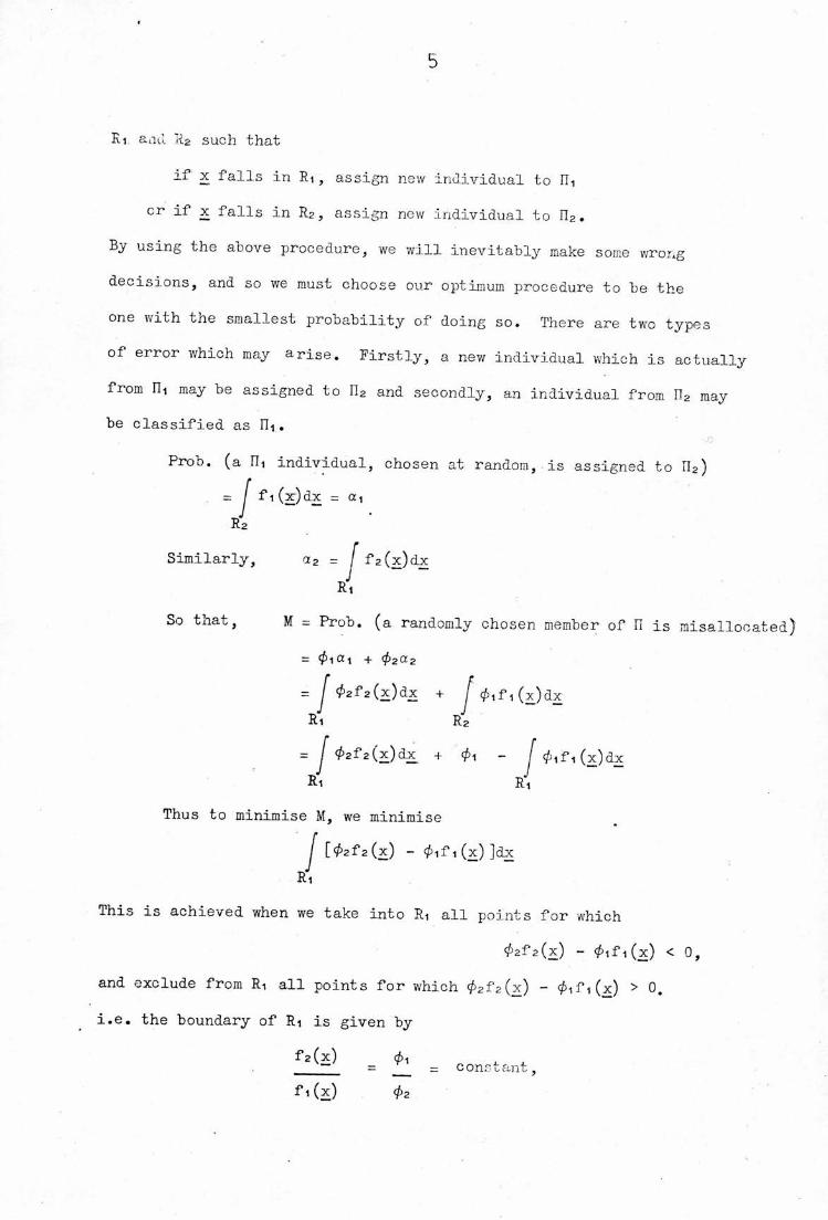
Thus to minimise M, we minimise

I [$2f2(x) - <£ifi(x)]dxRi

This is achieved when we take into Ri all points for which

</>2f2(x) - <t>ifi(x) <

and exclude from Ri all points for which 02fa(x) - 0ifi(x) > 0.

i.e. the boundary of Ri is given by

f2 (x) 01 ,—

= - constant,fi(x) 02

f 2 (x)where is the likelihood ratio for the observation x . This

f i (x)

was first proved by Welch (1939).

Looking at the problem from a more empirical angle,

we see that by a simple application of Bayes' Theorem, the conditional

probability that an observation x emanates from Hi is

01f1(g) (Anderson, 195°)f1(x) + ^2f2(x)

Now it is evident that if we assign a given observation x to that

population with the higher conditional probability, no other rule

iui smailtr misclassification probability. So if

<t> ifi(x) 4>zf 2 (x) „— > we choose II-i

0lfl(x) + 02f2(x) 0lfl(x) + 02f2(x)

If not, choose n2. Again the boundary of R1 is easily seen to reduce to

fs(x) 01

f 1 (x) 02

In the case where it is worse to misclassify members

of one population than the other, it is useful to introduce weights

ci and c 2, where

ci is the 'cost' of misclassifying an individual from nt as n2

c2 is the cost of the second type of misclsssification.

These costs may be in any units and might be introduced in circumstances

such as Example 3- , where the consequences of a wrong decision may

be drastically different viz. it is less dangerous to diagnose

presence of the disease in a healthy person, than to let the disease

go undetected in a sufferer.

We now have to minimise the expected cost 0iciai + 02C2a2

7

leading 'by similar analysis as before to the boundary of Ri being

fz(x) <£lCl

f 1 (x) ^202

We have thus the following likelihood ratio rule £, if

fi (x)> c allocate x to 311

/ f2(x)f 1 (*)

< c allocate x to n2 [1

= c allocate x to I11 with probability yf2(2£)

or to n2 with probability 1-y

When f 1 (x) an(l Pz(x) are continuous, ^ f 1 (x) -1Prob. , = c = 0, and

^ f2(x) Jthe third case does not arise. If - fi(x)

Prob. ! = c } > 0, weL f2(x) J

usually take y = -§■. In other words, if the new observation lies on

the discriminating boundary, we just spin a coin to decide which

population to assign it to.

Henceforth, we shallassume equal costs and equal prior

probabilities i.e. C1 = c2 and <£1 = $2 = so that c = 1.

(1-3) DISCRIMINATION WHEN THE TWO POPULATIONS ARE MULTIVARIATE NORMAL

We now assume Hi and PJ2 are N (Hi,£) and N (p2,S)P ~ P ~

respectively, where

£. is the vector of means in the i^*1 population (i = 1 ,2)

E is the (pxp) dispersion matrix of each population.

8

i.s. f. (x) = (2m) 12 J 2 exp -4(x ~ O x 1 (x -- £. ) (i - 1,2).L

Then log f 1 ^ 1 ,■ v ' V-1 , % 1 / - ' „-1 ,-six - £i ) (x - £1) + o(x - £2) a (x - £f2(x)

I

= [* - i(£1 + £2)] 2 (£1 - £2) = D (x)T

(by addition and subtraction of the same vector product and the property

that transpose (. $cc\ I &. r ) = (<x r )

Taking c=1 => log c =0 we see that, from [1], £ is given by

R1 is Dt(x)>0R2 is D.p(x)<0 J

[2]

and the boundary is x'2' (A£i - £2) = constant. h^(x) is usuallyknown as the Population Discriminant Function. Anderson (1958) credits

this approach to Wald(l944). Fisher(l936) arrived at the same result

by suggesting that an individual should be classified into one of the

two populations, using that linear function of its p measurements

which maximised the between group distance, relative to the within

group standard deviation. We no?/ give a matrix derivation of Fisher's

method.

Denote this linear function of x by a'x. According to

Fisher we want to maximise

la'Cifi - £2) !(a'2a)2

or equivalently, find the vector a which maximises-1

y = [a'(pi - b2)(bi - b2)'a][a'Ea]

•Cowith respectra,

= 0 => 2(£i - £2)(£i - £2) a[a'2a]-1

-a«(£1 - £2)(£i - £2) a[22a][a'2a] 2 = 0— 1 ' '

i.e. 2 (£1 - ££2) (j£i - £2) a = a'(£i - £a)(£i - £2) a

a' 2a[31

The ojily values of a that satisfy this equation are the eigenvectors-1 '

of 2 (y, - ZfsKifi ~ £2) £• The maximum of y is therefore the first

eigenvalue, with a its corresponding eigenvector.t

But Rank[ (£1 - £2) (£1 -■ £2) ] = 1-1 1

So Rank[ 2 (£1 - £e)(£i - £2) J = 1, being the product

of two matrices one of which has rank one. Therefore, there exists

only one non-zero eigenvalue.-1 1

But, sum of eigenvalues = trace (2 56 )-1 „

= ^ 2. > where 6 = £1 - £2

Substituting this value for y in [3],

ZT'S 6'a = 5'2"16 a

-1Therefore, a = mE 5 _____ [£]

6'a.where the scalar m = z—

S'2 5

As we are only attempting to separate EU and n2 (without measuring

the distance between them), m can be replaced by any ether scalar.

In other words, the coefficients of the linear discriminant function

are not unique, although their sizes are. Notice that the

values of y when a = 2 ^ (£1 - £2) is substituted reduces to1 2

(£1 - £2) 2 (£1 - £2) = D ,

2where D is Mahalanobis's Generalised Distance, i.e. the distance

2between the means on the population discriminant function is D .

Comparing [4] with D (x) , we see that Fisher's linear

discriminant function differs only by the constant

-(£1 + £2) 2" (jja ~ £2) from D (x).Thus the linear discriminant function is the best discriminator when

IIi and n2 are multivariate normal with the same dispersion matrix.

10

(1 -if) THE SAMPLE DISCRIMINANT FUNCTION"

In practice, the values of £1 ,£2 and E (the parameters

of fi and f2) are rarely known; so they are usually replaced by xi,

X2 and S, the sample means and pooled sample variance/covariance

matrix, based on samples of size m from fli and n2 from n2.

Let X1 and X2 be the (mxp) and (n2xp) matrices of sample

observations from hi and n2, respectively. Define1 1 1 «

xi = — X1 e , x2 ~ X2 eni ~ni — n2 —n2

A = Xi'(l - - E )X1 , A = X2'(I - - E )X2Ai nt m A2 r\2 riz

and S = ^"(Av + A ) whereni+n2-2v Xi X2

e (i=1 ,2) is a column vector of 1's of length n..—n. 1

x

B (i=1,2) is a (n.xn ) matrix of 1's. From now on, the 'n. 'XI. X 1 X

x

subscripts will not be included, when the dimension of the vector

or matrix of 1 's is clear.

We knew that In the multivariate normal case

x. ~ N (fi.E) independently of A^ ~ W(2,n.-1,p) (i=1,2)~~~i p in. a . 11 x

Since the samples from H-i and n2 are independent,

(m+n2-2)S ~ W(2,m+n2-2,p)

and, xi, X2 and S are unbiased estimators of £1, £2 and £. Substitution

of these estimates in D,p(x) yields the estimated likelihood ratio*

rule £ :

Dq(x) > 0 assign individual to I11If < S

D (x) < 0 assign individual to n2

where D (x) = [x - 2"(xi+£2) ] S (xi-x2) is the Sample Discriminant

Function, sometimes known as Anderson's W Statistic.

With known population parameters we argued that the

[5]

procedure was optimal since we had minimised the expected loss.

Although the above procedure [5] cannot be justified in the same

way, and will inevitably introduce further misclassification errors,

Hoel and Peterson (1049) have shown that the substitution of these

estimators produces asymptotically optimal statistics.

It is worth noting that we would have obtained D (x),O

apart from a constant term, by maximising

ja'(x, - x2)T

(a'SaY

This justifies to some extent the use of the Sample Discriminant

Function when the populations are not normal with the same covariance

matrix. Another criterion (Likelihood Ratio) is discussed, in detail,

in PART II.

(1*5) DISTRIBUTIONS OF D (x) AND D (x), AND MISCLASSIFICATION PROBABILITIESO 1

Let E_^ denote expectation with respect to f^(x) (i=1,2) .

When x belongs to IIi , D (x) is univariate normally distributed with

mean

E.tBJD! = (£1 . £o2

' -1 .2= 1 - £2) £ (Pi - £2) = 2^ , an(i variance

V£r [D^Cx)] = (£1 -£2) 2~1 ££~1(£1 -£2) = D2.p 2

Thus, if x belongs to Tin, D^,(x) ~ N(-gD _,D )2 2

Similarly, if x belongs to n2, (x) ~ N(--g-D ,D ).

The notation we adopt for misclassification probabilities

is due to Hills(1966). He defines a (0 (i=1,2) to be the probability

of misallocating a randomly chosen member of ht when C is used.

12

l h en «,(£) = Prob. ( Dt(x) < 0 I x belongs to n, )

72~ exp

1

277"

1 i^2n2 ,-^2(y-2-D ) dy

2exp --g-u du

= $(-D/2) where $ is the cumulative normal distribution

Similarly a2(0 = $(-D/2)

FIG-. 2

In FIG. 2 , ^(0 and ^(0 are represented by shaded regions cutoff at the tails of the distributions.

The unconditional distribution of D (x) is extremely

complicated, as can be observed in the works of, amongst others,

Sitgreaves(1952) and Wald(l944). Okamoto(l9^3) has worked cut an

asymptotic expansion for the distribution, up to terms of order

(Vni)2, (1/112)2, (1/n m2), 1/m (m+n2-2) , l/n2 (ni -fn2-2) , l/(m+H2-2)2.This will be considered briefly in the next chapter.

For large samples, it has been shown using limiting

13

distribution theory that, as m , 112 -* *>

xi ■* £1, "* £2 and S -» 2 , in probability.

Hence, the limiting distribution of Dq(x) is that of D (x), and forsufficiently large m , ri2 we can use the criterion as if the population

parameters were known.

However, if x belongs to n. (i=1 ,2) , D„(x) is conditionally1 O """ ""

(on xi,x2 and S) normally distributed and has mean

E.[D0(x)[xi,x2 arid S] = [p. - -1+-2] s \rxi-X2~|, and variance1

2

— ' —1 — _ —

Var[D (x)[x,,x2 and S] = [x, -x2 ] S 2S [xi-x2].

Thus_1 _ _ _ ' _i _ _

a (£*) - f ^ (i1_X2) + 1"(X1+X2)S (xi -X2)v V(xi-X2) S 'ss \xi-xz)

It is best at this stage, to make a clear distinction between*

1) a-(C ) j the conditional probability that a randomly*

chosen member of H. will be misallocated by £ ,

*

and 2) E[a (£ )] , the unconditional probability of misclassificatioA.

E denotes expectation over all possible samples of size m from ni

and n2 from n2 .

(1 *6) THE ESTIMATION OF ERROR RATES

The methods currently used to estimate the error rates

of sample discriminant functions can be divided into two categories;

in the first category, we have those assuming properties of normality

and in the second, those methods which employ sample data. The methods

dependent on normality are biased and if the degrees of freedom(n^+n -2)of the Wishart matrix S are small, may considerably underestimate the

true error rate. Their performance with non-normal distributions

is difficult to judge and, in such cases, the empirical methods of

the second category are probably more suitable. The techniques are

summarised below :

The Holdout Method (or K Method)

If the original samples X^ and are very large, wemay select a subset of observations from each, compute a discriminant

function from them and use the remainder to estimate error rates.

The number of misallocations for Hi and 02 are binomially distributed,ir- £ £

with probabilities ai(£ ) and oc2(r ). When the estimates of ai(£ )*

and a2(£ ) have been calculated, we now use the entire data set to

form the discriminant function. Since the numbers of misclassification

are binomially distributed we may also calculate confidence intervals*

/ *for a1(£ ) and a2(£ ).

The method suffers from the following disadvantages.

Firstly, large samples are not normally available in practice, for

various reasons such as cost. Secondly, the discriminant function

whose performance we have judged is not the one eventually used ;

there may be quite a difference between the two. Thirdly, different

users will obtain different estimates, since they will not select

the same subsets. Finally, we could have constructed the discriminant

function from a much smaller sample than that required for the

application of the H Method.

The Resubstitution Method (or R Method)

The method was first suggested by C.A.E.Smith (l%-7).

Quite simply, the sample used to compute the discriminant function

is reused directly, to estimate the error rates. Each observation

15

is classified, ss either I11 or H2 and we calculate nn/ni and E2/112 ,

the proportions of ITi and n2 misclassified. Again,

mi ~ Bin. (m , a<(£ )) and m2 ~ Bin. (n2 , a2(^ )).

The method has. often been found to 3îeld misleading

results - even when sample sizes are fairly large, the performance

of the discriminant function is over-optimised. Obviously, seriousJ.

bias must arise when £ is judged on the sample it was calculated

from. The advantages of the method are the simplicity of the calculations

involved and the fact that we make no assumptions about the population

distributions.

ZEE ^ and fis Methods

We have already shown that, in the case of known

population parameters, a 1 (£) = a2(0 = ^(-"gb). Now since (x} was

obtained by substituting sample estimates in D (x)5 it appears

reasonable that replacement of D by its sample estimator f) will providej. wuV T*

us with another method of estimating «i(C ) and a2(£ ).2 - - ' -1 - -

8 = (X1-X2) S (X1-X2) is Mahalanobis' Generalised

Sample Distance, and our new estimator of both «i(£ ) and. a2(£ ) is

s,(c*) = az(c*) =

This method relies on the assumption of normality, and was first

proposed by Fisher(l936) ; it was known as the D method in Lachenbruch

and Mickey's(1 968) notation. For large sample sizes, it works fairly2 2

well (since 8 is consistent for D ), but for small n^,n^ bias becomesconsiderable.

^2 2We now show that D is biased for D . By definition,

if u ~ N (m,£) and B ~ W(2,f,p) , independently of u , thenp -

2-1 2T = fu'B u is Hotelling's T distribution, based on f degrees of

16

1 -1freedom, with non-centrality parameter Xi = £ 2 p. Also it has

been proved that

f -| 2 t

—^ T has the non-central F-distribution F (p,f--r>+1 , (>.1 }). [a]From Johnson and Kotz(p.190) , we know

Efy,v„v>>] = trfely1 <->2> wNow x. ~ IT (p. , 1/n. Z) (i=1,2)

~l p ~x 1

and +n2-2)s ~ W(Z,n1+n2-2,p)2 n1n2

So letting f = n,+n -2 , c - —-— and taking, in the notation+n2

of the above definition,

B = fS ~ 7/(2,f,p)

and u = c(xi-xs) ~ N ( c(p1-p2), 2) we see thatP

2,- - x ' •-1 ,- - . 2^2 2c "(xi-x2) S (xi_2S2) = c fi has the 1 distribution, with f d.f.

' -1 2and Xi = (i£i ~i£2) 2 (P1-P2) = D •

Therefore, from [a] and fb]

■r-.r f-p+I 2^2 , , 2 2 f» r ,-iE[ f~ CD ] = (c D + p) - t+1fP " p(f-p-l)

i.e. E[D2] = (D2 + p/c2) ff-p-1

In practice therefore, the unbiased estimate~2 20 is usually used instead of fi where

ft2 f-p-1 -2 ,2D = —|— D - p/c .

This is the 6s Method. Lachenbruch and Mickey point out that in some

~2 2extreme cases 0 is negative and suggest that when this happens, D

f—D—1 2should be estimated by —— 0 . This estimator is obviously biased

2but less so than 5 ; it is also consistent.

17

The 0 Method

Okamoto's asymptotic expansion for the unconditional

probability of misclassification is given by

Prob. (D (x) < 0 [xclli) = + ar/ni + a2/n22 9

+a3/ni+nj-2 + bii/m + b22/n2 + bi2/nui2 + bi 3/m (m +n2-2) +

2b23/n2(ni+n2-2) + b33/(m+n2-2) + 0Z ,

where the a's and b's are functions of the number of

variables p, and terms, where

dj = U-D/2 (1=2,4,6,8)*

He also gives a similar expression for R[a2(£ )]. Lachenbruch and* *

Mickey postulate that we can estimate a-i (£ ) and a2(£ ) by substituting

f) for D in the asymptotic expansion. This is the 0 Method and enables

us to obtain different estimates for ai(£ ) and a2(£ ), which was not

possible with the previous methods. Obviously, we can.improve thisA

method by using the unbiased estimator £ - the OS Method.

Note that, even though Okamoto's expansions are for the* *

expected values of <*i(£ ) and a2(£ )5 the 0 and OS methods still provide£

(in practice) good estimates of a. (C ) (i=1,2).Lachenbruch's U Method (19&5)

Here we make use of all the observations, as in the

R Method, but develop estimators which are approximately unbiased.

The sample discriminant function is not estimated from all the

(ni+n2) observations, but from (m+112-l) of them, and then used to

classify the sample vector omitted ; the process continues by missing

out all the ni+n2 observations, in turn.

18

Suppose x. is omitted from X. and let X, , x be the~J 1 !(j)

remaining (/y-i)*J\ matrix. Then, using the same notation as in (1*4)> -I

A = X.,.(l vE)X , ..1(i) ni_l 1(j)(j)1 n-l - _ «

= X, (I E)X -r(x.-x )(x.-x )1 n, 1 n, -1 —1 —.i —i

n,

= Ax, -r u.u. where u. = x.-x_^ n^ -1 -j-j -j ~j -1

Hence, the pooled sample covariance matrix omitting x. is given by

(n,+n -3)S, . = A + A -12 yj X1 X2 n^. u .u.1 -J-J

"l+n2~2 .

, "l1 (j) ~ VV3 ~ (nr1)(n1+n2-3) -j-j

f-1 (nrl)(f-l) -j-j *

We now need to calculate S^\ . Since each application of the U Methodwould require n^+n2 such calculations, a technique has to be introducedto reduce the number of these matrix inversions. An identity due to

Bartlett (1 95"!) enables us to avoid a lot of time-consuming computations.

Bartlett showed that if A and B are square ncn-singuiar matrices and

u and v are column vectors such that

»

B = A + uv ,

then B = A ^ - [A ''u.v A ^/(1+v A û) ]-1 • -1

c S u.u. S-1 f-1 r„ — 1 J*-jL

S(j) = f [S + 1 - c u.'s"1u. ]1 J J

where ci 1 (^7?The U Method now requires only one specific matrix inversion- that

of S. We now have to adjust the difference of sample means,

d = x, xo . to allow for the omission of x.— ~

i ~Z — i ifrom X, . Let the

mean vector of the remaining n^~A> observations be X-j ^ ^ • r"hen~1 (j) ~ n1-1 Xl(j) ~

ni - 1

n^-1 -1 -1

and so d/.\ = x.- x„~{j) ~HjJ ~2

1d r u , v.Tith a little algebra.-

n1 -1 -j

Also xx./.v + x = x. + x - t- u. , and by substitution in-1(j) -2 -1 -2 n.,-1 -j

D (x) , we arrive at D.(x), the sample discriminant function basedS J

on the n^+n^-1 vectors and

D.(x) = [£-«s,0) +i2)]'s(:1)a(.)f—1 r 1 / — — 1 \ 1 '

= — U -j(x1+x2-̂.)]X,-1 ' -1

c, S u.u . S

x[s 1 + — V—j— ] [ £, - x - r~f(xx - £ )]1 - c.u. s u. 1

1-J "J

Now, as D.(x) was constructed from the sample dataJ

excluding x. , it may be used to classify x., which we already knov,rJ J

comes from Hi . Thus x. will be ccrrectlv allocated to I7i if

D.(x.) >0 and misclassified if D.(x.) < 0 , 'whereJ J J-J

— — 1 1 — 1D.(x.) = [x. ~ i(x-, + io T h.-) J "S/ dx .v

J J J 1 2 n.j-1 j (j) —CJ )This process is repeated for all objects from IIi i.e. we calculate

D.(x.) for all j=1,....,n , and the proportion misallocated isJ J

20

noted bo be ni^/n^ , say. Then, rnbj/r^ i-s an unbiased estimate of*

ai(b. _1 ) > where the rule £ . is based on samples of size•»r1>n2 ' ❖

n.-1 from n 1 and n from n2 . If n. is not small, a-i(£ . ) is' n. ~ ' 5 n

* ij' '

almost the same as «i(£ ) , in which £ is constructed from samples

of size n^ and n2 . By a similar process of omitting columns of ,

we arrive at the estimate mj/n^ . This is the U Method.a.v

Define the random variable £ . byn.,-1,n2

*

£ . =1 if x. is misclassifiedbni-1,n2 -j

=0 if x. is classified correctly."J

ni

Then m.'/n. = — } C * / \11 ni / • ni~1 'no^Jj=i J

"0W> E[Vl,„2%>J = (£n1-1 ,n2' = A) (0=1, n,)/ ^

and therefore, mj/n^ is approximately unbiased for a-i(£ ).nl

2„ \ n *

Var. ml/n. = 1/n Var.) £ 1 „ (x.)11 1 / . n.-1 ,n -jU 1 2

ni- A [ £ Var- S-1,n2%) + YZ C"-(S-1'"2(Sl)'S-1'"S

j =1 i/j

4. A 4.

Var. £ 1 _ (O = «i(£ )[1 - «i(£ )]1 9 2

* ^n -1 n -1 n f a^(^)[1 " «i (C*) ] x P1 2 1 2

*

Cov

where p is the correlation between £ . (x.) and £ . (x.)-1,n2 —a Vj-1,n2v-j

2"!

iates

In a sampling experiment Lacnenbruch found p to be very small (<0*Cl),

in must cases, and so treatment of mjj/n^ and ml/n2 as Bernoulli variiis justified, in the calculation of confidence intervals and the standard

error.

The TJ Method

Lachenbruch and Mickey have suggested using §(-D./S )I \j.'1

£__ #

as an estimate of ) , and 1(-D^/S^ ) as an estimate of «2(£ ), where

"l\—'

B1 = 1/n1 \ Dj(2j) x-,J=1

n2

D2 = l/n2 V h(£o' if X2J=1

2S = sample variance of the quantities D.(x.), X-£

J J J '

2and similarly for S- .

2

' —1Now, D^(x) = [x - -§-(Af-i +££2) ] 2 (P1-M2) and, from (1*5),

we see that «(C) = §( —§T>) can be written

(-l)k E[Dt(x)] n r k=1 if xe n,§ "

Vvar. (D.^(x)) ' k- k=2 if xc" n2

By considering D.(x.), (j=1 , j^), as n1 observations on DT(x),>1

J "J

we observe that their sample mean may be taken as an estimate o

2

Hence §(-D./S ) can be used to estimate a 1 (f ). Similarly a2(£ )1 U1will be estimated by §(-D,-/S ). This is known as the U Method.

2

E[Dm(x)1 , and their sample variance as an estimate of Var. fD^(x)],

22

The Relative Merits of the above methods

Based on a series of Monte Carlo experiments,Lachenbruch

and Mickey reached the following conclusions about the above methods.

First, the D and R Methods, which have been the most commonly used in

the past, give relatively poor results compared with the other methods.

Second, in general, the 0 Method provides cuite good estimates of cti(£ )# t t st

and a2(£ ). Third, the^three estimators, in order of perfoimance,

seem to be the 0S,U and U Methods. If normality can be assumed, the

OS and U Methods work very well ; if it cannot be assumed, the U Method

should be employed. Yrhen either f) or n^ or n^ is small, due todifficulties with Okamoto's expansion, the U and U Methods should be

used in preference to the 0 Method.

(1-7) THE ANALOGY OF DISCRIMINANT ANALYSIS YITH REGRESSION

Fisher(1936) showed that the coefficients of a regression

analysis using a dummy variate X , where

X = I

nr

n1 +n2-n.

n1+n2

X1 if x f lit

X2 if x € n2 , were proportional

to the coefficients of the sample discriminant function. By writing

our observation matrix in the partitioned form

X =1

LX2J

n

, it can be shown that the overall sum of

squares(ssq) about the mean is

T = X (I - E )X* vi _Lr> '

n1 +n2 n.j +n2

23

"^Y + ^YX, a„ n.nn

n1no _ _

+ (x, - x )(x. - X )2 n1 ^2 V-1 -2/v-1 —2

2 '= Sy/ + c

Since S... = fS , our vector of discriminant coefficients isV*

I = 1-But the vector of regression coefficients, when X =

X1

X?n2

is

b = (Sw + c2d.d') 1X*(I - —-— E)X- W ' K nl+n?

r„ -1 ^SW C •-*- ^ t .2,~~

■- ^V" ~ 2 1 -1 C —1 + c d Sp d

°V1*1 + c2fi2/f

(using Bartlett's matrix

inversion"!

Hence the regression and discriminant coefficients are equivalent2

except for the multiplicative constant fc ; this matrix2ft2f + c D

proof was first given by Healy(l9£>5) , but he seems to be mistaken

when (in his notation) he says the discriminant coefficients are

-1given by Sn d . Cramer(l9^7) reduced Healy's calculations considerably.

The mean of the dummy variables is zero and their sum of2 2

squares isn1 n2

(n1+n2)'n2ni

= c

Also, the regression ssq = bed

2 ' -1C ^ 2

5-5- x c di+c r/f

">/

c2n2- c2 xx

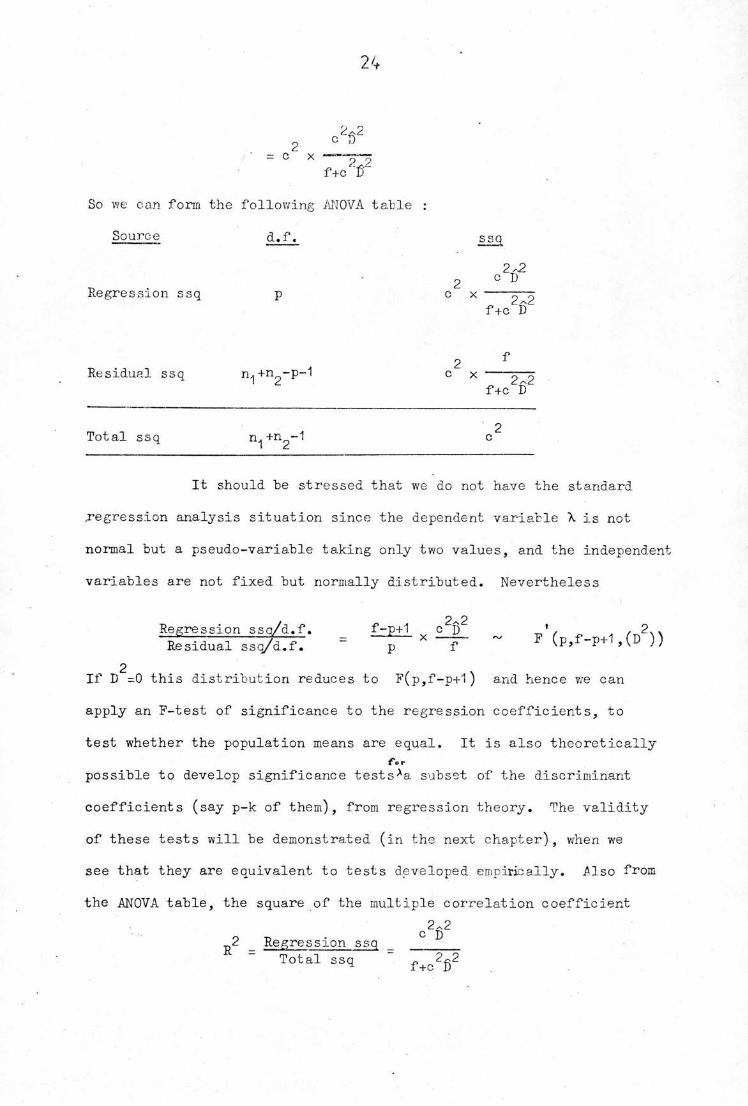
f+c¥So we can form the following ANOVA table

Source d.f. ssq

2-22 C

Regression ssq p c x • 2-2f+c D

2 **Residual ssq n^+n -p-1 c x

f+c D

2Total ssq +n -1 c

It should be stressed that we do not have the standard

.regression analysis situation since the dependent variable \ is not

normal but a pseudo-variable taking only two values, and the independent

variables are not fixed but normally distributed. Nevertheless

2/s2Regression sso/d.f.

_ £lE±l x £_JL „ f . /n2uResidual ssq/d.f. p f ^ ^ '

2 . ,If D =0 this distribution reduces to F(p,f-p+1) and hence we can

apply an F-test of significance to the regression coefficients, to

test whether the population means are equal. It is also theoreticallyfor

possible to develop significance testsâ subset of the discriminant

coefficients (say p-k of them), from regression theory. The validity

of these tests will be demonstrated (in the next chapter), when we

see that they are equivalent to tests developed empirically. Also from

the ANOVA table, the square of the multiple correlation coefficient2-2

o T> - CD2_ Regression ssqR =

Total ssq " f+c2fi2

2o

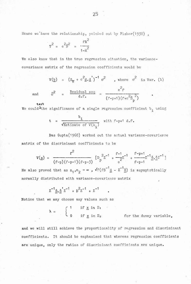
Hence we'have the relationship, pointed out "by Fisher(l938) ,

fR22~2

T - c 1) = '

1-R2

We also know that in the true regression situation, the variance-

covariance matrix of the regression coefficients would be

2 1 -1 2 2V(b) = (Syr + c d.d ) cr , where cr is V'ar. (X)

c2f^2 Residual ssq

ana o" = ~~d,f* " (f-p+i) (f+c2f)p2)

-test

We could^the significance of a single regression•coefficient b. usingi

b.t = -— 1 — with f-p+1 d.f.

"/Estimate of V(b.)x

Das &upta(l968) worked out the actual variance-covariance

matrix of the discriminant coefficients to be

f22 -1 f_1 -1 f~P+1 -1 -1

V(a) [D 2 + —xZ + 2 5.52 ](f-p)(f-p-1)(f-p-3) P c f-p-1

—1 —1He also proved that as n^ ,n^ -* 00 , Vf(fS d - 2 5) is asymptoticallynormally distributed with variance-covariance matrix

-1 ' -1 2 -1 -12 8.5 2 + D 2 + 2

Notice that we may choose any values such as

X =

r 1 if x in n t

i. 0 if x in n2 for the dummy variable,

and we will still achieve the proportionality of regression and discriminant

coefficients. It should be emphasised that whereas regression coefficients

are unique, only the ratios of discriminant coefficients are unique.

26

( S -8) HYPOTHESIS TESTING IN DISCEIMINANT ANALYSIS

For this section we need to introduce the following

partitioned vectors and matrices

d =

x(l) kft

5(1) k

x77)> _ -

p-k 8(2) p-k

d( 1 )" k

, 2 =E11 E12

d(2) p-k E21 E22

-1, a = 2 '5 =

a(l)

a(2)

k

p-k

p-k

S =S11 S12 k

S21 S22 p-k

i. E11 -2 ~E11 E12E22-1-1 -1

v v y22 "21 11-2 E22-1

where, 2,. = 2,, - 2 2-1.

J11 -2 11 12 22 21

J22-1 = S22 " Z21S11 S12 ' (See Morrison,p.68}

Now, from Kshirsagar(p.21),

-1 -1(I + LK) = I - L(l + ML) M - [6]

Thus '11-2 ~ E11 + E11 212E22-1221S11

= 2^ 1 + p 2,22.^/3 , where p = 2.,J21 11

Also 222 2^2^ >2- 7 2. f I - 2 ^2 £ S ) ^2 ^_ 222 i21U ^ 12 22 2V 11

- 2 -1Z 2 "1~

22-1 21 11

So we can write

,-1 Z11 "1 +",Z22->' -1

V-1~S22-P

-1

E22-1

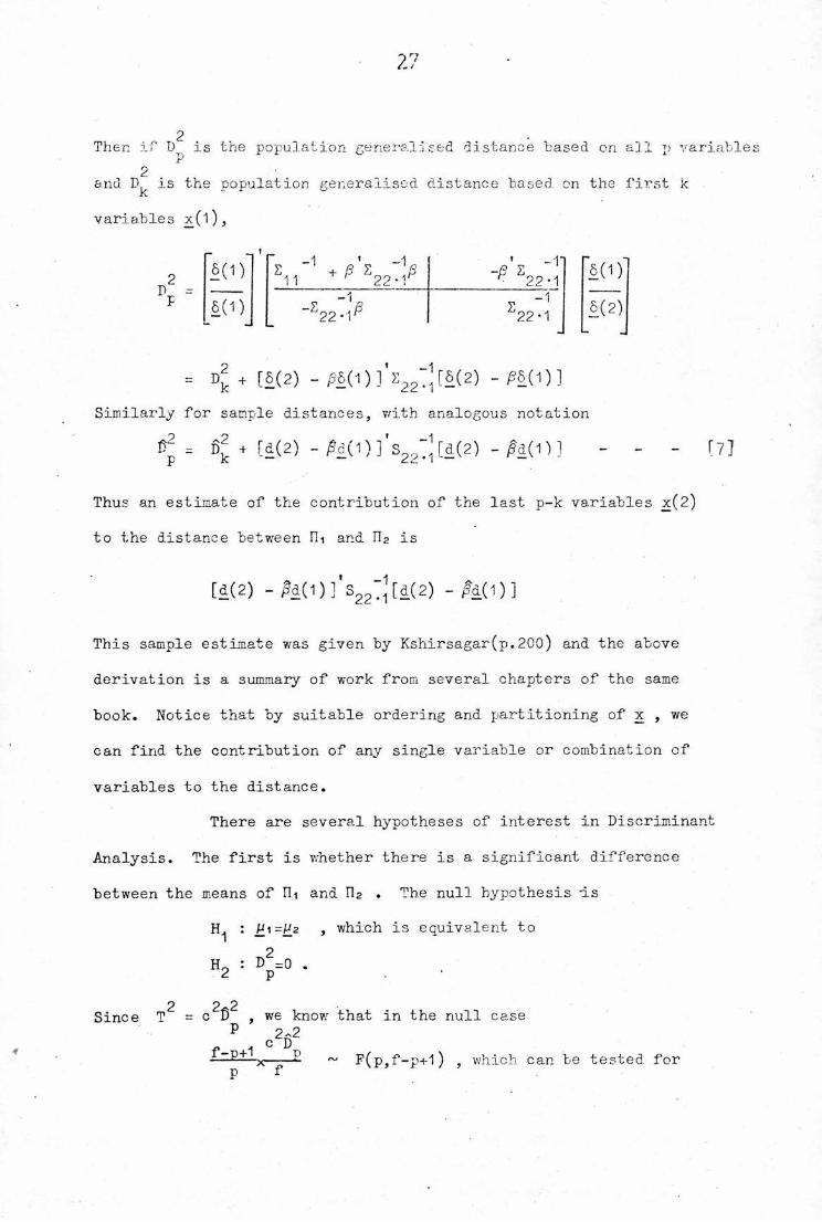
2Then if D is the population generalised distance based on ail p variable

r'2

and P is the population generalised distance based, on the first kK

variables x(l),

8(1)2

PF - 6(1)

-1 • -1

E11 V222-"Z22-> Z -1

22-1

"6(1)'6(2)

= [6(2) - /56(1)!,222:J[6(2) -/?6(1)]Similarly for sample distances, with analogous notation

Cp = - [d(2) -^d(l)]'s22;J[d(2) - - -

Thus an estimate of the contribution of the last p-k variables x(2)

to the distance between FW and U2 is

[7]

-1,[d(2) - /?d(l)j S ^ [d(2) - /3d(1 ) ]22

This sample estimate was given by Kshirsagar(p.200) and the above

derivation is a summary of work from several chapters of the same

book. Notice that by suitable ordering and partitioning of x , we

can find the contribution of any single variable or combination of

variables to the distance.

There are several hypotheses of interest in Discriminant

Analysis. The first is whether there is a significant difference

between the means of Hi and n2 . The null hypothesis -is

H-j : if1=£2 > which is equivalent toH2 : Dp=° *

2 2 2Since T = c f) , we know that in the null case

P 2-2. c D

—x P ~ F(p,f-p+l) , which can be tested for

28

significance in tables.

Secondly, we might ask the question whether the addition

of more variables to our discriminant function would significantly

increase its ability to separate n1 and Il2 . Our null hypothesis

here is

H3 • d,. . —Q.. —• • •

k+1 k+2..=a =0

P

i.e. H3 : a(2) = 0

Buta(l)

' -1"E22-1 ~5(1)"

a(2)_ ~S22-1/9

A

V 122-1

_

6(2)

Therefore, a(2) = 0 => S22 ^(5(2) -/SS(D) 0

i.e. 6(2) = ^6(1)

From [7], it is easy to see that a(2)=£ -> ^ 2D = D,

P kSo the hypothesis is equivalent to

2 2H, : D = D.4 p k

Rao(l965, p.482) gives the test for this hypothesis as

= F(p-k,f-p+l) -frEtl x °2(6' - $p-k „ 2-2 [8]

f + c D,

If this variance-ratio is not significant, the variables x(l) are

sufficient for discrimination between n1 and n2 . Obviously, by!

putting x(2)=x^ , x(1)= [x^ ,. .. ,x_. ^ »xp+-j»* • ,Xp- an<^ k=p-1 in [8],we can test to see if omission of x^ from the analysis significantlydecreases the effectiveness of the discriminant function. Incidentally,

Rao first gave this test in 1946 (see the list of references).

Thirdly, certain variates (known as concomitant or ancillary

variables) possibly have the same mean in both populations, thereby

possessing no discriminating power on their own. However, if they

are correlated with variables which do differ with respect to I11 and n2 ,

their inclusion may actually improve the discriminant function. Cochran

and Bliss(1 948) have pointed out that the analysis of concomitant

variables is analogous to Covariance Analysis. The null hypothesis of

interest when ancillary variates are present is

: 6(2) =0 given that 6_(1) = 02 2

or : D =0 given that D, = 0bp. k

2 2= D . = 0 given that D, = 0

p-k _ k

Since implies H. under the condition that 6(.1) = 0b 4 _

the F-test [8] is often used to test or IIg as well as or .

However, Rao(l949) suggested a test based on

v = 1(6I- t I).V

The statistic actually used is W = —- , with density

f(w) = [r(f+2k-p+i)r(£±l) / r(£^±l)r(k/2)r(£±E|bl)]k_1 f-P+1 1

X w2 (1 - w) 2

x F ( f'P+k+1 . f+k+1 w )2 1 2 3 2 9 2 9

where ^F^ is hypergeometric function of the second kind. Raopostulated that V was a better statistic than F[8] for testing ,

/s2since the variance of estimates of D he obtained based on F[8"l and V

P^2

given that D, = 0 , were smaller in the latter case. He also suggestedK

an approximate variance-ratio

f_p+1r f_k+1 ° (Du " V n

p_—[ ~f7T x t ] = Fp-k,f-P+i *

Fourthly, we want to test whether the linear discriminant

function we is sufficient to discriminate between Hi and n2 .

Our null hypothesis is!

: a given function y=h x is good enough to discriminate

between II-t and n2 .

~2Tc test this hypothesis, we apply the F-test [8] with replaced by

- — 2 '2" y2) (h d)

J) = = ;

Estimated Var. (y) h Sh

Thus if the variance-ratio

2,-^2 ~2.r_p+1 C ~ 1^

— x no— is significant, the linearP-1 f + c

t

discriminant h x is not the best discriminator.

Lastly, since discriminant function coefficients are

not unique, we cannot test an hypothesis of the form Pp~k * However,their ratios are unique and thus we can construct a null hypothesis

of the typea.

Hp : — = k .o a.

n-2 Îf D .is the generalised sample distance based on all variables

p-1

except xj \ > we can if k is the true value of the ratio usingX."

^ (jut + t<"X^

31

(f-p+1) X

2 / ^2 ^2 \

° <dp - °P-i)

p-i

i,f-p+i

This test is again due to Rao(l96p).

(1-9) SIZE AND SHAPE FACTORS

We conclude PART I , with a brief look at the special<na.tr i\

case, first considered by Penrose(1947) , when the dispersion*has the

form

2 . =

1 P.. .

P 1 P-. •

P..

P

P

PP 1

= (1 - p)l + e.<

Bartlett(1 951) showed that

-1e.e

1-p 1-p 1+P(p-1) , and consequently

' —1 ' *(Pi - P2) Z X oC[ —7- - £ ]x + [ p-1 ] £ x

e_ 6 1 +p(p-1)

Penrose called the two sets of coefficients, h and £ , the Shape

and Size Factors, respectively. These factors are uncorrelated and

hence independently distributed. It can be shown that the discriminant

function can be expressed in the form

—2 h x + —2 g x [9]

where 5^ is the difference in the means of the shape factor inn-t and n2 ,

and o; is the variance of the shape component. 6 and c~ areh g g

defined similarly. According to Bartlett, Penrose has shown that the

discriminant function [9] gives good results even when S is not exactly

of the required form. As such [9] has been successfully applied to

the analysis of biological organs, where size and shape are particularly

relevant.

3?.

PART II

(2-1) THE POPULATION DISCRIMINANT FUNCTION FOR PAIRED OBSERVATIONS

AND ITS DISTRIBUTION

Suppose our overall population n can be split into

Males(M) and Females(F), with equal prior probabilities of an individual

coming from either and equal costs of misclassification. 7/e introduce

the restriction that a new pair of observations (z^,z^) must be ofdifferent sexes i.e. only two cases can occur :

1) z, is Male, z„ is Female !~z,,<fM,z eF]' \ '2 12

2) z^ is Female, z^ is Male [zêF,zêM]It Is also assumed that z^,z^ are independent. No?/, if in the univariate

2 2case Males ~ N(hi,cr ) and Females ~ N(^2,cr ),

Prob. (zêMl there exist two pops. M and F , &/>JL no oi z*)1 (

exp —~2 (Z1 ~ Pi)=

12 1 2exp -—p (z-i""^0 + exp -—r (z(-/i2)

2cr 2cr

with similar formulae for the conditional probabilities that zêF,

zêMjZêF . Thus, using Bayes Theorem,

Prob. (z.j eM,Z2eF [ either case 1) or 2) must hold)

3 A

1 U \2 f ,2,exp r !(z,-pi) +(z -p2) ]

2a"

exp [(z -Pi)%(z -p2)2] + exp ~ [(?..-p2) + (s0-l'1)2'2a" * 2o *

1

1 + exp - ~2(Z2-Z1 )a

We will assign z.j->M,z2->F ^ >

i.e. if exp - ~2 (z2~z1)(^2~Pi) < 1cr

i.e. if (z1-z2)(pi-p2) > 0

Thus if we are given §=p1-P2 > 0 , we have a very simple assignment

procedure :

r If z, > z„ , allocate z .-»M,z -»FC j 2 2 [10]

If z, < z0 , allocate z.->F,z~->M12' 1 ' 2

Similarly, in the multivariate case, when Males ~ N^(pi,S), andFemales ~N^(£2,l) and we have a new pair of vector observations (z,-j ., z,2.) »

Prob. .fM,z_2>eF| one is Male, the other is Female)

f(£1l £1) x f C^21 ££2)• f (z^ 1^1 )x f(z2|p2) + fCzJps) x f(z2|pO

-1 1 -1 f= 1 / (1 + exp -g-tr. [2 (^-£2) (^.-£2) + 2 (z.2-£i ) (z.2""E1 )

~2 1 (£-] ~E1 ) (±.-5 -e0 - 2 1 (z2"E2 ) ( z2~E2 ) ^ )

= 1 / (1 + exp (^-£2) 2 ' (E2-E1 ) ) = P >

the obvious generalisation of the one-dimensional case,

35

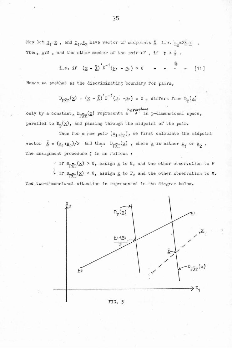
Now let _z,j ~x , and ,z_^ have vector of midpoints X i.e. z?=2X-xThen, xcM , and the other member of the pair eF , if p > r? ,

_ ' _ 1 V*i.e. if (x - X) 2 (p, - £2) > 0 - - - - [11]

Hence we seethat as the discriminating boundary for pairs,

^PXT(—) ~ ~ 2 1 ~~2^ = 0 ' differs from Dr,,(x)

only by a constant, D - (x) represents a A in p-dimensional space,I AI

parallel to D^Cx), and passing through the midpoint of the pair.Thus for a new pair (z^ ,z_0) , we first calculate the midpoint

vector X = (z,+.z9)/2 and then D - (x) , where x is either z_ or z .I C. * i.A.i i rd

The assignment procedure £ is as follows :

^ If D - (x) > 0, assign x to M, and the other observation to Fr Ai

If D—^x) < 0, assign x to F, and the other observation to Iff.rAl

The two-dimensional situation is represented in the diagram below.

Next we consider- the distribution of D - (x). When xcM ,Jta l

x - X ~ N ( (D1-P2)/2 , S/2) , so that_ _

p _ -

E[DpxT (—) ] = ~~z) S" '(H1-£2)/2 = 152/2Also Var.[Dp-T(x) ] = (£i-£z) 2~1SS 1(£t-£a) = D2/2

Thus if xeM , Dp-p(x) ~N(D2/2,DZ/2)Similarly if xeF , Dp-T(x) ~ N(-D2/2,dV2)

(2*2) THE SAMPLE DISCRIMINANT FUNCTION FOR PAIRED OBSERVATIONS

AND ITS DISTRIBUTION

We shall discuss two criteria for dealing with the situation

when the parameters of the Male and Female distributions are unknown.

The first is analogous to the criterion of (1*4), and the second is

the likelihood ratio criterion. This chapter is only concerned with

the first of these.

Taking samples of size m from the Male population and n from

the Females, we calculate X-j > —p an<^ samP^-e nieans and pooledsample dispersion matrix, as defined in PART I. Then substitution in

D^YTiCi) giyes us (x), the sample discriminant function for pairs,rAl x.Ao

where

dpxs(~) = ~ 2.) - E?) .

The unconditional distribution of D - (x) is not normal. However,x ao

if , we see that from the independence of S and (x^ - x ),

E[Dp^s(x)] - E[x - X]'e[S~1 jEt^ - £2]

37

Now, Das G-upta(l968) has shown that if S ~ V<r(2,n,p) ,

E[S_1] = ~~r S"1n-p-1

= J5±Sz^ b2/2m+n-p-p

= m+n~2 E[D - (x) ]ra+n-p-3 L PXTV-/J

Hence, even under normality, the coefficients of x in D - (x) are1 AO

biased for the coefficients of x in D_^^,(x). But, we have seen inX" Jv_L

PAKF I that discriminant functions, in general, are unaffected by

scale changes, and so the factor m+n is of no importance.m+n-p-3

If x^M , D™ (x) is conditionally normally distributedIT.A.O

with mean

E[Bp-s(x) ] =!(£, - £2) S"1^ - x2)and variance

Var. [Ep^g(i) ] =^(i1 - i2) S-V1^ ~ i2)where the expectations are conditional on x.] > —2 an<^ canfind similar expressions when xfF . Our estimated allocation rule is

* r If D_r: (x) > 0, assign x->M , other individual ->FC j FXS

If Dp^g(x) < 0? assign x->F , other individual ->M .

Notice that since D - (x) is parallel to the sampleIAO

discriminant function for classifying single observations, the regression

analogy (and consequently all the work of (1*7)) still holds for pairs.

We may also apply the hypothesis tests of (1 -8) to the coefficients

of Dp^ (x) , and the theor3r of size and shape factors can be easilyIAD

38

modified. Replace x "by in [9] to get

2ex cr

This simplified discriminant function may have particular relevance

to the sexing of pairs when we discriminate on the hasis of certain

organs e.g. wing, beak. Since the above function reduces to the sample

discriminant function in the bivariate case, we were not able to apply

it to to the fulmar data.

(2-3) THE PROBABILITY OF MISCLASSIFICATION

Define to be the probability of misallocating

a randomly chosen pair, eM , , using £ . Letting x=z<| , wes60 "fchsi/fc

= f(-D//2)

Similarly, a2(£) = §(-D/"/2)*

We also define ai(£ ) to be the conditional probability of misallocating. *

the pair (z^ =xeM , z^F) when £ is used. Then

°i(c) = Prob. (Dp^T(2S) < °l 2£eM and

«,(C') = Prob. (Pp^gCx) < °f 2£eM^2eF'-1'-2 and S'x ' -1 ,

*

Similarly for a2(£ ) .

It is suggested that a-i(£ ) may be estimated "by most of the methods

outlined in (1 *6) . Okamoto's expansion will have to be adapted but

the 6 method, for instance, will yield the estimate

«,(£*) = §(-fi//2)

We now describe the modified U Method in more detail. Having omitted

one Male and one Female sample vector, we classify the pair they form

using the paired sample discriminant function estimated from the

remaining m+n-2 observations. The procedure^by successive omission

of each possible pair of Male and Female from the sample matrices

X1 (Males) and X^Females) .

It can easily be seen that the pooled sample covariance

matrix when x. is omitted from X, and x. from X„ , is given by-x 1 -j 2

_ m+n-2 „ m ' n u ,Qu(ij) m+n-4 (m-1 ) (f-i.) —i1—i1 (n-l)(f-l) J

where u.. = x.-x , u = x.-x~x1 -x -1 -jA -j ~2

I mNow if

(i) ' = Jl2 S ~ (m-1 ) (f-X)m

-ii-xi }

S(ij) S(i)' (n-i)(f-t) "J2~j2

Hence, using Bartlett's matrix inversion

S/ "J _ s "I + °2S(ibai2-i2SfiVs(u) - s(i)' M . c u's,f 2~j2 (i) j2

where

Z,0

5(i) ^[s-1 ci3 -ii-iis- C u 3 u.,1—1.1 -x1

m, n

c„ — / . \ r-4 ana c — / , \ _ a1 (m-1)f 2 (n-i)f

Thus in the paired case, we still only require one specific matrix

inversion - that of S. If d,.. N is the difference between the sample~Uj)means of the remaining m+n-2 observations, it can be shown that

u.u ~

d, , = a - tVxj/ — m-1 n-1

The paired sample discriminant function computed without x. and x. isJ

-1

h/xW -Cil -iz) 8(J)i(ij) .

which can be legitimately used to classify the pair (x.,x.) • Thus,J

we see that the pair (x.,x.) will be misclassified ifJ

f -1D. . (x.,x.) = (x. -x.) S/..N d/..x < 0

_ -j) -(ij)ij "x ~J

The process is repeated for all the mn possible pairs from M and F ,

and the proportion misallocated is recorded as 6.£

Defining C . ,,x ) bym-1 .n-1 x ,1

rA (x.,x.m-1,n-1 i j

"J

r = 1 if (x.,x.) is misallocated1 J

^ 0 otherwise ,

_m pi

e E)M

mxn

, * V

Thus 6 is exactly unbiased for a, (£ A ) and approximatelyJ m-1,n-1 ^ Junbiased for at) , where the notation is the same as in (l'6) .

The method is <xn /*«.«t" upc.\ the U Method for single observation*

since we average over inn £ values as opposed to m+n in the standard

method. Consequently, the modified U Method should provide very good

estimates of paired misclassification probabilities.

Notice that since --D/V2 < -D/.2 , §(-D/vr2) < §(-D/ 2) ,

the probability of misclassification 1'or adding a single observation

i.e. we are less likely to make a misclassification error when we

allocate a pair of observations, under the conditions of (2*1), than

than when a single observation is sexed. Thus if two individuals are

known to be a pair, the extra information imparted by this knowledge

leads to a distinct improvement in their chances of being classified

correctly. . , , ,• ,it/itk fteyaa LThe univariate caseîs now considered in more detail

the assignment procedure £ has already been given in [10]. Suppose

z1 ~ N(pi ,<x2) ->2 | independently ,

z2 ~ N(p2,cr ) J2

then z - z^ ~ N(pi-p2 ,2cr ) ,

and a,(£) = Prob.(z -z <o| zêM , z eF) = §(-5/72),

where 5=pi-p2/cr . We now take samples (x^ ,... ,x^ ) from M and\ ^

(x10,... 5xno) f>ron an<3- estimate £ by £ which says

• if (x.-x )(z -z ) > 0 assign z„->M , z ->F_1 _2 1 2 1 2 [12]t if (xrx2)(zrz2) < 0 , assign z^F , z^M .

r Prob. (z >z ) if x <xr«i(0 = . J 12 _1 _2I Prob. (z1<z2) if x1>x2

1 - $(^2-Pi/cr/2) if x <x

1 - $(p1 -P2/0V2) if x1 >X,

12 r i[a J

— 2 — 2Now x.. ~ N(î,cr /n) independently of x2 ~ N(/i2,o" /n) .

— - 2So x-]-X2 ~ ~^2 >2°" /n) « and averaging over all possible

samples (x.^ ,.. . 'xn-|) from M and (x , ... >xn2^ from P, we obtain

p[ai(£ )] = $(6/vr2) §(-6Vn/vr2) + §(-6//2)$(8Vn/V2)

= the unconditional probability of misallocation

If we- now substitute the estimates x^ , x2 and s for p'1 , Ne and crin [a], we get

°i(s*) =

VxisV"2

r1 _ §( -2-1 ) < x2

x -x

1 - 1 ) x1 > x2s/2

= 1 - §( [81/V2)n""i

whe re 6 =irs2 2 ) + KrV2

, s =

2(n-l)

To calculate Efai(^ )] , let cr - A . Then*

VX2 „ „ V*2E[a,(C )] - Prob. ( ~f2~ < 0 and X < )

x.-x X.-X

+ Prob. ( --J2 >0 and- x> )2 ^ '

43

where X'~ N(0,1), independently of x,,x and the expectation is everI eL

all possible samples size n from I,'and F .

* X1"X? , X-"X'xTherefore, E[ai(£ )] = Prob. ( —7^— < 0 ) + Prcb. ( -X + —77, ~~ < 0)

_ 2xProb. ( V!i < 0 and _x + Vf2 < 0}

But ^ „ N( Pi^ ^ l/n }

o ^ V X1 "X2 ^ TcrC Pi -Pa „ 1 \ru ^ + y*2 ^ v~2 ' ' + n

Therefore, E[Si(£ )] = §(-5vn/vr2) + 5(-5/n/V2(n+1 ))- 2$(-5vrn/vr2 , ~6Vn/V2(n+1) ; p)

where $(a,b;p) is the bivariate cumulative normal distribution with

correlation p .

Now E[(-X + ^)(^)] = iE[(5rx2)2]1-i 2

= — + 'g'Cpi-pa) , and after a little

algebra it is easily seen that

p = 1/Vn+1

The table below shows

1) The true probability of misclassifieation using C, °i(t)

2) The unconditional prob. of misclassification using £ , E[ai(£ )]

3) The expected value of the estimated prob. of misclassification,

E^CC*)!.Assuming M ~ N(pi,1) , F ~ N(p2,1) , l)>2) and 3) have been calculated

a

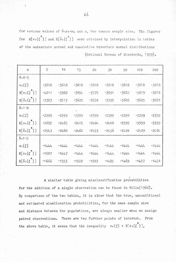
for various values of S-pi-jU2 and n, the common sample size. The figures

for E[ai(£ )] and E[Si(£ )] were obtained by interpolation in tables

of the univariate normal and cumulative bivariate normal distributions

(National Bureau of Standards, 1959).

n 5 10 15 20 30 50 100 200

6=0 *5

<*i(0 •3618 •3618 •3618 •3618 •3618 •3618 •3618 •3618

E[«i(C )] •4211 •3982 •3854 •3775 •3691 •3622 ■3619 •3618

E[Si(c')] •3323 •3517 •3622 •3650 •3595 •3608 •3625 •3622

6=1 -0

«i(0 •2399 •2399 •2399 •2399 •2399 •2399 •2399 •2399

E[«I(C )] •2695 •2465 T—-4"C\J •2404 •2400 •2399 •2399 •2399

E[ai(C )] •2543 •2480 •2462 •2453 •2436 •2420 •2409 •2404

6=1 "5

«1 (c)

E[«i(£*)]E[Si(OJ

•1444 •1444 •1444 •1444 •1144 •1444 •144+ •144

•1507 •1447 •1444 • 1444 •1444 •1444 •U44 ■ 1444

•1666 •1553 •1522 •1503 •1485 •1469 •1457 • 1450

A similar table giving misclassification probabilities

for the addition of a single observation can be found in Hills(l966).

By comparison of the two tables, it is clear that the true, unconditional

and estimated misallocation probabilities, for the same sample size

and distance between the populations, are always smaller when we assign

paired observations. There are two further points of interest. From$

the above table, it seems that the inequality «i(C) < E(ai(£ )],

/> 5

hypothesised by Hills for single observations, still holds for pairs.*

/s *Secondly, the approximation )-«i(C)]=0, which was good

in Hills' paper, no longer seems appropriate for pairs, even when

sample sizes are large. This might indicate that the D Method does

not yield very good estimates of paired misclassification probabilities.

Further research needs to be carried out into the relative merits of

all the estimation techniques when they are applied to pairs ; sampling

experiments should be performed on the lines of Lachenbruch and Micke\r's

(1968).- ^ *

Incidentally, it appears that Hills' formula for E|_Qi(£ )J

is incorrect and should be, in his notation,

E[Si(£*)] = G(-a) + G(-b) -'2G(-a,-b;p ) .

It was then thought that an improvement in the magnitude

of the misclassification probabilitiesAif the allocated pair (z^,z9)were used in the formation of a new discriminant rule , where

- if (z -z) ) (x -x ))o assign z -»M , z ->F=> |

if (z^-z^) (x^ -x^)co assign Zy>F , z^->M

where x^ is the new estimate of Pi from the n+1 sample values(x. x „) together with either z. or z„ . Obviously,v 11 ' ' n1 1 2

Bl(0 = 1 - §(8//2) , still.

r if x'< x*„ fr*\ f 11 X1 2

L 1 - *("57T) ■ X1> X2

But Prob. (x < x ) = Prob. (ri^+z^ rn^+zÔ^ zjlx^ xjjz^ > 593)

+ Prob. (mq+2^ nx2+zj^\[z^< zjlx^ x^z^ > zo0x1 > x^)

£6

= Prob. (z„> z/lx < x„) i- Prob. (z < z fix > x )i £ i 2 i 2 i 2

= Prob. (x,< x2)3{l r

Thus E[ai(£2)] ~ )] 5 an(t there vri.ll be no gain in informationif the unknown pair (z^,z ) is included with the original sample data,to form a new allocation procedure for the sexing of subsequent unknown

pairs.

(2-4) THE LIKELIHOOD RATIO CRITERION EOR THE CLASSIFICATION OF ONE

NEW PAIR (UNIVARIATE)

In this chapter, we consider the application of the

likelihood ratio criterion in the formation of population and sample

discriminant functions for classifying paired observations. Firstly,

in the univariate normal case with known parameters,1 1 ,2

the Male p.d.f. is ^(x) = V2ircr ex^ ~ —22cr

1 12and the Female p.d.f. is f-„(x) = fn exp - —- (x-^z)F

2a

The likelihood of the new pair (z^,z^) being (M,F) is

2 1 2 2f/2rrcr x exp - —^ [ (z -Pi) + (z^-Pz) ] ,

2o

and the likelihood of it being (F,M) is

2 1 2 21/27TCT X exp - —2 [ (z-,-^2) + (Zp-Ui) ] .

2o"

But, from PART I , we know that the discriminating boundary is given

by the likelihood ratio (L.R.) = 1 and

12 22 22 22L.R. = exp-—p[z -2z +z/"-2z p2+p2 ~z +2z./j2-/j2 -z

2a ^ ^ ii 2+2z ]

log(L.R.) = (z1~z2) (pi-p2)/cr2 .

Thus our discriminating boundary is (z^-z )(hi-^2) = 0 which leadsto the same rule, £, as [10] . £ will now be referred to as the L.R.

❖

rule. Obviously, £ is the estimated L.R. rule.

When the population parameters are unknown, we take samples

Cj 1 j • • •11 mi

2xn'-*- >x^ ~K(pi,o'") from M

2and x. ,x ~ N(/u2,a ) from F12 n2

Denote the hypothesis that (zj,z- ) is (M,F) by , andthe hypothesis that (2 ,z ) is (F,M) by H .

I C. \J

Then, under , the likelihood of obtaining the samples

x^ j. .. , x ^ from Mand x_j2,... >xn2 *>rom proportional to

11 = l/oJn+n 2 exp—^[2(x-j-Vi)2 + £(x.2-h2)2 + (z.-î)2 + (z -IJZ)2]2a

-1 m+n+2 _2 1 rs/ \2 «, \2 , x2L1 = log 11 g— loS a ~ —2^ (xil"A'1) + ^^xi2~^2 +

2a"

+ (z2-p2) "]

The maximum likelihood estimates of Pi,p2 and cr2 , under , are

given by setting their partial derivatives with respect to L^ equalto zero. Thus

mx,+z. nx +zQ — —J L u — - —

11 ' 21,m+1 n+1

L'6

ana °-| - m+n+2 f + ^(x-j_2~^z 1 ^ + (z-j-h-ii) + (Z2"'J21) 1

/\ /\ /n 2 2where P-m, h'ai and <x^ " are the M.L.E.'s of hi,/J2 and cr under H.

Substitution of these M.L.E.'s in =>

m+n+2 ~ 2 m+n+2L log cr - —

Similarly, under the alternative hypothesis

mx^ +z2 nx„+z,h 1 O = , h 20 -

m+1 n+1

/s2 1 r ^ \2 Â 12 f ,2 . >2 ,

°0 = M+2 ^ ^xi1^1°) + 2^xi2"^20^ + (Z-T^20) + vz2-Pio) ]

... c m+n+2 a 2 m+n+2Also Lq = - -y- log o-Q - -T-

*• c .m+n+2 , a 2 2Thus L1 > Lq if —-— log crQ /o^ > 0

- 2 - 2i.e. if crQ >

i.e. if 2(x^-£io)^ + Z(x^-p2o)^ + {z^-Pzo)^ + (zp-Pio) >

SCx^-Pll)2 + 2(*i2-h2l)2 + (zr/Jll)2 + (z2-Pzi )2which, on substitution of the M.L.E.'s, gives us

2 2—2 — 2(mS^+Zg) (nx2+z1) (mx^z^ (nx2+z2) _ (z2~zJ! + _ _ 2mx^— :—

m+1 n+1 m+1 n+1 m+1

1*9

_ (zo-zi) (nx +z ) (ax,+zj (mx +z )+ 2nx2 2 7^ 2z? + 2z1

n-h1 n+1 " m-t 1 m+1

„ (n-VZ2)+ 2z > 0

n+1

This inequality simplifies to

(z1-z2)[(n-m)(zJj+z2) + 2m(n+1 )x.; - 2n(m+l)x2] > 0 ,

Thus, in the univariate situation, we have the following assignment

procedure, rj, for the pair (z^,z )

r If > 0 assign z-f>M , z^FIf DpLS^z-i'Z2^ < 0 assign z^F , z2->"

win 're DPLS^Z1 'Z2^ = (zi~z2^^n~m^zl+z2^ + 2=l(n+1)x1 " 2n(m+1 )x2]

Notice that if the sample sizes are the same i.e. n=m , y) reduces to

the estimated L.R. rule for paired observations, £ (see [12]). The

unconditional distribution of D (z., ,z ) is complicated and noriLiS ' 2

attempt has been made to evaluate it. However, we can look at its

expected value.2 2 2

Suppose z^ eM , z^F. Then, E[z^ J = Pi + <r and2-, 2 2

E[z2 ] = p2 + cr . Then, taking .. expected values over allsamples (x^,... »xm1Jz-,) fnom M and (x^,... >xn2'z2^ from F>

2 2

E[DpLs(V22)] = (n-m)(pi -p2 ) + (pi -p2) [2m(n+1 ^ - 2n(m-2

= [m(n+l) + n(m+1)](Pi-p2)^

= [m(n+1) + n(m+l)]S[DpT(z1,z2)] ,

50

where Dpp(zrz2) - Oj-^KUi ~Vz)

Therefore, the coefficients of z, ,2„ in D^„ „(z. ,zn) are biased.1* 2 PnS 1 2'

for the coefficients of z-pz2 z-j >once more usingthe fact that scale changes do not affect allocation procedures, we

see that ^ppg(z-]'z2} ^"s rea^l 'unbiased' for D^(z^ , z^).

(2-5) THE LIKELIHOOD RATIO CRITERION FOR THE ADDITION 0? TWO NEW PAIRS

(UNIVARIATE)

In practice.we may observe several new pairs and require

to allocate them as a whole. Ideally, for the the purposes of practical

discrimination, when all the new pairs have been introduced, the rule

would break down into the independent assignment of each pair.

Suppose we have two new pairs (z^z^) and (w^,w2), andthe usual samples size m from M , n from F . Then, since there are

four different ways of allocating the two pairs, we have to consider

four hypotheses. They are :

1) H1 : (z^MjZ^F) and (w^MjW^F)By the obvious extension of the previous case, the M.L.E.'s under H^ are

mx.+z.+w. nx +z +wn 111 ^ 2 2 2P11 = , /i21 ,

m+2 n+2

^ 2 1 r Q f ~ v 2 H / A * 2 t ,2 f avv2 / ^

a1 " rn+n+4 ^ + 2(xi2-U2i) + (Zl-Pn) + (z2-/j£i) + (w^Cti( A \ ^ i+ \.w2-/i2i) J .

<> m+n+4 t ~ 2 m+n+4Also, o1 = - —J— logecr - -5-

51

2) H2 : (z^MjZ2e?) and (wêFêM)3) : (z1eF,z2eM) and (w^MêF)4) : (z1eF,z2eM) ana (w^FêM)

The M.L.E.'s and log likelihoods under H2,H^ and are similar tothose under . We will have independent assignment of the pairs

if £„-L2 leads to the same procedure as L -L. , and L-L_ leadsI j 2 4 12

A A

to the same procedure as L^-L^ .

A A 2 A 2Now -£^ >0 if o_ > 6^ . After a little algebra,

it can be shown that

> ° lf (zi~z2^^n_in)(zi+z2^ + 2(n+2)(w1+mx1) ~ 2(m+2)(w2+nx2) J> 0 .

■By symmetry, f^-l, > 0 if

(z^-z2)[(n-m)(z^+z2) + 2(n+2)(w2+mx,j) - 2(m+2)(v^ +nx2)] > 0 .

Therefore, we cannot reduce the allocation procedure for two new pairs

into their independent assignment (except in the trivial case of w^=w2 ,

or z^=z2). It is worth noting that the situation might arise in practicewhereby we know (z^,z2),(w^,w2) are either (M,F),(M,F) or (F,M),(F,M),For instance, a biologist may have classified some observations using

a common coaÂa. that the first individual in a bracket belongs to

one group, and the second belongs to the other group ; a second biologist

looking at the data may not be able to tell which way round the pairs

are. For this problem, we need to compare with H, . After moreA A

algebra, it can be shown that if

(z1-z2)[(n-m)(z1+z2) + 2(n+2)mx1 - 2(m+2)nx2] - 2(n-m)(z1w1 + z^)+ (w1-w2)[(n-m)'(w1 +w2) + 2.(n+2)mx>| -2(m+2)nx2"' > 0

COi-

Hence the second biologist will be able to come to a decision as to

whether the notation used was (M,F),(M,F) or (F,M),(F,M) .

We can extend the analysis to the addition of k new pairs

(z.„,z ) (i=1,... ,k), when we vri.ll have to choose between 2^ differentv i1 i2

hypotheses. A search procedure should be introduced to shorten trie

number of computations required (maximum of 2 likelihoods). Two

algorithms are suggested for the bivariate case in (2-12), where their

application to the Fulmar data is discussed.

(2-6) THE ALLOCATION OF A SINGLE OBSERVATION BY THE LIKELIHOOD RATIO

CRITERION (UNIVARIATE)

Suppose the new individual is w and we have the usual

samples from M and F. From Anderson's (15§$) multivariate result,

a little algebra leads us to the conclusion, that we assign w->M if

2 — — — 2 — 9

DLg(w) = (n-m)w - 2w[(m+l)nx2 - (n+l)mx^] + (m+l)nx2 - (n+l)mXj > 0 [ 13]

Putting n=m in [13], we see that w is assigned to M if

î+x2(x -x ) (w - — ) >0 , which is the same rule as f5 I.

2

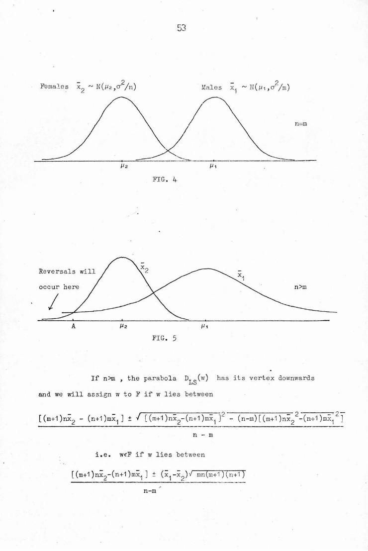
If n/m , there will be cases of reversal. The diagrams belcw illustrate

how the discrimination rules depend on the sample sizes.

In FIG-, k we see that the sample means x^ ,x2 have thesame distribution (with different means), and the cut-off point is

simply (x^+x2)/2 . FIG. 5 shows how, when n>m and consequently2 2

cr /m > cr /n , reversals will occur to the left of the point A .

— 2 — 2Females x^ ~N(p2,cr /n) Males x^ ~K(jUi,cr /m)

FIG. 4

FIG. 5

If n>m , the parabola D (w) has its vertex downwardsLS

and we will assign w to F if w lies between

_ _ — —— 2 — 2 ^~~r 2~~[(m+l)nx2 - (n+1 )mx^ ] + v [ (m+1 )nx,_,-(n+1 )mx^ ] - (n-rn) [ (m+1 )nx,-, -(n+1 )mx^ ]

n - m

i.e. weF if w lies between

[ (m+1 )nxp-(n+1 )mx^ ] ± (x^-x )V mn(m+1)(n+1)n-m

5^

If we are given weM ,

O

E[D (w) ] = (n-m)hi - 2 I" (m+1 )nH2--(n+1 )mhi ]Lb

+ (ra+1 )n(^2^+o"^/n) - (n+1 )m(pi ^+0"2/m) + (n-m)cr22

= (m+1 )n(hi -p2)

= 2(m+l)nE[DT(w)]2

Similarly, if weF , E[D (w) ] = (n+1)m(hi-p2)iJO

(2*7) THE PROCEDURE FOR POPULATIONS WITH EQUAL MEANS AND UNEQUAL

VARIANCES

2 2Suppose M ~ N(p,o~i ) and F ~ N(r,ct2 ) , and we have

to classify the new pair (z^,z^) . The probability of (z.j,z ) being(M,F) is

1 / n2 1 , v

—(Zl-h) - -(z^-p)1 1 / n2 1 , n2

~2—2 eXp27ro-1 cr2 2Cm 2ct2

and of being (F,M) is

L— exp _ -~(z n)2 _ —!_( p)22770-10-2 2o-, 2O-2

Putting the logarithm of the L.R. equal to zero, we find our discriminating

boundary to be2 2 Z1+Z2

(v5^) (°"1 -°~2 )( 2 " H) = o •

When the population parameters are unknown, we take the usual samples

from M and F, and form two hypotheses :

1) H. : {Zj[ ,z2) - (M,F) . Under ^

<?2?(mx.j +2 . ) + a,f(nx +zQ)^1 - - ~ - —

(ra+l)5"2i + (n+1 )*i?

<Ti? = [ Z(xi1-/î)2 + (z^Pi)2 ]/(m+1) , 5"22 = [2(xi2-/Ji)2 + (s2-£i)2]/(n+l)

, a. m+1 , ~ 2 n+1 , ^2 1,and L1 = - log^cru - —— log^cr^ - ^{m+n+2)

2) Hg : (z.j ,£?) = (F,M) . The M.L.E.'s and Hog L.R. under are

similar to those under .

We choose in preference to , if L^-L^ > 0

• j> m+1 a 2 /<-. 2 n+1 ^ 2 2i.e. if ——log CTio/CTn + —j-log O2o/O"2 1 > 0

i.e. if

a 2 m+1 a 2 n+1

*T©T • •- 2

Similarly, it can be shown that we classify a single observation w as M ifav 2 m a 2 n

2 f \ 2 5-2o^ •*:— > 1 , where tne M.L.E.'s are2 / , '1 /

given by similar expressions to the M.L.E.'s under the two hypotheses,

in the paired case.

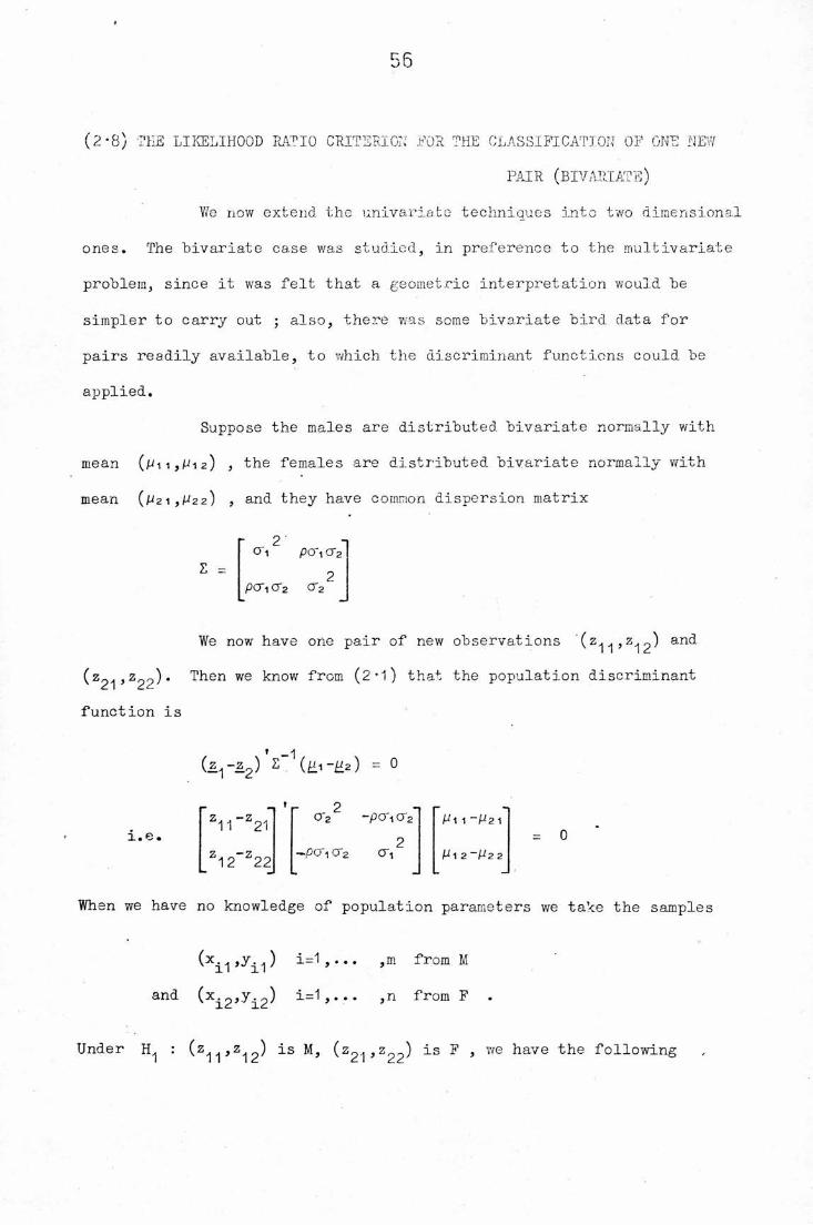
(2-8) THE LIKELIHOOD RATIO CRITERION FOR THE CLASSIFICATION OF ONE NEW

PAIR (BIVARIATE)

We now extend the univariate techniques into two dimensional

ones. The bivariate case was studied, in preference to the multivariate

problem, since it was felt that a geometric interpretation would be

simpler to carry out ; also, there was some bivariate bird data for

pairs readily available, to which the discriminant functions could be

applied.

Suppose the males are distributed bivariate normally with

mean (pi 1,^12) , the females are distributed bivariate normally with

mean (^21,^22) , and they have common dispersion matrix

Z =

2cr 1 po"1 cr2

P<J~1 0~2 0*2

We now have one pair of new observations (z-|-i>zi2^ an(^

^Z21'Z22^* ên we know from (2*1) that the population discriminantfunction is

2 = 0

i.e.Z11"Z21

Z12_Z22

cy2 ~po~1 o 2

2-po-, cr2 cr1

U1121

N12"P22

= 0

When we have no knowledge of population parameters we take the samples

(Silî-,) ,m from Mand (xi2'-î2^ i=1 > • • • >n from F

Under : (z-|-] > z-j 2^ (Z21'Z22^ as ^ ' we âve ^he Following

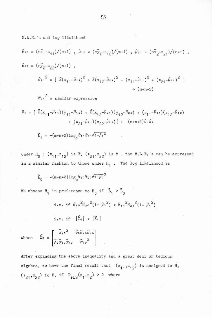
M.L.E.'s ana log likelihood

P11 - (mx1+z11)/(m+l) , pi 2 = (my1+z12)/(m+l) , p2 1 = (nx2+z21 )/'(n+1) ,

P?2 = (ny2+z22)/(n+1) ,

^1|2 = [ 2(xi1-Pii)2 + Z(xi2-p2i)2 + (z^-Pn)2 + (z21-P2i)2 ]-T- (m+n+2)

a 2 .

0b 1 = similar expression

Pi = [ 2(xi1-Pn)(yi1-Pi2) + S(x.2-P2i)(yi2-P22) + (z11 -Pi 1) ( z1 2~Pi 2)+ (z21-p2i)(z22-p22) ] -r (m+n+2)a16L2

= -(ni+n+2)log o"i i<x2 i/T-pT2

Under Hq : (z^jZ^) is F, (Z2i»Z22^ ^"S ^ M.L.E.'s can be expressedin a similar fashion to those under . The log likelihood is

yv / 2Ln = -(m+n+2)log <Xi ocr2oV1 -p oU G

A A

We choose H. in preference to H„ if L. > L„1 c 0 10

• * r* A 2/. A 2\ a 2 2/. A, 2.i.e. if oi o O"2o (1-Po ) > cTi i cr2i (1- pi )

where So =

i.e. if |So| > |SiA 2 A A Acr1 o Pocr i ocr2o

A A - 2P0CX1 ocr2o cr2o

After expanding the above inequality and a great deal of tedious

algebra, we have the final result that (z-|-|>z-)2^ ^~s ass^-Sne(^ "to

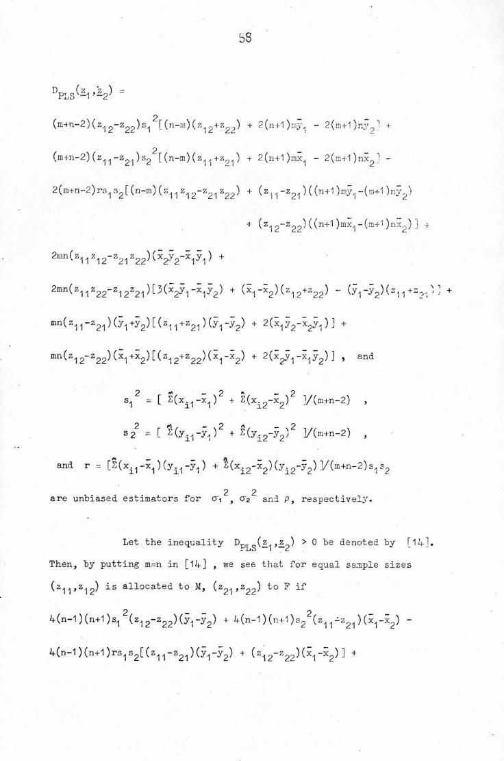
(Z2i'z22) to F> if DPLS^-1'~2^ > ° Wh6re

b8

2 - __

(m+n-2)(z12-z22)s1 [ (n-in) (2+z?2) + 2(n+l)my1 - 2(m+l)ny9l +

2 - -

(m+n-2)(z^-z2j)s2 [(n-m)(z^1+z91) + 2(n+l)mx1 - 2(m+l)nx2] -

2(m+n-2)rs1 s2[ (n-m) (z^ z1 2~z21 z22) + (z^-z^ ) ( (n+1 )my.) -(m+1 )ny2)

+ (z12-z22)((n+l)mx1-(ra+i)nx2)j +

2<m(zu',2-z2^22)(x^2-x^) *

2mn(z11z22-z12z21)[3(x2y1-x1y2) + (*-,-*2)(z12+z22) ~ (yn-y2)(211+22V( J +

mn^z11_Z21^y1+y2^('Z11+Z21^yry2^ + 2^ly2"x2y1^ +

mn(z12-z22)(x1+x2)[(z12+z22)(x1-x2) + 2(x^-x^)] , and

s.j2 — [ ^(x^-x^2 + E(xi2-x2)2 ]/(m+n-2) ,

s 2 = [ + 2(yi2-y2^2 ]/(m+n-2) ,

and r = [S(x±1 -x1)(y±1-y.,) + 2(x±2-x2)(y±2-y2)]/(m+n-2)s1s22 2

are unbiased estimators for o~i , cr2 and P, respectively.

Let the inequality Dw (z ,z„) > 0 be denoted by [14].rIjo 12

Then, by putting m=n in [14] , we see that for equal sample sizes

(z11}z12) is allocated to M, (z21>z22) to F if2 - - 2 - -4(n-1) (n+1 )sJ| (z12-z22)(y1-y2) + 4(n-1 ) (n+1 )s2 (Z11-z21 ) (x1-x2) -

4(n-l)(n+l)rs1s2[(z11-z21)(y1-y2) + (z^2~z22)(£,-x2)] +

59

2n(z11Z12"221ii22)(;^2-i^1) +

2n(z11Z22"Z12Z21^3(X2y1~X1 y2> + (X1"^2^Z12+Z22^ " ^y1 ~y2^Z11+Z21 ^

n^Z1l"Z21^y1+y2^^Z11+Z21^y1~y2^ 2(^y2~x2y1^ +

n(z12~z22)(x1+x2)[(z12+z22)(x-|-x2) + 2(x2y1 ~X1y2' ^ > [15]

L, > L„ if1 0

Letting m,n-><» in [14] , it is clear that in the limit

2 2

^-(Z1 2_z22â". (^12~^22) + ^"(Z11 -Z21 ^CT'2 (^11~^21)

- 4pcricra[(z11-221)(î2-/i22) + (z12-a22)(/in-#i2i)l > 0

i.e. if2 2, 2.

cri or2 (1-p )

Z1TZ21

Z12~Z22

2o~2 —per1 o 2

2—peri o~2 o~i

Pi 1-P21

P1 2 ~P2 2

which is the bivariate population discriminant rule for pairs (see Ml])

We now show how the L.R. sample discriminant function

through the midpoint of a pair can be written in matrix notation. Let

the midpoint be X = (X,Y) , and (z^z ) be (x,y) ; then (z2-|>z22)is (2X-x,2Y-y) and from [14] , it follows that (x,y) is M if

DPXlS(x'y) =

2(m+n-2)(y-Y)s12[(n-m)2Y + 2(n+1)myl - 2(m+1 hy^J +

2 -

2(m+n-2)(x-X)S2 [(n-m)2X + 2(n+1)mx^ - 2(m+l)nx2] -

2(m+n-2)rs1s2[(n-m)2(xY+Xy-2XY) + 2(x-X)((n+1)my1-(m+1)ny2)

2(y-Y)((n+1)mx -(m+1)nx ) ]

6U

4mn(xY+Xy-2XY) (x^-x^ ) +

4(xY-Xy)[3mn(x2y1-x1y2) + 2mnY(x1~x2) - 2mnX(y,]-y2) ] +

2mn(x-X)(y1+y2)[2X(y1-y2) + 2'^y^x^^) ] +

2mn(,y-Y)(x1+x2)[2Y(x1-x2) + 2(x^-x^)] > 0 , which eventually

simplifies to DpxLS^X'y^ =

-rs1S2

+mn

x-X"i

(m+n-2)/-Y_

x-X y-

x1+x2-2X y1+y2-2Y

rS1 S2

y.

Yc

(n-m)X + (n+1)mx^(n-m)Y + (n+1)my

X Y

V*2 yry2

- (m+1)nxr<L

- (m+1 )ny_

It was hoped that, from this matrix equation, a generalisation

to p dimensions would be forthcoming. However, it is obvious from the

above equation and the univariate case of (1*4) that we can only go

so far as to say that in p dimensions, the L.R. sample discriminant

function through the midpoint of a pair will be of the form

DPXLS^ = (m+n-2) OS"!.) s 1[(n-m)X + (n+l)mx1 - (m+1 )nx2 ]1

+ constant x x product of determinants , which is not very

helpful.

(2-9) THE ALLOCATION OF A SING-LS OBSERVATION BY THE L.R. CRITERION

(bivariate)

We have the same distributions and samples as in (2*8),

and we must classify the new individual (z^,z^) . Again by reducing

6 a

o be inserted at the end of (2.9)

It has been pointed out to the author that the generalisation

to p dimensions is in fact straightforward. f A is the pooled

sample covariance matrix, and =2; - x j for i,j = 1,2 , thenthe allocation of (jg^tz^)depends on whether

Iff#A + Aii + ^x" i.22 J22 is 6reater or loss than

|A + n+T ^12 -12 + m^l -21 *^21

Using Bartlett's (1951) matrix Inversion result and the fact that• 1 * .-1I* * SS, I • |A | I 1 + £ A a J we see that

| A + ss' + bb'l a | A | (X + a' A.""1 a + b' A""^b + a' Arl£ b' A"Xb - (a'/."1^)2)\ \

If the^ are substituted for a and b and we simplify

to the two-dimensional case, the formula for I)..,VT c on page 60 is1 Xl.D

verified.

61

Anderson's multivariate result, we assign (z z ) to M if D (z >0 ,i ii S> ! c

where V (zj>z2) =

2 2 — - / •— 2 — 2s^ [(n-m)z2 - 2z2((m+1 )ny2~(n+1 )my1 ) + (m+1)ny2 - (n+ljmy^J +

2 2 - - -2 —2s2'[(n-m)z1 - 2z ((m+1)nx2~(n+1)mx1) + (m+l)nx2 - (n+1 jmx^ ] -

2rs1s2[(n-m)z1z2 - z2((m+1)nx2~(n+1)mx1) - z ((m+1)ny2~(n+1)my,) -

(n+l)mx1y1 + (m+1 )nx^ ]

In matrix notation, ^;ls^z1,Z2^ ~

2(m+1)nx 1

LS

2

"rs1S2

-rs1 s2

(n-m)z^ + 2(n+l)mx,j(n-m)z2 + 2(n+l)my1 2(m+1)ny0 i

CJ

(m+1) n"rs1s2

"rs1S2

- ( n+1 )□

r i»

xi

yi "rsls2

Mien m=:n ' dls(Vz2> =

"rS1S2I

J.71

z1 - (x1+x2)/2z2 - (yA+y2)/2

-1 X1 X2

y1 -y2

= ^g^Z1'Z2^' samP''-e discriminant function for a bivariate population(see [1 *4]) . Thus, only in the case of m=n does the likelihood ratio

discriminant reduce to the sample discriminant function. Mien m/n ,

reversals will occur and the situation is analogous to the univariate

case illustrated in FIG. 5 , except that in the bivariate case we are

not interested in the intersections of normal curves, but normal surfaces.

62

(2-10) THE GEOMETRIC INTERPRETATION OP THE DISCRIMINANT FUNCTIONS

OF (2-8) AND (2-Q)From A.C.-Jones(l 912), we know that the general second

degree equation

2 2S = ax + 2hxy + by + 2gx + 2fy + c = 0 , can represent

several different loci. If

a h g

A h b f =0 , S is a line pair.

g f c

If A/0 , S represents one of the following :

210-1) An ellipse if ab-h > 0 and, A.a and A.b are both

negative.o

10-2) Has no points if ab-h'i> 0 and, A.a and A.b are both

positive i.e. the locus is imaginary.2

10*3) An hyperbola if ab-h < 0 .

Thus, if we first consider the shape of ^pg^zi'z2^' we see ^romthat the coefficients, in Jones' notation are :

(n-m)s22(n-m)s^ 2-(n-m)rs^ s^

2 — — _ _

-[s ((m+l)nx2-(n+l)mx1) - rs^s2((m+1)ny2~(n+1)my1)]2 «. — •

~[s^ ((m+On^-Cn+^m^) - rs1 s2((m+1 )nx2~(n+1 )mx1 ) 1

s1 2((m+1 )ny22-(n+1 Vy^2) + 2((m+1 )'nx22-(n+1 )mx1 2)-2rs1s2[(m+l)nx2y2-(n+l)mx1,y1 ]

a -

b =

h =

g =

f =

c =

It can "be shown, with a lot of algebra, that

A = -(n-m)mn(m+l)(n+l)s| sA2(l-r2)[s12(y2-y1)2 - 2rSl ) (*2-x1)2f- - v21+ s2 VX2_X1 ) -I •

Thus, A=0 and we have a line pair when at least one of the following

conditions is satisfied :

1 ) m=n

2) r=12 2 2 2

3) s1 (y2-y*) -2rs1s2(y2-y1)(x2-x1) + s2 (xg-x,,) 0

2) and 3) are trivial and we have already shown that if m=n, D (z z )LS i 2

is the sample discriminant function. We now show that if A/0 9

2 - - 2 - - - - 2 - - 2s-| (y2"yf ~ 2rsi s2(y2~y1 ^x2-x1 ^ + s2 (X2~X1 ) is always positive.

There are two cases to consider :

a) r(y2-y1)(x2-x1) > 0. Then

2 - — 2 — — — - 2 - - 2 2 - — 2s-j (y^y^ - 2rSl s2(y2-y1)(x2-x1) + s2 (x^x^ > s., (y2~y1) -

— — — — 2 - — 2 — — 2 — -22s1s2(y2-y1)(x2-xi) + s2 (x2~xi) = [s1(y2-y1) - s2(x2-xp] > o

b) r(y2-yA)(x2-x^) < 0. Then

s^2(y2-y^)2 - 2rSls2(y2-y.,)(x2~x1) + s^^-x^2 >

s *(y2-yi)2 + s22(x2-x^)2 > o

Thus if none of the conditions 1),2) or 3) are satisfied, A is negative

if n>m and positive if n<m. But a is positive if n>m and negative if

n<m and so A.a and A.b are alwrays negative.

XI: k Wa- fcr bk~t s pr« ^ Sw.r&U*u« ; tu t beW—fcU

64

2Since ab - h is positive, it is clear from 10*1) that

Lf A/o , D_ (z z ) is an ellipse. This ellipse has centre (>..£/) whereLb \ tL

hf - bg (m+1)nx - (n+1)axx = _ = 2 a

ab - h n - in

gh - af (m+l)ny - (n+l)myH = = L

ab - h n - m

<- n>m (A,p) is nearer (x2,y )We now prove that if •I n<m (W,p) is nearer (x^,y.)The distance between (W,p) and (x ,y2) in the X-direction is

(m+l)nx2 - (n+1)mx^ _ (n+l)m(x -x^)n — m n - m

and between (^,^0 and (x^,y^) is(m+1 )n(x -x )

z i

n - m

It follows easily that the centre of the ellipse is closer to the mean

which has been estimated from the larger of the two samples.

Vle now analyse D„T _(z ,z ) , taking it to be a functionjtIJO I c.

of , with z_0 constant. Then in the general case with m/n , in

Jones' notation

2 — — — 2 — 2a = (n-m)(m+n-2)s2 - 2mnz22(y1-y2) + mn(y1 -y2 )

2 - - - 2 - 2b = (n-m)(m+n-2)s^ - 2mnz2^(x^-x2) + mn(x^ -x2 )

h = -(n-m)(m+n-2)rs1s2 + mn(x2y2-x.)y1 )' + maz^^-x^

+ mnz21(y1-y2)

65

2It can "be shown that ab-h -

/ \ / rt\2/. 2n 2 2 2 2r /- - (~ ~~ \ (" \ 12(n-m) (ra+n-2) (1-r )Sl s2 - inn L (x^ ) +z^ (y1 -y2) -x2) J +

2 — 2 — 2 2 — — 2 — — 2 — 2 — 2

mn(n-m)(m+n-2)[s2 (^| "x2 )-2s2 (x1~x2)z21-2s1 z22(y1-y2)"l's1 ~^2 "> +

2rs1s2(x2J2-x1y1)+2rs1 ^2Z22^-x2)+2rs1 s2z21-y2)]

If n=m , ab-h2 < 02

If n/m , ab-h can be of any sign since in the trivial2

case of m=1 => s^ =0 ,

2 22——*—— 2 — — — — —

ab-h = n(n-l) s2 (x1-x2)(x1+x2~2z21) - n [ (x^-x^ )+z21 ^-y2)

"222{Sr;2)1?Thus, if n^m and A/o (it has not yet been proved that such cases exist),D (z,,z ) may be of any conical shape. We now restrict our attentionPLS 12

to the case where n=m. Then after more tedious algebra, we find that

A can be expressed as

9 — — — — — — — 2 — — 2n [x1y2-x2y1+z21(y1-y2)-z22(x1-x2)] x [4(n-1 )(n+1)[(2z21-(x1+x2))(s2 x

— _ — _ _ 2 — — — —

(x1-x2)-rs1 Sg^-yg)) + (2z22-(y1+y2))(s1 (y.,-^)-^ s^-Xg)) ] -

— — _ _ — - — - 2 - — — —

2n(x1y2-x2y1)(z21(y1+y2)-z22(x1+x2)) - nz21 (x^Xg) (x1-x2)2 - ~ - —

-

nz22 (y1+y2)(y1-y2)]2 2 — — — — 2 — — — — 2

-4n(n-l) (n+1) [-x2)(x1+x2~2z21)(s2 (x1-x2)-rs1s2(y1-y2))- - - - 2-- --2

+ (y1-y2)(yi+y2_2z22^si (yi-y2)-rsis2(xrx2^ ^

Thus for n>1 , A=0 if one of the following situations exist

a ) s21 = (x1+x2)/2 , z22 = (y.,+y2)/2 i.e. (z21'z22) is the EamPlecentre of gravity*

2 - - - -

b) s2 (x1-x2)-rs1s2(y1-y2) = 0-

2 _ _ __

S1 (y1-y2)-rs1s2(x1-x2) = 0

=>

r=±1 and the gradient of the line

joining the sample means is rs^/sJ

and either x^-x^+z^ (^-y^-z^^-x2) = 0

i.e. (Z2-]'Z22^ lies on line joining the sample means

2-2-2 2-2-2 - - - - — - _ _

or z21 (x1 -x2 )+z22 (y1 -y2 )+2(x1y2-x2y1)(z21(y1+y2)-z22(x1+x2

= 0 [16]

2 - - - -

c) s2 (x1-x2)-rs1s2(y1-y2) = 0

z22 = (yi+y2V2 are all satisfied

[16]

2 — — — —

i) s1 (y1-y2)-rs1s2(x1-x2) = 0

Z21 = (*1+^2^/2

[16]

are all satisfied

e) (v^) = (x2,y2)

The cases b),c),d) and e) 'are trivial and give rise to

line pairs, but if we put z ^ = (x^+x^)/2 and z22 = (y.j.+y2)/2 inD (z^zj , it can be shown that the discriminant reduces to

PLS 1 2 '

67

(m+n-2) (z12- ^l|2^)s12[(n-iii)(s12-f + 2(n+l)iayi - 2(m+1 )ny2 ] +

(ra+n-2)(z11- ~is-)s22[(n-m)(211+ + 2(n+l)mxi - 2(m+l)nx2] --

2(m+n-2)rs1s2[(n-m)(z11z12- X1 1-^2-) + (z^- ~) ( (n+1 )myi-(m+1 )ny2 )

+ (z12~ ^L^LS") ((n+1 )mx1-(m+1 )nx2) ] .

Hence for case a) , when m=n ,

D ,(zvz2) = (z12~ + s22(X1-X2) -pl;

rs1s2[(z11- ^-L~a)(yi-y2) + (z12- iLl|^)(x1-52) ]

= h (^z. ) , the sample discriminant function for allocat 1O •

on

of a single observation. Incidentally, we have proved that in general

(when m/^n), the fact that one of the pair is positioned at the sample

centre of gravity does not reduce the problem to the classification of

the other member of the pair by the sample discriminant function,

Summing up, we have the following non-trivial cases :

21) (z21'Z22^ "ês a" sample centre of gravity => A=0 , ab-h =0and DDTO(£i,z ) is the the sample discriminant function (B ).xLS ' S

2) (Z21,Z22^ -'-ês on H-ne joining the sample means, but not at2

the centre of gravity => A/o , ab-h =0

and „(z„ ,z„) represents a parabola.PLS 1 2

3) (Z21'Z22^ ôes no^ -ê on line joining the sample means => A/0 ,2

ab-h <0 and D (.z, ,£„) represents an hyperbola with centre (^,p) wherePli S 1 c-

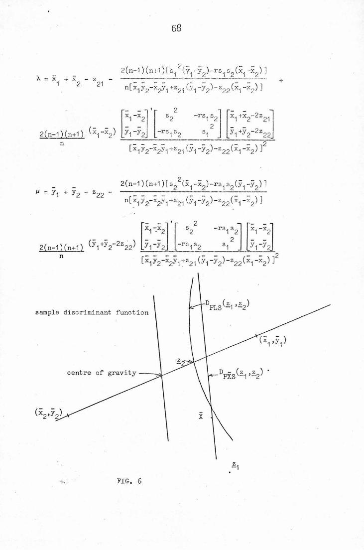
68

2(n-1)(n+1)[Sl"(y1 -y2)"rsiS2(*1 -x2)]X = x + - z - 3— ■' — 3———:—21 n[x1y2-x2y1+z21(y1-y2)-z22(x1-x2)]

r-— — "11r 2

X1 ~x2 s2 -rs1s2 X1+X2~2Z21

2(n-l)(n+l) (xi-x2) y1 -y22

-rs.Sg s1 /1+y2-2z22- - - - _ _ _ 2

[x1y2-x2y1 +z21 (y1-y2)-z22(x1~x2^ ^

sample discriminant function

2(n-1) (n+1) [ s22(5c1 -Xg)-rs, s2(y1 -y2) 1n[x1y2-x2y1+z21 (y1-y2)-z22(x1-*2)]

X1 -x2 "rS1S2-T'r. ^

x1-x2

Ly1 ~y2J

[x1y2-x2y1 +z21 (yi-y2)-z22(x^-x2) T

centre of gravity - (z , z ) *PXSV-1'-2y

*1

FIG. 6

We observe from the above diagram that when lies on—2

the line joining the sample means, the situation may arise whereby

D and D - differ in their sexing of the pair. Obviously, similari L o i X S

conflicting results will occur when m/n and neither of the pair lies

on the line joining the sample means. The only exception to this

general rule is when m=n and one of the pair lies at the centre of

gravity (since D and D - are then equivalent).r.Lo rXo

(2-11) AN EXAMPLE OF THE USE OF DOT_jLl)

The male and female of the fulmar are almost indistinguishable

in external appearance ; only by dissection can wre be certain about the

sex of a bird. However, there are slight differences in bill-length

and bill-depth between the male and female of the species. As there

is some overlap of these measurements and they are often available in

pairs, it looks as if we can apply to good effect. Note also

that since it is known that there are equal numbers of male and female

fulmars in the whole population, our assumption of equal prior probabilities

is valid.

The sample data used was from Figure 2 of Dunnet and

Anderson(l961). From the sample of 17 males and 17 females, the sample

discriminant function (D ) was calculated to beO

Bill depth = -0*7553Bill length + 46-94-75

or y = -0 *7553x + 46*94-75

Notice that this differs slightly from Dunnet and Anderson's discriminator

(y = -0 *5068x + 37*0958) since the data we used was only approximated

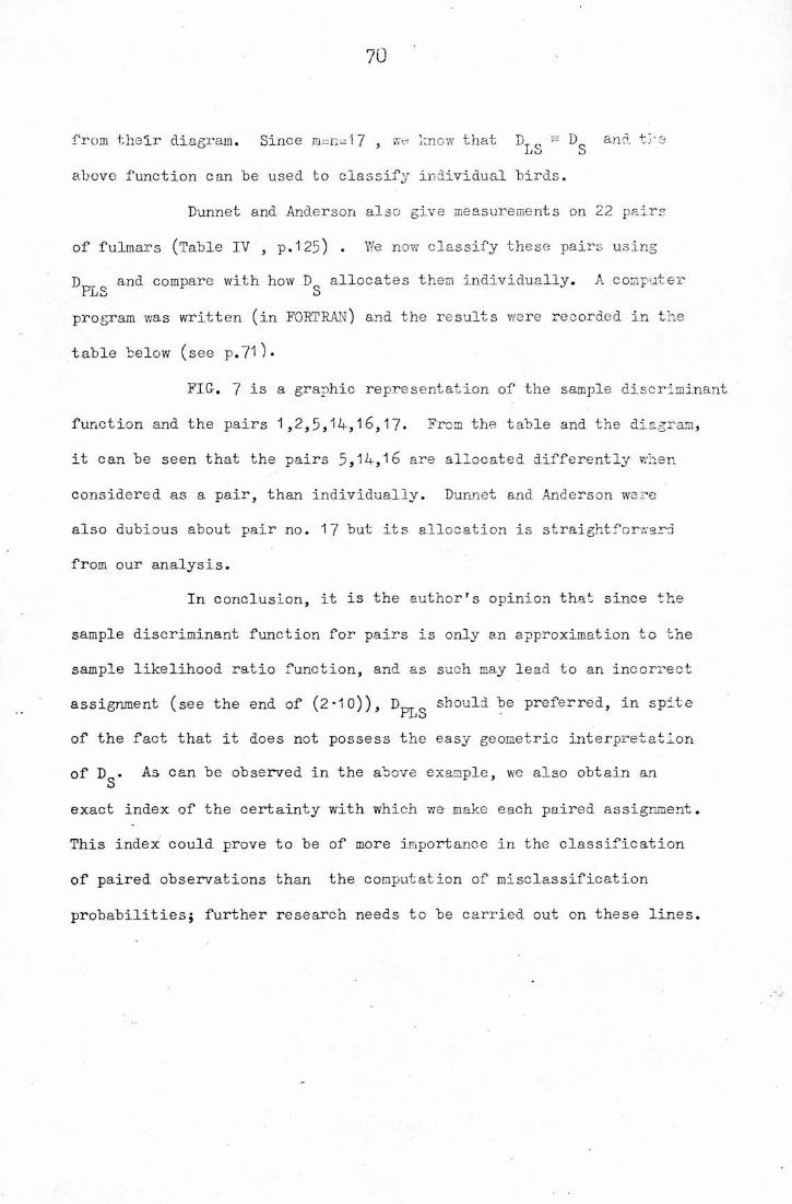
from their diagram. Since m=n-17 , we know that D = D and theLo d

above function can be used to classify individual birds.

Dunnet and Anderson also give measurements on 22 pairs

of fulmars (Table IV , p.125) • We now classify these pairs using

D _ and compare with how D allocates them individually. A computerPLS S

program was written (in FORTRAN) and the results were recorded in the

table below (see p.7l)-

FIG. 7 is a graphic representation of the sample discriminant

function and the pairs 1,2,5,14,16,17- From the table and the diagram,

it can be seen that the pairs 5,14,16 are allocated differently when

considered as a pair, than individually. Dunnet and Anderson were

also dubious about pair no. 17 but its allocation is straightforward

from our analysis.

In conclusion, it is the author's opinion that since the

sample discriminant function for pairs is only an approximation to the

sample likelihood ratio function, and as such may lead to an incorrect

assignment (see the end of (2-10)), D should be preferred, in spiteiLo

of the fact that it does not possess the easy geometric interpretation

of D • As can be observed in the above example, we also obtain anS

exact index of the certainty with which we make each paired assignment.

This index could prove to be of more importance in the classification

of paired observations than the computation of misclassification

probabilitiesj further research needs to be carried out on these lines.

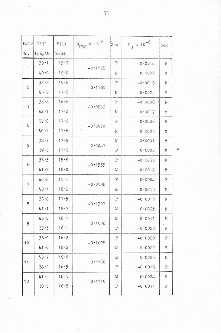
71

Pair Bill Bill x 1 0"6FLS

Sex D0 x 10 6O

Sex

No. Length Depth

39-1 15-7 F -0 *0014 F1 -0*1158

40 *6 19-0 M 0 *0022 M

38-2 15-8 F -0 *0019 F2 -0*1160

43*0 17-6 M 0 *0025 M

38*8 16*6 F -0*0008 ' F3 -0*0859

42 -1 17*2 M 0*0017 M

37-8 17-6 F -0*0006 F4 -0*0470

40 -1 17-6 M o *0003 M

38-7 17-9 M 0 *0001 M

5 0 *004739*0 17*5 F 0*0000 M

36-3 15*8 F -0*0030 F6 -0*1535

41 -2 18*0 M 0 *0018 M

40-8 15*7 F -0*0004 F

7 -0*058840-1 18*2 M o *0013 M

36-8 17*5 F -0*0013 F8 -0*1327

41 -1 18*7 M 0*0023 M

40-0 18*1 M 0 *0011 M

9 0*105837*3 16*1 F -0*0022 F

36-0 16*2 F -0 *0029 F10 -0*1628

41 *6 18*2 M 0 *0022 M

40-7 19*0 M 0*0023 M11 0*1160

38-2 16*5 F -0 *0013 F

41 -5 18*5 M 0 *0024 M12 0*1110

38-5 16*5 F 1 O o o —X F

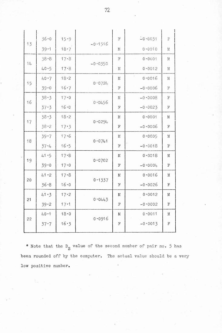
36-0 15-9 F -0-0031

l

F

13 -0-151639-1 18-7 M 0-0010 M

38-8 17-8 F 0-0001 M

14 -0-035040-5 17-8 M 0-0012 M

40-7 18*2 M 0-0016 M

15 0-072439-0 16-7 F -0-0006 F

38-3 17-0 M -0-0008 F

16 0-045637-3 16-0 F -0-0023 F

38-3 18-2 M 0-0001 M

17 0-029438-2 17-3 F -o-ooo6 F

39-7 17-6 M 0-0005 M

18 0-074137-4 16-5 F -0-0018 F

41 -5 17-8 M 0-0018 M

19 0-070239*0 17-0 F 1 o o o o *r F

41 -2 17*8 M 0-0016 M20 0-1337

36-8 16-0 F -0-0026 F

41 -3 17-2 M 0 -0012 M21 0 -0443

39*2 17-1 F -0-0002 F

40-1 18-0 M 0 -0011 M22 0-0916

37-7 16-3 F -0-0013 F

* Note that the DQ value of the second member of pair no. 5 has

been rounded off by the computer. The actual value should be a very

low positive number.

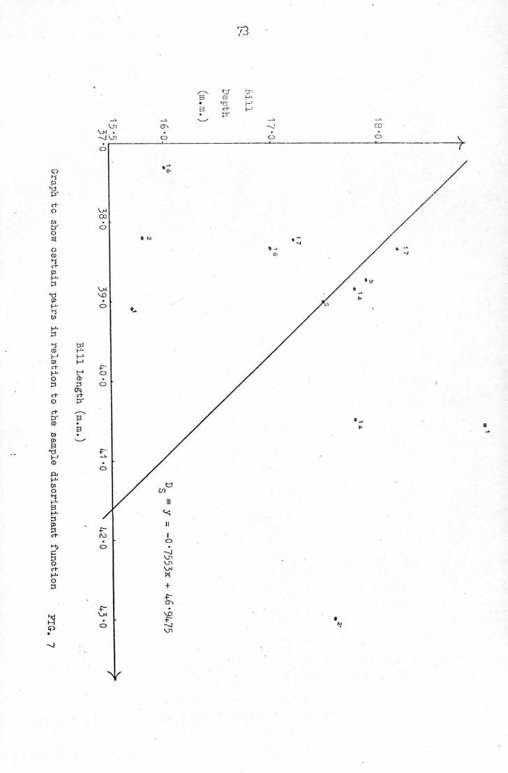
G-raphto

show

certainpairsin

relationto

the

sample

discriminantfunction

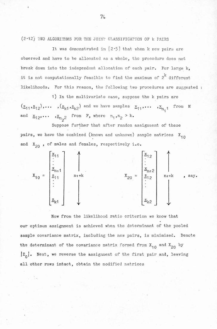
(2*12) TWO ALGORITHMS FOR THE JOINT CLASSIFICATION OF k PAIRS

It was demonstrated in [2-5] that when k new pairs are

observed and have to be allocated as a whole, the procedure does not

break down into the independent allocation of each pair. For large k,lr

it is not computationally feasible to find the maximum of 2^ different

likelihoods. For this reason, the following two procedures are suggested

1) In the multivariate case, suppose the k pairs are

(l-l-l >112) ' * * * '(-k1'-k2^ and WS have saraPles >2^ 1 from Mand X-] 2' * * ' ,x n from F, where n.,n„ > k.

-7^2^ 12Suppose further that after random assignment of these

pairs, we have the combined (known and unknown) sample matrices X^ ^

and X£q j of males and females, respectively i.e.

10

-1-1

-ml

-11

*k1

m +k20

-12

—n2 2

-12

■k2

n2+k say.

•V

Now from the likelihood ratio criterion we know that

our optimum assignment is achieved when the determinant of the pooled

sample covariance matrix, including the new pairs, is minimised. Denote

the determinant of the covariance matrix formed from X._ and X„„ by10 20

|2q[. Next, we reverse the assignment of the first pair and, leavingall other rows intact, obtain the modified matrices

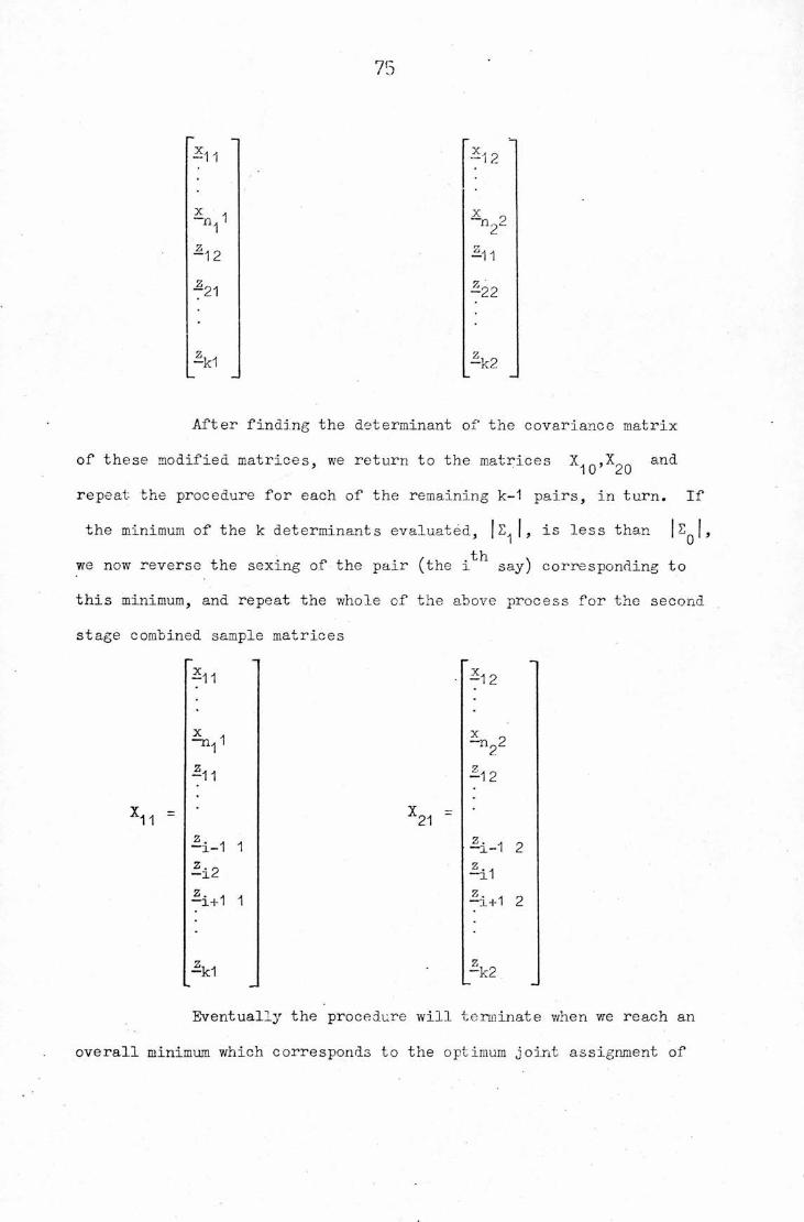
75

-11

2£ 1V-12

-21

*k1

-12

x ,

2C

-11

-22

—k2

After finding the determinant of the covariance matrix

of these modified matrices, we return to the matrices X,„,X„„ and' 10 20

repeat, the procedure for each of the remaining k-1 pairs, in turn. If

the minimum of the k determinants evaluated, j [, is less than |I,we now reverse the sexing of the pair (the i ^ say) corresponding to

this minimum, and repeat the whole of the above process for the second

stage combined sample matrices

11

x,.—11

-11

—i-1 1

—i2

-i+1 1

—k1

X21

-12

21n22-12

-i-1 2

^11

-i+1 2

—k2

Eventually the procedure will terminate when we reach an

overall minimum which corresponds to the optimum joint assignment of

76

the k pairs. This optimum car he checked "by starting from different

random assignments.

A modification of this algorithm is for the initial

assignment not to be random but that of the pairs considered separately.

Then the optimum should be reached in fewer iterations e.f. Beale('J 971) ,

who observes that, with reference to cluster analysis, "in general, a

good starting solution leads to a good final solution".

2) Alternatively, we make an initial random assignment

of the first k-1 pairs to get the combined sample matrices ,i ,k

and X2,k

where

1,k

-11

xi

-n11*11

-k-1 1

n +k-11

X2,k

-n22-12

-k-1 2

n2+k-1

we use D

Then, treating X^ and X^ , as known sample matrices,I y ilC ^ j K

to classify the kth pair. Tie next omit the (k-1 ) ^PLS

pair and classify it using DCT formed from the matrices X andX J_J O I y K— I

X2,k-1 *'here

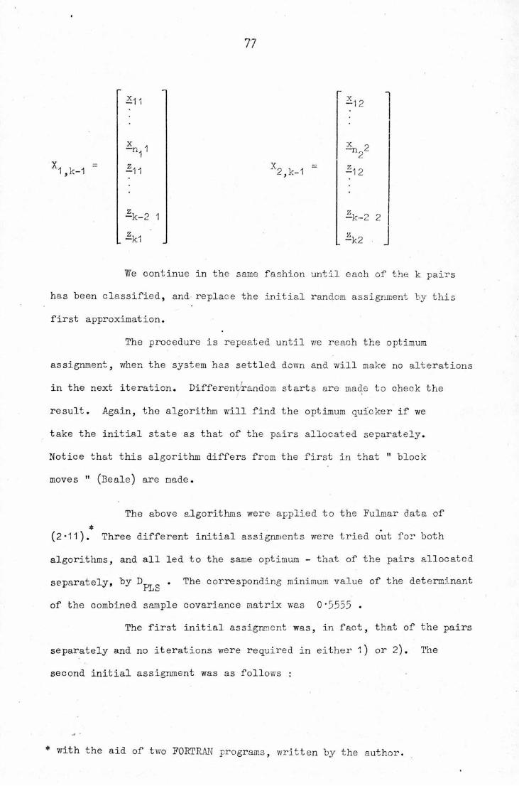
77

x1 ,k-1

-11

x -i

~n1^11

—k-2 1

*k1

X2,k-1

x12

22

-12

—k~2 2

-k2

We continue in the same fashion until each of the k pairs

has been classified, and- replace the initial random assignment by this

first approximation.

The procedure is repeated until we reach the optimum

assignment, when the system has settled down and will make no alterations

in the next iteration. Differentrandom starts are made to check the

result. Again, the algorithm will find the optimum quicker if we

take the initial state as that of the pairs allocated separately.

Notice that this algorithm differs from the first in that " block

moves " (Beale) are made.

The above algorithms were applied to the Fulmar data of*

(2*11). Three different initial assignments were tried out for both

algorithms, and all led to the same optimum - that of the pairs allocated

separately, by D . The corresponding minimum value of the determinantHLS

of the combined sample covariance matrix was 0*5555 .

The first initial assignment was, in fact, that of the pairs

separately and no iterations were required in either l) or 2). The

second initial assignment was as follows :

* with the aid of two FORTRAN programs, written by the author.

78

Pairs 1,5,21 the same way round as allocated by D Q in

the table of (2-11) ; pairs 2,3,4,6,... ,20,22 the opposite to that

of the table in (2*11).

For algorithm 1) , the values of the determinant, and

the number of the actual pair altered, at each iteration, are given

in the table on page 79* Notice that pair no. 1 is the first pair

to be altered but reverts to its initial assignment at the 15 ^ iteration.

Algorithm 2) only required two iterations but, of course, block moves

were made. The D values of the pairs, based on samples of sizePLS

n^+k-1 and n +k-1 , for each iteration are also given in the tableon page 79. Again pair no. 1 and also pair no. 5 this time, are altered

at the first iteration, but then revert to their initial assignment.

Note too, the suspicion with which pair no. 17 is treated before it is

finally allocated, thus confirming Dunnet and Anderson's doubts. Finally?

it is worth making a comparison between the tables on p. 7-j and p. 79

of the order of the pairs, in terms of likelihood (D value). When1JJS

classified separately, the order (from the largest likelihood downwards)

of the pairs is

10 613 20 811 2 1 12 9 22 3181519 7 4 16 21 14 17 5

Similarly, when considered as a whole, the order is

10 6 13 2 20 1 11 12 9 8 22 15 18 3 19 7 16 21 4 17 14 5

Clearly, since the two orders are not equivalent, when we

take all the 22 pairs into account in our discriminant procedure, we

become more certain that we have made a correct decision with some

pairs e.g. no. 2 , but less confident about others e.g. no. 4 .

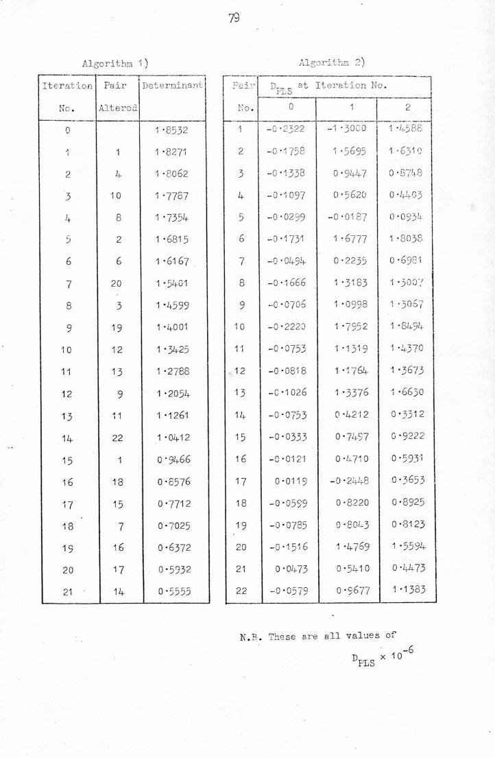
79

Algorithm 1)

Iteration

No.

i

Pair

Altered

Determinant

o 1 -8532

1 1 1-8271

2 4 1-8062

3 10 1-7787

4 8 1 -7354

5 2 1 -6815

6 6 1 -61 67

7 20 1-5401

8 3 1 -4599

9 19 1-4001

1 0 12 1 -3425

11 13 1 -2788

12 9 1-2054

13 11 1 -1261

14 22 1 -0412

15 1 0-9466

16 18 0-6576

17 15 0-7712

18 7 0-7025

15 16 0-6372

20 17 0-5932

21 ' 14 0 -5555

Algorithm 2)

Dt-t r- a"t Iteration NFLSa.

0 1 2

-0 -2322 -1-3000 1 -4588

-0-1758 1 -5695 1 -6310

-0-1338 0-9447 0-8748

-0-1097 0-5620 0-4403

-0-0299 -0-0187 0-0934

-0-1731 1-6777 1-8038

-0-0494 0-2235 0-6981

-0•1066 1 -3183 1-3007

-0-0706 1 -0998 1 -3067

-0-2220 1 *7952 1 -8494

-0-0753 1 -1319 1 -4370

-0-0818 1 -1764 1-3673

-0-1026 1 -3376 1 -6630

-0-0753 0-4212 0-3312

-0-0333 0-7457 0 -9222

-0-0121 0 -4710 0-5931

0-0119 -0-2448 0-3653

-0-0599 0-8220 0-8925

-0-0785 0-8043 0-8123

-0-1516 1 -4769 1 -5594

0-0473 0-5410 0-4473

-0-0579 0-5677 1 -1383

. These are all values of

Pair

7\T r~\

2

3

4

5

b

7

8

9

1 0

11

12

13

14

15

16

17

18

19

20

21

22

N.B

80

The third initial assignment was the opposite of the second i.e., only

the pairs 1,5,21 differed from the optimum ; this was achieved after

three iterations of Algorithm 1) and one of Algorithm 2).

We conclude (2-12) with a. warning about the use of the

two algorithms. When the original known samples were reduced to a

randomly chosen 5 from each sex, the algorithms produced conflicting

results for the above three initial assignments. From the first and

third, the usual optimum assignment was attained ; however, from the

second initial assignment, both algorithms led to the exact opposite

of the usual optimum i.e-. ail the males of the optimum were classified

as F, a.nd all the females as M.

Thus, when the original sample sizes n^,n^ < k , thenumber of pairs, the above results indicate that we either accomplish

the true optimum or an outcome close to its opposite. To counter this

effect, it is suggested that Algorithm 1) should be employed with the

following modification :

When the system has reached a local optimum, this

allocation is reversed. If the determinant of the covariance matrix

of this reversal is lower than the determinant of the covariance matrix

of the local optimum, the algorithm should continue with this new

initial assignment until it reaches the true optimum. If the determinant

corresponding to the local optimum is lower than that of its opposite,

it is in fact the true optimum. Algorithm 2) may now be used to

calculate D„ values, whereby we can tell which pairs are morePLS

likely to have been correctly classified.

(2*13) CONCLUSION

By means of the likelihood ratio criterion, we have

developed and analysed a theoretically exact procedure for the assignment

of paired observations. The usefulness of this procedure is evident

from the results, that we obtained, of its application to some Fulmar

data. When the new pairs have to be assigned a.s a whole, the two

algorithms (with modifications for small sample sizes) also seemed

to work well with respect to the same data. Notice that throughout

the thesis, the theory is always simplified if we consider the sample

sizes, of the original known data, to be equal ; obviously, this

condition will always be satisfied if the original samples are, in

fact, pairs.

Although further research needs to be conducted, such as

into the best method for estimating paired misclassification probabilities

the thesis serves as an introduction to this particular branch of

discriminant analysis.

The author wishes to thank Prof. R.M. Cormack for suggesting

the problem and for many helpful discussions during the course of this

research. The work was supported by a St. .Andrews University research

grant.

82

REFERENCES

ANDERSON, T.W. (1958). An introduction to multivariate statistical

analysis. John Wiley, New York.

BARNARD, M.M. (1935). The secular variation of skull characters in

4 series of Egyptian skulls. Ann. Eugenics, Vol. 6, p. 352.

BARTLETT, M.S. (1951)• An inverse matrix adjustment arising in

discriminant analysis. Ann. Math. Stat., 22, p. 107.

BEA1E, E.M.L. (1971)- Erom the discussion on Prof. Cormack's paper :

A review of classification. J.R.Stat. Soc. (A), 134, p. 321.

COCHRAN, W.G. and BLISS, C.I. (1948). Discriminant functions with

covariance. Ann. Math. Stat., 19, p. 151.

CRAMER, E.M. (19^7)• The equivalence cf two methods of computing

discriminant function coefficients. Biometrics, 23, p. 153-

DAS GUPTA, S. (1968). Some aspects of discriminant function

coefficients. Sankha A, 30, p. 387*

DUKNET, G.M. and ANDERSON, A. (1961). A method for sexing living

fulmars in the hand. Bird Study, Vol. 8, No. 3, P« 119.

FISHER, R.A. (1936). The use of multiple measurements in taxonomic

protlems. Ann. Eugenics, 7, p. 179.

FISHER, R.A. (1938). The statistical utilisation of multiple

measurements. Ann. Eugenics, 8, p. 376.

83

FISHER, R.A. (1940). The precision of discriminant functions. Arm.

Eugenics, 10, p. 422.

HEA1Y, M.J.R. (1965). Computing a discriminant function from within

sample dispersions. Biometrics, 21, p. 1011.

HILLS, M. (1966). Allocation rules and their error rates. J.R.Stat.

Soc. (B), 23, p. 1 .

HOEL, P.O. and PETERSON, R.P. (1949)- A solution to the problem of

optimum classification. Ann. Math. Stat., 20, p. 433•

HOTELLING, H. (1931). Generalisation of Student's Ratio. Ann. Math.

Stat., 2, p. 360.

HOTELLING, H. (1936). Relations between 2 sets of variates. Biometrika,

28, p. 321.

JOHNSON, N.L. and K0T2, S. (1970). Continuous univariate distributions II.

Houghton Mifflin, Boston.

JONES, A.C. (1912). An introduction to algebraical geometry, Oxford.

KSHIRSAGAR, A.M. (1972). Multivariate Analysis. Marcel Dekker, Inc.,

New York.

LACHENBRUCH, P.A. (1965). Estimation of error rates in discriminant

analysis. Ph.D. Dissertation, University of California, Los Angeles.

LACHENBRUCH, P.A. and MICKEY, M.R. (1968). Estimation of error rates

in discriminant analysis. Technometrics, 10, p. 1.

MAHALANOBIS, P.C. (192/). Analysis of race mixture in Bengal. J cum.

Asiat. Soc. Bengal, 23, p. 301.

MAHALANOBIS, P.C. (1 930). On test measures of group divergence. Journ.

Asiat. See. Bengal, 26, p, 541.

MARTIN, E.S. (1936). A study of an Egyptian series of mandibles with

special reference to mathematical methods of sexing. Biometrika,

28, p. 149.

MORRISON, D.F. (1967). Multivariate statistical methods. McGraw-Hill.

NATIONAL BUREAU OF STANDARDS (1959)• Tables of the bivariate normal

distribution function and related functions. Applied Maths.

Series 50, U.S. Government Printing Office, Washington D.G..

0KAM0T0, M. (1963). An asymptotic expansion for the distribution of

the linear discriminant function. Ann. Math. Stat., 34, p. 1286.

PEARSON, K. (1926). On the coefficient of racial likeness. Biometrika,

18, p. 105.

PENROSE, L.S. (1947). Some notes on discrimination. Ann. Eugen., 13,

p. 228.

RAO, C.R. (1946). Tests with discriminant functions in multivariate

analysis. Sankhya, 7, p. 407.

RAO, C.R. (1949). On some problems arising out of discrimination with

multiple characters. 'Sankhya, 9, P« 343.

85

RAO, C.R*. (1965). Linear statistical inference. John Wiley, Lew York,

SITGREAVES, R. (1952). On the distribution of two random matrices used

in classification procedures. Ann. Math. Stat., 23, p. 263,

WALE, A. (1°44). On a statistical problem arising in the classification

of an individual into one of two groups. Ann. Math, Stat., It,

p. 145.

WELCH, B.L. (1939), A note on discriminant functions. Biometrika, 31,

p. 218.

University of St Andrews - St Andrews Research Repository

Documents