Unit 3

UNIT III

Scan conversion and Output Primitives

1

Line drawing algorithm

• Computer screen is divided into rows and columns.

• The intersection area is known as pixel.• Process of determining which combination

of pixels provide the best approximation of a desired line is known as Rasterization

• Rasterization is combined with rendering of the picture in scan line order, then it is known as scan conversion.

2

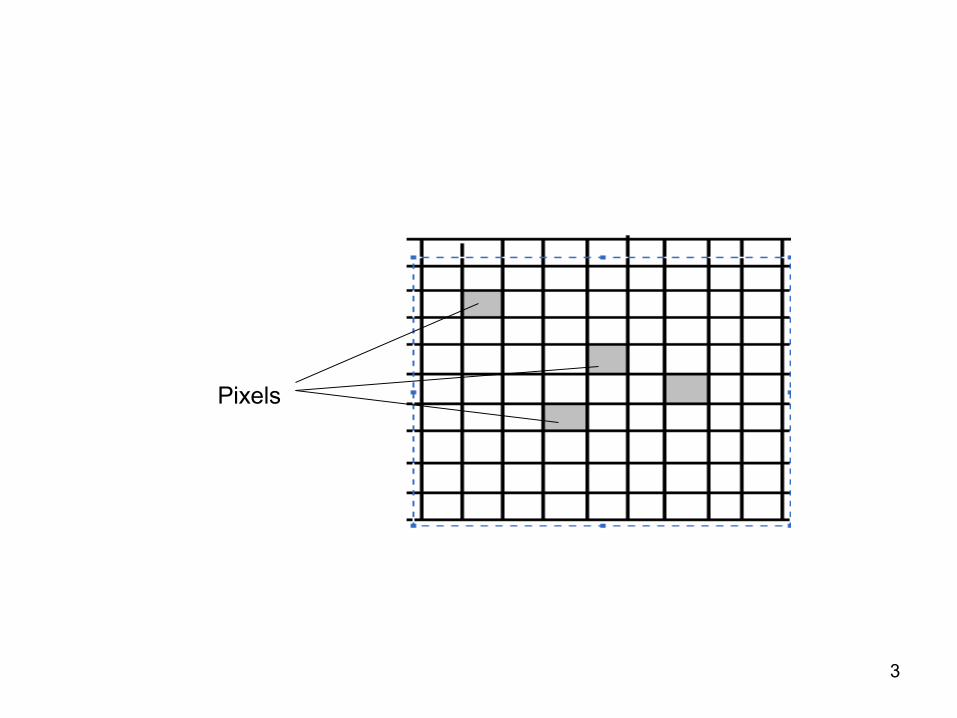
Pixels

3

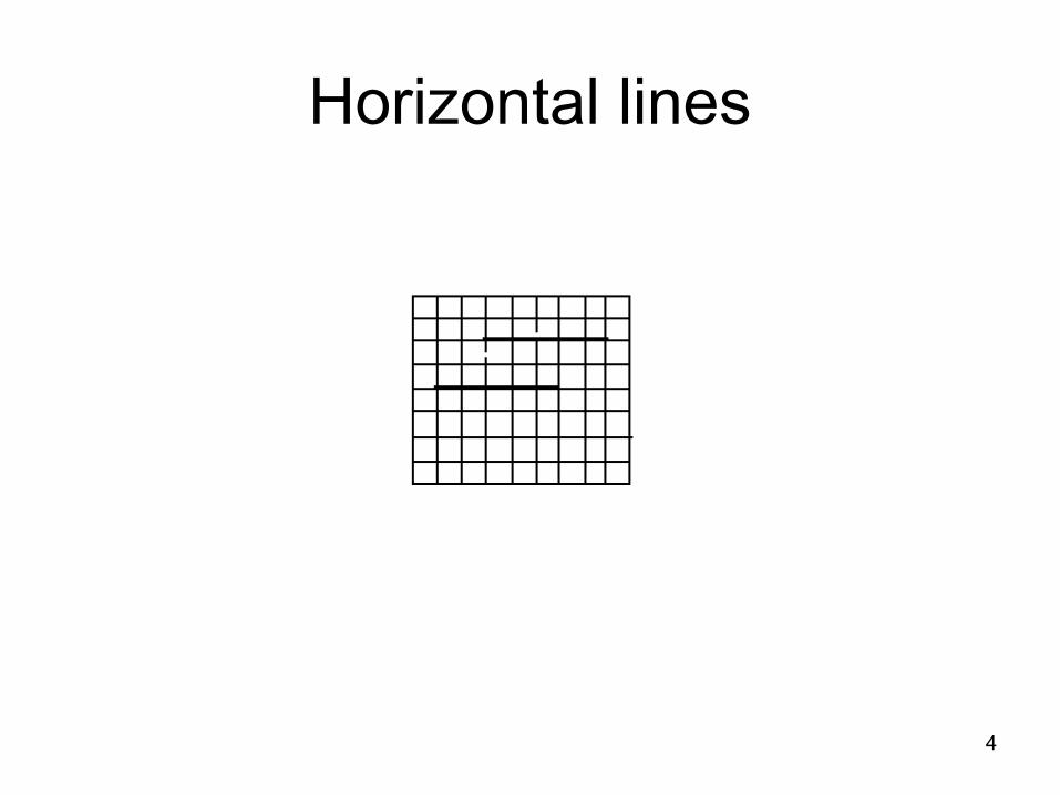
Horizontal lines

4

General requirement for requirement of a line

• Line must appear to be straight

• Lines should start and end accurately

• Lines should have constant brightness along their length.

• Lines should be drawn rapidly

5

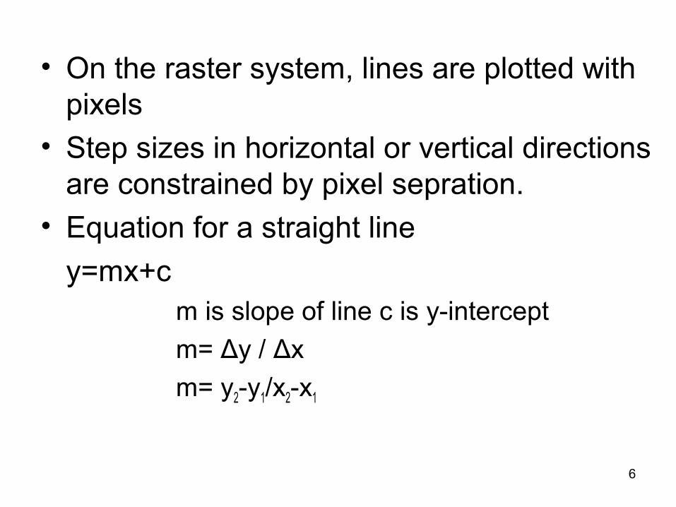
• On the raster system, lines are plotted with pixels

• Step sizes in horizontal or vertical directions are constrained by pixel sepration.

• Equation for a straight line

y=mx+cm is slope of line c is y-intercept

m= Δy / Δx

m= y2-y1/x2-x1

6

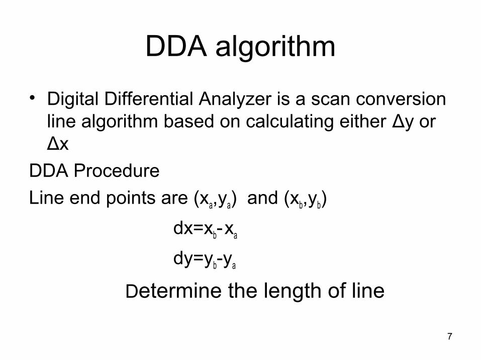
DDA algorithm

• Digital Differential Analyzer is a scan conversion line algorithm based on calculating either Δy or Δx

DDA Procedure

Line end points are (xa,ya) and (xb,yb)

dx=xb- xa

dy=yb-ya

Determine the length of line

7

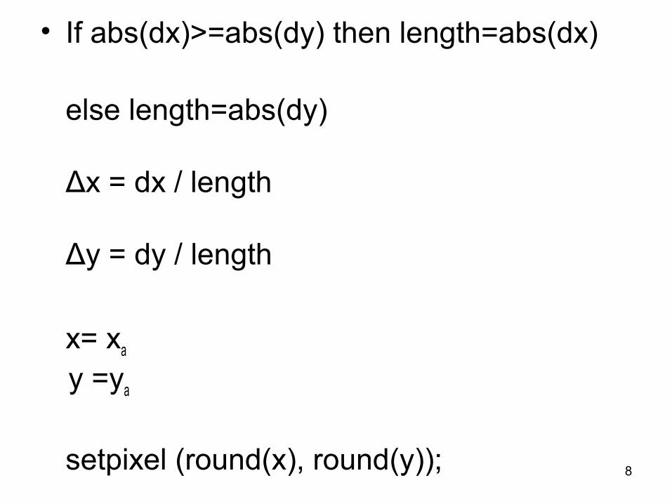
• If abs(dx)>=abs(dy) then length=abs(dx)

else length=abs(dy)

Δx = dx / length

Δy = dy / length

x= xa

y =ya

setpixel (round(x), round(y)); 8

9

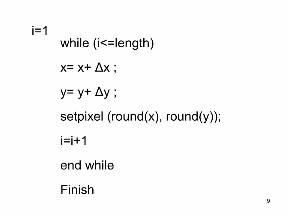
i=1while (i<=length)

x= x+ Δx ;

y= y+ Δy ;

setpixel (round(x), round(y));

i=i+1

end while

Finish

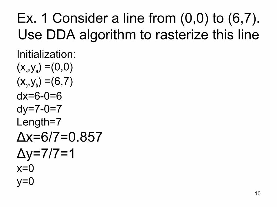
Ex. 1 Consider a line from (0,0) to (6,7). Use DDA algorithm to rasterize this lineInitialization:(xa,ya) =(0,0)(xb,yb) =(6,7)dx=6-0=6dy=7-0=7Length=7

Δx=6/7=0.857Δy=7/7=1x=0y=0

10

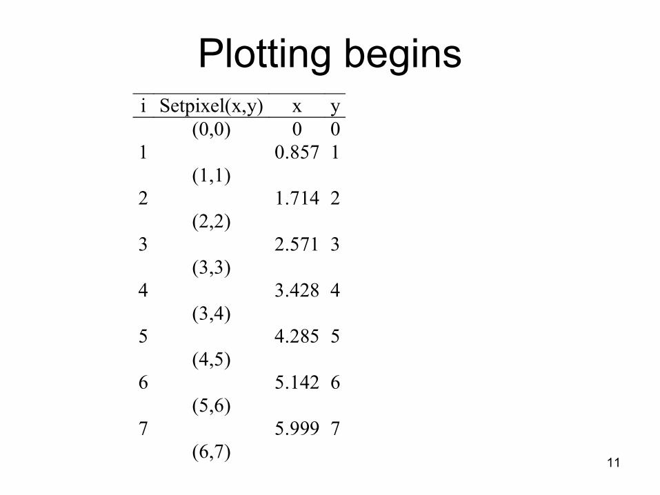
Plotting beginsi Setpixel(x,y) x y (0,0) 0 0

1 0.857 1 (1,1)

2 1.714 2 (2,2)

3 2.571 3 (3,3)

4 3.428 4 (3,4)

5 4.285 5 (4,5)

6 5.142 6 (5,6)

7 5.999 7 (6,7)

11

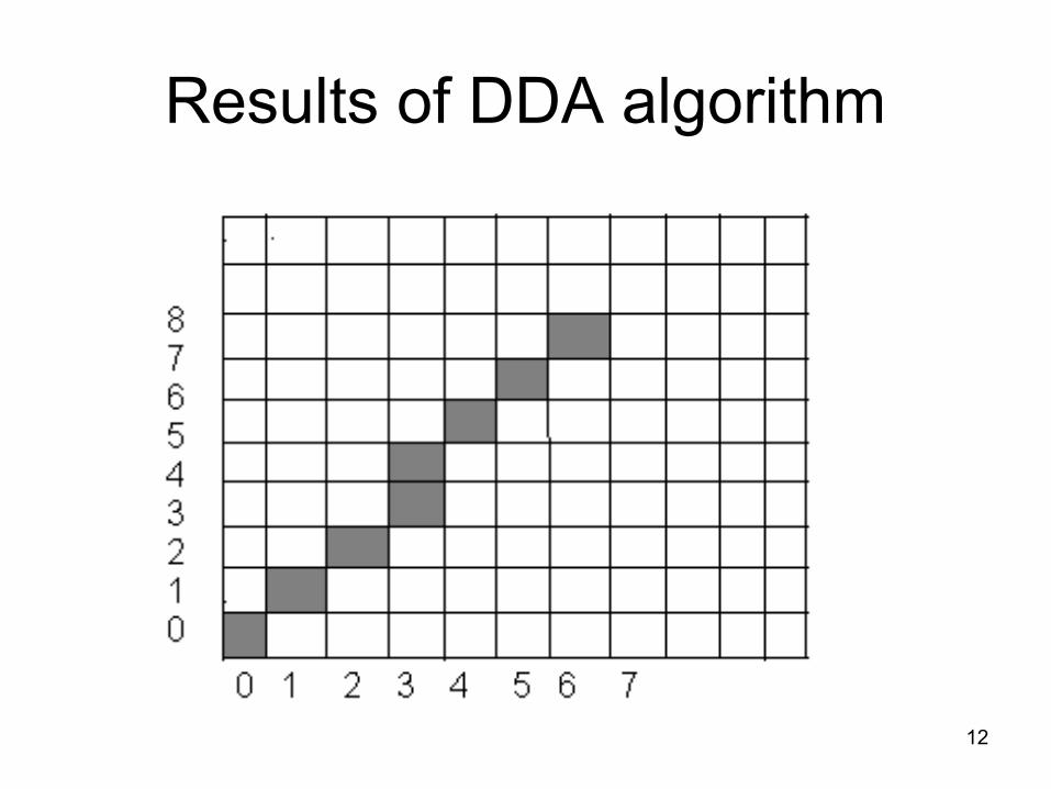
Results of DDA algorithm

12

Drawbacks

• Although fast, accumulation of round of error may drift the long line segments

• Rounding off is time consuming

13

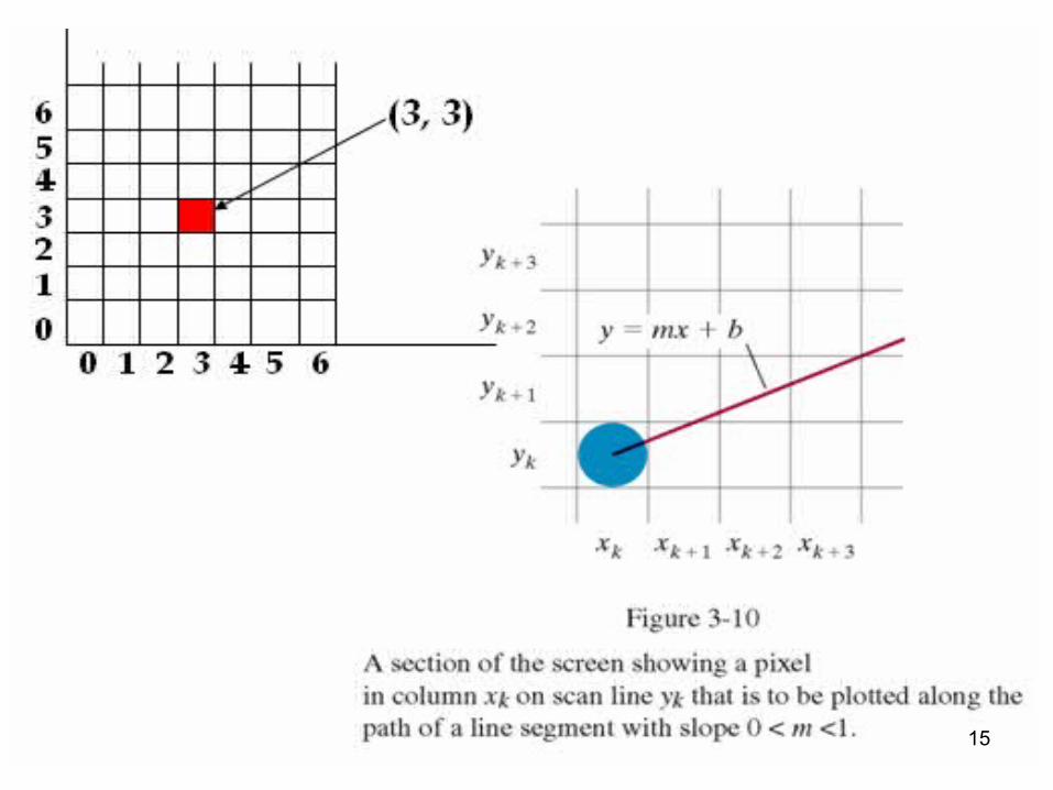
Bresenham’s line drawing Algorithm

• It determines which points in an n-dimensional raster should be plotted to form approximate straight line between two points.

• It chooses the integer y corresponding to the pixel center that is closest to the ideal (fractional) y for the same x; on successive columns y can remain the same or increase by 1.

• Depends upon the slope of the line.

14

15

16

17

18

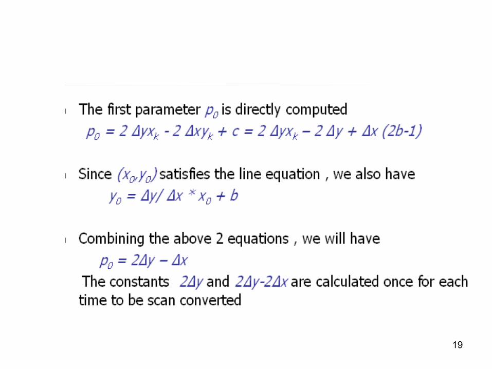
19

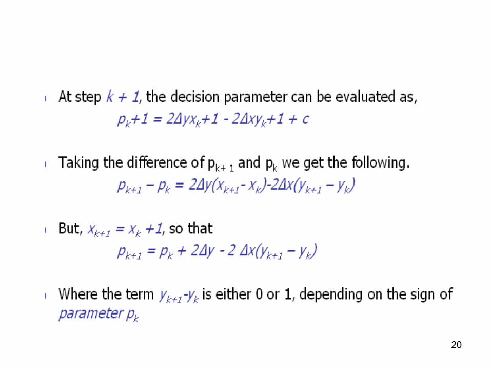
20

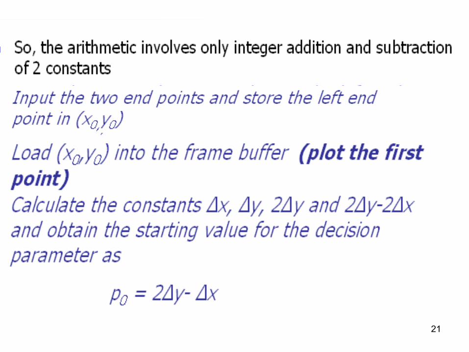
21

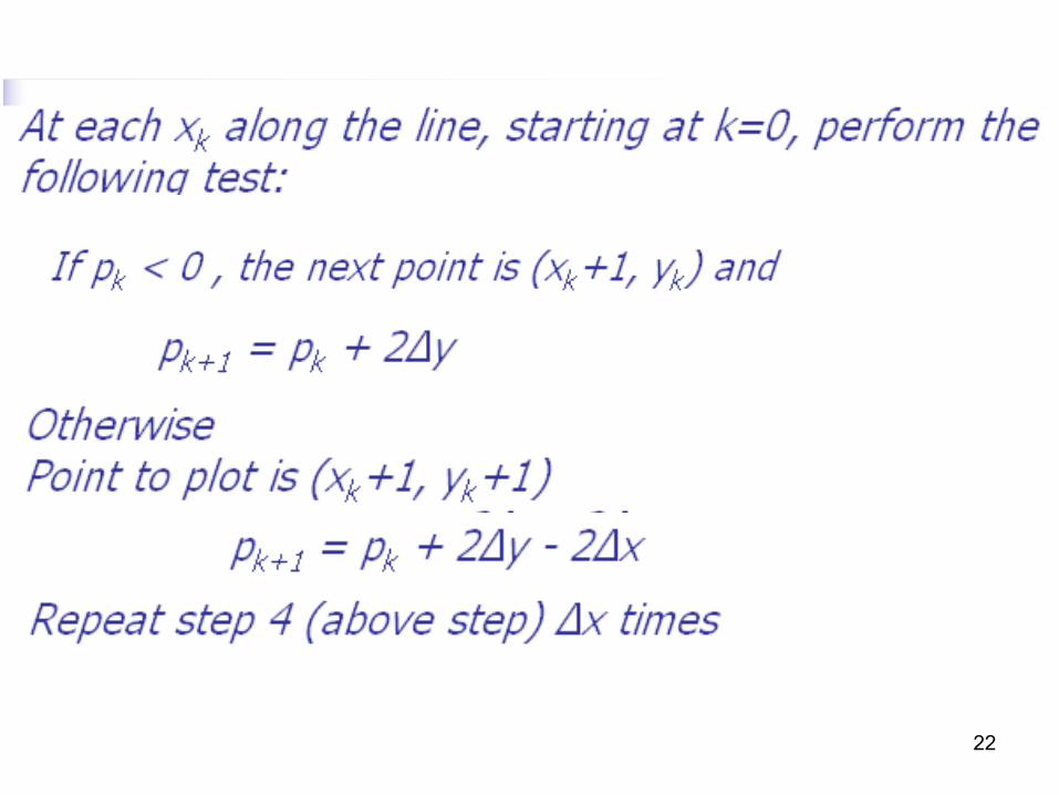
22

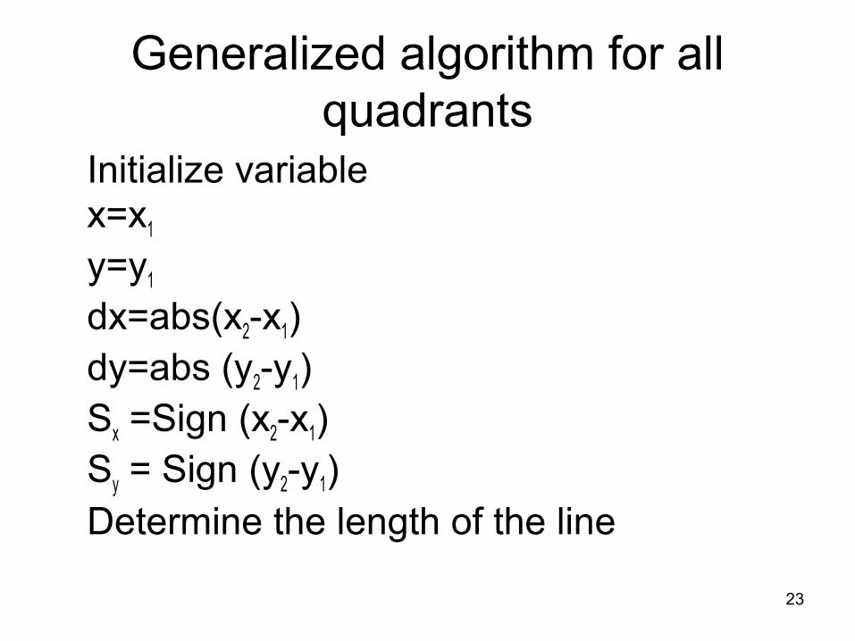
Generalized algorithm for all quadrants

Initialize variablex=x1

y=y1

dx=abs(x2-x1)dy=abs (y2-y1)Sx =Sign (x2-x1)Sy = Sign (y2-y1)Determine the length of the line

23

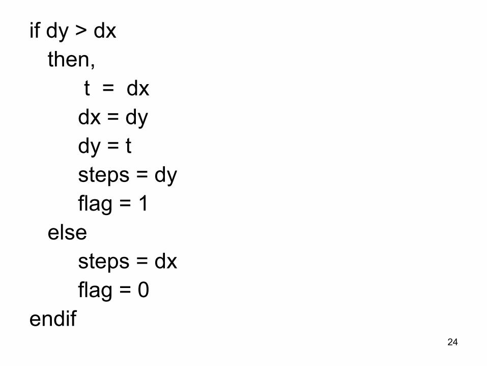
if dy > dxthen,

t = dxdx = dydy = tsteps = dyflag = 1

elsesteps = dxflag = 0

endif24

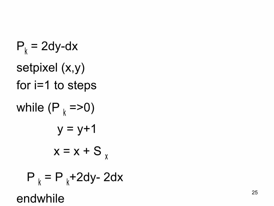
Pk = 2dy-dx

setpixel (x,y)

for i=1 to steps

while (P k =>0)

y = y+1

x = x + S x

P k = P k+2dy- 2dx

endwhile25

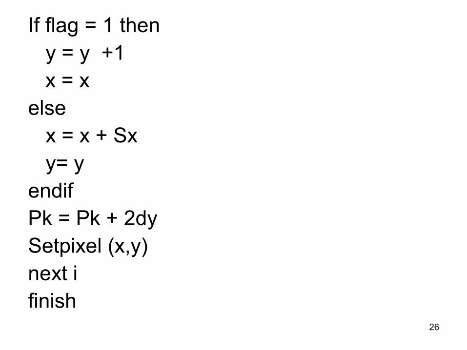
If flag = 1 theny = y +1

x = xelse

x = x + Sxy= y

endifPk = Pk + 2dySetpixel (x,y)next ifinish

26

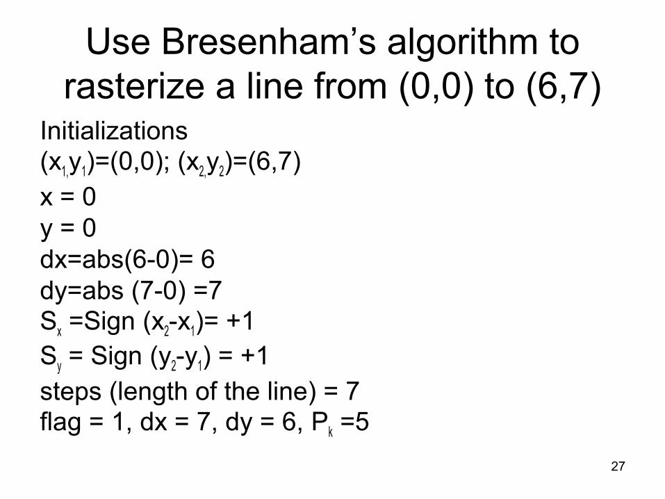
Use Bresenham’s algorithm to rasterize a line from (0,0) to (6,7)

Initializations(x1,y1)=(0,0); (x2,y2)=(6,7)x = 0y = 0dx=abs(6-0)= 6dy=abs (7-0) =7Sx =Sign (x2-x1)= +1Sy = Sign (y2-y1) = +1steps (length of the line) = 7flag = 1, dx = 7, dy = 6, Pk =5

27

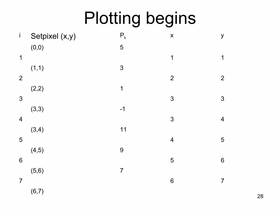
Plotting beginsi Setpixel (x,y) Pk x y

(0,0) 5

1 1 1

(1,1) 3

2 2 2

(2,2) 1

3 3 3

(3,3) -1

4 3 4

(3,4) 11

5 4 5

(4,5) 9

6 5 6

(5,6) 7

7 6 7

(6,7)28

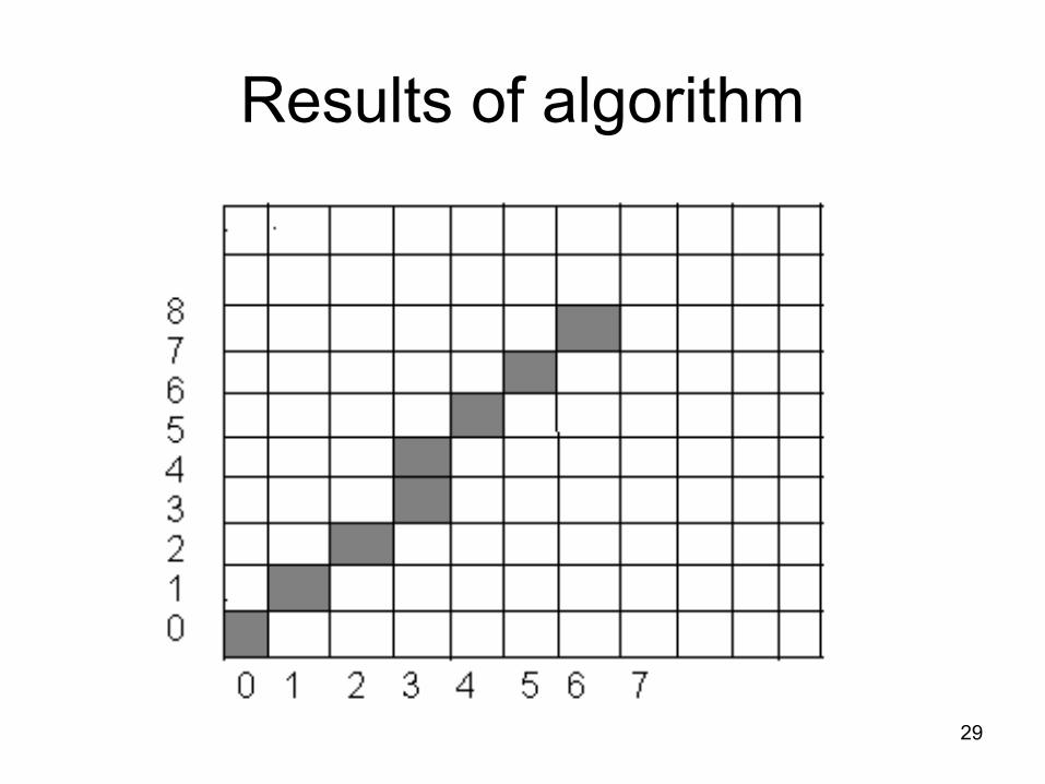
Results of algorithm

29

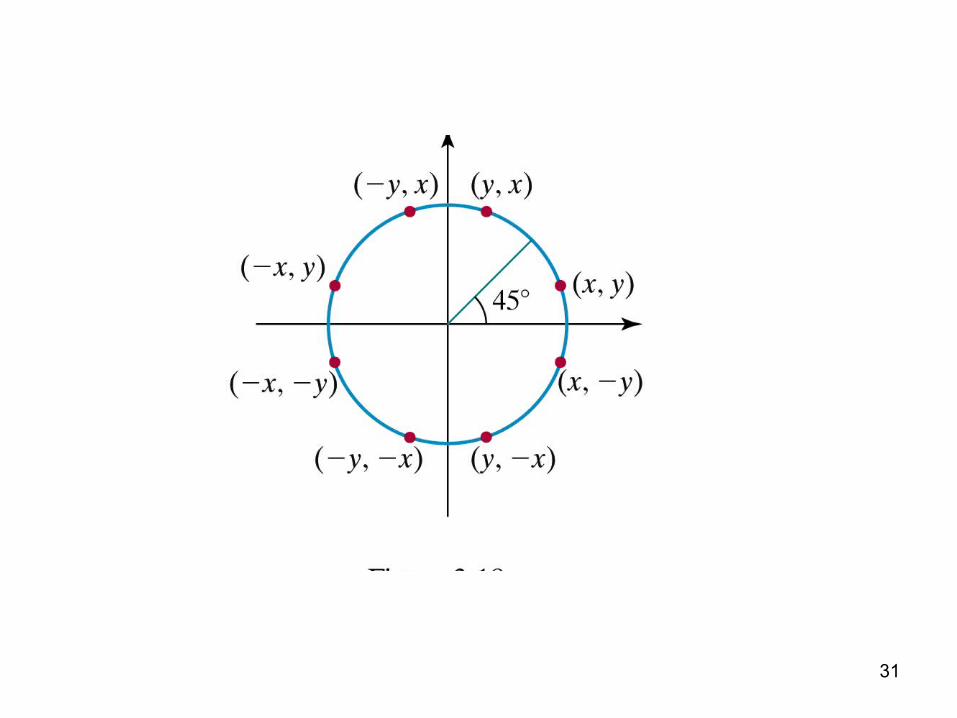
Bresenhem Circle drawing Algorithm

• Algorithm for 1st octant only

30

31

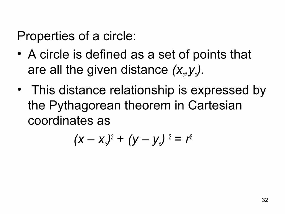
Properties of a circle:

• A circle is defined as a set of points that are all the given distance (xc,yc).

• This distance relationship is expressed by the Pythagorean theorem in Cartesian coordinates as

(x – xc)2 + (y – yc) 2 = r2

32

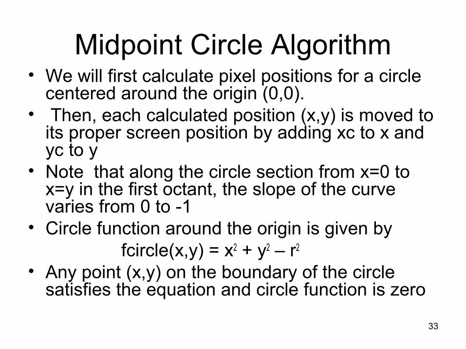
Midpoint Circle Algorithm• We will first calculate pixel positions for a circle

centered around the origin (0,0).• Then, each calculated position (x,y) is moved to

its proper screen position by adding xc to x and yc to y

• Note that along the circle section from x=0 to x=y in the first octant, the slope of the curve varies from 0 to -1

• Circle function around the origin is given byfcircle(x,y) = x2 + y2 – r2

• Any point (x,y) on the boundary of the circle satisfies the equation and circle function is zero

33

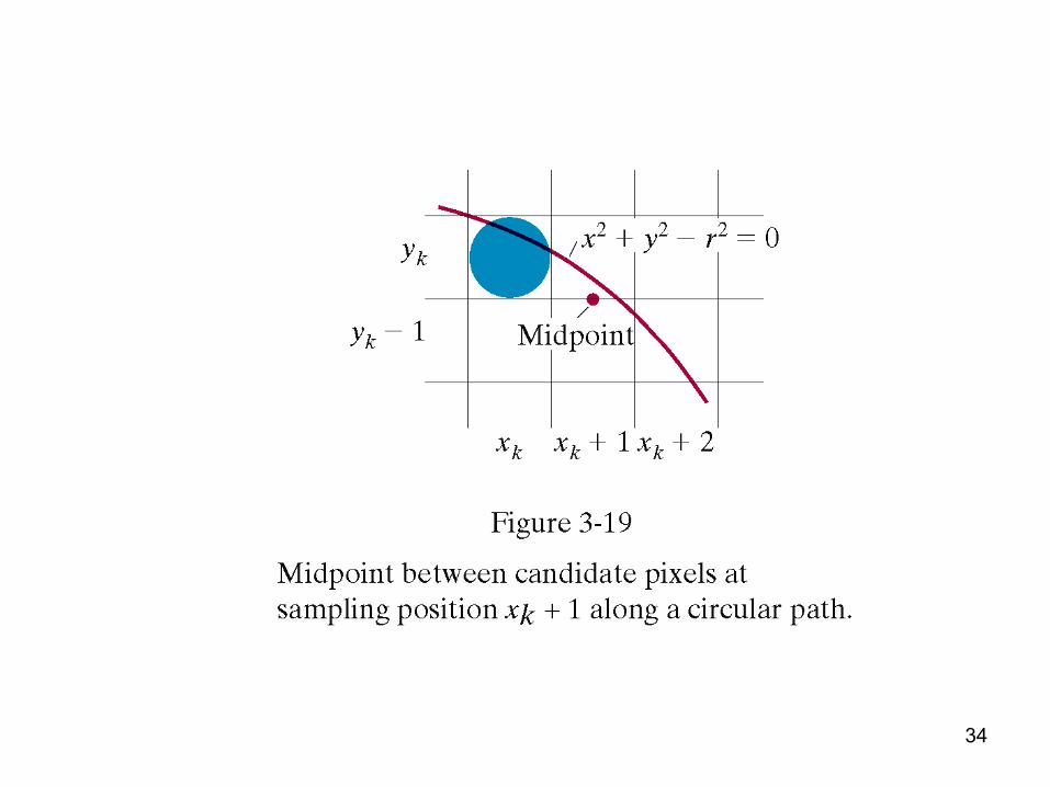
34

• For a point in the interior of the circle, the circle function is negative and for a point outside the circle, the function is positive

• Thus,– fcircle(x,y) < 0 if (x,y) is inside the circle

boundary– fcircle(x,y) = 0 if (x,y) is on the circle boundary– fcircle(x,y) > 0 if (x,y) is outside the circle

boundary

35

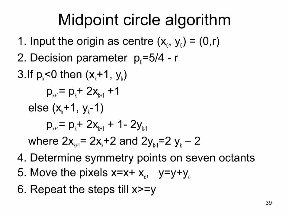
Midpoint circle algorithm1. Input the origin as centre (x0, y0) = (0,r)

2. Decision parameter p0=5/4 - r

3.If pk<0 then (xk+1, yk)

pk+1= pk+ 2xk+1 +1

else (xk+1, yk-1)

pk+1= pk+ 2xk+1 + 1- 2yk-1

where 2xk+1= 2xk+2 and 2yk-1=2 yk – 2

4. Determine symmetry points on seven octants5. Move the pixels x=x+ xc, y=y+yc

6. Repeat the steps till x>=y39

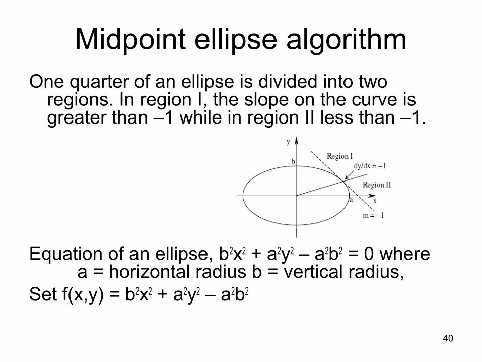
Midpoint ellipse algorithmOne quarter of an ellipse is divided into two

regions. In region I, the slope on the curve is greater than –1 while in region II less than –1.

Equation of an ellipse, b2x2 + a2y2 – a2b2 = 0 where a = horizontal radius b = vertical radius,

Set f(x,y) = b2x2 + a2y2 – a2b2

40

First point in ellipse centered on origin is (x0,y0)= (0,b)

Initial value of decision parameter

P0= f(1, b-1/2)

41

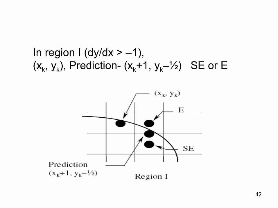
In region I (dy/dx > –1),(xk, yk), Prediction- (xk+1, yk–½) SE or E

42

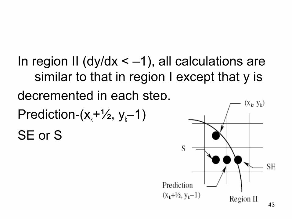
In region II (dy/dx < –1), all calculations are similar to that in region I except that y is

decremented in each step.

Prediction-(xk+½, yk–1)

SE or S

43

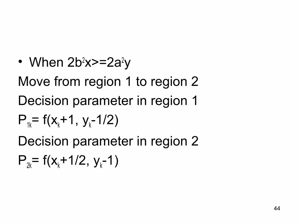
• When 2b2x>=2a2y

Move from region 1 to region 2

Decision parameter in region 1

P1k= f(xk+1, yk-1/2)

Decision parameter in region 2

P2k= f(xk+1/2, yk-1)

44

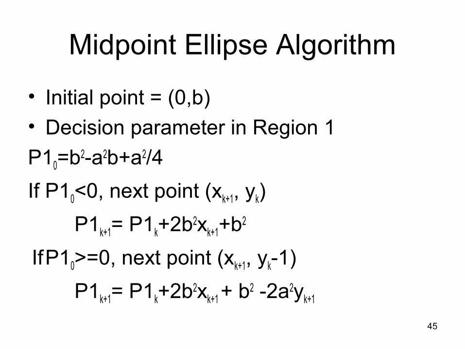
Midpoint Ellipse Algorithm

• Initial point = (0,b)

• Decision parameter in Region 1

P10=b2-a2b+a2/4

If P10<0, next point (xk+1, yk)

P1k+1= P1k+2b2xk+1+b2

If P10>=0, next point (xk+1, yk-1)

P1k+1= P1k+2b2xk+1 + b2 -2a2yk+1

45

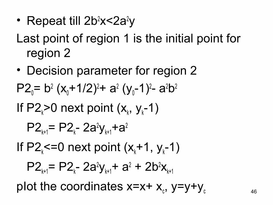
• Repeat till 2b2x<2a2y

Last point of region 1 is the initial point for region 2

• Decision parameter for region 2

P20= b2 (x0+1/2)2+ a2 (y0-1)2- a2b2

If P2k>0 next point (xk, yk-1)

P2k+1= P2k- 2a2yk+1+a2

If P2k<=0 next point (xk+1, yk-1)

P2k+1= P2k- 2a2yk+1+ a2 + 2b2xk+1

pIot the coordinates x=x+ xc, y=y+yc 46

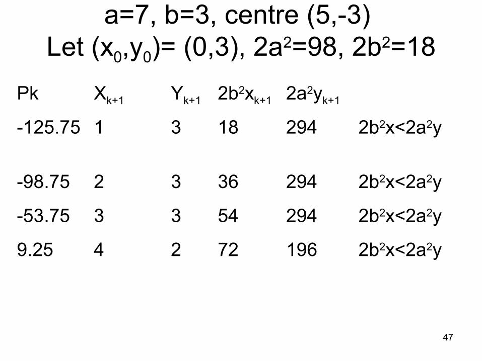
a=7, b=3, centre (5,-3) Let (x0,y0)= (0,3), 2a2=98, 2b2=18

Pk Xk+1 Yk+1 2b2xk+1 2a2yk+1

-125.75 1 3 18 294 2b2x<2a2y

-98.75 2 3 36 294 2b2x<2a2y

-53.75 3 3 54 294 2b2x<2a2y

9.25 4 2 72 196 2b2x<2a2y

47

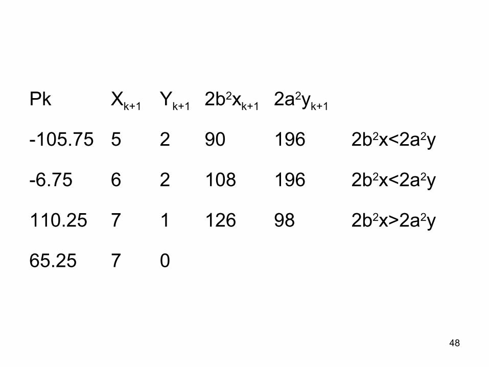
Pk Xk+1 Yk+1 2b2xk+1 2a2yk+1

-105.75 5 2 90 196 2b2x<2a2y

-6.75 6 2 108 196 2b2x<2a2y

110.25 7 1 126 98 2b2x>2a2y

65.25 7 0

48

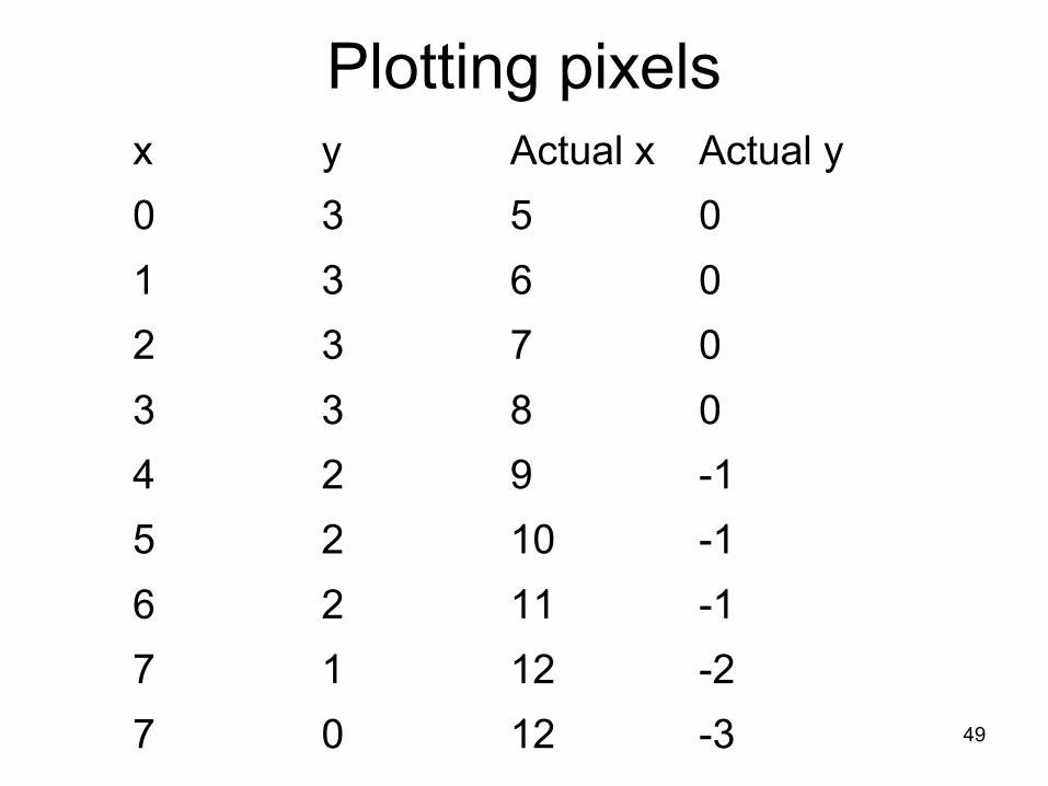
Plotting pixelsx y Actual x Actual y

0 3 5 0

1 3 6 0

2 3 7 0

3 3 8 0

4 2 9 -1

5 2 10 -1

6 2 11 -1

7 1 12 -2

7 0 12 -3 49

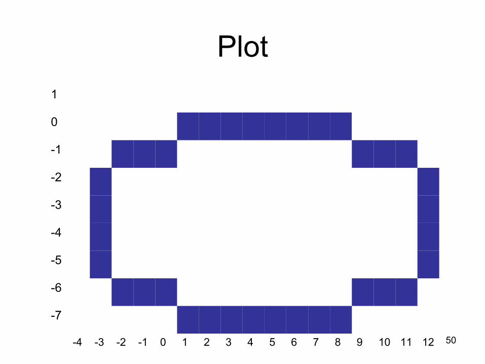
Plot

1

0

-1

-2

-3

-4

-5

-6

-7

-4 -3 -2 -1 0 1 2 3 4 5 6 7 8 9 10 11 12 50

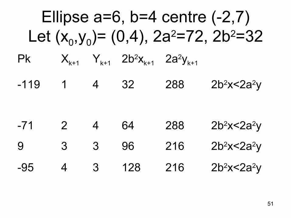
Ellipse a=6, b=4 centre (-2,7)Let (x0,y0)= (0,4), 2a2=72, 2b2=32

Pk Xk+1 Yk+1 2b2xk+1 2a2yk+1

-119 1 4 32 288 2b2x<2a2y

-71 2 4 64 288 2b2x<2a2y

9 3 3 96 216 2b2x<2a2y

-95 4 3 128 216 2b2x<2a2y

51

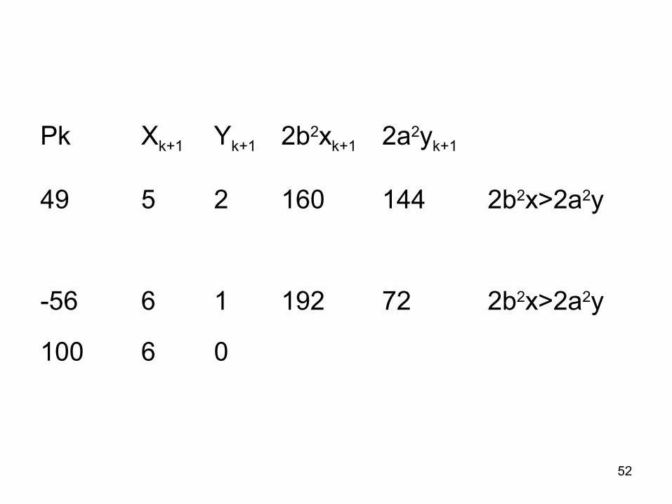
Pk Xk+1 Yk+1 2b2xk+1 2a2yk+1

49 5 2 160 144 2b2x>2a2y

-56 6 1 192 72 2b2x>2a2y

100 6 0

52

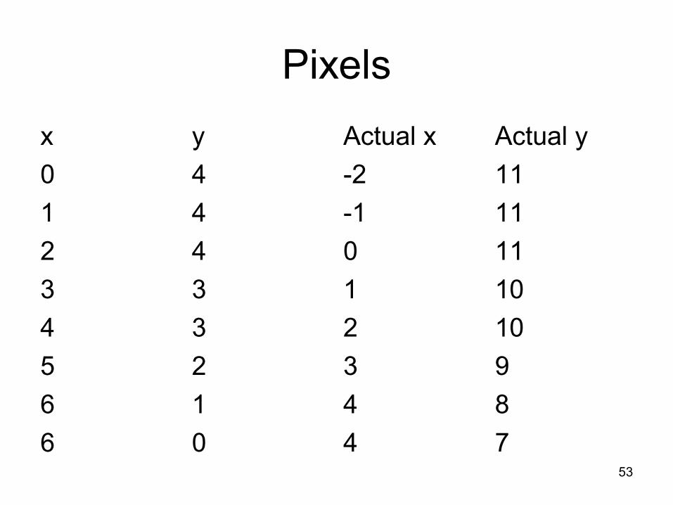
Pixels

x y Actual x Actual y

0 4 -2 11

1 4 -1 11

2 4 0 11

3 3 1 10

4 3 2 10

5 2 3 9

6 1 4 8

6 0 4 753

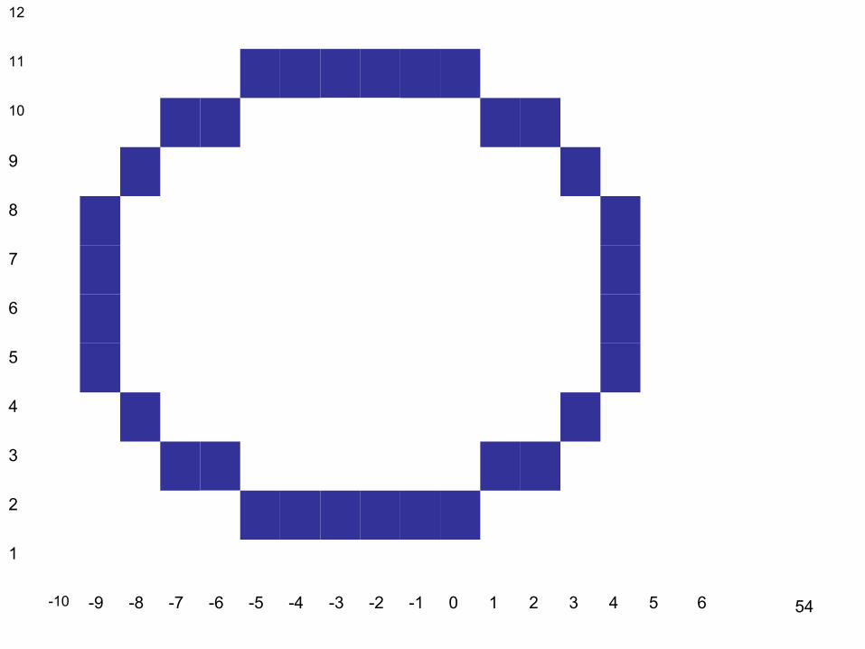
12

11

10

9

8

7

6

5

4

3

2

1

-10 -9 -8 -7 -6 -5 -4 -3 -2 -1 0 1 2 3 4 5 6 54

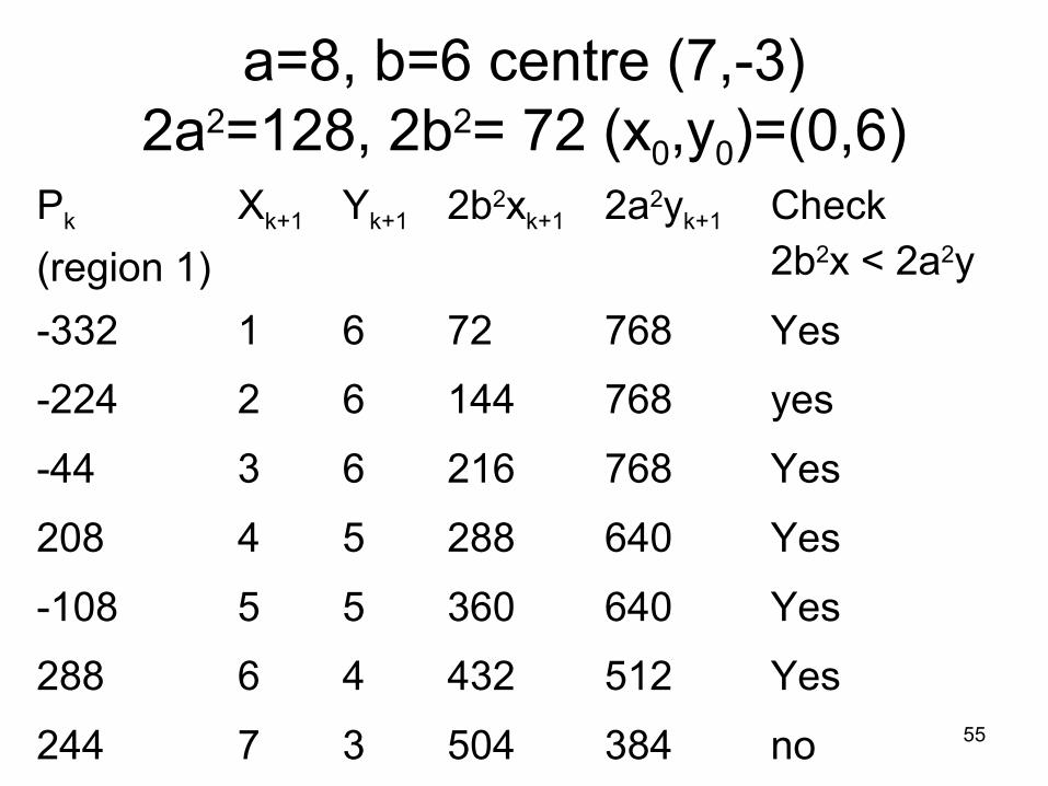
a=8, b=6 centre (7,-3)2a2=128, 2b2= 72 (x0,y0)=(0,6)

Pk

(region 1)

Xk+1 Yk+1 2b2xk+1 2a2yk+1 Check2b2x < 2a2y

-332 1 6 72 768 Yes

-224 2 6 144 768 yes

-44 3 6 216 768 Yes

208 4 5 288 640 Yes

-108 5 5 360 640 Yes

288 6 4 432 512 Yes

244 7 3 504 384 no 55

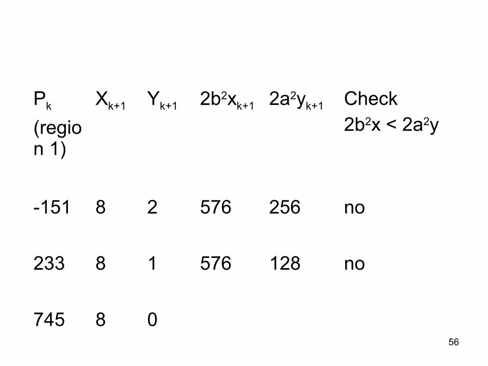
Pk

(region 1)

Xk+1 Yk+1 2b2xk+1 2a2yk+1 Check2b2x < 2a2y

-151 8 2 576 256 no

233 8 1 576 128 no

745 8 056

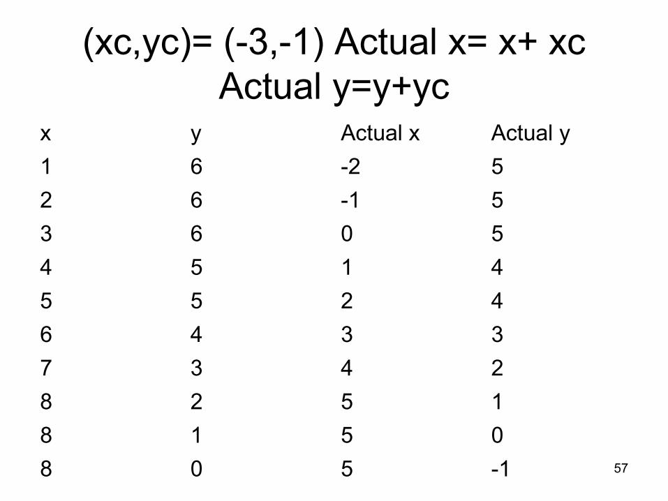
(xc,yc)= (-3,-1) Actual x= x+ xcActual y=y+yc

x y Actual x Actual y

1 6 -2 5

2 6 -1 5

3 6 0 5

4 5 1 4

5 5 2 4

6 4 3 3

7 3 4 2

8 2 5 1

8 1 5 0

8 0 5 -1 57

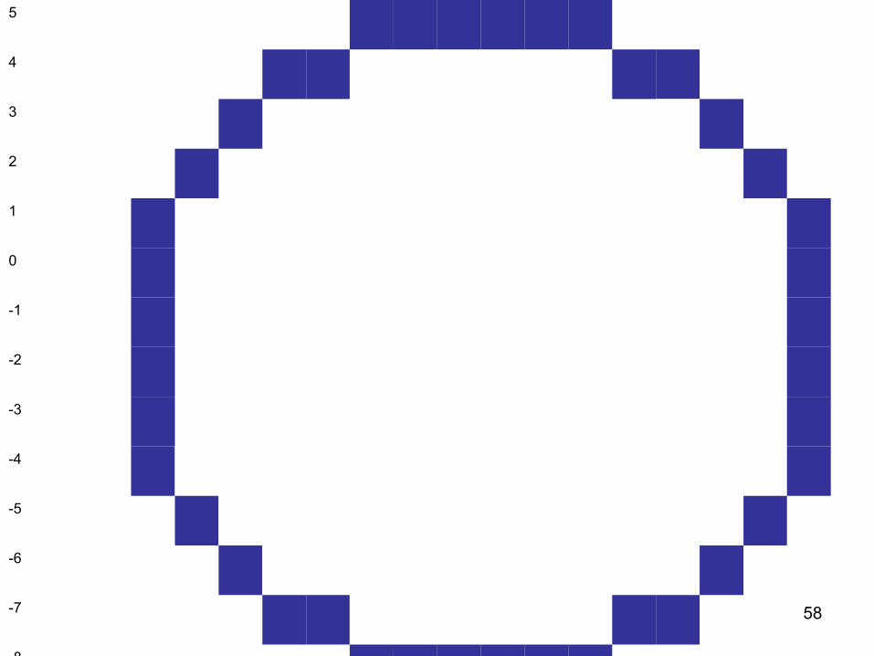
5

4

3

2

1

0

-1

-2

-3

-4

-5

-6

-7

-8

-12 -11 -10 -9 -8 -7 -6 -5 -4 -3 -2 -1 0 1 2 3 4 5 6

58

Filled area primitives

In graphics packages this is referred to as filled polygons.

• Scan line fill algorithm

• Boundary fill or flood fill algorithm.

59

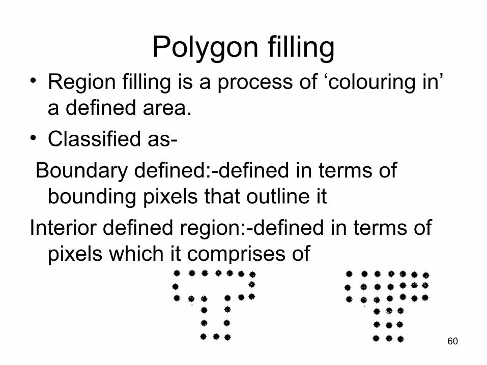
Polygon filling• Region filling is a process of ‘colouring in’

a defined area.

• Classified as-

Boundary defined:-defined in terms of bounding pixels that outline it

Interior defined region:-defined in terms of pixels which it comprises of

60

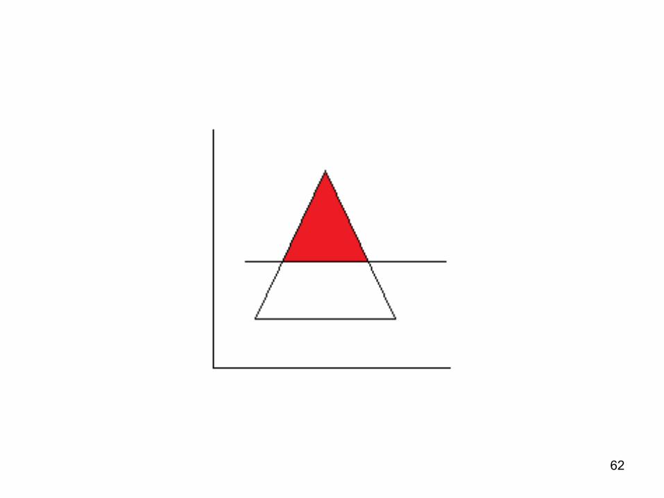
Scan line algorithm

• A scan line intersects a polygon at one or more points.

• For each scan line crossing a polygon, algorithm locates the intersection points of the scan line with the polygon edges.

• Intersection is considered in pairs.

• For interval between the pair of intersection, colour is that of background.

61

62

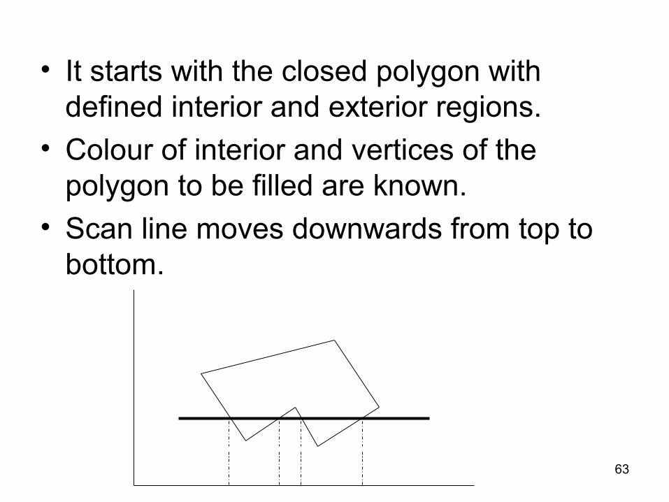
• It starts with the closed polygon with defined interior and exterior regions.

• Colour of interior and vertices of the polygon to be filled are known.

• Scan line moves downwards from top to bottom.

63

• For regular geometric figures, such as squares or rectangles, edges are well defined.

• Area can be filled directly by edge detection.

• Some polygons may requires special handling hen there are more than one intersection along the scan line.

64

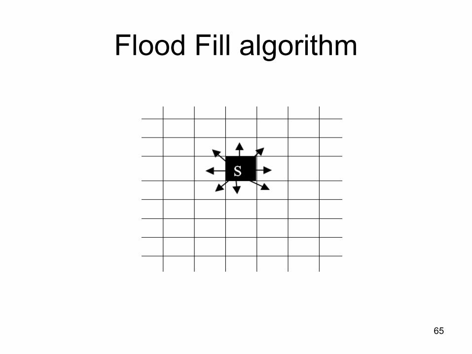
Flood Fill algorithm

65

• In flood fill algorithm user provides a seed pixel

• Starting from the seed pixel, algorithm will inspect each of the surrounding pixel to determine the extent of reach.

• Process is repeated until all pixels inside the region are inspected

66

• The seed pixel progresses recursively towards the boundary.

• If it encounters the boundary the chain terminates.

• The seed pixel enlarges to fill the area within the boundary.

• The enlargement of area and examining of neighbouring pixels can progress in two ways:

67

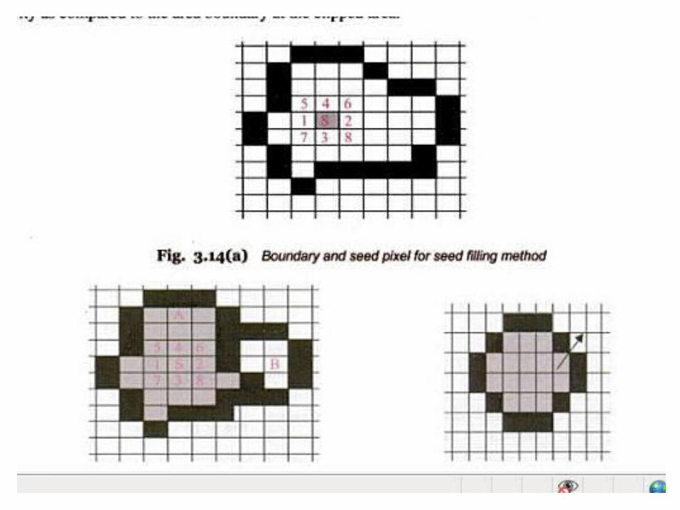
• Firstly to the four connected pixels, adjacent to it like right , left, bottom and top.

• Secondly through eight connected pixels including diagonal pixels.

• First way may fail to fill the complete area.

• Eight connected pixel is preferred.

• A curve or a circle leaves several diagonal pasages which prevents the application of boundary filling algorithm.

68

69

Scan line seed fill algorithm

• In seed fill algorithm, the stack size is very large.

• The duplicate pixels make the process slow.

• SLSF algorithm minimizes the duplicate pixels.

• Algorithm processes in raster pattern, along left to right in each scan line.

70

Flow of Algorithm

• A seed pixel located on the scan line is selected.• The line or span containing the seed pixel is

filled from left to right• including the seed pixel itself until the boundary

is found.• The extreme left and extreme right unprocessed

pixel in the span are saved.• The scan lines above and below the current

scan line are examined in the range of x-right and x-left.

71

THANKYOU

72