JOURNAL OF DIFFERENTIAL EQUATIONS 91, 355-388 (1991) Uniform Stabilization of a Nonlinear Beam by Nonlinear Boundary Feedback J. E. LAGNESE* AND G. LEUCERINC~ Department of Mathematics, Georgetown University, Washington, D.C. 20057 Communicated by Jack K. Hale Received November 20, 1989; revised March 20, 1990 1. PROBLEM FORMULATION AND STATEMENT OF MAIN RESULT We consider the planar motion of a uniform prismatic beam of length L. We want to derive a model that reflects the effect of stretching on bending, which necessarily leads to nonlinear partial differential equations for the motion of the beam. We will, however, assume that the constitutive equa- tions for bending are linear. This is in agreement with existing engineering literature (see, for example [S] and the bibliography therein). It should be remarked that the effect of stretching on bending becomes significant if, in particular, a rigid rotation is superimposed on the motion. We do not consider such a rotation here, even though it could be handled within the present framework. We assume that the beam, in its reference state, occupies the region described in rectangular coordinates by The line segment 0 <x< L, y = z = 0 is called the centerline of the beam, and the sets A(x)= ((x, y,z)) x=x,-l <y<l,--h/2<z<h/2} are its cross sections. Let r(x, t) denote the position vector at time t of the particle which occupies position (x, 0, 0) on the centerline in the reference configuration (so that r(x, t) - (x, 0,O) is the displacement vector of the particle). * Research supported by the Air Force Office of Scientific Research through Grant AFOSR 88-0337. + Research supported by the Deutsche Forschungsgemeinschaft. 355 0022-0396/91 $3.00 Copyright 0 1991 by Academic Press. Inc. All rights of reproduction in any form reserved

Welcome message from author
This document is posted to help you gain knowledge. Please leave a comment to let me know what you think about it! Share it to your friends and learn new things together.
Transcript
JOURNAL OF DIFFERENTIAL EQUATIONS 91, 355-388 (1991)
Uniform Stabilization of a Nonlinear Beam by Nonlinear Boundary Feedback
J. E. LAGNESE* AND G. LEUCERINC~
Department of Mathematics, Georgetown University, Washington, D.C. 20057
Communicated by Jack K. Hale
Received November 20, 1989; revised March 20, 1990
1. PROBLEM FORMULATION AND STATEMENT OF MAIN RESULT
We consider the planar motion of a uniform prismatic beam of length L. We want to derive a model that reflects the effect of stretching on bending, which necessarily leads to nonlinear partial differential equations for the motion of the beam. We will, however, assume that the constitutive equa- tions for bending are linear. This is in agreement with existing engineering literature (see, for example [S] and the bibliography therein). It should be remarked that the effect of stretching on bending becomes significant if, in particular, a rigid rotation is superimposed on the motion. We do not consider such a rotation here, even though it could be handled within the present framework.
We assume that the beam, in its reference state, occupies the region described in rectangular coordinates by
The line segment 0 <x< L, y = z = 0 is called the centerline of the beam, and the sets
A(x)= ((x, y,z)) x=x,-l <y<l,--h/2<z<h/2}
are its cross sections. Let r(x, t) denote the position vector at time t of the particle which occupies position (x, 0, 0) on the centerline in the reference configuration (so that r(x, t) - (x, 0,O) is the displacement vector of the particle).
* Research supported by the Air Force Office of Scientific Research through Grant AFOSR 88-0337.
+ Research supported by the Deutsche Forschungsgemeinschaft.
355 0022-0396/91 $3.00
Copyright 0 1991 by Academic Press. Inc. All rights of reproduction in any form reserved

356 LAGNESE AND LEUGERING
Assumption 1. The cross sections move rigidly; i.e., if p(x, y, z, t) is the vector describing the deformed position of the point (x, y, z), then p is determined by r(x, t) and two orthonormal vectors d,(x, t) and d,(x, t) through the formula
P(X, Y, z, 1) = r(x, t) + yd,(x, t) +4(x, t).
We set dl = d, x d,. The orthonormal system (d,, dl, d3) may be visualized as a moving coordinate system with d,(x, t) and d,(x, t) in the plane of the deformed cross section A(x); one has di = ei in the reference conliguration, where (e,, e2, e3) is the natural basis vor W3.
Assumption 2. The centerline is constrained to move in the e,e,-plane; i.e.,
r(x, t) = [u(x, t) + x]el + w(x, t)e,.
The quantities u and w represent, respectively, longitudinal and lateral displacement of the point (x, 0,O).
Under deformation of the beam, the point x on the centerline is mapped to a point P in the e,e,-plane whose abscissa is x + u and whose ordinate is w. The deformation causes an axial stretching s(x, t) within the beam that is given by the formula
~(x,t)=~~[(l+u’(~, t))2+(w’(5, t))2]1’2d4-x. (1.1) 0
The strains of the beam consist of six quantities. The first three are the components vi of r’ in the di basis (where ’ = a/ax); that is
ui=r’.di.
Assumption 3. There is no shearing of cross sections, i.e., v2 = v3 = 0.
The remaining three components of strain are related to bending and twisting motions and are defined as follows. Introduce the vector q by
dk=qxdk.
q exists and is unique since the dls form an orthonormal basis. The final three components of strain are the components of q in the di basis:
qi=q.di.
Components q2 and q3 measure the amount of bending about d2 and df, respectively, while q1 describes the amount of twist about d,. Assumption 2 implies that q3 = 0.
STABILIZATION OF A NONLINEAR BEAM 357
Assumption 4. There is no twisting about di : q1 = 0.
Any set of forces acting on the particular cross section located at x in the undeformed state can be replaced by a couple of torque T and a resultant force R such that
T = T,e, + M,e, + M3e3,
R=P,e,+ V,e,+ V,e,.
Here TI is an axial torque, Mi is a bending moment about e,, and Vi are the shear components of R. Assumption 3 requires that V, = V3 = 0, while Assumptions 2 and 4 require T, = M, = 0. Following [S] we have
P, = EAs’(x, t),
M, = -Elw”(X, t),
where the physical constants are A = 2h, the area of a cross section, I its moment of inertia with respect to the y-axis, and Young’s modulus E. EI is known as the flexural rigidity. (These are assumed to be constants only to simplify some of the computations below. This assumption is inessen- tial.) Therefore, the strain energy
can be expressed as
U= f l’ EA(s’)‘dx+ 4s” EZ(W”)~ dx. 0 0
From (1.1) we have
s’(x, t)= [(l +u’(& t))2+(w’(<, t))2]“2- 1. (1.2)
In order to obtain a reasonable simplification of s/(x, t), we use the first order approximation 1 + h/2 to the function Jl+h. We therefore replace the expression for s’ in (1.2) by
s’(x, t) = U’(X, t) + 4 (w’(x, t))2 + $ (u’(x, t))2.
In fact, we only take into account the first two terms in the last expression; i.e., we retain the quadratic term in the lateral strain while dropping the one in the longitudinal strain. This assumption is formally justified if the lateral displacement of the beam is supposed to be small with respect to its
358 LAGNESE AND LEUGERING
length. With these admittedly ad hoc assumptions, the strain energy takes the form
+!jL[,f+&,,‘)2]2dx+~jL(w”)2dx. 0 0
Following standard procedures, we find the kinetic energy to be
K=$jL(ti’)2dx++jL[(ti)2+(G)2]dx, 0 0
(1.3)
(1.4)
where . = a/at and p (assumed constant) is the mass density per unit volume of the beam in its reference configuration.
We define the Lagrangian density t(u’, w’, w”, ti, 6, IV) in terms of the densities 0, & of U, and K as
For the sake of simplicity, we neglect distributed body forces, and we assume the beam to be clamped at the left end; i.e., ~(0, t) = ~(0, t)= ~‘(0, t) = 0. We do, however, take into account forces acting on the right end. To be consistant with Assumptions 1 through 4, we assume that the resultant (with respect to y, z) end force n lies in the e,e,-plane,
n(t) = 4(t) e, + n2(t) e3,
and that the resultant moment of stresses is perpendicular to this plane,
m(t) =m,(t) e2.
Following Hamilton’s principle for contituous systems (see for instance [4]), we have to introduce variations of the field quantities u and w. As a necessary condition for the Lagrangian 9 to be stationary at U, w, the Gateaux derivative 69 of
9 = joT 5,” i(u’, w’, w”, zi, 6, if) dx dt
+ s T [n,u(L)+ n3 w(L) + m, w’(L)] dt 0
with respect to these variations must be zero. The appropriate spaces of variation are
H, = (24 Iz4EH’(O, L), u(O)=O},
H,=(wl w~H~(O,L),u(O)=w’(0)=0}.
STABILIZATION OF A NONLINEAR BEAM 359
We do not carry out the standard and straightforward calculation of 622 here. The result of the calculation is the following equations of motion and boundary conditions:
pAii - EA (24’ $4 w’2)’ = 0,
pA f,j - $,.$” + Ef,q”’ _ EA[w’(u’+; w’*)]‘=O,
u(0, t) = w(0, t) = w’(0, t) = 0,
EA(u’ + 4 w’~)(L, t) = n,(t),
EZw”(L, t) = -m2( t),
[ Elw”’ - ,aZtV - EAw’(u’ + 1 w’*)](L, t) = +I~(?).
In order to simplify notation, we introduce y* = Z/A and make the change t+tn. p E m the time scale. The above system is then brought to the form
G - (u’ + 1 w’2)’ = 0, $ _ y2i4u + y2w!/!I _ [w’(u’ + 4 w’2)]’ = 0,
u(0, t) = w(0, t) = w’(0, t) = 0,
To complete the description of the system, initial conditions are prescribed:
{u(O), W)} = {UO> 4, (w(O), W)} = {WO> w’> (0 <x < L).
In the new time scale, the strain and kinetic energies are given, respectively, by
u = 4 joL [y2w”2 + (24’ + 4 w’*)*] dx,
k2 + y%‘*) dx.
Remark 1.1. It is possible to obtain the same set of equations from a “first principles” approach in the flavor of [6, 11, thereby avoiding the
360 LAGNESE AND LEUGERING
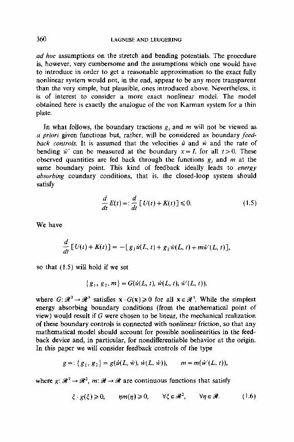
ad hoc assumptions on the stretch and bending potentials. The procedure is, however, very cumbersome and the assumptions which one would have to introduce in order to get a reasonable approximation to the exact fully nonlinear system would not, in the end, appear to be any more transparent than the very simple, but plausible, ones introduced above. Nevertheless, it is of interest to consider a more exact nonlinear model. The model obtained here is exactly the analogue of the von Karman system for a thin plate.
In what follows, the boundary tractions gi and m will not be viewed as a priori given functions but, rather, will be considered as boundary feed- back controls. It is assumed that the velocities zi and 6 and the rate of bending $’ can be measured at the boundary x = L for all t > 0. These observed quantities are fed back through the functions gi and m at the same boundary point. This kind of feedback ideally leads to energy absorbing coundary conditions, that is, the closed-loop system should satisfy
$qr)=:-$ [U(t)+K(t)] GO.
We have
$ CVf)+K(t)l= -Cgl4L, t)+ g,k(L, t)+mG’(L, t)],
so that (1.5) will hold if we set
where G: g3 + W3 satisfies x. G(x) 20 for all x E W3. While the simplest energy absorbing boundary conditions (from the mathematical point of view) would result if G were chosen to be linear, the mechanical realization of these boundary controls is connected with nonlinear friction, so that any mathematical model should account for possible nonlinearities in the feed- back device and, in particular, for nondifferentiable behavior at the origin. In this paper we will consider feedback controls of the type
g=: (g1, g2) = g(W, G)? *CL, @)I, m = m( ti’( L, t)),
where g: 92’ + W2, m: %? + W are continuous functions that satisfy
STABILIZATION OF A NONLINEAR BEAM 361
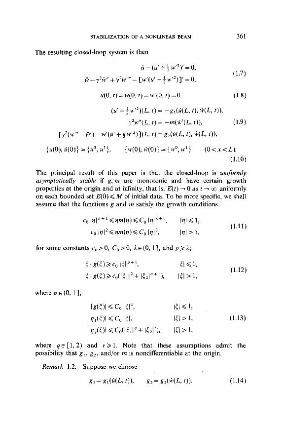
The resulting closed-loop system is then
fi - (u’ + 4 w’2)’ = 0, f+ _ y2+i! + y2wIIfI _
[w’(u’+$w’2)]‘=o,
u(0, t) = w(0, t) = w’(0, t) = 0,
(u’ + 4 w’2)(L, t) = -g,(ti(L, t), 3(L, t)),
y2w”(L, t) = -m(iJ’(L, t)),
[y2(w”’ - ti’) - w’(u’ + 4 w’2)](L, t) = g,(ti(L, t), G(L, t)),
(1.7)
(1.8)
(1.9)
{u(O), 40)) = {uO, u’>, {w(O), W,) = (wO, w’> (O<x<L). (1.10)
The principal result of this paper is that the closed-loop is uniformly asymptotically stable if g, m are monotonic and have certain growth properties at the origin and at infinity, that is, E(t) + 0 as t + cc uniformly on each bounded set E(0) < M of initial data. To be more specific, we shall assume that the functions g and m satisfy the growth conditions
co I~lp+‘~~m(~)6Col~I”+1, I?1 6 4
co 1912Gw(q)6Co h12, lrll > 1,
for some constants co > 0, Co > 0, A. E (0, 11, and p 2 A;
(1.11)
where 0~ (0, 11;
ls(Ol G co l51”?
lg1(01 G Gll51~
lgz(Ol G Co(15,14+ 152l’h
I51 G 1,
ICI > 1, (1.12)
I41 G 1,
I51 L= 1, (1.13)
I51 > 17
where q E [ 1,2) and r > 1. Note that these assumptions admit the possibility that g,, g,, and/or m is nondifferentiable at the origin.
Remark 1.2. Suppose we choose
g1= g,(W, t)), g2 = g,(*(L t)). (1.14)
362 LAGNESEAND LEUGERING
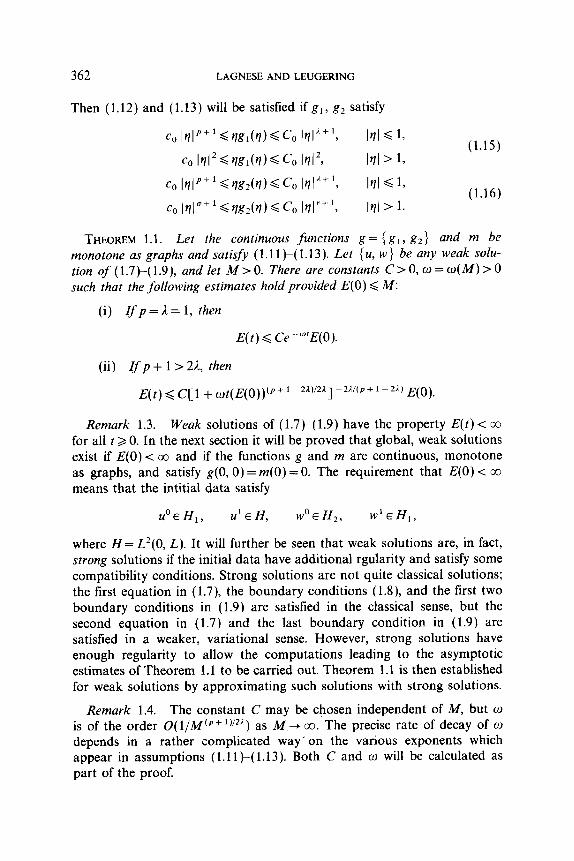
Then (1.12) and (1.13) will be satisfied if g,, g, satisfy
co Id p+‘Gqg2(rl)<co Wf’, Ill 6 13 (1.16)
co Irl u+1~vlg2(vl)~co lrlr+l, Id > 1.
THEOREM 1.1. Let the continuous functions g = {gl, g2} and m be monotone as graphs and satisfy (1.11 k( 1.13). Let {u, w ) be any weak solu- tion of (1.7)-( 1.9), and let M > 0. There are constants C > 0, o = o(M) > 0 such that the following estimates hold provided E(0) < M:
(i) Zfp=A= 1, then
E(t) d Ce-“‘E(O).
(ii) Ifp + 1 > 24 then
E(t) < C[l + wt(E(O))(P+’ P21)‘21] P2A’(P+1P21) E(0).
Remark 1.3. Weak solutions of (1.7)-( 1.9) have the property E(t) < GO for all t 2 0. In the next section it will be proved that global, weak solutions exist if E(0) < cc and if the functions g and m are continuous, monotone as graphs, and satisfy g(0, 0) =m(O) =O. The requirement that E(0) < co means that the intitial data satisfy
UOEHl, M’EH, WOE H2, w’EH,,
where H = L’(O, L). It will further be seen that weak solutions are, in fact, strong solutions if the initial data have additional rgularity and satisfy some compatibility conditions. Strong solutions are not quite classical solutions; the first equation in (1.7), the boundary conditions (1.8), and the first two boundary conditions in (1.9) are satisfied in the classical sense, but the second equation in (1.7) and the last boundary condition in (1.9) are satisfied in a weaker, variational sense. However, strong solutions have enough regularity to allow the computations leading to the asymptotic estimates of Theorem 1.1 to be carried out. Theorem 1.1 is then established for weak solutions by approximating such solutions with strong solutions.
Remark 1.4. The constant C may be chosen independent of M, but o is of the order 0(1/M (JJ + 1)/22) as A4 + co. The precise rate of decay of o depends in a rather complicated way’ on the various exponents which appear in assumptions (1.1 1 )-( 1.13). Both C and w will be calculated as part of the proof.
STABILIZATION OF A NONLINEAR BEAM 363
Remark 1.5. In the case p = A< 1, Theorem 1.1 gives a decay rate E(f)wt-2pl(1--P). Th is is in agreement with asymptotic estimates obtained in [3] for solutions of a cantilevered Euler-Bernoulli beam problem with nonlinear velocity feedback applied in the vertical shear force at the free end.
2. EXISTENCE AND UNIQUENESS OF SOLUTIONS
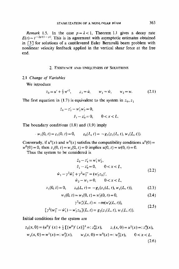
2.1 Change of Variables
We introduce
zo = u’ + $ w’2, Zl =ti, wl=s, w*=w. (2.1)
The first equation in (1.7) is equivalent to the system in zO, zi
i,-z;-w;w;=o,
i,-z;=o, O<x<L.
The boundary conditions (1.8) and (1.9) imply
w,(O, t)=z,(O, t)=O, zow, f) = -g,(z,(L t), Wl(L f)).
Conversely, if u”(x) and w’(x) satisfies the compatibility conditions u’(0) = w’(O) = 0, then z,(O, t) = w,(O, t) = 0 implies ~(0, t) = ~(0, t) = 0.
Thus the system to be considered is
z,-z;=w;w;, i,-zb=O, O<x<L,
k, - y2+; + y2w;ll = (w;z,)‘, (2.2)
G2-w,=o, O<x<L,
Zl(O, t)=O, zo(4 2) = -g,(z,W, t), w,(L, f)), (2.3)
w,(O, t) = w,(O, t) = wi(O, t) = 0, (2.4)
y2w;(L, t) = -m(w;(L, t)),
cY2(w; - %)- 4zolW, t) = g,(z,(L t), w,w, f)). (2.5)
Initial conditions for the system are
zo(x, 0) = (UO)’ (x) + 4 [(WO)’ (x)12=: z;(x), z,(x, 0) = u’(x) =: z?(x),
Wl(X, 0) = w’(x) =: w?(x), wz(x, 0) = w”(x) =: w;(x), O<x<L.
(2.6)
364 LAGNESE AND LEUGERING
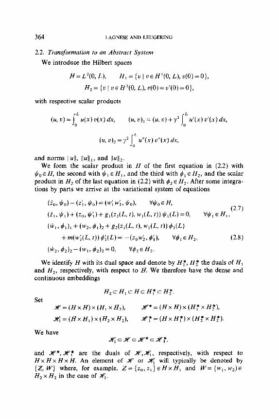
2.2. Transformation to an Abstract System
We introduce the Hilbert spaces
H = L*(O, L), H,={uI u~H’(O,L),v(0)=0},
H, = {II 1 u E H2(0, L), u(O) = u’(0) = 0},
with respective scalar products
(u, 0) = foL u(x)@) dx, (u, u), = (a, u) + y* joL u’(x) u’(x) dx,
(u, II)~ = y* foL u”(x) u”(x) dx,
and norms II4L IbIll, and Ib4112. We form the scalar product in H of the first equation in (2.2) with
$,, E H, the second with *I E H,, and the third with 4, E H2, and the scalar product in Hz of the last equation in (2.2) with #2 E H,. After some integra- tions by parts we arrive at the variational system of equations
(&I, $0) - (4 3 $0) = (4 4, Ii/o), Wo E H,
(i,, $1) + h II/i) + g,(z,(h t), WIW, t)) $,W) = 0, W1 EH1, (2.7)
(kl, hh + (w2,41)2 + g*(z,(L th w,(G t)) d,(L)
+m(w;(L t)) h(L)= -(%4, h), 475, ~ff2, (2.8)
(++2, $4212 - (WI, 42)2 = 0, 952 E H2.
We identify H with its dual space and denote by H:, H; the duals of H, and H,, respectively, with respect to H. We therefore have the dense and continuous embeddings
H,cH,cHcH:cH;. Set
X=(HxH)x(H,xH2), sP*=(HxH)x(H:xH;),
%=(HxH,)x(H,xH,), 2’: = (Hx H:) x (Hz x H;).
We have %Yqc~c2r*cJP:,
and X*, %?: are the duals of %,#r, respectively, with respect to H x H x H x H. An element of % or %, will typically be denoted by {Z, W} where, for example, Z= {z,,,z~}EHxH, and W= {wl, W*)E H2 x H, in the case of s.
STABILIZATION OF A NONLINEAR BEAM 365
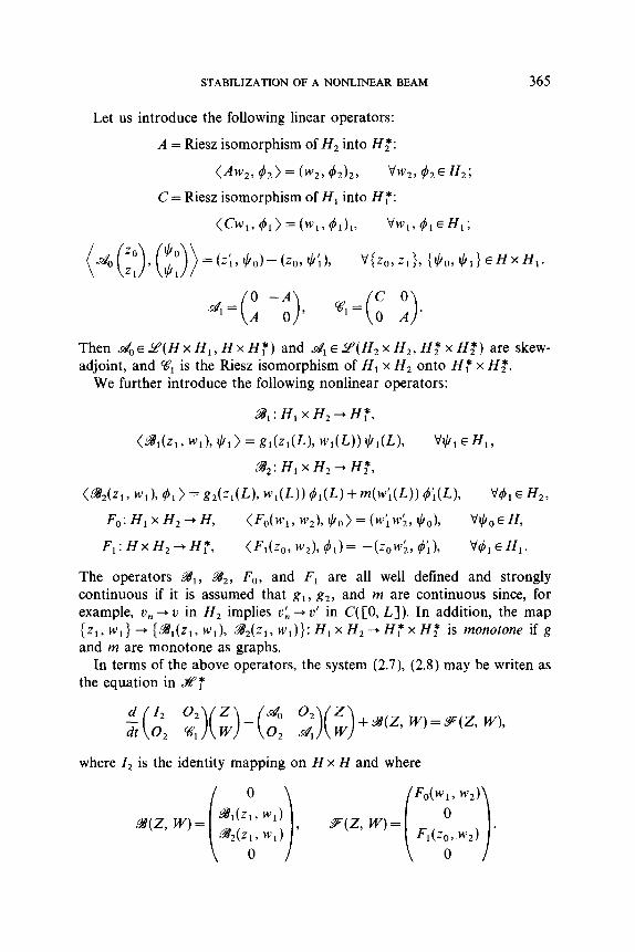
Let us introduce the following linear operators:
A = Riesz isomorphism of H, into HT :
(‘4% 42) = (wz, 4*)2, VW,, h~H2;
C = Riesz isomorphism of H, into Hf :
<cw,, 41) = (WI, 41)1, vw,,d,~H,;
= (z;? $0) - (zo, VI 13 Viz,, zd, {II/o, $11 EHXHI.
Then do~~(HxH1,HxH~) and dl~E(HzxHz,H:xH:) are skew- adjoint, and %‘i is the Riesz isomorphism of H, x H, onto H: x HT.
We further introduce the following nonlinear operators:
(%(Zl, WI), 46 > = g,(z,Wh w,(L)) d,(L) +m(w;w)) c&W), W ~ffz,
F,:H,xH,+H, (Fo(w, 7 wd $0) = (4 43 I(/o), Vo E H,
F,:HxH,+H:, <F,(zo, w,), 41)= +,w;, 4), ‘%EH~.
The operators B,, ?&, F,, and F, are all well defined and strongly continuous if it is assumed that g, , g,, and m are continuous since, for example, u, + u in H, implies u; + u’ in C( [0, L]). In addition, the map h w,} + {9ill(z1, w,), .!&(z,, wl)}: H, x H, -+ H: x H: is monotone if g and m are monotone as graphs.
In terms of the above operators, the system (2.7), (2.8) may be writen as the equation in .X:
where I, is the identity mapping on H x H and where
366 LAGNESE AND LEUGERING
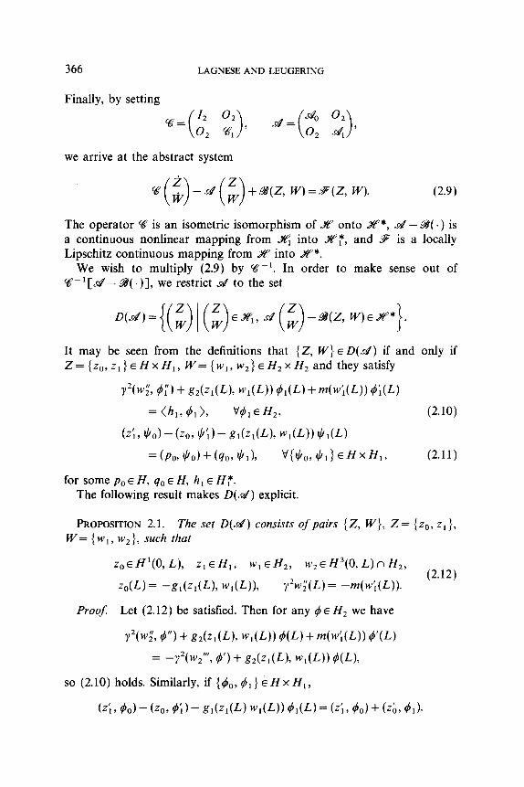
Finally, by setting
%=(;* g, d=(Z O&f),
we arrive at the abstract system
~(ii+o) + 93(Z, W) = F(Z, W).
The operator %? is an isometric isomorphism of X onto %?*, & - g( .) is a continuous nonlinear mapping from #i into A?:, and 9 is a locally Lipschitz continuous mapping from X into %*.
We wish to multiply (2.9) by g-‘. In order to make sense out of U-‘[&-&?(.)I, we restrict ~4 to the set
It may be seen from the definitions that (Z, W} E D(d) if and only if z= {zo, Z,}EHXH,, w= {WI, w2} E H, x H, and they satisfy
Y’(G 4;) + g*(zlw)~ WI(L)) 4,(L) +m(J4W,)) d;(L)
= <h,, #I>, WI ~H29 (2.10)
(4, $0) - (zch 9;) - g,(z,W), w,(L)) $1(L)
= (PO, $0) + (40, $I), v{$,, $11 EHxH,, (2.11)
for some p0 E H, q0 E H, h, E HT. The following result makes D(d) explicit.
PROPOSITION 2.1. The set D(d) consists of pairs {Z, W}, Z= (zO, z,}, w= {WI, w,}, such that
z,EH’(O,L), z,EH~, w,EH,, w2~H3(0,L)nH2,
z,(L) = -g,(z,W), W,(L))? y*w;(L) = -rn(w;(L)). (2.12)
Proof: Let (2.12) be satisfied. Then for any q4 E H, we have
Y2(G 4”) + g*(z1(~), w,(L)) cw) +44(L)) 4’(L)
= 4w2”‘Y 4’) + g*(z1(L), WI(L)) 4(L),
so (2.10) holds. Similarly, if { &,, b1 } E H x H, ,
(4, do)- (zo, K- g,(z,(L) w,(L)) 4,(L)= VI, hJ+ b&41).
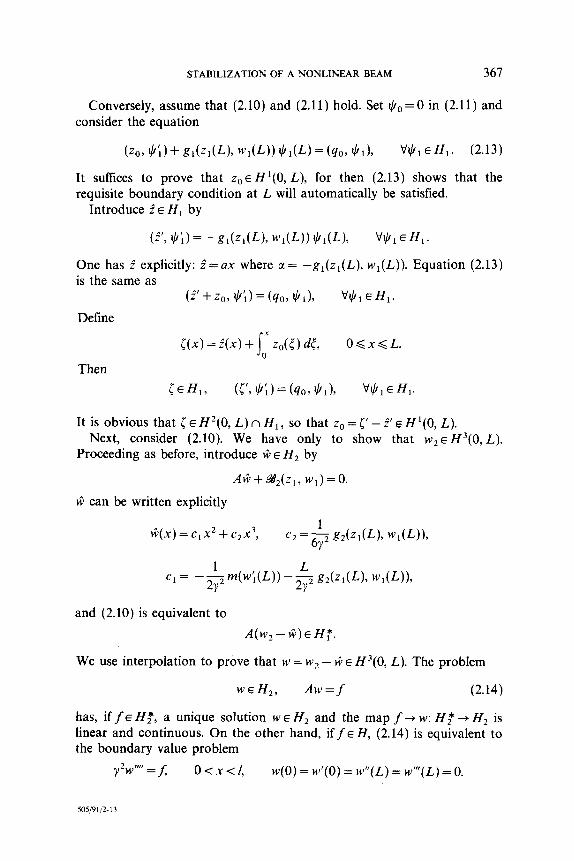
STABILIZATION OF A NONLINEAR BEAM 367
Conversely, assume that (2.10) and (2.11) hold. Set t+GO=O in (2.11) and consider the equation
(zo, ICI;) + gl(z,(L)T WI(L)) II/,(L) = (40, $I), b+bl E H,. (2.13)
It suffices to prove that z,eH’(O, L), for then (2.13) shows that the requisite boundary condition at L will automatically be satisfied.
Introduce i E H, by
(2’9 II/i) = -g,(z,(Lh w,(L)) b+,(L), W,EH,.
One has 1 explicitly: i= ux where CI = -g,(z,(L), w,(L)). Equation (2.13) is the same as
Define @‘+zo, fl)=(qo, $I)> WI EHI.
Then
It is obvious that i E H’(0, L) n H,, so that z0 = i’ - i’ E H’(0, L). Next, consider (2.10). We have only to show that WOE H3(0, L).
Proceeding as before, introduce 6 E H, by
AG++*(z,, w1)=0.
ti can be written explicitly
i(x)=c,x2+c*x3, c* =+ g*(z1(L), w,(L)),
Cl = -$wlw$2 g&1(L), w,(L)),
and (2.10) is equivalent to A(w, - G) E HT.
We use interpolation to prove that w = w2 - BE H3(0, L). The problem
w~Hz, Aw=f (2.14)
has, if fE HT, a unique solution w E H2 and the map f + w: H,* + H2 is linear and continuous. On the other hand, if f E H, (2.14) is equivalent to the boundary value problem
y2w”” = f, O<x<l, w(0) = w’(0) = w”(L) = w”‘(L) = 0.
505/91/2- 13
368 LAGNESE AND LEUGERING
The last problem has a unique solution w EH~(O, L) n H, and the map f + w: H--t H4(0, L) is linear and continuous. By interpolation, if f E [H, H:],,, = Hf’ then
WE CH4(0, L) n Hz, H211j2 = H3K4 L) n Hz,
and therefore w1 = w + ti, has the same property. 1
Remark 2.1. It follows from Proposition 2.1 that D(d) is dense in A“.
PROPOSITION 2.2. Assume that g and m are continuous, monotone as graphs, and g(O,O)=m(O)=O. Then W’[~-~Y(~)]:D(LZZ)CX-~ is maximal dissipative.
Proof: Let X= {Z, IV> and 8= (2, F} be in D(d). Then
(~-‘[~(x-8)-w(x)+~(X)],x-X),
= (d(X-X)-&Y)+W(X), X-X),*-,
= -(~(x)-~(x),x-x),r~,do
since d: S$ + SF? is skew-adjoint and %? is monotone. Thus W’[& - a( .)] is dissipative.
To show m-dissipativity, we have to prove that Range{l-W’[&--S9( .)] = S. Consider the equation
(2.15)
where Z={zO,zl}, W={wI,wz), P={p,,q,}, Q={h,,h,} withp,EH, qOEH, h,EH,, h,EH,. Equation (2.15) is the same as
(a,)( -~*)+wz, w++J.
The last equation is the same as the system
zo - 4 = PO,
w2-w1=h2, (2.16)
(zl,~l)+(zo1~;)+ <@l(Zl,Wl), Icl,)=(qo,$,), W, EHI,
(Cw,+Aw,,~,)+(~*(z,,w,),~,)=<Ch,,~,), WIEHZ. (2.17)
STABILIZATION OF A NONLINEAR BEAM 369
We use (2.16) to eliminate .a,, and w2 from (2.17) and thereby obtain the variational system
(2.18)
The mapping from H, x H, -+ H: x H: defined by
(Cw,+~w,,~,)+(z,,~,)+(z;,II/;)+(~,tz,,w,),II/,) + <%(ZlY WI), 41>, viti,> 4,) EHI xH2,
is monotone, continuous, and strictly coercive. It follows that (2.18) has a unique solution z1 E H,, w1 E H,. Retracing our steps, we have z0 = po+z;eH, w,=h,+w,~H, and
d Z
( > W -9qz, W)=‘&[( ;)-(;)p*.
Thus {Z, W}&(.&‘). 1
As a consequence of Proposition 2.2, and of Theorem 3.4 and Proposi- tion 3.3 of [2], we have the following result.
COROLLARY 2.3. Let the assumptions of Proposition 2.2 be satisfied, and let {Z’, W”} ED(&). Then there is a unique function t + {Z(t), W(t)}: [0, 00) + X such that
(i) {Z, W} is Lipschitzian on [0, a~));
(ii) {Z(t), W(t)} ED(~), t>O; (iii) (Z, W} is strongly right differentiable on [0, co); (iv) (Z, W} is weakly difSerentiable and { 2, I@} is weakly continuous
on (0, co );
qz+o) +B(Z, W)=Oon (0, co), {Z(O), W(O)} = {ZO, WO).
(2.19)
A continuous function t + {Z(t), W(t)}: [0, cc) + X with the properties (ii)- that satisfies (2.19) is called a strong solution of (2.19).
370 LAGNESE AND LEUGERING
2.3. Strong Solutions of the Inhomogeneous Problem Let us now consider the inhomogeneous problem
k-W[dX-a?(X)] =Jv”(X), X(0)=X0, (2.20)
where
x= (2, w>, N(X) = W’F(X).
The map N: 2 -+ Y? is continuous, M(O) = 0, and from the definition of B it is seen that JV is locally Lipschitzian. Thus, for every R > 0 there exists oR > 0 such that
IlJw7-JuY)II,d~. ID-- YIIXT vx, YEBR,
where RR(O) is the open ball in &’ of radius R centered at 0. Let X0 ED(&) be given and fix R > /IX’//,. Let NR be any globally
Lipschitzian function on 2 such that
JKdJ-1 = J-G7 on B,.
If We 2 oR denotes the Lipschitz constant for MR, we have
(-KQ(W - -4?(Y), x- Y), G OR IIX- Yll$,
and therefore &( .) - O,l is dissipative and Lipschitzian on #. It follows from [2, Lemma 2.41 that
is m-dissipative. Therefore, the problem
k=dJx)+W&r, X(0) = x0, (2.21)
has a unique solution X, = (Z,, W,} E C( [0, 00); 2) and X, has proper- ties (iik(iv) of Corollary 2.3 ([2, Theorem 3.171). Since -Pe, is dissipative and JJ&,(O) = 0, it follows from (2.21) that
so that
5 Ilxfdt)ll$ i OR W,(t)ll f,
IWR(t)ll 5 G e”Rt llX”Il f. (2.22)
Further, since R > IlX’ll,, it follows from (2.22) that there is a time r = z(R) = (i/OR) log(R/liX”l[,) such that
IWAt)ll~ < R on [0, 7).
STABILIZATION OF A NONLINEAR BEAM 371
But then Mj(X,(t)) = 1(X,(t)) on [0, r), therefore X, is a local strong solution of (2.20) on [0, r) and is, in fact, the unique strong solution there.
We next note that
Il~,Q(~)ll.2v d ll~“ll,? O<t<z. (2.23)
Indeed, X,(t) = {z,(t), zl(t), wl(t), wz(t)} satisfies (by its definition) the variational system (2.7), (2.8) for every t E [0, T). If we choose $a = z,(t), +I =zl(t), d1 = wl(t), and & = WI(t) and add the four equations in (2.7) and (2.8), we obtain the energy identity
;-$ Cllz0(t)l/* + llzI(t)l12 + Ilw)ll: + Ilw*(N:l
+ (.J%(z(t), w,(t)), z,(t)) + (~*(z1(t), w,(t)), w1(t)> =o,
that is, (2.23) holds. Let E > 0, E < r. Since the length of the interval [0, z) depends only on
the %-norm of the initial data (i.e., on R, which is a fixed number greater than ]lX”ll,), and since X,(z -E)E~(s/), we conclude from (2.23) that the unique strong solution on [0, r) may be continued as a strong solution to [z, 2r - E) 2 [t, 2(2 -E)]. By iteration, we obtain a unique strong solution X(t) of (2.20) on [O, n(t - E)] for every positive integer n.
Remark 2.2. The global strong solution X(t) of (2.20) is Lipschitzian on [0, T] for every T> 0, since X,(t) has this property.
We have proved the following result.
THEOREM 2.4. Let the assumptions of Proposition 2.2 be satisfied, and let {Z’, W”} ED(~). Th en there is a unique function t + {Z(t), W(t)}: [0, 00) -+ %’ such that
(i) {Z, W} is Lipschitzian on [0, T], VT>O;
(ii) {Z(t), W(t)) ED(~), t>O; (iii) {Z, W} is strongly right differentiable on [0, 00);
(iv) {Z, W} is weakly differentiable and (2, I@} is weakly continuous on to, 00 );
(v) (Z, W} satisfies (2.9) and {Z(O), W(O)} = {Z’, W’}.
Remark 2.3. It follows from Proposition 2.1 and Theorem 2.4 that, if {Z’, W”} ED(&), the strong solution {Z(t), W(t)) = {zo(t), zl(t), w,(t), w2( t)} described in Theorem 2.4 satisfies, for each T > 0,
ZE L”(0, T; H’(0, L) x H,), &Lrn(O, T;HxH),
WE L”(0, T; H, x (H3(0, L) n H2)), WE L”“(0, r; H, x H2),
zot4 t) = -g,(z,(L, t), Wl(L t)), y*w;(L, t) = -m(w;(L, t)).
372 LAGNESE AND LEUGERING
From (2.7), (2.8) we also conclude that
zo -z; = w; w;, i, - zb = 0, k,-w,=o,
(~~,~1)+Y2(~;~~;)-Y2(w~~~;)+g2(z1(L,~)~wl(L,~))$,(L)
= - ( zow;, 41, ‘@I ~ff2.
The last variational equation may clearly be extended to test functions d1 E HI. If we set w = w2, we obtain that {zO, z,, w} satisfy
i, - z; = w’k’, i, -zb=O,
(Gii, 41) + Y2(G’, $6) - Y2(WN’> 4) + g,(z,(L, .I, 44 .)I 4,(L)
= -bow’, qG), WI EHI.
Let US interpret the last remark in the context of the original initial- boudary value problem (1.7t(1.10). Let the initial data {uO, u’}, (w”, w’} be given, and let 2’ = {zt, zy>, W”= {WY, w;} be defined by (2.6). It is seen from Proposition 2.1 that the condition {Z’, W”} ED(&) is equiv- alent to
u’eH*(O,L)nH,, ~‘EH,, w”~ti3(0,L)nH2, w1~H2,
C(uO)’ + 1 ((w”Y)21(~) = -g,(u’(L), wl(Jw, (2.24)
y2(w0)” (L) = -m((w’)’ (L)).
Let {Z, W} be the unique strong solution of (2.9) with initial data {Z(O), W(O)} = {Z’, W”} ED(&), and define
4% t) = w,(x, t), 4x7 t) = jx Czo(5, t) - 4 (ML N21 &. 0
Then G= wi, u~L”(0, T; H*(O, L)n H,), tieLm(O, T; H,), and
2(x, t) =20(x, t) - wgx, t) wi(x, t) = z\(x, 2)
so that ti(x, t) = zi(x, t) + c(t). But ti(0, t) = z,(O, t) = 0, hence c(t) = 0. We therefore have the following result.
THEOREM 2.5. Let {u’, u’}, { w”, w1 } satisfy (2.24), and let g and m satisfy the conditions of Proposition 2.2. Then (1.7)-(1.10) has a unique strong solution (u, w} in the following sense:
I + {u(t), C(t)}: [0, T] + H, x H and t + {w(r), C(t)}: [O, T] + H2 x H, are Lipschitz continuous;
STABILIZATION OF A NONLINEAR BEAM 373
{u, ti) (resp., (w, w}) is strongly right differentiable and weakly differen- tiable on [0, co), and {ti, ii} (resp., {w, ti}) is weakly continuous;
UEL~(O, T, H2(0, L)nH,), ti E L-=(0, T; II,),
w E L”(0, F, H3(0, L) n Hz), G E L”(0, T); II,);
ii - (u” + w’w”) = 0, O<x<L, (2.25)
(G, 41) + y2(iv, qq) - $(w”‘, d)+ g*(w? .I, w+ .I) d,(L)
= -([u’ + 1 W’Z] w’, q&), w,Eff,; (2.26)
Cu’ + 4 (w’)*l(L, t) = -g,(W th WJ, t)), y2w”(L, t) = -m(G’(L, t)). (2.27)
2.4. Weak Solutions of the Inhomogeneous Problem
A function t + (Z(t), W(t)} : [0, co) -+ X is a weak solution of (2.9) if there is a sequence (Z,, W,} of strong solutions such that {Z,, W,} + {Z, W} in C(0, T; &?) for each T > 0. We will prove the following result.
THEOREM 2.6. Let g and m satisfy the conditions of Proposition 2.2. For every (Z’, W”} E 2, equation (2.9) has a unique weak solution such that {Z(O), W(O)) = {ZO, WO}.
Proof Let XE= {Zz, Wz} ED(~), Xg + X0= {Z’, W”} in X”, and let X,(t) = {Z,(t), W,(t)} be the unique strong solution of (2.9) with X,(O) = Xz. We have
xl(t) - L(t) - ~-‘C4Xn(t) - x,(t)) --@V,(t)) + wwm(t))l
= -ex”(t)) - Jwfm(t)),
and therefore
11x,(t) - x,,,(t)11 “, < j’ (eqx,(s)) - J(r(xm(s)), x,(s) - xrn(s)Lr d.7. 0
Let R > \IX’JI,. Then R> IIXjjlls for n>n(R). Since IIXn(t)llm < IlX$l, we have, with the notation of the previous subsection,
hence
11x,(t) - x,(t)ll$6 e”Rt IIXZ - X3l$.
Therefore, X,, + X in C(0, T; #), VT> 0 and X is, by definition, we weak solution of (2.9). It is clearly the case that 11X( t)ll x d llX”II *. If Y is also
374 LAGNESE AND LEUGERING
a weak solution such that Y(O)= Y” then, with R>max(IIX’I(,, I(Y’(I,), we obtain as above
11X(t) - Y(t)ll$ < PRf IIXO - YOll $, Vt20. 1
COROLLARY 2.7. Let g and m satisfy the conditions of Proposition 2.2, and suppose that
ZfOEH,, M’EH, WOE H,, w’EH,.
Then (1.7) - (1.10) has a unique weak solution with
{u,ti}~C([0,~);H,xH), (w,+}EC(CO, a);HzxHl).
3. PROOF OF THEOREM 1.1
It is sufficient to prove Theorem 1.1 for strong solutions since, if {u, w} is a weak solution, there is a sequence {u,, w,} of strong solutions such that E,(t) --f E(t) uniformly on [O, T] for every T> 0, where E,(t) is the total energy associated with the solution {u,, w,}.
We define
I‘&(t) =; [(ti(L, t))* + (G(L, t))* + y2(ti’(L, t))*],
U,(t) = g $(w”(L, t))2 + u’(L, t) +; (w’(L, t))* [ (
2
)I . The following energy identity plays a fundamental role in the derivation of the asymptotic energy estimates that follow.
LEMMA 3.1. Let {u, w} be a strong solution of (1.7~(1.9) and let T>O. For any DEB we have
p,(T)--p,(0)+jrj’ [(2a-5)ti2+(~+tx)).L2+y2(~-+V2]d~dt 0 0
++2a)(u’+$ w’*)*] dxdt
= I’ [JCL(t)- U,(t)] dt + Jrm(ti’(L, t))[Lw”(L, t) + aw’(L, t)] dt 0 0
T -
s g,(ti(L, t), C(L, t))[Lu’(L, t) + (1 - 20~) u(L, t)] dt 0
s
T -
g,(G, t), +(L, t))CLw’(L t) - CM& t)l 4 0
(3.1)
STABILIZATION OF A NONLINEAR BEAM 315
where
pm(t) = j; [x(tiu’ + Gw’) + y2bv(xw’)’
- a( wti + y2w%‘) + (1 - 2c() uti] dx. (3.2)
Proof. A strong solution has the properties delineated in Theorem 2.5 above. We multiply (2.25) by xu’ + (1 - 2cr)u and integrate the product over (0, L) x (0, T). Next, set 4I = xw’- CIW in (2.26) and integrate that equation in t over (0, T). Upon addition of the resulting two equations we obtain
o= joT joL ii(xu’ + (1 - 2a)u) dx dt + jOT jOL G(xw - c(w) dx dt
+ y2 jo= j; tY(xw’ - aw)’ dx dt
T - i.t L (u”+ w’w”)(xu’ + (1 - 2cr)u) dx dt 0 0
- IS
T L [y2wfll - w’(u) + f (w’)~)](xw’ - aw) dx dt 0 0
+ j’ g,(ti(L, t), +(I,, t))[Lw’(L, t) - aw(L, t)] dt. 0
(3.3)
We have
ii(xu’+(l-2a)u)dxdt
=PI(T)-P,(O)+ joTjoLfi2dxdt-;joTti2(L,t)dt, (3.4)
G(xw’ - aw) dx dt
=132(T)-t',(O)+ ;+a joTjoLk2dxdt-5 joTi+‘@, t)dt, (3.5) ( >
where
p,(t)= joLzi(xu’+(l-2a)u)dx,
p2(t) = joL ~(xw’ - c(w) dx.
376 LAGNESE AND LEUGERING
Also
B’(xw’ - aw)’ dx dt
=p,(T)--p,(O)+y’(a-;) joTjoL(kr)‘dxdt-$joT(ti’)‘(L,t)dt,
(3.6) with
P3(t) = Y2 joL tit’(xw’ - aw)’ dx.
Moreover,
w’w”)(xu’ + (1 - 2a)u) dx dt
i‘
T =- g,(zi(L, t), +(I,, t))[Lu’(L, t) + (l -2a) u(L, t)] dt
0
.T L -
J s [u’ + $ (w’)~](xu’ + (1 - 2a)u)’ dx dt, (3.7)
0 0 and
T L
SI w”‘(xw’ - aw)’ dx dt
0 0
s
T =- WZ(IV(L, t))(Lw”(L, t) - aw’(L, t)) dt
0
- y2 joT joL w”(xw’ - aw)” dx dt.
From (3.3 )-(3.8) we have
(3.8)
p,(T)-p,(0)+jTjL [(2a-i)ti2+($+a)G2+y2(a-$)N2] dxdt 0 0
+ jj T L[~‘+~(~‘)2][(~~‘+(1-2a)u)‘+w’(xw’-aw)’]dxdt 0 0
+y2joTi: w”(Xw’ - aw)” dx dt
= joT G(f) dt + joT m(vV(L, t))[Lw”(L, t) + aw’(L, t)] dt
- I oT g,(ti(L, t), ti(L, t))[Lu’(L, t) + (1 - 2a) u(L, t)] dt
s T - gM& t), 6% t))CLw’& t) - aw(L, t)l dt, (3.9) o
STABILIZATION OF A NONLINEAR BEAM 377
where
p,(t) = Pi(t) + P*(f) + h(t).
The last two terms on the left side of (3.9) still have to be calculated. For the last we have
y2 foT foL w”(xw’ - aw)” dx dt
=yzLjT(w”)*(L, t)dt+p2(;-a)j-T/L(~“)2dxdt. 0 0 0
As for the second term, it may be verified that
Therefore, the second and third terms in (3.9) may be written
joTjo’ ~(~-a)y~(w”)~+(f-2a)[u’+~(w’)~]~~dxdt+~~~U,(t)dt
which, when inserted back into (3.9) results in the desired identity. 1
Now fix an a E (l/2, 3/4) and set p(t) = p,(t),
Fe;,(t) = E(t) + wwww~ E > 0. (3.10)
fi will eventually be chosen as
p+l-21 B= 2L
(3.11)
but for the moment we keep b free, except that /I > 0. It will be proved that for E sufficiently small (depending on M),
Fe(t) 6 - $ (E(t))‘P+ 1m (3.12)
if p is given by (3.1 l), where k = min(2a - 1, 3 -4a). In what follows, C, Ci, C2, . . . . will denote generic constants which are
independent of E and M.
378 LAGNESE AND LEUGERING
From (3.10) we calculate
~~‘,(t)=~(t)+&~(t)(E(t))~+E~p(t)(E(t))~~’B(t),
and from (4.6)
(3.13)
But
s L
0 u”dx< ,‘[(u’+~~‘~)~+~u’~+,w’~]dx
s
so that
I L
u12dx<2 0
joL (u’ + 5 w’2)2 dx + C ( joL wN2 dx)2
Therefore
62 s oL [(u’+$~‘~)~dx+C(E(t))‘.
I P(t)1 G CCE(t) + (Jf3t))21 G cc1 + E(O)1 E(r).
Use of (3.14) in (3.13) gives
FE’,(t)< [l -@C(l +E(O))(E(O))q B(t)+qqt)(E(t))!
Next, b(t) is calculated using (3.1):
b(t)= -j-” [(2cr-l)ti2+(f+a)G2+y2(a-;)W2]dx 0
- s oL [y2($-a)w”2 + ($-2a)(u’+ f w’~)~] dx
+ KL(f) - U,(t) + m(3’(L, t))[w”(Zd, 2) + aw’(L, t)]
-s1(WL t))Chv, l) + (1-2a) 4L t)l
-g2( WG t))CLw’W, t) - au(L, t)l,
(3.14)
(3.15)
(3.16)
STABILIZATION OF A NONLINEAR BEAM 319
in which we have set W = {u, w }. Therefore
P(t)< -kE(t)+K,(t)-U,(t)+m(6’(L, t))[w”(L, t)-tuw’(L, t)]
-glvQ, t))CLu’(L f) + (l -2a) u(L, t)l
- g2( NL f))CLW’W, t) - au(G t)l, (3.17) where
k = min(2a - 1,3 - 4~).
We proceed to estimate the last three terms in (3.17), beginning with the third from last. In so doing, we shall write k, G’, u’, . . . . in place of ti(L, t), tt’(L, t), u’(L, t), . . . .
If IG’l< 1 we have
On the other hand, if [+‘I > 1, ,m(tv)(w” + aw’), 6 co ,6’, ,w” + aw’,
~~,~‘,*+C6(ur(r)+E(f))
~~~‘m(~‘)+C6(U,(t)+E(t)). 0
Therefore, we have for all k’ the estimate
Im(tV)(w”+aw’)l<$ x(liVl) l~~l~+~(l-X(l$‘o)ri’m(*‘)] [
+cs(u,(t)+E(t)), (3.18)
where x denotes the characteristic function of the interval [O, 11. We next estimate, for I I@ < 1, the quantity
Iowa’+ (l- 2@)U)l
(3.19)
380 LAGNESE AND LEUGERING
If [@i/l>1 we have
+*12+c~[Ur(f)+(1+E(0))E(c)]. (3.20)
From (3.19), (3.20) follows that for all I@,
I~,~~~~~u’+~~-22a~u~l~~cX~I~l~l~l~”+~1-X~l~l~I~l~1
Next, for I *I < 1, +CG(U,(t)+(l +E(O))E(t). (3.21)
Ig2(W)(Lw’-aw)l <g ~til*“+CM(t).
Let p E (0, 1). If I WI > 1 we estimate
ldww’-~w)l
(3.22)
co. . (fi” + w “2 I~~g(~)I’(ii2+~~+l)p
ILw’ _ aw,
(3.23)
We apply the inequality
(3.24)
(6>0, r> 1, s> 1, l/r+ l/s=l) to (3.23) with I= l/p, s= 1/(1-p) in order to obtain
+c2dP’/(l-P) [l~~(4-2~c)/(l-~)+I~~(r~~(o+1))/(1-~)1
x JLW’ -awl l/(1- p). (3.25)
STABILIZATION OF A NONLINEAR BEAM 381
We require ,U <q/2 and apply (3.24) to (ti((q-21r)‘(1-P) lLw’- awl ‘A-~) with r = 2( 1 - p)/(q - 2~), s = 2( 1 - ~)/(2 - q) to obtain the estimate
lfil(q-*P’)/(l-P) I~w’-clwll/(l-P)
G&2+ Iti,*+& ,Lw’-crwl*“*--y)
In addition,
< C[ hf. g(W) + (E(t))“‘*--y)] < C[ ri/. g( i-v) + (E(0))(q-‘)‘(2-Q)] E(t). (3.26)
< C(E(O))(‘~‘~~‘(‘-“))/*(‘-iU) E(t) (3.27)
provided p < (r - 1 )/( 1 - 0). (We may assume that r > 1 without loss of generality.) It follows from (3.25)-(3.27) that for 16’1 > 1,
Ig2(?@)(Lw’-aw)l <$l rP.g(ci/‘)+c26~‘(1-fl)
x [(E(()))(4-1)/(2- ) 4 + (q()))“- l-L41 ~dM--P)] E(t),
(3.28) where 0 < P-C min(q/2, (r - 1 )/( 1 - a)).
The combination of (3.22) and (3.28) yields that for all I@,
Ig,~~)(Lw’-orw~l~~X(l~l) Iril*~+~(l-x(l~l) bv.g(Jei/) +c2y+q1 +(q)))(q-‘M-4) +(~(O))(‘-l-‘(l~u))/2(1-~‘)] qt), (3.29)
if we also require that CL< l/2. It follows from (3.17), (3.18), (3.21), and (3.29) that
382 LAGNESE AND LEUGERING
We substitute (3.30) into (3.15) and obtain an estimate of the form
&(t) d Cl -EPC(l +E(O))(E(O))q B(r)
-&{k-C1w-ql +E(O)+ (E(o))(~-J)‘(2pq) +(E(o))“-J~~‘“-J,U~‘J-~)]}(E(~))B+J
+ 4E(t))B i
&(I) - (1 - C,(3) U,(f)
+g[x(lwl) Itii/l’“+x(Itvl) Jti’12”]
+$J[(1-X(l~l)(bv-g(Fv)+lkl2)+(1-X(l~~l)ll’m(J.)1},
(3.31)
Since k(ct) = - ci/. g( I$‘) - k’m(G’) we may deduce from (3.31) that
&t) < Cl - $C(l + E(O))(E(O))“I B(t)
-E{~-C~~“‘(~~~)[~+E(O)+(E(O))(~-~)’(~-~)
+ (E(O))(‘-‘-“(6-‘))/2(‘.-“) 1 kW))B+l -4E(t))’ (1 - C26) u,(t)
+4E(t))P K,W+$(l-x(lfil) 1*12)] [
++WB Cx(l*l) I~l’“+xWl) I~‘l*“l. (3.32)
We next estimate the last term in (3.32), assuming that p + 1 > 211. The other possibility p = L = 1, which is simpler, is left to the reader.
We have
(EO))B~O~l) I*l’”
& ~.g(Ci/‘)+C212~i(P+l~21)(E(1))B(P+l)/(P+’~2~), ?
(3.33)
where r] > 0 is arbitrary. Similarly,
STABILIZATION OF A NONLINEAR BEAM 383
If (3.33) and (3.34) are substituted into (3.32) there results
Fe(t)< 1 -&flC(l +E(0))(E(O))P--~(E(O))P-~ [ 1 k’(t)
-&{k-C16Y’(1-“)[1 +E(O)+(E(O))‘Y~““*-Y’
+ (~(O))(‘~‘~~‘(~-‘))/*(‘~~‘) 1}(Jw)“+’ -@(t)P (1 - C26) U,(t)
+EC,)12il~p+l~2~~(E(t))P~~+l~!~~+121)
6
+&(E(t))~ K,(t)+$(l-X(lPl) WI’) [ 1 . (3.35)
To estimate the last term in (3.35) the two possibilities J.-C p G 1 and p > 1 will be considered separately.
Suppose that p< 1. Since then ItI*< l~lP” for 151 < 1, it follows from (1.11) and (1.12) that
(E(t))fi [l~12+l~‘12]~[I~~+1+l~‘(2](E(0))~
~‘[w.g(bv)+Jvn7(bv)](E(O))~ CO
for all k’ and for I L&l < 1. If I I@[ > 1, we have
(3.36)
Therefore, for I WI > 1,
(E(t))B , WI2 GF w. g(W) + C,@yE(t))fl+(“+ ‘wJ 0
pw~ * cy] w. g( kv) + c,~""(E(o))"-""*" (J?qt))~+l.
0
505/91/2-14
384 LAGNESE AND LEUGERING
We conclude that if p < 1, the last term in (3.35) is bounded above by
l/c =$ (E(O))fl B(t) ++ (E(o))(1-o)‘2c (E(t))fi”,
where C,, C, are independent of E(O), 6, and rl (if 6 < 1 and q < 1). If, therefore, p < 1 we obtain an estimate of the form
&(t)< 1 -E/x(1 +E(O))(E(O))“-2(1 +(J?(O))b) B(t) [ 1 --E k-C16~“1-P’[1+E(0)+(E(0))‘q-1”‘2-q’
{
+(E(0))“~l~~~“-l”/“l-“‘]~c,~(E(O))”~””’”
1 (E(t))‘+’
+~?2~/(P+1~2i)(E(t))B(p+lJ;llc’-21)--E(E(t))B(l -C2a) u,(t).
(3.37) Now assume that p > 1. The last term in (3.35) may be written
+y2x(I+iq) Iti’l’+y’(l-~(l~‘l)) Iti’ . 1 (3.38)
By estimating in the same manner as in (3.33) we obtain
4E(t))BCxU~l) I~12+~2xW’l) WI’1
<c’ [~.g(~)+~‘m(~‘)]+C2~2/(“--)(E(t))~(p+1)~(p--). ?
(3.39)
On the other hand, the term (1 - x( I WI)) 1 ci/l 2 may be estimated as in (3.36). Therefore, if p > 1 we conclude that
(E(t))’ &W++x(l@N Iw12] [
<z (1 + (E(0))8)( w. g( I@)+ tihn(~+‘))
+C2~2/(P-1)(E(f))B(P+l)/(P--1)+ y (E(,,))“-“‘/2” (E(t))fl+ 1.
(3.40)
STABILIZATION OF A NONLINEAR BEAM 385
Substitute (3.40) into (3.35) to obtain an estimate that has the structure
&(t)< [
1-&pc(l+E(o))(E(o))~-$l+(E(O))P) k(t) 1 -& k-C,6~“‘-“‘[1+E(O)+(E(0))‘4-““*~q’
{
+ (E(o))“- 1 -Au- l)Ml -q _ c, q (E(O))” -fJlPa I
bW))B+l
-E(E(~))~ (1 -C26) UL(t)+~Cqy12’(P-‘)(E(f))B(p+1)‘(p--1)
+EC5~*i/(P+l-*1)(E(t))P(P+l)!(P+l-*I). 6
(3.41)
The estimate (3.12) is obtained from (3.37) or (3.41), depending on whether p < 1 or p > 1. We consider the case p > 1 and leave it to the reader to provide the minor changes needed to treat the opposite case.
So far p>O has been arbitrary. We now choose /I so that
RP + 1) p+l-211
=/I+l,
that is, /I = (p + 1 - 2A)/2A. Then
We may therefore combine all the different powers of E(t) in (3.41) and we arrive at the estimate
&(t)< l-&~C(l+E(0))(E(O))R~(l+(E(O))~) i(t) 1 --E k-C,6fi”‘-~“[1+E(0)+(E(0))‘q-1”‘2~q’
{
+(E(O))(‘-‘-~““~‘))/*(l-~)] -C4r12/(P-1)(E(0))(l~I)(P+I)/l(P--l)
- c$ (E(0))“p”‘/2”} (E(t))fl+ 1
-E(E(~))~ (1 - C,6) U,(t). (3.42)
386 LAGNESE AND LEUGERING
Case 1. p=l= 1. Then p=O and (3.37) reduces to
Fe(t)< l-2 B(t) ( > --E k-C,6~“1P~‘[1 +E(O)+ (E(0))(Y-‘)‘(2PY)
1
+ (~(O))(‘-l-~(u~l))/*(l-~‘)] _ C6T (q()))w)/*o
> E(f)
-E(l -C,(5) U,(t). (3.43)
Suppose E(0) < M. Choose 6 > 0 so small that
1 k d<- k-C16”/(‘-~‘)[1+M+M(4-1)/(*-4)+Mr-I-~(u~1))/*(1--a)]~-. C2’ 4
Having selected 6, choose q > 0 so small that
With 6 and q chosen, pick E > 0 so small that
1-S>O. drl
We then obtain
(3.44)
From (3.10) (with p=O) and (3.14) we have
IFAt) - E(t)1 < d’(1 + M) E(t)
so that
and
[l-&(1 +M)] E(t)dF,(t)< [l +&C(l +M)l E(t) (3.45)
&(t)< - Ek
2[1 +eC(l +M)] Fe(t)
=: - oF,( t).
STABILIZATION OF A NONLINEAR BEAM 387
Therefore
SO that, if
F,(t) < eC”‘F,(O)
1 EiC(l +44)’
we have
[l +eC(l +A4)] ~ E(t) d c1 _ Ec(l + M), e “‘JW),
ck m=2[1+EC(1+M)].
(3.46)
Case 2. p + 1 > 21. We choose 6 as in Case 1, and then choose q so that
With 6 and q chosen, let E > 0 satisfy
Since, in this case,
IF,(t)-E(t)1 <EC(l +M) M”E(t)
we obtain
< -$ [l +EC(l +M)M”]-a-’ (F,(t))@+’
=: -K(F,(t))~+‘,
which, upon integration, yields
(3.47)
(FE(t))p G (Fe(O))’ 1 + (Fe(O))8 KBr’
Since
(Fe(O))8 < (E(O))8 [ 1 i- EC( 1+ M)M”] p
388
we have
LAGNESE AND LEUGERING
(F8(t))B G [ 1 + EC( 1 + M) A4q B (E(O))B
1 + (&/2)(E(O))fi [ 1 + EC( 1 + M) W] P1 fit
and therefore if 1 - EC( 1 + M)Mp > 0,
E(t) < z’[l + wt(E(O))q -l/P E(O), P= p+l-2A.
2il >
where
&l+EC(l+M)Mfl EkB l-EC(l+M)MB’ w=2[1 +&C(l +M)Mq’
Remark 3.1. Since~<l/C(l+M)MB,itisseenthato+OasM-+co at least as fast as Mec8+ ‘). On the other hand, by insisting that E < 1/2C( 1 + M)MB (for example), we may bound c independently of M.
ACKNOWLEDGMENT
The authors thank E. Zuazua for helpful comments on an earlier draft of this paper that allowed some weakening of assumptions (1.11) and (1.12).
REFERENCES
1. S. S. ANTMAN, Theory of rods, in “Handbuch der Physik, Via,” Springer-Verlag, Berlin, 1972.
2. H. BREZIS, “Operateurs Maximaux Monotones,” North-Holland, Amsterdam, 1973. 3. F. CONRAD, J. LEBLOND, AND J.-P. MARMORAT, Energy decay estimates for a beam with
nonlinear boundary feedback, “Proceedings of the COMCON Workshop on Stabilization of Flexible Structures, Montpellier, France, January, 1989.”
4. H. GOLDSTEIN, “Classical Mechanics,” Addison-Wesley, London, 1980. 5. T. R. KANE, R. R. RYAN, AND A. K. BANERJEE, Dynamics of a beam attached to a moving
base, J. Guid. Control Dyn. 10 (1987). 6. R. C. ROGERS AND D. L. RUSSELL, Derivation of linear beam equations using nonlinear
continuum mechanics, preprint.
Related Documents