Underwater Sensor Networks: The physical layer

1

Underwater Sensor Networks:The physical layer

Short tutorial on the physics of sound in underwater environments.

Jens M. HovemScientific Advisor SINTEF-ICT

Professor emeritus NTNU [email protected]

Sensorcom2009 Athens

2

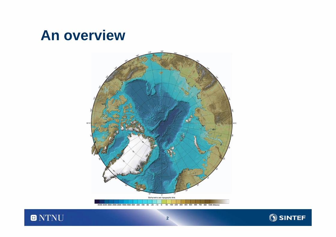
An overview

3

Applications of Marine Acoustics

• Military applications and surveying of coastal areas, vessels and mines.• Fishery acoustics and abundance estimation of fish and plankton.• Sea floor acoustics, hydrography and mapping of the topography and structure of the

sea floor and sub-bottom. • Underwater communication • Underwater navigation and position reference systems.• Acoustic remote sensing of the oceanic conditions.

4

Issues in Acoustic Underwater Communication

Low data rates: Bandwidth limitations, absorption, noise.Channel characteristics: Range (time) and frequency shift (Doppler). Coherence degradationOceanic variability: Significant problem, but the seriousness dependent on positions of the nodes.Transmitters/receivers: No standards (jet) and limited availability.

5

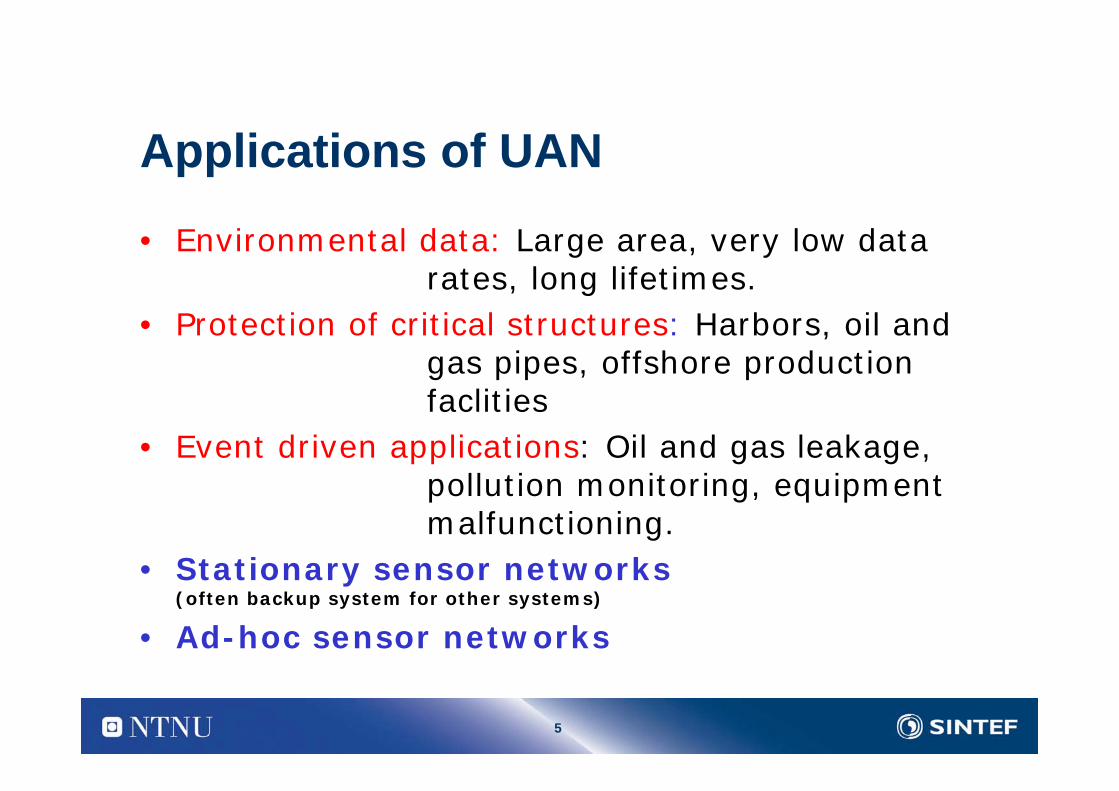
Applications of UAN

• Environmental data: Large area, very low datarates, long lifetimes.

• Protection of critical structures: Harbors, oil and gas pipes, offshore production faclities

• Event driven applications: Oil and gas leakage, pollution monitoring, equipment malfunctioning.

• Stationary sensor networks (often backup system for other systems)

• Ad-hoc sensor networks

6

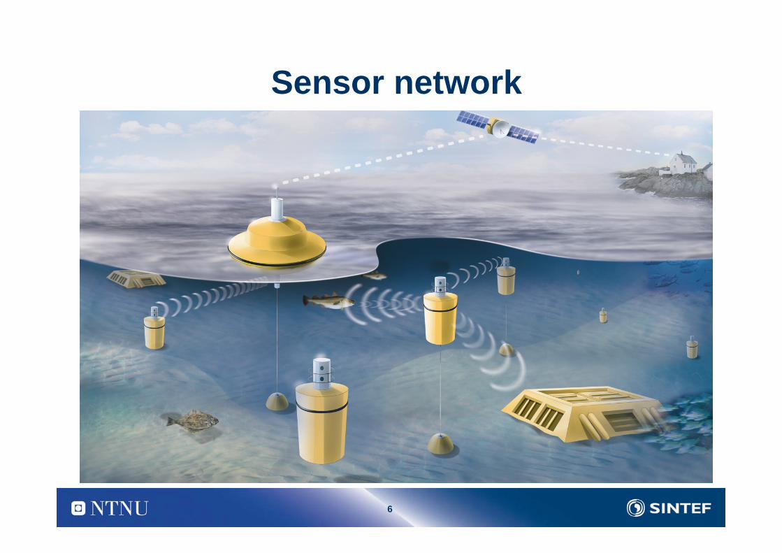
Sensor network

•

7

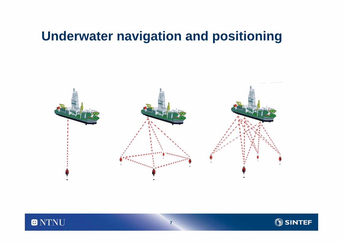
Underwater navigation and positioning

8

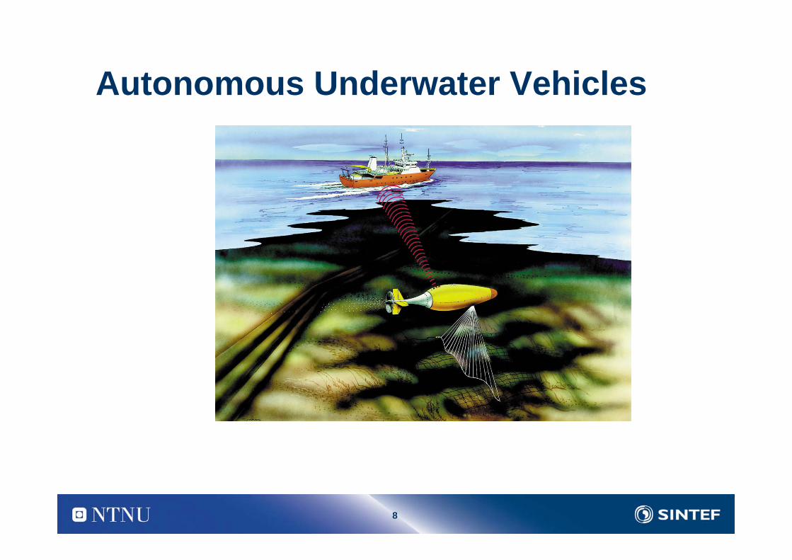
Autonomous Underwater Vehicles

9

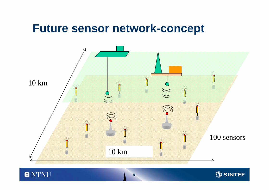
Future sensor network-concept

10 km

10 km

100 sensors

10

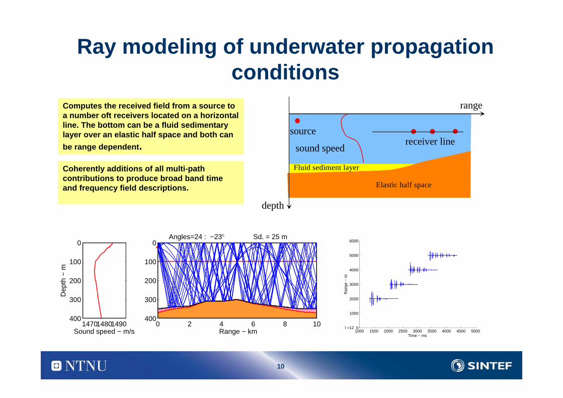
Ray modeling of underwater propagation conditions

depth

range

sound speed

sourcereceiver line

Elastic half space

Fluid sediment layer

1.Computes the received field from a source to a number oft receivers located on a horizontal line. The bottom can be a fluid sedimentary layer over an elastic half space and both can be range dependent.

147014801490

0

100

200

300

400

Sound speed − m/s

Dep

th −

m

0 2 4 6 8 10

0

100

200

300

400

Range − km

Angles=24 : −23° Sd. = 25 m

1000 1500 2000 2500 3000 3500 4000 4500 50000

1000

2000

3000

4000

5000

6000

I =12

Time − ms

Ran

ge −

m

1.Coherently additions of all multi-path contributions to produce broad band time and frequency field descriptions.

11

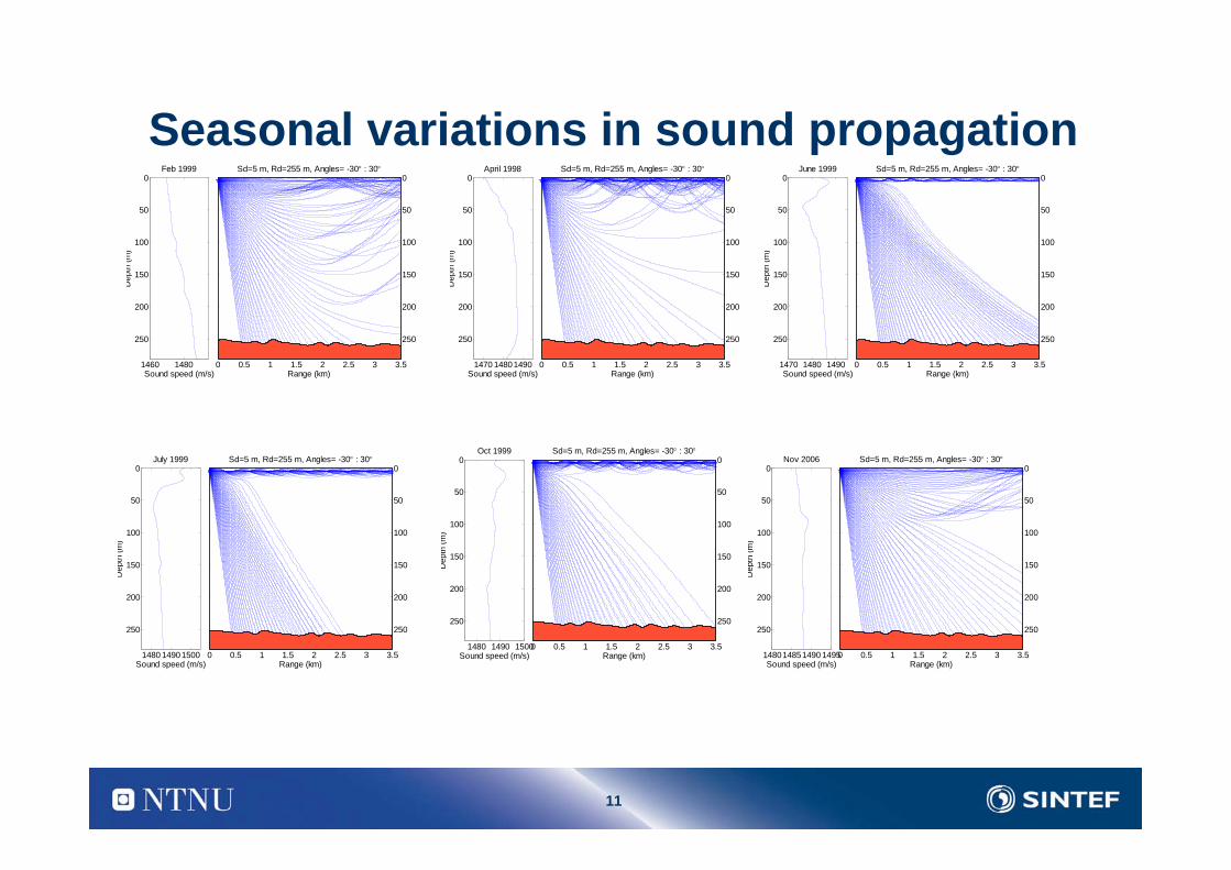
Seasonal variations in sound propagation

1460 1480

0

50

100

150

200

250

Sound speed (m/s)

Dep

th (m

)

Feb 1999

0 0.5 1 1.5 2 2.5 3 3.5

0

50

100

150

200

250

Range (km)

Sd=5 m, Rd=255 m, Angles= -30° : 30°

1470 14801490

0

50

100

150

200

250

Sound speed (m/s)

Dep

th (m

)

April 1998

0 0.5 1 1.5 2 2.5 3 3.5

0

50

100

150

200

250

Range (km)

Sd=5 m, Rd=255 m, Angles= -30° : 30°

1470 1480 1490

0

50

100

150

200

250

Sound speed (m/s)

Dep

th (m

)

June 1999

0 0.5 1 1.5 2 2.5 3 3.5

0

50

100

150

200

250

Range (km)

Sd=5 m, Rd=255 m, Angles= -30° : 30°

1480 14901500

0

50

100

150

200

250

Sound speed (m/s)

Dep

th (m

)

July 1999

0 0.5 1 1.5 2 2.5 3 3.5

0

50

100

150

200

250

Range (km)

Sd=5 m, Rd=255 m, Angles= -30° : 30°

1480 1490 1500

0

50

100

150

200

250

Sound speed (m/s)

Dep

th (m

)Oct 1999

0 0.5 1 1.5 2 2.5 3 3.5

0

50

100

150

200

250

Range (km)

Sd=5 m, Rd=255 m, Angles= -30° : 30°

148014851490 1495

0

50

100

150

200

250

Sound speed (m/s)

Dep

th (m

)

Nov 2006

0 0.5 1 1.5 2 2.5 3 3.5

0

50

100

150

200

250

Range (km)

Sd=5 m, Rd=255 m, Angles= -30° : 30°

12

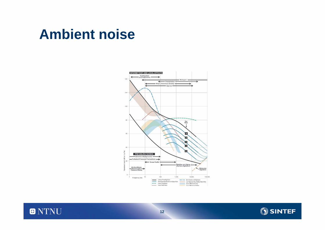
Ambient noise

13

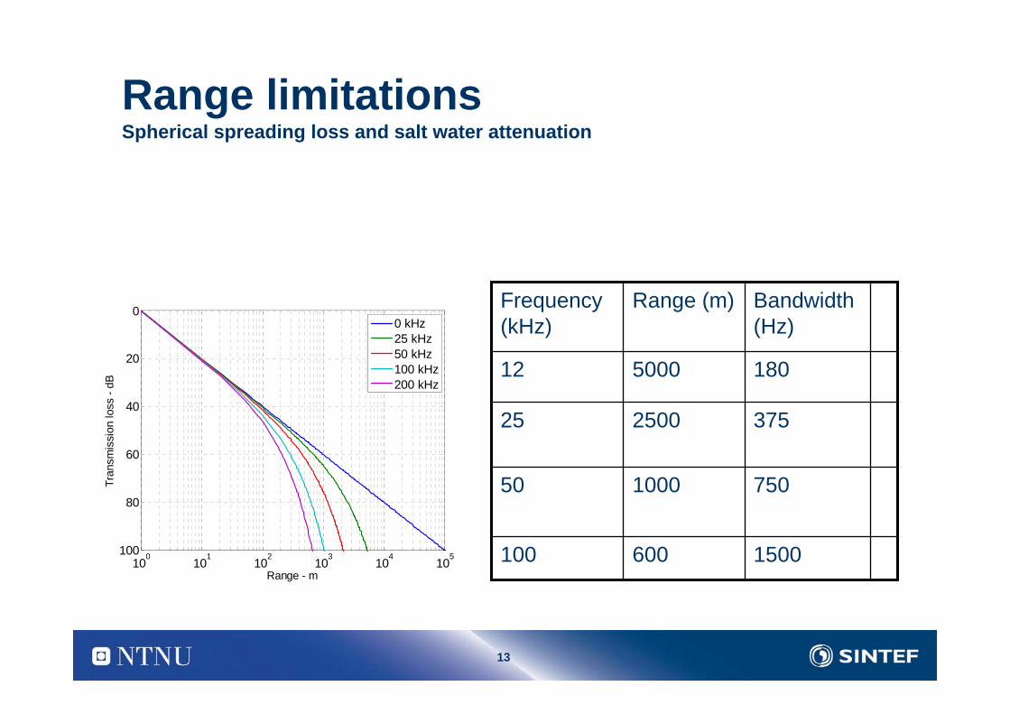
Range limitationsSpherical spreading loss and salt water attenuation

100

101

102

103

104

105

0

20

40

60

80

100

Range - m

Tran

smis

sion

loss

- dB

0 kHz25 kHz50 kHz100 kHz200 kHz

750100050

1500600100

375250025

180500012

Bandwidth (Hz)

Range (m)Frequency (kHz)

14

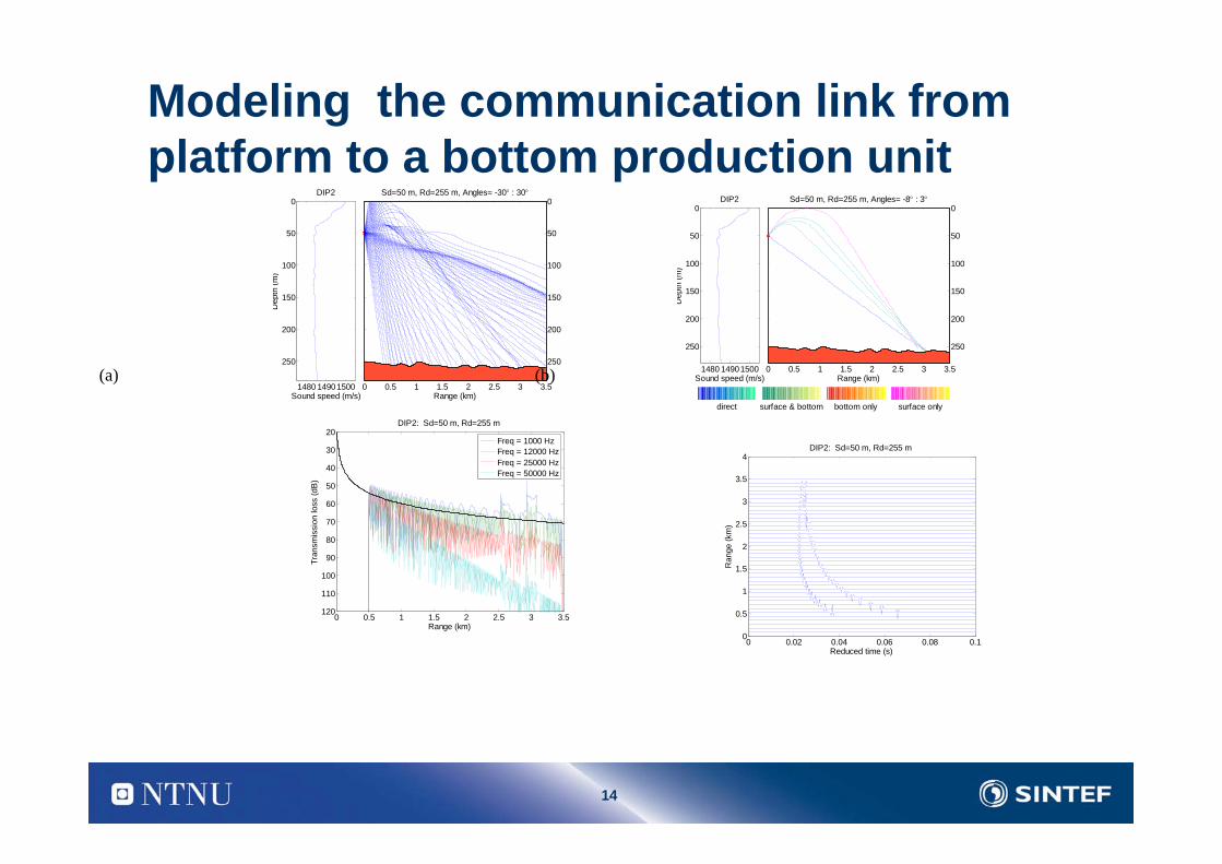
Modeling the communication link from platform to a bottom production unit

1480 14901500

0

50

100

150

200

250

Sound speed (m/s)

Dep

th (m

)

DIP2

0 0.5 1 1.5 2 2.5 3 3.5

0

50

100

150

200

250

Range (km)

Sd=50 m, Rd=255 m, Angles= -30° : 30°

1480 14901500

0

50

100

150

200

250

Sound speed (m/s)

Dep

th (m

)

DIP2

0 0.5 1 1.5 2 2.5 3 3.5

0

50

100

150

200

250

Range (km)

Sd=50 m, Rd=255 m, Angles= -8° : 3°

direct surface & bottom bottom only surface only

0 0.5 1 1.5 2 2.5 3 3.5

20

30

40

50

60

70

80

90

100

110

120

Range (km)

Tran

smis

sion

loss

(dB

)

DIP2: Sd=50 m, Rd=255 m

Freq = 1000 HzFreq = 12000 HzFreq = 25000 HzFreq = 50000 Hz

0 0.02 0.04 0.06 0.08 0.10

0.5

1

1.5

2

2.5

3

3.5

4

Reduced time (s)

Ran

ge (k

m)

DIP2: Sd=50 m, Rd=255 m

(a) (b)

15

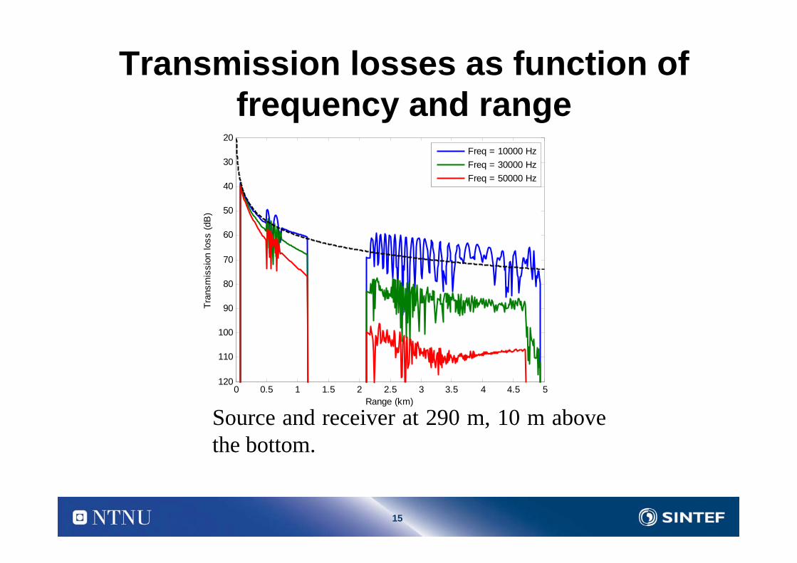
Transmission losses as function of frequency and range

Source and receiver at 290 m, 10 m above the bottom.

0 0.5 1 1.5 2 2.5 3 3.5 4 4.5 5

20

30

40

50

60

70

80

90

100

110

120

Range (km)

Tran

smis

sion

loss

(dB

)

Freq = 10000 HzFreq = 30000 HzFreq = 50000 Hz

16

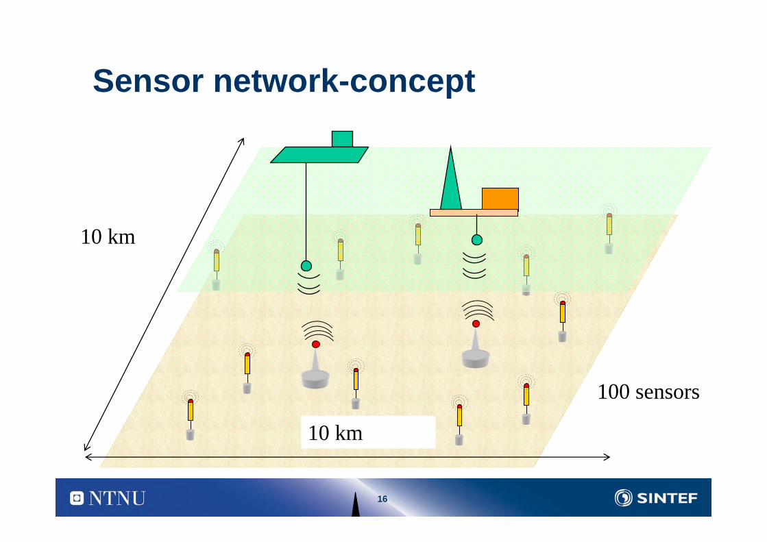
Sensor network-concept

10 km

10 km

100 sensors

17

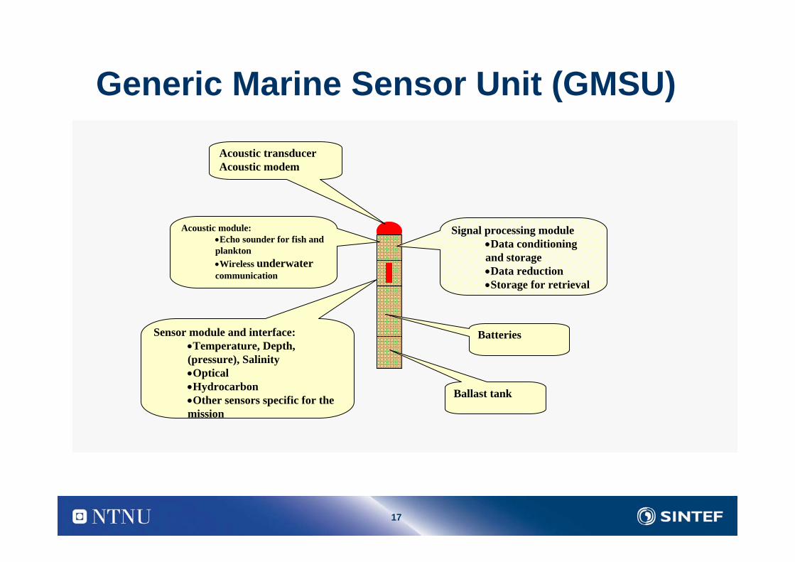
Generic Marine Sensor Unit (GMSU)

Signal processing module•Data conditioning and storage •Data reduction •Storage for retrieval

BatteriesSensor module and interface:•Temperature, Depth, (pressure), Salinity•Optical•Hydrocarbon•Other sensors specific for the mission

Ballast tank

Acoustic module:•Echo sounder for fish and plankton •Wireless underwatercommunication

Acoustic transducerAcoustic modem

18

Conclusion and recommendations

• We ( the underwater people) have a lot to learn from you(the earth people)

• If you want to be successful and useful in our field, youneed to understand our problem

19

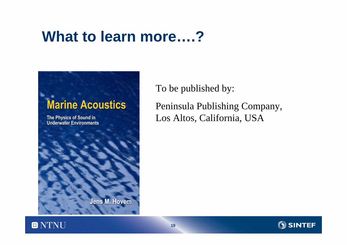
What to learn more….?

To be published by:

Peninsula Publishing Company, Los Altos, California, USA