Understanding the Shape of the Mixture Failure Rate (with ... · Understanding the Shape of the Mixture Failure Rate (with Engineering and Demographic Applications) Maxim Finkelstein

Understanding the Shape of the Mixture Failure Rate (with Engineering and Demographic Applications)

Maxim Finkelstein

Department of Mathematical Statistics, University of the Free State, 339 Bloemfon-tein 9300, South Africa.

e-mail : [email protected] and

Max Planck Institute for Demographic Research, Rostock, Germany

Abstract: Mixtures of distributions are usually effectively used for modeling hetero-geneity. It is well known that mixtures of DFR distributions are always DFR. On the other hand, mixtures of IFR distributions can decrease, at least in some intervals of time. As IFR distributions often model lifetimes governed by ageing processes, the operation of mixing can dramatically change the pattern of ageing. Therefore, the study of the shape of the observed (mixture) failure rate in a heterogeneous setting is important in many applications. We study discrete and continuous mixtures, obtain conditions for the mixture failure rate to tend to the failure rate of the strongest popu-lations and describe asymptotic behavior as ∞→t . Some demographic and engineer-ing examples are considered. The corresponding inverse problem is discussed. Keywords: failure (mortality) rate, mixture of distributions, aging distributions, mor-tality plateau, frailty 1. Introduction The wording of our title was inspired by the groundbreaking paper by Aalen and Gjessing (2001). These authors were discussing the shape of the ‘ordinary’ failure rate by using the stochastic processes-based reasoning. Our paper is devoted to the failure rate of mixtures and the employed methods are mostly based on the analysis of the corresponding lifetime distributions. Its genre is close to a review: in a compact way we are discussing and analyzing some of the relatively recent results in this area. This is not a ‘complete’ review of the subject as only those our findings and results of other authors are used that are aligned with our vision of this topic. We also include some new discussions, examples and specific results. Note that the paper by Steinsaltz and Wachter (2006) was also devoted to a qualitative analysis of the shape of the failure (mortality) rate for heterogeneous human populations at advanced ages. We deal with this application in Section 5.

One can hardly find homogeneous populations in real life, although most of the studies on failure rate modelling deal with a homogeneous case. Neglecting existing heterogeneity can lead to errors and misconceptions in stochastic analysis in reliabil-ity, survival and risk analysis as well as other disciplines.

Mixtures of distributions usually present an effective tool for modeling heterogene-ity. It is well known that mixtures of decreasing failure rate (DFR) distributions are always DFR (Barlow and Proschan, 1975). On the other hand, mixtures of increasing failure rate (IFR) distributions can decrease, at least in some intervals of time. Note that IFR distributions often used to model lifetimes governed by ageing processes, which means that the operation of mixing can dramatically change the pattern of population ageing, e.g., from positive ageing (IFR) to negative ageing (DFR). There-

2

fore, the study of the shape of the observed (mixture) failure rate in a heterogeneous setting is important in many applications (reliability, demography, risk analysis, etc).

A useful interpretation of mixing in heterogeneous populations is based on a notion of a non-negative, unobserved random parameter (frailty) Z . The term “frailty” was suggested in Vaupel et al. (1979) for the gamma-distributed Z . It is worth noting, however, that this specific case of the gamma-frailty model was, in fact, first consid-ered by the British actuary Robert Beard (Beard, 1959, 1971). Our presentation mostly deals with a study of the shape of the mixture failure rate in popular in applica-tions frailty models, i.e., additive, proportional and accelerated life models. A convincing ‘experiment’ showing the deceleration in the observed failure (mor-tality) rate is performed by nature. It is well known that human mortality follows the Gompertz lifetime distribution with an exponentially increasing mortality rate. It can be shown that the multiplicative gamma-frailty model results in this case in the mix-ture failure rate that asymptotically tends to a constant as ∞→t , although ‘individ-ual’ failure rates increase sharply as exponential functions for all 0≥t . This surpris-ing result can explain the recently observed human mortality plateau (Thatcher. 1999). Our presentation is partially based (but not limited) on chapters 6 and 7 of Finkel-stein (2008). As usually, we use the terms, “increasing” and “decreasing” meaning “non-decreasing” and “non-increasing”, respectively.

2. Failure Rate of Mixture of Two Distributions

Suppose, for instance, that a population of some manufactured items consists of items with and without manufacturing defects. The time to failure of an item picked up at random from this population can be obviously described in terms of mixtures. We start with a mixture of two lifetime distributions )(1 tF and )(2 tF with the pdfs )(1 tf and )(2 tf and failure rates )(1 tλ and )(2 tλ , respectively, whereas the Cdf, pdf and the failure rate of the mixture itself are denoted by )(tFm , )(tfm and )(tmλ , accord-ingly. This specific case will help us to analyze certain general patterns of the shape of the mixture failure rate for the case of continuous mixing distributions which is the main topic of this paper.

Let the masses π and π−1 define the discrete mixture distribution. The mixture survival function and the mixture pdf are

),()1()()( 21 tFtFtFm ππ −+=

),()1()()( 21 tftftfm ππ −+=

respectively. In accordance with the definition of the failure rate, the mixture failure rate in this case is

)()1()()()1()(

)(21

21

tFtFtftf

tm ππππλ

−+−+= .

As ,2,1),(/)()( == itFtft iiiλ this can be transformed into

)())(1()()()( 21 tttttm λπλπλ −+= , (2.1)

where the time-dependent probabilities are

3

)()1()()()1(

)(1,)()1()(

)()(

21

2

21

1

tFtFtF

ttFtF

tFt

ππππ

ππππ

−+−=−

−+= , (2.2)

It follows from Equation (2.1) that )(tmλ is contained between )}(),(min{ 21 tt λλ and )}(),(max{ 21 tt λλ . Specifically, if the failure rates are ordered as )()( 21 tt λλ ≤ , then

)()()( 21 ttt m λλλ ≤≤ . (2.3)

Differentiating (2.1) results in (Navarro and Hernandez, 2004):

22121 ))()()((1))(()())(1()()()( tttttttttm λλππλπλπλ −−−′−+′=′ . (2.4)

Assume that 2,1)( =itiλ are DFR. It follows from (2.3) that the mixture failure rate in this case is also decreasing, which is the well-known fact for general mixtures (Bar-low and Proschan, 1975).

As 2,1,1)0( == iFi , the initial value of the mixture failure rate ( 0=t ) is just the ‘ordinary’ mixture of initial values of the two failure rates, i.e.,

)0()1()0()0( 21 λππλλ −+=m .

When 0>t , the conditional probabilities )(tπ and )(1 tπ− are obviously not equal to π and π−1 , respectively. Assume that )()( 21 tt λλ ≤ . Dividing the numerator and denominator in the first equation in (2.2) by )(1 tF it is easy to see that the proportion of the survived up to t items in the mixed population, i.e., )(tπ is increasing ( )(1 tπ− is decreasing): the weakest items are dying out first. Therefore

0),()1()()( 21 >−+< ttttm λππλλ , (2.5)

Thus, )(tmλ is always smaller than the expectation )()1()( 21 tt λππλ −+ . Assume now that both )(1 tλ and )(2 tλ are increasing for 0≥t . Can the mixture failure rate initially (at, least, for small t ) decrease? Equation (2.4) helps us to give the positive answer to this question. The corresponding sufficient condition is

0))0()0()(1()()1()( 22121 <−−−′−+′ λλππλπλπ tt , (2.6)

where the derivatives are obtained at 0=t . Inequality (2.6), e.g, means that if

|)0()0(| 21 λλ − is sufficiently large, then the mixture failure rate is initially decreasing no matter how fast the failure rates )(1 tλ and )(2 tλ are increasing in the neighbour-hood of 0, which is a remarkable fact, indeed. Let, for instance,

2121222111 0,0,)(,)( aaccatctatct <<<<+=+= λλ ,

then if 2/1

21112 )1(

)1(���

����

�

−−+>−ππππ cc

aa ,

4

)(tmλ is initially decreasing. What about the asymptotic (for large t ) behaviour of )(tmλ ? Due to the weakest populations are dying first principle the intuitive guess would be: the mixture failure rate tends (in some suitable sense) to the failure rate of the strongest population as

∞→t . Block and Joe (1997) give some general conditions for this convergence. We will just consider here an important specific case of proportional failure rates that al-lows formulating these conditions explicitly:

)(),()( 111 tzztt λλλ =≡ , 12222 ),(),()( zztzztt >=≡ λλλ ,

where )(tλ is some baseline failure rate. We will distinguish between the conver-gence

0),()( 1 →− zttm λλ as ∞→t (2.7)

and the asymptotic equivalence

))1(1)(,()( 1 ozttm += λλ as ∞→t , (2.8)

which will mostly be used in the following alternative notation: ),(~)( 1zttm λλ as ∞→t .

When )(tλ has a finite limit as ∞→t , these relationships coincide. The following theorem (Finkelstein and Esaulova, 2001) specifies the corresponding conditions: Theorem 2.1. Consider the mixture model (2.1)-(2.2), where

0);(),(),(),( 122211 >>== zztzzttzzt λλλλ ,

and ∞→)(tλ as ∞→t . Then • Relationship (2.8) holds;

• Relationship (2.7) holds if

0})()(exp{)(0

12 →−− �t

duuzzt λλ as ∞→t . (2.9)

The proof is straightforward and is based on considering the quotient ),(/)( 1zttm λλ as in Block and Joe (1997).

Condition (2.9) is a rather weak one. In essence, it states that the pdf of a distribu-tion with an ultimately increasing failure rate tends to 0 as ∞→t . All distributions that are typically used in lifetime data analyses meet this requirement. Similar reasoning can be used for describing the shape of the failure rate for the mixture of 2>n distributions (Block and Joe, 1997; Finkelstein, 2008). We have described some approaches to describing the general pattern of the shape of the mixture failure rate for two distributions focusing on initial and tail behaviour. The concrete shapes can be versatile. We will just present here a few examples. More information on specific shapes of the mixture failure rate of two distributions can be found in Gurland and Sethuraman (1995), Jiang and Murhphy (1998), Gupta and Waren, (2001), Block, Li and Savits (2003), Block, Savits and Wondmagegnehu

5

(2003), Lai and Xie (2006), Navarro and Hernandez (2004), Wondmagegnehu (2004), Finkelstein (2008), Block et al (2008). Note that Vaupel and Yashin (1985) also ana-lyze different shapes of the mixture mortality rate for the relevant in demographic studies values of parameters.

• As follows from Gupta and Waren, (2001), the mixture of two gamma distributions with increasing failure rates (with the same scale parameter) can result either in the increasing mixture failure rate or in the modified bathtub (MBT) mixture failure rate (it first increases and then behaves like a bathtub (BT) failure rate). This shape agrees with our general reasoning of this section, as it can be easily verified that condition (2.6) does not hold in this case and therefore the initial decreasing is not possible.

• Similar shapes occur for the mixtures of two Weibull distributions with increas-ing failure rates. Note that that in this case, MBT shape results when p in Equation (2.1) is less than some 10, << ξξ and the mixture failure rate in-creases for ξ≥p (Jiang and Murhphy, 1998).

• Navarro and Hernandez (2004) state that the mixture failure rate of two trun-cated normal distributions (we are dealing with lifetime random variables), de-pending on parameters involved, can also be increasing, BT-shaped or MBT-shaped. The BT shape obtained via the generalized mixtures (when p is a real number and not necessarily ]1,0[∈p ) where studied in Navarro and Hernandez (2008).

• Block, Savits and Wondmagegnehu (2003) give explicit conditions which de-scribe the possible shapes of the mixture failure rate for two increasing linear failure rates. Again the possible shapes in this case are IFR, BT and MBT (for the non-crossing linear failure rates).

• Block et al (2008) present an interesting generalization when one of the distri-butions is itself a continuous mixture of exponentials (and therefore, decreas-ing) and the other is a gamma distribution. It is shown that for the specific val-ues of parameters involved the mixture failure rate has a BT shape. In essence, these authors are ‘constructing’ the BT shape using the specifically decreasing in ),0( ∞ to 00 >> λζ failure rate of the first distribution and the increasing to

0λ failure rate of the second distribution. Note that, as follows from (2.3), )(tmλ is contained between these two failure rates. Block et al (2008) also

prove that mixtures of DFR gamma distributions with an IFR gamma distribu-tion are bathtub and mixtures of modified Weibull distributions (the failure rate is decreasing not to 0 , as for ‘ordinary’ Weibull distribution, but to ζ ) with an IFR gamma are also bathtub.

It is worth noting that the analysis of the shape of the failure rate function (and the mixture failure rate as well) is often based on the Glaser’s approach (Glaser, 1980), which states that the shape of the failure rate is defined by the shape of the following function

)()(

)(tftf

t′

=η ,

6

which is usually easier to analyze than the shape of the corresponding failure rate )(/)()( tFtft =λ . For instance, when )(tη is increasing (decreasing) the failure rate

is also increasing (decreasing). However, our results mostly rely on some general properties of distributions and are more suitable, e.g., for asymptotic analysis. 3. Continuous Mixtures Let Z be a mixing random variable (frailty) with support in ),0[ ∞ and the pdf )(zπ . Similar to the previous section, the mixture survival function and the mixture pdf are defined as the following expectations:

,)(),()(

,)(),()(

0

0

�

�

=

=

t

m

t

m

dzzztftf

dzzztFtF

π

π (3.1)

respectively, where the notation for conditional functions ),()|( ztFzZtF == and ),()|( ztfzZtf == means that a lifetime distribution is indexed by parameter z .

The corresponding conditional failure rate is denoted by ),( ztλ , whereas the mixture (observed) failure rate is

�

�∞

∞

=

0

0

)(),(

)(),()(

dzzztF

dzzztftm

π

πλ . (3.2)

Equation (3.2) can be transformed to (Lynn and Singpurwalla, 1997):

�∞

=0

)|(),()( dztzzttm πλλ ,

�∞=

0

)(),(

),()()|(

dzzztF

ztFztz

π

ππ (3.3)

where )|( tzπ denotes the conditional pdf of Z on condition that tT > , i.e, an item described by a lifetime T with the Cdf )(tFm had survived in ],0[ t . Denote this ran-dom variable by tZ | . Obviously the masses )(tπ and )(1 tπ− in (2-1) correspond to

)|( tzπ in the continuous case. Under the mild assumptions (see Theorem 3.1), a similar to (2.5) property holds for the continuous case as well, i.e.,

0,)(),()()(0

>≡< �∞

tdzzzttt Pm πλλλ ; )()0( tPm λλ = (3.4)

meaning that the mixture failure rate is always smaller than the ‘ordinary’ expecta-tion. Thus, owing to conditioning, the mixture failure rate is smaller than the uncondi-tional one for each 0>t , which, as in the discrete case, can be interpreted via the weakest populations are dying out first principle. As time increases, those subpopula-tions that have larger failure rates have higher chances of dying, and therefore the proportion of subpopulations with a smaller failure rate increases.

7

The following theorem (Finkelstein and Esaulova, 2006) states also the condition for )()( tt mP λλ − to increase: Theorem 3.1. Let the failure rate ),( ztλ be differentiable with respect to both argu-ments and be ordered as

0],,[,,),,(),( 212121 ≥∈∀<< tbazzzzztzt λλ . (3.5)

Then

• Inequality (3.4) holds;

• If, additionally, zzt ∂∂ /),(λ is increasing in t , then )()( tt mP λλ − is increasing.

We will consider now two important in applications specific cases of model (3.3). Let ),( ztλ be indexed by parameter z in the following additive way:

ztzt += )(),( λλ , (3.6)

where )(tλ is a deterministic, continuous and positive function for 0>t . It can be viewed as some baseline failure rate. Equation (3.6) defines for ),0[ ∞∈z a family of ‘horizontally parallel’ functions. We will be interested in an increasing )(tλ . Apply-ing (3.3) to this model results in

]|[)()(),(

)(),()()(

0

0 tZEtdzztF

dzzztFzttm +=+=

�

�∞

∞

λθπ

πλλ , (3.7)

where, in accordance with (3.3), ]|[ tZE denotes the expectation of the random variable tZ | . It can be easily shown by direct derivation that

0)|(]|[' <−= tZVartZE . Differentiating (3.7) and using this proprty, we obtain the following result (Lynn and Singpurwalla,1997; Finkelstein and Esaulova, 2001).

Theorem 3.2. Let )(tλ be an increasing, convex function in ),0[ ∞ . Assume that )|( tZVar is decreasing in t ),0[ ∞∈ and

)0()0|( λ′>ZVar .

Then )(tmλ decreases in ),0[ c and increases in ),[ ∞c , where c can be uniquely defined from the following equation:

)()|( ttZVar λ′= .

It follows from this theorem that the corresponding model of mixing results in the bathtub shape of the mixture failure rate: it first decreases and then increases, con-verging to the failure rate of the strongest population, which is )(tλ in our case. It seems that the conditional variance )|( tZVar should decrease, as the “weak popula-tions are dying out first” when t increases. It turns out, however, that this intuitive reasoning is not true for the general case and some specific distributions can result in

8

initially increasing )|( tZVar . The corresponding counter-example can be found in Finkelstein and Esaulova (2001). It is also shown that )|( tZVar is always decreasing in ),0[ ∞ when Z is gamma-distributed. The most popular and elaborated in applications model of mixing is the multiplica-tive one:

)(),( tzzt λλ = , (3.8)

where, as previously, the baseline )(tλ is a deterministic, continuous and positive function for 0>t . In survival analysis, (3.8) is usually called a multiplicative frailty model (proportional hazards). The mixture failure rate in this case is

]|[)()|(),()(0

tZEtdztzzttm λπλλ == �∞

. (3.9)

Differentiating both sides gives

]|[)(]|[)()( tZEttZEttm ′+′=′ λλλ . (3.10)

Thus, when 0)0( =λ , the failure rate )(tmλ increases in the neighbourhood of 0=t . Further behaviour of this function depends on the other parameters involved. Similar to the additive case, =′ ]|[ tZE 0)|()( <− tZVartλ , which means that ]|[ tZE is de-creasing in t (Gupta and Gupta, 1996). Therefore, it follows from Equation (3.9) that the function )(/)( ttm λλ is a decreasing one, which imply that )(tλ and )(tmλ cross at most at only one point. It immediately follows from Equation (3.10) that when )(tλ is decreasing, )(tmλ is also decreasing (another proof of this well-known property). When 0)0( ≠λ and

][)(

)0()0(

2 ZEZVar≤

′λλ

,

the mixture failure rate is decreasing in 0),,0[ >εε meaning, e.g., that for the fixed ][ZE the variance of Z should be sufficiently large.

Asymptotic behavior of )(tmλ as ∞→t for this and other (more general models will be discussed in Section 6. Note that the accelerated life model (ALM) to be stud-ied in this section does not allow the foregoing reasoning based on considering expec-tation ]|[ tZE . 4. Some Examples

4.1 Weibull and Gompertz distributions

Consider multiplicative frailty model (3.8). Let Z be a gamma-distributed random variable with shape parameter α and scale parameter β and let 1,)( 1 >= − γγλ γtt be the increasing failure rate of the Weibull distribution, ∞=∞→ )(lim tt λ . The mixture failure rate )(tmλ in this case, can be obtained by the direct integration, as in Finkel-stein (2008) (see also Gupta and Gupta, 1996):

γ

γ

βαβγλ

tt

tm +=

−

1)(

1

. (4.1)

9

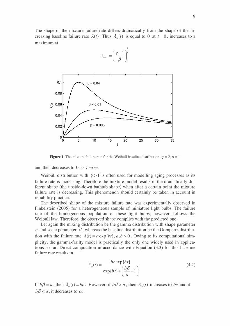
The shape of the mixture failure rate differs dramatically from the shape of the in-creasing baseline failure rate )(tλ . Thus )(tmλ is equal to 0 at 0=t , increases to a maximum at

γ

βγ

1

max1���

����

� −=t

Figure 1. The mixture failure rate for the Weibull baseline distribution, 1,2 == αγ

and then decreases to 0 as ∞→t .

Weibull distribution with 1>γ is often used for modelling aging processes as its failure rate is increasing. Therefore the mixture model results in the dramatically dif-ferent shape (the upside-down bathtub shape) when after a certain point the mixture failure rate is decreasing. This phenomenon should certainly be taken in account in reliability practice. The described shape of the mixture failure rate was experimentally observed in Finkelstein (2005) for a heterogeneous sample of miniature light bulbs. The failure rate of the homogeneous population of these light bulbs, however, follows the Weibull law. Therefore, the observed shape complies with the predicted one. Let again the mixing distribution be the gamma distribution with shape parameter c and scale parameter β , whereas the baseline distribution be the Gompertz distribu-tion with the failure rate 0,},exp{)( >= babtatλ . Owing to its computational sim-plicity, the gamma-frailty model is practically the only one widely used in applica-tions so far. Direct computation in accordance with Equation (3.3) for this baseline failure rate results in

.1}exp{

}exp{)(

��

���

� −+=

ab

tb

tbbctm β

λ (4.2)

If ab =β , then bctm ≡)(λ . However, if ab >β , then )(tmλ increases to bc and if ab <β , it decreases to bc .

0 5 10 15 20 25 30 350

0.02

0.04

0.06

0.08

0.1

t

λ(t)

β = 0.04

β = 0.01

β = 0.005

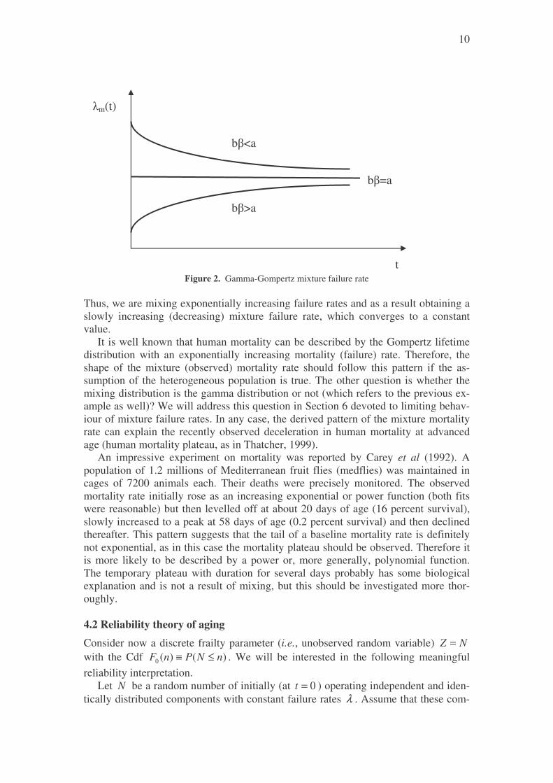
10

Figure 2. Gamma-Gompertz mixture failure rate Thus, we are mixing exponentially increasing failure rates and as a result obtaining a slowly increasing (decreasing) mixture failure rate, which converges to a constant value. It is well known that human mortality can be described by the Gompertz lifetime distribution with an exponentially increasing mortality (failure) rate. Therefore, the shape of the mixture (observed) mortality rate should follow this pattern if the as-sumption of the heterogeneous population is true. The other question is whether the mixing distribution is the gamma distribution or not (which refers to the previous ex-ample as well)? We will address this question in Section 6 devoted to limiting behav-iour of mixture failure rates. In any case, the derived pattern of the mixture mortality rate can explain the recently observed deceleration in human mortality at advanced age (human mortality plateau, as in Thatcher, 1999). An impressive experiment on mortality was reported by Carey et al (1992). A population of 1.2 millions of Mediterranean fruit flies (medflies) was maintained in cages of 7200 animals each. Their deaths were precisely monitored. The observed mortality rate initially rose as an increasing exponential or power function (both fits were reasonable) but then levelled off at about 20 days of age (16 percent survival), slowly increased to a peak at 58 days of age (0.2 percent survival) and then declined thereafter. This pattern suggests that the tail of a baseline mortality rate is definitely not exponential, as in this case the mortality plateau should be observed. Therefore it is more likely to be described by a power or, more generally, polynomial function. The temporary plateau with duration for several days probably has some biological explanation and is not a result of mixing, but this should be investigated more thor-oughly. 4.2 Reliability theory of aging

Consider now a discrete frailty parameter (i.e., unobserved random variable) NZ = with the Cdf )()(0 nNPnF ≤≡ . We will be interested in the following meaningful reliability interpretation. Let N be a random number of initially (at 0=t ) operating independent and iden-tically distributed components with constant failure rates λ . Assume that these com-

b�<a

b�>a

t

�m(t)

b�=a

11

ponents form a parallel system, which, according to Gavrilov and Gavrilova (2001), models the lifetime of an organism on some suitable level (generalization to the se-ries-parallel structure is straightforward). These authors also provide a biological jus-tification of the model. In each realization 1, ≥= nnN , the degradation process of pure death can be defined as just the number of failed components. When this number reaches n , the death of an organism occurs. Denote by )(tnλ the mortality (failure) rate, which describes nT –the time to death for the fixed ,...2,1, == nnN ( 0=n is excluded, as there should be at least one operating component at 0=t ). It is shown in Gavrilov and Gavrilova (2001) that as 0→t , this mortality rate tends to an increas-ing power function (the Weibull law), which is a remarkable fact. On the other hand, for random N , similar to (2.1) and (3.3), the observed (mixture) mortality rate is given as the following conditional expectation with respect to N :

]|)([)( tTtEt Nm >= λλ . (4.3)

Therefore, as previously, )(tmλ is a conditional expectation (on condition that the sys-tem is operable at t ) of a random mortality rate )(tNλ . Note that, for small t , this operation can approximately result in the unconditional expectation

)()]([)(1

tPtEt nn

nNm λλλ �∞

=

=≈ , (4.4)

where ]Pr[ nNPn =≡ , but the limiting transition, as 0→t , should be performed carefully in this case. As ∞→t , we observe the following mortality plateau (Finkel-stein and Vaupel, 2006):

λλ →)(tm . (4.5)

This is due to the fact that the conditional probability that only one component with the failure rate λ is operating tends to 1 as ∞→t (on condition that the system is operating).

Assume now that N is Poisson distributed with parameter η (on condition that the system is operable at 0=t ). Therefore

,...2,1,})exp{1(!

}exp{ =−−

−= nn

Pn

n ηηη

.

It can be shown via direct integration that the time to death in our simplified model has the following Cdf (Steinsaltz and Evans, 2004):

.}exp{1

}}exp{exp{1]Pr[)(

ηλη

−−−−−=≤= t

tTtF (4.6)

The corresponding mixture mortality rate is

1}}exp{exp{}exp{

)(1)(

)(−−

−=−

′=

tt

tFtF

tm ληληλλ . (4.7)

Performing, as ∞→t , the limiting transition in (4.7), we also arrive at the mortality plateau (4.5).

12

In fact, the mortality rate given by Equation (4.7) is far from the exponentially in-creasing Gompertz law. The Gompertz law can erroneously follow (as in Gavrilov and Gavrilova (2001)) from (4.4) if this approximation is used formally, without con-sidering a proper conditioning in (4.3), However, for some specific values of parame-ters and sufficiently small t , exponential approximation can still hold. The relevant discussion can be found in Steinsaltz and Evans (2004). 4.3 Burn-in and minimal repair in heterogeneous populations

In this example, we want to clarify the notion of minimal repair for heterogeneous case. Minimal repair is usually defined in a classical sense as the repair that brings an item to the statistically identical state it had just prior to the failure (Barlow and Pro-schan, 1975). For an item with the distribution function )(tF , that has failed and was instantaneously minimally repaired at time at = , it means that the time to the next failure is distributed as ))(1/())()(( aFtFatF −−+ , which is equal to the distribution of the corresponding remaining lifetime of a nonrepairable item. This type of minimal repair is sometimes called a statistical minimal repair. (Arjas and Norros, 1989; Finkelstein, 1992) to emphasize the repair to the mentioned above statistically identi-cal state, but usually the term “statistical” is omitted. For a repairable item with a de-creasing failure rate, minimal repairs during burn-in result in an improvement in reli-ability for further field usage. A similar conclusion can be obtained for the case of a bathtub failure rate. In this case, the burn-in procedure should be performed in the time interval where the failure rate is decreasing. It is not so simple to define minimal repair for heterogeneous populations (Finkel-stein, 2004). Assume that our population consists of the weak and strong subpopula-tions with the distributions functions )(tFS and )(tFW , respectively, and therefore, the lifetime of a picked at random item is described by a mixture of two distributions as in Section 2, i.e., )()1()()( tFtFtF WSm ππ −+= . This means that formally, in accordance with the classical definition of minimal repair, the time to the next failure should be distributed as ))(1/())()(( aFtFatF mmm −−+ . The only theoretical possibility to per-form this operation is to replace the failed item by another item from our population that had functioned the same time but did not fail. It is also obvious that it is impossi-ble in practice to perform this ideal statistical minimal repair for our heterogeneous setting. As discussed in Section 2, the failure rates of mixtures of two distributions are often decreasing (at least initially) and therefore, the same burn-in considerations as in the homogeneous case can be applied, but we note once again that minimal repair of this kind usually cannot be realized in practice. On the other hand, we can execute another type of minimal repair. Assume that the corresponding minimal repair is, in fact, a physical minimal repair (Finkelstein, 1992) in the sense that a ‘physical operation’ of repair (not a replacement as above) brings an item in the state which is ‘statistically identical’ to the state it had just prior the failure. Note that, obviously, we do not know whether the failed item is ‘strong’ or ‘weak’. On the other hand, the described operation of repair in some sense retains this property automatically: if an item is, e.g., ‘strong’, the time to the next failure is distributed as ))(1/())()(( aFtFatF sSS −−+ . An example of this ‘physical operation’ is when a ‘small’ defect (fault) is corrected (repaired) upon failure, whereas a number of the possible inherent defects in the item is ‘large’. In practice, the physical minimal repair of the described type can be usually performed (at least approximately) and therefore our assumption is quite realistic. It is also clear that for

13

the homogeneous case these two types of minimal repair (approximately) coincide, i.e., result in the same distribution of time to the next failure, whereas they differ for the mixed population. Not that the burn-in process for repairable items for the de-scribed case is, in fact, a test procedure which helps to classify an item from a mixed population as being ‘strong’ or ‘weak’. 4.4. Parondox paradox

There are many situations where the concept of mixing helps to explain results that seem to be paradoxical. A meaningful example is a Parondo paradox in game theory (Harmer and Abbot, 1999), which describes the dependent losing strategies which eventually win. Di Crescenzo (2007) presents the reliability interpretation of this paradox. This author compares pairs of systems with two independent components in each series. The i th component of the first system ( 2,1=i ) is less reliable than the corresponding component of the second one (in the sense of the usual stochastic or-der). The first system is modified by a random choice of its components. Each com-ponent is chosen randomly from a set of components identical to the previous ones, and the corresponding distribution of a new component is defined as a discrete mix-ture (with 2/1=π ) of initial distributions of components of the first system. Thus, the described randomization defines a new system that is shown to be more reliable (under suitable conditions) than the second one, although initial components are less reliable than those of the second system. A formal proof of this phenomenon is pre-sented in this paper, but the result can easily be interpreted in terms of the decreasing failure rate of the corresponding mixture. 4.5. Coherent systems

In a rather unexpected way mixtures can also be used to represent lifetimes of coher-ent systems. It turns out (Samaniego, 2007) that the lifetime distribution of a coherent system of n i.i.d. components )(tF (with common Cdf )(tFc ) can be written as a function that depends on the system’s design only through signatures in the following ‘mixture form”:

)Pr()( :1

tXstF ni

n

ii >=�

=

, (4.8)

where )Pr()( tTtF >= nnnn XXX ::2:1 ,..., are order statistics obtained from n lifetimes

of components, )Pr( :nii XTs == and the vector ( nsss ,...,, 21 ) is called the system’s signature. Kochar et al (1999) consider relationships between different stochastic orders for signatures of two systems and their lifetimes. The shape of the system’s failure rate can be also analyzed using (4.8) and our reasoning of the previous sections (at least, for some simple examples). Section 5. Mixture Failure Rate for Large t Among the first to consider the limiting behaviour of mixture failure rates for the con-tinuous mixtures were Clarotti and Spizzichino (1990). They showed that the mixture failure rate for a family of exponential distributions with parameter ),[ ∞∈ aα con-verges to the failure rate of the strongest population, which is a in this case. Block et al (1993), Block, Li and Savits (2003) and Li (2005) extended this to a general case.

14

As the approach (and obtained important mathematical results) of these authors is very general and some assumptions are rather restrictive, it does not provide specific asymptotic relationship that can be used in practical analysis for mixed populations. In order to be able to perform this analysis, Finkelstein and Esaulova (2006) devel-oped an approach that was applied to reasonably general survival model that allows for explicit asymptotic relationships and covers (as specific cases) three most popular in survival analysis frailty models: additive, proportional and accelerated life. The main results that were obtained using this approach are discussed below. Let 0≥T be a lifetime with the cdf )(tF , pdf )(tf and the failure rate )(tλ . Let, as previously, these functions be indexed by the realization of the frailty parameter

zZ = , i.e., ),(),,(),,( ztztfztF λ , respectively. Consider the following general sur-vival model:

),())((),( ttzAzt ψφ +=Λ (5.1)

where �≡Λt

ztzt0

),(),( λ denotes the corresponding cumulative failure rate and

)(⋅A , )(⋅ψ and )(⋅φ are some increasing, differentiable functions of their arguments. The meaning of relationship (5.1): we perform a scale transformation )(tφ in the ar-gument of the cumulated failure rate )(tΛ and ‘insert’ a frailty parameter. An impor-tant feature of the model is that parameter z is a multiplier. This model includes a number of well-known in survival analysis and reliability specific cases, i.e., Additive Model: Let

,)(,)( ttuuA =≡ φ 0)0( =ψ . Then

)(),(),(),( tztzttzzt ψψλ +=Λ′+= (5.2)

PH (multiplicative) Model: Let

)()(,)( ttuuA Λ=≡ φ .

Then

�=Λ=Λ

=t

duuztzzt

tzzt

0

)()(),(

),(),(

λ

λλ (5.3)

Accelerated Life Model: Let

ttuuA =Λ≡ )(),()( φ .

Then

� Λ==Λzt

ztduuzt0

),()(),( λ (5.4)

)(),( ztzzt λλ = (5.5)

15

We are interested in asymptotic behaviour (as )∞→t of )(tmλ . For simplicity of notation (and, in fact, not loosing the generality), we will assume further that

0)( =tψ . Theorem 5.1. Let the cumulative failure rate ),( ztΛ be given by Equation (5.1) ( 0)( =tψ ) and let the mixing pdf ),0[),( ∞∈zzπ be defined as

)()( 1 zzz ππ α= , (5.6)

where 1−>α and 0)0(),( 11 ≠ππ z is a function bounded in ),0[ ∞ and continuous at 0=z . Assume also that ∞→)(tφ as ∞→t and that )(sA satisfies

�∞

∞<−0

)}(exp{ dsssA α . (5.7)

Then

)()(

)1(~)(tt

tm φφαλ ′

+ , (5.8)

where, as usual, asymptotic notation )(~)( tbta as ∞→t means that 1)(/)(lim =→∞ tbtat . As we had mentioned, another possible notation for (5.8) is

))1(1)((/)()1()( otttm +′+= φφαλ .

The proof of this result is cumbersome and is based on Abelian-type theorems for the corresponding asymptotic integrals. That is why the multiplicative form in

))(( tzA φ is so important. The specific case of this theorem for the multiplicative model (5.5) was independently considered by Steinsaltz and Wachter (2006). Assumption (5.6) just states the ‘form’ of the admissible mixing distribution and holds for the main lifetime distributions, such as Weibull, gamma, truncated normal, etc. However it does not hold for a lognormal distribution, as the corresponding as-ymptote is proportional to z/1 when 0→z . Assumption (5.7) is a very weak one (weaker than just having a finite expectation for a lifetime) and can be omitted in practical analysis.

A crucial feature of this result is that the asymptotic behaviour of the mixture fail-ure rate depends only on the behaviour of the mixing distribution in the neighbour-hood of 0 and on the derivative of the logarithm of the scale function )(tφ , i.e.,

)(/)())((log ttt φφφ ′=′ .

When 0)0( ≠π and )(zπ is bounded in ),0[ ∞ , the result does not depend on the mix-ing distribution at all , as 0=α in this case. Intuitively, the qualitative meaning is quite clear: as ∞→t , only the most robust survivors are left and in, accordance with the model (5.1), this corresponds to the small values of z (weak populations are dy-ing out first). It is easy to see that for the multiplicative model (5.3), equation (5.8) reduces to

16

�

+tm

duu

tt

0

)(

)()1(~)(

λ

λαλ . (5.9)

and to

ttm

1~)(

+αλ (5.10)

for the ALM (5.4)-(5.5). Note that (5.10) is a really surprising result, as the shape of the mixture failure rate for large t does not depend on the baseline distribution )(tF . It is also dramatically different from the multiplicative case (5.9). This means that the ‘nature’ of the ALM is such that it ignores’ the baseline distribution for large t . Comparing (5.9) and (5.10) we see that the latter will never result in the asymp-totically flat observed failure rate (mortality plateau), whereas the multiplicative model can as in the case of a gamma frailty model for the Gompertz distribution (see Equation 4.2 and discussion in the next section). Note that, by direct integration, Equation (4.2) can be generalized to the case of an arbitrary (absolutely continuous) baseline distribution characterized by the failure rate

)(tλ :

�+=

Λ+= tm

duu

tct

tct

0

)(

)()(

)()(

λβ

λβ

λλ . (5.11)

It is clear that 1+= αc for the gamma pdf and this formula perfectly comply with the general asymptotic result (5.9) and a classical result by Vaupel et al (1979). Let, for instance, )(zπ be the uniform density in ]1,0[ and let also

}exp{)( tt =λ ( 1, =ba for simplicity of notation). Then }exp{),( tzzt =λ and

})exp{1(1

)(),(0

ωω

π −−=�∞

dzzztF ,

�∞

=0

)(),( dzzztf π

��

� −−+−−+ })exp{1(1}exp{

)1( 2 ωωω

ωω

where 1}exp{ −= tω and ∞→ω as ∞→t . Therefore, in accordance with Equation (3.2):

1)(lim =∞→ tmt λ . The same limit holds for )(tmλ in (5.11) for the considered specific values of parame-ters. This example illustrates the fact that the asymptotic value of the mixture failure rate does not depend on a mixing distribution if 0)0( ≠π .

Theorem 5.1 deals with the case when the support of a mixing distribution includes 0 , i.e., ),0[ ∞∈z . In this case, the strongest population cannot usually be properly defined. If, however, the support is separated from 0 , the mixture failure rate can tend to the failure rate of the strongest population as ∞→t . The following theorem (Finkelstein and Esaulova, 2006) states reasonable conditions for this convergence (we assume, for simplicity, as previously, that 0)( =tψ ):

17

Theorem 5.2. Let, as in Theorem 5.1, the class of lifetime distributions be defined by Equation (5.1), where ∞→)(tφ , 0)( =tψ and let )(sA be twice differentiable.

Assume that, as ∞→s

0))(()(

2 →′′′sAsA

(5.12)

and

∞→′ )(sAs . (5.13)

Also assume that for all cbacb <> ,, , the quotient )(/)( csAbsA ′′ is bounded as ∞→s . Finally, let the mixing pdf )(zπ be defined in 0),,[ >∞ aa , bounded in this

interval and continuous at az = and 0)( ≠aπ . Then

)).(()(~)( taAtatm φφλ ′′ (5.14)

The assumptions of this theorem are rather natural and hold at least for the specific models under consideration and for the main lifetime distributions. Assume addition-ally that the family of failure rates ),( ztλ is ordered in z (as for additive or multipli-cative models), i.e.,

,0],,[,,),,(),( 212121 >∞∈∀<< aazzzzztzt λλ . (5.15)

The right-hand side of (5.14) can be interpreted in this case as the failure rate of the strongest population. Specifically, for the multiplicative model:

)(~)( tatm λλ . (5.16)

Thus, as intuition suggests, the mixture failure rate asymptotically does not depend on a mixing distribution. A similar result holds also for the case when there is a singular-ity in the pdf of the mixing distribution of the form:

)()()( 1 azazz −−= ππ α , (5.17)

where 1−>α and )(1 az −π is bounded, 0)0(1 ≠π . 6. Mortality plateaus As it was mentioned in Section 1, demographers had recently observed the decelera-tion in human mortality at advanced ages which eventually results in human mortality plateau (Thatcher, 1999). The most reasonable explanation of this fact is via the con-cept of heterogeneity of human population which obviously takes place. The follow-ing refers to the interpretation of our results for this application.

• As follows from Equation (5.9), the ALM (5.5) never results in the asymptoti-cally flat failure rate. Moreover, it asymptotically tends to 0 and does not de-pend on a baseline distribution, which is Gompertz for the case under consid-eration

18

• The only function )(tg , for which �t

o

duugtg )(/)( tends to a constant as ∞→t ,

is the exponential function. Therefore, as follows from relationship (5.9), the asymptotically flat rate in the multiplicative model (5.3) can result via mixing a random lifetime distributed only in accordance with the Gompertz distribution or in accordance with a distribution with the failure rate that asymptotically converges to an exponential function.

• In accordance with Theorem 5.1, the admissible mixing distributions (i.e., the

distributions that can lead to the asymptotically flat mortality rate) are those with behaviour as 1, −>ααz for 0→z . The behaviour outside the neighbour-hood of 0 does not contribute to asymptotic properties of the failure rate. Therefore, the power law (Weibull distribution), the gamma distribution and some other distributions are admissible. Note that, when the mixing pdf is such that 0)0( ≠π and has a finite limit when 0→z (as, e.g., for the exponential distribution), relationship (5.9) reduces to

�tm

duu

tt

0

)(

)(~)(

λ

λλ

and therefore, the mixture mortality rate does not depend on the mixing distribution at all! The same result holds for, e.g., the mixing density that is

0,/1 >aa in ],0[ a and is 0 in ),( ∞a (uniform distribution).

In view of the foregoing discussion, the asymptotically flat rate (as for human populations) can be viewed as an indication of: - that the mixing model is multiplicative,

- that the underlying distribution is definitely Gompertz or asymptotically con-verges to the Gompertz distribution,

- that the mixing pdf is proportional to 1, −>zzα , when 0→z , e.g., the gamma distribution. The form of this distribution outside neighbourhood of 0 has no influence on the asymptotic behaviour ( ∞→t ) of )(tλ .

7. Inverse Problem A well-known fact from survival analysis states that the failure data alone do not uniquely define a mixing distribution and additional information (e.g., on covariates) should be taken into account (a problem of non-identifiability, as, e.g., in Tsiatis, 1974 and Yashin and Manton, 1997). On the other hand, the following inverse prob-lem can be solved analytically at least for additive and multiplicative models of mix-ing (Esaulova, 2006; Finkelstein, 2008): Given the mixture failure rate )(tmλ and the mixing pdf )(zπ , obtain the failure rate

)(tλ of the baseline distribution.

19

This means that under certain assumptions any shape of the mixture failure rate can be constructed by the proper choice of the baseline failure rate. To illustrate this state-ment, consider the additive model (3.6):

})(exp{))((),(},)(exp{),( zttztztfzttztF −Λ−+=−Λ−= λ . (7.1)

Therefore, the mixture survival function in (3.1) can be written via the Laplace trans-form as

)()}(exp{)(}exp{)(exp{)( *

0

ttdzzztttFm ππ Λ−=−Λ−= �∞

, (7.2)

where, }][exp{)(* ztEt −=π is the Laplace transform of the mixing pdf )(zπ . There-fore, Equation (3.7) yields

)(log)()(}exp{

)(}exp{)()( *

0

0 tdtd

tdzzzt

dzzztzttm πλ

π

πλλ −=

−

−+=

�

�∞

∞

(7.3)

and the solution of the inverse problem for this special case is given by the following relationship:

]|[)()(log)()( * tZEttdtd

tt mm −=+= λπλλ . (7.4)

If the Laplace transform of the mixing distribution can be derived explicitly, then Equation (7.4) gives a simple analytical solution for the inverse problem. Assume, e.g., that ‘we want’ the mixture failure rate to be constant, i.e., ctm =)(λ . Then the baseline failure rate is obtained as

]|[)( tZEct −=λ .

The corresponding survival function for the multiplicative model (3.8) is )}(exp{ tzΛ− and the mixture survival function for this specific case is

�∞

Λ=Λ−=0

* ))(()()}(exp{)( tdzztztFm ππ . (7.5)

It is obtained in terms of the Laplace transform of the mixing distribution as a func-tion of the cumulative baseline failure rate )(tΛ . Therefore

))((log)( * tdtd

tm Λ−= πλ . (7.6)

The general solution to the inverse problem in terms of the Laplace transform is also simple in this case. Note that

)}(exp{))((* tt mΛ−=Λπ , (6.7)

where )(tmΛ denotes the cumulative mixture failure rate. Applying the inverse

Laplace transform )(1 ⋅−L to both sides of this equation finally results in

20

)})((exp{)()( 1 tLdtd

tt mΛ−=Λ′= −λ . (7.8)

The Laplace transform methodology in multiplicative and additive models is usu-ally very effective. It constitutes a convenient tool for dealing with mixture failure rates when the Laplace transform of the mixing distribution can be obtained explic-itly. The exponential family (Hougaard, 2000) presents a wide class of such distribu-tions. The corresponding pdf is defined in this case as

)()(}exp{

)(θη

θπ zgzz

−= , (7.9)

where )(zg and )(zη are some positive functions and θ is a parameter. The function )(θη plays the role of a normalizing constant ensuring that the pdf integrates to 1.

The gamma, the inverse Gaussian and the stable distributions are relevant examples. Note that the Laplace transform of )(zπ depends only on the normalizing function

)(zη (Hougaard, 2000), i.e.,

�∞ +=−≡0

*

)()(

)(}exp{)(θη

θηππ sdzzszs

This means that under certain assumptions any shape of the mixture failure rate can be constructed by the proper choice of the baseline failure rate. Specifically, for the ex-ponential family of mixing densities and for the multiplicative model under considera-tion, the mixture failure rate is obtained as

)(

))((log)(

θηθηλ t

dtd

tm

Λ+−=

))((

))(())(()(

t

ttd

d

tΛ+

Λ+Λ+−=

θη

θηθλ . (7.10)

Therefore, the solution to the inverse problem can be obtained in this case as the de-rivative of the following function:

θθηλη −−=Λ − ))()}((exp{)( 1 tt m . (7.11)

It can be easily calculated (Finkelstein, 2008) that when the mixing pdf is gamma with parameters α and β , the solution of the inverse problem is obtained as

���

���Λ=

αλ

αβλ )(

exp)()(t

tt mm . (7.12)

Assume that the mixture failure rate is constant, i.e., ctm =)(λ . It follows from (7.12) that for obtaining a constant )(tmλ the baseline )(tλ should be exponentially increas-ing, i.e.,

21

���

���=

ααβλ )

exp)(ct

ct .

But this is what we would really expect. As we already mentioned, this result is really surprising: we are mixing the exponentially increasing family of failure rates and ar-riving at a constant mixture failure rate. 8. Concluding Remarks

The mixture failure rate )(tmλ in frailty models is a conditional expectation of a ran-dom failure rate ),( Ztλ . A family of failure rates of subpopulations

∞≤<≤∈ babazzt 0],,[),,(λ describes heterogeneity of a population itself. One can hardly find homogeneous populations in real life, although most studies on failure rate modelling deal with a homogeneous case. Neglecting existing heterogeneity can lead to substantial errors and misconceptions in stochastic analysis in reliability, survival and risk analysis and other disciplines. If, for instance, a replacement is scheduled for an item from a heterogeneous population with exponentially distributed subpopula-tions, then the necessity of this replacement should be questioned, as the observed failure (mixture) failure rate is decreasing. Therefore, it may happen in this case that the failure rate of the replacement item can be larger than the failure rate of the used one.

Mixtures of increasing failure rate distributions can decrease at least in some inter-vals of time, which means that the IFR class of distributions is not closed under the operation of mixing. As IFR distributions usually model lifetimes governed by ageing processes, the operation of mixing can dramatically change the pattern of ageing, e.g., from positive ageing (IFR) to negative ageing (DFR).

The mixture failure rate is ‘bent down’ due to “the weakest populations are dying out first” effect. This should be taken into account when analysing the failure data for heterogeneous populations.

There are many applications where the behaviour of the failure rate at relatively large values of t is really important. The relevant example is the oldest-old mortality of humans when the exponentially increasing Gompertz mortality curve is ‘bent down’ at advanced ages (mortality plateau). The other example deals with a mixture of subpopulations with increasing (Weibull) subpopulations. In this case the mixture failure rate tends to 0 as ∞→t .

Some of the obtained results are really surprising. For example, when the support of the mixing distribution is ),0[ ∞ , the mixture failure rate in the accelerated life model converges to 0 as ∞→t and does not depend on the baseline distribution. Under reasonable assumptions, we show also that the asymptotic behaviour of the mixture failure rate for other models under consideration depends only on the behav-iour of the mixing distribution in the neighbourhood of the left-hand endpoint of its support, and not on the whole mixing distribution. References

1. Arjas, E., and Norros, I. (1989). Change of life distribution via a hazard transforma-tion: an inequality with application to minimal repair. Mathematics of Operations Re-search, 14, 355-361.

22

2. Aalen, O.O. (1988). Heterogeneity in survival analysis. Statistics in Medicine, 7, 1121-1137. 3. Beard, R.E. (1959). Note on some mathematical mortality models. In: Woolsten-holme GEW, O’Connor M (eds.) The Lifespan of Animals. Little, Brown and Com-pany, Boston, 302-311. 4. Beard, R.E. (1971). Some aspects of theories of mortality, cause of death analysis, forecasting and stochastic processes. In: Brass W (ed.) Biological Aspects of Demog-raphy. Taylor & Francis, London, 57-68. 5. Barlow, R., and Proschan, F. (1975). Statistical Theory of Reliability and Life Test-ing. Probability Models. Holt, Rinehart and Winston, New York. 6. Block, H.W., and Joe, H. (1997). Tail behaviour of the failure rate functions of mixtures. Lifetime Data Analysis, 3, 269-288. 7. Block, H. W., Mi, J., and Savits, T. H. (1993). Burn-in and mixed populations. J. Appl. Prob. 30, 692-702. 8. Block, H.W., Li, Y., and Savits, T.H. (2003). Initial and final behavior of failure rate functions for mixtures and functions. Journal of Applied probability, 40, 721-740. 9. Block, H.W., Savits, T.H., and Wondmagegnehu, E.T. (2003). Mixtures of distribu-tions with increasing linear failure rates. Journal of Applied Probability, 40, 721-740. 10. Block, H.W., Li, Y., Savits, T.H., and Wang, J. (2008). Continuous mixtures with bathtub-shaped failure rates. Journal of Applied Probability, 45, 260-270. 11. Carey, J.R., Liedo, P., and Vaupel, J.W. (1992). Slowing of mortality rates at older ages of medfly cohorts. Science, 258, 457-461. 12. Clarotti, C.A., and Spizzichino, F. (1990). Bayes burn-in and decision procedures. Probability in Engineering and Informational Sciences, 4, 437-445. 13. Di Crescenzo, A. (2007). A Parrondo paradox in reliability theory. The Mathe-matical Scientist, 32, 17-22. 14. Esaulova, V (2006). Failure rates modelling for heterogeneous populations. PhD Dissertation, University of Magdeburg. 15. Finkelstein, M.S. (1992). Some notes on two types of minimal repair. Advances in Applied Probability, 24, 226-228. 16. Finkelstein, M.S. (2004). Minimal repair in heterogeneous populations. Journal of Applied Probability, 41, 281-286. 17. Finkelstein, M.S. (2005). On some reliability approaches to human aging. The In-ternational Journal of Reliability, Quality and Safety Engineering, 12, 1-10. 18. Finkelstein, M.S. (2008). Failure Rate Modelling for Reliability and Risk. Springer, London. 19. Finkelstein, M.S., and Esaulova, V. (2001) Modelling a failure rate for the mixture of distribution functions Probability in Engineering and Informational Sciences, 15, 383-400. 20. Finkelstein, M.S., and Esaulova, V. (2006). Asymptotic behavior of a general class of mixture failure rates. Advances in Applied Probability, 38, 244-262. 21. Finkelstein, M.S., and Vaupel J.W. (2006). The relative tail of longevity and the mean remaining lifetime. Demographic Research, 14/6, 111-138. 22. Gavrilov, N.A., and Gavrilova, N.S. (2001). The reliability theory of ageing and longevity. Journal of Theoretical Biology, 213, 527-545. 23. Glaser, R.E. (1980). Bathtub and related failure rate characterizations. Journal of the American Statistical Association, 75, 667-672. 24. Gupta, P.L, and Gupta, R.C. (1996). Aging characteristics of the Weibull mix-tures. Probability in Engineering and Informational Sciences, 10, 591-600.

23

25. Gupta, R.C., and Warren, R. (2001). Determination of change points of non-monotonic failure rates. Communication in Statistics-Theory and Methods, 30, 1903-1920. Gurland, J. and Sethuraman, J. (1995). How pooling failure data may reverse increas-ing failure rate. J. Americ. Statist. Assoc. 90, 1416-1423. Harmer, G.P., and Abbott, D. (1999). Parrondo’s paradox. Statistical Science, 14, 206-213. 26. Jiang, R., and Murphy, D.N.P. (1995). Modelling failure data by mixture of two Weibull distributions. IEEE Transactions on Reliability, 44, 477-488. 27. Kochar, S., Mukerjee, H., and Samaniego, F. J. (1999). The “signature" of a co-herent system and its application to comparison among systems. Naval Res. Logistics 46, 507–523. 28. Lai, C.D., and Xie, M. (2006). Stochastic Ageing and Dependence for Reliability. Springer. 29. Li, Y. (2005). Asymptotic baseline of the hazard rate function of mixtures. Jour-nal of Applied Probability, 42, 892-901. 30. Lynn, N. J., and Singpurwalla, N., D. (1997). Comment: “Burn-in” makes us feel good. Statistical Science. 12, 13-19. 31. Navarro, J., and Hernandez, P.J. (2004). How to obtain bathtub-shaped failure rate models from normal mixtures. Probability in the Engineering and Informational Sci-ences, 18, 511-531. 32. Navarro, J., and Hernandez, P.J. (2008). Mean residual life functions of finite mixtures, order statistics and coherent systems. Metrica,67, 277-298. 33. Navarro, J., Balakrishnan, N., and Samaniego, F.G. (2008). Mixture representa-tions of residual lifetimes of used systems. Journal of applied Probability, 45, 1997-1112. 34. Samaniego, F.G. (2007) System Signatures and Their Applications in Engineering Reliabilit. Internat. Ser. Operat. Res. Manag. Sci., 110. Springer, NewYork. 35. Shaked, M and Spizzichino, F. (2001). Mixtures and monotonicity of failure rate functions. In: Advances in Reliability (N. Balakrishnan and C.R. Rao-eds), Elsevier: Amsterdam. 36. Steinsaltz, D., and Evans, S. (2004). Markov mortality models: implications of quasistationarity and varying initial distributions. Theoretical Population Biology, 65, 319-337. 37. Steinsaltz, D., and Wachter, K. W.(. Understanding mortality rate deceleration and heterogeneity. Mathematical Population Studies, 2006 38. Thatcher, A.R. (1999). The long-term pattern of adult mortality and the highest attained age J. R. Statist. Soc. A, 162, 5-43. 39. Tsiatis, A (1975). A nonidentifiability aspect of the problem of competing risks. Proceedings of the National Academy of Sciences of the United States of America, 72, 20-22. 40. Vaupel, J.W., Manton K.G., and Stallard E. (1979). The impact of heterogeneity in individual frailty on the dynamics of mortality. Demography, 16, 439-454. 41. Vaupel, J.W., and Yashin A. I. (1985). Heterogeneity ruses: some surprising ef-fects of selection on population dynamics. The American Statistician, 39, 176-185. 42. Wondmagegnehu, E.T. (2004). On the behaviour and shape of mixture failure rates from a family of IFR Weibull distributions. Naval research Logistics, 51, 491-500.

24

43. Yashin A.I., and Manton, K.G. (1997) “Effects of unobserved and partially ob-served covariate processes on system failure: a review of models and estimation strategies.” Statistical Science, vol.12, pp. 20-34. 44. Wang, J.L, Muller, H.G., and Capra, W.B. (1998). Analyses of the oldest-old mor-tality: lifetables revisited.” The Annals of Statistics, vol. 26 pp 126-163.