Unbiased split selection for classification trees based on ... · Unbiased split selection for classification trees based on the Gini Index Carolin Strobl, Anne-Laure Boulesteix,

Strobl, Boulesteix, Augustin:

Unbiased split selection for classification trees basedon the Gini Index

Sonderforschungsbereich 386, Paper 464 (2005)

Online unter: http://epub.ub.uni-muenchen.de/

Projektpartner

Unbiased split selection for classification trees

based on the Gini Index

Carolin Strobl, Anne-Laure Boulesteix, Thomas Augustin

Department of Statistics, University of Munich LMU

Ludwigstr. 33, 80539 Munich, Germany

[email protected]

Abstract

The Gini gain is one of the most common variable selection criteria in machine learning. We

derive the exact distribution of the maximally selected Gini gain in the context of binary classification

using continuous predictors by means of a combinatorial approach. This distribution provides a formal

support for variable selection bias in favor of variables with a high amount of missing values when

the Gini gain is used as split selection criterion, and we suggest to use the resulting p-value as an

unbiased split selection criterion in recursive partitioning algorithms. We demonstrate the efficiency

of our novel method in simulation- and real data- studies from veterinary gynecology in the context of

binary classification and continuous predictor variables with different numbers of missing values. Our

method is extendible to categorical and ordinal predictor variables and to other split selection criteria

such as the cross-entropy criterion.

1

1 Introduction

The traditional recursive partitioning approachesCART by Breiman, Friedman, Olshen, and Stone (1984)

andC4.5 by Quinlan (1993) use empirical entropy based measures, such as the Gini gain or the Informa-

tion gain, as split selection criteria. The intuitive approach of impurity reduction added to the popularity

of recursive partitioning algorithms, and entropy based measures are still the default splitting criteria in

most implementations of classification trees such as therpart-function in the statistical programming

languageR.

However, Breiman et al. (1984) already note that “variable selection is biased in favor of those vari-

ables having more values and thus offering more splits” (p.42) when the Gini gain is used as splitting

criterion. For example, if the predictor variables are categorical variables of ordinal or nominal scale,

variable selection is biased in favor of categorical variables with a higher number of categories, which is

a general problem not limited to the Gini gain. In addition, variable selection bias can also occur if the

splitting variables vary in their number of missing values. Again, this problem is not limited to the Gini

gain criterion and affects both binary and multiway splitting recursive partitioning. Exemplary simulation

studies on the topic of variable selection bias with the Gini gain are reviewed in Section 2.

The focus of this paper is to study the variable selection bias occurring with the widely used Gini gain

from a theoretical point of view and to propose an unbiased alternative splitting criterion based on the

Gini gain for the case of continuous predictors. In Section 2, we examine three potential components of

variable selection bias, which are (i) estimation bias of the Gini index, (ii) variance of the Gini index (iii)

multiple comparison effects in cutpoint selection.

Section 3 presents our novel selection criterion based on the Gini gain and inspired by the theory

of maximally selected statistics. It can be seen as the p-value computed from the distribution of the

maximally selected Gini gain under the null-hypothesis of no association between response and predictor

variables. Our novel combinatorial method to derive the exact distribution of the maximally selected Gini

gain under the null-hypothesis is extensively described in section 3. The scope of this work is limited

to the case of a binary response variable and continuous predictor variables with different numbers of

missing values. However, our approach can be generalized to unbiased split selection from categorical

and ordinal predictor variables with different numbers of categories, and to other entropy based measures,

using the definitions of Boulesteix (2006b) and Boulesteix (2006a).

2

Results from simulation studies documenting the performance of our novel split selection criterion are

displayed in section 4. The relevance of our approach is illustrated through an application to veterinary

data in section 5. The rest of this section introduces the notations.

In this paper,Y denotes the binary response variable which takes the valuesY = 1andY = 2, andXT =

(X1, . . . ,Xp) denotes the random vector of continuous predictors. We consider a sample(yi , xi)i=1,...,N of

N independent identically distributed observations ofY andX. The variablesX1, . . . ,Xp have different

numbers of missing values in the sample(yi , xi)i=1,...,N. For j = 1, . . . , p, N j denotes the sample size

obtained if observations with missing value for variableX j are eliminated. Of thoseN j observations,

there areN1 j observations withY = 1 andN2 j with Y = 2.

Using machine learning terminology,Sj , j = 1, . . . , p denotes the starting set for variableX j : Sj

holds theN j observations for which the predictor variableX j is not missing. (y(i) j , x(i) j)i=1,...,N j denote

the observed values ofY andX j , where the sample is ordered with respect toX j (x(1) j ≤ · · · ≤ x(N j ) j).

The subsetsSL j andSR j are produced by splittingSj at a cutpoint betweenx(i) j andx(i+1) j , such that all

observations withX j ≤ x(i) j are assigned toSL j and the remaining observations toSR j. These notations as

well as the corresponding subset sizes are summarized in Table 1, where e.g.n1 j(i) denotes the number

of observations withY = 1 in the subset defined byX j ≤ x(i) j , i.e. by splitting after thei-th observation in

the ordered sample. The functionn1 j(i) is thus defined as the number of observations withY = 1 among

the i first observations

n1 j(i) =

i∑

k=1

I (y(k) j = 1), ∀i = 1, . . . ,N j .

n2 j(i) is defined similarly.

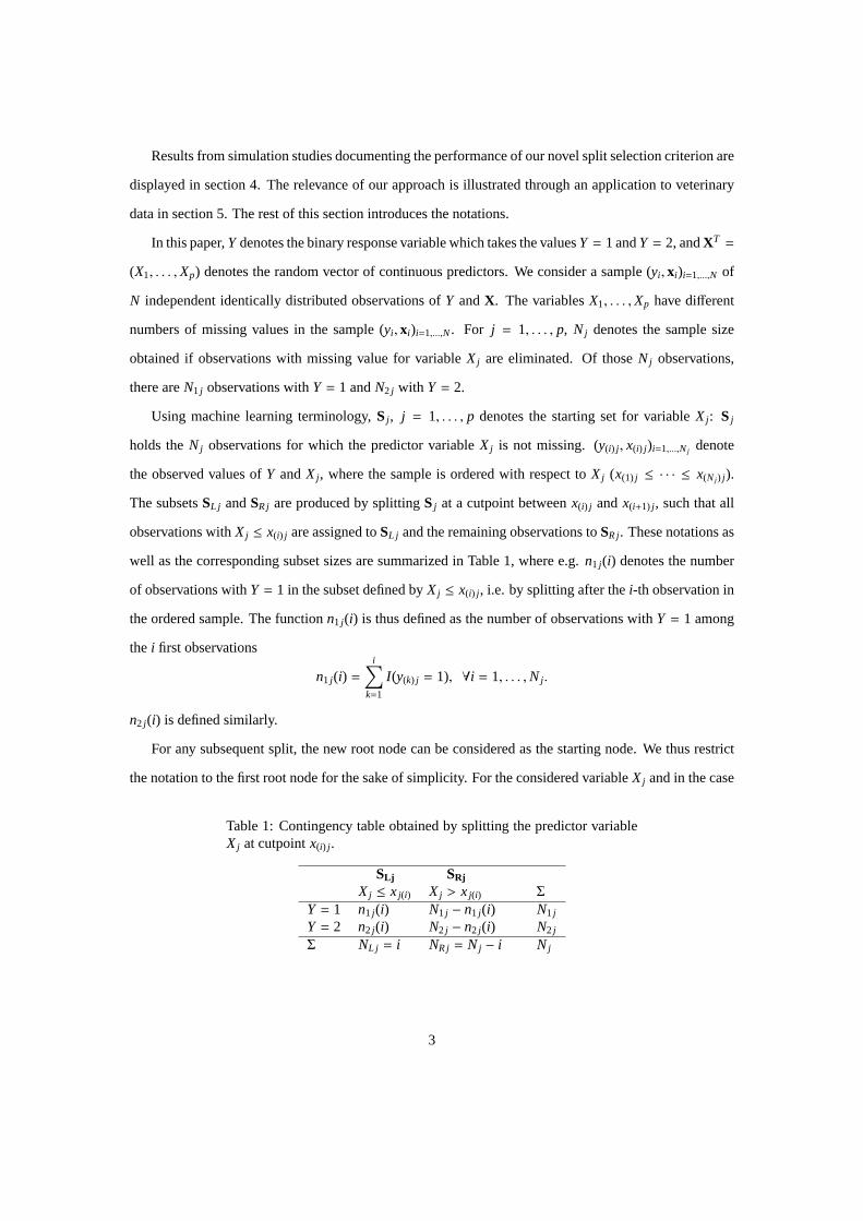
For any subsequent split, the new root node can be considered as the starting node. We thus restrict

the notation to the first root node for the sake of simplicity. For the considered variableX j and in the case

Table 1: Contingency table obtained by splitting the predictor variableX j at cutpointx(i) j .

SLj SRj

X j ≤ x j(i) X j > x j(i) Σ

Y = 1 n1 j(i) N1 j − n1 j(i) N1 j

Y = 2 n2 j(i) N2 j − n2 j(i) N2 j

Σ NL j = i NR j = N j − i N j

3

of a binary responseY, the widely used Gini Index ofSj is the impurity measure defined as

G j = 2N2 j

N j

(1− N2 j

N j

).

GL j andGR j are defined similarly. The Gini gain produced by splittingSj at x(i) j into SL j andSR j is

defined as

∆G j(i) = G j −(NL j

N jGL j +

NR j

N jGR j

)

= G j −(

iN j

GL j +N j − i

N jGR j

).

Obviously, the ’best’ split according to the Gini gain criterion is the split with the largest Gini gain, i.e.

with the largest impurity reduction. The most usual approach for binary split and variable selection in

classification trees consists of the following successive steps:

1. determine the maximal Gini gain∆G jmax over all possible cutpoints for each variableX j , which is

defined as

∆G jmax = maxi=1,...,N−1

∆G j(i),

2. select the variableX j0 with the largest maximal Gini gain:

j0 = arg maxj

∆G jmax.

In many situations, this approach induces variable selection bias: for instance, categorical predictor vari-

ables with many categories are preferred to those with few categories, even if all the predictors are in-

dependent of the response. Variable selection bias occurring when the Gini index is used as a selection

criterion is studied in the next section.

2 Variable selection bias

In this section, empirical evidence for variable selection bias with the Gini gain criterion is reviewed

from the literature. We then outline three important sources of variable selection bias, estimation bias

4

and variance and a multiple comparisons effect, in order to give a comprehensive statistical explanation

of selection bias in different settings.

2.1 Empirical evidence for variable selection bias

Several simulation studies have been conducted to provide empirical evidence for variable selection bias

in different recursive partitioning algorithms (cp. e.g. White and Liu, 1994; Kononenko, 1995; Loh and

Shih, 1997). In this section, we review the experimental design and results of two exemplary studies.

These studies compare the variable selection performance of the Gini gain to that of other splitting criteria.

Together, they cover the main aspects of variable selection bias. The simulation studies in Kim and Loh

(2001) focus on binary splits with the Gini criterion used e.g. inCART (Breiman et al., 1984), while Dobra

and Gehrke (2001) treat the case of multiway splits used in theC4.5 algorithm (Quinlan, 1993), but, in

contrast toC4.5, with the Gini gain as splitting criterion.

In their simulation study, Kim and Loh (2001) vary both the number of categories in categorical

predictor variables and the number of missing values in continuous predictor variables in a binary splitting

framework. Their results show strong variable selection bias towards variables with many categories and

variables with many missing values. On the other hand, Dobra and Gehrke (2001) vary the number of

categories in categorical splitting variables in the case of multiway splitting. In this framework, the Gini

gain does not depend on an optimally selected binary partition of the considered predictor variable, since

the root node is always split into as many nodes as there are categories in the predictor. Dobra and

Gehrke (2001) also observe variable selection bias towards variables with more categories in this context.

However, note that the underlying mechanism causing variable selection bias in favor of variables with

many categories is different in binary and multiway splitting as outlined below.

In the next section, we address three important factors that largely explain the selection bias occurring

with the Gini gain in the different experimental settings.

2.2 Estimation effects

The first two sources of variable selection bias can be considered as ‘estimation effects’: the classical

Gini index used in machine learning can be considered as an estimator of the true entropy. The bias and

the variance of this estimator tend to induce selection bias.

5

2.2.1 Bias

The empirical Gini IndexG used in machine learning can be considered as a plug-in estimator of a ‘true’

underlying Gini Index

G = 2p(1− p),

wherep denotes the probabilityp = P(Y = 2). Under the null-hypothesis that the considered predictor

variableX is uninformative, the class probability is equal to the overall class probability in all subsets.

Using this terminology, the ‘true’ Gini IndexG is a function of the true class probabilityp, whereas

the empirical Gini IndexG is a nonlinear function of the Maximum-Likelihood estimator of the class

probability p, which is the relative class frequency:

G = 2p(1− p)

= 2N2

N(1− N2

N)

From Jensen’s inequality we expect the empirical Gini IndexG to underestimate the true Gini Index

G, and accordingly find:

E(G) = E(2p(1− p))

= 2

E(N2

N) − E(

N22

N2)

, whereN2 ∼ B(N, p)

= 2

(p− p2 +

1N

p(1− p)

)

=N − 1

NG.

Thus, the empirical Gini IndexG underestimates the true Gini Index by factorN−1N :

Bias(G) = −G/N.

The same holds for the Gini indicesGL andGR obtained for the child nodes created by binary splitting

in variableX.

6

The expected value of the Gini gain∆G for fixed NL andNR is then

E(∆G) = G − NLN GL − NR

N GR

= G − GN − NL

N GL + NLN

GLNL− NR

N GR + NRN

GRNR

= GN

=2p(1−p)

N .

The derivation of the expected value of the Gini gain corresponds to that of Dobra and Gehrke (2001)

adopted for binary splits. However, the authors do not elaborate on the interpretation as an estimation bias

induced by the plug-in estimation based on a limited sample size, which we find crucial for understanding

the bias mechanism:

Under the null-hypothesis of an uninformative predictor variable, the ’true’ Gini gain∆G equals 0.

Thus,∆G has a positive bias, that increases with decreasing sample sizeN. When the predictor variables

X j , j = 1, . . . , p, have different sample sizesN j , this bias tends to favor variables with smallN j , i.e.

variables with many missing values.

The same principle applies in classification tree algorithms with multiway splits for categorical pre-

dictors. In this case, the bias increases with the number of categories of the splitting variable: for each

additionally created node, the bias increases by addingGN to the bias derived above. Figuratively speak-

ing, if the overall sample size is divided into several small samples, the estimation from each sample is

inferior and this adds to the overall bias. Similar effects appear when other empirical entropy criteria like

the Shannon entropy are used in multiway splitting (cf. Strobl, 2005).

Therefore the estimation bias of empirical entropy criteria such as the empirical Gini gain is a potential

source of variable selection bias in the null case:

• in multiway splitting if variables differ in their number of categories as in the simulation study of

Dobra and Gehrke (2001), or in their number of missing values

• in binary splitting if variables differ in their number of missing values as in part of the simulation

study by Kim and Loh (2001).

7

2.2.2 Variance

After computations (see Appendix), the variance ofG may be written as

Var(G) = 4GN

(12−G) + O(

1N2

).

It gets large whenG is neither very large nor very low, and for small sample sizes. The variance of∆G

also increases with decreasingNL andNR. Therefore, if the predictor variables have different numbers of

missing values and thus different sample sizes,∆Gmax tends to be larger for variables with many missing

values. This ‘variance effect’ again tends to favor variables with many missing values in binary splitting

and many categories in multiway splitting.

In this section, we outlined two possible sources of selection bias affecting binary or multiway split-

ting with categorical or continuous predictor variables. However, there is another mechanism that can

account for the variable selection bias: the effect of multiple comparisons, which is relevant only if the

number of nodes produced in each split is smaller than the number of distinct observations or categories

like in binary splitting.

2.3 Multiple comparisons in cutpoint selection

The common problem of multiple comparisons refers to an increasing type I error-rate in multiple testing

situations. When multiple statistical tests are conducted for the same data set, the chance to make a type

I error for at least one of the tests increases with the number of performed tests. In the context of split

selection, a type I error occurs when a variable is selected for splitting even though it is not informative.

In the case of binary splitting, the number of conducted comparisons for a given predictor variable

increases with the number of possible binary partitions, i.e. with the number of possible cutpoints. For

categorical and ordinal predictor variables the number of cutpoints depends on the number of categories.

If the predictor is continuous, all the values taken in the sample are distinct. The number of possible

cutpoints to be evaluated is thenN − 1, whereN is the sample size. The ‘multiple comparisons effect’

results in a preference of predictor variables with many possible partitions: with many categories (for

categorical and ordinal variables) or few missing values (for continuous variables). However, in the case

of categorical predictors, the ‘multiple comparisons effect’ is only relevant if several different (binary)

8

partitions are evaluated.

In apparent contradiction Dobra and Gehrke (2001) state explicitly that variable selection bias for

categorical predictor variables was not due to multiple comparisons. However, the authors use the Gini

gain for multiway splits with as many nodes as categories in the predictor rather than for binary splits,

which does not correspond to the standardCART algorithm usually associated with the Gini criterion.

The next section gives a summary of all three effects.

2.4 Resume and practical relevance

The simulation results obtained by Kim and Loh (2001) and Dobra and Gehrke (2001) in different settings

and reviewed in section 2.1 may be explained by the three partially counteracting effects outlined in

sections 2.2 and 2.3.

In the binary splitting task of Kim and Loh (2001), the bias towards predictor variables with many

categories is mainly due to the multiple comparison effect: variables with more categories have more

possible binary partitions to be evaluated. In contrast, the bias towards variables with many missing

values observed for the metric variables may be explained by the bias and variance effects: variables with

small sample sizes, for which the Gini gain is overestimated and has large variance, tend to be favored.

In this case the reverse multiple comparisons effect is outweighed.

In the multiway splitting case of Dobra and Gehrke (2001), the bias towards variables with large

number of categories is due to the bias and variance effects, and not due to multiple comparisons.

In practice, the number of categories in categorical variables of nominal and ordinal scales often

depends on arbitrary choices (e.g. in the design of questionnaires), and the number of missing values

in categorical and metric variables depends on unknown missing mechanisms (e.g. if some questions

are more delicate). Thus, it is obvious that variables should not be preferred due to a higher number of

categories or a higher number of missing values.

As cited in the introduction Breiman et al. (1984) noted the multiple comparisons effect evident when

categorical predictors vary in their number of categories. In addition, they claim that their CART approach

can deal particularly well with missing values, because it provides surrogate splits when predictor values

are missing in the test sample. However, for missing predictor values in the learning sample, the CART

algorithm applies an available case strategy when evaluating the variables in split selection, leading to the

9

bias outlined above. This did not strike Breiman et al. (1984) though, because they only spread missing

values randomly over all predictor variables, instead of varying the sample sizes between variables.

In the next section, we suggest an alternative p-value selection criterion based on the Gini index which

corrects for all the types of bias described above.

3 The distribution of the maximally selected

Gini gain

3.1 A p-value based variable and split selection approach

For the case of binary splits, we introduce the maximally selected Gini gain over all possible splits as a

novel unbiased splitting criterion. Maximally selected statistics, e.g. the maximally selectedχ2- statistic

or maximally selected rank statistics, have been the subject of a few tens of papers published mainly in

the journalBiometricsin the last decades, headed by Miller and Siegmund (1982). They are based on the

following idea. Suppose one computes an association measure (e.g. the Gini gain or theχ2- statistic) for

all theN−1 possible cutpoints of the considered continuous predictor and select the cutpoint yielding the

maximal association measure. The distribution of the resulting “maximally selected” association measure

is different from the distribution of the original association measure. In particular, this distribution may

depend on the sample sizeN, causing the selection bias observed in the case of predictors with different

numbers of missing values, and does not account for the deliberate choice of the cutpoint. Possible

penalizations for the choice of the optimal cutpoint in multiple comparisons are Bonferroni adjustments,

which tend to overpenalize (Hawkins, 1997; Shih, 2002, for a review), and the approach of optimally

selected statistics applied here.

Shih (2004) introduces the p-value of the maximally selectedχ2-statistic as an unbiased split selection

criterion for classification trees, and states that for other criteria, e.g. for entropy criteria like the Gini

Index, “the exact methods are yet to be found.”

Dobra and Gehrke (2001) on the other hand claim that p-value based criteria in general reduce the

selection bias in classification trees, and derive an approximation of the distribution of the Gini gain in the

case of multiway splits. However, their approach does not provide a satisfactory split selection criterion

for binary splitting, because it does not incorporate the multiple comparisons effect in cutpoint selection.

10

In the present paper, we propose to correct the variable selection bias occurring with the Gini gain in

binary splitting by using a criterion based on the distribution of the maximally selection Gini gain rather

than the Gini gain itself. In the rest of the paper,F denotes the distribution function of the maximally

selected Gini gain under the null-hypothesis of no association between the predictor and the response,

givenN1 andN2. For simplicity, we use the notation

F(d) = PH0(∆Gmax≤ d).

In a nutshell, our variable and split selection approach consists to:

1. determine∆G jmax for each predictor variablesX j , j = 1, . . . , p,

2. compute the criterionF(∆G jmax) for each variableX j .

3. select the variableX j0 with the largestF(∆G jmax). The split of X j0 maximizing ∆G j0(i) is then

selected.

The rest of this section presents our novel method to determine the distribution functionF. To simplify

the notations, we consider only one predictor variableX with N non-missing independent identically

distributed observations. We proceed using the notations introduced in Section 1, but omit the indexj for

simplicity.

3.2 Outline of the method

Our aim is to derive the distribution of the maximally selected Gini gain over the possible cutpoints of

X, i.e. over all the possible partitions{SL,SR} of the sample, under the null-hypothesis of no association

betweenX andY. The term(y(i), x(i))i=1,...,N denotes the ordered sample (x(1) ≤ · · · ≤ x(N)). The function

n2(i) is defined as the number of observations withY = 2 among thei first observations:

n2(i) =

i∑

k=1

I (y(k) = 2), ∀k = 1, . . . ,N.

Obviously, we haven2(0) = 0 andn2(N) = N2. Our approach to derive the exact distribution function of

the maximally selected Gini gain consists of two independent steps:

11

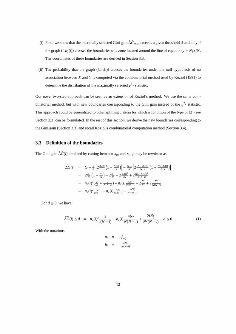
(i) First, we show that the maximally selected Gini gain∆Gmaxexceeds a given threshold if and only if

the graph(i,n2(i)) crosses the boundaries of a zone located around the line of equationy = N2x/N.

The coordinates of these boundaries are derived in Section 3.3.

(ii) The probability that the graph(i,n2(i)) crosses the boundaries under the null hypothesis of no

association betweenX andY is computed via the combinatorial method used by Koziol (1991) to

determine the distribution of the maximally selectedχ2- statistic.

Our novel two-step approach can be seen as an extension of Koziol’s method. We use the same com-

binatorial method, but with new boundaries corresponding to the Gini gain instead of theχ2- statistic.

This approach could be generalized to other splitting criteria for which a condition of the type of (2) (see

Section 3.3) can be formulated. In the rest of this section, we derive the new boundaries corresponding to

the Gini gain (Section 3.3) and recall Koziol’s combinatorial computation method (Section 3.4).

3.3 Definition of the boundaries

The Gini gain∆G(i) obtained by cutting betweenx(i) andx(i+1) may be rewritten as

∆G(i) = G − iN

[2n2(i)

i

(1− n2(i)

i

)]− N−i

N

[2(N2−n2(i))

N−i

(1− N2−n2(i)

N−i

)]

= 2N2N

(1− N2

N

)− 2N2

N + 2n2(i)2

iN + 2(N2−n2(i))2

N(N−i)

= n2(i)2( 2iN + 2

N(N−i) ) − n2(i) 4N2N(N−i) − 2

N22

N2 + 2N2

2N(N−i)

= n2(i)2 2i(N−i) − n2(i) 4N2

N(N−i) +2iN2

2

N2(N−i) .

Ford ≥ 0, we have:

∆G(i) ≤ d ⇔ n2(i)2 2i(N − i)

− n2(i)4N2

N(N − i)+

2iN22

N2(N − i)− d ≤ 0 (1)

With the notations

ai = 2i(N−i) ,

bi = − 4N2N(N−i) ,

12

we obtain after simple computations that

∆G(i) ≤ d ⇔ n2(i) ∈

−bi −

√8d

i(N−i)

2ai,−bi +

√8d

i(N−i)

2ai

. (2)

We want to derive the distribution function of

∆Gmax = maxi=1,...,n−1

∆G(i)

under the null-hypothesis of no association betweenX andY, i.e. PH0(∆Gmax ≤ d) for anyd ≥ 0. We

have∆Gmax ≤ d if and only if condition (2) holds for alli in 1, . . . ,N − 1, i.e. if and only if the path

(i,n2(i)) remains on or above the graph of the function

lowerd(i) =−bi −

√8d

i(N−i)

2ai

and on or under the graph of the function

upperd(i) =−bi +

√8d

i(N−i)

2ai.

A sufficient and necessary condition for∆Gmax ≤ d is that the graph(i,n2(i)) does not pass through any

point of integer coordinates(i, j) with i = 1, . . . ,N − 1 and

lowerd(i) − 1 ≤ j < lowerd(i),

or

upperd(i) < j ≤ upperd(i) + 1.

Let us denote these points asB1, . . . , Bq and their coordinates as(i1, j1), . . . , (iq, jq), whereB1, . . . , Bq are

labeled in order of increasingi and increasingj within eachi. The exact computation of the probability

that the graph(i,n2(i)) passes through at least one of the pointsB1, . . . , Bq (i.e. that it leaves the boundaries

defined above) under the null-hypothesis of no association betweenX and Y is described in the next

section. As an example, the boundaries are displayed in Figure 1 forN1 = N2 = 50andd = 0.1.

13

0 20 40 60 80 100

020

4060

8010

0

obtained boundaries

i

N2(

i)

Figure 1: Boundaries as defined in Section 3.3 for an example withN1 = N2 = 50and d=0.1

3.4 Koziol’s combinatorial approach

Under the null-hypothesis of no association betweenX andY, all the possible paths(i,n2(i)) have equal

probability1/(

NN2

). Thus, the probability that the path(i,n2(i)) passes through at least one of the points

B1, . . . , Bq can be computed using a combinatorial approach as described in Koziol (1991). This approach

is based on a Markov representation ofn2(i) as the path of a binomial process with constant probability

of success and with unit jumps, conditional onN2(N) = N2. Here, we follow Koziol’s formulation, which

is also adopted by Boulesteix (2006b) for ordinal variables. LetPs denote the set of the paths from(0,0)

to Bs that do not pass through pointsB1, . . . , Bs−1 andbs the number of paths inPs. Since the setsPs,

s = 1, . . . , q are mutually disjoint,bs, s = 1, . . . , q can be computed recursively as

b1 =(

i1j1

)

bs =(

isjs

)−∑s−1

r=1

(is−irjs− jr

)br , s = 2, . . . , q.

The above formula may be derived based on simple combinatoric considerations. The number of paths

from (0,0) to Bs is obtained as(

isjs

). To obtain the number of paths from(0,0) to Bs that do not pass

through any of theB1, . . . , Bs−1, one has to subtract from(

isjs

)the sum overr = 1, . . . , s−1 of the numbers

of paths from(0,0) to Bs that pass throughBr but not throughB1, . . . , Br−1. For a givenr (r < s), the

number of paths from(0,0) to Br that do not path throughB1, . . . , Br−1 is br and the number of paths from

14

Br to Bs is(

is−irjs− jr

), hence the product

(is−irjs− jr

)br in the sum in the above formula.

The number of paths from(0,0) to (N,N2) that pass throughBs, s = 1, . . . , q but not through

B1, . . . , Bs−1 is then given as (N − is

N2 − js

)bs.

Since all the possible paths are equally likely under the null-hypothesis, the probability that the graph

(i,n2(i)) passes through at least one of the pointsB1, . . . , Bq is simply obtained as

PH0(∆Gmax> d) =

(NN2

)−1 q∑

s=1

(N − is

N2 − js

)bs. (3)

It follows

F(d) = PH0(∆Gmax≤ d) = 1−(

NN2

)−1 q∑

s=1

(N − is

N2 − js

)bs. (4)

We implemented the computation of the boundaries (step (i)) as well as the combinatorial derivation of

F(d) = PH0(∆Gmax≤ d) (step (ii)) in the languageR. As an example, the obtained boundaries are depicted

in Figure 1 forN1 = N2 = 50andd = 0.1.

4 Simulation studies

In this section, simulation studies are conducted to compare the variable selection performance of the

novel p-value criterion derived in Section 3 to that of the standard Gini gain criterion. We consider a

binary response variableY and 5 mutually independent continuous predictor variablesX1,X2,X3,X4,X5.

In the whole simulation study, the binary responseY is sampled from a Bernoulli distribution with prob-

ability of success0.5. The manipulated parameter is the percentage of missing values in the predictor

variableX1, set successively to 0%,20%,40%,60% and 80%. The missing values are inserted completely

at random (MCAR) within variableX1. The sample size is set toN = 100. However, similarly stable

results can be obtained for smaller sample sizes. Three cases are investigated:

• Null case: all the predictor variablesX1,X2,X3,X4,X5 are uninformative, i.e. independent of the

response variable.

• Power case I:X1 is informative andX2,X3,X4,X5 are uninformative.

15

• Power case II:X2 is informative andX1,X3,X4,X5 are uninformative.

For each parameter setting and each case 1000 data sets are generated. For each data set, variable selection

is performed using successively the standard Gini gain and our p-value criterion. For both criteria, the

obtained frequencies of selection of all variables are given in tables. Based on the literature reviewed

in Section 2, we expect the Gini gain criterion to be biased towards the predictor variable with missing

values, regardless of its information content.

4.1 Null case

In the null case study,X1,X2,X3,X4,X5 are sampled from the standard normal distribution.

X j ∼ N(0,1), for j = 1, . . . , 5,

For each percentage of missing values, the obtained frequencies of selection ofX1,X2,X3,X4,X5 over the

1000 simulation runs is given in Table 2 for the Gini gain (left) and the novel p-value criterion (right).

Since the predictor variables are all independent of the responseY, one expects a good criterion to select

X1,X2,X3,X4 andX5 with random choice probability15.

We find that for the Gini gain criterion the selection frequency ofX1 increases with the amount of

missing values, while it decreases for all other variables. In contrast, the p-value criterion shows almost

no variable selection bias. A slight bias may be obtained for large proportions of missing values. This can

be explained by the fact that for very small sample sizes the Gini gain can only take on very few possible

values, and p-value based criteria can be biased if the probability of the criterion to take on a single value

is significantly large (cf. Dobra and Gehrke, 2001). However, this bias is negligible compared to the bias

of the standard Gini gain criterion.

4.2 Power case I

In the first power case study, the four uninformative predictor variablesX2,X3,X4,X5 are sampled from

the standard normal distribution, while the informative predictor variableX1 is sampled from

X1|Y = 1 ∼ N(0,1)

X1|Y = 2 ∼ N(0.5,1).

16

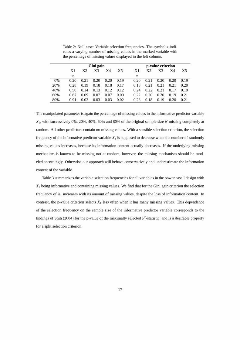
Table 2: Null case: Variable selection frequencies. The symbol◦ indi-cates a varying number of missing values in the marked variable withthe percentage of missing values displayed in the left column.

Gini gain p-value criterionX1 X2 X3 X4 X5 X1 X2 X3 X4 X5◦ ◦

0% 0.20 0.21 0.20 0.20 0.19 0.20 0.21 0.20 0.20 0.1920% 0.28 0.19 0.18 0.18 0.17 0.18 0.21 0.21 0.21 0.2040% 0.50 0.14 0.13 0.12 0.12 0.24 0.22 0.21 0.17 0.1960% 0.67 0.09 0.07 0.07 0.09 0.22 0.20 0.20 0.19 0.2180% 0.91 0.02 0.03 0.03 0.02 0.23 0.18 0.19 0.20 0.21

The manipulated parameter is again the percentage of missing values in the informative predictor variable

X1, with successively 0%, 20%, 40%, 60% and 80% of the original sample sizeN missing completely at

random. All other predictors contain no missing values. With a sensible selection criterion, the selection

frequency of the informative predictor variableX1 is supposed to decrease when the number of randomly

missing values increases, because its information content actually decreases. If the underlying missing

mechanism is known to be missing not at random, however, the missing mechanism should be mod-

eled accordingly. Otherwise our approach will behave conservatively and underestimate the information

content of the variable.

Table 3 summarizes the variable selection frequencies for all variables in the power case I design with

X1 being informative and containing missing values. We find that for the Gini gain criterion the selection

frequency ofX1 increases with its amount of missing values, despite the loss of information content. In

contrast, the p-value criterion selectsX1 less often when it has many missing values. This dependence

of the selection frequency on the sample size of the informative predictor variable corresponds to the

findings of Shih (2004) for the p-value of the maximally selectedχ2-statistic, and is a desirable property

for a split selection criterion.

17

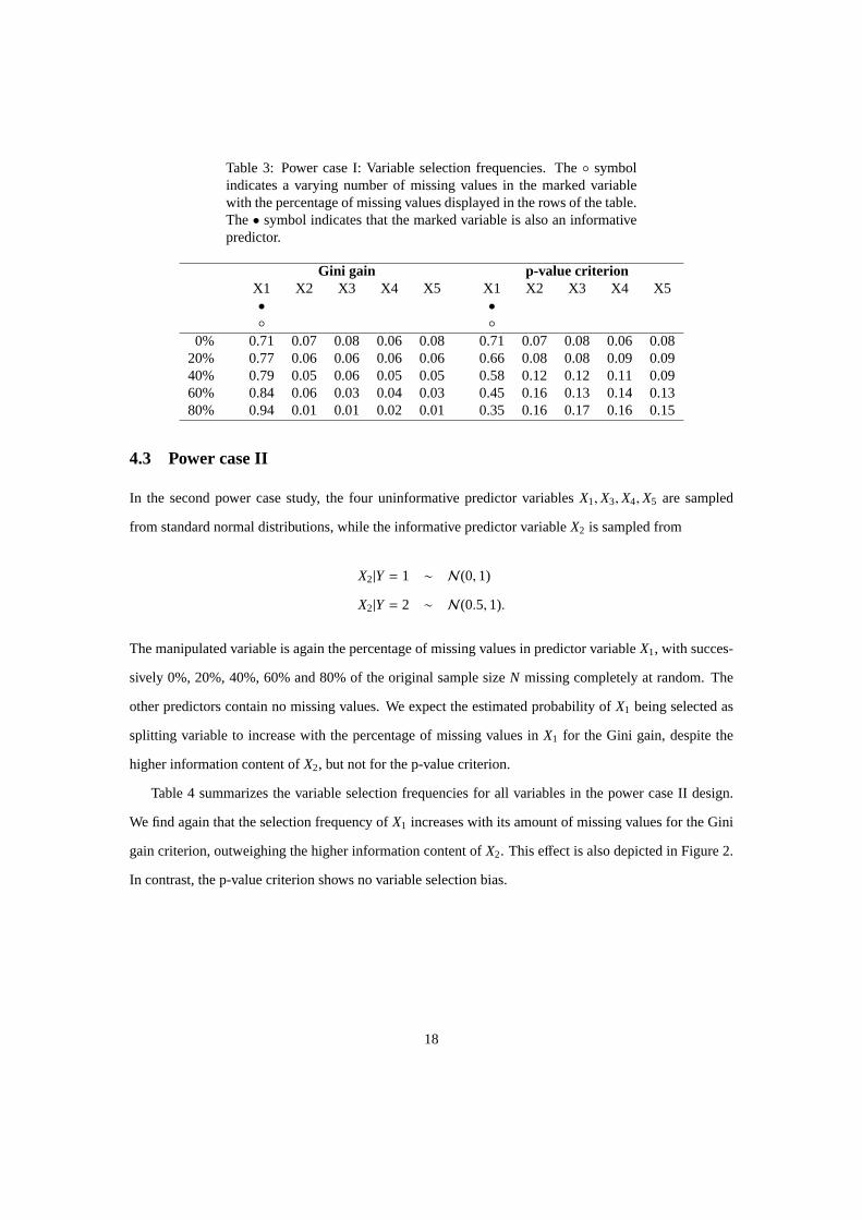
Table 3: Power case I: Variable selection frequencies. The◦ symbolindicates a varying number of missing values in the marked variablewith the percentage of missing values displayed in the rows of the table.The• symbol indicates that the marked variable is also an informativepredictor.

Gini gain p-value criterionX1 X2 X3 X4 X5 X1 X2 X3 X4 X5• •◦ ◦

0% 0.71 0.07 0.08 0.06 0.08 0.71 0.07 0.08 0.06 0.0820% 0.77 0.06 0.06 0.06 0.06 0.66 0.08 0.08 0.09 0.0940% 0.79 0.05 0.06 0.05 0.05 0.58 0.12 0.12 0.11 0.0960% 0.84 0.06 0.03 0.04 0.03 0.45 0.16 0.13 0.14 0.1380% 0.94 0.01 0.01 0.02 0.01 0.35 0.16 0.17 0.16 0.15

4.3 Power case II

In the second power case study, the four uninformative predictor variablesX1,X3,X4,X5 are sampled

from standard normal distributions, while the informative predictor variableX2 is sampled from

X2|Y = 1 ∼ N(0,1)

X2|Y = 2 ∼ N(0.5,1).

The manipulated variable is again the percentage of missing values in predictor variableX1, with succes-

sively 0%, 20%, 40%, 60% and 80% of the original sample sizeN missing completely at random. The

other predictors contain no missing values. We expect the estimated probability ofX1 being selected as

splitting variable to increase with the percentage of missing values inX1 for the Gini gain, despite the

higher information content ofX2, but not for the p-value criterion.

Table 4 summarizes the variable selection frequencies for all variables in the power case II design.

We find again that the selection frequency ofX1 increases with its amount of missing values for the Gini

gain criterion, outweighing the higher information content ofX2. This effect is also depicted in Figure 2.

In contrast, the p-value criterion shows no variable selection bias.

18

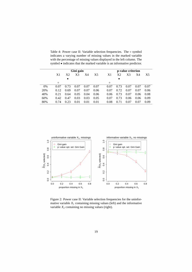
Table 4: Power case II: Variable selection frequencies. The◦ symbolindicates a varying number of missing values in the marked variablewith the percentage of missing values displayed in the left column. Thesymbol• indicates that the marked variable is an informative predictor.

Gini gain p-value criterionX1 X2 X3 X4 X5 X1 X2 X3 X4 X5

• •◦ ◦

0% 0.07 0.73 0.07 0.07 0.07 0.07 0.73 0.07 0.07 0.0720% 0.12 0.69 0.07 0.07 0.06 0.07 0.72 0.07 0.07 0.0640% 0.21 0.64 0.05 0.04 0.06 0.06 0.73 0.07 0.06 0.0860% 0.42 0.47 0.03 0.03 0.05 0.07 0.73 0.06 0.06 0.0980% 0.74 0.23 0.01 0.01 0.01 0.08 0.71 0.07 0.07 0.09

0.0 0.2 0.4 0.6 0.8

0.0

0.2

0.4

0.6

0.8

1.0

uninformative variable X1, missings

proportion missing in X1

P(X

1 se

lect

ed)

+

+

+

+

+

++

+

+

+

+ + + + ++ + + + +

Gini gainp−value opt. sel. Gini Gain

0.0 0.2 0.4 0.6 0.8

0.0

0.2

0.4

0.6

0.8

1.0

informative variable X2, no missings

proportion missing in X1

P(X

2 se

lect

ed)

++

+

+

+

++

+

+

+

+ + + ++

+ + + + +

Gini gainp−value opt. sel. Gini Gain

Figure 2: Power case II: Variable selection frequencies for the uninfor-mative variableX1 containing missing values (left) and the informativevariableX2 containing no missing values (right).

19

5 Application to veterinary data

5.1 Data set

The data were collected in a research farm in the area of Munich, Germany, in 2004. It contains vari-

ous measurements recorded for 51 cows from the week of their first delivery (week 0) until the fourth

week post partum (week 4). The binary response variable of interest take valueY = 1 if the cow shows

signs of minor genital infection andY = 2 if it shows signs of major genital infection or even puerperal

sepsis (childbed fever) and pyometra (uterine suppuration). The potential predictor variables are mea-

sures of body condition, various parameters of the hemogram, milk production, energy consumption and

gynecological indicators that are displayed in Table 5.

The predictor variables vary strongly in their numbers of missing values, e.g., between 0 and 50 in

week 0 and between 0 and 25 in week 4. Some variables contain less than three observations for some of

the weeks, which is obviously not a reasonable sample size in a binary classification task. These variables

were excluded from the analysis for the considered week (week 0: USHR, USHL; week 1: FFS; week 3:

FFS).

The aim of our analysis is to show that the Gini gain and the p-value criterion rank the predictor

variables substantially differently with respect to their number of missing values. In addition, we explore

the explanatory power of the variables that would be selected for the first split with each criterion.

For this exemplary analysis we assume that the missing values are missing completely at random

within each variable.

5.2 Variable selection ranking

The Gini gain criterion and our novel p-value criterion may be used to rank the variables: the least

informative variable is assigned rank 1, and so on. In this section, the rankings of the predictor variables

obtained with the Gini gain criterion and with our novel p-value criterion are compared. Due to selection

bias of the Gini gain towards variables with many missing values, the two rankings are expected to

diverge. The scatterplots of the two rankings are displayed in Figure 3 for each week. The number of

missing values is represented by the circumference of the corresponding point. It can be observed from

the scatterplots that

20

Table 5: Potential predictor variables from the cow data. All variablesare measured on a metric scale but contain strongly varying numbers ofmissing values.

body conditionBCS body condition scoreRFD backfat thickness (mm)MD muscle thickness (mm)

hemogramFFS free fatty acids (µmol/l)Caro carotene (µg/l)Bili bilirubin ( µmol/l)AST aspartate aminotransferase (U/l)CK creatine kinase (U/l)AP alkaline phosphatase (U/l)GLDH glutamate dehydrogenase (U/l)GGT gamma glutamiltransferase (U/l)BHB beta hydroxybutyric acid (mmol/l)IGF1 insulin growth factor 1 (nmol/l)

milk productionMilch milk yield (kg)FettM milk fat (week mean; %)EiM milk protein (week mean; %)FEQ fat-protein-ratioLaktM milk lactose (week mean; %)FLQ fat-lactose-ratioHarnM milk carbamide (week mean; mmol/l)

energy consumptionTMGes dry matter intake total (kg)Eauf energy intake (MJ NEL)EbedM energy requirement (MJ NEL)EbilM energy balance (MJ NEL)

gynecologyUZD cervix diameter (cm)USHR uterine horn diameter right (cm)USHL uterine horn diameter left (cm)

21

- the points deviate noticeably from the bisector,

- the deviation from the bisector is linked to the number of missing values.

Variables with more missing values tend to be ranked higher by the Gini gain criterion than with our

new p-value criterion. Thus, it is useful to consider the unbiased p-value criterion instead of the standard

Gini gain. In classification trees, the variable ranked highest by the chosen criterion is then selected for

splitting. The explanatory power of the variables selected first for splitting is investigated in the following

section.

5.3 Selected splitting variables

In this section, we examine the variables selected for the first split in each week with the standard Gini

gain and with our p-value criterion. When comparing the variables we take into account the number of

missing values, and additionally compute logistic regression models for the binary response and each

selected variable individually. The p-value of the likelihood ratioχ2- test of logistic regression models

does not strictly match with the deterministic bisection approach of classification trees, but can serve as

another indicator of the explanatory power of the selected variables. The results are summarized in Table

6.

We find in Table 6 that the Gini gain criterion systematically prefers variables with high numbers

of missing values. For example, the variable UZD selected by the Gini gain in week 0 has 39 missing

values and only 12 observed values. It should thus be treated with caution. In contrast, the variables

selected by our p-value criterion do not have any or have only few missing values. Through all weeks

the p-values of the logistic regression model (abbreviated by LRM) are lower for the variables selected

by our p-value criterion than for those selected by the Gini gain criterion in each week. This indicates a

higher explanatory power of the variables selected by our p-value criterion in this data set.

Moreover, our p-value criterion may be used as follows as a stopping rule when constructing a clas-

sification tree: We suggest to fix a threshold for the p-value criterion, e.g. 0.95. The considered node is

split only if the p-value criterion of the selected variable exceeds this threshold.

In this example the split with the selected variable would be conducted for weeks 0 through 3 (with

the level again indicated by the * and ** symbols); only in week 4 the split does not produce enough

impurity reduction and is omitted if the threshold is fixed at 0.95. If the threshold was set to .99 the

22

0 5 10 15 20 25 30

05

1015

2025

30

week 0

rank ( Gini Gain )

rank

( p

−va

lue

opt.

sel.

Gin

i Gai

n )

0 5 10 15 20 25 30

05

1015

2025

30

week 1

rank ( Gini Gain )

rank

( p

−va

lue

opt.

sel.

Gin

i Gai

n )

0 5 10 15 20 25 30

05

1015

2025

30

week 2

rank ( Gini Gain )

rank

( p

−va

lue

opt.

sel.

Gin

i Gai

n )

0 5 10 15 20 25 30

05

1015

2025

30

week 3

rank ( Gini Gain )

rank

( p

−va

lue

opt.

sel.

Gin

i Gai

n )

0 5 10 15 20 25 30

05

1015

2025

30

week 4

rank ( Gini Gain )

rank

( p

−va

lue

opt.

sel.

Gin

i Gai

n )

Figure 3: Rank obtained with the new p-value criterion vs. rank ob-tained with the Gini gain. The circumference of each point is propor-tional to number of missing values in the predictor.

23

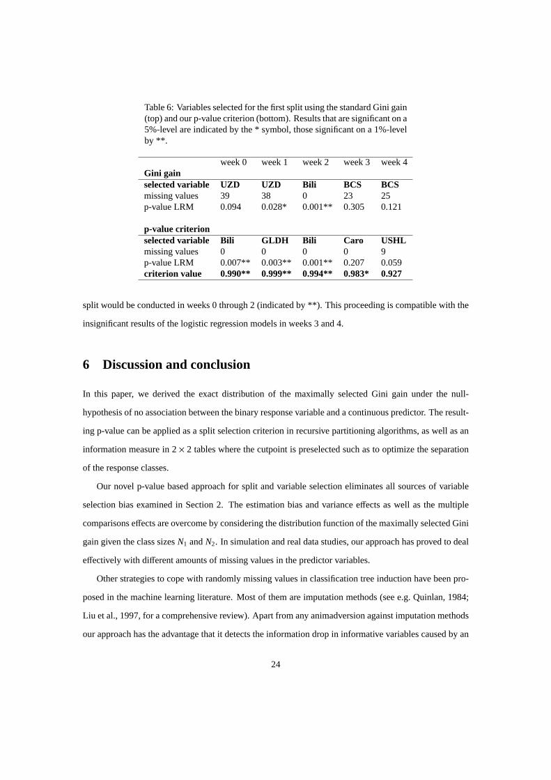
Table 6: Variables selected for the first split using the standard Gini gain(top) and our p-value criterion (bottom). Results that are significant on a5%-level are indicated by the * symbol, those significant on a 1%-levelby **.

week 0 week 1 week 2 week 3 week 4Gini gainselected variable UZD UZD Bili BCS BCSmissing values 39 38 0 23 25p-value LRM 0.094 0.028* 0.001** 0.305 0.121

p-value criterionselected variable Bili GLDH Bili Caro USHLmissing values 0 0 0 0 9p-value LRM 0.007** 0.003** 0.001** 0.207 0.059criterion value 0.990** 0.999** 0.994** 0.983* 0.927

split would be conducted in weeks 0 through 2 (indicated by **). This proceeding is compatible with the

insignificant results of the logistic regression models in weeks 3 and 4.

6 Discussion and conclusion

In this paper, we derived the exact distribution of the maximally selected Gini gain under the null-

hypothesis of no association between the binary response variable and a continuous predictor. The result-

ing p-value can be applied as a split selection criterion in recursive partitioning algorithms, as well as an

information measure in2× 2 tables where the cutpoint is preselected such as to optimize the separation

of the response classes.

Our novel p-value based approach for split and variable selection eliminates all sources of variable

selection bias examined in Section 2. The estimation bias and variance effects as well as the multiple

comparisons effects are overcome by considering the distribution function of the maximally selected Gini

gain given the class sizesN1 andN2. In simulation and real data studies, our approach has proved to deal

effectively with different amounts of missing values in the predictor variables.

Other strategies to cope with randomly missing values in classification tree induction have been pro-

posed in the machine learning literature. Most of them are imputation methods (see e.g. Quinlan, 1984;

Liu et al., 1997, for a comprehensive review). Apart from any animadversion against imputation methods

our approach has the advantage that it detects the information drop in informative variables caused by an

24

increasing number of missing values.

Our p-value based approach may be applied to other common selection criteria such as the deviance

(also called cross-entropy). In future research, one could also work on a generalization to ordinal and

categorical predictors using the boundaries defined in Boulesteix (2006b) and Boulesteix (2006a) for use

in classification trees. In this context, our p-value criterion would address the problem of missing values

and the problem of different numbers of categories simultaneously, in contrast to theR functionrpart

which handles only the problem of missing values in a separate preliminary function, but is biased with

respect to different numbers of categories.

Another advantage of our method is that it is based on the Gini index, with possible extensions to

other popular impurity measures. These easily tangible impurity measures are more attractive to applied

scientists without a strong statistical background than classical test statistics as split selection criteria.

Our criterion can replace the Gini Gain criterion in the traditional “greedy search” approach ofCART,

the intuitiveness of which has played a crucial role in making classification trees understandable and

attractive to a broad scientific community.

Different authors argue along the lines of Loh and Shih (1997), who state that the key to avoiding

variable selection bias is to separate the process of variable selection from that of cutpoint selection. The

resulting algorithmsQUEST (Loh and Shih, 1997) andCRUISE (Kim and Loh, 2001) employ association

test statistics (of ANOVA F-Test for metric predictors and of theχ2-test for categorical predictors) for

variable selection. The split is selected subsequently using discriminant analysis techniques. Hothorn,

Hornik, and Zeileis (2005) critically discuss this approach and propose a more elegant conditional infer-

ence approach.

However, we argue that, in order to achieve unbiased variable selection in classification trees, it is

neither necessary to give up the popular impurity measures, nor to give up the greedy approach that

attracted such a diverse group of applicants with varying statistical knowledge. Giving up the greedy

search approach of the traditional recursive partitioning algorithms for an advanced statistical modeling

approach might, as an unwanted side effect, result in leaving those applicants with a weaker statistical

background behind - with easy to handle but biased classification trees.

Using a p-value criterion based on the Gini index, we address efficiently the problem of selection bias

but preserve the simplicity of traditional classification trees with binary splits. In addition, the p-value

might provide a statistically sound stopping criterion. As all exact procedures, our method becomes

25

computationally intensive for large samples but can handle very small samples. It could be integrated

into any traditional recursive partitioning algorithm and might thus prove both manageable and useful for

applied scientists, as demonstrated in the veterinary example.

Acknowledgements

The authors would like to thank Prof. Dr. R. Mansfeld and his Ph.D. student M. Schmaußer from the

veterinary faculty of the Ludwig-Maximilians-University Munich for providing the veterinary data.

References

Boulesteix, A. L. (2006a). Maximally selected chi-square statistics and binary splits of nominal variables.

Biometrical Journal 48.

Boulesteix, A. L. (2006b). Maximally selected chi-square statistics for ordinal variables.Biometrical

Journal 48.

Breiman, L., J. Friedman, R. Olshen, and C. Stone (1984).Classification and Regression Trees. New

York: Chapman and Hall.

Dobra, A. and J. Gehrke (2001). Bias correction in classification tree construction. InProceedings of the

Seventeenth International Conference on Machine Learning, pp. 90–97. Morgan Kaufmann.

Hawkins, D. M. (1997). Firm: Formal inference based recursive modelling.Technical Report. University

of Minessota..

Hothorn, T., K. Hornik, and A. Zeileis (2005). Unbiased recursive partitioning: A conditional inference

framework.

Kim, H. and W. Loh (2001). Classification trees with unbiased multiway splits.96, 589–604.

Kononenko, I. (1995). On biases in estimating multi-valued attributes. InProceedings of the Fourteenth

International Joint Conference on Artificial Intelligence, pp. 1034–1040.

Koziol, J. A. (1991). On maximally selected chi-square statistics.Biometrics 4, 1557–1561.

26

Liu, W., A. White, S. Thompson, and M. Bramer (1997). Techniques for dealing with mssing values in

classificaton. InAdvances in Intelligent Data Analysis (IDA-97), pp. 527–536.

Loh, W. and Y. Shih (1997). Split selection methods for classification trees.Statistica Sinica 7, 815–840.

Miller, R. and D. Siegmund (1982). Maximally selected rank statistics.Biometrics 38, 1011–1016.

Quinlan, J. R. (1984). Induction of decision trees.Machine Learning 1, 81–106.

Quinlan, R. (1993).C4.5: Programms for Machine Learning. San Francisco: Morgan Kaufmann Pub-

lishers Inc.

Shih, Y.-S. (2002). Regression trees with unbiased variable selection.Statistica Sinica 12, 361–386.

Shih, Y.-S. (2004). A note on split selection bias in classification trees.Computational Statistics and

Data Analysis 45, 457–466.

Strobl, C. (2005). Variable selection in classification trees based on imprecise probabilities. In Coz-

man, Nau, and Seidenfeld (Eds.),Proceedings of the Fourth International Symposium on Imprecise

Probabilities and their Applications, pp. 340–348.

White, A. and W. Liu (1994). Bias in information based measures in decision tree induction.Machine

Learning 15, 321–329.

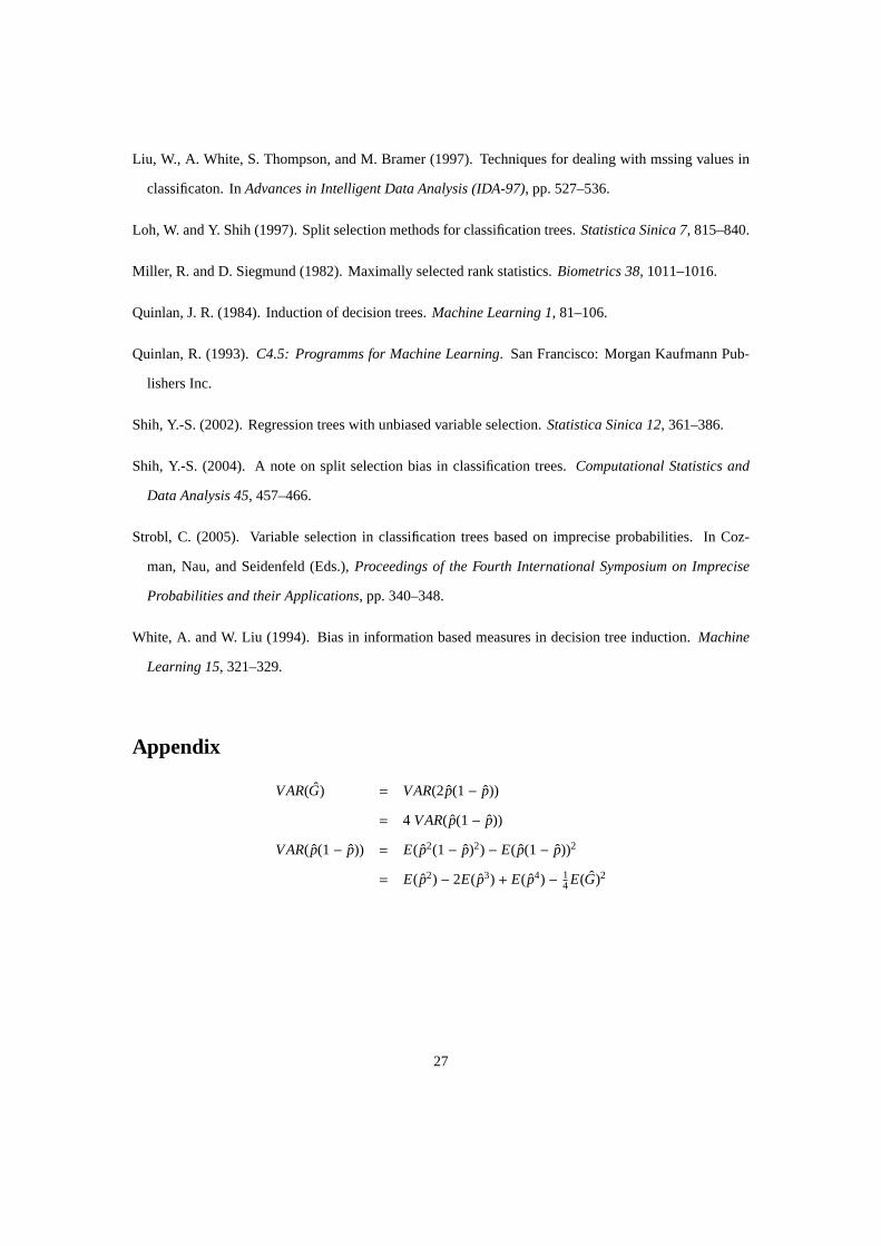
Appendix

VAR(G) = VAR(2p(1− p))

= 4 VAR(p(1− p))

VAR(p(1− p)) = E(p2(1− p)2) − E(p(1− p))2

= E(p2) − 2E(p3) + E(p4) − 14E(G)2

27

We compute the four terms successively.

E(p2) = 1N2 E(x2), wherex ∼ B(N, p)

=pN + p2 − p2

N

= p2 +p(1−p)

N

−2E(p3) = −2( 1N3 E(x3)), wherex ∼ B(N, p)

= −2(3p2

N + p3 − 3p3

N + O( 1N2 ))

= − 6p2

N − 2p3 +6p3

N + O( 1N2 )

E(p4) = 1N4 E(x4), wherex ∼ B(N, p)

=6p3

N + p4 − 6p4

N + O( 1N2 )

− 14E(G)2 = − 1

4(N−1)2

N2 G2

= −G2( 14 − 1

2N ) + O( 1N2 )

Finally,

VAR(p(1− p)) = p2 +p(1−p)

N − 6p2

N − 2p3 +6p3

N +6p3

N + p4 − 6p4

N −G2( 14 − 1

2N ) + O( 1N2 )

= (p2 − 2p3 + p4)(1− 6N ) + G

2N −G2( 14 − 1

2N ) + O( 1N2 )

= G24 (1− 6

N ) + G2N −G2(1

4 − 12N ) + O( 1

N2 )

= G2N (− 6

4 + 12) + G

2N + O( 1N2 )

= GN ( 1

2 −G) + O( 1N2 )

VAR(2p(1− p)) = 4GN ( 1

2 −G) + O( 1N2 )

28