Ultrasound Matrix Imaging. I. The focused reflection ...

HAL Id: hal-03158839https://hal.archives-ouvertes.fr/hal-03158839

Preprint submitted on 4 Mar 2021

HAL is a multi-disciplinary open accessarchive for the deposit and dissemination of sci-entific research documents, whether they are pub-lished or not. The documents may come fromteaching and research institutions in France orabroad, or from public or private research centers.

L’archive ouverte pluridisciplinaire HAL, estdestinée au dépôt et à la diffusion de documentsscientifiques de niveau recherche, publiés ou non,émanant des établissements d’enseignement et derecherche français ou étrangers, des laboratoirespublics ou privés.

Ultrasound Matrix Imaging. I. The focused reflectionmatrix and the F-factor

William Lambert, Laura Cobus, Mathias Fink, Alexandre Aubry

To cite this version:William Lambert, Laura Cobus, Mathias Fink, Alexandre Aubry. Ultrasound Matrix Imaging. I. Thefocused reflection matrix and the F-factor. 2021. �hal-03158839�

Ultrasound Matrix Imaging. I. The focused reflection matrix and the F -factor.

William Lambert,1, 2 Laura A. Cobus,1, 3 Mathias Fink,1 and Alexandre Aubry1, ∗

1Institut Langevin, ESPCI Paris, CNRS, PSL University, 1 rue Jussieu, 75005 Paris, France2SuperSonic Imagine, Les Jardins de la Duranne,

510 Rue Rene Descartes, 13857 Aix-en-Provence, France3Dodd-Walls Centre for Photonic and Quantum Technologies and Department of Physics,

University of Auckland, Private Bag 92019, Auckland 1010, New Zealand

This is the first article in a series of two dealing with a matrix approach for aberration quantifi-cation and correction in ultrasound imaging. Advanced synthetic beamforming relies on a doublefocusing operation at transmission and reception on each point of the medium. Ultrasound matriximaging (UMI) consists in decoupling the location of these transmitted and received focal spots. Theresponse between those virtual transducers form the so-called focused reflection matrix that actuallycontains much more information than a raw ultrasound image. In this paper, a time-frequency anal-ysis of this matrix is performed, which highlights the single and multiple scattering contributions aswell as the impact of aberrations in the monochromatic and broadband regimes. Interestingly, thisanalysis enables the measurement of the incoherent input-output point spread function at any pixelof this image. A focusing criterion can then be built, and its evolution used to quantify the amountof aberration throughout the ultrasound image. In contrast to the standard coherence factor usedin the literature, this new indicator is robust to multiple scattering and electronic noise, therebyproviding a highly contrasted map of the focusing quality. As a proof-of-concept, UMI is appliedhere to the in-vivo study of a human calf, but it can be extended to any kind of ultrasound diagnosisor non-destructive evaluation.

I. INTRODUCTION

To investigate soft tissues in ultrasound imaging, a se-quence of incident waves is used to insonify the medium.Inside the medium, the waves encounter short-scalefluctuations of acoustic impedance, generating back-scattered echoes that are used to build an ultrasoundimage. Conventionally, this estimation of the medium re-flectivity is performed using the process of delay-and-sum(DAS) beamforming, which relies on a coherent summa-tion over all the measured back-scattered echoes gener-ated by any point of the medium. Each echo is selected bycomputing the time-of-flight associated with the forwardand return travel paths of the ultrasonic wave betweenthe probe and the image voxel. From a physical point ofview, time delays in transmission are used to concentratethe ultrasound wave on a focal area whose size is ide-ally only limited by diffraction. Time delays at receptionselect echoes coming from this excited area. This pro-cess falls into the so-called confocal imaging techniques,meaning that, for each point of the image, a double fo-cusing operation is performed.

The critical step of computing the time-of-flight foreach insonification and each focal point is achieved inany clinical device by assuming the medium as homo-geneous with a constant speed of sound. This assump-tion is necessary in order to achieve the rapidity requiredfor real-time imaging; however, it may not be valid forsome configurations in which long-scale fluctuations ofthe medium speed of sound impact wave propagation [1].In soft tissues, such fluctuations are around 5%, as the

∗ [email protected]

speed of sound typically ranges from 1400 m/s (e.g. fattissues) to 1650 m/s (e.g. skin, muscle tissues) [2]. Insuch situations, the incident focal spot spreads beyondthe diffraction-limited area, the exciting pressure fieldat this focusing point is reduced, and undesired back-scattered echoes are generated by surrounding areas. Inreception, the coherent summation is not optimal as itmixes echoes which originate from a distorted focal spot.These aberrating effects can strongly degrade the imageresolution and contrast. For highly heterogeneous me-dia, such aberrations may impact the diagnosis of themedical exam or limit the capability to image some or-gans. A classic example of this effect is liver imaging ofdifficult-to-image patients, in which the probe is placedbetween the ribs. Because the ultrasonic waves musttravel through successive layers of skin, fat, and mus-cle tissue before reaching the liver, both the incident andreflected wave-fronts undergo strong aberrations, distort[3].

To assess the quality of focus and monitor the conver-gence of aberration correction techniques, Mallart andFink [4] introduced a focusing parameter C, known asthe coherence factor in the ultrasound community [5].Based on the van Cittert-Zernike theorem, this indicatoris linked to the spatial coherence of the back-scatteredfield measured by the probe for a focused transmit beam.This method assumes that images are dominated by ul-trasonic speckle – a grainy, noise-like texture which isgenerated by a medium of random reflectivity. This as-sumption is in fact often valid in medical ultrasound,where soft tissues are composed of randomly distributedscatterers that are unresolved at ultrasonic frequencies.In that case, each transmitted focusing wave excites anensemble of scatterers which are randomly distributed

2

within the focal spot. The back-scattered wavefront re-sults from the random superposition of the echoes gen-erated by each of those scatterers. If the focus is per-fect, the time delays used to focus (in transmission andin reception) are exactly the same as the actual round-trip time-of-flight of the waves which arrive at, and arebackscattered by, scatterers located within the resolutioncell. The spatial coherence of the received signal is thenmaximal, and the associated coherence factor C tendstowards 2/3 in the speckle regime. A decrease in thequality of focus is matched by a decrease in C; thus, thisindicator is popular in the literature for the evaluation ofultrasonic focusing quality.

Very recently, ultrasound matrix imaging (UMI) hasbeen proposed for a quantitative mapping of aberrationsin ultrasound imaging [6]. Experimentally, the first stepin this approach is to record the reflection matrix asso-ciated with the medium to be imaged. This matrix con-tains the response of the medium recorded by each trans-ducer of the probe, for a set of illuminations. Dependingon the problem one is facing, this matrix can be investi-gated in different bases. Here, for imaging purposes, thereflection matrix will be projected into a focused basis.In contrast with conventional ultrasound imaging thatrelies on confocal beamforming, the idea here is to ap-ply independent focused beamforming procedures at theinput and output of the reflection matrix. This processyields a focused reflection (FR) matrix that contains theresponses between virtual transducers synthesized fromthe transmitted and received focal spots. The FR ma-trix holds much more information on the medium thandoes a conventional ultrasound image. Importantly, theresolution can be assessed locally for any pixel of theimage. By comparing this resolution with the optimaldiffraction-limited one, a new focusing criterion F is in-troduced to assess the local focusing quality, notably inthe speckle regime. While this indicator shows some sim-ilarities with the coherence factor introduced by Mallartand Fink [4], the parameter F constitutes a much moresensitive probe of the focusing quality. In the quest forlocal correction of distributed aberrations [7–11], this pa-rameter F can be of particular interest as it can play therole of a guide star for any pixel of the ultrasound image.More generally, the FR matrix is a key operator for imag-ing applications [11–15]. The accompanying article [16]will present in details a matrix method of aberration cor-rection in which the FR matrix plays a pivotal role.

The current paper describes the mathematical con-struction and physical meaning of the FR matrix. Inparticular, it is shown how the FR matrix can be ex-ploited to probe the local ultrasound focusing quality,independently of the medium reflectivity. The FR ma-trix was originally introduced in Ref. [6]; here, it is in-vestigated in more detail, and its properties are demon-strated for in-vivo ultrasound imaging of the calf of ahuman subject. First, a time-frequency analysis of theFR matrix is performed, and its mathematical expres-sion is derived rigorously for both the monochromatic

and broadband regimes. The relative weight of single andmultiple scattering contributions, as well as the impactof aberrations, is also discussed for each regime. WhileRef. [6] only considered virtual transducers belonging tothe same transverse plane, here we investigate the im-pulse responses between focusing points located at anydepth [see Fig. 1(a)]. A local incoherent input-outputpoint spread function (PSF) can be extracted from theFR matrix along both the axial and transverse directions.The ratio between the diffraction-limited resolution δx0

and the transverse width wx of the PSF yields the fo-cusing parameter F . The frequency dependence of δx0

is taken into account to obtain a quantitative estimationof the focusing quality with the parameter F . A F -mapis then built and superimposed to the ultrasound image;its comparison with the state-of-the-art C-map shows adrastic gain in terms of contrast. This striking result isdue to the fact that, unlike the coherence factor C, F isrobust to both multiple scattering and electronic noise.

The paper is structured as follows: Section II presentsthe principle of the FR matrix illustrated with in-vivoultrasonic data. In Sec. III, the FR matrix is definedin the monochromatic regime. A 2D local input-outputPSF is extracted from the FR matrix. The manifestationof aberrations, out-of-focus echoes and multiple scatter-ing in this monochromatic PSF is discussed. In Sec. IV,a coherent sum of the monochromatic FR matrices leadsto a broadband FR matrix. This operation, which isequivalent to a time-gating process, suppresses contri-butions from out-of-focus reflectors and from multiplescattering events equally. In Sec. VI, a time-frequencyanalysis of the FR matrix is performed and shows, inparticular, the impact of absorption and scattering onthe FR matrix as a function of depth and frequency.In Sec. VII, a focusing parameter F is obtained bycomparing the experimentally-measured PSD width withthe ideal, diffraction-limited one. It is shown that thefrequency-dependence of F should be taken into accountfor a quantitative mapping of the focusing quality. Fi-nally a discussion section outlines the advantages of Fcompared to the coherence factor C widely used in theliterature [4, 5]. Section IX presents conclusions and gen-eral perspectives.

II. EXPERIMENTAL PROCEDURE

UMI begins with an experimental recording of the re-flection matrix, R. In principle, this measurement canbe achieved using any type of illumination (element-by-element [17], focused beams [18], etc.); here, a plane-wave acquisition sequence [19] has been arbitrarily cho-sen. The probe was placed in direct contact with thecalf of a healthy volunteer, orthogonally to the muscularfibers. (This study is in conformation with the declara-tion of Helsinki). The acquisition was performed usinga medical ultrafast ultrasound scanner (Aixplorer Mach-30, Supersonic Imagine, Aix-en-Provence, France) driv-

3

ing a 5− 18 MHz linear transducer array containing 192transducers with a pitch p = 0.2 (SL18-5, SupersonicImagine). The acquisition sequence consisted of trans-mission of 101 steering angles spanning from −25o to25o, calculated for the hypothesis of a tissue speed ofsound of c0 = 1580 m/s [2]. The pulse repetition fre-quency was set at 1000 Hz. The emitted signal was a si-nusoidal burst lasting for three half periods of the centralfrequency fc = 7.5 MHz. For each excitation, the back-scattered signal was recorded by the 192 transducers ofthe probe over a time length ∆t = 80 µs at sampling fre-quency fs = 40 MHz. Acquired in this way, the reflectionmatrix is denoted Ruθ(t) ≡ R(uout, θin, t), where uout de-fines the transverse position of the received transducer,θin, the incident angle of the emitted plane wave and t,the time-of-flight. In the following, the subscripts in andout will denote the transmitting and receiving steps ofthe reflection matrix recording process.

III. REFLECTION MATRIX IN THEFREQUENCY DOMAIN

The next step consists in projecting the reflection ma-trix into a focused basis. This step is greatly simplifiedby performing beamforming operations in the frequencydomain, i.e. applying appropriate phase shifts to all fre-quency components of the received signals in order torealign them at each focal point. A matrix formalismis particularly suitable for this operation, because, inthe frequency domain, the projection of data from theplane-wave or transducer bases to any focal planecan beachieved with a simple matrix product [6].

Consequently, a temporal Fourier transform should befirst applied to the experimentally acquired reflection ma-trix Ruθ(t):

Ruθ(f) =

∫dt Ruθ(t) e

j2πft. (1)

with f the temporal frequency. Physically, the matrixRuθ(f) can be seen as the result of a three-step sequence:

• Insonification of the medium by a set of planewaves. This emission sequence can be describedby a transmission matrix P = [P (r, θ)] definedbetween the plane wave and focused bases. Eachcolumn of this matrix corresponds to the pressurewave-field at each point r = 〈x, z〉 of the mediumwhen a plane wave is emitted form the probe withan angle of incidence θ.

• Scattering of each incident wave by the mediumheterogeneities. This scattering can be modelledby a matrix Γ defined in the focused basis; in thesingle scattering regime, Γ is diagonal and its ele-ments correspond to the medium reflectivity γ(r, f)at frequency f .

• Back-propagation of the reflected waves towardsthe transducers. This step can be described by theGreen’s matrix G = [G(u, r)] between the trans-ducer and focused bases. Each line of this ma-trix corresponds to the wavefront that would berecorded by the array of transducers if a pointsource was introduced at a point r = (x, z) insidethe sample.

Mathematically, the matrix Ruθ(f) can thus be ex-pressed as the following matrix product:

Ruθ(f) = G>(f)× Γ(f)×P(f). (2)

The holy grail for imaging is to have access to the trans-mission and Green’s matrices, P and G. Their inversionor, more simply, their phase conjugation can enable aprojection of the reflection matrix into a focused basis,thereby providing an estimation of the medium’s reflec-tivity γ(r) despite aberrations and multiple scattering.However, these matrices T and G are not directly acces-sible in most imaging configurations.

IV. MONOCHROMATIC FOCUSEDREFLECTION MATRIX

The projection of the reflection matrix into a focusedbasis requires a preliminary step – the definition of trans-mission matrices which model wave propagation from theplane-wave basis, or transducer basis, to any focal point rin the medium. Here, we consider free-space transmissionmatrices P0(f) and G0(f), which correspond to planewaves and two-dimensional (2D) Green’s functions [20]propagating in a fictitious homogeneous medium withconstant speed-of-sound, c0:

P0 (θ, r, f) = exp (ik · r) (3a)

= exp [ik0 (z cos θ + x sin θ)],

G0 (r, u, f) = − i4H(1)

0

(k0

√(x− u)2 + z2

). (3b)

with k0 = 2πf/c0 the wave number. These transmissionmatrices are then used to beamform the reflection matrixin transmission and reception:

Rrr(f) = G∗0 (f)×Ruθ(z)×P†0 (f) , (4)

where the symbols ∗, † and × stand for phase conju-gate, transpose conjugate and matrix product, respec-

tively. Each row of P†0 = [P ∗0 (θin, rin)]T defines the com-bination of plane waves that should be applied to focus ateach input focusing point rin = {xin, zin}, at frequency f .Similarly, each column of G∗0 = [G∗0(uout, rout)] containsthe amplitude and phase that should be applied to thesignal received by each transducer uout in order to sumcoherently the echoes coming from the output focusingpoint rout = {xout, zout}. Fig. 1(a) illustrates this matrixfocusing process. Note that, for clarity, the input focus-

4

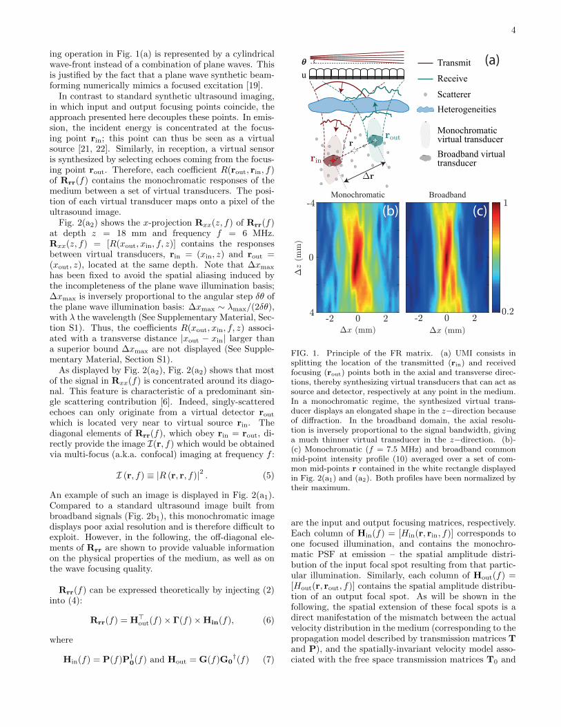
ing operation in Fig. 1(a) is represented by a cylindricalwave-front instead of a combination of plane waves. Thisis justified by the fact that a plane wave synthetic beam-forming numerically mimics a focused excitation [19].

In contrast to standard synthetic ultrasound imaging,in which input and output focusing points coincide, theapproach presented here decouples these points. In emis-sion, the incident energy is concentrated at the focus-ing point rin; this point can thus be seen as a virtualsource [21, 22]. Similarly, in reception, a virtual sensoris synthesized by selecting echoes coming from the focus-ing point rout. Therefore, each coefficient R(rout, rin, f)of Rrr(f) contains the monochromatic responses of themedium between a set of virtual transducers. The posi-tion of each virtual transducer maps onto a pixel of theultrasound image.

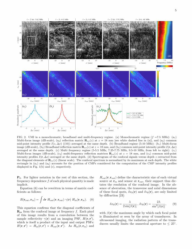
Fig. 2(a2) shows the x-projection Rxx(z, f) of Rrr(f)at depth z = 18 mm and frequency f = 6 MHz.Rxx(z, f) = [R(xout, xin, f, z)] contains the responsesbetween virtual transducers, rin = (xin, z) and rout =(xout, z), located at the same depth. Note that ∆xmax

has been fixed to avoid the spatial aliasing induced bythe incompleteness of the plane wave illumination basis;∆xmax is inversely proportional to the angular step δθ ofthe plane wave illumination basis: ∆xmax ∼ λmax/(2δθ),with λ the wavelength (See Supplementary Material, Sec-tion S1). Thus, the coefficients R(xout, xin, f, z) associ-ated with a transverse distance |xout − xin| larger thana superior bound ∆xmax are not displayed (See Supple-mentary Material, Section S1).

As displayed by Fig. 2(a2), Fig. 2(a2) shows that mostof the signal in Rxx(f) is concentrated around its diago-nal. This feature is characteristic of a predominant sin-gle scattering contribution [6]. Indeed, singly-scatteredechoes can only originate from a virtual detector rout

which is located very near to virtual source rin. Thediagonal elements of Rrr(f), which obey rin = rout, di-rectly provide the image I(r, f) which would be obtainedvia multi-focus (a.k.a. confocal) imaging at frequency f :

I (r, f) ≡ |R (r, r, f)|2 . (5)

An example of such an image is displayed in Fig. 2(a1).Compared to a standard ultrasound image built frombroadband signals (Fig. 2b1), this monochromatic imagedisplays poor axial resolution and is therefore difficult toexploit. However, in the following, the off-diagonal ele-ments of Rrr are shown to provide valuable informationon the physical properties of the medium, as well as onthe wave focusing quality.

Rrr(f) can be expressed theoretically by injecting (2)into (4):

Rrr(f) = H>out(f)× Γ(f)×Hin(f), (6)

where

Hin(f) = P(f)P†0(f) and Hout = G(f)G0†(f) (7)

Monochromatic Broadband

u

ScattererHeterogeneities

Monochromaticvirtual transducerBroadband virtualtransducer

Receive

Transmit (a)

(b) (c)

FIG. 1. Principle of the FR matrix. (a) UMI consists insplitting the location of the transmitted (rin) and receivedfocusing (rout) points both in the axial and transverse direc-tions, thereby synthesizing virtual transducers that can act assource and detector, respectively at any point in the medium.In a monochromatic regime, the synthesized virtual trans-ducer displays an elongated shape in the z−direction becauseof diffraction. In the broadband domain, the axial resolu-tion is inversely proportional to the signal bandwidth, givinga much thinner virtual transducer in the z−direction. (b)-(c) Monochromatic (f = 7.5 MHz) and broadband commonmid-point intensity profile (10) averaged over a set of com-mon mid-points r contained in the white rectangle displayedin Fig. 2(a1) and (a2). Both profiles have been normalized bytheir maximum.

are the input and output focusing matrices, respectively.Each column of Hin(f) = [Hin(r, rin, f)] corresponds toone focused illumination, and contains the monochro-matic PSF at emission – the spatial amplitude distri-bution of the input focal spot resulting from that partic-ular illumination. Similarly, each column of Hout(f) =[Hout(r, rout, f)] contains the spatial amplitude distribu-tion of an output focal spot. As will be shown in thefollowing, the spatial extension of these focal spots is adirect manifestation of the mismatch between the actualvelocity distribution in the medium (corresponding to thepropagation model described by transmission matrices Tand P), and the spatially-invariant velocity model asso-ciated with the free space transmission matrices T0 and

5

0 0.5 1

Frequency (MHz)5 7.5 10

(a1) (b1) (c1)

(a2) (b2) (c2)

(a3) (b3) (c3)

(d)

FIG. 2. UMI in a monochromatic, broadband and multi-frequency regime. (a) Monochromatic regime (f =7.5 MHz): (a1)Multi-focus image (dB-scale), (a2) reflection matrix Rxx(z) at z = 18 mm [see white dashed line in (a)], and (a3) commonmid-point intensity profile I(z,∆x) ((10)) averaged at the same depth. (b) Broadband regime (5-10 MHz): (b1) Multi-focusimage (dB-scale), (b2) Broadband reflection matrix Rxx(z) at z = 18 mm, and (b3) common mid-point intensity profile I(r,∆x)averaged at the same depth. (c) Multi frequency regime (5-5.5 MHz, 7.25-7.75 MHz, 9.5-10 MHz, from left to right): (c1)Multi-focus images (dB-scale), (c2) multi-frequency reflection matrices Rxx(z) at z = 18 mm, and (c3) common mid-pointintensity profiles I(r,∆x) averaged at the same depth. (d) Spectrogram of the confocal signals versus depth z extracted fromthe diagonal elements of Rxx(z) (linear scale). The confocal spectrum is normalized by its maximum at each depth. The whiterectangle in (a1) and (a2) accounts for the position of CMPs considered for the computation of the CMP intensity profilesdisplayed in Fig. 1(b) and (c), respectively.

P0. For lighter notation in the rest of this section, thefrequency dependence f of each physical quantity is madeimplicit.

Equation (6) can be rewritten in terms of matrix coef-ficients as follows:

R(rout, rin) =

∫dr Hout(r, rout) γ(r) Hin(r, rin). (8)

This equation confirms that the diagonal coefficients ofRrr form the confocal image at frequency f . Each pixelof this image results from a convolution between thesample reflectivity γ(r) and an imaging PSF, H(r, r′),which is itself a product of the input and output PSFs:H(r, r′) = Hin(r, r′) × Hout(r, r

′). As Hin(r, rin) and

Hout(r, rout) define the characteristic size of each virtualsource at rin and sensor at rout, their support thus dic-tates the resolution of the confocal image. In the ab-sence of aberration, the transverse and axial dimensionsof these focal spots, δx0(r) and δz0(r), are only limitedby diffraction [23]:

δx0(r) =λ

2 sin[β(r)], δz0(r) =

2λ

sin2[β(r)], (9)

with β(r) the maximum angle by which each focal pointis illuminated or seen by the array of transducers. Inultrasound imaging, the radiation pattern of the trans-ducers usually limits the numerical aperture to ≤ 25◦.

6

The virtual transducers thus typically display a charac-teristic elongated shape in the z−direction (δx0 << δz0

), which accounts for the poor axial resolution exhibitedby the monochromatic image in Fig. 2(a1).

V. COMMON MID-POINT INTENSITY

The off-diagonal points in Rrr can be exploited for aquantification of the focusing quality at any pixel of theultrasound image. To that aim, the relevant observableis the intensity profile along each anti-diagonal of Rrr [6]:

I(rm,∆r) = |R(rm + ∆r/2, rm −∆r/2)|2 . (10)

All pairs of points on a given anti-diagonal have thesame midpoint rm = (rout + rin)/2 , but varying spacing∆r = (rout − rin). In the following, I(rm,∆r) is thus re-ferred to as the common-midpoint (CMP) intensity pro-file. To express this quantity theoretically, we first makean isoplanetic approximation in the vicinity of each CMPrm. This means that waves which focus in this regionare assumed to have travelled through approximately thesame areas of the medium, thereby undergoing identicalphase distortions [11, 16]. The input and/or output PSFscan then be considered to be spatially invariant withinthis local region. Mathematically, this means that, in thevicinity of each common mid-point rm, the spatial distri-bution of the input or output PSFs, Hin/out(r, rin/out),only depends on the relative distance between the pointr and the focusing point rin/out, such that:

Hin/out(r, rin/out) = Hin/out(r− rin/out, rm). (11)

We next make the assumption that, as is often the casein ultrasound imaging, scattering is due to a random dis-tribution of unresolved scatterers. Such a speckle scat-tering regime can be modelled by a random reflectivity:

〈γ(r1)γ∗(r2)〉 = 〈|γ|2〉δ(r2 − r1), (12)

where 〈...〉 denotes an ensemble average and δ is the Diracdistribution. By injecting (8), (11) and (12) into (10), thefollowing expression can be found for the CMP intensity:

I(rm,∆r) =

∫dr |Hout (r−∆r/2, rm) |2

|Hin (r + ∆r/2, rm) |2 |γ(r + rm)|2. (13)

To smooth the intensity fluctuations due to the randomreflectivity, a spatial average over a few resolution cellsis required while keeping a satisfactory spatial resolu-tion. To do so, a spatially averaged intensity profileIav(rm,∆r) is computed in the vicinity of each point rm,such that

Iav(rm,∆r) = 〈WL(r− rm)I(r,∆r)〉r (14)

where the symbol 〈...〉r denotes the spatial average and

WL(r) is a spatial window function, such that

WL(r) =

{1 for |r| < L/20 otherwise.

(15)

This spatial averaging process leads to replace |γ(r)|2in the last equation by its ensemble average 〈|γ|2〉.Iav(rm,∆r) then directly provides the convolution be-tween the incoherent input and output PSFs, |Hin|2 and|Hout|2:

Iav(rm,∆r) ∝[|Hin|2

∆r~ |Hout|2

](∆r, rm). (16)

where the symbol∆r~ denotes a spatial convolution over

∆r – the relative position of rin with respect to rout. Notethat this formula only holds in the speckle regime; for aspecular reflector, the CMP intensity profile is equiva-lent to the intensity of the coherent input-output PSF,

|Hin

∆r~ Hout|2 [6]. In either case, this quantity is gives

two interesting pieces of information: firstly, the inten-sity enhancement Iav(rm,0) of the CMP intensity profileat ∆r = 0 is a direct measure of the average overlapbetween virtual source and detector pairs in the isoplan-etic region. Secondly, the spatial extension of the CMPis linked to the lateral and axial dimensions of the inputand output PSFs. In particular, the transverse full widthat half maximum (FWHM) of the CMP, wx(rm), is a di-rect indicator of the focusing quality at each point rm ofthe medium. In the absence of aberrations,

Hin/out(∆x,∆z = 0, rm) = sinc(2π∆x sin [β(rm)] /λ),(17)

where sinc(x) = sin(x)/x, and wx(rm) is roughly equalto the diffraction-limited resolution δx0(rm).

Fig. 1(b) displays an example of a two dimensionalCMP intensity profile. The corresponding cross-sectionof this profile at ∆z = 0 is displayed in Fig. 2(a3). Thiscross-section has been averaged over a set of CMPs con-tained in the white rectangle of Fig. 2(a1). Similarly tothe input/output PSFs Hin and Hout (9), the incoher-

ent input-output PSF |Hin|2∆r~ |Hout|2 displays a cigar-

like shape. However, while its axial FWHM wz(rm) isclose to the diffraction limit (wz(rm) ∼ δz0 ∼ 2.2 mm,with β = 25◦), its transverse FWHM wx(rm) is far frombeing ideal (wx(rm) ∼ 1 mm >> δx0 ∼ 0.25 mm).This poor resolution can be explained by several poten-tial effects: First, long-scale variations of the speed-of-sound can give rise to aberrations that distort the in-put and output PSFs [11]. Second, if there are spuriousechos from out-of-focus scatterers (located above or be-low the focal plane), then the expansion of the result-ing input/beams will be greater than those originatingexactly at the focal plane [Fig. 1(a)]. This will resultin an enlargement of the resulting input/output PSFs.Finally, short-scale heterogeneities may induce multiplescattering events that give rise to an incoherent back-

7

ground in the CMP intensity profile [6]. The prevalenceof multiple scattering events can be estimated from theamount of signal at off-diagonal elements – an incoherentbackground which is a combination of multiple scatter-ing contributions and electronic noise. The contributionsof these two effects can be separated by examining thespatial reciprocity of measured ultrasonic echos, i.e thesymmetry of Rrr [6]. For the FR matrix displayed inFig. 2(a2), the degree of symmetry of the off-diagonalcoefficients of Rrr is close to 50%. Therefore, the inco-herent background of −14 dB in Fig. 2(a3) contains mul-tiple scattering and electronic noise in equal proportion.However, these contributions still constitute a problemfor imaging; in the monochromatic regime under exam-ination here, is it extremely difficult to discriminate be-tween the effects of aberration, multiple scattering, andsingly-scattered echoes taking place out-of-focus. In thenext section, we show that the contributions from multi-ple scattering and from out-of-focus echos can be greatlyreduced via a time-gating operation. This filter improvesthe axial resolution of the ultrasound imaging.

VI. BROADBAND REFLECTION MATRIX

Under the matrix formalism, time gating can be per-formed by building a broadband FR matrix Rrr. In thefollowing, we show that besides improving the axial res-olution and contrast of the ultrasound image, Rrr allowsa clear distinction between the contributions from singleand multiple scattering.

In the frequency domain, the FR matrix is built bydephasing each RF signal in order to make scatteringpaths going through both input and output focal spotsconstructively interfere (4). A coherent sum over theoverall bandwidth ∆f can then be performed to build abroadband FR matrix:

Rrr(∆f) =1

∆f

∫ f+

f−

df Rrr(f) (18)

with f± = fc±∆f/2 and fc the central frequency of theRF signal bandwidth. In our experiment, fc = 7.5 MHzand ∆f = 5 MHz. One row of the broadband FR matrixcorresponds to the situation in which the transmittedwaves are focused at rin, creating a virtual source whilethe virtual detector probes the spatial spreading of thisvirtual source at the expected ballistic time, i.e at timet = 0 in the focused basis [Fig. 1(a)]. Thus, the sum ofmonochromatic FR matrices over the entire bandwidthcan be interpreted as a time-gating operation in whichechos originating from a certain range of times-of-flightare extracted.

With the time-gating applied (18), the axial resolutionof the virtual transducers should be drastically improved[see Fig. 1(a)]. To prove this assertion, we now derive anexpression for the broadband FR matrix within the for-malism of this work. For sake of simplicity and analytical

tractability, paraxial and isoplanatic (11) approximationsare made. The monochromatic PSFs can be decomposedas follows:

Hin/out(r, r′, f) = H in/out(r− r′, rm, f) ej2πf(z−z′)/c

(19)where H in/out represents the envelope of the PSF. Inject-ing (8) and (19) into (18) leads to the following expres-sion for the coefficients of Rrr(∆f) (See SupplementaryMaterial, Section S2.):

R(rout, rin,∆f) =

∫dr ej2πfc(2z−zin−zout)/c

sinc

[π∆f

c(2z − zin − zout)

]Hout(r− rout, rm) γ(r) H in(r− rin, rm). (20)

where we have assumed, in first approximation, thatH in/out is constant over the frequency bandwidth. Theoccurrence of the sinc factor in the integrand of the lastequation shows that, in the broadband regime, the axialresolution δz0 is dictated by the frequency bandwidth,such that

δz0 ∼c

2∆f. (21)

Fig. 2(b1) shows the ultrasound image I(r,∆f) builtfrom the diagonals of Rrr(∆f) (5). The gain in resolu-tion, compared to the original monochromatic image in[Fig. 2(a1)], is clearly visible. While the monochromaticimage displays an elongated speckle that is not very sen-sitive to the structural details of the calf, the coherentsum of (18) drastically improves the axial resolution andcontrast of the image, revealing the micro-architecture ofthe calf tissues.

Fig. 2(b2) shows the cross-section Rxx(∆f, z) of thebroadband FR matrix Rrr(∆f) at depth z = 18 mm [dot-ted white line of Fig. 2(b1)]. Compared to its monochro-matic counterpart [Fig. 2(a2)], the single scattering con-tribution along the diagonal of Rrr is enhanced withrespect to the off-diagonal coefficients. This enhance-ment is due to the time-gating procedure; contributionsfrom scatterers which sit above and below the focal planehave been eliminated, so the remaining singly-scatteredechoes are located near the diagonal of Rrr. Note thatthe multiply-scattered echoes whose time-of-flight differsfrom the ballistic time are also removed in the same pro-portion. The single-to-multiple scattering ratio is thuspreserved through the time gating operation.

The improvement in transverse resolution can also beseen in the broadband CMP intensity profile displayedin Fig. 1(c), and in its cross-section shown in Fig. 2(b3).Compared to the monochromatic regime [Figs. 1(b) and2(a2)], the CMP cross-section now displays a confocal,steep peak on top of a flat multiple scattering back-ground. Surprisingly, although we are in a broadbandregime, the 2D focal spot in Fig. 1(c) still exhibits a

8

cigar-like shape. To understand the reason for this, wenow express the ensemble average of the CMP intensityprofile (19) in the broadband regime under the paraxialapproximation (see Supplementary Section S2):

Iav(rm,∆r,∆f) =A

∆f

∫ f+

f−

df

[|H in|2

∆x~ |Hout|2

](∆r, rm, f),

(22)where A is a constant. Equation 22 shows that, in thebroadband regime, the CMP intensity profile correspondsto the sum over the frequency bandwidth of the inco-

herent input-output PSF |H in|2∆x~ |Hout|2. This explains

why the axial resolution has not been improved by thetime gating process, as it was for the broadband FR ma-trix (Eq. 20). Nevertheless, the CMP intensity evolutionalong ∆x still offers a way to estimate the transverseresolution of the imaging PSF in the broadband regime.Indeed, Fig. 2(b3) shows that the transverse resolutionremains far from being optimized: wx(∆f) ∼ 0.5 mm>> δx0(fc) ∼ 0.25 mm.

In the next section, we aim to develop a better way toevaluate transverse resolution in the broadband regime.We will define a quantitative parameter to measure thefocusing quality at any pixel of the ultrasound image.This observable compares the experimental δx0(∆f) tothe ideal diffraction-limited case. To make our mea-surement quantitative, the theoretical prediction of thediffraction-limited δx0(∆f) should be as accurate as pos-sible; in the following, we work towards this accuracy bydeveloping a theoretical time-frequency analysis of theFR matrix.

VII. TIME-FREQUENCY ANALYSIS OF THEFOCUSED REFLECTION MATRIX

A time-frequency analysis of the FR matrix is requiredto investigate the evolution of absorption and scatteringas a function of frequency. To do so, the coherent sumof the monochromatic FR matrices [Eq. 18] can be per-formed over a smaller bandwidth δf centered on a givenfrequency f :

Rrr(f, δf) =1

δf

∫ f+δf

f−δfdf ′ Rrr(f

′) (23)

We have shown that the axial dimension δz0 of the virtualtransducers is inversely proportional to the frequencybandwidth δf (Eq. 21). Thus, a compromise must to bemade between the spectral and axial resolutions. Here,the following choice has been made: δf = 0.5 MHz andδz0 = 3 mm.

Fig. 2(c) shows the ultrasound images [Fig. 2(c1)], FRmatrices [Fig. 2(c2)] and CMP profiles [Fig. 2(c3)] forthree different frequency bandwidths: 5-5.5 MHz, 7.25-7.75 MHz, 9.5-10 MHz. The axial resolution in eachultrasound image is of course deteriorated compared to

the broadband image [Fig. 2(b1)]; nevertheless, the time-frequency analysis of the FR matrices yields the evolutionof the SNR versus depth and frequency. At z = 18 mm,for instance, the FR matrix at f = 9.75 MHz exhibits atiny confocal intensity enhancement on top of a predom-inant noise background (SNR∼3dB). Conversely, the FRmatrices at f = 5.25 and 7.5 MHz exhibit a CMP in-tensity profile which more closely resembles its broad-band counterpart. This weak SNR at 9.75 MHz can bepartially explained by the finite bandwidth of the trans-ducers (5 − 10 MHz). Interestingly, absorption lossesundergone by ultrasonic waves in soft tissues also havea strong impact on the ultrasound image. Fig. 2(d) il-lustrates the effect of absorption by displaying the spec-trum of the confocal signal,

⟨I(r, f, δf)

⟩x, as a function

of depth. This spectrum shifts towards low frequencies asa function of depth. This frequency shift is characteristicof absorption losses in soft tissue, for which the attenua-tion coefficient is assumed to exhibit a linear dependenceon frequency [2].

The time-frequency analysis of the FR matrix alsoallows the observation of frequency fluctuations inI(r, f, δf) which are not related to absorption. For in-stance, while a bright scatterer [white arrow in Fig. 2(b1)]is clearly visible in the broadband or low frequencyregimes around x = 12.5 mm and z = 18 mm, its pres-ence is not revealed by the FR matrices at higher frequen-cies. A time-frequency analysis can thus be of interestfor characterization purposes, as the frequency responseof bright scatterers is directly related to their size andcomposition.

Whether due to absorption or scattering, the variationof the temporal frequency spectrum of back-scatteredechoes has a strong impact on the local resolution of theultrasound images. In the next section, we show how toincorporate this frequency dependence in the theoreticalexpression of the spatial resolution, in order to establisha more precise quantitative focusing parameter using theCMP intensity profile.

VIII. THE LOCAL FOCUSING CRITERION

In this section, a local focusing criterion is estab-lished for the broadband ultrasound image. For thesake of lighter notation, the dependence of each phys-ical quantity with respect to ∆f is omitted. Aberra-tions caused by medium heterogeneities degrade the res-olution of the ultrasound image and induce a spread-ing of singly-scattered echoes over the off-diagonal coef-ficients of Rrr. In the speckle regime, it is difficult todetermine by eye whether the image is aberrated, andif so, which areas are the most impacted. Interestingly,the transverse width wx(rm) of the CMP intensity pro-file can yield an unambiguous answer to this question.In the speckle regime, this profile yields the convolutionbetween the incoherent input-output PSF averaged overthe frequency bandwidth (Eq. 22). While the incoherent

9

input-output PSF is not exactly equal to the confocalimaging PSF, (Eq. 20), it nevertheless fully captures theimpact of transverse aberrations. It thus constitutes arelevant observable for assessing focusing quality.

A precise measurement of the transverse width of theCMP intensity profile, wx(rm), requires an estimate ofthe background noise level, Ib(rm). In practice, Ib(rm)is computed by averaging the CMP profile away fromthe confocal peak, such that Ib = 〈Iav(rm,∆x)〉|∆x|>wc

,where wc is the overall support of the confocal peak.In the case considered here, wc ∼ 17λc ∼ 3.5 mm (seeFig. 2b3), where λc ≈ 0.21 mm is the central wavelengthdefined at fc = 7.5 MHz. wx(rm) is then deduced as theFWHM of the CMP intensity profile Iav(rm,∆x) aftersubstraction of the background noise Ib(rm).

The width wx(rm) of the imaging PSF is dictated bytwo distinct phenomena: diffraction and aberration. Inthe ideal case (i.e no aberrations), the image resolutionδx0(rm) is only impacted by diffraction and, more pre-cisely, dictated by the angular aperture β(rm) (Eq. 9).The angular aperture tends to decrease decrease at largerdepths and nearer to the edge of the image. In the pres-ence of aberrations, both diffraction and wave-front dis-tortions alter the imaging PSF. In order to provide anindicator that is only sensitive to aberrations, the estima-tor wx(rm) of the image resolution should be comparedto its ideal value δx0(rm) (Eq. 9) at each point of theultrasound image. To do so, a local focusing criterionF (rm) is defined:

F (rm) = δx0(rm)/wx(rm). (24)

To estimate this parameter, the major challenge liesin the determination of the ideal resolution δx0(rm) forbroadband signals. To do so, the frequency spectrum ofthe ultrasound image should be taken into account. Foreach CMP rm, I(rm, f) is an estimation of the desiredfrequency spectrum [Fig. 2(d)]. Equation (9) can thenbe extended to broadband signals by using I(rm, f) as aweighting factor. The expected lateral resolution is thengiven by:

δx0(rm) =

⟨W∆r(r− rm)

∫ f+f−

df I(r, f) δx0(f, r)∫ f+f−

df I(r, f)

⟩r

.

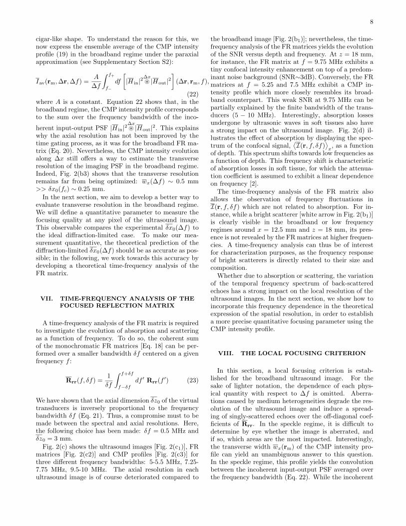
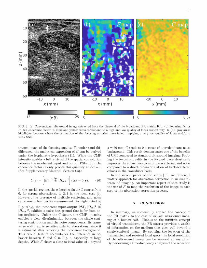
(25)By injecting (25) into (24), the focusing criterion, F (rm),can be computed. Fig. 3(b) displays the focusing crite-rion superimposed onto the conventional B-mode image.The extension of the spatial window W∆r has been set to7λc. While high values of F (F ∼ 1, blue areas) indicategood image reliability, low values of F (F < 0.3, yellowareas) indicate a poor quality of focus and gray areas areassociated with a low SNR. Both yellow and grey areasseem to correspond to blurring of the ultrasound image[Fig. 3a]. Indeed, these areas correspond to the situationin which the estimation of the image resolution has failed,meaning that there is no intensity enhancement of the

close-diagonal coefficients in Rxx(z,∆f). Two comple-mentary reasons can explain this behaviour: Either thesingle scattering contribution is drowned out by a moredominant background noise (caused by multiple scatter-ing processes and electronic noise), or the aberrations areso intense that the confocal spot spreads over an extendedimaging PSF, thereby pushing the single scattering inten-sity at focus below the noise level. Unsurprisingly, thissituation occurs at large depth and in areas where themedium reflectivity is weak. In any case, if a medicaldiagnosis is desired, the features of the ultrasound imagein these areas should be more carefully interpreted.

Fig. 3(b) reveals a poor focusing quality at a shallowdepth that could be due to a mismatch between the speedof sound in the skin, cskin ≈ 1500 − 1700 m/s [24], andour wave velocity model (c0 = 1580 m/s). The ultra-sound images show different structures that are associ-ated with their own speed of sound: (i) muscles tissueswith three different fiber orientations [areas I, II, III onFig. 3(a)]; (ii) two veins located at {x, z} = 12, 5 mmand −5, 33 mm; and (iii) the fibula, located at the bot-tom left of the figure −12, 45 mm. However, finding thelink between quality of focus provided by the focusing cri-terion and the spatial distribution of the speed of soundthroughout the medium is a difficult task that is beyondthe scope of this paper.

IX. DISCUSSION

The study presented here – in-vivo UMI of a humancalf – provides new insights into the construction of theFR matrix and the focusing criterion. Our results arerepresentative of in-vivo ultrasound imaging in whichthe medium under investigation is composed of differ-ent kinds of tissues, which can themselves be heteroge-neous. As the medium is composed of a mix of unresolvedscatterers and specular reflectors, the scattering of ultra-sound varies considerable in space, ranging from areas ofstrong to weak scattering. A direct and important ap-plication of this work would thus be to aid aberrationcorrection by employing the parameter F as a virtualguide star for adaptive focusing techniques. Currently,in the literature in this area, this role is performed bythe coherence factor C [25–27].

Here, to highlight the benefit of our matrix approachwith respect to the state-of-the-art, we build a map ofthe standard coherence factor C for the ultrasound im-age of the human calf. C is equal to the ratio of thecoherent intensity to the incoherent intensity of the re-aligned reflected wave-fronts recorded by the probe foreach input focusing beam [28]. Just as with the calcula-tion of the CMP intensity profile (14), the raw coherencefactor C(rin) is then spatially averaged over overlappingspatial windows to smooth the fluctuations due to therandom reflectivity. The result is mapped onto the ul-trasound image in Fig. 3c. Compared to the F−map(Fig. 3b), the coherence factor C provides a weakly con-

10

z (m

m)

10

20

30

40

50

60-10 0 10

x (mm)

(a)

I

II

III

-10 0 10x (mm)

(c)

(dB)-12 25

10-10 0x (mm)

(b)

0 1 0 0.67

F-map C-map

FIG. 3. (a) Conventional ultrasound image extracted from the diagonal of the broadband FR matrix Rrr. (b) Focusing factorF . (c) Coherence factor C. Blue and yellow areas correspond to a high and low quality of focus respectively. In (b), gray areashighlights location where the estimation of the focusing criterion have failed, implying a very low quality of focus and/or aweak SNR.

trasted image of the focusing quality. To understand thisdifference, the analytical expression of C can be derivedunder the isoplanatic hypothesis (11). While the CMPintensity enables a full retrieval of the spatial convolutionbetween the incoherent input and output PSFs (16), thecoherence factor C only probes this quantity at ∆x = 0(See Supplementary Material, Section S3).:

C(r) =

[|H in|2

∆x~ |Hout|2

](∆x = 0, r). (26)

In the speckle regime, the coherence factor C ranges from0, for strong aberrations, to 2/3 in the ideal case [4].However, the presence of multiple scattering and noisecan strongly hamper its measurement. As highlighted by

Fig. 2(b2), the incoherent input-output PSF, |H in|2∆x~

|Hout|2, exhibits a noise background that is far from be-ing negligible. Unlike the C-factor, the CMP intensityenables a clear discrimination between the single scat-tering contribution and the noise components. Its trans-verse width wx is sensitive only to aberrations, since itis estimated after removing the incoherent background.This crucial feature accounts for the difference in be-havior between F and C in Fig. 3, especially at largedepths. While F shows a close to ideal value of 1 beyond

z = 50 mm, C tends to 0 because of a predominant noisebackground. This result demonstrates one of the benefitsof UMI compared to standard ultrasound imaging: Prob-ing the focusing quality in the focused basis drasticallyimproves the robustness to multiple scattering and noisecompared to a direct cross-correlation of back-scatteredechoes in the transducer basis.

In the second paper of the series [16], we present amatrix approach for aberration correction in in vivo ul-trasound imaging. An important aspect of that study isthe use of F to map the resolution of the image at eachstep of the aberration correction process.

X. CONCLUSION

In summary, we successfully applied the concept ofthe FR matrix to the case of in vivo ultrasound imag-ing of a human calf. Thanks to the intuitive conceptof virtual transducers, the FR matrix provides a wealthof information on the medium that goes well beyond asingle confocal image. By splitting the location of thetransmitted and received focal spots, the local resolutionof the ultrasound image can be assessed at any pixel.By performing a time-frequency analysis of the reflection

11

matrix, the contributions of single and multiple scatter-ing and their impact on the resolution and contrast werecarefully investigated. This time-frequency study of theFR matrix paves the way towards a quantitative charac-terization of soft tissues by measuring parameters suchas the attenuation coefficient or the scattering mean freepath. In the accompanying paper [16], the FR matrixwill be used as a key building block of UMI for a lo-cal aberration correction. Relatedly, a focusing criterionwas defined from the FR matrix in order to quantify theimpact of aberrations on each pixel of the ultrasound im-age. Compared to the coherence factor generally used inthe literature [4, 5], our focusing parameter is much morerobust to noise and multiple scattering. Our focusing pa-rameter is thus promising for use in medical imaging asa reliability index of the ultrasound image. It can alsobe used as a guide star for adaptive focusing techniques,or as a local aberration indicator for UMI [16].

ACKNOWLEDGMENT

The authors wish to thank Victor Barolle, AmauryBadon and Thibaud Blondel whose own research worksin optics and seismology inspired this study. This projecthas received funding from the European Research Coun-cil (ERC) under the European Union’s Horizon 2020research and innovation programme (grant agreementNo. 819261); the Labex WIFI (Laboratory of Excellencewithin the French Program Investments for the Future,ANR-10-LABX-24 and ANR-10-IDEX-0001-02 PSL*).W.L. acknowledges financial support from the SupersonicImagine company. L.C. acknowledges financial supportfrom the European Union’s Horizon 2020 research and in-novation programme under the Marie Sklodowska-Curiegrant agreement No. 744840.

12

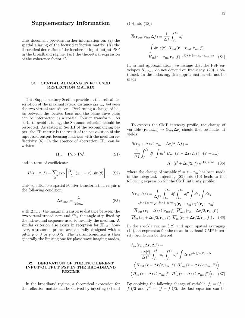
Supplementary Information

This document provides further information on: (i) thespatial aliasing of the focused reflection matrix; (ii) thetheoretical derivation of the incoherent input-output PSFin the broadband regime; (iii) the theoretical expressionof the coherence factor C.

S1. SPATIAL ALIASING IN FOCUSEDREFLECTION MATRIX

This Supplementary Section provides a theoretical de-scription of the maximal lateral distance ∆xmax betweenthe two virtual transducers. Performing a change of ba-sis between the focused basis and the plane wave basiscan be interpreted as a spatial Fourier transform. Assuch, to avoid aliasing, the Shannon criterion should berespected. As stated in Sec.III of the accompanying pa-per, the FR matrix is the result of the convolution of theinput and output focusing matrices with the medium re-flectivity (6). In the absence of aberration, Hin can bewritten:

Hin = P0 ×P0†, (S1)

and in term of coefficients:

H(rin, r, f) =∑θ

exp

[i2π

λ(xin − x) sin(θ)

]. (S2)

This equation is a spatial Fourier transform that requiresthe following condition:

∆xmax =λ

2δθin, (S3)

with ∆xmax the maximal transverse distance between thetwo virtual transducers and δθin the angle step fixed bythe ultrasound sequence used to insonify the medium. Asimilar criterion also exists in reception for Hout; how-ever, ultrasound probes are generally designed with apitch p ∝ λ or p ∝ λ/2. The transmitcondition is thengenerally the limiting one for plane wave imaging modes.

S2. DERIVATION OF THE INCOHERENTINPUT-OUTPUT PSF IN THE BROADBAND

REGIME

In the broadband regime, a theoretical expression forthe reflection matrix can be derived by injecting (8) and

(19) into (18):

R(rout, rin,∆f) =1

∆f

∫ f+

f−

df∫dr γ(r) Hout(r− rout, rm, f)

H in(r− rin, rm, f) ej2πf(2z−zin−zout)/c (S4)

If, in first approximation, we assume that the PSF en-velopes H in/out do not depend on frequency, (20) is ob-tained. In the following, this approximation will not bemade.

To express the CMP intensity profile, the change ofvariable (rin, rout) → (rm,∆r) should first be made. Ityields:

R(rm + ∆r/2, rm −∆r/2,∆f) =

1

∆f

∫ f+

f−

df

∫dr′ Hout(r

′ −∆r/2, f) γ(r′ + rm)

H in(r′ + ∆r/2, f) ej4πfz′/c (S5)

where the change of variable r′ = r− rm has been madein the integrand. Injecting (S5) into (10) leads to thefollowing expression for the CMP intensity profile:

I(rm,∆r) =1

∆f2

∫ f+

f−

df

∫ f+

f−

df ′∫dr1

∫dr2

ej4πfz1/c e−j4πf′z2/c γ(r1 + rm) γ∗(r2 + rm)

Hout (r1 −∆r/2, rm, f) H∗out (r2 −∆r/2, rm, f

′)

H in (r1 + ∆r/2, rm, f) H∗in (r2 + ∆r/2, rm, f

′) . (S6)

In the speckle regime (12) and upon spatial averaging(14), an expression for the mean broadband CMP inten-sity profile can be derived:

Iav(rm,∆r,∆f) =

〈|γ|2〉∆f2

∫ f+

f−

df

∫ f+

f−

df ′∫dr ej4π(f−f ′) z/c

⟨Hout (r−∆r/2, rm, f) H

∗out (r−∆r/2, rm, f

′)⟩

⟨H in (r + ∆r/2, rm, f) H

∗in (r + ∆r/2, rm, f

′)⟩. (S7)

By applying the following change of variable, f0 = (f +f ′)/2 and f ′′ = (f − f ′)/2, the last equation can be

13

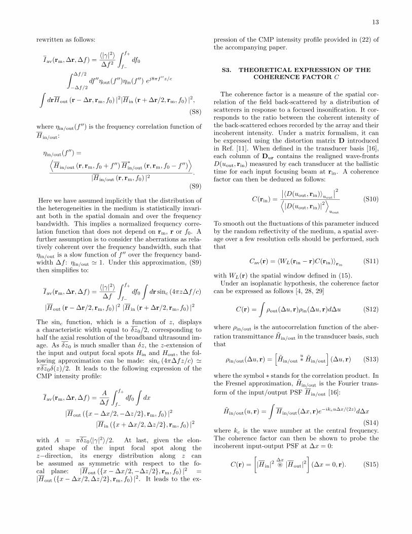
rewritten as follows:

Iav(rm,∆r,∆f) =〈|γ|2〉∆f2

∫ f+

f−

df0∫ ∆f/2

−∆f/2

df ′′ηout(f′′)ηin(f ′′) ej8πf

′′z/c

∫drHout (r−∆r, rm, f0) |2|H in (r + ∆r/2, rm, f0) |2,

(S8)

where ηin/out(f′′) is the frequency correlation function of

H in/out:

ηin/out(f′′) =⟨

H in/out (r, rm, f0 + f ′′)H∗in/out (r, rm, f0 − f ′′)

⟩|H in/out (r, rm, f0) |2

.

(S9)

Here we have assumed implicitly that the distribution ofthe heterogeneities in the medium is statistically invari-ant both in the spatial domain and over the frequencybandwidth. This implies a normalized frequency corre-lation function that does not depend on rm, r or f0. Afurther assumption is to consider the aberrations as rela-tively coherent over the frequency bandwidth, such thatηin/out is a slow function of f ′′ over the frequency band-width ∆f : ηin/out ' 1. Under this approximation, (S9)then simplifies to:

Iav(rm,∆r,∆f) =〈|γ|2〉∆f

∫ f+

f−

df0

∫dr sinc (4πz∆f/c)

|Hout (r−∆r/2, rm, f0) |2 |H in (r + ∆r/2, rm, f0) |2

The sinc function, which is a function of z, displaysa characteristic width equal to δz0/2, corresponding tohalf the axial resolution of the broadband ultrasound im-age. As δz0 is much smaller than δz, the z-extension ofthe input and output focal spots Hin and Hout, the fol-lowing approximation can be made: sinc (4π∆fz/c) 'πδz0δ(z)/2. It leads to the following expression of theCMP intensity profile:

Iav(rm,∆r,∆f) =A

∆f

∫ f+

f−

df0

∫dx

|Hout ({x−∆x/2,−∆z/2}, rm, f0) |2

|H in ({x+ ∆x/2,∆z/2}, rm, f0) |2

with A = πδz0〈|γ|2〉/2. At last, given the elon-gated shape of the input focal spot along thez−direction, its energy distribution along z canbe assumed as symmetric with respect to the fo-cal plane: |Hout ({x−∆x/2,−∆z/2}, rm, f0) |2 =|Hout ({x−∆x/2,∆z/2}, rm, f0) |2. It leads to the ex-

pression of the CMP intensity profile provided in (22) ofthe accompanying paper.

S3. THEORETICAL EXPRESSION OF THECOHERENCE FACTOR C

The coherence factor is a measure of the spatial cor-relation of the field back-scattered by a distribution ofscatterers in response to a focused insonification. It cor-responds to the ratio between the coherent intensity ofthe back-scattered echoes recorded by the array and theirincoherent intensity. Under a matrix formalism, it canbe expressed using the distortion matrix D introducedin Ref. [11]. When defined in the transducer basis [16],each column of Dur contains the realigned wave-frontsD(uout, rin) measured by each transducer at the ballistictime for each input focusing beam at rin. A coherencefactor can then be deduced as follows:

C(rin) =

∣∣〈D(uout, rin)〉uout

∣∣2⟨|D(uout, rin)|2

⟩uout

(S10)

To smooth out the fluctuations of this parameter inducedby the random reflectivity of the medium, a spatial aver-age over a few resolution cells should be performed, suchthat

Cav(r) = 〈WL(rin − r)C(rin)〉rin (S11)

with WL(r) the spatial window defined in (15).Under an isoplanatic hypothesis, the coherence factor

can be expressed as follows [4, 28, 29]

C(r) =

∫ρout(∆u, r)ρin(∆u, r)d∆u (S12)

where ρin/out is the autocorrelation function of the aber-

ration transmittance Hin/out in the transducer basis, suchthat

ρin/out(∆u, r) =[Hin/out

u∗ Hin/out

](∆u, r) (S13)

where the symbol ∗ stands for the correlation product. Inthe Fresnel approximation, Hin/out is the Fourier trans-

form of the input/output PSF H in/out [16]:

Hin/out(u, r) =

∫H in/out(∆x, r)e−ikcu∆x/(2z)d∆x

(S14)where kc is the wave number at the central frequency.The coherence factor can then be shown to probe theincoherent input-output PSF at ∆x = 0:

C(r) =

[|H in|2

∆x~ |Hout|2

](∆x = 0, r). (S15)

14

[1] L. M. Hinkelman, T. L. Szabo, and R. C. Waag, J.Acoust. Soc. Am. 101, 2365 (1997).

[2] F. A. Duck, Physical properties of tissue: A comprehen-sive reference book , 73 (1990).

[3] L. M. Hinkelman, T. D. Mast, L. A. Metlay, and R. C.Waag, J. Acoust. Soc. Am. 104, 3635 (1998).

[4] R. Mallart and M. Fink, J. Acoust. Soc. Am. 96, 3721(1994).

[5] K. W. Hollman, K. W. Rigby, and M. O’Donnell, in 1999IEEE Ultrasonics Symposium. Proceedings. InternationalSymposium, Vol. 2 (1999) pp. 1257–1260.

[6] W. Lambert, L. A. Cobus, M. Couade, M. Fink, andA. Aubry, Phys. Rev. X 10, 021048 (2020).

[7] R. Ali and J. J. Dahl, in 2018 IEEE International Ultra-sonics Symposium (IUS) (IEEE, 2018) pp. 1–4.

[8] M. Jaeger, E. Robinson, H. Gunhan Akarcay, andM. Frenz, Phys. Med. Biol. 60, 4497 (2015).

[9] R. Rau, D. Schweizer, V. Vishnevskiy, and O. Goksel, inIEEE Int. Ultrason. Symp. (IEEE, Glasgow, 2019) pp.2003–2006.

[10] H. Bendjador, T. Deffieux, and M. Tanter, IEEE Trans.Med. Imag. 39, 3100 (2020).

[11] W. Lambert, L. A. Cobus, T. Frappart, M. Fink, andA. Aubry, Proc. Natl. Acad. Sci. USA 117, 14645 (2020).

[12] A. Badon, D. Li, G. Lerosey, A. C. Boccara, M. Fink,and A. Aubry, Sci. Adv. 2, e1600370 (2016).

[13] A. Badon, V. Barolle, K. Irsch, A. Boccara, M. Fink, andA. Aubry, Sci. Adv. 6, eaay7170 (2020).

[14] T. Blondel, J. Chaput, A. Derode, M. Campillo, andA. Aubry, J. Geophys. Res.: Solid Earth 123, 10936(2018).

[15] R. Touma, R. Blondel, A. Derode, M. Campillo, andA. Aubry, arXiv: 2008.01608 (2020).

[16] W. Lambert, L. C. Cobus, M. Fink, and A. Aubry, arXiv:

2103.02036 (2021).[17] A. Aubry and A. Derode, J. Appl. Phys. 106, 044903

(2009).[18] A. Aubry, A. Derode, and F. Padilla, Appl. Phys. Lett.

92, 124101 (2008).[19] G. Montaldo, M. Tanter, J. Bercoff, N. Benech, and

M. Fink, IEEE Trans. Ultrason., Ferroelectr., Freq. Con-trol 56, 489 (2009).

[20] K. Watanabe, Integral transform techniques for Green’sfunctions (Springer, Cham, Switzerland, 2014) Chap. 2.

[21] C. Passmann and H. Ermert, IEEE Trans. Ultrason. Fer-roelectr. Freq. Control 43, 545 (1996).

[22] M.-H. Bae and M.-K. Jeong, IEEE Trans. Ultrason. Fer-roelectr. Freq. Control 47, 1510 (2000).

[23] M. Born and E. Wolf, Principles of optics (Seventh edi-tion) (Cambridge University Press, Cambridge, 2003).

[24] C. Moran, N. Bush, and J. Bamber, Ultrasound MedicineBiol. 21, 1177 (1995).

[25] G. Montaldo, M. Tanter, and M. Fink, Phys. Rev. Lett.106, 054301 (2011).

[26] M. A. Lediju, G. E. Trahey, B. C. Byram, and J. J.Dahl, IEEE Trans. Ultrason. Ferroelectr. Freq. Control58, 1377 (2011).

[27] J. J. Dahl, D. Hyun, Y. Li, M. Jakovljevic, M. A. Bell,W. J. Long, N. Bottenus, V. Kakkad, and G. E. Tra-hey, in 2017 IEEE International Ultrasonics Symposium(IUS) (IEEE, 2017) pp. 1–10.

[28] J.-L. Robert and M. Fink, J. Acoust. Soc. Am. 123, 866(2008).

[29] J.-L. Robert, Evaluation of Green’s functions in complexmedia by decomposition of the Time Reversal Operator:Application to Medical Imaging and aberration correc-tion, Ph.D. thesis, Universite Paris 7 - Denis Diderot(2007).