Ultrahigh Dimensional Feature Screening via RKHS …proceedings.mlr.press/v31/balasubramanian13a.pdf · 126 Ultrahigh Dimensional Feature Screening via RKHS Embeddings Krishnakumar

126

Ultrahigh Dimensional Feature Screening via RKHS Embeddings

Krishnakumar Balasubramanian Bharath K. Sriperumbudur Guy LebanonGeorgia Institute of Technology

[email protected] of [email protected]

Georgia Institute of [email protected]

Abstract

Feature screening is a key step in handling ul-trahigh dimensional data sets that are ubiq-uitous in modern statistical problems. Overthe last decade, convex relaxation based ap-proaches (e.g., Lasso/sparse additive model)have been extensively developed and ana-lyzed for feature selection in high dimensionalregime. But in the ultrahigh dimensionalregime, these approaches suffer from severalproblems, both computationally and statisti-cally. To overcome these issues, in this paper,we propose a novel Hilbert space embeddingbased approach to independence screeningfor ultrahigh dimensional data sets. The pro-posed approach is model-free (i.e., no modelassumption is made between response andpredictors) and could handle non-standard(e.g., graphs) and multivariate outputs di-rectly. We establish the sure screening prop-erty of the proposed approach in the ultra-high dimensional regime, and experimentallydemonstrate its advantages and superiorityover other approaches on several syntheticand real data sets.

1 Introduction

Ultrahigh dimensional data sets are ubiquitous inmodern statistical problems arising from several di-verse scientific fields. For example, several biologi-cal problems or high frequency trading problems haveseveral million features (denoted as p) compared to amuch lesser number of samples (denoted as n). Fea-ture screening plays an important role in analyzingthese ‘large p small n’ data sets. Various penalizationbased techniques that promote sparsity have been de-

Appearing in Proceedings of the 16th International Con-ference on Artificial Intelligence and Statistics (AISTATS)2013, Scottsdale, AZ, USA. Volume 31 of JMLR: W&CP31. Copyright 2013 by the authors.

veloped and analyzed in this regime: Lasso (Tibshi-rani, 1996), Dantzig selector (Candes and Tao, 2007)and scad penalties (Fan and Li, 2001) assume a linearmodel between the covariates and the response, whileSPAM and related techniques (Ravikumar et al., 2009,Huang et al., 2010) assume a non-linear model in orderto select a few relevant features. All these methods al-low for the data dimensionality to be greater than thesample size.

However, there are several issues with the above men-tioned penalty approaches in ultrahigh dimensions.First, these methods cannot efficiently handle ultra-high dimensional settings with p growing faster thana polynomial rate in n, e.g., p growing exponential inn. Secondly, the irrepresentability conditions (Zhaoand Yu, 2007)—these conditions mean that the co-variates not in the true model are not representable, insome sense, by the covariates in the true model—underwhich the model selection consistency is proved for thepenalty methods in high-dimensions, are too stringentto hold in ultrahigh dimensions (see Fan and Lv, 2010,Section 5.5 for general discussion about this and con-crete examples). Thirdly, penalization approaches arecomputationally expensive, e.g., a typical algorithmfor lasso scales as O(p3) with other parameters fixed,hence expensive for ultrahigh dimensional p problems.

In order to tackle this situation, an alternate line of re-search based on marginal regression was proposed andanalyzed (Fan and Lv, 2008, Fan et al., 2009). This isa relatively old technique, that has re-emerged as analternative for feature screening in ultrahigh dimen-sions. The general idea of this approach is to measurethe relationship (to be clearly defined based on con-text) of each feature individually to the response andrank them accordingly. For example, assuming a lin-ear model between response and covariates, Fan andLv (2008) proposed to measure the residual betweenresponse and each covariate (in a least-square sense)and rank the covariates accordingly. In order to relaxthe linear model assumption, Fan et al. (2009) pro-posed screening for generalized linear models based onmarginal utility; Fan et al. (2011) proposed screen-ing using a non-parametric additive model based on

127

Ultrahigh Dimensional Feature Screening via RKHS Embeddings

smoothing splines. Recently, Li et al. (2012) pro-posed a model-free (i.e., without any regressive model-ing assumptions) screening procedure, DC-SIS, basedon distance covariance metric (Szekely et al., 2007)—which is zero if and only if the random variables areindependent—as a measure of relationship between re-sponse and covariate. To elaborate, if the distancecovariance between the response and a covariate is“small”, then the response is independent of the co-variate and therefore such a covariate can be screenedout from consideration. Recently Ji and Jin (2012)showed that a two-step procedure—screening followedby penalized regression—is optimal for feature selec-tion in this regime.

In this paper, we propose a general framework, sup-HSIC-SIS (Hilbert Schmidt independence criterion–Sure independence screening), for model-free, multi-output screening. The approach uses RKHS based in-dependence measures (Gretton et al., 2005) and gener-alizes the previously proposed DC-SIS approach. Thisproposal is motivated from the recent work by Se-jdinovic et al. (2012a) who established the equiva-lence between distance covariance and HSIC (a de-pendence/independence measure based on RKHS em-bedding of probabilities). Given this equivalence, it isstraight forward to propose an independence screeningprocedure based on HSIC by replacing distance covari-ance in (Li et al., 2012) with HSIC and carrying outthe analysis verbatim. However, a major issue withDC-SIS (or its equivalent RKHS version, say HSIC-SIS) is that the employed independence measure isjust one member of a parametric family of indepen-dence measures and there is no guarantee that thismember provides the best screening procedure over allthe other choices from this family. In other words, ifwe consider HSIC-SIS, the choice of kernel determinesthe performance of the screening procedure.

Our main contribution in this paper is to address thisissue by using an independence measure (that adaptsto the joint distribution between the response and co-variates) that is obtained by taking the supremum ofHSIC over a family of kernels, and theoretically showthat sup-HSIC-SIS enjoys the sure screening propertyunder some regularity conditions. Furthermore, wepropose two iterative versions of sup-HSIC-SIS thataddress issues inherent in any marginal screening pro-cedure and are robust to the assumed regularity con-ditions. We empirically show that these proposed ex-tensions along with sup-HSIC-SIS perform better thanthe existing approaches, while the theoretical analysisof these extensions are left out for future work.

A related RKHS based approach was previously pro-posed for feature selection in Song et al. (2012). Theapproach uses HSIC metric and deals primarily withthe low-dimensional setting (i.e., n > p) and is ba-

sically a model-free version of subset selection ap-proaches used in linear regression settings. Comparingtheir empirical results with ours (see Sections 6.4 and6.5), we note that while BA-HSIC is suitable for low-dimensions and to some extent for high-dimensionalsettings, it does not perform well in ultrahigh dimen-sional settings. In addition, while (Song et al., 2012)do not provide any theoretical guarantees for their ap-proach, we conjecture that BA-HSIC performs inferiorto DC-SIS and sup-HSIC-SIS in ultrahigh dimensionalsettings using the arguments similar to the ones usedin (Li et al., 2012).

The paper is organized as follows. In Section 2, weintroduce the sup-HSIC dependence measure. In Sec-tion 3, we discuss how it could be used for featurescreening in ultra-high dimensions. The sure screeningproperty of sup-HSIC-SIS is then analyzed in Section 4and two related iterative extensions are discussed inSection 5. Experimental results comparing the pro-posed methods with various other approaches on syn-thetic and real-world data sets are provided in Sec-tion 6. Missing proofs are provided in an appendix.

2 RKHS embedding of probabilities

Recently, the notion of embedding probability mea-sures into a reproducing kernel Hilbert space (RKHS)has been proposed as a generalization to the classicalkernel method (which embeds points from an inputspace into an RKHS) with a motivation to provide alinear method for handling higher-order statistics ofrandom variables (Berlinet and Thomas-Agnan, 2004,Smola et al., 2007). This notion has gained popularityin various applications including hypothesis testing,dimensionality reduction and reinforcement learning(see Nishiyama et al., 2012, and references therein).Formally, given a Borel probability measure, P definedon a topological space, X , and the RKHS (H, k) offunctions on X with bounded and measurable k asits reproducing kernel, the embedding of P into H isdefined as Pk :=

∫X k(·, x) dP(x). Given two Borel

probability measures, P and Q, Gretton et al. (2007)defined the RKHS distance between their embeddingsas the maximum mean discrepancy (MMD), i.e.,

γk(P,Q)def=

∥∥∥∥∫Xk(·, x) dP(x)−

∫Xk(·, x) dQ(x)

∥∥∥∥H.

Note that when the kernel k is characteristic (Sripe-rumbudur et al., 2010), the embeddings are injective,i.e., γk(P,Q) = 0 if and only if P = Q and thusγk defines a metric on the space of probability mea-sures. One of the applications of the above metric isin capturing the degree of dependence between tworandom variables X ∈ X and Y ∈ Y with marginaldistributions PX and PY and jointly distributed asPXY . Assuming k : (X × Y)2 → R to be separa-

128

Krishnakumar Balasubramanian, Bharath K. Sriperumbudur, Guy Lebanon

ble, i.e., k((x, y), (x′, y′)) = kX (x, x′)kY(y, y′), wherekX : X 2 → R and kY : Y2 → R are reproducing kernelsof HX and HY respectively (so that H ∼= HX ⊗HY),γ2k reduces to the Hilbert-Schmidt independence crite-rion (Gretton et al., 2005) between X and Y , definedas

γ2k(PXY ,PXPY )def= ‖PXY k − PXPY k‖2H

= EXX′Y Y ′ [kX (X,X ′)kY(Y, Y ′)]

+EXX′ [kX (X,X ′)]E Y Y ′ [kY(Y, Y ′)]

−2EXY [EX′ [kX (X,X ′)]E Y ′ [kY(Y, Y ′)]] , (1)

where X ′ and Y ′ are independent copies of X andY respectively. Gretton et al. (2005) showed thatγk(PXY ,PXPY ) is the Hilbert-Schmidt norm of thecross-covariance operator between HX and HY , withthe property that when kX and kY are characteristic:γk(PXY ,PXPY ) is zero iff X and Y are independent.This crucial property of γk will be exploited later inour screening framework. A drawback of the abovemetric is: typically the kernel comes with a tuningparameter that should be selected in practice usingheuristics. In order to deal with this problem, Sripe-rumbudur et al. (2009) proposed the following mod-ification (actually proposed in the context of MMD,which we here present in the context of HSIC) whichwe call as sup-HSIC:

γ(PXY ,PXPY )def= sup{γk(PXY ,PXPY ) : k ∈ K}.

Note that γ represents the maximal distance betweenPXY and PXPY over the family of kernels K. If anyk ∈ K is characteristic, then γ is a metric. Typi-cal example includes the family of Gaussian kernels

KG(u, v) when kX = kYdef= {exp−σ‖u−v‖

22 : σ ∈ R+}.

See (Sriperumbudur et al., 2009) for more details andexamples.

In statistical problems, we are given n random samples{(x(1), y(1)), . . . , (x(n), y(n))} drawn i.i.d. from PXY .Given these samples, an estimate γ of sup-HSIC isdefined as:

γ(PXY ,PXPY )def= sup{‖PXYn k − PXn PYn k‖H : k ∈ K},

=1

nsup

kX∈KX ,kY∈KY

√trace (KXH KYH)

where PXYn ,PXn and PYn represent the empirical mea-sures over the given samples, KX and KY are n × nGram matrices associated with kX and kY respectively,H = I− 1

n11> where I is n× n identity matrix and 1is a n× 1 vector of ones.

3 Screening via RKHS embedding

In this section, we describe how the sup-HSIC measureof independence could be used for feature screening

in ultrahigh dimensions. We assume a response Y ∈Rd and covariates X ∈ Rpn , with pn growing withn and d fixed (for simplicity). The method appliesas well to more general topological spaces X ,Y. Weuse Xr to denote the r-component of X and XS todenote the components of X indexed by the elementsof the set S. We denote the n training set samplesas {(x(1), y(1)), . . . , (x(n), y(n))} where n can be verysmall compared to pn. Under such an assumption, itis natural to assume that only a subset of covariatesare related to the response Y .

Following Li et al. (2012), we define the set of relevantvariables M and irrelevant variables I as:

M = {r : P(Y |X) depends on Xr}I = {r : P(Y |X) does not depend on Xr}

where P(Y |X) is the conditional distribution of Ygiven X. Note that given XM, XI is conditionallyindependent of Y and hence redundant while calculat-ing the response. With this definition, feature selec-tion involves estimating the set M from the given nsamples.

A natural idea is to rank the covariates according totheir degree of dependence to the response. In order tomeasure such a degree of dependence of the dimensionXr to Y , we use the sup-HSIC measure introducedin the previous section. Specifically, we use the sup-HSIC between the joint random variable (Xr, Y ) andthe marginals Xr and Y . Denoting the joint distribu-tion of the vector (Xr, Y ) as PXrY and the marginaldistribution of the dimensions Xr and Y as PXr andPY respectively, we define

ωrdef= γr(PXrY ,PXrPY )

to be the measure of dependence between the rth di-mension Xr and the response Y . Note that γr = 0 iffXr is independent of Y and greater the value, greaterthe degree of dependence. These properties make sup-HSIC suitable for ranking the dimensions of X ac-cording to the degree of dependence to the responseY . In practice, given n samples, we use the empiricalestimator γ defined in the previous section. Specifi-cally, we denote the corresponding empirical estimateas ωr = γr(PXrY

n ,PXrn PYn ).

In order to select the relevant variables (i.e., to esti-mate M), we first compute ωr for r = 1, . . . , pn anddefine

M = {r : ωr ≥ cn−κ, for 1 ≤ r ≤ pn}

where 0 ≤ κ < 1/2, as the estimated set of relevantfeatures. Note that the set of relevant features is de-fined as the set of all dimensions that have dependencegreater than cn−κ with the response. The thresholddefined here depends on the value of n. When n is

129

Ultrahigh Dimensional Feature Screening via RKHS Embeddings

large, naturally it allows for variables with weaker de-pendence to be detected.

The approach above has several nice properties. First,the method is model free as it does not assume a spe-cific regression model between X and Y . Second, theresponse Y may be a vector or more generally a graphor a ranking. As a result, the method can be usedfor feature selection in the case of multi-label classifi-cation and multivariate output regression. Third, themethod chooses the kernel k in a principled way by se-lecting k from a family of positive definite kernels thatmaximizes the Hilbert Schmidt norm of the covarianceoperator. Finally, as we show in the next section themethod generalizes the recently proposed DC-SIS (Liet al., 2012).

3.1 DC-SIS as a special case of sup-HSIC-SIS

In order to see how the proposed method generalizesthe recent approach by Li et al. (2012), we appeal tothe general equivalence between distance based inde-pendence metrics and kernel based independence met-rics, as established by Sejdinovic et al. (2012a). Tosummarize DC-SIS briefly, Li et al. (2012) uses dis-tance covariance metric (Szekely et al., 2007) as a mea-sure of independence in the screening approach. In or-der to see the connection, we first need the followingdefinition due to Lyons (2012).

Definition 1. Let (X , ρX ) and (Y, ρY) be semi-metricspaces of negative type (cf. Lyons (2012)), with ran-dom variables X and Y taking values in X and Y re-spectively. The distance covariance between X and Yis defined as

dcov2(X,Y ) = EX,Y EX′,Y ′ρX (X,X ′)ρY(Y, Y ′)

+ EXEX′ρX (X,X ′)E Y ,E Y ′ρX (X,X ′)

− 2EX,Y (EX′ρX (X,X ′)E Y ′ρX (X,X ′)) .

When X = Rs and Y = Rt with ρX = ρY = ‖ · − · ‖,dcov reduces to the distance used in (Szekely et al.,2007). The following result due to Sejdinovic et al.(2012b) establishes the equivalence between dcov andγk.

Theorem 3.1. Let (X , ρX ) and (Y, ρY) be semi-metric spaces of negative type with X ∼ PX andY ∼ PY having joint PXY . Let kX and kY be ker-nels on X and Y that generate the respective met-rics and denote k((x, y), (x′, y′)) = kX (x, x′)kY(y, y′).Then dcov2(X,Y ) = 4γ2k(PXY ,PXPY ).

Example 11 in (Sejdinovic et al., 2012b) shows thatkq(x, x

′) = 12 (‖x‖q+‖x′‖q−‖x−x′‖q), x, x′ ∈ Rd, 0 <

q ≤ 2 generates a semi-metric, ρq(x, x′) = ‖x−x′‖q of

negative type. Choosing kX = kY = k1 yields the dcovmetric as proposed in (Szekely et al., 2007), which isused in DC-SIS. But there is no reason to fix q = 1 and

it is not possible to know appropriate q a priori, whichmotivates the use of sup-HSIC as a dependence mea-sure in sup-HSIC-SIS, thereby generalizing DC-SIS. Inaddition, the proposed generalization enables one towork with a wide variety of kernel families (and notjust {kq : 0 < q ≤ 2}) and provides a richer set of inde-pendence measures between random variables, whichin turn enables one to do better model-free feature se-lection. Thus the proposed sup-HSIC-SIS procedureis strictly more general than the DC-SIS method, andachieves better empirical results as demonstrated inSection 6.

4 Theoretical analysis

In this section, we prove the sure screening propertyof sup-HSIC-SIS for X ⊂ Rpn and Y ⊂ Rd. Our anal-ysis applies to a range of kernel families and does notimpose any moment conditions on the variables X andY . Further it provides a simpler proof under relaxedassumption compared to Li et al. (2012) even for DC-SIS. For simplicity, we let d to be fixed, but one couldalso analyze the dependency on d to determine thejoint scaling of d and pn with n. We allow the cardi-nality of the active set to scale with n, i.e., |Mn| = sn.The main assumptions we impose are the following:

A1 sup{kX (x, x) : kX ∈ KX , x ∈ X} = A <∞A2 sup{kY(y, y) : kY ∈ KY , y ∈ Y} = A <∞A3 min

r∈Mωr ≥ 2cn−κ for some c > 0 and κ ∈ [0, 1/2).

Assumption A3 requires that sup-HSIC measure cor-responding to the relevant variables cannot be toosmall, which is similar to condition 3 of Fan and Lv(2008) and various other previous works that analyzedmarginal screening approaches. The proof of surescreening property of sup-HSIC-SIS in Theorem 4.1,uses an intermediate result in Lemma 1 (stated andproved in the appendix).

Definition 2. Let G be a class of functions on X ×Xand {ρ1, . . . ρn} be independent Rademacher randomvariables. The homogeneous Rademacher chaos pro-cess of order two with respect to {ρ1, . . . ρn} is de-fined as {n−1

∑ni<j ρiρjg(xi, xj) : g ∈ G} for some

{x1, . . . , xn} ⊂ X . The Rademacher chaos complexityof G is defined as

Un(G; {xi})def= E ρ sup

g∈G

∣∣∣∣∣∣ 1nn∑i<j

ρiρjg(xi, xj)

∣∣∣∣∣∣ .Theorem 4.1. Let kX and kY be measurable ker-nels satisfying assumptions A1 and A2. Define D :={(x(i), y(i))}ni=1. Then we have

(PXY )n({

D ∈ (X × Y)n : max1≤r≤pn

|ωr − ωr| ≥ cn−κ)}

≤ 6pn exp

(−(cn

12−k−Rn−6A

)2

162A2

),(2)

130

Krishnakumar Balasubramanian, Bharath K. Sriperumbudur, Guy Lebanon

where Rndef=√

8AUn(KY ; {y(i)}) +

supr

(√8Un(K; {(x(i)r , y(i))}) +

√8AUn(KX ; {x(i)r })

).

Furthermore if assumption A3 is also satisfied, thenwe have the following sure screening property:

(PXY )n(M⊆ M

)≥ 1−O

sne−(cn

12−k−Rn−6A

)2

162A2

.

Proof. The proof of (2) follows from applying Lemma1 from the appendix for each r followed by a unionbound. In order to prove the sure screening prop-

erty, if M * M, then there must exist some r ∈ Msuch that ωr < cn−κ. But, from the assumption A3,we have that |ωr − ωr| > cn−κ for some r ∈ M.

Hence we note that the event {M * M} happensif {|ωr−ωr| > cn−κ}, for some r ∈M. Define Γ to bethe event {maxr∈M |ωr − ωr| ≤ cn−κ}. Then we have

(PXY )n(M⊆ M

)≥ (PXY )n(Γ) and the following se-

quence of inequality holds. Define Prdef= (PXY )n.

Pr(Γ)=1− Pr(Γc) = 1− Pr

(minr∈M

|ωr − ωr| ≥ cn−κ)

=1− snPr(|ωr − ωr| ≥ cn−κ

)≥1−O

(sn exp

(−(cn−κ+1/2 − Rn − 6A

)2162A2

)).

This completes the proof.

Note that an important quantity controlling the ratesis the term Rn that involves the Rademacher chaoscomplexities of K, KX and KY . Sriperumbudur et al.(2009) has shown that for VC-subgraph classes of ker-nels, the Rademacher chaos complexity is boundedabove by a constant that depends on the VC dimen-sion of the class. Examples of such kernel classesin a d-dimensional Euclidean space include Gaus-sian, Laplacian, Matern class etc. We refer thereader to (Sriperumbudur et al., 2009) for a de-tailed discussion and several more examples. Inour setting, if K, KX and KY are VC subgraphclasses, then Pr (max1≤r≤pn |ωr − ωr| ≥ cn−κ) ≤O(pn exp(−c1n1−2κ)

)from which we observe that the

proposed approach enables us to handle ultrahigh di-mensionality, i.e., log pn = o(n1−2κ).

In order to control the false positive rates, if we assumethat maxr/∈M |ωr| = O(n−κ), then with probabilitytending to 1, we have

maxr/∈M

|ωr| ≤ C(n−κ).

for some constant C > 0. By applying Theorem 4.1,

we have: Pr(M = M) = 1−O(1). This gives a model

selection consistency result under the assumption thatthere is a strict separation between the set of relevantand irrelevant variables. But to be more general, we

analyze below, the cardinality of the set M.

4.1 Upper bounding the cardinality of M

A main reason for performing feature screening is toreduce the dimensionality from exponential to some-thing that could be handled, say polynomial with thesample size. With that one could use cleaning proce-dures to further refine the feature selection process. Inthis section, we show that by appropriately selectingthe bound on the kernel (i.e., the value A), one couldmake the cardinality of the estimated set grow poly-nomially in the sample size. Specifically, we have thefollowing theorem.

Theorem 4.2. Let kX and kY be measurable kernelssatisfying assumptions A1 and A2. Then there existsa constant c > 0 such that,

(PXY )n(|M| ≤ O(nκpnA)

)≥ 1− pne−

(cn

12−k−Rn−6A

)2

162A2 .

Proof. First we note that∑pnr=1 ωr ≤ pn maxr ωr ≤

CApn = O(Apn). Now this would imply that |{r :ωr > εn−κ}| cannot exceed O(nκApn) for any ε > 0.Thus on the set, Υ = {max1≤r≤d |ωr − ωr| ≤ εn−κ},|{r : ωr > 2εn−κ}| cannot exceed |{r : ωr > εn−κ}|,which would be bounded by O(nκApn). If we take

ε = c/2, we have Pr(|M| ≤ O(nκAp)) ≥ Pr(Υ) andthe conclusion follows from (2).

The main consequence of the above theorem is thatwhen A = O(nτ/pn), for some τ > 0, then we have

|M| = O(nκ+τ ) and thus the size of the selected set isof polynomial order in n. Compared to the initial casewhen the dimensionality is of exponential order, thisis a huge improvement in terms of feature selection.This also gives us some insights on how to design orselect kernels such that we could have a control overthe cardinality of the selected feature set size.

5 Iterative Screening procedures

Any screening method based on marginal computa-tions suffers from the following problems (cf. (Fanet al., 2009)): (1) any irrelevant covariate that is highlycorrelated with the set of relevant covariates could beselected and (2) marginally uncorrelated covariate thatis jointly correlated with the response might not be se-lected. Here, we propose two approaches that could beused in order to handle such scenarios.

131

Ultrahigh Dimensional Feature Screening via RKHS Embeddings

5.1 Method 1

We first consider the situation when important covari-ates are marginally weakly correlated, but jointly cor-related to the response. In order to deal with thissituation, we propose the following iterative method:

1. Compute sup-HSIC between each dimension andresponse and select the covariates that have ωr >

λt. Let M(t) be the set of selected covariates atround t with XM(t)

being the set of selected fea-

tures.

2. Compute sup-HSIC between (Y, (XM(t), Xj)) and

marginal Y and (XM(t), Xj)) for all j ∈ Mc

(t).

The selected feature set M′(t) consists of covari-

ates j for which the above calculated sup-HSICis greater than the sup-HSIC between (Y,XM(t)

)

and the marginal Y and XM(t). Update M(t) =

M(t−1) ∪ M′(t)3. Repeat the procedure till M(t) = M(t−1) or until

|⋃t M(t)| > n.

In the above iterative approach, the threshold λt isset at a high value during the initial rounds and re-duced as the rounds progress. In practice, it couldbe selected using cross-validation. Heuristics for se-lecting the threshold for such iterative methods couldbe found in (Fan et al., 2009). The above iterativeapproach would be able to detect covariates that aremarginally uncorrelated with the response (and hencenot selected in initial rounds), but are jointly corre-lated because we measure sup-HSIC between the jointvector (XM(t)

, Xj) and the response Y .

5.2 Method 2

This approach is motivated by the iterative screeningprocedure proposed by Fan and Lv (2008) which wasbased on residuals computed between the covariatesand response under a linear model assumption. It isnot possible to directly adopt such a procedure in ourcase, as the proposed approach is model-free. In or-der to proceed, first we introduce the input residual

matrix. Let XM(t)∈ Rn×|M(t)| be data matrix associ-

ated with selected covariates at round t and XMc(t)

∈

Rn×(p−|M(t)|) be data matrix corresponding to the re-maining covariates. The input residual matrix is de-fined as the projection of complement of selected vari-ables in a particular step onto the orthogonal comple-ment space of the selected variables in that step, i.e.,X(t)r = {In×n −XM(t)

(X>M(t)XM(t)

)−1X>M(t)}XMc

(t)

.

The key idea of this approach is that the input resid-ual matrix at a particular step is uncorrelated with thespace of selected variables in that step. Thus covari-ates that would have been selected because they are

correlated with a true relevant covariate (and hencecorrelated with the response) could be avoided in thisapproach. This discussion leads to the following ap-proach:

1. Calculate sup-HSIC to the original data set and

let M(t) be set of selected features at round t.

2. Compute the residual data matrix, X(t)r =

{In×n−XM(t)(X>M(t)

XM(t))−1X>M(t)

}XMc(t)

and

compute sup-HSIC between X(t)r and the response

to obtain the selected feature set M′(t) and up-

date M(t) = M(t−1) ∪ M′(t). Stop when M(t) =M(t−1) or |

⋃t M(t)| > n.

Similar to Method 1, the threshold for the initialrounds are set at high value and subsequently low-ered. Since the residual matrix at each step is notcorrelated with the selected covariates, the covariatesthat are strongly correlated with any of true active co-variates would not be selected. Also covariates thatwere actually correlated to the response (but were notselected) would now be detected easily.

6 Experiments

In this section, we report experimental results on vari-ous synthetic and real-world data sets to demonstratethe advantage of the proposed approach (sup-HSIC-SIS) over various feature screening approaches. Forthe experiments on synthetic data, we consider datasettings from (Li et al., 2012) in order to make a directcomparison to their approach. For evaluation on real-world data, we consider a very high dimensional genedata set and a multi-label data set and show that theproposed approach performs significantly better thanthe existing approaches.

6.1 Synthetic data – univariate response

The synthetic data set is generated as follows: X ∼N(0,Σ) where Σ ∈ Rp×p with entries σi,j = 0.8|i−j|.We set n = 200 and let p to be 5000. We generate theresponse Y according to three models:

1. Y = c1β1X1X2 + c3β21(X12 < 0) + c4β3X22 + ε

2. Y = c1β1X1X2 + c3β21(X12 < 0)X22 + ε

3. Y = c1β1X1 + c2β2X2 + c3β31(X12 < 0) +exp(c4|X22||)ε

where βj = (−1)U (a + |Z|) where a = 4 log n/√n,

U ∼ Bernoulli(0.4) and Z, ε ∼ N(0.1). Note that allmodels are non-linear in X12. Further the third modelis heteroscedastic. For the fourth data set, the rela-tionship between the response and covariates is givenby the following joint model, PXrY ∝ 1+sin(lx) sin(ly)for integer l, on the support [−π, π]× [−π, π] for eachr. Note that when l = 0, Xr and Y are independent

132

Krishnakumar Balasubramanian, Bharath K. Sriperumbudur, Guy Lebanon

NIS q = 1 q = 12 q = 1

4 supq kq Gauss.

P (M∗ = M)0.78 0.79 0.82 0.84 0.88 0.870.73 0.75 0.79 0.80 0.83 0.840.73 0.73 0.75 0.78 0.82 0.820.35 0.40 0.52 0.60 0.71 0.80

P (M∗ ⊂ M)0.96 0.98 1.00 1.00 1.00 1.000.94 0.95 0.99 1.00 1.00 1.000.93 0.96 1.00 1.00 1.00 1.000.6 0.69 0 .72 0.75 0.92 0.98

|M|10.1 7.4 5.4 4.4 4.2 4.2

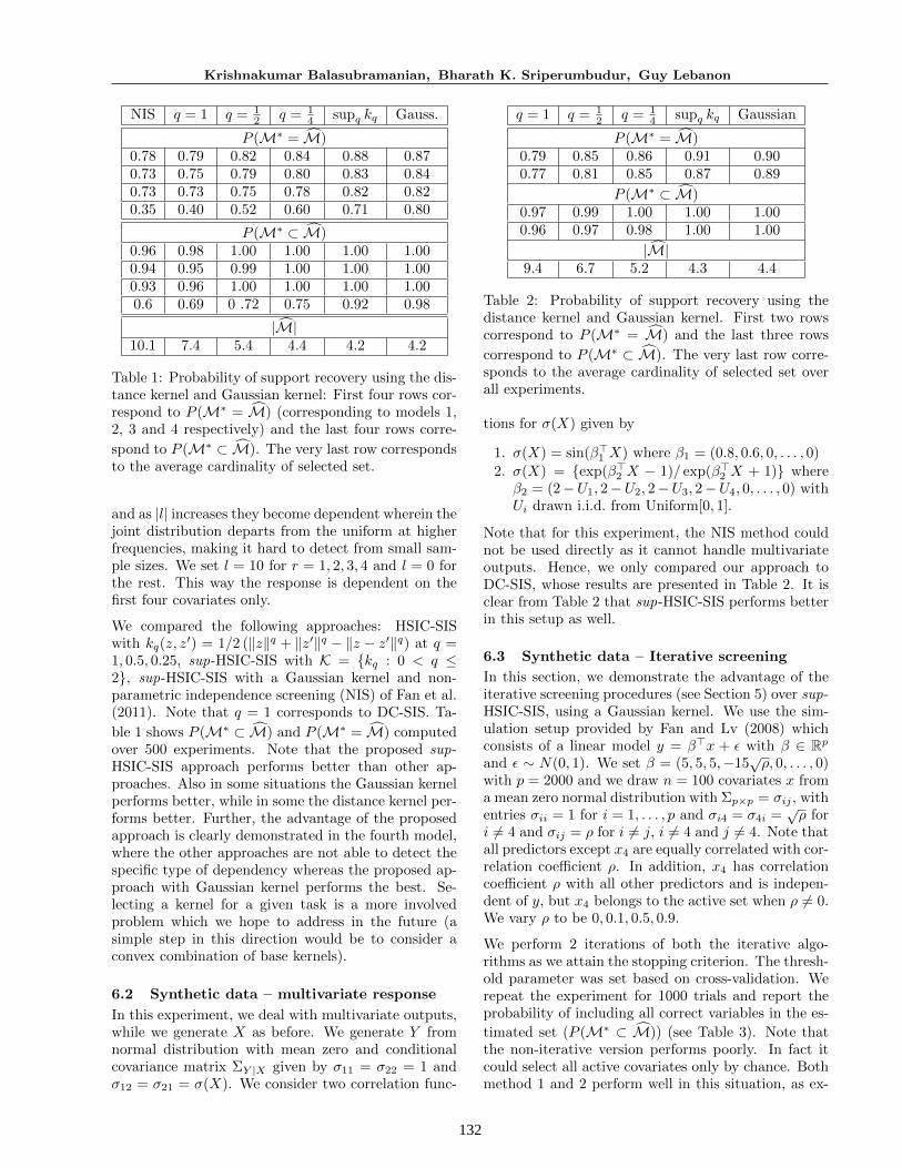
Table 1: Probability of support recovery using the dis-tance kernel and Gaussian kernel: First four rows cor-respond to P (M∗ = M) (corresponding to models 1,2, 3 and 4 respectively) and the last four rows corre-

spond to P (M∗ ⊂ M). The very last row correspondsto the average cardinality of selected set.

and as |l| increases they become dependent wherein thejoint distribution departs from the uniform at higherfrequencies, making it hard to detect from small sam-ple sizes. We set l = 10 for r = 1, 2, 3, 4 and l = 0 forthe rest. This way the response is dependent on thefirst four covariates only.

We compared the following approaches: HSIC-SISwith kq(z, z

′) = 1/2 (‖z‖q + ‖z′‖q − ‖z − z′‖q) at q =1, 0.5, 0.25, sup-HSIC-SIS with K = {kq : 0 < q ≤2}, sup-HSIC-SIS with a Gaussian kernel and non-parametric independence screening (NIS) of Fan et al.(2011). Note that q = 1 corresponds to DC-SIS. Ta-

ble 1 shows P (M∗ ⊂ M) and P (M∗ = M) computedover 500 experiments. Note that the proposed sup-HSIC-SIS approach performs better than other ap-proaches. Also in some situations the Gaussian kernelperforms better, while in some the distance kernel per-forms better. Further, the advantage of the proposedapproach is clearly demonstrated in the fourth model,where the other approaches are not able to detect thespecific type of dependency whereas the proposed ap-proach with Gaussian kernel performs the best. Se-lecting a kernel for a given task is a more involvedproblem which we hope to address in the future (asimple step in this direction would be to consider aconvex combination of base kernels).

6.2 Synthetic data – multivariate response

In this experiment, we deal with multivariate outputs,while we generate X as before. We generate Y fromnormal distribution with mean zero and conditionalcovariance matrix ΣY |X given by σ11 = σ22 = 1 andσ12 = σ21 = σ(X). We consider two correlation func-

q = 1 q = 12 q = 1

4 supq kq Gaussian

P (M∗ = M)0.79 0.85 0.86 0.91 0.900.77 0.81 0.85 0.87 0.89

P (M∗ ⊂ M)0.97 0.99 1.00 1.00 1.000.96 0.97 0.98 1.00 1.00

|M|9.4 6.7 5.2 4.3 4.4

Table 2: Probability of support recovery using thedistance kernel and Gaussian kernel. First two rowscorrespond to P (M∗ = M) and the last three rows

correspond to P (M∗ ⊂ M). The very last row corre-sponds to the average cardinality of selected set overall experiments.

tions for σ(X) given by

1. σ(X) = sin(β>1 X) where β1 = (0.8, 0.6, 0, . . . , 0)

2. σ(X) = {exp(β>2 X − 1)/ exp(β>2 X + 1)} whereβ2 = (2−U1, 2−U2, 2−U3, 2−U4, 0, . . . , 0) withUi drawn i.i.d. from Uniform[0, 1].

Note that for this experiment, the NIS method couldnot be used directly as it cannot handle multivariateoutputs. Hence, we only compared our approach toDC-SIS, whose results are presented in Table 2. It isclear from Table 2 that sup-HSIC-SIS performs betterin this setup as well.

6.3 Synthetic data – Iterative screening

In this section, we demonstrate the advantage of theiterative screening procedures (see Section 5) over sup-HSIC-SIS, using a Gaussian kernel. We use the sim-ulation setup provided by Fan and Lv (2008) whichconsists of a linear model y = β>x + ε with β ∈ Rpand ε ∼ N(0, 1). We set β = (5, 5, 5,−15

√ρ, 0, . . . , 0)

with p = 2000 and we draw n = 100 covariates x froma mean zero normal distribution with Σp×p = σij , withentries σii = 1 for i = 1, . . . , p and σi4 = σ4i =

√ρ for

i 6= 4 and σij = ρ for i 6= j, i 6= 4 and j 6= 4. Note thatall predictors except x4 are equally correlated with cor-relation coefficient ρ. In addition, x4 has correlationcoefficient ρ with all other predictors and is indepen-dent of y, but x4 belongs to the active set when ρ 6= 0.We vary ρ to be 0, 0.1, 0.5, 0.9.

We perform 2 iterations of both the iterative algo-rithms as we attain the stopping criterion. The thresh-old parameter was set based on cross-validation. Werepeat the experiment for 1000 trials and report theprobability of including all correct variables in the es-

timated set (P (M∗ ⊂ M)) (see Table 3). Note thatthe non-iterative version performs poorly. In fact itcould select all active covariates only by chance. Bothmethod 1 and 2 perform well in this situation, as ex-

133

Ultrahigh Dimensional Feature Screening via RKHS Embeddings

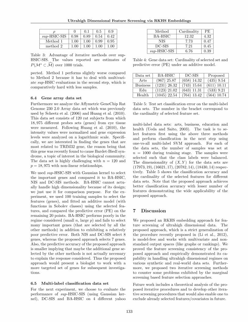
ρ 0 0.1 0.5 0.9sup-HSIC-SIS 0.98 0.89 0.54 0.42

Method 1 1.00 1.00 0.99 0.95method 2 1.00 1.00 1.00 1.00

Table 3: Advantage of iterative methods over sup-HSIC-SIS. The values reported are estimates of

P (M∗ ⊂ M) over 1000 trials.

pected. Method 1 performs slightly worse comparedto Method 2 because it has to deal with multivari-ate sup-HSIC evaluations in the second step, which iscomparatively hard with less samples.

6.4 Gene array data set

Furthermore we analyze the Affymetric GeneChip RatGenome 230 2.0 Array data set which was previouslyused by Scheetz et al. (2006) and Huang et al. (2010).This data set consists of 120 rat subjects from which18, 975 different probes sets (genes) from eye tissuewere measured. Following Huang et al. (2010), theintensity values were normalized and gene expressionlevels were analyzed on a logarithmic scale. Specifi-cally, we are interested in finding the genes that aremost related to TRIM32 gene, the reason being thatthis gene was recently found to cause Bardet-Biedl syn-drome, a topic of interest in the biological community.The data set is highly challenging with n = 120 andp = 18, 975 with non-linear relationships.

We used sup-HSIC-SIS with Gaussian kernel to selectthe important genes and compared it to BA-HSIC,NIS and DC-SIS methods. BA-HSIC cannot actu-ally handle high dimensionality because of its design;we just use it for comparison purpose. For the ex-periment, we used 100 training samples to select thefeatures (genes), and fitted an additive model (withfunctions in Sobolev classes) using the selected fea-tures, and compared the predictive error (PE) on theremaining 20 points. BA-HSIC performs poorly in theregime considered (small n, large p) and fails to selectmany important genes (that are selected by all theother methods) in addition to exhibiting a relativelypoor predictive error. Both NIS and DC-SIS select 8genes, whereas the proposed approach selects 7 genes.Also, the predictive accuracy of the proposed approachis smaller implying that maybe the additional gene se-lected by the other methods is not actually necessaryto explain the response considered. Thus the proposedapproach would present a biologist to work with amore targeted set of genes for subsequent investiga-tions.

6.5 Multi-label classification data set

For the next experiment, we choose to evaluate theperformance of sup-HSIC-SIS (using Gaussian ker-nel), DC-SIS and BA-HSIC on 4 different yahoo

Method Cardinality PEBA-HSIC 12.32 4.32

NIS 7.73 0.47DC-SIS 7.21 0.45

sup-HSIC-SIS 6.76 0.39

Table 4: Gene data set: Cardinality of selected set andpredictive error (PE) under an additive model.

Data set BA-HSIC DC-SIS ProposedArts (967) 25.87 (658) 14.32 (435) 9.54

Business (1231) 26.32 (743) 15.64 (611) 10.11Edu (1123) 21.02 (643) 11.31 (533) 9.21

Health (1045) 22.54 (764) 13.42 (564) 10.74

Table 5: Test set classification error on the multi-labeldata sets. The number in the bracket correspond tothe cardinality of selected feature set.

multi-label data sets: arts, business, education andhealth (Ueda and Saito, 2003). The task is to se-lect features first using the above three methodsand perform classification in the next step usingone-vs-all multi-label SVM approach. For each ofthe data sets, the number of samples was set atn = 1000 during training stage. The samples wereselected such that the class labels were balanced.The dimensionality of (X,Y ) for the data sets are(17973, 19), (16621, 17), (20782, 14), (18430, 14) respec-tively. Table 5 shows the classification accuracy andthe cardinality of the selected features for differentdata sets. Note that the proposed approach achievesbetter classification accuracy with lesser number offeatures demonstrating the wide applicability of theproposed approach.

7 Discussion

We proposed an RKHS embedding approach for fea-ture screening of ultrahigh dimensional data. Theproposed approach, which is a strict generalization ofthe procedure recently proposed in (Li et al., 2012),is model-free and works with multivariate and non-standard output spaces (like graphs or rankings). Weproved the feature screening consistency of the pro-posed approach and empirically demonstrated its ca-pability in handling ultrahigh dimensional regimes onvarious synthetic and real-world data sets. Further-more, we proposed two iterative screening methodsto counter some problems exhibited by the marginalscreening based feature selection approaches.

Future work includes a theoretical analysis of the pro-posed iterative procedures and to develop other itera-tive screening procedures that would also enable one toexclude already selected features/covariates in future.

134

Krishnakumar Balasubramanian, Bharath K. Sriperumbudur, Guy Lebanon

References

Berlinet, A. and Thomas-Agnan, C. (2004). Reproduc-ing Kernel Hilbert Spaces in Probability and Statis-tics. Kluwer Academic Publishers, London, UK.

Candes, E. and Tao, T. (2007). The Dantzig selector:Statistical estimation when p is much larger than n.Annals of Statistics, 35(6):2313–2351.

Fan, J., Feng, Y., and Song, R. (2011). Nonpara-metric independence screening in sparse ultra-high-dimensional additive models. J. Amer. Statist. As-soc., 106(494):544–557.

Fan, J. and Li, R. (2001). Variable selection via non-concave penalized likelihood and its oracle proper-ties. J. Amer. Statist. Assoc., 96(456):1348–1360.

Fan, J. and Lv, J. (2008). Sure independence screen-ing for ultrahigh dimensional feature space. J. Roy.Statist. Soc. Ser. B, 70:849–911.

Fan, J. and Lv, J. (2010). A selective overview ofvariable selection in high dimensional feature space.Statistica Sinica, 20:101–148.

Fan, J., Samworth, R., and Wu, Y. (2009). Ultrahighdimensional feature selection: Beyond the linearmodel. J. of Machine Learning Research, 10:2013–2038.

Gretton, A., Borgwardt, K. M., Rasch, M., Scholkopf,B., and Smola, A. (2007). A kernel method for thetwo sample problem. In Advances in Neural Infor-mation Processing Systems 19, pages 513–520.

Gretton, A., Bousquet, O., Smola, A., and Scholkopf,B. (2005). Measuring statistical dependence withHilbert-Schmidt norms. In Proc. of the 16th Inter-national Conference on Algorithmic Learning The-ory, pages 63–77.

Huang, J., Horowitz, J., and Wei, F. (2010). Variableselection in nonparametric additive models. Annalsof statistics, 38(4):2282–2313.

Ji, P. and Jin, J. (2012). UPS delivers optimal phasediagram in high-dimensional variable selection. An-nals of Statistics, 40(1):73–103.

Li, R., Zhong, W., and Zhu, L. (2012). Featurescreening via distance correlation learning. J. Amer.Statist. Assoc., 107:1129–1139.

Lyons, R. (2012). Distance covariance in metric spaces.Annals of Probability. To appear.

Nishiyama, Y., Boularias, A., Gretton, A., and Fuku-mizu, K. (2012). Hilbert space embeddings ofPOMDPs. In Proc. 28th Conference on Uncertaintyin Artificial Intelligence, pages 644–653.

Ravikumar, P., Lafferty, J., Liu, H., and Wasserman,L. (2009). Sparse additive models. J. Roy. Statist.Soc. Ser. B, 71:1009–1030.

Scheetz, T., Kim, K., Swiderski, R., Philp, A.,Braun, T., Knudtson, K., Dorrance, A., DiBona, G.,Huang, J., Casavant, T., Sheffield, V., and Stone,E. (2006). Regulation of gene expression in themammalian eye and its relevance to eye disease.Proceedings of the National Academy of Sciences,103(39):14429–14434.

Sejdinovic, D., Gretton, A., Sriperumbudur, B., andFukumizu, K. (2012a). Hypothesis testing usingpairwise distances and associated kernels. pages1111–1118.

Sejdinovic, D., Sriperumbudur, B., Gretton, A., andFukumizu, K. (2012b). Equivalence of distance-based and RKHS-based statistics in hypothesis test-ing. arXiv:1207.6076.

Smola, A. J., Gretton, A., Song, L., and Scholkopf, B.(2007). A Hilbert space embedding for distributions.In Proc. 18th International Conference on Algorith-mic Learning Theory, pages 13–31. Springer-Verlag,Berlin, Germany.

Song, L., Smola, A., Gretton, A., Bedo, J., and Borg-wardt, K. (2012). Feature selection via dependencemaximization. J. of Machine Learning Research,13:1393–1434.

Sriperumbudur, B., Fukumizu, K., Gretton, A.,Lanckriet, G., and Scholkopf, B. (2009). Kernelchoice and classifiability for RKHS embeddings ofprobability distributions. In Advances in Neural In-formation Processing Systems 22, pages 1750–1758.MIT Press.

Sriperumbudur, B. K., Gretton, A., Fukumizu, K.,Scholkopf, B., and Lanckriet, G. R. G. (2010).Hilbert space embeddings and metrics on proba-bility measures. J. of Machine Learning Research,11:1517–1561.

Szekely, G., Rizzo, M., and Bakirov, N. (2007). Mea-suring and testing dependence by correlation of dis-tances. Annals of Statistics, 35(6):2769–2794.

Tibshirani, R. (1996). Regression shrinkage and se-lection via the lasso. J. Roy. Statist. Soc. Ser. B,58:267–288.

Ueda, N. and Saito, K. (2003). Parametric mixturemodels for multi-labeled text. In Advances in NeuralInformation Processing Systems 15, pages 721–728.

Zhao, P. and Yu, B. (2007). On model selection con-sistency of lasso. J. of Machine Learning Research,7:2541–2563.