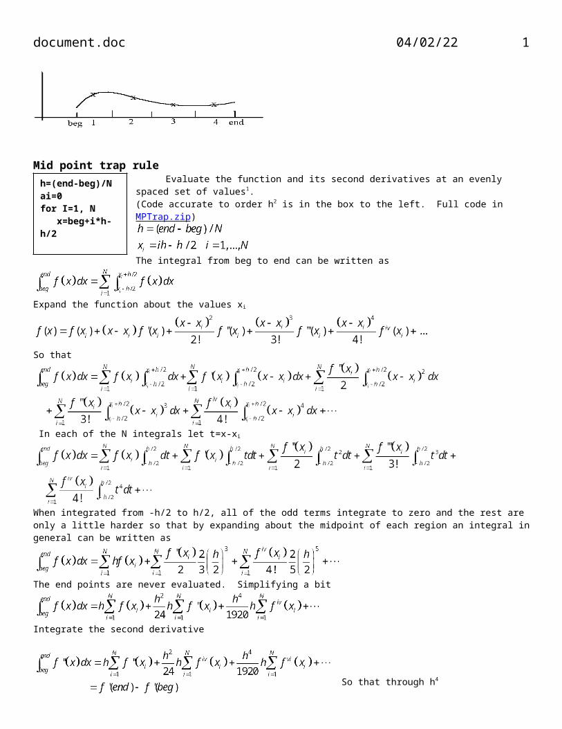
h=(end-beg)/N ai=0 for I=1, N x=beg+i*h- h/2 document.doc 04/02/22 Mid point trap rule Evaluate the function and its second derivatives at an evenly spaced set of values 1 . (Code accurate to order h 2 is in the box to the left. Full code in MPTrap.zip ) The integral from beg to end can be written as Expand the function about the values x i So that In each of the N integrals let t=x-x i When integrated from -h/2 to h/2, all of the odd terms integrate to zero and the rest are only a little harder so that by expanding about the midpoint of each region an integral in general can be written as The end points are never evaluated. Simplifying a bit Integrate the second derivative So that through h 4 1

Welcome message from author
This document is posted to help you gain knowledge. Please leave a comment to let me know what you think about it! Share it to your friends and learn new things together.
Transcript
h=(end-beg)/Nai=0for I=1, N x=beg+i*h-h/2 ai=ai+fun(x)enddoai=ai ´ h
document.doc 05/16/23
Mid point trap rule Evaluate the function and its second derivatives at an evenly spaced set of values1.
(Code accurate to order h2 is in the box to the left. Full code in MPTrap.zip)
The integral from beg to end can be written as
Expand the function about the values xi
So that
In each of the N integrals let t=x-xi
When integrated from -h/2 to h/2, all of the odd terms integrate to zero and the rest are only a little harder so that by expanding about the midpoint of each region an integral in general can be written as
The end points are never evaluated. Simplifying a bit
Integrate the second derivative
So that through h4
1
document.doc 05/16/23
So that
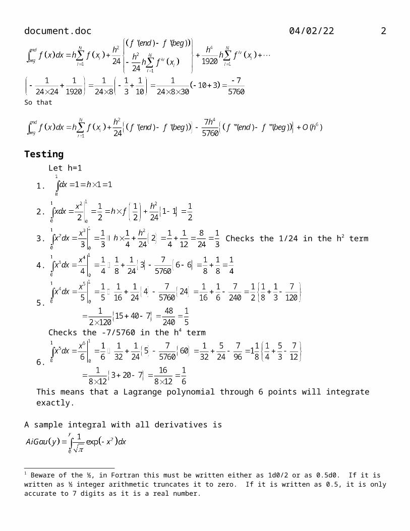
TestingLet h=1
1.
2.
3. Checks the 1/24 in the h2 term
4.
5.
Checks the -7/5760 in the h4 term
6.
This means that a Lagrange polynomial through 6 points will integrate exactly.
A sample integral with all derivatives is
2
document.doc 05/16/23
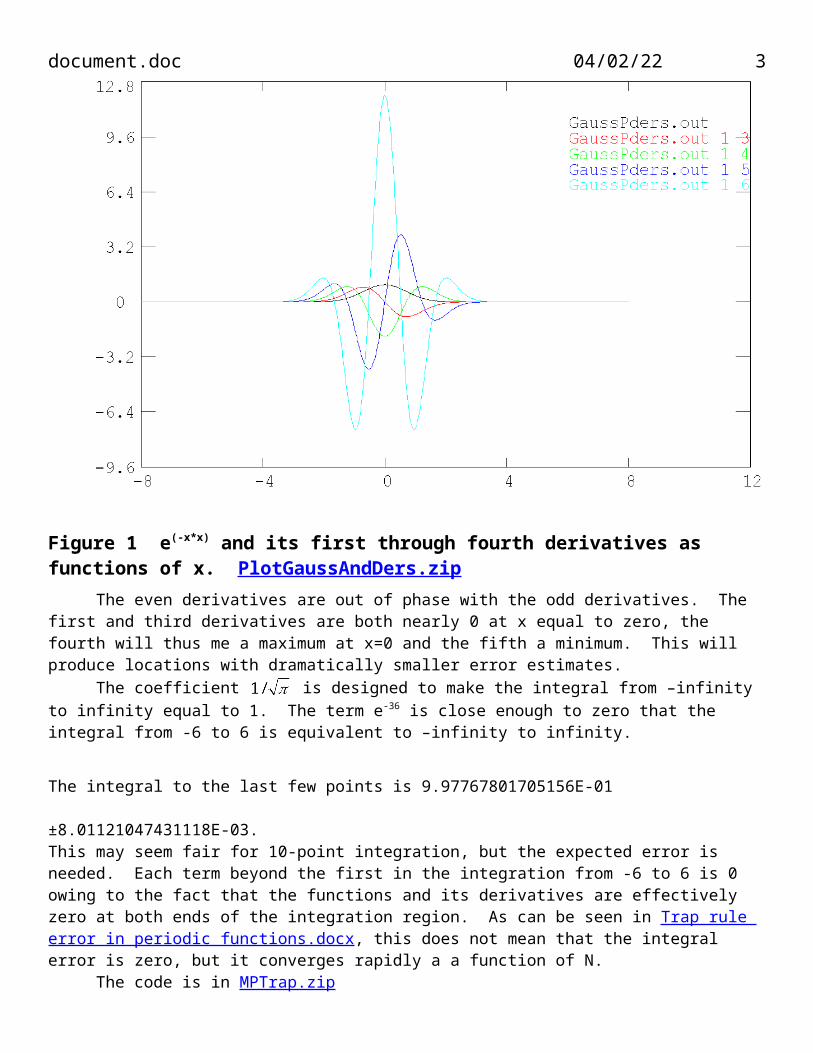
Figure 1 e(-x*x) and its first through fourth derivatives as functions of x. PlotGaussAndDers.zip The even derivatives are out of phase with the odd derivatives. The first and third derivatives are both nearly 0 at x equal to zero, the fourth will thus me a maximum at x=0 and the fifth a minimum. This will produce locations with dramatically smaller error estimates.
The coefficient is designed to make the integral from –infinity to infinity equal to 1. The term e-
36 is close enough to zero that the integral from -6 to 6 is equivalent to –infinity to infinity.
The integral to the last few points is 9.97767801705156E-01 ±8.01121047431118E-03.This may seem fair for 10-point integration, but the expected error is needed. Each term beyond the first in the integration from -6 to 6 is 0 owing to the fact that the functions and its derivatives are effectively zero at both ends of the integration region. As can be seen in Trap rule error in periodic functions.docx, this does not mean that the integral error is zero, but it converges rapidly a a function of N.
The code is in MPTrap.zip
3
document.doc 05/16/23
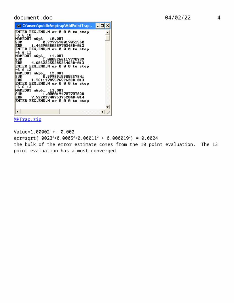
MPTrap.zip
Value=1.00002 +- 0.002err≅sqrt(.00232+0.00052+0.000112 + 0.0000192) = 0.0024the bulk of the error estimate comes from the 10 point evaluation. The 13 point evaluation has almost converged.
1 Beware of the ½, in Fortran this must be written either as 1d0/2 or as 0.5d0. If it is written as ½ integer arithmetic truncates it to zero. If it is written as 0.5, it is only accurate to 7 digits as it is a real number.
4
document.doc 05/16/23
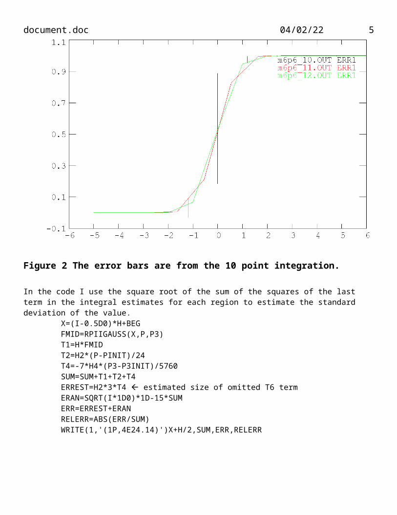
Figure 2 The error bars are from the 10 point integration.
In the code I use the square root of the sum of the squares of the last term in the integral estimates for each region to estimate the standard deviation of the value. X=(I-0.5D0)*H+BEG FMID=RPIIGAUSS(X,P,P3) T1=H*FMID T2=H2*(P-PINIT)/24 T4=-7*H4*(P3-P3INIT)/5760 SUM=SUM+T1+T2+T4 ERREST=H2*3*T4 estimated size of omitted T6 term ERAN=SQRT(I*1D0)*1D-15*SUM ERR=ERREST+ERAN RELERR=ABS(ERR/SUM) WRITE(1,'(1P,4E24.14)')X+H/2,SUM,ERR,RELERR
5
document.doc 05/16/23
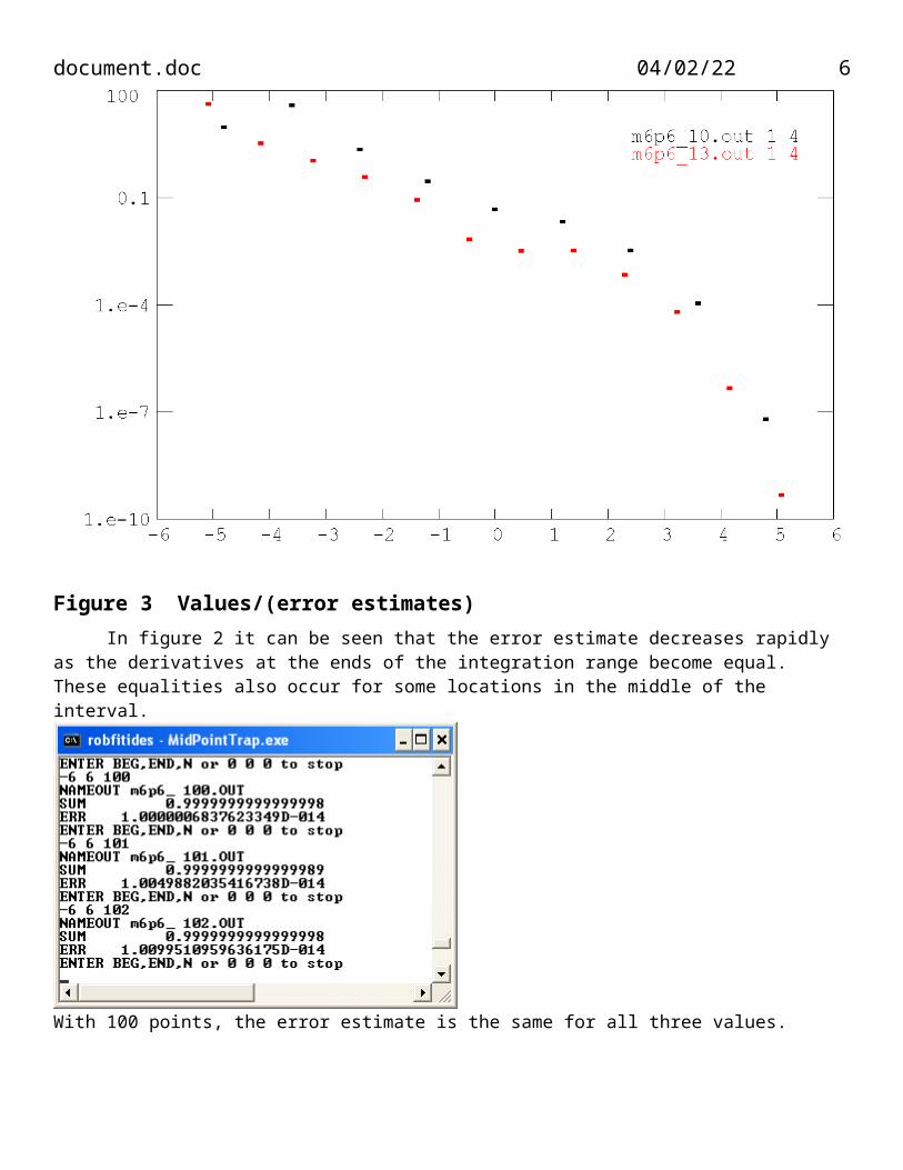
Figure 3 Values/(error estimates)In figure 2 it can be seen that the error estimate decreases rapidly as the derivatives at the ends of the
integration range become equal. These equalities also occur for some locations in the middle of the interval.
With 100 points, the error estimate is the same for all three values.
6
document.doc 05/16/23
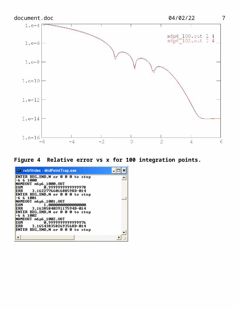
Figure 4 Relative error vs x for 100 integration points.
7
document.doc 05/16/23
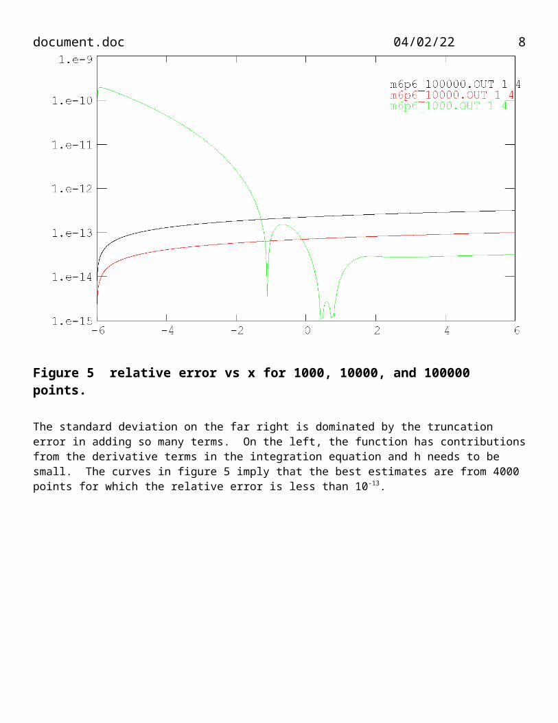
Figure 5 relative error vs x for 1000, 10000, and 100000 points.
The standard deviation on the far right is dominated by the truncation error in adding so many terms. On the left, the function has contributions from the derivative terms in the integration equation and h needs to be small. The curves in figure 5 imply that the best estimates are from 4000 points for which the relative error is less than 10-13.
8
Related Documents