Transport in the Hudson Estuary: A Modeling Study of ...water.columbia.edu/files/2011/11/Lall2004Transport.pdf · Transport in the Hudson Estuary: A Modeling Study of Estuarine Circulation

Estuaries Vol. 27, No. 3, p. 527-538 June 2004

Transport in the Hudson Estuary: A Modeling Study of Estuarine

Circulation and Tidal Trapping

FERDI L. HELLWEGER1'2,*, ALAN F. BLUMBERG2'3, PETER SCHLOSSER1'4'5, DAVID T. HO4,5, THEODORE CAPLOW1, UPMANU LALL1, and HONGHAI LI2

1 Department of Earth and Environmental Engineering, Columbia University, 500 West 120th Street, New York, New York 10027

2 HydroQual, Inc., 1200 MacArthur Boulevard, Mahwah, New Jersey 07430 3 Stevens Institute of Technology, Castle Point on Hudson, Hoboken, New Jersey 07030 4 Lamont-Doherty Earth Observatory, Columbia University, 61 Route 9W, Palisades, New York

10964 5 Department of Earth and Environmental Sciences, Columbia University, New York, New York

10027

ABSTRACT: The effects of estuarine circulation and tidal trapping on transport in the Hudson estuary were investi- gated by a large-scale, high-resolution numerical model simulation of a tracer release. The modeled and measured longitudinal profiles of surface tracer concentrations (plumes) differ from the ideal Gaussian shape in two ways: on a large scale the plume is asymmetric with the downstream end stretching out farther, and small-scale (1-2 km) peaks are present at the upstream and downstream ends of the plume. A number of diagnostic model simulations (e.g., remove freshwater flow) were performed to understand the processes responsible for these features. These simulations show that the large-scale asymmetry is related to salinity. The salt causes an estuarine circulation that decreases vertical mixing (vertical density gradient), increases longitudinal dispersion (increased vertical and lateral gradients in longitudinal velocities), and increases net downstream velocities in the surface layer. Since salinity intrusion is confined to the downstream end of the tracer plume, only that part of the plume is effected by those processes, which leads to the large- scale asymmetry. The small-scale peaks are due to tidal trapping. Small embayments along the estuary trap water and tracer as the plume passes by in the main channel. When the plume in the main channel has passed, the tracer is released back to the main channel, caiising a secondary peak in the longitudinal profile.

Introduction

Understanding the transport characteristics of the Hudson River estuary is important for predict- ing the fate of contaminants discharged there. Es- tuarine transport can be studied by observation as well as analytical and numerical modeling. Where- as either of these approaches can be used alone, the combination of data and model is the most effective approach because observational and modeling strategies complement each other. Data can be used to calibrate and validate a model and models help understand the physics governing natural systems and extrapolate data to areas and times with little or no coverage.

Continued improvements in analytical tech- niques provide us with the capability to observe tracers released into a water body at much higher temporal and spatial resolution. This allows for a much more sophisticated model calibration. At the same time computational power increases and with

* Corresponding author; tele: 201/529-5151; fax: 201/529- 5728; e-mail: [email protected]

it the spatial resolution of numerical estuarine models. The result is greater realism, but also increased complexity, which makes models more difficult to understand. High-resolution models of complex natural systems, such as the Hudson estuary, frequently produce features that are intui- tively difficult to explain; diagnosing such features is important for understanding the model and the real system. Advanced model diagnostic tools that allow for the visualization of computed parameters (e.g., animations of surface currents) are crucial for understanding the behavior of models. They are, in essence, tools for observing the model system, as data collection is a tool for observing the natural system. Another diagnostic strategy, which is typically not possible with the natural system, is to modify the model forcing functions and coeffi- cients systematically and observe the effect on the simulated variables. Salt can be removed to understand its effect on the transport of constituents dissolved in the water. This technique is commonly used to understand the sensitivity of model results to the values of various input parameters (e.g., un-

? 2004 Estuarine Research Federation 527

watercenter

Stamp

528 F. L. Hellweger et al.

certainty analysis). It can also be used to identify and understand the mechanisms controlling the behavior of models. We used diagnostic simulations to understand the behavior of a model and the physical processes operating in the Hudson estuary.

In this contribution a numerical simulation of a tracer release into the Hudson estuary is presented. The study combines high-resolution tracer sampling (over 2,000 samples, 400 m resolution) and modeling (over 10,000 mass balance segments; 600 m horizontal, 1 m vertical resolution in the study area). An existing model presented by Blumberg et al. (2004) is used to simulate the fate and transport of SF6 released in a field study presented by Ho et al. (2002).

STUDY AREA

The Hudson River starts at Lake Tear of the Clouds in the Adirondack Mountains and ends in New York City. The 248 km stretch below Troy, New York, is commonly referred to as the Hudson estuary. Freshwater inflow into the estuary occurs predominantly from the Upper Hudson River at Troy at an average rate of 392 m3 s-1. Smaller trib- utaries, like Wappinger Creek (7 m3 s-1), also discharge downstream of that point. The flow of the Upper Hudson River is seasonal, highest during winter and spring and lowest in the summer. As a result the salinity intrusion is also seasonal. In the spring the salt front is located near Yonkers, New York, and in the summer it is located by Newburgh, New York. The hydrodynamics of the Hudson estuary have been studied by Steward (1958), Prit- chard et al. (1962), Abood (1974), Hunkins (1981), and Geyer et al. (2000).

DATA

In the summer of 2001 a large-scale SF6 tracer release experiment was conducted in the Hudson estuary (Ho et al. 2002). On July 25, 2001, roughly 4.3 mol of SF6 gas were injected at 5 m depth near Newburgh (Fig. 1; kilometer point (KMP) 98; dis- tances are referenced to the Battery at the southern tip of Manhattan) from a boat while twice tra- versing the estuary laterally over a period of 28 min. The release time (12:14-12:42) approximately corresponds to slack before flood (SBF) at New- burgh. Based on subsequent concentration measurements, Ho et al. (2002) estimated that of the 4.3 mol injected approximately 1.1 mol dissolved in the water, and the remainder escaped to the atmosphere in the form of bubbles. SF6 is an inert gas and consequently is lost from the water column only by gas exchange across the air-water interface. On the basis of a mass balance, Ho et al. (2002) estimated an average gas transfer velocity for SF6

7A4?n' W 73*R5 W

- '

-115 q z

-110

WAPPINGER CREEK

100

f RELEASE

KMP 88 X .

-- - 7 ? '

^^^ --95 o_9

' ' IONA ISLAND .-90

. ~85

WORLD'S END

-80

z

-' --75 '

IONA ISLAND z ..KMP 73

7400, W 73?55' W

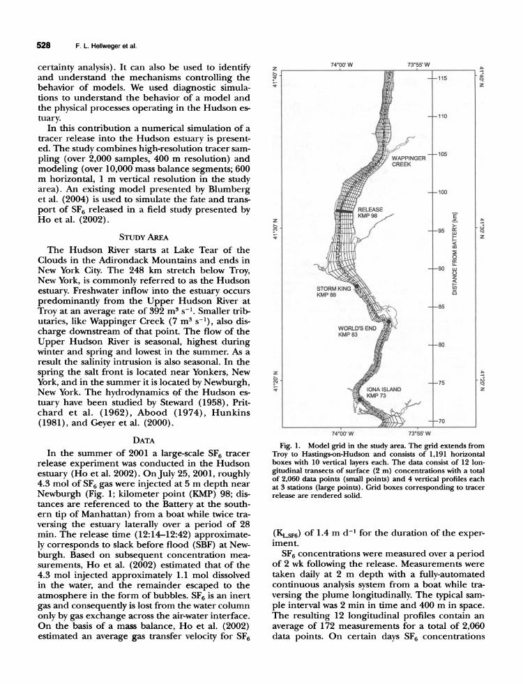
Fig. 1. Model grid in the study area. The grid extends from Troy to Hastings-on-Hudson and consists of 1,191 horizontal boxes with 10 vertical layers each. The data consist of 12 longitudinal transects of surface (2 m) concentrations with a total of 2,060 data points (small points) and 4 vertical profiles each at 3 stations (large points). Grid boxes corresponding to tracer release are rendered solid.

(KL,sF6) of 1.4 m d-1 for the duration of the experiment.

SF6 concentrations were measured over a period of 2 wk following the release. Measurements were taken daily at 2 m depth with a fully-automated continuous analysis system from a boat while tra- versing the plume longitudinally. The typical sample interval was 2 min in time and 400 m in space. The resulting 12 longitudinal profiles contain an average of 172 measurements for a total of 2,060 data points. On certain days SF6 concentrations

Transport in the Hudson Estuary 529

were measured at several depths at various locations (Fig. 1).

MODEL

The model, described in detail by Blumberg et al. (2004), is based on the three-dimensional, time- variable, estuarine and coastal circulation modeling framework. It is an estuarine and coastal ver- sion of the Princeton Ocean Model (Blumberg and Mellor 1987), incorporating the Mellor-Ya- mada 2.5 level turbulent closure model that pro- vides a realistic parameterization of vertical mixing processes. A curvilinear horizontal segmentation allows for smooth and accurate representation of shoreline geometry, and a sigma-level vertical coordinate system permits better representation of bottom topography. The model solves a coupled system of differential, prognostic equations de- scribing the conservation of mass, momentum, salinity, temperature, turbulent energy, and a length scale characterizing the size of the turbulent ed- dies. A recent application of the model to St. An- drew Bay, Florida, is presented by Blumberg and Kim (2000). A detailed description of the model's governing equations can be found in Blumberg et al. (1999) and HydroQual (2001).

The model covers 209 km of the Hudson estuary from Hastings-on-Hudson, New York, to Troy. It consists of 1,191 horizontal grid boxes, each with 10 vertical layers, for a total of 11,910 mass balance segments. The model is forced with discharge from five rivers (Upper Hudson River, Esopus Creek, Rondout Creek, Wappinger Creek, and Croton River), atmospheric heat flux, wind stress (based on data at Albany and New York City), and water surface elevation, salinity, and temperature at the downstream boundary (Hastings-on-Hudson). Withdrawal and discharge rates and temperature rise of five power plants (Danskammer Point, Ro- seton, Indian Point, Lovett, and Bowline Point) are specified as input. The model was originally set up to simulate the periods March 11, 1998-April 9, 1998 (high flow), and August 1-30, 1997 (low flow), and validated extensively against field data including water surface elevation, salinity, and temperature at various locations, shipboard acoustic Doppler current profile (ADCP) velocity, salinity, and temperature measurements, and fixed-site ADCP velocity, salinity, and temperature measurements -as described by Blumberg et al. (2004).

TRACER SIMULATION

Model Set-up For the tracer simulation the model forcing

functions were updated for the period July 10, 2001-August 9, 2001, allowing for 15 d of spin-up before the tracer release on July 25, 2001. The

model boundary conditions (freshwater flow rate, wind speed, wind direction, and downstream boundary water surface elevation) were assigned based on data. The mean flow rate for the model period of the Hudson River at Troy was 140 m3 s-1. Salinity and temperature for the start of the simulation (initial conditions) were not available. They were specified based on ship surveys before and after the start date (June 15, 2001, July 28, 2001) and surface measurements at the U.S. Geo- logical Survey gage at Hastings-on-Hudson. Power plant intake and outfall data for the new period were not available and were kept the same as for the original low flow period.

SF6 was added to the model at a constant loading rate (mol s-1) over a period of 28 min at KMP 98, distributed equally over the 10 lateral grid boxes (Fig. 1) and the top 5 vertical layers (corresponding to approximately 5 m). Ho et al. (2002) injected 4.3 mol, of which they estimated 1.1 mol dissolved. Their estimate was based on subsequent SF6 inventory estimates, and in a similar manner the total mass added to the model was adjusted here to match the SF6 concentration profiles, resulting in an addition of 1.6 mol to the model. To simulate SF6 gas exchange a constant gas transfer velocity (Kl,SF6, m d-1) was specified. This velocity was divided by the depth of the top layer to yield a first-order decay rate, which was applied to the top layer. This assumes the atmospheric gas concentration is negligible, which is a safe assumption for this study. The approach is relatively crude, in that it neglects the effect of varying wind speed on the gas transfer velocity (Wanninkhof 1992) and assumes the tracer is vertically and uniformly mixed over the top layer. A constant gas transfer velocity of KL,SF6

= 1.4 m d-1 as estimated by Ho et al. (2002) was used.

The horizontal dispersion used by Blumberg et al. (2004) was based on calibration to relatively small horizontal gradients in salinity. Initial simulations of the SF6 tracer release using the same coefficient of dispersion (Cs = 0.10; Cs is the constant in the dispersion formulation by Smagorinsky [1963]), as used by Blumberg et al. (2004), result- ed in an underestimation of the dispersion of SF6. The Cs coefficient was recalibrated to match observed tracer concentrations resulting in a value of 0.01. This is within the range of other applications (Ezer and Mellor 2000; HydroQual 2001), but at first glance, it is surprising that such a large change is required. To illustrate the effect of the Cs coefficient (and to validate the model performance), a model-data comparison using both Cs values is presented for salinity and SF6 in Figs. 2 and 3, respectively. A more extensive model-data comparison for SF6 concentrations will be presented in the


lu

CS = 0.10 o Data- Surface .- Model - Surface

^Y^> ~~~~: * Data- Bottom

^^^< ,~~~~ - Model - Bottom 5 .

0 . I

r-

'a

0

I- z

o 0

Lf c(

60 80 100

DISTANCE FROM BATTERY [km]

120

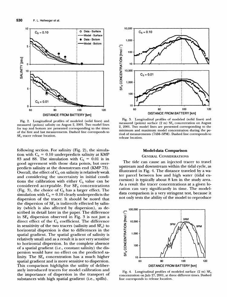
Fig. 2. Longitudinal profiles of modeled (solid lines) and measured (points) salinity on August 2, 2001. Two model lines for top and bottom are presented corresponding to the times of the first and last measurements. Dashed line corresponds to SF6 tracer release location.

following section. For salinity (Fig. 2), the simulation with Cs = 0.10 underpredicts salinity at KMP 83 and 88. The simulation with Cs = 0.01 is in good agreement with those data points, but over- predicts salinity at the downstream end (KMP 73). Overall, the effect of Cs on salinity is relatively weak and considering the uncertainty in initial conditions the calibration with either Cs value can be considered acceptable. For SF6 concentrations (Fig. 3), the choice of Cs has a larger effect. The simulation with Cs = 0.10 clearly underpredicts the dispersion of the tracer. It should be noted that the dispersion of SF6 is indirectly effected by salinity (which is also affected by dispersion), as described in detail later in the paper. The difference in SF6 dispersion observed in Fig. 3 is not just a direct effect of the Cs coefficient. The difference in sensitivity of the two tracers (salinity and SF6) to horizontal dispersion is due to differences in the spatial gradient. The spatial gradient of salinity is relatively small and as a result it is not very sensitive to horizontal dispersion. In the complete absence of a spatial gradient (i.e., constant salinity) the dispersion would have no effect on the predicted salinity. The SF6 concentration has a much higher spatial gradient and is more sensitive to dispersion. This comparison highlights the utility of deliber- ately introduced tracers for model calibration and the importance of dispersion in the transport of substances with high spatial gradient (i.e., spills).

120 . I - I .

60 80 100


Fig. 3. Longitudinal profiles of modeled (solid lines) and measured (points) surface (2 m) SF6 concentration on August 2, 2001. Two model lines are presented corresponding to the minimum and maximum model concentration during the period of measurements (7AM-5PM). Dashed line corresponds to release location.

Model-data Comparison GENERAL CONSIDERATIONS

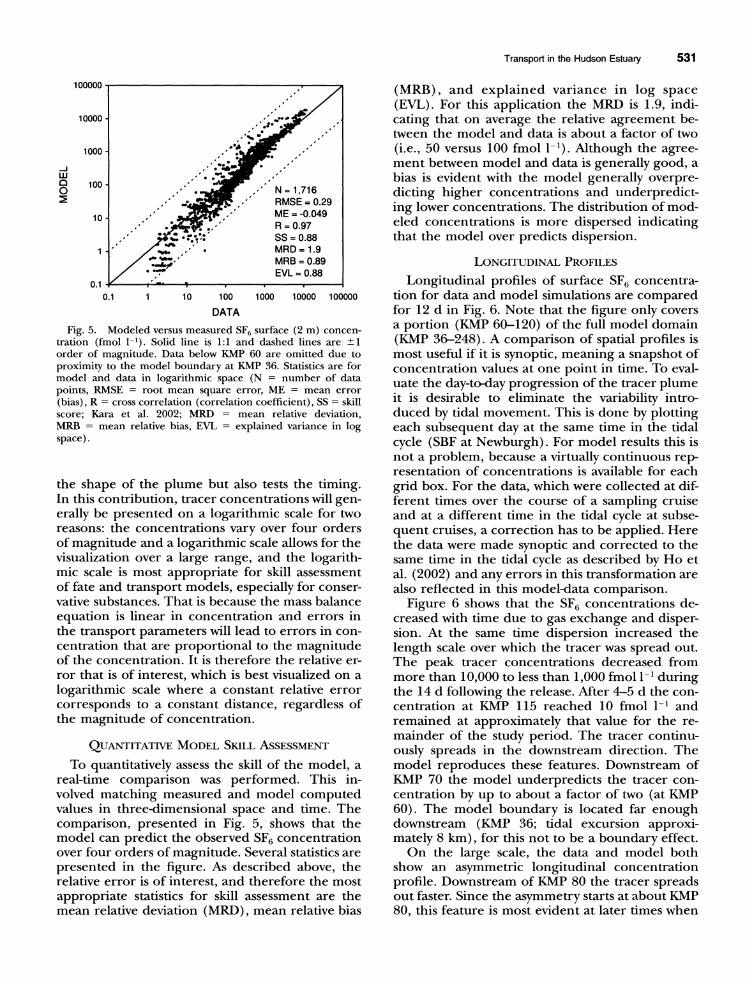
The tide can cause an injected tracer to travel upstream and downstream within the tidal cycle, as illustrated in Fig. 4. The distance traveled by a water parcel between low and high water (tidal excursion) is typically about 8 km in the study area. As a result the tracer concentrations at a given location can vary significantly in time. The model- data comparison is a very stringent test, because it not only tests the ability of the model to reproduce

-

z 0

I-

LU 0 z

0 0 o

(/

60 80 100


120

Fig. 4. Longitudinal profiles of modeled surface (2 m) SF6 concentration on July 27, 2001, at three different times. Dashed line corresponds to release location.

10,000

1,000

100

10

3

0Q

r Z 10

5


100000

10000

1000

-J w 0 0 100

10 - . -

, ? :' '

-. . ...SS= 0.88 1 -'' /~ ,,, * MRD= 1.9

"/ "=,' MRB= 0.89 EVL= 0.88

0.1 i' , 0.1 1 10 100 1000 10000 100000

DATA

Fig. 5. Modeled versus measured SF6 surface (2 m) concentration (fmol 1-1). Solid line is 1:1 and dashed lines are ?1 order of magnitude. Data below KMP 60 are omitted due to proximity to the model boundary at KMP 36. Statistics are for model and data in logarithmic space (N = number of data points, RMSE = root mean square error, ME = mean error (bias), R = cross correlation (correlation coefficient), SS = skill score; Kara et al. 2002; MRD = mean relative deviation, MRB = mean relative bias, EVL = explained variance in log space).

the shape of the plume but also tests the timing. In this contribution, tracer concentrations will generally be presented on a logarithmic scale for two reasons: the concentrations vary over four orders of magnitude and a logarithmic scale allows for the visualization over a large range, and the logarithmic scale is most appropriate for skill assessment of fate and transport models, especially for conservative substances. That is because the mass balance equation is linear in concentration and errors in the transport parameters will lead to errors in concentration that are proportional to the magnitude of the concentration. It is therefore the relative error that is of interest, which is best visualized on a logarithmic scale where a constant relative error corresponds to a constant distance, regardless of the magnitude of concentration.

QUANTITATIVE MODEL SKILL ASSESSMENT

To quantitatively assess the skill of the model, a real-time comparison was performed. This in- volved matching measured and model computed values in three-dimensional space and time. The comparison, presented in Fig. 5, shows that the model can predict the observed SF6 concentration over four orders of magnitude. Several statistics are presented in the figure. As described above, the relative error is of interest, and therefore the most appropriate statistics for skill assessment are the mean relative deviation (MRD), mean relative bias

(MRB), and explained variance in log space (EVL). For this application the MRD is 1.9, indicating that on average the relative agreement between the model and data is about a factor of two (i.e., 50 versus 100 fmol 1-1). Although the agreement between model and data is generally good, a bias is evident with the model generally overpre- dicting higher concentrations and underpredict- ing lower concentrations. The distribution of modeled concentrations is more dispersed indicating that the model over predicts dispersion.

LONGITUDINAL PROFILES

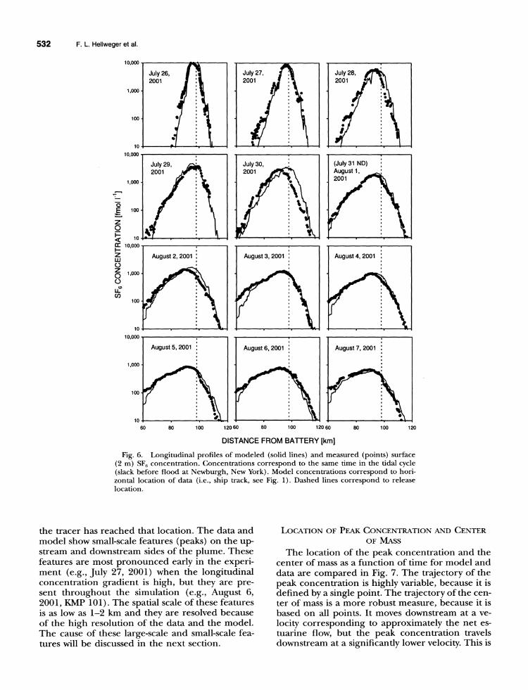
Longitudinal profiles of surface SF6 concentration for data and model simulations are compared for 12 d in Fig. 6. Note that the figure only covers a portion (KMP 60-120) of the full model domain (KMP 36-248). A comparison of spatial profiles is most useful if it is synoptic, meaning a snapshot of concentration values at one point in time. To eval- uate the day-to-day progression of the tracer plume it is desirable to eliminate the variability introduced by tidal movement. This is done by plotting each subsequent day at the same time in the tidal cycle (SBF at Newburgh). For model results this is not a problem, because a virtually continuous representation of concentrations is available for each grid box. For the data, which were collected at different times over the course of a sampling cruise and at a different time in the tidal cycle at subsequent cruises, a correction has to be applied. Here the data were made synoptic and corrected to the same time in the tidal cycle as described by Ho et al. (2002) and any errors in this transformation are also reflected in this model-data comparison.

Figure 6 shows that the SF6 concentrations decreased with time due to gas exchange and dispersion. At the same time dispersion increased the length scale over which the tracer was spread out. The peak tracer concentrations decreased from more than 10,000 to less than 1,000 fmol 1-1 during the 14 d following the release. After 4-5 d the concentration at KMP 115 reached 10 fmol 1-1 and remained at approximately that value for the remainder of the study period. The tracer continu- ously spreads in the downstream direction. The model reproduces these features. Downstream of KMP 70 the model underpredicts the tracer concentration by up to about a factor of two (at KMP 60). The model boundary is located far enough downstream (KMP 36; tidal excursion approximately 8 km), for this not to be a boundary effect.

On the large scale, the data and model both show an asymmetric longitudinal concentration profile. Downstream of KMP 80 the tracer spreads out faster. Since the asymmetry starts at about KMP 80, this feature is most evident at later times when


10,000

July 26, 2001

1,000 -

100 -

10 p

10,000

1,000 -

-

o E 100-

z 0

10

I-

CO

-100

10

10,000

1,000-

100

10 10

. ''\ August 2, 2001 '

60 80 100

August 3, 2001

August 6, 2001

120 6( D 80 100 1

August 4, 2001

20 60 80 100 120


Fig. 6. Longitudinal profiles of modeled (solid lines) and measured (points) surface (2 m) SF6 concentration. Concentrations correspond to the same time in the tidal cycle (slack before flood at Newburgh, New York). Model concentrations correspond to horizontal location of data (i.e., ship track, see Fig. 1). Dashed lines correspond to release location.

the tracer has reached that location. The data and model show small-scale features (peaks) on the upstream and downstream sides of the plume. These features are most pronounced early in the experiment (e.g., July 27, 2001) when the longitudinal concentration gradient is high, but they are present throughout the simulation (e.g., August 6, 2001, KMP 101). The spatial scale of these features is as low as 1-2 km and they are resolved because of the high resolution of the data and the model. The cause of these large-scale and small-scale features will be discussed in the next section.

LOCATION OF PEAK CONCENTRATION AND CENTER OF MASS

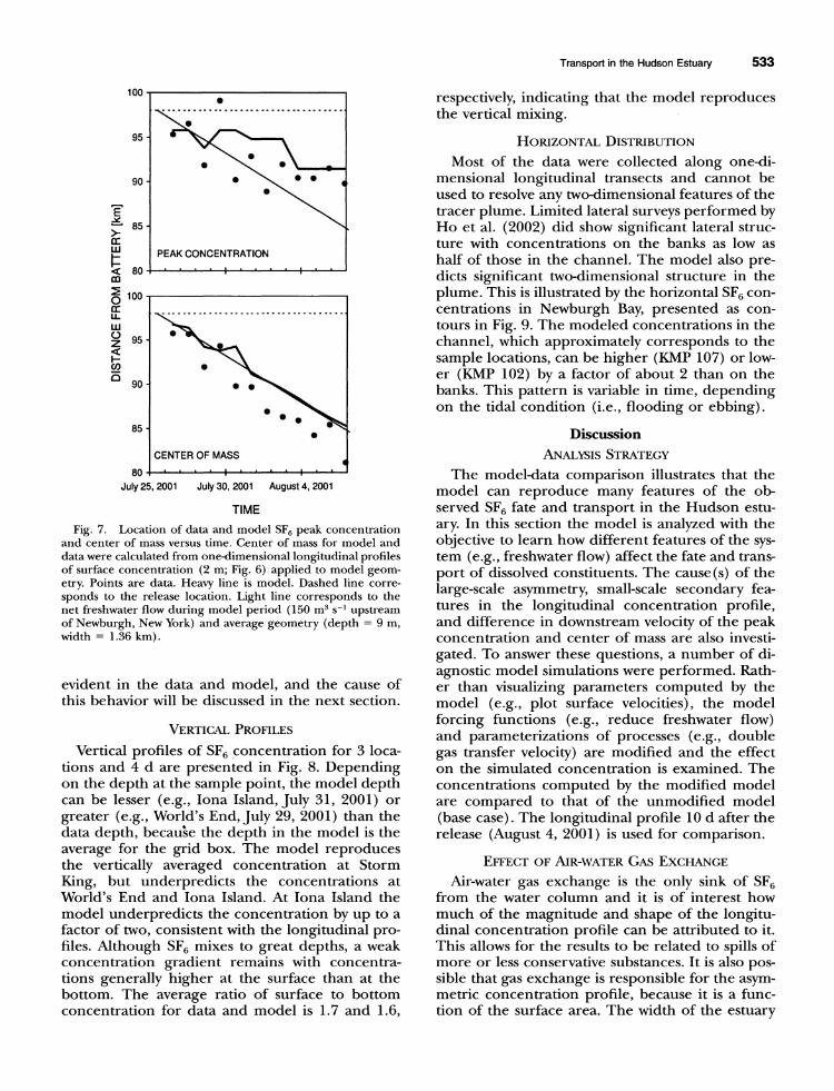
The location of the peak concentration and the center of mass as a function of time for model and data are compared in Fig. 7. The trajectory of the peak concentration is highly variable, because it is defined by a single point. The trajectory of the center of mass is a more robust measure, because it is based on all points. It moves downstream at a velocity corresponding to approximately the net estuarine flow, but the peak concentration travels downstream at a significantly lower velocity. This is

4


E 85-

t?! PEAK CONCENTRATION

<80 ... . I .

O 100

C:. ..................................

90-

85 -

CENTER OF MASS

80 . . . . . I July 25, 2001 July 30, 2001 August 4, 2001

TIME

Fig. 7. Location of data and model SF6 peak concentration and center of mass versus time. Center of mass for model and data were calculated from one-dimensional longitudinal profiles of surface concentration (2 m; Fig. 6) applied to model geometry. Points are data. Heavy line is model. Dashed line corresponds to the release location. Light line corresponds to the net freshwater flow during model period (150 m3 s-1 upstream of Newburgh, New York) and average geometry (depth = 9 m, width = 1.36 km).

evident in the data and model, and the cause of this behavior will be discussed in the next section.

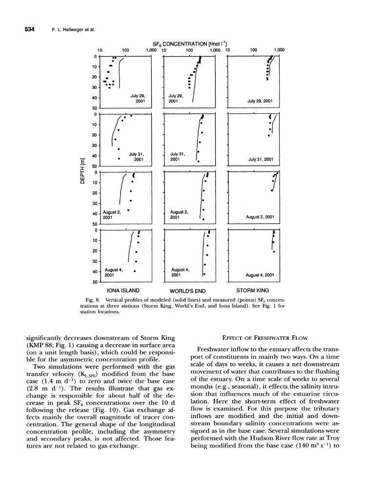
VERTICAL PROFILES

Vertical profiles of SF6 concentration for 3 locations and 4 d are presented in Fig. 8. Depending on the depth at the sample point, the model depth can be lesser (e.g., Iona Island, July 31, 2001) or greater (e.g., World's End, July 29, 2001) than the data depth, because the depth in the model is the average for the grid box. The model reproduces the vertically averaged concentration at Storm King, but underpredicts the concentrations at World's End and Iona Island. At Iona Island the model underpredicts the concentration by up to a factor of two, consistent with the longitudinal profiles. Although SF6 mixes to great depths, a weak concentration gradient remains with concentrations generally higher at the surface than at the bottom. The average ratio of surface to bottom concentration for data and model is 1.7 and 1.6,

respectively, indicating that the model reproduces the vertical mixing.

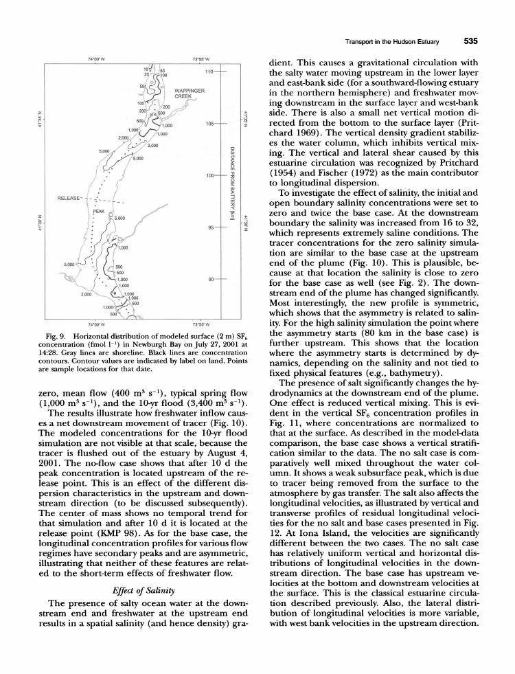
HORIZONTAL DISTRIBUTION

Most of the data were collected along one-dimensional longitudinal transects and cannot be used to resolve any two-dimensional features of the tracer plume. Limited lateral surveys performed by Ho et al. (2002) did show significant lateral structure with concentrations on the banks as low as half of those in the channel. The model also predicts significant two-dimensional structure in the plume. This is illustrated by the horizontal SF6 concentrations in Newburgh Bay, presented as contours in Fig. 9. The modeled concentrations in the channel, which approximately corresponds to the sample locations, can be higher (KMP 107) or lower (KMP 102) by a factor of about 2 than on the banks. This pattern is variable in time, depending on the tidal condition (i.e., flooding or ebbing).

Discussion ANALYSIS STRATEGY

The model-data comparison illustrates that the model can reproduce many features of the observed SF6 fate and transport in the Hudson estuary. In this section the model is analyzed with the objective to learn how different features of the system (e.g., freshwater flow) affect the fate and transport of dissolved constituents. The cause (s) of the large-scale asymmetry, small-scale secondary features in the longitudinal concentration profile, and difference in downstream velocity of the peak concentration and center of mass are also investi- gated. To answer these questions, a number of diagnostic model simulations were performed. Rath- er than visualizing parameters computed by the model (e.g., plot surface velocities), the model forcing functions (e.g., reduce freshwater flow) and parameterizations of processes (e.g., double gas transfer velocity) are modified and the effect on the simulated concentration is examined. The concentrations computed by the modified model are compared to that of the unmodified model (base case). The longitudinal profile 10 d after the release (August 4, 2001) is used for comparison.

EFFECT OF AIR-WATER GAS EXCHANGE

Air-water gas exchange is the only sink of SF6 from the water column and it is of interest how much of the magnitude and shape of the longitudinal concentration profile can be attributed to it. This allows for the results to be related to spills of more or less conservative substances. It is also possible that gas exchange is responsible for the asymmetric concentration profile, because it is a function of the surface area. The width of the estuary


10 100 1,C 0

. / 10- e

20- .

30'-

40 - July 29, 2001

50

0 /

10 -

20 -

30 -

40 - July 31, * 2001

50 0

10 -

20-

30-

40-

50 0

10 -

20-

30-

40-

50

/ {

August 2, 2001

SF6 CONCENTRATION [fmol 1-'1] )00 10 100 1,000 10 100 1,000

f I

July 29, -

2001 / July 29, 2001

August 2, 2001

*

August 4, 2001

August 4, 2001 *

July 31, 2001

JI,

August 2, 2001

August 4, 2001

IONA ISLAND WORLD'S END STORM KING

Fig. 8. Vertical profiles of modeled (solid lines) and measured (points) SF6 concentrations at three stations (Storm King, World's End, and Iona Island). See Fig. 1 for station locations.

significantly decreases downstream of Storm King (KMP 88; Fig. 1) causing a decrease in surface area (on a unit length basis), which could be responsible for the asymmetric concentration profile.

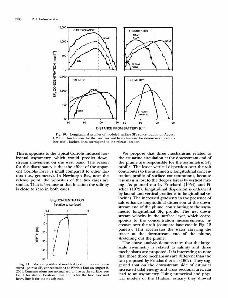
Two simulations were performed with the gas transfer velocity (KL,SF6) modified from the base case (1.4 m d-1) to zero and twice the base case (2.8 m d-l1). The results illustrate that gas exchange is responsible for about half of the decrease in peak SF6 concentrations over the 10 d following the release (Fig. 10). Gas exchange affects mainly the overall magnitude of tracer concentration. The general shape of the longitudinal concentration profile, including the asymmetry and secondary peaks, is not affected. Those features are not related to gas exchange.

EFFECT OF FRESHWATER FLOW

Freshwater inflow to the estuary affects the transport of constituents in mainly two ways. On a time scale of days to weeks, it causes a net downstream movement of water that contributes to the flushing of the estuary. On a time scale of weeks to several months (e.g., seasonal), it effects the salinity intrusion that influences much of the estuarine circulation. Here the short-term effect of freshwater flow is examined. For this purpose the tributary inflows are modified and the initial and downstream boundary salinity concentrations were assigned as in the base case. Several simulations were performed with the Hudson River flow rate at Troy being modified from the base case (140 m3 s-1) to

E I

0 IJJ cQ

*

*


7400' W 7355' W

10J.J 50 110--- 20 -f 100

5C o WAPPINGER CREEK

100 / / 200 200 500

500/~'1,000 105 1,000 XA- 1.000 k,1,000

2,0001

. 2,000

5,000 > z

O .*~~ <~~100- ; 0

RELEASE- - -

-<

PEAK

5,000 3

95

5 ( ' 1,000

*5 000" * ^500

,f' ~--1,000 90- ,5 000 1 000

2,000 SO-1,000 1 000 25 500

1,000 500

500 0 t,ooh

74'00' W 73'55' W

Fig. 9. Horizontal distribution of modeled surface (2 m) SF6 concentration (fmol 1-1) in Newburgh Bay on July 27, 2001 at 14:28. Gray lines are shoreline. Black lines are concentration contours. Contour values are indicated by label on land. Points are sample locations for that date.

zero, mean flow (400 m3 s-1), typical spring flow (1,000 m3 s-1), and the 10-yr flood (3,400 m3 s-1).

The results illustrate how freshwater inflow causes a net downstream movement of tracer (Fig. 10). The modeled concentrations for the 10-yr flood simulation are not visible at that scale, because the tracer is flushed out of the estuary by August 4, 2001. The no-flow case shows that after 10 d the peak concentration is located upstream of the release point. This is an effect of the different dispersion characteristics in the upstream and downstream direction (to be discussed subsequently). The center of mass shows no temporal trend for that simulation and after 10 d it is located at the release point (KMP 98). As for the base case, the longitudinal concentration profiles for various flow regimes have secondary peaks and are asymmetric, illustrating that neither of these features are related to the short-term effects of freshwater flow.

Effect of Salinity The presence of salty ocean water at the down-

stream end and freshwater at the upstream end results in a spatial salinity (and hence density) gra-

dient. This causes a gravitational circulation with the salty water moving upstream in the lower layer and east-bank side (for a southward-flowing estuary in the northern hemisphere) and freshwater moving downstream in the surface layer and west-bank side. There is also a small net vertical motion di- rected from the bottom to the surface layer (Prit- chard 1969). The vertical density gradient stabiliz- es the water column, which inhibits vertical mixing. The vertical and lateral shear caused by this estuarine circulation was recognized by Pritchard (1954) and Fischer (1972) as the main contributor to longitudinal dispersion.

To investigate the effect of salinity, the initial and open boundary salinity concentrations were set to zero and twice the base case. At the downstream boundary the salinity was increased from 16 to 32, which represents extremely saline conditions. The tracer concentrations for the zero salinity simulation are similar to the base case at the upstream end of the plume (Fig. 10). This is plausible, because at that location the salinity is close to zero for the base case as well (see Fig. 2). The downstream end of the plume has changed significantly. Most interestingly, the new profile is symmetric, which shows that the asymmetry is related to salinity. For the high salinity simulation the point where the asymmetry starts (80 km in the base case) is further upstream. This shows that the location where the asymmetry starts is determined by dynamics, depending on the salinity and not tied to fixed physical features (e.g., bathymetry).

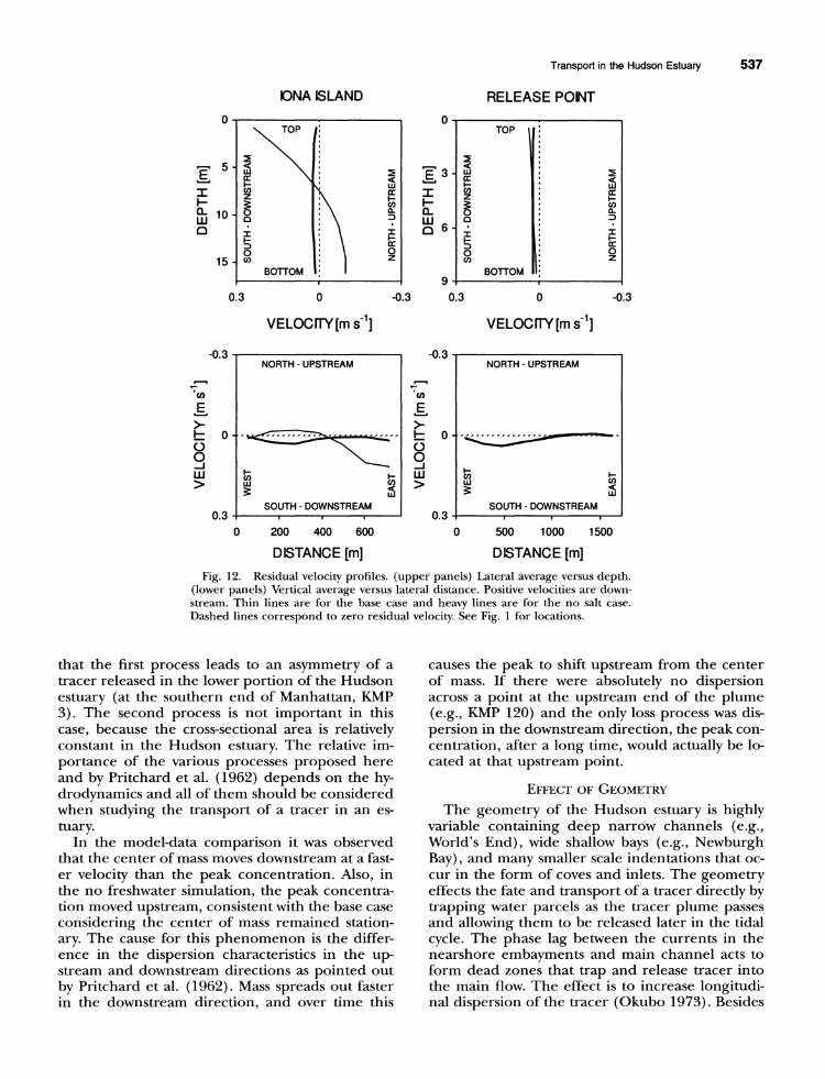
The presence of salt significantly changes the hydrodynamics at the downstream end of the plume. One effect is reduced vertical mixing. This is evident in the vertical SF6 concentration profiles in Fig. 11, where concentrations are normalized to that at the surface. As described in the model-data comparison, the base case shows a vertical stratifi- cation similar to the data. The no salt case is com- paratively well mixed throughout the water column. It shows a weak subsurface peak, which is due to tracer being removed from the surface to the atmosphere by gas transfer. The salt also affects the longitudinal velocities, as illustrated by vertical and transverse profiles of residual longitudinal velocities for the no salt and base cases presented in Fig. 12. At Iona Island, the velocities are significantly different between the two cases. The no salt case has relatively uniform vertical and horizontal dis- tributions of longitudinal velocities in the downstream direction. The base case has upstream velocities at the bottom and downstream velocities at the surface. This is the classical estuarine circulation described previously. Also, the lateral distribution of longitudinal velocities is more variable, with west bank velocities in the upstream direction.

I ? 1

r -T

z En

z o

.


E

z 0

cr z u. z

Co

10,000

1,000

100

10 60 120 60 80 100 120


Fig. 10. Longitudinal profiles of modeled surface SF6 concentration on August 4, 2001. Thin lines are for the base case and heavy lines are for various modifications (see text). Dashed lines correspond to the release location.

This is opposite to the typical Coriolis induced horizontal asymmetry, which would predict downstream movement on the west bank. The reason for this discrepancy is that the effect of the appar- ent Coriolis force is small compared to other factors (i.e., geometry). In Newburgh Bay, near the release point, the velocities of the two cases are similar. That is because at that location the salinity is close to zero in both cases.

SF6 CONCENTRATION [relative to surface]

I E w LU c]

0.5 1 1 0

10- f

20-

30 -

40- J

50

.5

Fig. 11. Vertical profiles of modeled (solid lines) and measured (points) SF6 concentrations at World's End on August 2, 2001. Concentrations are normalized to that at the surface. See Fig. 1 for station location. Thin line is for the base case and heavy line is for the no salt case.

We propose that three mechanisms related to the estuarine circulation at the downstream end of the plume are responsible for the asymmetric SF6 profile. The lesser vertical dispersion over the salt contributes to the asymmetric longitudinal concentration profile of surface concentrations, because less mass is lost to the deeper layers by vertical mixing. As pointed out by Pritchard (1954) and Fi- scher (1972), longitudinal dispersion is enhanced by lateral and vertical gradients in longitudinal velocities. The increased gradients in the presence of salt enhance longitudinal dispersion at the downstream end of the plume, contributing to the asymmetric longitudinal SF6 profile. The net downstream velocity in the surface layer, which corresponds to the concentration measurements, increases over the salt (compare base case in Fig. 12 panels). This accelerates the water carrying the tracer at the downstream end of the plume, stretching out the plume.

The above analysis demonstrates that the large- scale asymmetry is related to salinity and three mechanisms are proposed. It is interesting to note that those three mechanisms are different than the two proposed by Pritchard et al. (1962). They sug- gested that on the downstream side of estuaries increased tidal energy and cross sectional area can lead to an asymmetry. Using numerical and physical models of the Hudson estuary they showed

Transport in the Hudson Estuary

IONA ISLAND

TOP

? \ .

B \ |

z3 O 00~~~~~~~.

o c

0 Z

BOTTOM I

0

VELOCfTY[m s1]

RELEASE POINT

0

E 3- I- 0-

o 6-

9 -0.3 0.3

TOP

w 2 c' Z . z

o a

0 0

BOTTOM

0

VELOCITY [m s'1]

NORTH - UPSTREAM

3 I-

SOUTH - DOWNSTREAM

0 200 400 600

-0.3

EC) E

f 0-

0 uJ

0.3 C

DISTANCE [m]

NORTH - UPSTREAM

1) w 03

SOUTH - DOWNSTREAM

) 500 1000 1500

DISTANCE [m]

Fig. 12. Residual velocity profiles. (upper panels) Lateral average versus depth. (lower panels) Vertical average versus lateral distance. Positive velocities are downstream. Thin lines are for the base case and heavy lines are for the no salt case. Dashed lines correspond to zero residual velocity. See Fig. 1 for locations.

that the first process leads to an asymmetry of a tracer released in the lower portion of the Hudson estuary (at the southern end of Manhattan, KMP 3). The second process is not important in this case, because the cross-sectional area is relatively constant in the Hudson estuary. The relative importance of the various processes proposed here and by Pritchard et al. (1962) depends on the hydrodynamics and all of them should be considered when studying the transport of a tracer in an estuary.

In the model-data comparison it was observed that the center of mass moves downstream at a faster velocity than the peak concentration. Also, in the no freshwater simulation, the peak concentration moved upstream, consistent with the base case considering the center of mass remained station- ary. The cause for this phenomenon is the difference in the dispersion characteristics in the upstream and downstream directions as pointed out by Pritchard et al. (1962). Mass spreads out faster in the downstream direction, and over time this

causes the peak to shift upstream from the center of mass. If there were absolutely no dispersion across a point at the upstream end of the plume (e.g., KMP 120) and the only loss process was dispersion in the downstream direction, the peak concentration, after a long time, would actually be located at that upstream point.

EFFECT OF GEOMETRY

The geometry of the Hudson estuary is highly variable containing deep narrow channels (e.g., World's End), wide shallow bays (e.g., Newburgh Bay), and many smaller scale indentations that oc- cur in the form of coves and inlets. The geometry effects the fate and transport of a tracer directly by trapping water parcels as the tracer plume passes and allowing them to be released later in the tidal cycle. The phase lag between the currents in the nearshore embayments and main channel acts to form dead zones that trap and release tracer into the main flow. The effect is to increase longitudinal dispersion of the tracer (Okubo 1973). Besides

0

I

a. 10 0

15,

0.3 -0.3

-0.3

C.0

E

f_ 0

0 -J

0.3

1-

w

537


this tidal trapping, the overall dynamics of the circulation are also effected by the geometry, which can have indirect effects on tracer transport.

To investigate the effect of geometry on tracer transport the model grid was modified to a straight rectangular channel with dimensions based on those of the Hudson estuary covered by the model grid (width = 1.3 km, depth = 9 m). Other factors that introduce two-dimensional effects (tributary freshwater flow, wind, Coriolis force, and power plants) were kept as in the base case. The model predicts less overall spreading of the tracer plume illustrating that geometry irregularities contribute to the longitudinal dispersion (Fig. 10). The profile is relatively symmetric, which is a reflection of reduced salinity intrusion, consistent with the decreased longitudinal dispersion. For that reason it might be more appropriate to compare the straight channel case to the no salinity case. Al- though the profile is not perfectly smooth, there are no pronounced secondary peaks, which illustrates that those features are related to geometry irregularities. Small-scale embayments, like that near Wappinger Creek (KMP 106; Fig. 9) trap tracer mass leading to the secondary peaks in the longitudinal concentration profile.

ACKNOWLEDGMENTS

F. L. Hellweger, A. F. Blumberg, and H. Li were partially supported through research funding by HydroQual. A. F. Blumberg was also supported through the U.S. Department of Education Fund for the Improvement of Post Secondary Education. P. Schlosser, D. T. Ho, T. Caplow, U. Lall, and F. L. Hellweger are supported by a generous grant from the Dibner Fund and by the Columbia University Strategic Research Initiative. Two anonymous reviewers provided constructive criticism on the manuscript. This is Lamont-Doherty Earth Observatory contribution number LDEO 6609.

LITERATURE CITED

ABOOD, K. 1974. Circulation in the Hudson estuary. Annals of the New York Academy of Sciences 250:39-111.

BLUMBERG, A. F., D. J. DUNNING, H. LI, W. R. GEYER, AND D. HEIMBUCH. 2004. Use of a particle-tracking model for pre-

dicting entrainment at power plants on the Hudson River. Estuaries 27:515-526.

BLUMBERG, A. F., L. A. KHAN, AND J. P. ST. JOHN. 1999. Three- dimensional hydrodynamic model of New York harbor re- gion. Journal of Hydraulic Engineering 125:799-816.

BLUMBERG, A. F. AND B. N. KIM. 2000. Flow balances in St. An- drews Bay revealed through hydrodynamic simulations. Estu- aries 23:21-33.

BLUMBERG, A. F. AND G. L. MELLOR. 1987. A description of a three-dimensional coastal ocean circulation model, p. 1-16. In N. Heaps (ed.), Three-Dimensional Coastal Ocean Models. American Geophysical Union, Washington, D.C.

EZER, T. AND G. L. MELLOR. 2000. Sensitivity studies with the North Atlantic sigma coordinate Princeton Ocean Model. Dy- namics of Atmospheres and Oceans 32:185-208.

FISCHER, H. B. 1972. Mass transport mechanisms in partially stratified estuaries. Journal of Fluid Mechanics 53:671-687.

GEYER, R. W., J. H. TROWBRIDGE, AND M. M. BOWEN. 2000. The dynamics of a partially stratified estuary. Journal of Physical Oceanography 30:2035-2048.

Ho, D. T., P. SCHLOSSER, AND T. CAPLOW. 2002. Determination of longitudinal dispersion coefficient and net advection in the tidal Hudson River with a large-scale, high resolution SF6 tracer release experiment. Environmental Science and Technology 36: 3234-3241.

HUNKINS, K. 1981. Salt dispersion in the Hudson estuary. Journal of Physical Oceanography 11:729-738.

HYDROQUAL. 2001. A Primer for ECOMSED. Report Number HQI-EH&S0101. HydroQual, Mahwah, New Jersey.

KARA, A. B., P. A. ROCHFORD, AND H. E. HURLBURT. 2002. Air- sea flux estimates and the 1997-1998 ENSO event. Boundary- Layer Meteorology 103:439-458.

OKUBO, A. 1973. Effect of shoreline irregularities on streamwise dispersion in estuaries and other embayments. Netherlands Journal of Sea Research 6:213-224.

PRITCHARD, D. W. 1954. A study of salt balance in a coastal plain estuary. Journal of Marine Research 13:133-144.

PRITCHARD, D. W. 1969. Dispersion and flushing of pollutants in estuaries. Journal of the Hydraulics Division 95:115-124.

PRITCHARD, D. W., A. OKUBO, AND E. MEHR. 1962. A study of the movement and diffusion of an introduced contaminant in New York Harbor waters. Technical Report 31. Chesapeake Bay Institute, Johns Hopkins, Baltimore, Maryland.

SMAGORINSKY, J. 1963. General circulation experiments with the primitive equations, I. The basic experiment. Monthly Weather Review 91:99-164.

STEWARD, JR., H. B. 1958. Upstream bottom currents in New York Harbor. Science 127:1113-1115.

WANNINKHOF, R. 1992. Relationship between wind speed and gas exchange over the ocean. Journal of Geophysical Research 97: 7373-7382.

Received, July 25, 2003 Accepted, October 2, 2003

Transport in the Hudson Estuary: A Modeling Study of ...water.columbia.edu/files/2011/11/Lall2004Transport.pdf · Transport in the Hudson Estuary: A Modeling Study of Estuarine Circulation

Documents