Transmission Dynamics Modelling

IN DEGREE PROJECT VEHICLE ENGINEERING,SECOND CYCLE, 30 CREDITS

, STOCKHOLM SWEDEN 2018

Transmission Dynamics ModellingGear Whine Simulation Using AVL Excite

REZA MEHDIPOUR

KTH ROYAL INSTITUTE OF TECHNOLOGYSCHOOL OF ENGINEERING SCIENCES

ii

iii

Cover: The electrified transmission line used as a test object throughout this thesis work. The transmission line has been designed and developed by AVL Vicura in Trollhättan, Sweden.

iv

Abstract

Nowadays, increasing pressure from legislation and customer demands in the automotive industry are forcing manufacturers to produce greener vehicles with lower emissions and fuel consumption. As a result, electrified and hybrid vehicles are a growing popular alternative to traditional internal combustion engines (ICE). The noise from an electric vehicle comes mainly from contact between tyres and road, wind resistance and driveline. The noise emitted from the driveline is for the most part related to the gearbox. When developing a driveline, it is a factor of importance to estimate the noise radiating from the gearbox to achieve an acceptable design. Gears are used extensively in the driveline of electric vehicles. As the gears are in mesh, a main intrusive concern is known as gear whine noise. Gear whine noise is an undesired vibroacoustic phenomenon and is likely to originate through the gear contacts and be transferred through the mechanical components to the housing where the vibrations are converted into airborne and structure-borne noise. The gear whine noise originates primarily from the excitation coming from transmission error (TE). Transmission error is defined as the difference between the ideal smooth transfer of motion of a gear and what is in practice due to lack of smoothness. The main objective of this study is to simulate the vibrations generated by the gear whine noise in an electric powertrain line developed by AVL Vicura. The electric transmission used in this study provides only a fixed overall gear ratio, i.e. 9.59, under all operation conditions. It is assumed that the system is excited only by the transmission error and the mesh stiffness of the gear contacts. In order to perform NVH analysis under different operating conditions, a multibody dynamics model according to the AVL Excite program has been developed. The dynamic simulations are then compared with previous experimental measurements provided by AVL Vicura. Two validation criteria have been used to analyse the dynamic behaviour of the AVL Excite model: signal processing using the FFT method and comparison with the experimental measurements. The results from the AVL Excite model show that the FFT criterion is quite successful and all excitation frequencies are properly observed in FFT plots. Nevertheless, when it comes to the second criterion, as long as not all dynamic parameters of the system such as damping or stiffness coefficients are provided with certainty in the model, it is too difficult to investigate the accuracy of the AVL Excite model. Another investigation is a numerical design study to analyses how the damping coefficients influence the response. After reducing the damping parameters, the results show that the housing and bearings have the highest influence on the response. If more acceptable results are desired, future studies must be concentrated on these to obtain more acceptable damping values.

Keywords: Gear whine noise, transmission error (TE), mesh stiffness, gear mesh, multibody

dynamics simulation, reduction methods.

v

Sammanfattning

För närvarande tvingar ökat tryck från lagstiftning och kundkrav inom bilindustrin tillverkarna att producera grönare fordon med lägre utsläpp och bränsleförbrukning. Som ett resultat är elektrifierade och hybridfordon ett växande populärt alternativ till traditionella förbränningsmotorer (ICE). Bullret från ett elfordon kommer främst från kontakten mellan däck och väg, vindmotstånd och drivlinan. Bullret från drivlinan är i huvudsak relaterat till växellådan. Vid utveckling av en drivlina är det av betydelse att uppskatta bullret från växellådan för att uppnå en acceptabel design.

Utväxlingar används i stor utsträckning i elfordons drivlina. Eftersom kugghjulen är i kontakt uppstår ett huvudproblem som är känt som ett vinande ljud från kugghjulskontakten. Kugghjulsljud är ett oönskat vibro-akustiskt fenomen och uppstår sannolikt på grund av kugghjulkontakterna och överförs via de mekaniska komponenterna till växellådshuset där vibrationerna omvandlas till luftburet och strukturburet ljud. Kugghjulsljudet härstammar huvudsakligen från exciteringen som kommer från transmissionsfel (TE) i kugghjulskontakten. Överföringsfelet definieras som skillnaden mellan den ideala smidiga rörelseöverföringen hos kugghjulen och rörelsen som sker i verkligheten på grund av ojämnheter.

Huvudsyftet med denna studie är att simulera vibrationerna som genereras av kugghjulskontakterna i en elektrisk drivlina utvecklad av AVL Vicura. Den elektriska drivlinan som används i denna studie har endast ett fast utväxlingsförhållande, dvs 9,59, för alla driftsförhållanden. Det antas att systemet är exciterat endast av överföringsfelet och kugghjulens styvhet i kuggkontakterna. För att kunna utföra NVH-analys under olika driftsförhållanden har en stelkroppsdynamikmodell utvecklats med hjälp av programmet AVL Excite. De dynamiska simuleringarna jämförs sedan med tidigare experimentella mätningar som tillhandahålls av AVL Vicura.

Två valideringskriterier har använts för att analysera det dynamiska beteendet hos AVL Excite-modellen: signalbehandling med FFT-metoden och jämförelse med experimentella mätningar. Resultaten från AVL Excite-modellen visar att FFT-kriteriet är ganska framgångsrikt och alla excitationsfrekvenser observeras korrekt i FFT-diagrammen. Men när det gäller det andra kriteriet, så länge som inte alla dynamiska parametrar i systemet, såsom dämpnings- eller styvhetskoefficienter, är tillförlitliga i modellen, är det för svårt att undersöka exaktheten hos AVL Excite-modellen.

En annan undersökning som utförts är en numerisk designstudie för att analysera hur dämpningskoefficienterna påverkar responsen. Efter minskning av dämpningsparametrarna visar resultaten att växellådshus och lager har störst inflytande på resultatet. Om mer acceptabla resultat är önskvärda måste framtida studier koncentreras på dessa parametrar för att uppnå mer acceptabla dämpningsvärden.

Nyckelord: Kugghjulsljud, transmissionsfel (TE), kuggstyvhet, kuggingrepp, stelkroppssimulering, reduktionsmetoder.

vi

I dedicate this thesis work to all birds in Trollhättan. During this work, they have inspired me to learn much more about freedom. They do not care the borders built among humans and break the limitations by flying over the borders.

vii

Preface This thesis is a part of the master degree at KTH Royal Institute of Technology, and has been carried out in collaboration with AVL Vicura in Trollhättan, Sweden.

Acknowledgements I would like to express my sincere gratitude to my supervisor and examiner, Martin Johansson and Lars Drugge, for their great support throughout the whole project. This work wouldn’t have been possible without their immense support, tack så mycket Martin and Lars. I also acknowledge the contribution of all AVL Vicura’s simulation engineers for taking their time to help me through the project, especially Farhan Khan and Peyman Jafarian. I would also like to thank Mehdi Mehrgou and Dieter Wallner at AVL in Graz, Austria and Samuel Brauer at AVL in Södertälje, Sweden and Pouyan Alimouri who greatly helped me throughout the modelling and simulation. Finally, I sincerely appreciate Jamie Rinder for his continuous support to edit the report. Trollhättan, autumn 2017

Reza MehdiPour

viii

Table of Contents

1 Introduction 1

1.1 Objective .............................................................................................................................. 2

1.2 Description of the examined powertrain ............................................................................... 2

2 Theory 3

2.1 Gear whine noise and transmission error .............................................................................. 3

2.1.1 Sources of Transmission Error (TE) .............................................................................. 4

2.1.2 Types of transmission error ............................................................................................ 5

2.1.2.1 Manufacturing Transmission Error (MTE) .................................................................. 5

2.1.2.2 Static Transmission Error (STE) ................................................................................. 5

2.1.2.3 Dynamic Transmission Error (DTE) ........................................................................... 5

2.1.3 Gear dynamic modelling ................................................................................................ 6

2.1.3.1 Gear contact models.................................................................................................... 6

2.2 Helical involute gear geometry .............................................................................................. 8

2.2.1 Gear-tooth action ........................................................................................................... 8

2.2.2 Forces in helical gears................................................................................................... 10

2.3 Vibration theory .................................................................................................................. 11

2.3.1 Free damped systems ................................................................................................... 12

2.3.2 Forced damped systems ............................................................................................... 13

2.3.3 Modal analysis method ................................................................................................. 13

2.3.4 Torsional vibration ....................................................................................................... 14

2.3.5 N-DoF systems ............................................................................................................ 15

2.4 Multibody system dynamics ................................................................................................ 15

2.4.1 AVL Excite power unit ................................................................................................ 16

2.4.2 AVL Excite power unit component modelling ............................................................. 16

2.4.2.1 Advanced Cylindrical Gear Joint (ACYG) ................................................................. 16

2.4.2.1.1.1 Pre-calculations .................................................................................................... 18

2.4.2.1.1.2 Detection of contact ............................................................................................ 18

2.4.2.1.1.3 Constitution of the deformation field ................................................................... 19

2.4.2.1.1.4 Computation of normal forces ............................................................................. 20

2.4.2.2 Bearing modelling ...................................................................................................... 21

2.5 Sub-structuring concept ...................................................................................................... 23

2.5.1 Craig-Bampton method ................................................................................................ 24

ix

2.5.1.1 The fixed-interface vibration modes .......................................................................... 24

2.5.1.2 Constraint modes ...................................................................................................... 25

2.5.1.3 Reduction matrix ....................................................................................................... 25

2.6 Rayleigh damping ................................................................................................................ 26

2.7 Fast Fourier Transform (FFT) ............................................................................................ 26

2.8 Gear-mesh frequency analysis ............................................................................................. 27

3 Methods 29

3.1 Dynamic model analysis description ................................................................................... 29

3.2 Simulation software ............................................................................................................ 31

3.3 Layout of the AVL excite model ......................................................................................... 31

3.4 Experimental test ................................................................................................................ 32

3.5 Joints .................................................................................................................................. 34

3.5.1 Advanced Cylindrical Gear Joint (ACYG) .................................................................... 34

3.5.2 Deep drove bearing (DGBB) ....................................................................................... 36

3.5.3 ROTX joints ................................................................................................................ 37

3.6 Bodies ................................................................................................................................. 37

3.6.1 Input shaft ................................................................................................................... 38

3.6.2 Main shaft .................................................................................................................... 39

3.6.3 Differential ................................................................................................................... 39

3.6.4 Housing ....................................................................................................................... 41

3.7 Engine mounts ................................................................................................................... 43

3.8 Simulation methodology and boundary conditions.............................................................. 43

4 Results 45

4.1 The simulation results from the AVL Excite model ............................................................ 46

4.1.1 Analysis and comparison .............................................................................................. 47

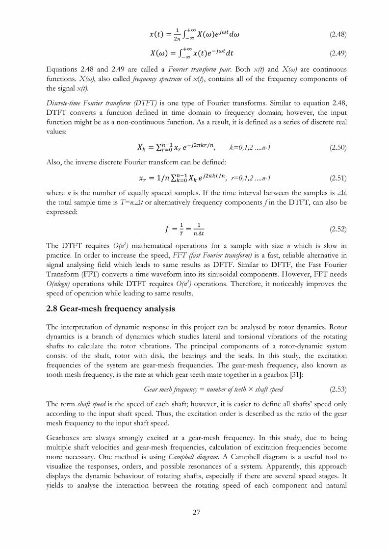
4.1.2 Campbell diagram ........................................................................................................ 52

4.2 FFT analysis on different range of cycles ............................................................................ 54

4.3 Experimental tests comparison ........................................................................................... 55

4.4 Experimental design analysis ............................................................................................... 56

5 Discussion and conclusions 61

5.1 Discussion .......................................................................................................................... 61

5.1.1 Calculated dynamic response error ............................................................................... 61

5.1.2 Dynamic response of the transmission housing ............................................................ 62

5.1.3 Experimental design analysis ........................................................................................ 62

x

5.2 Conclusions ........................................................................................................................ 63

5.3 Future work ........................................................................................................................ 64

References 66

xi

Nomenclature

c Damping coefficient cd Center distance cm Mesh damping

CR Contact ratio e(t) Excitation Fa Axial force fm Mesh frequency

fmax Maximum frequency Fn Normal force Ft Transverse force i Gear ratio k Stiffness km Mesh stiffness kt Torsional stiffness M Torque m Mass n Number of samples pb Base pitch r Pitch radius rb Base radius t time T Total time Tm Time period of mesh cycle

TEang Angular transmission error TElin Linear transmission error

x Displacement z Number of gear teeth βb Helix angle θ Angular position φ Pressure angle ω Angular velocity

1

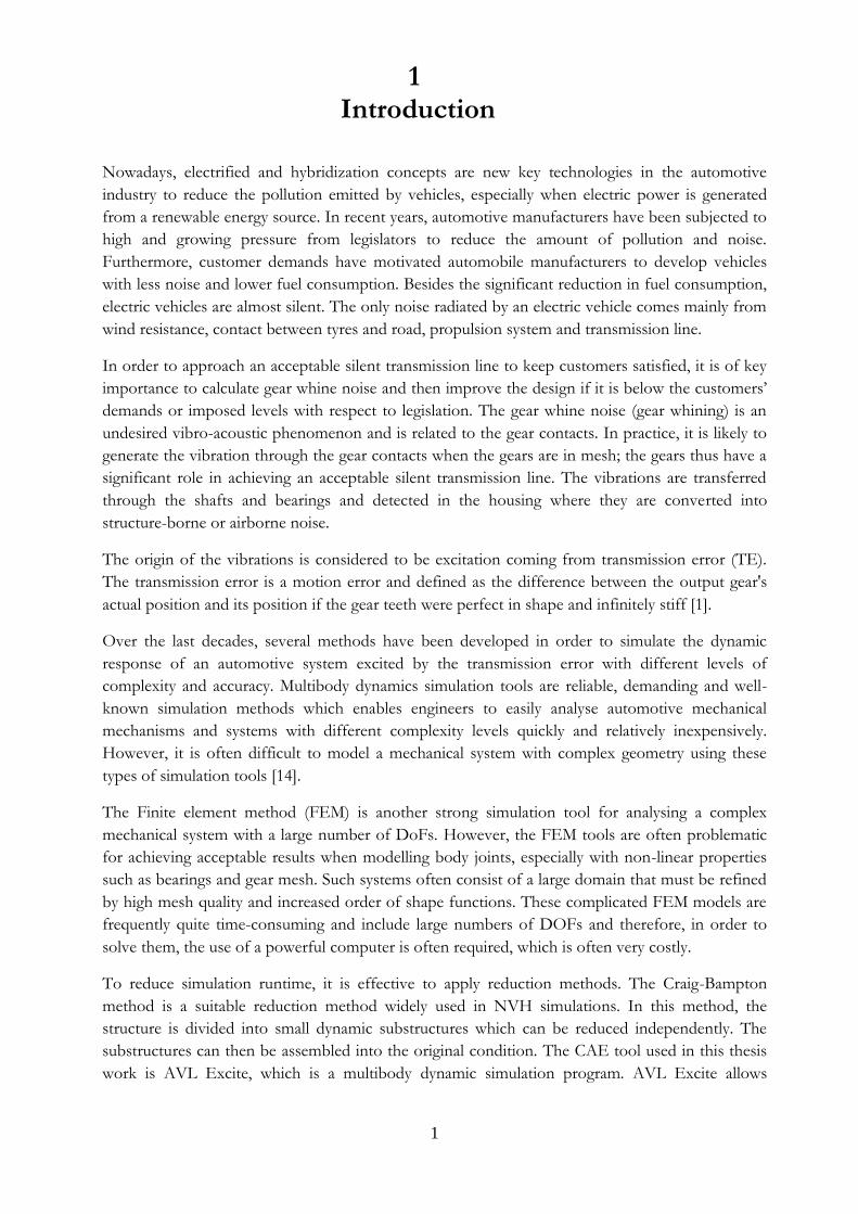
1 Introduction

Nowadays, electrified and hybridization concepts are new key technologies in the automotive

industry to reduce the pollution emitted by vehicles, especially when electric power is generated

from a renewable energy source. In recent years, automotive manufacturers have been subjected to

high and growing pressure from legislators to reduce the amount of pollution and noise.

Furthermore, customer demands have motivated automobile manufacturers to develop vehicles

with less noise and lower fuel consumption. Besides the significant reduction in fuel consumption,

electric vehicles are almost silent. The only noise radiated by an electric vehicle comes mainly from

wind resistance, contact between tyres and road, propulsion system and transmission line.

In order to approach an acceptable silent transmission line to keep customers satisfied, it is of key

importance to calculate gear whine noise and then improve the design if it is below the customers’

demands or imposed levels with respect to legislation. The gear whine noise (gear whining) is an

undesired vibro-acoustic phenomenon and is related to the gear contacts. In practice, it is likely to

generate the vibration through the gear contacts when the gears are in mesh; the gears thus have a

significant role in achieving an acceptable silent transmission line. The vibrations are transferred

through the shafts and bearings and detected in the housing where they are converted into

structure-borne or airborne noise.

The origin of the vibrations is considered to be excitation coming from transmission error (TE).

The transmission error is a motion error and defined as the difference between the output gear's

actual position and its position if the gear teeth were perfect in shape and infinitely stiff [1].

Over the last decades, several methods have been developed in order to simulate the dynamic

response of an automotive system excited by the transmission error with different levels of

complexity and accuracy. Multibody dynamics simulation tools are reliable, demanding and well-

known simulation methods which enables engineers to easily analyse automotive mechanical

mechanisms and systems with different complexity levels quickly and relatively inexpensively.

However, it is often difficult to model a mechanical system with complex geometry using these

types of simulation tools [14].

The Finite element method (FEM) is another strong simulation tool for analysing a complex

mechanical system with a large number of DoFs. However, the FEM tools are often problematic

for achieving acceptable results when modelling body joints, especially with non-linear properties

such as bearings and gear mesh. Such systems often consist of a large domain that must be refined

by high mesh quality and increased order of shape functions. These complicated FEM models are

frequently quite time-consuming and include large numbers of DOFs and therefore, in order to

solve them, the use of a powerful computer is often required, which is often very costly.

To reduce simulation runtime, it is effective to apply reduction methods. The Craig-Bampton

method is a suitable reduction method widely used in NVH simulations. In this method, the

structure is divided into small dynamic substructures which can be reduced independently. The

substructures can then be assembled into the original condition. The CAE tool used in this thesis

work is AVL Excite, which is a multibody dynamic simulation program. AVL Excite allows

2

engineers to simulate the dynamic behaviour of joints, such as bearings and gears, with acceptable

results. AVL Excite can also be easily linked with FEM tools like Abaqus.

1.1 Objective This thesis work has been performed in collaboration with AVL Vicura in Trollhättan, Sweden.

AVL Excite simulates the vibration responses originated by the gear whine noise in an electric

gearbox developed at AVL Vicura. It is assumed that the vibration originated in the system is

primarily excited by the transmission error. There are two validation criteria to investigate the

accuracy of the model created in AVL Excite. The first criterion is the FFT method and the other

is to compare with previous experimental measurements provided by AVL Vicura.

1.2 Description of the examined powertrain

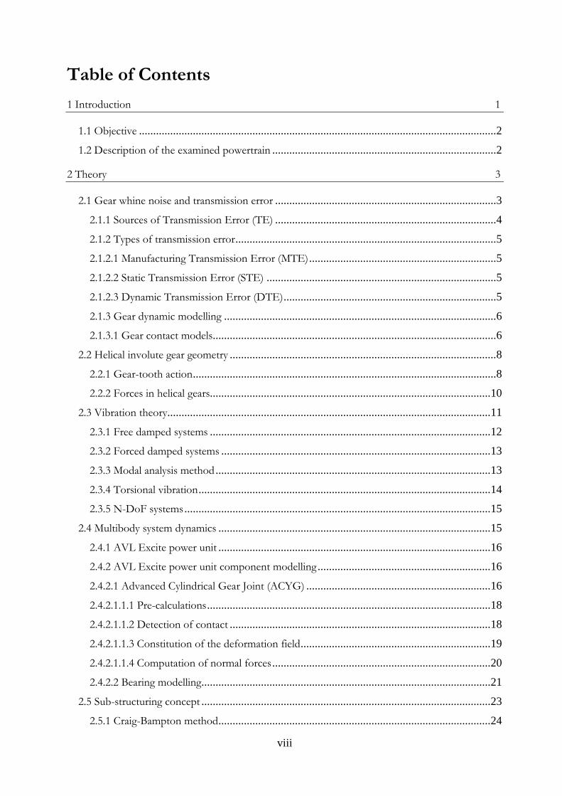
The electric transmission used in this study provides only a fixed overall gear ratio, i.e. 9.59, during

all operation conditions. The function of the transmission line is to deliver power from an electric

motor attached to the gearbox to the wheels. Since the overall gear ratio is larger than 1, the torque

is therefore increased while the speed is reduced.

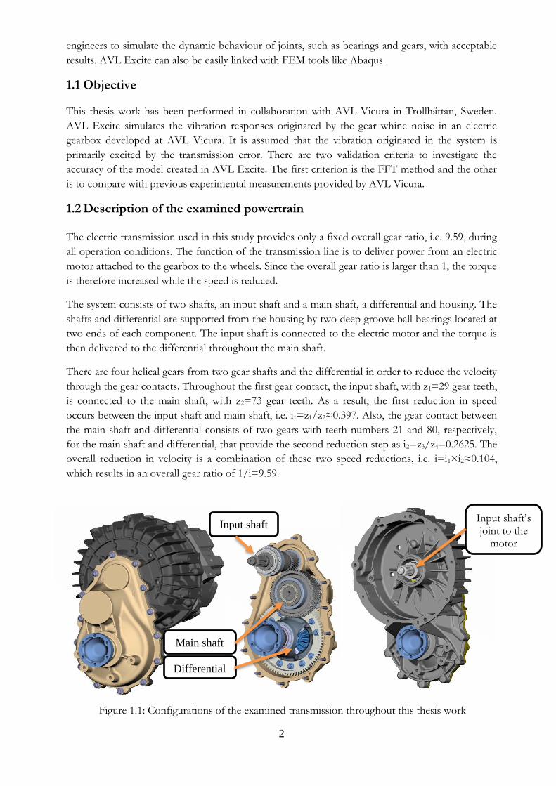
The system consists of two shafts, an input shaft and a main shaft, a differential and housing. The

shafts and differential are supported from the housing by two deep groove ball bearings located at

two ends of each component. The input shaft is connected to the electric motor and the torque is

then delivered to the differential throughout the main shaft.

There are four helical gears from two gear shafts and the differential in order to reduce the velocity

through the gear contacts. Throughout the first gear contact, the input shaft, with z1=29 gear teeth,

is connected to the main shaft, with z2=73 gear teeth. As a result, the first reduction in speed

occurs between the input shaft and main shaft, i.e. i1=z1/z2≈0.397. Also, the gear contact between

the main shaft and differential consists of two gears with teeth numbers 21 and 80, respectively,

for the main shaft and differential, that provide the second reduction step as i2=z3/z4=0.2625. The

overall reduction in velocity is a combination of these two speed reductions, i.e. i=i1×i2≈0.104,

which results in an overall gear ratio of 1/i=9.59.

Figure 1.1: Configurations of the examined transmission throughout this thesis work

Input shaft Input shaft’s joint to the

motor

Main shaft

Differential

3

2

Theory The purpose of this chapter is to present the theory behind this study. It starts with a description

of the gear whine phenomena, introduces the terminology of the helical gears and the

characteristics of the involute gears. It also describes different gear contact models and the forces

interacting between the gears when they are in mesh. Since the concepts behind this study are

fundamentally associated with NVH, the theory of vibration is also briefly explained. The last

section extensively explains the multibody dynamic simulation and concludes with the Fast Fourier

Transform (FFT) and the gear-mesh frequency analysis.

2.1 Gear whine noise and transmission error In power transmission design, gear whine noise is a common annoying vibrational phenomenon. It

is a tonal sound emitted from the gears as they mesh. In principle, the gear whine noise is a

noticeable challenge for NVH engineers and must be reduced below an acceptable level. The

acceptable level is defined according to automotive legislation and the satisfaction of the

customers. Due to the behaviour of the noise being periodic, it can be considered to be tonal

noise. The frequency of the noise is the same as the frequency of the gear mesh and its multiples.

Over the past decades, when ICE vehicles were attractive, gear whine noise has not been

considered to be a very important annoying problem. Since other noises that affected the

passengers and drivers in the vehicle cabin were more annoying and has a greater effect, as a result

reduction of the gear whine noise was not a priority for NVH engineers. Nowadays, although ICE

manufacturers are paying more attention to reducing the noise arising from the gear whine sources,

gear whining is still a major annoying problem.

After the appearance of electric and hybrid vehicles with low propulsion noise, it is of key

importance to reduce the gear whine below an acceptable level. The vibration can be transmitted

through the mechanical components such as shafts and bearings. The housing of the gearbox is

then excited and the vibration is converted into airborne and structure-borne noise. The vibration

from the engine mounts of the housing can also be transferred to the chassis and sensed by people

inside the vehicle cabin [2].

Ideally, if the gears operate under perfect conditions, they generate much lower noise. However, in

reality, the manufacturing tolerance and misalignment of the shafts may cause vibration. The

transmission error is a primary source of generation of gear whine noise. The transmission error

can be defined as “the difference between the actual position of the output gear and the position it

would occupy if the gear drive were perfect” [1].

If a gear pair is assumed completely rigid, with perfectly uniform involute teeth profiles, they will

transmit exactly smooth angular motion. However, in practice the gears are elastic and they can not

meet these assumed conditions and, thus, the pair of meshing gears can not transmit a uniform

angular motion. Consequently, transmission error is inevitable. Any deviation between the

theoretical angular motion and the actual angular velocity can be attributed to the transmission

error [2].

4

The transmission error is greatly dependent on the transmission torque which is transferred by the

gear pair. As a larger torque is applied on the gear pair, a greater deformation can appear on the

gear teeth that will lead to a larger difference between the actual and theoretical angular position of

the gears, or larger transmission error. It can obviously be easily accepted that it is desirable to

minimize the transmission error. More specifically, since the transmission error is a source of noise

generation, NVH engineers try to obtain a transmission error with a low variation.

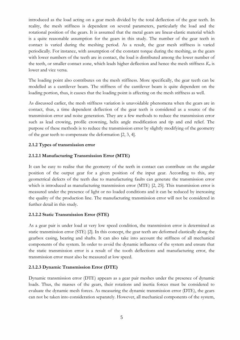
As figure 2.1 shows, due to the definition of the transmission error, it can be formulated as the

difference between the theoretical and actual angular displacement of two gears. Hence, it can be

written in terms of the angular positions of gear 1 and 2, θ1 and θ2, and their corresponding angular

velocities, N1 and N2

𝑇𝐸(𝜔) = 𝜃1(𝜔) −𝑁2

𝑁1𝜃2(𝜔) (2.1)

Or, it can also be written according to the corresponding base radii, rb1 and rb2

𝑇𝐸(𝜔) = 𝜃1(𝜔) −𝑟𝑏2

𝑟𝑏1𝜃2(𝜔) (2.2)

Figure 2.1: Geometrical illustration of transmission error

2.1.1 Sources of Transmission Error (TE) As previously discussed, the transmission error and mesh stiffness are often the main sources of

the noise generation as the gears are in contact. Consequently, minimizing the transmission error is

important to reduce the noise generation. In order to approach this goal, the main sources of the

transmission error must be detected. Many researchers describe that the main sources of the

transmission error are associated with the geometry, deflection, dynamics of the gears and variation

of applying loads. The geometry error is due to the practical assembly and manufacturing.

Misalignment of the shafts and gears during the assembly can also contribute to generate the

transmission error [2].

Mesh stiffness Km variation highly contributes on the transmission error. The loading on a gear

mesh is in the form of bending and contact between the teeth. Thus, the mesh stiffness Km can be

5

introduced as the load acting on a gear mesh divided by the total deflection of the gear teeth. In

reality, the mesh stiffness is dependent on several parameters, particularly the load and the

rotational position of the gears. It is assumed that the metal gears are linear-elastic material which

is a quite reasonable assumption for the gears in this study. The number of the gear teeth in

contact is varied during the meshing period. As a result, the gear mesh stiffness is varied

periodically. For instance, with assumption of the constant torque during the meshing, as the gears

with lower numbers of the teeth are in contact, the load is distributed among the lower number of

the teeth, or smaller contact zone, which leads higher deflection and hence the mesh stiffness Km is

lower and vice versa.

The loading point also contributes on the mesh stiffness. More specifically, the gear teeth can be

modelled as a cantilever beam. The stiffness of the cantilever beam is quite dependent on the

loading portion, thus, it causes that the loading point is affecting on the mesh stiffness as well.

As discussed earlier, the mesh stiffness variation is unavoidable phenomena when the gears are in

contact, thus, a time dependent deflection of the gear teeth is considered as a source of the

transmission error and noise generation. They are a few methods to reduce the transmission error

such as lead crowing, profile crowning, helix angle modification and tip and end relief. The

purpose of these methods is to reduce the transmission error by slightly modifying of the geometry

of the gear teeth to compensate the deformation [2, 3, 4].

2.1.2 Types of transmission error 2.1.2.1 Manufacturing Transmission Error (MTE) It can be easy to realise that the geometry of the teeth in contact can contribute on the angular

position of the output gear for a given position of the input gear. According to this, any

geometrical defects of the teeth due to manufacturing faults can generate the transmission error

which is introduced as manufacturing transmission error (MTE) [2, 25]. This transmission error is

measured under the presence of light or no loaded conditions and it can be reduced by increasing

the quality of the production line. The manufacturing transmission error will not be considered in

further detail in this study.

2.1.2.2 Static Transmission Error (STE) As a gear pair is under load at very low speed condition, the transmission error is determined as

static transmission error (STE) [2]. In this concept, the gear teeth are deformed elastically along the

gearbox casing, bearing and shafts. It can also take into account the stiffness of all mechanical

components of the system. In order to avoid the dynamic influence of the system and ensure that

the static transmission error is a result of the tooth deflections and manufacturing error, the

transmission error must also be measured at low speed.

2.1.2.3 Dynamic Transmission Error (DTE) Dynamic transmission error (DTE) appears as a gear pair meshes under the presence of dynamic

loads. Thus, the masses of the gears, their rotations and inertia forces must be considered to

evaluate the dynamic mesh forces. As measuring the dynamic transmission error (DTE), the gears

can not be taken into consideration separately. However, all mechanical components of the system,

6

such as the shafts, gears and bearings must be placed in the housing because the dynamical

properties of all components are very important and influence each other.

The static transmission error is the source of the excitation for the dynamic transmission error.

Since the dynamic transmission error is dependent on the speed, thus, it can be explained by

multiplying the static transmission error by adding a transfer function. In the recent decades, plenty

of conducted research has been performed to model the dynamic transmission error using

methods such as a simple dynamic factor model, compliance tooth model, torsional model and

geared rotor dynamic model [2, 5, 26].

2.1.3 Gear dynamic modelling This section deals with different proposed models developed to analyse the dynamic behaviour of

the gear meshing.

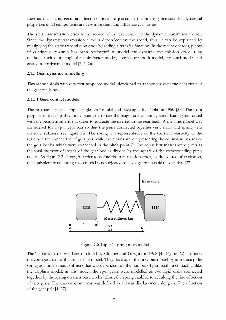
2.1.3.1 Gear contact models The first concept is a simple, single DoF model and developed by Tuplin in 1950 [27]. The main

purpose to develop this model was to estimate the magnitude of the dynamic loading associated

with the geometrical error in order to evaluate the stresses in the gear teeth. A dynamic model was

considered for a spur gear pair so that the gears connected together via a mass and spring with

constant stiffness, see figure 2.2. The spring was representative of the torsional elasticity of the

system in the connection of gear pair while the masses were representing the equivalent masses of

the gear bodies which were connected in the pitch point P. The equivalent masses were given as

the total moment of inertia of the gear bodies divided by the square of the corresponding pitch

radius. As figure 2.2 shows, in order to define the transmission error, as the source of excitation,

the equivalent mass-spring-mass model was subjected to a wedge or sinusoidal excitation [27].

Figure 2.2: Tuplin’s spring-mass model

The Tuplin’s model was later modified by Cloutier and Gregory in 1962 [4]. Figure 2.2 illustrates

the configuration of this single 1-D model. They developed the previous model by introducing the

spring as a time variant stiffness that was dependent on the number of gear teeth in contact. Unlike

the Tuplin’s model, in this model, the spur gears were modelled as two rigid disks connected

together by the spring on their base circles. Thus, the spring enabled to act along the line of action

of two gears. The transmission error was defined as a linear displacement along the line of action

of the gear pair [4, 27].

7

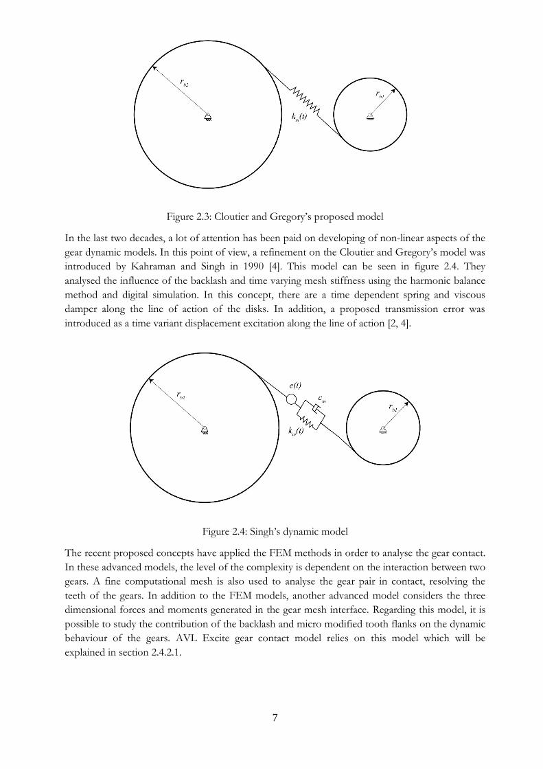
Figure 2.3: Cloutier and Gregory’s proposed model

In the last two decades, a lot of attention has been paid on developing of non-linear aspects of the

gear dynamic models. In this point of view, a refinement on the Cloutier and Gregory’s model was

introduced by Kahraman and Singh in 1990 [4]. This model can be seen in figure 2.4. They

analysed the influence of the backlash and time varying mesh stiffness using the harmonic balance

method and digital simulation. In this concept, there are a time dependent spring and viscous

damper along the line of action of the disks. In addition, a proposed transmission error was

introduced as a time variant displacement excitation along the line of action [2, 4].

Figure 2.4: Singh’s dynamic model

The recent proposed concepts have applied the FEM methods in order to analyse the gear contact.

In these advanced models, the level of the complexity is dependent on the interaction between two

gears. A fine computational mesh is also used to analyse the gear pair in contact, resolving the

teeth of the gears. In addition to the FEM models, another advanced model considers the three

dimensional forces and moments generated in the gear mesh interface. Regarding this model, it is

possible to study the contribution of the backlash and micro modified tooth flanks on the dynamic

behaviour of the gears. AVL Excite gear contact model relies on this model which will be

explained in section 2.4.2.1.

8

2.2 Helical involute gear geometry Gears have a long history dating back since human began making primary machinery devices. A

gear is a rotating machine which its primary function is to transfer the torque between the shafts

while the speed ratio can be held constant. There are several types of gear configurations such as

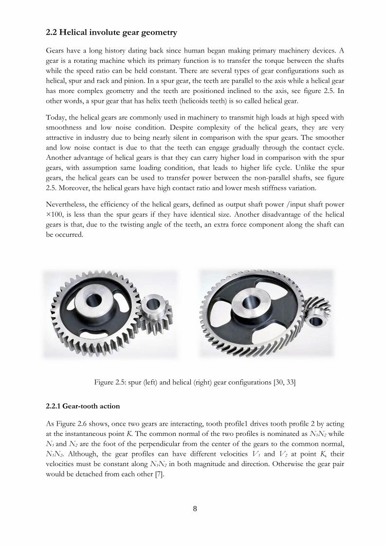
helical, spur and rack and pinion. In a spur gear, the teeth are parallel to the axis while a helical gear

has more complex geometry and the teeth are positioned inclined to the axis, see figure 2.5. In

other words, a spur gear that has helix teeth (helicoids teeth) is so called helical gear.

Today, the helical gears are commonly used in machinery to transmit high loads at high speed with

smoothness and low noise condition. Despite complexity of the helical gears, they are very

attractive in industry due to being nearly silent in comparison with the spur gears. The smoother

and low noise contact is due to that the teeth can engage gradually through the contact cycle.

Another advantage of helical gears is that they can carry higher load in comparison with the spur

gears, with assumption same loading condition, that leads to higher life cycle. Unlike the spur

gears, the helical gears can be used to transfer power between the non-parallel shafts, see figure

2.5. Moreover, the helical gears have high contact ratio and lower mesh stiffness variation.

Nevertheless, the efficiency of the helical gears, defined as output shaft power /input shaft power

×100, is less than the spur gears if they have identical size. Another disadvantage of the helical

gears is that, due to the twisting angle of the teeth, an extra force component along the shaft can

be occurred.

Figure 2.5: spur (left) and helical (right) gear configurations [30, 33]

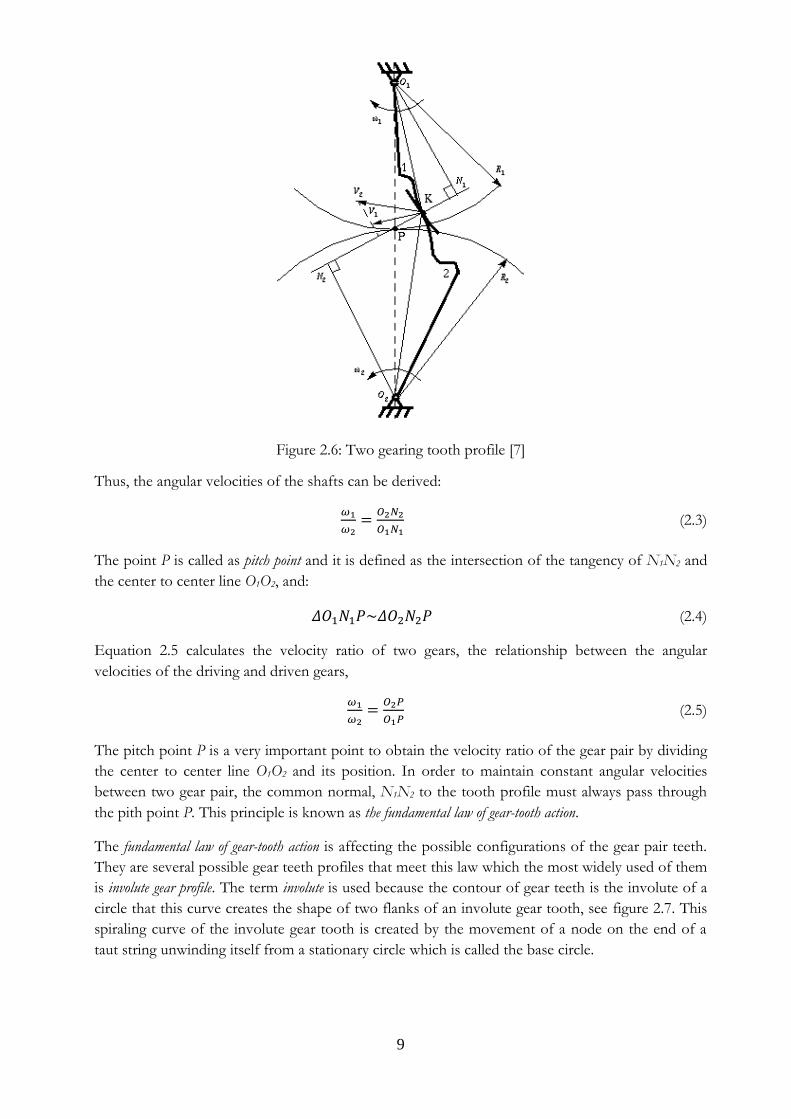
2.2.1 Gear-tooth action As Figure 2.6 shows, once two gears are interacting, tooth profile1 drives tooth profile 2 by acting

at the instantaneous point K. The common normal of the two profiles is nominated as N1N2 while

N1 and N2 are the foot of the perpendicular from the center of the gears to the common normal,

N1N2. Although, the gear profiles can have different velocities V1 and V2 at point K, their

velocities must be constant along N1N2 in both magnitude and direction. Otherwise the gear pair

would be detached from each other [7].

9

Figure 2.6: Two gearing tooth profile [7]

Thus, the angular velocities of the shafts can be derived:

𝜔1

𝜔2=

𝑂2𝑁2

𝑂1𝑁1 (2.3)

The point P is called as pitch point and it is defined as the intersection of the tangency of N1N2 and

the center to center line O1O2, and:

𝛥𝑂1𝑁1𝑃~𝛥𝑂2𝑁2𝑃 (2.4)

Equation 2.5 calculates the velocity ratio of two gears, the relationship between the angular

velocities of the driving and driven gears,

𝜔1

𝜔2=

𝑂2𝑃

𝑂1𝑃 (2.5)

The pitch point P is a very important point to obtain the velocity ratio of the gear pair by dividing

the center to center line O1O2 and its position. In order to maintain constant angular velocities

between two gear pair, the common normal, N1N2 to the tooth profile must always pass through

the pith point P. This principle is known as the fundamental law of gear-tooth action.

The fundamental law of gear-tooth action is affecting the possible configurations of the gear pair teeth.

They are several possible gear teeth profiles that meet this law which the most widely used of them

is involute gear profile. The term involute is used because the contour of gear teeth is the involute of a

circle that this curve creates the shape of two flanks of an involute gear tooth, see figure 2.7. This

spiraling curve of the involute gear tooth is created by the movement of a node on the end of a

taut string unwinding itself from a stationary circle which is called the base circle.

10

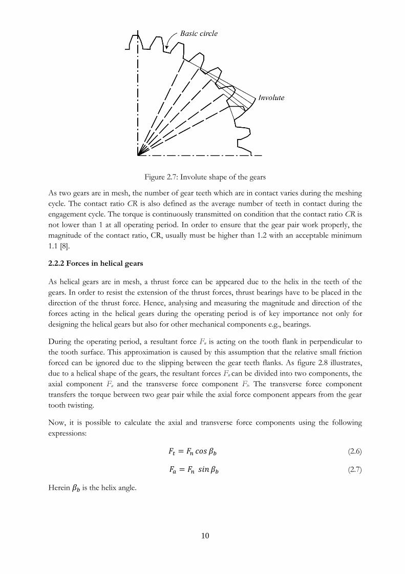
Figure 2.7: Involute shape of the gears

As two gears are in mesh, the number of gear teeth which are in contact varies during the meshing

cycle. The contact ratio CR is also defined as the average number of teeth in contact during the

engagement cycle. The torque is continuously transmitted on condition that the contact ratio CR is

not lower than 1 at all operating period. In order to ensure that the gear pair work properly, the

magnitude of the contact ratio, CR, usually must be higher than 1.2 with an acceptable minimum

1.1 [8].

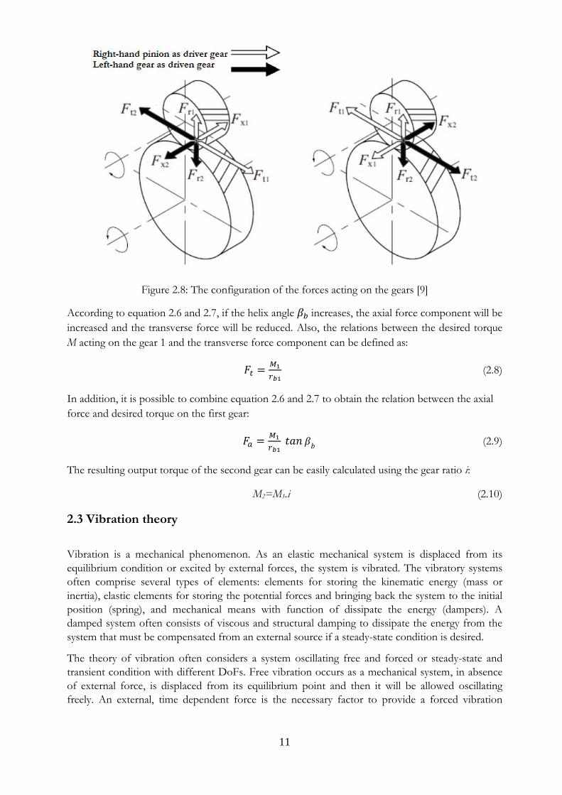
2.2.2 Forces in helical gears As helical gears are in mesh, a thrust force can be appeared due to the helix in the teeth of the

gears. In order to resist the extension of the thrust forces, thrust bearings have to be placed in the

direction of the thrust force. Hence, analysing and measuring the magnitude and direction of the

forces acting in the helical gears during the operating period is of key importance not only for

designing the helical gears but also for other mechanical components e.g., bearings.

During the operating period, a resultant force Fn is acting on the tooth flank in perpendicular to

the tooth surface. This approximation is caused by this assumption that the relative small friction

forced can be ignored due to the slipping between the gear teeth flanks. As figure 2.8 illustrates,

due to a helical shape of the gears, the resultant forces Fn can be divided into two components, the

axial component Fa and the transverse force component Ft. The transverse force component

transfers the torque between two gear pair while the axial force component appears from the gear

tooth twisting.

Now, it is possible to calculate the axial and transverse force components using the following

expressions:

𝐹𝑡 = 𝐹𝑛 𝑐𝑜𝑠 𝛽𝑏 (2.6)

𝐹𝑎 = 𝐹𝑛 𝑠𝑖𝑛 𝛽𝑏 (2.7)

Herein 𝛽𝑏 is the helix angle.

11

Figure 2.8: The configuration of the forces acting on the gears [9]

According to equation 2.6 and 2.7, if the helix angle 𝛽𝑏 increases, the axial force component will be

increased and the transverse force will be reduced. Also, the relations between the desired torque

M acting on the gear 1 and the transverse force component can be defined as:

𝐹𝑡 =𝑀1

𝑟𝑏1 (2.8)

In addition, it is possible to combine equation 2.6 and 2.7 to obtain the relation between the axial

force and desired torque on the first gear:

𝐹𝑎 =𝑀1

𝑟𝑏1 𝑡𝑎𝑛 𝛽

𝑏 (2.9)

The resulting output torque of the second gear can be easily calculated using the gear ratio i:

M2=M1.i (2.10)

2.3 Vibration theory

Vibration is a mechanical phenomenon. As an elastic mechanical system is displaced from its

equilibrium condition or excited by external forces, the system is vibrated. The vibratory systems

often comprise several types of elements: elements for storing the kinematic energy (mass or

inertia), elastic elements for storing the potential forces and bringing back the system to the initial

position (spring), and mechanical means with function of dissipate the energy (dampers). A

damped system often consists of viscous and structural damping to dissipate the energy from the

system that must be compensated from an external source if a steady-state condition is desired.

The theory of vibration often considers a system oscillating free and forced or steady-state and

transient condition with different DoFs. Free vibration occurs as a mechanical system, in absence

of external force, is displaced from its equilibrium point and then it will be allowed oscillating

freely. An external, time dependent force is the necessary factor to provide a forced vibration

12

system. The external force can have different features such as periodic, steady-state and transient

or random.

If a system is forced by a harmonic force, the response of the system can be harmonic with same

frequency of the acting force; however, the amplitude could be a function of characteristics of the

system. If the external frequency is equal to the natural frequency of the system, the system will be

critically vibrated and the amplitude increases. This undesired phenomenon is so called resonance.

The number of natural frequencies of a system is equal to its DoFs. For instance, for a real

continuous system, the number of DoFs is infinite that leads to infinite number of natural

frequencies.

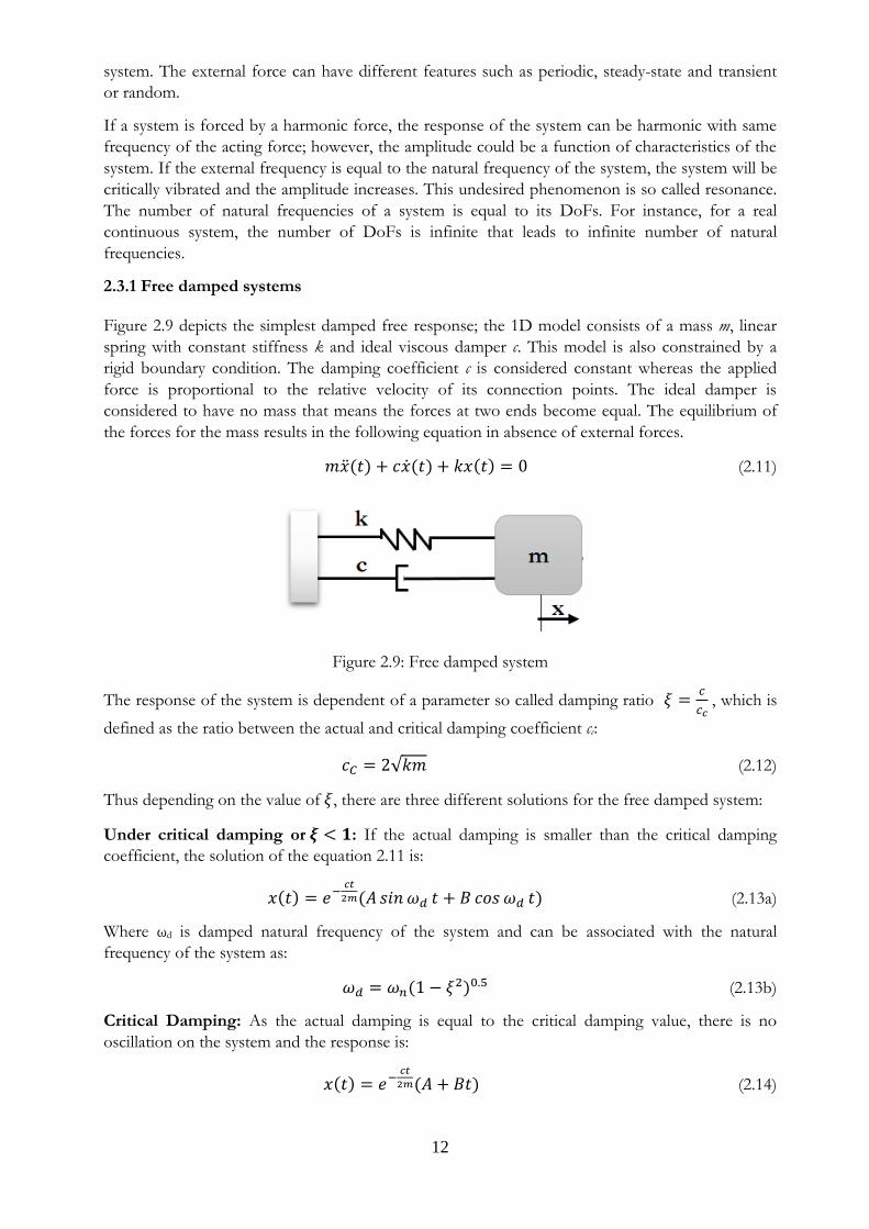
2.3.1 Free damped systems Figure 2.9 depicts the simplest damped free response; the 1D model consists of a mass m, linear

spring with constant stiffness k and ideal viscous damper c. This model is also constrained by a

rigid boundary condition. The damping coefficient c is considered constant whereas the applied

force is proportional to the relative velocity of its connection points. The ideal damper is

considered to have no mass that means the forces at two ends become equal. The equilibrium of

the forces for the mass results in the following equation in absence of external forces.

𝑚�̈�(𝑡) + 𝑐�̇�(𝑡) + 𝑘𝑥(𝑡) = 0 (2.11)

Figure 2.9: Free damped system

The response of the system is dependent of a parameter so called damping ratio 𝜉 =𝑐

𝑐𝑐 , which is

defined as the ratio between the actual and critical damping coefficient cc:

𝑐𝐶 = 2√𝑘𝑚 (2.12)

Thus depending on the value of 𝜉, there are three different solutions for the free damped system:

Under critical damping or 𝝃 < 𝟏: If the actual damping is smaller than the critical damping

coefficient, the solution of the equation 2.11 is:

𝑥(𝑡) = 𝑒−𝑐𝑡

2𝑚(𝐴 𝑠𝑖𝑛 𝜔𝑑 𝑡 + 𝐵 𝑐𝑜𝑠 𝜔𝑑 𝑡) (2.13a)

Where ωd is damped natural frequency of the system and can be associated with the natural

frequency of the system as:

𝜔𝑑 = 𝜔𝑛(1 − 𝜉2)0.5 (2.13b)

Critical Damping: As the actual damping is equal to the critical damping value, there is no

oscillation on the system and the response is:

𝑥(𝑡) = 𝑒−𝑐𝑡

2𝑚(𝐴 + 𝐵𝑡) (2.14)

13

Over critical damping or 𝝃 > 𝟏: It occurs when actual damping value is higher than the critical

damping coefficient, then the response of the system is:

𝑥(𝑡) = (𝐴𝑒𝑟1𝑡 + 𝐵𝑒𝑟2𝑡) (2.15)

Where r1 and r2 are defined as:

𝑟1,2 =−𝑐±√𝑐2−4𝑚𝑘

2𝑚 (2.16)

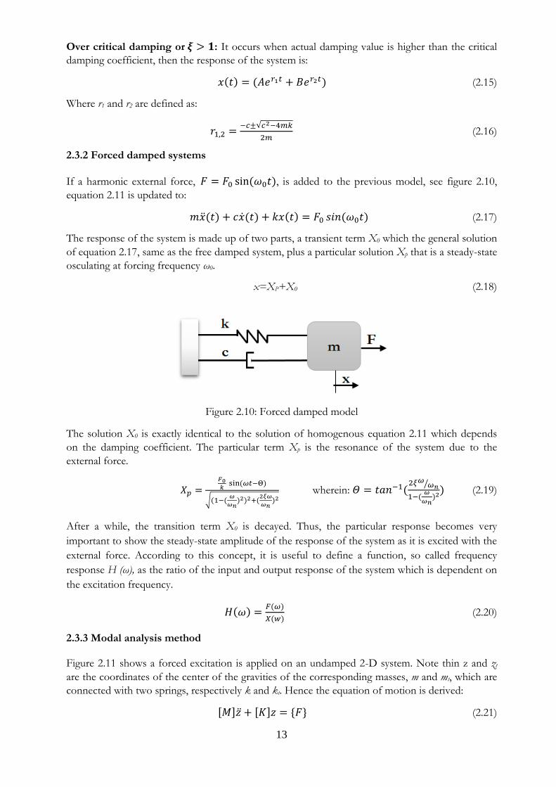
2.3.2 Forced damped systems

If a harmonic external force, 𝐹 = 𝐹0 sin(𝜔0𝑡), is added to the previous model, see figure 2.10,

equation 2.11 is updated to:

𝑚�̈�(𝑡) + 𝑐�̇�(𝑡) + 𝑘𝑥(𝑡) = 𝐹0 𝑠𝑖𝑛(𝜔0𝑡) (2.17)

The response of the system is made up of two parts, a transient term X0 which the general solution

of equation 2.17, same as the free damped system, plus a particular solution Xp that is a steady-state

osculating at forcing frequency ω0.

x=XP+X0 (2.18)

Figure 2.10: Forced damped model

The solution X0 is exactly identical to the solution of homogenous equation 2.11 which depends

on the damping coefficient. The particular term Xp is the resonance of the system due to the

external force.

𝑋𝑝 =𝐹0𝑘

sin(𝜔𝑡−Θ)

√(1−(𝜔

𝜔𝑛)2)2+(

2𝜉𝜔

𝜔𝑛)2

wherein: 𝛩 = 𝑡𝑎𝑛−1(2𝜉𝜔

𝜔𝑛⁄

1−(𝜔

𝜔𝑛)2

) (2.19)

After a while, the transition term X0 is decayed. Thus, the particular response becomes very

important to show the steady-state amplitude of the response of the system as it is excited with the

external force. According to this concept, it is useful to define a function, so called frequency

response H (ω), as the ratio of the input and output response of the system which is dependent on

the excitation frequency.

𝐻(𝜔) =𝐹(𝜔)

𝑋(𝑤) (2.20)

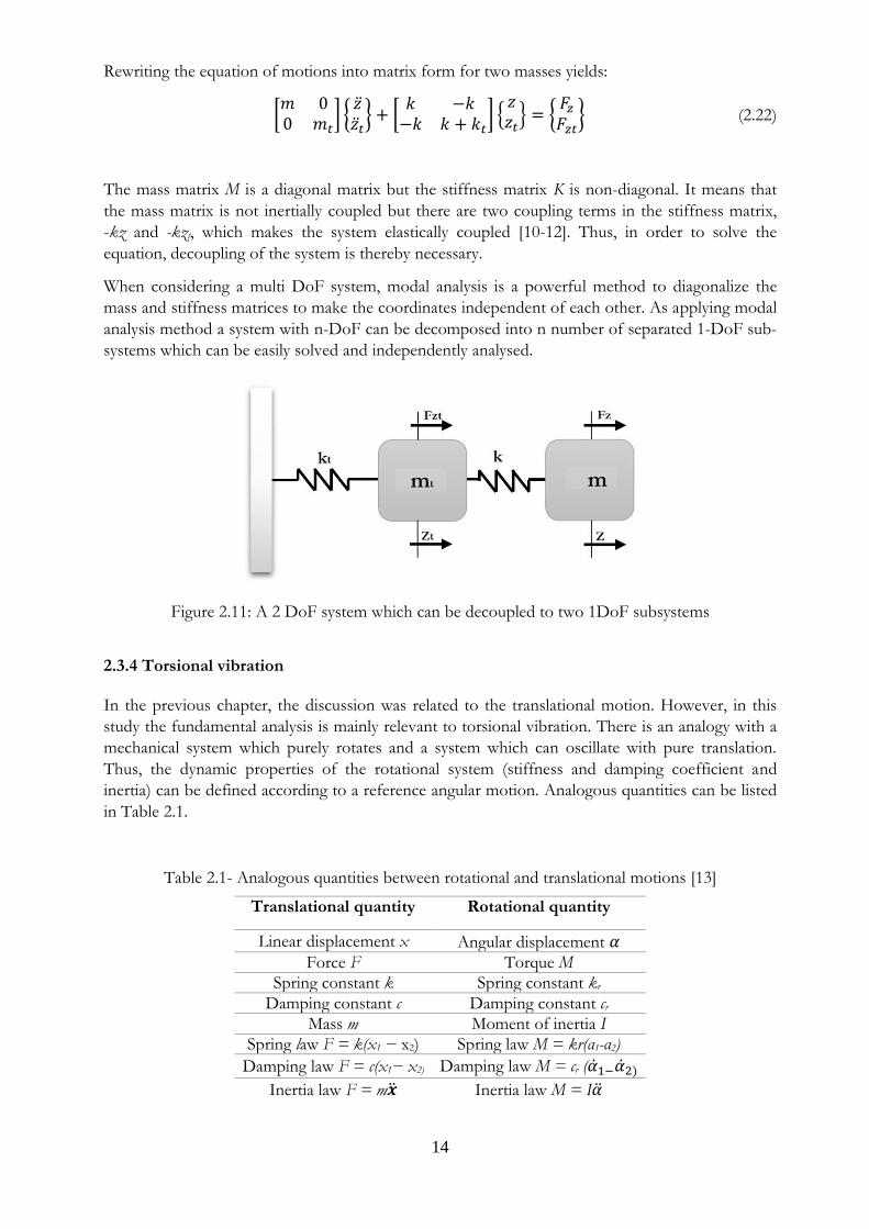
2.3.3 Modal analysis method Figure 2.11 shows a forced excitation is applied on an undamped 2-D system. Note thin z and zt

are the coordinates of the center of the gravities of the corresponding masses, m and mt, which are

connected with two springs, respectively k and kt. Hence the equation of motion is derived:

[𝑀]�̈� + [𝐾]𝑧 = {𝐹} (2.21)

14

Rewriting the equation of motions into matrix form for two masses yields:

[𝑚 00 𝑚𝑡

] {�̈��̈�𝑡

} + [𝑘 −𝑘

−𝑘 𝑘 + 𝑘𝑡] {

𝑧𝑧𝑡

} = {𝐹𝑧

𝐹𝑧𝑡} (2.22)

The mass matrix M is a diagonal matrix but the stiffness matrix K is non-diagonal. It means that

the mass matrix is not inertially coupled but there are two coupling terms in the stiffness matrix,

-kz and -kzt, which makes the system elastically coupled [10-12]. Thus, in order to solve the

equation, decoupling of the system is thereby necessary.

When considering a multi DoF system, modal analysis is a powerful method to diagonalize the

mass and stiffness matrices to make the coordinates independent of each other. As applying modal

analysis method a system with n-DoF can be decomposed into n number of separated 1-DoF sub-

systems which can be easily solved and independently analysed.

Figure 2.11: A 2 DoF system which can be decoupled to two 1DoF subsystems

2.3.4 Torsional vibration In the previous chapter, the discussion was related to the translational motion. However, in this

study the fundamental analysis is mainly relevant to torsional vibration. There is an analogy with a

mechanical system which purely rotates and a system which can oscillate with pure translation.

Thus, the dynamic properties of the rotational system (stiffness and damping coefficient and

inertia) can be defined according to a reference angular motion. Analogous quantities can be listed

in Table 2.1.

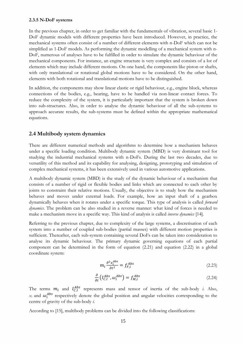
Table 2.1- Analogous quantities between rotational and translational motions [13]

Translational quantity Rotational quantity

Linear displacement x Angular displacement 𝛼

Force F Torque M

Spring constant k Spring constant kr

Damping constant c Damping constant cr

Mass m Moment of inertia I

Spring law F = k(x1 − x2) Spring law M = kr(α1-α2)

Damping law F = c(x1− x2) Damping law M = cr (�̇�1−�̇�2)

Inertia law F = m�̈� Inertia law M = I�̈�

15

2.3.5 N-DoF systems In the previous chapter, in order to get familiar with the fundamentals of vibration, several basic 1-

DoF dynamic models with different properties have been introduced. However, in practice, the

mechanical systems often consist of a number of different elements with n-DoF which can not be

simplified as 1-DoF models. As performing the dynamic modelling of a mechanical system with n-

DoF, numerous of analyses have to be fulfilled in order to simulate the dynamic behaviour of the

mechanical components. For instance, an engine structure is very complex and consists of a lot of

elements which may include different motions. On one hand, the components like piston or shafts,

with only translational or rotational global motions have to be considered. On the other hand,

elements with both rotational and translational motions have to be distinguished.

In addition, the components may show linear elastic or rigid behaviour, e.g., engine block, whereas

connections of the bodies, e.g., bearing, have to be handled via non-linear contact forces. To

reduce the complexity of the system, it is particularly important that the system is broken down

into sub-structures. Also, in order to analyse the dynamic behaviour of all the sub-systems to

approach accurate results, the sub-systems must be defined within the appropriate mathematical

equations.

2.4 Multibody system dynamics There are different numerical methods and algorithms to determine how a mechanism behaves

under a specific loading condition. Multibody dynamic system (MBD) is very dominant tool for

studying the industrial mechanical systems with n-DoFs. During the last two decades, due to

versatility of this method and its capability for analysing, designing, prototyping and simulation of

complex mechanical systems, it has been extensively used in various automotive applications.

A multibody dynamic system (MBD) is the study of the dynamic behaviour of a mechanism that

consists of a number of rigid or flexible bodies and links which are connected to each other by

joints to constraint their relative motions. Usually, the objective is to study how the mechanism

behaves and moves under external loads. For example, how an input shaft of a gearbox

dynamically behaves when it rotates under a specific torque. This type of analysis is called forward

dynamics. The problem can be also studied in a reverse manner: what kind of forces is needed to

make a mechanism move in a specific way. This kind of analysis is called inverse dynamics [14].

Referring to the previous chapter, due to complexity of the large systems, a discretisation of each

system into a number of coupled sub-bodies (partial masses) with different motion properties is

sufficient. Thereafter, each sub-system containing several DoFs can be taken into consideration to

analyse its dynamic behaviour. The primary dynamic governing equations of each partial

component can be determined in the form of equation (2.21) and equation (2.22) in a global

coordinate system:

𝑚𝑖𝜕2𝑥𝑖

𝐴𝑏𝑠

𝜕𝑡2= 𝑓𝐹,𝑖

𝐴𝑏𝑠 (2.23)

𝜕

𝜕𝑡(𝐼𝐶.𝐼

𝐴𝑏𝑠, 𝜔𝑖𝐴𝑏𝑠) = 𝑓𝑀,𝑖

𝐴𝑏𝑠 (2.24)

The terms 𝑚𝑖 and 𝐼𝐶.𝐼𝐴𝑏𝑠 represents mass and tensor of inertia of the sub-body i. Also,

xi and 𝜔𝑖𝐴𝑏𝑠 respectively denote the global position and angular velocities corresponding to the

centre of gravity of the sub-body i.

According to [15], multibody problems can be divided into the following classifications:

16

• Rigid body problems

• Linearly elastic or flexible problems

• Non-linearly elastic multibody systems

Deriving the equations of multibody dynamics of each category is beyond the scope of this thesis.

A lot of details can be found in [16]. It is recommended to the reader to consider the reference to

realize how each category is taken into account.

2.4.1 AVL Excite power unit Over the last decades, multibody dynamic commercial simulation tools have been rapidly

developed to be used in automotive applications. These methods have some advantageous in

comparison with experimental techniques: It allows that the engineers can easily observe how a

mechanism performs and shorten the product design cycle without building it that saves a lot of

money and time [14].

For this study, AVL Excite Power Unit module is chosen to simulate the powertrain and study

NVH analysis. This software is a specialized tool for simulation of flexible and rigid bodies of

powertrains by proposing a broad range of versatile applications:

• Multi-level approach – modelling depth adjustable to application target

• Proposing prominent lubricated contact models

• Modelling of specific transmission/driveline components

• Diversity of electric machine models [17]

2.4.2 AVL Excite power unit component modelling AVL Excite provides a wide range of joint models such as spring damper models, gear contact and

bearings, with linear or non-linear behaviour. Also, it prepares different possibilities for modelling

of rigid and flexible mechanical components like shaft or joints. The models are available in AVL

Excite’s library and can be used for different applications like internal combustion engines or

electrify transmission line. In this section, due to important roles of gear and bearing contacts, it

will be discussed how they are modelled in AVL excite. The mathematical formulation of each

joint model is extensively explained in [16] and it is recommended to the reader to refer to the

reference to get more details.

2.4.2.1 Advanced Cylindrical Gear Joint (ACYG) AVL/Excite provides two choices for modelling of gears, Generic Gear Joints and Advanced Cylindrical

Gear Joint. In contrast to Generic Gear Joints, Advanced Cylindrical Gear Joint (ACYG) is an acceptable

feature for dynamic modelling of cylindrical gears (spur and helical) with parallel axis only and

provides more details where flank surfaces play a major influence [16]. For instance:

• Gear whine

• Dynamic transmission error (DTE)

• Edge loading (angular gear misalignments)

• Gear corrections/modifications

• Power loss

• Meshing forces as a basis for flank contact pressure and root stress calculations

• Computation of effective meshing stiffness [16]

17

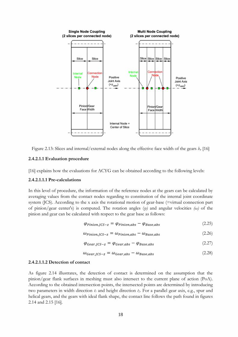
In the Advanced Cylindrical Gear Joint (ACYG) model, the bodies (gear and pinion) are coupled to

each other via nodes located on the bodies’ axis of rotation. In addition, a discretization into slices

along the width of gears is necessary to approach acceptable resolution in the gear flank area

whereas the slices behave as uncoupled from their adjacent slices [16].

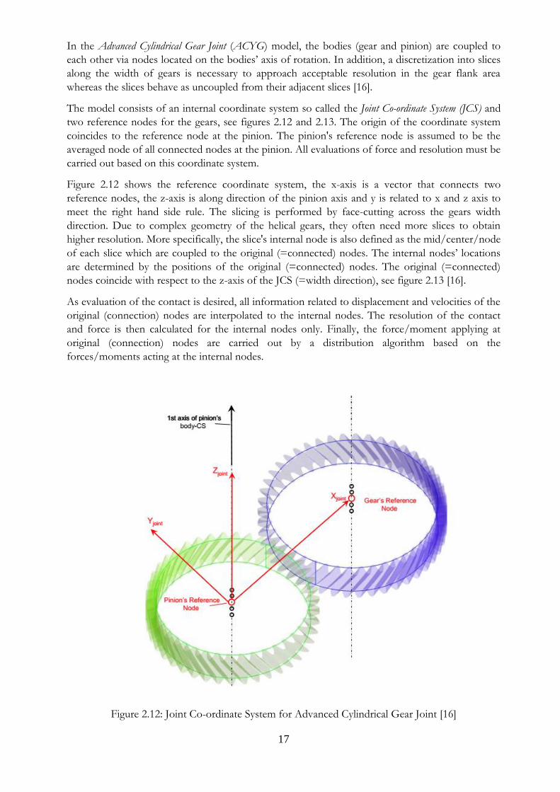
The model consists of an internal coordinate system so called the Joint Co-ordinate System (JCS) and

two reference nodes for the gears, see figures 2.12 and 2.13. The origin of the coordinate system

coincides to the reference node at the pinion. The pinion's reference node is assumed to be the

averaged node of all connected nodes at the pinion. All evaluations of force and resolution must be

carried out based on this coordinate system.

Figure 2.12 shows the reference coordinate system, the x-axis is a vector that connects two

reference nodes, the z-axis is along direction of the pinion axis and y is related to x and z axis to

meet the right hand side rule. The slicing is performed by face-cutting across the gears width

direction. Due to complex geometry of the helical gears, they often need more slices to obtain

higher resolution. More specifically, the slice's internal node is also defined as the mid/center/node

of each slice which are coupled to the original (=connected) nodes. The internal nodes’ locations

are determined by the positions of the original (=connected) nodes. The original (=connected)

nodes coincide with respect to the z-axis of the JCS (=width direction), see figure 2.13 [16].

As evaluation of the contact is desired, all information related to displacement and velocities of the

original (connection) nodes are interpolated to the internal nodes. The resolution of the contact

and force is then calculated for the internal nodes only. Finally, the force/moment applying at

original (connection) nodes are carried out by a distribution algorithm based on the

forces/moments acting at the internal nodes.

Figure 2.12: Joint Co-ordinate System for Advanced Cylindrical Gear Joint [16]

18

Figure 2.13: Slices and internal/external nodes along the effective face width of the gears bw [16]

2.4.2.1.1 Evaluation procedure

[16] explains how the evaluations for ACYG can be obtained according to the following levels:

2.4.2.1.1.1 Pre-calculations In this level of procedure, the information of the reference nodes at the gears can be calculated by

averaging values from the contact nodes regarding to constitution of the internal joint coordinate

system (JCS). According to the x axis the rotational motion of gear-base (=virtual connection part

of pinion/gear center's) is computed. The rotation angles (φ) and angular velocities (ω) of the

pinion and gear can be calculated with respect to the gear base as follows:

𝜑𝑃𝑖𝑛𝑖𝑜𝑛,𝐽𝐶𝑆−𝑧 = 𝜑𝑃𝑖𝑛𝑖𝑜𝑛,𝑎𝑏𝑠 − 𝜑𝐵𝑎𝑠𝑒,𝑎𝑏𝑠 (2.25)

𝜔𝑃𝑖𝑛𝑖𝑜𝑛,𝐽𝐶𝑆−𝑧 = 𝜔𝑃𝑖𝑛𝑖𝑜𝑛,𝑎𝑏𝑠 − 𝜔𝐵𝑎𝑠𝑒,𝑎𝑏𝑠 (2.26)

𝜑𝐺𝑒𝑎𝑟,𝐽𝐶𝑆−𝑧 = 𝜑𝐺𝑒𝑎𝑟,𝑎𝑏𝑠 − 𝜑𝐵𝑎𝑠𝑒,𝑎𝑏𝑠 (2.27)

𝜔𝐺𝑒𝑎𝑟,𝐽𝐶𝑆−𝑧 = 𝜔𝐺𝑒𝑎𝑟,𝑎𝑏𝑠 − 𝜔𝐵𝑎𝑠𝑒,𝑎𝑏𝑠 (2.28)

2.4.2.1.1.2 Detection of contact As figure 2.14 illustrates, the detection of contact is determined on the assumption that the

pinion/gear flank surfaces in meshing must also intersect to the current plane of action (PoA).

According to the obtained intersection points, the intersected points are determined by introducing

two parameters in width direction t1 and height direction t2. For a parallel gear axis, e.g., spur and

helical gears, and the gears with ideal flank shape, the contact line follows the path found in figures

2.14 and 2.15 [16].

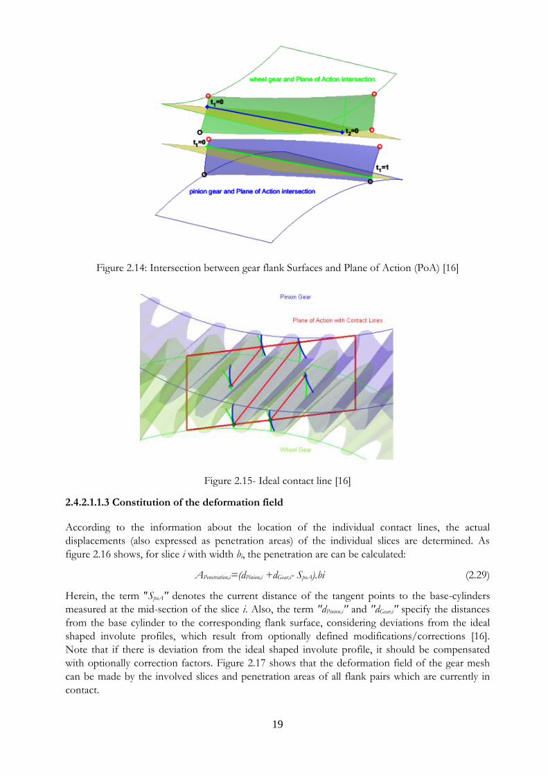
19

Figure 2.14: Intersection between gear flank Surfaces and Plane of Action (PoA) [16]

Figure 2.15- Ideal contact line [16]

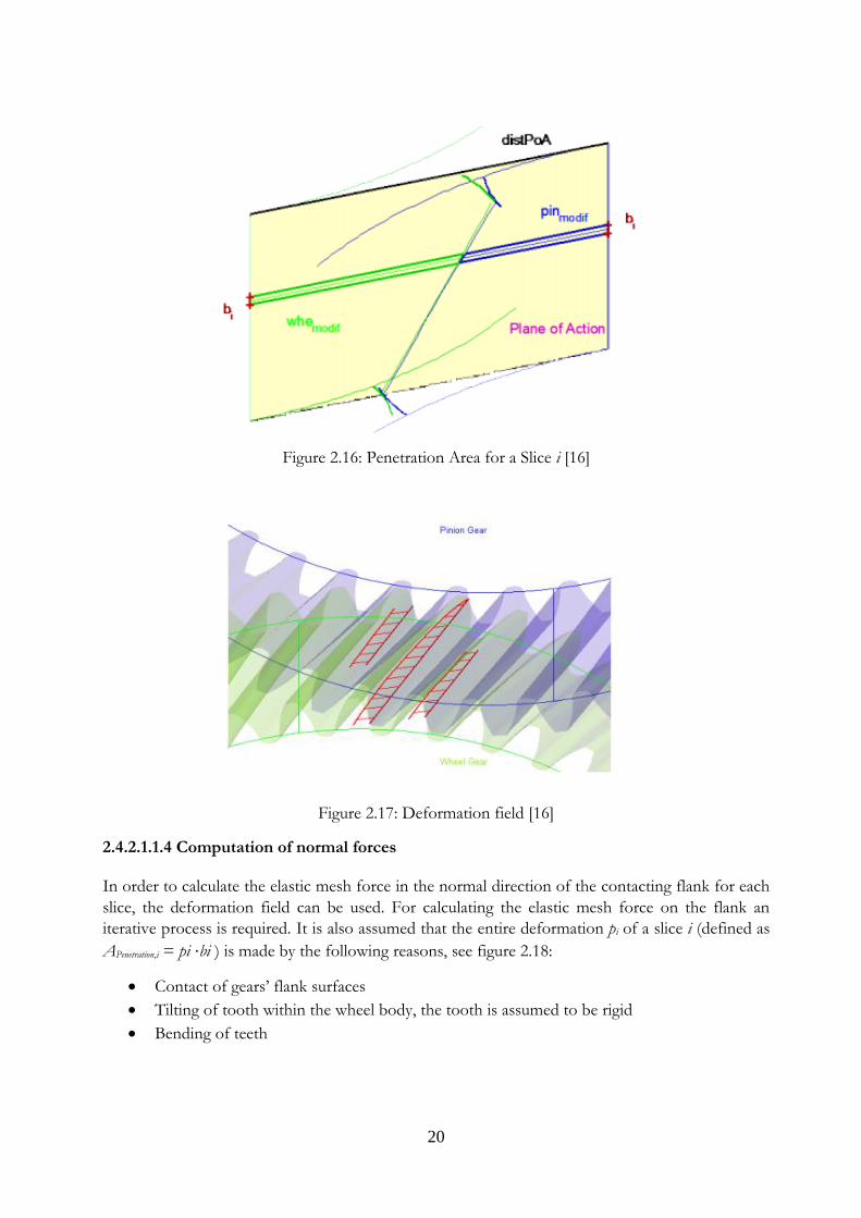
2.4.2.1.1.3 Constitution of the deformation field According to the information about the location of the individual contact lines, the actual

displacements (also expressed as penetration areas) of the individual slices are determined. As

figure 2.16 shows, for slice i with width bi, the penetration are can be calculated:

APenetration,i=(dPinion,i +dGear,i- SpoA).bi (2.29)

Herein, the term "SpoA" denotes the current distance of the tangent points to the base-cylinders

measured at the mid-section of the slice i. Also, the term "dPinion,i" and "dGear,i" specify the distances

from the base cylinder to the corresponding flank surface, considering deviations from the ideal

shaped involute profiles, which result from optionally defined modifications/corrections [16].

Note that if there is deviation from the ideal shaped involute profile, it should be compensated

with optionally correction factors. Figure 2.17 shows that the deformation field of the gear mesh

can be made by the involved slices and penetration areas of all flank pairs which are currently in

contact.

20

Figure 2.16: Penetration Area for a Slice i [16]

Figure 2.17: Deformation field [16]

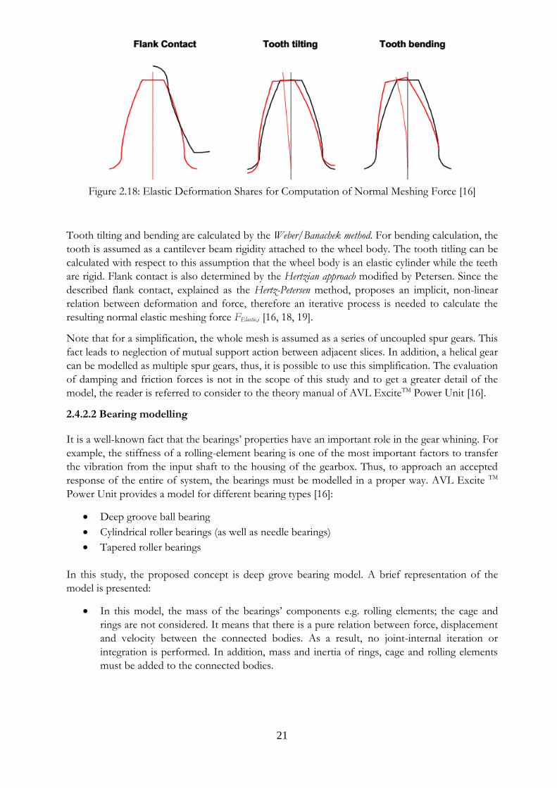
2.4.2.1.1.4 Computation of normal forces In order to calculate the elastic mesh force in the normal direction of the contacting flank for each

slice, the deformation field can be used. For calculating the elastic mesh force on the flank an

iterative process is required. It is also assumed that the entire deformation pi of a slice i (defined as

APenetration,i = pi ⋅bi ) is made by the following reasons, see figure 2.18:

• Contact of gears’ flank surfaces

• Tilting of tooth within the wheel body, the tooth is assumed to be rigid

• Bending of teeth

21

Figure 2.18: Elastic Deformation Shares for Computation of Normal Meshing Force [16]

Tooth tilting and bending are calculated by the Weber/Banachek method. For bending calculation, the

tooth is assumed as a cantilever beam rigidity attached to the wheel body. The tooth titling can be

calculated with respect to this assumption that the wheel body is an elastic cylinder while the teeth

are rigid. Flank contact is also determined by the Hertzian approach modified by Petersen. Since the

described flank contact, explained as the Hertz-Petersen method, proposes an implicit, non-linear

relation between deformation and force, therefore an iterative process is needed to calculate the

resulting normal elastic meshing force FElastic,i [16, 18, 19].

Note that for a simplification, the whole mesh is assumed as a series of uncoupled spur gears. This

fact leads to neglection of mutual support action between adjacent slices. In addition, a helical gear

can be modelled as multiple spur gears, thus, it is possible to use this simplification. The evaluation

of damping and friction forces is not in the scope of this study and to get a greater detail of the

model, the reader is referred to consider to the theory manual of AVL ExciteTM Power Unit [16].

2.4.2.2 Bearing modelling It is a well-known fact that the bearings’ properties have an important role in the gear whining. For

example, the stiffness of a rolling-element bearing is one of the most important factors to transfer

the vibration from the input shaft to the housing of the gearbox. Thus, to approach an accepted

response of the entire of system, the bearings must be modelled in a proper way. AVL Excite TM

Power Unit provides a model for different bearing types [16]:

• Deep groove ball bearing

• Cylindrical roller bearings (as well as needle bearings)

• Tapered roller bearings

In this study, the proposed concept is deep grove bearing model. A brief representation of the

model is presented:

• In this model, the mass of the bearings’ components e.g. rolling elements; the cage and

rings are not considered. It means that there is a pure relation between force, displacement

and velocity between the connected bodies. As a result, no joint-internal iteration or

integration is performed. In addition, mass and inertia of rings, cage and rolling elements

must be added to the connected bodies.

22

• The model relies on a center to center coupling and raceways of the bearings always hold

pure circular. Consequently, shaft and housing borne elastic deformation do not influence

on the geometry of outer/inner ring raceways.

• Hertz’s formula for spherically shaped surfaces is applied to make the contact between

rolling elements and inner/outer ring’s raceways. Also, an empirical approach according to

Kunert is used for cylindrical roller bearings. In this model, hydrodynamic contribution in

the zone of contact is not considered at all.

• Motion of rolling elements is analysed as a purely kinematic behaviour by assuming perfect

rolling. As a result, slip between rolling elements and inner/outer ring raceways can be

ignored.

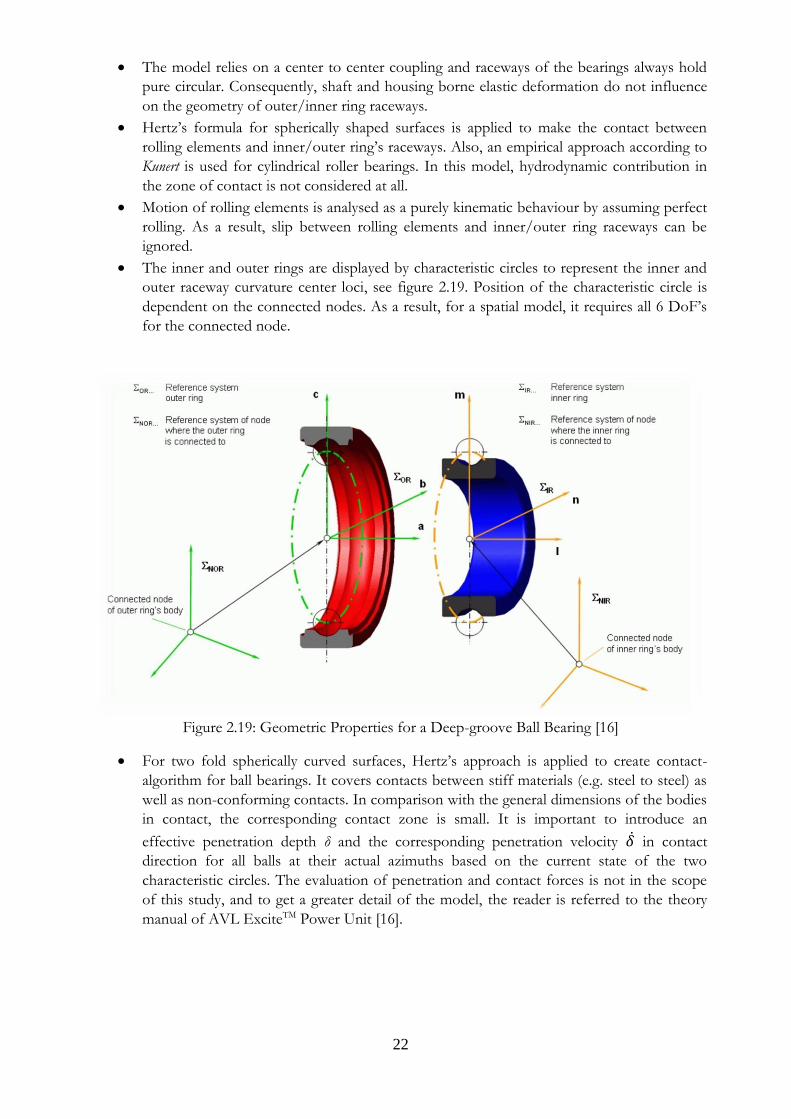
• The inner and outer rings are displayed by characteristic circles to represent the inner and

outer raceway curvature center loci, see figure 2.19. Position of the characteristic circle is

dependent on the connected nodes. As a result, for a spatial model, it requires all 6 DoF’s

for the connected node.

Figure 2.19: Geometric Properties for a Deep-groove Ball Bearing [16]

• For two fold spherically curved surfaces, Hertz’s approach is applied to create contact-

algorithm for ball bearings. It covers contacts between stiff materials (e.g. steel to steel) as

well as non-conforming contacts. In comparison with the general dimensions of the bodies

in contact, the corresponding contact zone is small. It is important to introduce an

effective penetration depth δ and the corresponding penetration velocity �̇� in contact

direction for all balls at their actual azimuths based on the current state of the two

characteristic circles. The evaluation of penetration and contact forces is not in the scope

of this study, and to get a greater detail of the model, the reader is referred to the theory

manual of AVL ExciteTM Power Unit [16].

23

2.5 Sub-structuring concept Significant advances in different fields of engineering, such as fluid mechanics, aerospace and

automotive engineering, have been led to mathematical problems with partial differential equations

(PDE). Often, in order to solve the PDE problems, it is impossible to obtain analytical

approaches. Hence, there are a number of numerical methods that have been introduced to solve

these types of problems.

Today, finite element solutions (FEM) are very useful tools in science and technology applications

and there are a various types of the FEM commercial codes. FEM methods were introduced in

1950’s and, gradually with developing the computer science and technology in 1970’s, have been

very popular in all engineering fields. In the beginning of releasing the computers, due to lack of

technology, it was very time consuming to solve a large engineering problem by using numerical

methods. In general, when it comes to numerical methods, it is very important to reduce the

runtime. Although the speed of computers has been multiplied through the last decades, the

powerful computers are still very expensive. Hence, besides of the advanced computer technology,

it has been very important to simplify a complex problem to save time and money.

In this point of view, especially in computational dynamics, the combinations of a large complex

domain with detailed model and discretizing in small time step often cause to increase the

simulation runtime simulation. In order to overcome to this limitation, it is essential to simplify the

dynamic problems. One idea is to use structural elements, such as beams and shells, to simulate the

behaviour of the entire original problem. However, this method is not appropriate for a problem

with complex geometry and boundary conditions. Another solution is to use reduction methods to

reduce the DoFs. In this mathematical method, the DoFs are divided into two categories, master,

which are still available after operation, and slave DoFs.

One reduction method is the Guyan-Irons reduction method which is very suitable especially for

static problems. This method also shows acceptable results for dynamic problems with low

frequency or if the load is not applied suddenly. Nevertheless, this method is not proper for

dynamic problems with high-frequency range because an appropriate reduction of the mass matrix

must be implemented. Another reduction concept is the Craig-Bampton method which is quite

suitable for dynamic problems in high frequency range. In this method the structure is divided into

small dynamic substructures which can be reduced independently. Afterwards, the substructures

can be assembled to the original condition [20, 21].

This idea has been introduced in the early 1960’s by aerospace engineers when the computers had

not large memory to solve the complex aerospace problems. The aim was to simplify the complex

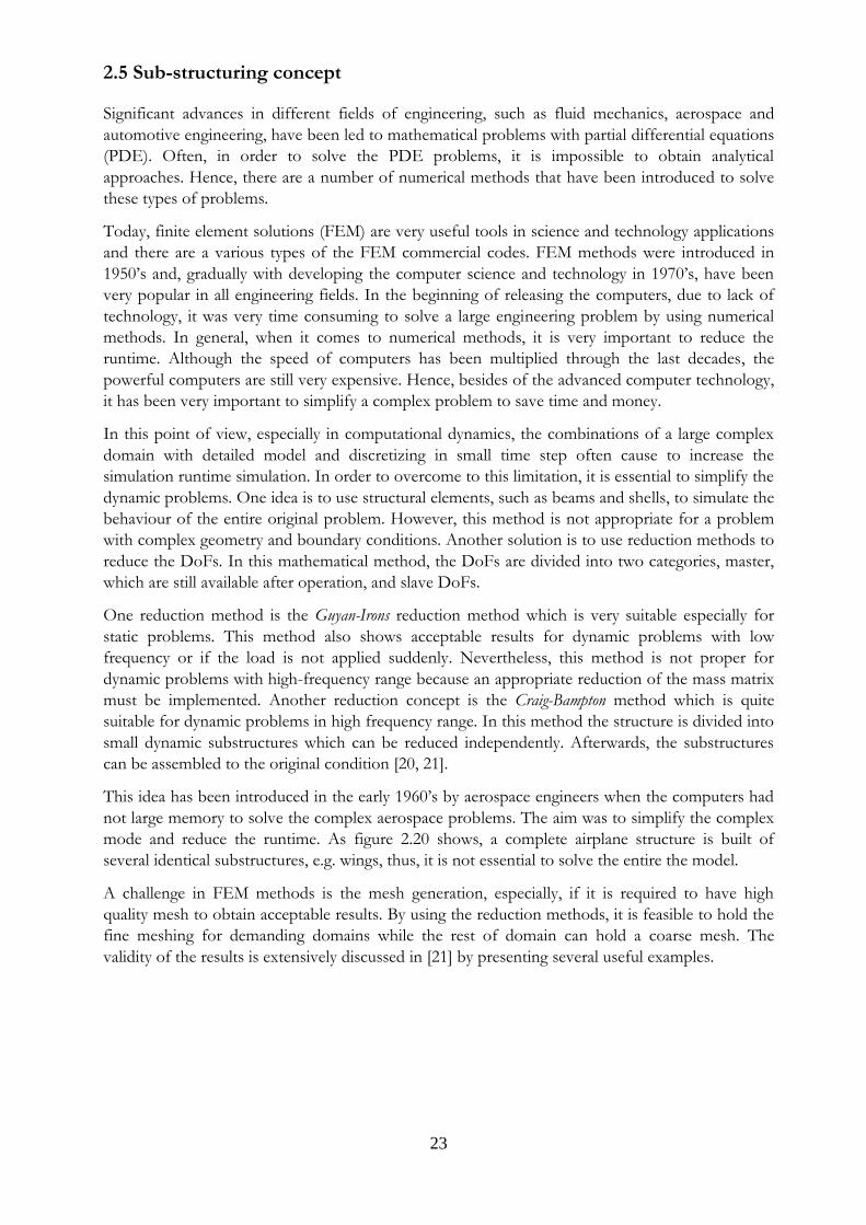
mode and reduce the runtime. As figure 2.20 shows, a complete airplane structure is built of

several identical substructures, e.g. wings, thus, it is not essential to solve the entire the model.

A challenge in FEM methods is the mesh generation, especially, if it is required to have high

quality mesh to obtain acceptable results. By using the reduction methods, it is feasible to hold the

fine meshing for demanding domains while the rest of domain can hold a coarse mesh. The

validity of the results is extensively discussed in [21] by presenting several useful examples.

24

Figure 2.20: The entire structure can be broken into a number of substructure levels, S1 to S6 [22]

The dynamic substructuring has several advantageous as below:

• It reduces the total number of DoFs from millions to thousands. Thus, it is possible to

study a very detailed model and reduce the runtime. Furthermore, a reduced system needs

less computational resource and it is easier to be implemented and save money.

• It simplifies the model and allows reducing the entire structure so that it gets rid of those

subdomains that do not contributes to the dynamic behaviour of the model.

2.5.1 Craig-Bampton method In this method, the degrees of freedom (DoF) are partitioned into two different types, a boundary

part or b as a master and an interior part or i as slave DoFs. Hence, the semi-discrete equation of

motion, equations 2.30 and 2.31, can be formed as:

𝑀�̈�(𝑡) + 𝐾𝑢(𝑡) = 𝐹(𝑡) (2.30)

[𝑀𝑖𝑖 𝑀𝑖𝑏

𝑀𝑏𝑖 𝑀𝑏𝑏] [

�̈�𝑖

�̈�𝑏] + [

𝐾𝑖𝑖 𝐾𝑖𝑏

𝐾𝑏𝑖 𝐾𝑏𝑏] [

𝑢𝑖

𝑢𝑏] = [

𝐹𝑖

𝐹𝑏] (2.31)

In principle, this method reduces the internal degrees of freedom by defining a number of internal

modes. This reduction method needs two different types of modes, the fixed-interface vibration

modes (normal modes) and the constraint modes.

2.5.1.1 The fixed-interface vibration modes In order to calculate the normal modes, it is required to refer to the eigenvalue problem containing

the internal mass and stiffness matrices. More specifically, as discussed earlier, the whole system

must be partitioned into internal and boundary degrees of freedom. These modes represents the

information associated with the vibrations of the system and must be held fixed at its boundary

DOF, i.e. ({𝑥𝑏} = 0), that leads to reduce equation 2.31 as:

[𝑀𝑖𝑖][�̈�𝑖] + [𝐾𝑖𝑖][𝑢𝑖] = 0 (2.32)

And finally, in order to solve this eigenvalue problem, containing n eigenvalues (λ) and

eigenvectors (Φ), the following equation can be solved

(Kii − λj2 Mii ) {Φi}j = 0 where j = 1,2, … … … n. (2.33)

In NVH problems, high frequencies have often little effect on the characteristics of the system.

Therefore, they can be ignored. The results are the eigen-frequencies and eigen-modes of the

25

system and the remaining k fixed-interface vibration modes which are represent in the modal

format.

[Φ𝑖𝑘

0] = [

{𝛷𝑖𝑘}1 {𝛷𝑖𝑘}2 … {𝛷𝑖𝑘}𝑘

0 0 … 0] (2.34)

2.5.1.2 Constraint modes The other sort of mode used in Craig-Bampton is constraint mode. This mode results from the static

deformation of the system due to applying a unit displacement to one of the boundary DoF.

Simultaneously, the other interface DoF must be held restrained and there is no force acting on the

internal degrees of freedom.

In principle, the constraint modes are the static response of the structure because of a unit

deformation applied on the interface DoF. In order to calculate these modes, which is identical to

calculate the normal modes, the total DoF of the system must be also divided into the internal and

boundary DoF. Thus, with the assumption of the free-force internal DoF, the equation 2.31 can be

summarized as:

[𝑀𝑖𝑖][�̈�𝑖] + [𝑀𝑖𝑏][�̈�𝑏] + [𝐾𝑖𝑖][𝑢𝑖] + [𝐾𝑖𝑏][𝑢𝑏] = 0 (2.35)

Furthermore, in order to calculate the static response, the inertia terms can be neglected. This

assumption reduces the equation 2.32 as:

{𝑢𝑖 (𝑆𝑡𝑎𝑡𝑖𝑐)} = −[𝐾𝑖𝑖]−1[𝐾𝑖𝑏][𝑢𝑏] (2.36)

The term −[𝐾𝑖𝑖]−1[𝐾𝑖𝑏] is known as static mode matrix. Now, having the static mode matrix leads to

write the constraint modes matrix:

[{𝑥𝑖}

{𝑥𝑏}] = [𝛷𝐶]{𝑥𝑏} = [

−[𝐾𝑖𝑖]−1[𝐾𝑖𝑏]

[𝐼]] {𝑥𝑏} (2.37)

where [Φ𝐶] is the constraint modes matrix.

2.5.1.3 Reduction matrix As previously discussed, the aim of applying the Craig-Bampton method is to reduce the structure

and total DoFs to decrease the runtime. After calculating the normal and constrained modes, it is

possible to obtain the reduction matrix. The reduction matric [R]CB is necessary to reduce the

structure. In order to calculate the reduction matrix, the internal DoF must be described in

combinations of the normal modes [𝛷𝑖] and constraint modes [𝛷𝐶].

{𝑥𝑖} = [𝛷𝑖]{𝜂𝑖} + [𝛷𝐶]{𝑥𝑏} (2.38)

Replacing into original DoF leads that the reduction becomes in the following form:

[{𝑥𝑖}

{𝑥𝑏}] = [

[𝛷𝑖]{𝜂𝑖} + [𝛷𝐶]{𝑥𝑏}

{𝑥𝑏}] = [

[𝛷𝑖] [𝛷𝐶]0 [𝐼]

] [{𝜂𝑖}

{𝑥𝑏}] = [𝑅]𝐶𝐵 [

{𝜂𝑖}

{𝑥𝑏}] (2.39)

Once the reduction matrix is available, in order to reduce the original structure, it is possible to

reduce the original mass and stiffness matrices:

{[�̃�]𝐶𝐵 = [𝑅]𝐶𝐵

𝑇 [𝑀][𝑅]𝐶𝐵

[�̃�]𝐶𝐵 = [𝑅]𝐶𝐵𝑇 [𝐾][𝑅]𝐶𝐵

(2.40)

26

Reduced matrices have dramatically smaller dimensions. [21] presents several useful examples

when the reduction method is applied on the original matrix structure and significantly reduced the

size of the matrices.

2.6 Rayleigh damping The internal damping of the components is defined according to Rayleigh damping method. This

method is broadly applied to analyse internal structural damping. Rayleigh damping is a viscous

damping that is a linear combination of mass and stiffness:

C=α1M+α2K (2.41a)

where M and K are the mass and stiffness matrices and α1 and α2 are constants of proportionality.

The constants can be calculated according to the frequencies (f) and damping ratios (𝜁):

𝜁 = 𝜋(𝛼1

𝑓+ 𝛼2𝑓) (2.41b)

Hence, in order to calculate the constants, the frequencies and damping ratios must be predefined.

2.7 Fast Fourier Transform (FFT) In mathematics, according to the Fourier series, a periodic signal as a function of time, with time

period T, can be decomposed into an infinite numbers of harmonic signals, namely sines and

cosines terms (or similarly, complex exponential). The frequency of each term is the frequency of

the original signal and its multiplication which is so called harmonic of the signal. Consequently,

equation 2.42 shows the decomposition of the original function f (t) into a series of harmonics

where ω0 =2π/T [23].

𝑓(𝑡) = 𝑎0 + ∑ (𝑎𝑛 𝑐𝑜𝑠 𝜔0𝑛𝑡 + 𝑏𝑛 𝑠𝑖𝑛 𝜔0𝑛𝑡)∞𝑛=1 (2.42)

where the constants a0, an and bn are defined as:

𝑎0 =1

𝑇∫ 𝑓(𝑡)𝑑𝑡

𝑇

0 (2.43)

𝑎𝑛 =2

𝑇∫ 𝑓(𝑡) cos 𝜔0𝑛𝑡𝑑𝑡

𝑇

0 (2.44)

𝑏𝑛 =2

𝑇∫ 𝑓(𝑡) sin 𝜔0𝑛𝑡𝑑𝑡

𝑇

0 (2.45)

Alternatively an infinite series can be expressed into complex exponential terms:

𝑓(𝑡) = ∑ 𝑐𝑛+∞𝑛=−∞ 𝑒𝑗𝜔𝑛𝑡 (2.46)

Herein 𝑐𝑛 =1

𝑇∫ 𝑓(𝑡)𝑒−𝑖𝜔𝑛𝑡𝑡2

𝑡1𝑑𝑡 (2.47)

The Fourier series is a strong tool for solving numerous different problems in time domain

involving periodic functions. However, due to many of engineering problems do not contain

periodic functions, thus, it is essential to change the Fourier series so that the non-periodic

functions can be taken into account as well. It is simple to understand if the periodic time T goes

to infinity; the function f (t) is not periodic. As a result, equation 2.46 becomes:

27

𝑥(𝑡) =1

2𝜋∫ 𝑋(𝜔)𝑒𝑗𝜔𝑡𝑑𝜔

+∞

−∞ (2.48)

𝑋(𝜔) = ∫ 𝑥(𝑡)𝑒−𝑗𝜔𝑡𝑑𝑡+∞

−∞ (2.49)

Equations 2.48 and 2.49 are called a Fourier transform pair. Both x(t) and X(ω) are continuous

functions. X(ω), also called frequency spectrum of x(t), contains all of the frequency components of

the signal x(t).

Discrete-time Fourier transform (DTFT) is one type of Fourier transforms. Similar to equation 2.48,

DTFT converts a function defined in time domain to frequency domain; however, the input

function might be as a non-continuous function. As a result, it is defined as a series of discrete real

values:

𝑋𝑘 = ∑ 𝑥𝑟𝑛−1𝑟=0 𝑒−𝑗2𝜋𝑘𝑟/𝑛, k=0,1,2 ....n-1 (2.50)

Also, the inverse discrete Fourier transform can be defined:

𝑥𝑟 = 1/𝑛 ∑ 𝑋𝑘𝑛−1𝑘=0 𝑒𝑗2𝜋𝑘𝑟/𝑛, r=0,1,2 ....n-1 (2.51)

where n is the number of equally spaced samples. If the time interval between the samples is Δt,

the total sample time is T=n.Δt or alternatively frequency components f in the DTFT, can also be

expressed:

𝑓 =1

𝑇=

1

𝑛.∆𝑡 (2.52)

The DTFT requires O(n2) mathematical operations for a sample with size n which is slow in

practice. In order to increase the speed, FFT (fast Fourier transform) is a fast, reliable alternative in

signal analysing field which leads to same results as DFTF. Similar to DFTF, the Fast Fourier

Transform (FFT) converts a time waveform into its sinusoidal components. However, FFT needs

O(nlogn) operations while DTFT requires O(n2) operations. Therefore, it noticeably improves the

speed of operation while leading to same results.

2.8 Gear-mesh frequency analysis The interpretation of dynamic response in this project can be analysed by rotor dynamics. Rotor

dynamics is a branch of dynamics which studies lateral and torsional vibrations of the rotating

shafts to calculate the rotor vibrations. The principal components of a rotor-dynamic system

consist of the shaft, rotor with disk, the bearings and the seals. In this study, the excitation

frequencies of the system are gear-mesh frequencies. The gear-mesh frequency, also known as

tooth mesh frequency, is the rate at which gear teeth mate together in a gearbox [31]:

Gear mesh frequency = number of teeth × shaft speed (2.53)

The term shaft speed is the speed of each shaft; however, it is easier to define all shafts’ speed only

according to the input shaft speed. Thus, the excitation order is described as the ratio of the gear

mesh frequency to the input shaft speed.

Gearboxes are always strongly excited at a gear-mesh frequency. In this study, due to being

multiple shaft velocities and gear-mesh frequencies, calculation of excitation frequencies become

more necessary. One method is using Campbell diagram. A Campbell diagram is a useful tool to

visualize the responses, orders, and possible resonances of a system. Apparently, this approach

displays the dynamic behaviour of rotating shafts, especially if there are several speed stages. It

yields to analyse the interaction between the rotating speed of each component and natural

28

frequencies of the system as functions of the primary source of excitation force, in this study the

rotational velocity of the input shaft [24].

Figure 2.21 shows an example how to explain the principles of the Campbell diagram [31]. The

system represents a gearbox model, similar to the current study where the fundamental excitation

orders are respectively 25 and 11.27. The operating speed is in the range of 1000-30,000 rpm. The

diagram shows the amplitude of the response as lines with slope of these two fundamental orders,

25 and 11.27 and their harmonics, respectively red and blue. If the excitation frequencies, on the y

axis, become identical to one of natural frequencies of the system, the system is likely to resonance.

Figure 2.21: The Campbell diagram [31]

29

3

Methods This chapter deals with the fundamental methodology used in this study and explains how the dynamic model of the transmission line has been created. As a starting point, the multibody dynamics and finite element models (FEM) of the components will be discussed in detail. Thereafter, continues a description of the calculations relevant to the transmission error and mesh stiffness for the transmission gears. Finally, post processing of the simulation results will be explained.

3.1 Dynamic model analysis description The purpose of this study is to simulate the dynamic behaviour of an electrified transmission line

which has been developed by AVL Vicura in Trollhättan. Unlike conventional gearboxes, the

electrified gearbox provides only one fixed gear ratio in all time. Figure 3.1 shows the detail of the

gearbox configuration used for this simulation. The model consists of an electric motor, input

shaft, main shaft, differential, housing, 6 deep groove ball bearings and brake torque shafts which

generates the brake torque. Table 3.1 also presents the material properties of all components and

the length of the shafts and differential. The bearings are located in two ends of the shafts and

differential to support them from the housing. The input shaft is connected to the electric motor

which generates the required torque and angular velocity to meet the driving condition in different

road conditions. The torque is also transferred from the input shaft to the differential via the main

shaft. In order to reduce the given angular velocity, two levels of speed reductions is provided by

input and main shaft gears that leads to a gear ratio as 9.59.

Since the gear ratio of input and main shafts are higher than 1, thus, the speed is reduced in the

first level of speed reduction. Thereafter, the speed can be reduced one more level when the main

shaft and differential are in contact. The role of the main shaft in speed reduction is very

important. It is an integrated compact shaft which has two gears connected to the input shaft and

the differential. The main shaft is not only an idler shaft but also it reduces the angular velocity in

the second level by its specific configuration and the ratio of its gear teeth numbers. Consequently,

the total speed reduction is made of two gear reductions, respectively between the input shaft and

main shaft and then between the main shaft and differential.

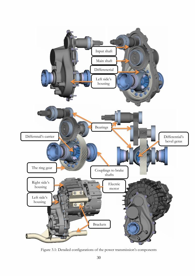
30

Figure 3.1: Detailed configurations of the power transmission’s components

Input shaft

Differenetial

Main shaft

Bearings

Differntail’s carrier

Brackets

Couplings to brake shafts

Electric motor

Right side’s housing

Left side’s housing

Differential’s bevel geras

Left side’s housing

The ring gear

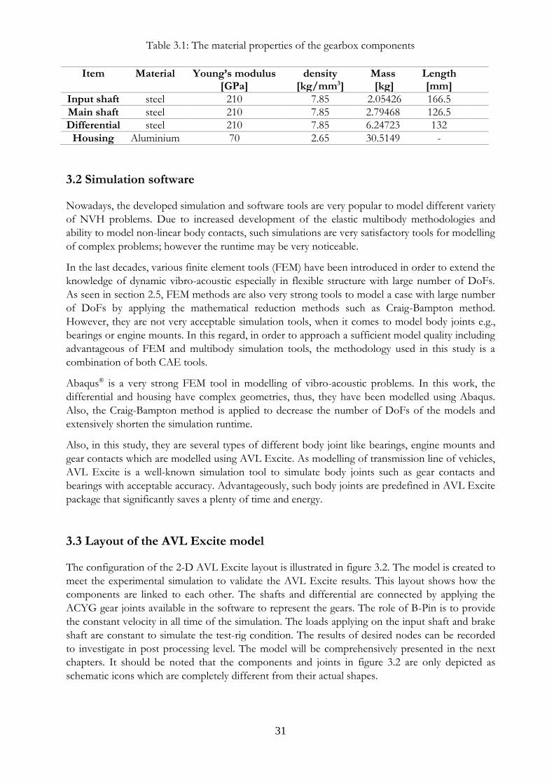
31

Table 3.1: The material properties of the gearbox components

3.2 Simulation software Nowadays, the developed simulation and software tools are very popular to model different variety

of NVH problems. Due to increased development of the elastic multibody methodologies and

ability to model non-linear body contacts, such simulations are very satisfactory tools for modelling

of complex problems; however the runtime may be very noticeable.

In the last decades, various finite element tools (FEM) have been introduced in order to extend the

knowledge of dynamic vibro-acoustic especially in flexible structure with large number of DoFs.

As seen in section 2.5, FEM methods are also very strong tools to model a case with large number

of DoFs by applying the mathematical reduction methods such as Craig-Bampton method.

However, they are not very acceptable simulation tools, when it comes to model body joints e.g.,

bearings or engine mounts. In this regard, in order to approach a sufficient model quality including

advantageous of FEM and multibody simulation tools, the methodology used in this study is a

combination of both CAE tools.

Abaqus® is a very strong FEM tool in modelling of vibro-acoustic problems. In this work, the

differential and housing have complex geometries, thus, they have been modelled using Abaqus.

Also, the Craig-Bampton method is applied to decrease the number of DoFs of the models and

extensively shorten the simulation runtime.

Also, in this study, they are several types of different body joint like bearings, engine mounts and

gear contacts which are modelled using AVL Excite. As modelling of transmission line of vehicles,

AVL Excite is a well-known simulation tool to simulate body joints such as gear contacts and

bearings with acceptable accuracy. Advantageously, such body joints are predefined in AVL Excite

package that significantly saves a plenty of time and energy.

3.3 Layout of the AVL Excite model The configuration of the 2-D AVL Excite layout is illustrated in figure 3.2. The model is created to

meet the experimental simulation to validate the AVL Excite results. This layout shows how the

components are linked to each other. The shafts and differential are connected by applying the

ACYG gear joints available in the software to represent the gears. The role of B-Pin is to provide

the constant velocity in all time of the simulation. The loads applying on the input shaft and brake

shaft are constant to simulate the test-rig condition. The results of desired nodes can be recorded

to investigate in post processing level. The model will be comprehensively presented in the next

chapters. It should be noted that the components and joints in figure 3.2 are only depicted as

schematic icons which are completely different from their actual shapes.

Item Material Young’s modulus [GPa]

density [kg/mm3]

Mass [kg]

Length [mm]

Input shaft steel 210 7.85 2.05426 166.5

Main shaft steel 210 7.85 2.79468 126.5

Differential steel 210 7.85 6.24723 132

Housing Aluminium 70 2.65 30.5149 -

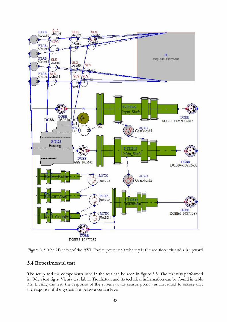
32

3.4 Experimental test The setup and the components used in the test can be seen in figure 3.3. The test was performed in Oden test rig at Vicura test lab in Trollhättan and its technical information can be found in table 3.2. During the test, the response of the system at the sensor point was measured to ensure that the response of the system is a below a certain level.

Figure 3.2: The 2D view of the AVL Excite power unit where y is the rotation axis and z is upward

33

In this test, the original brackets with rubber bushing were used which were screwed on the gearbox and then placed in right position for the test run by supporting fixture. The gearbox is suspended with rubber bushings pressed on the supporting fixture. Also, three accelerometers were assembled on a square block to allow for tri-axial measurement up to 10 kHz, see figure 3.4. The accelerometer block was then attached to the housing with X-60. The accelerometer was mounted on the gearbox near to the differential.

Table 3.2: The technical information of the test

Additional analysis information

All data acquired with a sampling rate of 25600 Hz

Speed signal 1024 pulses on the output shaft

FFT Bandwidth 10 kHz

FFT Block size 4096

Window Hanning

Amplitude Peak

Waterfall data for all individual accelerometer signals

Order bandwidth 0.5 order

Calculations

The vector sum of the 3 directions, X, Y, Z, was used as input and output for the fundamental and harmonics for all load conditions.

An average of the levels of the vector sums of the fundamentals and harmonics of tooth meshing rates over the measured speed range for drive and recuperation of the input and output gears.

Input gear orders: Fundamental order 29 relative input rpm 1st harmonic order 58 relative input rpm

Output gear orders: Fundamental order 80 relative output rpm 1st harmonic order 160 relative output rpm 2nd harmonic order 240 relative output rpm

Test rig setup

2-motor test rig

Original E-Motor driven in torque control

One motor was used in speed control mode on the side shaft. On input shaft, another electrical motor was used in torque control mode

Output with torque and speed measurement

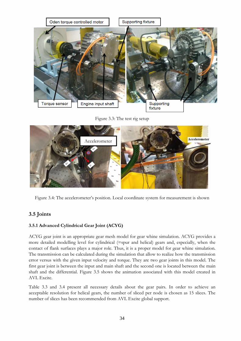
34

Figure 3.3: The test rig setup

Figure 3.4: The accelerometer’s position. Local coordinate system for measurement is shown

3.5 Joints 3.5.1 Advanced Cylindrical Gear Joint (ACYG) ACYG gear joint is an appropriate gear mesh model for gear whine simulation. ACYG provides a

more detailed modelling level for cylindrical (=spur and helical) gears and, especially, when the

contact of flank surfaces plays a major role. Thus, it is a proper model for gear whine simulation.

The transmission can be calculated during the simulation that allow to realize how the transmission

error versus with the given input velocity and torque. They are two gear joints in this model. The

first gear joint is between the input and main shaft and the second one is located between the main

shaft and the differential. Figure 3.5 shows the animation associated with this model created in

AVL Excite.

Table 3.3 and 3.4 present all necessary details about the gear pairs. In order to achieve an

acceptable resolution for helical gears, the number of sliced per node is chosen as 15 slices. The

number of slices has been recommended from AVL Excite global support.

Accelerometer

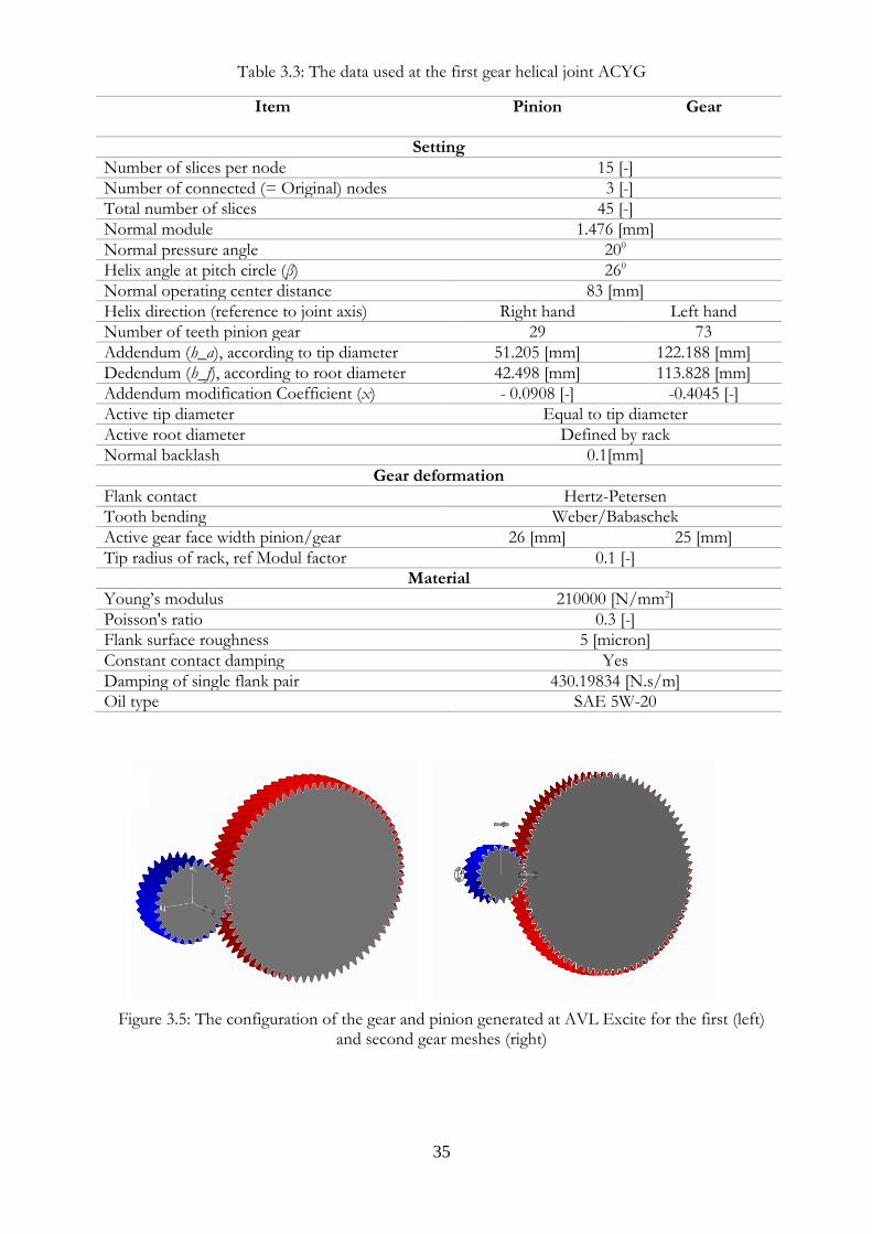
35

Table 3.3: The data used at the first gear helical joint ACYG

Item Pinion Gear

Setting

Number of slices per node 15 [-]

Number of connected (= Original) nodes 3 [-]

Total number of slices 45 [-]

Normal module 1.476 [mm]

Normal pressure angle 200

Helix angle at pitch circle (β) 260

Normal operating center distance 83 [mm]

Helix direction (reference to joint axis) Right hand Left hand

Number of teeth pinion gear 29 73

Addendum (h_a), according to tip diameter 51.205 [mm] 122.188 [mm]

Dedendum (h_f), according to root diameter 42.498 [mm] 113.828 [mm]

Addendum modification Coefficient (x) - 0.0908 [-] -0.4045 [-]

Active tip diameter Equal to tip diameter

Active root diameter Defined by rack

Normal backlash 0.1[mm]

Gear deformation

Flank contact Hertz-Petersen

Tooth bending Weber/Babaschek

Active gear face width pinion/gear 26 [mm] 25 [mm]

Tip radius of rack, ref Modul factor 0.1 [-]

Material

Young’s modulus 210000 [N/mm2]

Poisson's ratio 0.3 [-]

Flank surface roughness 5 [micron]

Constant contact damping Yes

Damping of single flank pair 430.19834 [N.s/m]

Oil type SAE 5W-20

Figure 3.5: The configuration of the gear and pinion generated at AVL Excite for the first (left) and second gear meshes (right)

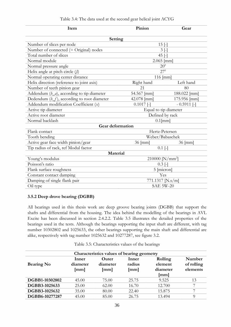
36

Table 3.4: The data used at the second gear helical joint ACYG

Item Pinion Gear

Setting

Number of slices per node 15 [-]

Number of connected (= Original) nodes 3 [-]

Total number of slices 45 [-]

Normal module 2.065 [mm]

Normal pressure angle 200

Helix angle at pitch circle (β) 270

Normal operating center distance 116 [mm]

Helix direction (reference to joint axis) Right hand Left hand

Number of teeth pinion gear 21 80

Addendum (h_a), according to tip diameter 54.567 [mm] 188.022 [mm]

Dedendum (h_f ), according to root diameter 42.078 [mm] 175.956 [mm]

Addendum modification Coefficient (x) 0.1017 [-] - 0.5911 [-]

Active tip diameter Equal to tip diameter

Active root diameter Defined by rack

Normal backlash 0.1[mm]

Gear deformation

Flank contact Hertz-Petersen

Tooth bending Weber/Babaschek

Active gear face width pinion/gear 36 [mm] 36 [mm]

Tip radius of rack, ref Modul factor 0.1 [-]

Material

Young’s modulus 210000 [N/mm2]

Poisson's ratio 0.3 [-]

Flank surface roughness 5 [micron]

Constant contact damping Yes

Damping of single flank pair 771.1317 [N.s/m]

Oil type SAE 5W-20

3.5.2 Deep drove bearing (DGBB) All bearings used in this thesis work are deep groove bearing joints (DGBB) that support the

shafts and differential from the housing. The idea behind the modelling of the bearings in AVL

Excite has been discussed in section 2.4.2.2. Table 3.5 illustrates the detailed properties of the

bearings used in the tests. Although the bearings supporting the input shaft are different, with tag

number 10302802 and 1025633, the other bearings supporting the main shaft and differential are

alike, respectively with tag number 1025632 and 10277287, see figure 3.2.

Table 3.5: Characteristics values of the bearings

Characteristics values of bearing geometry

Bearing No

Inner diameter

[mm]

Outer diameter

[mm]

Inner radius [mm]

Rolling element diameter

[mm]

Number of rolling elements

DGBB1-10302802 45.00 75.00 25.75 9.525 13

DGBB3-1025633 25.00 62.00 16.70 12.700 7

DGBB3-1025632 35.00 80.00 22.40 15.875 7

DGBB6-10277287 45.00 85.00 26.75 13.494 9

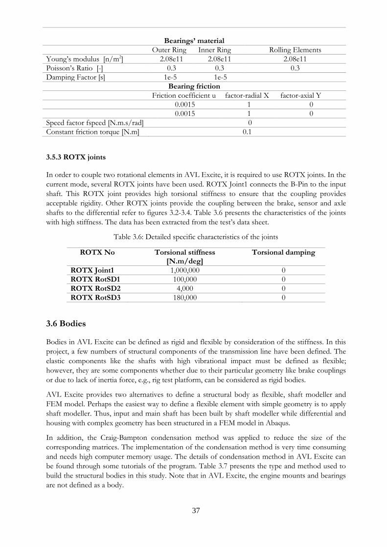
37

Bearings’ material

Outer Ring Inner Ring Rolling Elements

Young’s modulus [n/m2] 2.08e11 2.08e11 2.08e11

Poisson’s Ratio [-] 0.3 0.3 0.3

Damping Factor [s] 1e-5 1e-5

Bearing friction

Friction coefficient u factor-radial X factor-axial Y

0.0015 1 0

0.0015 1 0

Speed factor fspeed [N.m.s/rad] 0

Constant friction torque [N.m] 0.1

3.5.3 ROTX joints In order to couple two rotational elements in AVL Excite, it is required to use ROTX joints. In the

current mode, several ROTX joints have been used. ROTX Joint1 connects the B-Pin to the input

shaft. This ROTX joint provides high torsional stiffness to ensure that the coupling provides

acceptable rigidity. Other ROTX joints provide the coupling between the brake, sensor and axle

shafts to the differential refer to figures 3.2-3.4. Table 3.6 presents the characteristics of the joints

with high stiffness. The data has been extracted from the test’s data sheet.

Table 3.6: Detailed specific characteristics of the joints

ROTX No Torsional stiffness [N.m/deg]

Torsional damping

ROTX Joint1 1,000,000 0

ROTX RotSD1 100,000 0

ROTX RotSD2 4,000 0

ROTX RotSD3 180,000 0

3.6 Bodies Bodies in AVL Excite can be defined as rigid and flexible by consideration of the stiffness. In this

project, a few numbers of structural components of the transmission line have been defined. The

elastic components like the shafts with high vibrational impact must be defined as flexible;

however, they are some components whether due to their particular geometry like brake couplings

or due to lack of inertia force, e.g., rig test platform, can be considered as rigid bodies.

AVL Excite provides two alternatives to define a structural body as flexible, shaft modeller and

FEM model. Perhaps the easiest way to define a flexible element with simple geometry is to apply

shaft modeller. Thus, input and main shaft has been built by shaft modeller while differential and

housing with complex geometry has been structured in a FEM model in Abaqus.

In addition, the Craig-Bampton condensation method was applied to reduce the size of the

corresponding matrices. The implementation of the condensation method is very time consuming

and needs high computer memory usage. The details of condensation method in AVL Excite can

be found through some tutorials of the program. Table 3.7 presents the type and method used to

build the structural bodies in this study. Note that in AVL Excite, the engine mounts and bearings

are not defined as a body.

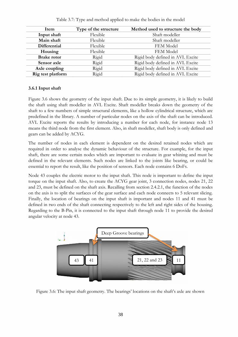
38

Table 3.7: Type and method applied to make the bodies in the model

Item Type of the structure Method used to structure the body

Input shaft Flexible Shaft modeller

Main shaft Flexible Shaft modeller

Differential Flexible FEM Model

Housing Flexible FEM Model

Brake rotor Rigid Rigid body defined in AVL Excite

Sensor axle Rigid Rigid body defined in AVL Excite

Axle coupling Rigid Rigid body defined in AVL Excite

Rig test platform Rigid Rigid body defined in AVL Excite

3.6.1 Input shaft Figure 3.6 shows the geometry of the input shaft. Due to its simple geometry, it is likely to build

the shaft using shaft modeller in AVL Excite. Shaft modeller breaks down the geometry of the

shaft to a few numbers of simple structural elements, like a hollow cylindrical structure, which are

predefined in the library. A number of particular nodes on the axis of the shaft can be introduced.

AVL Excite reports the results by introducing a number for each node, for instance node 13

means the third node from the first element. Also, in shaft modeller, shaft body is only defined and

gears can be added by ACYG.

The number of nodes in each element is dependent on the desired retained nodes which are

required in order to analyse the dynamic behaviour of the structure. For example, for the input

shaft, there are some certain nodes which are important to evaluate in gear whining and must be

defined in the relevant elements. Such nodes are linked to the joints like bearing, or could be

essential to report the result, like the position of sensors. Each node contains 6 DoFs.

Node 43 couples the electric motor to the input shaft. This node is important to define the input

torque on the input shaft. Also, to create the ACYG gear joint, 3 connection nodes, nodes 21, 22

and 23, must be defined on the shaft axis. Recalling from section 2.4.2.1, the function of the nodes

on the axis is to split the surfaces of the gear surface and each node connects to 5 relevant slicing.

Finally, the location of bearings on the input shaft is important and nodes 11 and 41 must be

defined in two ends of the shaft connecting respectively to the left and right sides of the housing.

Regarding to the B-Pin, it is connected to the input shaft through node 11 to provide the desired

angular velocity at node 43.

21, 22 and 23 43 41 11

Figure 3.6: The input shaft geometry. The bearings’ locations on the shaft’s axle are shown

Deep Groove bearings location

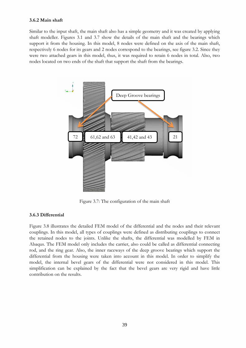
39

3.6.2 Main shaft Similar to the input shaft, the main shaft also has a simple geometry and it was created by applying

shaft modeller. Figures 3.1 and 3.7 show the details of the main shaft and the bearings which

support it from the housing. In this model, 8 nodes were defined on the axis of the main shaft,

respectively 6 nodes for its gears and 2 nodes correspond to the bearings, see figure 3.2. Since they

were two attached gears in this model, thus, it was required to retain 6 nodes in total. Also, two

nodes located on two ends of the shaft that support the shaft from the bearings.

Figure 3.7: The configuration of the main shaft

3.6.3 Differential Figure 3.8 illustrates the detailed FEM model of the differential and the nodes and their relevant

couplings. In this model, all types of couplings were defined as distributing couplings to connect

the retained nodes to the joints. Unlike the shafts, the differential was modelled by FEM in

Abaqus. The FEM model only includes the carrier, also could be called as differential connecting

rod, and the ring gear. Also, the inner raceways of the deep groove bearings which support the

differential from the housing were taken into account in this model. In order to simplify the

model, the internal bevel gears of the differential were not considered in this model. This

simplification can be explained by the fact that the bevel gears are very rigid and have little

contribution on the results.

41,42 and 43 61,62 and 63 21 72

Deep Groove bearings location

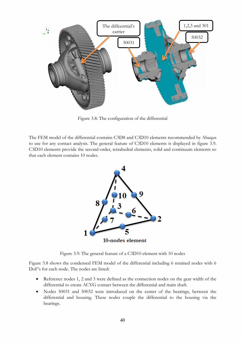
40

Figure 3.8: The configuration of the differential

The FEM model of the differential contains C3D8 and C3D10 elements recommended by Abaqus

to use for any contact analysis. The general feature of C3D10 elements is displayed in figure 3.9.

C3D10 elements provide the second-order, tetrahedral elements, solid and continuum elements so

that each element contains 10 nodes.

Figure 3.9: The general feature of a C3D10 element with 10 nodes

Figure 3.8 shows the condensed FEM model of the differential including 6 retained nodes with 6

DoF’s for each node. The nodes are listed:

• Reference nodes 1, 2 and 3 were defined as the connection nodes on the gear width of the

differential to create ACYG contact between the differential and main shaft.

• Nodes 50031 and 50032 were introduced on the center of the bearings, between the

differential and housing. These nodes couple the differential to the housing via the

bearings.

1,2,3 and 301

50032 50031

The diffeenrtial’s carrier

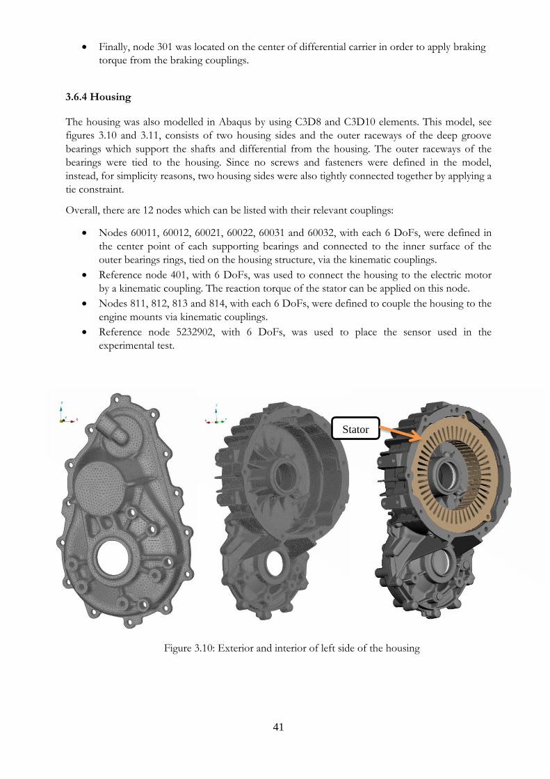
41

• Finally, node 301 was located on the center of differential carrier in order to apply braking

torque from the braking couplings.

3.6.4 Housing The housing was also modelled in Abaqus by using C3D8 and C3D10 elements. This model, see

figures 3.10 and 3.11, consists of two housing sides and the outer raceways of the deep groove

bearings which support the shafts and differential from the housing. The outer raceways of the

bearings were tied to the housing. Since no screws and fasteners were defined in the model,

instead, for simplicity reasons, two housing sides were also tightly connected together by applying a

tie constraint.

Overall, there are 12 nodes which can be listed with their relevant couplings:

• Nodes 60011, 60012, 60021, 60022, 60031 and 60032, with each 6 DoFs, were defined in

the center point of each supporting bearings and connected to the inner surface of the

outer bearings rings, tied on the housing structure, via the kinematic couplings.

• Reference node 401, with 6 DoFs, was used to connect the housing to the electric motor

by a kinematic coupling. The reaction torque of the stator can be applied on this node.

• Nodes 811, 812, 813 and 814, with each 6 DoFs, were defined to couple the housing to the

engine mounts via kinematic couplings.

• Reference node 5232902, with 6 DoFs, was used to place the sensor used in the

experimental test.

Figure 3.10: Exterior and interior of left side of the housing

Stator

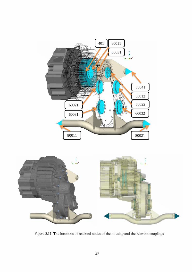
42

401

60012

60032 60031

80031

60022 60021

80041

60011

80011 80021

Figure 3.11: The locations of retained nodes of the housing and the relevant couplings

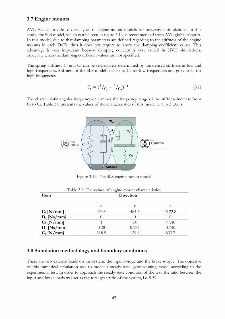
43

3.7 Engine mounts AVL Excite provides diverse types of engine mount models for powertrain simulations. In this study, the SLS model, which can be seen in figure 3.12, is recommended from AVL global support. In this model, due to that damping parameters are defined regarding to the stiffness of the engine mounts in each DoFs, thus it does not require to know the damping coefficient values. This advantage is very important because damping concept is very crucial in NVH simulations, especially when the damping coefficient values are not specified. The spring stiffness C1 and C2 can be respectively determined by the desired stiffness at low and high frequencies. Stiffness of the SLS model is close to Cs for low frequencies and goes to C2 for high frequencies.

𝐶𝑠 = (1𝐶1

⁄ + 1𝐶2

⁄ )−1 (3.1)

The characteristic angular frequency determines the frequency range of the stiffness increase from C1 to C2. Table 3.8 presents the values of the characteristics of this model at 1 to 3 DoFs.

Figure 3.12: The SLS engine mount model

Table 3.8: The values of engine mount characteristics

Item Direction

x y z

C1 [N/mm] 1225 464.5 3122.8

D1 [Ns/mm] 0 0 0

C2 [N/mm] 1 1.0 47.40

D2 [Ns/mm] 0.28 0.124 0.740

C3 [N/mm] 318.5 129.8 833.7

3.8 Simulation methodology and boundary conditions There are two external loads on the system; the input torque and the brake torque. The objective

of this numerical simulation was to model a steady-state, gear whining model according to the

experimental test. In order to approach the steady-state condition of the test, the ratio between the

input and brake loads was set as the total gear ratio of the system, i.e. 9.59.

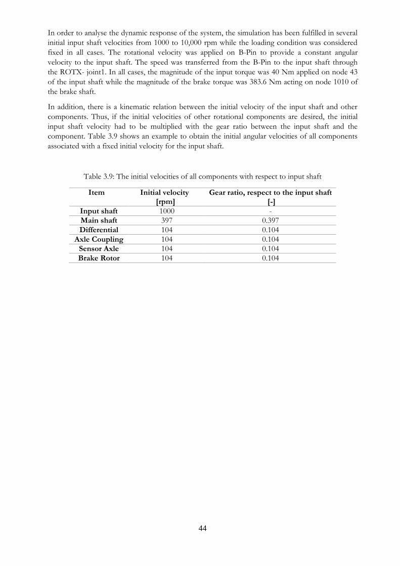
44

In order to analyse the dynamic response of the system, the simulation has been fulfilled in several

initial input shaft velocities from 1000 to 10,000 rpm while the loading condition was considered

fixed in all cases. The rotational velocity was applied on B-Pin to provide a constant angular

velocity to the input shaft. The speed was transferred from the B-Pin to the input shaft through

the ROTX- joint1. In all cases, the magnitude of the input torque was 40 Nm applied on node 43

of the input shaft while the magnitude of the brake torque was 383.6 Nm acting on node 1010 of

the brake shaft.

In addition, there is a kinematic relation between the initial velocity of the input shaft and other

components. Thus, if the initial velocities of other rotational components are desired, the initial

input shaft velocity had to be multiplied with the gear ratio between the input shaft and the

component. Table 3.9 shows an example to obtain the initial angular velocities of all components

associated with a fixed initial velocity for the input shaft.

Table 3.9: The initial velocities of all components with respect to input shaft

Item Initial velocity [rpm]

Gear ratio, respect to the input shaft [-]

Input shaft 1000 -

Main shaft 397 0.397

Differential 104 0.104

Axle Coupling 104 0.104

Sensor Axle 104 0.104

Brake Rotor 104 0.104

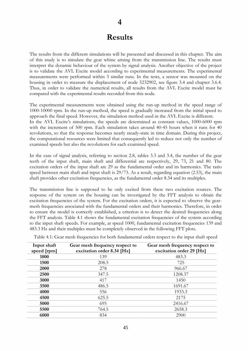
45

4

Results

The results from the different simulations will be presented and discussed in this chapter. The aim of this study is to simulate the gear whine arising from the transmission line. The results must interpret the dynamic behaviour of the system by signal analysis. Another objective of the project is to validate the AVL Excite model according to experimental measurements. The experimental measurements were performed within 3 similar runs. In the tests, a sensor was mounted on the housing in order to measure the displacement of node 5232902, see figure 3.4 and chapter 3.6.4. Thus, in order to validate the numerical results, all results from the AVL Excite model must be compared with the experimental results recorded from this node. The experimental measurements were obtained using the run-up method in the speed range of 1000-10000 rpm. In the run-up method, the speed is gradually increased from the initial speed to approach the final speed. However, the simulation method used in the AVL Excite is different. In the AVL Excite’s simulations, the speeds are determined as constant values, 1000-6000 rpm with the increment of 500 rpm. Each simulation takes around 40-45 hours when it runs for 40 revolutions, so that the response becomes nearly steady-state in time domain. During this project, the computational resources were limited that consequently led to reduce not only the number of examined speeds but also the revolutions for each examined speed. In the case of signal analysis, referring to section 2.8, tables 3.3 and 3.4, the number of the gear teeth of the input shaft, main shaft and differential are respectively, 29, 73, 21 and 80. The excitation orders of the input shaft are 29 as the fundamental order and its harmonics. The ratio speed between main shaft and input shaft is 29/73. As a result, regarding equation (2.53), the main shaft provides other excitation frequencies, as the fundamental order 8.34 and its multiples. The transmission line is supposed to be only excited from these two excitation sources. The response of the system on the housing can be investigated by the FFT analysis to obtain the excitation frequencies of the system. For the excitation orders, it is expected to observe the gear-mesh frequencies associated with the fundamental orders and their harmonics. Therefore, in order to ensure the model is correctly established, a criterion is to detect the desired frequencies along the FFT analysis. Table 4.1 shows the fundamental excitation frequencies of the system according to the input shaft speeds. For example, at speed 1000, fundamental excitation frequencies 139 and 483.3 Hz and their multiples must be completely observed in the following FFT plots.

Table 4.1: Gear mesh frequencies for both fundamental orders respect to the input shaft speed

Input shaft speed [rpm]

Gear mesh frequency respect to excitation order 8.34 [Hz]

Gear mesh frequency respect to excitation order 29 [Hz]

1000 139 483.3

1500 208.5 725

2000 278 966.67

2500 347.5 1208.37

3000 417 1450

3500 486.5 1691.67

4000 556 1933.3

4500 625.5 2175

5000 695 2416.67

5500 764.5 2658.3

6000 834 2900

46

Overall, the damping coefficient for each flexible mechanical component is a critical challenge in NVH analysis. Thus, another objective of this work is to detect how the damping parameter contributes on the response of the system. There are diverse useful models of the engine mounts in AVL Excite. In this project, as discussed in section 3.7, damping parameters of the engine mounts in all directions were determined based on the stiffness. Consequently, as an advantage, the exact values of engine mounts’ damping coefficients were not necessary to be specified. Except the engine mounts, for other mechanical components, the shafts, bearings, gears and housing, the damping coefficients have not been chosen with certainty. These values have been initially determined according to similar projects fulfilled at AVL Vicura, see table 4.3. The uncertainty of the system parameters, such as damping coefficient or bearing stiffness, may dramatically lead to noticeable discrepancies between the experimental and the AVL Excite’s results. Thus, due to the key role of damping, a sensitivity analysis on damping reduction for these components will be performed to obtain which component would provide the highest effect on the dynamic response.

4.1 The simulation results from the AVL Excite model In all simulations, the loading conditions are similar providing the steady-state conditions described

in section 3.8. Node 5232902 is a reference node with great of importance in order to compare the

numerical and experimental results together and analyse the dynamic response of the system. AVL

Excite totally reports the dynamic behaviours of all components. However, in order to compare

with the experimental results which are only available in this node, almost all results have been

reported on this node. Additionally, as previously discussed, uncertainty of the damping

coefficients as well as the stiffness of other components (e.g., bearings) may result in some

discrepancies.

Figure 4.1 shows the dynamic angular transmission error and mesh stiffness, of the gear pair 1 and

2 at speed 1000 rpm in the last mesh cycles. The results are nearly steady-state after 40 cycles. In

order to compare the static transmission error from the AVL Excite model to other programs like

LDP (the Load Distribution Program), it seems that some modifications on the gear mesh model

are required. In this study, the results from LDP were available for the gears; however, because of

lack of time, the modifications on the gear pairs were not performed.

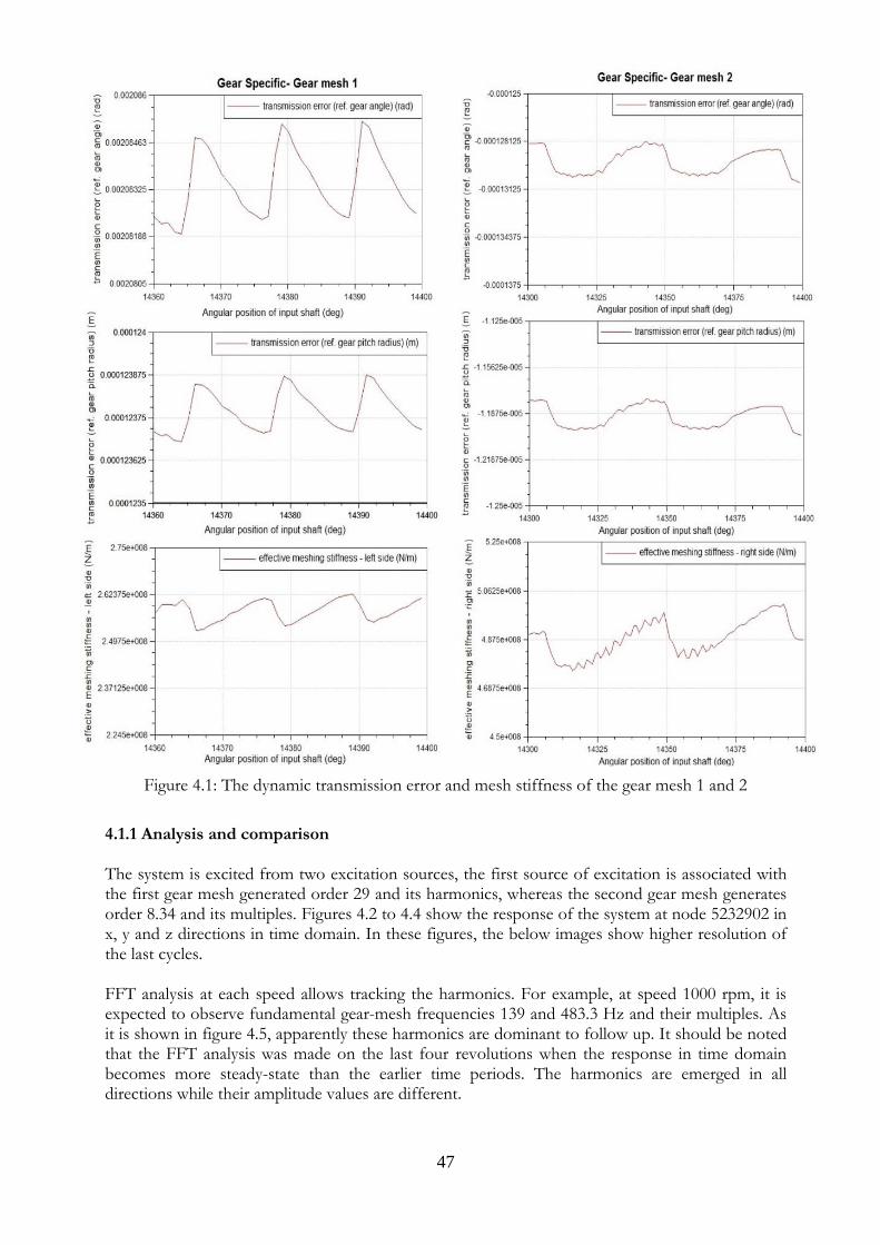
47

4.1.1 Analysis and comparison The system is excited from two excitation sources, the first source of excitation is associated with the first gear mesh generated order 29 and its harmonics, whereas the second gear mesh generates order 8.34 and its multiples. Figures 4.2 to 4.4 show the response of the system at node 5232902 in x, y and z directions in time domain. In these figures, the below images show higher resolution of the last cycles. FFT analysis at each speed allows tracking the harmonics. For example, at speed 1000 rpm, it is expected to observe fundamental gear-mesh frequencies 139 and 483.3 Hz and their multiples. As it is shown in figure 4.5, apparently these harmonics are dominant to follow up. It should be noted that the FFT analysis was made on the last four revolutions when the response in time domain becomes more steady-state than the earlier time periods. The harmonics are emerged in all directions while their amplitude values are different.

Figure 4.1: The dynamic transmission error and mesh stiffness of the gear mesh 1 and 2

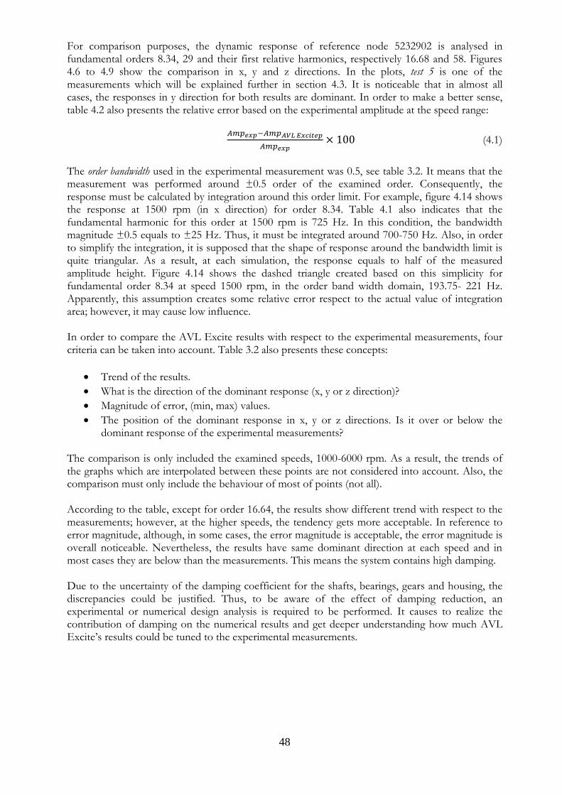
48

For comparison purposes, the dynamic response of reference node 5232902 is analysed in fundamental orders 8.34, 29 and their first relative harmonics, respectively 16.68 and 58. Figures 4.6 to 4.9 show the comparison in x, y and z directions. In the plots, test 5 is one of the measurements which will be explained further in section 4.3. It is noticeable that in almost all cases, the responses in y direction for both results are dominant. In order to make a better sense, table 4.2 also presents the relative error based on the experimental amplitude at the speed range:

𝐴𝑚𝑝𝑒𝑥𝑝−𝐴𝑚𝑝𝐴𝑉𝐿 𝐸𝑥𝑐𝑖𝑡𝑒𝑝

𝐴𝑚𝑝𝑒𝑥𝑝× 100 (4.1)

The order bandwidth used in the experimental measurement was 0.5, see table 3.2. It means that the measurement was performed around ±0.5 order of the examined order. Consequently, the response must be calculated by integration around this order limit. For example, figure 4.14 shows the response at 1500 rpm (in x direction) for order 8.34. Table 4.1 also indicates that the fundamental harmonic for this order at 1500 rpm is 725 Hz. In this condition, the bandwidth magnitude ±0.5 equals to ±25 Hz. Thus, it must be integrated around 700-750 Hz. Also, in order to simplify the integration, it is supposed that the shape of response around the bandwidth limit is quite triangular. As a result, at each simulation, the response equals to half of the measured amplitude height. Figure 4.14 shows the dashed triangle created based on this simplicity for fundamental order 8.34 at speed 1500 rpm, in the order band width domain, 193.75- 221 Hz. Apparently, this assumption creates some relative error respect to the actual value of integration area; however, it may cause low influence. In order to compare the AVL Excite results with respect to the experimental measurements, four criteria can be taken into account. Table 3.2 also presents these concepts:

• Trend of the results.

• What is the direction of the dominant response (x, y or z direction)?

• Magnitude of error, (min, max) values.

• The position of the dominant response in x, y or z directions. Is it over or below the dominant response of the experimental measurements?

The comparison is only included the examined speeds, 1000-6000 rpm. As a result, the trends of the graphs which are interpolated between these points are not considered into account. Also, the comparison must only include the behaviour of most of points (not all). According to the table, except for order 16.64, the results show different trend with respect to the measurements; however, at the higher speeds, the tendency gets more acceptable. In reference to error magnitude, although, in some cases, the error magnitude is acceptable, the error magnitude is overall noticeable. Nevertheless, the results have same dominant direction at each speed and in most cases they are below than the measurements. This means the system contains high damping. Due to the uncertainty of the damping coefficient for the shafts, bearings, gears and housing, the discrepancies could be justified. Thus, to be aware of the effect of damping reduction, an experimental or numerical design analysis is required to be performed. It causes to realize the contribution of damping on the numerical results and get deeper understanding how much AVL Excite’s results could be tuned to the experimental measurements.

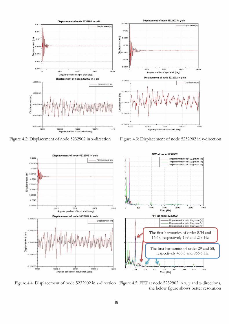
49

Figure 4.2: Displacement of node 5232902 in x-direction Figure 4.3: Displacement of node 5232902 in y-direction

Figure 4.4: Displacement of node 5232902 in z-direction Figure 4.5: FFT at node 5232902 in x, y and z-directions,

the below figure shows better resolution

The first harmonics of order 8.34 and 16.68, respectively 139 and 278 Hz

The first harmonics of order 29 and 58, respectively 483.3 and 966.6 Hz

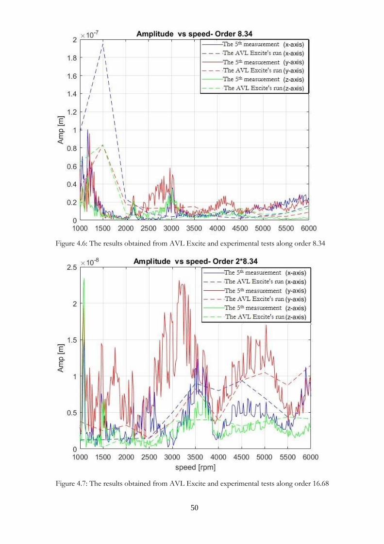
50

Figure 4.7: The results obtained from AVL Excite and experimental tests along order 16.68

Figure 4.6: The results obtained from AVL Excite and experimental tests along order 8.34

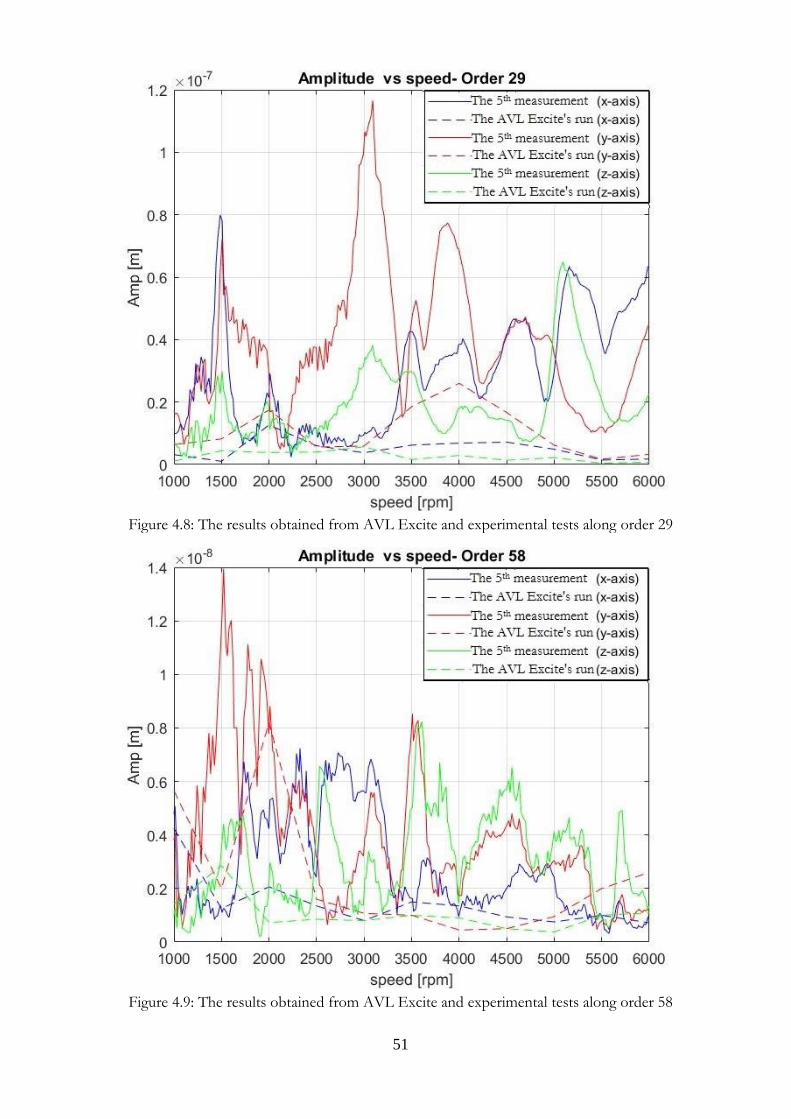
51

Figure 4.8: The results obtained from AVL Excite and experimental tests along order 29

Figure 4.9: The results obtained from AVL Excite and experimental tests along order 58

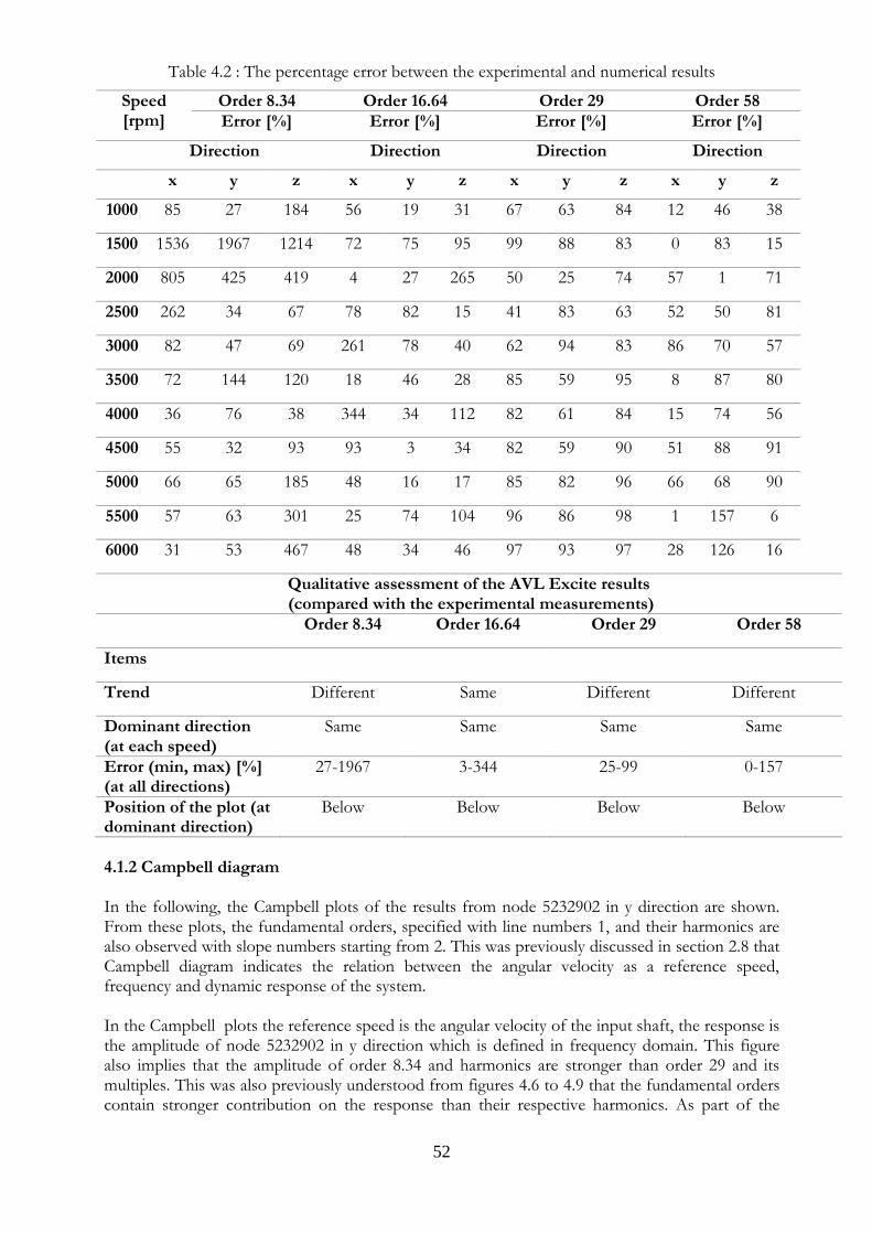
52

Table 4.2 : The percentage error between the experimental and numerical results

Speed [rpm]

Order 8.34 Order 16.64 Order 29 Order 58

Error [%] Error [%] Error [%] Error [%]

Direction Direction Direction Direction

x y z x y z x y z x y z

1000 85 27 184 56 19 31 67 63 84 12 46 38

1500 1536 1967 1214 72 75 95 99 88 83 0 83 15

2000 805 425 419 4 27 265 50 25 74 57 1 71

2500 262 34 67 78 82 15 41 83 63 52 50 81

3000 82 47 69 261 78 40 62 94 83 86 70 57

3500 72 144 120 18 46 28 85 59 95 8 87 80

4000 36 76 38 344 34 112 82 61 84 15 74 56

4500 55 32 93 93 3 34 82 59 90 51 88 91

5000 66 65 185 48 16 17 85 82 96 66 68 90

5500 57 63 301 25 74 104 96 86 98 1 157 6

6000 31 53 467 48 34 46 97 93 97 28 126 16

Qualitative assessment of the AVL Excite results (compared with the experimental measurements)

Order 8.34 Order 16.64 Order 29 Order 58

Items

Trend Different Same Different Different

Dominant direction (at each speed)

Same Same Same Same

Error (min, max) [%] (at all directions)

27-1967 3-344 25-99 0-157

Position of the plot (at dominant direction)

Below Below Below Below

4.1.2 Campbell diagram In the following, the Campbell plots of the results from node 5232902 in y direction are shown. From these plots, the fundamental orders, specified with line numbers 1, and their harmonics are also observed with slope numbers starting from 2. This was previously discussed in section 2.8 that Campbell diagram indicates the relation between the angular velocity as a reference speed, frequency and dynamic response of the system. In the Campbell plots the reference speed is the angular velocity of the input shaft, the response is the amplitude of node 5232902 in y direction which is defined in frequency domain. This figure also implies that the amplitude of order 8.34 and harmonics are stronger than order 29 and its multiples. This was also previously understood from figures 4.6 to 4.9 that the fundamental orders contain stronger contribution on the response than their respective harmonics. As part of the

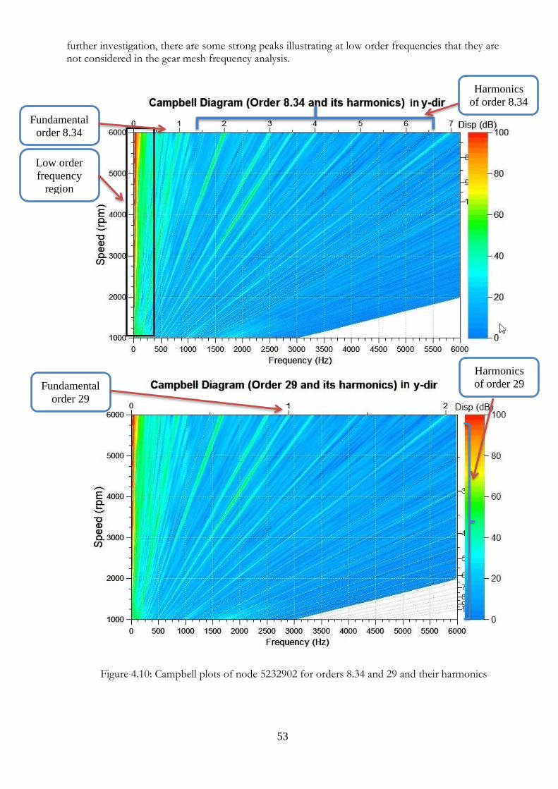
53

further investigation, there are some strong peaks illustrating at low order frequencies that they are not considered in the gear mesh frequency analysis.

Figure 4.10: Campbell plots of node 5232902 for orders 8.34 and 29 and their harmonics

Fundamental

order 8.34

Low order

frequency

region

Fundamental

order 29

Harmonics

of order 8.34

Harmonics

of order 29

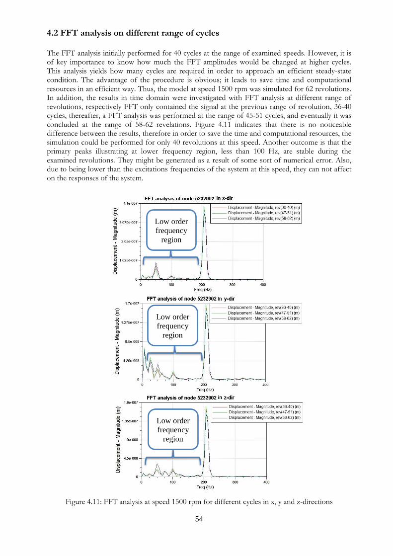
54

4.2 FFT analysis on different range of cycles The FFT analysis initially performed for 40 cycles at the range of examined speeds. However, it is of key importance to know how much the FFT amplitudes would be changed at higher cycles. This analysis yields how many cycles are required in order to approach an efficient steady-state condition. The advantage of the procedure is obvious; it leads to save time and computational resources in an efficient way. Thus, the model at speed 1500 rpm was simulated for 62 revolutions. In addition, the results in time domain were investigated with FFT analysis at different range of revolutions, respectively FFT only contained the signal at the previous range of revolution, 36-40 cycles, thereafter, a FFT analysis was performed at the range of 45-51 cycles, and eventually it was concluded at the range of 58-62 revelations. Figure 4.11 indicates that there is no noticeable difference between the results, therefore in order to save the time and computational resources, the simulation could be performed for only 40 revolutions at this speed. Another outcome is that the primary peaks illustrating at lower frequency region, less than 100 Hz, are stable during the examined revolutions. They might be generated as a result of some sort of numerical error. Also, due to being lower than the excitations frequencies of the system at this speed, they can not affect on the responses of the system.

Figure 4.11: FFT analysis at speed 1500 rpm for different cycles in x, y and z-directions

Low order

frequency

region

Low order

frequency

region

Low order

frequency

region

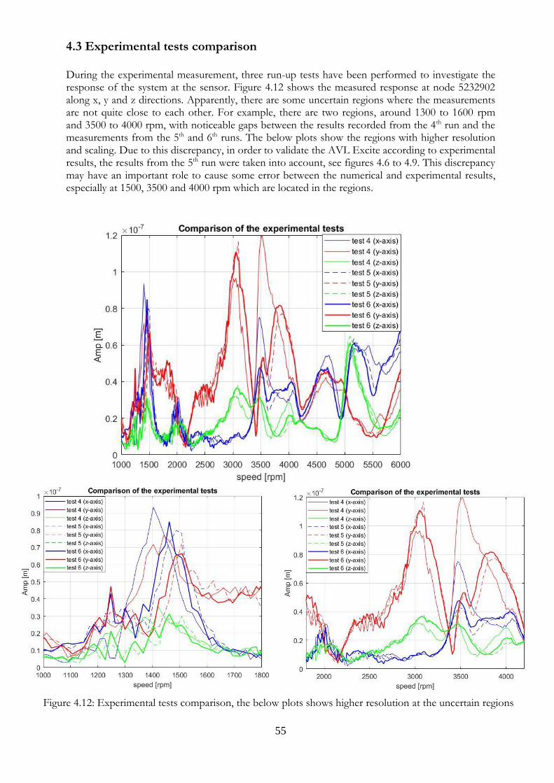
55

4.3 Experimental tests comparison During the experimental measurement, three run-up tests have been performed to investigate the response of the system at the sensor. Figure 4.12 shows the measured response at node 5232902 along x, y and z directions. Apparently, there are some uncertain regions where the measurements are not quite close to each other. For example, there are two regions, around 1300 to 1600 rpm and 3500 to 4000 rpm, with noticeable gaps between the results recorded from the 4th run and the measurements from the 5th and 6th runs. The below plots show the regions with higher resolution and scaling. Due to this discrepancy, in order to validate the AVL Excite according to experimental results, the results from the 5th run were taken into account, see figures 4.6 to 4.9. This discrepancy may have an important role to cause some error between the numerical and experimental results, especially at 1500, 3500 and 4000 rpm which are located in the regions.

Figure 4.12: Experimental tests comparison, the below plots shows higher resolution at the uncertain regions

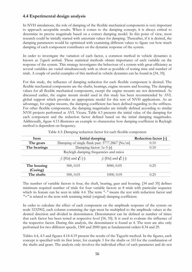
56

4.4 Experimental design analysis In NVH simulations, the role of damping of the flexible mechanical components is very important to approach acceptable results. When it comes to the damping concept, it is always critical to determine its precise magnitude based on a correct damping model. In this point of view, most research could be initially started with uncertain values for damping. Thereafter, if it is desired, the damping parameters would be optimized with examining different values to figure out how much damping of each component contributes on the dynamic response of the system. In order to investigate the variation of each factor, a common method in vehicle dynamics is known as Taguchi methods. These statistical methods obtain importance of each variable on the response of the system. This strategy investigates the behaviour of a system with great efficiency as several variables are varied simultaneously with as short as possible of testing time and number of trials. A couple of useful examples of this method in vehicle dynamics can be found in [34, 35]. For this study, the influence of damping reduction for each flexible component is desired. The flexible mechanical components are the shafts, bearings, engine mounts and housing. The damping values for all flexible mechanical components, except the engine mounts are not determined. As discussed earlier, the engine mount model used in this study has been recommended by AVL global support which provides an appropriate model for this sort of NVH applications. As an advantage, for engine mounts, the damping coefficient has been defined regarding to the stiffness. For other flexible components, the damping magnitudes are initially defined according to similar NVH projects performed at AVL Vicura. Table 4.3 presents the initial value of the damping for each component and the reduction factor defined based on the initial damping magnitudes. Additionally, figure 4.13 illustrates an example to characterize how damping coefficient in Rayleigh method is dependent on frequency.

Table 4.3: Damping reduction factor for each flexible component

Item Initial damping Reduction factor [-]

The gears Damping of single flank pair: 3777.2867 [Ns/m] 0.10

The bearings Damping factor: 1e-5 [s] 0.10

Rayleigh damping frequencies and ratios

f1 [Hz] and 𝜻1 [-]: f2 [Hz] and 𝜻2 [-]:

The housing (Casing)

500, 0.03 3000, 0.05 0.25

The shafts 500, 0.03 1000, 0.05 0.25

The number of variable factors is four, the shaft, bearing, gear and housing. [34 and 35] defines minimum required number of trials for four variable factors as 8 trials with particular sequence which its feature can be seen in table 4.4. The term "–" means the test with reduction factor and "+" is related to the tests with retaining initial (original) damping coefficient. In order to calculate the effect of each component on the amplitude response of the system on node 5232902, each column containing the sign must be multiplied to the amplitude values at the desired direction and divided in denominator. Denominator can be defined as number of times that each factor has been tested at respective level [34, 35]. It is used to evaluate the influence of the respective factor. During this analysis, the denominator is found as 4. The tests are also only performed for two different speeds, 1500 and 2000 rpm at fundamental orders 8.34 and 29. Tables 4.4, 4.5 and figures 4.14-4.19 present the results of the Taguchi method. In the figures, each concept is specified with its first letter, for example S for the shafts or SH for the combination of the shafts and gears. The analysis only involves the individual effect of each parameter and do not

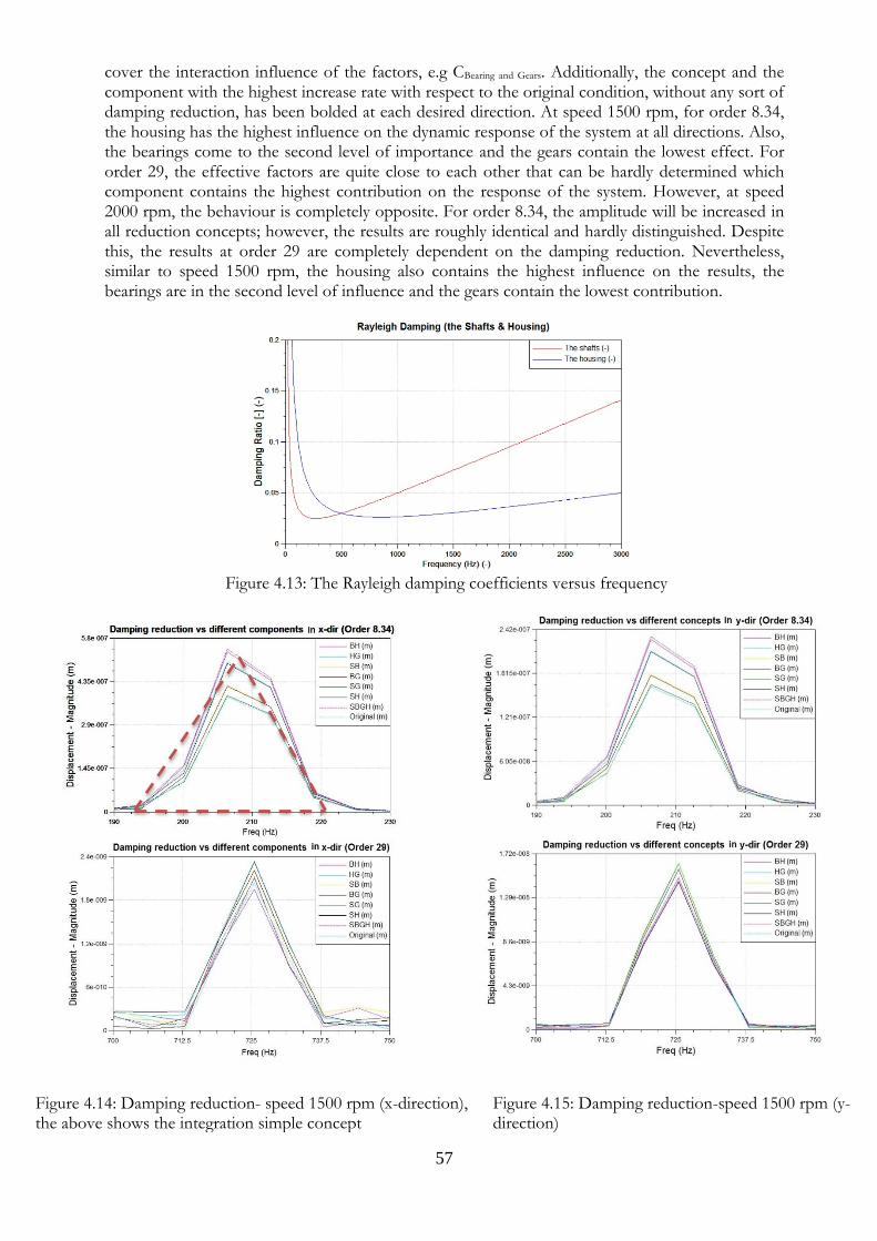
57

cover the interaction influence of the factors, e.g CBearing and Gears. Additionally, the concept and the component with the highest increase rate with respect to the original condition, without any sort of damping reduction, has been bolded at each desired direction. At speed 1500 rpm, for order 8.34, the housing has the highest influence on the dynamic response of the system at all directions. Also, the bearings come to the second level of importance and the gears contain the lowest effect. For order 29, the effective factors are quite close to each other that can be hardly determined which component contains the highest contribution on the response of the system. However, at speed 2000 rpm, the behaviour is completely opposite. For order 8.34, the amplitude will be increased in all reduction concepts; however, the results are roughly identical and hardly distinguished. Despite this, the results at order 29 are completely dependent on the damping reduction. Nevertheless, similar to speed 1500 rpm, the housing also contains the highest influence on the results, the bearings are in the second level of influence and the gears contain the lowest contribution.

Figure 4.13: The Rayleigh damping coefficients versus frequency

Figure 4.14: Damping reduction- speed 1500 rpm (x-direction), the above shows the integration simple concept

Figure 4.15: Damping reduction-speed 1500 rpm (y- direction)

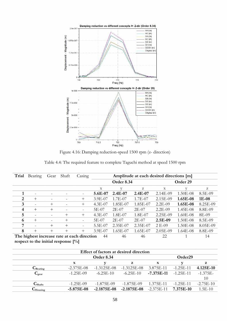
58

Figure 4.16: Damping reduction-speed 1500 rpm (z- direction)

Table 4.4: The required feature to complete Taguchi method at speed 1500 rpm

Trial Bearing Gear Shaft Casing Amplitude at each desired directions [m]

Order 8.34 Order 29

x y z x y z

1 - - - - 5.6E-07 2.4E-07 2.4E-07 2.14E-09 1.50E-08 8.5E-09

2 + - - + 3.9E-07 1.7E-07 1.7E-07 2.15E-09 1.65E-08 1E-08

3 - + - + 4.3E-07 1.85E-07 1.85E-07 2.2E-09 1.65E-08 8.25E-09

4 + + - - 5E-07 2E-07 2E-07 2.2E-09 1.45E-08 8.8E-09

5 - - + + 4.3E-07 1.8E-07 1.8E-07 2.25E-09 1.60E-08 8E-09

6 + - + - 5E-07 2E-07 2E-07 2.5E-09 1.50E-08 8.5E-09

7 - + + - 5.5E-07 2.35E-07 2.35E-07 2 E-09 1.50E-08 8.05E-09

8 + + + + 3.9E-07 1.65E-07 1.65E-07 2.05E-09 1.64E-08 8.8E-09

The highest increase rate at each direction respect to the initial response [%]

44

46 46 22 1 14

Effect of factors at desired direction

Order 8.34 Order29

x y z x y z

CBearing -2.375E-08 -1.3125E-08 -1.3125E-08 3.875E-11 -1.25E-11 4.125E-10

Cgear -1.25E-09 -6.25E-10 -6.25E-10 -7.375E-11 -1.25E-11 -1.375E-10

CShafts -1.25E-09 -1.875E-09 -1.875E-09 1.375E-11 -1.25E-11 -2.75E-10

CHousing -5.875E-08 -2.1875E-08 -2.1875E-08 -2.375E-11 7.375E-10 1.5E-10

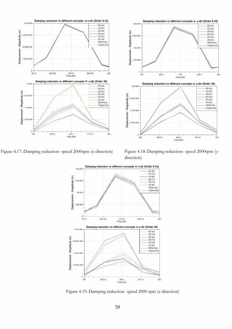
59

Figure 4.17: Damping reduction- speed 2000rpm (x-direction) Figure 4.18: Damping reduction- speed 2000rpm (y-

direction)

Figure 4.19: Damping reduction- speed 2000 rpm (z-direction)

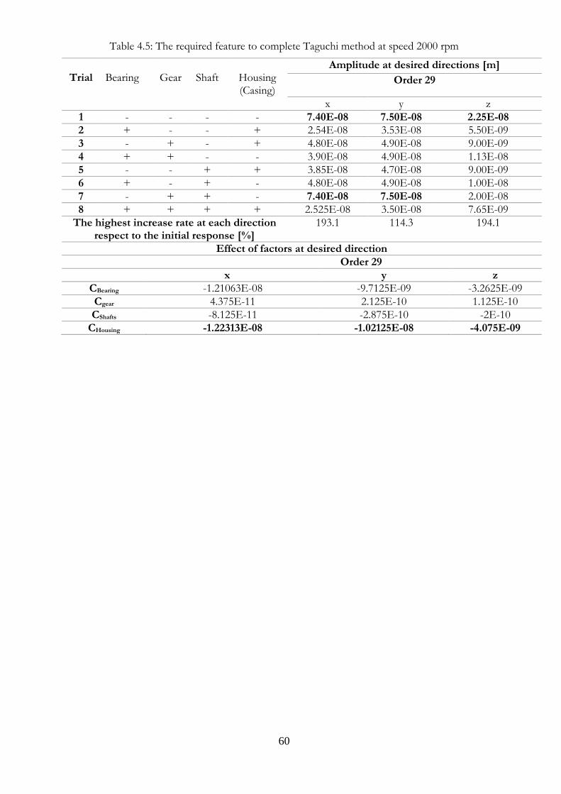
60

Table 4.5: The required feature to complete Taguchi method at speed 2000 rpm

Trial

Bearing

Gear

Shaft

Housing (Casing)

Amplitude at desired directions [m]

Order 29

x y z

1 - - - - 7.40E-08 7.50E-08 2.25E-08

2 + - - + 2.54E-08 3.53E-08 5.50E-09

3 - + - + 4.80E-08 4.90E-08 9.00E-09

4 + + - - 3.90E-08 4.90E-08 1.13E-08

5 - - + + 3.85E-08 4.70E-08 9.00E-09

6 + - + - 4.80E-08 4.90E-08 1.00E-08

7 - + + - 7.40E-08 7.50E-08 2.00E-08

8 + + + + 2.525E-08 3.50E-08 7.65E-09

The highest increase rate at each direction respect to the initial response [%]

193.1 114.3 194.1

Effect of factors at desired direction

Order 29

x y z

CBearing -1.21063E-08 -9.7125E-09 -3.2625E-09

Cgear 4.375E-11 2.125E-10 1.125E-10

CShafts -8.125E-11 -2.875E-10 -2E-10

CHousing -1.22313E-08 -1.02125E-08 -4.075E-09

61

5 Discussion and conclusions

5.1 Discussion The main purpose of this study was to develop an acceptable CAE model in order to simulate the

dynamic behaviour of an electrified powertrain by using AVL Excite. There are two ways to ensure

the developed model is acceptable. First, the responses of the system can be analysed using the

FFT method to observe the excitation frequencies of the system. Second, the results have to be

compared with the experimental measurements to determine their accuracy. In this part, according

to these two criteria, the dynamic behaviour of the model will be interpreted to understand if the

model can accurately represent the dynamic response of the system. The experimental design

analysis using the Taguchi method will also be presented.

5.1.1 Calculated dynamic response error

As shown earlier, the AVL Excite simulations (in almost all cases) differ significantly from the

experimental values. For comparison purposes, the numerical results may not be able to meet the

experimental records with acceptable discrepancies for the following reasons:

First, despite the analogy between the AVL Excite and experimental models, there are some

parameters which have not been accurately determined. In NVH simulations, damping is of key

importance to approach allowable results. In this project, except for the engine mounts, other

elements have been managed with rough damping coefficients. Consequently, the analysis of

results from the AVL Excite model is difficult according to the experimental test. In spite of the

lack of choosing the uncertain values for damping, figures 4.6 to 4.9 can properly show that the

dominant response at each simulation has the same direction as the reference experimental test.

The results, presented in table 4.2, show that the system contains high damping. In order to

investigate the influence of the damping on the results, damping parameters would thus be

reduced. After reducing the damping, it has been realised that the response of the system would

dramatically increase in some cases, for instance for order 8.34 at speed 1500 rpm, whilst it would

be slightly increased for order 29 at this speed. As a result, due to lack of a uniform increment in all

cases, other possible reasons which could influence the response must be taken into account, e.g.

the stiffness of the bearings.

Second, it is assumed that the response around the order bandwidth is completely triangular, see

figure 4.18. This assumption is perhaps the easiest way to integrate the effect of response in the

bandwidth limit and might contain low error. In order to achieve an accurate integration, the

function of response versus frequency must be determined. The plot applies a sort of interpolation

to create the response as a function of frequency. The numbers of recorded responses versus the

frequency is also important. If the number of records is increased, this will give a better resolution

and consequently higher accuracy.

Finally, the error from the experimental recording might be another source of error. There are

some regions where the measurements are quite different from each other, see figure 4.12. In order

to minimize this error, the 4th record was not taken into account. However, there is no guarantee

that other runs are quite acceptable.

62

5.1.2 Dynamic response of the transmission housing

At all examined speeds, the results from the dynamic simulations obviously show the dynamic

behaviour of the system. As discussed previously, the system is excited from two sources. The first

gear mesh generates the fundamental harmonic with order 29 and its multiples while the other gear

mesh provides fundamental order 8.34 and its harmonics. The FFT plots at node 5232902 show a

clear relationship between the gear mesh frequencies and the harmonics, see figures 4.5 and 4.11.

This relationship can also be seen in the Campbell diagram, where it shows the response of the

system at different input shaft speeds.

Other analysis has been carried out to determine how many revolutions would be necessary to

simulate a case. Figure 4.11 illustrates the results from FFT analysis on different cutting signals as

the simulation was performed in 62 cycles at 1500 rpm. The FFT analysis was performed along 36-

40, 47-51 and 58-62 revolutions, respectively. There is no noticeable difference between the results.

As a result, to achieve a steady-state signal, the number of revolutions is not larger than 40 cycles.

This approach is very important and saves a great deal of time and computational resources. Due

to the long runtime of the system, this approach becomes more significant. In this regard, this

analysis can be examined for the other speeds to ensure that the approach gives the same results.

The number of simulations is also very important to determine the dynamic behaviour of the

system. In general, if the number of simulations is low, it is very difficult to show the dynamic

behaviour of the system. This is especially true if a comparison with the experimental tests is

required or desired. For example, by increasing the number of testing speeds, the comparison may

highlight how either the stiffness or the mass of the simulation model can be changed to

accomplish an accurate model. In order to fulfil this objective, the simulation must cover more

testing speeds. In this work, due to lack of sufficient computational resources, the speed rate was

500 rpm, and the growth rate therefore had to be reduced to a lower rate if a more acceptable

approach was desired.

5.1.3 Experimental design analysis

The Taguchi method has been also performed for the AVL Excite model at two speeds, 1500 and

2000 rpm at their fundamental harmonics. The desired objective is to investigate the effect of

damping reduction on the results. The most efficient feature of the design analysis method is to

investigate the AVL Excite model at eight different concepts with the special pattern available in

tables 4.4 and 4.5. The results show that the amplitude will increase after applying damping

reduction. Moreover, the role of housing is of key importance to increase the response level, the

bearings are in the second level of influence and the gears contain the lowest contribution on the

response.

In all modified concepts, the response will be increased. In spite of this; the dependency of the

response on the frequency at each desired direction is different. For instance at 1500 rpm, as

previously seen, the fundamental order 8.34 has been significantly increased after reducing the

damping whilst the response at the fundamental order 29 has been slightly increased. In contrast,

this behaviour is completely reversed at speed 2000 rpm as damping would be reduced. In order to

investigate this dependency as modifying of the model, equations 2.18 and 2.19 must be rewritten

here. These equations refer to particular and general responses of a forced, damped 1DoF.

63

Although, the AVL Excite model has more complexity than the 1DoF model, there is a noticeable

analogy between the characteristics of two models.

x=XP+X0 (2.18)

𝑋𝑝 =𝐹0𝑘

sin(𝜔𝑡−Θ)

√(1−(𝜔

𝜔𝑛)2)2+(

2𝜉𝜔

𝜔𝑛)2

wherein: 𝛩 = 𝑡𝑎𝑛−1(2𝜉𝜔

𝜔𝑛⁄

1−(𝜔

𝜔𝑛)2

) (2.19)

For this system, as expected, reducing the damping results in increasing the amplitude. Also, regarding equation (2.19), for such system, the response is significantly dependent on the excitation frequency.

According to the basic mathematics, equation (2.19) contains some extremum points so that their

positions are determined regarding to the properties of the system, such as mass, damping and

stiffness. Furthermore, the trend of the response, as a function of the external frequency, is

dependent on the position of the excitation frequency relative to the frequencies at extremum

points. This explanation might be used to interpret the trend of the results, not only for the

primary system, without any damping reduction, but also for the system as the damping of the

system is reduced. As a result, for the current model with n-DoFs, the response of the system can

be significantly increased for a fundamental order whilst it can show completely different

behaviour for other fundamental frequency.

5.2 Conclusions This study was conducted to analyse the dynamic behaviour of an electrified power transmission

line using a multibody dynamics simulation tool. The source of excitation was the transmission

error arising from two gear mesh sources. The fundamental orders are 29 and 8.34, respectively,

from the first and second gear mesh configurations. AVL Excite, as a popular simulation tool, was

the CAE tool used to create the simulation model. The experimental results were provided from a

previous project carried out at AVL Vicura. In principle, collecting results from the sensor located

at the housing are the benchmark for validation of the results. In order to validate the results from

other points, it is necessary to mount additional sensors on the housing.

The main purpose of the project was to obtain acceptable records in order to validate the AVL

Excite model with respect to the measurements from the experimental test. There were two criteria

to validate the model. The first criterion is to compare the AVL Excite’ results with the

experimental test. As the other validation tool, the excitation harmonics of the system should be

properly observed in the FFT plots. Although the FFT analysis was completely successful, for

comparison purposes the numerical results showed noticeable discrepancies.

There are some reasons which could cause the discrepancies between the results. First and

foremost, although efforts were made to build the AVL Excite model as similar as possible to the

test-rig, some parameters of the system, such as damping coefficients or bearing stiffness, were not

available. The initial damping parameters established for the model were considered from several

similar projects carried out at AVL Vicura. Furthermore, there were some errors while integrating

the response over the order bandwidth. Other sources of error might come from the experimental

measurements. Overall, three measurements have been fulfilled to measure the response of the

system. However, they are not completely identical.

64

The experimental design analysis gave a deeper knowledge about the behaviour of the damping

effect when two simulations at 1500 and 2000 rpm were run with different damping reduction

concepts. The Taguchi method, as a popular method in vehicle dynamics, indicated that the

housing has the main impact on the amplitude. Although the damping reduction in all cases led to

an increase in the dynamic response, the increase rate for different gear mesh orders was not

identical. This can be explained by the characteristics of the forced damped 1DoF model. Due to

lack of a uniform increment of the response in all cases, other possible reasons must be sought

that might affect the response, e.g. the stiffness of the bearings.

5.3 Future work In order to proceed with this project, to obtain more acceptable results the following

improvements could be made:

In recent years, AVL Excite has been developed rapidly and provides a number of useful dynamic

models required in NVH simulation. AVL Excite has always tried to update the previous models

with more efficient concepts. In order to improve the results, new methods available in the next

version of AVL Excite could therefore be applied.

During this project, the runtime of the simulation was very high. A critical problem is to

investigate how to improve the runtime of the simulation by using updated models, for instance

gear mesh or bearing modelling. How to improve the accuracy of the AVL Excite simulation also

needs to be studied. In this regard, a study to analyse the stiffness of the bearings could be a

priority.

Another criterion to validate the AVL Excite results is the static transmission error. The static

transmission error calculated from the AVL Excite model can be compared with the available

static transmission error given from the LDP program. This was not carried out during this project

due to lack of time.

During the project, the model has been extensively investigated to ensure it would be completely

correct. However, in order to minimize the errors coming from modelling, the model must be fully

investigated in a future study. The discrepancies might be caused by some fundamental problems

in modelling; for example, the brake shafts could be assumed to be flexible. The actual gears used

in the test may also not have exactly the nominal parameter values in the specification due to

tolerances.

Also, if it is possible to perform the experimental test again, a new sensor can be mounted on the

housing. If its location is close to the input shaft, it might be very useful to achieve the results in

order to validate the AVL Excite model according to the experimental measurements.

As long as the characteristics of the system are uncertain, it was difficult to validate of the results

obtained from the program. As a result of the study, the housing and bearings have the highest

effect on the results. The next study could therefore be more concentrated on the housing and

bearings to obtain more acceptable damping parameters. Moreover, the FEM model of the

housing could be investigated. For example, the bolts can be added to the analysis and the model

for gluing two parts of the housing can also be improved.

Attention could be also paid to determining the modal analysis of the system. With this capability,

it might be easier to investigate the dynamic behaviour of the system. Up to the last release of the

65

program, version 2017, it only gives the opportunity to obtain the modal analysis of individual

components. The modal analysis will be released in new versions of AVL Excite.

66

References [1] D. B. Welbourn, Fundamental knowledge of gear noise– A survey. In IMechE Conference on Noise and Vibrations of Engines and Transmissions 1979, Cranfield, 10–12 July 1979, Conference Publications 1979-10, paper C117/79, pp. 9–14. [2] Raul. Tharmakulasingam, Transmission Error in Spur Gears: Static and Dynamic Finite Element Modeling and Design Optimization, School of Engineering and Design, Brunel University, the United Kingdom, October 2009. [3] https://www.researchgate.net/post/What_is_the_mesh_stiffness_of_gears. last visit 2017-08-27 [4] Ivar. Nilsson. Gear whine noise excitation model. Master thesis in mechanical engineering. Chalmers University of technology, Gothenburg, Sweden 2013. [5] Deepak Malviya1, Dr. Pushpendra Kumar Sharma, Transmission Error in Gear, International Journal of Modern Engineering Research (IJMER), Vol. 4| Iss. 1 | Jan. 2014 page 35, ISSN: 2249–6645. [6] http://science.howstuffworks.com/transport/engines-equipment/gear3.htm, last visit 2017-08-29 [7] https://www.cs.cmu.edu/~rapidproto/mechanisms/chpt7.html, last visit 2017-08-29. [8] D. B. Marghitu, Kinematic Chains and Machine Components Design, Academic Press, Waltham, Massachusetts, 2005, pp. 639-646. [9] https://sites.google.com/site/designoftransmissionsystems/Design-of-Gears/design-of-helical-gears last visit 2017-08-29 [10] David. D. Ewins, Modal Testing - Theory, Practice and Application 2e, ISBN: 978-0-86380-218-8. [11] K. Zaveri, M. Phil, Modal Analysis of Large Structures – Multiple Exciter Systems, Brüel and Kjær, November 1984. ISBN 8787355035. [12] L. Meirovitch Analytical Methods in Vibration, the Macmillan Company, ISBN-13: 978-0070413429. [13] Ralph E. Blake, Basic vibration theory, formerly Consultant, Technical Center of Silicon Valley, San Jose, CA. [14] Tobias Larsson, Multibody dynamic simulation in product development, Division of computer aided design, Department of mechanical engineering, Luleå University of technology SE-971 87 Luleå, Sweden, February 2001. [15] O. A. Bauchau. Flexible Multibody Dynamics, volume 176 of Solid Mechanics and Its Applications. Springer Netherlands, 2011. ISBN 978-94-007-0335-3. doi: 10.1007/978-94-007-0335-3. [16] Theory, AVL Excite Power Unit theory manual. Version no. EXTICE v2014. [17] https://www.avl.com/excite, last visit 2017-08-30 [18] Weber, C. and Banaschek, K. "Formaenderung und Profilruecknahme bei gerad- und schraegverzahnten Raedern," Heft 11, F. Vieweg und Sohn, Braunschweig, Germany 1953. [19] Petersen, D., "Auswirkung der Lastverteilung auf die Zahnfusstragfaehigkeit von hoch ueberdeckenden Stirnradpaarungen," Dissertation, Hamburg 1989. [20] R. Craig Jr., A. Kurdila, Fundamentals of Structural Dynamics, 2nd Edition, John Wiley and Sons Inc., Hoboken, New Jersey, 2006. [21] Sebastian Johannes Buckel, Dynamic Substructuring using the Finite Cell Method, Bachelor's thesis for the Bachelor of Science program Engineering Science, Faculty of Civil, Geo and Environmental Engineering, Technische Universität München, November 2014. [22] www.colorado.edu/engineering/CAS/courses.d/IFEM.d/IFEM.Ch10.d/IFEM.Ch10.pdf last visit 2017-08-30 [23] Erwin Kreyszig, Advanced Engineering Mathematics 10th Edition, ISBN-10: 9780470458365. [24] F. C. Nelson, Rotor Dynamics without Equations, Mechanical Engineering Tufts University Medford, MA 02155 USA.

67

[25] W.D. Mark, Analysis of the vibratory excitation of gear systems: basic theory. Journal of the Acoustical Society of America, 1978. [26] F. Kayama, the Dynamics of Parallel Axis Gears in an Automotive Transmission. PhD Thesis, University of Leeds, 2005. [27] W. Tuplin, Gear-tooth stresses at high speed, Proceedings of the Institution of Mechanical Engineers 163 (1950) 162-175. [28] R. Gregory, S. Harris, R. Munro, Dynamic behavior of spur gears, Applied Mechanics Group 178 (8) (1962) 207-221. [29] Y. Wu, J. Wang, Q. Han, Contact finite element method for dynamic meshing characteristics analysis of continuous engaged gear drives, Journal of Mechanical Science and Technology 6 (26) (2012) 1671-1685. [30] www.science.howstuffworks.com/transport/engines-equipment/gear2.htm, last visit 2017-09-09. [31] www.xyobalancer.com/xyo-balancer-blog/gearboxes_gear_mesh_frequency, last visit: 2017-09 09 [32] Samuel Brauer, High speed electric vehicle transmission, Karlstads University, Faculty of Health, science and Technology, spring 2017. [33] http://www.prakashgears.com/helical-gears.htm last visit: 2017-10-01 [34] Carey, W.R.: “Tools for Today’s Engineers”. SAE SP-913. [35] Grove, D.M. and Davis, T.P.: “Engineering Quality and Experimental Design”. Longman, 1992.

TRITA - SCI - GRU 2018:006

www.kth.se