Transactions of the Institute of Measurement and Controldsbaero/library/WindField... · · 2011-07-29Transactions of the Institute of ... 1Department of Mechanical and Aerospace

http://tim.sagepub.com/Measurement and Control

Transactions of the Institute of

http://tim.sagepub.com/content/33/6/718The online version of this article can be found at:

DOI: 10.1177/0142331209342211

February 2010 2011 33: 718 originally published online 24Transactions of the Institute of Measurement and Control

Harish J. Palanthandalam-Madapusi, Anouck Girard and Dennis S. Bernsteinfilter

Wind-field reconstruction from flight data using an unbiased minimum-variance unscented

Published by:

http://www.sagepublications.com

On behalf of:

The Institute of Measurement and Control

can be found at:Transactions of the Institute of Measurement and ControlAdditional services and information for

http://tim.sagepub.com/cgi/alertsEmail Alerts:

http://tim.sagepub.com/subscriptionsSubscriptions:

http://www.sagepub.com/journalsReprints.navReprints:

http://www.sagepub.com/journalsPermissions.navPermissions:

http://tim.sagepub.com/content/33/6/718.refs.htmlCitations:

at UNIVERSITY OF MICHIGAN on July 23, 2011tim.sagepub.comDownloaded from

http://tim.sagepub.com/

http://tim.sagepub.com/content/33/6/718

http://www.sagepublications.com

http://www.instmc.org.uk/

http://tim.sagepub.com/cgi/alerts

http://tim.sagepub.com/subscriptions

http://www.sagepub.com/journalsReprints.nav

http://www.sagepub.com/journalsPermissions.nav

http://tim.sagepub.com/content/33/6/718.refs.html


Wind-field reconstruction fromflight data using an unbiasedminimum-variance unscented filterHarish J. Palanthandalam-Madapusi1,Anouck Girard2 and Dennis S. Bernstein2

1Department of Mechanical and Aerospace Engineering, Syracuse University,Syracuse, NY, USA2Department of Aerospace Engineering, The University of Michigan,Ann Arbor, MI, USA

Although guidance of all aircraft is affected by wind disturbances, micro-unmanned aerialvehicles are especially susceptible. To estimate unknown wind disturbance, we consider twoillustrative scenarios for planar flight. In the first scenario, we assume that measurements of theheading angle are available, while, in the second scenario, we assume that measurements ofthe heading angle are not available. Since the disturbance estimation problem is non-linear, wedevelop an extension of the unscented Kalman filter that provides an estimate of the unknownwind disturbance. Furthermore, we show through simulations that, when the heading angle isnot measured, a kinematic ambiguity is introduced. However, when the initial heading angle isknown and the subsequent heading angle is not measured, this kinematic ambiguity is resolvedand accurate estimates of the wind velocity are obtained.

Key words: input reconstruction, wind estimation, UAV

Notation

x, y Ground coordinates of UAVw Heading angle of UAVx Steering rate

Address for correspondence: Harish J. Palanthandalam-Madapusi, Department of Mechanicaland Aerospace Engineering, 149 Link Hall, Syracuse University, Syracuse, NY 13244, USA.E-mail: [email protected] 2–9 appear in colour online: http://tim.sagepub.com

Transactions of the Institute of Measurement and Control 33, 6 (2011) pp. 718–733

� 2010 The Institute of Measurement and Control 10.1177/0142331209342211



VAC/W Airspeed of UAVVW/E, u Magnitude and direction of wind velocity, respectivelyVAC/E, � Magnitude and direction of aircraft velocity, respectivelyVW/E,x, VW/E,y x and y component of wind velocity, respectivelyxk State vector at time step kyk Output vector at time step kuk Known input vector at time step kwk, vk Process noise and sensor noise at time step k, respectivelyAk, Bk, Ck, Gk State-space matrices at time step kx0;R k Mean and covariance of the initial state vector, respectivelyQk, Rk Process noise covariance and sensor noise covariance at time step k,

respectivelyJ(xk) Cost functionq(p\q) Conditional probability density function of p given qxk State estimaten Order of a system (dimension of the state vector)xknk�1 State estimate after forecast step at time step kyknk�1 Estimate of output after forecast step at time step kPxx

knk�1;Pyyknk�1;P

xyknk�1 State error covariance, output error covariance, and cross error

covariance after forecast step at time step kPxx

knk Error covariance at time step kKk Kalman filter gain at time step kek Unknown input vector at time step kHk Unknown-input matrix at time step kPk, Vk Intermediate quantities in the computation of unbiased minimum-

variance filter gainLk Unbiased minimum-variance filter gain at time step kek Estimate of the unknown input at time step kfk, hk Functions representing the process and observation models,

respectivelyx a

k Augmented state vector at time step kna Dimension of the augmented state vectorp xxa

k Augmented error covariance at time step k�k Sigma-point matrix at time step kcoli (A) ith column of matrix A(A)1/2 Cholesky square root of matrix A�, a, �, � Parameters of unscented Kalman filter�i Weights1p�q p by q matrix of ones

1. Introduction

Small and micro air vehicles are increasingly being used to improve situationalawareness by conducting surveillance, patrolling, and convoy protection (Office ofthen Secretary of Defense, 2005). These vehicles provide imagery reconnaissance

Palanthandalam-Madapusi et al. 719



capability out to five to ten miles at the company/platoon/squad level. Due to theirsmall size, these aircraft have limited payload capacity and usually carry fixedcameras (which require accurate pointing, therefore accurate knowledge of heading)and commercial off-the-shelf autopilots (which often have poor heading-measurementaccuracy) (Gross et al., 2006).

Although guidance of all aircraft is affected by the atmospheric motion relative tothe Earth, that is, wind, micro-unmanned aerial vehicles (micro-UAVs) are especiallysusceptible. Localized wind-field estimation, especially winds at low velocity, isdifficult. Consequently, alternative means must be used to assess the effects of wind.Efforts in this direction include wind estimation (Osborne and Rysdyk, 2005;Rodriguez and Taylor, 2007), and techniques for path planning in wind, for example(McGee et al., 2006; Ceccarelli et al., 2007), which assume constant known wind fields,and (Rysdyk, 2006; Thomasson, 1998), which make use of gimballed cameras.

In the present paper we develop a technique for using available measurements toestimate the local wind-field velocity. To do this, we use state-estimation techniquesthat have the ability to reconstruct exogenous disturbance signals that are not directlymeasured.

In the case of linear systems, early work on reconstructing exogenous signalsincludes input reconstruction through system inversion (Sain and Massey, 1969;Moylan, 1977), while methods using optimal filters are developed in (Glover, 1969;Corless and Tu, 1998; Hou and Patton, 1998; Xiong and Saif, 2003). More recently, atechnique for reconstructing unknown exogenous disturbances has been developed in(Gillijns and De Moor, 2005; Palanthandalam-Madapusi et al., 2006; Palanthandalam-Madapusi and Benrstein, 2007) as an extension of unbiased minimum-variancefiltering (Kitanidis, 1987).

In this paper, we extend the techniques in (Palanthandalam-Madapusi andBenrstein, 2007) for estimating unknown external disturbances for non-linear systems.This technique is based on the unscented Kalman filter (UKF) (Julier et al., 2000; Julierand Uhlmann, 2004) for state estimation for non-linear systems, which is an exampleof sigma-point Kalman filters (SPKF) (van der Merwe et al., 2004). Recent work(Julier et al., 2000; van der Merwe et al., 2004) illustrates the improved performance ofSPKFs compared to the extended Kalman filter (EKF), which is prone to numericalproblems such as initialization sensitivity, bias (divergence), and instability forstrongly non-linear systems.

The nature of the disturbance estimation (input reconstruction) problem dependson the type of measurements available. In the present paper we consider twoillustrative scenarios for planar flight. In the first scenario, we assume thatmeasurements of the heading angle are available. In this case, the estimation problemis linear, and the techniques of (Gillijns and De Moor, 2005; Palanthandalam-Madapusi et al., 2006; Palanthandalam-Madapusi and Benrstein, 2007) are applicable.In the second scenario, we assume that measurements of the heading angle are notavailable. In this case, the disturbance estimation problem is non-linear, and we

720 Wind-field reconstruction from flight data



therefore develop an extension of the unscented Kalman filter that provides anestimate of the unknown disturbance.

After describing the basic setting in Section 2, the two scenarios described above aredeveloped in Sections 3 and 4. For each scenario, we consider flight involving straight-line and circular motion in the presence of a wind field that varies as a triangularwaveform in both of its components. In the case of unknown heading angle, we showthat wind field estimation requires knowledge of the initial heading angle in order toremove a kinematic ambiguity.

2. Wind-field estimation

Consider the planar flight equations

_x ¼ VAC=W cos þ VW=E cos �, ð2:1Þ

_y ¼ VAC=W sin þ VW=E sin�, ð2:2Þ

_ ¼ !, ð2:3Þ

where x and y are the ground coordinates of the vehicle, VAC/W is the airspeed of thevehicle, is the heading angle, ! is the steering angle rate, VW/E is the horizontalwind speed, and � is the angle of the direction of the horizontal component of windas measured from the ı axis. The magnitude and direction of velocity of the vehiclewith respect to the Earth are VAC=E¼

4ffiffiffiffiffiffiffiffiffiffiffiffiffiffiffi_x2 þ _y2

pand �¼

4tan�1 ð_y=_xÞ, respectively; note

that VAC/E¼VAC/WþVW/E. The relationship between the various components ofvelocities is illustrated in Figure 1. Throughout this paper, we assume thatmeasurements of x and y are available from GPS, and that measurements of VAC/W

are available from an airspeed sensor. For simplicity, we assume that VAC/W is alignedwith the heading angle as depicted in Figure 1. We consider the problem ofestimating the unknown wind speed VW/E and angle � of the wind.

j

ˆ

VAC/W

VAC/E

VW/E

ψθ

φ

i

Figure 1 Schematic of relationship between components ofvelocities in an Earth-fixed frame and the body-fixed frame




3. Measured heading angle

We first consider the case in which the heading angle is measured. In this case, weuse (2.1) and (2.2) to estimate VW/E and �. By defining

VW=E,x¼4

VW=E cos�, ð3:1Þ

VW=E,y¼4

VW=E sin�, ð3:2Þ

it follows that (2.1), (2.2) are linear in the unknowns VW/E,x and VW/E,y. Once estimatesof VW/E,x and VW/E,y are obtained, the wind speed VW/E and angle � can be obtainedusing the relationships

VW=E ¼

ffiffiffiffiffiffiffiffiffiffiffiffiffiffiffiffiffiffiffiffiffiffiffiffiffiffiffiffiffiffiffiffiffiV2

W=E,x þ V2W=E,y

q, ð3:3Þ

� ¼ tan�1 VW=E,y

VW=E,x

� �: ð3:4Þ

Thus the problem is stated as follows.

Problem 1. Equations:

_x ¼ VAC=W cos þ VW=E,x, ð3:5Þ

_y ¼ VAC=W sin þ VW=E,y: ð3:6Þ

Available measurements: x, y, VAC/W, and .Unknowns: VW/E,x and VW/E,y.

Since Problem 1 is linear in the states and linear in the unknowns VW/E,x andVW/E,y, we can use the unbiased minimum-variance filter (Palanthandalam-Madapusi and Benrstein, 2007) for linear systems to estimate the states and theunknown inputs. We briefly review the Kalman filter and the unbiased minimum-variance filter.

3.1 Kalman filter

For the linear stochastic discrete-time dynamic system

xk ¼ Ak�1xk�1 þ Bk�1uk�1 þ Gk�1wk�1, ð3:7Þ

yk ¼ Ckxk þ vk, ð3:8Þ

where Ak�12Rn�n, Bk�12R

n�p, Gk�12Rn�q, and Ck2R

m�n are known matrices, thestate-estimation problem can be described as follows. Assume that, for all k� 1,




the known data are the measurements yk2Rm, the inputs uk�12R

p, and the statistical

properties of x0, wk�1 and vk. The initial state vector x02Rn is assumed to be Gaussian

with mean x0 and error covariance Pxx0 ,E½ðx0 � x0Þðx0 � x0Þ

T�. The process noise

wk�12Rq, which represents unknown input disturbances, and the measurement noise

vk2Rm, concerning inaccuracies in the measurements, are assumed white, Gaussian,

zero mean, and mutually independent with known covariance matrices Qk�1 and Rk,respectively. Next, define the cost function

JðxkÞ¼4ðxkjðy1, . . . , ykÞÞ, ð3:9Þ

which is the conditional probability density function of the state vector xk2Rn given

the past and present measured data y1, . . . , yk. Under the stated assumptions, the

maximization of (3.9) is the state-estimation problem, while the maximizer xk of J is the

optimal state estimate.The optimal state estimate xk is given by the Kalman filter (Kalman, 1960), whose

forecast step is given by

xkjk�1 ¼ Ak�1xk�1 þ Bk�1uk�1, ð3:10Þ

Pxxkjk�1 ¼ Ak�1Pxx

k�1ATk�1 þ Gk�1Qk�1GT

k�1, ð3:11Þ

ykjk�1 ¼ Ckxkjk�1, ð3:12Þ

Pyykjk�1 ¼ CkPxx

kjk�1CTk þ Rk, ð3:13Þ

Pxykjk�1 ¼ Pxx

kjk�1CTk , ð3:14Þ

where Pxxkjk�1¼

4E½ðxk � xkjk�1Þðxk � xkjk�1Þ

T�, P

yykjk�1¼

4E½ð yk � ykjk�1Þð yk � ykjk�1Þ

T�, and

Pxykjk�1¼

4E½ðxk � xkjk�1Þð yk � ykjk�1Þ

T�, and whose data-assimilation step is given by

Kk ¼ Pxykjk�1ðP

yykjk�1Þ

�1, ð3:15Þ

xk ¼ xkjk�1 þ Kkðyk � ykjk�1Þ, ð3:16Þ

Pxxk ¼ Pxx

kjk�1 � KkPyykjk�1KT

k , ð3:17Þ

where Pxxk ¼4

E½ðxk � xkÞðxk � xkÞT� is the error-covariance matrix and Kk is the Kalman

gain matrix. The notation zkjk�1 indicates an estimate of zk at time k based on

information available up to and including time k� 1. Likewise, zk indicates an

estimate of z at time k using information available up to and including time k. Modelinformation is used during the forecast step, while measurement data are injected into

the estimates during the data-assimilation step, specifically, (3.16).




3.2 Unbiased minimum-variance filter

Consider the system

xk ¼ Ak�1xk�1 þ Bk�1uk�1 þHk�1ek�1 þ Gk�1wk�1, ð3:18Þ

yk ¼ Ckxk þ vk, ð3:19Þ

where xk, yk, uk�1, Ak�1, Bk�1, Gk�1 and Ck are defined as in Section 3.1, while ek�12Rl

represents the unknown input and Hk�12Rn�l is the input matrix. We assume that

Ak�1, Bk�1, Ck, Dk, and Hk�1 are known, while ek�1 is unknown.Owing to the presence of the unknown non-zero-mean term Hk�1ek�1, the Kalman

filter estimate in Section 3.1 is biased in general. The optimal unbiased state estimate

xk is given by the Unbiased Minimum-Variance (UMV) filter (Palanthandalam-

Madapusi and Benrstein, 2007), whose forecast step is given by (3.10)–(3.14), andwhose data-assimilation step is given by

Vk¼4

CkHk�1, ð3:20Þ

�k¼4ðVT

k ðPyykjk�1Þ

�1VkÞ�1VT

k ðPyykjk�1Þ

�1, ð3:21Þ

Lk ¼ Hk�1�k þ Pxykjk�1ðP

yykjk�1Þ

�1ðI � Vk�kÞ, ð3:22Þ

xk ¼ xkjk�1 þ Lkðyk � ykjk�1Þ, ð3:23Þ

Pxxk ¼ Pxx

kjk�1 � LkPyykjk�1LT

k , ð3:24Þ

where Lk is the UMV filter gain matrix. Finally, the estimate of the unknown signal ek�1

is given by

ek�1 ¼ Hyk�1Lkð yk � Ckxkjk�1 �DkukÞ: ð3:25Þ

3.3 Results: wind estimation with measured heading angle

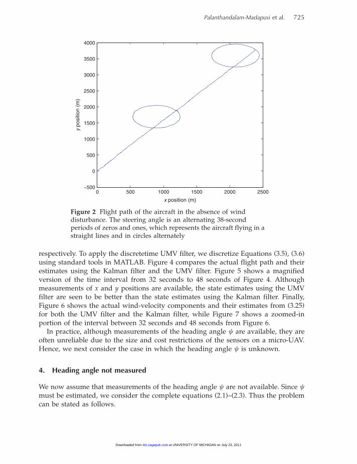
The steering angle is chosen to be alternating 38-second periods of zeros and ones,which represents the aircraft flying alternately in a straight line and in circles. The

wind-velocity component profiles are chosen to be triangular waveforms. Figure 2

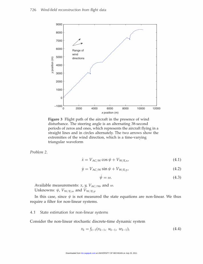
shows the flight path in the absence of wind disturbance, while Figure 3 shows the

flight path in the presence of the wind disturbance.Since Problem 1 is linear in the unknown wind-velocity components, we apply the

UMV filter (3.20)–(3.24) and (3.25) to estimate the states and unknown inputs,




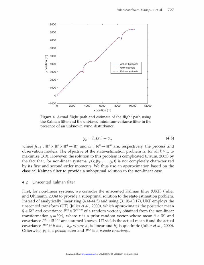
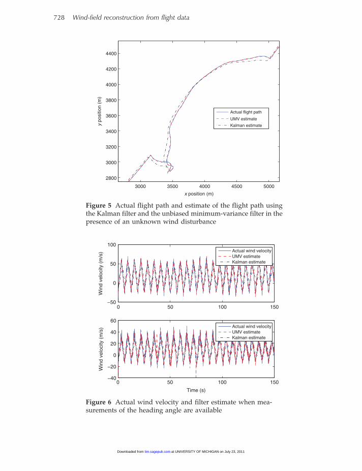
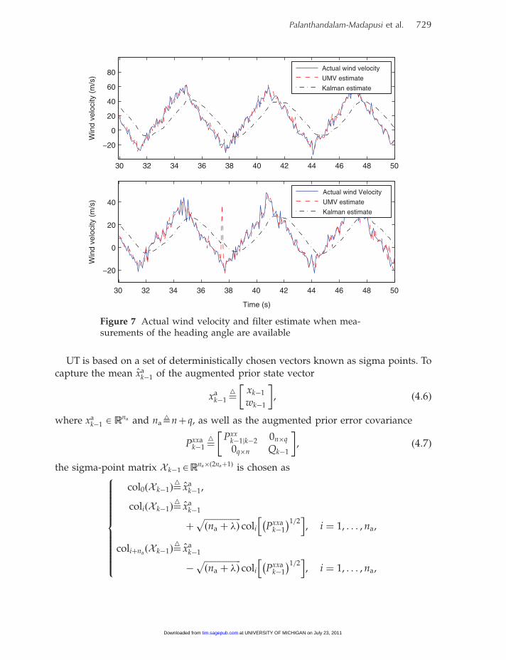
respectively. To apply the discretetime UMV filter, we discretize Equations (3.5), (3.6)using standard tools in MATLAB. Figure 4 compares the actual flight path and theirestimates using the Kalman filter and the UMV filter. Figure 5 shows a magnifiedversion of the time interval from 32 seconds to 48 seconds of Figure 4. Althoughmeasurements of x and y positions are available, the state estimates using the UMVfilter are seen to be better than the state estimates using the Kalman filter. Finally,Figure 6 shows the actual wind-velocity components and their estimates from (3.25)for both the UMV filter and the Kalman filter, while Figure 7 shows a zoomed-inportion of the interval between 32 seconds and 48 seconds from Figure 6.

In practice, although measurements of the heading angle are available, they areoften unreliable due to the size and cost restrictions of the sensors on a micro-UAV.Hence, we next consider the case in which the heading angle is unknown.

4. Heading angle not measured

We now assume that measurements of the heading angle are not available. Since must be estimated, we consider the complete equations (2.1)–(2.3). Thus the problemcan be stated as follows.

0 500 1000 1500 2000 2500−500

0

500

1000

1500

2000

2500

3000

3500

4000

y po

sitio

n (m

)

x position (m)

Figure 2 Flight path of the aircraft in the absence of winddisturbance. The steering angle is an alternating 38-secondperiods of zeros and ones, which represents the aircraft flying in astraight lines and in circles alternately




Problem 2.

_x ¼ VAC=W cos þ VW=E,x, ð4:1Þ

_y ¼ VAC=W sin þ VW=E,y, ð4:2Þ

_ ¼ !: ð4:3Þ

Available measurements: x, y, VAC/W, and !.Unknowns: , VW/E,x, and VW/E,y.

In this case, since is not measured the state equations are non-linear. We thusrequire a filter for non-linear systems.

4.1 State estimation for non-linear systems

Consider the non-linear stochastic discrete-time dynamic system

xk ¼ fk�1 xk�1, uk�1, wk�1ð Þ, ð4:4Þ

0 2000 4000 6000 8000 10000 12000−1000

0

1000

2000

3000

4000

5000

6000

7000

8000

9000

Range ofwinddirections

y po

sitio

n (m

)

x position (m)

Figure 3 Flight path of the aircraft in the presence of winddisturbance. The steering angle is an alternating 38-secondperiods of zeros and ones, which represents the aircraft flying in astraight lines and in circles alternately. The two arrows show theextremities of the wind direction, which is a time-varyingtriangular waveform




yk ¼ hk xkð Þ þ vk, ð4:5Þ

where fk�1 : Rn�R

p�R

q!R

n and hk : Rn!R

m are, respectively, the process andobservation models. The objective of the state-estimation problem is, for all k� 1, tomaximize (3.9). However, the solution to this problem is complicated (Daum, 2005) bythe fact that, for non-linear systems, (xkj(y1, . . . , yk)) is not completely characterizedby its first and second-order moments. We thus use an approximation based on theclassical Kalman filter to provide a suboptimal solution to the non-linear case.

4.2 Unscented Kalman filter

First, for non-linear systems, we consider the unscented Kalman filter (UKF) (Julierand Uhlmann, 2004) to provide a suboptimal solution to the state-estimation problem.Instead of analytically linearizing (4.4)–(4.5) and using (3.10)–(3.17), UKF employs theunscented transform (UT) (Julier et al., 2000), which approximates the posterior meany 2 R

m and covariance Pyy2R

m�m of a random vector y obtained from the non-lineartransformation y¼ h(x), where x is a prior random vector whose mean x 2 R

n andcovariance Pxx

2Rn�n are assumed known. UT yields the actual mean y and the actual

covariance Pyy if h¼ h1þ h2, where h1 is linear and h2 is quadratic (Julier et al., 2000).Otherwise, yk is a pseudo mean and Pyy is a pseudo covariance.

0 2000 4000 6000 8000 10000 12000−1000

0

1000

2000

3000

4000

5000

6000

7000

8000

9000

Actual flight path

UMV estimate

Kalman estimatey po

sitio

n (m

)

x position (m)

Figure 4 Actual flight path and estimate of the flight path usingthe Kalman filter and the unbiased minimum-variance filter in thepresence of an unknown wind disturbance




3000 3500 4000 4500 5000

2800

3000

3200

3400

3600

3800

4000

4200

4400

Actual flight path

UMV estimate

Kalman estimatey po

sitio

n (m

)

x position (m)

Figure 5 Actual flight path and estimate of the flight path usingthe Kalman filter and the unbiased minimum-variance filter in thepresence of an unknown wind disturbance

0 50 100 150−50

0

50

100

Win

d ve

loci

ty (

m/s

) Actual wind velocityUMV estimateKalman estimate

0 50 100 150−40

−20

0

20

40

60

Time (s)

Win

d ve

loci

ty (

m/s

) Actual wind velocityUMV estimateKalman estimate

Figure 6 Actual wind velocity and filter estimate when mea-surements of the heading angle are available




UT is based on a set of deterministically chosen vectors known as sigma points. To

capture the mean xak�1 of the augmented prior state vector

xak�1¼

4 xk�1

wk�1

� �, ð4:6Þ

where xak�1 2 R

na and naXnþ q, as well as the augmented prior error covariance

Pxxak�1¼

4 Pxxk�1jk�2 0n�q

0q�n Qk�1

� �, ð4:7Þ

the sigma-point matrix X k�12Rna�ð2naþ1Þ is chosen as

col0ðX k�1Þ¼4

xak�1,

coliðX k�1Þ¼4

xak�1

þffiffiffiffiffiffiffiffiffiffiffiffiffiffiffiffiffiðna þ �Þ

pcoli Pxxa

k�1

� �1=2h i

, i ¼ 1, . . . , na,

coliþnaðX k�1Þ¼

4xa

k�1

�ffiffiffiffiffiffiffiffiffiffiffiffiffiffiffiffiffiðna þ �Þ

pcoli Pxxa

k�1

� �1=2h i

, i ¼ 1, . . . , na,

8>>>>>>>>>><>>>>>>>>>>:

30 32 34 36 38 40 42 44 46 48 50

−20

0

20

40

60

80

Win

d ve

loci

ty (

m/s

)

Actual wind velocity

UMV estimate

Kalman estimate

30 32 34 36 38 40 42 44 46 48 50

−20

0

20

40

Time (s)

Win

d ve

loci

ty (

m/s

)

Actual wind Velocity

UMV estimate

Kalman estimate

Figure 7 Actual wind velocity and filter estimate when mea-surements of the heading angle are available




with weights

�ðmÞ0 ¼4 �

na þ �,

�ðcÞ0 ¼4 �

na þ �þ 1� 2 þ �,

�ðmÞi ¼4�ðcÞi ¼

4�ðmÞiþna¼4�ðcÞiþna

,1

2ðna þ �Þ, i ¼ 1, . . . , na,

8>>>>>><>>>>>>:

where coli[(�)1/2] is the ith column of the Cholesky square root, 05� 1, �� 0, �� 0,

and �X2(�þ na)� na. We set ¼ 1 and �¼ 0 (Haykin, 2001) such that �¼ 0 (Julier and

Uhlmann, 2004) and set �¼ 2 (Haykin, 2001). Alternative schemes for choosing sigma

points are given in (Julier and Uhlmann, 2004).The UKF forecast equations are given by

X k�1 ¼ xak�1 xa

k�111�naþ

ffiffiffiffiffiffiffiffiffiffiffiffiffiffiffiffiffiðna þ �Þ

pPxxa

k�1

� �1=2xa

k�111�na�

ffiffiffiffiffiffiffiffiffiffiffiffiffiffiffiffiffiðna þ �Þ

pPxxa

k�1

� �1=2h i

,

ð4:8Þ

coliðXxkjk�1Þ ¼ fk�1ðcoliðX

xk�1Þ, uk�1, coliðX

wk�1ÞÞ, i ¼ 0, . . . , 2na, ð4:9Þ

xkjk�1 ¼X2na

i¼0

�ðmÞi coliðXxkjk�1Þ, ð4:10Þ

Pxxkjk�1 ¼

X2na

i¼0

�ðcÞi ½coliðXxkjk�1Þ � xkjk�1�½coliðX

xkjk�1Þ � xkjk�1�

T, ð4:11Þ

coliðYkjk�1Þ ¼ hkðcoliðXxkjk�1ÞÞ, i ¼ 0, . . . , 2na, ð4:12Þ

ykjk�1 ¼X2na

i¼0

�ðmÞi coliðYkjk�1Þ, ð4:13Þ

Pyykjk�1 ¼

X2na

i¼0

�ðcÞi ½coliðYkjk�1Þ � ykjk�1�½coliðYkjk�1Þ � ykjk�1�Tþ Rk, ð4:14Þ

Pxykjk�1 ¼

X2na

i¼0

�ðcÞi ½coliðXxkjk�1Þ � xkjk�1�½coliðYkjk�1Þ � ykjk�1�

T, ð4:15Þ

where

Xxk�1

Xwk�1

� �¼4X k�1;X

xk�1 2 R

n�ð2naþ1Þ; and Xwk�1 2 R

q�ð2naþ1Þ:

The UKF data-assimilation equations are given by (3.15)–(3.17).




4.3 Unbiased minimum-variance unscented filter

Next, for non-linear systems with unknown inputs, we consider an extension of the

UKF along the lines of the linear UMV filter. Thus, to obtain the pseudo mean and the

pseudo error covariances we use the unscented transform, and to estimate the states

and unknown inputs, we use the expressions derived for the UMV filter. Thus, the

forecast equations for the unbiased minimum-variance unscented (UMVU) filter aregiven by (4.8)–(4.15). The data-assimilation equations for the UMVU filter are given by

(3.20)–(3.24).

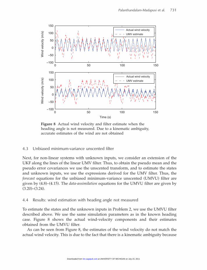
4.4 Results: wind estimation with heading angle not measured

To estimate the states and the unknown inputs in Problem 2, we use the UMVU filter

described above. We use the same simulation parameters as in the known heading

case. Figure 8 shows the actual wind-velocity components and their estimates

obtained from the UMVU filter.As can be seen from Figure 8, the estimates of the wind velocity do not match the

actual wind velocity. This is due to the fact that there is a kinematic ambiguity because

0 50 100 150−100

−50

0

50

100

150

Win

d ve

loci

ty (

m/s

) Actual wind velocity

UMV estimate

0 50 100 150−100

−50

0

50

100

150

Time (s)

Win

d ve

loci

ty (

m/s


UMV estimate

Figure 8 Actual wind velocity and filter estimate when theheading angle is not measured. Due to a kinematic ambiguity,accurate estimates of the wind are not obtained




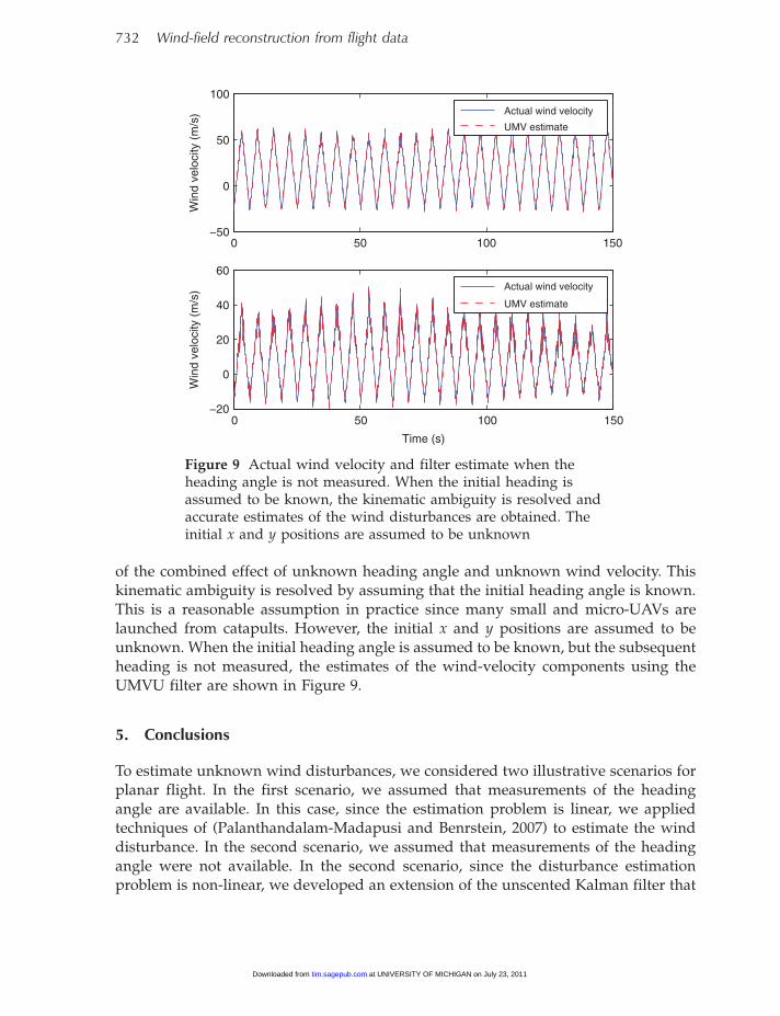
of the combined effect of unknown heading angle and unknown wind velocity. Thiskinematic ambiguity is resolved by assuming that the initial heading angle is known.This is a reasonable assumption in practice since many small and micro-UAVs arelaunched from catapults. However, the initial x and y positions are assumed to beunknown. When the initial heading angle is assumed to be known, but the subsequentheading is not measured, the estimates of the wind-velocity components using theUMVU filter are shown in Figure 9.

5. Conclusions

To estimate unknown wind disturbances, we considered two illustrative scenarios forplanar flight. In the first scenario, we assumed that measurements of the headingangle are available. In this case, since the estimation problem is linear, we appliedtechniques of (Palanthandalam-Madapusi and Benrstein, 2007) to estimate the winddisturbance. In the second scenario, we assumed that measurements of the headingangle were not available. In the second scenario, since the disturbance estimationproblem is non-linear, we developed an extension of the unscented Kalman filter that

0 50 100 150−50

0

50

100

Win

d ve

loci

ty (

m/s


UMV estimate

0 50 100 150−20

0

20

40

60

Time (s)

Win

d ve

loci

ty (

m/s


UMV estimate

Figure 9 Actual wind velocity and filter estimate when theheading angle is not measured. When the initial heading isassumed to be known, the kinematic ambiguity is resolved andaccurate estimates of the wind disturbances are obtained. Theinitial x and y positions are assumed to be unknown




provided an estimate of the unknown wind disturbance. When the heading angle isnot measured, a kinematic ambiguity was introduced. However, when the initialheading angle was known and the subsequent heading angle was not measured, thiskinematic ambiguity was resolved and accurate estimates of the wind disturbancewere obtained.

ReferencesCeccarelli, N., et al. 2007: Micro AUV Path

Planning for Reconnaissance in Wind.Proceedings of the 2007 American ControlConference, New York, NY, July 11-13, 6310–16.

Corless, M. and Tu, J. 1998: State and inputestimation for a class of uncertain systems.Automatica 34(6): 757–64.

Daum, F.E. 2005: Nonlinear filters: Beyond theKalman filter. IEEE Aerospace and ElectronicsSystems Magazine 20(8): 57–69.

Gillijns, S. and De Moor, B. 2005: Unbiasedminimum-variance input and state estima-tion for linear discrete-time stochastic sys-tems. Internal Report ESAT-SISTA/TR 05-228.Katholieke Universiteit Leuven, Leuven.

Glover, J.D. 1969: The linear estimation ofcompletely unknown systems. IEEETransactions on Automatic Control 14, 766–7.

Gross, D., et al. 2006: Cooperative Operationsin Urban TERrain (COUNTER). SPIE Defenseand Security Symposium. Orlando, FL, April.

Haykin S. editor, 2001: Kalman Filtering andNeural Networks. Wiley Publishing,New York.

Hou, M. and Patton, R.J. 1998: Input observa-bility and input reconstruction. Automatica34(6): 789–94.

Julier, S.J. and Uhlmann, J.K. 2004: Unscentedfiltering and nonlinear estimation.Proceedings of the IEEE 92, 401–22.

Julier, S.J., et al. 2000: A new method for thenonlinear transformation of means and covar-iances in filters and estimators. IEEETransactions on Automatic Control 45(3): 477–82.

Kalman, R.E. 1960: A new approach to linearfiltering and prediction problems.Transactions of the ASME – Journal of BasicEngineering 82, 35–45.

Kitanidis, P.K. 1987: Unbiased Minimum-vari-ance Linear State Estimation. Automatica23(6): 775–78.

McGee, T.G., et al. 2006: Optimal Path Planningin a Constant Wind with a Bounded TurningRate. AIAA Conference on Guidance, Navigation,and Control, Keystone, CO.

Moylan, P.J. 1977: Stable inversion of linearsystems. IEEE Transactions on AutomaticControl 22, 74–78.

Office of the Secretary of Defense. 2005:Unmanned Aircraft Systems Roadmap, 2005–2030.

Osborne, J. and Rysdyk, R. 2005: WaypointGuidance for Small UAVs in Wind. AIAAInfotech@Aerospace. Arlington, VA.

Palanthandalam-Madapusi, H.J. andBenrstein, D.S. 2007: Unbiased minimum-variance filtering for input reconstruction.Proceedings of the 2007 American ControlConference, New York, NY, July.

Palanthandalam-Madapusi, H., et al. 2006:System identification for nonlinear modelupdating. Proceedings of the 2006 AmericanControl Conference, Minneapolis, MN, June.

Rodriguez, A. and Taylor, C. 2007: WindEstimation Using an Optical Flow Sensoron a Miniature Air Vehicle. AIAA Conferenceon Guidance, Navigation and Control, HiltonHead, SC, August.

Rysdyk, R. 2006: Unmanned Aerial VehiclePath Following for Target Observation inWind. Journal of Guidance, Control, andDynamics 29(5): 1092–100.

Sain, M.K. and Massey, J.L. 1969: Invertibilityof linear time-invariant dynamical systems.IEEE Transactions on Automatic Control 14(2):141–9.

Thomasson, P.G. 1998: Guidance of a Roll-Only Camera for Ground Observation inWind. Journal of Guidance, Control, andDynamics 21(1): 39–44.

van der Merwe, R., et al. 2004: Sigma-pointKalman filters for nonlinear estimation andsensor-fusion – applications to integratednavigation. Proceedings of the AIAAGuidance, Navigation & Control Conference.Providence, RI.

Xiong, Y. and Saif, M. 2003: Unknown distur-bance inputs estimation based on a statefunctional observer design. Automatica 39,1389–98.




Transactions of the Institute of Measurement and Controldsbaero/library/WindField... · · 2011-07-29Transactions of the Institute of ... 1Department of Mechanical and Aerospace

Documents