Traffic Impacts on Fine Particulate Matter Air Pollution at the Urban Project Scale: A Quantitative Assessment

Journal of Environmental Protection, 2013, 4, 49-62 Published Online December 2013 (http://www.scirp.org/journal/jep) http://dx.doi.org/10.4236/jep.2013.412A1006

Open Access JEP

Traffic Impacts on Fine Particulate Matter Air Pollution at the Urban Project Scale: A Quantitative Assessment

Chidsanuphong Chart-asa, Kenneth G. Sexton, Jacqueline MacDonald Gibson

University of North Carolina at Chapel Hill, Chapel Hill, USA. Email: [email protected], [email protected], [email protected] Received September 9th, 2013; revised October 13th, 2013; accepted November 11th, 2013 Copyright © 2013 Chidsanuphong Chart-asa et al. This is an open access article distributed under the Creative Commons Attribution License, which permits unrestricted use, distribution, and reproduction in any medium, provided the original work is properly cited. In accordance of the Creative Commons Attribution License all Copyrights © 2013 are reserved for SCIRP and the owner of the intellectual property Chidsanuphong Chart-asa et al. All Copyright © 2013 are guarded by law and by SCIRP as a guardian.

ABSTRACT

Formal health impact assessment (HIA), currently underused in the United States, is a relatively new process for assist-ing decision-makers in non-health sectors by estimating the expected public health impacts of policy and planning deci-sions. In this paper we quantify the expected air quality impacts of increased traffic due to a proposed new university campus extension in Chapel Hill, North Carolina. In so doing, we build the evidence base for quantitative HIA in the United States and develop an improved approach for forecasting traffic effects on exposure to ambient fine particulate matter (PM2.5) in air. Very few previous US HIAs have quantified health impacts and instead have relied on stake-holder intuition to decide whether effects will be positive, negative, or neutral. Our method uses an air dispersion model known as CAL3QHCR to predict changes in exposure to airborne, traffic-related PM2.5 that could occur due to the proposed new campus development. We employ CAL3QHCR in a new way to better represent variability in road grade, vehicle driving patterns (speed, acceleration, deceleration, and idling), and meteorology. In a comparison of model pre-dictions to measured PM2.5 concentrations, we found that the model estimated PM2.5 dispersion to within a factor of two for 75% of data points, which is within the typical benchmark used for model performance evaluation. Applying the model to present-day conditions in the study area, we found that current traffic contributes a relatively small amount to ambient PM2.5 concentrations: about 0.14 µg/m3 in the most exposed neighborhood—relatively low in comparison to the current US National Ambient Air Quality Standard of 12 µg/m3. Notably, even though the new campus is ex-pected to bring an additional 40,000 daily trips to the study community by the year 2025, vehicle-related PM2.5 emis-sions are expected to decrease compared to current conditions due to anticipated improvements in vehicle technologies and cleaner fuels. Keywords: PM2.5; Traffic; Health Impact Assessment

1. Introduction

The World Health Organization and other public health advocates have long stressed the need for formal health impact assessment (HIA) to inform decision-making in sectors outside the health-care industry [1-3]. The ration-ale is that chronic diseases that pose major health bur-dens in the post-industrial world are driven largely by policy, program, and planning decisions in transportation, agriculture, urban planning, and other sectors that ordi-narily do not include population health as an objective in their decision processes. Commonly cited examples in-clude the effects of government agricultural subsidies on the availability of healthy foods and the effects of trans-

portation plans on population exposure to noise and air pollution. HIA is intended to encourage decision-makers in these and other sectors to make choices that minimize negative and maximize positive impacts on public health, within budgetary and other constraints. The intent of HIA is to prevent the chronic, noninfectious diseases—including heart disease, stroke, and diabetes—that have replaced infectious diseases as the leading health con-cerns in post-industrialized nations [4]. Health practitio-ners have long recognized that exposures to risk factors for these chronic diseases are driven by a wide range of policy, planning, and program decisions in multiple sec-tors and that prevention through better-informed deci-

Traffic Impacts on Fine Particulate Matter Air Pollution at the Urban Project Scale: A Quantitative Assessment 50

sion-making in all sectors is likely to be less costly than treating the symptoms [2].

While the practice of HIA is well established in the European Union and some other nations, in the United States HIA practice is relatively new [2,5,6]. The first U.S. HIA, which evaluated the health impacts of a pro-posed policy to increase the minimum wage in San Fran-cisco, was completed in 1999 [2,7]. By the end of 2012, at least 114 additional HIAs had been completed in the United States [8]. However, only 14 of these HIAs pro-vided quantitative estimates of the impacts of alternative choices on health [9]. The rest are qualitative, relying on the judgment of the HIA practitioner to determine whether one choice will be more or less detrimental or beneficial to population health, in comparison with other options. In the US urban planning and transportation sectors, such qualitative HIAs are of little use. In order to prioritize urban planning and transportation projects, state and local planning and transportation agencies em-ploy cost-benefit analysis. To be able to include health impacts in these cost-benefit analyses, quantitative esti-mates of health impacts—in terms of numbers of ill-nesses and premature deaths—are essential. Yet, a recent review found that only four HIAs in the transportation and urban planning sectors in the United States had em-ployed quantitative methods, and all of these were con-ducted in major metropolitan areas in California [9].

In order to expand the evidence base for the use of quantitative HIA to support planning and transportation decisions in the United States, this paper presents an im-proved approach for quantifying the future air quality effects of increased traffic brought by new urban or sub-urban development projects. We focus specifically on predicting exposure to airborne fine particulate matter (i.e., particles with diameter less than or equal to 2.5 µm, denoted as PM2.5), which often is used as a marker of near-roadway air pollution to support health effects esti-mates. We then demonstrate the modeling approach for a case study site: a proposed extension to the campus of the University of North Carolina (UNC) at Chapel Hill, in the United States.

Our modeling approach improves on those in the pre-vious four US transportation-related HIAs in several ways. First, it accounts for the effects of acceleration, deceleration, and idling on all roadway links in the study corridor using an approach recommended by Ritner et al. but not previously employed in an HIA [10]. Second, it compares model predictions to measured pollutant con-centrations along the roadway corridor. According to Ritner et al., such a performance evaluation has not been previously completed. Third, it improves on the Ritner et al. approach by developing a new algorithm to incorpo-rate daily temperature variability.

The planned future project used as the case study for

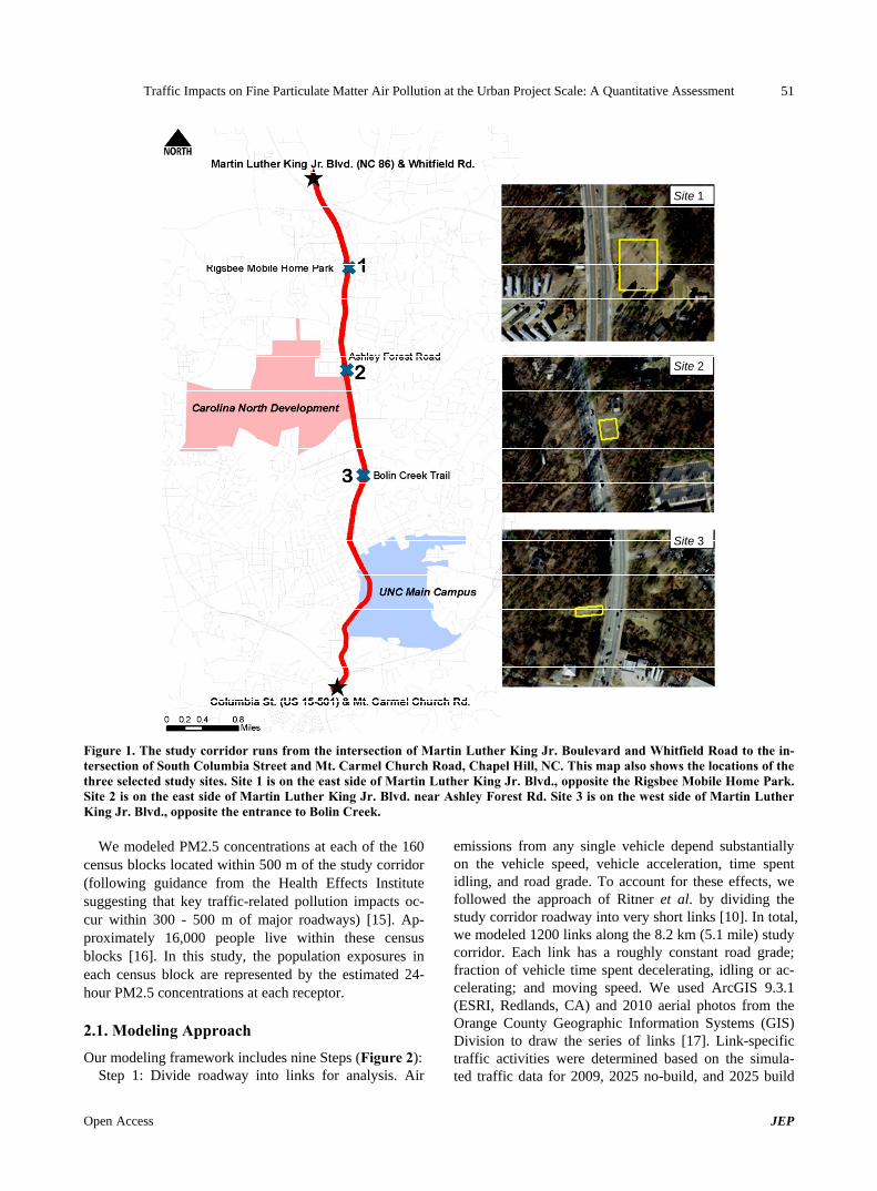
demonstrating the new modeling method is known as “Carolina North,” which is planned as an extension to the current UNC campus. UNC-Chapel Hill is the oldest public university in the United States and has a current student population of more than 29,000 [11]. The campus is located in the town of Chapel Hill, which has a popu-lation just over 57,000 [12]. The planned new campus will be located about 3 km (2 miles) north of the existing campus (Figure 1). If constructed, it is expected to in-crease the number of trips to the area by 10,000 per day by 2015—half of those by private vehicle—and, accord-ingly, to substantially increase traffic in the surrounding neighborhoods [13]. By 2025, the number of additional daily trips to the campus is expected to increase by as many as 40,000 [13]. The main traffic effects are ex-pected along Martin Luther King Jr. Boulevard, the main thoroughfare connecting the new campus to both the ex-isting campus (to the south) and the nearest highway in-terchange (to the north).

UNC commissioned a transportation impact analysis in 2009 in order to estimate the anticipated increases in traffic volumes, but the air quality impacts of the in-creased traffic were not evaluated. Hence, the transporta-tion impact analysis cannot be used directly to support decision-making about whether alternative transportation network designs (including, for example, new or ex-panded public transit routes) may be needed to prevent traffic-related air quality degradation and associated health impacts. By quantifying the air quality effects of additional traffic generated by the future campus, this paper can support a future quantitative HIA to inform local transportation and planning decisions.

2. Materials and Methods

Our process for modeling population exposure to excess PM2.5 attributable specifically to increased traffic from the Carolina North campus builds on a new approach recommended by Ritner et al. [10], who proposed an algorithm to account for vehicle acceleration, decelera-tion, and idling at intersections in modeling of near- roadway pollutant concentrations. We improved on the Ritner et al. approach by developing a new algorithm for incorporating hourly temperature variability in the esti-mation. We then tested our predictions against roadside air quality measurements. We analyzed near-roadway air quality for three different scenarios: 2009 conditions, 2025 conditions assuming the new campus is not built, and 2025 conditions assuming the campus is built. In-formation on traffic counts for all these scenarios came from the previously completed transportation impact analysis [14]. We modeled air quality effects only for daytime traffic (6 a.m. to 7 p.m.), since we assume that the major impacts will occur during these hours.

Open Access JEP


Open Access JEP

51

Site 2

Site 3

Site 1

Figure 1. The study corridor runs from the intersection of Martin Luther King Jr. Boulevard and Whitfield Road to the in-tersection of South Columbia Street and Mt. Carmel Church Road, Chapel Hill, NC. This map also shows the locations of the three selected study sites. Site 1 is on the east side of Martin Luther King Jr. Blvd., opposite the Rigsbee Mobile Home Park. Site 2 is on the east side of Martin Luther King Jr. Blvd. near Ashley Forest Rd. Site 3 is on the west side of Martin Luther King Jr. Blvd., opposite the entrance to Bolin Creek.

We modeled PM2.5 concentrations at each of the 160 census blocks located within 500 m of the study corridor (following guidance from the Health Effects Institute suggesting that key traffic-related pollution impacts oc-cur within 300 - 500 m of major roadways) [15]. Ap-proximately 16,000 people live within these census blocks [16]. In this study, the population exposures in each census block are represented by the estimated 24- hour PM2.5 concentrations at each receptor.

2.1. Modeling Approach

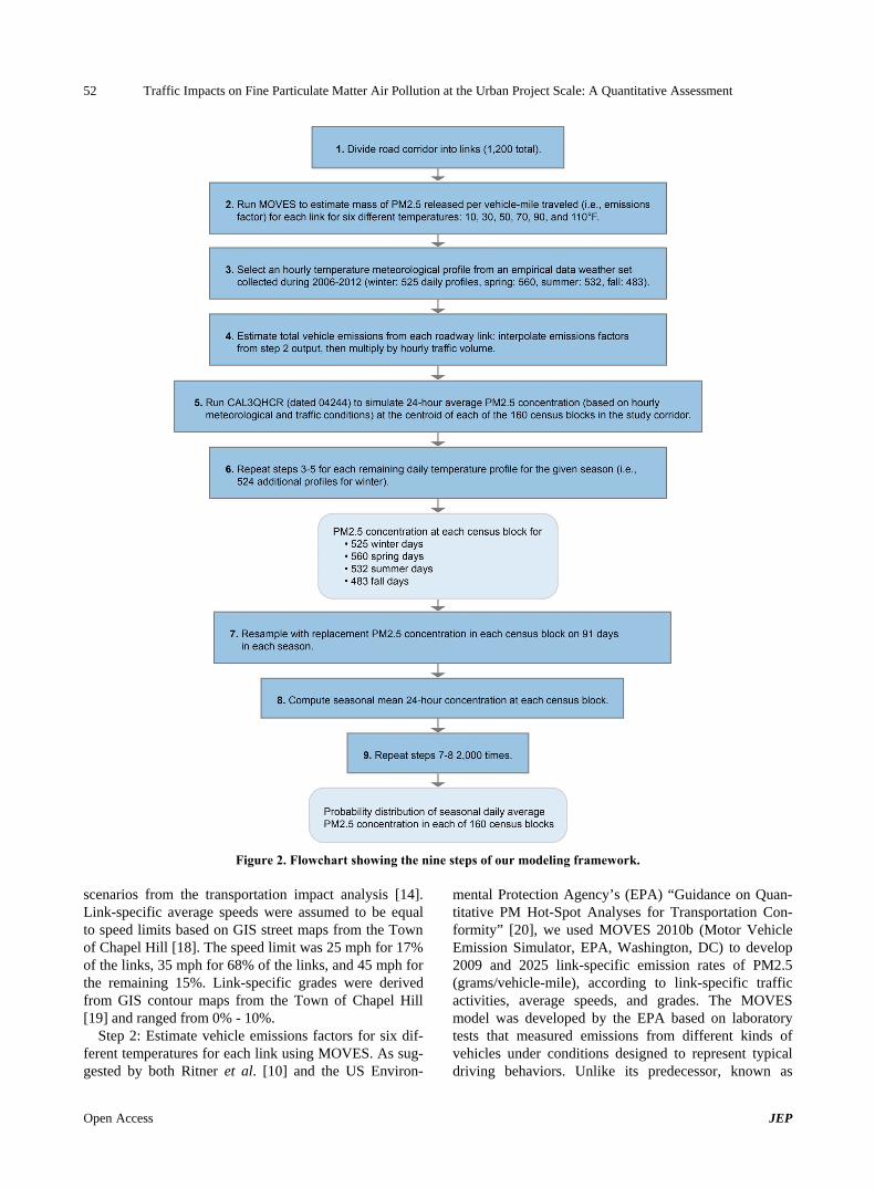
Our modeling framework includes nine Steps (Figure 2): Step 1: Divide roadway into links for analysis. Air

emissions from any single vehicle depend substantially on the vehicle speed, vehicle acceleration, time spent idling, and road grade. To account for these effects, we followed the approach of Ritner et al. by dividing the study corridor roadway into very short links [10]. In total, we modeled 1200 links along the 8.2 km (5.1 mile) study corridor. Each link has a roughly constant road grade; fraction of vehicle time spent decelerating, idling or ac-celerating; and moving speed. We used ArcGIS 9.3.1 (ESRI, Redlands, CA) and 2010 aerial photos from the Orange County Geographic Information Systems (GIS) Division to draw the series of links [17]. Link-specific traffic activities were determined based on the simulated traffic data for 2009, 202 no-build, and 2025 build 5


Figure 2. Flowchart showing the nine steps of our modeling framework. scenarios from the transportation impact analysis [14]. Link-specific average speeds were assumed to be equal to speed limits based on GIS street maps from the Town of Chapel Hill [18]. The speed limit was 25 mph for 17% of the links, 35 mph for 68% of the links, and 45 mph for the remaining 15%. Link-specific grades were derived from GIS contour maps from the Town of Chapel Hill [19] and ranged from 0% - 10%.

Step 2: Estimate vehicle emissions factors for six dif-ferent temperatures for each link using MOVES. As sug-gested by both Ritner et al. [10] and the US Environ-

mental Protection Agency’s (EPA) “Guidance on Quan-titative PM Hot-Spot Analyses for Transportation Con-formity” [20], we used MOVES 2010b (Motor Vehicle Emission Simulator, EPA, Washington, DC) to develop 2009 and 2025 link-specific emission rates of PM2.5 (grams/vehicle-mile), according to link-specific traffic activities, average speeds, and grades. The MOVES model was developed by the EPA based on laboratory tests that measured emissions from different kinds of vehicles under conditions designed to represent typical driving behaviors. Unlike its predecessor, known as

Open Access JEP


MOBILE6, MOVES can provide separate emissions factors for different vehicle operation modes: accelera-tion, deceleration, idling, and cruising [10].

MOVES models emissions for 13 vehicle types: mo-torcycle, passenger car, passenger truck, light commer-cial truck, intercity bus, transit bus, school bus, refuse truck, single unit short-haul truck, single unit long-haul truck, motor home, combination short-haul truck, and combination long-haul truck. It also considers three fuel types: gasoline, diesel, and compressed natural gas. Hence, in order for the model to provide accurate esti-mates for any specific roadway segment, the fraction of vehicles in each class and fuel type category must be estimated. For this analysis, we used vehicle fleet distri-bution data from Guilford County, NC [21] (county seat: Greensboro), since data specific to Chapel Hill were un-available. The fuel type distributions as well as fuel sup-ply and formulation in the project areas were based on national defaults. These data (fleet distributions and fuel types) were fixed in all MOVES runs.

The EPA’s PM hot-spot guidance recommends that the link-specific emission rates should be prepared based on average temperatures for four different time periods in a day for each season, meaning that each development scenario would require 16 MOVES runs. However, this approach does not fully account for daily temperature variability within a given season. Previous studies have shown that PM emission rates are highlight sensitive to temperature, and hence omitting temperature variability could decrease the accuracy of modeled emissions factors [22,23]. Our new algorithm for representing intra-seasonal variability in temperature and meteorological con-ditions runs MOVES for six different temperatures: 10, 30˚F, 50˚F, 70˚F, 90˚F, and 110˚F [24]. Later steps of the algorithm (described below) interpolate between these six estimates to determine temperature-specific emissions factors for each roadway link. For example, if a winter-time simulation of any given hour yielded a temperature of 40 degrees for that hour, we then estimated the vehicle emissions factors to be the average of the emissions fac-tors for 30 and 50 degrees.

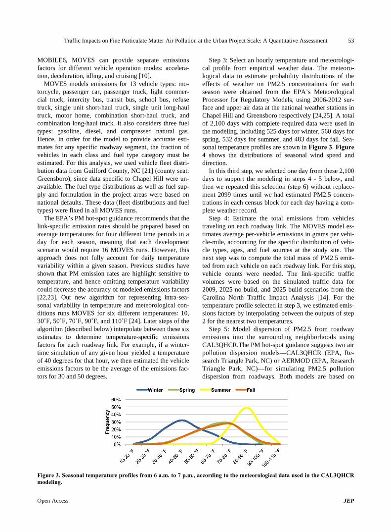
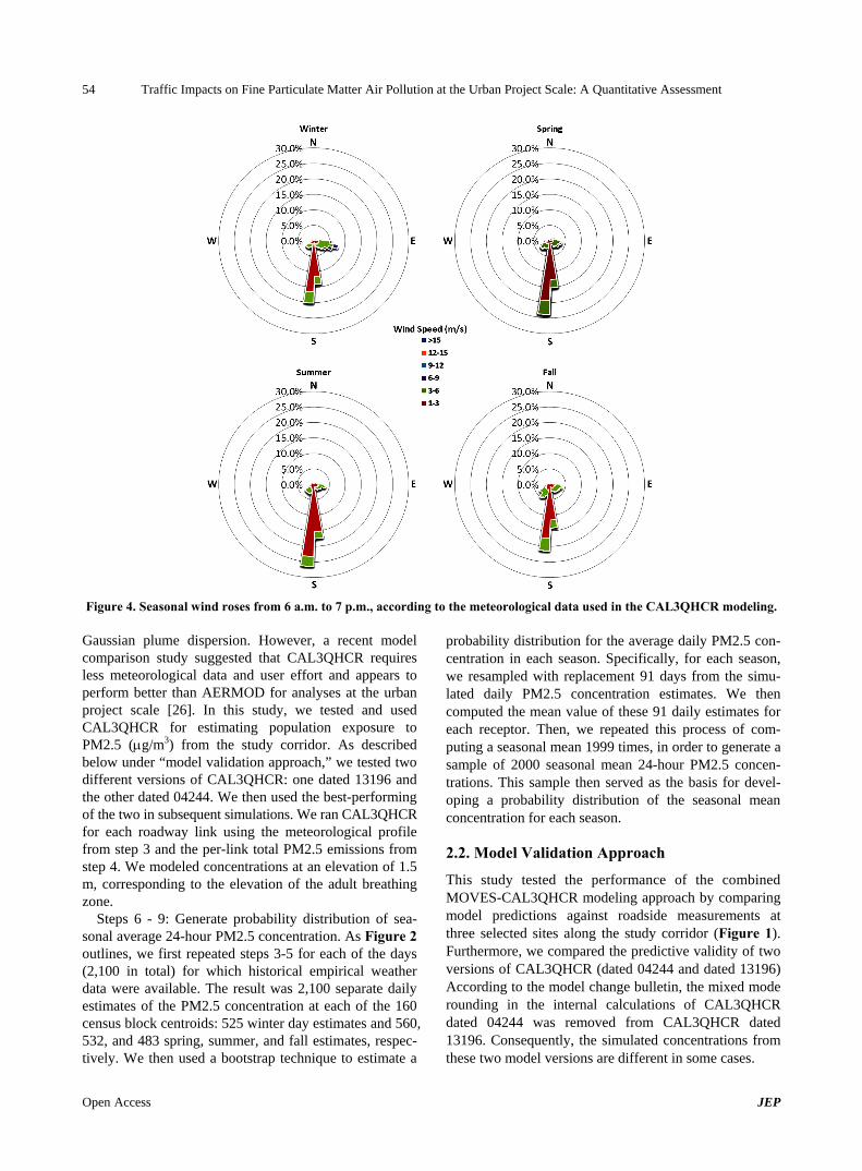
Step 3: Select an hourly temperature and meteorologi-cal profile from empirical weather data. The meteoro-logical data to estimate probability distributions of the effects of weather on PM2.5 concentrations for each season were obtained from the EPA’s Meteorological Processor for Regulatory Models, using 2006-2012 sur-face and upper air data at the national weather stations in Chapel Hill and Greensboro respectively [24,25]. A total of 2,100 days with complete required data were used in the modeling, including 525 days for winter, 560 days for spring, 532 days for summer, and 483 days for fall. Sea-sonal temperature profiles are shown in Figure 3. Figure 4 shows the distributions of seasonal wind speed and direction.

In this third step, we selected one day from these 2,100 days to support the modeling in steps 4 - 5 below, and then we repeated this selection (step 6) without replace-ment 2099 times until we had estimated PM2.5 concen-trations in each census block for each day having a com-plete weather record.

Step 4: Estimate the total emissions from vehicles traveling on each roadway link. The MOVES model es-timates average per-vehicle emissions in grams per vehi-cle-mile, accounting for the specific distribution of vehi-cle types, ages, and fuel sources at the study site. The next step was to compute the total mass of PM2.5 emit-ted from each vehicle on each roadway link. For this step, vehicle counts were needed. The link-specific traffic volumes were based on the simulated traffic data for 2009, 2025 no-build, and 2025 build scenarios from the Carolina North Traffic Impact Analysis [14]. For the temperature profile selected in step 3, we estimated emis-sions factors by interpolating between the outputs of step 2 for the nearest two temperatures.

Step 5: Model dispersion of PM2.5 from roadway emissions into the surrounding neighborhoods using CAL3QHCR.The PM hot-spot guidance suggests two air pollution dispersion models—CAL3QHCR (EPA, Re-search Triangle Park, NC) or AERMOD (EPA, Research Triangle Park, NC)—for simulating PM2.5 pollution dispersion from roadways. Both models are based on

Figure 3. Seasonal temperature profiles from 6 a.m. to 7 p.m., according to the meteorological data used in the CAL3QHCR modeling.

Open Access JEP


Figure 4. Seasonal wind roses from 6 a.m. to 7 p.m., according to the meteorological data used in the CAL3QHCR modeling. Gaussian plume dispersion. However, a recent model comparison study suggested that CAL3QHCR requires less meteorological data and user effort and appears to perform better than AERMOD for analyses at the urban project scale [26]. In this study, we tested and used CAL3QHCR for estimating population exposure to PM2.5 (g/m3) from the study corridor. As described below under “model validation approach,” we tested two different versions of CAL3QHCR: one dated 13196 and the other dated 04244. We then used the best-performing of the two in subsequent simulations. We ran CAL3QHCR for each roadway link using the meteorological profile from step 3 and the per-link total PM2.5 emissions from step 4. We modeled concentrations at an elevation of 1.5 m, corresponding to the elevation of the adult breathing zone.

Steps 6 - 9: Generate probability distribution of sea-sonal average 24-hour PM2.5 concentration. As Figure 2 outlines, we first repeated steps 3-5 for each of the days (2,100 in total) for which historical empirical weather data were available. The result was 2,100 separate daily estimates of the PM2.5 concentration at each of the 160 census block centroids: 525 winter day estimates and 560, 532, and 483 spring, summer, and fall estimates, respec-tively. We then used a bootstrap technique to estimate a

probability distribution for the average daily PM2.5 con-centration in each season. Specifically, for each season, we resampled with replacement 91 days from the simu-lated daily PM2.5 concentration estimates. We then computed the mean value of these 91 daily estimates for each receptor. Then, we repeated this process of com-puting a seasonal mean 1999 times, in order to generate a sample of 2000 seasonal mean 24-hour PM2.5 concen-trations. This sample then served as the basis for devel-oping a probability distribution of the seasonal mean concentration for each season.

2.2. Model Validation Approach

This study tested the performance of the combined MOVES-CAL3QHCR modeling approach by comparing model predictions against roadside measurements at three selected sites along the study corridor (Figure 1). Furthermore, we compared the predictive validity of two versions of CAL3QHCR (dated 04244 and dated 13196) According to the model change bulletin, the mixed mode rounding in the internal calculations of CAL3QHCR dated 04244 was removed from CAL3QHCR dated 13196. Consequently, the simulated concentrations from these two model versions are different in some cases.

Open Access JEP


We used a DustTrak DRX Aerosol Monitor Model 8534 (TSI, Shoreview, MN) to measure total PM2.5 con-centrations at each of the three sites The DustTrak DRX instrument or similar models have been used in roadside measurements in several previous studies [27-29]. The DustTrak can detect concentrations from 1 to 150,000 g/m3 with an error of 0.1% of the monitored concen-tration [30]. All of these instruments are calibrated at the factory with a known mass concentration of Arizona Test Dust (ISO 12103-1, A1 test dust) [31]. In addition, in each sampling period, we calibrated the instrument be-fore taking measurements. During all sampling events, the DustTrak was held about 1.5 m above the ground (the adult breathing zone height) and programmed to record the total concentration every five seconds.

We collected samples on two separate days at Site 1 and on one day at Sites 2 and 3 for a total of four sam-pling days in the study corridor. During three of the four sampling days, we monitored PM2.5 concentrations dur-ing the morning and evening peak traffic periods and also in the middle of the day four an hour at a time (roughly 8:00 - 9:00 a.m., noon-1:00 p.m., and 5:00 - 6:00 p.m.). At Site 2, the property owner requested that we not col-lect samples in the evening, so we only sampled during the morning and noon hours. Table 1 shows sample col-lection dates and measured PM2.5 concentrations.

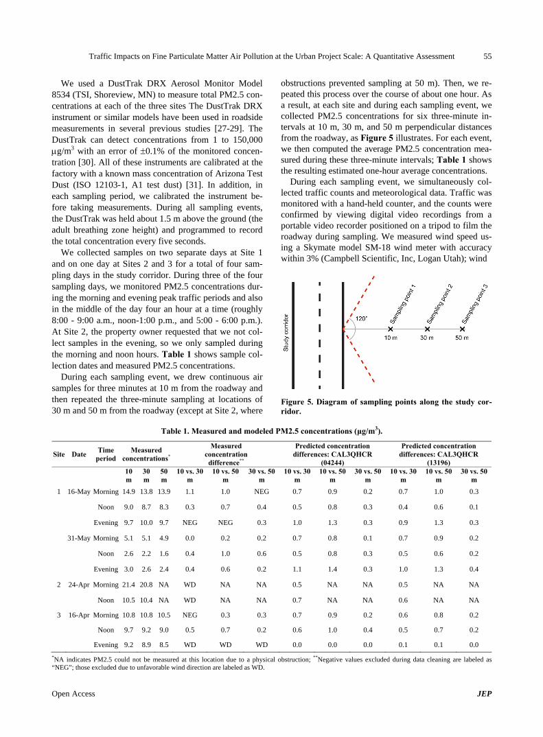
During each sampling event, we drew continuous air samples for three minutes at 10 m from the roadway and then repeated the three-minute sampling at locations of 30 m and 50 m from the roadway (except at Site 2, where

obstructions prevented sampling at 50 m). Then, we re-peated this process over the course of about one hour. As a result, at each site and during each sampling event, we collected PM2.5 concentrations for six three-minute in-tervals at 10 m, 30 m, and 50 m perpendicular distances from the roadway, as Figure 5 illustrates. For each event, we then computed the average PM2.5 concentration measured during these three-minute intervals; Table 1 shows the resulting estimated one-hour average concentrations.

During each sampling event, we simultaneously col-lected traffic counts and meteorological data. Traffic was monitored with a hand-held counter, and the counts were confirmed by viewing digital video recordings from a portable video recorder positioned on a tripod to film the roadway during sampling. We measured wind speed us-ing a Skymate model SM-18 wind meter with accuracy within 3% (Campbell Scientific, Inc, Logan Utah); wind

Figure 5. Diagram of sampling points along the study cor-idor. r

Table 1. Measured and modeled PM2.5 concentrations (μg/m3).

Site Date Time

period Measured

concentrations*

Measured concentration difference**

Predicted concentration differences: CAL3QHCR

(04244)

Predicted concentration differences: CAL3QHCR

(13196)

10 m

30 m

50 m

10 vs. 30 m

10 vs. 50 m

30 vs. 50 m

10 vs. 30 m

10 vs. 50 m

30 vs. 50 m

10 vs. 30 m

10 vs. 50 m

30 vs. 50 m

1 16-May Morning 14.9 13.8 13.9 1.1 1.0 NEG 0.7 0.9 0.2 0.7 1.0 0.3

Noon 9.0 8.7 8.3 0.3 0.7 0.4 0.5 0.8 0.3 0.4 0.6 0.1

Evening 9.7 10.0 9.7 NEG NEG 0.3 1.0 1.3 0.3 0.9 1.3 0.3

31-May Morning 5.1 5.1 4.9 0.0 0.2 0.2 0.7 0.8 0.1 0.7 0.9 0.2

Noon 2.6 2.2 1.6 0.4 1.0 0.6 0.5 0.8 0.3 0.5 0.6 0.2

Evening 3.0 2.6 2.4 0.4 0.6 0.2 1.1 1.4 0.3 1.0 1.3 0.4

2 24-Apr Morning 21.4 20.8 NA WD NA NA 0.5 NA NA 0.5 NA NA

Noon 10.5 10.4 NA WD NA NA 0.7 NA NA 0.6 NA NA

3 16-Apr Morning 10.8 10.8 10.5 NEG 0.3 0.3 0.7 0.9 0.2 0.6 0.8 0.2

Noon 9.7 9.2 9.0 0.5 0.7 0.2 0.6 1.0 0.4 0.5 0.7 0.2

Evening 9.2 8.9 8.5 WD WD WD 0.0 0.0 0.0 0.1 0.1 0.0

*NA indicates PM2.5 could not be measured at this location due to a physical obstruction; **Negative values excluded during data cleaning are labeled as NEG”; those excluded due to unfavorable wind direction are labeled as WD. “

Open Access JEP


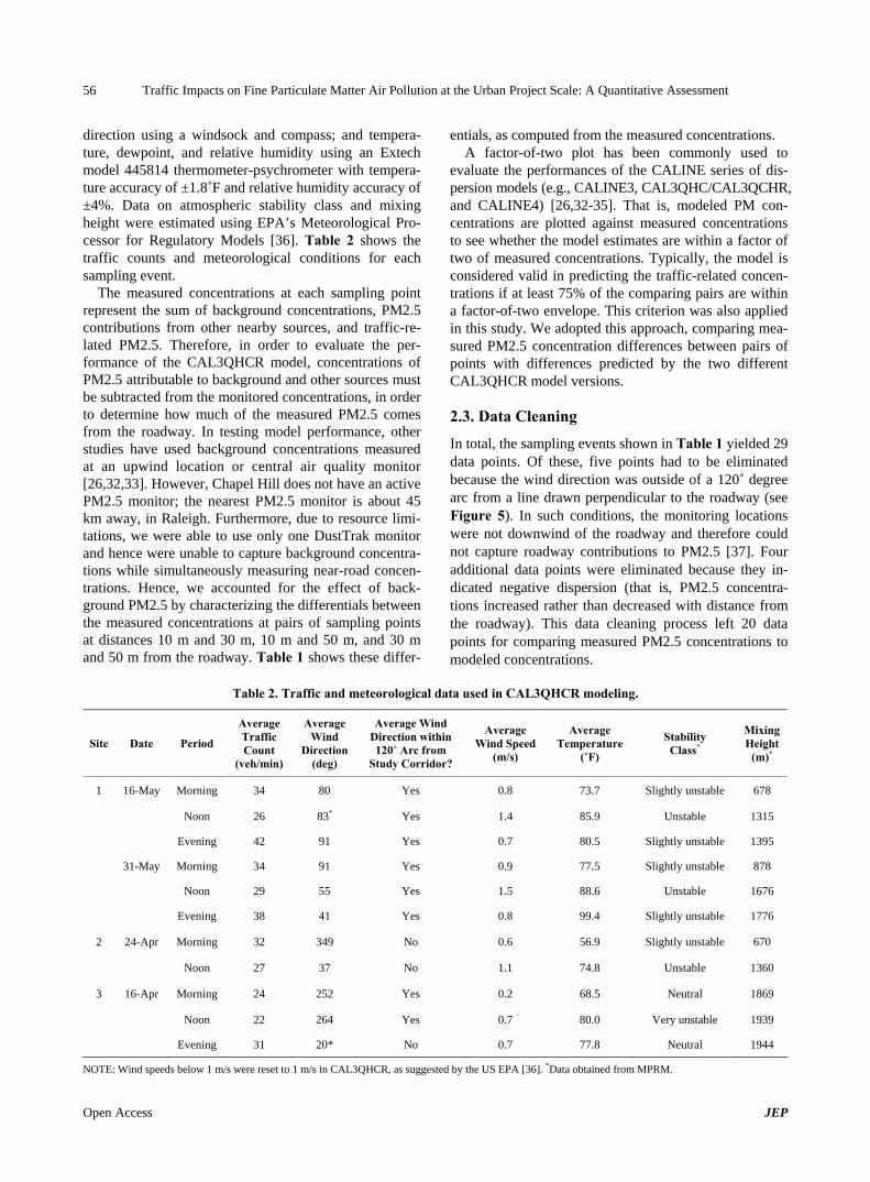
direction using a windsock and compass; and tempera-ture, dewpoint, and relative humidity using an Extech model 445814 thermometer-psychrometer with tempera-ture accuracy of ±1.8˚F and relative humidity accuracy of ±4%. Data on atmospheric stability class and mixing height were estimated using EPA’s Meteorological Pro- cessor for Regulatory Models [36]. Table 2 shows the traffic counts and meteorological conditions for each sampling event.

The measured concentrations at each sampling point represent the sum of background concentrations, PM2.5 contributions from other nearby sources, and traffic-related PM2.5. Therefore, in order to evaluate the per-formance of the CAL3QHCR model, concentrations of PM2.5 attributable to background and other sources must be subtracted from the monitored concentrations, in order to determine how much of the measured PM2.5 comes from the roadway. In testing model performance, other studies have used background concentrations measured at an upwind location or central air quality monitor [26,32,33]. However, Chapel Hill does not have an active PM2.5 monitor; the nearest PM2.5 monitor is about 45 km away, in Raleigh. Furthermore, due to resource limi-tations, we were able to use only one DustTrak monitor and hence were unable to capture background concentra-tions while simultaneously measuring near-road concen-trations. Hence, we accounted for the effect of back-ground PM2.5 by characterizing the differentials between the measured concentrations at pairs of sampling points at distances 10 m and 30 m, 10 m and 50 m, and 30 m and 50 m from the roadway. Table 1 shows these differ-

entials, as computed from the measured concentrations. A factor-of-two plot has been commonly used to

evaluate the performances of the CALINE series of dis-persion models (e.g., CALINE3, CAL3QHC/CAL3QCHR, and CALINE4) [26,32-35]. That is, modeled PM con-centrations are plotted against measured concentrations to see whether the model estimates are within a factor of two of measured concentrations. Typically, the model is considered valid in predicting the traffic-related concen-trations if at least 75% of the comparing pairs are within a factor-of-two envelope. This criterion was also applied in this study. We adopted this approach, comparing measured PM2.5 concentration differences between pairs of points with differences predicted by the two different CAL3QHCR model versions.

2.3. Data Cleaning

In total, the sampling events shown in Table 1 yielded 29 data points. Of these, five points had to be eliminated because the wind direction was outside of a 120˚ degree arc from a line drawn perpendicular to the roadway (see Figure 5). In such conditions, the monitoring locations were not downwind of the roadway and therefore could not capture roadway contributions to PM2.5 [37]. Four additional data points were eliminated because they in-dicated negative dispersion (that is, PM2.5 concentra-tions increased rather than decreased with distance from the roadway). This data cleaning process left 20 data points for comparing measured PM2.5 concentrations to modeled concentrations.

Table 2. Traffic and meteorological data used in CAL3QHCR modeling.

Site Date Period

Average Traffic Count

(veh/min)

Average Wind

Direction (deg)

Average Wind Direction within 120˚ Arc from

Study Corridor?

Average Wind Speed

(m/s)

Average Temperature

(˚F)

Stability Class*

MixingHeight

(m)*

1 16-May Morning 34 80 Yes 0.8 73.7 Slightly unstable 678

Noon 26 83* Yes 1.4 85.9 Unstable 1315

Evening 42 91 Yes 0.7 80.5 Slightly unstable 1395

31-May Morning 34 91 Yes 0.9 77.5 Slightly unstable 878

Noon 29 55 Yes 1.5 88.6 Unstable 1676

Evening 38 41 Yes 0.8 99.4 Slightly unstable 1776

2 24-Apr Morning 32 349 No 0.6 56.9 Slightly unstable 670

Noon 27 37 No 1.1 74.8 Unstable 1360

3 16-Apr Morning 24 252 Yes 0.2 68.5 Neutral 1869

Noon 22 264 Yes 0.7 80.0 Very unstable 1939

Evening 31 20* No 0.7 77.8 Neutral 1944

N OTE: Wind speeds below 1 m/s were reset to 1 m/s in CAL3QHCR, as suggested by the US EPA [36]. *Data obtained from MPRM.

Open Access JEP


3. Results

3.1. Vehicle Emission Rates

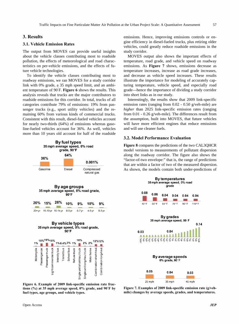
The output from MOVES can provide useful insights about the vehicle classes contributing most to roadside pollution, the effects of meteorological and road charac-teristics on per-vehicle emissions, and the effects of fu-ture vehicle technologies.

To identify the vehicle classes contributing most to roadway emissions, we ran MOVES for a study corridor link with 0% grade, a 35 mph speed limit, and an ambi-ent temperature of 90˚F. Figure 6 shows the results. This analysis reveals that trucks are the major contributors to roadside emissions for this corridor. In total, trucks of all categories contribute 79% of emissions: 19% from pas-senger trucks (e.g., sport utility vehicles) and the re-maining 60% from various kinds of commercial trucks. Consistent with this result, diesel-fueled vehicles account for nearly two-thirds (64%) of emissions whereas gaso-line-fueled vehicles account for 36%. As well, vehicles more than 10 years old account for half of the roadside

Figure 6. Example of 2009 link-specific emission rate frac-tions (%) at 35 mph average speed, 0% grade, and 90˚F by fuel types, age groups, and vehicle types.

emissions. Hence, improving emissions controls or en-gine efficiency in diesel-fueled trucks, plus retiring older vehicles, could greatly reduce roadside emissions in the study corridor.

MOVES output also shows the important effects of temperature, road grade, and vehicle speed on roadway emissions. As Figure 7 shows, emissions decrease as temperature increases, increase as road grade increases, and decrease as vehicle speed increases. These results illustrate the importance for modeling of accurately cap-turing temperature, vehicle speed, and especially road grade—hence the importance of dividing a study corridor into short links as in our study.

Interestingly, the results show that 2009 link-specific emission rates (ranging from 0.02 - 0.50 g/veh-mile) are higher than 2025 link-specific emission rates (ranging from 0.01 - 0.26 g/veh-mile). The differences result from the assumption, built into MOVES, that future vehicles will have more efficient engines that reduce emissions and will use cleaner fuels.

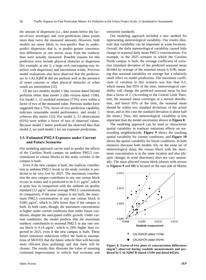
3.2. Model Performance Evaluation

Figure 8 compares the predictions of the two CAL3QHCR model versions to measurements of pollutant dispersion along the roadway corridor. The figure also shows the “factor-of-two envelope:” that is, the range of predictions that are within a factor of two of the measured dispersion. As shown, the models contain both under-predictions of

Figure 7. Examples of 2009 link-specific emission rate (g/veh- mile) changes by average speeds, grades, and temperatures.

Open Access JEP


the amount of dispersion (i.e., data points below the fac-tor-of-two envelope) and over-predictions (data points more than twice the measured amount). However, both models are more likely to over-predict than to under- predict dispersion: that is, to predict greater concentra-tion differences as one moves away from the roadway than were actually measured. Possible reasons for this prediction error include physical obstacles to dispersion (for example, at site 3, a large rock outcropping may in-terfere with dispersion) and intermittent winds. Previous model evaluations also have observed that the predeces-sor to CAL3QHCR did not perform well in the presence of street canyons or other physical obstacles or when winds are intermittent [32].

Of the two models, model 1 (the version dated 04244) performs better than model 2 (the version dated 1196). For model 1, 15 modeled estimates (75%) were within a factor of two of the measured value. Previous studies have suggested that a 75%, factor-of-two prediction capability indicates reasonable model performance, and model 1 achieves this metric [32]. For model 2, 13 observations (65%) were within a factor of two of observed values. Because model 1 better predicted the observed data than model 2, we used model 1 for our exposure predictions.

3.3. Estimated PM2.5 Exposure under Current and Future Scenarios

Our modeling approach can be used to predict the effects of the Carolina North campus on ambient PM2.5 con-centrations in census blocks in the study corridor if the campus is built.

Even if the new campus is built, the roadway contribu-tion to ambient PM2.5 levels in the study corridor is pre-dicted to be very low by 2025. The maximum contribu-tion the new campus contributes to any one census block occurs in winter and is predicted to be 0.11 µg/m3, which is quite low in comparison with the ambient air quality standard (12 µg/m3 annual average PM2.5 concentration). In comparison, if the new campus is not built, the maxi-mum PM2.5 concentration in any one census block is 0.085 µg/m3, which is 24% lower than if the campus is built. In both cases, though, the maximum concentration is higher under current conditions than under future con-ditions, despite the anticipated traffic growth. Under cur-rent conditions, the model predicts that the maximum roadway contribution to seasonal PM2.5 in any one cen-sus block is 0.14 µg/m3, which is 24% higher than ex-pected in 2025, even if the new campus is built. These future emissions reductions reflect the built-in assump-tions of MOVES that the future vehicle fleet will become more efficient (less polluting) and that fuels will be cleaner. The results thus illustrate the value of ensuring continued improvements in vehicle fuel economy and

emissions standards. Our modeling approach included a new method for

representing meteorological variability. Our results illus-trate that variability can be important in some locations. Overall, the daily meteorological variability caused little change in seasonal daily mean PM2.5 concentrations. For example, in the 2025 scenario in which the Carolina North campus is built, the average coefficient of varia-tion (standard deviation of the predicted seasonal mean divided by average of the seasonal mean) is 0.06, mean-ing that seasonal variability on average has a relatively small effect on model predictions. The maximum coeffi-cient of variation in this scenario was less than 0.5, which means that 95% of the time, meteorological vari-ability will change the predicted seasonal mean by less than a factor of 2. (According to the Central Limit Theo-rem, the seasonal mean converges to a normal distribu-tion, and hence 95% of the time, the seasonal mean should be within two standard deviations of the actual mean, and in this case the standard deviation is about half the mean.) Thus, this meteorological variability is less important than the model uncertainty shown in Figure 8.

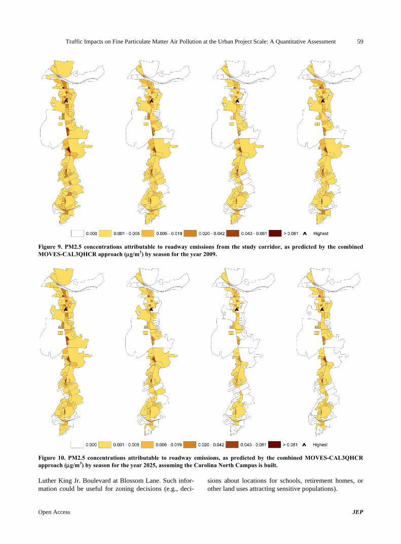
The modeling approach can be used to characterize spatial variability in roadway emissions effects on sur-rounding neighborhoods. Figure 9 shows the resulting spatial variability for current conditions, and Figure 10 shows the spatial variability for future conditions. In both instances (because both models rely on the same set of meteorological data), the census block with the maxi-mum concentration is in the same location and also (de-spite changes in wind directions) does not vary season-ally. The most affected census block (shown with arrows in Figures 9 and 10) is located on the east side of Martin

Figure 8. Factor-of-two plots of concentration differences (mg/m3) observed during roadside measurements and pre-

icted by CAL3QHCR (dated 13196 and dated 04244). d

Open Access JEP


Open Access JEP

59

Figure 9. PM2.5 concentrations attributable to roadway emissions from the study corridor, as predicted by the combined MOVES-CAL3QHCR approach (g/m3) by season for the year 2009.

Figure 10. PM2.5 concentrations attributable to roadway emissions, as predicted by the combined MOVES-CAL3QHCR approach (g/m3) by season for the year 2025, assuming the Carolina North Campus is built. Luther King Jr. Boulevard at Blossom Lane. Such infor-mation could be useful for zoning decisions (e.g., deci-

sions about locations for schools, retirement homes, or other land uses attracting sensitive populations).


4. Discussion

Our results are consistent with the few empirical evalua-tions of the accuracy in predicting roadway PM2.5 con-centrations of CAL3QHCR and its predecessor, known as CALINE. Yura et al. compared CALINE predictions of PM2.5 to measured PM2.5 concentrations at a busy intersection in a suburban community in Sacramento, California, and an urban site along a six-lane road in London, England [32]. They found that 80% of model predictions were within a factor-of-two envelope of meas-ured concentrations at the suburban site but that only 56% of predictions were within the factor-of-two enve-lope for the urban site. They attributed the poor per-formance at the urban site to limitations of the emissions factors they used (they relied on scaling United Kingdom PM10 emissions factors) and to street canyon effects. Chen et al. extended Yura’s work by comparing the per-formance of the CAL3QHC model to that of the CALINE model for the same two sites (although during a different time period) as Yura used [26]. Chen et al. found that predicted PM2.5 concentrations were within the factor-of-two envelope for 69% of the Sacramento data points and for 59% of the London data points. In both cities, CAL3QHC outperformed CALINE. Gokhale and Raokhande compared the CALINE and CAL3QHC models’ ability to predict roadside PM2.5 concentrations at a busy intersection in Guwahati, India [38]. They found that the CAL3QHC model predictions were within a factor-of-two envelope for 65% of (66 of 102) hourly PM2.5 observations during winter and that the CAL3QHC model outperformed the CALINE model (the latter of which produced predictions within the factor-of-two en-velope for 46 of 102 data points).

Our findings about the amount of PM2.5 contributed to a given location by a single busy roadway also are consistent with findings of the few modeling studies and quantitative HIAs of local effects of traffic in the United States. In a modeling study, Zhang and Batterman used CALINE along with the predecessor to MOVES, known as MOBILE6.2, to estimate the amount of PM2.5 pollu-tion contributed by a busy roadway in Detroit, Michigan [33]. They found that the local roadway contributed only a small amount of the measured PM2.5: total measured PM2.5 concentrations averaged 16.8 µg/m3, but Zhang and Batterman attributed “no more than 0.5 µg/m3” to the roadway. They attributed the majority of observed PM2.5 “to long range transport of sulfate and other aerosols from the Ohio River Valley.” Chen et al. also found that roadways in Sacramento and London contributed rela-tively small fractions to observed PM2.5 concentrations at the study sites [26].

Of the four transportation-related quantitative HIAs identified in the comprehensive review by Bhatia and

Seto et al., three predicted PM2.5 concentrations attrib-utable to vehicles on roadways (the fourth predicted PM10 concentrations) [9]. All of these HIAs (including the HIA that estimated PM10 concentrations) focused on proposed new development projects in or near Oakland, California, and all used CAL3QHCR to support their predictions. The first, an HIA of a proposed residential development to be constructed near a highway (with an average daily traffic volume of about 119,000 vehicles) in Pittsburg, California, used CAL3QHCR to estimate that traffic-attributable exposures adjacent to the high-way are about 2 µg/m3 but that these exposures decline rapidly with distance to about 0.2 µg/m3 [39]; this esti-mate assumed a constant emissions factor of 0.15 g/vehicle-mile travelled, whereas our estimate employed MOVES to estimate link-specific emissions factors, re-sulting in a range of emissions factors of 0.02 - 0.5 g/vehicle-mile travelled. The second of these three quan-titative HIAs considered the potential traffic-related health effects of potential affordable housing sites in Oakland, California; this HIA used CAL3QHCR to estimate that two major roadways with combined annual average daily traffic counts of about 225,000 vehicles would contribute about 0.4 - 0.5 µg/m3 to PM2.5 exposures at the locations under consideration, all of which were within meters of the roadways [40]. The third HIA concerned a potential new residential development near a transit station in Oakland; it estimated that alongside a major highway (with daily traffic counts averaging 144,000 vehicles) neighboring the proposed development site, about 0.3 µg/m3 of PM2.5 could be attributed to traffic but that this traffic-related contribution decreased to 0.1 µg/m3 at a distance of 150 m from the highway [41]. In summary, these HIAs estimate that directly adjacent to highways running through the Oakland area, traffic contributes anywhere from about 0.3 - 2 µg/m3. All of these high-ways have daily traffic counts at least five times as high as the current traffic along the roadway corridor analyzed in the present study. The estimated roadway contributions that our modeling approach yielded (with the maximum roadway-contributed concentration of 0.14 µg/m3 under current conditions) hence are quite consistent with these previous estimates when traffic volumes and distances of census block centroids to the roadway are considered. That is, if one multiplies the maximum estimate from our modeling approach by 5, then the estimated maximum predicted concentration in any census block in the study corridor is 0.7 µg/m3. This is within the range of concen-trations predicted in the California studies.

5. Conclusions

In this study, a new modeling framework to quantify the project traffic growth impacts on population exposure to

Open Access JEP


PM2.5 air pollution was proposed and then demonstrated by quantifying exposure to roadway PM2.5 emissions that may occur in the future due to the Carolina North development in Chapel Hill, North Carolina. This mod-eling framework should benefit others conducting quan-titative HIAs of the built environment and transportation projects. Whereas previous HIAs employing air disper-sion models have used average meteorological data and have assumed that vehicles move at a constant cruising speed along roadway links, our approach considers link- by-link variation in vehicle behavior and hourly mete-orological variability.

Our results reveal that improvements in vehicle tech-nologies and fuels will be a key factor in protecting pub-lic health from the air pollution generated by increases in traffic expected to occur due to local and regional devel-opments in the future. In fact, the models we employed predict that traffic-related PM2.5 in the study corridor may actually decrease in the future, even if traffic in-creases, due to improved vehicle technologies and fuels.

Our results also reveal the need for improve models to predict near-road PM2.5 concentrations. While the CAL3QHCR dispersion model was able to predict dis-persion reasonably well, about 25% of model predictions over-estimated dispersion. This overestimation bias re-sults in under-estimates of pollutant exposure. Hence, reducing model bias is critical to ensuring that deci-sion-makers are adequately informed about air quality and health risks associated with roadway traffic.

REFERENCES [1] J. Kemm, “Perspectives on Health Impact Assessment,”

Bulleting of the World Health Organization, Vol. 81, No. 6, 2003, p. 387.

[2] National Research Council, “Improving Health in the United States: The Role of Health Impact Assessment,” National Academy Press, Washington DC, 2011.

[3] A. Wernham, “Health Impact Assessments Are Needed in Decision Making about Environmental and Land-Use Po- licy,” Health Affairs (Project Hope), Vol. 30, No. 5, 2011, pp. 947-956. http://dx.doi.org/10.1377/hlthaff.2011.0050

[4] R. Lozano, M. Naghavi, K. Foreman, S. Lim, K. Shibuya, V. Aboyans and C. J. L. Murray, “Global and Regional Mortality from 235 Causes of Death for 20 Age Groups in 1990 and 2010: A Systematic Analysis for the Global Burden of Disease Study 2010,” Lancet, Vol. 380, No. 9859, 2012, pp. 2095-2128. http://dx.doi.org/10.1016/S0140-6736(12)61728-0

[5] A. L. Dannenberg, R. Bhatia, B. L. Cole, S. K. Heaton, J. D. Feldman and C. D. Rutt, “Use of Health Impact As- sessment in the U.S.: 27 Case Studies, 1999-2007,” Ame- rican Journal of Preventive Medicine, Vol. 34, No. 3, 2008, pp. 241-256. http://dx.doi.org/10.1016/j.amepre.2007.11.015

[6] M. Wismar, J. Blau, K. Ernst and J. Figueras, “The Effec-

tiveness of Health Impact Assessment: Scope and Limita- tions of Supporting Decision-Making in Europe,” Politi- cal Science, Copenhagen WHO Regional Office for Europe, 2007.

[7] R. Bhatia and M. Katz, “Estimation of Health Benefits from a Local Living Wage Ordinance,” American Journal of Public Health, Vol. 91, No. 9, 2001, pp. 1398-1402. http://dx.doi.org/10.2105/AJPH.91.9.1398

[8] L. Singleton-Baldrey, “The Impacts of Health Impact As- sessment: A Review of 54 Health Impact Assessments, 2007-2012,” University of North Carolina at Chapel Hill, Chapel Hill, 2012.

[9] R. Bhatia and E. Seto, “Quantitative Estimation in Health Impact Assessment: Opportunities and Challenges,” En- vironmental Impact Assessment Review, Vol. 31, No. 3, 2011, pp. 20301-20309. http://dx.doi.org/10.1016/j.eiar.2010.08.003

[10] M. Ritner, K. K. Westerlund, C. D. Cooper and M. Clag- gett, “Accounting for Acceleration and Deceleration Emis- sions in Intersection Dispersion Modeling Using MOVES and CAL3QHC,” Journal of the Air and Waste Manage- ment Association, Vol. 63, No. 6, 2013, pp. 724-736. http://dx.doi.org/10.1080/10962247.2013.778220

[11] University of North Carolina at Chapel Hill, “About UNC,” 2013. http://www.unc.edu/about/

[12] Town of Chapel Hill, “Snapshot of the Town of Chapel Hill,” 2012. http://www.townofchapelhill.org/Modules/ShowDocument.aspx?documentid=12177

[13] K. Ross, “Carolina North Hearing Highlights Traffic Im- pact,” The Carrboro Citizen, 2009. http://www.carrborocitizen.com/main/2009/05/14/carolina-north-hearing-highlights-traffic-impact/

[14] Vanasse Hangen Brustlin, Inc., “Transportation Impact Analysis for the Carolina North Development,” Water- town, 2009.

[15] Health Effects Institute, “Traffic-Related Air Pollution: A Critical Review of the Literature on Emissions, Exposure, and Health Effects,” HEI Special Report 17, Boston, 2010.

[16] US Census Bureau, “Census Block Shapefiles with 2010 Census Population and Housing Unit Counts,” 2011.

[17] Orange County, “Aerials 2010,” 2012.

[18] Town of Chapel Hill, “Street Centerline,” 2009.

[19] Town of Chapel Hill, “2ft Elevation Contours,” 2009.

[20] US Environmental Protection Agency, “Guidance on Quan- titative PM Hot-Spot Analyses for Transportation Con- formity,” 2011. http://www.epa.gov/otaq/stateresources/transconf/policy/pm-hotspot-guide.pdf

[21] N.C. Division of Air Quality, “MOVES Input and Output Giles: Hickory and Triad PM2.5 Redesignation Demon- stration and Maintenance Plan,” 2011.

[22] P. Mulawa, S. Cadle, H. Knapp, R. Zweidinger, R. Snow, R. Lucas and J. Goldbach, “Effect of Ambient Tempera- ture and E-10 Fuel on Primary Exhaust Particulate Matter Emissions from Light-Duty Vehicles,” Environmental

Open Access JEP

http://dx.doi.org/10.1377/hlthaff.2011.0050

http://dx.doi.org/10.1016/S0140-6736(12)61728-0

http://dx.doi.org/10.1016/j.amepre.2007.11.015

http://dx.doi.org/10.2105/AJPH.91.9.1398

http://dx.doi.org/10.1016/j.eiar.2010.08.003

http://dx.doi.org/10.1080/10962247.2013.778220


Open Access JEP

62

Science & Technology, Vo. 31, 1997, pp. 1302-1307. http://dx.doi.org/10.1021/es960514r

[23] D. Choi, M. Beardsley, D. Brzezinski, J. Koupal and J. Warila, “MOVES Sensitivity Analysis: The Impacts of Temperature and Humidity on Emissions,” The MOVES Workshop 2011, US Environmental Protection Agency, Ann Arbor, 2011.

[24] National Climatic Data Center, “Quality Controlled Local Climatological Data (QCLCD),” 2013.

[25] National Oceanic and Atmospheric Administration, “NOAA/ESRL Radiosonde Database,” 2013.

[26] H. Chen, S. Bai, D. Eisinger, D. Niemeier and M. Claggett, “Predicting Near-Road PM2.5 Concentrations,” Transportation Research Record: Journal of the Trans- portation Research Board, Vol. 2123, 2009, pp. 26-37. http://dx.doi.org/10.3141/2123-04

[27] M. G. Boarnet, D. Houston, R. Edwards, M. Princevac, G. Ferguson, H. Pan and C. Bartolome, “Fine Particulate Concentrations on Sidewalks in Five Southern California Cities,” Atmospheric Environment, Vol. 45, No. 24, 2011, pp. 4025-4033. http://dx.doi.org/10.1016/j.atmosenv.2011.04.047

[28] J. S. Wang, T. L. Chan, Z. Ning, C. W. Leung, C. S. Cheung and W. T. Hung, “Roadside Measurement and Prediction of CO and PM 2.5 Dispersion from On-Road Vehicles in Hong Kong,” Transportation Research Part D: Transport and Environment, Vol. 11, No. 4, 2006, pp. 242-249. http://dx.doi.org/10.1016/j.trd.2006.04.002

[29] Y. Wu, J. Hao, L. Fu, Z. Wang and U. Tang, “Vertical and Horizontal Profiles of Airborne Particulate Matter near Major Roads in Macao, China,” Atmospheric Envi- ronment, Vol. 36, No. 31, 2002, pp. 4907-4918. http://dx.doi.org/10.1016/S1352-2310(02)00467-3

[30] TSI, Inc., “Spec Sheet Model 8533/8534 DustTrak DRX Aerosol Monitor, 2012.

[31] TSI, Inc., “DustTrak DRX Aerosol Monitor Theory of Operation (EXPMN-002),” 2012.

[32] E. A. Yura, T. Kear and D. Niemeier, “Using CALINE Dispersion to Assess Vehicular PM 2.5 Emissions,” At- mospheric Environment, Vol. 41, No. 38, 2007, pp. 8747- 8757. http://dx.doi.org/10.1016/j.atmosenv.2007.07.045

[33] K. Zhang and S. Batterman, “Near-Road Air Pollutant Concentrations of CO and PM2.5: A Comparison of MOBILE6.2/CALINE4 and Generalized Additive Mod- els,” Atmospheric Environment, Vol. 44, No. 14, 2010, pp. 1740-1748. http://dx.doi.org/10.1016/j.atmosenv.2010.02.008

[34] P. E. Benson, “CALINE3, A Versatile Dispersion Model for Predicting Air Pollutant Levels Near Highways and Arterial Streets,” Sacramento, 1979.

[35] P. E. Benson, “CALINE4, A Dispersion Model for Pre- dicting Air Pollutant Concentrations near Roadways,” Sacramento, 1989.

[36] US Environmental Protection Agency, “Meteorological Monitoring Guidance for Regulatory Modeling Applica- tions,” EPA-454/R-99-005, Research Triangle Park, 2000.

[37] Battelle, “Detailed Monitoring Protocol for U.S. 95 Set- tlement Agreement,” Columbus, 2006.

[38] S. Gokhale and N. Raokhande, “Performance Evaluation of Air Quality Models for Predicting PM10 and PM2.5 Concentrations at Urban Traffic Intersection during Win- ter Period,” Science of the Total Environment, Vol. 394, No. 1, 2008, pp. 9-24. http://dx.doi.org/10.1016/j.scitotenv.2008.01.020

[39] Human Impact Partners, “Pittsburg Railroad Avenue Specific Plan Health Impact Assessment,” Oakland, 2008.

[40] Human Impact Partners, “Pathways to Community Health: Evaluating the Healthfulness of Affordable Housing Op- portunity Sites along the San Pablo Avenue Corridor Us- ing Health Impact Assessment,” Oakland, 2009.

[41] UC Berkeley Health Impact Group, “MacArthur BART Health Impact Assessment,” Berkeley, 2007.

http://dx.doi.org/10.3141/2123-04

http://dx.doi.org/10.1016/j.atmosenv.2011.04.047

http://dx.doi.org/10.1016/j.trd.2006.04.002

http://dx.doi.org/10.1016/S1352-2310(02)00467-3



http://dx.doi.org/10.1016/j.scitotenv.2008.01.020

Traffic Impacts on Fine Particulate Matter Air Pollution at the Urban Project Scale: A Quantitative Assessment

Documents