Title stata.com Bayesian commands — Introduction to ... · 4Bayesian commands— Introduction to commands for Bayesian analysis For example, we reject the hypothesis of H 0: group

Title stata.com

Bayesian commands — Introduction to commands for Bayesian analysis

Description Remarks and examples Acknowledgments ReferencesAlso see

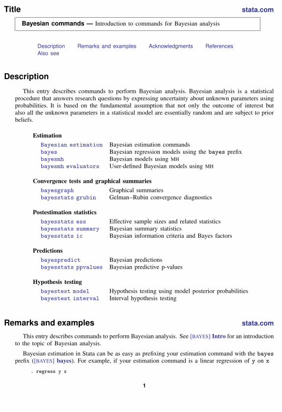
Description

This entry describes commands to perform Bayesian analysis. Bayesian analysis is a statisticalprocedure that answers research questions by expressing uncertainty about unknown parameters usingprobabilities. It is based on the fundamental assumption that not only the outcome of interest butalso all the unknown parameters in a statistical model are essentially random and are subject to priorbeliefs.

EstimationBayesian estimation Bayesian estimation commandsbayes Bayesian regression models using the bayes prefixbayesmh Bayesian models using MHbayesmh evaluators User-defined Bayesian models using MH

Convergence tests and graphical summariesbayesgraph Graphical summariesbayesstats grubin Gelman–Rubin convergence diagnostics

Postestimation statisticsbayesstats ess Effective sample sizes and related statisticsbayesstats summary Bayesian summary statisticsbayesstats ic Bayesian information criteria and Bayes factors

Predictionsbayespredict Bayesian predictionsbayesstats ppvalues Bayesian predictive p-values

Hypothesis testingbayestest model Hypothesis testing using model posterior probabilitiesbayestest interval Interval hypothesis testing

Remarks and examples stata.com

This entry describes commands to perform Bayesian analysis. See [BAYES] Intro for an introductionto the topic of Bayesian analysis.

Bayesian estimation in Stata can be as easy as prefixing your estimation command with the bayesprefix ([BAYES] bayes). For example, if your estimation command is a linear regression of y on x

. regress y x

1

2 Bayesian commands — Introduction to commands for Bayesian analysis

then Bayesian estimates for this model can be obtained by typing

. bayes: regress y x

See [BAYES] Bayesian estimation for a list of estimation commands that work with the bayesprefix.

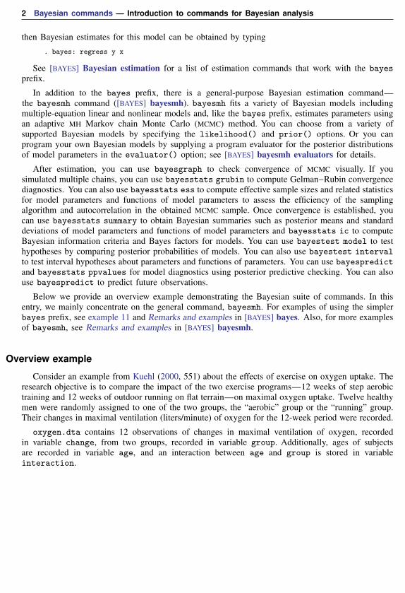
In addition to the bayes prefix, there is a general-purpose Bayesian estimation command—the bayesmh command ([BAYES] bayesmh). bayesmh fits a variety of Bayesian models includingmultiple-equation linear and nonlinear models and, like the bayes prefix, estimates parameters usingan adaptive MH Markov chain Monte Carlo (MCMC) method. You can choose from a variety ofsupported Bayesian models by specifying the likelihood() and prior() options. Or you canprogram your own Bayesian models by supplying a program evaluator for the posterior distributionsof model parameters in the evaluator() option; see [BAYES] bayesmh evaluators for details.

After estimation, you can use bayesgraph to check convergence of MCMC visually. If yousimulated multiple chains, you can use bayesstats grubin to compute Gelman–Rubin convergencediagnostics. You can also use bayesstats ess to compute effective sample sizes and related statisticsfor model parameters and functions of model parameters to assess the efficiency of the samplingalgorithm and autocorrelation in the obtained MCMC sample. Once convergence is established, youcan use bayesstats summary to obtain Bayesian summaries such as posterior means and standarddeviations of model parameters and functions of model parameters and bayesstats ic to computeBayesian information criteria and Bayes factors for models. You can use bayestest model to testhypotheses by comparing posterior probabilities of models. You can also use bayestest intervalto test interval hypotheses about parameters and functions of parameters. You can use bayespredictand bayesstats ppvalues for model diagnostics using posterior predictive checking. You can alsouse bayespredict to predict future observations.

Below we provide an overview example demonstrating the Bayesian suite of commands. In thisentry, we mainly concentrate on the general command, bayesmh. For examples of using the simplerbayes prefix, see example 11 and Remarks and examples in [BAYES] bayes. Also, for more examplesof bayesmh, see Remarks and examples in [BAYES] bayesmh.

Overview example

Consider an example from Kuehl (2000, 551) about the effects of exercise on oxygen uptake. Theresearch objective is to compare the impact of the two exercise programs—12 weeks of step aerobictraining and 12 weeks of outdoor running on flat terrain—on maximal oxygen uptake. Twelve healthymen were randomly assigned to one of the two groups, the “aerobic” group or the “running” group.Their changes in maximal ventilation (liters/minute) of oxygen for the 12-week period were recorded.

oxygen.dta contains 12 observations of changes in maximal ventilation of oxygen, recordedin variable change, from two groups, recorded in variable group. Additionally, ages of subjectsare recorded in variable age, and an interaction between age and group is stored in variableinteraction.

Bayesian commands — Introduction to commands for Bayesian analysis 3

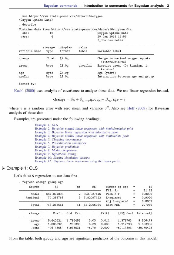
. use https://www.stata-press.com/data/r16/oxygen(Oxygen Uptake Data)

. describe

Contains data from https://www.stata-press.com/data/r16/oxygen.dtaobs: 12 Oxygen Uptake Data

vars: 4 20 Jan 2018 15:56(_dta has notes)

storage display valuevariable name type format label variable label

change float %9.0g Change in maximal oxygen uptake(liters/minute)

group byte %8.0g grouplab Exercise group (0: Running, 1:Aerobic)

age byte %8.0g Age (years)ageXgr byte %9.0g Interaction between age and group

Sorted by:

Kuehl (2000) uses analysis of covariance to analyze these data. We use linear regression instead,

change = β0 + βgroupgroup+ βageage+ ε

where ε is a random error with zero mean and variance σ2. Also see Hoff (2009) for Bayesiananalysis of these data.

Examples are presented under the following headings:

Example 1: OLSExample 2: Bayesian normal linear regression with noninformative priorExample 3: Bayesian linear regression with informative priorExample 4: Bayesian normal linear regression with multivariate priorExample 5: Checking convergenceExample 6: Postestimation summariesExample 7: Bayesian predictionsExample 8: Model comparisonExample 9: Hypothesis testingExample 10: Erasing simulation datasetsExample 11: Bayesian linear regression using the bayes prefix

Example 1: OLS

Let’s fit OLS regression to our data first.

. regress change group age

Source SS df MS Number of obs = 12F(2, 9) = 41.42

Model 647.874893 2 323.937446 Prob > F = 0.0000Residual 70.388768 9 7.82097423 R-squared = 0.9020

Adj R-squared = 0.8802Total 718.263661 11 65.2966964 Root MSE = 2.7966

change Coef. Std. Err. t P>|t| [95% Conf. Interval]

group 5.442621 1.796453 3.03 0.014 1.378763 9.506479age 1.885892 .295335 6.39 0.000 1.217798 2.553986

_cons -46.4565 6.936531 -6.70 0.000 -62.14803 -30.76498

From the table, both group and age are significant predictors of the outcome in this model.

4 Bayesian commands — Introduction to commands for Bayesian analysis

For example, we reject the hypothesis of H0: βgroup = 0 at a 5% level based on the p-value of0.014. The actual interpretation of the reported p-value is that if we repeat the same experiment anduse the same testing procedure many times, then given our null hypothesis of no effect of group, wewill observe the result (test statistic) as extreme or more extreme than the one observed in this sample(t = 3.03) only 1.4% of the times. The p-value cannot be interpreted as a probability of the nullhypothesis, which is a common misinterpretation. In fact, it answers the question of how likely ourdata are, given that the null hypothesis is true, and not how likely the null hypothesis is, given ourdata. The latter question can be answered using Bayesian hypothesis testing, which we demonstratein example 9.

Confidence intervals are popular alternatives to p-values that eliminate some of the p-valueshortcomings. For example, the 95% confidence interval for the coefficient for group is [1.38, 9.51]and does not contain the value of 0, so we consider group to be a significant predictor of change.The interpretation of a 95% confidence interval is that if we repeat the same experiment many timesand compute confidence intervals for each experiment, then 95% of those intervals will contain thetrue value of the parameter. Thus we cannot conclude that the true coefficient for group lies between1.38 and 9.51 with a probability of 0.95—a common misinterpretation of a confidence interval. Thisprobability is either 0 or 1, and we do not know which for any particular confidence interval. All weknow is that [1.38, 9.51] is a plausible range for the true value of the coefficient for group. Intervalsthat can actually be interpreted as probabilistic ranges for a parameter of interest may be constructedwithin the Bayesian paradigm; see example 9.

Example 2: Bayesian normal linear regression with noninformative prior

In example 1, we stated that frequentist methods cannot provide probabilistic summaries for theparameters of interest. This is because in frequentist statistics, parameters are viewed as unknown butfixed quantities. The only random quantity in a frequentist model is an outcome of interest. Bayesianstatistics, on the other hand, in addition to the outcome of interest, also treats all model parameters asrandom quantities. This is what sets Bayesian statistics apart from frequentist statistics and enablesone to make probability statements about the likely values of parameters and to assign probabilitiesto hypotheses of interest.

Bayesian statistics focuses on the estimation of various aspects of the posterior distribution of aparameter of interest, an initial or a prior distribution that has been updated with information abouta parameter contained in the observed data. A posterior distribution is thus described by the priordistribution of a parameter and the likelihood function of the data given the parameter.

Let’s now fit a Bayesian linear regression to oxygen.dta. To fit a Bayesian parametric model,we need to specify the likelihood function or the distribution of the data and prior distributions for allmodel parameters. Our Bayesian linear model has four parameters: three regression coefficients andthe variance of the data. We assume a normal distribution for our outcome, change, and start with anoninformative Jeffreys prior for the parameters. Under the Jeffreys prior, the joint prior distributionof the coefficients and the variance is proportional to the inverse of the variance.

We can write our model as follows,

change ∼ N(Xβ, σ2)

(β, σ2) ∼ 1

σ2

where X is our design matrix, and β = (β0, βgroup, βage)′, which is a vector of coefficients.

Bayesian commands — Introduction to commands for Bayesian analysis 5

We use the bayesmh command to fit our Bayesian model. Let’s consider the specification of themodel first.

bayesmh change group age, likelihood(normal({var})) ///prior({change:}, flat) prior({var}, jeffreys)

The specification of the regression function in bayesmh is the same as in any other Stata regressioncommand—the name of the dependent variable follows the command, and the covariates of interestare specified next. Likelihood or outcome distribution is specified in the likelihood() option, andprior distributions are specified in the prior() options, which are repeated options.

All model parameters must be specified in curly braces, {}. bayesmh automatically createsparameters associated with the regression function—regression coefficients—but it is your responsibilityto define the remaining model parameters. In our example, the only parameter we need to define is thevariance parameter, which we define as {var}. The three regression coefficients {change:group},{change:age}, and {change: cons} are automatically created by bayesmh.

The last step is to specify the likelihood and the prior distributions. bayesmh provides severaldifferent built-in distributions for the likelihood and priors. If a certain distribution is not available oryou have a particularly complicated Bayesian model, you may consider writing your own evaluatorfor the posterior distribution; see [BAYES] bayesmh evaluators for details. In our example, we specifydistribution normal({var}) in option likelihood() to request the likelihood function of the normalmodel with the variance parameter {var}. This specification together with the regression specificationdefines the likelihood model for our outcome change. We assign the flat prior, a prior with adensity of 1, to all regression coefficients with prior({change:}, flat), where {change:} isa shortcut for referring to all parameters with equation name change, our regression coefficients.Finally, we specify prior jeffreys for the variance parameter {var} to request the density 1/σ2.

Let’s now run our command. bayesmh uses MCMC sampling, specifically, an adaptive random-walkMH MCMC method, to estimate marginal posterior distributions of parameters. Because bayesmh isusing an MCMC method, which is stochastic, we must specify a random-number seed for reproducibilityof our results. For consistency and simplicity, we use the same random seed of 14 in all of ourexamples throughout the manual.

6 Bayesian commands — Introduction to commands for Bayesian analysis

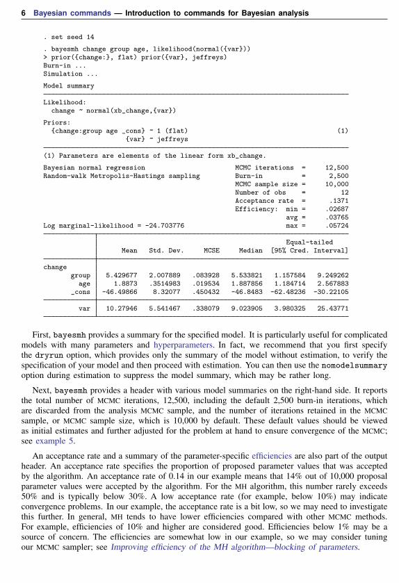
. set seed 14

. bayesmh change group age, likelihood(normal({var}))> prior({change:}, flat) prior({var}, jeffreys)Burn-in ...Simulation ...

Model summary

Likelihood:change ~ normal(xb_change,{var})

Priors:{change:group age _cons} ~ 1 (flat) (1)

{var} ~ jeffreys

(1) Parameters are elements of the linear form xb_change.

Bayesian normal regression MCMC iterations = 12,500Random-walk Metropolis-Hastings sampling Burn-in = 2,500

MCMC sample size = 10,000Number of obs = 12Acceptance rate = .1371Efficiency: min = .02687

avg = .03765Log marginal-likelihood = -24.703776 max = .05724

Equal-tailedMean Std. Dev. MCSE Median [95% Cred. Interval]

changegroup 5.429677 2.007889 .083928 5.533821 1.157584 9.249262

age 1.8873 .3514983 .019534 1.887856 1.184714 2.567883_cons -46.49866 8.32077 .450432 -46.8483 -62.48236 -30.22105

var 10.27946 5.541467 .338079 9.023905 3.980325 25.43771

First, bayesmh provides a summary for the specified model. It is particularly useful for complicatedmodels with many parameters and hyperparameters. In fact, we recommend that you first specifythe dryrun option, which provides only the summary of the model without estimation, to verify thespecification of your model and then proceed with estimation. You can then use the nomodelsummaryoption during estimation to suppress the model summary, which may be rather long.

Next, bayesmh provides a header with various model summaries on the right-hand side. It reportsthe total number of MCMC iterations, 12,500, including the default 2,500 burn-in iterations, whichare discarded from the analysis MCMC sample, and the number of iterations retained in the MCMCsample, or MCMC sample size, which is 10,000 by default. These default values should be viewedas initial estimates and further adjusted for the problem at hand to ensure convergence of the MCMC;see example 5.

An acceptance rate and a summary of the parameter-specific efficiencies are also part of the outputheader. An acceptance rate specifies the proportion of proposed parameter values that was acceptedby the algorithm. An acceptance rate of 0.14 in our example means that 14% out of 10,000 proposalparameter values were accepted by the algorithm. For the MH algorithm, this number rarely exceeds50% and is typically below 30%. A low acceptance rate (for example, below 10%) may indicateconvergence problems. In our example, the acceptance rate is a bit low, so we may need to investigatethis further. In general, MH tends to have lower efficiencies compared with other MCMC methods.For example, efficiencies of 10% and higher are considered good. Efficiencies below 1% may be asource of concern. The efficiencies are somewhat low in our example, so we may consider tuningour MCMC sampler; see Improving efficiency of the MH algorithm—blocking of parameters.

Bayesian commands — Introduction to commands for Bayesian analysis 7

Finally, bayesmh reports a table with a summary of the results. The Mean column reports theestimates of posterior means, which are means of the marginal posterior distributions of the parameters.The posterior mean estimates are pretty close to the OLS estimates obtained in example 1. This isexpected, provided MCMC converged, because we used a noninformative prior. That is, we did notprovide any additional information about parameters beyond that contained in the data.

The next column reports estimates of posterior standard deviations, which are standard deviationsof the marginal posterior distribution. These values describe the variability in the posterior distributionof the parameter and are comparable to our OLS standard errors.

The precision of the posterior mean estimates is described by their Monte Carlo standard errors.These numbers should be small, relative to the scales of the parameters. Increasing the MCMC samplesize should decrease these numbers.

The Median column provides estimates of the median of the posterior distribution and can be usedto assess the symmetries of the posterior distribution. At a quick glance, the estimates of posteriormeans and medians are pretty close for the regression coefficients, so we suspect that their posteriordistributions may be symmetric.

The last two columns provide credible intervals for the parameters. Unlike confidence intervals,as discussed in example 1, these intervals have a straightforward probabilistic interpretation. Forexample, the probability that the coefficient for group is between 1.16 and 9.25 is about 0.95. Thelower bound of the interval is greater than 0, so we conclude that there is an effect of the exerciseprogram on the change in oxygen uptake. We can also use Bayesian hypothesis testing to test effectsof parameters; see example 9.

Before any interpretation of the results, however, it is important to verify the convergence ofMCMC; see example 5.

See example 11 for how to fit Bayesian linear regression more easily using the bayes prefix.

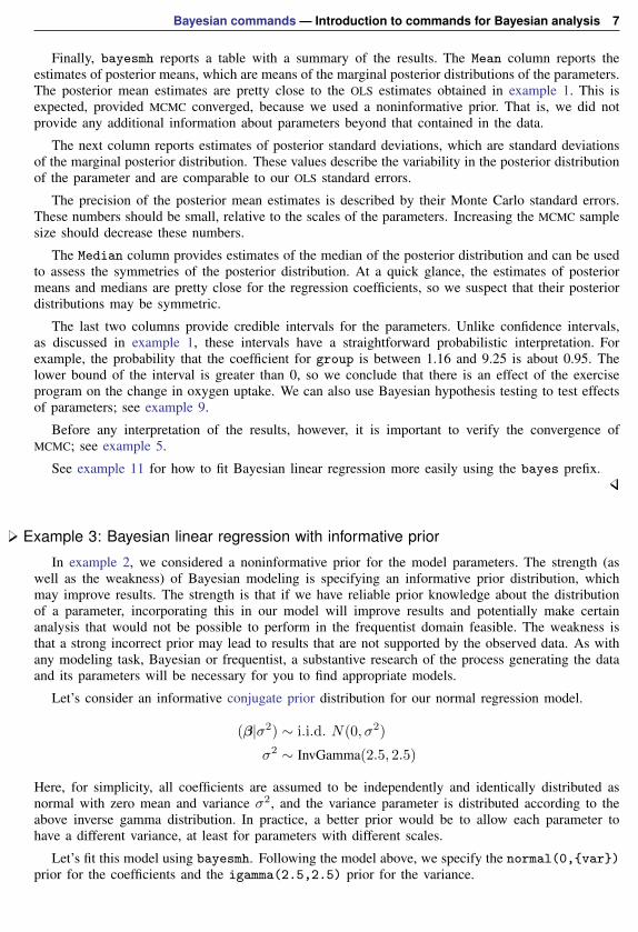
Example 3: Bayesian linear regression with informative prior

In example 2, we considered a noninformative prior for the model parameters. The strength (aswell as the weakness) of Bayesian modeling is specifying an informative prior distribution, whichmay improve results. The strength is that if we have reliable prior knowledge about the distributionof a parameter, incorporating this in our model will improve results and potentially make certainanalysis that would not be possible to perform in the frequentist domain feasible. The weakness isthat a strong incorrect prior may lead to results that are not supported by the observed data. As withany modeling task, Bayesian or frequentist, a substantive research of the process generating the dataand its parameters will be necessary for you to find appropriate models.

Let’s consider an informative conjugate prior distribution for our normal regression model.

(β|σ2) ∼ i.i.d. N(0, σ2)

σ2 ∼ InvGamma(2.5, 2.5)

Here, for simplicity, all coefficients are assumed to be independently and identically distributed asnormal with zero mean and variance σ2, and the variance parameter is distributed according to theabove inverse gamma distribution. In practice, a better prior would be to allow each parameter tohave a different variance, at least for parameters with different scales.

Let’s fit this model using bayesmh. Following the model above, we specify the normal(0,{var})prior for the coefficients and the igamma(2.5,2.5) prior for the variance.

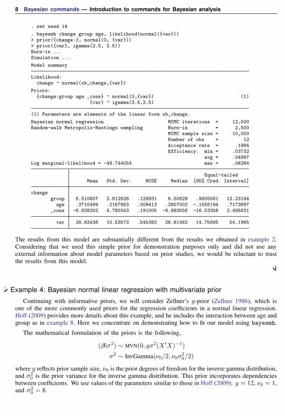
8 Bayesian commands — Introduction to commands for Bayesian analysis

. set seed 14

. bayesmh change group age, likelihood(normal({var}))> prior({change:}, normal(0, {var}))> prior({var}, igamma(2.5, 2.5))Burn-in ...Simulation ...

Model summary

Likelihood:change ~ normal(xb_change,{var})

Priors:{change:group age _cons} ~ normal(0,{var}) (1)

{var} ~ igamma(2.5,2.5)

(1) Parameters are elements of the linear form xb_change.

Bayesian normal regression MCMC iterations = 12,500Random-walk Metropolis-Hastings sampling Burn-in = 2,500

MCMC sample size = 10,000Number of obs = 12Acceptance rate = .1984Efficiency: min = .03732

avg = .04997Log marginal-likelihood = -49.744054 max = .06264

Equal-tailedMean Std. Dev. MCSE Median [95% Cred. Interval]

changegroup 6.510807 2.812828 .129931 6.50829 .9605561 12.23164

age .2710499 .2167863 .009413 .2657002 -.1556194 .7173697_cons -6.838302 4.780343 .191005 -6.683556 -16.53356 2.495631

var 28.83438 10.53573 .545382 26.81462 14.75695 54.1965

The results from this model are substantially different from the results we obtained in example 2.Considering that we used this simple prior for demonstration purposes only and did not use anyexternal information about model parameters based on prior studies, we would be reluctant to trustthe results from this model.

Example 4: Bayesian normal linear regression with multivariate prior

Continuing with informative priors, we will consider Zellner’s g-prior (Zellner 1986), which isone of the more commonly used priors for the regression coefficients in a normal linear regression.Hoff (2009) provides more details about this example, and he includes the interaction between age andgroup as in example 8. Here we concentrate on demonstrating how to fit our model using bayesmh.

The mathematical formulation of the priors is the following,

(β|σ2) ∼ MVN(0, gσ2(X ′X)−1)

σ2 ∼ InvGamma(ν0/2, ν0σ20/2)

where g reflects prior sample size, ν0 is the prior degrees of freedom for the inverse gamma distribution,and σ2

0 is the prior variance for the inverse gamma distribution. This prior incorporates dependenciesbetween coefficients. We use values of the parameters similar to those in Hoff (2009): g = 12, ν0 = 1,and σ2

0 = 8.

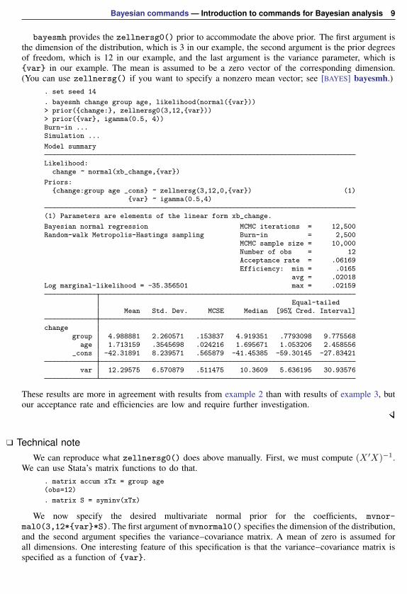
Bayesian commands — Introduction to commands for Bayesian analysis 9

bayesmh provides the zellnersg0() prior to accommodate the above prior. The first argument isthe dimension of the distribution, which is 3 in our example, the second argument is the prior degreesof freedom, which is 12 in our example, and the last argument is the variance parameter, which is{var} in our example. The mean is assumed to be a zero vector of the corresponding dimension.(You can use zellnersg() if you want to specify a nonzero mean vector; see [BAYES] bayesmh.)

. set seed 14

. bayesmh change group age, likelihood(normal({var}))> prior({change:}, zellnersg0(3,12,{var}))> prior({var}, igamma(0.5, 4))Burn-in ...Simulation ...

Model summary

Likelihood:change ~ normal(xb_change,{var})

Priors:{change:group age _cons} ~ zellnersg(3,12,0,{var}) (1)

{var} ~ igamma(0.5,4)

(1) Parameters are elements of the linear form xb_change.

Bayesian normal regression MCMC iterations = 12,500Random-walk Metropolis-Hastings sampling Burn-in = 2,500

MCMC sample size = 10,000Number of obs = 12Acceptance rate = .06169Efficiency: min = .0165

avg = .02018Log marginal-likelihood = -35.356501 max = .02159

Equal-tailedMean Std. Dev. MCSE Median [95% Cred. Interval]

changegroup 4.988881 2.260571 .153837 4.919351 .7793098 9.775568

age 1.713159 .3545698 .024216 1.695671 1.053206 2.458556_cons -42.31891 8.239571 .565879 -41.45385 -59.30145 -27.83421

var 12.29575 6.570879 .511475 10.3609 5.636195 30.93576

These results are more in agreement with results from example 2 than with results of example 3, butour acceptance rate and efficiencies are low and require further investigation.

Technical noteWe can reproduce what zellnersg0() does above manually. First, we must compute (X ′X)−1.

We can use Stata’s matrix functions to do that.. matrix accum xTx = group age(obs=12)

. matrix S = syminv(xTx)

We now specify the desired multivariate normal prior for the coefficients, mvnor-mal0(3,12*{var}*S). The first argument of mvnormal0() specifies the dimension of the distribution,and the second argument specifies the variance–covariance matrix. A mean of zero is assumed forall dimensions. One interesting feature of this specification is that the variance–covariance matrix isspecified as a function of {var}.

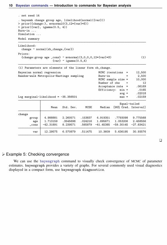
10 Bayesian commands — Introduction to commands for Bayesian analysis

. set seed 14

. bayesmh change group age, likelihood(normal({var}))> prior({change:}, mvnormal0(3,12*{var}*S))> prior({var}, igamma(0.5, 4))Burn-in ...Simulation ...

Model summary

Likelihood:change ~ normal(xb_change,{var})

Priors:{change:group age _cons} ~ mvnormal(3,0,0,0,12*{var}*S) (1)

{var} ~ igamma(0.5,4)

(1) Parameters are elements of the linear form xb_change.

Bayesian normal regression MCMC iterations = 12,500Random-walk Metropolis-Hastings sampling Burn-in = 2,500

MCMC sample size = 10,000Number of obs = 12Acceptance rate = .06169Efficiency: min = .0165

avg = .02018Log marginal-likelihood = -35.356501 max = .02159

Equal-tailedMean Std. Dev. MCSE Median [95% Cred. Interval]

changegroup 4.988881 2.260571 .153837 4.919351 .7793098 9.775568

age 1.713159 .3545698 .024216 1.695671 1.053206 2.458556_cons -42.31891 8.239571 .565879 -41.45385 -59.30145 -27.83421

var 12.29575 6.570879 .511475 10.3609 5.636195 30.93576

Example 5: Checking convergence

We can use the bayesgraph command to visually check convergence of MCMC of parameterestimates. bayesgraph provides a variety of graphs. For several commonly used visual diagnosticsdisplayed in a compact form, use bayesgraph diagnostics.

Bayesian commands — Introduction to commands for Bayesian analysis 11

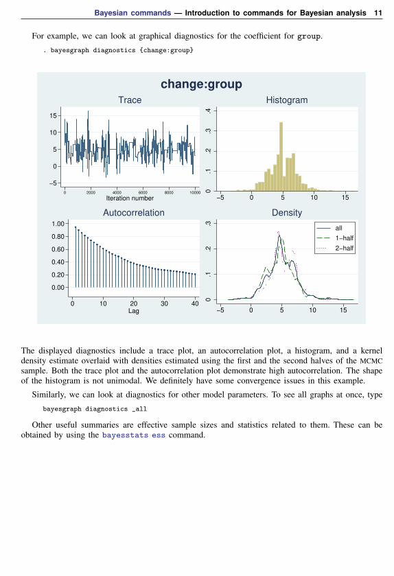
For example, we can look at graphical diagnostics for the coefficient for group.

. bayesgraph diagnostics {change:group}

−5

0

5

10

15

0 2000 4000 6000 8000 10000

Iteration number

Trace

0.1

.2.3

.4

−5 0 5 10 15

Histogram

0.00

0.20

0.40

0.60

0.80

1.00

0 10 20 30 40Lag

Autocorrelation0

.1.2

.3

−5 0 5 10 15

all

1−half

2−half

Density

change:group

The displayed diagnostics include a trace plot, an autocorrelation plot, a histogram, and a kerneldensity estimate overlaid with densities estimated using the first and the second halves of the MCMCsample. Both the trace plot and the autocorrelation plot demonstrate high autocorrelation. The shapeof the histogram is not unimodal. We definitely have some convergence issues in this example.

Similarly, we can look at diagnostics for other model parameters. To see all graphs at once, type

bayesgraph diagnostics _all

Other useful summaries are effective sample sizes and statistics related to them. These can beobtained by using the bayesstats ess command.

12 Bayesian commands — Introduction to commands for Bayesian analysis

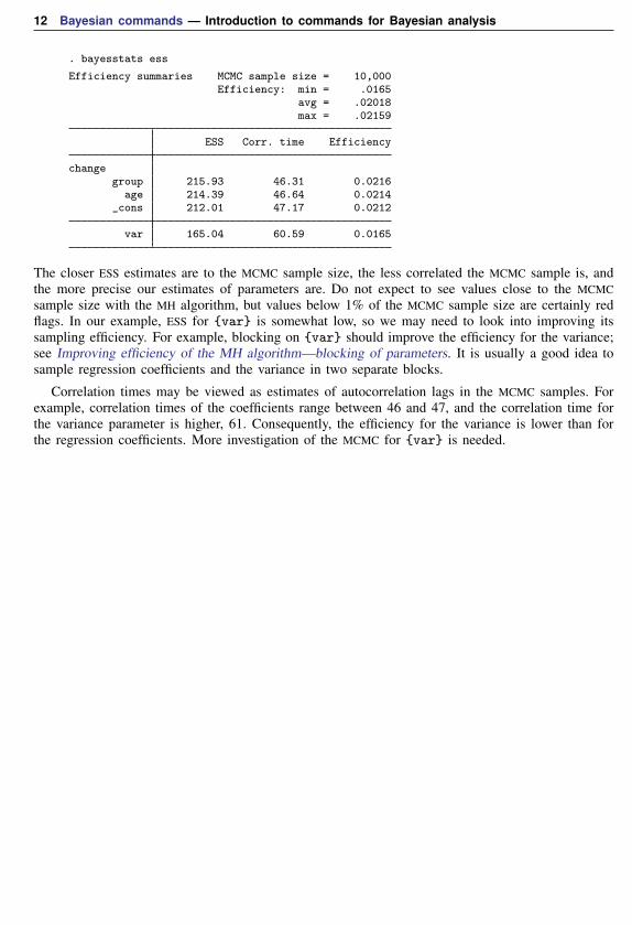
. bayesstats ess

Efficiency summaries MCMC sample size = 10,000Efficiency: min = .0165

avg = .02018max = .02159

ESS Corr. time Efficiency

changegroup 215.93 46.31 0.0216

age 214.39 46.64 0.0214_cons 212.01 47.17 0.0212

var 165.04 60.59 0.0165

The closer ESS estimates are to the MCMC sample size, the less correlated the MCMC sample is, andthe more precise our estimates of parameters are. Do not expect to see values close to the MCMCsample size with the MH algorithm, but values below 1% of the MCMC sample size are certainly redflags. In our example, ESS for {var} is somewhat low, so we may need to look into improving itssampling efficiency. For example, blocking on {var} should improve the efficiency for the variance;see Improving efficiency of the MH algorithm—blocking of parameters. It is usually a good idea tosample regression coefficients and the variance in two separate blocks.

Correlation times may be viewed as estimates of autocorrelation lags in the MCMC samples. Forexample, correlation times of the coefficients range between 46 and 47, and the correlation time forthe variance parameter is higher, 61. Consequently, the efficiency for the variance is lower than forthe regression coefficients. More investigation of the MCMC for {var} is needed.

Bayesian commands — Introduction to commands for Bayesian analysis 13

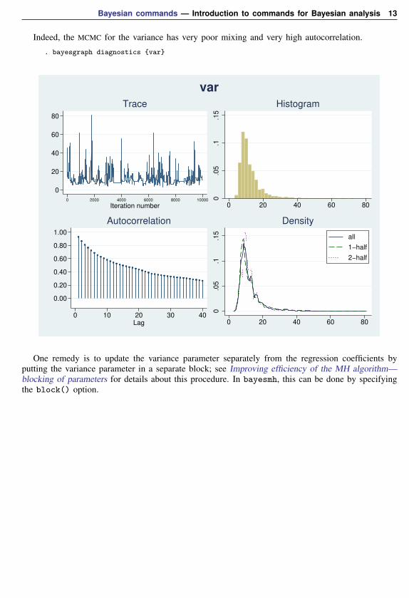
Indeed, the MCMC for the variance has very poor mixing and very high autocorrelation.

. bayesgraph diagnostics {var}

0

20

40

60

80

0 2000 4000 6000 8000 10000

Iteration number

Trace

0.0

5.1

.15

0 20 40 60 80

Histogram

0.00

0.20

0.40

0.60

0.80

1.00

0 10 20 30 40Lag

Autocorrelation0

.05

.1.1

5

0 20 40 60 80

all

1−half

2−half

Density

var

One remedy is to update the variance parameter separately from the regression coefficients byputting the variance parameter in a separate block; see Improving efficiency of the MH algorithm—blocking of parameters for details about this procedure. In bayesmh, this can be done by specifyingthe block() option.

14 Bayesian commands — Introduction to commands for Bayesian analysis

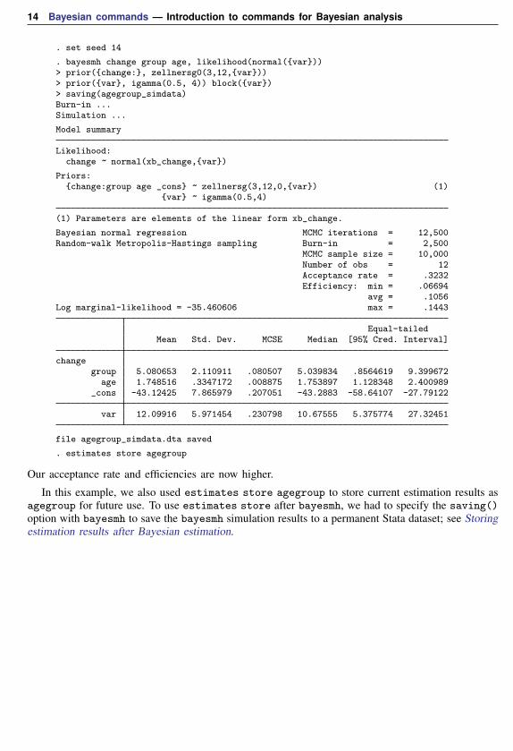
. set seed 14

. bayesmh change group age, likelihood(normal({var}))> prior({change:}, zellnersg0(3,12,{var}))> prior({var}, igamma(0.5, 4)) block({var})> saving(agegroup_simdata)Burn-in ...Simulation ...

Model summary

Likelihood:change ~ normal(xb_change,{var})

Priors:{change:group age _cons} ~ zellnersg(3,12,0,{var}) (1)

{var} ~ igamma(0.5,4)

(1) Parameters are elements of the linear form xb_change.

Bayesian normal regression MCMC iterations = 12,500Random-walk Metropolis-Hastings sampling Burn-in = 2,500

MCMC sample size = 10,000Number of obs = 12Acceptance rate = .3232Efficiency: min = .06694

avg = .1056Log marginal-likelihood = -35.460606 max = .1443

Equal-tailedMean Std. Dev. MCSE Median [95% Cred. Interval]

changegroup 5.080653 2.110911 .080507 5.039834 .8564619 9.399672

age 1.748516 .3347172 .008875 1.753897 1.128348 2.400989_cons -43.12425 7.865979 .207051 -43.2883 -58.64107 -27.79122

var 12.09916 5.971454 .230798 10.67555 5.375774 27.32451

file agegroup_simdata.dta saved

. estimates store agegroup

Our acceptance rate and efficiencies are now higher.

In this example, we also used estimates store agegroup to store current estimation results asagegroup for future use. To use estimates store after bayesmh, we had to specify the saving()option with bayesmh to save the bayesmh simulation results to a permanent Stata dataset; see Storingestimation results after Bayesian estimation.

Bayesian commands — Introduction to commands for Bayesian analysis 15

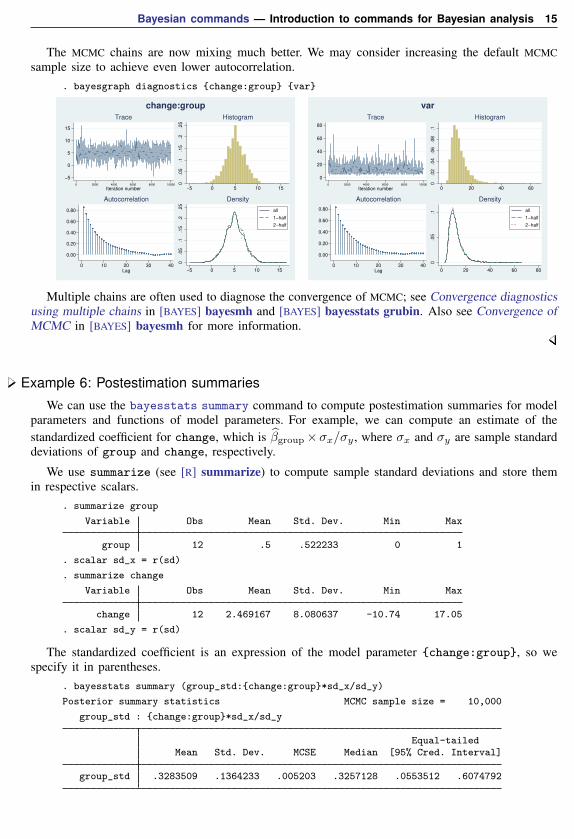
The MCMC chains are now mixing much better. We may consider increasing the default MCMCsample size to achieve even lower autocorrelation.

. bayesgraph diagnostics {change:group} {var}

−5

0

5

10

15

0 2000 4000 6000 8000 10000

Iteration number

Trace

0.0

5.1

.15

.2.2

5

−5 0 5 10 15

Histogram

0.00

0.20

0.40

0.60

0.80

0 10 20 30 40Lag

Autocorrelation

0.0

5.1

.15

.2.2

5

−5 0 5 10 15

all

1−half

2−half

Density

change:group

0

20

40

60

80

0 2000 4000 6000 8000 10000

Iteration number

Trace

0.0

2.0

4.0

6.0

8.1

0 20 40 60

Histogram

0.00

0.20

0.40

0.60

0.80

0 10 20 30 40Lag

Autocorrelation

0.0

5.1

0 20 40 60 80

all

1−half

2−half

Density

var

Multiple chains are often used to diagnose the convergence of MCMC; see Convergence diagnosticsusing multiple chains in [BAYES] bayesmh and [BAYES] bayesstats grubin. Also see Convergence ofMCMC in [BAYES] bayesmh for more information.

Example 6: Postestimation summaries

We can use the bayesstats summary command to compute postestimation summaries for modelparameters and functions of model parameters. For example, we can compute an estimate of thestandardized coefficient for change, which is β̂group×σx/σy , where σx and σy are sample standarddeviations of group and change, respectively.

We use summarize (see [R] summarize) to compute sample standard deviations and store themin respective scalars.

. summarize group

Variable Obs Mean Std. Dev. Min Max

group 12 .5 .522233 0 1

. scalar sd_x = r(sd)

. summarize change

Variable Obs Mean Std. Dev. Min Max

change 12 2.469167 8.080637 -10.74 17.05

. scalar sd_y = r(sd)

The standardized coefficient is an expression of the model parameter {change:group}, so wespecify it in parentheses.

. bayesstats summary (group_std:{change:group}*sd_x/sd_y)

Posterior summary statistics MCMC sample size = 10,000

group_std : {change:group}*sd_x/sd_y

Equal-tailedMean Std. Dev. MCSE Median [95% Cred. Interval]

group_std .3283509 .1364233 .005203 .3257128 .0553512 .6074792

16 Bayesian commands — Introduction to commands for Bayesian analysis

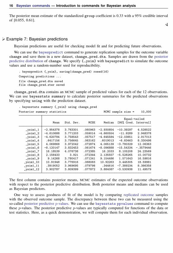
The posterior mean estimate of the standardized group coefficient is 0.33 with a 95% credible intervalof [0.055, 0.61].

Example 7: Bayesian predictions

Bayesian predictions are useful for checking model fit and for predicting future observations.

We can use the bayespredict command to generate replication samples for the outcome variablechange and save them in a new dataset, change pred.dta. Samples are drawn from the posteriorpredictive distribution of change. We specify { ysim} with bayespredict to simulate the outcomevalues and use a random-number seed for reproducibility.

. bayespredict {_ysim}, saving(change_pred) rseed(16)

Computing predictions ...

file change_pred.dta savedfile change_pred.ster saved

change pred.dta contains an MCMC sample of predicted values for each of the 12 observations.We can use bayesstats summary to calculate posterior summaries for the predicted observationsby specifying using with the prediction dataset.

. bayesstats summary {_ysim} using change_pred

Posterior summary statistics MCMC sample size = 10,000

Equal-tailedMean Std. Dev. MCSE Median [95% Cred. Interval]

_ysim1_1 -2.954378 3.763301 .060963 -2.930854 -10.39297 4.528522_ysim1_2 -4.610688 3.771203 .059014 -4.660554 -11.9289 2.948378_ysim1_3 -4.620784 3.758543 .057517 -4.645584 -12.03851 2.917013_ysim1_4 .6417156 3.756645 .063162 .6019013 -6.83463 8.330498_ysim1_5 4.069868 3.972042 .072874 4.065139 -3.780329 12.06363_ysim1_6 -8.120147 3.832453 .061674 -8.096888 -15.54334 -.3579446_ysim1_7 16.18539 4.076738 .072385 16.2033 8.105208 24.23569_ysim1_8 2.156433 3.921 .072344 2.135557 -5.528265 10.00732_ysim1_9 9.14268 3.780417 .071241 9.154486 1.571643 16.59816

_ysim1_10 10.91948 3.776916 .068083 10.92263 3.445305 18.59981_ysim1_11 .3919052 3.969695 .079798 .344616 -7.389234 8.386358_ysim1_12 3.902787 3.809399 .077872 3.884087 -3.530938 11.49579

The first column contains posterior means, MCMC estimates of the expected outcome observationswith respect to the posterior predictive distribution. Both posterior means and medians can be usedas Bayesian predictors.

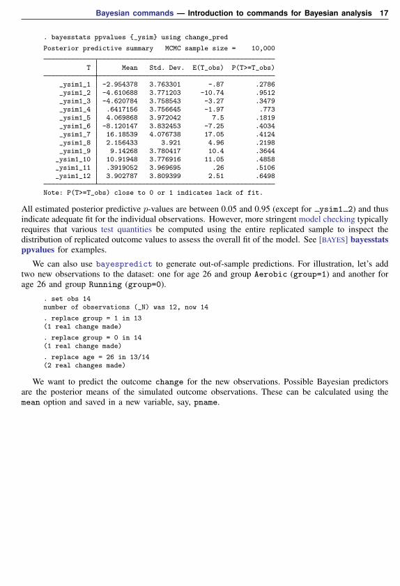
One way to assess goodness of fit of the model is by comparing replicated outcome sampleswith the observed outcome sample. The discrepancy between these two can be measured using theso-called posterior predictive p-values. We can use the bayesstats ppvalues command to computethese p-values. The posterior predictive p-values are typically computed for functions of the data ortest statistics. Here, as a quick demonstration, we will compute them for each individual observation.

Bayesian commands — Introduction to commands for Bayesian analysis 17

. bayesstats ppvalues {_ysim} using change_pred

Posterior predictive summary MCMC sample size = 10,000

T Mean Std. Dev. E(T_obs) P(T>=T_obs)

_ysim1_1 -2.954378 3.763301 -.87 .2786_ysim1_2 -4.610688 3.771203 -10.74 .9512_ysim1_3 -4.620784 3.758543 -3.27 .3479_ysim1_4 .6417156 3.756645 -1.97 .773_ysim1_5 4.069868 3.972042 7.5 .1819_ysim1_6 -8.120147 3.832453 -7.25 .4034_ysim1_7 16.18539 4.076738 17.05 .4124_ysim1_8 2.156433 3.921 4.96 .2198_ysim1_9 9.14268 3.780417 10.4 .3644

_ysim1_10 10.91948 3.776916 11.05 .4858_ysim1_11 .3919052 3.969695 .26 .5106_ysim1_12 3.902787 3.809399 2.51 .6498

Note: P(T>=T_obs) close to 0 or 1 indicates lack of fit.

All estimated posterior predictive p-values are between 0.05 and 0.95 (except for ysim1 2) and thusindicate adequate fit for the individual observations. However, more stringent model checking typicallyrequires that various test quantities be computed using the entire replicated sample to inspect thedistribution of replicated outcome values to assess the overall fit of the model. See [BAYES] bayesstatsppvalues for examples.

We can also use bayespredict to generate out-of-sample predictions. For illustration, let’s addtwo new observations to the dataset: one for age 26 and group Aerobic (group=1) and another forage 26 and group Running (group=0).

. set obs 14number of observations (_N) was 12, now 14

. replace group = 1 in 13(1 real change made)

. replace group = 0 in 14(1 real change made)

. replace age = 26 in 13/14(2 real changes made)

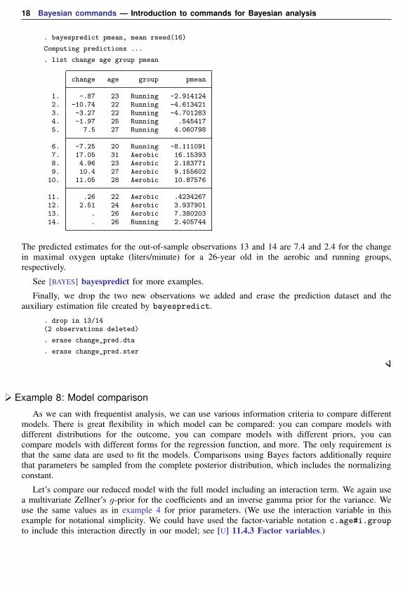
We want to predict the outcome change for the new observations. Possible Bayesian predictorsare the posterior means of the simulated outcome observations. These can be calculated using themean option and saved in a new variable, say, pname.

18 Bayesian commands — Introduction to commands for Bayesian analysis

. bayespredict pmean, mean rseed(16)

Computing predictions ...

. list change age group pmean

change age group pmean

1. -.87 23 Running -2.9141242. -10.74 22 Running -4.6134213. -3.27 22 Running -4.7012834. -1.97 25 Running .5454175. 7.5 27 Running 4.060798

6. -7.25 20 Running -8.1110917. 17.05 31 Aerobic 16.153938. 4.96 23 Aerobic 2.1837719. 10.4 27 Aerobic 9.155602

10. 11.05 28 Aerobic 10.87576

11. .26 22 Aerobic .423426712. 2.51 24 Aerobic 3.93790113. . 26 Aerobic 7.38020314. . 26 Running 2.405744

The predicted estimates for the out-of-sample observations 13 and 14 are 7.4 and 2.4 for the changein maximal oxygen uptake (liters/minute) for a 26-year old in the aerobic and running groups,respectively.

See [BAYES] bayespredict for more examples.

Finally, we drop the two new observations we added and erase the prediction dataset and theauxiliary estimation file created by bayespredict.

. drop in 13/14(2 observations deleted)

. erase change_pred.dta

. erase change_pred.ster

Example 8: Model comparison

As we can with frequentist analysis, we can use various information criteria to compare differentmodels. There is great flexibility in which model can be compared: you can compare models withdifferent distributions for the outcome, you can compare models with different priors, you cancompare models with different forms for the regression function, and more. The only requirement isthat the same data are used to fit the models. Comparisons using Bayes factors additionally requirethat parameters be sampled from the complete posterior distribution, which includes the normalizingconstant.

Let’s compare our reduced model with the full model including an interaction term. We again usea multivariate Zellner’s g-prior for the coefficients and an inverse gamma prior for the variance. Weuse the same values as in example 4 for prior parameters. (We use the interaction variable in thisexample for notational simplicity. We could have used the factor-variable notation c.age#i.groupto include this interaction directly in our model; see [U] 11.4.3 Factor variables.)

Bayesian commands — Introduction to commands for Bayesian analysis 19

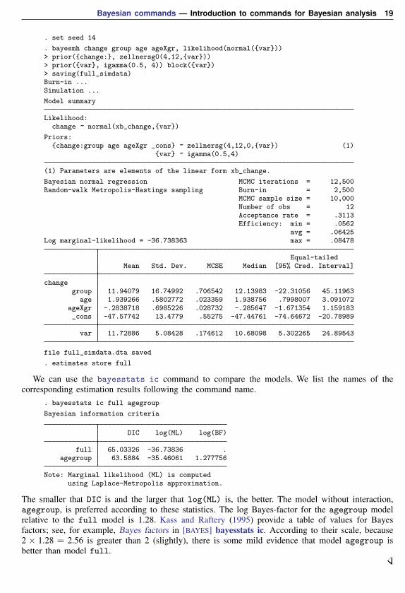
. set seed 14

. bayesmh change group age ageXgr, likelihood(normal({var}))> prior({change:}, zellnersg0(4,12,{var}))> prior({var}, igamma(0.5, 4)) block({var})> saving(full_simdata)Burn-in ...Simulation ...

Model summary

Likelihood:change ~ normal(xb_change,{var})

Priors:{change:group age ageXgr _cons} ~ zellnersg(4,12,0,{var}) (1)

{var} ~ igamma(0.5,4)

(1) Parameters are elements of the linear form xb_change.

Bayesian normal regression MCMC iterations = 12,500Random-walk Metropolis-Hastings sampling Burn-in = 2,500

MCMC sample size = 10,000Number of obs = 12Acceptance rate = .3113Efficiency: min = .0562

avg = .06425Log marginal-likelihood = -36.738363 max = .08478

Equal-tailedMean Std. Dev. MCSE Median [95% Cred. Interval]

changegroup 11.94079 16.74992 .706542 12.13983 -22.31056 45.11963

age 1.939266 .5802772 .023359 1.938756 .7998007 3.091072ageXgr -.2838718 .6985226 .028732 -.285647 -1.671354 1.159183_cons -47.57742 13.4779 .55275 -47.44761 -74.64672 -20.78989

var 11.72886 5.08428 .174612 10.68098 5.302265 24.89543

file full_simdata.dta saved

. estimates store full

We can use the bayesstats ic command to compare the models. We list the names of thecorresponding estimation results following the command name.

. bayesstats ic full agegroup

Bayesian information criteria

DIC log(ML) log(BF)

full 65.03326 -36.73836 .agegroup 63.5884 -35.46061 1.277756

Note: Marginal likelihood (ML) is computedusing Laplace-Metropolis approximation.

The smaller that DIC is and the larger that log(ML) is, the better. The model without interaction,agegroup, is preferred according to these statistics. The log Bayes-factor for the agegroup modelrelative to the full model is 1.28. Kass and Raftery (1995) provide a table of values for Bayesfactors; see, for example, Bayes factors in [BAYES] bayesstats ic. According to their scale, because2 × 1.28 = 2.56 is greater than 2 (slightly), there is some mild evidence that model agegroup isbetter than model full.

20 Bayesian commands — Introduction to commands for Bayesian analysis

Example 9: Hypothesis testing

Continuing with example 8, we can compute the actual probability associated with each of themodels. We can use the bayestest model command to do this.

Similar to bayesstats ic, this command requires the names of estimation results correspondingto the models of interest.

. bayestest model full agegroup

Bayesian model tests

log(ML) P(M) P(M|y)

full -36.7384 0.5000 0.2179agegroup -35.4606 0.5000 0.7821

Note: Marginal likelihood (ML) is computed usingLaplace-Metropolis approximation.

Under the assumption that both models are equally probable a priori, the model without interaction,agegroup, has the probability of 0.78, whereas the full model has the probability of only 0.22.Despite the drastic disparity in the probabilities, according to the results from example 8, modelagegroup is only slightly preferable to model full. To have stronger evidence against full, wewould expect to see higher probabilities (above 0.9) for agegroup.

We may be interested in testing an interval hypothesis about the parameter of interest. For example,for a model without interaction, let’s compute the probability that the coefficient for group is between4 and 8. We use estimates restore (see [R] estimates store) to load the results of the agegroupmodel back into memory.

. estimates restore agegroup(results agegroup are active now)

. bayestest interval {change:group}, lower(4) upper(8)

Interval tests MCMC sample size = 10,000

prob1 : 4 < {change:group} < 8

Mean Std. Dev. MCSE

prob1 .6159 0.48641 .0155788

The estimated probability or, technically, its posterior mean estimate is 0.62 with a standard deviationof 0.49 and Monte Carlo standard errors of 0.016.

Example 10: Erasing simulation datasets

After you are done with your analysis, remember to erase any simulation datasets that you createdusing bayesmh and no longer need. If you want to save your estimation results to disk for futurereference, use estimates save; see [R] estimates save.

We are done with our analysis, and we do not need the datasets for future reference, so we removeboth simulation files we created using bayesmh.

. erase agegroup_simdata.dta

. erase full_simdata.dta

Bayesian commands — Introduction to commands for Bayesian analysis 21

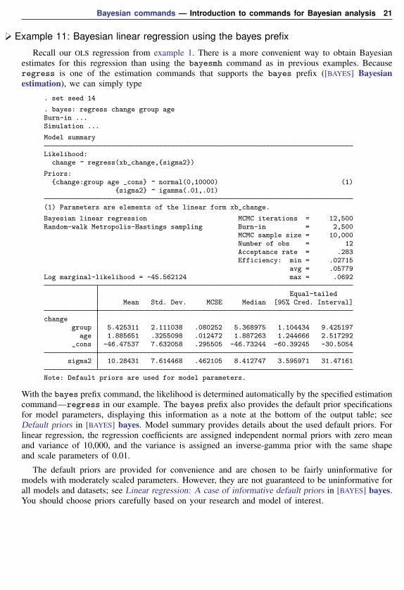
Example 11: Bayesian linear regression using the bayes prefix

Recall our OLS regression from example 1. There is a more convenient way to obtain Bayesianestimates for this regression than using the bayesmh command as in previous examples. Becauseregress is one of the estimation commands that supports the bayes prefix ([BAYES] Bayesianestimation), we can simply type

. set seed 14

. bayes: regress change group ageBurn-in ...Simulation ...

Model summary

Likelihood:change ~ regress(xb_change,{sigma2})

Priors:{change:group age _cons} ~ normal(0,10000) (1)

{sigma2} ~ igamma(.01,.01)

(1) Parameters are elements of the linear form xb_change.

Bayesian linear regression MCMC iterations = 12,500Random-walk Metropolis-Hastings sampling Burn-in = 2,500

MCMC sample size = 10,000Number of obs = 12Acceptance rate = .283Efficiency: min = .02715

avg = .05779Log marginal-likelihood = -45.562124 max = .0692

Equal-tailedMean Std. Dev. MCSE Median [95% Cred. Interval]

changegroup 5.425311 2.111038 .080252 5.368975 1.104434 9.425197

age 1.885651 .3255098 .012472 1.887263 1.244666 2.517292_cons -46.47537 7.632058 .295505 -46.73244 -60.39245 -30.5054

sigma2 10.28431 7.614468 .462105 8.412747 3.595971 31.47161

Note: Default priors are used for model parameters.

With the bayes prefix command, the likelihood is determined automatically by the specified estimationcommand—regress in our example. The bayes prefix also provides the default prior specificationsfor model parameters, displaying this information as a note at the bottom of the output table; seeDefault priors in [BAYES] bayes. Model summary provides details about the used default priors. Forlinear regression, the regression coefficients are assigned independent normal priors with zero meanand variance of 10,000, and the variance is assigned an inverse-gamma prior with the same shapeand scale parameters of 0.01.

The default priors are provided for convenience and are chosen to be fairly uninformative formodels with moderately scaled parameters. However, they are not guaranteed to be uninformative forall models and datasets; see Linear regression: A case of informative default priors in [BAYES] bayes.You should choose priors carefully based on your research and model of interest.

22 Bayesian commands — Introduction to commands for Bayesian analysis

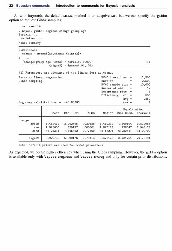
As with bayesmh, the default MCMC method is an adaptive MH, but we can specify the gibbsoption to request Gibbs sampling.

. set seed 14

. bayes, gibbs: regress change group ageBurn-in ...Simulation ...

Model summary

Likelihood:change ~ normal(xb_change,{sigma2})

Priors:{change:group age _cons} ~ normal(0,10000) (1)

{sigma2} ~ igamma(.01,.01)

(1) Parameters are elements of the linear form xb_change.

Bayesian linear regression MCMC iterations = 12,500Gibbs sampling Burn-in = 2,500

MCMC sample size = 10,000Number of obs = 12Acceptance rate = 1Efficiency: min = .556

avg = .889Log marginal-likelihood = -45.83666 max = 1

Equal-tailedMean Std. Dev. MCSE Median [95% Cred. Interval]

changegroup 5.452439 2.062795 .020628 5.460372 1.360104 9.512987

age 1.875606 .330127 .003301 1.877129 1.228647 2.543129_cons -46.21334 7.746862 .077469 -46.18291 -61.82541 -31.09702

sigma2 9.929756 5.899176 .079113 8.426173 3.731261 24.76194

Note: Default priors are used for model parameters.

As expected, we obtain higher efficiency when using the Gibbs sampling. However, the gibbs optionis available only with bayes: regress and bayes: mvreg and only for certain prior distributions.

Bayesian commands — Introduction to commands for Bayesian analysis 23

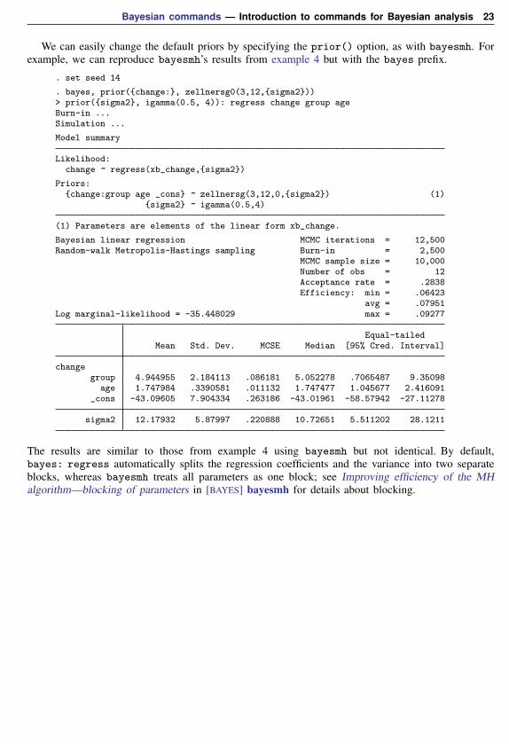
We can easily change the default priors by specifying the prior() option, as with bayesmh. Forexample, we can reproduce bayesmh’s results from example 4 but with the bayes prefix.

. set seed 14

. bayes, prior({change:}, zellnersg0(3,12,{sigma2}))> prior({sigma2}, igamma(0.5, 4)): regress change group ageBurn-in ...Simulation ...

Model summary

Likelihood:change ~ regress(xb_change,{sigma2})

Priors:{change:group age _cons} ~ zellnersg(3,12,0,{sigma2}) (1)

{sigma2} ~ igamma(0.5,4)

(1) Parameters are elements of the linear form xb_change.

Bayesian linear regression MCMC iterations = 12,500Random-walk Metropolis-Hastings sampling Burn-in = 2,500

MCMC sample size = 10,000Number of obs = 12Acceptance rate = .2838Efficiency: min = .06423

avg = .07951Log marginal-likelihood = -35.448029 max = .09277

Equal-tailedMean Std. Dev. MCSE Median [95% Cred. Interval]

changegroup 4.944955 2.184113 .086181 5.052278 .7065487 9.35098

age 1.747984 .3390581 .011132 1.747477 1.045677 2.416091_cons -43.09605 7.904334 .263186 -43.01961 -58.57942 -27.11278

sigma2 12.17932 5.87997 .220888 10.72651 5.511202 28.1211

The results are similar to those from example 4 using bayesmh but not identical. By default,bayes: regress automatically splits the regression coefficients and the variance into two separateblocks, whereas bayesmh treats all parameters as one block; see Improving efficiency of the MHalgorithm—blocking of parameters in [BAYES] bayesmh for details about blocking.

24 Bayesian commands — Introduction to commands for Bayesian analysis

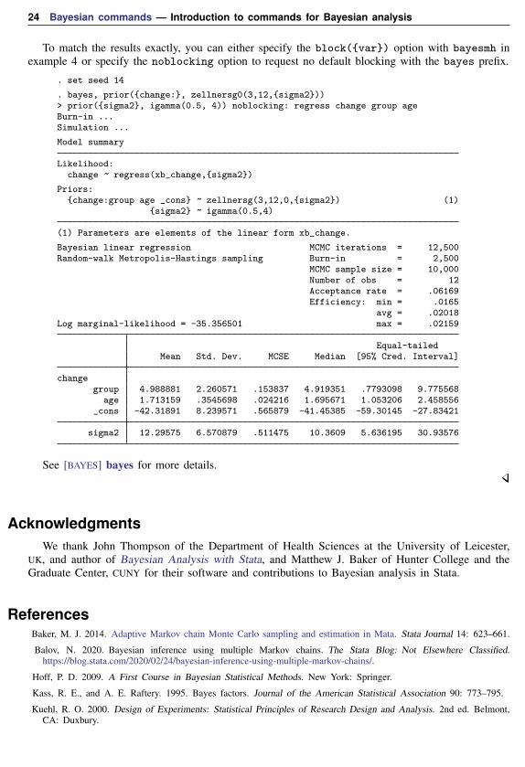
To match the results exactly, you can either specify the block({var}) option with bayesmh inexample 4 or specify the noblocking option to request no default blocking with the bayes prefix.

. set seed 14

. bayes, prior({change:}, zellnersg0(3,12,{sigma2}))> prior({sigma2}, igamma(0.5, 4)) noblocking: regress change group ageBurn-in ...Simulation ...

Model summary

Likelihood:change ~ regress(xb_change,{sigma2})

Priors:{change:group age _cons} ~ zellnersg(3,12,0,{sigma2}) (1)

{sigma2} ~ igamma(0.5,4)

(1) Parameters are elements of the linear form xb_change.

Bayesian linear regression MCMC iterations = 12,500Random-walk Metropolis-Hastings sampling Burn-in = 2,500

MCMC sample size = 10,000Number of obs = 12Acceptance rate = .06169Efficiency: min = .0165

avg = .02018Log marginal-likelihood = -35.356501 max = .02159

Equal-tailedMean Std. Dev. MCSE Median [95% Cred. Interval]

changegroup 4.988881 2.260571 .153837 4.919351 .7793098 9.775568

age 1.713159 .3545698 .024216 1.695671 1.053206 2.458556_cons -42.31891 8.239571 .565879 -41.45385 -59.30145 -27.83421

sigma2 12.29575 6.570879 .511475 10.3609 5.636195 30.93576

See [BAYES] bayes for more details.

AcknowledgmentsWe thank John Thompson of the Department of Health Sciences at the University of Leicester,

UK, and author of Bayesian Analysis with Stata, and Matthew J. Baker of Hunter College and theGraduate Center, CUNY for their software and contributions to Bayesian analysis in Stata.

ReferencesBaker, M. J. 2014. Adaptive Markov chain Monte Carlo sampling and estimation in Mata. Stata Journal 14: 623–661.

Balov, N. 2020. Bayesian inference using multiple Markov chains. The Stata Blog: Not Elsewhere Classified.https://blog.stata.com/2020/02/24/bayesian-inference-using-multiple-markov-chains/.

Hoff, P. D. 2009. A First Course in Bayesian Statistical Methods. New York: Springer.

Kass, R. E., and A. E. Raftery. 1995. Bayes factors. Journal of the American Statistical Association 90: 773–795.

Kuehl, R. O. 2000. Design of Experiments: Statistical Principles of Research Design and Analysis. 2nd ed. Belmont,CA: Duxbury.

Bayesian commands — Introduction to commands for Bayesian analysis 25

Zellner, A. 1986. On assessing prior distributions and Bayesian regression analysis with g-prior distributions. InVol. 6 of Bayesian Inference and Decision Techniques: Essays in Honor of Bruno De Finetti (Studies in BayesianEconometrics and Statistics), ed. P. K. Goel and A. Zellner, 233–343. Amsterdam: North-Holland.

Also see[BAYES] Intro — Introduction to Bayesian analysis

[BAYES] bayesmh — Bayesian models using Metropolis–Hastings algorithm

[BAYES] bayes — Bayesian regression models using the bayes prefix

[BAYES] Bayesian estimation — Bayesian estimation commands

[BAYES] Bayesian postestimation — Postestimation tools for bayesmh and the bayes prefix

[BAYES] Glossary