Thesis

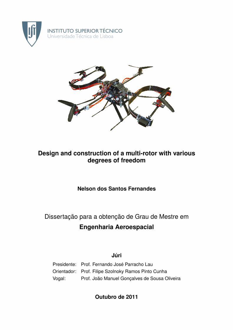
Design and construction of a multi-rotor with variousdegrees of freedom

Nelson dos Santos Fernandes

Dissertação para a obtenção de Grau de Mestre em

Engenharia Aeroespacial

Júri

Presidente: Prof. Fernando José Parracho LauOrientador: Prof. Filipe Szolnoky Ramos Pinto CunhaVogal: Prof. João Manuel Gonçalves de Sousa Oliveira

Outubro de 2011

ii

Aos meus pais e a minha irma.

iii

iv

Agradecimentos

Em primeiro lugar quero agradecer ao professor Filipe Cunha por todo o apoio, esclarecimentos,

ideias, alternativas e especialmente paciencia que teve ao longo de toda a tese.

Ao Engenheiro Severino Raposo, pela concecao do ALIV original e pela genese do conceito base

do quadrirotor com varios graus de liberdade. Ao Filipe Pedro pelo projeto preliminar que culminou na

presente tese e ao professor Agostinho Fonseca por toda a ajuda, ideias e material, indispensaveis

para o projeto.

Ao Alexandre Cruz pelas maos extra, na fase fulcral da construcao. Ao Andre Joao pelas dicas de

SolidWorks R©, ao Joao Domingos pelos grafismos profissionais, e a Helena Reis pelas dicas de ingles

mais que correto.

Ao Jose Vale e aos elementos seniores da S3A por toda a ajuda no laboratorio de Aeroespacial,

quer em pormenores quer em tecnicas de construcao, conceitos teoricos importantes ou apenas que

tornaram o trabalho no laboratorio mais leve.

Aos meus amigos e colegas que me aturaram e aturam e que de uma maneira ou de outra con-

tribuıram para a minha sanidade mental e por conseguinte para a conclusao deste projeto.

Por ultimo a minha famılia, em especial aos meus pais e a minha irma, por tudo, pois sem eles eu

nao seria.

v

vi

Resumo

Os quadrirotores sao uma das plataformas atualmente em maior desenvolvimento no mundo da

investigacao, devido a sua grande mobilidade, mas tambem ao seu potencial desenvolvimento como

aeronaves nao tripuladas capazes de pairar.

O objetivo deste projecto foi a construcao de uma aeronave de pequena dimensao, da fusao dos

conceitos de quadrirotor, com o de rotor inclinavel, possibilitando a sua movimentacao nos seis graus de

liberdade, com a vantagem de manter a sua zona central nivelada, independente da sua movimentacao

e velocidade, que possibilita ainda uma reducao do arrasto aerodinamico atraves da otimizacao da

superfıcie que enfrenta o escoamento. Esta possibilidade resulta da adicao de inclinacao em dois

rotores opostos em duas direcoes que nao a da sua rotacao.

Inicialmente foram exploradas algumas alternativas para o conceito de rotores inclinaveis e foram ex-

planadas as restantes componentes da aeronave. Tratando-se de um conceito de aeronave ainda inex-

plorado as suas capacidades de movimentacao foram totalmente determinadas. Um rotor otimo foi de-

senhado para a aeronave e todos os componentes necessarios para a sua construcao e implementacao

foram avaliados, selecionados ou desenhados e construıdos, sendo que a construcao foi feita em

compositos laminados. Por fim, analises de funcionamento dos atuadores, de performance em voo

e de arrasto aerodinamico foram efetuadas.

Esta tese contribuiu entao para a criacao desta plataforma inovadora para futuros trabalhos, espe-

cialmente plataformas de controlo, no contexto de quadrirotores com rotores de inclinacao variavel.

Palavras-chave: Quadrirotor, Rotores de inclinacao variavel, Compositos laminados, Rotor

otimo, ALIV3

vii

viii

Abstract

Quadrotors are currently one of the platforms under greater development in the academic world,

because of their great mobility but also the potential to develop unmanned aircrafts capable of hovering.

This project’s goal was to build a small-scale aircraft from the fusion of the quadrotor and tiltrotor

concepts, enabling it to move in all six degrees of freedom with the advantage of maintaining its central

core levelled, regardless of its movement and speed, which also allows a reduction in drag by optimizing

the surface facing the airflow. This possibility results from adding a tilting movement in two opposed

rotors in two directions, other than their rotation.

A few alternatives to the tilting rotors concept were explored, and the remaining components of

the aircraft were fully explained. Since this is an original aircraft concept, all its motion possibilities

were fully determined. An optimum rotor was designed for the aircraft and all the components needed

for its construction and implementation were evaluated, selected or designed and constructed. The

construction was done in laminated composites. Finally, analysis of servo’s operation, flight performance

and aerodynamic drag were conducted.

This thesis contributed to the creation of this innovative platform for future works, especially control

platforms, in the context of quadrotors with rotor tilting ability.

Keywords: Quadrotor, Tilting rotors, Laminated composites, Optimum rotor, ALIV3

ix

x

Contents

Agradecimentos . . . . . . . . . . . . . . . . . . . . . . . . . . . . . . . . . . . . . . . . . . . . v

Resumo . . . . . . . . . . . . . . . . . . . . . . . . . . . . . . . . . . . . . . . . . . . . . . . . . vii

Abstract . . . . . . . . . . . . . . . . . . . . . . . . . . . . . . . . . . . . . . . . . . . . . . . . . ix

List of Tables . . . . . . . . . . . . . . . . . . . . . . . . . . . . . . . . . . . . . . . . . . . . . . xvi

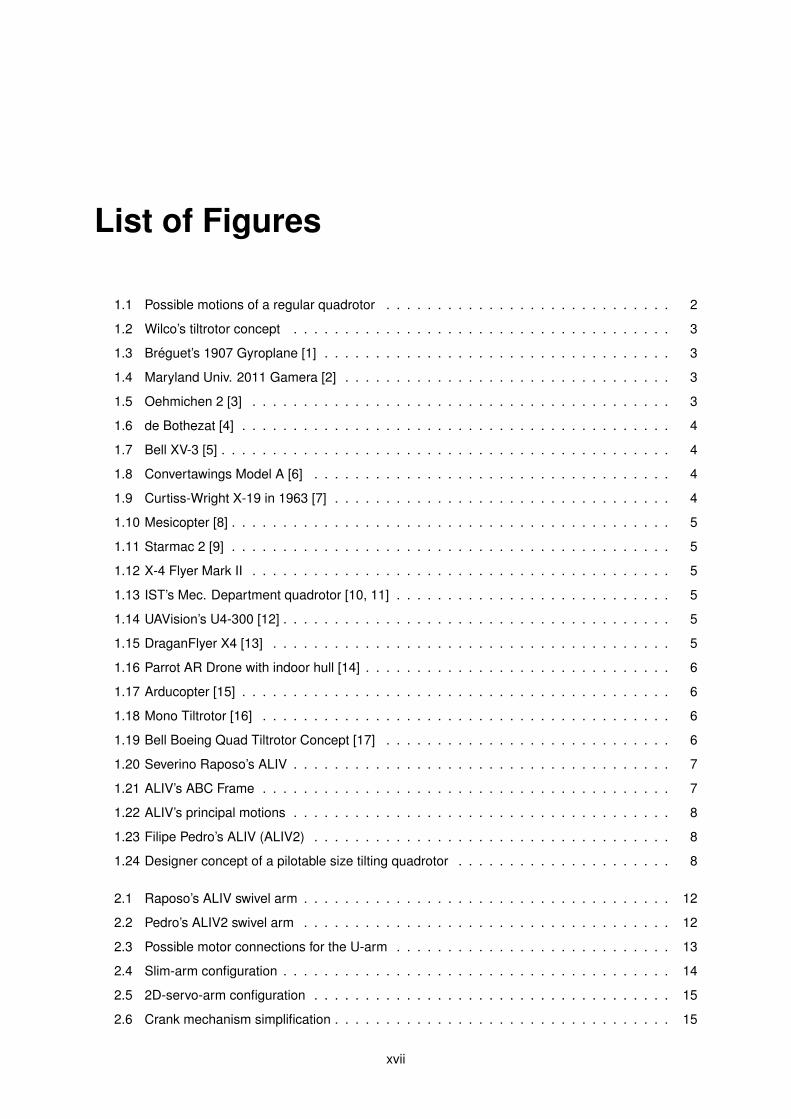
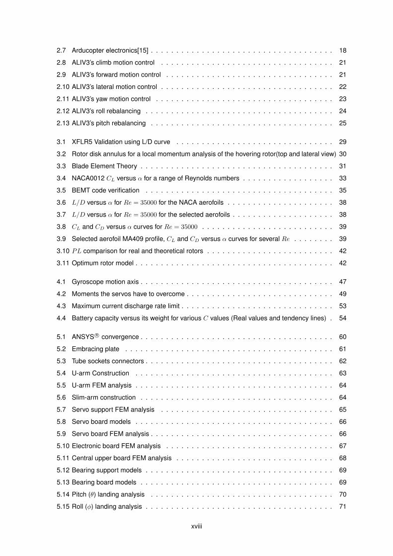
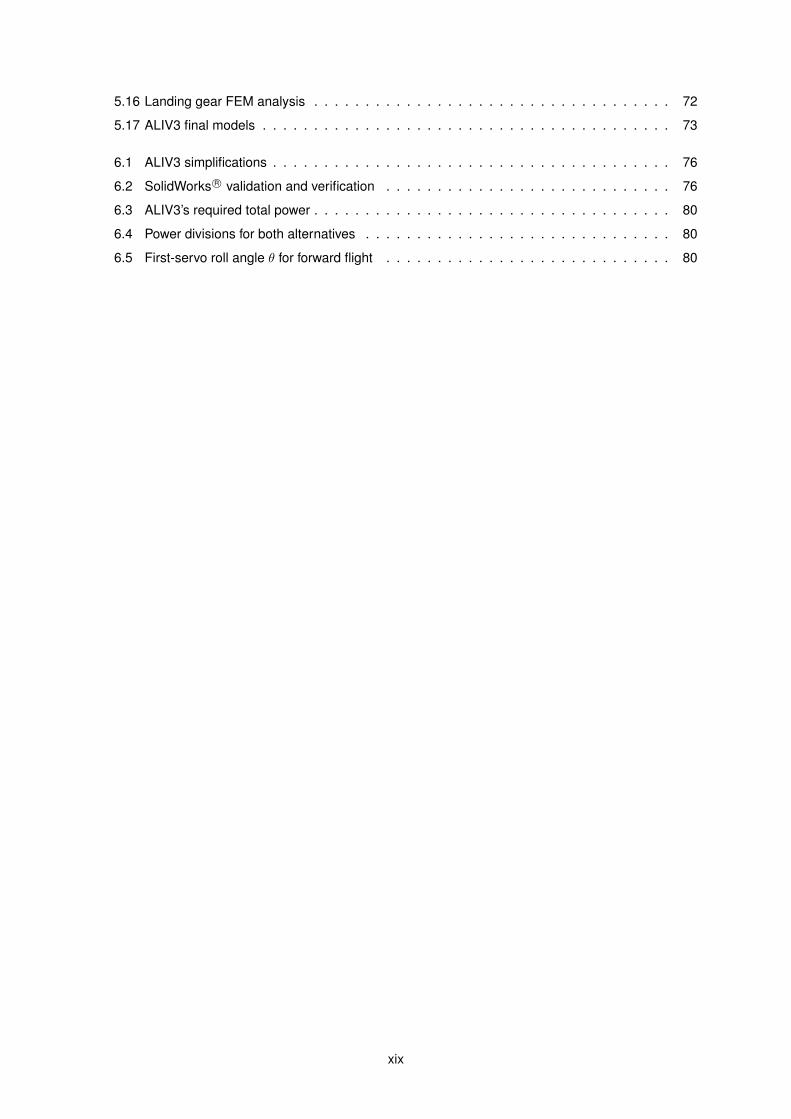
List of Figures . . . . . . . . . . . . . . . . . . . . . . . . . . . . . . . . . . . . . . . . . . . . . xix

Abbreviations and Acronyms . . . . . . . . . . . . . . . . . . . . . . . . . . . . . . . . . . . . . xxi

Nomenclature . . . . . . . . . . . . . . . . . . . . . . . . . . . . . . . . . . . . . . . . . . . . . . xxiii

1 Introduction 1

1.1 Concepts . . . . . . . . . . . . . . . . . . . . . . . . . . . . . . . . . . . . . . . . . . . . . 1

1.1.1 Quadrotor . . . . . . . . . . . . . . . . . . . . . . . . . . . . . . . . . . . . . . . . . 1

1.1.2 Tiltrotor . . . . . . . . . . . . . . . . . . . . . . . . . . . . . . . . . . . . . . . . . . 2

1.2 Historical Overview . . . . . . . . . . . . . . . . . . . . . . . . . . . . . . . . . . . . . . . . 2

1.3 State-of-the-art . . . . . . . . . . . . . . . . . . . . . . . . . . . . . . . . . . . . . . . . . . 4

1.3.1 Previous Work . . . . . . . . . . . . . . . . . . . . . . . . . . . . . . . . . . . . . . 6

1.4 Motivation . . . . . . . . . . . . . . . . . . . . . . . . . . . . . . . . . . . . . . . . . . . . . 9

1.5 Objective and Requisites . . . . . . . . . . . . . . . . . . . . . . . . . . . . . . . . . . . . 9

1.6 Thesis Structure . . . . . . . . . . . . . . . . . . . . . . . . . . . . . . . . . . . . . . . . . 10

2 Preliminary Design 11

2.1 Principal Structural Dimensions . . . . . . . . . . . . . . . . . . . . . . . . . . . . . . . . . 11

2.2 Swivel Arm Concept . . . . . . . . . . . . . . . . . . . . . . . . . . . . . . . . . . . . . . . 12

2.2.1 The U-arm . . . . . . . . . . . . . . . . . . . . . . . . . . . . . . . . . . . . . . . . 13

2.2.2 The Slim-arm . . . . . . . . . . . . . . . . . . . . . . . . . . . . . . . . . . . . . . . 14

2.2.3 The two-dimensional-servo-arm . . . . . . . . . . . . . . . . . . . . . . . . . . . . 15

2.2.4 Arm’s evaluation . . . . . . . . . . . . . . . . . . . . . . . . . . . . . . . . . . . . . 16

2.3 Central Area . . . . . . . . . . . . . . . . . . . . . . . . . . . . . . . . . . . . . . . . . . . 17

2.4 Landing Gear . . . . . . . . . . . . . . . . . . . . . . . . . . . . . . . . . . . . . . . . . . . 19

2.5 Motion Control . . . . . . . . . . . . . . . . . . . . . . . . . . . . . . . . . . . . . . . . . . 19

2.5.1 Levelled motions . . . . . . . . . . . . . . . . . . . . . . . . . . . . . . . . . . . . . 20

2.5.2 Rebalancing operations . . . . . . . . . . . . . . . . . . . . . . . . . . . . . . . . . 23

xi

2.5.3 Combined motions . . . . . . . . . . . . . . . . . . . . . . . . . . . . . . . . . . . . 26

3 Rotor Optimization 27

3.1 Theoretical principles . . . . . . . . . . . . . . . . . . . . . . . . . . . . . . . . . . . . . . 27

3.1.1 Panel Method . . . . . . . . . . . . . . . . . . . . . . . . . . . . . . . . . . . . . . . 27

3.1.2 Blade Element Momentum Theory . . . . . . . . . . . . . . . . . . . . . . . . . . . 30

3.1.3 Genetic Algorithm . . . . . . . . . . . . . . . . . . . . . . . . . . . . . . . . . . . . 36

3.2 Aerofoil selection . . . . . . . . . . . . . . . . . . . . . . . . . . . . . . . . . . . . . . . . . 38

3.3 Optimum rotor . . . . . . . . . . . . . . . . . . . . . . . . . . . . . . . . . . . . . . . . . . 40

4 Off-the-shelf Components 43

4.1 Propulsion Components . . . . . . . . . . . . . . . . . . . . . . . . . . . . . . . . . . . . . 43

4.2 Servos . . . . . . . . . . . . . . . . . . . . . . . . . . . . . . . . . . . . . . . . . . . . . . . 46

4.3 Avionics . . . . . . . . . . . . . . . . . . . . . . . . . . . . . . . . . . . . . . . . . . . . . . 49

4.4 Communication . . . . . . . . . . . . . . . . . . . . . . . . . . . . . . . . . . . . . . . . . . 51

4.5 Battery . . . . . . . . . . . . . . . . . . . . . . . . . . . . . . . . . . . . . . . . . . . . . . . 52

4.6 Structural Components . . . . . . . . . . . . . . . . . . . . . . . . . . . . . . . . . . . . . 55

4.7 Extra Components . . . . . . . . . . . . . . . . . . . . . . . . . . . . . . . . . . . . . . . . 56

5 Design and Construction 57

5.1 Theoretical principles . . . . . . . . . . . . . . . . . . . . . . . . . . . . . . . . . . . . . . 57

5.1.1 Laminated composites . . . . . . . . . . . . . . . . . . . . . . . . . . . . . . . . . . 57

5.1.2 Finite Element Method (FEM) . . . . . . . . . . . . . . . . . . . . . . . . . . . . . . 59

5.1.3 Laminated composite manufacturing process . . . . . . . . . . . . . . . . . . . . . 60

5.2 Structural project . . . . . . . . . . . . . . . . . . . . . . . . . . . . . . . . . . . . . . . . . 61

5.2.1 Fixed arm . . . . . . . . . . . . . . . . . . . . . . . . . . . . . . . . . . . . . . . . . 61

5.2.2 Swivel arm . . . . . . . . . . . . . . . . . . . . . . . . . . . . . . . . . . . . . . . . 62

5.2.3 Servo board . . . . . . . . . . . . . . . . . . . . . . . . . . . . . . . . . . . . . . . 65

5.2.4 Electronic board . . . . . . . . . . . . . . . . . . . . . . . . . . . . . . . . . . . . . 66

5.2.5 Central board and remaining central parts . . . . . . . . . . . . . . . . . . . . . . . 67

5.2.6 Landing gear . . . . . . . . . . . . . . . . . . . . . . . . . . . . . . . . . . . . . . . 70

5.3 Final design . . . . . . . . . . . . . . . . . . . . . . . . . . . . . . . . . . . . . . . . . . . . 72

6 Performance 75

6.1 Drag Analysis . . . . . . . . . . . . . . . . . . . . . . . . . . . . . . . . . . . . . . . . . . . 75

6.1.1 SolidWorks R© CFD analysis verification and validation . . . . . . . . . . . . . . . . 76

6.1.2 Flight drag analysis . . . . . . . . . . . . . . . . . . . . . . . . . . . . . . . . . . . 76

6.2 Servo testing . . . . . . . . . . . . . . . . . . . . . . . . . . . . . . . . . . . . . . . . . . . 77

6.3 Flight performance . . . . . . . . . . . . . . . . . . . . . . . . . . . . . . . . . . . . . . . . 78

xii

7 Conclusions 81

7.1 Future Work . . . . . . . . . . . . . . . . . . . . . . . . . . . . . . . . . . . . . . . . . . . . 82

Bibliography 86

A Centre of mass 87

A.1 ALIV . . . . . . . . . . . . . . . . . . . . . . . . . . . . . . . . . . . . . . . . . . . . . . . . 87

A.2 ALIV3 . . . . . . . . . . . . . . . . . . . . . . . . . . . . . . . . . . . . . . . . . . . . . . . 87

B BEMT.m 88

C GA.m 91

D Tested aerofoils 96

E Servo calculations 97

F Analytical determination for laminated composites displacement 98

G Detailed weight of every component 99

xiii

xiv

List of Tables

1.1 ALIV3 project requisits . . . . . . . . . . . . . . . . . . . . . . . . . . . . . . . . . . . . . . 10

2.1 Arm’s weighted decision matrix . . . . . . . . . . . . . . . . . . . . . . . . . . . . . . . . . 17

3.1 Reynolds related properties for small rotors . . . . . . . . . . . . . . . . . . . . . . . . . . 33

3.2 Testing rotors’ properties . . . . . . . . . . . . . . . . . . . . . . . . . . . . . . . . . . . . . 35

3.3 CT results comparison . . . . . . . . . . . . . . . . . . . . . . . . . . . . . . . . . . . . . . 35

3.4 CP results comparison . . . . . . . . . . . . . . . . . . . . . . . . . . . . . . . . . . . . . . 36

3.5 Small scale rotor’s results comparison . . . . . . . . . . . . . . . . . . . . . . . . . . . . . 36

3.6 BEMT properties . . . . . . . . . . . . . . . . . . . . . . . . . . . . . . . . . . . . . . . . . 40

3.7 Limits of the parameters to be estimated . . . . . . . . . . . . . . . . . . . . . . . . . . . . 41

3.8 Optimum rotor properties and results . . . . . . . . . . . . . . . . . . . . . . . . . . . . . . 41

4.1 Motor properties . . . . . . . . . . . . . . . . . . . . . . . . . . . . . . . . . . . . . . . . . 44

4.2 Selected motors test results . . . . . . . . . . . . . . . . . . . . . . . . . . . . . . . . . . . 45

4.3 ESC properties . . . . . . . . . . . . . . . . . . . . . . . . . . . . . . . . . . . . . . . . . . 46

4.4 Servo properties . . . . . . . . . . . . . . . . . . . . . . . . . . . . . . . . . . . . . . . . . 49

4.5 Avionic component properties . . . . . . . . . . . . . . . . . . . . . . . . . . . . . . . . . . 51

4.6 Communication component properties . . . . . . . . . . . . . . . . . . . . . . . . . . . . . 52

4.7 Battery properties . . . . . . . . . . . . . . . . . . . . . . . . . . . . . . . . . . . . . . . . 54

4.8 PDB properties . . . . . . . . . . . . . . . . . . . . . . . . . . . . . . . . . . . . . . . . . . 55

4.9 Material properties . . . . . . . . . . . . . . . . . . . . . . . . . . . . . . . . . . . . . . . . 55

4.10 Arm section determination . . . . . . . . . . . . . . . . . . . . . . . . . . . . . . . . . . . . 56

4.11 Camera properties . . . . . . . . . . . . . . . . . . . . . . . . . . . . . . . . . . . . . . . . 56

5.1 Composite elements properties . . . . . . . . . . . . . . . . . . . . . . . . . . . . . . . . . 58

5.2 Laminae properties . . . . . . . . . . . . . . . . . . . . . . . . . . . . . . . . . . . . . . . . 58

5.3 Validation of maximum displacement between ANSYS R© and the theoretic formulations . . 60

5.4 Thickness evaluation for the U-arm . . . . . . . . . . . . . . . . . . . . . . . . . . . . . . . 63

5.5 Thickness evaluation for the servo support . . . . . . . . . . . . . . . . . . . . . . . . . . . 64

5.6 Thickness evaluation for the servo board . . . . . . . . . . . . . . . . . . . . . . . . . . . . 66

5.7 Thickness evaluation for the electronic board . . . . . . . . . . . . . . . . . . . . . . . . . 67

xv

5.8 Thickness evaluation for the central boards . . . . . . . . . . . . . . . . . . . . . . . . . . 68

5.9 Thickness evaluation for the landing gear . . . . . . . . . . . . . . . . . . . . . . . . . . . 72

6.1 Drag analysis . . . . . . . . . . . . . . . . . . . . . . . . . . . . . . . . . . . . . . . . . . . 77

6.2 Servo testing . . . . . . . . . . . . . . . . . . . . . . . . . . . . . . . . . . . . . . . . . . . 78

E.1 Inertia and angular derivatives for maximum servo torque estimation . . . . . . . . . . . . 97

G.1 U-arm model detailed weight . . . . . . . . . . . . . . . . . . . . . . . . . . . . . . . . . . 99

G.2 Slim-arm model detailed weight . . . . . . . . . . . . . . . . . . . . . . . . . . . . . . . . . 100

xvi

List of Figures

1.1 Possible motions of a regular quadrotor . . . . . . . . . . . . . . . . . . . . . . . . . . . . 2

1.2 Wilco’s tiltrotor concept . . . . . . . . . . . . . . . . . . . . . . . . . . . . . . . . . . . . . 3

1.3 Breguet’s 1907 Gyroplane [1] . . . . . . . . . . . . . . . . . . . . . . . . . . . . . . . . . . 3

1.4 Maryland Univ. 2011 Gamera [2] . . . . . . . . . . . . . . . . . . . . . . . . . . . . . . . . 3

1.5 Oehmichen 2 [3] . . . . . . . . . . . . . . . . . . . . . . . . . . . . . . . . . . . . . . . . . 3

1.6 de Bothezat [4] . . . . . . . . . . . . . . . . . . . . . . . . . . . . . . . . . . . . . . . . . . 4

1.7 Bell XV-3 [5] . . . . . . . . . . . . . . . . . . . . . . . . . . . . . . . . . . . . . . . . . . . . 4

1.8 Convertawings Model A [6] . . . . . . . . . . . . . . . . . . . . . . . . . . . . . . . . . . . 4

1.9 Curtiss-Wright X-19 in 1963 [7] . . . . . . . . . . . . . . . . . . . . . . . . . . . . . . . . . 4

1.10 Mesicopter [8] . . . . . . . . . . . . . . . . . . . . . . . . . . . . . . . . . . . . . . . . . . . 5

1.11 Starmac 2 [9] . . . . . . . . . . . . . . . . . . . . . . . . . . . . . . . . . . . . . . . . . . . 5

1.12 X-4 Flyer Mark II . . . . . . . . . . . . . . . . . . . . . . . . . . . . . . . . . . . . . . . . . 5

1.13 IST’s Mec. Department quadrotor [10, 11] . . . . . . . . . . . . . . . . . . . . . . . . . . . 5

1.14 UAVision’s U4-300 [12] . . . . . . . . . . . . . . . . . . . . . . . . . . . . . . . . . . . . . . 5

1.15 DraganFlyer X4 [13] . . . . . . . . . . . . . . . . . . . . . . . . . . . . . . . . . . . . . . . 5

1.16 Parrot AR Drone with indoor hull [14] . . . . . . . . . . . . . . . . . . . . . . . . . . . . . . 6

1.17 Arducopter [15] . . . . . . . . . . . . . . . . . . . . . . . . . . . . . . . . . . . . . . . . . . 6

1.18 Mono Tiltrotor [16] . . . . . . . . . . . . . . . . . . . . . . . . . . . . . . . . . . . . . . . . 6

1.19 Bell Boeing Quad Tiltrotor Concept [17] . . . . . . . . . . . . . . . . . . . . . . . . . . . . 6

1.20 Severino Raposo’s ALIV . . . . . . . . . . . . . . . . . . . . . . . . . . . . . . . . . . . . . 7

1.21 ALIV’s ABC Frame . . . . . . . . . . . . . . . . . . . . . . . . . . . . . . . . . . . . . . . . 7

1.22 ALIV’s principal motions . . . . . . . . . . . . . . . . . . . . . . . . . . . . . . . . . . . . . 8

1.23 Filipe Pedro’s ALIV (ALIV2) . . . . . . . . . . . . . . . . . . . . . . . . . . . . . . . . . . . 8

1.24 Designer concept of a pilotable size tilting quadrotor . . . . . . . . . . . . . . . . . . . . . 8

2.1 Raposo’s ALIV swivel arm . . . . . . . . . . . . . . . . . . . . . . . . . . . . . . . . . . . . 12

2.2 Pedro’s ALIV2 swivel arm . . . . . . . . . . . . . . . . . . . . . . . . . . . . . . . . . . . . 12

2.3 Possible motor connections for the U-arm . . . . . . . . . . . . . . . . . . . . . . . . . . . 13

2.4 Slim-arm configuration . . . . . . . . . . . . . . . . . . . . . . . . . . . . . . . . . . . . . . 14

2.5 2D-servo-arm configuration . . . . . . . . . . . . . . . . . . . . . . . . . . . . . . . . . . . 15

2.6 Crank mechanism simplification . . . . . . . . . . . . . . . . . . . . . . . . . . . . . . . . . 15

xvii

2.7 Arducopter electronics[15] . . . . . . . . . . . . . . . . . . . . . . . . . . . . . . . . . . . . 18

2.8 ALIV3’s climb motion control . . . . . . . . . . . . . . . . . . . . . . . . . . . . . . . . . . 21

2.9 ALIV3’s forward motion control . . . . . . . . . . . . . . . . . . . . . . . . . . . . . . . . . 21

2.10 ALIV3’s lateral motion control . . . . . . . . . . . . . . . . . . . . . . . . . . . . . . . . . . 22

2.11 ALIV3’s yaw motion control . . . . . . . . . . . . . . . . . . . . . . . . . . . . . . . . . . . 23

2.12 ALIV3’s roll rebalancing . . . . . . . . . . . . . . . . . . . . . . . . . . . . . . . . . . . . . 24

2.13 ALIV3’s pitch rebalancing . . . . . . . . . . . . . . . . . . . . . . . . . . . . . . . . . . . . 25

3.1 XFLR5 Validation using L/D curve . . . . . . . . . . . . . . . . . . . . . . . . . . . . . . . 29

3.2 Rotor disk annulus for a local momentum analysis of the hovering rotor(top and lateral view) 30

3.3 Blade Element Theory . . . . . . . . . . . . . . . . . . . . . . . . . . . . . . . . . . . . . . 31

3.4 NACA0012 CL versus α for a range of Reynolds numbers . . . . . . . . . . . . . . . . . . 33

3.5 BEMT code verification . . . . . . . . . . . . . . . . . . . . . . . . . . . . . . . . . . . . . 35

3.6 L/D versus α for Re = 35000 for the NACA aerofoils . . . . . . . . . . . . . . . . . . . . . 38

3.7 L/D versus α for Re = 35000 for the selected aerofoils . . . . . . . . . . . . . . . . . . . . 38

3.8 CL and CD versus α curves for Re = 35000 . . . . . . . . . . . . . . . . . . . . . . . . . . 39

3.9 Selected aerofoil MA409 profile, CL and CD versus α curves for several Re . . . . . . . . 39

3.10 PL comparison for real and theoretical rotors . . . . . . . . . . . . . . . . . . . . . . . . . 42

3.11 Optimum rotor model . . . . . . . . . . . . . . . . . . . . . . . . . . . . . . . . . . . . . . . 42

4.1 Gyroscope motion axis . . . . . . . . . . . . . . . . . . . . . . . . . . . . . . . . . . . . . . 47

4.2 Moments the servos have to overcome . . . . . . . . . . . . . . . . . . . . . . . . . . . . . 49

4.3 Maximum current discharge rate limit . . . . . . . . . . . . . . . . . . . . . . . . . . . . . . 53

4.4 Battery capacity versus its weight for various C values (Real values and tendency lines) . 54

5.1 ANSYS R© convergence . . . . . . . . . . . . . . . . . . . . . . . . . . . . . . . . . . . . . . 60

5.2 Embracing plate . . . . . . . . . . . . . . . . . . . . . . . . . . . . . . . . . . . . . . . . . 61

5.3 Tube sockets connectors . . . . . . . . . . . . . . . . . . . . . . . . . . . . . . . . . . . . . 62

5.4 U-arm Construction . . . . . . . . . . . . . . . . . . . . . . . . . . . . . . . . . . . . . . . 63

5.5 U-arm FEM analysis . . . . . . . . . . . . . . . . . . . . . . . . . . . . . . . . . . . . . . . 64

5.6 Slim-arm construction . . . . . . . . . . . . . . . . . . . . . . . . . . . . . . . . . . . . . . 64

5.7 Servo support FEM analysis . . . . . . . . . . . . . . . . . . . . . . . . . . . . . . . . . . 65

5.8 Servo board models . . . . . . . . . . . . . . . . . . . . . . . . . . . . . . . . . . . . . . . 66

5.9 Servo board FEM analysis . . . . . . . . . . . . . . . . . . . . . . . . . . . . . . . . . . . . 66

5.10 Electronic board FEM analysis . . . . . . . . . . . . . . . . . . . . . . . . . . . . . . . . . 67

5.11 Central upper board FEM analysis . . . . . . . . . . . . . . . . . . . . . . . . . . . . . . . 68

5.12 Bearing support models . . . . . . . . . . . . . . . . . . . . . . . . . . . . . . . . . . . . . 69

5.13 Bearing board models . . . . . . . . . . . . . . . . . . . . . . . . . . . . . . . . . . . . . . 69

5.14 Pitch (θ) landing analysis . . . . . . . . . . . . . . . . . . . . . . . . . . . . . . . . . . . . 70

5.15 Roll (φ) landing analysis . . . . . . . . . . . . . . . . . . . . . . . . . . . . . . . . . . . . . 71

xviii

5.16 Landing gear FEM analysis . . . . . . . . . . . . . . . . . . . . . . . . . . . . . . . . . . . 72

5.17 ALIV3 final models . . . . . . . . . . . . . . . . . . . . . . . . . . . . . . . . . . . . . . . . 73

6.1 ALIV3 simplifications . . . . . . . . . . . . . . . . . . . . . . . . . . . . . . . . . . . . . . . 76

6.2 SolidWorks R© validation and verification . . . . . . . . . . . . . . . . . . . . . . . . . . . . 76

6.3 ALIV3’s required total power . . . . . . . . . . . . . . . . . . . . . . . . . . . . . . . . . . . 80

6.4 Power divisions for both alternatives . . . . . . . . . . . . . . . . . . . . . . . . . . . . . . 80

6.5 First-servo roll angle θ for forward flight . . . . . . . . . . . . . . . . . . . . . . . . . . . . 80

xix

xx

Abbreviations and Acronyms

ABC Aircraft-Body-Centred (frame, assumed as body fixed frame)

ALIV Autonomous Locomotion Individual Vehicle

BEMT Blade Element Momentum Theory

BET Blade Element Theory

CFD Computational Fluid Dynamics

CNC Computer Numerical Control

DC Direct Current

ESC Electronic Speed Control

FEM Finite Element Method

FVM Finite Volume Method

GA Genetic Algorithm

GPS Global Positioning System

HT High Tenacity

IST Instituto Superior Tecnico

LQR Linear Quadratic Regulator

MAV Micro Air Vehicle

NASA National Aeronautics and Space Administration

NED North East Down (inertial frame)

PDB Power Distribution Board

RC Radio Control

xxi

STOL Short Take-Off and Landing

UAV Unmanned Aerial Vehicle

VTOL Vertical Take-Off and Landing

xxii

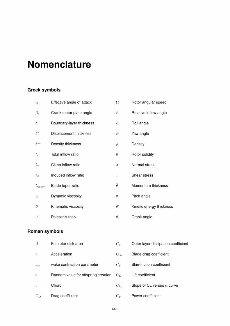
Nomenclature

Greek symbols

α Effective angle of attack Ω Rotor angular speed

βc Crank motor plate angle φ Relative inflow angle

δ Boundary-layer thickness φ Roll angle

δ∗ Displacement thickness ψ Yaw angle

δ∗∗ Density thickness ρ Density

λ Total inflow ratio σ Rotor solidity

λc Climb inflow ratio σ Normal stress

λi Induced inflow ratio τ Shear stress

λtaper Blade taper ratio θ Momentum thickness

µ Dynamic viscosity θ Pitch angle

ν Kinematic viscosity θ∗ Kinetic energy thickness

ν Poisson’s ratio θc Crank angle

Roman symbols

A Full rotor disk area Cd Outer layer dissipation coefficient

a Acceleration Cd0Blade drag coefficient

aw wake contraction parameter Cf Skin-friction coefficient

b Random value for offspring creation CL Lift coefficient

c Chord CLα Slope of CL versus α curve

CD Drag coefficient CP Power coefficient

xxiii

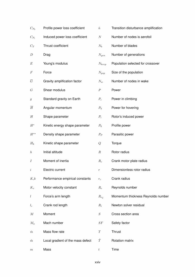
CP0 Profile power loss coefficient n Transition disturbance amplification

CPi Induced power loss coefficient N Number of nodes is aerofoil

CT Thrust coefficient Nb Number of blades

D Drag Ngen Number of generations

E Young’s modulus Nkeep Population selected for crossover

F Force Npop Size of the population

G Gravity amplification factor Nw Number of nodes in wake

G Shear modulus P Power

g Standard gravity on Earth Pc Power in climbing

H Angular momentum Ph Power for hovering

H Shape parameter Pi Rotor’s induced power

H∗ Kinetic energy shape parameter P0 Profile power

H∗∗ Density shape parameter PP Parasitic power

Hk Kinetic shape parameter Q Torque

h Initial altitude R Rotor radius

I Moment of inertia Rc Crank motor plate radius

i Electric current r Dimensionless rotor radius

K,k Performance empirical constants rc Crank radius

Kv Motor velocity constant Re Reynolds number

l Force’s arm length Reθ Momentum thickness Reynolds number

lc Crank rod length Ri Newton solver residual

M Moment S Cross section area

Ma Mach number SF Safety factor

m Mass flow rate T Thrust

m Local gradient of the mass defect T Rotation matrix

m Mass t Time

xxiv

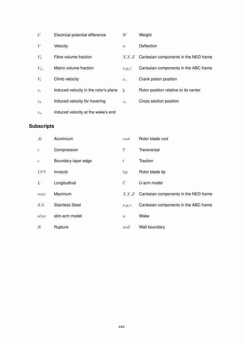
U Electrical potential difference W Weight

V Velocity w Deflection

Vf Fibre volume fraction X,Y ,Z Cartesian components in the NED frame

Vm Matrix volume fraction x,y,z Cartesian components in the ABC frame

Vc Climb velocity xc Crank piston position

vi Induced velocity in the rotor’s plane y Rotor position relative to its center

vh Induced velocity for hovering zs Cross section position

vw Induced velocity at the wake’s end

Subscripts

Al Aluminium root Rotor blade root

c Compression T Transversal

e Boundary-layer edge t Traction

INV Inviscid tip Rotor blade tip

L Longitudinal U U-arm model

max Maximum X,Y ,Z Cartesian components in the NED frame

S.S. Stainless Steel x,y,z Cartesian components in the ABC frame

slim slim-arm model w Wake

R Rupture wall Wall boundary

xxv

xxvi

Chapter 1

Introduction

The present Master’s dissertation arises in sequence of Filipe Pedro’s work [18] from 2009, in which

the author envisioned an upgraded version of Severino Raposo’s Autonomous Locomotion Individual

Vehicle (ALIV) [19], an unconventional quadrotor, able to manoeuvre in all the six degrees of freedom

such as the conventional quadrotor, adding the advantageous ability to maintain the central core of the

aircraft in a levelled position, independent of the aircraft’s movement and velocity, such improvement

resulting from the addition of a tilting movement in two opposed rotors in two directions, other than their

rotation.

1.1 Concepts

Firstly a few key concepts must be introduced, for a better understanding of the underlying idea

behind this project, such as the Quadrotor itself and the tilting mechanism of a motor-rotor couple.

1.1.1 Quadrotor

The principles of the quadrotor, also known as a quadrotor helicopter or even quadcopter, date back

to 1907 by the French Breguet brothers, with what they called ”Gyroplane” (figure 1.3), which according

to Leishman [20], ”carried a pilot off the ground, albeit briefly. [...] Clearly, the machine never flew

completely freely because [...] it lacked stability and a proper means of control”.

A quadrotor is an aircraft heavier than air, capable of vertical take-off and landing (VTOL), which is

propelled by four rotors, positioned in the same plane, parallel to the ground. Unlike standard helicopters,

a quadrotor uses fixed-pitch blades in its rotors and its motion through the air is achieved by varying the

relative speed of each propeller as is shown in figure 1.1. In a standard quadrotor, opposed rotors

turn in the same direction, rotors one and three turn clockwise whereas rotors two and four spin in a

counter-clockwise manner. This characteristic is mandatory so that the torque produced by each couple

is cancelled by the other pair, making the control of a quadrotor symmetric, and this aspect leads to the

necessity of absolute symmetry in a quadrotor, and the neutrality of its centre of mass, perfectly centred

in a plane parallel to the rotors’ plane.

1

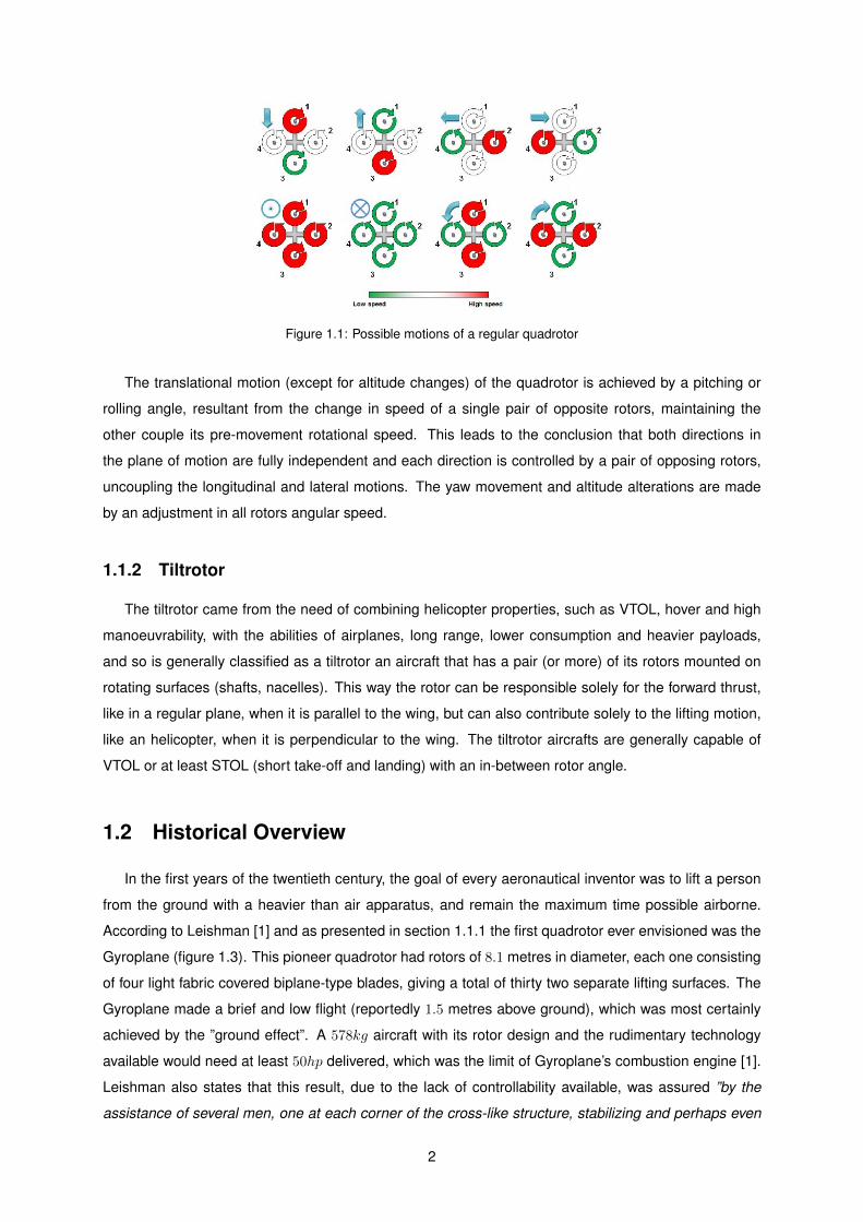
Figure 1.1: Possible motions of a regular quadrotor

The translational motion (except for altitude changes) of the quadrotor is achieved by a pitching or

rolling angle, resultant from the change in speed of a single pair of opposite rotors, maintaining the

other couple its pre-movement rotational speed. This leads to the conclusion that both directions in

the plane of motion are fully independent and each direction is controlled by a pair of opposing rotors,

uncoupling the longitudinal and lateral motions. The yaw movement and altitude alterations are made

by an adjustment in all rotors angular speed.

1.1.2 Tiltrotor

The tiltrotor came from the need of combining helicopter properties, such as VTOL, hover and high

manoeuvrability, with the abilities of airplanes, long range, lower consumption and heavier payloads,

and so is generally classified as a tiltrotor an aircraft that has a pair (or more) of its rotors mounted on

rotating surfaces (shafts, nacelles). This way the rotor can be responsible solely for the forward thrust,

like in a regular plane, when it is parallel to the wing, but can also contribute solely to the lifting motion,

like an helicopter, when it is perpendicular to the wing. The tiltrotor aircrafts are generally capable of

VTOL or at least STOL (short take-off and landing) with an in-between rotor angle.

1.2 Historical Overview

In the first years of the twentieth century, the goal of every aeronautical inventor was to lift a person

from the ground with a heavier than air apparatus, and remain the maximum time possible airborne.

According to Leishman [1] and as presented in section 1.1.1 the first quadrotor ever envisioned was the

Gyroplane (figure 1.3). This pioneer quadrotor had rotors of 8.1 metres in diameter, each one consisting

of four light fabric covered biplane-type blades, giving a total of thirty two separate lifting surfaces. The

Gyroplane made a brief and low flight (reportedly 1.5 metres above ground), which was most certainly

achieved by the ”ground effect”. A 578kg aircraft with its rotor design and the rudimentary technology

available would need at least 50hp delivered, which was the limit of Gyroplane’s combustion engine [1].

Leishman also states that this result, due to the lack of controllability available, was assured ”by the

assistance of several men, one at each corner of the cross-like structure, stabilizing and perhaps even

2

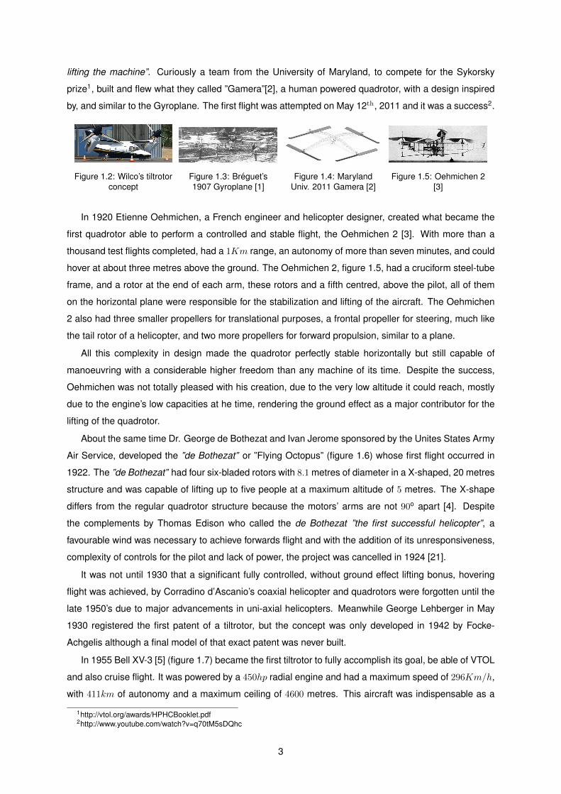
lifting the machine”. Curiously a team from the University of Maryland, to compete for the Sykorsky

prize1, built and flew what they called ”Gamera”[2], a human powered quadrotor, with a design inspired

by, and similar to the Gyroplane. The first flight was attempted on May 12th, 2011 and it was a success2.

Figure 1.2: Wilco’s tiltrotorconcept

Figure 1.3: Breguet’s1907 Gyroplane [1]

Figure 1.4: MarylandUniv. 2011 Gamera [2]

Figure 1.5: Oehmichen 2[3]

In 1920 Etienne Oehmichen, a French engineer and helicopter designer, created what became the

first quadrotor able to perform a controlled and stable flight, the Oehmichen 2 [3]. With more than a

thousand test flights completed, had a 1Km range, an autonomy of more than seven minutes, and could

hover at about three metres above the ground. The Oehmichen 2, figure 1.5, had a cruciform steel-tube

frame, and a rotor at the end of each arm, these rotors and a fifth centred, above the pilot, all of them

on the horizontal plane were responsible for the stabilization and lifting of the aircraft. The Oehmichen

2 also had three smaller propellers for translational purposes, a frontal propeller for steering, much like

the tail rotor of a helicopter, and two more propellers for forward propulsion, similar to a plane.

All this complexity in design made the quadrotor perfectly stable horizontally but still capable of

manoeuvring with a considerable higher freedom than any machine of its time. Despite the success,

Oehmichen was not totally pleased with his creation, due to the very low altitude it could reach, mostly

due to the engine’s low capacities at he time, rendering the ground effect as a major contributor for the

lifting of the quadrotor.

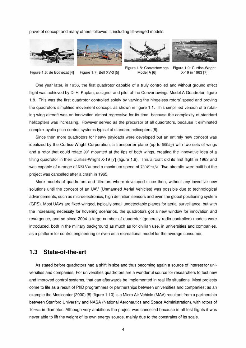
About the same time Dr. George de Bothezat and Ivan Jerome sponsored by the Unites States Army

Air Service, developed the ”de Bothezat” or ”Flying Octopus” (figure 1.6) whose first flight occurred in

1922. The ”de Bothezat” had four six-bladed rotors with 8.1 metres of diameter in a X-shaped, 20 metres

structure and was capable of lifting up to five people at a maximum altitude of 5 metres. The X-shape

differs from the regular quadrotor structure because the motors’ arms are not 90o apart [4]. Despite

the complements by Thomas Edison who called the de Bothezat ”the first successful helicopter”, a

favourable wind was necessary to achieve forwards flight and with the addition of its unresponsiveness,

complexity of controls for the pilot and lack of power, the project was cancelled in 1924 [21].

It was not until 1930 that a significant fully controlled, without ground effect lifting bonus, hovering

flight was achieved, by Corradino d’Ascanio’s coaxial helicopter and quadrotors were forgotten until the

late 1950’s due to major advancements in uni-axial helicopters. Meanwhile George Lehberger in May

1930 registered the first patent of a tiltrotor, but the concept was only developed in 1942 by Focke-

Achgelis although a final model of that exact patent was never built.

In 1955 Bell XV-3 [5] (figure 1.7) became the first tiltrotor to fully accomplish its goal, be able of VTOL

and also cruise flight. It was powered by a 450hp radial engine and had a maximum speed of 296Km/h,

with 411km of autonomy and a maximum ceiling of 4600 metres. This aircraft was indispensable as a

1http://vtol.org/awards/HPHCBooklet.pdf2http://www.youtube.com/watch?v=q70tM5sDQhc

3

prove of concept and many others followed it, including tilt-winged models.

Figure 1.6: de Bothezat [4] Figure 1.7: Bell XV-3 [5]Figure 1.8: Convertawings

Model A [6]Figure 1.9: Curtiss-Wright

X-19 in 1963 [7]

One year later, in 1956, the first quadrotor capable of a truly controlled and without ground effect

flight was achieved by D. H. Kaplan, designer and pilot of the Convertawings Model A Quadrotor, figure

1.8. This was the first quadrotor controlled solely by varying the hingeless rotors’ speed and proving

the quadrotors simplified movement concept, as shown in figure 1.1. This simplified version of a rotat-

ing wing aircraft was an innovation almost regressive for its time, because the complexity of standard

helicopters was increasing. However served as the precursor of all quadrotors, because it eliminated

complex cyclic-pitch-control systems typical of standard helicopters [6].

Since then more quadrotors for heavy payloads were developed but an entirely new concept was

idealized by the Curtiss-Wright Corporation, a transporter plane (up to 500kg) with two sets of wings

and a rotor that could rotate 90o mounted at the tips of both wings, creating the innovative idea of a

tilting quadrotor in their Curtiss-Wright X-19 [7] (figure 1.9). This aircraft did its first flight in 1963 and

was capable of a range of 523Km and a maximum speed of 730Km/h. Two aircrafts were built but the

project was cancelled after a crash in 1965.

More models of quadrotors and tiltrotors where developed since then, without any inventive new

solutions until the concept of an UAV (Unmanned Aerial Vehicles) was possible due to technological

advancements, such as microelectronics, high definition sensors and even the global positioning system

(GPS). Most UAVs are fixed-winged, typically small undetectable planes for aerial surveillance, but with

the increasing necessity for hovering scenarios, the quadrotors got a new window for innovation and

resurgence, and so since 2004 a large number of quadrotor (generally radio controlled) models were

introduced, both in the military background as much as for civilian use, in universities and companies,

as a platform for control engineering or even as a recreational model for the average consumer.

1.3 State-of-the-art

As stated before quadrotors had a shift in size and thus becoming again a source of interest for uni-

versities and companies. For universities quadrotors are a wonderful source for researchers to test new

and improved control systems, that can afterwards be implemented in real life situations. Most projects

come to life as a result of PhD programmes or partnerships between universities and companies; as an

example the Mesicopter (2000) [8] (figure 1.10) is a Micro Air Vehicle (MAV) resultant from a partnership

between Stanford University and NASA (National Aeronautics and Space Administration), with rotors of

10mm in diameter. Although very ambitious the project was cancelled because in all test flights it was

never able to lift the weight of its own energy source, mainly due to the constrains of its scale.

4

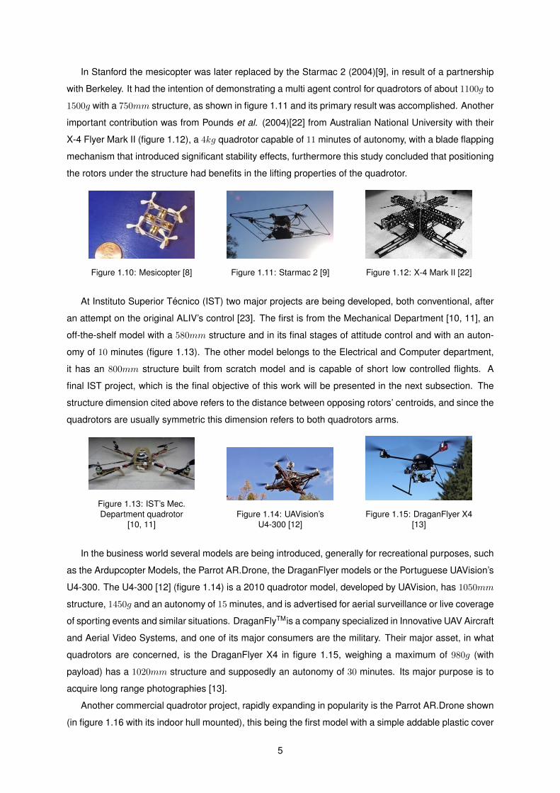
In Stanford the mesicopter was later replaced by the Starmac 2 (2004)[9], in result of a partnership

with Berkeley. It had the intention of demonstrating a multi agent control for quadrotors of about 1100g to

1500g with a 750mm structure, as shown in figure 1.11 and its primary result was accomplished. Another

important contribution was from Pounds et al. (2004)[22] from Australian National University with their

X-4 Flyer Mark II (figure 1.12), a 4kg quadrotor capable of 11 minutes of autonomy, with a blade flapping

mechanism that introduced significant stability effects, furthermore this study concluded that positioning

the rotors under the structure had benefits in the lifting properties of the quadrotor.

Figure 1.10: Mesicopter [8] Figure 1.11: Starmac 2 [9] Figure 1.12: X-4 Mark II [22]

At Instituto Superior Tecnico (IST) two major projects are being developed, both conventional, after

an attempt on the original ALIV’s control [23]. The first is from the Mechanical Department [10, 11], an

off-the-shelf model with a 580mm structure and in its final stages of attitude control and with an auton-

omy of 10 minutes (figure 1.13). The other model belongs to the Electrical and Computer department,

it has an 800mm structure built from scratch model and is capable of short low controlled flights. A

final IST project, which is the final objective of this work will be presented in the next subsection. The

structure dimension cited above refers to the distance between opposing rotors’ centroids, and since the

quadrotors are usually symmetric this dimension refers to both quadrotors arms.

Figure 1.13: IST’s Mec.Department quadrotor

[10, 11]Figure 1.14: UAVision’s

U4-300 [12]Figure 1.15: DraganFlyer X4

[13]

In the business world several models are being introduced, generally for recreational purposes, such

as the Ardupcopter Models, the Parrot AR.Drone, the DraganFlyer models or the Portuguese UAVision’s

U4-300. The U4-300 [12] (figure 1.14) is a 2010 quadrotor model, developed by UAVision, has 1050mm

structure, 1450g and an autonomy of 15 minutes, and is advertised for aerial surveillance or live coverage

of sporting events and similar situations. DraganFlyTMis a company specialized in Innovative UAV Aircraft

and Aerial Video Systems, and one of its major consumers are the military. Their major asset, in what

quadrotors are concerned, is the DraganFlyer X4 in figure 1.15, weighing a maximum of 980g (with

payload) has a 1020mm structure and supposedly an autonomy of 30 minutes. Its major purpose is to

acquire long range photographies [13].

Another commercial quadrotor project, rapidly expanding in popularity is the Parrot AR.Drone shown

(in figure 1.16 with its indoor hull mounted), this being the first model with a simple addable plastic cover

5

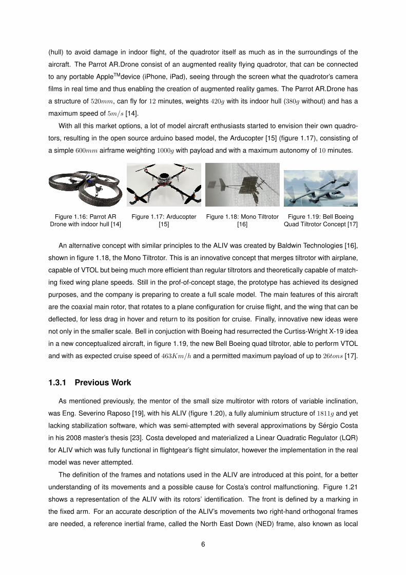
(hull) to avoid damage in indoor flight, of the quadrotor itself as much as in the surroundings of the

aircraft. The Parrot AR.Drone consist of an augmented reality flying quadrotor, that can be connected

to any portable AppleTMdevice (iPhone, iPad), seeing through the screen what the quadrotor’s camera

films in real time and thus enabling the creation of augmented reality games. The Parrot AR.Drone has

a structure of 520mm, can fly for 12 minutes, weights 420g with its indoor hull (380g without) and has a

maximum speed of 5m/s [14].

With all this market options, a lot of model aircraft enthusiasts started to envision their own quadro-

tors, resulting in the open source arduino based model, the Arducopter [15] (figure 1.17), consisting of

a simple 600mm airframe weighting 1000g with payload and with a maximum autonomy of 10 minutes.

Figure 1.16: Parrot ARDrone with indoor hull [14]

Figure 1.17: Arducopter[15]

Figure 1.18: Mono Tiltrotor[16]

Figure 1.19: Bell BoeingQuad Tiltrotor Concept [17]

An alternative concept with similar principles to the ALIV was created by Baldwin Technologies [16],

shown in figure 1.18, the Mono Tiltrotor. This is an innovative concept that merges tiltrotor with airplane,

capable of VTOL but being much more efficient than regular tiltrotors and theoretically capable of match-

ing fixed wing plane speeds. Still in the prof-of-concept stage, the prototype has achieved its designed

purposes, and the company is preparing to create a full scale model. The main features of this aircraft

are the coaxial main rotor, that rotates to a plane configuration for cruise flight, and the wing that can be

deflected, for less drag in hover and return to its position for cruise. Finally, innovative new ideas were

not only in the smaller scale. Bell in conjuction with Boeing had resurrected the Curtiss-Wright X-19 idea

in a new conceptualized aircraft, in figure 1.19, the new Bell Boeing quad tiltrotor, able to perform VTOL

and with as expected cruise speed of 463Km/h and a permitted maximum payload of up to 26tons [17].

1.3.1 Previous Work

As mentioned previously, the mentor of the small size multirotor with rotors of variable inclination,

was Eng. Severino Raposo [19], with his ALIV (figure 1.20), a fully aluminium structure of 1811g and yet

lacking stabilization software, which was semi-attempted with several approximations by Sergio Costa

in his 2008 master’s thesis [23]. Costa developed and materialized a Linear Quadratic Regulator (LQR)

for ALIV which was fully functional in flightgear’s flight simulator, however the implementation in the real

model was never attempted.

The definition of the frames and notations used in the ALIV are introduced at this point, for a better

understanding of its movements and a possible cause for Costa’s control malfunctioning. Figure 1.21

shows a representation of the ALIV with its rotors’ identification. The front is defined by a marking in

the fixed arm. For an accurate description of the ALIV’s movements two right-hand orthogonal frames

are needed, a reference inertial frame, called the North East Down (NED) frame, also known as local

6

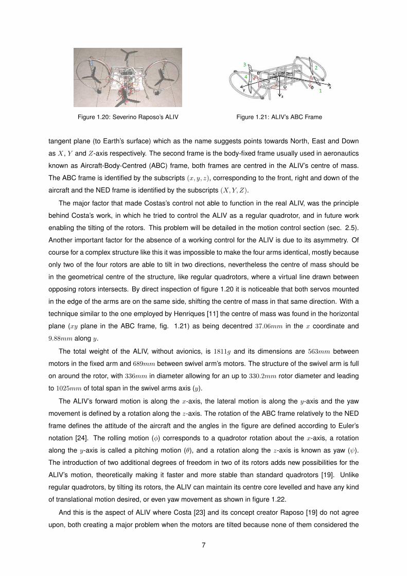
Figure 1.20: Severino Raposo’s ALIV Figure 1.21: ALIV’s ABC Frame

tangent plane (to Earth’s surface) which as the name suggests points towards North, East and Down

as X, Y and Z-axis respectively. The second frame is the body-fixed frame usually used in aeronautics

known as Aircraft-Body-Centred (ABC) frame, both frames are centred in the ALIV’s centre of mass.

The ABC frame is identified by the subscripts (x, y, z), corresponding to the front, right and down of the

aircraft and the NED frame is identified by the subscripts (X,Y, Z).

The major factor that made Costas’s control not able to function in the real ALIV, was the principle

behind Costa’s work, in which he tried to control the ALIV as a regular quadrotor, and in future work

enabling the tilting of the rotors. This problem will be detailed in the motion control section (sec. 2.5).

Another important factor for the absence of a working control for the ALIV is due to its asymmetry. Of

course for a complex structure like this it was impossible to make the four arms identical, mostly because

only two of the four rotors are able to tilt in two directions, nevertheless the centre of mass should be

in the geometrical centre of the structure, like regular quadrotors, where a virtual line drawn between

opposing rotors intersects. By direct inspection of figure 1.20 it is noticeable that both servos mounted

in the edge of the arms are on the same side, shifting the centre of mass in that same direction. With a

technique similar to the one employed by Henriques [11] the centre of mass was found in the horizontal

plane (xy plane in the ABC frame, fig. 1.21) as being decentred 37.06mm in the x coordinate and

9.88mm along y.

The total weight of the ALIV, without avionics, is 1811g and its dimensions are 563mm between

motors in the fixed arm and 689mm between swivel arm’s motors. The structure of the swivel arm is full

on around the rotor, with 336mm in diameter allowing for an up to 330.2mm rotor diameter and leading

to 1025mm of total span in the swivel arms axis (y).

The ALIV’s forward motion is along the x-axis, the lateral motion is along the y-axis and the yaw

movement is defined by a rotation along the z-axis. The rotation of the ABC frame relatively to the NED

frame defines the attitude of the aircraft and the angles in the figure are defined according to Euler’s

notation [24]. The rolling motion (φ) corresponds to a quadrotor rotation about the x-axis, a rotation

along the y-axis is called a pitching motion (θ), and a rotation along the z-axis is known as yaw (ψ).

The introduction of two additional degrees of freedom in two of its rotors adds new possibilities for the

ALIV’s motion, theoretically making it faster and more stable than standard quadrotors [19]. Unlike

regular quadrotors, by tilting its rotors, the ALIV can maintain its centre core levelled and have any kind

of translational motion desired, or even yaw movement as shown in figure 1.22.

And this is the aspect of ALIV where Costa [23] and its concept creator Raposo [19] do not agree

upon, both creating a major problem when the motors are tilted because none of them considered the

7

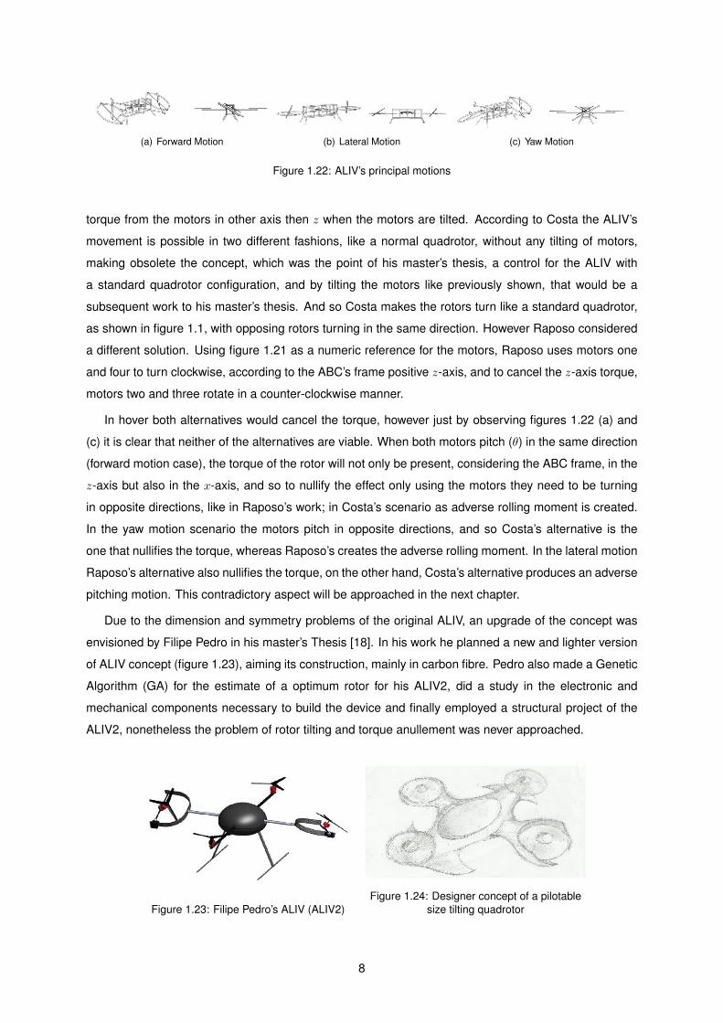
(a) Forward Motion (b) Lateral Motion (c) Yaw Motion

Figure 1.22: ALIV’s principal motions

torque from the motors in other axis then z when the motors are tilted. According to Costa the ALIV’s

movement is possible in two different fashions, like a normal quadrotor, without any tilting of motors,

making obsolete the concept, which was the point of his master’s thesis, a control for the ALIV with

a standard quadrotor configuration, and by tilting the motors like previously shown, that would be a

subsequent work to his master’s thesis. And so Costa makes the rotors turn like a standard quadrotor,

as shown in figure 1.1, with opposing rotors turning in the same direction. However Raposo considered

a different solution. Using figure 1.21 as a numeric reference for the motors, Raposo uses motors one

and four to turn clockwise, according to the ABC’s frame positive z-axis, and to cancel the z-axis torque,

motors two and three rotate in a counter-clockwise manner.

In hover both alternatives would cancel the torque, however just by observing figures 1.22 (a) and

(c) it is clear that neither of the alternatives are viable. When both motors pitch (θ) in the same direction

(forward motion case), the torque of the rotor will not only be present, considering the ABC frame, in the

z-axis but also in the x-axis, and so to nullify the effect only using the motors they need to be turning

in opposite directions, like in Raposo’s work; in Costa’s scenario as adverse rolling moment is created.

In the yaw motion scenario the motors pitch in opposite directions, and so Costa’s alternative is the

one that nullifies the torque, whereas Raposo’s creates the adverse rolling moment. In the lateral motion

Raposo’s alternative also nullifies the torque, on the other hand, Costa’s alternative produces an adverse

pitching motion. This contradictory aspect will be approached in the next chapter.

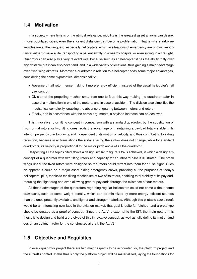
Due to the dimension and symmetry problems of the original ALIV, an upgrade of the concept was

envisioned by Filipe Pedro in his master’s Thesis [18]. In his work he planned a new and lighter version

of ALIV concept (figure 1.23), aiming its construction, mainly in carbon fibre. Pedro also made a Genetic

Algorithm (GA) for the estimate of a optimum rotor for his ALIV2, did a study in the electronic and

mechanical components necessary to build the device and finally employed a structural project of the

ALIV2, nonetheless the problem of rotor tilting and torque anullement was never approached.

Figure 1.23: Filipe Pedro’s ALIV (ALIV2)Figure 1.24: Designer concept of a pilotable

size tilting quadrotor

8

1.4 Motivation

In a society where time is of the utmost relevance, mobility is the greatest asset anyone can desire.

In overpopulated cities, even the shortest distances can become problematic. That is where airborne

vehicles are at the vanguard, especially helicopters, which in situations of emergency are of most impor-

tance, either to save a life transporting a patient swiftly to a nearby hospital or even aiding in a fire-fight.

Quadrotors can also play a very relevant role, because such as an helicopter, it has the ability to fly over

any obstacle but it can also hover and land in a wide variety of locations, thus gaining a major advantage

over fixed wing aircrafts. Moreover a quadrotor in relation to a helicopter adds some major advantages,

considering the same hypothetical dimensionality:

• Absence of tail rotor, hence making it more energy efficient, instead of the usual helicopter’s tail

yaw control;

• Division of the propelling mechanisms, from one to four, this way making the quadrotor safer in

case of a malfunction in one of the motors, and in case of accident. The division also simplifies the

mechanical complexity, enabling the absence of gearing between motors and rotors;

• Finally, and in accordance with the above arguments, a payload increase can be achieved.

This innovative rotor tilting concept in comparison with a standard quadrotor, by the substitution of

two normal rotors for two tilting ones, adds the advantage of maintaining a payload totally stable in its

interior, perpendicular to gravity, and independent of its motion or velocity, and thus contributing to a drag

reduction, because in all translations the surface facing the airflow does not change, while for standard

quadrotors, its velocity is proportional to the roll or pitch angle of all the quadrotor.

Respecting all the topics cited above a design similar to figure 1.24 is achieved, in which a designer’s

concept of a quadrotor with two tilting rotors and capacity for an inboard pilot is illustrated. The small

wings under the fixed rotors were designed so the rotors could retract into them for cruise flight. Such

an apparatus could be a major asset aiding emergency crews, providing all the purposes of today’s

helicopters, plus, thanks to the tilting mechanism of two of its rotors, enabling total stability of its payload,

reducing the flight drag and even allowing greater payloads through the existence of four motors.

All these advantages of the quadrotors regarding regular helicopters could not come without some

drawbacks, such as some weight penalty, which can be minimized by more energy efficient sources

than the ones presently available, and lighter and stronger materials. Although this pilotable size aircraft

would be an interesting new face in the aviation market, that goal is quite far-fetched, and a prototype

should be created as a proof-of-concept. Since the ALIV is external to the IST, the main goal of this

thesis is to design and build a prototype of this innovative concept, as well as fully define its motion and

design an optimum rotor for the constructed aircraft, the ALIV3.

1.5 Objective and Requisites

In every quadrotor project there are two major aspects to be accounted for, the platform project and

the aircraft’s control. In this thesis only the platform project will be materialized, laying the foundations for

9

the implementation of a control via a correct and applicable conceptualized motion, through rotor tilting,

and never forgetting the rotor’s torque.

As said previously, the goal of this thesis is to improve Pedro’s concept when possible, and build

a quadrotor with tilting movements in two directions in a pair of opposing rotors. A structural analysis

should be conducted and the design of an optimum rotor should be achieved. Finally a full determination

of the possible movements of the aircraft shall be completed. The quadrotor itself, the ALIV3, should be

built with the following considerations, in accordance with Pedro’s [18] and Raposo’s [19] works:

Maximum weight (without payload) 1800g

Minimum endurance 10 minutes

Maximum translational and climb speed needed 10m.s−1 and 5m.s−1

Payload Camera (Video, Infra-red, Night vision)

Table 1.1: ALIV3 project requisits

1.6 Thesis Structure

In this chapter the key concepts used for this project, namely the quadrotor and tiltrotor are intro-

duced. An historical overview and a state-of-the-art review of these concepts are conducted and the

previous versions of the ALIV3’s concept, to be fully designed and constructed, are described. Lastly

this chapter enlightens the motivation, objectives and requisites for the ALIV3.

Chapter 2 is focused on the preliminary design of the ALIV3, its components maximum dimensions as

well as their initially envisioned shapes are explained. A few swivel arm alternatives are introduced and

a full motion determination is conducted with all possible movements of the ALIV3 are fully explained.

Chapter 3 is dedicated to the creation of an optimum rotor for the ALIV3. The choice of its aerofoil and

all the remaining crucial geometric or operational variables are acquired, using the blade element mo-

mentum theory and a genetic algorithm solver, with the intention of building the virtual three-dimensional

model in a rapid prototyping process.

All ALIV3 components that do not demand a precise design, or are very hard, or almost impossible to

create, such as electronics, motors, and servos are selected in chapter 4, with a thorough and concise

selection process for every component.

In chapter 5 all original designed components, and respective casts are depicted, and some dimen-

sional decisions are sustained by a finite element method analysis.

The ALIV3 constructed models are evaluated and a performance analysis to the forward flight and

climbing motion are executed in chapter 6. The servo’s maximum torque and the drag of both alternatives

is also studied to determine which arm alternative is the most suited to accomplish the design goals more

efficiently. Also the drag analysis will study the gains of adding a cover to the ALIV3’s central area.

The conclusions and a future work section close this thesis in chapter 7.

10

Chapter 2

Preliminary Design

The creation of the ALIV3 structure started with a revision of Filipe Pedro’s [18] concept (figure 1.23),

as well as of all the other relevant models previously depicted, with the aim of redesigning and building

a working quadrotor. The structural concepts were divided in three major areas: the central area, where

all the avionic components are located and where the arms and the landing gear converge; the swivel

arm, the most important issue of this project, and what makes the ALIV3 unique; and finally the landing

gear, to prevent any damage to the other ALIV3’s components.

2.1 Principal Structural Dimensions

The first step was the definition of the prototype’s dimensions. The original ALIV had 563mm between

rotors in the fixed arm and 689mm between swivel arm’s rotors, making it very unstable dynamically [19]

while Pedro’s ALIV2 had an 800mm by 800mm structure. There is no specific method for choosing these

dimensions, nonetheless in standard quadrotors their greatest impact is in the pitching or rolling angular

speeds, the longer the arm, the larger the moment and so the greater the angular speed. On the other

hand with a larger arm, the greater the tensions in the structure, thus obliging for a more robust structure

and therefore more structural weight. In ALIV3’s case angular speed for rolling or pitching movements is

not of great importance, because the translational motion is achieved by the motor-rotor couple tilt and

not by aircraft tilting, and so the 800mm structure seems to be too large for what the ALIV3 requires or

an optimal structure needs.

Referring to the most recent quadrotors [23, 10, 11, 15], all have a smaller, symmetrical structure.

The Arducopter, the open source quadrotor has 600mm, the Parrot AR.Drone has 520mm and IST’s

Mechanical Department quadrotor has 580mm. In accordance with this dimensions, it was decided that

the ALIV3 structure would have 600mm, firstly to make it compatible with the Arducopter software, and

secondly,in the absence of a theoretically strong principle behind this option, analysing the evolution of

recent quadrotor models, all exhibit smaller dimensions, around the 520mm to 600mm range, whereas

previous models had roughly 1000mm. The ALIV3’s total height will depend on the space needed for

electronic components and landing gear design, while the final weight will depend on the arms and

11

landing gear design, and also the weight of all the indispensable components.

2.2 Swivel Arm Concept

The most important aspects of the ALIV3, mainly what makes the ALIV3 unique, are its swivel arms,

capable of tilting the rotor in two directions.

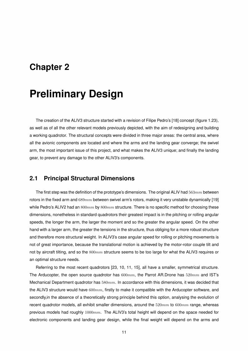
In the original Raposo’s concept (figure 2.1) the motor was placed inside a full circle aluminium frame,

with the motor connected to a tube in turn connected to the frame in two positions, 180o apart. These

connections allowed the rotation of the motor in the tube axis, referred in section 1.3.1 as the responsible

for the lateral motion. This rotation is allowed by a servo, known as the second-servo, which is mounted

in the circular aluminium.

Perpendicular to this tube, 90o from the its connections with the circular aluminium frame, a tube runs

from the outer side of the circle, towards the central area of the ALIV, this tube is also connected to a

servo (defined as the first-servo) and tilts the motor-rotor couple, and all the rest of the arm, allowing the

previous described forward motion. Pedro realised that a full circle, while protecting the rotor in case of

accident was an excess of weight that could be averted, and so in his design the full circle is replaced

by a half circle (figure 2.2).

Figure 2.1: Raposo’s ALIV swivel arm Figure 2.2: Pedro’s ALIV2 swivel arm

Some alternatives to Pedro’s design were envisioned and will be depicted in the next subsections.

Firstly it is necessary to determine the maximum rotor size and also the maximum tilt of the rotor (and

motor) as dimension limitations for the arm. According to Aeroquad [25] (from the Arducopter family), for

a general use, the standard rotor has 10 inches (254mm), while for heavy payloads a 12 inch (304.8mm)

rotor is more appropriate, nonetheless in the ALIV2 the arm had just 220mm and in the ALIV 336mm.

So to accommodate the best option (254mm) and still have a margin for the servo, the maximum rotor

size which will determine the size of an arm similar to the one from ALIV2 will be 11in (279.4mm).

The maximum tilting angle of the rotor has two consequences, firstly it will influence the servo needed

for such a rotation and secondly it could prevent different designs where a 360o rotation cannot be

achieved, but the goal of tilting rotors is accomplished. In Pedro’s work is referred that the maximum

tilting angle with the vertical in any direction is 62o, and so this will be the angle to take into consideration

in the next subsection where alternatives to the ALIV2 swivel arm, also known as U-arm, will be depicted.

12

2.2.1 The U-arm

Figure 2.2 represents the U-arm, that as the the name states is a U shaped form, connected by

its middle to a servo, the first-servo, which is attached to the main structure, and through that servo’s

rotation pitches (θ) the arm to achieve the forward flight motion. The lateral motion is acquired by another

servo action, placed in the tip of the U, the second-servo, that is connected to the other U’s end with

a tube, while free to rotate. This rotation will roll (φ) the motor-rotor couple, that must stand on this

connection. Two different alternatives for its placement were envisioned.

The first alternative is a simple connection with a carbon plate embracing the tube (glued or screwed

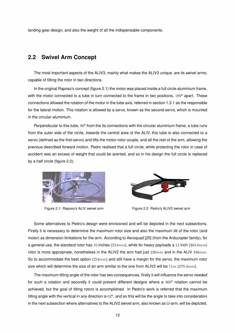
to it) (figure 2.3(a)) which is the simplest way to connect efficiently the motor to the rest of the arm without

many technical or construction abnormalities. This simplistic junction has exactly that in its favour, its

simplicity, nonetheless the major torque producer, the rotor, is placed far from both servo’s tilting axis,

what would increase the torque that the servo needed to do, to tilt the motor and rotor.

(a) Embracing plate (b) Motor in box

Figure 2.3: Possible motor connections for the U-arm

To avoid this situation an alternative was envisioned, that could place the rotor’s center of rotation

closer to the tube. This solution places the motor inside a box, cut the tube where a hypothetical line

from the first-servo would intersect it and place the box in its place, see figure 2.3(b). This alternative

would decrease the moment effect from the rotor’s rotation because the rotor itself would be closer to

the rotating axis from both servos. On the other hand the structural complexity is increased as well as

the construction problems. Instead of one tube with a motor in the middle, now two smaller tubes and a

box need to be perfectly balanced and rotated by servo action.

Both alternatives will be exploited in the design and construction phase, in chapter 5. In the ALIV2

project this connection was made with the motor clamped to a very slim rod and such a connection

would be very difficult to produce with the technology available in the Aerospace Laboratory.

The other aspect of importance in the U shaped design is the U itself. Its dimensions are mainly

determined by the maximum rotor size previously set as 279.4mm. Since the servo needs to be attached

to the arm’s end, that same section cannot be curved, as well as the the U’s opposite tip for symmetry

reasons. So as is shown in figure 2.2, both ends of the U are straight and the maximum distance between

the arm tips should never surpass 279.4mm, and the tip’s straight section must be slightly larger than

the selected servo’s height. The middle of the U needs to be straight as well to allow a connection to

the main structure, and its dimension equals the tip straight section so that the U curvature remains a

quarter circle.

The distance between the middle of the U and the connection of the second-servo is supposed to be

13

half the size of the rotor, about 139.7mm. The thickness of this structure (as well as all possible designs

envisioned from henceforth) will be designed with a Finite Element Method (FEM) analysis in chapter 5.

The width of the model is decided based on the servo’s width. The maximum tilting angle of the motor

and rotor in this design is not important because both servos’ movement are not constrained by any

structural component and so the rotor is free to tilt 360o from both servos’ action.

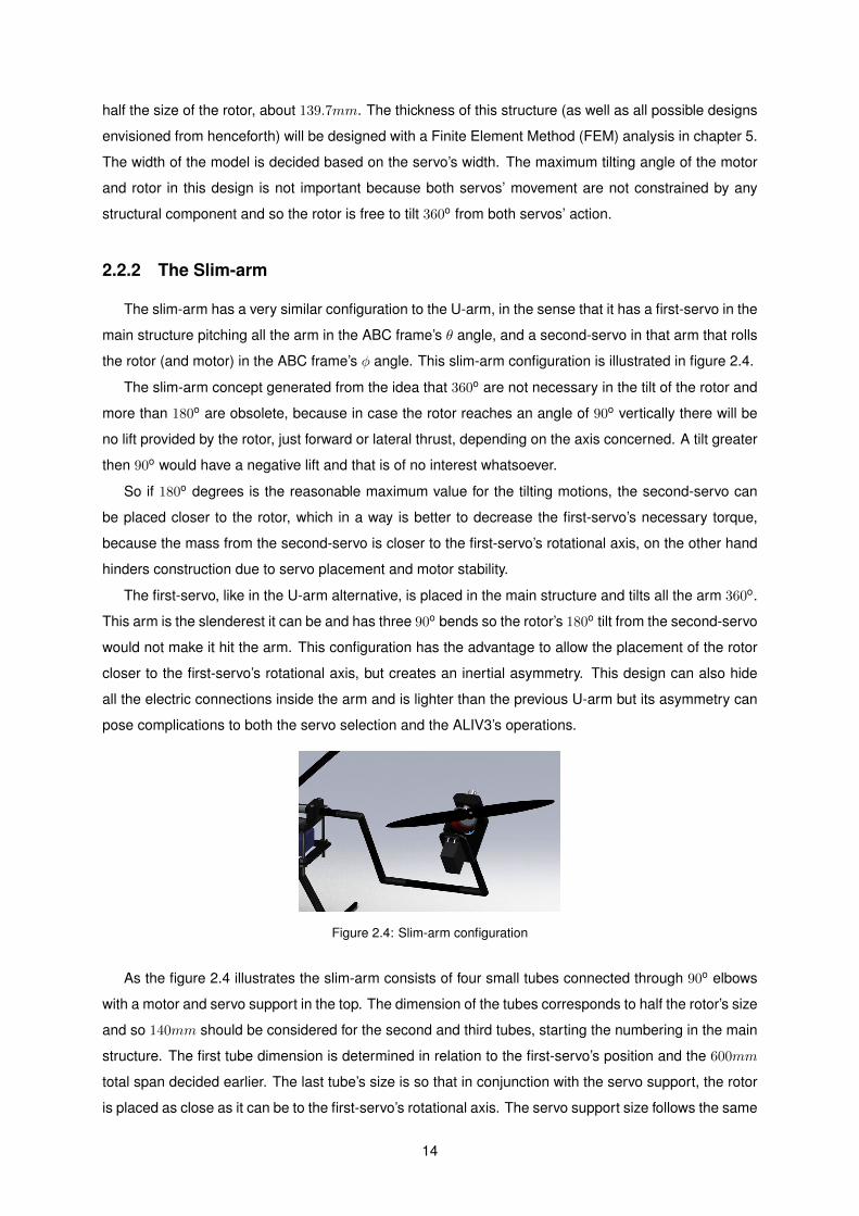
2.2.2 The Slim-arm

The slim-arm has a very similar configuration to the U-arm, in the sense that it has a first-servo in the

main structure pitching all the arm in the ABC frame’s θ angle, and a second-servo in that arm that rolls

the rotor (and motor) in the ABC frame’s φ angle. This slim-arm configuration is illustrated in figure 2.4.

The slim-arm concept generated from the idea that 360o are not necessary in the tilt of the rotor and

more than 180o are obsolete, because in case the rotor reaches an angle of 90o vertically there will be

no lift provided by the rotor, just forward or lateral thrust, depending on the axis concerned. A tilt greater

then 90o would have a negative lift and that is of no interest whatsoever.

So if 180o degrees is the reasonable maximum value for the tilting motions, the second-servo can

be placed closer to the rotor, which in a way is better to decrease the first-servo’s necessary torque,

because the mass from the second-servo is closer to the first-servo’s rotational axis, on the other hand

hinders construction due to servo placement and motor stability.

The first-servo, like in the U-arm alternative, is placed in the main structure and tilts all the arm 360o.

This arm is the slenderest it can be and has three 90o bends so the rotor’s 180o tilt from the second-servo

would not make it hit the arm. This configuration has the advantage to allow the placement of the rotor

closer to the first-servo’s rotational axis, but creates an inertial asymmetry. This design can also hide

all the electric connections inside the arm and is lighter than the previous U-arm but its asymmetry can

pose complications to both the servo selection and the ALIV3’s operations.

Figure 2.4: Slim-arm configuration

As the figure 2.4 illustrates the slim-arm consists of four small tubes connected through 90o elbows

with a motor and servo support in the top. The dimension of the tubes corresponds to half the rotor’s size

and so 140mm should be considered for the second and third tubes, starting the numbering in the main

structure. The first tube dimension is determined in relation to the first-servo’s position and the 600mm

total span decided earlier. The last tube’s size is so that in conjunction with the servo support, the rotor

is placed as close as it can be to the first-servo’s rotational axis. The servo support size follows the same

14

rule as the straight portion of the U-arm. It needs to be as large as the servo selected needs it to be, and

the motor is placed in a similar fashion to the U-arm, with a simple embracing plate or with the motor in

box configuration. This second arm approach has the advantage of the motor positioning regarding the

first-servo’s rotational, however regarding the second-servo the situation is exactly the same as in the

U-arm.

This slim-arm alternative can rotate the rotor 360o in the θ angle and 180o in the φ angle, is lighter

than the U-arm but has an asymmetry that can jeopardise the servo selection, nonetheless is a valid

and executable solution.

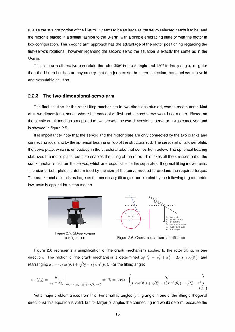
2.2.3 The two-dimensional-servo-arm

The final solution for the rotor tilting mechanism in two directions studied, was to create some kind

of a two-dimensional servo, where the concept of first and second-servo would not matter. Based on

the simple crank mechanism applied to two servos, the two-dimensional-servo-arm was conceived and

is showed in figure 2.5.

It is important to note that the servos and the motor plate are only connected by the two cranks and

connecting rods, and by the spherical bearing on top of the structural rod. The servos sit on a lower plate,

the servo plate, which is embedded in the structural tube that comes from below. The spherical bearing

stabilizes the motor place, but also enables the tilting of the rotor. This takes all the stresses out of the

crank mechanisms from the servos, which are responsible for the separate orthogonal tilting movements.

The size of both plates is determined by the size of the servo needed to produce the required torque.

The crank mechanism is as large as the necessary tilt angle, and is ruled by the following trigonometric

law, usually applied for piston motion.

Figure 2.5: 2D-servo-armconfiguration

R

rod lenghtpiston positioncrank radiusmotor plate radiusmotor plate anglecrank angle

c

c

cc

cc

c

c

c

c

c

c

c

Figure 2.6: Crank mechanism simplification

Figure 2.6 represents a simplification of the crank mechanism applied to the rotor tilting, in one

direction. The motion of the crank mechanism is determined by l2c = r2c + x2

c − 2rcxc cos(θc), and

rearranging xc = rc cos(θc) +√l2c − r2

c sin2(θc). For the tilting angle:

tan(βc) =Rc

xc − x0c

∣∣∣∣x0c=xc(θc=90)=

√l2c−r2

c

⇒ βc = arctan

(Rc

rccos(θc) +√l2c − r2

csin2(θc)−

√l2c − r2

c

)(2.1)

Yet a major problem arises from this. For small βc angles (tilting angle in one of the tilting orthogonal

directions) this equation is valid, but for larger βc angles the connecting rod would deform, because the

15

motor plate would maintain its dimension. This can be averted by letting the link of the connecting rod

with the motor plate slide along the plate, maintaining the crank and connecting rod in the same plane,

without deformation.

Another problem is the spherical bearing. While it increases the structural integrity of the concept, it

also decreases its tilting ability. This is explained because its rotation is limited by its size in comparison

with the tube that it is connected to, and the bigger the bearing the heavier the structure.

The connection to the main structure is done by a elbow junction at the end of the connecting tube,

that has a dimension determined by the maximum tilting angle possible and the motor plate size. The

advantage of this design is that the connection to the main structure is static, embedded in all degrees

of freedom and so structurally simpler that the servo connections of the previous alternatives.

The two-dimensional-servo-arm configuration is an innovative concept, but very hard to build, its

servos can rotate the motor through a crank mechanism that enables them to a tilting motion in both

directions however inferior to 180o.

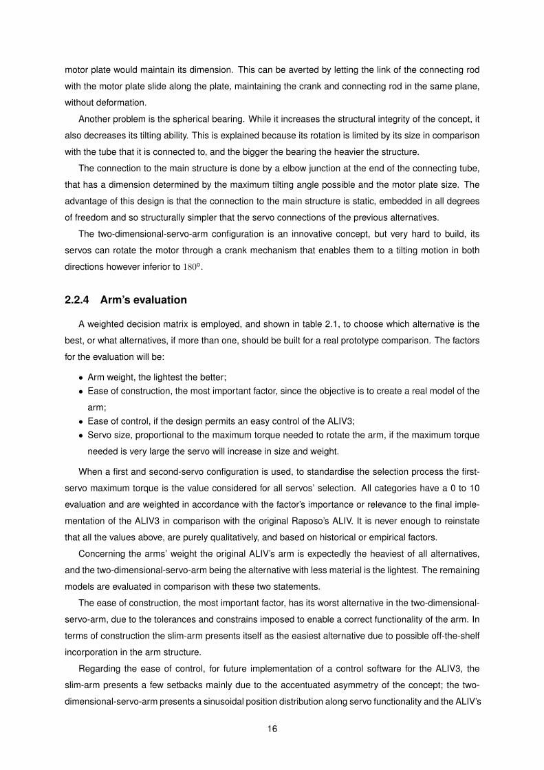
2.2.4 Arm’s evaluation

A weighted decision matrix is employed, and shown in table 2.1, to choose which alternative is the

best, or what alternatives, if more than one, should be built for a real prototype comparison. The factors

for the evaluation will be:

• Arm weight, the lightest the better;• Ease of construction, the most important factor, since the objective is to create a real model of the

arm;• Ease of control, if the design permits an easy control of the ALIV3;• Servo size, proportional to the maximum torque needed to rotate the arm, if the maximum torque

needed is very large the servo will increase in size and weight.

When a first and second-servo configuration is used, to standardise the selection process the first-

servo maximum torque is the value considered for all servos’ selection. All categories have a 0 to 10

evaluation and are weighted in accordance with the factor’s importance or relevance to the final imple-

mentation of the ALIV3 in comparison with the original Raposo’s ALIV. It is never enough to reinstate

that all the values above, are purely qualitatively, and based on historical or empirical factors.

Concerning the arms’ weight the original ALIV’s arm is expectedly the heaviest of all alternatives,

and the two-dimensional-servo-arm being the alternative with less material is the lightest. The remaining

models are evaluated in comparison with these two statements.

The ease of construction, the most important factor, has its worst alternative in the two-dimensional-

servo-arm, due to the tolerances and constrains imposed to enable a correct functionality of the arm. In

terms of construction the slim-arm presents itself as the easiest alternative due to possible off-the-shelf

incorporation in the arm structure.

Regarding the ease of control, for future implementation of a control software for the ALIV3, the

slim-arm presents a few setbacks mainly due to the accentuated asymmetry of the concept; the two-

dimensional-servo-arm presents a sinusoidal position distribution along servo functionality and the ALIV’s

16

Arm alternative

Atributes (Relative Weighting)

TotalWeight Ease of Ease of Control Servo Size

(25%) Construction (45%) (30%) (10%)

ALIV’s arm 5 5 5 5 5

U-arm 6 7 7 6 6.65

Slim-arm 8 8 3 3 6.5

2D-arm 10 1 3 10 4.85

Table 2.1: Arm’s weighted decision matrix

arm, its simplification, the U-arm presents a clear improvement due to the underlying weight loss. Finally

in terms of servo size, the two-dimensional-servo-arm is obviously the best option, since both servos

are located near the motor. Its maximum torque requisites, will be much lower than all the other options.

The slim-arm first-servo will have the worst result, due to the asymmetry of the arm itself.

As expected the two-dimensional-servo-arm is the most penalized design, mainly because the con-

struction of such model would exceed the conditions of the laboratory where the work would be done,

and thereby its fully realization in working conditions would be very hard to achieve, so its further de-

sign and construction shall not be pursued. The other two designs, the U-arm and the slim-arm, will be

further studied in chapter 5 with the ultimate goal of construction.

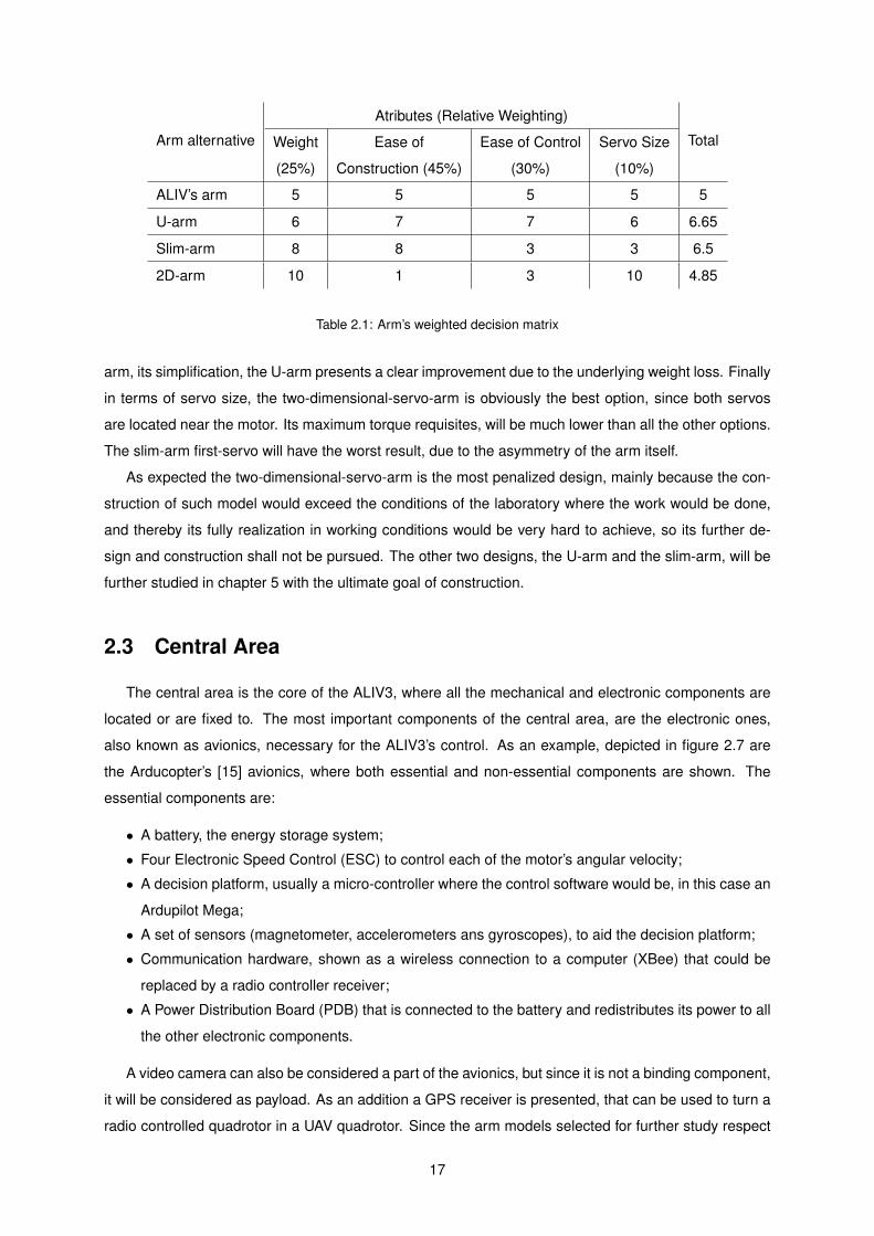
2.3 Central Area

The central area is the core of the ALIV3, where all the mechanical and electronic components are

located or are fixed to. The most important components of the central area, are the electronic ones,

also known as avionics, necessary for the ALIV3’s control. As an example, depicted in figure 2.7 are

the Arducopter’s [15] avionics, where both essential and non-essential components are shown. The

essential components are:

• A battery, the energy storage system;

• Four Electronic Speed Control (ESC) to control each of the motor’s angular velocity;

• A decision platform, usually a micro-controller where the control software would be, in this case an

Ardupilot Mega;

• A set of sensors (magnetometer, accelerometers ans gyroscopes), to aid the decision platform;

• Communication hardware, shown as a wireless connection to a computer (XBee) that could be

replaced by a radio controller receiver;

• A Power Distribution Board (PDB) that is connected to the battery and redistributes its power to all

the other electronic components.

A video camera can also be considered a part of the avionics, but since it is not a binding component,

it will be considered as payload. As an addition a GPS receiver is presented, that can be used to turn a

radio controlled quadrotor in a UAV quadrotor. Since the arm models selected for further study respect

17

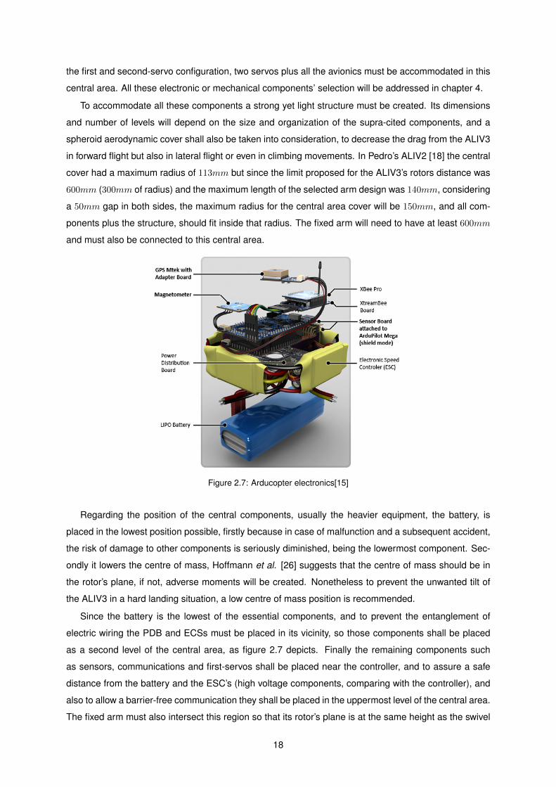
the first and second-servo configuration, two servos plus all the avionics must be accommodated in this

central area. All these electronic or mechanical components’ selection will be addressed in chapter 4.

To accommodate all these components a strong yet light structure must be created. Its dimensions

and number of levels will depend on the size and organization of the supra-cited components, and a

spheroid aerodynamic cover shall also be taken into consideration, to decrease the drag from the ALIV3

in forward flight but also in lateral flight or even in climbing movements. In Pedro’s ALIV2 [18] the central

cover had a maximum radius of 113mm but since the limit proposed for the ALIV3’s rotors distance was

600mm (300mm of radius) and the maximum length of the selected arm design was 140mm, considering

a 50mm gap in both sides, the maximum radius for the central area cover will be 150mm, and all com-

ponents plus the structure, should fit inside that radius. The fixed arm will need to have at least 600mm

and must also be connected to this central area.

Figure 2.7: Arducopter electronics[15]

Regarding the position of the central components, usually the heavier equipment, the battery, is

placed in the lowest position possible, firstly because in case of malfunction and a subsequent accident,

the risk of damage to other components is seriously diminished, being the lowermost component. Sec-

ondly it lowers the centre of mass, Hoffmann et al. [26] suggests that the centre of mass should be in

the rotor’s plane, if not, adverse moments will be created. Nonetheless to prevent the unwanted tilt of

the ALIV3 in a hard landing situation, a low centre of mass position is recommended.

Since the battery is the lowest of the essential components, and to prevent the entanglement of

electric wiring the PDB and ECSs must be placed in its vicinity, so those components shall be placed

as a second level of the central area, as figure 2.7 depicts. Finally the remaining components such

as sensors, communications and first-servos shall be placed near the controller, and to assure a safe

distance from the battery and the ESC’s (high voltage components, comparing with the controller), and

also to allow a barrier-free communication they shall be placed in the uppermost level of the central area.

The fixed arm must also intersect this region so that its rotor’s plane is at the same height as the swivel

18

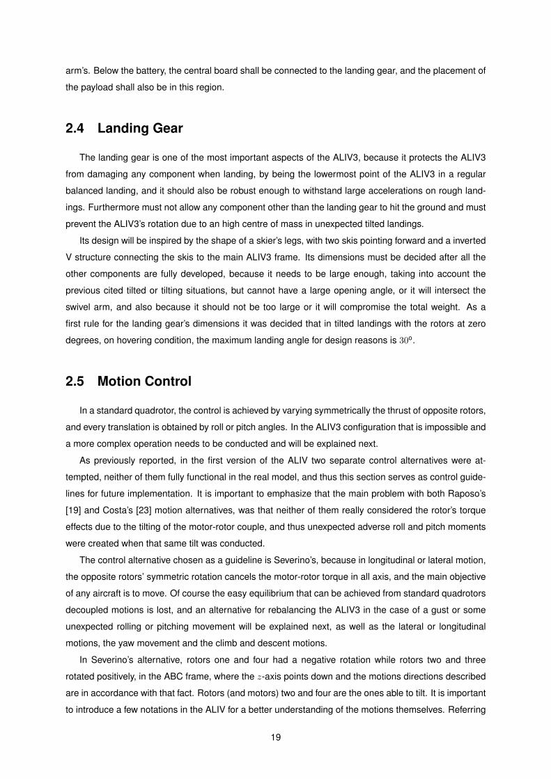
arm’s. Below the battery, the central board shall be connected to the landing gear, and the placement of

the payload shall also be in this region.

2.4 Landing Gear

The landing gear is one of the most important aspects of the ALIV3, because it protects the ALIV3

from damaging any component when landing, by being the lowermost point of the ALIV3 in a regular

balanced landing, and it should also be robust enough to withstand large accelerations on rough land-

ings. Furthermore must not allow any component other than the landing gear to hit the ground and must

prevent the ALIV3’s rotation due to an high centre of mass in unexpected tilted landings.

Its design will be inspired by the shape of a skier’s legs, with two skis pointing forward and a inverted

V structure connecting the skis to the main ALIV3 frame. Its dimensions must be decided after all the

other components are fully developed, because it needs to be large enough, taking into account the

previous cited tilted or tilting situations, but cannot have a large opening angle, or it will intersect the

swivel arm, and also because it should not be too large or it will compromise the total weight. As a

first rule for the landing gear’s dimensions it was decided that in tilted landings with the rotors at zero

degrees, on hovering condition, the maximum landing angle for design reasons is 30o.

2.5 Motion Control

In a standard quadrotor, the control is achieved by varying symmetrically the thrust of opposite rotors,

and every translation is obtained by roll or pitch angles. In the ALIV3 configuration that is impossible and

a more complex operation needs to be conducted and will be explained next.

As previously reported, in the first version of the ALIV two separate control alternatives were at-

tempted, neither of them fully functional in the real model, and thus this section serves as control guide-

lines for future implementation. It is important to emphasize that the main problem with both Raposo’s

[19] and Costa’s [23] motion alternatives, was that neither of them really considered the rotor’s torque

effects due to the tilting of the motor-rotor couple, and thus unexpected adverse roll and pitch moments

were created when that same tilt was conducted.

The control alternative chosen as a guideline is Severino’s, because in longitudinal or lateral motion,

the opposite rotors’ symmetric rotation cancels the motor-rotor torque in all axis, and the main objective

of any aircraft is to move. Of course the easy equilibrium that can be achieved from standard quadrotors

decoupled motions is lost, and an alternative for rebalancing the ALIV3 in the case of a gust or some

unexpected rolling or pitching movement will be explained next, as well as the lateral or longitudinal

motions, the yaw movement and the climb and descent motions.

In Severino’s alternative, rotors one and four had a negative rotation while rotors two and three

rotated positively, in the ABC frame, where the z-axis points down and the motions directions described

are in accordance with that fact. Rotors (and motors) two and four are the ones able to tilt. It is important

to introduce a few notations in the ALIV for a better understanding of the motions themselves. Referring

19

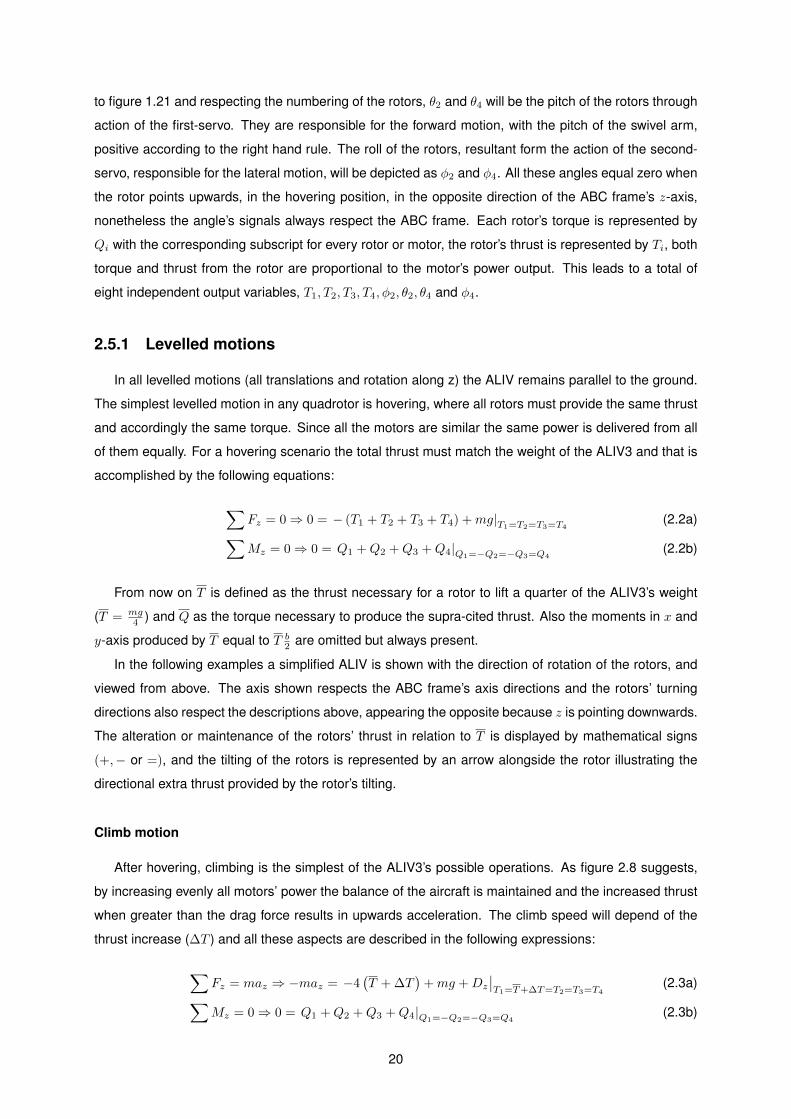
to figure 1.21 and respecting the numbering of the rotors, θ2 and θ4 will be the pitch of the rotors through

action of the first-servo. They are responsible for the forward motion, with the pitch of the swivel arm,

positive according to the right hand rule. The roll of the rotors, resultant form the action of the second-

servo, responsible for the lateral motion, will be depicted as φ2 and φ4. All these angles equal zero when

the rotor points upwards, in the hovering position, in the opposite direction of the ABC frame’s z-axis,

nonetheless the angle’s signals always respect the ABC frame. Each rotor’s torque is represented by

Qi with the corresponding subscript for every rotor or motor, the rotor’s thrust is represented by Ti, both

torque and thrust from the rotor are proportional to the motor’s power output. This leads to a total of

eight independent output variables, T1, T2, T3, T4, φ2, θ2, θ4 and φ4.

2.5.1 Levelled motions

In all levelled motions (all translations and rotation along z) the ALIV remains parallel to the ground.

The simplest levelled motion in any quadrotor is hovering, where all rotors must provide the same thrust

and accordingly the same torque. Since all the motors are similar the same power is delivered from all

of them equally. For a hovering scenario the total thrust must match the weight of the ALIV3 and that is

accomplished by the following equations:

∑Fz = 0⇒ 0 = − (T1 + T2 + T3 + T4) +mg|T1=T2=T3=T4

(2.2a)∑Mz = 0⇒ 0 = Q1 +Q2 +Q3 +Q4|Q1=−Q2=−Q3=Q4

(2.2b)

From now on T is defined as the thrust necessary for a rotor to lift a quarter of the ALIV3’s weight

(T = mg4 ) and Q as the torque necessary to produce the supra-cited thrust. Also the moments in x and

y-axis produced by T equal to T b2 are omitted but always present.

In the following examples a simplified ALIV is shown with the direction of rotation of the rotors, and

viewed from above. The axis shown respects the ABC frame’s axis directions and the rotors’ turning

directions also respect the descriptions above, appearing the opposite because z is pointing downwards.

The alteration or maintenance of the rotors’ thrust in relation to T is displayed by mathematical signs

(+,− or =), and the tilting of the rotors is represented by an arrow alongside the rotor illustrating the

directional extra thrust provided by the rotor’s tilting.

Climb motion

After hovering, climbing is the simplest of the ALIV3’s possible operations. As figure 2.8 suggests,

by increasing evenly all motors’ power the balance of the aircraft is maintained and the increased thrust

when greater than the drag force results in upwards acceleration. The climb speed will depend of the

thrust increase (∆T ) and all these aspects are described in the following expressions:

∑Fz = maz ⇒ −maz = −4

(T + ∆T

)+mg +Dz

∣∣T1=T+∆T=T2=T3=T4

(2.3a)∑Mz = 0⇒ 0 = Q1 +Q2 +Q3 +Q4|Q1=−Q2=−Q3=Q4

(2.3b)

20

Figure 2.8: ALIV3’s climb motion control

To descent it is only necessary to decrease the total thrust evenly: the higher the decrease the

faster the descent. To maintain a steady climb or descent, with constant velocity, az must be null with

4∆T = Dz to maintain the z-axis velocity.

Forward motion

In forward levelled motion, the tilting of the rotors is responsible for the motion itself, through an

increase in thrust and a pitching angle (θi) of both rotors, two and four. The increase in thrust must be

such that the lift (z-axis) component must remain as it was before tilting, for two reasons: to maintain the

ALIV3 levelled its total weight must remain equal to the lift, and secondly to maintain the torque in the

z-axis null. The x-axis torque is symmetric in both tilted rotors and thus null, and the moment created

through the forward thrust is symmetric for both rotors and thus cancelled. The distance between rotors

(or motors), from now on is represented as l, and was defined previously as 600mm. The following

equations rule the forward motion case:

∑Fx = max ⇒ max = T2 sin θ2 + T4 sin θ4 −Dx|T2 sin θ2=T4 sin θ4=∆T,θ2=θ4

(2.4a)∑Fz = 0⇒ 0 = − (T1 + T2 cos θ2 + T3 + T4 cos θ4) +mg|T1=T=T2 cos θ2=T3=T4 cos θ4

(2.4b)∑Mx = 0⇒ 0 = Q2 sin θ2 +Q4 sin θ4|Q2=−Q4

(2.4c)∑Mz = 0⇒ 0 = Q1 +Q2 cos θ2 +Q3 +Q4 cos θ4 +

b

2(T2 sin θ2 − T4 sin θ4)

∣∣∣∣Q1=Q=−Q3

(2.4d)

Figure 2.9: ALIV3’s forward motion control

21

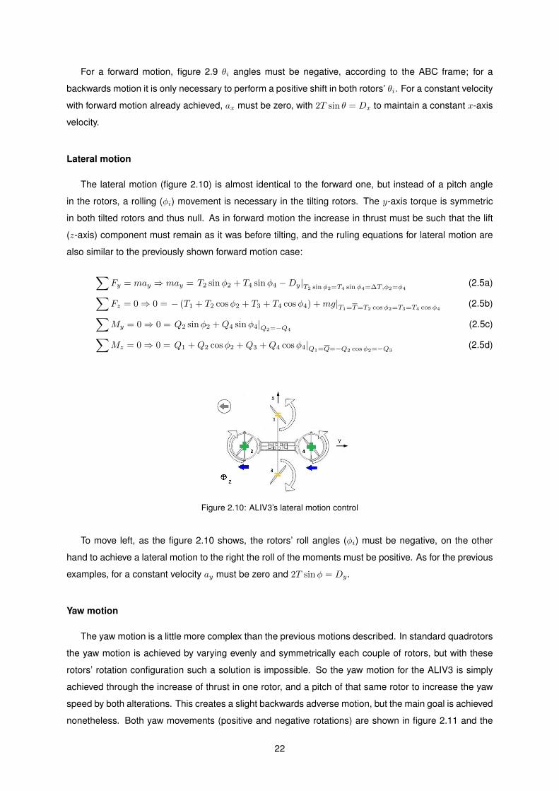
For a forward motion, figure 2.9 θi angles must be negative, according to the ABC frame; for a

backwards motion it is only necessary to perform a positive shift in both rotors’ θi. For a constant velocity

with forward motion already achieved, ax must be zero, with 2T sin θ = Dx to maintain a constant x-axis

velocity.

Lateral motion

The lateral motion (figure 2.10) is almost identical to the forward one, but instead of a pitch angle

in the rotors, a rolling (φi) movement is necessary in the tilting rotors. The y-axis torque is symmetric

in both tilted rotors and thus null. As in forward motion the increase in thrust must be such that the lift

(z-axis) component must remain as it was before tilting, and the ruling equations for lateral motion are

also similar to the previously shown forward motion case:

∑Fy = may ⇒ may = T2 sinφ2 + T4 sinφ4 −Dy|T2 sinφ2=T4 sinφ4=∆T,φ2=φ4

(2.5a)∑Fz = 0⇒ 0 = − (T1 + T2 cosφ2 + T3 + T4 cosφ4) +mg|T1=T=T2 cosφ2=T3=T4 cosφ4

(2.5b)∑My = 0⇒ 0 = Q2 sinφ2 +Q4 sinφ4|Q2=−Q4

(2.5c)∑Mz = 0⇒ 0 = Q1 +Q2 cosφ2 +Q3 +Q4 cosφ4|Q1=Q=−Q2 cosφ2=−Q3

(2.5d)

Figure 2.10: ALIV3’s lateral motion control

To move left, as the figure 2.10 shows, the rotors’ roll angles (φi) must be negative, on the other

hand to achieve a lateral motion to the right the roll of the moments must be positive. As for the previous

examples, for a constant velocity ay must be zero and 2T sinφ = Dy.

Yaw motion

The yaw motion is a little more complex than the previous motions described. In standard quadrotors

the yaw motion is achieved by varying evenly and symmetrically each couple of rotors, but with these

rotors’ rotation configuration such a solution is impossible. So the yaw motion for the ALIV3 is simply

achieved through the increase of thrust in one rotor, and a pitch of that same rotor to increase the yaw

speed by both alterations. This creates a slight backwards adverse motion, but the main goal is achieved

nonetheless. Both yaw movements (positive and negative rotations) are shown in figure 2.11 and the

22

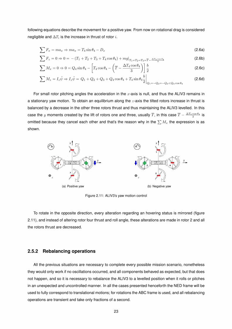
following equations describe the movement for a positive yaw. From now on rotational drag is considered

negligible and ∆Ti is the increase in thrust of rotor i.

∑Fx = max ⇒ max = T4 sin θ4 −Dx (2.6a)∑Fz = 0⇒ 0 = − (T1 + T2 + T3 + T4 cos θ4) +mg|

T1=T2=T3=T−∆T4 cos θ43

(2.6b)∑Mx = 0⇒ 0 = Q4 sin θ4 −

[T4 cos θ4 −

(T − ∆T4 cos θ4

3

)]b

2(2.6c)∑

Mz = Izψ ⇒ Izψ = Q1 +Q2 +Q3 +Q4 cos θ4 + T4 sin θ4b

2

∣∣∣∣Q1=−Q2=−Q3<Q4 cos θ4

(2.6d)

For small rotor pitching angles the acceleration in the x-axis is null, and thus the ALIV3 remains in

a stationary yaw motion. To obtain an equilibrium along the z-axis the tilted rotors increase in thrust is

balanced by a decrease in the other three rotors thrust and thus maintaining the ALIV3 levelled. In this

case the y moments created by the lift of rotors one and three, usually T , in this case T − ∆T4 cos θ43 is

omitted because they cancel each other and that’s the reason why in the∑Mx the expression is as

shown.

(a) Positive yaw (b) Negative yaw

Figure 2.11: ALIV3’s yaw motion control

To rotate in the opposite direction, every alteration regarding an hovering status is mirrored (figure

2.11), and instead of altering rotor four thrust and roll angle, these alterations are made in rotor 2 and all

the rotors thrust are decreased.

2.5.2 Rebalancing operations

All the previous situations are necessary to complete every possible mission scenario, nonetheless

they would only work if no oscillations occurred, and all components behaved as expected, but that does

not happen, and so it is necessary to rebalance the ALIV3 to a levelled position when it rolls or pitches

in an unexpected and uncontrolled manner. In all the cases presented henceforth the NED frame will be

used to fully correspond to translational motions; for rotations the ABC frame is used, and all rebalancing

operations are transient and take only fractions of a second.

23

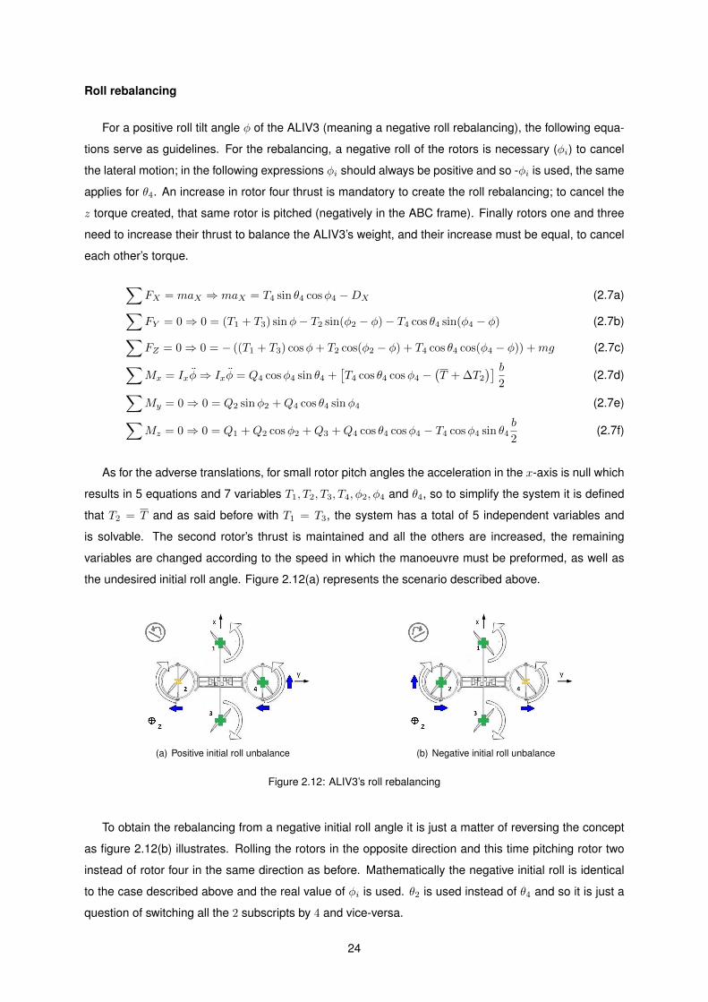
Roll rebalancing

For a positive roll tilt angle φ of the ALIV3 (meaning a negative roll rebalancing), the following equa-

tions serve as guidelines. For the rebalancing, a negative roll of the rotors is necessary (φi) to cancel

the lateral motion; in the following expressions φi should always be positive and so -φi is used, the same

applies for θ4. An increase in rotor four thrust is mandatory to create the roll rebalancing; to cancel the

z torque created, that same rotor is pitched (negatively in the ABC frame). Finally rotors one and three

need to increase their thrust to balance the ALIV3’s weight, and their increase must be equal, to cancel

each other’s torque.

∑FX = maX ⇒ maX = T4 sin θ4 cosφ4 −DX (2.7a)∑FY = 0⇒ 0 = (T1 + T3) sinφ− T2 sin(φ2 − φ)− T4 cos θ4 sin(φ4 − φ) (2.7b)∑FZ = 0⇒ 0 = − ((T1 + T3) cosφ+ T2 cos(φ2 − φ) + T4 cos θ4 cos(φ4 − φ)) +mg (2.7c)∑Mx = Ixφ⇒ Ixφ = Q4 cosφ4 sin θ4 +

[T4 cos θ4 cosφ4 −

(T + ∆T2

)] b2

(2.7d)∑My = 0⇒ 0 = Q2 sinφ2 +Q4 cos θ4 sinφ4 (2.7e)∑Mz = 0⇒ 0 = Q1 +Q2 cosφ2 +Q3 +Q4 cos θ4 cosφ4 − T4 cosφ4 sin θ4

b

2(2.7f)

As for the adverse translations, for small rotor pitch angles the acceleration in the x-axis is null which

results in 5 equations and 7 variables T1, T2, T3, T4, φ2, φ4 and θ4, so to simplify the system it is defined

that T2 = T and as said before with T1 = T3, the system has a total of 5 independent variables and

is solvable. The second rotor’s thrust is maintained and all the others are increased, the remaining

variables are changed according to the speed in which the manoeuvre must be preformed, as well as

the undesired initial roll angle. Figure 2.12(a) represents the scenario described above.

(a) Positive initial roll unbalance (b) Negative initial roll unbalance

Figure 2.12: ALIV3’s roll rebalancing

To obtain the rebalancing from a negative initial roll angle it is just a matter of reversing the concept

as figure 2.12(b) illustrates. Rolling the rotors in the opposite direction and this time pitching rotor two

instead of rotor four in the same direction as before. Mathematically the negative initial roll is identical

to the case described above and the real value of φi is used. θ2 is used instead of θ4 and so it is just a

question of switching all the 2 subscripts by 4 and vice-versa.

24

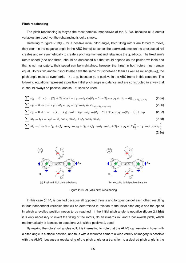
Pitch rebalancing

The pitch rebalancing is maybe the most complex manoeuvre of the ALIV3, because all 8 output

variables are used, yet the rebalancing is quite simple.

Referring to figure 2.13(a), for a positive initial pitch angle, both tilting rotors are forced to move,

they pitch (in the negative angle in the ABC frame) to cancel the backwards motion the unexpected roll

creates and roll symmetrically to create a pitching moment and rebalance the quadrotor. The fixed arm’s

rotors speed (one and three) should be decreased but that would depend on the power available and

that is not mandatory, their speed can be maintained, however the thrust in both rotors must remain

equal. Rotors two and four should also have the same thrust between them as well as roll angle (θi), the

pitch angle must be symmetric, −φ2 = φ4 because φ4 is positive in the ABC frame in this situation. The

following equations represent a positive initial pitch angle unbalance and are constructed in a way that

θi should always be positive, and so −θi shall be used.

∑FX = 0⇒ 0 = (T1 + T3) sin θ − T2 cosφ2 sin(θ2 − θ)− T2 cosφ4 sin(θ4 − θ)|T1=T3,T2=T4

(2.8a)∑FY = 0⇒ 0 = T2 cos θ2 sinφ2 − T4 cos θ4 sinφ4|θ2=θ4,−φ2=φ4

(2.8b)∑FZ = 0⇒ 0 = − ((T1 + T3) cos θ + T2 cosφ2 cos(θ2 − θ) + T4 cosφ4 cos(θ4 − θ)) +mg (2.8c)∑My = Iy θ ⇒ Iy θ = Q2 cos θ2 sinφ2 +Q4 cos θ4 sinφ4 (2.8d)∑Mz = 0⇒ 0 = Q1 +Q2 cos θ2 cosφ2 +Q3 +Q4 cos θ4 cosφ4 + T2 cosφ2 sin θ2

b

2− T4 cosφ4 sin θ4

b

2

(2.8e)

(a) Positive initial pitch unbalance (b) Negative initial pitch unbalance

Figure 2.13: ALIV3’s pitch rebalancing

In this case∑Mx is omitted because all opposed thrusts and torques cancel each other, resulting

in four independent variables that will be determined in relation to the initial pitch angle and the speed

in which a levelled position needs to be reached. If the initial pitch angle is negative (figure 2.13(b))

it is only necessary to invert the tilting of the rotors, do an inwards roll and a backwards pitch, which

mathematically is identical to equations 2.8, with a positive θi used.

By making the rotors’ roll angles null, it is interesting to note that the ALIV3 can remain in hover with

a pitch angle in a stable position, and thus with a mounted camera a wide variety of imagery is possible

with the ALIV3, because a rebalancing of the pitch angle or a transition to a desired pitch angle is the

25

same operation, and then to remain in hover in that position, is just a case of making all equations in

2.8 equal zero by imposing φ2 = φ4 = 0 and thus the global pitch angle φ is maintained and the ALIV3

maintains its position.

2.5.3 Combined motions

Up until now all possible motions were only shown isolated, however in a real flight situation more

than one of the described manoeuvres may need to be executed at the same time, and that can be

done simply by combining the wanted motions simultaneously. In the previous rebalancing subsection

the autonomous ALIV3’s motions were described, those are the manoeuvres that the control should be

responsible for, without any interference from the pilot, and should activate immediately when necessary,

to rebalance the ALIV3.

In subsection 2.5.1 (levelled motions) the motions described were supposed to be controlled by the

user, yet all of those motions are subjected to oscillations and so the control software needs to be

aware of what the motion, or motions, the pilot desires and disable all other, applying the necessary

compensations in case of unwanted and unexpected oscillations both for translations as for rotations.

26

Chapter 3

Rotor Optimization

One of the key components of every quadrotor are its rotors, responsible for the transmission of

the motor’s power to the air and subsequently responsible for the force production in the aircraft, to

counteract its weight or to move it through the air. In our case the rotors are fixed to the motors and

do not need additional degrees of freedom in that connection, they just need to produce a lifting force

in the motor’s direction. A wide variety of rotor options are available in the market, but usually only for

right-hand rotation, to serve as an airplane’s propeller. The nomenclature difference is based on historic

reasons, where a propeller is solely responsible for the production of horizontal thrust, where a rotor is

usually responsible for the lifting of helicopters but latter adapted to moving propeller with the inception

of tiltrotors.

In every quadrotor right-hand (pusher) and left-hand (puller) propellers are necessary due to the

torque cancellation requisite, but the market does not provide a wide variety of puller options, and so the

creation of an optimum rotor for the ALIV3 is an interesting and challenging alternative. In Pedro’s work

[18] a Genetic Algorithm (GA) implemented in Octave based on the Blade Element Momentum Theory

(BEMT) was created to preform this task, and in this chapter an improved version, this time in MatLab R©,

of this solution will be presented since Pedro’s alternative had a few problems that needed revision, and

an improved code was necessary to create a new de facto optimum rotor for the ALIV3.

A few aspects are of major importance for the optimum rotor creation, such as the selection of

the perfect aerofoil for the situation at hand, choosing a rotor theory to estimate the rotor’s behaviour

and finally assemble the genetic algorithm to determine the maximum of the function coming from the

selected rotor theory. The theoretical principles behind these aspects need to be presented first.

3.1 Theoretical principles

3.1.1 Panel Method

To analyse what aerofoil should be selected for an ideal rotor the Computational Fluid Dynamics

(CFD) XFLR51 program will be used. The XFLR5 is the evolution of the two-dimensional panel method1http://xflr5.sourceforge.net/xflr5.htm

27

implementation by Drela, 1989 [27] in his XFOIL which was an interactive program that utilized a two-

dimensional panel method code with integral boundary layer theory to analyse aerofoils in viscous or

inviscid flow fields.

The origins of the panel method date back to 1967 when a three-dimensional panel method was

introduced to estimate the drag of a ship hull [28]. After that all the major aerospace companies devel-

oped their own kind of programmes, meanwhile the two-dimensional realm also evolved and a number

of panel method codes have been developed for aerofoil analysis and design. The panel method codes

with more acknowledgement are Professor Richard Eppler’s (of the University of Stuttgart) PROFIL code,

developed partly funded by NASA, in the early 1980s, and MIT Professor Mark Drela’s XFOIL code, the

one that served as base for XFLR5 used in this thesis.

The viscous formulation [29] which is the one used in XFLR5, is ruled by the following standard

compressible integral momentum and kinetic energy shape parameter equations, where the streamwise

coordinate is ξ.dθ

dξ+ (2 +H −M2

ae)θ

Ve

dVedξ

=Cf2

(3.1)

θdH∗

dξ+ (2H∗∗ +H∗(1−H))

θ

Ve

dVedξ

= 2Cd −H∗Cf2

(3.2)

Being V the velocity, Ma the Mach number, Cf the skin-friction coefficient equal to 2τwall/ρeV2e , with

τwall as the shear stress of the wall and ρ as the density. The subscript e refers to the boundary-layer

edge. The momentum thickness θ is given by∫ (

ρVρeVe

) [1−

(VVe

)]dη where η is the perpendicular

direction to ξ on the aerofoil plane. The shape parameter is H = δ∗

θ with δ as the boundary layer

thickness and δ∗ as the displacement thickness δ∗ =∫ [

1−(ρVρeVe

)]dη. Finally Hk is the kinematic

shape parameter equal to∫

[1− (V/Ve)]dη/∫

(V/Ve)[1− (V/Ve)]dη. H∗ is defined as the kinetic energy

shape parameter (H∗ = θ∗/θ) and H∗∗ the density shape parameter, defined by δ∗∗/θ, where δ∗∗ is the

density thickness∫

(V/Ve)[1− (ρ/ρe)]dη and θ∗ the kinetic energy thickness∫

(ρV/ρeVe)[1− (V/Ve)2]dη.

A rate equation for the maximum shear stress coefficient (Cτ ) is used to account for deviations of the

outer layer dissipation coefficient (Cd = (1/ρeV3e )∫τ(∂V/∂η)dη) from the local equilibrium value, known

as the shear stress lag equation, however in this case it is only important to consider laminar cases

(Re < 5 × 105) [30], since the Reynolds number (Re = V c/ν) for the rotor size in study (in table 3.2

Re ' 35000) is very low, the value of the rotor cord (c) is very small, (whereas ν is the kinematic viscosity

of the air) and so the stress lag equation is substituted by:

dn

dξ=

dn

dReθ(Hk)

dReθdξ

(Hk, θ) (3.3)

that models the growth of amplitude in n (transition disturbance amplification variable) of the most

amplified Tollmien-Schlichting wave, with Reθ as the momentum thickness Reynolds number equal to

ρeVeδ/µe and µ as the dynamic viscosity.

Using θ, δ∗ and n as governing variables and using equations 3.1, 3.2, 3.3 and adding Ve, as an

external unknown that does not constitute an additional system unknown it is just a matter of discretizing

those equations using two-point central differences, e.g. the trapezoidal rule, to create a non-linear

28

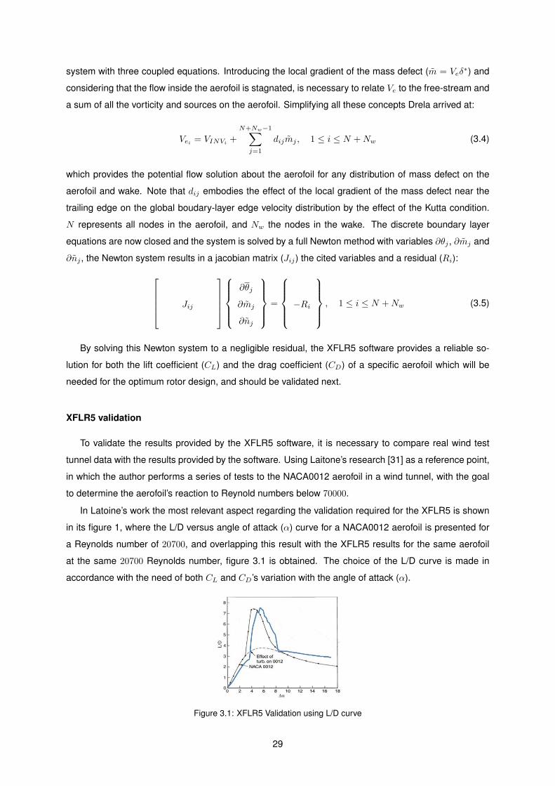
system with three coupled equations. Introducing the local gradient of the mass defect (m = Veδ∗) and

considering that the flow inside the aerofoil is stagnated, is necessary to relate Ve to the free-stream and

a sum of all the vorticity and sources on the aerofoil. Simplifying all these concepts Drela arrived at:

Vei = VINVi +

N+Nw−1∑j=1

dijmj , 1 ≤ i ≤ N +Nw (3.4)

which provides the potential flow solution about the aerofoil for any distribution of mass defect on the

aerofoil and wake. Note that dij embodies the effect of the local gradient of the mass defect near the

trailing edge on the global boudary-layer edge velocity distribution by the effect of the Kutta condition.

N represents all nodes in the aerofoil, and Nw the nodes in the wake. The discrete boundary layer

equations are now closed and the system is solved by a full Newton method with variables ∂θj , ∂mj and

∂nj , the Newton system results in a jacobian matrix (Jij) the cited variables and a residual (Ri): Jij

∂θj

∂mj

∂nj

=

−Ri , 1 ≤ i ≤ N +Nw (3.5)

By solving this Newton system to a negligible residual, the XFLR5 software provides a reliable so-

lution for both the lift coefficient (CL) and the drag coefficient (CD) of a specific aerofoil which will be

needed for the optimum rotor design, and should be validated next.

XFLR5 validation

To validate the results provided by the XFLR5 software, it is necessary to compare real wind test

tunnel data with the results provided by the software. Using Laitone’s research [31] as a reference point,

in which the author performs a series of tests to the NACA0012 aerofoil in a wind tunnel, with the goal

to determine the aerofoil’s reaction to Reynold numbers below 70000.

In Latoine’s work the most relevant aspect regarding the validation required for the XFLR5 is shown

in its figure 1, where the L/D versus angle of attack (α) curve for a NACA0012 aerofoil is presented for

a Reynolds number of 20700, and overlapping this result with the XFLR5 results for the same aerofoil

at the same 20700 Reynolds number, figure 3.1 is obtained. The choice of the L/D curve is made in

accordance with the need of both CL and CD ’s variation with the angle of attack (α).

Figure 3.1: XFLR5 Validation using L/D curve

29

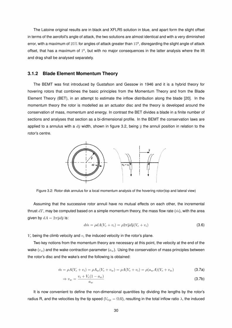
The Latoine original results are in black and XFLR5 solution in blue, and apart form the slight offset

in terms of the aerofoil’s angle of attack, the two solutions are almost identical and with a very diminished

error, with a maximum of 25% for angles of attack greater than 15o, disregarding the slight angle of attack

offset, that has a maximum of 1o, but with no major consequences in the latter analysis where the lift

and drag shall be analysed separately.

3.1.2 Blade Element Momentum Theory

The BEMT was first introduced by Gustafson and Gessow in 1946 and it is a hybrid theory for

hovering rotors that combines the basic principles from the Momentum Theory and from the Blade

Element Theory (BET), in an attempt to estimate the inflow distribution along the blade [20]. In the

momentum theory the rotor is modelled as an actuator disc and the theory is developed around the

conservation of mass, momentum and energy. In contrast the BET divides a blade in a finite number of

sections and analyses that section as a bi-dimensional profile. In the BEMT the conservation laws are

applied to a annulus with a dy width, shown in figure 3.2, being y the annuli position in relation to the

rotor’s centre.

Figure 3.2: Rotor disk annulus for a local momentum analysis of the hovering rotor(top and lateral view)

Assuming that the successive rotor annuli have no mutual effects on each other, the incremental

thrust dT , may be computed based on a simple momentum theory, the mass flow rate (m), with the area

given by dA = 2πydy is:

dm = ρdA(Vc + vi) = ρ2πydy(Vc + vi) (3.6)

Vc being the climb velocity and vi the induced velocity in the rotor’s plane.

Two key notions from the momentum theory are necessary at this point, the velocity at the end of the

wake (vw) and the wake contraction parameter (aw). Using the conservation of mass principles between

the rotor’s disc and the wake’s end the following is obtained:

m = ρA(Vc + vi) = ρAw(Vc + vw) = ρA(Vc + vi) = ρ(awA)(Vc + vw) (3.7a)

⇒ vw =vi + Vc(1− aw)

aw(3.7b)

It is now convenient to define the non-dimensional quantities by dividing the lengths by the rotor’s

radius R, and the velocities by the tip speed (Vtip = ΩR), resulting in the total inflow ratio λ, the induced

30

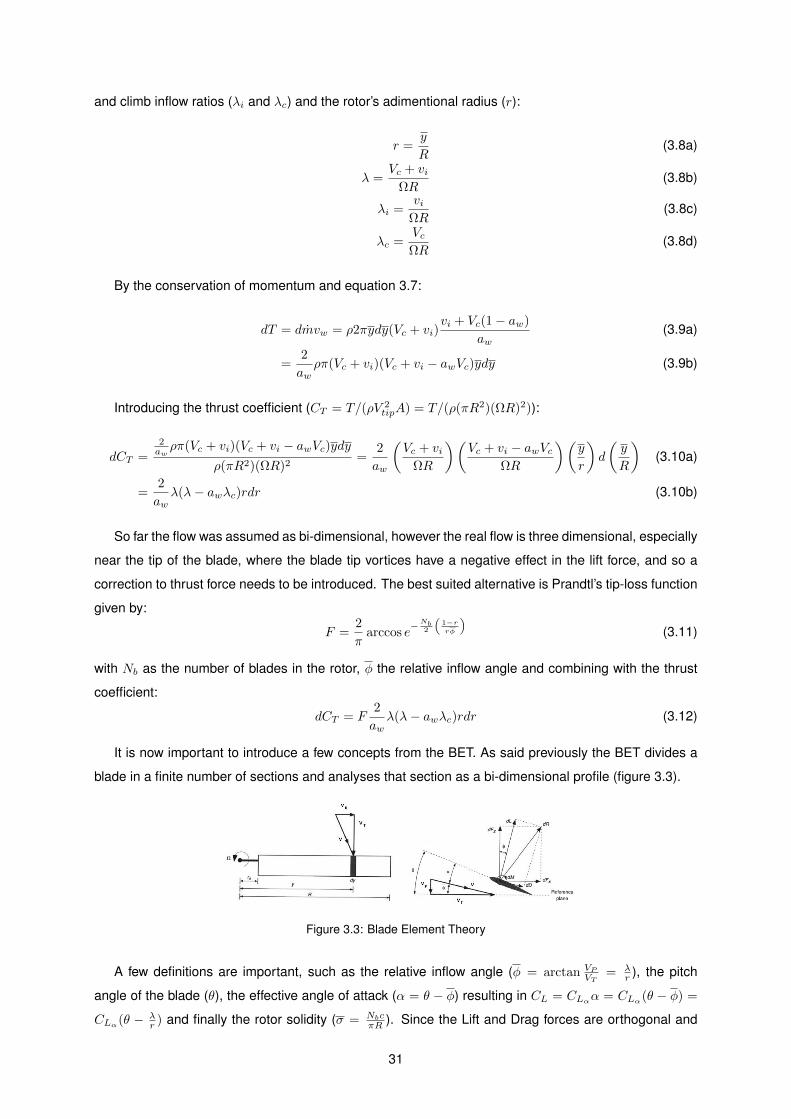
and climb inflow ratios (λi and λc) and the rotor’s adimentional radius (r):

r =y

R(3.8a)

λ =Vc + vi

ΩR(3.8b)

λi =vi

ΩR(3.8c)

λc =VcΩR

(3.8d)

By the conservation of momentum and equation 3.7:

dT = dmvw = ρ2πydy(Vc + vi)vi + Vc(1− aw)

aw(3.9a)

=2

awρπ(Vc + vi)(Vc + vi − awVc)ydy (3.9b)

Introducing the thrust coefficient (CT = T/(ρV 2tipA) = T/(ρ(πR2)(ΩR)2)):

dCT =2awρπ(Vc + vi)(Vc + vi − awVc)ydy

ρ(πR2)(ΩR)2=

2

aw

(Vc + vi

ΩR

)(Vc + vi − awVc

ΩR

)(y

r

)d

(y

R

)(3.10a)

=2

awλ(λ− awλc)rdr (3.10b)

So far the flow was assumed as bi-dimensional, however the real flow is three dimensional, especially

near the tip of the blade, where the blade tip vortices have a negative effect in the lift force, and so a

correction to thrust force needs to be introduced. The best suited alternative is Prandtl’s tip-loss function

given by:

F =2

πarccos e

−Nb2(

1−rrφ

)(3.11)

with Nb as the number of blades in the rotor, φ the relative inflow angle and combining with the thrust

coefficient:

dCT = F2

awλ(λ− awλc)rdr (3.12)

It is now important to introduce a few concepts from the BET. As said previously the BET divides a

blade in a finite number of sections and analyses that section as a bi-dimensional profile (figure 3.3).

Figure 3.3: Blade Element Theory

A few definitions are important, such as the relative inflow angle (φ = arctan VPVT

= λr ), the pitch

angle of the blade (θ), the effective angle of attack (α = θ − φ) resulting in CL = CLαα = CLα(θ − φ) =

CLα(θ − λr ) and finally the rotor solidity (σ = Nbc

πR ). Since the Lift and Drag forces are orthogonal and

31

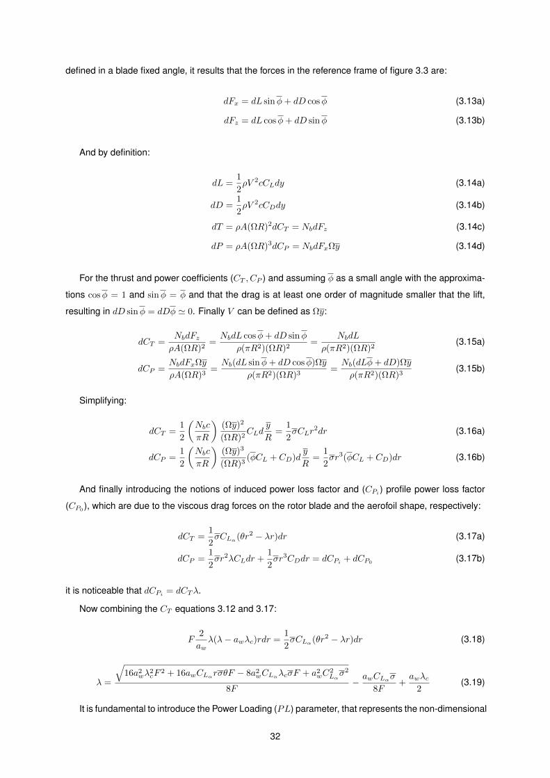
defined in a blade fixed angle, it results that the forces in the reference frame of figure 3.3 are:

dFx = dL sinφ+ dD cosφ (3.13a)

dFz = dL cosφ+ dD sinφ (3.13b)

And by definition:

dL =1

2ρV 2cCLdy (3.14a)

dD =1

2ρV 2cCDdy (3.14b)

dT = ρA(ΩR)2dCT = NbdFz (3.14c)

dP = ρA(ΩR)3dCP = NbdFxΩy (3.14d)

For the thrust and power coefficients (CT , CP ) and assuming φ as a small angle with the approxima-

tions cosφ = 1 and sinφ = φ and that the drag is at least one order of magnitude smaller that the lift,

resulting in dD sinφ = dDφ ' 0. Finally V can be defined as Ωy:

dCT =NbdFzρA(ΩR)2

=NbdL cosφ+ dD sinφ

ρ(πR2)(ΩR)2=

NbdL

ρ(πR2)(ΩR)2(3.15a)

dCP =NbdFxΩy

ρA(ΩR)3=Nb(dL sinφ+ dD cosφ)Ωy

ρ(πR2)(ΩR)3=Nb(dLφ+ dD)Ωy

ρ(πR2)(ΩR)3(3.15b)

Simplifying:

dCT =1

2

(Nbc

πR

)(Ωy)2

(ΩR)2CLd

y

R=

1

2σCLr

2dr (3.16a)

dCP =1

2

(Nbc

πR

)(Ωy)3

(ΩR)3(φCL + CD)d

y

R=

1

2σr3(φCL + CD)dr (3.16b)

And finally introducing the notions of induced power loss factor and (CPi ) profile power loss factor

(CP0 ), which are due to the viscous drag forces on the rotor blade and the aerofoil shape, respectively:

dCT =1

2σCLα(θr2 − λr)dr (3.17a)

dCP =1

2σr2λCLdr +

1

2σr3CDdr = dCPi + dCP0 (3.17b)

it is noticeable that dCPi = dCTλ.

Now combining the CT equations 3.12 and 3.17:

F2

awλ(λ− awλc)rdr =

1

2σCLα(θr2 − λr)dr (3.18)

λ =

√16a2

wλ2cF

2 + 16awCLαrσθF − 8a2wCLαλcσF + a2

wC2Lασ2

8F− awCLασ

8F+awλc

2(3.19)

It is fundamental to introduce the Power Loading (PL) parameter, that represents the non-dimensional

32

ratio of thrust produced to the power required and is the variable to maximize in the GA implementation

to achieve the optimum rotor:

PL =T

P=W

P=

CTCP (ΩR)

(3.20)

BEMT implementation

Based on the previous equations, and with CT calculated from eq.3.17, the BEMT code is con-

structed. However it is noticeable that CT and CP depend on λ, CL and CD, that depends of F and α,

that are dependent of φ that depend on λ and so an iterative process is required to achieve a solution.

In Pedro’s work [18] a BEMT code was created, however some key aspects were approximated,

and no iterative process was implemented. The major shortcomings were the non-implementation of

the tip-loss factor, assuming the flow along the rotor disc as perfectly two dimensional, the other major

drawback was the approximation of CL = 2πα which is valid for high Reynolds numbers (i.e. 1 × 105)

and angles of attack below 10o for symmetric aerofoils. It is important to determine, for small scale

rotors, what is the magnitude of the Reynolds numbers in place, so considering the following properties

achieved by Pedro in his optimum rotor estimation:

Average Properties

ρ 1.225kg.m−3

µ 1.8× 10−5kg.m−1.s−1

V = Ωy 60m.s−1

c 8.5mm

Re = ρV cµ 34708.3

Table 3.1: Reynolds related properties for small rotors

And so for the real situation presented, the average Reynolds number magnitude is one order of

magnitude smaller than the validity of the CL approximation. To confirm this aspect in figure 3.4 is shown

how the lift coefficient versus α behaves, varying the Reynolds number for the NACA0012 aerofoil:

Figure 3.4: NACA0012 CL versus α for a range of Reynolds numbers

Analysing figure 3.4 it is confirmed that the CL values should be taken into consideration to a thor-

ough and correct implementation of the BEMT theory. For a Reynolds number of 35000 the linear

CL = 2πα approximation is valid for an angle below 8o. This could mean that for angles below 8o

33

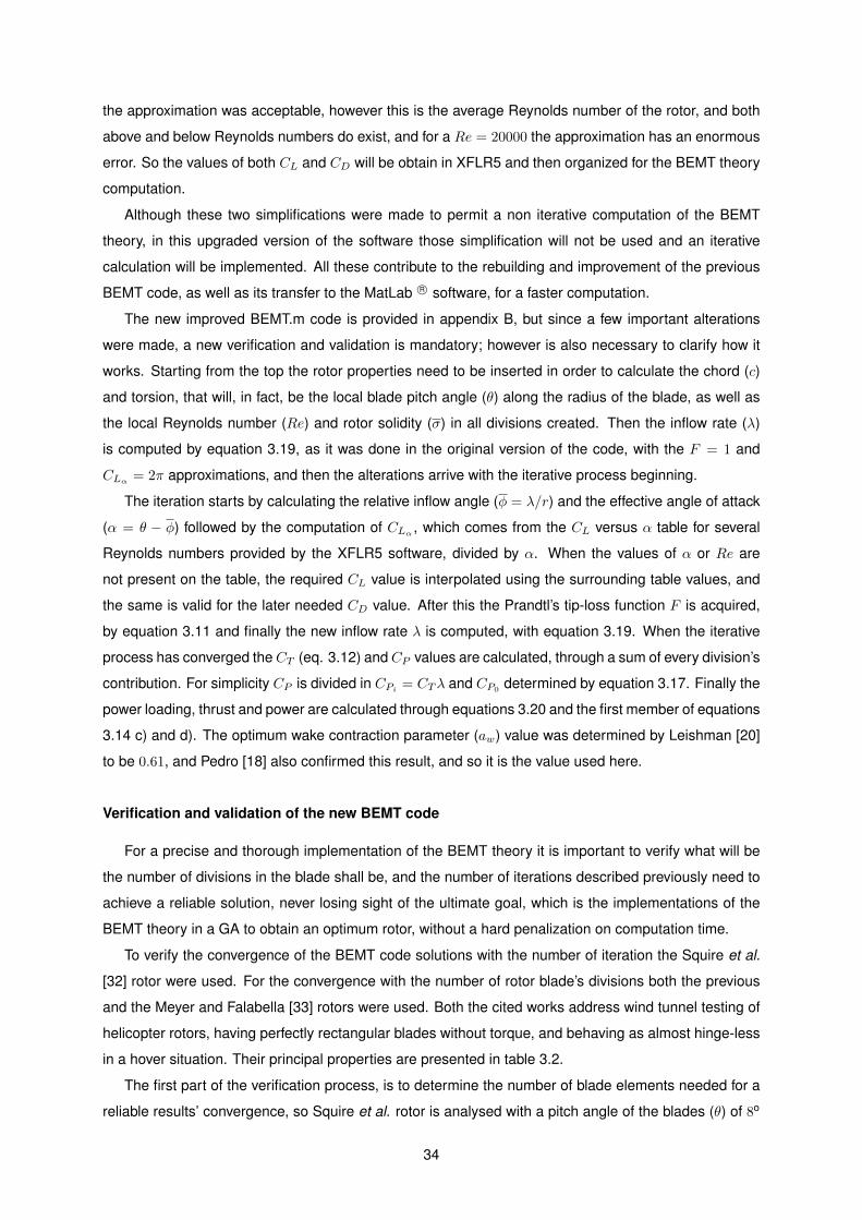
the approximation was acceptable, however this is the average Reynolds number of the rotor, and both

above and below Reynolds numbers do exist, and for a Re = 20000 the approximation has an enormous

error. So the values of both CL and CD will be obtain in XFLR5 and then organized for the BEMT theory

computation.

Although these two simplifications were made to permit a non iterative computation of the BEMT

theory, in this upgraded version of the software those simplification will not be used and an iterative

calculation will be implemented. All these contribute to the rebuilding and improvement of the previous

BEMT code, as well as its transfer to the MatLab R© software, for a faster computation.

The new improved BEMT.m code is provided in appendix B, but since a few important alterations

were made, a new verification and validation is mandatory; however is also necessary to clarify how it

works. Starting from the top the rotor properties need to be inserted in order to calculate the chord (c)

and torsion, that will, in fact, be the local blade pitch angle (θ) along the radius of the blade, as well as

the local Reynolds number (Re) and rotor solidity (σ) in all divisions created. Then the inflow rate (λ)

is computed by equation 3.19, as it was done in the original version of the code, with the F = 1 and

CLα = 2π approximations, and then the alterations arrive with the iterative process beginning.

The iteration starts by calculating the relative inflow angle (φ = λ/r) and the effective angle of attack

(α = θ − φ) followed by the computation of CLα , which comes from the CL versus α table for several

Reynolds numbers provided by the XFLR5 software, divided by α. When the values of α or Re are

not present on the table, the required CL value is interpolated using the surrounding table values, and

the same is valid for the later needed CD value. After this the Prandtl’s tip-loss function F is acquired,

by equation 3.11 and finally the new inflow rate λ is computed, with equation 3.19. When the iterative

process has converged the CT (eq. 3.12) and CP values are calculated, through a sum of every division’s

contribution. For simplicity CP is divided in CPi = CTλ and CP0determined by equation 3.17. Finally the

power loading, thrust and power are calculated through equations 3.20 and the first member of equations

3.14 c) and d). The optimum wake contraction parameter (aw) value was determined by Leishman [20]

to be 0.61, and Pedro [18] also confirmed this result, and so it is the value used here.

Verification and validation of the new BEMT code

For a precise and thorough implementation of the BEMT theory it is important to verify what will be

the number of divisions in the blade shall be, and the number of iterations described previously need to

achieve a reliable solution, never losing sight of the ultimate goal, which is the implementations of the

BEMT theory in a GA to obtain an optimum rotor, without a hard penalization on computation time.

To verify the convergence of the BEMT code solutions with the number of iteration the Squire et al.

[32] rotor were used. For the convergence with the number of rotor blade’s divisions both the previous

and the Meyer and Falabella [33] rotors were used. Both the cited works address wind tunnel testing of

helicopter rotors, having perfectly rectangular blades without torque, and behaving as almost hinge-less

in a hover situation. Their principal properties are presented in table 3.2.

The first part of the verification process, is to determine the number of blade elements needed for a

reliable results’ convergence, so Squire et al. rotor is analysed with a pitch angle of the blades (θ) of 8o

34

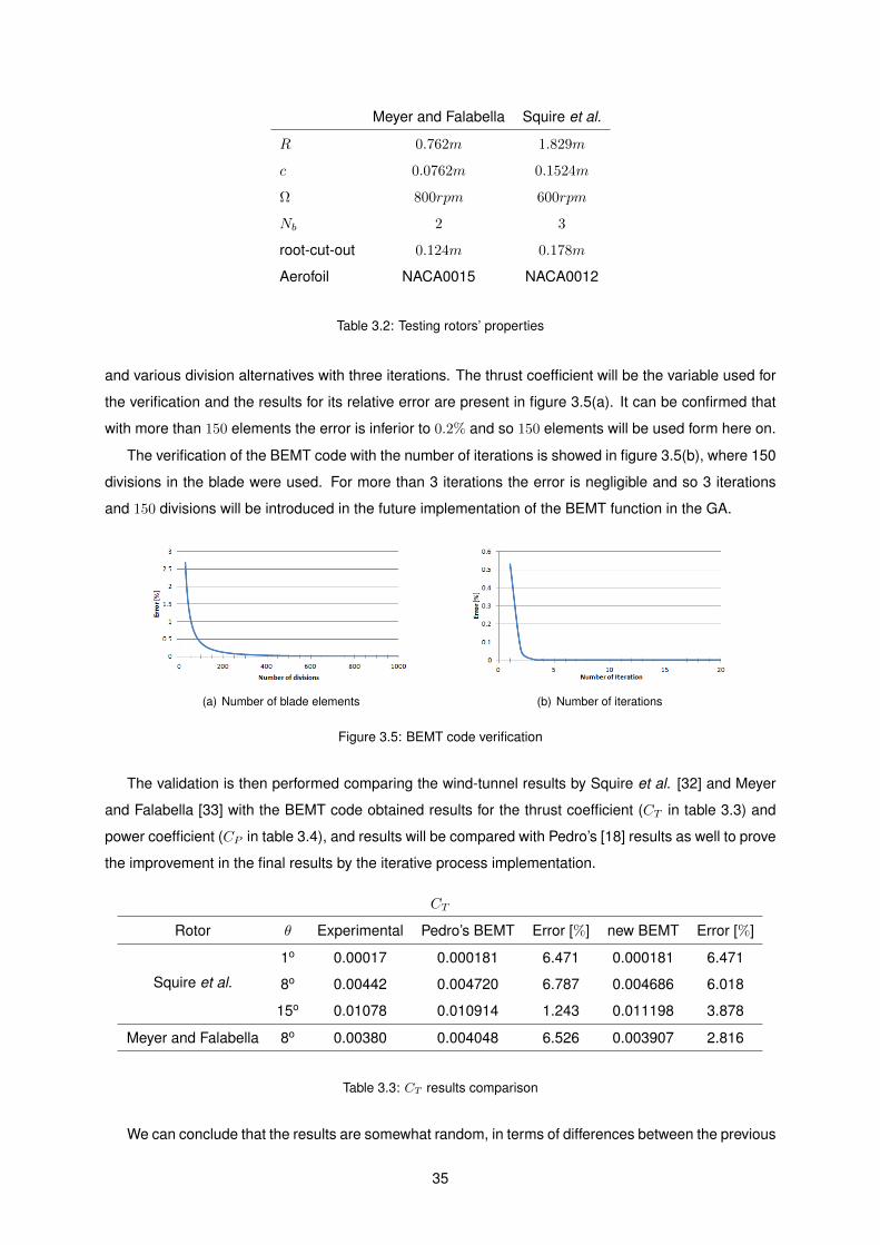
Meyer and Falabella Squire et al.

R 0.762m 1.829m

c 0.0762m 0.1524m

Ω 800rpm 600rpm

Nb 2 3

root-cut-out 0.124m 0.178m

Aerofoil NACA0015 NACA0012

Table 3.2: Testing rotors’ properties

and various division alternatives with three iterations. The thrust coefficient will be the variable used for

the verification and the results for its relative error are present in figure 3.5(a). It can be confirmed that

with more than 150 elements the error is inferior to 0.2% and so 150 elements will be used form here on.

The verification of the BEMT code with the number of iterations is showed in figure 3.5(b), where 150

divisions in the blade were used. For more than 3 iterations the error is negligible and so 3 iterations

and 150 divisions will be introduced in the future implementation of the BEMT function in the GA.

(a) Number of blade elements (b) Number of iterations

Figure 3.5: BEMT code verification

The validation is then performed comparing the wind-tunnel results by Squire et al. [32] and Meyer

and Falabella [33] with the BEMT code obtained results for the thrust coefficient (CT in table 3.3) and

power coefficient (CP in table 3.4), and results will be compared with Pedro’s [18] results as well to prove

the improvement in the final results by the iterative process implementation.

CT

Rotor θ Experimental Pedro’s BEMT Error [%] new BEMT Error [%]

Squire et al.

1o 0.00017 0.000181 6.471 0.000181 6.471

8o 0.00442 0.004720 6.787 0.004686 6.018

15o 0.01078 0.010914 1.243 0.011198 3.878

Meyer and Falabella 8o 0.00380 0.004048 6.526 0.003907 2.816

Table 3.3: CT results comparison

We can conclude that the results are somewhat random, in terms of differences between the previous

35

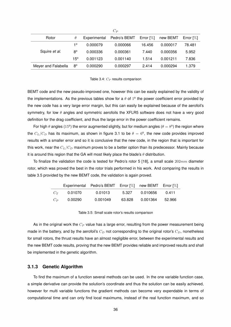
CP

Rotor θ Experimental Pedro’s BEMT Error [%] new BEMT Error [%]

Squire et al.

1o 0.000079 0.000066 16.456 0.000017 78.481

8o 0.000336 0.000361 7.440 0.000356 5.952

15o 0.001123 0.001140 1.514 0.001211 7.836

Meyer and Falabella 8o 0.000290 0.000297 2.414 0.000294 1.379

Table 3.4: CP results comparison

BEMT code and the new pseudo-improved one, however this can be easily explained by the validity of

the implementations. As the previous tables show for a θ of 1o the power coefficient error provided by

the new code has a very large error margin, but this can easily be explained because of the aerofoil’s

symmetry, for low θ angles and symmetric aerofoils the XFLR5 software does not have a very good

definition for the drag coefficient, and thus the large error in the power coefficient remains.

For high θ angles (15o) the error augmented slightly, but for medium angles (θ = 8o) the region where

the CL/CD has its maximum, as shown in figure 3.1 to be θ = 6o, the new code provides improved

results with a smaller error and so it is conclusive that the new code, in the region that is important for

this work, near the CL/CD maximum proves to be a better option than its predecessor. Mainly because

it is around this region that the GA will most likely place the blade’s θ distribution.

To finalize the validation the code is tested for Pedro’s rotor 5 [18], a small scale 202mm diameter

rotor, which was proved the best in the rotor trials performed in his work. And comparing the results in

table 3.5 provided by the new BEMT code, the validation is again proved.

Experimental Pedro’s BEMT Error [%] new BEMT Error [%]

CT 0.01070 0.01013 5.327 0.010656 0.411

CP 0.00290 0.001049 63.828 0.001364 52.966

Table 3.5: Small scale rotor’s results comparison

As in the original work the CP value has a large error, resulting from the power measurement being

made in the battery, and by the aerofoil’s CD not corresponding to the original rotor’s CD, nonetheless

for small rotors, the thrust results have an almost negligible error, between the experimental results and

the new BEMT code results, proving that the new BEMT provides reliable and improved results and shall

be implemented in the genetic algorithm.

3.1.3 Genetic Algorithm

To find the maximum of a function several methods can be used. In the one variable function case,

a simple derivative can provide the solution’s coordinate and thus the solution can be easily achieved,

however for multi variable functions the gradient methods can become very expendable in terms of

computational time and can only find local maximums, instead of the real function maximum, and so

36

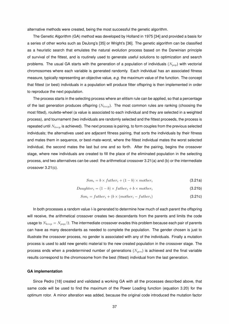
alternative methods were created, being the most successful the genetic algorithm.

The Genetic Algorithm (GA) method was developed by Holland in 1975 [34] and provided a basis for

a series of other works such as DeJong’s [35] or Wright’s [36]. The genetic algorithm can be classified

as a heuristic search that emulates the natural evolution process based on the Darwinian principle

of survival of the fittest, and is routinely used to generate useful solutions to optimization and search

problems. The usual GA starts with the generation of a population of individuals (Npop) with vectorial

chromosomes where each variable is generated randomly. Each individual has an associated fitness

measure, typically representing an objective value, e.g. the maximum value of the function. The concept

that fittest (or best) individuals in a population will produce fitter offspring is then implemented in order

to reproduce the next population.

The process starts in the selecting process where an elitism rule can be applied, so that a percentage

of the last generation produces offspring (Nkeep). The most common rules are ranking (choosing the

most fitted), roulette-wheel (a value is associated to each individual and they are selected in a weighted

process), and tournament (two individuals are randomly selected and the fittest proceeds, the process is

repeated untilNkeep is achieved). The next process is pairing, to form couples from the previous selected

individuals; the alternatives used are adjacent fitness pairing, that sorts the individuals by their fitness

and mates them in sequence, or best-mate-worst, where the fittest individual mates the worst selected

individual, the second mates the last but one and so forth. After the pairing, begins the crossover

stage, where new individuals are created to fill the place of the eliminated population in the selecting

process, and two alternatives can be used: the arithmetical crossover 3.21(a) and (b) or the intermediate

crossover 3.21(c).

Soni = b× fatheri + (1− b)×motheri (3.21a)

Daughteri = (1− b)× fatheri + b×motheri (3.21b)

Soni = fatheri + (b× (motheri − fatheri) (3.21c)

In both processes a random value b is generated to determine how much of each parent the offspring

will receive, the arithmetical crossover creates two descendants from the parents and limits the code

usage to Nkeep = Npop/2. The intermediate crossover evades this problem because each pair of parents

can have as many descendants as needed to complete the population. The gender chosen is just to

illustrate the crossover process, no gender is associated with any of the individuals. Finally a mutation

process is used to add new genetic material to the new created population in the crossover stage. The

process ends when a predetermined number of generations (Ngen) is achieved and the final variable

results correspond to the chromosome from the best (fittest) individual from the last generation.

GA implementation

Since Pedro [18] created and validated a working GA with all the processes described above, that

same code will be used to find the maximum of the Power Loading function (equation 3.20) for the

optimum rotor. A minor alteration was added, because the original code introduced the mutation factor

37

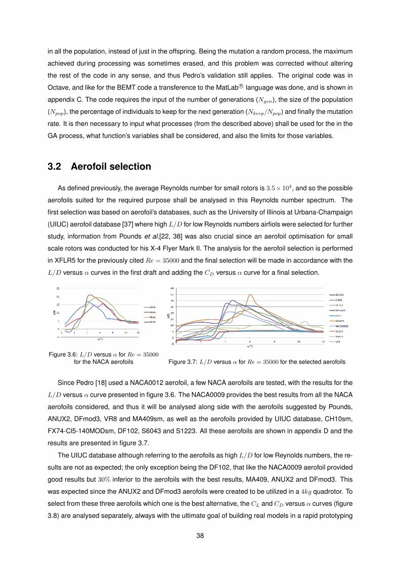
in all the population, instead of just in the offspring. Being the mutation a random process, the maximum

achieved during processing was sometimes erased, and this problem was corrected without altering

the rest of the code in any sense, and thus Pedro’s validation still applies. The original code was in

Octave, and like for the BEMT code a transference to the MatLab R© language was done, and is shown in

appendix C. The code requires the input of the number of generations (Ngen), the size of the population

(Npop), the percentage of individuals to keep for the next generation (Nkeep/Npop) and finally the mutation

rate. It is then necessary to input what processes (from the described above) shall be used for the in the

GA process, what function’s variables shall be considered, and also the limits for those variables.

3.2 Aerofoil selection

As defined previously, the average Reynolds number for small rotors is 3.5× 104, and so the possible

aerofoils suited for the required purpose shall be analysed in this Reynolds number spectrum. The

first selection was based on aerofoil’s databases, such as the University of Illinois at Urbana-Champaign

(UIUC) aerofoil database [37] where high L/D for low Reynolds numbers airfiols were selected for further

study, information from Pounds et al.[22, 38] was also crucial since an aerofoil optimisation for small

scale rotors was conducted for his X-4 Flyer Mark II. The analysis for the aerofoil selection is performed

in XFLR5 for the previously cited Re = 35000 and the final selection will be made in accordance with the

L/D versus α curves in the first draft and adding the CD versus α curve for a final selection.

Figure 3.6: L/D versus α for Re = 35000for the NACA aerofoils Figure 3.7: L/D versus α for Re = 35000 for the selected aerofoils

Since Pedro [18] used a NACA0012 aerofoil, a few NACA aerofoils are tested, with the results for the

L/D versus α curve presented in figure 3.6. The NACA0009 provides the best results from all the NACA

aerofoils considered, and thus it will be analysed along side with the aerofoils suggested by Pounds,

ANUX2, DFmod3, VR8 and MA409sm, as well as the aerofoils provided by UIUC database, CH10sm,

FX74-Cl5-140MODsm, DF102, S6043 and S1223. All these aerofoils are shown in appendix D and the

results are presented in figure 3.7.

The UIUC database although referring to the aerofoils as high L/D for low Reynolds numbers, the re-

sults are not as expected; the only exception being the DF102, that like the NACA0009 aerofoil provided

good results but 30% inferior to the aerofoils with the best results, MA409, ANUX2 and DFmod3. This

was expected since the ANUX2 and DFmod3 aerofoils were created to be utilized in a 4kg quadrotor. To

select from these three aerofoils which one is the best alternative, the CL and CD versus α curves (figure

3.8) are analysed separately, always with the ultimate goal of building real models in a rapid prototyping

38

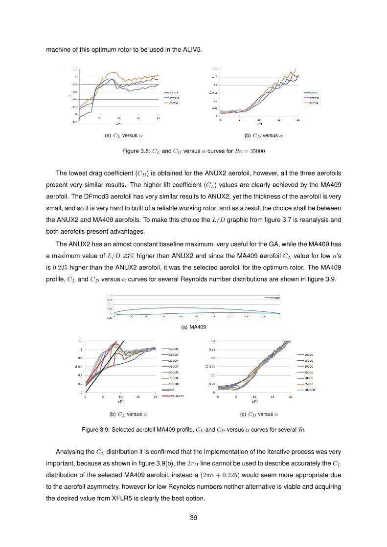
machine of this optimum rotor to be used in the ALIV3.

(a) CL versus α (b) CD versus α

Figure 3.8: CL and CD versus α curves for Re = 35000

The lowest drag coefficient (CD) is obtained for the ANUX2 aerofoil, however, all the three aerofoils

present very similar results. The higher lift coefficient (CL) values are clearly achieved by the MA409

aerofoil. The DFmod3 aerofoil has very similar results to ANUX2, yet the thickness of the aerofoil is very

small, and so it is very hard to built of a reliable working rotor, and as a result the choice shall be between

the ANUX2 and MA409 aerofoils. To make this choice the L/D graphic from figure 3.7 is reanalysis and

both aerofoils present advantages.

The ANUX2 has an almost constant baseline maximum, very useful for the GA, while the MA409 has

a maximum value of L/D 23% higher than ANUX2 and since the MA409 aerofoil CL value for low α’s

is 0.225 higher than the ANUX2 aerofoil, it was the selected aerofoil for the optimum rotor. The MA409

profile, CL and CD versus α curves for several Reynolds number distributions are shown in figure 3.9.

(a) MA409

(b) CL versus α (c) CD versus α

Figure 3.9: Selected aerofoil MA409 profile, CL and CD versus α curves for several Re

Analysing the CL distribution it is confirmed that the implementation of the iterative process was very

important, because as shown in figure 3.9(b), the 2πα line cannot be used to describe accurately the CL

distribution of the selected MA409 aerofoil, instead a (2πα + 0.225) would seem more appropriate due

to the aerofoil asymmetry, however for low Reynolds numbers neither alternative is viable and acquiring

the desired value from XFLR5 is clearly the best option.

39

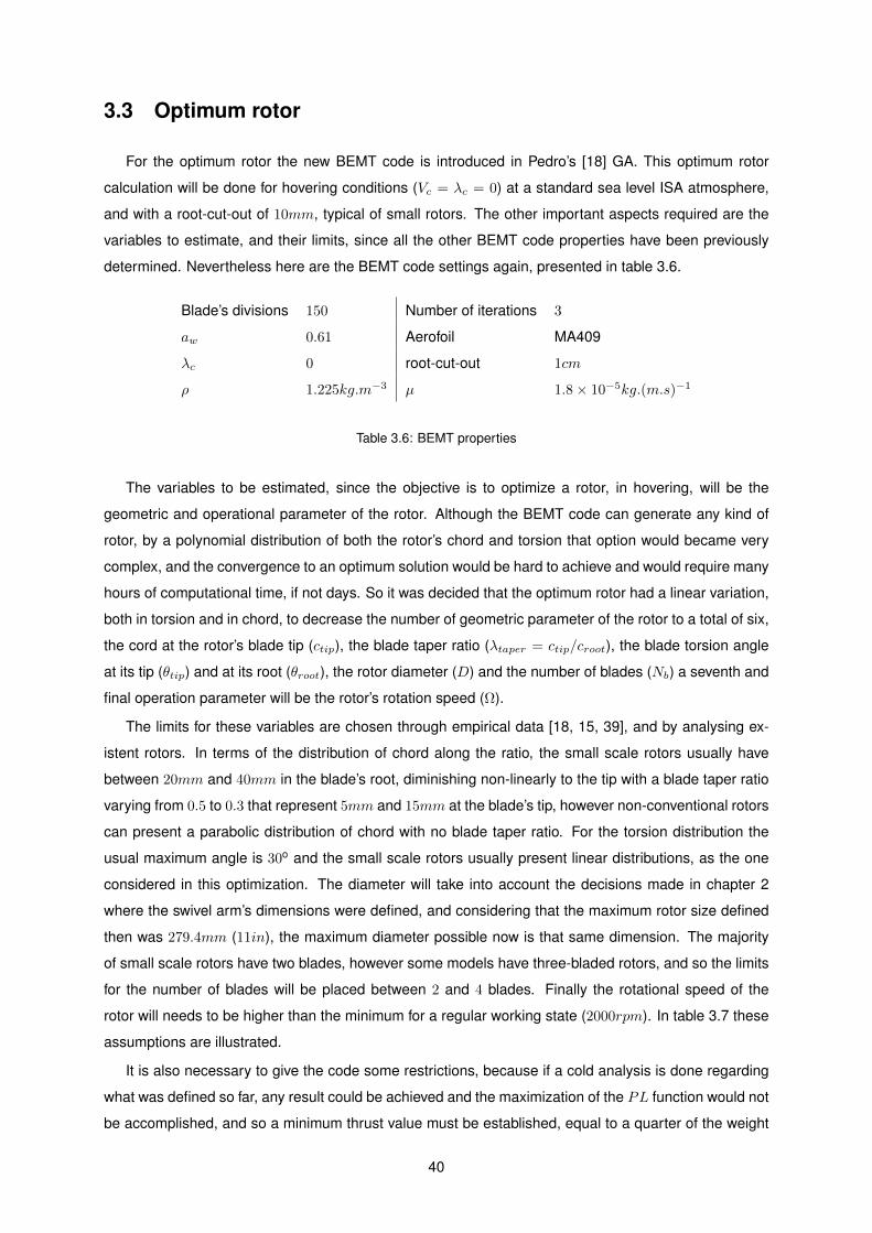
3.3 Optimum rotor

For the optimum rotor the new BEMT code is introduced in Pedro’s [18] GA. This optimum rotor

calculation will be done for hovering conditions (Vc = λc = 0) at a standard sea level ISA atmosphere,

and with a root-cut-out of 10mm, typical of small rotors. The other important aspects required are the

variables to estimate, and their limits, since all the other BEMT code properties have been previously

determined. Nevertheless here are the BEMT code settings again, presented in table 3.6.

Blade’s divisions 150 Number of iterations 3

aw 0.61 Aerofoil MA409

λc 0 root-cut-out 1cm

ρ 1.225kg.m−3 µ 1.8× 10−5kg.(m.s)−1

Table 3.6: BEMT properties

The variables to be estimated, since the objective is to optimize a rotor, in hovering, will be the

geometric and operational parameter of the rotor. Although the BEMT code can generate any kind of

rotor, by a polynomial distribution of both the rotor’s chord and torsion that option would became very

complex, and the convergence to an optimum solution would be hard to achieve and would require many

hours of computational time, if not days. So it was decided that the optimum rotor had a linear variation,

both in torsion and in chord, to decrease the number of geometric parameter of the rotor to a total of six,

the cord at the rotor’s blade tip (ctip), the blade taper ratio (λtaper = ctip/croot), the blade torsion angle

at its tip (θtip) and at its root (θroot), the rotor diameter (D) and the number of blades (Nb) a seventh and

final operation parameter will be the rotor’s rotation speed (Ω).

The limits for these variables are chosen through empirical data [18, 15, 39], and by analysing ex-

istent rotors. In terms of the distribution of chord along the ratio, the small scale rotors usually have

between 20mm and 40mm in the blade’s root, diminishing non-linearly to the tip with a blade taper ratio

varying from 0.5 to 0.3 that represent 5mm and 15mm at the blade’s tip, however non-conventional rotors

can present a parabolic distribution of chord with no blade taper ratio. For the torsion distribution the

usual maximum angle is 30o and the small scale rotors usually present linear distributions, as the one

considered in this optimization. The diameter will take into account the decisions made in chapter 2

where the swivel arm’s dimensions were defined, and considering that the maximum rotor size defined

then was 279.4mm (11in), the maximum diameter possible now is that same dimension. The majority

of small scale rotors have two blades, however some models have three-bladed rotors, and so the limits

for the number of blades will be placed between 2 and 4 blades. Finally the rotational speed of the

rotor will needs to be higher than the minimum for a regular working state (2000rpm). In table 3.7 these

assumptions are illustrated.

It is also necessary to give the code some restrictions, because if a cold analysis is done regarding

what was defined so far, any result could be achieved and the maximization of the PL function would not

be accomplished, and so a minimum thrust value must be established, equal to a quarter of the weight

40

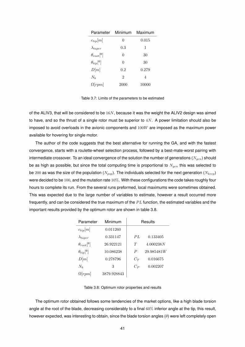
Parameter Minimum Maximum

ctip[m] 0 0.015

λtaper 0.3 1

θroot[o] 0 30

θtip[o] 0 30

D[m] 0.2 0.279

Nb 2 4

Ω[rpm] 2000 10000

Table 3.7: Limits of the parameters to be estimated

of the ALIV3, that will be considered to be 16N , because it was the weight the ALIV2 design was aimed

to have, and so the thrust of a single rotor must be superior to 4N . A power limitation should also be

imposed to avoid overloads in the avionic components and 100W are imposed as the maximum power

available for hovering for single motor.

The author of the code suggests that the best alternative for running the GA, and with the fastest

convergence, starts with a roulette-wheel selection process, followed by a best-mate-worst pairing with

intermediate crossover. To an ideal convergence of the solution the number of generations (Ngen) should

be as high as possible, but since the total computing time is proportional to Ngen this was selected to

be 200 as was the size of the population (Npop). The individuals selected for the next generation (Nkeep)

were decided to be 100, and the mutation rate 10%. With these configurations the code takes roughly four

hours to complete its run. From the several runs preformed, local maximums were sometimes obtained.

This was expected due to the large number of variables to estimate, however a result occurred more

frequently, and can be considered the true maximum of the PL function, the estimated variables and the

important results provided by the optimum rotor are shown in table 3.8.

Parameter Minimum Results

ctip[m] 0.011260

λtaper 0.331147 PL 0.133405

θroot[o] 26.922121 T 4.000238N

θtip[o] 10.086238 P 29.985481W

D[m] 0.278796 CT 0.016675

Nb 3 CP 0.002207

Ω[rpm] 3879.928843

Table 3.8: Optimum rotor properties and results

The optimum rotor obtained follows some tendencies of the market options, like a high blade torsion

angle at the root of the blade, decreasing considerably to a final 60% inferior angle at the tip, this result,

however expected, was interesting to obtain, since the blade torsion angles (θ) were left completely open

41

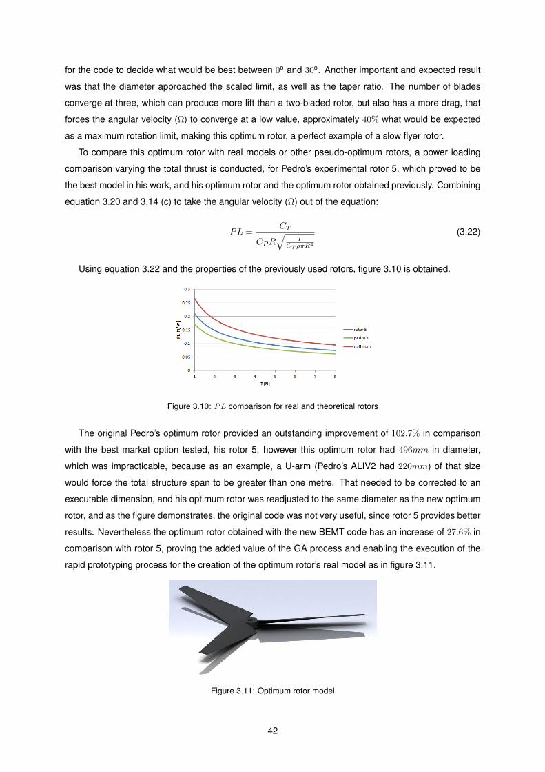
for the code to decide what would be best between 0o and 30o. Another important and expected result

was that the diameter approached the scaled limit, as well as the taper ratio. The number of blades

converge at three, which can produce more lift than a two-bladed rotor, but also has a more drag, that

forces the angular velocity (Ω) to converge at a low value, approximately 40% what would be expected

as a maximum rotation limit, making this optimum rotor, a perfect example of a slow flyer rotor.

To compare this optimum rotor with real models or other pseudo-optimum rotors, a power loading

comparison varying the total thrust is conducted, for Pedro’s experimental rotor 5, which proved to be

the best model in his work, and his optimum rotor and the optimum rotor obtained previously. Combining

equation 3.20 and 3.14 (c) to take the angular velocity (Ω) out of the equation:

PL =CT

CPR√

TCT ρπR4

(3.22)

Using equation 3.22 and the properties of the previously used rotors, figure 3.10 is obtained.

Figure 3.10: PL comparison for real and theoretical rotors

The original Pedro’s optimum rotor provided an outstanding improvement of 102.7% in comparison

with the best market option tested, his rotor 5, however this optimum rotor had 496mm in diameter,

which was impracticable, because as an example, a U-arm (Pedro’s ALIV2 had 220mm) of that size

would force the total structure span to be greater than one metre. That needed to be corrected to an

executable dimension, and his optimum rotor was readjusted to the same diameter as the new optimum

rotor, and as the figure demonstrates, the original code was not very useful, since rotor 5 provides better

results. Nevertheless the optimum rotor obtained with the new BEMT code has an increase of 27.6% in

comparison with rotor 5, proving the added value of the GA process and enabling the execution of the

rapid prototyping process for the creation of the optimum rotor’s real model as in figure 3.11.

Figure 3.11: Optimum rotor model

42

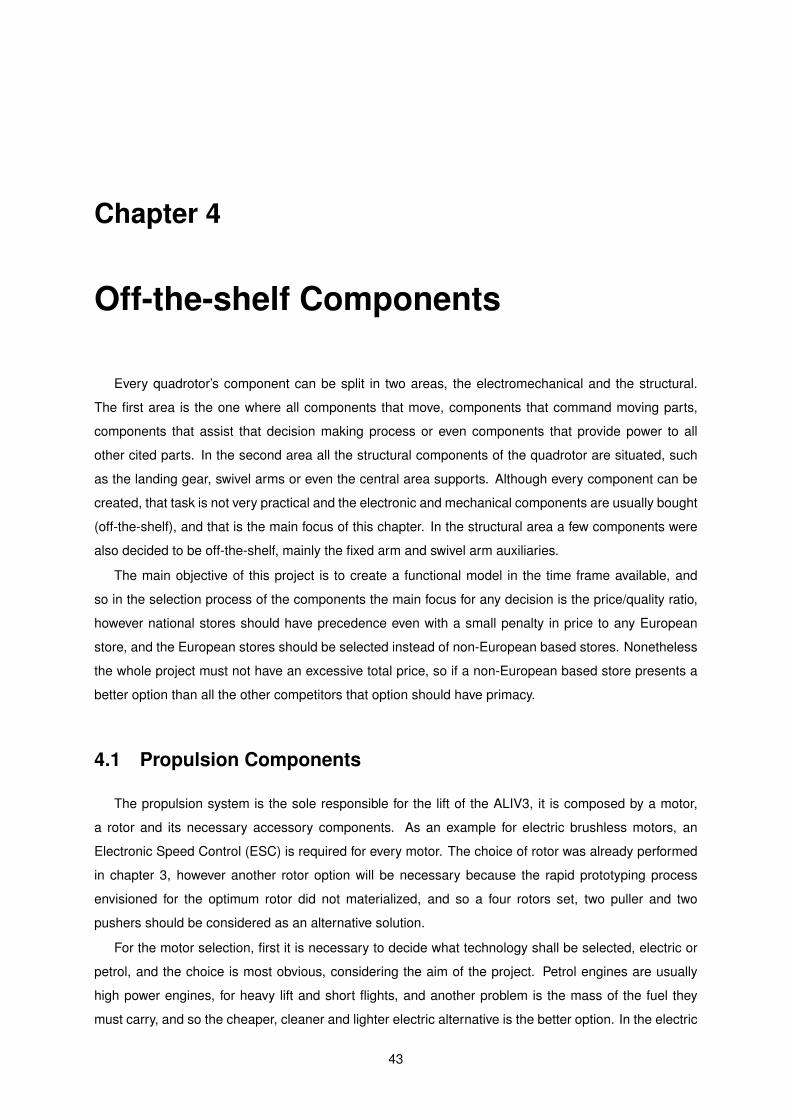
Chapter 4

Off-the-shelf Components

Every quadrotor’s component can be split in two areas, the electromechanical and the structural.

The first area is the one where all components that move, components that command moving parts,

components that assist that decision making process or even components that provide power to all

other cited parts. In the second area all the structural components of the quadrotor are situated, such

as the landing gear, swivel arms or even the central area supports. Although every component can be

created, that task is not very practical and the electronic and mechanical components are usually bought

(off-the-shelf), and that is the main focus of this chapter. In the structural area a few components were

also decided to be off-the-shelf, mainly the fixed arm and swivel arm auxiliaries.

The main objective of this project is to create a functional model in the time frame available, and

so in the selection process of the components the main focus for any decision is the price/quality ratio,

however national stores should have precedence even with a small penalty in price to any European

store, and the European stores should be selected instead of non-European based stores. Nonetheless

the whole project must not have an excessive total price, so if a non-European based store presents a

better option than all the other competitors that option should have primacy.

4.1 Propulsion Components

The propulsion system is the sole responsible for the lift of the ALIV3, it is composed by a motor,

a rotor and its necessary accessory components. As an example for electric brushless motors, an

Electronic Speed Control (ESC) is required for every motor. The choice of rotor was already performed

in chapter 3, however another rotor option will be necessary because the rapid prototyping process

envisioned for the optimum rotor did not materialized, and so a four rotors set, two puller and two

pushers should be considered as an alternative solution.

For the motor selection, first it is necessary to decide what technology shall be selected, electric or

petrol, and the choice is most obvious, considering the aim of the project. Petrol engines are usually

high power engines, for heavy lift and short flights, and another problem is the mass of the fuel they

must carry, and so the cheaper, cleaner and lighter electric alternative is the better option. In the electric

43

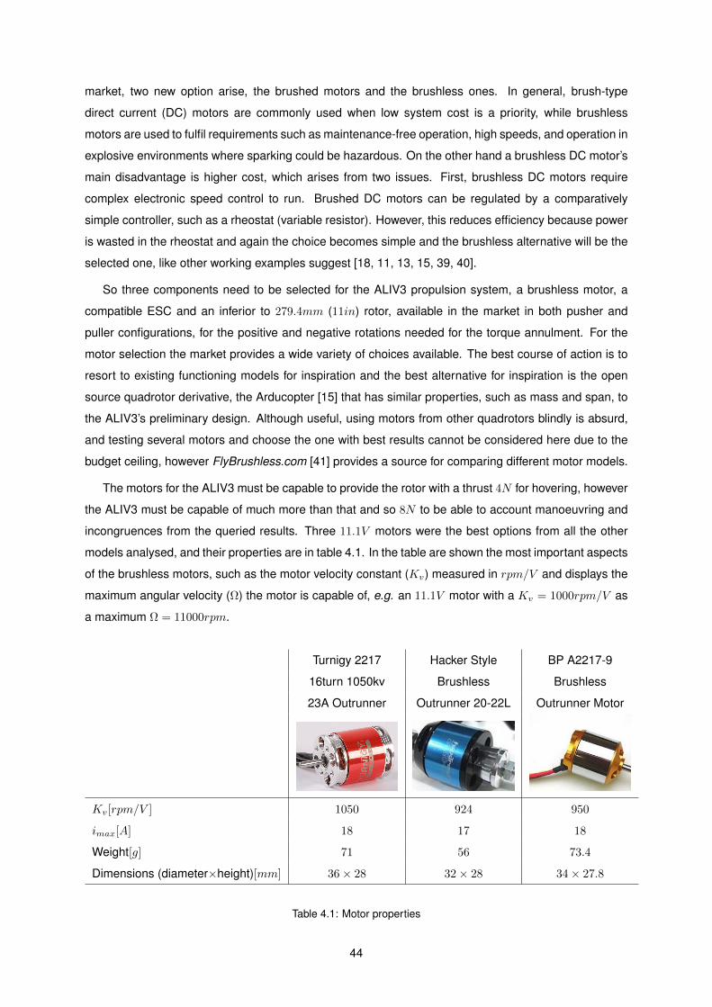
market, two new option arise, the brushed motors and the brushless ones. In general, brush-type

direct current (DC) motors are commonly used when low system cost is a priority, while brushless

motors are used to fulfil requirements such as maintenance-free operation, high speeds, and operation in

explosive environments where sparking could be hazardous. On the other hand a brushless DC motor’s

main disadvantage is higher cost, which arises from two issues. First, brushless DC motors require

complex electronic speed control to run. Brushed DC motors can be regulated by a comparatively

simple controller, such as a rheostat (variable resistor). However, this reduces efficiency because power

is wasted in the rheostat and again the choice becomes simple and the brushless alternative will be the

selected one, like other working examples suggest [18, 11, 13, 15, 39, 40].

So three components need to be selected for the ALIV3 propulsion system, a brushless motor, a

compatible ESC and an inferior to 279.4mm (11in) rotor, available in the market in both pusher and

puller configurations, for the positive and negative rotations needed for the torque annulment. For the

motor selection the market provides a wide variety of choices available. The best course of action is to

resort to existing functioning models for inspiration and the best alternative for inspiration is the open

source quadrotor derivative, the Arducopter [15] that has similar properties, such as mass and span, to

the ALIV3’s preliminary design. Although useful, using motors from other quadrotors blindly is absurd,

and testing several motors and choose the one with best results cannot be considered here due to the

budget ceiling, however FlyBrushless.com [41] provides a source for comparing different motor models.

The motors for the ALIV3 must be capable to provide the rotor with a thrust 4N for hovering, however

the ALIV3 must be capable of much more than that and so 8N to be able to account manoeuvring and

incongruences from the queried results. Three 11.1V motors were the best options from all the other

models analysed, and their properties are in table 4.1. In the table are shown the most important aspects

of the brushless motors, such as the motor velocity constant (Kv) measured in rpm/V and displays the

maximum angular velocity (Ω) the motor is capable of, e.g. an 11.1V motor with a Kv = 1000rpm/V as

a maximum Ω = 11000rpm.

Turnigy 2217 Hacker Style BP A2217-9

16turn 1050kv Brushless Brushless

23A Outrunner Outrunner 20-22L Outrunner Motor

Kv[rpm/V ] 1050 924 950

imax[A] 18 17 18

Weight[g] 71 56 73.4

Dimensions (diameter×height)[mm] 36× 28 32× 28 34× 27.8

Table 4.1: Motor properties

44

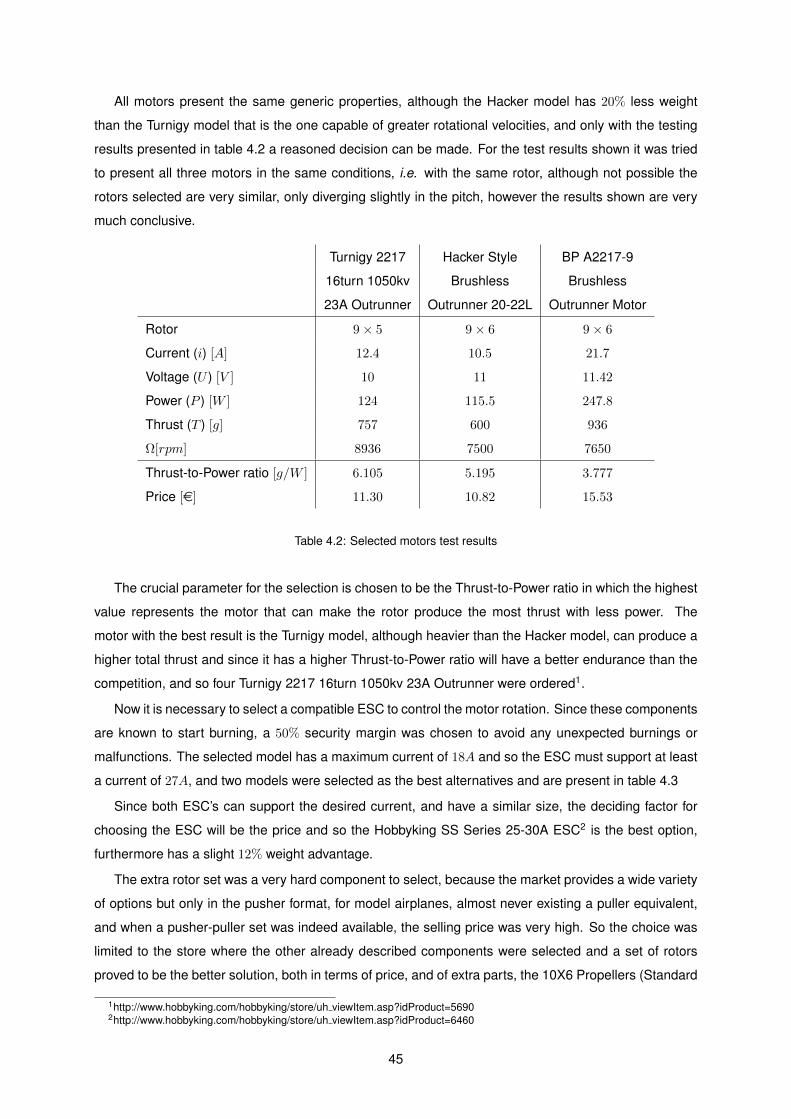
All motors present the same generic properties, although the Hacker model has 20% less weight

than the Turnigy model that is the one capable of greater rotational velocities, and only with the testing

results presented in table 4.2 a reasoned decision can be made. For the test results shown it was tried

to present all three motors in the same conditions, i.e. with the same rotor, although not possible the

rotors selected are very similar, only diverging slightly in the pitch, however the results shown are very

much conclusive.

Turnigy 2217 Hacker Style BP A2217-9

16turn 1050kv Brushless Brushless

23A Outrunner Outrunner 20-22L Outrunner Motor

Rotor 9× 5 9× 6 9× 6

Current (i) [A] 12.4 10.5 21.7

Voltage (U ) [V ] 10 11 11.42

Power (P ) [W ] 124 115.5 247.8

Thrust (T ) [g] 757 600 936

Ω[rpm] 8936 7500 7650

Thrust-to-Power ratio [g/W ] 6.105 5.195 3.777

Price [e] 11.30 10.82 15.53

Table 4.2: Selected motors test results

The crucial parameter for the selection is chosen to be the Thrust-to-Power ratio in which the highest

value represents the motor that can make the rotor produce the most thrust with less power. The

motor with the best result is the Turnigy model, although heavier than the Hacker model, can produce a

higher total thrust and since it has a higher Thrust-to-Power ratio will have a better endurance than the

competition, and so four Turnigy 2217 16turn 1050kv 23A Outrunner were ordered1.

Now it is necessary to select a compatible ESC to control the motor rotation. Since these components

are known to start burning, a 50% security margin was chosen to avoid any unexpected burnings or

malfunctions. The selected model has a maximum current of 18A and so the ESC must support at least

a current of 27A, and two models were selected as the best alternatives and are present in table 4.3

Since both ESC’s can support the desired current, and have a similar size, the deciding factor for

choosing the ESC will be the price and so the Hobbyking SS Series 25-30A ESC2 is the best option,

furthermore has a slight 12% weight advantage.

The extra rotor set was a very hard component to select, because the market provides a wide variety

of options but only in the pusher format, for model airplanes, almost never existing a puller equivalent,

and when a pusher-puller set was indeed available, the selling price was very high. So the choice was

limited to the store where the other already described components were selected and a set of rotors

proved to be the better solution, both in terms of price, and of extra parts, the 10X6 Propellers (Standard

1http://www.hobbyking.com/hobbyking/store/uh viewItem.asp?idProduct=56902http://www.hobbyking.com/hobbyking/store/uh viewItem.asp?idProduct=6460

45

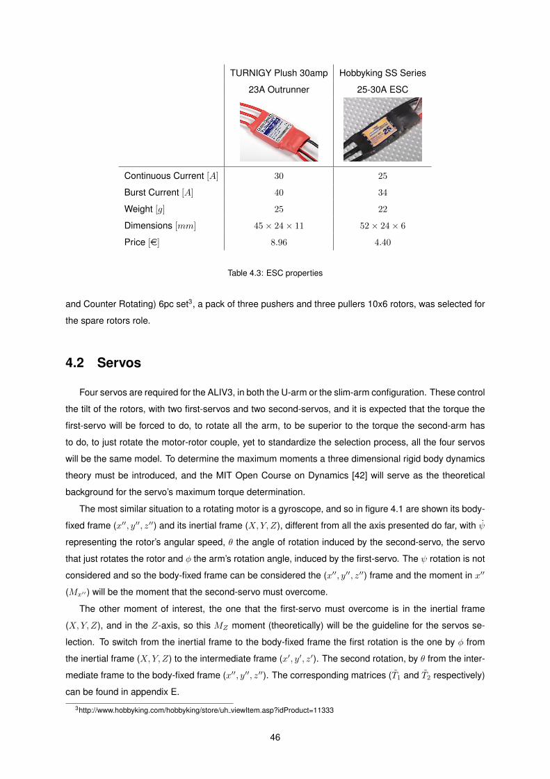
TURNIGY Plush 30amp Hobbyking SS Series

23A Outrunner 25-30A ESC

Continuous Current [A] 30 25

Burst Current [A] 40 34

Weight [g] 25 22

Dimensions [mm] 45× 24× 11 52× 24× 6

Price [e] 8.96 4.40

Table 4.3: ESC properties

and Counter Rotating) 6pc set3, a pack of three pushers and three pullers 10x6 rotors, was selected for

the spare rotors role.

4.2 Servos

Four servos are required for the ALIV3, in both the U-arm or the slim-arm configuration. These control

the tilt of the rotors, with two first-servos and two second-servos, and it is expected that the torque the

first-servo will be forced to do, to rotate all the arm, to be superior to the torque the second-arm has

to do, to just rotate the motor-rotor couple, yet to standardize the selection process, all the four servos

will be the same model. To determine the maximum moments a three dimensional rigid body dynamics

theory must be introduced, and the MIT Open Course on Dynamics [42] will serve as the theoretical

background for the servo’s maximum torque determination.

The most similar situation to a rotating motor is a gyroscope, and so in figure 4.1 are shown its body-

fixed frame (x′′, y′′, z′′) and its inertial frame (X,Y, Z), different from all the axis presented do far, with ψ

representing the rotor’s angular speed, θ the angle of rotation induced by the second-servo, the servo

that just rotates the rotor and φ the arm’s rotation angle, induced by the first-servo. The ψ rotation is not

considered and so the body-fixed frame can be considered the (x′′, y′′, z′′) frame and the moment in x′′

(Mx′′ ) will be the moment that the second-servo must overcome.

The other moment of interest, the one that the first-servo must overcome is in the inertial frame

(X,Y, Z), and in the Z-axis, so this MZ moment (theoretically) will be the guideline for the servos se-

lection. To switch from the inertial frame to the body-fixed frame the first rotation is the one by φ from

the inertial frame (X,Y, Z) to the intermediate frame (x′, y′, z′). The second rotation, by θ from the inter-

mediate frame to the body-fixed frame (x′′, y′′, z′′). The corresponding matrices (T1 and T2 respectively)

can be found in appendix E.

3http://www.hobbyking.com/hobbyking/store/uh viewItem.asp?idProduct=11333

46

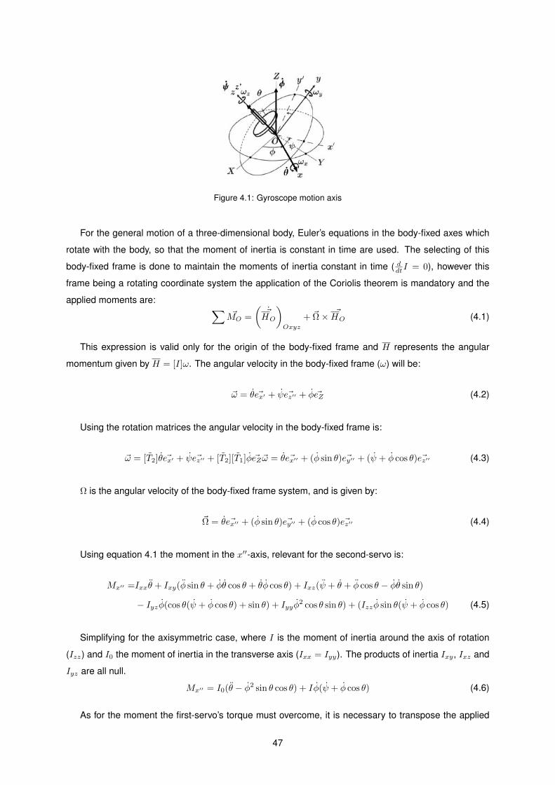
Figure 4.1: Gyroscope motion axis

For the general motion of a three-dimensional body, Euler’s equations in the body-fixed axes which

rotate with the body, so that the moment of inertia is constant in time are used. The selecting of this

body-fixed frame is done to maintain the moments of inertia constant in time ( ddtI = 0), however this

frame being a rotating coordinate system the application of the Coriolis theorem is mandatory and the

applied moments are: ∑~MO =

(~HO

)Oxyz

+ ~Ω× ~HO (4.1)

This expression is valid only for the origin of the body-fixed frame and H represents the angular

momentum given by H = [I]ω. The angular velocity in the body-fixed frame (ω) will be:

~ω = θ ~ex′ + ψ ~ez′′ + φ ~eZ (4.2)

Using the rotation matrices the angular velocity in the body-fixed frame is:

~ω = [T2]θ ~ex′ + ψ ~ez′′ + [T2][T1]φ ~eZ~ω = θ ~ex′′ + (φ sin θ) ~ey′′ + (ψ + φ cos θ) ~ez′′ (4.3)

Ω is the angular velocity of the body-fixed frame system, and is given by:

~Ω = θ ~ex′′ + (φ sin θ) ~ey′′ + (φ cos θ) ~ez′′ (4.4)

Using equation 4.1 the moment in the x′′-axis, relevant for the second-servo is:

Mx′′ =Ixxθ + Ixy(φ sin θ + φθ cos θ + θφ cos θ) + Ixz(ψ + θ + φ cos θ − φθ sin θ)

− Iyzφ(cos θ(ψ + φ cos θ) + sin θ) + Iyyφ2 cos θ sin θ) + (Izzφ sin θ(ψ + φ cos θ) (4.5)

Simplifying for the axisymmetric case, where I is the moment of inertia around the axis of rotation

(Izz) and I0 the moment of inertia in the transverse axis (Ixx = Iyy). The products of inertia Ixy, Ixz and

Iyz are all null.

Mx′′ = I0(θ − φ2 sin θ cos θ) + Iφ(ψ + φ cos θ) (4.6)

As for the moment the first-servo’s torque must overcome, it is necessary to transpose the applied

47

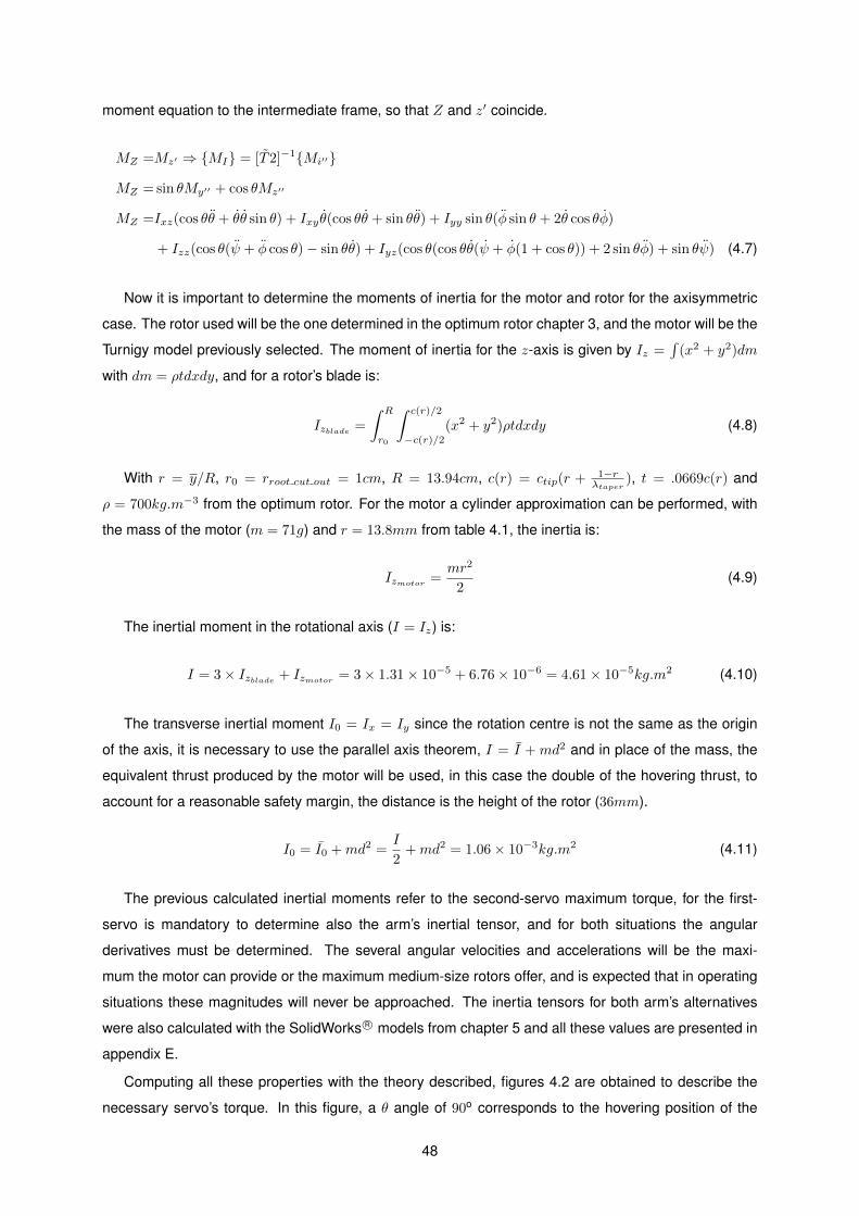
moment equation to the intermediate frame, so that Z and z′ coincide.

MZ =Mz′ ⇒ MI = [T2]−1Mi′′

MZ = sin θMy′′ + cos θMz′′

MZ =Ixz(cos θθ + θθ sin θ) + Ixy θ(cos θθ + sin θθ) + Iyy sin θ(φ sin θ + 2θ cos θφ)

+ Izz(cos θ(ψ + φ cos θ)− sin θθ) + Iyz(cos θ(cos θθ(ψ + φ(1 + cos θ)) + 2 sin θφ) + sin θψ) (4.7)

Now it is important to determine the moments of inertia for the motor and rotor for the axisymmetric

case. The rotor used will be the one determined in the optimum rotor chapter 3, and the motor will be the

Turnigy model previously selected. The moment of inertia for the z-axis is given by Iz =∫

(x2 + y2)dm

with dm = ρtdxdy, and for a rotor’s blade is:

Izblade =

∫ R

r0

∫ c(r)/2

−c(r)/2(x2 + y2)ρtdxdy (4.8)

With r = y/R, r0 = rroot cut out = 1cm, R = 13.94cm, c(r) = ctip(r + 1−rλtaper

), t = .0669c(r) and

ρ = 700kg.m−3 from the optimum rotor. For the motor a cylinder approximation can be performed, with

the mass of the motor (m = 71g) and r = 13.8mm from table 4.1, the inertia is:

Izmotor =mr2

2(4.9)

The inertial moment in the rotational axis (I = Iz) is:

I = 3× Izblade + Izmotor = 3× 1.31× 10−5 + 6.76× 10−6 = 4.61× 10−5kg.m2 (4.10)

The transverse inertial moment I0 = Ix = Iy since the rotation centre is not the same as the origin

of the axis, it is necessary to use the parallel axis theorem, I = I + md2 and in place of the mass, the

equivalent thrust produced by the motor will be used, in this case the double of the hovering thrust, to

account for a reasonable safety margin, the distance is the height of the rotor (36mm).

I0 = I0 +md2 =I

2+md2 = 1.06× 10−3kg.m2 (4.11)

The previous calculated inertial moments refer to the second-servo maximum torque, for the first-

servo is mandatory to determine also the arm’s inertial tensor, and for both situations the angular

derivatives must be determined. The several angular velocities and accelerations will be the maxi-

mum the motor can provide or the maximum medium-size rotors offer, and is expected that in operating

situations these magnitudes will never be approached. The inertia tensors for both arm’s alternatives

were also calculated with the SolidWorks R© models from chapter 5 and all these values are presented in

appendix E.

Computing all these properties with the theory described, figures 4.2 are obtained to describe the

necessary servo’s torque. In this figure, a θ angle of 90o corresponds to the hovering position of the

48

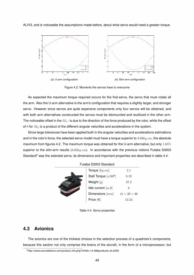
ALIV3, and is noticeable the assumptions made before, about what servo would need a greater torque.

(a) U-arm configuration (b) Slim-arm configuration

Figure 4.2: Moments the servos have to overcome

As expected the maximum torque required occurs for the first-servo, the servo that must rotate all

the arm. Also the U-arm alternative is the arm’s configuration that requires a slightly larger, and stronger

servo. However since servos are quite expensive components only four servos will be obtained, and

with both arm alternatives constructed the servos must be dismounted and reutilized in the other arm.

The noticeable offset in the Mx′′ is due to the direction of the force produced by the rotor, while the offset

of θ for MZ is a product of the different angular velocities and accelerations in the system.

Since large tolerances have been applied both in the angular velocities and accelerations estimations

and in the rotor’s force, the selected servo model must have a torque superior to 3.69kg.cm, the absolute

maximum from figures 4.2. The maximum torque was obtained for the U-arm alternative, but only 1.65%

superior to the slim-arm results (3.63kg.cm). In accordance with the previous notions Futaba S3003

Standard4 was the selected servo, its dimensions and important properties are described in table 4.4.

Futaba S3003 Standard

Torque [kg.cm] 4.1

Stall Torque [s/60o] 0.19

Weight [g] 37.2

Idle current [mA] 8

Dimensions [mm] 41× 20× 36

Price [e] 13.53

Table 4.4: Servo properties

4.3 Avionics

The avionics are one of the trickiest choices in the selection process of a quadrotor’s components,

because this section not only comprise the brains of the aircraft, in the form of a microprocessor, but4http://www.somodelismo.com/product info.php?cPath=14 68&products id=2205

49

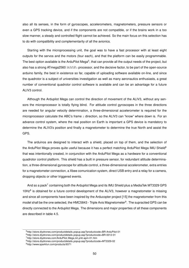
also all its senses, in the form of gyroscopes, accelerometers, magnetometers, pressure sensors or

even a GPS tracking device, and if the components are not compatible, or if the brains work in a too

slow manner, a steady and controlled flight cannot be achieved. So the main focus on this selection has

to do with compatibility and complementarity of all the avionics.

Starting with the microprocessing unit, the goal was to have a fast processor with at least eight

outputs for the servos and the motors (four each), and that the platform can be easily programmable.

The best option available is the ArduPilot Mega5, that can provide all the output needs of the project, but

also has a strong ATmega2560 16MHz processor, and the decisive factor, to be part of the open-source

arduino family, the best in existence so far, capable of uploading software available on-line, and since

the quadrotor is a subject of universities investigation as well as many aeronautics enthusiasts, a great

number of conventional quadrotor control software is available and can be an advantage for a future

ALIV3 control.

Although the Ardupilot Mega can control the direction of movement of the ALIV3, without any sen-

sors the microprocessor is totally flying blind. For attitude control gyroscopes in the three directions

are needed for angular velocity determination, a three-dimensional accelerometer is required for the

microprocessor calculate the ABC’s frame z direction, so the ALIV3 can ”know” where down is. For an

advance control system, where the real position on Earth is important a GPS device is mandatory to

determine the ALIV3’s position and finally a magnetometer to determine the true North and assist the

GPS.

The arduinos are designed to interact with a shield, placed on top of them, and the selection of

the ArduPilot Mega proves quite useful because it has a perfect matching ArduPilot Mega IMU Shield6

that was intentionally created, in conjunction with the ArduPilot Mega as a hardware for a conventional

quadrotor control platform. This shield has a built in pressure sensor, for redundant altitude determina-

tion, a three-dimensional gyroscope for attitude control, a three-dimensional accelerometer, extra entries

for a magnetometer connection, a Xbee comunication system, direct USB entry and a relay for a camera,

dropping objects or other triggered events.

And so a pack7 containing both the Ardupilot Mega and its IMU Shield plus a MediaTek MT3329 GPS

10Hz8 is obtained for a future control development of the ALIV3, however a magnetometer is missing

and since all components have been inspired by the Arducopter project [15] the magnetometer from this

model shall be the one selected, the HMC5843 - Triple Axis Magnetometer9. The supracited GPS can be

directly connected to the Ardupilot Mega. The dimensions and major properties of all these components

are described in table 4.5.

5http://store.diydrones.com/productdetails popup.asp?productcode=BR-ArduPilot-016http://store.diydrones.com/productdetails popup.asp?productcode=BR-0012-017http://store.diydrones.com/ArduPilot Mega kit p/kt-apm-01.htm8http://store.diydrones.com/productdetails popup.asp?productcode=MT3329-029http://www.sparkfun.com/products/9371

50

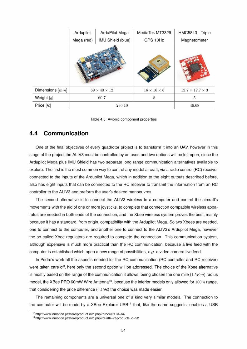
Ardupilot ArduPilot Mega MediaTek MT3329 HMC5843 - Triple

Mega (red) IMU Shield (blue) GPS 10Hz Magnetometer

Dimensions [mm] 69× 40× 12 16× 16× 6 12.7× 12.7× 3

Weight [g] 60.7 8 5

Price [e] 236.10 46.68

Table 4.5: Avionic component properties

4.4 Communication

One of the final objectives of every quadrotor project is to transform it into an UAV, however in this

stage of the project the ALIV3 must be controlled by an user, and two options will be left open, since the

Ardupilot Mega plus IMU Shield has two separate long range communication alternatives available to

explore. The first is the most common way to control any model aircraft, via a radio control (RC) receiver

connected to the inputs of the Ardupilot Mega, which in addition to the eight outputs described before,

also has eight inputs that can be connected to the RC receiver to transmit the information from an RC

controller to the ALIV3 and preform the user’s desired manoeuvres.

The second alternative is to connect the ALIV3 wireless to a computer and control the aircraft’s

movements with the aid of one or more joysticks, to complete that connection compatible wireless appa-

ratus are needed in both ends of the connection, and the Xbee wireless system proves the best, mainly

because it has a standard, from origin, compatibility with the Ardupilot Mega. So two Xbees are needed,

one to connect to the computer, and another one to connect to the ALIV3’s Ardupilot Mega, however

the so called Xbee regulators are required to complete the connection. This communication system,

although expensive is much more practical than the RC communication, because a live feed with the

computer is established which open a new range of possibilities, e.g. a video camera live feed.

In Pedro’s work all the aspects needed for the RC communication (RC controller and RC receiver)

were taken care off, here only the second option will be addressed. The choice of the Xbee alternative

is mostly based on the range of the communication it allows, being chosen the one mile (1.5Km) radius

model, the XBee PRO 60mW Wire Antenna10, because the inferior models only allowed for 100m range,

that considering the price difference (6.15e) the choice was made easier.

The remaining components are a universal one of a kind very similar models. The connection to

the computer will be made by a XBee Explorer USB11 that, like the name suggests, enables a USB

10http://www.inmotion.pt/store/product info.php?products id=6411http://www.inmotion.pt/store/product info.php?cPath=7&products id=52

51

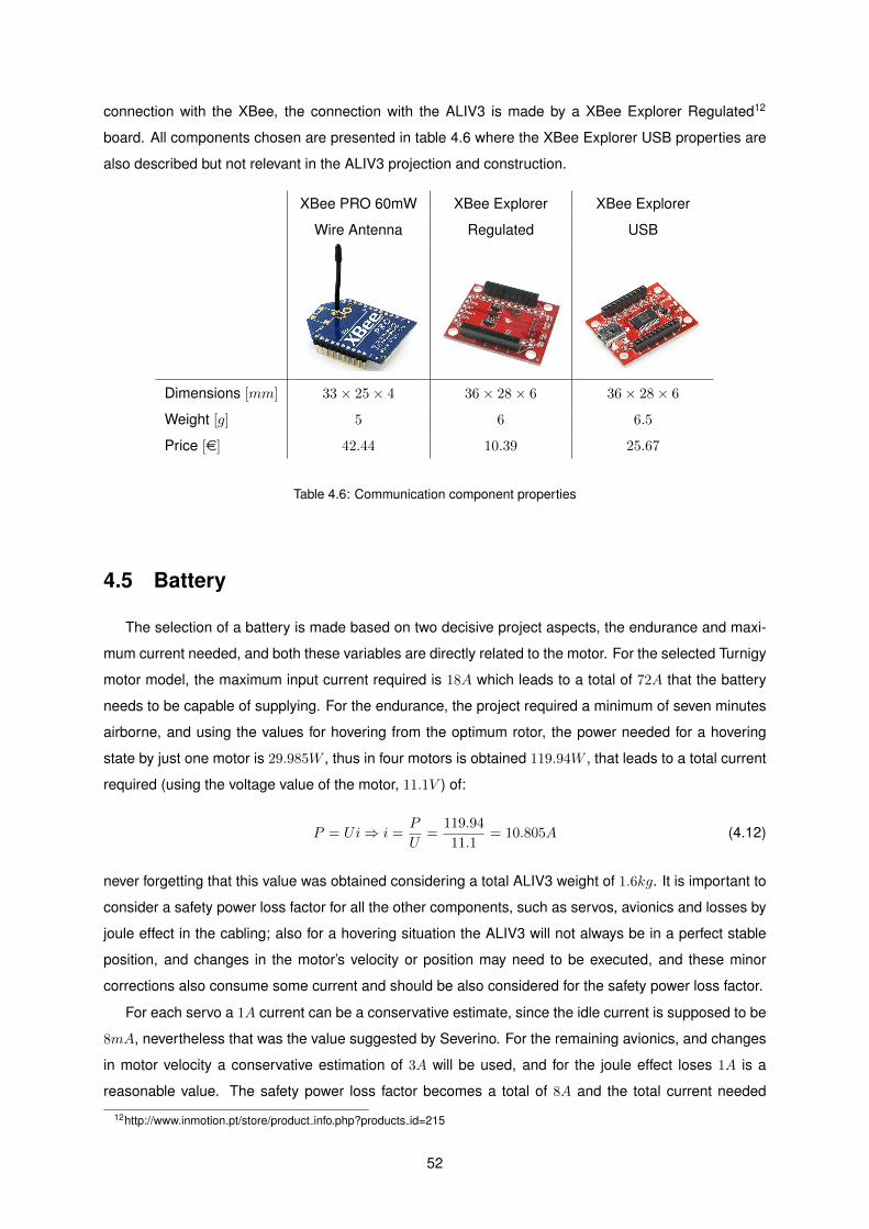
connection with the XBee, the connection with the ALIV3 is made by a XBee Explorer Regulated12

board. All components chosen are presented in table 4.6 where the XBee Explorer USB properties are

also described but not relevant in the ALIV3 projection and construction.

XBee PRO 60mW XBee Explorer XBee Explorer

Wire Antenna Regulated USB

Dimensions [mm] 33× 25× 4 36× 28× 6 36× 28× 6

Weight [g] 5 6 6.5

Price [e] 42.44 10.39 25.67

Table 4.6: Communication component properties

4.5 Battery

The selection of a battery is made based on two decisive project aspects, the endurance and maxi-

mum current needed, and both these variables are directly related to the motor. For the selected Turnigy

motor model, the maximum input current required is 18A which leads to a total of 72A that the battery

needs to be capable of supplying. For the endurance, the project required a minimum of seven minutes

airborne, and using the values for hovering from the optimum rotor, the power needed for a hovering

state by just one motor is 29.985W , thus in four motors is obtained 119.94W , that leads to a total current

required (using the voltage value of the motor, 11.1V ) of:

P = Ui⇒ i =P

U=

119.94

11.1= 10.805A (4.12)

never forgetting that this value was obtained considering a total ALIV3 weight of 1.6kg. It is important to

consider a safety power loss factor for all the other components, such as servos, avionics and losses by

joule effect in the cabling; also for a hovering situation the ALIV3 will not always be in a perfect stable

position, and changes in the motor’s velocity or position may need to be executed, and these minor

corrections also consume some current and should be also considered for the safety power loss factor.

For each servo a 1A current can be a conservative estimate, since the idle current is supposed to be

8mA, nevertheless that was the value suggested by Severino. For the remaining avionics, and changes

in motor velocity a conservative estimation of 3A will be used, and for the joule effect loses 1A is a

reasonable value. The safety power loss factor becomes a total of 8A and the total current needed

12http://www.inmotion.pt/store/product info.php?products id=215

52

comes up to a total of ihover = 18.805A, a slightly higher value however with a good enough margin for

unexpected situations.

The type of battery was chosen to be a lithium polymer (LiPo or Li-poly) battery, the most common

type of battery used nowadays in a wide variety of different technologies, such as PDAs, laptops, model

cars, planes or quadrotors, and even electric urban vehicles. The LiPo batteries are composed of several

identical secondary cells in parallel addition, each cell with a voltage of 3.7V , resulting for the ALIV3

case, to match the motor’s voltage requirements, in the need for a three-cell LiPo battery (11.1V ). The

other two characteristics of the LiPo batteries are the nominal capacity (Cap[mAh]) and the maximum

current discharge rate (C[h−1]) given as a ratio of maximum current over the nominal capacity.

To estimate the minimum nominal capacity needed it is only necessary to use the current for hovering

(18.805A) and the minimum endurance required value.

Capmin = I × Endurance = 18805mA× 10min

60= 3134mAh (4.13)

This way the minimum values for the determination of the required battery are found. The possible

LiPo battery alternatives must be a three-cell 11.1V with maximum current greater than 72A and a

capacity above 3134mAh, furthermore must be as light as possible, so it would not compromise the

1.6kg total weight estimate.

The maximum current discharge rate limit is determined based on both the maximum current and

nominal capacity, and must be above the line of figure 4.3. The usual market LiPo battery alternatives

regarding the value of C are always multiples of 5, and the battery choice must respect the C limit

illustrated or it will not provide the required maximum current.

Figure 4.3: Maximum current discharge rate limit

This study indicates that a 20C battery must have a capacity above 3600mAh and for a 15C battery

the capacity must be greater than 4800mAh. Considering the previous assessment a study of the

batteries weight versus their capacity is made for various maximum current discharge rates (figure 4.4)

and the batteries with the best results are more thoroughly compared in table 4.7.

The maximum current is determined by imax = Cap × C and the endurance is calculated with each

battery capacity and the required current for hovering Endurance = Cap/ihover. All batteries are very

good options and accomplish the desired goals, however one of them, although having a greater penalty

in the total weight of the ALIV3, also has the best result for the endurance, being the one with the largest

capacity, so the decisive factor was actually the price of the component, and the ZIPPY Flightmax

53

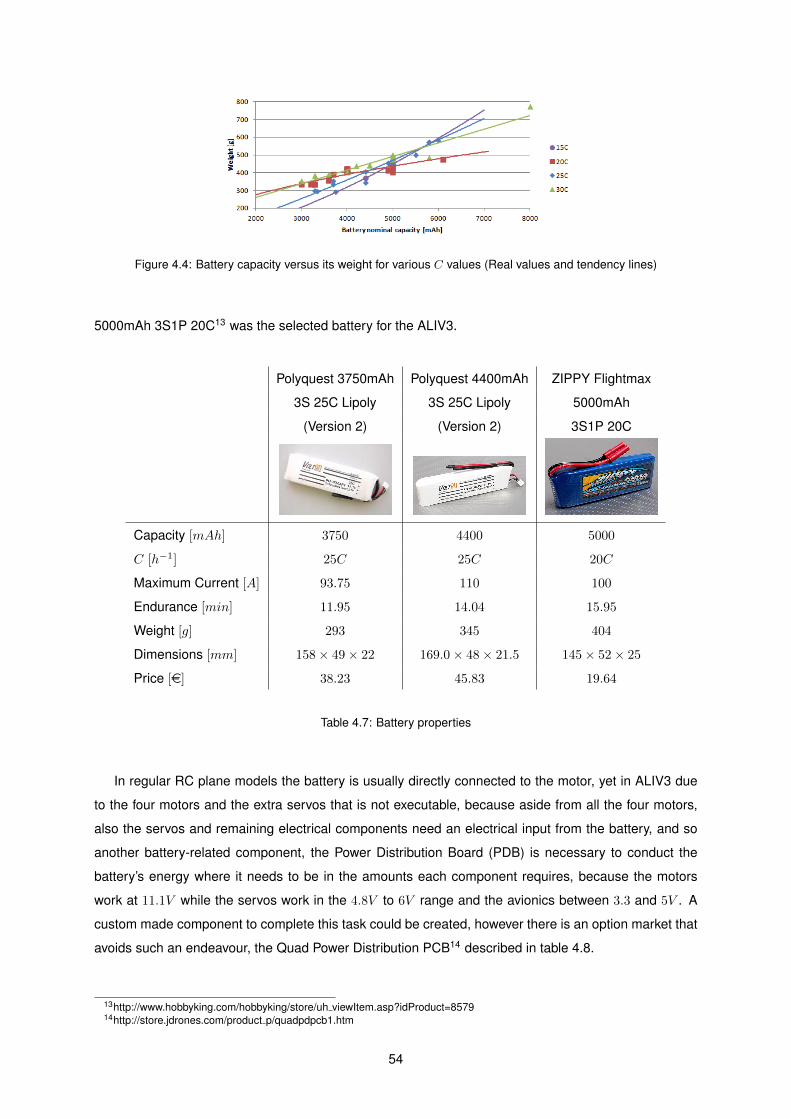
Figure 4.4: Battery capacity versus its weight for various C values (Real values and tendency lines)

5000mAh 3S1P 20C13 was the selected battery for the ALIV3.

Polyquest 3750mAh Polyquest 4400mAh ZIPPY Flightmax

3S 25C Lipoly 3S 25C Lipoly 5000mAh

(Version 2) (Version 2) 3S1P 20C

Capacity [mAh] 3750 4400 5000

C [h−1] 25C 25C 20C

Maximum Current [A] 93.75 110 100

Endurance [min] 11.95 14.04 15.95

Weight [g] 293 345 404

Dimensions [mm] 158× 49× 22 169.0× 48× 21.5 145× 52× 25

Price [e] 38.23 45.83 19.64

Table 4.7: Battery properties

In regular RC plane models the battery is usually directly connected to the motor, yet in ALIV3 due

to the four motors and the extra servos that is not executable, because aside from all the four motors,

also the servos and remaining electrical components need an electrical input from the battery, and so

another battery-related component, the Power Distribution Board (PDB) is necessary to conduct the

battery’s energy where it needs to be in the amounts each component requires, because the motors

work at 11.1V while the servos work in the 4.8V to 6V range and the avionics between 3.3 and 5V . A

custom made component to complete this task could be created, however there is an option market that

avoids such an endeavour, the Quad Power Distribution PCB14 described in table 4.8.

13http://www.hobbyking.com/hobbyking/store/uh viewItem.asp?idProduct=857914http://store.jdrones.com/product p/quadpdpcb1.htm

54

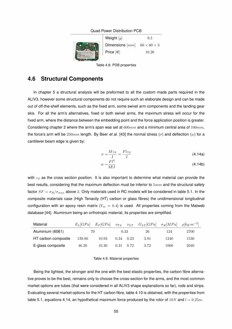
Quad Power Distribution PCB

Weight [g] 9.5

Dimensions [mm] 60× 60× 3

Price [e] 10.26

Table 4.8: PDB properties

4.6 Structural Components

In chapter 5 a structural analysis will be preformed to all the custom made parts required in the

ALIV3, however some structural components do not require such an elaborate design and can be made

out of off-the-shelf elements, such as the fixed arm, some swivel arm components and the landing gear

skis. For all the arm’s alternatives, fixed or both swivel arms, the maximum stress will occur for the

fixed arm, where the distance between the embedding point and the force application position is greater.

Considering chapter 2 where the arm’s span was set at 600mm and a minimum central area of 100mm,

the force’s arm will be 250mm length. By Beer et al. [43] the normal stress (σ) and deflection (w) for a

cantilever beam edge is given by:

σ =MzSI

=FlzSI

(4.14a)

w =Fl3

3EI(4.14b)

with zS as the cross section position. It is also important to determine what material can provide the

best results, considering that the maximum deflection must be inferior to 5mm and the structural safety

factor SF = σR/σmax above 2. Only materials used in RC models will be considered in table 5.1. In the

composite materials case (High Tenacity (HT) carbon or glass fibres) the unidimensional longitudinal

configuration with an epoxy resin matrix (Vm = 0.4) is used. All properties coming from the Matweb

database [44]. Aluminium being an orthotropic material, its properties are simplified.

Material EL[GPa] ET [GPa] νTL νLT GLT [GPa] σR[MPa] ρ[kg.m−3]

Aluminium (6061) 70 0.33 26 124 2700

HT carbon composite 139.80 10.93 0.34 0.23 3.91 1240 1530

E-glass composite 46.20 10.30 0.31 0.72 3.72 1000 2040

Table 4.9: Material properties

Being the lightest, the stronger and the one with the best elastic properties, the carbon fibre alterna-

tive proves to be the best, remains only to choose the cross-section for the arms, and the most common

market options are tubes (that were considered in all ALIV3 shape explanations so far), rods and strips.

Evaluating several market options for the HT carbon fibre, table 4.10 is obtained, with the properties from

table 5.1, equations 4.14, an hypothetical maximum force produced by the rotor of 10N and l = 0.25m.

55

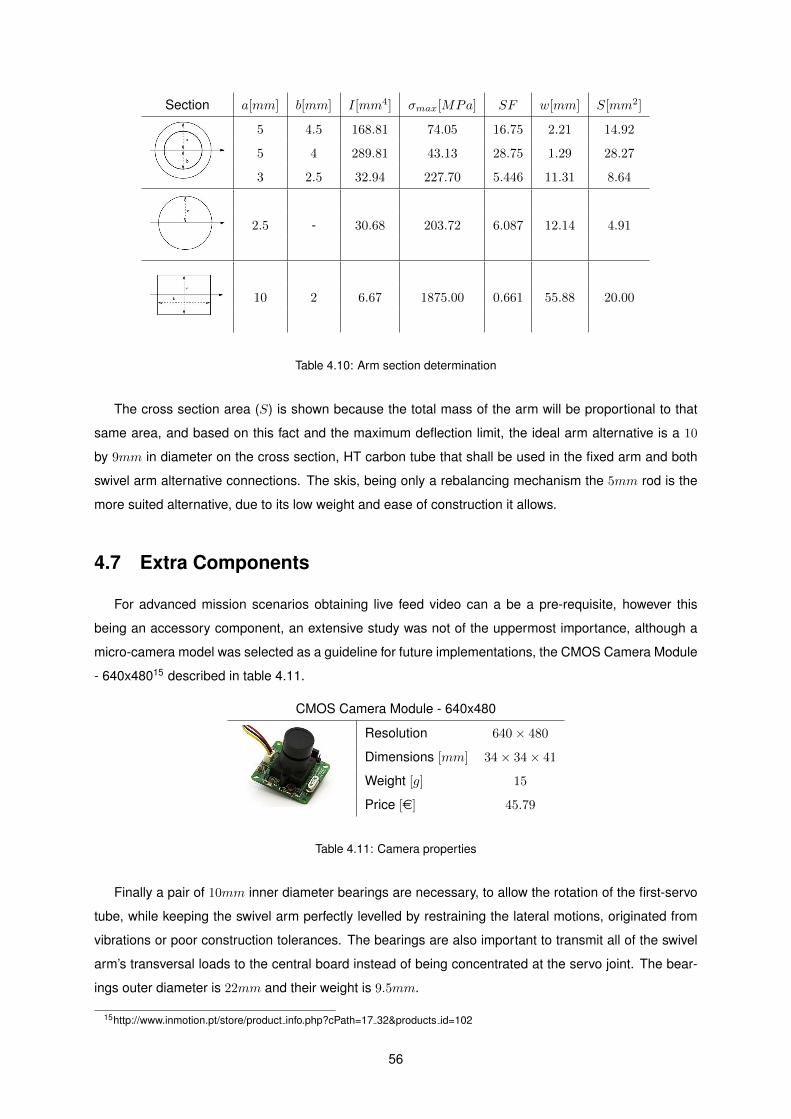
Section a[mm] b[mm] I[mm4] σmax[MPa] SF w[mm] S[mm2]

5 4.5 168.81 74.05 16.75 2.21 14.92

5 4 289.81 43.13 28.75 1.29 28.27

3 2.5 32.94 227.70 5.446 11.31 8.64

2.5 - 30.68 203.72 6.087 12.14 4.91

10 2 6.67 1875.00 0.661 55.88 20.00

Table 4.10: Arm section determination

The cross section area (S) is shown because the total mass of the arm will be proportional to that

same area, and based on this fact and the maximum deflection limit, the ideal arm alternative is a 10

by 9mm in diameter on the cross section, HT carbon tube that shall be used in the fixed arm and both

swivel arm alternative connections. The skis, being only a rebalancing mechanism the 5mm rod is the

more suited alternative, due to its low weight and ease of construction it allows.

4.7 Extra Components

For advanced mission scenarios obtaining live feed video can a be a pre-requisite, however this

being an accessory component, an extensive study was not of the uppermost importance, although a

micro-camera model was selected as a guideline for future implementations, the CMOS Camera Module

- 640x48015 described in table 4.11.

CMOS Camera Module - 640x480

Resolution 640× 480

Dimensions [mm] 34× 34× 41

Weight [g] 15

Price [e] 45.79

Table 4.11: Camera properties

Finally a pair of 10mm inner diameter bearings are necessary, to allow the rotation of the first-servo

tube, while keeping the swivel arm perfectly levelled by restraining the lateral motions, originated from

vibrations or poor construction tolerances. The bearings are also important to transmit all of the swivel

arm’s transversal loads to the central board instead of being concentrated at the servo joint. The bear-

ings outer diameter is 22mm and their weight is 9.5mm.

15http://www.inmotion.pt/store/product info.php?cPath=17 32&products id=102

56

Chapter 5

Design and Construction

The design in any project is an iterative process, where all elements must be combined to achieve a

catalytic effect and a perfectly working system. In this process many alternatives for every components

are made, and by any means the parts created for this project are absolutely adequate for their role, in

theoretical or practical construction terms. Being a first version prototype, the objective was to create a

study platform, with space for improvement, but at the same time that worked according to the predeter-

mined requisites, and this final prototype will be discussed ahead; first it is important to introduce both

the technical and practical theories behind the laminate composites manufacturing.

5.1 Theoretical principles

5.1.1 Laminated composites

Composite materials exist everywhere, even trees are composites, and can be described as any

material composed of at least two elements working together to produce material properties that are

different to the properties of each element per se. In practice, most composites consist of a bulk material,

called the matrix, and a reinforcement, usually in fibre form, added to increase the strength and stiffness

of the matrix. Resin systems such as epoxies and polyesters have limited use for the manufacture

of structures on their own, since their mechanical properties are not very high when compared to, for

example, most metals. However, they have desirable properties, most notably their ability to be easily

formed into complex shapes, and these examples are usually used on laminated composites as matrix.

For the fibre role extremely high tensile and compressive strength materials are used such as glass,

aramid or carbon, yet fibres alone can only exhibit tensile properties along the fibre’s length, and by

combining the two totally different material types, exceptional properties can be obtained. The resin

matrix spreads the load applied to the composite between each of the individual fibres and also protects

the fibres from damage caused by abrasion and impact. The major advantages that composite materials

present are high strengths and stiffnesses, ease of moulding into complex shapes, high environmental

resistance and low densities, making the composites superior to metals for many applications.

Both glass and HT carbon fibre plain woven fabrics are available for this project; however in the

57

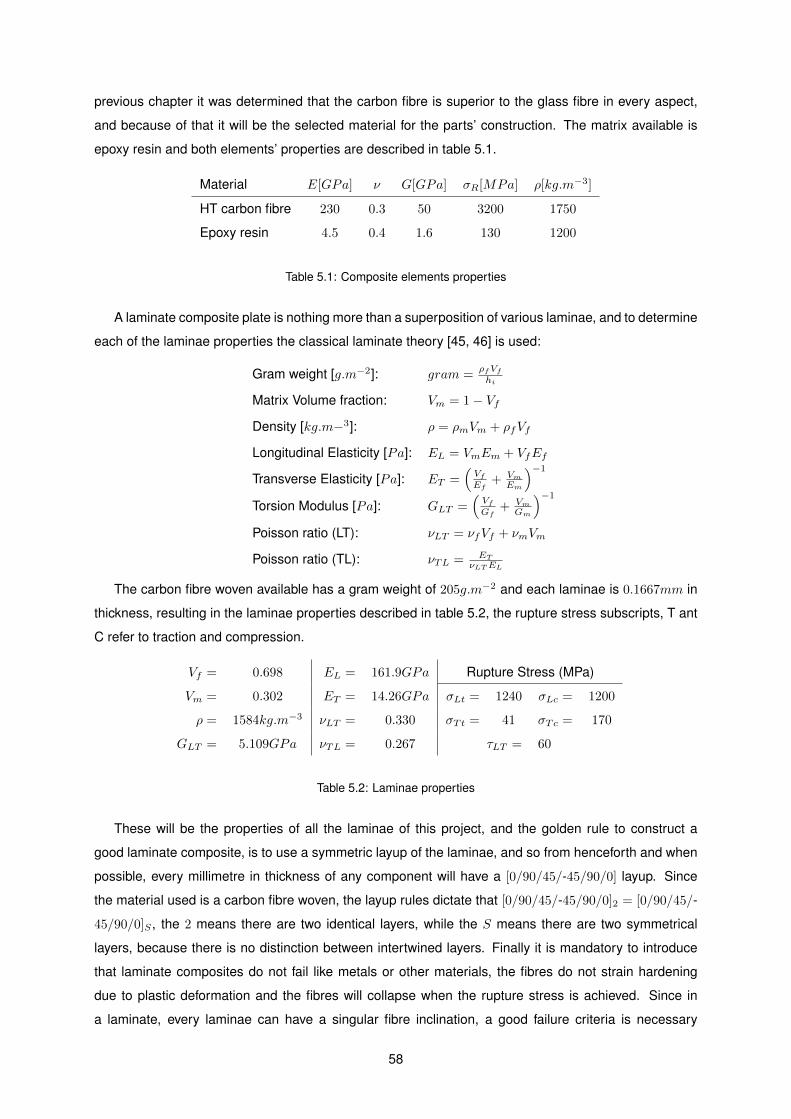
previous chapter it was determined that the carbon fibre is superior to the glass fibre in every aspect,

and because of that it will be the selected material for the parts’ construction. The matrix available is

epoxy resin and both elements’ properties are described in table 5.1.

Material E[GPa] ν G[GPa] σR[MPa] ρ[kg.m−3]

HT carbon fibre 230 0.3 50 3200 1750

Epoxy resin 4.5 0.4 1.6 130 1200

Table 5.1: Composite elements properties

A laminate composite plate is nothing more than a superposition of various laminae, and to determine

each of the laminae properties the classical laminate theory [45, 46] is used:

Gram weight [g.m−2]: gram =ρfVfhi

Matrix Volume fraction: Vm = 1− Vf

Density [kg.m−3]: ρ = ρmVm + ρfVf

Longitudinal Elasticity [Pa]: EL = VmEm + VfEf

Transverse Elasticity [Pa]: ET =(VfEf

+ VmEm

)−1

Torsion Modulus [Pa]: GLT =(VfGf

+ VmGm

)−1

Poisson ratio (LT): νLT = νfVf + νmVm

Poisson ratio (TL): νTL = ETνLTEL

The carbon fibre woven available has a gram weight of 205g.m−2 and each laminae is 0.1667mm in

thickness, resulting in the laminae properties described in table 5.2, the rupture stress subscripts, T ant

C refer to traction and compression.

Vf = 0.698 EL = 161.9GPa Rupture Stress (MPa)

Vm = 0.302 ET = 14.26GPa σLt = 1240 σLc = 1200

ρ = 1584kg.m−3 νLT = 0.330 σTt = 41 σTc = 170

GLT = 5.109GPa νTL = 0.267 τLT = 60

Table 5.2: Laminae properties

These will be the properties of all the laminae of this project, and the golden rule to construct a

good laminate composite, is to use a symmetric layup of the laminae, and so from henceforth and when

possible, every millimetre in thickness of any component will have a [0/90/45/-45/90/0] layup. Since

the material used is a carbon fibre woven, the layup rules dictate that [0/90/45/-45/90/0]2 = [0/90/45/-

45/90/0]S , the 2 means there are two identical layers, while the S means there are two symmetrical

layers, because there is no distinction between intertwined layers. Finally it is mandatory to introduce

that laminate composites do not fail like metals or other materials, the fibres do not strain hardening

due to plastic deformation and the fibres will collapse when the rupture stress is achieved. Since in

a laminate, every laminae can have a singular fibre inclination, a good failure criteria is necessary

58

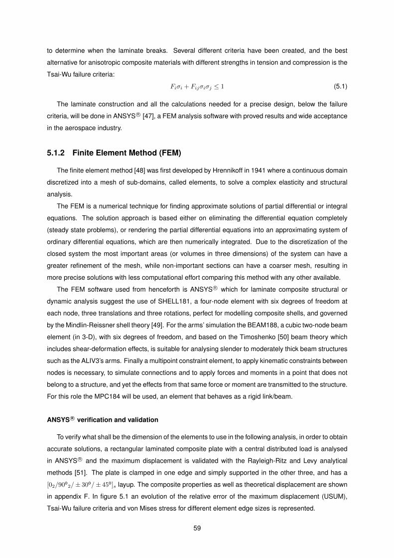
to determine when the laminate breaks. Several different criteria have been created, and the best

alternative for anisotropic composite materials with different strengths in tension and compression is the

Tsai-Wu failure criteria:

Fiσi + Fijσiσj ≤ 1 (5.1)

The laminate construction and all the calculations needed for a precise design, below the failure

criteria, will be done in ANSYS R© [47], a FEM analysis software with proved results and wide acceptance

in the aerospace industry.

5.1.2 Finite Element Method (FEM)

The finite element method [48] was first developed by Hrennikoff in 1941 where a continuous domain

discretized into a mesh of sub-domains, called elements, to solve a complex elasticity and structural

analysis.

The FEM is a numerical technique for finding approximate solutions of partial differential or integral

equations. The solution approach is based either on eliminating the differential equation completely

(steady state problems), or rendering the partial differential equations into an approximating system of

ordinary differential equations, which are then numerically integrated. Due to the discretization of the

closed system the most important areas (or volumes in three dimensions) of the system can have a

greater refinement of the mesh, while non-important sections can have a coarser mesh, resulting in

more precise solutions with less computational effort comparing this method with any other available.

The FEM software used from henceforth is ANSYS R© which for laminate composite structural or

dynamic analysis suggest the use of SHELL181, a four-node element with six degrees of freedom at

each node, three translations and three rotations, perfect for modelling composite shells, and governed

by the Mindlin-Reissner shell theory [49]. For the arms’ simulation the BEAM188, a cubic two-node beam

element (in 3-D), with six degrees of freedom, and based on the Timoshenko [50] beam theory which

includes shear-deformation effects, is suitable for analysing slender to moderately thick beam structures

such as the ALIV3’s arms. Finally a multipoint constraint element, to apply kinematic constraints between

nodes is necessary, to simulate connections and to apply forces and moments in a point that does not

belong to a structure, and yet the effects from that same force or moment are transmitted to the structure.

For this role the MPC184 will be used, an element that behaves as a rigid link/beam.

ANSYS R© verification and validation

To verify what shall be the dimension of the elements to use in the following analysis, in order to obtain

accurate solutions, a rectangular laminated composite plate with a central distributed load is analysed

in ANSYS R© and the maximum displacement is validated with the Rayleigh-Ritz and Levy analytical

methods [51]. The plate is clamped in one edge and simply supported in the other three, and has a

[02/90o2/± 30o/± 45o]s layup. The composite properties as well as theoretical displacement are shown

in appendix F. In figure 5.1 an evolution of the relative error of the maximum displacement (USUM),

Tsai-Wu failure criteria and von Mises stress for different element edge sizes is represented.

59

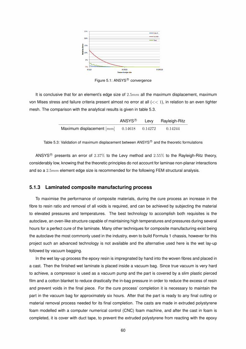
Figure 5.1: ANSYS R© convergence

It is conclusive that for an element’s edge size of 2.5mm all the maximum displacement, maximum

von Mises stress and failure criteria present almost no error at all (<< 1), in relation to an even tighter

mesh. The comparison with the analytical results is given in table 5.3.

ANSYS R© Levy Rayleigh-Ritz

Maximum displacement [mm] 0.14618 0.14272 0.14244

Table 5.3: Validation of maximum displacement between ANSYS R© and the theoretic formulations

ANSYS R© presents an error of 2.37% to the Levy method and 2.55% to the Rayleigh-Ritz theory,

considerably low, knowing that the theoretic principles do not account for laminae non-planar interactions

and so a 2.5mm element edge size is recommended for the following FEM structural analysis.

5.1.3 Laminated composite manufacturing process

To maximise the performance of composite materials, during the cure process an increase in the

fibre to resin ratio and removal of all voids is required, and can be achieved by subjecting the material

to elevated pressures and temperatures. The best technology to accomplish both requisites is the

autoclave, an oven-like structure capable of maintaining high temperatures and pressures during several

hours for a perfect cure of the laminate. Many other techniques for composite manufacturing exist being

the autoclave the most commonly used in the industry, even to build Formula 1 chassis, however for this

project such an advanced technology is not available and the alternative used here is the wet lay-up

followed by vacuum bagging.

In the wet lay-up process the epoxy resin is impregnated by hand into the woven fibres and placed in

a cast. Then the finished wet laminate is placed inside a vacuum bag. Since true vacuum is very hard

to achieve, a compressor is used as a vacuum pump and the part is covered by a slim plastic pierced

film and a cotton blanket to reduce drastically the in-bag pressure in order to reduce the excess of resin

and prevent voids in the final piece. For the cure process’ completion it is necessary to maintain the

part in the vacuum bag for approximately six hours. After that the part is ready to any final cutting or

material removal process needed for its final completion. The casts are made in extruded polystyrene

foam modelled with a computer numerical control (CNC) foam machine, and after the cast in foam is

completed, it is cover with duct tape, to prevent the extruded polystyrene from reacting with the epoxy

60

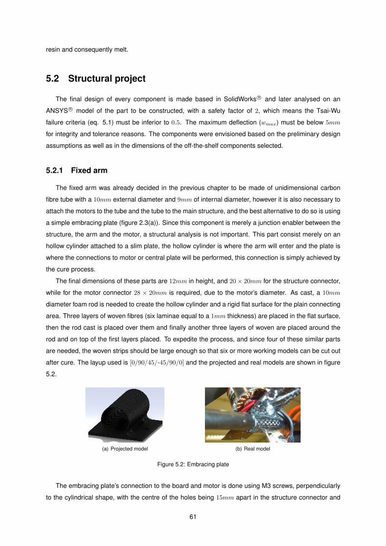
resin and consequently melt.

5.2 Structural project

The final design of every component is made based in SolidWorks R© and later analysed on an

ANSYS R© model of the part to be constructed, with a safety factor of 2, which means the Tsai-Wu

failure criteria (eq. 5.1) must be inferior to 0.5. The maximum deflection (wmax) must be below 5mm

for integrity and tolerance reasons. The components were envisioned based on the preliminary design

assumptions as well as in the dimensions of the off-the-shelf components selected.

5.2.1 Fixed arm

The fixed arm was already decided in the previous chapter to be made of unidimensional carbon

fibre tube with a 10mm external diameter and 9mm of internal diameter, however it is also necessary to

attach the motors to the tube and the tube to the main structure, and the best alternative to do so is using

a simple embracing plate (figure 2.3(a)). Since this component is merely a junction enabler between the

structure, the arm and the motor, a structural analysis is not important. This part consist merely on an

hollow cylinder attached to a slim plate, the hollow cylinder is where the arm will enter and the plate is

where the connections to motor or central plate will be performed, this connection is simply achieved by

the cure process.

The final dimensions of these parts are 12mm in height, and 20× 20mm for the structure connector,

while for the motor connector 28 × 20mm is required, due to the motor’s diameter. As cast, a 10mm

diameter foam rod is needed to create the hollow cylinder and a rigid flat surface for the plain connecting

area. Three layers of woven fibres (six laminae equal to a 1mm thickness) are placed in the flat surface,

then the rod cast is placed over them and finally another three layers of woven are placed around the

rod and on top of the first layers placed. To expedite the process, and since four of these similar parts

are needed, the woven strips should be large enough so that six or more working models can be cut out

after cure. The layup used is [0/90/45/-45/90/0] and the projected and real models are shown in figure

5.2.

(a) Projected model (b) Real model

Figure 5.2: Embracing plate

The embracing plate’s connection to the board and motor is done using M3 screws, perpendicularly

to the cylindrical shape, with the centre of the holes being 15mm apart in the structure connector and

61

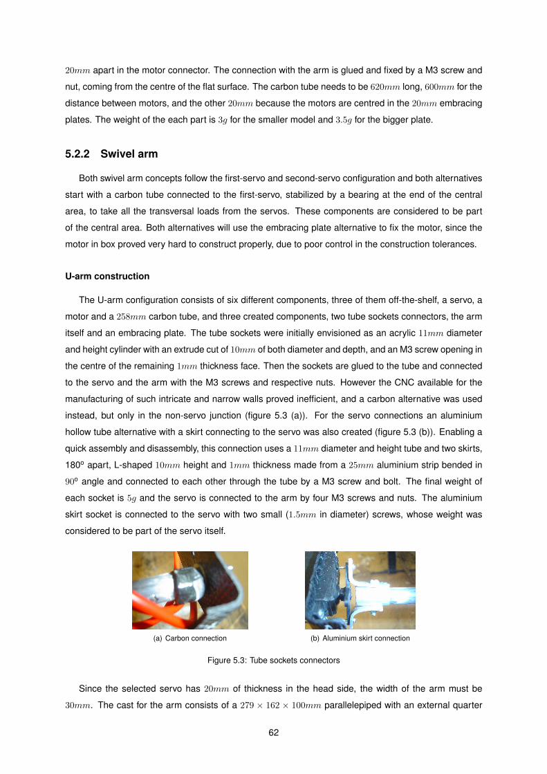
20mm apart in the motor connector. The connection with the arm is glued and fixed by a M3 screw and

nut, coming from the centre of the flat surface. The carbon tube needs to be 620mm long, 600mm for the

distance between motors, and the other 20mm because the motors are centred in the 20mm embracing

plates. The weight of the each part is 3g for the smaller model and 3.5g for the bigger plate.

5.2.2 Swivel arm

Both swivel arm concepts follow the first-servo and second-servo configuration and both alternatives

start with a carbon tube connected to the first-servo, stabilized by a bearing at the end of the central

area, to take all the transversal loads from the servos. These components are considered to be part

of the central area. Both alternatives will use the embracing plate alternative to fix the motor, since the

motor in box proved very hard to construct properly, due to poor control in the construction tolerances.

U-arm construction

The U-arm configuration consists of six different components, three of them off-the-shelf, a servo, a

motor and a 258mm carbon tube, and three created components, two tube sockets connectors, the arm

itself and an embracing plate. The tube sockets were initially envisioned as an acrylic 11mm diameter

and height cylinder with an extrude cut of 10mm of both diameter and depth, and an M3 screw opening in

the centre of the remaining 1mm thickness face. Then the sockets are glued to the tube and connected

to the servo and the arm with the M3 screws and respective nuts. However the CNC available for the

manufacturing of such intricate and narrow walls proved inefficient, and a carbon alternative was used

instead, but only in the non-servo junction (figure 5.3 (a)). For the servo connections an aluminium

hollow tube alternative with a skirt connecting to the servo was also created (figure 5.3 (b)). Enabling a

quick assembly and disassembly, this connection uses a 11mm diameter and height tube and two skirts,

180o apart, L-shaped 10mm height and 1mm thickness made from a 25mm aluminium strip bended in

90o angle and connected to each other through the tube by a M3 screw and bolt. The final weight of

each socket is 5g and the servo is connected to the arm by four M3 screws and nuts. The aluminium

skirt socket is connected to the servo with two small (1.5mm in diameter) screws, whose weight was

considered to be part of the servo itself.

(a) Carbon connection (b) Aluminium skirt connection

Figure 5.3: Tube sockets connectors

Since the selected servo has 20mm of thickness in the head side, the width of the arm must be

30mm. The cast for the arm consists of a 279 × 162 × 100mm parallelepiped with an external quarter

62

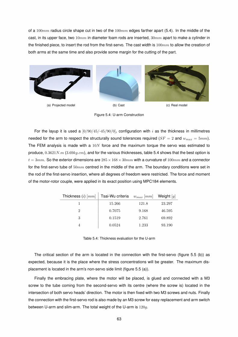
of a 100mm radius circle shape cut in two of the 100mm edges farther apart (5.4). In the middle of the

cast, in its upper face, two 10mm in diameter foam rods are inserted, 30mm apart to make a cylinder in

the finished piece, to insert the rod from the first-servo. The cast width is 100mm to allow the creation of

both arms at the same time and also provide some margin for the cutting of the part.

(a) Projected model (b) Cast (c) Real model

Figure 5.4: U-arm Construction

For the layup it is used a [0/90/45/-45/90/0]i configuration with i as the thickness in millimetres

needed for the arm to respect the structurally sound tolerances required (SF = 2 and wmax = 5mm).

The FEM analysis is made with a 10N force and the maximum torque the servo was estimated to

produce, 0.3621N.m (3.69kg.cm), and for the various thicknesses, table 5.4 shows that the best option is

t = 3mm. So the exterior dimensions are 285× 168× 30mm with a curvature of 100mm and a connector

for the first-servo tube of 50mm centred in the middle of the arm. The boundary conditions were set in

the rod of the first-servo insertion, where all degrees of freedom were restricted. The force and moment

of the motor-rotor couple, were applied in its exact position using MPC184 elements.

Thickness (i) [mm] Tsai-Wu criteria wmax [mm] Weight [g]

1 15.266 121.8 23.297

2 0.7075 9.168 46.595

3 0.1519 2.761 69.892

4 0.0524 1.233 93.190

Table 5.4: Thickness evaluation for the U-arm

The critical section of the arm is located in the connection with the first-servo (figure 5.5 (b)) as

expected, because it is the place where the stress concentrations will be greater. The maximum dis-

placement is located in the arm’s non-servo side limit (figure 5.5 (a)).

Finally the embracing plate, where the motor will be placed, is glued and connected with a M3

screw to the tube coming from the second-servo with its centre (where the screw is) located in the

intersection of both servo heads’ direction. The motor is then fixed with two M3 screws and nuts. Finally

the connection with the first-servo rod is also made by an M3 screw for easy replacement and arm switch

between U-arm and slim-arm. The total weight of the U-arm is 120g.

63

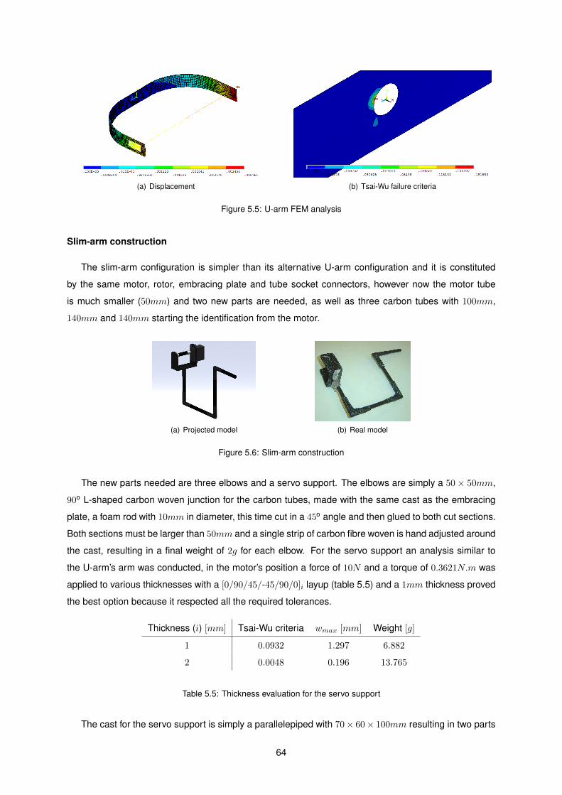
(a) Displacement (b) Tsai-Wu failure criteria

Figure 5.5: U-arm FEM analysis

Slim-arm construction

The slim-arm configuration is simpler than its alternative U-arm configuration and it is constituted

by the same motor, rotor, embracing plate and tube socket connectors, however now the motor tube

is much smaller (50mm) and two new parts are needed, as well as three carbon tubes with 100mm,

140mm and 140mm starting the identification from the motor.

(a) Projected model (b) Real model

Figure 5.6: Slim-arm construction

The new parts needed are three elbows and a servo support. The elbows are simply a 50× 50mm,

90o L-shaped carbon woven junction for the carbon tubes, made with the same cast as the embracing

plate, a foam rod with 10mm in diameter, this time cut in a 45o angle and then glued to both cut sections.

Both sections must be larger than 50mm and a single strip of carbon fibre woven is hand adjusted around

the cast, resulting in a final weight of 2g for each elbow. For the servo support an analysis similar to

the U-arm’s arm was conducted, in the motor’s position a force of 10N and a torque of 0.3621N.m was

applied to various thicknesses with a [0/90/45/-45/90/0]i layup (table 5.5) and a 1mm thickness proved

the best option because it respected all the required tolerances.

Thickness (i) [mm] Tsai-Wu criteria wmax [mm] Weight [g]

1 0.0932 1.297 6.882

2 0.0048 0.196 13.765

Table 5.5: Thickness evaluation for the servo support

The cast for the servo support is simply a parallelepiped with 70× 60× 100mm resulting in two parts

64

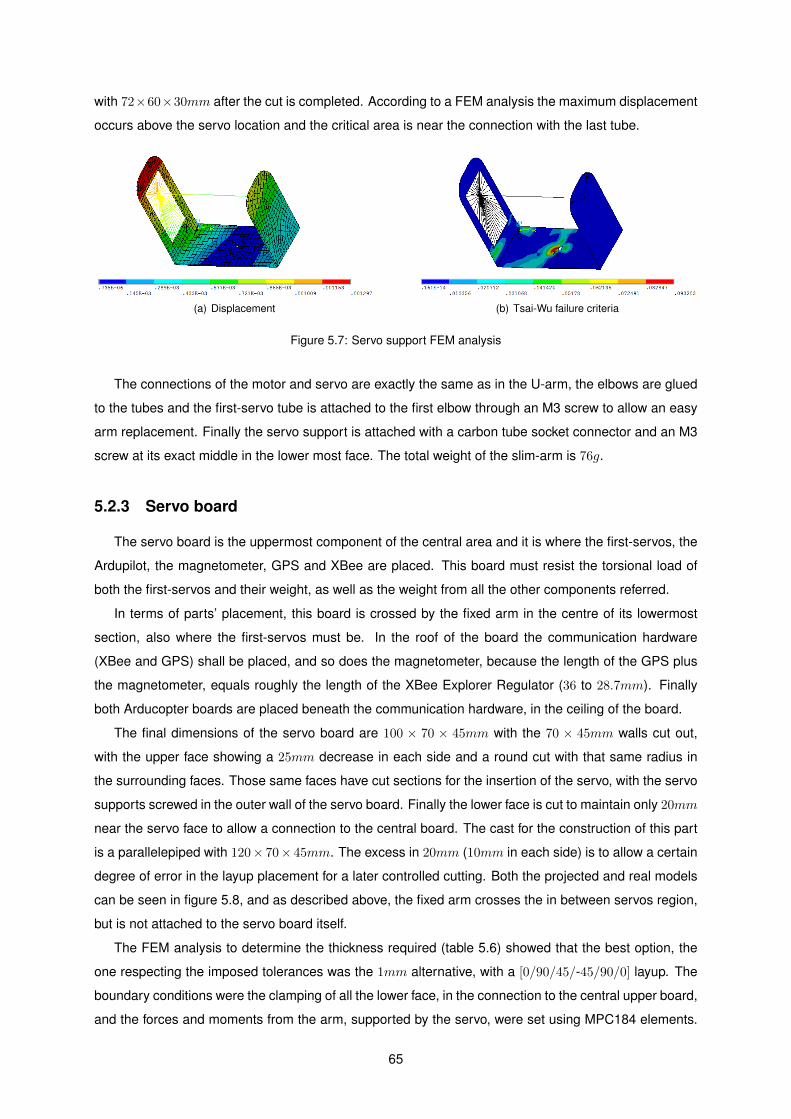
with 72×60×30mm after the cut is completed. According to a FEM analysis the maximum displacement

occurs above the servo location and the critical area is near the connection with the last tube.

(a) Displacement (b) Tsai-Wu failure criteria

Figure 5.7: Servo support FEM analysis

The connections of the motor and servo are exactly the same as in the U-arm, the elbows are glued

to the tubes and the first-servo tube is attached to the first elbow through an M3 screw to allow an easy

arm replacement. Finally the servo support is attached with a carbon tube socket connector and an M3

screw at its exact middle in the lower most face. The total weight of the slim-arm is 76g.

5.2.3 Servo board

The servo board is the uppermost component of the central area and it is where the first-servos, the

Ardupilot, the magnetometer, GPS and XBee are placed. This board must resist the torsional load of

both the first-servos and their weight, as well as the weight from all the other components referred.

In terms of parts’ placement, this board is crossed by the fixed arm in the centre of its lowermost

section, also where the first-servos must be. In the roof of the board the communication hardware

(XBee and GPS) shall be placed, and so does the magnetometer, because the length of the GPS plus

the magnetometer, equals roughly the length of the XBee Explorer Regulator (36 to 28.7mm). Finally

both Arducopter boards are placed beneath the communication hardware, in the ceiling of the board.

The final dimensions of the servo board are 100 × 70 × 45mm with the 70 × 45mm walls cut out,

with the upper face showing a 25mm decrease in each side and a round cut with that same radius in

the surrounding faces. Those same faces have cut sections for the insertion of the servo, with the servo

supports screwed in the outer wall of the servo board. Finally the lower face is cut to maintain only 20mm

near the servo face to allow a connection to the central board. The cast for the construction of this part

is a parallelepiped with 120× 70× 45mm. The excess in 20mm (10mm in each side) is to allow a certain

degree of error in the layup placement for a later controlled cutting. Both the projected and real models

can be seen in figure 5.8, and as described above, the fixed arm crosses the in between servos region,

but is not attached to the servo board itself.

The FEM analysis to determine the thickness required (table 5.6) showed that the best option, the

one respecting the imposed tolerances was the 1mm alternative, with a [0/90/45/-45/90/0] layup. The

boundary conditions were the clamping of all the lower face, in the connection to the central upper board,

and the forces and moments from the arm, supported by the servo, were set using MPC184 elements.

65

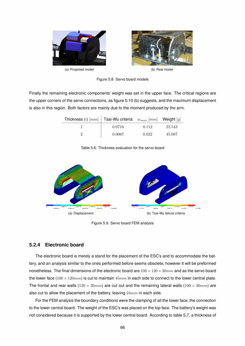
(a) Projected model (b) Real model

Figure 5.8: Servo board models

Finally the remaining electronic components’ weight was set in the upper face. The critical regions are

the upper corners of the servo connections, as figure 5.10 (b) suggests, and the maximum displacement

is also in this region. Both factors are mainly due to the moment produced by the arm.

Thickness (i) [mm] Tsai-Wu criteria wmax [mm] Weight [g]

1 0.0716 0.112 22.543

2 0.0067 0.022 45.087

Table 5.6: Thickness evaluation for the servo board

(a) Displacement (b) Tsai-Wu failure criteria

Figure 5.9: Servo board FEM analysis

5.2.4 Electronic board

The electronic board is merely a stand for the placement of the ESC’s and to accommodate the bat-

tery, and an analysis similar to the ones performed before seems obsolete, however it will be preformed

nonetheless. The final dimensions of the electronic board are 100× 120× 30mm and as the servo board

the lower face (100× 120mm) is cut to maintain 45mm in each side to connect to the lower central plate.

The frontal and rear walls (120 × 30mm) are cut out and the remaining lateral walls (100 × 30mm) are

also cut to allow the placement of the battery, leaving 24mm in each side.

For the FEM analysis the boundary conditions were the clamping of all the lower face, the connection

to the lower central board. The weight of the ESC’s was placed on the top face. The battery’s weight was

not considered because it is supported by the lower central board. According to table 5.7, a thickness of

66

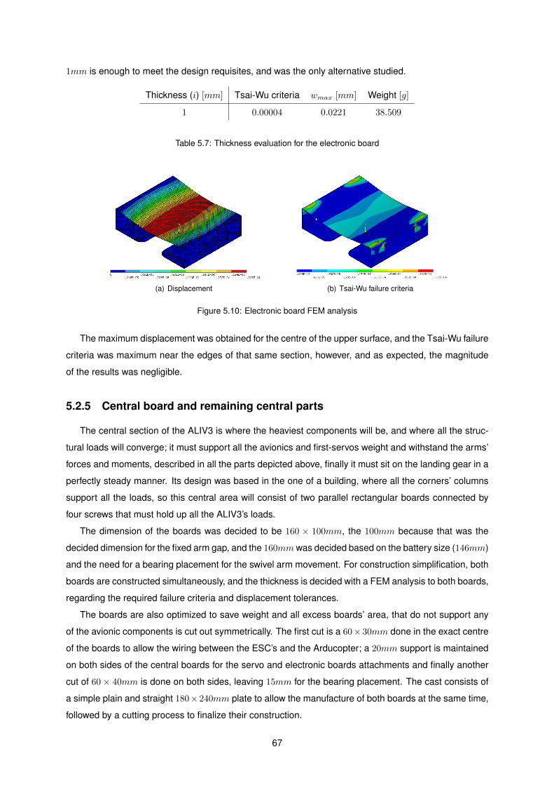
1mm is enough to meet the design requisites, and was the only alternative studied.

Thickness (i) [mm] Tsai-Wu criteria wmax [mm] Weight [g]

1 0.00004 0.0221 38.509

Table 5.7: Thickness evaluation for the electronic board

(a) Displacement (b) Tsai-Wu failure criteria

Figure 5.10: Electronic board FEM analysis

The maximum displacement was obtained for the centre of the upper surface, and the Tsai-Wu failure

criteria was maximum near the edges of that same section, however, and as expected, the magnitude

of the results was negligible.

5.2.5 Central board and remaining central parts

The central section of the ALIV3 is where the heaviest components will be, and where all the struc-

tural loads will converge; it must support all the avionics and first-servos weight and withstand the arms’

forces and moments, described in all the parts depicted above, finally it must sit on the landing gear in a

perfectly steady manner. Its design was based in the one of a building, where all the corners’ columns

support all the loads, so this central area will consist of two parallel rectangular boards connected by

four screws that must hold up all the ALIV3’s loads.

The dimension of the boards was decided to be 160 × 100mm, the 100mm because that was the

decided dimension for the fixed arm gap, and the 160mmwas decided based on the battery size (146mm)

and the need for a bearing placement for the swivel arm movement. For construction simplification, both

boards are constructed simultaneously, and the thickness is decided with a FEM analysis to both boards,

regarding the required failure criteria and displacement tolerances.

The boards are also optimized to save weight and all excess boards’ area, that do not support any

of the avionic components is cut out symmetrically. The first cut is a 60× 30mm done in the exact centre

of the boards to allow the wiring between the ESC’s and the Arducopter; a 20mm support is maintained

on both sides of the central boards for the servo and electronic boards attachments and finally another

cut of 60× 40mm is done on both sides, leaving 15mm for the bearing placement. The cast consists of

a simple plain and straight 180× 240mm plate to allow the manufacture of both boards at the same time,

followed by a cutting process to finalize their construction.

67

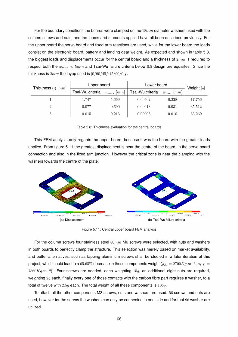
For the boundary conditions the boards were clamped on the 18mm diameter washers used with the

column screws and nuts, and the forces and moments applied have all been described previously. For

the upper board the servo board and fixed arm reactions are used, while for the lower board the loads

consist on the electronic board, battery and landing gear weight. As expected and shown in table 5.8,

the biggest loads and displacements occur for the central board and a thickness of 2mm is required to

respect both the wmax < 5mm and Tsai-Wu failure criteria below 0.5 design prerequisites. Since the

thickness is 2mm the layup used is [0/90/45/-45/90/0]S .

Thickness (i) [mm]Upper board Lower board

Weight [g]Tsai-Wu criteria wmax [mm] Tsai-Wu criteria wmax [mm]

1 1.747 5.669 0.00402 0.228 17.756

2 0.077 0.690 0.00013 0.031 35.512

3 0.015 0.213 0.00003 0.010 53.269

Table 5.8: Thickness evaluation for the central boards

This FEM analysis only regards the upper board, because it was the board with the greater loads

applied. From figure 5.11 the greatest displacement is near the centre of the board, in the servo board

connection and also in the fixed arm junction. However the critical zone is near the clamping with the

washers towards the centre of the plate.

(a) Displacement (b) Tsai-Wu failure criteria

Figure 5.11: Central upper board FEM analysis

For the column screws four stainless steel 80mm M6 screws were selected, with nuts and washers

in both boards to perfectly clamp the structure. This selection was merely based on market availability,

and better alternatives, such as tapping aluminium screws shall be studied in a later iteration of this

project, which could lead to a 65.65% decrease in these components weight (ρAl = 2700Kg.m−3, ρS.S. =

7860Kg.m−3). Four screws are needed, each weighting 15g, an additional eight nuts are required,

weighting 2g each, finally every one of those contacts with the carbon fibre part requires a washer, to a

total of twelve with 2.5g each. The total weight of all these components is 106g.

To attach all the other components M3 screws, nuts and washers are used. 56 screws and nuts are

used, however for the servos the washers can only be connected in one side and for that 96 washer are

utilized.

68

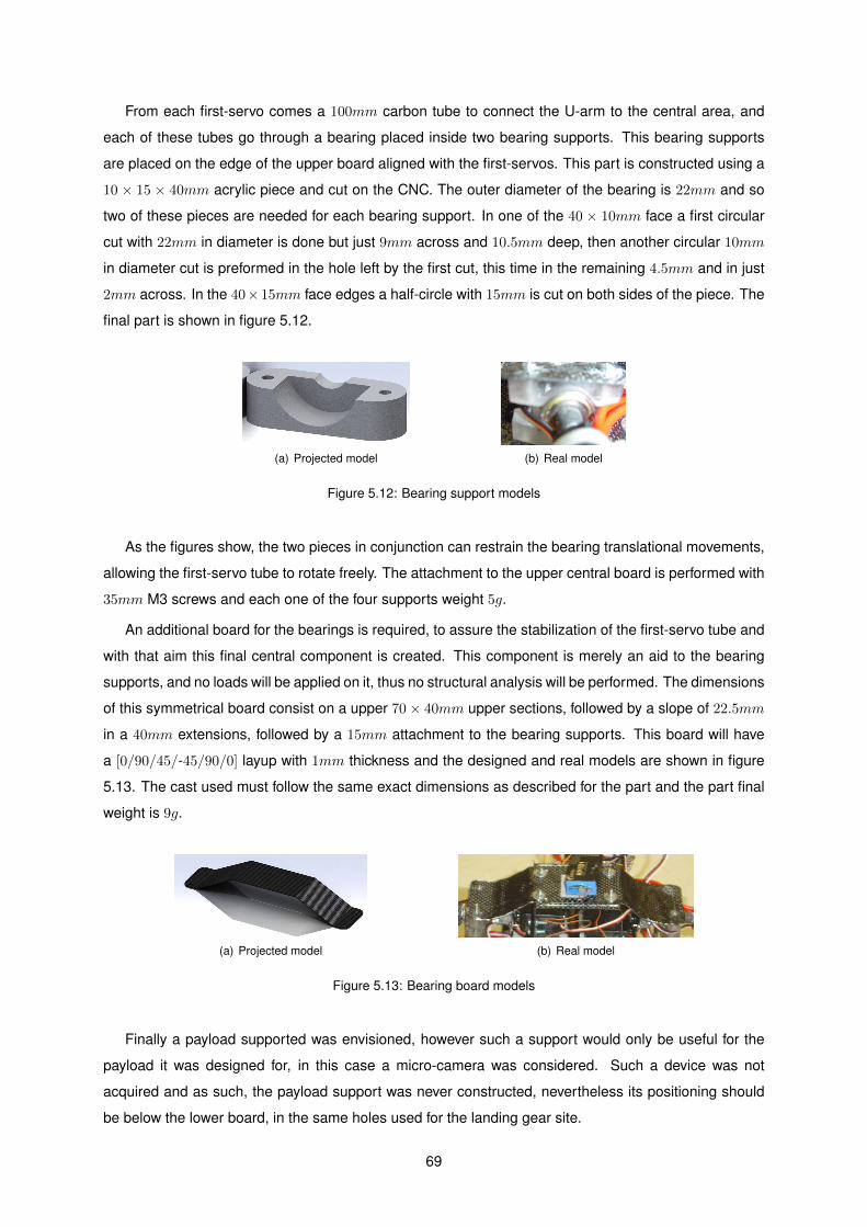
From each first-servo comes a 100mm carbon tube to connect the U-arm to the central area, and

each of these tubes go through a bearing placed inside two bearing supports. This bearing supports

are placed on the edge of the upper board aligned with the first-servos. This part is constructed using a

10 × 15 × 40mm acrylic piece and cut on the CNC. The outer diameter of the bearing is 22mm and so

two of these pieces are needed for each bearing support. In one of the 40 × 10mm face a first circular

cut with 22mm in diameter is done but just 9mm across and 10.5mm deep, then another circular 10mm

in diameter cut is preformed in the hole left by the first cut, this time in the remaining 4.5mm and in just

2mm across. In the 40×15mm face edges a half-circle with 15mm is cut on both sides of the piece. The

final part is shown in figure 5.12.

(a) Projected model (b) Real model

Figure 5.12: Bearing support models

As the figures show, the two pieces in conjunction can restrain the bearing translational movements,

allowing the first-servo tube to rotate freely. The attachment to the upper central board is performed with

35mm M3 screws and each one of the four supports weight 5g.

An additional board for the bearings is required, to assure the stabilization of the first-servo tube and

with that aim this final central component is created. This component is merely an aid to the bearing

supports, and no loads will be applied on it, thus no structural analysis will be performed. The dimensions

of this symmetrical board consist on a upper 70× 40mm upper sections, followed by a slope of 22.5mm

in a 40mm extensions, followed by a 15mm attachment to the bearing supports. This board will have

a [0/90/45/-45/90/0] layup with 1mm thickness and the designed and real models are shown in figure

5.13. The cast used must follow the same exact dimensions as described for the part and the part final

weight is 9g.

(a) Projected model (b) Real model

Figure 5.13: Bearing board models

Finally a payload supported was envisioned, however such a support would only be useful for the

payload it was designed for, in this case a micro-camera was considered. Such a device was not

acquired and as such, the payload support was never constructed, nevertheless its positioning should

be below the lower board, in the same holes used for the landing gear site.

69

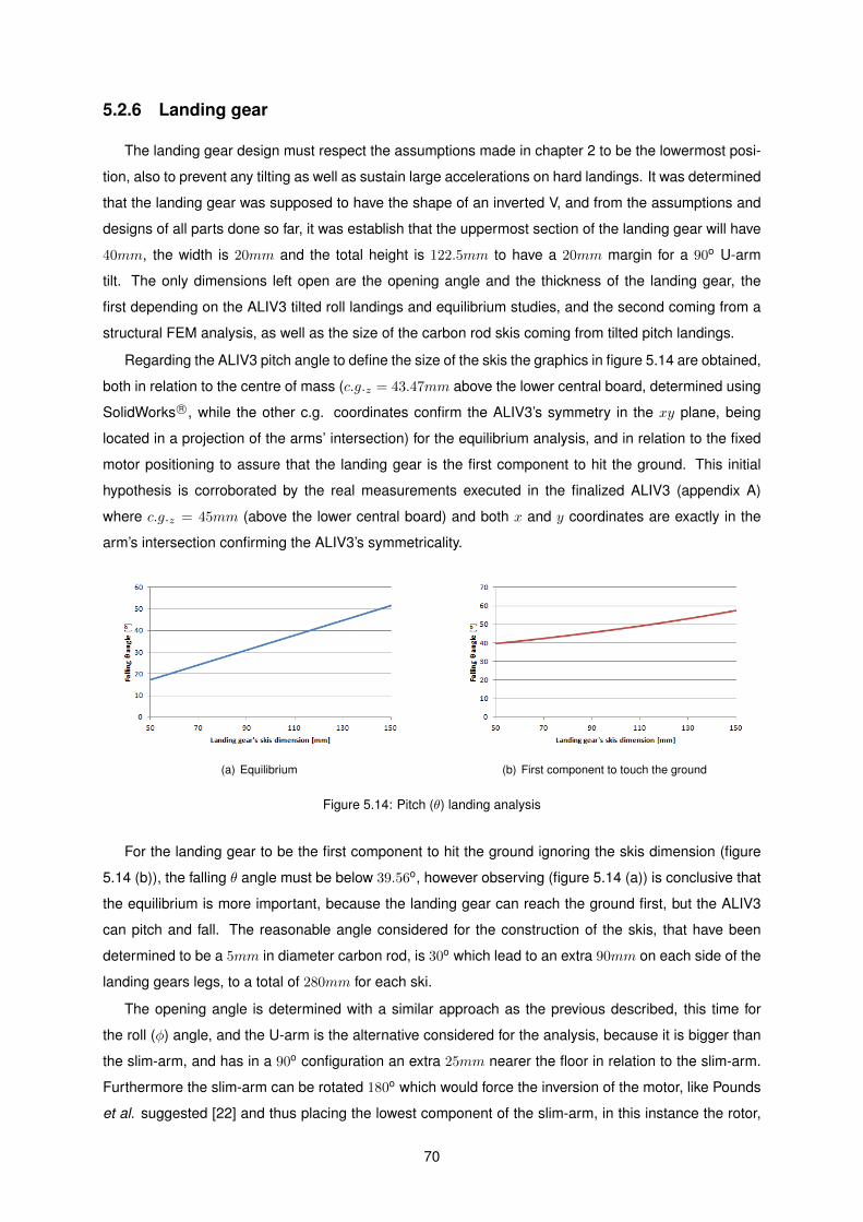
5.2.6 Landing gear

The landing gear design must respect the assumptions made in chapter 2 to be the lowermost posi-

tion, also to prevent any tilting as well as sustain large accelerations on hard landings. It was determined

that the landing gear was supposed to have the shape of an inverted V, and from the assumptions and

designs of all parts done so far, it was establish that the uppermost section of the landing gear will have

40mm, the width is 20mm and the total height is 122.5mm to have a 20mm margin for a 90o U-arm

tilt. The only dimensions left open are the opening angle and the thickness of the landing gear, the

first depending on the ALIV3 tilted roll landings and equilibrium studies, and the second coming from a

structural FEM analysis, as well as the size of the carbon rod skis coming from tilted pitch landings.

Regarding the ALIV3 pitch angle to define the size of the skis the graphics in figure 5.14 are obtained,

both in relation to the centre of mass (c.g.z = 43.47mm above the lower central board, determined using

SolidWorks R©, while the other c.g. coordinates confirm the ALIV3’s symmetry in the xy plane, being

located in a projection of the arms’ intersection) for the equilibrium analysis, and in relation to the fixed

motor positioning to assure that the landing gear is the first component to hit the ground. This initial

hypothesis is corroborated by the real measurements executed in the finalized ALIV3 (appendix A)

where c.g.z = 45mm (above the lower central board) and both x and y coordinates are exactly in the

arm’s intersection confirming the ALIV3’s symmetricality.

(a) Equilibrium (b) First component to touch the ground

Figure 5.14: Pitch (θ) landing analysis

For the landing gear to be the first component to hit the ground ignoring the skis dimension (figure

5.14 (b)), the falling θ angle must be below 39.56o, however observing (figure 5.14 (a)) is conclusive that

the equilibrium is more important, because the landing gear can reach the ground first, but the ALIV3

can pitch and fall. The reasonable angle considered for the construction of the skis, that have been

determined to be a 5mm in diameter carbon rod, is 30o which lead to an extra 90mm on each side of the

landing gears legs, to a total of 280mm for each ski.

The opening angle is determined with a similar approach as the previous described, this time for

the roll (φ) angle, and the U-arm is the alternative considered for the analysis, because it is bigger than

the slim-arm, and has in a 90o configuration an extra 25mm nearer the floor in relation to the slim-arm.

Furthermore the slim-arm can be rotated 180o which would force the inversion of the motor, like Pounds

et al. suggested [22] and thus placing the lowest component of the slim-arm, in this instance the rotor,

70

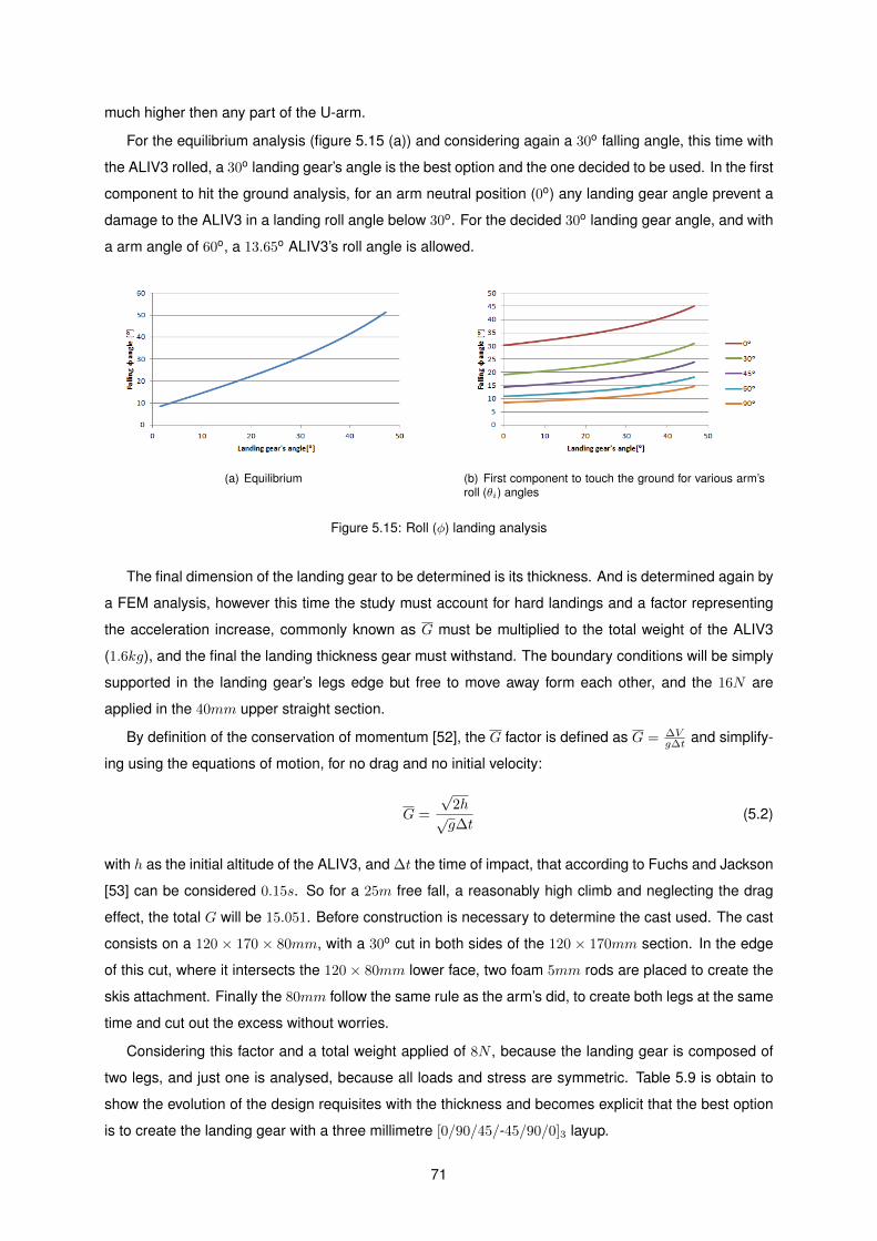
much higher then any part of the U-arm.

For the equilibrium analysis (figure 5.15 (a)) and considering again a 30o falling angle, this time with

the ALIV3 rolled, a 30o landing gear’s angle is the best option and the one decided to be used. In the first

component to hit the ground analysis, for an arm neutral position (0o) any landing gear angle prevent a

damage to the ALIV3 in a landing roll angle below 30o. For the decided 30o landing gear angle, and with

a arm angle of 60o, a 13.65o ALIV3’s roll angle is allowed.

(a) Equilibrium (b) First component to touch the ground for various arm’sroll (θi) angles

Figure 5.15: Roll (φ) landing analysis

The final dimension of the landing gear to be determined is its thickness. And is determined again by

a FEM analysis, however this time the study must account for hard landings and a factor representing

the acceleration increase, commonly known as G must be multiplied to the total weight of the ALIV3

(1.6kg), and the final the landing thickness gear must withstand. The boundary conditions will be simply

supported in the landing gear’s legs edge but free to move away form each other, and the 16N are

applied in the 40mm upper straight section.

By definition of the conservation of momentum [52], the G factor is defined as G = ∆Vg∆t and simplify-

ing using the equations of motion, for no drag and no initial velocity:

G =

√2h

√g∆t

(5.2)

with h as the initial altitude of the ALIV3, and ∆t the time of impact, that according to Fuchs and Jackson

[53] can be considered 0.15s. So for a 25m free fall, a reasonably high climb and neglecting the drag

effect, the total G will be 15.051. Before construction is necessary to determine the cast used. The cast

consists on a 120 × 170 × 80mm, with a 30o cut in both sides of the 120 × 170mm section. In the edge

of this cut, where it intersects the 120× 80mm lower face, two foam 5mm rods are placed to create the

skis attachment. Finally the 80mm follow the same rule as the arm’s did, to create both legs at the same

time and cut out the excess without worries.

Considering this factor and a total weight applied of 8N , because the landing gear is composed of

two legs, and just one is analysed, because all loads and stress are symmetric. Table 5.9 is obtain to

show the evolution of the design requisites with the thickness and becomes explicit that the best option

is to create the landing gear with a three millimetre [0/90/45/-45/90/0]3 layup.

71

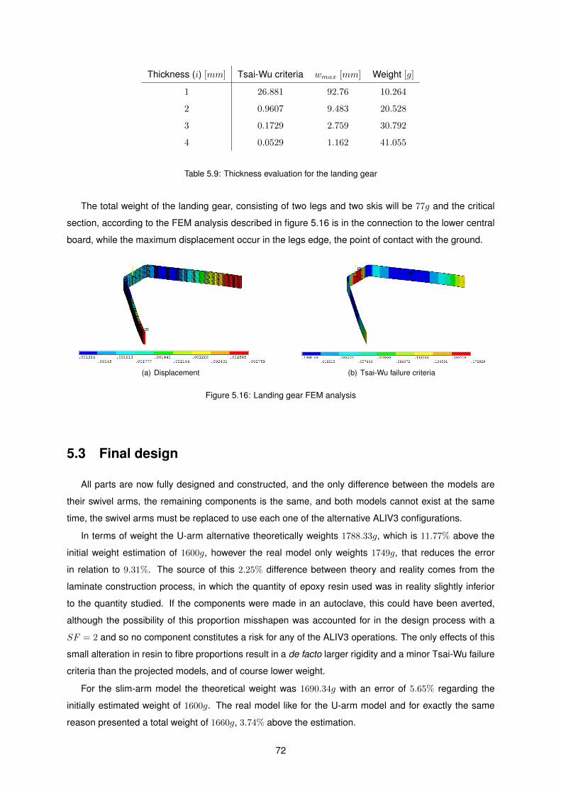
Thickness (i) [mm] Tsai-Wu criteria wmax [mm] Weight [g]

1 26.881 92.76 10.264

2 0.9607 9.483 20.528

3 0.1729 2.759 30.792

4 0.0529 1.162 41.055

Table 5.9: Thickness evaluation for the landing gear

The total weight of the landing gear, consisting of two legs and two skis will be 77g and the critical

section, according to the FEM analysis described in figure 5.16 is in the connection to the lower central

board, while the maximum displacement occur in the legs edge, the point of contact with the ground.

(a) Displacement (b) Tsai-Wu failure criteria

Figure 5.16: Landing gear FEM analysis

5.3 Final design

All parts are now fully designed and constructed, and the only difference between the models are

their swivel arms, the remaining components is the same, and both models cannot exist at the same

time, the swivel arms must be replaced to use each one of the alternative ALIV3 configurations.

In terms of weight the U-arm alternative theoretically weights 1788.33g, which is 11.77% above the

initial weight estimation of 1600g, however the real model only weights 1749g, that reduces the error

in relation to 9.31%. The source of this 2.25% difference between theory and reality comes from the

laminate construction process, in which the quantity of epoxy resin used was in reality slightly inferior

to the quantity studied. If the components were made in an autoclave, this could have been averted,

although the possibility of this proportion misshapen was accounted for in the design process with a

SF = 2 and so no component constitutes a risk for any of the ALIV3 operations. The only effects of this

small alteration in resin to fibre proportions result in a de facto larger rigidity and a minor Tsai-Wu failure

criteria than the projected models, and of course lower weight.

For the slim-arm model the theoretical weight was 1690.34g with an error of 5.65% regarding the

initially estimated weight of 1600g. The real model like for the U-arm model and for exactly the same

reason presented a total weight of 1660g, 3.74% above the estimation.

72

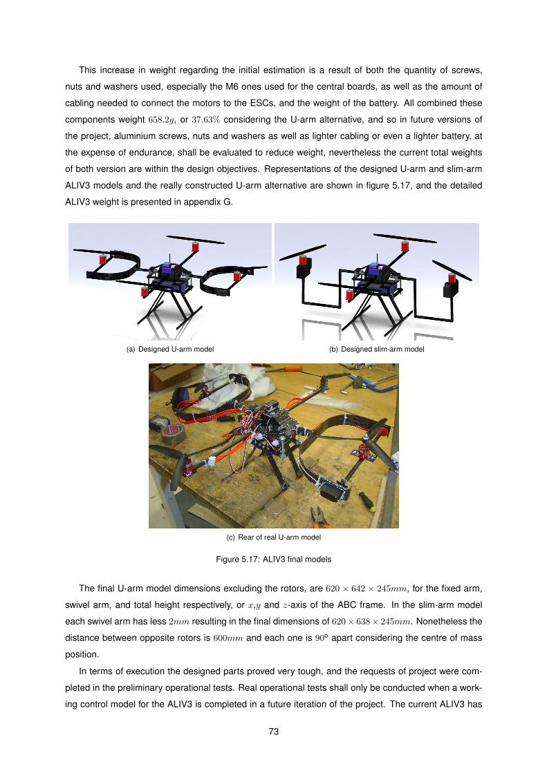
This increase in weight regarding the initial estimation is a result of both the quantity of screws,

nuts and washers used, especially the M6 ones used for the central boards, as well as the amount of

cabling needed to connect the motors to the ESCs, and the weight of the battery. All combined these

components weight 658.2g, or 37.63% considering the U-arm alternative, and so in future versions of

the project, aluminium screws, nuts and washers as well as lighter cabling or even a lighter battery, at

the expense of endurance, shall be evaluated to reduce weight, nevertheless the current total weights

of both version are within the design objectives. Representations of the designed U-arm and slim-arm

ALIV3 models and the really constructed U-arm alternative are shown in figure 5.17, and the detailed

ALIV3 weight is presented in appendix G.

(a) Designed U-arm model (b) Designed slim-arm model

(c) Rear of real U-arm model

Figure 5.17: ALIV3 final models

The final U-arm model dimensions excluding the rotors, are 620 × 642 × 245mm, for the fixed arm,

swivel arm, and total height respectively, or x,y and z-axis of the ABC frame. In the slim-arm model

each swivel arm has less 2mm resulting in the final dimensions of 620× 638× 245mm. Nonetheless the

distance between opposite rotors is 600mm and each one is 90o apart considering the centre of mass

position.

In terms of execution the designed parts proved very tough, and the requests of project were com-

pleted in the preliminary operational tests. Real operational tests shall only be conducted when a work-

ing control model for the ALIV3 is completed in a future iteration of the project. The current ALIV3 has

73

undergone very limited testing, fixed to a table with duct tape, nevertheless in one test, mounted with ro-

tors 5, and inferior motors to the ones selected, with all motors working at theoretically the same power,

less than half the motor capacity, the duct tape peel off the table and the ALIV3 pitched over the table

to a 1.2m fall. Inferior rotors and motor were used because the optimum rotor could not have yet been

really prototyped, and the selected motors are not yet available.

This accident proves three important aspects of the ALIV3 construction and operability. Firstly it has

the power to easily lift itself, with a large margin for the rotor tilting, because if less than half the motor

capacity was being used, with inferior components than the ones selected, means that the ALIV3 can

be lifted with just two motors. Secondly all parts that were designed to withstand only the weight of

the ALIV3, sustained a larger acceleration in collision than the acceleration of a soft regular landing,

furthermore the landing was done in an upside-down position with the servo board hitting the floor,

instead of the landing gear. Using equation 5.2 this fall G’s were equal to 3.30 and so the structure is

even sounder than expected. Thirdly the battery, PDB and ESCs connection is working perfectly. It is

important to note that the tests were performed with an RC connection, because there was no viable

control platform available and no need to use the Ardupilot.

74

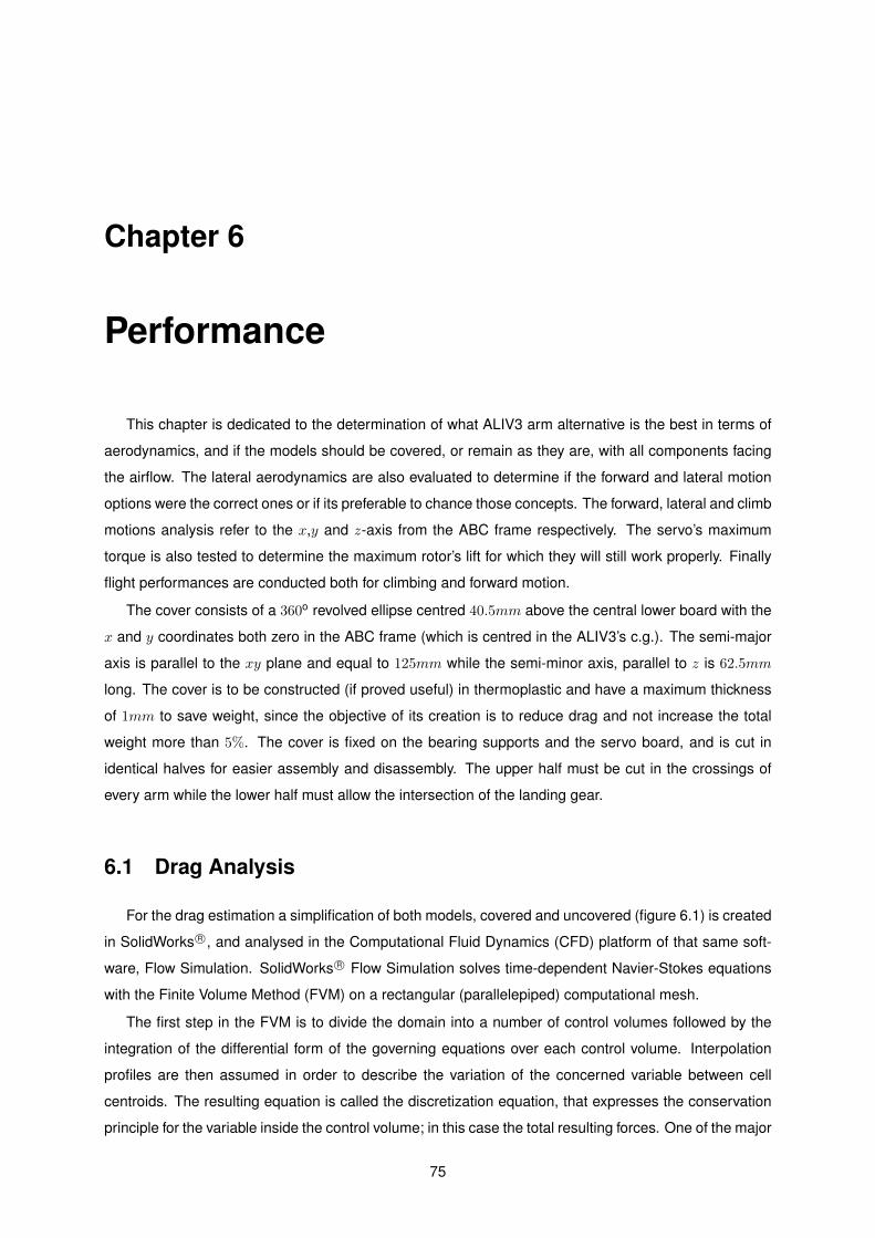
Chapter 6

Performance

This chapter is dedicated to the determination of what ALIV3 arm alternative is the best in terms of

aerodynamics, and if the models should be covered, or remain as they are, with all components facing

the airflow. The lateral aerodynamics are also evaluated to determine if the forward and lateral motion

options were the correct ones or if its preferable to chance those concepts. The forward, lateral and climb

motions analysis refer to the x,y and z-axis from the ABC frame respectively. The servo’s maximum

torque is also tested to determine the maximum rotor’s lift for which they will still work properly. Finally

flight performances are conducted both for climbing and forward motion.

The cover consists of a 360o revolved ellipse centred 40.5mm above the central lower board with the

x and y coordinates both zero in the ABC frame (which is centred in the ALIV3’s c.g.). The semi-major

axis is parallel to the xy plane and equal to 125mm while the semi-minor axis, parallel to z is 62.5mm

long. The cover is to be constructed (if proved useful) in thermoplastic and have a maximum thickness

of 1mm to save weight, since the objective of its creation is to reduce drag and not increase the total

weight more than 5%. The cover is fixed on the bearing supports and the servo board, and is cut in

identical halves for easier assembly and disassembly. The upper half must be cut in the crossings of

every arm while the lower half must allow the intersection of the landing gear.

6.1 Drag Analysis

For the drag estimation a simplification of both models, covered and uncovered (figure 6.1) is created

in SolidWorks R©, and analysed in the Computational Fluid Dynamics (CFD) platform of that same soft-

ware, Flow Simulation. SolidWorks R© Flow Simulation solves time-dependent Navier-Stokes equations

with the Finite Volume Method (FVM) on a rectangular (parallelepiped) computational mesh.

The first step in the FVM is to divide the domain into a number of control volumes followed by the

integration of the differential form of the governing equations over each control volume. Interpolation

profiles are then assumed in order to describe the variation of the concerned variable between cell

centroids. The resulting equation is called the discretization equation, that expresses the conservation

principle for the variable inside the control volume; in this case the total resulting forces. One of the major

75

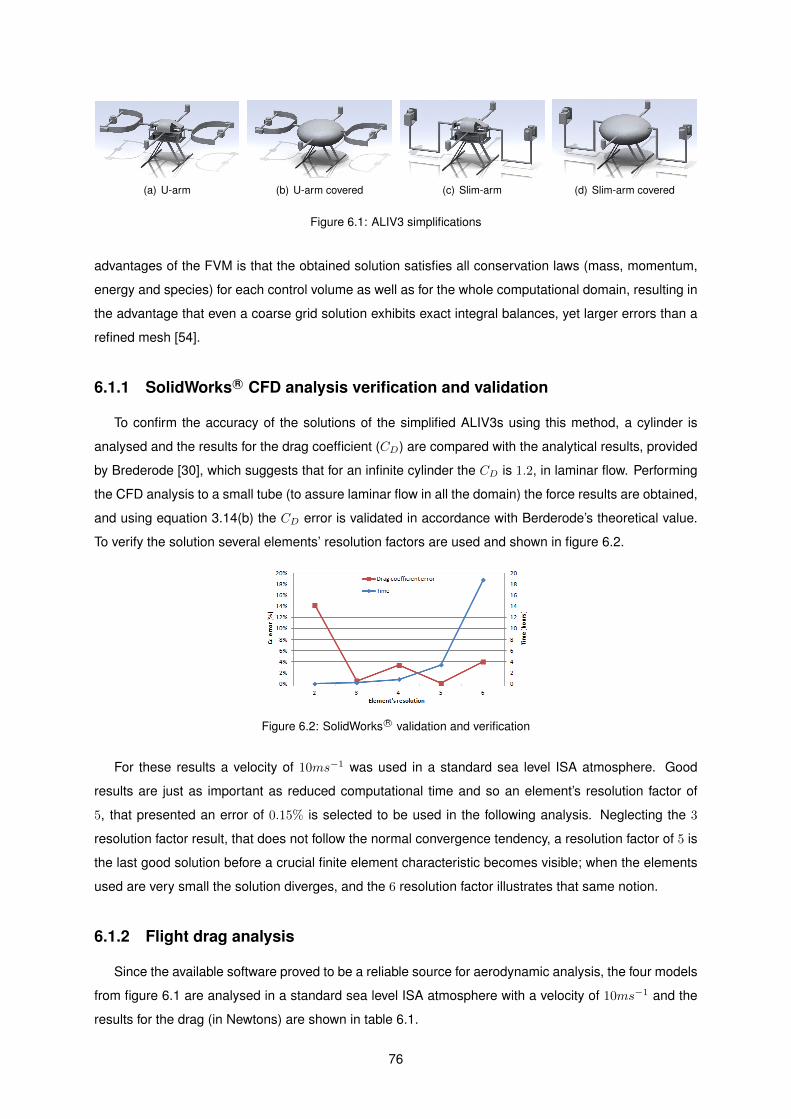
(a) U-arm (b) U-arm covered (c) Slim-arm (d) Slim-arm covered

Figure 6.1: ALIV3 simplifications

advantages of the FVM is that the obtained solution satisfies all conservation laws (mass, momentum,

energy and species) for each control volume as well as for the whole computational domain, resulting in

the advantage that even a coarse grid solution exhibits exact integral balances, yet larger errors than a

refined mesh [54].

6.1.1 SolidWorks R© CFD analysis verification and validation

To confirm the accuracy of the solutions of the simplified ALIV3s using this method, a cylinder is

analysed and the results for the drag coefficient (CD) are compared with the analytical results, provided

by Brederode [30], which suggests that for an infinite cylinder the CD is 1.2, in laminar flow. Performing

the CFD analysis to a small tube (to assure laminar flow in all the domain) the force results are obtained,

and using equation 3.14(b) the CD error is validated in accordance with Berderode’s theoretical value.

To verify the solution several elements’ resolution factors are used and shown in figure 6.2.

Figure 6.2: SolidWorks R© validation and verification

For these results a velocity of 10ms−1 was used in a standard sea level ISA atmosphere. Good

results are just as important as reduced computational time and so an element’s resolution factor of

5, that presented an error of 0.15% is selected to be used in the following analysis. Neglecting the 3

resolution factor result, that does not follow the normal convergence tendency, a resolution factor of 5 is

the last good solution before a crucial finite element characteristic becomes visible; when the elements

used are very small the solution diverges, and the 6 resolution factor illustrates that same notion.

6.1.2 Flight drag analysis

Since the available software proved to be a reliable source for aerodynamic analysis, the four models

from figure 6.1 are analysed in a standard sea level ISA atmosphere with a velocity of 10ms−1 and the

results for the drag (in Newtons) are shown in table 6.1.

76

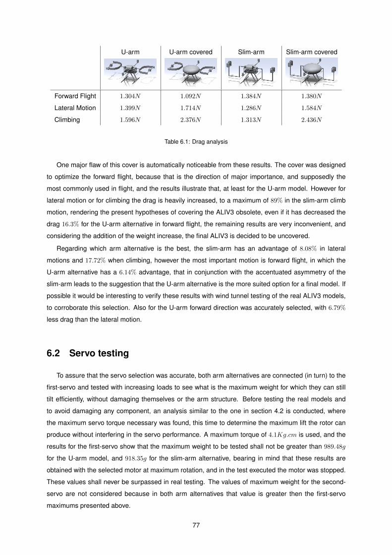
U-arm U-arm covered Slim-arm Slim-arm covered

Forward Flight 1.304N 1.092N 1.384N 1.380N

Lateral Motion 1.399N 1.714N 1.286N 1.584N

Climbing 1.596N 2.376N 1.313N 2.436N

Table 6.1: Drag analysis

One major flaw of this cover is automatically noticeable from these results. The cover was designed

to optimize the forward flight, because that is the direction of major importance, and supposedly the

most commonly used in flight, and the results illustrate that, at least for the U-arm model. However for

lateral motion or for climbing the drag is heavily increased, to a maximum of 89% in the slim-arm climb

motion, rendering the present hypotheses of covering the ALIV3 obsolete, even if it has decreased the

drag 16.3% for the U-arm alternative in forward flight, the remaining results are very inconvenient, and

considering the addition of the weight increase, the final ALIV3 is decided to be uncovered.

Regarding which arm alternative is the best, the slim-arm has an advantage of 8.08% in lateral

motions and 17.72% when climbing, however the most important motion is forward flight, in which the

U-arm alternative has a 6.14% advantage, that in conjunction with the accentuated asymmetry of the

slim-arm leads to the suggestion that the U-arm alternative is the more suited option for a final model. If

possible it would be interesting to verify these results with wind tunnel testing of the real ALIV3 models,

to corroborate this selection. Also for the U-arm forward direction was accurately selected, with 6.79%

less drag than the lateral motion.

6.2 Servo testing

To assure that the servo selection was accurate, both arm alternatives are connected (in turn) to the

first-servo and tested with increasing loads to see what is the maximum weight for which they can still

tilt efficiently, without damaging themselves or the arm structure. Before testing the real models and

to avoid damaging any component, an analysis similar to the one in section 4.2 is conducted, where

the maximum servo torque necessary was found, this time to determine the maximum lift the rotor can

produce without interfering in the servo performance. A maximum torque of 4.1Kg.cm is used, and the

results for the first-servo show that the maximum weight to be tested shall not be greater than 989.48g

for the U-arm model, and 918.35g for the slim-arm alternative, bearing in mind that these results are

obtained with the selected motor at maximum rotation, and in the test executed the motor was stopped.

These values shall never be surpassed in real testing. The values of maximum weight for the second-

servo are not considered because in both arm alternatives that value is greater then the first-servo

maximums presented above.

77

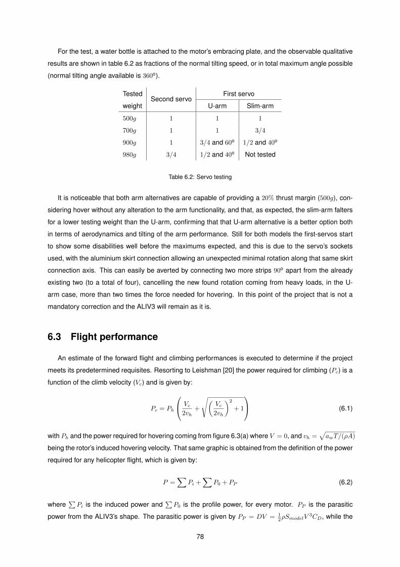
For the test, a water bottle is attached to the motor’s embracing plate, and the observable qualitative

results are shown in table 6.2 as fractions of the normal tilting speed, or in total maximum angle possible

(normal tilting angle available is 360o).

TestedSecond servo

First servo

weight U-arm Slim-arm

500g 1 1 1

700g 1 1 3/4

900g 1 3/4 and 60o 1/2 and 40o

980g 3/4 1/2 and 40o Not tested

Table 6.2: Servo testing

It is noticeable that both arm alternatives are capable of providing a 20% thrust margin (500g), con-

sidering hover without any alteration to the arm functionality, and that, as expected, the slim-arm falters

for a lower testing weight than the U-arm, confirming that that U-arm alternative is a better option both

in terms of aerodynamics and tilting of the arm performance. Still for both models the first-servos start

to show some disabilities well before the maximums expected, and this is due to the servo’s sockets

used, with the aluminium skirt connection allowing an unexpected minimal rotation along that same skirt

connection axis. This can easily be averted by connecting two more strips 90o apart from the already

existing two (to a total of four), cancelling the new found rotation coming from heavy loads, in the U-

arm case, more than two times the force needed for hovering. In this point of the project that is not a

mandatory correction and the ALIV3 will remain as it is.

6.3 Flight performance

An estimate of the forward flight and climbing performances is executed to determine if the project

meets its predetermined requisites. Resorting to Leishman [20] the power required for climbing (Pc) is a

function of the climb velocity (Vc) and is given by:

Pc = Ph

Vc2vh

+

√(Vc2vh

)2

+ 1

(6.1)

with Ph and the power required for hovering coming from figure 6.3(a) where V = 0, and vh =√awT/(ρA)

being the rotor’s induced hovering velocity. That same graphic is obtained from the definition of the power

required for any helicopter flight, which is given by:

P =∑

Pi +∑

P0 + PP (6.2)

where∑Pi is the induced power and

∑P0 is the profile power, for every motor. PP is the parasitic

power from the ALIV3’s shape. The parasitic power is given by PP = DV = 12ρSmodelV

3CD, while the

78

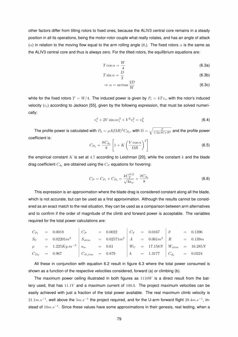
other factors differ from tilting rotors to fixed ones, because the ALIV3 central core remains in a steady

position in all its operations, being the motor-rotor couple what really rotates, and has an angle of attack

(α) in relation to the moving flow equal to the arm rolling angle (θi). The fixed rotors α is the same as

the ALIV3 central core and thus is always zero. For the tilted rotors, the equilibrium equations are:

T cosα =W

4(6.3a)

T sinα =D

2(6.3b)

⇒ α = arctan2D

W(6.3c)

while for the fixed rotors T = W/4. The induced power is given by Pi = kTvi, with the rotor’s induced

velocity (vi) according to Jackson [55], given by the following expression, that must be solved numeri-

cally:

v4i + 2V sinαv3

i + V 2v2i = v4

h (6.4)

The profile power is calculated with P0 = ρA(ΩR)3CP0, with Ω =

√T

1/2ρACTR2 and the profile power

coefficient is:

CP0 =σCd0

8

[1 +K

(V cosα

ΩR

)2]

(6.5)

the empirical constant K is set at 4.7 according to Leishman [20], while the constant k and the blade

drag coefficient Cd0are obtained using the CP equations for hovering:

CP = CPi + CP0 =kC

3/2T√

4aw+σCd0

8(6.6)

This expression is an approximation where the blade drag is considered constant along all the blade,

which is not accurate, but can be used as a first approximation. Although the results cannot be consid-

ered as an exact match to the real situation, they can be used as a comparison between arm alternatives

and to confirm if the order of magnitude of the climb and forward power is acceptable. The variables

required for the total power calculations are:

CPi = 0.0018 CP = 0.0022 CT = 0.0167 σ = 0.1396

SU = 0.02201m2 Sslim = 0.02571m2 A = 0.061m2 R = 0.139m

ρ = 1.225Kg.m−3 aw = 0.61 WU = 17.158N Wslim = 16.285N

CDU = 0.967 CDslim = 0.879 k = 1.3177 Cd0= 0.0224

All these in conjunction with equation 6.2 result in figure 6.3 where the total power consumed is

shown as a function of the respective velocities considered, forward (a) or climbing (b).

The maximum power ceiling illustrated in both figures as 1110W is a direct result from the bat-

tery used, that has 11.1V and a maximum current of 100A. The project maximum velocities can be

easily achieved with just a fraction of the total power available. The real maximum climb velocity is

21.1m.s−1, well above the 5m.s−1 the project required, and for the U-arm forward flight 29.4m.s−1, in-

stead of 10m.s−1. Since these values have some approximations in their genesis, real testing, when a

79

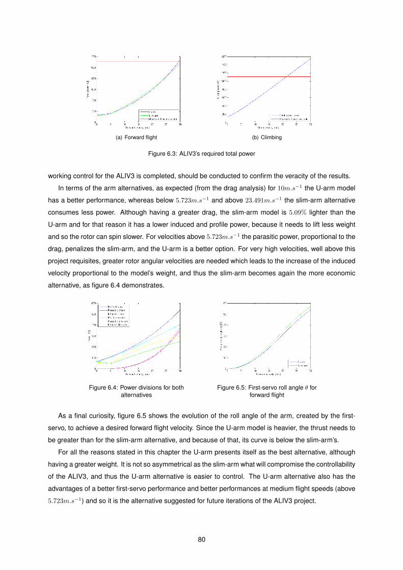
(a) Forward flight (b) Climbing

Figure 6.3: ALIV3’s required total power

working control for the ALIV3 is completed, should be conducted to confirm the veracity of the results.

In terms of the arm alternatives, as expected (from the drag analysis) for 10m.s−1 the U-arm model

has a better performance, whereas below 5.723m.s−1 and above 23.491m.s−1 the slim-arm alternative

consumes less power. Although having a greater drag, the slim-arm model is 5.09% lighter than the

U-arm and for that reason it has a lower induced and profile power, because it needs to lift less weight

and so the rotor can spin slower. For velocities above 5.723m.s−1 the parasitic power, proportional to the

drag, penalizes the slim-arm, and the U-arm is a better option. For very high velocities, well above this

project requisites, greater rotor angular velocities are needed which leads to the increase of the induced

velocity proportional to the model’s weight, and thus the slim-arm becomes again the more economic

alternative, as figure 6.4 demonstrates.

Figure 6.4: Power divisions for bothalternatives

Figure 6.5: First-servo roll angle θ forforward flight

As a final curiosity, figure 6.5 shows the evolution of the roll angle of the arm, created by the first-

servo, to achieve a desired forward flight velocity. Since the U-arm model is heavier, the thrust needs to

be greater than for the slim-arm alternative, and because of that, its curve is below the slim-arm’s.

For all the reasons stated in this chapter the U-arm presents itself as the best alternative, although

having a greater weight. It is not so asymmetrical as the slim-arm what will compromise the controllability

of the ALIV3, and thus the U-arm alternative is easier to control. The U-arm alternative also has the

advantages of a better first-servo performance and better performances at medium flight speeds (above

5.723m.s−1) and so it is the alternative suggested for future iterations of the ALIV3 project.

80

Chapter 7

Conclusions

The major achievement of the present work was the construction, for a future control system devel-

opment, of a quadrotor platform with multiple degrees of freedom, the ALIV3, theoretically capable of

moving in all six degrees of freedom maintaining its central core perfectly levelled due to the rotation of

two opposed rotors in two directions other than their rotation, and thus having the advantage of drag

reduction in comparison with standard quadrotors, because in all translations the surface facing the

airflow is independent of its velocity, and can be maximized to reduce forward drag, while for standard

quadrotors, its velocity is proportional to a roll or pitch angle of all the quadrotor. This theoretical move-

ment capacity was also fully determined with all translations and transient rebalancing operations fully

described for a perfect future control software for the ALIV3’s flight operations.

The aim of this project was to design and construct the inovative concept of a quadrotor with two

tilting rotors, the ALIV3, with the technical capacity available, and so all the necessary parts were built

with an high tenacity carbon fibre laminated composite, with a safety factor of 2 in accordance with the

Tsai-Wu failure criteria and a maximum deflection of 5mm for every part individually, and all final parts

respected this criteria.

A genetic algorithm with the blade element momentum theory was used to create an optimum ro-

tor for the ALIV3’s hovering scenario. All the necessary variables for a rapid prototyping process of a

real model were determined as well as the rotor’s ideal aerofoil. In terms of the off-the-shelf compo-

nents, several market alternatives for avionics, motors, servos and simple structural components were

evaluated and selected according to existent quadrotors, need of the project and price.

Two final models were developed, yet they only differed in the swivel arm’s format, and so only one

central area and landing gear were created, while two of each arm models were constructed, the U-arm

and the slim-arm. The U-arm is the symmetrical U-shaped, stronger swivel arm alternative, while the

slim-arm in the lighter and more simply constructed version constructed with three small carbon tubes

and connecting elbows. However after construction and testing of both alternatives, the U-arm proved

to be the best option for the ALIV3.

The final dimensions of the ALIV3 in the U-arm configuration are 620 × 642 × 245mm with 600mm

between opposed rotors and a final total weight of 1749g.

81

7.1 Future Work

In a future continuation of this project a revision of the total weight could be important but not manda-

tory, and so was proved by the small testing accident. Nevertheless the central stainless steel material

could be replaced by aluminium to decrease 65.65% of weight in those components alone. In terms of

the remaining components an optimization with reduction of material could also be studied, especially in

the arm and landing gear. The skirt tube connectors could also be improved in case of necessity, adding

two more strips, 90o from the existent ones.

The cover studied in this work was not optimized for any other direction than forward flight, and pro-

vided good results, however for the other direction the results were penalized and the cover hypothesis

is for that reason eliminated. It would be interesting, as an optimization process to design a cover that

would increase the performances in all directions, not just forward flight.

All these aspects are purely accessory, and would only improve the endurance of the ALIV3, the

crucial aspect of a continuation of this project is the ALIV3’s control implementation, because without it,

an aircraft such as this cannot fly, and that is the the most important factor in all aircraft projects.

Finally, and after a true control platform is fully functional, the transition of the ALIV3 to a UAV would

be the final iteration of this project.

82

Bibliography

[1] J. Gordon Leishman. The breguet-richet quad-rotor helicopter of 1907. www.enae.umd.edu/AGRC/

Aero/Breguet.pdf, May 2002.

[2] University of Maryland. The gamera project, 2011.

[3] Oemichen 1922. http://aviastar.org/helicopters eng/oemichen.php, February 2011.

[4] De bothezat 1922. http://aviastar.org/helicopters eng/bothezat.php, February 2011.

[5] Markman G. Holder, Steve G. Holder, and William G. Holder. Straight Up: A History of Vertical

Flight. Schiffer military/aviation history, 2000.

[6] C.Gablehouse. Helicopters and autogiros, 1969.

[7] Beating gravity - curtiss-wright x-19a. http://www.unrealaircraft.com/gravity/cw x19a.php, February

2011.

[8] Ilan Kroo, Fritz Prinz, Michael Shantz, Peter Kunz, Gary Fay, Shelley Cheng, Tibor Fabian, and

Chad Partridge. The mesicopter: A miniature rotorcraft concept - phase 2 interim report. Stanford

University, July 2000.

[9] Haomiao Huang, Gabriel M. Hoffmann, Steven L. Waslander, and Claire J. Tomlin. Aerodynamics

and control of autonomous quadrotor helicopters in aggressive maneuvering. In Proc. of the IEEE

International Conference on Robotics and Automation Guidance, Navigation, and Control Confer-

ence, 2009.

[10] Jorge Miguel Brito Domingues. Quadrotor prototipe. Master’s thesis, Instituto Superior Tecnico,

2009.

[11] Bernardo Sousa Machado Henriques. Estimation and control of a quadrotor attitude. Master’s

thesis, Instituto Superior Tecnico, 2011.

[12] Beating gravity - curtiss-wright x-19a. http://www.uavision.com/index.php?option=com content

&viewarticle&id56&Itemid37&langen, February 2011.

[13] Draganflyer x4 helicopter tech specs. http://www.draganfly.com/uav-helicopter/draganflyer-x4/

specifications/, October 2010.

83

[14] Parrot ar.drone. http://ardrone.parrot.com/parrot-ar-drone/usa/, February 2011.

[15] Arduino-based autopilot for mulitrotor craft, from quadcopters to traditional helis.

http://code.google.com/p/arducopter/wiki/ArduCopter, February 2011.

[16] Frank Colucci. The mono tiltrotor. Vertiflite, 57(2):20–23, Summer 2011.

[17] Wind tunnel testing completed on bell boeing quad tiltrotor. http://www.helis.com/news/2006/quad

windtunnel.htm, September 2006.

[18] Filipe M. S. Pedro. Projecto preliminar de um quadrirotor. Master’s thesis, Instituto Superior

Tecnico, 2009.

[19] Severino M. O. Raposo. System and process of vector propulsion with independent control of three

translation and three rotation axis. Intellectual Property, 2010.

[20] J. Gordon Leishman. Principles of Helicopter Aerodynamics. Cambridge University Press, 2000.

[21] Warren R. Young. The Helicopters. ”The Epic of Flight”. Chicago: Time-Life Books, 1982.

[22] Paul Pounds, Robert Mahony, Joel Gresham, Peter Corke, and Jonathan Roberts. Towards

dynamically-favourable quad-rotor aerial robots. Canberra, Autralia, 2004. In Proc. of Australasian

Conference on Robotics and Automation.

[23] Sergio Eduardo Aurelio Pereira da Costa. Controlo e simulacao de um quadrirotor convencional.

Master’s thesis, Instituto Superior Tecnico, 2008.

[24] Bernard Etkin and Lloyd Duff Reid. Dynamics of Flight - Stability and Control. John Wiley and

Sons, 1996.

[25] Aeroquad parts list. http://aeroquad.com/content.php?114, April 2011.

[26] Gabriel M. Hoffmann, Haomiao Huang, Steven L. Waslander, and Claire J. Tomlin. Quadrotor

helicopter flight dynamics and control: Theory and experiment. In Proc. of the AIAA Guidance,

Navigation, and Control Conference, 2007.

[27] M. Drela. Xfoil: An analysis and design system for low reynolds number airfoils. In Conference on

Low Reynolds Number Airfoil Aerodynamics. University of Notre Dame, June 1989.

[28] J. L. Hess and A. M. O. Smith. Calculation of Potential Flow About Arbitrary Bodies. Progress in

Aeronautics Sciences 8, 1967.

[29] Mark Drela and Michael B. Giles. Viscous-inviscid analysis of transonic and low reynolds number

airfoils. Aiaa Journal, 25:1347–1355, 1987.

[30] Vasco de Brederode. Fundamentos de Aerodinamica Incompressıvel. IDMEC, Instituto Superior

Tecnico, 1997.

84

[31] E. V. Laitone. Wind tunnel tests of wings at reynolds numbers below 70 000. Experiments in Fluids

23, pages 405–409, 1997.

[32] H. B. Squire, R. A. Fail, and R. C. W. Eyre. Wind-tunnel test on a 12-ft diameter helicopter rotor.

Ministry of Supply, Reports and Memoranda 2695, 1949.

[33] J. R. Meyer and G. Falabella. An investigation of the experiment aerodynamic loading on a model

helicopter rotor blade. NACA, Technical note 2953, May 1953.

[34] J. H. Holland. Adaptation in natural and artificial systems. University of Michigan Press, 1975.

[35] Kenneth Alan De Jong. An analysis of the behavior of a class of genetic adaptive systems. PhD

thesis, 1975.

[36] Alden H. Wright. Genetic algorithms for real parameter optimization. In Foundations of Genetic

Algorithms, pages 205–218. Morgan Kaufmann, 1991.

[37] Uiuc airfoil coordinates database. http://www.ae.illinois.edu/m-selig/ads/coord database.html, July

2011.

[38] Paul Pounds and Robert Mahony. Small-scale Aeroelastic Rotor Simulation, Design and Fabrica-

tion. Canberra, Australia, 2005.

[39] Antonio DiCesare Kyle Gustafson Paul Lindenfelzer. Design optimization of a quad-rotor capable

of autonomous flight. Master’s thesis, Worcester Polytechnic Institute, 2009.

[40] Samir Bouabdallah. Design and control of quadrotors with application to autonomous flying. Mas-

ter’s thesis, Ecole Polytechnique Federale de Lausanne, 2007.

[41] Find a motor. http://www.flybrushless.com/search, March 2011.

[42] J. Peraire and S. Widnall. Mit open course on dynamics, 2008. Lecture L30 -3D Rigid Body

Dynamics: Tops and Gyroscopes.

[43] Ferdinand P. Beer, Jr. E. Russell Johnston, and John T. DeWolf. Mechanical of Materials. McGraw-

Hill, 4th edition, 2006.

[44] Matweb, material property data. http://www.matweb.com/, February 2011.

[45] J. N. Reddy. Mechanics of Laminated Composite Plates and Shells: Theory and Analysis of Mate-

rials. CRC Press, 2th edition, 2003.

[46] David Roylance. Laminated Composite Plates, 2000. Department of Materials Science and Engi-

neering.

[47] ANSYS Inc. Release 12.1 documentation for ansys, 2011.

[48] J. N. Reddy. Introduction to the Finite Element Method. McGraw-Hill, 1993.

85

[49] C. M. Wang, G. T. Lim, J. N. Reddy, and K. H. Lee. Relationships between bending solutions of

reissner and mindlin plate theories. Engineering Structures, vol. 23:838–849, 2001.

[50] H. E. Rosinger and I. G. Ritchie. n timoshenko’s correction for shear in vibrating isotropic beams.

Journal of Applied Physics, vol. 10:1461–1466, 1977.

[51] Rudolph Szilard. Theory and Analysis of Plates: Classical and Numerical Methods. Prentice Hall,

1974.

[52] R. A. Serway and J. W. Jewett. Physics for Scientists and Engineers. Brooks Cole, 2004.

[53] Yvonne T. Fuchs and Karen E. Jackson. Vertical drop testing and analysis of the wasp helicopter

skid gear. Journal of the American Helicopter Society, 56(1), January 2011.

[54] J. C. F. Pereira. Mecanica dos fluidos computacional. Instituto Superior Tecnico, 2010.

[55] Doug Jackson. Aerodynamics of a helicopter rotor in forward flight, 2000.

[56] Wayne Johnson. Helicopter theory. Princeton University Press, 1980.

86

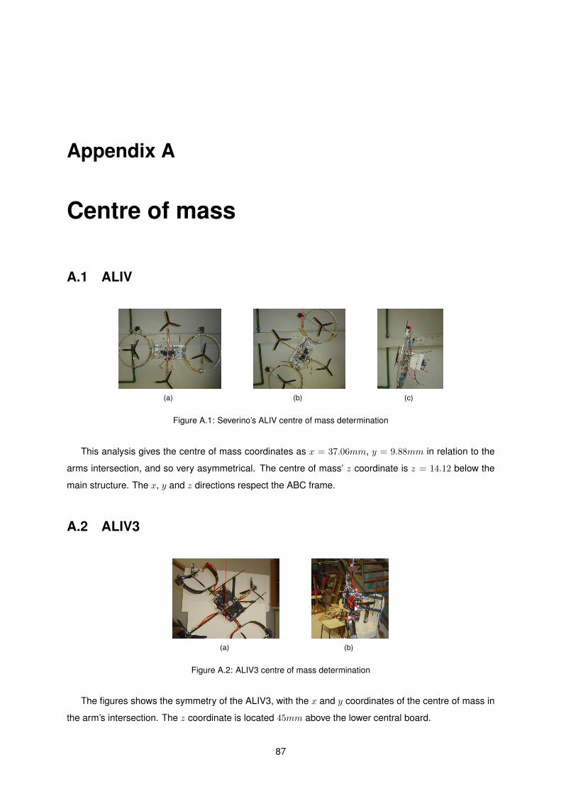
Appendix A

Centre of mass

A.1 ALIV

(a) (b) (c)

Figure A.1: Severino’s ALIV centre of mass determination

This analysis gives the centre of mass coordinates as x = 37.06mm, y = 9.88mm in relation to the

arms intersection, and so very asymmetrical. The centre of mass’ z coordinate is z = 14.12 below the

main structure. The x, y and z directions respect the ABC frame.

A.2 ALIV3

(a) (b)

Figure A.2: ALIV3 centre of mass determination

The figures shows the symmetry of the ALIV3, with the x and y coordinates of the centre of mass in

the arm’s intersection. The z coordinate is located 45mm above the lower central board.

87

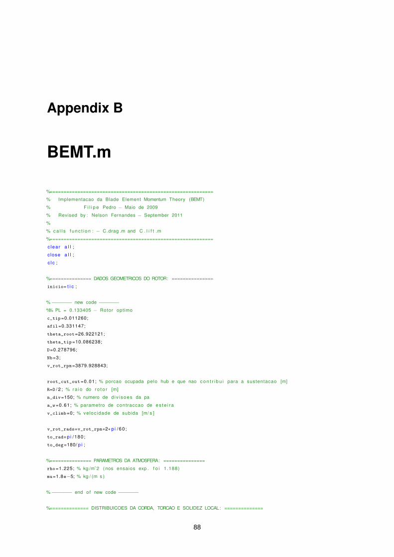
Appendix B

BEMT.m

%===========================================================

% Implementacao da Blade Element Momentum Theory (BEMT)

% F i l i p e Pedro − Maio de 2009

% Revised by : Nelson Fernandes − September 2011

%

% c a l l s f u n c t i o n : − C drag .m and C l i f t .m

%===========================================================

c lea r a l l ;

c lose a l l ;

c l c ;

%=============== DADOS GEOMETRICOS DO ROTOR: ===============

inicio= t i c ;

%−−−−−−− new code −−−−−−−

%% PL = 0.133405 − Rotor optimo

c_tip=0.011260;

afil=0.331147;

theta_root=26.922121;

theta_tip=10.086238;

D=0.278796;

Nb=3;

v_rot_rpm=3879.928843;

root_cut_out =0.01; % porcao ocupada pelo hub e que nao c o n t r i b u i para a sustentacao [m]

R=D / 2 ; % r a i o do r o t o r [m]

n_div=150; % numero de d iv i soes da pa

a_w=0.61; % parametro de contraccao de e s t e i r a

v_climb=0; % veloc idade de subida [m/ s ]

v_rot_rads=v_rot_rpm∗2∗p i / 6 0 ;

to_rad= p i /180 ;

to_deg=180/ p i ;

%=============== PARAMETROS DA ATMOSFERA: ===============

rho=1.225; % kg /mˆ2 ( nos ensaios exp . f o i 1 .188)

mu=1.8e−5; % kg / (m s )

%−−−−−−− end of new code −−−−−−−

%============== DISTRIBUICOES DA CORDA, TORCAO E SOLIDEZ LOCAL: ==============

88

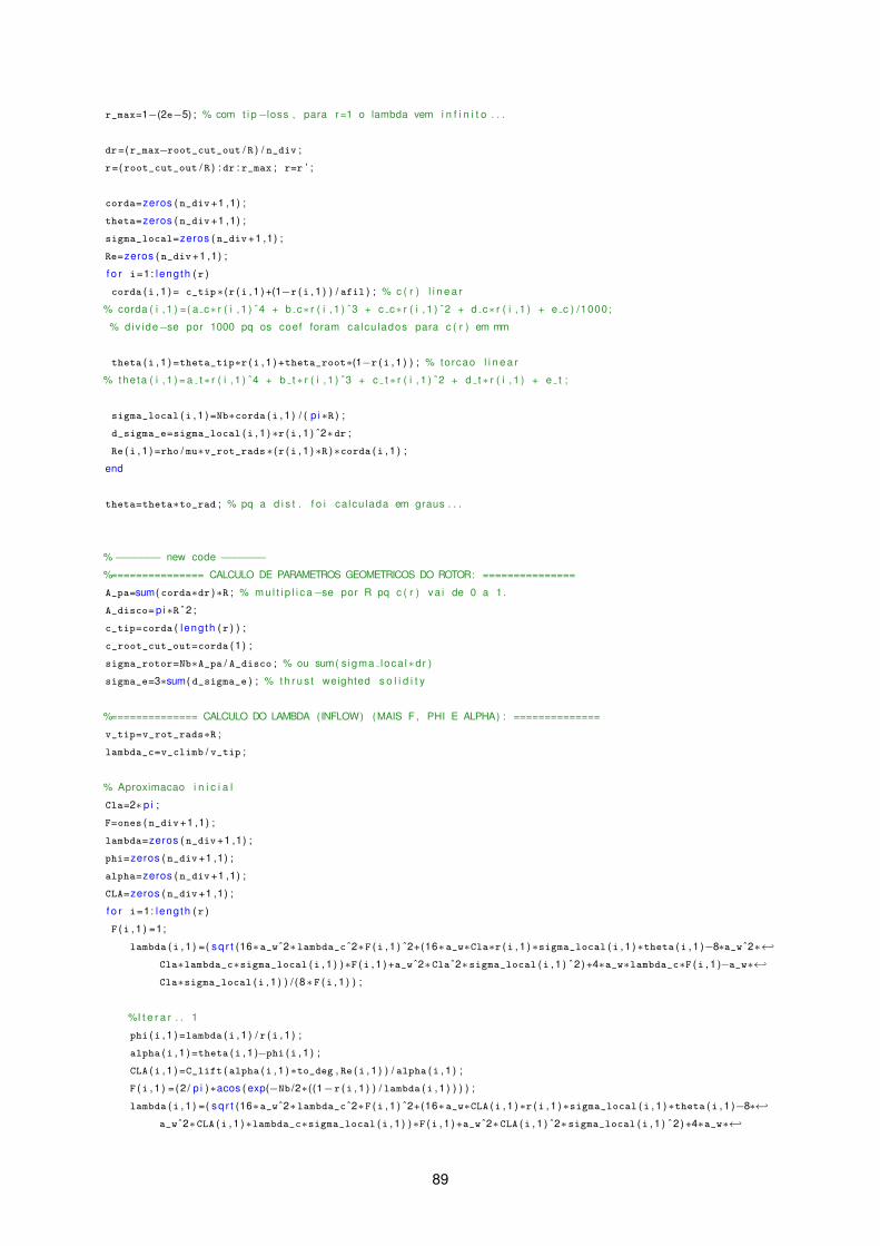
r_max=1−(2e−5) ; % com t i p−loss , para r =1 o lambda vem i n f i n i t o . . .

dr=(r_max−root_cut_out / R ) / n_div ;

r=(root_cut_out / R ) : dr : r_max ; r=r ’ ;

corda=zeros ( n_div+1 ,1) ;

theta=zeros ( n_div+1 ,1) ;

sigma_local=zeros ( n_div+1 ,1) ;

Re=zeros ( n_div+1 ,1) ;

f o r i=1: leng th ( r )

corda (i , 1 ) = c_tip∗(r (i , 1 ) +(1−r (i , 1 ) ) / afil ) ; % c ( r ) l i n e a r

% corda ( i , 1 ) =( a c∗ r ( i , 1 ) ˆ4 + b c∗ r ( i , 1 ) ˆ3 + c c∗ r ( i , 1 ) ˆ2 + d c∗ r ( i , 1 ) + e c ) /1000;

% d iv ide−se por 1000 pq os coef foram calcu lados para c ( r ) em mm

theta (i , 1 ) =theta_tip∗r (i , 1 ) +theta_root∗(1−r (i , 1 ) ) ; % torcao l i n e a r

% the ta ( i , 1 ) = a t∗ r ( i , 1 ) ˆ4 + b t∗ r ( i , 1 ) ˆ3 + c t∗ r ( i , 1 ) ˆ2 + d t∗ r ( i , 1 ) + e t ;

sigma_local (i , 1 ) =Nb∗corda (i , 1 ) / ( p i∗R ) ;

d_sigma_e=sigma_local (i , 1 )∗r (i , 1 ) ˆ2∗dr ;

Re (i , 1 ) =rho / mu∗v_rot_rads∗(r (i , 1 )∗R )∗corda (i , 1 ) ;

end

theta=theta∗to_rad ; % pq a d i s t . f o i ca lcu lada em graus . . .

%−−−−−−− new code −−−−−−−

%=============== CALCULO DE PARAMETROS GEOMETRICOS DO ROTOR: ===============

A_pa=sum( corda∗dr )∗R ; % m u l t i p l i c a−se por R pq c ( r ) va i de 0 a 1.

A_disco= p i∗R ˆ 2 ;

c_tip=corda ( leng th ( r ) ) ;

c_root_cut_out=corda ( 1 ) ;

sigma_rotor=Nb∗A_pa / A_disco ; % ou sum( s igma loca l∗dr )

sigma_e=3∗sum( d_sigma_e ) ; % t h r u s t weighted s o l i d i t y

%============== CALCULO DO LAMBDA (INFLOW) (MAIS F , PHI E ALPHA) : ==============

v_tip=v_rot_rads∗R ;

lambda_c=v_climb / v_tip ;

% Aproximacao i n i c i a l

Cla=2∗p i ;

F=ones ( n_div+1 ,1) ;

lambda=zeros ( n_div+1 ,1) ;

phi=zeros ( n_div+1 ,1) ;

alpha=zeros ( n_div+1 ,1) ;

CLA=zeros ( n_div+1 ,1) ;

f o r i=1: leng th ( r )

F (i , 1 ) =1;

lambda (i , 1 ) =( s q r t (16∗a_w ˆ2∗lambda_c ˆ2∗F (i , 1 ) ˆ2+(16∗a_w∗Cla∗r (i , 1 )∗sigma_local (i , 1 )∗theta (i , 1 )−8∗a_w ˆ2∗←

Cla∗lambda_c∗sigma_local (i , 1 ) )∗F (i , 1 ) +a_w ˆ2∗Cla ˆ2∗sigma_local (i , 1 ) ˆ 2 ) +4∗a_w∗lambda_c∗F (i , 1 )−a_w∗←

Cla∗sigma_local (i , 1 ) ) / (8∗ F (i , 1 ) ) ;

%I t e r a r . . 1

phi (i , 1 ) =lambda (i , 1 ) / r (i , 1 ) ;

alpha (i , 1 ) =theta (i , 1 )−phi (i , 1 ) ;

CLA (i , 1 ) =C_lift ( alpha (i , 1 )∗to_deg , Re (i , 1 ) ) / alpha (i , 1 ) ;

F (i , 1 ) = (2 / p i )∗acos ( exp(−Nb /2∗((1−r (i , 1 ) ) / lambda (i , 1 ) ) ) ) ;

lambda (i , 1 ) =( s q r t (16∗a_w ˆ2∗lambda_c ˆ2∗F (i , 1 ) ˆ2+(16∗a_w∗CLA (i , 1 )∗r (i , 1 )∗sigma_local (i , 1 )∗theta (i , 1 )−8∗←

a_w ˆ2∗CLA (i , 1 )∗lambda_c∗sigma_local (i , 1 ) )∗F (i , 1 ) +a_w ˆ2∗CLA (i , 1 ) ˆ2∗sigma_local (i , 1 ) ˆ 2 ) +4∗a_w∗←

89

lambda_c∗F (i , 1 )−a_w∗CLA (i , 1 )∗sigma_local (i , 1 ) ) / (8∗ F (i , 1 ) ) ;

%I t e r a r . . 2

phi (i , 1 ) =lambda (i , 1 ) / r (i , 1 ) ;

alpha (i , 1 ) =theta (i , 1 )−phi (i , 1 ) ;

CLA (i , 1 ) =C_lift ( alpha (i , 1 )∗to_deg , Re (i , 1 ) ) / alpha (i , 1 ) ;

F (i , 1 ) = (2 / p i )∗acos ( exp(−Nb /2∗((1−r (i , 1 ) ) / lambda (i , 1 ) ) ) ) ;

lambda (i , 1 ) =( s q r t (16∗a_w ˆ2∗lambda_c ˆ2∗F (i , 1 ) ˆ2+(16∗a_w∗CLA (i , 1 )∗r (i , 1 )∗sigma_local (i , 1 )∗theta (i , 1 )−8∗←

a_w ˆ2∗CLA (i , 1 )∗lambda_c∗sigma_local (i , 1 ) )∗F (i , 1 ) +a_w ˆ2∗CLA (i , 1 ) ˆ2∗sigma_local (i , 1 ) ˆ 2 ) +4∗a_w∗←

lambda_c∗F (i , 1 )−a_w∗CLA (i , 1 )∗sigma_local (i , 1 ) ) / (8∗ F (i , 1 ) ) ;

%I t e r a r . . 3

phi (i , 1 ) =lambda (i , 1 ) / r (i , 1 ) ;

alpha (i , 1 ) =theta (i , 1 )−phi (i , 1 ) ;

CLA (i , 1 ) =C_lift ( alpha (i , 1 )∗to_deg , Re (i , 1 ) ) / alpha (i , 1 ) ;

F (i , 1 ) = (2 / p i )∗acos ( exp(−Nb /2∗((1−r (i , 1 ) ) / lambda (i , 1 ) ) ) ) ;

lambda (i , 1 ) =( s q r t (16∗a_w ˆ2∗lambda_c ˆ2∗F (i , 1 ) ˆ2+(16∗a_w∗CLA (i , 1 )∗r (i , 1 )∗sigma_local (i , 1 )∗theta (i , 1 )−8∗←

a_w ˆ2∗CLA (i , 1 )∗lambda_c∗sigma_local (i , 1 ) )∗F (i , 1 ) +a_w ˆ2∗CLA (i , 1 ) ˆ2∗sigma_local (i , 1 ) ˆ 2 ) +4∗a_w∗←

lambda_c∗F (i , 1 )−a_w∗CLA (i , 1 )∗sigma_local (i , 1 ) ) / (8∗ F (i , 1 ) ) ;

end

%=============== INTEGRACAO NUMERICA DE C T , C Pi E C P0 : ===============

dCT=zeros ( n_div+1 ,1) ;

dCPi=zeros ( n_div+1 ,1) ;

dCP0=zeros ( n_div+1 ,1) ;

f o r i=1: leng th ( r )

dCT (i , 1 ) = F (i , 1 ) ∗2/a_w∗lambda (i , 1 ) ∗(lambda (i , 1 )−a_w∗lambda_c )∗r (i , 1 )∗dr ;

dCPi (i , 1 ) = lambda (i , 1 )∗dCT (i , 1 ) ;

dCP0 (i , 1 ) = sigma_local (i , 1 ) /2∗C_drag ( alpha (i , 1 )∗to_deg , Re (i , 1 ) ) ∗(r (i , 1 ) ) ˆ3∗dr ;

end

C_T=sum( dCT ) ;

C_Pi=sum( dCPi ) ;

C_P0=sum( dCP0 ) ;

C_P=C_Pi+C_P0 ;

%−−−−−−− end of new code −−−−−−−

%=============== CALCULOS DA PERFORMANCE: ===============

disp ( ’ Performance : ’ )

k=C_Pi∗ s q r t (4∗a_w ) / C_T ˆ ( 3 / 2 ) ;

FM=C_T ˆ ( 3 / 2 ) / ( s q r t (4∗a_w )∗C_P ) ;

PL=C_T / ( C_P∗v_tip ) ;

T=C_T∗rho∗A_disco∗v_tip ˆ 2 ;

P=C_P∗rho∗A_disco∗v_tip ˆ 3 ;

f p r i n t f ( ’ Para V ro t = %d rpm:\nT = %f g\nT = %f N\nP = %f W\nPL = %f\nCT = %f\nCP = %f\n ’ , v_rot_rpm , T←

/9 .81∗1e3 , T , P , PL , C_T , C_P )

rpm=0:100:12000; rpm=rpm ’ ;

omega=rpm∗2∗p i / 6 0 ;

f o r i=1: leng th ( omega )

PL_curva (i , 1 ) =C_T / ( omega (i , 1 )∗R∗C_P ) ;

T_curva (i , 1 ) =C_T∗rho∗A_disco∗R ˆ2∗omega (i , 1 ) ˆ 2 ;

P_curva (i , 1 ) =C_P∗rho∗A_disco∗R ˆ3∗omega (i , 1 ) ˆ 3 ;

end

90

Appendix C

GA.m

%=======================================================================================

% ALGORITMO GENETICO

% F i l i p e Pedro − Junho 2009

% Revised by : Nelson Fernandes − September 2011

% Cr ia os f i c h e i r o s : − ga resu l tados . dat e ga condicoes . dat

%=======================================================================================

c lea r a l l

c lose a l l

c l c

%=============== PARAMETROS: ===============

disp ( round ( c lock ) )

d isp ( ’−−−−−−−−−−−−−−−−−−−−−−−−−−−−−−ALGORITMO−GENETICO−−−−−−−−−−−−−−−−−−−−−−−−−−−−−−−− ’ )

n_gen= inpu t ( ’ numero de geracoes = ’ ) ; % numero maximo de geracoes

n_pop= inpu t ( ’ tamanho da populacao = ’ ) ; % numero de i n d i v i d u o s na populacao

pop_keep= inpu t ( ’ percentagem da pop . a manter [ 0 : 1 ] = ’ ) ; % percentagem da populacao a manter

n_keep=round ( pop_keep∗n_pop ) ;

f p r i n t f ( ’=> n keep = %d\n ’ , n_keep )

i f mod ( n_keep , 2 ) % v e r i f i c a c a o se n keep par :

d isp ( ’ ERRO ! ! ! \n Ajus te pop keep ou n pop de forma a n keep ser par ! ’ )

break

end

taxa_mut= inpu t ( ’ taxa de mutacao [ 0 : 1 ] = ’ ) ; % taxa de mutacao

disp ( ’−−−−−−−−−−−−−−−−−−−−−−−−−−−−−−−−−−−−−−−−−−−−−−−−−−−−−−−−−−−−−−−−−−−−−−−−−−−−−−−− ’ )

metodo_selec=menu( ’ Metodo de Seleccao : ’ , ’ Ranking ’ , ’ Rou le t te Wheel ’ , ’ Torneio ’ ) ;

metodo_empar=menu( ’ Metodo de Emparelhamento : ’ , ’ Adjacent F i tness Pa i r i ng ’ , ’ Best−Mate−Worst ’ ) ;

metodo_cross=menu( ’ Metodo de Acasalamento : ’ , ’ A r i t h m e t i c Crossover ’ , ’ I n te rmed ia te Crossover ’ ) ;

d isp ( ’−−−−−−−−−−−−−−−−−−−−−−−−−−−−−−−−−−−−−−−−−−−−−−−−−−−−−−−−−−−−−−−−−−−−−−−−−−−−−−−− ’ )

% vectores com os va lo res max e min dos parametros ( param 1 , param 2 , . . . , param n ) :

param=[ ’ c t i p ’ ; ’ lambda ’ ; ’ t r o o t ’ ; ’ t e t i p ’ ; ’ DD ’ ; ’ Nb ’ ; ’ rotrpm ’ ] ;

tipo=[ ’ r e a l ’ ; ’ r e a l ’ ; ’ r e a l ’ ; ’ r e a l ’ ; ’ r e a l ’ ; ’ i n t r ’ ; ’ r e a l ’ ] ; % todas estas s t r i n g s tem de t e r o mesmo ←

comprimento ! ! !

param_min = [0 ,0 .3 ,0 ,0 ,0 .1 ,2 ,2000 ] ;

param_max =[0 .015 ,1 ,30 ,30 ,0 .279 ,4 ,10000] ;

% r e s t r i c o e s :

T_min=4;

P_max=100;

i f l eng th ( param_min ) ˜= leng th ( param_max )

d isp ( ’ l i m i t e s de parametros mal i n t r oduz i dos ! ’ )

break

91

else

n_param= leng th ( param_min ) ;

end

disp ( ’ Parametro : \ t \ tT ipo :\ tGama de va lo res poss i ve l :\n ’ )

f o r i=1:n_param

f p r i n t f ( ’%s \ t−>\t%s\ t [% f : %f ]\n ’ , param (i , : ) , tipo (i , : ) , param_min ( i ) , param_max ( i ) )

end

disp ( ’−−−−−−−−−−−−−−−−−−−−−−−−−−−−−−−−−−−−−−−−−−−−−−−−−−−−−−−−−−−−−−−−−−−−−−−−−−−−−−−− ’ )

d isp ( ’ Rest r icoes : ’ )

f p r i n t f ( ’ T min = %f\nP max = %f\n ’ ,T_min , P_max )

d isp ( ’−−−−−−−−−−−−−−−−−−−−−−−−−−−−−−−−−−−−−−−−−−−−−−−−−−−−−−−−−−−−−−−−−−−−−−−−−−−−−−−− ’ )

save ( ’ . / ga condicoes . dat ’ , ’ n gen ’ , ’ n pop ’ , ’ pop keep ’ , ’ n keep ’ , ’ taxa mut ’ , ’ metodo selec ’ , ’ metodo empar ’ , . . .

’ metodo cross ’ , ’ param ’ , ’ n param ’ , ’ t i p o ’ , ’ param min ’ , ’ param max ’ , ’ T min ’ , ’ P max ’ )

%=============== ALGORITMO: ===============

inicio= t i c ;

f p r i n t f ( ’\nNumero de ava l iacoes a e fec tua r = %d\nTempo estimado para acabar (1 s por ava l iacao ) = %5.1 f ←

horas\n ’ , . . .

n_pop+n_gen∗(n_pop−n_keep+n_pop∗n_param∗taxa_mut ) , ( n_pop+n_gen∗(n_pop−n_keep+n_pop∗n_param∗taxa_mut ) )←

∗1/60/60)

% c o n s t i t u i c a o da populacao i n i c i a l :

f o r i=1:n_param

i f strcmp ( tipo (i , : ) , ’ r e a l ’ ) % parametros rea i s

pop_inicial ( : , i ) =(param_max ( i )−param_min ( i ) )∗rand ( n_pop , 1 ) +param_min ( i ) ;

e lse % parametros i n t e i r o s

pop_inicial ( : , i ) =round ( ( param_max ( i )−param_min ( i ) )∗rand ( n_pop , 1 ) +param_min ( i ) ) ;

end

end

disp ( ’\nPopulacao i n i c i a l gerada . . . ’ )

pop=fitness ( pop_inicial , n_param , T_min , P_max ) ; % ca l cu la na u l t ima coluna a ’ f i t n e s s ’ de cada cromossoma

disp ( ’ . . . e ava l iada ! ’ )

% c i c l o de geracoes :

fid=fopen ( ’ ga resu l tados . dat ’ , ’ a ’ ) ;

versao=vers ion ;

f p r i n t f ( fid , ’ # Resultados do Algor i tmo Genetico ( c o r r i d o em Octave %s )\n# Geracao | Parametro 1 | ←

Parametro 2 | . . . | Fi tness | Media Geracao ’ , versao )

d isp ( ’\n I n i c i o do c i c l o de Geracoes . . . \ n Progresso : ’ )

f o r gen=1:n_gen

f p r i n t f ( ’ %3.1 f%% ’ ,gen / n_gen∗100)

pais=seleccao ( pop , n_keep , metodo_selec ) ; % seleccao dos cromossomas para o ’ mating ’

pais_empar=empar ( pais , metodo_empar ) ; % emparelhamento dos pais para o ’ mating ’

filhos=crossover ( pais_empar , n_pop , tipo , metodo_cross ) ; % ’ mating ’ dos pais

filhos=fitness ( filhos , n_param , T_min , P_max ) ; % determinacao da ’ f i t n e s s ’ dos f i l h o s

% mutacao dof f i l h o s :

[ fit , indice ]= min ( filhos ( : , n_param+1) ) ;

filhos=mutacao ( filhos , taxa_mut , tipo , param_min , param_max , T_min , P_max , indice ) ;

% concatenacao dos pais com os f i l h o s :

pop_nova=pais ;

[ dimm , auxxx ]= s ize ( filhos ) ;

f o r i=1:dimm

f o r j=1:n_param+1

92

pop_nova ( i+n_keep , j ) =filhos (i , j ) ;

end

end

% mutacao t o t a l =0 , para o codigo corresponder ao o r i g i n a l

[ fit , indice ]= min ( pop_nova ( : , n_param+1) ) ;

pop=mutacao ( pop_nova , 0 , tipo , param_min , param_max , T_min , P_max , indice ) ;

% Determina o melhor e a media da geracao , e guarda no f i c h e i r o ga resu l tados . dat :

[ fit , indice ]= min ( pop ( : , n_param+1) ) ;

f p r i n t f ( fid , ’\n%d ’ ,gen ) ;

f p r i n t f ( fid , ’%f %f ’ ,pop ( indice , : ) ,mean( pop ( : , n_param+1) ) ) ;

end

disp ( ’\n Calculos conc lu idos ! \n ’ )

telapsed=toc ( inicio ) ;

horas= f l o o r ( ( telapsed ) / 60 /60 ) ;

minutos= f l o o r ( ( ( telapsed ) /60/60−horas ) ∗60) ;

segundos=round ( ( ( ( telapsed ) /60/60−horas )∗60−minutos ) ∗60) ;

f p r i n t f ( ’\nO codigo demorou %f horas a c o r r e r (%d horas %d minutos e %d segundos )\n ’ , ( telapsed ) /60 /60 ,←

horas , minutos , segundos ) ;

f p r i n t f ( fid , ’\n# O codigo demorou %f minutos a c o r r e r (%d horas %d minutos e %d segundos ) ’ , ( telapsed ) /60 ,←

horas , minutos , segundos ) ;

f c l o s e ( fid ) ;

%=============== RESULTADOS: ===============

disp ( ’\nResultados F ina i s :\n ’ )

f o r i=1:n_param

f p r i n t f ( ’%s \ t−>\t%f \n ’ , param (i , : ) ,pop ( indice , i ) )

end

f p r i n t f ( ’\nFi tness F ina l = %f\n ’ ,pop ( indice , n_param+1) )

[ PL , T , P , C_T , C_P ]= f_BEMT ( pop ( indice , 1 ) ,pop ( indice , 2 ) ,pop ( indice , 3 ) ,pop ( indice , 4 ) ,pop ( indice , 5 ) ,pop ( indice←

, 6 ) ,pop ( indice , 7 ) ,0 .61 ,0 ,0 .01 ) ;

f p r i n t f ( ’\nPL = %f\nThrust = %f\nPower = %f\nC T = %f\nC P = %f\n ’ ,PL , T , P , C_T , C_P ) ;

Auxiliary functions

% FITNESS

f u n c t i o n [ m ] = fitness (m , n_param , T_min , P_max )

[ j , k ]= s ize ( m ) ;

f o r i=1:j

[ PL , T , P ]= f_BEMT ( m (i , 1 ) ,m (i , 2 ) ,m (i , 3 ) ,m (i , 4 ) ,m (i , 5 ) ,m (i , 6 ) ,m (i , 7 ) ,0 .61 ,0 ,0 .01 ) ;

% penal izacao por t h r u s t i n s u f i c i e n t e :

i f (T<T_min | | P>P_max )

penalidade=0;

e lse

penalidade=1;

end

m (i , n_param+1)=−PL∗penalidade ;

end

end

% SELECCAO: ( se lecc iona os cromossomas que se i r a o rep roduz i r )

f u n c t i o n [ escolhidos ] = seleccao ( pop , n_keep , metodo )

[ linhas , colunas ]= s ize ( pop ) ;

[ s , indice ]= s o r t ( pop ( : , colunas ) ) ;

escolhidos ( 1 , : ) =pop ( indice ( 1 ) , : ) ; % e l i t i s m o

i f metodo==1 % OPCAO 1−> Seleccao por ’ ranking ’

93

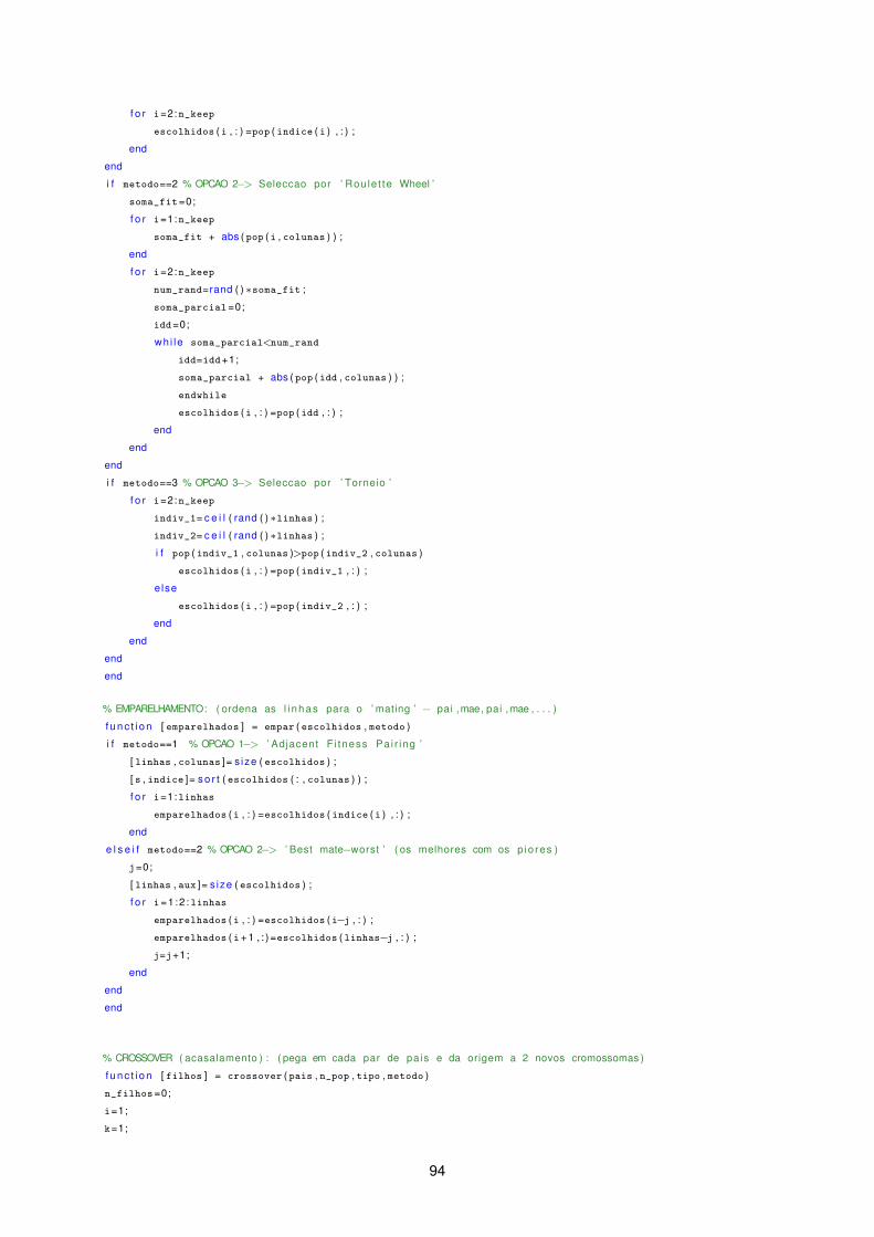
f o r i=2:n_keep

escolhidos (i , : ) =pop ( indice ( i ) , : ) ;

end

end

i f metodo==2 % OPCAO 2−> Seleccao por ’ Rou le t te Wheel ’

soma_fit=0;

f o r i=1:n_keep

soma_fit + abs ( pop (i , colunas ) ) ;

end

f o r i=2:n_keep

num_rand=rand ( ) ∗soma_fit ;

soma_parcial=0;

idd=0;

wh i le soma_parcial<num_rand

idd=idd+1;

soma_parcial + abs ( pop ( idd , colunas ) ) ;

endwhile

escolhidos (i , : ) =pop ( idd , : ) ;

end

end

end

i f metodo==3 % OPCAO 3−> Seleccao por ’ Torneio ’

f o r i=2:n_keep

indiv_1= c e i l ( rand ( ) ∗linhas ) ;

indiv_2= c e i l ( rand ( ) ∗linhas ) ;

i f pop ( indiv_1 , colunas )>pop ( indiv_2 , colunas )

escolhidos (i , : ) =pop ( indiv_1 , : ) ;

e lse

escolhidos (i , : ) =pop ( indiv_2 , : ) ;

end

end

end

end

% EMPARELHAMENTO: ( ordena as l i n h a s para o ’ mating ’ − pai ,mae, pai ,mae , . . . )

f u n c t i o n [ emparelhados ] = empar ( escolhidos , metodo )

i f metodo==1 % OPCAO 1−> ’ Adjacent F i tness Pa i r ing ’

[ linhas , colunas ]= s ize ( escolhidos ) ;

[ s , indice ]= s o r t ( escolhidos ( : , colunas ) ) ;

f o r i=1:linhas

emparelhados (i , : ) =escolhidos ( indice ( i ) , : ) ;

end

e l s e i f metodo==2 % OPCAO 2−> ’ Best mate−worst ’ ( os melhores com os p io res )

j=0;

[ linhas , aux ]= s ize ( escolhidos ) ;

f o r i=1:2 : linhas

emparelhados (i , : ) =escolhidos (i−j , : ) ;

emparelhados ( i+1 , : ) =escolhidos ( linhas−j , : ) ;

j=j+1;

end

end

end

% CROSSOVER ( acasalamento ) : ( pega em cada par de pais e da origem a 2 novos cromossomas )

f u n c t i o n [ filhos ] = crossover ( pais , n_pop , tipo , metodo )

n_filhos=0;

i=1;

k=1;

94

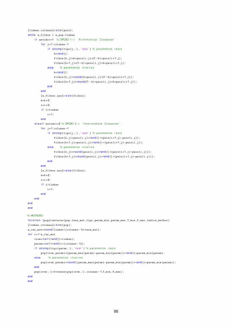
[ linhas , colunas ]= s ize ( pais ) ;

wh i le n_filhos < n_pop−linhas

i f metodo==1 % OPCAO 1−> ’ A r i t h m e t i c a l Crossover ’

f o r j=1:colunas−1

i f strcmp ( tipo (j , : ) , ’ r e a l ’ ) % parametros rea i s

b=rand ( ) ;

filhos (k , j ) =b∗pais (i , j ) +(1−b )∗pais ( i+1 ,j ) ;

filhos ( k+1 ,j ) =(1−b )∗pais (i , j ) +b∗pais ( i+1 ,j ) ;

e lse % parametros i n t e i r o s

b=rand ( ) ;

filhos (k , j ) =round ( b∗pais (i , j ) +(1−b )∗pais ( i+1 ,j ) ) ;

filhos ( k+1 ,j ) =round((1−b )∗pais (i , j ) +b∗pais ( i+1 ,j ) ) ;

end

end

[ n_filhos , aux ]= s ize ( filhos ) ;

k=k+2;

i=i+2;

i f i>linhas

i=1;

end

e l s e i f metodo==2 % OPCAO 2−> ’ I n te rmed ia te Crossover ’

f o r j=1:colunas−1

i f strcmp ( tipo (j , : ) , ’ r e a l ’ ) % parametros rea i s

filhos (k , j ) =pais (i , j ) +rand ( ) ∗(pais ( i+1 ,j )−pais (i , j ) ) ;

filhos ( k+1 ,j ) =pais (i , j ) +rand ( ) ∗(pais ( i+1 ,j )−pais (i , j ) ) ;

e lse % parametros i n t e i r o s

filhos (k , j ) =round ( pais (i , j ) +rand ( ) ∗(pais ( i+1 ,j )−pais (i , j ) ) ) ;

filhos ( k+1 ,j ) =round ( pais (i , j ) +rand ( ) ∗(pais ( i+1 ,j )−pais (i , j ) ) ) ;

end

end

[ n_filhos , aux ]= s ize ( filhos ) ;

k=k+2;

i=i+2;

i f i>linhas

i=1;

end

end

end

end

% MUTACAO:

f u n c t i o n [ pop ]= mutacao ( pop , taxa_mut , tipo , param_min , param_max , T_min , P_max , indice_melhor )

[ linhas , colunas ]= s ize ( pop ) ;

n_var_mut=round ( linhas∗(colunas−1)∗taxa_mut ) ;

f o r i=1:n_var_mut

crom= c e i l ( rand ( ) ∗linhas ) ;

param= c e i l ( rand ( ) ∗(colunas−1) ) ;

i f strcmp ( tipo ( param , : ) , ’ r e a l ’ ) % parametros rea i s

pop ( crom , param ) =(param_max ( param )−param_min ( param ) )∗rand ( ) +param_min ( param ) ;

e lse % parametros i n t e i r o s

pop ( crom , param ) =round ( ( param_max ( param )−param_min ( param ) )∗rand ( ) +param_min ( param ) ) ;

end

pop ( crom , : ) =fitness ( pop ( crom , : ) , colunas−1,T_min , P_max ) ;

end

end

95

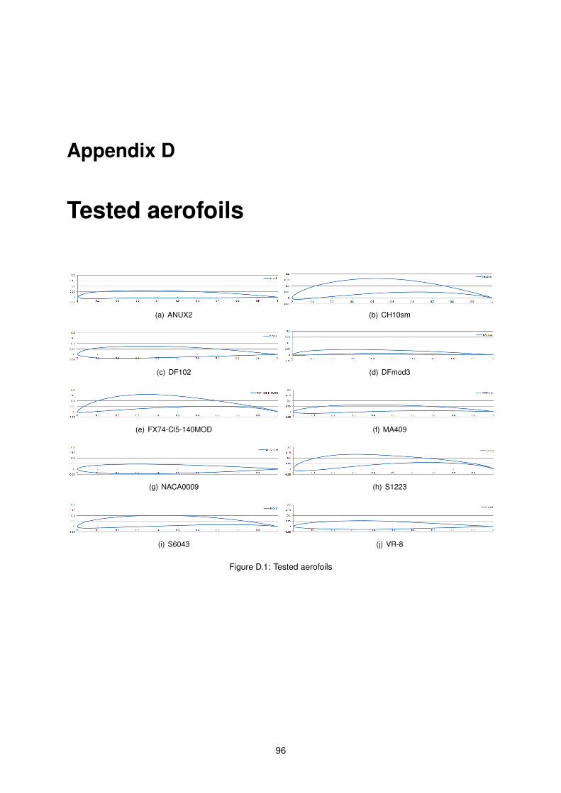
Appendix D

Tested aerofoils

(a) ANUX2 (b) CH10sm

(c) DF102 (d) DFmod3

(e) FX74-Cl5-140MOD (f) MA409

(g) NACA0009 (h) S1223

(i) S6043 (j) VR-8

Figure D.1: Tested aerofoils

96

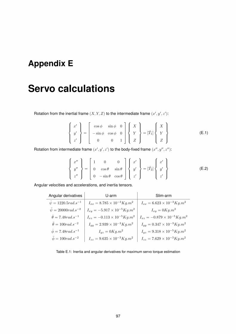
Appendix E

Servo calculations

Rotation from the inertial frame (X,Y, Z) to the intermediate frame (x′, y′, z′):

x′

y′

z′

=

cosφ sinφ 0

− sinφ cosφ 0

0 0 1

X

Y

Z

= [T1]

X

Y

Z

(E.1)

Rotation from intermediate frame (x′, y′, z′) to the body-fixed frame (x′′, y′′, z′′):

x′′

y′′

z′′

=

1 0 0

0 cos θ sin θ

0 − sin θ cos θ

x′

y′

z′

= [T2]

x′

y′

z′

(E.2)

Angular velocities and accelerations, and inertia tensors.

Angular derivatives U-arm Slim-arm

ψ = 1220.5rad.s−1 Ixx = 8.785× 10−3Kg.m2 Ixx = 6.623× 10−3Kg.m2

ψ = 20000rad.s−2 Ixy = −5.917× 10−5Kg.m2 Ixy = 0Kg.m2

θ = 7.48rad.s−1 Ixz = −0.113× 10−5Kg.m2 Ixz = −0.879× 10−5Kg.m2

θ = 100rad.s−2 Iyy = 2.939× 10−3Kg.m2 Iyy = 0.347× 10−3Kg.m2

φ = 7.48rad.s−1 Iyz = 0Kg.m2 Iyz = 9.318× 10−5Kg.m2

φ = 100rad.s−2 Izz = 9.635× 10−3Kg.m2 Izz = 7.629× 10−3Kg.m2

Table E.1: Inertia and angular derivatives for maximum servo torque estimation

97

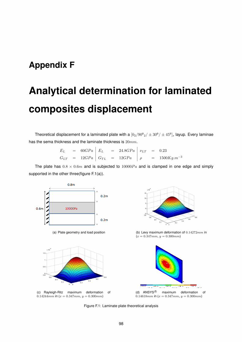
Appendix F

Analytical determination for laminated

composites displacement

Theoretical displacement for a laminated plate with a [02/90o2/± 30o/± 45o]s layup. Every laminae

has the sema thickness and the laminate thickness is 20mm.

EL = 60GPa EL = 24.8GPa νLT = 0.23

GLT = 12GPa GTL = 12GPa ρ = 1500Kg.m−3

The plate has 0.8 × 0.6m and is subjected to 10000Pa and is clamped in one edge and simply

supported in the other three(figure F.1(a)).

(a) Plate geometry and load position (b) Levy maximum deformation of 0.14272mm in(x = 0.347mm, y = 0.300mm)

(c) Rayleigh-Ritz maximum deformation of0.14244mm in (x = 0.347mm, y = 0.300mm)

(d) ANSYS R© maximum deformation of0.14618mm in (x = 0.347mm, y = 0.300mm)

Figure F.1: Laminate plate theoretical analysis

98

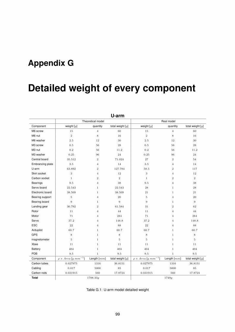
Appendix G

Detailed weight of every component

U-armTheoretical model Real model

Component weight [g] quantity total weight [g] weight [g] quantity total weight [g]

M6 screw 15 4 60 15 4 60

M6 nut 2 8 16 2 8 16

M6 washer 2.5 12 30 2.5 12 30

M3 screw 0.5 56 28 0.5 56 28

M3 nut 0.2 56 11.2 0.2 56 11.2

M3 washer 0.25 96 24 0.25 96 24

Central board 35.512 2 71.024 27 2 54

Embrancing plate 3.5 4 14 3.5 4 14

U-arm 63.892 2 127.784 58.5 2 117

Skirt socket 3 4 12 3 4 12

Carbon socket 1 2 2 1 2 2

Bearings 9.5 4 38 9.5 4 38

Servo board 22.543 1 22.543 28 1 28

Electronic board 38.509 1 38.509 21 1 21

Bearing support 5 4 20 5 4 20

Bearing board 9 1 9 9 1 9

Landing gear 30.792 2 61.584 31 2 62

Rotor 11 4 44 11 4 44

Motor 71 4 284 71 4 284

Servo 37.2 4 148.8 37.2 4 148.8

ESC 22 4 88 22 4 88

Ardupilot 60.7 1 60.7 60.7 1 60.7

GPS 8 1 8 8 1 8

magnetometer 5 1 5 5 1 5

Xbee 11 1 11 11 1 11

Battery 404 1 404 404 1 404

PDB 9.5 1 9.5 9.5 1 9.5

Component ρ× Area [g.mm−1] Length [mm] total weight [g] ρ× Area [g.mm−1] Length [mm] total weight [g]

Carbon tubes 0.027975 1316 36.8151 0.027975 1316 36.8151

Cabling 0.017 5000 85 0.017 5000 85

Carbon rods 0.031915 560 17.8724 0.031915 560 17.8724

Total 1788.33g 1749g

Table G.1: U-arm model detailed weight

99

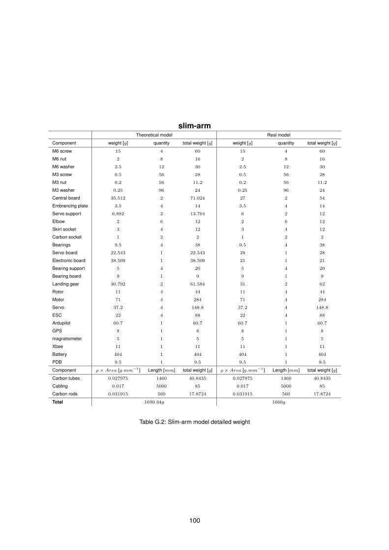
slim-armTheoretical model Real model

Component weight [g] quantity total weight [g] weight [g] quantity total weight [g]

M6 screw 15 4 60 15 4 60

M6 nut 2 8 16 2 8 16

M6 washer 2.5 12 30 2.5 12 30

M3 screw 0.5 56 28 0.5 56 28

M3 nut 0.2 56 11.2 0.2 56 11.2

M3 washer 0.25 96 24 0.25 96 24

Central board 35.512 2 71.024 27 2 54

Embrancing plate 3.5 4 14 3.5 4 14

Servo support 6.882 2 13.764 6 2 12

Elbow 2 6 12 2 6 12

Skirt socket 3 4 12 3 4 12

Carbon socket 1 2 2 1 2 2

Bearings 9.5 4 38 9.5 4 38

Servo board 22.543 1 22.543 28 1 28

Electronic board 38.509 1 38.509 21 1 21

Bearing support 5 4 20 5 4 20

Bearing board 9 1 9 9 1 9

Landing gear 30.792 2 61.584 31 2 62

Rotor 11 4 44 11 4 44

Motor 71 4 284 71 4 284

Servo 37.2 4 148.8 37.2 4 148.8

ESC 22 4 88 22 4 88

Ardupilot 60.7 1 60.7 60.7 1 60.7

GPS 8 1 8 8 1 8

magnetometer 5 1 5 5 1 5

Xbee 11 1 11 11 1 11

Battery 404 1 404 404 1 404

PDB 9.5 1 9.5 9.5 1 9.5

Component ρ× Area [g.mm−1] Length [mm] total weight [g] ρ× Area [g.mm−1] Length [mm] total weight [g]

Carbon tubes 0.027975 1460 40.8435 0.027975 1460 40.8435

Cabling 0.017 5000 85 0.017 5000 85

Carbon rods 0.031915 560 17.8724 0.031915 560 17.8724

Total 1690.34g 1660g

Table G.2: Slim-arm model detailed weight

100