The Stereology Workstation - unifr.ch · The Stereology Workstation By Jon Ekman. Start-up 1. Turn MASTER switch on Belkin Surge-Master. This will turn on the LUDL stage controller,

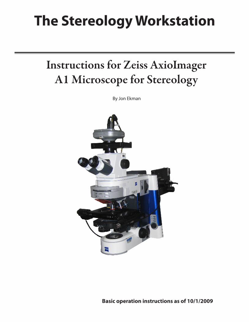
Instructions for Zeiss AxioImager A1 Microscope for Stereology

Basic operation instructions as of 10/1/2009

The Stereology Workstation

By Jon Ekman

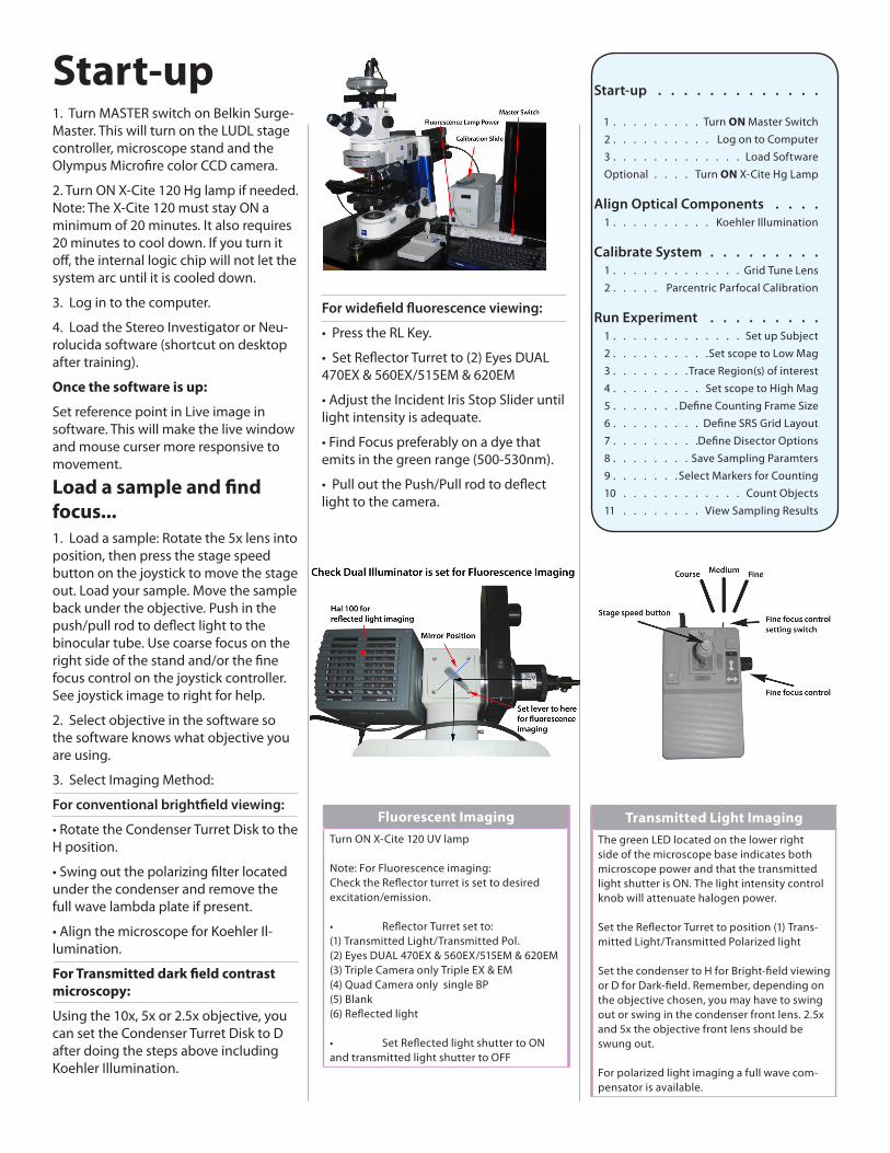
Start-up1. Turn MASTER switch on Belkin Surge-Master. This will turn on the LUDL stage controller, microscope stand and the Olympus Microfire color CCD camera.

2. Turn ON X-Cite 120 Hg lamp if needed. Note: The X-Cite 120 must stay ON a minimum of 20 minutes. It also requires 20 minutes to cool down. If you turn it off, the internal logic chip will not let the system arc until it is cooled down.

3. Log in to the computer.

4. Load the Stereo Investigator or Neu-rolucida software (shortcut on desktop after training).

Once the software is up:

Set reference point in Live image in software. This will make the live window and mouse curser more responsive to movement.

Load a sample and find focus...1. Load a sample: Rotate the 5x lens into position, then press the stage speed button on the joystick to move the stage out. Load your sample. Move the sample back under the objective. Push in the push/pull rod to deflect light to the binocular tube. Use coarse focus on the right side of the stand and/or the fine focus control on the joystick controller. See joystick image to right for help.

2. Select objective in the software so the software knows what objective you are using.

3. Select Imaging Method:

For conventional brightfield viewing:

• Rotate the Condenser Turret Disk to the H position.

• Swing out the polarizing filter located under the condenser and remove the full wave lambda plate if present.

• Align the microscope for Koehler Il-lumination.

For Transmitted dark field contrast microscopy:

Using the 10x, 5x or 2.5x objective, you can set the Condenser Turret Disk to D after doing the steps above including Koehler Illumination.

For widefield fluorescence viewing:

• Press the RL Key.

• Set Reflector Turret to (2) Eyes DUAL 470EX & 560EX/515EM & 620EM

• Adjust the Incident Iris Stop Slider until light intensity is adequate.

• Find Focus preferably on a dye that emits in the green range (500-530nm).

• Pull out the Push/Pull rod to deflect light to the camera.

Start-up

1 . . . . . . . . . Turn ON Master Switch2 . . . . . . . . . . Log on to Computer3 . . . . . . . . . . . . . Load SoftwareOptional . . . . Turn ON X-Cite Hg Lamp

Align Optical Components 1 . . . . . . . . . . Koehler Illumination

Calibrate System 1 . . . . . . . . . . . . . Grid Tune Lens2 . . . . . Parcentric Parfocal Calibration

Run Experiment 1 . . . . . . . . . . . . . Set up Subject2 . . . . . . . . . .Set scope to Low Mag3 . . . . . . . . Trace Region(s) of interest4 . . . . . . . . . Set scope to High Mag5 . . . . . . . Define Counting Frame Size6 . . . . . . . . . Define SRS Grid Layout7 . . . . . . . . .Define Disector Options8 . . . . . . . . Save Sampling Paramters9 . . . . . . . Select Markers for Counting10 . . . . . . . . . . . . Count Objects11 . . . . . . . . View Sampling Results

Fluorescent ImagingTurn ON X-Cite 120 UV lamp

Note: For Fluorescence imaging: Check the Reflector turret is set to desired excitation/emission.

• Reflector Turret set to:(1) Transmitted Light/Transmitted Pol.(2) Eyes DUAL 470EX & 560EX/515EM & 620EM(3) Triple Camera only Triple EX & EM(4) Quad Camera only single BP(5) Blank(6) Reflected light

• Set Reflected light shutter to ON and transmitted light shutter to OFF

Transmitted Light Imaging The green LED located on the lower right side of the microscope base indicates both microscope power and that the transmitted light shutter is ON. The light intensity control knob will attenuate halogen power.

Set the Reflector Turret to position (1) Trans-mitted Light/Transmitted Polarized light

Set the condenser to H for Bright-field viewing or D for Dark-field. Remember, depending on the objective chosen, you may have to swing out or swing in the condenser front lens. 2.5x and 5x the objective front lens should be swung out.

For polarized light imaging a full wave com-pensator is available.

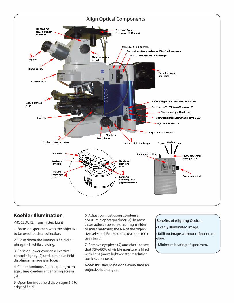
Align Optical Components

Koehler IlluminationPROCEDURE: Transmitted Light

1. Focus on specimen with the objective to be used for data collection.

2. Close down the luminous field dia-phragm (1) while viewing.

3. Raise or Lower condenser vertical control slightly (2) until luminous field diaphragm image is in focus.

4. Center luminous field diaphragm im-age using condenser centering screws (3).

5. Open luminous field diaphragm (1) to edge of field.

6. Adjust contrast using condenser aperture diaphragm slider (4). In most cases adjust aperture diaphragm slider to mark matching the NA of the objec-tive selected. For 20x, 40x, 63x and 100x use step 7.

7. Remove eyepiece (5) and check to see that 75%-80% of visible aperture is filled with light (more light=better resolution but less contrast).

Note: this should be done every time an objective is changed.

Benefits of Aligning Optics:

• Evenly illuminated image.

• Brilliant image without reflection or glare.

• Minimum heating of specimen.

CalibrationThe system is calibrated by ITG staff, and new users get these initial calibration settings at first login and startup.

The calibration is done using transmit-ted brightfield method.

Calibrate only the objectives you plan to use in your experiment.

Recalibrate only if you notice drastic errors in software contour placement between objectives.

Oil is not needed to Grid tune lenses.

Setup1. Log in to the computer.

2. Load the Stereo Investigator or Neu-rolucida software. (Shortcut on desktop after training)

3. Load the calibration grid slide. Select the 10x objective on the microscope and in the software.

4. Push in the push/pull rod to deflect light to the binocular tube.

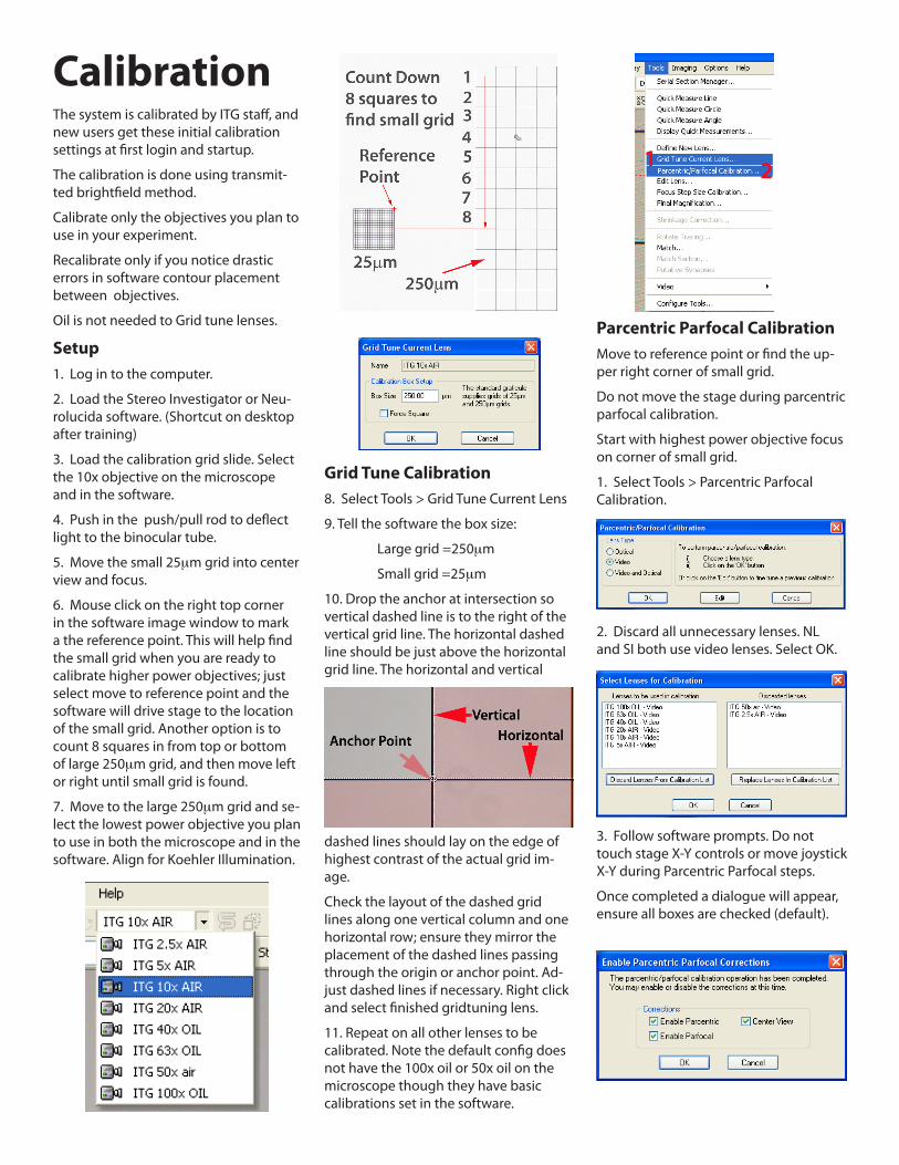
5. Move the small 25mm grid into center view and focus.

6. Mouse click on the right top corner in the software image window to mark a the reference point. This will help find the small grid when you are ready to calibrate higher power objectives; just select move to reference point and the software will drive stage to the location of the small grid. Another option is to count 8 squares in from top or bottom of large 250mm grid, and then move left or right until small grid is found.

7. Move to the large 250mm grid and se-lect the lowest power objective you plan to use in both the microscope and in the software. Align for Koehler Illumination.

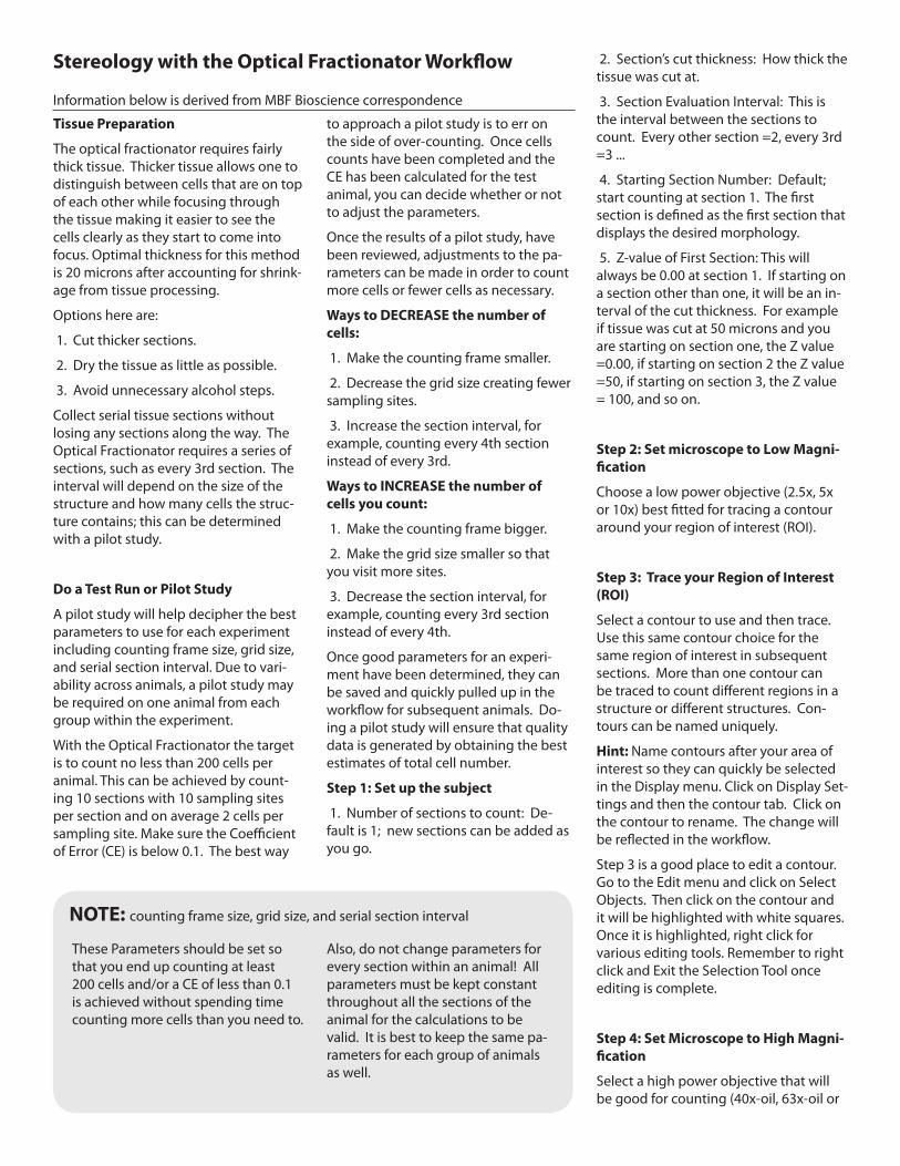
Grid Tune Calibration8. Select Tools > Grid Tune Current Lens

9. Tell the software the box size:

Large grid =250mm

Small grid =25mm

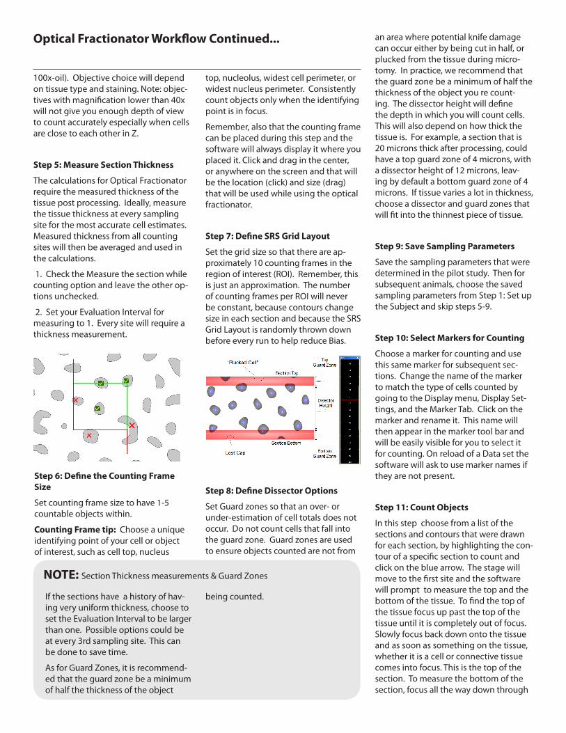
10. Drop the anchor at intersection so vertical dashed line is to the right of the vertical grid line. The horizontal dashed line should be just above the horizontal grid line. The horizontal and vertical

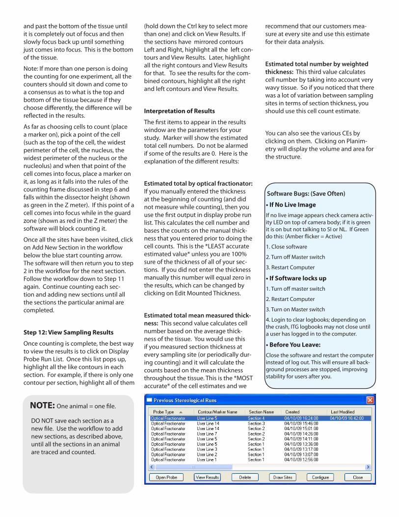
Parcentric Parfocal CalibrationMove to reference point or find the up-per right corner of small grid.

Do not move the stage during parcentric parfocal calibration.

Start with highest power objective focus on corner of small grid.

1. Select Tools > Parcentric Parfocal Calibration.

dashed lines should lay on the edge of highest contrast of the actual grid im-age.

Check the layout of the dashed grid lines along one vertical column and one horizontal row; ensure they mirror the placement of the dashed lines passing through the origin or anchor point. Ad-just dashed lines if necessary. Right click and select finished gridtuning lens.

11. Repeat on all other lenses to be calibrated. Note the default config does not have the 100x oil or 50x oil on the microscope though they have basic calibrations set in the software.

2. Discard all unnecessary lenses. NL and SI both use video lenses. Select OK.

3. Follow software prompts. Do not touch stage X-Y controls or move joystick X-Y during Parcentric Parfocal steps.

Once completed a dialogue will appear, ensure all boxes are checked (default).

Stereology with the Optical Fractionator Workflow

Tissue Preparation

The optical fractionator requires fairly thick tissue. Thicker tissue allows one to distinguish between cells that are on top of each other while focusing through the tissue making it easier to see the cells clearly as they start to come into focus. Optimal thickness for this method is 20 microns after accounting for shrink-age from tissue processing.

Options here are:

1. Cut thicker sections.

2. Dry the tissue as little as possible.

3. Avoid unnecessary alcohol steps.

Collect serial tissue sections without losing any sections along the way. The Optical Fractionator requires a series of sections, such as every 3rd section. The interval will depend on the size of the structure and how many cells the struc-ture contains; this can be determined with a pilot study.

Do a Test Run or Pilot Study

A pilot study will help decipher the best parameters to use for each experiment including counting frame size, grid size, and serial section interval. Due to vari-ability across animals, a pilot study may be required on one animal from each group within the experiment.

With the Optical Fractionator the target is to count no less than 200 cells per animal. This can be achieved by count-ing 10 sections with 10 sampling sites per section and on average 2 cells per sampling site. Make sure the Coefficient of Error (CE) is below 0.1. The best way

to approach a pilot study is to err on the side of over-counting. Once cells counts have been completed and the CE has been calculated for the test animal, you can decide whether or not to adjust the parameters.

Once the results of a pilot study, have been reviewed, adjustments to the pa-rameters can be made in order to count more cells or fewer cells as necessary.

Ways to DECREASE the number of cells:

1. Make the counting frame smaller.

2. Decrease the grid size creating fewer sampling sites.

3. Increase the section interval, for example, counting every 4th section instead of every 3rd.

Ways to INCREASE the number of cells you count:

1. Make the counting frame bigger.

2. Make the grid size smaller so that you visit more sites.

3. Decrease the section interval, for example, counting every 3rd section instead of every 4th.

Once good parameters for an experi-ment have been determined, they can be saved and quickly pulled up in the workflow for subsequent animals. Do-ing a pilot study will ensure that quality data is generated by obtaining the best estimates of total cell number.

Step 1: Set up the subject

1. Number of sections to count: De-fault is 1; new sections can be added as you go.

2. Section’s cut thickness: How thick the tissue was cut at.

3. Section Evaluation Interval: This is the interval between the sections to count. Every other section =2, every 3rd =3 ...

4. Starting Section Number: Default; start counting at section 1. The first section is defined as the first section that displays the desired morphology.

5. Z-value of First Section: This will always be 0.00 at section 1. If starting on a section other than one, it will be an in-terval of the cut thickness. For example if tissue was cut at 50 microns and you are starting on section one, the Z value =0.00, if starting on section 2 the Z value =50, if starting on section 3, the Z value = 100, and so on.

Step 2: Set microscope to Low Magni-fication

Choose a low power objective (2.5x, 5x or 10x) best fitted for tracing a contour around your region of interest (ROI).

Step 3: Trace your Region of Interest (ROI)

Select a contour to use and then trace. Use this same contour choice for the same region of interest in subsequent sections. More than one contour can be traced to count different regions in a structure or different structures. Con-tours can be named uniquely.

Hint: Name contours after your area of interest so they can quickly be selected in the Display menu. Click on Display Set-tings and then the contour tab. Click on the contour to rename. The change will be reflected in the workflow.

Step 3 is a good place to edit a contour. Go to the Edit menu and click on Select Objects. Then click on the contour and it will be highlighted with white squares. Once it is highlighted, right click for various editing tools. Remember to right click and Exit the Selection Tool once editing is complete.

Step 4: Set Microscope to High Magni-fication

Select a high power objective that will be good for counting (40x-oil, 63x-oil or

These Parameters should be set so that you end up counting at least 200 cells and/or a CE of less than 0.1 is achieved without spending time counting more cells than you need to.

Also, do not change parameters for every section within an animal! All parameters must be kept constant throughout all the sections of the animal for the calculations to be valid. It is best to keep the same pa-rameters for each group of animals as well.

NOTE: counting frame size, grid size, and serial section interval

Information below is derived from MBF Bioscience correspondence

Optical Fractionator Workflow Continued...

100x-oil). Objective choice will depend on tissue type and staining. Note: objec-tives with magnification lower than 40x will not give you enough depth of view to count accurately especially when cells are close to each other in Z.

Step 5: Measure Section Thickness

The calculations for Optical Fractionator require the measured thickness of the tissue post processing. Ideally, measure the tissue thickness at every sampling site for the most accurate cell estimates. Measured thickness from all counting sites will then be averaged and used in the calculations.

1. Check the Measure the section while counting option and leave the other op-tions unchecked.

2. Set your Evaluation Interval for measuring to 1. Every site will require a thickness measurement.

Step 6: Define the Counting Frame Size

Set counting frame size to have 1-5 countable objects within.

Counting Frame tip: Choose a unique identifying point of your cell or object of interest, such as cell top, nucleus

top, nucleolus, widest cell perimeter, or widest nucleus perimeter. Consistently count objects only when the identifying point is in focus.

Remember, also that the counting frame can be placed during this step and the software will always display it where you placed it. Click and drag in the center, or anywhere on the screen and that will be the location (click) and size (drag) that will be used while using the optical fractionator.

Step 7: Define SRS Grid Layout

Set the grid size so that there are ap-proximately 10 counting frames in the region of interest (ROI). Remember, this is just an approximation. The number of counting frames per ROI will never be constant, because contours change size in each section and because the SRS Grid Layout is randomly thrown down before every run to help reduce Bias.

If the sections have a history of hav-ing very uniform thickness, choose to set the Evaluation Interval to be larger than one. Possible options could be at every 3rd sampling site. This can be done to save time.

As for Guard Zones, it is recommend-ed that the guard zone be a minimum of half the thickness of the object

being counted.

NOTE: Section Thickness measurements & Guard Zones

Step 8: Define Dissector Options

Set Guard zones so that an over- or under-estimation of cell totals does not occur. Do not count cells that fall into the guard zone. Guard zones are used to ensure objects counted are not from

an area where potential knife damage can occur either by being cut in half, or plucked from the tissue during micro-tomy. In practice, we recommend that the guard zone be a minimum of half the thickness of the object you re count-ing. The dissector height will define the depth in which you will count cells. This will also depend on how thick the tissue is. For example, a section that is 20 microns thick after processing, could have a top guard zone of 4 microns, with a dissector height of 12 microns, leav-ing by default a bottom guard zone of 4 microns. If tissue varies a lot in thickness, choose a dissector and guard zones that will fit into the thinnest piece of tissue.

Step 9: Save Sampling Parameters

Save the sampling parameters that were determined in the pilot study. Then for subsequent animals, choose the saved sampling parameters from Step 1: Set up the Subject and skip steps 5-9.

Step 10: Select Markers for Counting

Choose a marker for counting and use this same marker for subsequent sec-tions. Change the name of the marker to match the type of cells counted by going to the Display menu, Display Set-tings, and the Marker Tab. Click on the marker and rename it. This name will then appear in the marker tool bar and will be easily visible for you to select it for counting. On reload of a Data set the software will ask to use marker names if they are not present.

Step 11: Count Objects

In this step choose from a list of the sections and contours that were drawn for each section, by highlighting the con-tour of a specific section to count and click on the blue arrow. The stage will move to the first site and the software will prompt to measure the top and the bottom of the tissue. To find the top of the tissue focus up past the top of the tissue until it is completely out of focus. Slowly focus back down onto the tissue and as soon as something on the tissue, whether it is a cell or connective tissue comes into focus. This is the top of the section. To measure the bottom of the section, focus all the way down through

DO NOT save each section as a new file. Use the workflow to add new sections, as described above, until all the sections in an animal are traced and counted.

NOTE: One animal = one file.

and past the bottom of the tissue until it is completely out of focus and then slowly focus back up until something just comes into focus. This is the bottom of the tissue.

Note: If more than one person is doing the counting for one experiment, all the counters should sit down and come to a consensus as to what is the top and bottom of the tissue because if they choose differently, the difference will be reflected in the results.

As far as choosing cells to count (place a marker on), pick a point of the cell (such as the top of the cell, the widest perimeter of the cell, the nucleus, the widest perimeter of the nucleus or the nucleolus) and when that point of the cell comes into focus, place a marker on it, as long as it falls into the rules of the counting frame discussed in step 6 and falls within the dissector height (shown as green in the Z meter). If this point of a cell comes into focus while in the guard zone (shown as red in the Z meter) the software will block counting it.

Once all the sites have been visited, click on Add New Section in the workflow below the blue start counting arrow. The software will then return you to step 2 in the workflow for the next section. Follow the workflow down to Step 11 again. Continue counting each sec-tion and adding new sections until all the sections the particular animal are completed.

Step 12: View Sampling Results

Once counting is complete, the best way to view the results is to click on Display Probe Run List. Once this list pops up, highlight all the like contours in each section. For example, if there is only one contour per section, highlight all of them

(hold down the Ctrl key to select more than one) and click on View Results. If the sections have mirrored contours Left and Right, highlight all the left con-tours and View Results. Later, highlight all the right contours and View Results for that. To see the results for the com-bined contours, highlight all the right and left contours and View Results.

Interpretation of Results

The first items to appear in the results window are the parameters for your study. Marker will show the estimated total cell numbers. Do not be alarmed if some of the results are 0. Here is the explanation of the different results:

Estimated total by optical fractionator: If you manually entered the thickness at the beginning of counting (and did not measure while counting), then you use the first output in display probe run list. This calculates the cell number and bases the counts on the manual thick-ness that you entered prior to doing the cell counts. This is the *LEAST accurate estimated value* unless you are 100% sure of the thickness of all of your sec-tions. If you did not enter the thickness manually this number will equal zero in the results, which can be changed by clicking on Edit Mounted Thickness.

Estimated total mean measured thick-ness: This second value calculates cell number based on the average thick-ness of the tissue. You would use this if you measured section thickness at every sampling site (or periodically dur-ing counting) and it will calculate the counts based on the mean thickness throughout the tissue. This is the *MOST accurate* of the cell estimates and we

recommend that our customers mea-sure at every site and use this estimate for their data analysis.

Estimated total number by weighted thickness: This third value calculates cell number by taking into account very wavy tissue. So if you noticed that there was a lot of variation between sampling sites in terms of section thickness, you should use this cell count estimate.

You can also see the various CEs by clicking on them. Clicking on Planim-etry will display the volume and area for the structure.

Software Bugs: (Save Often)

• If No Live Image

If no live image appears check camera activ-ity LED on top of camera body; if it is green it is on but not talking to SI or NL. If Green do this: (Amber flicker = Active)

1. Close software

2. Turn off Master switch

3. Restart Computer

• If Software locks up

1. Turn off master switch

2. Restart Computer

3. Turn on Master switch

4. Login to clear logbooks; depending on the crash, ITG logbooks may not close until a user has logged in to the computer.

• Before You Leave:

Close the software and restart the computer instead of log out. This will ensure all back-ground processes are stopped, improving stability for users after you.

Start-up

1 . . . . . . . . . Turn ON Master Switch2 . . . . . . . . . . . Log on to Computer3 . . . . . . . . . . . . . Load SoftwareOptional . . . . .Turn ON X-Cite Hg Lamp

Align Optical Components 1 . . . . . . . . . . . Koehler Illumination

Calibrate System 1 . . . . . . . . . . . . . Grid Tune Lens2 . . . . . . Parcentric Parfocal Calibration

Run Experiment 1 . . . . . . . . . . . . . .Set up Subject2 . . . . . . . . . . Set scope to Low Mag3 . . . . . . . . Trace Region(s) of interest4 . . . . . . . . . .Set scope to High Mag5 . . . . . . . Define Counting Frame Size6 . . . . . . . . . Define SRS Grid Layout7 . . . . . . . . . Define Disector Options8 . . . . . . . . Save Sampling Paramters9 . . . . . . . Select Markers for Counting10 . . . . . . . . . . . . .Count Objects11 . . . . . . . . .View Sampling Results

Save Files . . . . . . . . . . . . . 1 . . . . .Save to local machine-(often)2 . . . . . . . Copy Files Server (Zeus)

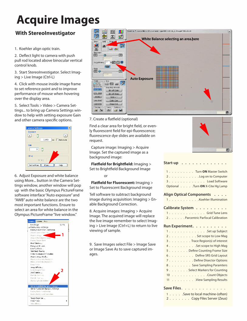
1. Koehler align optic train.

2. Deflect light to camera with push pull rod located above binocular vertical control knob.

3. Start StereoInvestigator. Select Imag-ing > Live Image (Ctrl-L)

4. Click with mouse inside image frame to set reference point and to improve performance of mouse when hovering over the display area.

5. Select Tools > Video > Camera Set-tings... to bring up Camera Settings win-dow to help with setting exposure Gain and other camera specific options.

6. Adjust Exposure and white balance using More... button in the Camera Set-tings window, another window will pop up with the basic Olympus PictureFrame software interface “Auto exposure” and “AWB” auto white balance are the two most important functions. Ensure to select an area for white balance in the Olympus PictureFrame “live window.”

With StereoInvestigator

Acquire Images

7. Create a flatfield (optional)

Find a clear area for bright field, or even-ly fluorescent field for epi-fluorescence; fluorescence dye slides are available on request.

Capture image: Imaging > Acquire Image. Set the captured image as a background image:

Flatfield for Brightfield: Imaging > Set to Brightfield Background Image

or

Flatfield for Fluorescent: Imaging > Set to Fluorescent Background image

Tell software to subtract background image during acquisition: Imaging > En-able Background Correction.

8. Acquire images: Imaging > Acquire Image. The acquired image will replace the live image remember to select Imag-ing > Live Image (Ctrl+L) to return to live viewing of sample.

9. Save Images select File > Image Save or Image Save As to save captured im-ages.

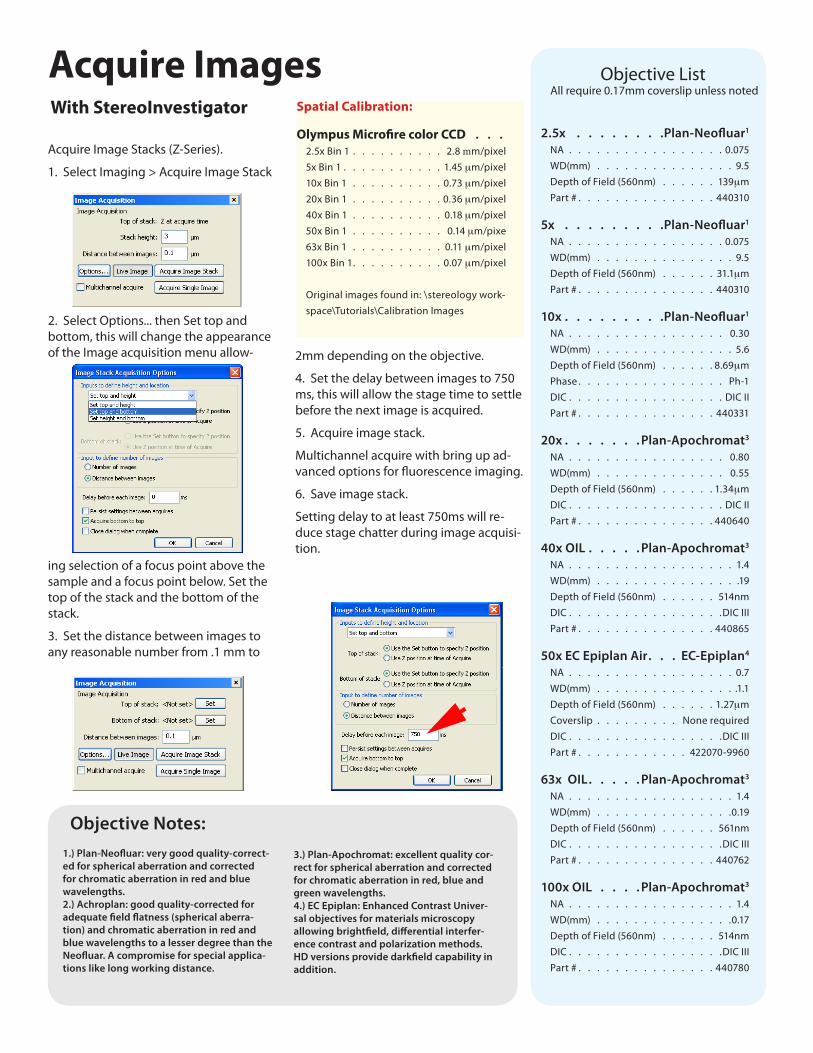
Acquire Images Objective List All require 0.17mm coverslip unless noted

2 5x Plan-Neofluar1

NA . . . . . . . . . . . . . . . . . 0.075WD(mm) . . . . . . . . . . . . . . . 9.5Depth of Field (560nm) . . . . . . 139mmPart # . . . . . . . . . . . . . . . 440310

5x Plan-Neofluar1

NA . . . . . . . . . . . . . . . . . 0.075WD(mm) . . . . . . . . . . . . . . . 9.5Depth of Field (560nm) . . . . . . 31.1mmPart # . . . . . . . . . . . . . . . 440310

10x Plan-Neofluar1

NA . . . . . . . . . . . . . . . . . 0.30WD(mm) . . . . . . . . . . . . . . . 5.6Depth of Field (560nm) . . . . . . 8.69mmPhase . . . . . . . . . . . . . . . . Ph-1DIC . . . . . . . . . . . . . . . . . DIC IIPart # . . . . . . . . . . . . . . . 440331

20x Plan-Apochromat3

NA . . . . . . . . . . . . . . . . . 0.80WD(mm) . . . . . . . . . . . . . . 0.55Depth of Field (560nm) . . . . . . 1.34mmDIC . . . . . . . . . . . . . . . . . DIC IIPart # . . . . . . . . . . . . . . . 440640

40x OIL Plan-Apochromat3

NA . . . . . . . . . . . . . . . . . . 1.4WD(mm) . . . . . . . . . . . . . . . .19Depth of Field (560nm) . . . . . . 514nmDIC . . . . . . . . . . . . . . . . .DIC IIIPart # . . . . . . . . . . . . . . . 440865

50x EC Epiplan Air EC-Epiplan4

NA . . . . . . . . . . . . . . . . . . 0.7WD(mm) . . . . . . . . . . . . . . . .1.1Depth of Field (560nm) . . . . . . 1.27mmCoverslip . . . . . . . . . None requiredDIC . . . . . . . . . . . . . . . . .DIC IIIPart # . . . . . . . . . . . . 422070-9960

63x OIL Plan-Apochromat3

NA . . . . . . . . . . . . . . . . . . 1.4WD(mm) . . . . . . . . . . . . . . .0.19Depth of Field (560nm) . . . . . . 561nmDIC . . . . . . . . . . . . . . . . .DIC IIIPart # . . . . . . . . . . . . . . . 440762

100x OIL Plan-Apochromat3

NA . . . . . . . . . . . . . . . . . . 1.4WD(mm) . . . . . . . . . . . . . . .0.17Depth of Field (560nm) . . . . . . 514nmDIC . . . . . . . . . . . . . . . . .DIC IIIPart # . . . . . . . . . . . . . . . 440780

Objective Notes:1 ) Plan-Neofluar: very good quality-correct-ed for spherical aberration and corrected for chromatic aberration in red and blue wavelengths 2 ) Achroplan: good quality-corrected for adequate field flatness (spherical aberra-tion) and chromatic aberration in red and blue wavelengths to a lesser degree than the Neofluar A compromise for special applica-tions like long working distance

3 ) Plan-Apochromat: excellent quality cor-rect for spherical aberration and corrected for chromatic aberration in red, blue and green wavelengths 4 ) EC Epiplan: Enhanced Contrast Univer-sal objectives for materials microscopy allowing brightfield, differential interfer-ence contrast and polarization methods HD versions provide darkfield capability in addition

Acquire Image Stacks (Z-Series).

1. Select Imaging > Acquire Image Stack

Spatial Calibration:

Olympus Microfire color CCD 2.5x Bin 1 . . . . . . . . . . 2.8 mm/pixel5x Bin 1 . . . . . . . . . . . 1.45 mm/pixel10x Bin 1 . . . . . . . . . . 0.73 mm/pixel20x Bin 1 . . . . . . . . . . 0.36 mm/pixel40x Bin 1 . . . . . . . . . . 0.18 mm/pixel50x Bin 1 . . . . . . . . . . 0.14 mm/pixe63x Bin 1 . . . . . . . . . . 0.11 mm/pixel100x Bin 1 . . . . . . . . . . 0.07 mm/pixel

Original images found in: \stereology work-space\Tutorials\Calibration Images

2. Select Options... then Set top and bottom, this will change the appearance of the Image acquisition menu allow-

ing selection of a focus point above the sample and a focus point below. Set the top of the stack and the bottom of the stack.

3. Set the distance between images to any reasonable number from .1 mm to

With StereoInvestigator

2mm depending on the objective.

4. Set the delay between images to 750 ms, this will allow the stage time to settle before the next image is acquired.

5. Acquire image stack.

Multichannel acquire with bring up ad-vanced options for fluorescence imaging.

6. Save image stack.

Setting delay to at least 750ms will re-duce stage chatter during image acquisi-tion.

Saving files

1. Save to Local Machine. --Default

You may save files to Workspace (E:\Workspace\”username”). A folder was created there at login for each user.

2. Before leaving, save to Network Share -- “username” on ‘ITG File Server (zeus.itg.uiuc.edu)’(Z:)

Most users opt to save the data to their network share on our central server (named Zeus). The server share is represented as the ‘Z:\’ drive in the windows environment. ITG is equipped with gigabit ethernet, and saving to the Z:\ drive is relatively fast. Also, this permits easy access to the data from any computer in the world using secure file transfer protocol (sftp). Instructions on accessing your network share remotely are available at http://www.itg.uiuc.edu/help/datahandling/userhelp.htm.

Saving as TIFFs (.tif )

Single images, z-stacks, multi-channel images will be saved as a series of TIFF images that can be viewed in other programs (Adobe Photoshop, ImageJ, Imaris, Image Pro Plus etc…).

ReferencesCalibration Standards

Calibration Grid Slide from Micro Brightfield:

http://www.mbfbioscience.com

Fluorescent Reference Slides from Micros-copy Education:

http://www.microscopyeducation.com

Olympus

http://www.olympusamerica.com/seg_sec-tion/seg_home.asp

--Olympus Microfire color CCD• CCD Array: 1600 x 1200 Pixels

• CCD Size: 14.8 mm diagonal

• Pixel Size: 7.4 microns square

• Architecture: Interline CCD, Progressive scan (noninterlaced)

• Well Depth: 40,000 electrons

• Read Noise: 20 electrons rms

• Dark Current: 0.3 nA/cm2

• Dynamic Range: 60 dB

• Exposure Time Range: 500 microseconds - 60 seconds

• Gain Range: 1x - 16x

• Bit Depth: 12-bit Monochrome

Commercial anti-fade mounting media

• ProLong Gold Antifade Mountant:

http://www.invitrogen.co.jp/products/pdf/mp36930.pdf

• Vectashield Antifade Mounting Medium:

http://www.vectorlabs.com/VECTASHIELD/ VECTASHIELD.html

• VECTASHIELD HardSet Mounting Medium:

http://www.vectorlabs.com/products.details.asp?prodID=1483

Fluorescence Microscopy Books/Papers

Allan, V., Ed., Protein Localization by Fluo-rescence Microscopy: A Practical Approach, Oxford University Press (1999).

Andreeff, M. and Pinkel, D., Eds., Introduction to Fluorescence In Situ Hybridization: Prin-ciples and Clinical Applications, John Wiley and Sons (1999).

Herman, B., Fluorescence Microscopy, Second Edition, BIOS Scientific Publishers (1998).

Michalet, X., Kapanidis, A.N., Laurence, T., Pinaud, F., Doose, S., Pflughoefft, M. and Weiss S., “The power and prospects of

fluorescence microscopies and spectrosco-pies,” Annu Rev Biophys Biomolec Struct 32, 161–182 (2003).

Murphy, D.B., Fundamentals of Light Micros-copy and Electronic Imaging, John Wiley and Sons (2001). Molecular Probes.

Spector, D.L. and Goldman, R.D., Basic Methods in Microscopy, Cold Spring Harbor Laboratory Press (2005).

Yuste, R. and Konnerth, A., Eds., Imaging in Neuroscience and Development: A Labora-tory Manual, Cold Spring Harbor Laboratory Press (2004).

Stereology References

Online Assistance:

http://www.mbfbioscience.com/live-support/

FAQ:

http://www.mbfbioscience.com/faqs/

Stereology References:

http://www.mbfbioscience.com/stereo-investigator-bibliography/

Chroma Filter Sets for AxioImager A1

Excitation Wheel

(1) Blank(2) Dual Cy2/Cy3(3) 350/50(4) 402/15(5) 490/20(6) 555/25(7) 645/30(8) Blank-blocked(9) Blank-blocked(10) Blank-blocked

Emission Wheel by Camera

(1) IR filter(2) Dual Cy2/Cy3(3) 455/50(4) 525/36(5) 605/52(6) 705/72(7) Blank-blocked(8) Blank-blocked(9) Blank-blocked(10) Blank no IR filter

Filter Cubes/Dichroics

(1) Transmitted cube with polarizer(2) Cy2/Cy3 filter cube for viewing through binoculars(3) 3channel Dichroic --Camera only(4) 4 channel Dichroic --Camera only(5) Blank(6) Reflected Brightfield cube

Imaging Technology Group

Beckman Institute for Advanced Science and Technology

University of Illinois at Urbana-Champaign

405 North Mathews, Urbana IL 61801 USA

Phone: 217.244.0170 FAX: 217.244.6219