The relaxed investor and parameter uncertaintysgerhold/pub_files/sem12/... · 2012-03-02 · One feature of this solution is that the agent trying to implement it will be continuously

Finance Stochast. 5, 131–154 (2001)

c© Springer-Verlag 2001

The relaxed investor and parameter uncertainty

L.C.G. Rogers

University of Bath, Department of Mathematical Sciences, Bath BA2 7AY, UK(e-mail: [email protected])

Abstract. We firstly consider an investor faced with the classical Merton problemof optimal investment in a log-Brownian asset and a fixed-interest bond, butconstrained only to change portfolio (and, if relevant, consumption) choices attimes which are a multiple ofh. We show that the cost of this constraint can bewell described by a power series expansion inh, the first few terms of which wedetermine explicitly. Typically, this cost is not too large. We then compare thiswith the cost of parameter uncertainty, as modelled by supposing that the rateof return on the share has a prior Gaussian distribution. We find that the effectof parameter uncertainty is typically bigger than the effects of infrequent policyreview.

Key words: Merton consumption problem, Merton investment problem, timelag, parameter uncertainty

JEL Classification: C61, D81, D90, G11

AMS (1991) Subject Classification: 90A09, 90A10, 90A43

1 Introduction

In the classical Merton investment/consumption model (Merton (1969)), an agentwho may invest in a log-Brownian share1 and a constant interest rate moneymarket account seeks to maximise the expected integrated utility of consumption,subject to the constraint that wealth remains non-negative at all times. For the case

Supported partly by EPSRC grants GR/J97281 and GR/L10000.1 We consider only a single share throughout this paper; multiple shares can be handled similarly,with slightly more tiresome notation.

Manuscript received: November 1999; final version received: June 2000

132 L.C.G. Rogers

where the utility is constant relative risk aversion (that is,U (c) = c1−R/(1 − R)for someR > 0), Merton finds that the optimal behaviour of the agent is alwaysto invest a fixed proportion of wealth in the risky asset, and always to consumeat a rate proportional to wealth. The constants of proportionality have explicitexpressions in terms of the parameters of the problem2.

One feature of this solution is that the agent trying to implement it willbe continuously adjusting the share holding and the consumption rate, which isclearly impractical. A more realistic scenario would be that the agent chooses toreview his investment and consumption decisions on a regular basis, at intervalsof some fixed positiveh; think of the agent as lazy (or relaxed!) if you wish, orperhaps as having other things to do with his life. Alternatively, the agent maybe reluctant to rebalance often due to the presence of transactions costs, and wecan consider this study as an attempt to decouple the two effects which act in atransactions-costs problem; the losses due to imperfect portfolio balance inducedby infrequent portfolio revision, and the losses due to transactions costs. We shallhave more to say on this in the conclusions section.

For brevity, we call an agent constrained in this way anh-investor. Theclass of investment/consumption policies available to theh-investor is a subsetof those available to the Merton investor, so his objective will be smaller thanthat of the Merton investor - but by how much? It appears to be impossible toanswer this question in closed form, but by deriving a series expansion in the(small) parameterh, we shall find remarkably good approximations which allowus to conclude that the cost of a relaxed approach is surprisingly small, at least ifthe Merton proportion is in [0, 1]. At first sight, we might expect that the Mertonsolution should be the limit ash ↓ 0 of the solution for theh-investor, but thisturns out to be true only if the Merton proportion is in [0, 1]; the h-investor willnever borrow to buy the share, nor sell the share short, because in a time intervalof length h the share price could move disastrously, and the investor would bewiped out. The Merton investor on the other hand would simply adjust his holdingof the share as the price moved and would keep his wealth non-negative. Thusif the Merton proportion is not in [0,1], there is a difference between the Mertoninvestor and the 0+-investor, and this is the main effect. It is worth remarkingthat situations where the Merton proportion is not in [0,1] are not common inpractice.

The h-investor’s problem reduces to a problem in discrete time, the formof whose solution is known from the work of Hakansson (1970); nevertheless,this solution is less explicit than the solution of Merton, in that it involves thesolution of a one-step optimisation problem which cannot be found in closedform. In this paper, we take the view that the parameterh is small, and we finda series expansion for the optimal solution. It turns out that the first three termsof this expansion are already enough for the selection of situations we took fornumerical examples.

2 Merton solves the problem by solving the associated HJB equation. This technique is restrictedin its scope, but the problem can be solved in much greater generality; see, for example, Karatzas(1989)

The relaxed investor 133

The paper is organised as follows. In Sect. 2, we briefly review the two clas-sical Merton problems, the wealth problem (where the agent’s objective is tomaximise the expected utility of wealth at some fixed terminal time), and theconsumption problem (where the objective is to maximise the expected integratedutility of consumption over all future time). Then in Sect. 3 we investigate theimpact of the lag on the wealth problem, and find a power-series expansion inpowers ofh for the loss of efficiency, as well as the optimal investment policy.3 In Sect. 4, we perform the corresponding analysis for the Merton consumptionproblem. In both cases, we check our results against exact numerically computedanswers, and find that the power series is very accurate, and also that the magni-tude of the effect is small. Section 5 discusses why this should be a small effect;the main reason is that the payoff of a fixed-proportion rule is quite insensitive tothe chosen proportion in a neighbourhood of the Merton proportion. However, theneighbourhood where the payoff is affected little is actually quitesmall comparedto the confidence interval for the rate-of-return parameter which one would getfrom a typical length of data; so this leads us in Sects. 6 and 7 to investigate theeffect of uncertainty in the rate-of-return parameter. We assume that this param-eter has a Gaussian prior distribution, and then use techniques of filtering theoryto derive the optimal rules. The use of such techniques in financial economicsis far from new; Bawa et al. (1979), Klein and Bawa (1976), Klein and Bawa(1977), Dothan and Feldman (1986), Feldman (1989), Gennotte (1986), Lakner(1995), Browne and Whitt (1996), Lakner (1998), Karatzas and Zhao (1998),Brennan (1998) is a selection of references dealing with classical economic op-timisation problems complicated by a Bayesian updating of unknown parameterdistributions. Browne and Whitt (1996) solve the Merton wealth problem in thecase of logarithmic utility, and Lakner (1995) deals with general utility.

Finally, in Sect. 8 we conclude, and discuss the relationship between ourresults and earlier results on transactions costs.

2 The classical Merton wealth and consumption problems

An investor may invest in two assets, a money market account with constantinterest rater , and a share with price process (St )t≥0 satisfying

dSt = St (σdWt + αdt) (2.1)

for constantsσ andα, where (Wt )t≥0 is a standard Brownian motion.In the Merton wealth problem, the investor chooses to holdθt in the share at

time t , so that his wealth evolves as

dwt = rwt dt + θt (σdWt + (α − r)dt), (2.2)

and he aims to maximise his objective

3 There is a growing literature on approximate hedging under finite rebalancing restrictions; see,for example, the preprint of Martini and Patry (2000) and the references therein.

134 L.C.G. Rogers

E U (wT ), (2.3)

whereT > 0 is some fixed time horizon, and the utilityU is constant relativerisk aversion (CRRA):

U (c) =c1−R

1 − R(2.4)

for some positiveR, (R /= 1).4 The optimal behaviour is to invest a fixed multipleof wealth in the risky asset at all times:θt = πwt for some constantπ. A fewlines of calculations shows that if the agent does indeed follow the ruleθt = πwt ,then the value of his objective is

U (w0) exp

[(1 − R)T

{π(α − r) + r − 1

2Rπ2σ2

}], (2.5)

which is optimised by takingπ = π∗, where

π∗ =α − rσ2R

(2.6)

is the so-calledMerton proportion, though we note that in general it does notneed to lie in [0, 1]. The optimised value is

U (w0) exp

((1 − R)T

(r +

12σ2Rπ2

∗

)). (2.7)

In the Merton consumption problem, the investor chooses to holdθt in theshare at timet and to consume at ratect at time t , so that his wealth at timet ,wt , evolves according to the wealth equation

dwt = (rwt − ct )dt + θt (σdWt + (α − r)dt). (2.8)

Subject to the constraint thatwt ≥ 0 for all t , his objective is to maximise

E∫ ∞

0e−ρt U (ct )dt (2.9)

where ρ > 0 is constant, and the utilityU is as at (2.4) Denoting the valuefunction for this problem byVM , Merton [5] finds the following explicit formfor the solution:

VM (w) = γ−R∗ U (w), (2.10)

θt = π∗wt , (2.11)

ct = γ∗wt , (2.12)

whereπ∗ is the Merton proportion (2.6), and

4 The case ofR = 1 corresponds to logarithmic utility and needs to be treated separately, but theresults remain very similar; the details of this case are left to the interested reader.

The relaxed investor 135

γ∗ =ρ + (R − 1)(r + (α − r)2/2Rσ2)

R(2.13)

=ρ + (R − 1)(r + 1

2σ2Rπ2∗)

R. (2.14)

There is no need to repeat Merton’s proof here. In view of the scale-invariantnature of the problem, the form of the solution is not perhaps surprising; underthe assumption that the investor is going to choose to holdθt = πwt and consumeat rateγwt for some constantsπ andγ, the wealth of the investor is easily seento be

wt = w0 exp(πσWt + (r − γ + π(α − r) − π2σ2/2)t)

and his payoff is easily computed to be

E∫ ∞

0e−ρt U (γwt )dt =

(γw0)1−R

1 − R

[ρ+(R−1)(r −γ+π(α−r)−Rπ2σ2/2)

]−1.

(2.15)Once again, a little calculus shows that the optimal choices ofπ and γ are asstated.

3 The h-investor’s wealth problem

Suppose we take the Merton wealth problem for theh-investor with a fixedtime horizon T = Nh; the investor is only going to change his portfolio attimes which are multiples ofh and aims to maximise the objective (2.3). Hisproblem is a discrete-time dynamic programming problem, whose value functionVn (w) ≡ supE [U (wT )|wnh = w] has the form

Vn (w) = AN −nU (w), (3.1)

where

A = (1− R) supp∈[0,1]

E(pZ + (1− p)erh )1−R

1 − R≡ (1 − R)κ. (3.2)

Here,Z ≡ exp(σWh + (α − σ2/2)h) is the random return on the risky asset in atime interval of lengthh. Notice thatA is positive whatever the value ofR.

Proof of (3.1) The Bellman equation linksVn andVn+1 by

Vn (w) = supp∈[0,1]

E Vn+1(pwZ + (1− p)werh ); (3.3)

the agent chooses the proportionp of his wealth to invest in the risky asset (andthis proportion must be in [0, 1] as discussed in the introduction), and aims tomaximise the expected derived utility of wealth at the next time point. We knowthat VN = U , and so by induction if (3.1) holds for alln > m, we have from(3.3)

136 L.C.G. Rogers

Vm (w) = supp∈[0,1]

E AN −m−1U (pwZ + (1− p)werh )

= AN −m−1w1−R supp∈[0,1]

E(pZ + (1− p)erh )1−R

1 − R

= U (w)AN −m

as required. ��

We therefore have an expressionAN U (w0) for the optimal value of the objec-tive of theh-investor which we can compare with the value (2.6) of the Mertoninvestor. But how should we compare the two? The natural measure is theeffi-ciency.

Definition 1 The efficiencyΘ(h) of the h-investor relative to the Merton investoris the amount of wealth at time 0 which the Merton investor would need to obtainthe same maximised expected utility at time h as the h-investor who started attime 0 with unit wealth:

Θ(h) = A1/(1−R) exp

(−h

(r +

12σ2Rπ2

∗

)). (3.4)

It appears that there is no simple closed-form expression for the efficiency for thisproblem, but as we shall see it is perfectly possible to derive a good expansionfor Θ in powers ofh. The only part of the expression (3.4) for the efficiencywhich is mysterious is

κ ≡ supp∈[0,1]

E(pZ + (1− p)erh )1−R

1 − R,

which we aim to explain. Thinking ofh as a small parameter, the two termsZ and erh in the expression forκ are both close to 1, so we make a binomialexpansion of (pZ + (1− p)erh )1−R . Defining

X ≡ p(Z − 1) + (1− p)(erh − 1)

= p(exp(σWh + (α − σ2/2)h) − 1) + (1− p)(erh − 1),

we have for anyN ≥ 0

E(1 + X )1−R

1 − R= E

[1

1 − R

2N∑j=0

Γ (2 − R)Γ (2 − R − j )

X j

j !

+1

1 − RΓ (2 − R)

Γ (2 − R − 2N − 1)(1 + θX )−R−2N X 2N +1

(2N + 1)!

],

(3.5)

where the random variableθ takes values in [0, 1]. In order to control the re-mainder term, we need the estimation provided by the following result.

The relaxed investor 137

Proposition 1 For each N ∈ Z+, there exists CN = CN (R, σ, α, r) such that for

every 0 ≤ h ≤ 1, for any random variable θ with values in [0, 1], and for anyp ∈ [0, 1] we have

E |(1 + θX )−R−2N X 2N +1| ≤ CN h (2N +1)/2.

Proof. See Appendix. ��

Hence the Taylor expansion (3.5) reduces to the statement

E(1 + X )1−R

1 − R=

11 − R

2N∑j=0

Γ (2 − R)Γ (2 − R − j )

EX j

j !+ O(h (2N +1)/2), (3.6)

and all of the expectations appearing in this expression can be evaluated in closedform, sinceX is raised to an integer power.

Whenπ∗ ∈ (0, 1), the optimal choice forp to pick the point of [0, 1] nearestto π∗, and this is covered in Theorems 1 and 3 below. The interesting case iswhen π∗ ∈ (0, 1), Theorem 2, when we express the optimalp as an analyticfunction5 of h, p(h) =

∑n≥0 pn hn , and to use (3.6) to obtain as many terms

in the expansion as are required. The calculations were done using Maple, andwe present below the expansion ofp up to terms inh of order 2, as well asthe corresponding expansion of the optimal consumption rate, and the efficiency.There are three cases to be considered, according as the Merton proportionπ∗ isless than 0, in [0,1], or greater than 1, and we present the three cases separately.

Theorem 1 In the case π∗ ≤ 0, the optimal choice of p is 0. The efficiency is

Θ(h) = exp

(−1

2Rhσ2π2

∗

). (3.7)

Theorem 2 In the case 0 < π∗ < 1, the expansion Θ(h) =∑

n≥0 Θnhn , of theefficiency is given up to order 3 by

Θ0 = 1 (3.8)

Θ1 = 0 (3.9)

Θ2 = −14

Rπ2∗σ

4(1 − π∗)2 (3.10)

Θ3 = −Rπ2∗σ

6(1 − π∗)2(4Rπ2∗ − 4Rπ∗ − 1)/24 (3.11)

The optimal proportion has a power series expansion the first three terms of whichare

5 The analyticity of the optimalp as a function ofh follows from the analyticity ofκ in aneighbourhhod ofp = π∗, h = 0, by the Implicit Function Theorem.

138 L.C.G. Rogers

p0 = π∗ (3.12)

p1 = σ2π∗

(π∗ − 1

2

)(1 − π∗) (3.13)

p2 = −σ4π∗(2π∗ − 1)(π∗ − 1)(6Rπ2∗ − 6Rπ∗ − 1)/12 (3.14)

Theorem 3 In the case π∗ ≥ 1, the optimal choice of p is 1. The efficiency is

Θ(h) = exp

(−1

2Rhσ2(1 − π∗)2

). (3.15)

In the situation of Theorem 1, the optimal choice ofp is 0, and so from (3.2)we find thatA = erh , and the stated expression (3.7) for the efficiency followsfrom the definition (3.4).

Similarly, in the situation of Theorem 1, the optimal choice ofp is 1, and sofrom (3.2) we find thatA = exp(αh − σ2Rh/2); substituting into the definition(3.4) of the efficiency yields (3.15), using the definition (2.6) ofπ∗.

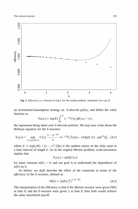
The expansion reported in Theorem 2 was obtained using Maple. As a check,we computed the exact values ofκ for the lagsh = 2−i/2, i = −4, . . . , 6 andcompared them with the asymptotics of Theorem 2. The parameter values usedwere σ = 0.35, r = 0.1, α = 0.18 andR = 4, resulting in the value 0.1632653for π∗, and Fig. 1 displays a graph of the numerically-computed values (markedas dots) together with the asymptotic values, computed from the power seriesexpansion up to terms inh5.

We see that the asymptotic is very accurate out to lags of 2 years, whichwould be a long time for most investors to leave their portfolio unchanged. Wealso see that the numerical values of the efficiency arevery close to unity; evenfor a 4-year lag, the loss of efficiency is only 0.36 %.

In Theorem 2 we find that the loss of efficiency isO(h2). What we typicallyhave in mind is that the investor has a time horizonT > 0 and will reviewthe portfolio N times before the time horizon, at intervals of lengthh = T/N .Thus if we compare the performance over [0, T ] of the Merton investor andthe h-investor, we shall find that the efficiency of theh-investor isΘ(h)N , andtherefore to leading order the loss of efficiency is1

4Rπ2∗σ

4(1−π∗)2Th. This O(h)loss of efficiency is seen also in the effect on the Merton consumption problem.

4 The h-investor’s consumption problem

In this section, we turn to the consumption problem of Merton.Theh-investormakes a sequence of decisions at the timesnh, n ∈ Z. Specifically, at timenh he sets aside an amountch of wealth to be consumed at ratec during theinterval [nh, nh + h), and then chooses a proportionp ≡ 1 − q of his remainingwealth w − ch to be invested in the risky asset until the next decision timenh + h. Of course, all of the decisions have to be non-anticipating. We call such

The relaxed investor 139

••

•••••••••••••••••••

h

effic

ienc

y

0 1 2 3 4

0.99

00.

995

1.00

01.

005

1.01

0

Fig. 1. Efficiency as a function of lagh for the wealth problem. Parameters for case B

an investment/consumption strategy anh-discrete policy, and define the valuefunction as

Vh (w) ≡ supE [∫ ∞

0e−ρt U (ct )dt |w0 = w],

the supremum being taken overh-discrete policies. We may now write down theBellman equation for theh-investor:

Vh (w) = supc≥0,p∈[0,1]

U (c)1 − e−ρh

ρ+e−ρhE

[Vh ((w−ch)(pZ +(1−p)erh ))

], (4.1)

whereZ ≡ exp(σWh + (α − σ2/2)h) is the random return on the risky asset ina time interval of lengthh. As in the original Merton problem, scale-invarianceimplies that

Vh (w) = a(h)U (w)

for some constanta(h) > 0, and our goal is to understand the dependence ofa(h) on h.

As before, we shall describe the effect of the constraint in terms of theefficiency of the h-investor, defined as

Θ(h) ≡ (a(h)γR

∗)1/(1−R)

. (4.2)

The interpretation of the efficiency is that if the Merton investor were givenΘ(h)at time 0, and theh-investor were given 1 at time 0, then both would achievethe same maximised payoff.

140 L.C.G. Rogers

Using the scaling ofVh , the Bellman equation for the problem becomes

a(h)1 − R

= supγ≥0,p∈[0,1]

hγ1−R

1 − R+ a(h)e−ρh (1 − γh)1−RE

(pZ + (1− p)erh )1−R

1 − R,

(4.3)whereh = (1− e−ρh )/ρ. Inspection of (4.3) reveals a decoupling of the maximi-sation problem; indeed, if we take as before

κ ≡ supp∈[0,1]

E(pZ + qerh )1−R

1 − R, (4.4)

then the Bellman equation (4.3) can be expressed more simply as

a(h)1 − R

= supγ≥0

[h

γ1−R

1 − R+ a(h)e−ρh (1 − γh)1−Rκ

],

and this can be maximised explicitly overγ. We find that

a(h)1/R =h(h/h)1/R

1 − (κ(1 − R)e−ρh )1/R, (4.5)

γ = h−1

[1 − (κe−ρh (1 − R))1/R

](4.6)

≡ γ(h). (4.7)

Now we saw in the previous section how to deal withκ, by supposing that theoptimal proportion has an analytic expansion in powers ofh, and computingthe leading terms in that expansion. Once again, there are three cases to beconsidered, according as the Merton proportionπ∗ is less than 0, in [0,1], orgreater than 1, and we present them separately.

Theorem 4 In the case π∗ ≤ 0, the optimal choice of p is 0, and the optimal κis exp(r(1− R)h)/(1− R). Using (4.2), (4.4), (4.5), and (4.6), the efficiency Θ(h)and consumption rate γ(h) have explicit expressions, with expansions Θ(h) =∑

n≥0 Θnhn and γ(h) =∑

n≥0 γnhn given up to order 2 by

Θ0 =

[1 +

(σπ∗)2R(R − 1)2(ρ + (R − 1)r)

]R/(1−R)

(4.8)

Θ1 = −rΘ0/2 (4.9)

Θ2 =4r2R − (r − ρ)2

24RΘ0 (4.10)

and

γ0 =ρ + (R − 1)r

R(4.11)

γ1 = −γ20

2(4.12)

γ2 =γ3

0

6(4.13)

The relaxed investor 141

Theorem 5 In the case 0 < π∗ < 1, the expansions Θ(h) =∑

n≥0 Θnhn , andγ(h) =

∑n≥0 γnhn of the efficiency up to order 2, and the consumption rate up

to order 1 are given by

Θ0 = 1 (4.14)

Θ1 = −12

r − 14π2

∗σ2R − π2

∗σ4R(1 − π∗)2

4γ∗(4.15)

Θ2 =4r2 − R(r − γ∗)2

24(4.16)

+Rσ2

(−Rγ∗r + σ4 + 3rσ2 + Rγ∗2 + 3γ∗σ2 + 4γ∗r)π∗2

24γ∗

−Rσ4(−2Rσ2 + 3r + 3γ∗ + σ2

)π∗3

12γ∗

−Rσ4(42γ∗Rσ2 − 12γ∗2 + R2γ∗2 − 3σ4 − 4γ∗σ2 − 12γ∗r − 4Rγ∗2

)π∗4

96γ∗2

+Rσ6

(3Rγ∗ − σ2

)π∗5

8γ∗2− Rσ6

(5Rγ∗ − 9σ2

)π∗6

48γ∗2− Rπ∗7σ8

8γ∗2+

Rπ∗8σ8

32γ∗2

and

γ0 = γ∗ (4.17)

γ1 = −12γ2

∗ − 14σ4π2

∗(1 − π∗)2(R − 1) (4.18)

The expansion of the optimal proportion to invest in the share is as given inTheorem 2.

Theorem 6 In the case π∗ ≥ 1, the optimal choice of p is 1, and the resultingexpression for κ is exp(h(1 − R)(α − Rσ2/2)/(1 − R). Using (4.2), (4.4), (4.5)and (4.6), the efficiency Θ(h) and consumption rate γ(h) have explicit expressionswith expansions Θ(h) =

∑n≥0 Θnhn and γ(h) =

∑n≥0 γnhn given up to order 2

by

Θ0 =

[1 −

12(R − 1)σ2(π∗ − 1)2

γ∗

]R/(R−1)

(4.19)

Θ1 = −14Θ0(σ2R(2π∗ − 1) + 2r) (4.20)

Θ2 = Θ0

[R(4R − 1)σ4 − 4Rσ2(γ∗ + 3r) + 16r2 − 4R(γ∗ − r)2

96(4.21)

−π∗Rσ2(4Rσ2 − 6r − σ2 − 2γ∗)24

+π2

∗Rσ2(3σ2(3R − 1) + 2(R − 1)(γ∗ − r))48

−π3∗Rσ4(R − 1)

24− π4

∗Rσ4(R − 1)2

96

]

142 L.C.G. Rogers

and

γ0 = γ∗ − 12σ2(π∗ − 1)2(R − 1) (4.22)

γ1 = −18

(σ2(π∗ − 1)2(R − 1) − 2γ∗)2 (4.23)

γ2 = − (σ2(π∗ − 1)2(R − 1) − 2γ∗)3

48(4.24)

Remarks. In Theorem 4, the main effect on efficiency is in the limit ash ↓ 0,when we find the efficiencyΘ0 which is no greater than 1, and will be equal to 1in the limiting caseπ∗ = 0. Notice that in this case we also haveγ0 = γ∗. Apartfrom that effect on efficiency, the linear term is given byΘ0(1 − 1

2rh), whichwill not be very far fromΘ0 since 1

2r is usually in the range 0–10 %.The most interesting case is Theorem 5, where we see the effect on efficiency

dominated by the linear termΘ1. Notice thatΘ1/Θ0 is actually aC 1 functionof π∗, for π∗ ∈ R. The effect on the optimal proportion invested in the share isalso noteworthy: ifπ∗ exceeds1

2, then theh-investor investsmore in the riskyasset, else he invests less. And irrespective of the value ofπ∗, the h-investorwill consume more slowly than the Merton investor. Bothp1 and γ1 dependcontinuously onπ∗, but the dependence is notC 1.

Theorem 6 once again reveals a fixed cost for theh-investor, sinceΘ0 isagain no more than 1. The linear term in the cost,Θ1h/Θ0, is greater thanthe corresponding cost in Theorem 1. Generally, the higher-order terms in theexpansion do not admit such clear interpretations, and are reported more forcompleteness. Numerical results make it clear that we may indeed need morethan just the linear term in the expansion.

As stated previously, Theorems 4, 5 and 6 were obtained using Maple. Whatshould constitute a proof of these statements? A conventional proof would befar too laborious to check; alternatively, the sequence of Maple commands usedcould be regarded as proof (and these are available to any interested reader onapplication to the author). What we shall do is present the results of an indepen-dent verification of the solution. This involved a separate (Fortran) computationof κ as defined at (3.4) for a range of parameter values. In all cases, we tookσ = 0.35, r = 0.1, and forα andR we took the three pairs

Case α R π∗A 0.08 4.0 -0.0408163B 0.18 4.0 0.1632653C 0.18 0.5 1.3061224

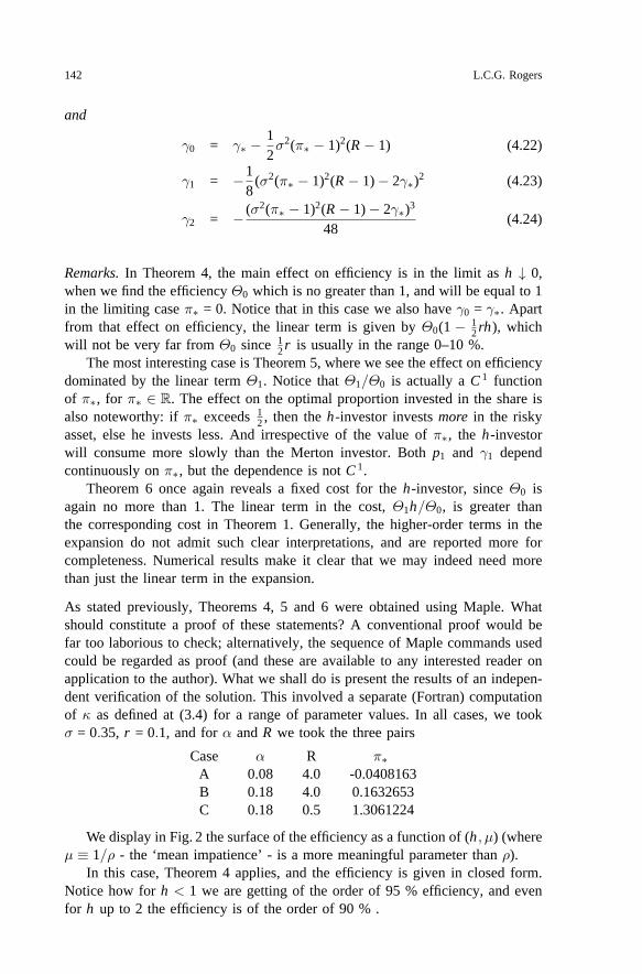
We display in Fig. 2 the surface of the efficiency as a function of (h, µ) (whereµ ≡ 1/ρ - the ‘mean impatience’ - is a more meaningful parameter thanρ).

In this case, Theorem 4 applies, and the efficiency is given in closed form.Notice how forh < 1 we are getting of the order of 95 % efficiency, and evenfor h up to 2 the efficiency is of the order of 90 % .

The relaxed investor 143

1

0.95

0.9

0.85

0.8

0.75

0.7

mu

108

64

2

h

5

4

3

2

1

0

Fig. 2. Plot of efficiency against µ = 1/ρ and h for the Merton consumption problem in case A

rho=8.0

Lag h

effic

ienc

y

0.0 0.2 0.4 0.6 0.8 1.0

0.4

0.6

0.8

1.0

rho=0.1

Lag h

effic

ienc

y

0.0 0.2 0.4 0.6 0.8 1.0

0.94

0.96

0.98

1.00

rho=1.0

Lag h

effic

ienc

y

0.0 0.2 0.4 0.6 0.8 1.0

0.92

0.94

0.96

0.98

1.00

rho=4.0

Lag h

effic

ienc

y

0.0 0.2 0.4 0.6 0.8 1.0

0.80

0.90

1.00

rho=8.0

Lag h

effic

ienc

y

0.0 0.2 0.4 0.6 0.8 1.0

0.4

0.6

0.8

1.0

Fig. 3. Plot of efficiency against lag, showing true values (marked as large dots) and the values ob-tained from the asymptotic formula using terms up to and including order h2 (plotted as a continuouscurve), for the Merton consumption problem in case B, with four different values of ρ

The next pictures Fig. 3 show the efficiency in case B for four values of ρ:0.1, 1, 4 and 8. The numerically computed values are given by the dots, and theasymptotic is shown by the continuous line. For the first two cases, the asymptoticis extremely good. For the third and fourth, the asymptotic is good certainly outto 2/ρ years, which is a long time in terms of the impatience parameter ρ. Noticehow the numerically computed values exhibit pronounced curvature, in contrastto the first two cases. This shows that there is sometimes need of higher-orderterms in the expansion than just the first. It is of interest to compare the size of

144 L.C.G. Rogers

1

0.9

0.8

0.7

0.6

0.5

0.4

mu

108

64

2

h

5

4

3

2

1

0

Fig. 4. Plot of efficiency against µ = 1/ρ and h for the Merton consumption problem in case C

the loss of efficiency for this case with the previous case of the wealth problem.There we lost 0.36% for lag of 4, here we lose ten times as much, 3.6%, for lag0.6 when ρ = 0.1 or 1, for lag 0.33 when ρ = 4, and for lag 0.20 when ρ = 8.Thus the h-effect on the consumption investor is much greater than on the wealthinvestor, though not very great even so.

Figure 4 displays the efficiency as a function of (h, µ) for case C. The effectof h up to a year is no worse than a 10 % loss of efficiency. An interestingfeature is that the efficiency is not monotone in ρ.

5 Why are the effects so small?

In both the Merton consumption problem and especially the Merton wealth prob-lem, we find that the effect of the h-delay is numerically very small; the relaxedinvestor is not losing very much. Why should this be?

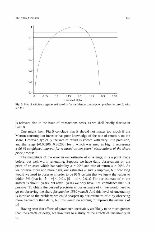
To understand this better, we display in Fig. 5 the efficiency of a Merton con-sumption investor who uses the wrong value for α in the Merton policy. Specif-ically, we suppose the parameters are as for Case B with ρ = 0.1, and that theinvestor puts a constant proportion (a − r)/σ2R of wealth into the share, andconsumes at rate (ρ+ (R −1)(r + (a − r)2/2Rσ2)/R times wealth. If a = 0.18, thetrue value of α, then the investor is following the Merton policy, otherwise he isbehaving suboptimally. The expression for the efficiency is easily derived fromthe expression (2.7) for the maximum payoff. Figure 5 shows also the levels 0.9and 0.95. We see that the efficiency drops off quite slowly from the maximum,being over 0.95 in the interval [0.10819,0.23000] and over 0.9 in the interval[0.07904,0.24761].

This then is a qualitative explanation of the small magnitude of the loss ofefficiency for the h-investor; even for moderately large values of h , it is unlikelythat the portfolio balance will be so far away from the Merton proportion to costtoo much. It is obvious once one sees it, but the efficiency as displayed in Fig. 5is a smooth function of a , and so near the maximum looks like a quadratic - adeparture from the Merton proportion of δ only incurs a loss of order δ2. This

The relaxed investor 145

0.350.30.250.20.150.10.050

1

0.9

0.8

0.7

0.6

0.5

0.4

Estimated alpha

Fig. 5. Plot of efficiency against estimated α for the Merton consumption problem in case B, withρ = 0.1

is relevant also to the issue of transactions costs, as we shall briefly discuss inSect. 8.

One might from Fig. 5 conclude that it should not matter too much if theMerton consumption investor has poor knowledge of the rate of return α on theshare. However, typically the rate of return is known with very little precision,and the range [-0.00206, 0.36206] for a which was used in Fig. 5 representsa 90 % confidence interval for α based on ten years’ observations of the shareprice process!!

The magnitude of the error in our estimate of α is huge; it is a point madebefore, but well worth reiterating. Suppose we have daily observations on theprice of an asset which has volatility σ = 20% and rate of return α = 20%. Aswe observe more and more days, our estimates σ and α improve, but how longwould we need to observe in order to be 95% certain that we knew the values towithin 5% (that is, |σ − σ| ≤ 0.01, |α − α| ≤ 0.01)? For our estimate of σ, theanswer is about 3 years; but after 3 years we only have 95% confidence that α ispositive! To obtain the desired precision in our estimate of α, we would need togo on observing the share for another 1530 years!! And this level of uncertaintyis intrinsic to the problem; we could sharpen up our estimates of σ by observingmore frequently than daily, but this would do nothing to improve the estimate ofα!

Having seen that effects of parameter uncertainty are likely to be much greaterthan the effects of delay, we now turn to a study of the effects of uncertainty inα.

146 L.C.G. Rogers

6 The impact of uncertainty on the wealth problem

In this section, we consider a Merton investor who may invest in the money-market account with constant interest rate r , and the share (2.1), but with thisdifference: the return parameter α is a random variable. We shall suppose thatdistribution of λ ≡ α/σ is N (λ0, v0), and in order that the problem be wellposed we have to assume that R > 1. The case of the Merton wealth problemis treated in a paper by Lakner (1995); we shall briefly summarize the relevantresults below. Much of the essential of the problem is covered also by Browneand Whitt (1996) in the case of logarithmic utility. Brennan (1998) derives thedynamics in the observation filtration, and finds an expression for the optimalinvestment rule in terms of a solution of a HJB equation. We shall make theoptimal rule explicit in what follows.

We shall investigate the cost of uncertainty, by comparing the maximisedexpected utility obtained by the investor who does not know the value of α (andso has to filter it from observations of the share) with the maximised expectedutility obtained by an investor who is told at time 0 what the (random) value ofα is, and who then follows the Merton optimal rule for that case.

The dynamics of the share price can be expressed as

dSt = σSt (dWt + λdt) (6.1)

= σSt dXt ,

so the uninformed investor attempts to filter the value of λ from observationsof Xt ≡ Wt + λt . We assume that λ and W are independent. This is a standardKalman filtering problem, whose solution is given by

dXt = dWt +v0Xt + λ0

1 + v0tdt (6.2)

where W is a Brownian motion in the observation filtration (Xt ). The distributionof λ conditional on (Xt ) is Gaussian with mean

λt ≡ v0Xt + λ0

1 + v0t

and variancevt ≡ v0

1 + v0t.

For more detail on the derivation of these results, see for example Bawa et al.(1979). The effect of this is that the investor is now investing in a risky assetwhose dynamics are given by (6.1) and (6.2). The change-of-measure martingalewhich converts X in (Xt ) into a Brownian motion with drift r/σ is

Zt ≡ (1 + v0t)1/2 exp

[−1

2v0

1 + v0tX 2

t +( r

σ− λ0

1 + v0t

)Xt

+t2

( λ20

1 + v0t− r2

σ2

)]. (6.3)

The relaxed investor 147

As is well known (see, for example, Karatzas (1989)), the optimal solution tothe Merton wealth problem with fixed horizon T is found by taking the marginalutility of terminal wealth w∗

T to be a multiple of the state-price density processζt ≡ e−rt Zt :

U ′(w∗T ) = γζT

for some γ chosen to match the initial wealth condition. In the case of CRRAutility U (c) = c1−R/(1 − R), we can compute everything explicitly 6, to obtain

sup E [U (wT )|w0 = w] = U (w)(

Eζ(R−1)/R)T

)R. (6.4)

Now a few calculations with the explicit expression (6.3) lead to

Eζ1−(1/R)T = e−r(R−1)T/R (1 + v0T )(R−1)/2R

(1 + cv0T )1/2exp

[− (λ0 − (r/σ))2cT

2R(1 + cv0T )

], (6.5)

where c ≡ 1 − (1/R), so that

sup E [U (wT )|w0 = w] = U (w)V (T , λ0, v0)

≡ U (w)(1 + v0T )(R−1)/2

(1 + cv0T )R/2.

exp

[− (λ0 − (r/σ))2cT

2(1 + cv0T )− r(R − 1)T

]. (6.6)

The optimal wealth process wt will satisfy

wt =γ−1/R

ζtEt ζ

1−(1/R)T ,

with optimal proportion πt to be invested in the risky asset being given as thecoefficient of dW in the expansion of dw/w. Here, Et denotes conditional ex-pectation given (Xt ). From this we find that

πt =(σλt − r)(1 + v0t)

σ2R(1 + v0T − (T − t)v0/R). (6.7)

As remarked by Brennan (1998), when R = 1 we find the standard Mertonrule, confirming the results of Feldman (1992). We also find that if the Mertonproportion is positive, then the derivative of πt with respect to R at R = 1 isnegative, exactly as one would expect, and in agreement with Brennan; the morerisk averse the agent, the less he will invest in the risky asset under uncertainty.Notice also that as t ↑ T , the investor is following more and more closely theMerton rule, and as T → ∞, the proportion of wealth in the risky asset goes tozero (unless R = 1); both of these conclusions seem intuitively reasonable.

6 The value function at an intermediate time will be a function of wt and λt . Since λ0 = λ0 isdeterministic, there is no need to make it explicit in the notation.

148 L.C.G. Rogers

Let us now compare with the investor who is told the value of λ at time 0,and who therefore follows the Merton rule. By time T he has made maximisedexpected utility (see (2.7))

U (w) exp[−T (R − 1)(r +

(λσ − r)2

2σ2R)]

(6.8)

which now has to be averaged over the random parameter λ which has a N (λ0, v0)distribution. After integrating, we find that the informed investor has maximisedexpected utility

U (w)

(R

R + (R − 1)Tv0

)1/2

exp

[− T (R − 1)((λ0σ − r)2 + 2rσ2{R + T (R − 1)v0}

2σ2(R + T (R − 1)v0)

].

The efficiency ΘI (T ) of the uninformed investor relative to the informed one isseen to be

ΘI (T ) =

(v0T (R − 1) + R

R(1 + v0T )

)1/2

=

(1 − T

R(τ + T )

)1/2

(6.9)

after some calculations. Here, we write τ ≡ 1/v0. In words, the agent who isinformed at time 0 of the true value of α can do as well with wealth ΘI (T ) as theinvestor who starts with wealth 1, but is given no information other than whathe can deduce from watching the price process.

Notice that the efficiency depends only on the time horizon T and the variancev0 of the initial estimate of λ0. What is the order of magnitude of the efficiency?Imagine the situation where an investor observes the price of the share for atime period of length τ before investing, and then uses the historical data toestimate λ (we make the situation easier by supposing that σ is known exactly).Then it is not hard to show that the variance of the estimator of λ0 is τ−1. Soa typical value for v0 would be somewhere in the range 0.5 to 5; observing forlonger would not necessarily help, since the mean return would not necessarilybe constant over long periods of time.

Figure 6 shows for a range of values of h the prior variance v0 that wouldbe required to give the same efficiency as the h-investor for the Merton wealthproblem. The plot contains results for time horizons T = 1, 4, 16 years. Asexpected, the prior variance at which the efficiencies match increases with h ,but the main thing to notice is the extremely small size of the values of v0 -even the highest point on the plot would require a prior variance of about 0.025,corresponding to 40 years’ worth of estimation data. For a 1-year horizon, withh = 1, we would need a prior variance of about 0.002, corresponding to about500 years’ worth of estimation data. This shows that the effect of parameteruncertainty on the Merton wealth problem is far more significant than the h-effect.

The relaxed investor 149

h

v_0

0 5 10 15

0.0

0.00

50.

010

0.01

50.

020

0.02

5

Fig. 6. Plot of the values of v0 required to give the same efficiency as the h-investor solving thewealth problem, with horizons T = 16 years (open circle symbol), T = 4 years (+) and T = 1 year(•). Parameters as in Case B

7 The impact of uncertainty on the consumption problem

The dynamics in the observation filtration of the asset price is once again givenby (6.1)–(6.2), with the state-price density once again given by the change-of-measure martingale (6.3) multiplied by the discount factor e−rt . As is wellknown (see, for example, Karatzas (1989)), the optimal solution to the problemis described in terms of the state-price density process ζ as

e−ρt U ′(c∗t ) = γζt (7.1)

for some constant γ chosen to match the budget constraint:

E∫ ∞

0ζt ct dt = w0. (7.2)

The budget constraint reworks to give

w0 = γ−1/RE∫ ∞

0e−ρt/Rζ

(R−1)/Rt dt

≡ γ−1/Rϕ(λ0, v0)

say, where

ϕ(λ0, v0) =∫ ∞

0

(1 + v0t)(R−1)/2R

(1 + cv0t)1/2exp

[− (λ0 − (r/σ))2ct

2R(1 + cv0t)− ρ + r(R − 1)

Rt

]dt .

There appears to be no simpler expression for ϕ. If we next consider the situationof the investor who is told at time 0 the true value α = σλ of the rate of return ofthe share, then the maximised objective of this agent will be obtained by firstlyconditioning on the value of α and then averaging over that value. What resultsis

150 L.C.G. Rogers

0.96

0.94

0.92

0.9

0.88

0.86

0.84

Mu

10

8

6

4

2

V_0

5

4

3

2

1

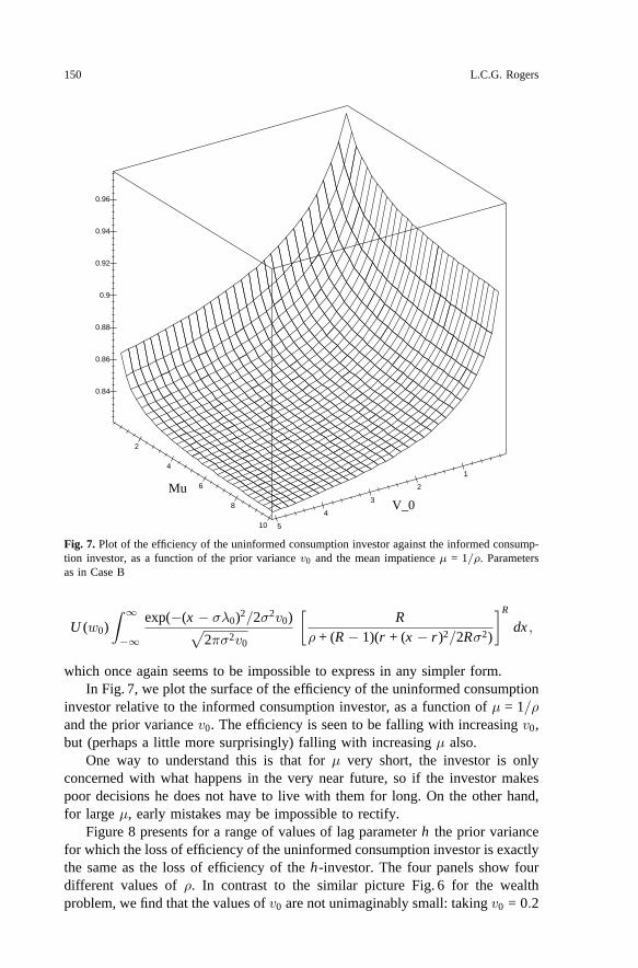
Fig. 7. Plot of the efficiency of the uninformed consumption investor against the informed consump-tion investor, as a function of the prior variance v0 and the mean impatience µ = 1/ρ. Parametersas in Case B

U (w0)∫ ∞

−∞

exp(−(x − σλ0)2/2σ2v0)√2πσ2v0

[R

ρ + (R − 1)(r + (x − r)2/2Rσ2)

]R

dx ,

which once again seems to be impossible to express in any simpler form.In Fig. 7, we plot the surface of the efficiency of the uninformed consumption

investor relative to the informed consumption investor, as a function of µ = 1/ρand the prior variance v0. The efficiency is seen to be falling with increasing v0,but (perhaps a little more surprisingly) falling with increasing µ also.

One way to understand this is that for µ very short, the investor is onlyconcerned with what happens in the very near future, so if the investor makespoor decisions he does not have to live with them for long. On the other hand,for large µ, early mistakes may be impossible to rectify.

Figure 8 presents for a range of values of lag parameter h the prior variancefor which the loss of efficiency of the uninformed consumption investor is exactlythe same as the loss of efficiency of the h-investor. The four panels show fourdifferent values of ρ. In contrast to the similar picture Fig. 6 for the wealthproblem, we find that the values of v0 are not unimaginably small: taking v0 = 0.2

The relaxed investor 151

•••••••••••••••••••••••••••••••••••••••••••••••••• • • • • • • •

••

•

•

•

Rho=0.1

h

v_0

0.0 0.5 1.0 1.5 2.0 2.5

0.0

0.2

0.4

0.6

0.8

1.0

••••••••••••••••••••••••••••••••••••••••••••••••••••

•••••• • • • • • • •

••

••

•

Rho=1

h

v_0

0.0 0.2 0.4 0.6 0.8 1.0

0.0

0.1

0.2

0.3

•••••••••••••••••••••••••••••••••••••••••••••••••••

••••••• • • • • • • •

••

••

•

Rho=4

h

v_0

0.0 0.05 0.10 0.15 0.20 0.25

0.0

0.10

0.20

•••••••••••••••••••••••••••••••••••••••••••••••••••

•••••• • • • • • • •

••

••

•

Rho=8

h

v_0

0.0 0.02 0.04 0.06 0.08 0.10 0.12

0.0

0.1

0.2

0.3

Fig. 8. Plots of the values of v0 required to give the same efficiency as the h-investor solving theconsumption problem for four different values of ρ. Parameters as in case B

(corresponding to an estimate based on 5 years’ data) we find that the loss ofefficiency is the same as for h = 1.6 for ρ = 0.1, h = 0.76 for ρ = 1, h = 0.2 forρ = 4, and h = 0.09 for ρ = 8.

As we see, these values are not unrealistic; h = 0.09 would correspond toan investor who would review his portolio about once a month. So the effect ofuncertainty and the h-effect are of similar order here, in contrast to the situationof the previous section, where we found that the effect of uncertainty was farlarger. Even so, we find that the effect of uncertainty is somewhat larger thanthe h-effect.

8 Conclusions and discussion

In this paper, we have modelled the effect of infrequent policy review, by allow-ing the agent to change his portfolio and consumption only at times which are amultiple of some positive h . 7 Taking as the natural yardstick the efficiency ofthe h-investor (that is, the quantity of money at time 0 which the ideal Mertoninvestor would require to gain the same payoff), we have shown that:

7 It might be argued that we should allow the agent to change consumption between reviews ofthe portfolio - the times when reviews take place are the only times the agent has access to themarket, but he can observe in the meantime what is going on. A problem of this kind is treated byRogers and Zane (1998).

152 L.C.G. Rogers

(8.1) the effect of infrequent policy review can be well approximated by a powerseries expansion in h , for both the wealth problem and the consumption problem;

(8.2) the magnitude of the effect is quite small in the consumption problem, andvery small for the wealth problem;

The small size of the effect is explained to some extent by the relative insensitivityof the payoff in the standard Merton problems to the policy used, as we have seen.This is related to results on transactions costs (see for example Constantinides1986, Davis and Norman 1990, Morton and Pliska 1995, Dumas and Luciano1991) where one finds that introducing a small transaction cost means that theoptimal policy for the Merton consumption investor involves very infrequentportfolio rebalancing. As is explained in Rogers (1999), the loss in the classicalproblem of Davis and Norman (1990) is made up of two components, the lossdue to the transactions costs, and the loss due to being imperfectly invested,which means that the value of the portfolio is not growing as fast as it would inthe ideal Merton situation. It turns out that these two losses are of comparablesize; our analysis here shows that the loss due to imperfect portfolio balance istypically small, and so therefore will be the loss due to transactions costs. Thisexplains qualitatively the fact that optimal rebalancing in the transactions costssituation is infrequent.8

The small size of the effect of imperfect portfolio balance led us to comparewith the magnitude of the effect of parameter uncertainty, especially in the rateof return. Here we were able to come up with the explicit form of the optimalportfolio choice (apparently for the first time) in the case where there is a priorGaussian distribution over the parameter.

By comparing the losses of efficiency due to the lag effect and due to pa-rameter uncertainty, we showed that:

(8.3) losses due to parameter uncertainty were far higher than the losses due tothe lag effect for the wealth problem, requiring prior estimates based on manydecades of data to match the lag effect for lags of several years;

(8.4) losses due to parameter uncertainty for the consumption problem were largerthan (but comparable with) the lag effect losses.

It appears then that the Merton wealth investor can be very relaxed; hislosses due to infrequent portfolio review are far smaller than likely losses due toparameter uncertainty. On the other hand, the Merton consumption investor canbe fairly relaxed about reviewing his portfolio, but he cannot neglect this effectin comparison with parameter uncertainty.

Appendix

Proof of Proposition 1 Through the proof, CN = CN (R, σ, α, r) denotes some con-stant whose value changes from line to line. By the Cauchy-Schwartz inequality,

8 If there is a proportional transaction cost δ, then the loss due to transactions costs in the problemconsidered by Davis and Norman (1990) is O(δ2/3) - see Shreve (1995) and Rogers (1999).

The relaxed investor 153

we have

E |(1 + θX )−R−2N X 2N +1| ≤(

E |1 + θX |−2R−4N

)1/2 (E |X |4N +2

)1/2

.

This gives us two terms to estimate. For the first,

E |1 + θX |−2R−4N

= E

[|1 + θX |−2R−4N : X ≥ 0

]+ E

[|1 + θX |−2R−4N : X < 0

]

≤ 1 + E

[(p exp(σWh + (α − σ2/2)h) + qerh )−2R−4N

]

≤ 1 + pE exp(−(2R + 4N )(σWh + (α − σ2/2)h)) + qe−(2R+4N )rh

≤ CN (R, σ, α, r).

For the second, we write ϕ(h) ≡ p(eαh − 1) + q(erh − 1). Notice thatsup0≤h≤1 h−1|ϕ(h)| < ∞. Thus

E |X |4N +2 = |peαh (eσWh−σ2h/2 − 1) + ϕ(h)|4N +2

≤ CN (R, σ, α, r)h2N +1,

for all 0 ≤ h ≤ 1, since by the Burkholder-Davis-Gundy inequalities (see, forexample, Rogers and Williams (1987), IV.42) E |eσWh−σ2h/2 − 1|j ≤ cj hj/2 forall h ∈ [0, 1]. �

References

1. Bawa, V. S., Brown, S. J., Klein, R. W.: Estimation risk and optimal portfolio choice. Amster-dam: North-Holland 1979

2. Brennan, M. J.: The role of learning in dynamic portfolio decisions. Europ. Finance Rev. 1,295–306 (1998)

3. Browne, S., Whitt, W.: Portfolio choice and the Bayesian Kelly criterion. Adv. Appl. Prob. 28,1145–1176 (1996)

4. Constantinides, G. M.: Capital market equilibrium with transaction costs. J. Polit. Econ. 94,842–862 (1986)

5. Davis, M. H. A., Norman, A. R.: Portfolio selection with transaction costs. Math. OperationsRes. 15, 676–713 (1990)

6. Dothan, M. U., Feldman, D.: Equilibrium interest rates and multiperiod bonds in a partiallyobservable economy. J. Finance 41, 369–382 (1986)

7. Dumas, B., Lucinao, E.: An exact solution to a dynamic portfolio choice problem with transactioncosts. J. Finance 46, 577–595 (1991)

8. Feldman, D.: Logarithmic preferences, myopic decisions and incomplete information. J. FinancialQuant. Anal. 27, 619–629 (1992)

9. Gennotte, G.: Optimal portfolio choice under incomplete information. J. Finance 41, 733–746(1986)

10. Hakansson, N. H.: Optimal investment and consumption strategies under risk for a class of utilityfunctions. Econometrica 38, 587–607 (1970)

11. Karatzas, I.: Optimisation problems in the theory of continuous trading. SIAM J. Control Optim.27, 1221–1259 (1989)

12. Karatzas, I., Zhao, X.: Bayesian adaptive portfolio optimisation. (Preprint) 1998

154 L.C.G. Rogers

13. Klein, R. W. Bawa, V. S.: The effect of estimation risk on optimal portfolio choice. J. FinancialEcon. 3, 215–231 (1976)

14. Klein, R. W., Bawa, V. S.: The effect of limited information and estimation risk on optimalportfolio diversification. J. Financial Econ. 5, 89–111 (1977)

15. Lakner, P.: Utility maximisation with partial information. Stoch. Proc. Appl. 56, 247–274 (1995)16. Lakner, P.: Optimal trading strategy for an investor: the case of partial information. (Preprint)

199817. Martini, C., Patry, C.: Variance optimal hedging in the Black-Scholes model for a given number

of transactions. (Preprint) 200018. Merton, R. C.: Lifetime portfolio selection under uncertainty: the continuous-time case. Rev.

Econ. Stat. 51, 247–257 (1969)19. Morton A. R., Pliska, S. R.: Optimal portfolio management with fixed transaction costs. Math.

Finance 5, 337–356 (1995)20. Rogers, L. C. G., Williams, D.: Diffusions, Markov Processes and Martingales, vol. 2. Chichester:

Wiley (1987)21. Rogers, L. C. G., Zane, O.: A simple model of liquidity effects. (Preprint) University of Bath

1998

Rogers, L. C. G.: Why is the effect of proportional transactions costs O(δ2/3)? (Preprint) Uni-versity of Bath 1999

22. Shreve, S. E.: Liquidity premium for capital asset pricing with transactions costs. In: Davis,M. H. A., Duffie, D., Fleming, W. H., Shreve S. E. (eds): Mathematical Finance: IMA Volumein Mathematics and its Applications 65. Berlin Heidelberg New York: Springer, pp. 117–133