The Operational Analysis of Queueing Network Models* PETER J. DENNING Computer Sciences Department, Purdue Unwers~ty, West Lafayette, Indiana 47907 JEFFREY P. BUZEN BGS Systems, Inc., Box 128, Lincoln, Massachusetts 01773 Queueing network models have proved to be cost effectwe tools for analyzing modern computer systems. This tutorial paper presents the basic results using the operational approach, a framework which allows the analyst to test whether each assumption is met in a given system. The early sections describe the nature of queueing network models and their apphcations for calculating and predicting performance quantitms The basic performance quantities--such as utilizations, mean queue lengths, and mean response tunes--are defined, and operatmnal relationships among them are derwed Following this, the concept of job flow balance is introduced and used to study asymptotic throughputs and response tunes. The concepts of state transition balance, one-step behavior, and homogeneity are then used to relate the proportions of time that each system state is occupied to the parameters of job demand and to dewce charactenstms Efficmnt methods for computing basic performance quantities are also described. Finally the concept of decomposition is used to stmphfy analyses by replacing subsystems with equivalent devices. All concepts are illustrated liberally with examples Keywords and Phrases" balanced system, bottlenecks, decomposability, operational analysis, performance evaluation, performance modeling, queuelng models, queuelng networks, response tunes, saturation. CR Categorws: 8.1, 4.3 INTRODUCTION Queueing networks are used widely to an- alyze the performance of multiprogrammed computer systems. The theory dates back to the 1950s. In 1957, Jackson published an analysis of a multiple device system wherein each device contained one or more parallel servers and jobs could enter or exit the system anywhere [JACK57]. In 1963 Jackson extended his analysis to open and closed systems with local load-dependent * This work was supported in part by NSF Grant GJ-41289 at Purdue University service rates at all devices [JACK63]. In 1967, Gordon and Newell simplified the no- tational structure of these results for the special case of closed systems [GORD67]. Baskett, et al. extended the results to in- clude different queueing disciplines, multi- ple classes of jobs, and nonexponential ser- vice distributions [BASK75]. The first successful application of a net- work model to a computer system came in 1965 when Scherr used the classical ma- chine repairman model to analyze the MIT time sharing system, CTSS [SCHE67]. How- ever, the Jackson-Gordon-Newell theory PermmsIon to copy without fee all or part of this material is granted provided that the copies are not made or distributed for direct commercial advantage, the ACM copyright notice and the titleof the publication and itsdate appear, and notice isgiven that copymg m by permission of the Assoclatlon for Computing Machinery. To copy otherwlse, or to republish, reqmres a fee and/or specificpermission. © 1978 ACM 0010-4892/78/0900-0225 Computing Surveys, Vol. 10, No. 3, September 1978

Welcome message from author
This document is posted to help you gain knowledge. Please leave a comment to let me know what you think about it! Share it to your friends and learn new things together.
Transcript
The Operational Analysis of Queueing Network Models*
PETER J. DENNING Computer Sciences Department, Purdue Unwers~ty, West Lafayette, Indiana 47907
JEFFREY P. BUZEN
BGS Systems, Inc., Box 128, Lincoln, Massachusetts 01773
Queueing network models have proved to be cost effectwe tools for analyzing modern computer systems. This tutorial paper presents the basic results using the operational approach, a framework which allows the analyst to test whether each assumption is met in a given system. The early sections describe the nature of queueing network models and their apphcations for calculating and predicting performance quantitms The basic performance quantities--such as utilizations, mean queue lengths, and mean response tunes--are defined, and operatmnal relationships among them are derwed Following this, the concept of job flow balance is introduced and used to study asymptotic throughputs and response tunes. The concepts of state transition balance, one-step behavior, and homogeneity are then used to relate the proportions of time that each system state is occupied to the parameters of job demand and to dewce charactenstms Efficmnt methods for computing basic performance quantities are also described. Finally the concept of decomposition is used to stmphfy analyses by replacing subsystems with equivalent devices. All concepts are illustrated liberally with examples
Keywords and Phrases" balanced system, bottlenecks, decomposability, operational analysis, performance evaluation, performance modeling, queuelng models, queuelng networks, response tunes, saturation.
CR Categorws: 8.1, 4.3
INTRODUCTION
Queueing networks are used widely to an- alyze the performance of multiprogrammed computer systems. The theory dates back to the 1950s. In 1957, Jackson published an analysis of a multiple device system wherein each device contained one or more parallel servers and jobs could enter or exit the system anywhere [JACK57]. In 1963 Jackson extended his analysis to open and closed systems with local load-dependent
* This work was supported in part by NSF Grant GJ-41289 at Purdue University
service rates at all devices [JACK63]. In 1967, Gordon and Newell simplified the no- tational structure of these results for the special case of closed systems [GORD67]. Baskett, et al. extended the results to in- clude different queueing disciplines, multi- ple classes of jobs, and nonexponential ser- vice distributions [BASK75].
The first successful application of a net- work model to a computer system came in 1965 when Scherr used the classical ma- chine repairman model to analyze the MIT time sharing system, CTSS [SCHE67]. How- ever, the Jackson-Gordon-Newell theory
PermmsIon to copy without fee all or part of this material is granted provided that the copies are not made or distributed for direct commercial advantage, the ACM copyright notice and the title of the publication and its date appear, and notice is given that copymg m by permission of the Assoclatlon for Computing Machinery. To copy otherwlse, or to republish, reqmres a fee and/or specific permission. © 1978 ACM 0010-4892/78/0900-0225
Computing Surveys, Vol. 10, No. 3, September 1978
226 P. J. Denning and J. P. Buzen
CONTENTS
INTRODUCTION 1 THE BASIS FOR OPERATIONAL ANALYSIS
Operatmnal Variables, Laws and Theorems Apphcatton Areas Prior Work m Operatmnal Analysts
2 VALIDATION AND PREDICTION 3 OPERATIONAL MEASURES OF NETWORKS
Types of Networks Bamc Operatmnal Quantities
4 JOB FLOW ANALYSIS Vtslt Ratms System Response Tune
Examples Bottleneck Analys~
Examples Summary
5 LOAD DEPENDENT BEHAVIOR 6 SOLVING FOR STATE OCCUPANCIES
State Trap~ttmn Balance Solving the Balance Equations
An Example Accuracy of the Analysm
7 COMPUTATION OF PERFORMANCE QUANTITIES Closed System with Homogeneous Service Tm~es Termmal Driven System with Homogeneous Serwce Tunes General Systems
8 DECOMPOSITON Offime Experiments Apphcatmns
CONCLUSIONS ACKNOWLEDGMENTS REFERENCES
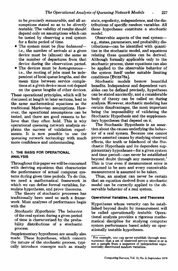
lay dormant until 1971 when Buzen intro- duced the central server model and fast computational algorithms for these models [BuzE71a, BuzE71b, BUZE73]. Working independently, Moore showed that queueing network models could predict the response times on the Michigan Terminal System (MTS) to within 10% [MooR71]. Extensive validations since 1971 have veri- fied that these models reproduce observed performance quantities with remarkable accuracy [BuzE75, GIAM76, HUGH73, LII's77, ROSE78]. Good surveys are [GELE76a, KLEI75, KLEI76, and MONT75].
Many analysts have experienced puzzle- ment at the accuracy of queueing network results. The traditional approach to deriv- ing them depends on a series of assump- tions used in the theory of stochastic proc- esses:
• The system is modeled by a stationary stochastic process;
• Jobs are stochastically independent; • Job steps from device to device follow
a Markov chain; • The system is in stochastic equilib-
rium; • The service time requirements at each
device conform to an exponential dis- tribution; and
• The system is ergodic--i.e., long-term time averages converge to the values computed for stochastic equilibrium.
The theory of queueing networks based on these assumptions is usually called "Markovian queueing network theory" [KLEI75]. The italicized words in this list of assumptions illustrate concepts that the an- alyst must understand to be able to deploy the models. Some of these concepts are difficult. Some, such as "equilibrium" or "stationarity," cannot be proved to hold by observing the system in a finite time period. In fact, most can be disproved empirically --for example, parameters change over time, jobs are dependent, device to device transitions do not follow Markov chains, systems are observable only for short pe- riods, service distributions are seldom ex- ponential. It is no wonder that many people are surprised that these models apply so well to systems which violate so many as- sumptions of the analysis!
In applying or validating the results of Markovian queueing network theory, ana- lysts substitute operational (i.e., directly measured} values for stochastic parameters in the equations. The repeated successes of validations led us to investigate whether the traditional equations of Markovian queueing network theory might also be re- lations among operational variables, and, if so, whether they can be derived using dif- ferent assumptions that can be directly ver- ified and that are likely to hold in actual systems. This has proved to be true [BuzE76a,b,c; and DENN77].
This tutorial paper outlines the opera- tional approach to queueing network modeling. All the basic equations and re- sults are derived from one or more of three operational principles:
• All quantities should be defined so as
Computing Surveys, Vol 10, No, 3, September 1978
The Operational Analysis of Queueing Network Models 227
to be precisely measurable, and all as- sumptions stated so as to be directly testable. The validity of results should depend only on assumptions which can be tested by observing a real system for a finite period of time.
• The system must be flow balanced-- i.e., the number of arrivals at a given device must be (almost) the same as the number of departures from that device during the observation period.
• The devices must be homogeneous-- i.e., the routing of jobs must be inde- pendent of local queue lengths, and the mean time between service comple- tions at a given device must not depend on the queue lengths of other devices.
These operational principles, which will be discussed at length in later sections, lead to the same mathematical equations as the traditional Markovian assumptions. How- ever, the operational assumptions can be tested, and there are good reasons to be- lieve that they often hold. This is why operational queueing network analysis ex- plains the success of validation experi- ments. It is now possible to use the queueing network technology with much more confidence and understanding.
1. THE BASIS FOR OPERATIONAL ANALYSIS
Throughout this paper we will be concerned with deriving equations that characterize the performance of actual computer sys- tems during given time periods. To do this, we need a mathematical framework in which we can define formal variables, for- mulate hypotheses, and prove theorems.
The theory of stochastic processes has traditionally been used as such a frame- work. Most analyses of performance begin with the
Stochastic Hypothesis: The behavior of the real system during a given period of time is characterized by the proba- bility distributions of a stochastic process.
Supplementary hypotheses are usually also made. These hypotheses, which concern the nature of the stochastic process, typi- cally introduce concepts such as steady
state, ergodicity, independence, and the dis- tributions of specific random variables. All these hypotheses constitute a stochastic model.
Observable aspects of the real system-- e.g., states, parameters, and probability dis- tributions--can be identified with quanti- ties in the stochastic model, and equations relating these quantities can be derived. Although formally applicable only to the stochastic process, these equations can also be applied to the observable behavior of the system itself under suitable limiting conditions [BuzE78a].
Stochastic models bestow bountiful benefits. Independent and dependent vari- ables can be defined precisely, hypotheses can be stated succinctly, and a considerable body of theory can be called on during analysis. However, stochastic modeling has certain disadvantages, the most important being the impossibility of validating the Stochastic Hypothesis and the supplemen- tary hypotheses that depend on it.
The Stochastic Hypothesis is an asser- tion about the causes underlying the behav- ior of a real system. Because one cannot prove asserted causes by studying observed effects, the truth or falsehood of the Sto- chastic Hypothesis and its dependent sup- plementary hypotheses--for a given system and time period--can never be established beyond doubt through any measurement. 1 This is true even if measurement error is assumed to be zero and every conceivable measurement is assumed to be taken.
Thus, an analyst can never be certain that an equation derived from a stochastic model can be correctly applied to the ob- servable behavior of a real system.
Operational Variables, Laws, and Theorems
Hypotheses whose veracity can be estab- lished beyond doubt by measurement will be called operationally testable. Opera- tional analysis provides a rigorous mathe- matical discipline for studying computer system performance based solely on oper- ationally testable hypotheses.
] For example, one can never establish through mea- surement that a set of observed service times ts or is not a sample from a sequence of independent expo- nentially distributed random variables.
Computing Surveys, Vol. 10, No. 3, September 1978
228 P. J. Denning and J. P. Buzen
In operational analysis there are two basic components to every problem: a sys- t em, which can be real or hypothetical, and a time period, which may be past, present, or future. The objective of an analysis is equations relating quantities measurable in the system during the given time period.
The finite time period in which a system is observed is called the observation period. An operational variable is a formal symbol that stands for the value of some quantity which is measurable during the observation period. It has a single, specific value for each observation period.
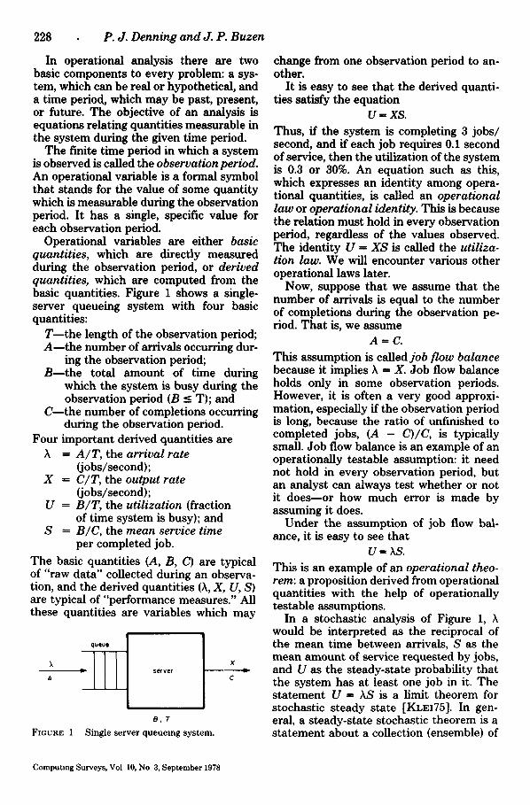
Operational variables are either basic quanti t ies, which are directly measured during the observation period, or derived quantit ies, which are computed from the basic quantities. Figure 1 shows a single- server queueing system with four basic quantities:
T-- the length of the observation period; A-- the number of arrivals occurring dur-
ing the observation period; B- - the total amount of time during
which the system is busy during the observation period (B _< T); and
C--the number of completions occurring during the observation period.
Four important derived quantities are ffi A / T , the arrival rate
(jobs/second); X = C/T , the output rate
(jobs/second); U ffi B / T , the uti l izat ion (fraction
of time system is busy); and S ffi B /C , the mean service t ime
per completed job.
The basic quantities (A, B, C) are typical of "raw data" collected during an observa- tion, and the derived quantities (~, X, U, S) are typical of "performance measures." All these quantities are variables which may
queue
FIGURE 1
s e r v e r
B,T
Single server queuelng system.
×
¢
change from one observation period to an- other.
It is easy to see that the derived quanti- ties satisfy the equation
U = XS.
Thus, if the system is completing 3 jobs/ second, and if each job requires 0.1 second of service, then the utilization of the system is 0.3 or 30%. An equation such as this, which expresses an identity among opera- tional quantities, is called an operational law or operat ional identity. This is because the relation must hold in every observation period, regardless of the values observed. The identity U = X S is called the utiliza- tion law. We will encounter various other operational laws later.
Now, suppose that we assume that the number of arrivals is equal to the number of completions during the observation pe- riod. That is, we assume
A ffi C.
This assumption is called job f low balance because it implies ~ ffi X. Job flow balance holds only in some observation periods. However, it is often a very good approxi- mation, especially if the observation period is long, because the ratio of unfinished to completed jobs, (A - C)/C, is typically small. Job flow balance is an example of an operationally testable assumption: it need not hold in every observation period, but an analyst can always test whether or not it does--or how much error is made by assuming it does.
Under the assumption of job flow bal- ance, it is easy to see that
U ffi AS.
This is an example of an operat ional theo- rem: a proposition derived from operational quantities with the help of operationally testable assumptions.
In a stochastic analysis of Figure 1, would be interpreted as the reciprocal of the mean time between arrivals, S as the mean amount of service requested by jobs, and U as the steady-state probability that the system has at least one job in it. The statement U = AS is a limit theorem for stochastic steady state [KLEI75]. In gen- eral, a steady-state stochastic theorem is a statement about a collection (ensemble) of
Computing Surveys, Vol 10, No 3, September 1978
The Operational Analysis of Queueing Network Models
possible infinite behavior sequences, but it is not guaranteed to apply to a particular finite behavior sequence. An operational theorem is a statement about the collection of behavior sequences, finite or infinite, that satisfy the given operational assump- tions: it is guaranteed to apply to every behavior sequence in the collection. (For detailed comparisons between stochastic and operational modeling, see [BouH78, BuzE78a].)
Application Areas
There are three major applications for op- erational results such as the utilization law:
• Performance Calculation. Operational results can be used to compute quan- tities which were not measured, but could have been. For example, a mea- surement of U is not needed in a flow- balanced system if k and S have been measured.
• Consistency Checking. A failure of the data to verify a theorem or identity reveals an error in the data, a fault in the measurement procedure, or a viola- tion of a critical hypothesis. For ex- ample, U ~ kS would imply an error if observed in a flow-balanced system.
• Performance Prediction. Operational results can be used to estimate per- formance quantities in a future time period (or indeed a past one) for which no directly measured data are avail- able. For example, the analyst can es- timate k and S for the future time period, and then predict that U will have the value kS in that time period. (Although the analyst may find ways of estimating U directly, it is often easier to calculate it indirectly from estimates of k and S.)
The first two applications are straightfor- ward, but the third is actually a two-step process. The first step is estimating the values of k and S for the future time period; the second step is calculating U. Our pri- mary concern in this paper is deriving the equations which can be used for perform- ance calculation, consistency checking, and the second step in performance prediction.
Parameter estimation, the first step in
229
performance prediction, is a problem of in- duction-inferring the characteristics of an unseen part of the universe on the basis of observations of another finite part. Gardner has an interesting discussion of why no one has found a consistent system of inductive mathematics [GARD76]. Various techniques for dealing with the parameter estimation problem will be discussed throughout this paper.
Prior Work in Operational Analysis
Many textbooks illustrate the ideas of prob- ability with operational concepts such as "relative frequencies" and "proportions of time." In addition, the derivations of many well-known results in the classical theory of stochastic processes are based, in part, on operational arguments. However, the ex- plicit recognition that operational analysis is a separate branch of applied mathemat- ics -qui te apart from the theory of stochas- tic processes--is a more recent develop- ment.
The concept of operational analysis as a separate mathematical discipline was first proposed by Buzen [BuzE76b], who char- acterized the real-world problems that could be treated with operational tech- niques, and derived operational laws and theorems giving exact answers for a large class of practical performance problems. At about the same time, operational argu- ments leading to upper and lower bounds on the saturation behavior of computer sys- tems were presented by Denning and Kahn [DENN75a]. These arguments were the op- erational counterpart of similar results de- veloped by Muntz and Wong [MUNT74]. The only operational assumption used at this point was job flow balance.
These early operational results dealt ex- clusively with mean values of quantities such as throughput, response time, and queue length. The theory was soon ex- tended so that complete operational distri- bu t ions-as well as mean values--could be derived for operational analogs of the "birth-death process" and the "M/M/1 queueing process" [BUzE76a, BUZE78a]. These extensions introduced two new analysis techniques: the application of
Computing Surveys, Vol. 10, No. 3, September 1978
230 P. J. Denning and J. P. Buzen
"flow balance" in the logical state space of the system (as contrasted with the physical system itself) and the homogeneity assump- tions, which are the operational counter- parts of Markovian assumptions in stochas- tic theory. These techniques form the basis for the operational treatment of many prob- lems which are conventionally analyzed with ergodic Markovian models.
The results in [BuzE76a and Buzz78a] applied only to single-resource queueing systems. The same analysis techniques were applied to multiple-resource queueing networks by Denning and Buzen [DENN77a], who showed that the "product form solution," encountered in Markovian queueing networks, holds in general queueing networks with flow balance and homogeneity; this result is more general than can be derived in the Markovian framework. This work also introduced a new operational concept, "online ffi offline behavior," which characterizes the way an- alysts use decomposition to estimate pa- rameters of devices and subsystems. The operational treatment of queueing network models is discussed in detail in the rest of this paper. Additional points about the the- ory and applications of operational analysis have been given in [BOUH78, BUZE77, BuzE78a].
2. VALIDATION AND PREDICTION
We have noted three uses of models in studying computer performance: calcula- tion, consistency-checking, and prediction of performance measures. Validation refers to extensive testing of a model to determine its accuracy in calculating performance measures. Predictzon refers to using a val- idated model to calculate performance measures for'a time period (usually in the future) when the values of parameters re- quired by the model are uncertain.
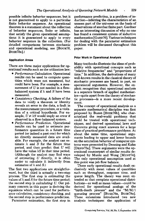
Figure 2 illustrates the steps followed in a typical validation. First, the analyst runs an actual workload on an actual system. For the observation period, he measures performance quantities, such as throughput and response time, and also the parameters of the devices and the workload. Then the analyst applies a model to these param- eters, and compares the results against the
measured performance quantities. If, over many different observation periods, the computed values compare well with actual (measured) values, the analyst will come to believe that the model is good. Thereafter, he will employ it confidently for predicting future behavior and for evaluating pro- posed changes in the system.
The scheme of Figure 2 is used to validate many types of models, including highly de- tailed deterministic models, simulation models, and queueing network models. In general, the more parameters used by the model, the greater is its accuracy in such validations.
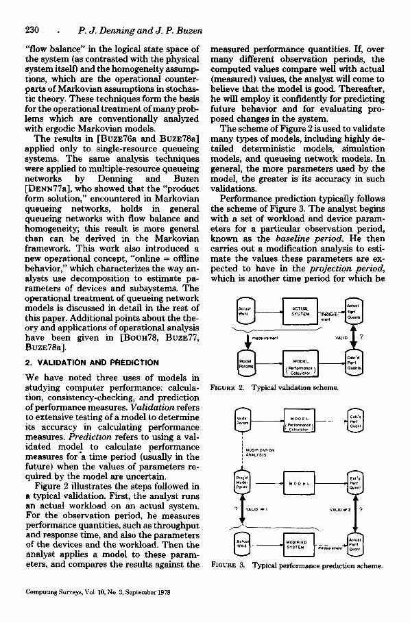
Performance prediction typically follows the scheme of Figure 3. The analyst begins with a set of workload and device param- eters for a particular observation period, known as the baseline period. He then carries out a modification analysis to esti- mate the values these parameters are ex- pected to have in the projection period, which is another time period for which he
~ ( ) meosurem4mt Per focmotce Col¢~ato~ MODEL VALID C~ Q P
FIGURE 2. Typical validation scheme.
?
MODIFICATION ANALYSIS
FIGURE 3. Typical performance prediction scheme.
Computing Surveys, Vol 10, No 3, September 1978
The Operational Analysis of Queueing Network Models
desires to know performance quantities. (In the projection period, the same system may be processing a changed workload, or a changed system may be processing the same workload, or both.) The analyst ap- plies the validated model to calculate per- formance quantities for the projection pe- riod. If the modification is ever imple- mented, the predictions can be validated by comparing the actual workload and system parameters against the project values (#1) and the actual performance quantities against the projected quantities (#2).
A variety of invariance assumptions are employed in the modification analysis. These assumptions are typically that device and workload parameters do not change unless they are explicitly modified--the an- alyst may assume, for example, that the mean disk service time will be invariant if the same disk is present in both the baseline and projection periods, or that the mean number of requests for each disk will be invariant if the same workload is present in both periods. Though usually satisfactory, such assumptions can lead to trouble if a given change has side effects--for example, increasing the number of time-sharing ter- minals may unexpectedly reduce the batch multiprogramming level even though the batch workload is the same.
The wise analyst will make all his invar- iance assumptions explicit. Otherwise, he will have difficulty in explaining a failure in Validation #1, which will cause a failure in Validation #2--even though previous tests of the model were satisfactory (Figure 2).
In some prediction problems there is no explicit baseline period. In these cases, the analyst must estimate parameters for the projection period by other means. For ex- ample, he can estimate the mean service time for a disk from published specifica- tions of seek time, rotation time, and data transfer rate; and he can estimate the mean number of disk requests per job from an analysis of the source code of representative programs. Usually, however, the modifica- tion analysis is more accurate when it be- gins with a measured baseline period.
A model's quality depends on the number of parameters it requires. The more infor- mation the model requires about the work-
231
load and the system, the greater the accu- racy attainable in its calculations. However, when there are many parameters, there may be a lot of uncertainty about whether all are correctly estimated for a projection period; the confidence in the predictions may thereby be reduced. Queueing network models isolate the few critical parameters. They permit accurate calculation and cred- ible prediction.
Additional issues of performance calcu- lation and parameter estimation will be dis- cussed as they arise throughout the paper. (See also [BuzE77, BUZE78a].)
3. OPERATIONAL MEASURES OF NETWORKS
Figure 1 illustrated a "single resource" queueing model consisting of a queue and a service facility. This model can be used to represent a single input/output (I/O) device or central processing unit (CPU) within a computer system. A model of the entire computer system can be developed by connecting single-resource models in the same configuration as the devices of an actual computer system. A set of intercon- nected single-resource queueing models comprises a multiple-resource queueing network.
Types of Networks
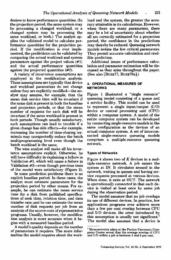
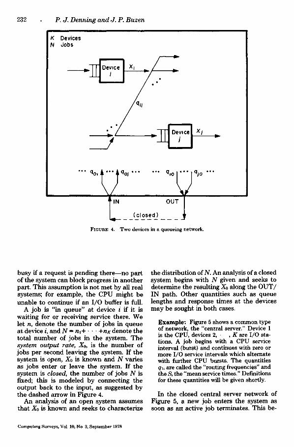
Figure 4 shows two of K devices in a mul- tiple-resource network. A job enters the system at IN. It circulates around in the network, waiting in queues and having ser- vice requests processed at various devices. When done, it exits at OUT. The network is operationally connected in that each de- vice is visited at least once by some job during the observation period.
The model assumes that no job overlaps its use of different devices. In practice, few applications programs ever achieve more than a few per cent overlap between CPU and I/O devices: the error introduced by this assumption is usually not significant. 2 The model also assumes that a device is
2 Measurements taken at the Purdue Umverslty Com- puter Center reveal that the average overlap of CPU and I/O within a job is between 4 and 6 per cent.
Computing Surveys, Vol 10, No 3, September 1978
232 P. J . D e n n i n g a n d J . P. B u z e n
K N
Devices Oobs
.~-~ Device [ X~ ~ / / ~
• • / qlJ
Xj
" ' " qo, I qoi . . . . . . qlo
IN OUT
( c l o s e d )
FIGURE 4. Two devices in a queueing network.
. . .
busy if a request is pending theremno part of the system can block progress in another part. This assumption is not met by all real systems; for example, the CPU might be unable to continue if an I/O buffer is full.
A job is "in queue" at device i if it is waiting for or receiving service there. We let n, denote the number of jobs in queue at device i, and N = n l + • • • +nK denote the total number of jobs in the system. The s y s t e m o u t p u t rate , Xo, is the number of jobs per second leaving the system. If the system is open, Xo is known and N varies as jobs enter or leave the system. If the system is closed, the number of jobs N is fixed; this is modeled by connecting the output back to the input, as suggested by the dashed arrow in Figure 4.
An analysis of an open system assumes that X0 is known and seeks to characterize
the distribution of N. An analysis of a closed system begins with N given and seeks to determine the resulting X0 along the OUT/ IN path. Other quantities such as queue lengths and response times at the devices may be sought in both cases.
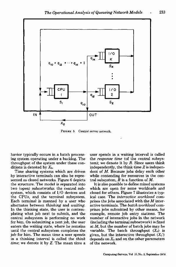
Example: Figure 5 shows a common type of network, the "central server." Device 1 is the CPU, devices 2, • , K are I/O sta- tions. A job begins with a CPU service interval (burst) and continues with zero or more I/O service intervals which alternate with further CPU bursts. The quantities qu are called the "routing frequencies" and the S, the "mean service times." Definitions for these quantities will be given shortly.
In the closed central server network of Figure 5, a new job enters the system as soon as an active job terminates. This be-
Computing Surveys, Vol 10, No 3, September 1978
The Operational Analysis of Queueing Network Models 233
IN
qlO + q12 + "" + q lK ffi I
Si qlo
Xo
q l K
SK
q l2 ~~--'~-~ S2
OUT
FIGURE 5. Centra l server network.
havior typically occurs in a batch process- ing system operating under a backlog. The throughput of the system under these con- ditions is denoted by X0.
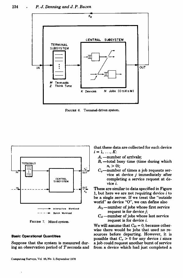
Time sharing systems which are driven by interactive terminals can also be repre- sented as closed networks. Figure 6 depicts the structure. The model is separated into two {open) subnetworks: the central sub- system, which consists of I/O devices and the CPUs, and the terminal subsystem. Each terminal is manned by a user who alternates between thinking and waiting. In the thinking state, the user is contem- plating what job next to submit, and the central subsystem is performing no work for him. On submitting a next job, the user enters the waiting state, where he remains until the central subsystem completes the job for him. The mean time a user spends in a thinking interval is called the think time; we denote it by Z. The mean time a
user spends in a waiting interval is called the response time (of the central subsys- tem); we denote it by R. Since users think independently, the think time Z is indepen- dent of M. Because jobs delay each other while contending for resources in the cen- tral subsystem, R is a function of M.
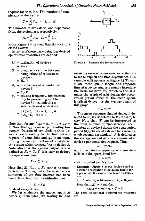
It is also possible to define mixed systems which are open for some workloads and closed for others. Figure 7 illustrates a typ- ical case. The interactive workload com- prises the jobs associated with the M inter- active terminals. The batch workload com- prises jobs submitted by other means, for example, remote job entry stations. The number of interactive jobs in the network (including the terminal subnetwork) is fixed at M, but the number of batch jobs may be variable. The batch throughput (Xo) is given, but the interactive throughput (Xo') depends on X0 and on the other parameters of the network.
Computmg Surveys, Vol 10, No. 3, September 1978
234 P. J. D e n n i n g a n d J. P. B u z e n
×;
TERMINAL SUBSYSTEM
- " ~ N ~
M Term,nols Z Think T,me
CENTRAL SUBSYSTEM
[ i OUT
K Devices N Jobs (O~N<-M)
FmURE 6. Termmal-driven system.
I TERMINALS
-' L __~ CENTRAL
SUBSYSTEM
OUT
OUT Xo
P interactive Workload -- -- -- ~ Batch Workload
FIGURE 7. Mixed sys tem.
Basic Operational Quantities
Suppose that the system is measured dur- ing an observation period of T seconds and
that these data are collected for each device i ffi 1 . . . . , K:
A, --number of arrivals; B, - - to ta l busy time (time during which
n, > 0); C,~--number of times a job requests ser-
vice at device j immediately after completing a service request at de- vice i.
These are similar to data specified in Figure 1, but here we are not requiring device i to be a single server. If we treat the "outside world" as device "O", we can define also
Aoj--number of jobs whose first service request is for device j;
C,o--number of jobs whose last service request is for device i.
We will assume that Coo = 0, because other- wise there would be jobs that used no re- sources before departing. However, it is possible that C, > 0 for any device i since a job could request another burst of service from a device which had just completed a
Computing Surveys, Vol 10, No 3, September 1978
The Operational Analysis of Queueing Network Models
request for tha t job. The number of com- pletions at device i is
K C,=ECv, t = l . . . . . K.
j - -0
The number of arrivals to, and departures from, the system are, respectively,
K K
A0 = ~ Ao~, Co=~C,o. j --1 t - I
From Figure 4 it is clear tha t Ao = Co in a closed system.
In terms of these basic data, four derived operational quantit ies are defined:
U, ffi utilization of device i = B , / T .
S, ffi mean service t ime between completions of requests at device i
= B,/C~
X, = output rate of requests from device i
= C , / T qu ---- routing frequency, the fraction
of jobs proceeding next to device j on completing a service request at device i
fC , /C , , i f / - - 1 . . . . . K = "--LAoj/Ao, if i = 0.
nt(t) A / \
B,
( t )
6
5
4-
3-
2 .
I -
0 5 I0 15 20
FIGURE 8. Example of a device's operation.
Note that , for any i, q,o + qtl + . . . + qtK =
1. Note tha t q,0 is an output routing fre- quency (fraction of completions from de- vice i corresponding to the final service request of some job) and q0j is an input routing f requency (fraction of arrivals to the system which proceed first to device j) . Note also tha t the system output rate is defined as Xo -- Co/T. It is easy to deduce the operational law
K
Xo = ~ X,q,o. t - 1
Note tha t X0, X1 . . . . . . X r cannot be inter- preted as " throughputs" because no as- sumption of job flow balance has been made. I t is clear tha t the utilization law
U, = X,S, holds at every device.
We let n, denote the queue length at device i; it includes jobs waiting for and
235
receiving service. Somet imes we write n,(t) to make explicit the t ime dependence. (An example n,(t) appears in Figure 8.) To cal- culate mean queue length and response t ime at a device, analysts usually introduce the basic measure W,, which is the area under the graph of n,(t) during the obser- vation period. Since f~,, the mean queue length at device i, is the average height of this graph,
ft, = WJT.
The mean response t ime at device i, de- noted by R,, is also related to W, in a simple way. Note tha t W~ can be interpreted as the total number of "job-seconds" accu- mula ted at device i during the observation period ( if j jobs are at a device for s seconds, j s job-seconds accumulate). R, is defined as the average amount of t ime accumulated at device i per completed request. Thus
R, = W,/C,.
An immediate consequence of these defi- nitions is the operational law
6, = X~R,,
which is called Little's Law. Example: Figure 8 shows device t and a possible observation of its queue length for a period of 20 seconds. The basic measures a r e
A, = 7 jobs, B, = 16 seconds, C, ffi 10 jobs. Note that n,(0) ffi 3 and that
n,(20) ffi n,(0) + A, - C~ = 0. The basic operational performance measures a r e
Comput ing Surveys, Vol 10, No. 3, September 1978
236 P. J. Denning and J. P. Buzen
U, -- 16 /20 St = 1 6 / 1 0 X, ffi 1 0 / 2 0
= 0.80 --- 1.6 -- 0.5
seconds jobs/second The total area under n,(t) in the observation period is
W~ -- 40 job-seconds. Thus the mean queue length is
ht = W,/T ffi 2 jobs, and the mean response time per service completion is:
R, ffi WJC, = 4 seconds.
4. JOB FLOW ANALYSIS
Given the mean service times (S,) and the routing frequencies (q,j), how much can we determine about overall device completion rates (XJ or response times (RJ? These questions are usually approached through the operational hypothesis known as the
Prmciple of Job Flow Balance: For each device i, Xt is the same as the total input ra te to device i.
This principle will give a good approxima- tion for observation periods long enough tha t the difference between arrivals and completions, At - C, is small compared to C~. I t will be exact if the initial queue length n~(0) is the same as the final n,(T). Choosing an observation period so that the initial and final states of every queue are the same is not as strange as it might seem. This notion underlies the highly successful "regenera- tion point" method of conducting simula- tions [IGLE78].
When job flow is balanced, we refer to the X, as device throughputs. Expressing the balance principle as an equation,
K
C j f A j = Z C,j, t = O . . . . g t--O
(Note tha t job flow balance allows us to substi tute Coj for Ao~.) With the definition qtj = CJC, , we may write
K
Cj = E C,q,j. tmO
Employing the definition X~ ffi C,/T, we obtain
JOB FLOW BALANCE EQUATIONS K
X+ffi Y,X,q,~, /ffiO . . . . . g tmO
If the network is open, the value of X0 is externally specified and these equations will have a unique solution for the un- knowns X,. However, if the network is closed, Xo is initially unknown, and the equations have no unique solution; this can be verified by showing tha t the sum of the Xj-equations f o r j ffi 1 . . . . , K reduces to the Xo-equation. In a closed network, there are K independent equations but K + 1 un- knowns. Nonetheless, the job flow balance equations contain information of consider- able value.
Visit Ratios
T h e "visit ratio," which expresses the mean number of requests per job for a device, can always be calculated uniquely from the job flow balance equations. With the mean ser- vice times, they can be used to determine the throughputs and response t imes of sys- tems under very light or very heavy loads. Define
V, = X , /Xo;
V~ is the job flow through device t relative to the system's ou tput flow. Our definitions imply tha t V, ffi C,/Co, which is the mean number of completions at device i for each complet ion f rom the system. Since V, can be interpreted as the mean number of visits per job to device i, we call it the visit ratio.
The relation X, ffi V, Xo is an operational law, called the Forced Flow Law. It s tates tha t the flow in any one par t of the system determines the flows everywhere in the sys- tem.
E x a m p l e : Consider the performance ques- tion: "Jobs generate an average of 5 disk requests and disk throughput is measured as 10 requests/second; what is the system throughput?" This question seems momen- tartly frivolous, since nothing is stated about the relation between the disk and any other part of the system. Yet the forced flow law gives the answer precisely. Let subscript t refer to the disk:
Xo ffi X,/ V, ffi 10 requests/second
5 requests/job ffi 2 jobs/second.
On replacing each X, with V, Xo in the job flow balance equations, we obtain the
Computmg Surveys, Vol. 1O, No. 3, September 1978
T h e O p e r a t i o n a l A n a l y s i s o f Q u e u e i n g N e t w o r k M o d e l s
VISIT RATIO EQUATIONS 170=1
K
V~=qoj+ ~ V,q,j, 1 = 1 . . . . . K
These are K + 1 independent equations with K + 1 unknowns: a unique solution is always possible assuming the network is operationally connected. These equations show the relation between the network's "connective structure," represented by the q,j, and the visit ratios. Although V~ = X, /Xo is an operational law, the iT, satisfy the visit ratio equations only if job flow is balanced in the network.
Example: The central server network (Figure 5) has these job flow equations:
Xo = Xlqlo
XI f Xo + X2 + . . . + X~
X ,=XIqI , , iffi2 . . . . . K.
Setting X, = V, Xo, these equations reduce to
1 = Vlqlo
V]= I + V2+ . . . + VK
V , = Vlq~,, t = 2 . . . . . K .
It is easy to see that
V1 -- 1/qlo
V, = ql,/qlo, i = 2 . . . . . K.
In this case, only K of the possible routing frequencies q~j are nonzero; these q~, can be determined uniquely if the 17, are given. This is not so in a general network, where K visit ratios are insufficient to determine the (K + 1) 2 unknown routing frequencies.
As we shall see, all the performance quan- tities can be computed using only the visit ratios and the mean service times S, as parameters. The visit ratio equations are used to prove tha t this is so. In practice, the analyst may be able to extract the visit ratios directly from workload data, thereby avoiding computing a solution of the visit ratio equations.
System Response Time
One method of computing the mean re- sponse t ime per job, R, for an open or closed system is to apply Little 's law to the system as a whole,
R = ~ f /Xo ,
237
where fil = fh + . . . + fix. I f /g/or Xo are not known, an al ternate me thod can be used. Since h, = X,R, from Little 's law at device i, and X, = V, Xo from the forced flow law, we have f i , /Xo = V,R,. This reduces [V/Xo to the G e n e r a l R e s p o n s e T t m e Law:
K
R f Y. V~R,. t l l
This law holds even if job flow is not bal- anced.
Little 's law can be used to compute the central subsystem's response t ime R in the terminal driven system of Figure 6. Th e mean time for a user to complete a think- wait cycle is Z + R. When job flow is balanced, X0 will denote the rate at which cycles are completed. By Little 's law, (Z + R)Xo must be the mean number of users observed to be in a think-wait cycle; but all the users are in such cycles, hence, M = (Z + R)Xo. Therefore ,
R ffi M / X o - Z .
This is called the I n t e r a c t i v e R e s p o n s e T i m e F o r m u l a .
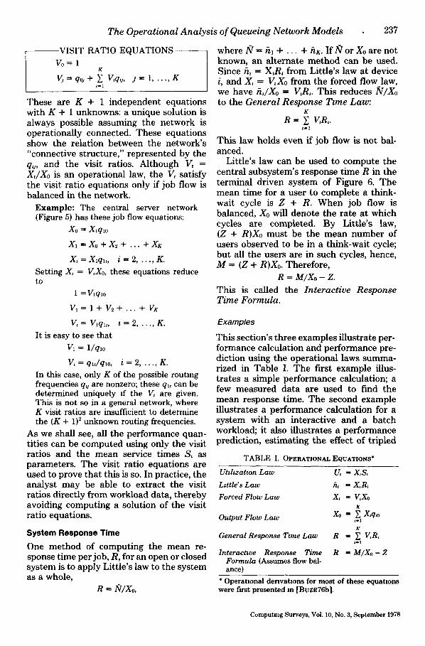
Examples
This section's three examples illustrate per- formance calculation and performance pre- diction using the operational laws summa- rized in Table I. The first example illus- t rates a simple performance calculation; a few measured data are used to find the mean response time. The second example illustrates a performance calculation for a system with an interactive and a batch workload; it also illustrates a performance prediction, estimating the effect of tripled
TABLE I. OPERATIONAL EQUATIONS*
Utthza t ton L a w U, = X,S,
Ltttle' s L a w f~ ffi X ,R,
Forced F low L a w X~ ffi V, Xo K
Output F low L a w Xo ffi ~ X,q,o
K
General Response T tme L a w R ffi ~ V,R,
In teract tve Response T ime R - M/Xo - Z Formula (Assumes flow bal- ance)
* Operational derivations for most of these equations were fLrst presented In [BuzE76b].
Computmg Surveys, Voi. 10, No. 3, September 1978
238 P. J . D e n n i n g a n d J. P. B u z e n
batch throughput on interactive response time. The third example illustrates a more complex prediction problem, estimating the effect of consolidating two separate time sharing systems; it illustrates the use of invariance assumptions in the modification analysis.
For the first example, we suppose that these data have been measured on a time sharing system:
Each job generates 20 disk requests; The disk utilization is 50%; The mean service time at the disk is 25
milliseconds; There are 25 terminals; and Think time is 18 seconds.
We can calculate the response time after first calculating the throughput. Let sub- script i refer to the disk. The forced flow and utilization laws imply
Xo = X, /V , ffi u J v , s,.
From the data, (.5)
Xo ffi - - ffi 1 job/second. (20)(.025)
From the interactive response time for- mula,
R ffi 20/1 - 18 ffi 2 seconds.
Our second example considers a mixed system of the type shown in Figure 7. These data are collected:
There are 40 terminals; Think time is 15 seconds; Interactive response time is 5 seconds; Disk mean service time is 40 milliseconds; Each interactive job generates 10 disk
requests; Each batch job generates 5 disk requests;
and Disk utilization is 90%.
We would like to calculate the throughput of the batch system and then estimate a lower bound on interactive response time assuming that batch throughput is tripled. The interactive response time formula gives the interactive throughput:
Xo' ffi M / ( Z + R') ffi 40/(15 + 5) ffi 2 jobs/second.
Let subscript i refer to the disk. The disk throughput is X, + X,', where X, is the batch component and X / i s the interactive com- ponent. The utilization law implies
X, + X ; ffi U,/S, ffi (.9)/(.04) ffi 22.5 requests/second.
The forced flow law implies that the inter- active component is
X," ffi V,'Xo' ffi (10)(2) ffi 20 requests/second,
so that the batch component is
X, -- 22.5 - 20 ffi 2.5 requests/second.
Using the forced flow law again, we find the batch throughput:
Xo ffi X J V , ffi 2.5/5 ffi 0.5 jobs/second.
Now consider the effect of tripling the batch throughput. If X0 were changed to 1.5 jobs/second without changing V, then X, would become V~0 ffi 7.5 requests/second. Assuming that the increased throughput does not change the disk service time, the maximum completion rate at the disk is 1/S~ ffi 25 requests/second; this implies that the completion rate of the interactive work- load, X/, cannot exceed 25 - 7.5 ffi 17.5 requests/second. Therefore
Xo' = X , ' /V ; <- 17.5/10 ffi 1.75 jobs/second
and
R' ffi M/Xo" - Z >_ 40/1.75 - 15 ffi 7.9 seconds.
Tripling batch throughput increases inter- active response time by at least 2.9 seconds.
Notice that the validity of these esti- mates depends on the assumptions that the parameters M, Z, 11,, and S, are invariant under the change of batch throughput. Al- though these are often reasonable assump- tions, the careful analyst will check them by verifying that the internal policies of the operating system do not adjust to the new load, and that interactive users are inde- pendent of batch users.
For the third example, we consider a computer center which has two time shar-
Computing Surveys, Vol 10, No. 3, September 1978
The Operatmnal Analysis of Queueing Network Models
ing systems; each is based on a swapping disk whose mean service t ime per request is 42 msec. The mean think t ime in both systems is Z - 15 seconds. These data have been collected:
System A System B 16 terminals 10 terminals 25 disk requests/job 16 disk requests/job 80% disk utilization 40% disk utilization
In order to reduce disk rentals, manage- ment is proposing to consolidate the two systems into one with 26 terminals and using only one of the disks. We would like to est imate the effect on the response t imes for the two classes of users.
We let subscript i refer to the disk, and use primed symbols to refer to System B. T he formula X0 = U,/V~S, gives through- puts for the two systems:
(.8) X o - - - -
(25)(.042) = 0.77 jobs/second (System A)
(.4) Xo'
(16)(.042) = 0.60 jobs/second (System B)
The response t imes are
R --- 16/(.77) - 15 = 5.8 seconds (System A)
R'ffi 10/(.6) - 15
= 1.1 seconds (System B)
Over an observation period of T seconds there would be X,T disk requests serviced in Sys tem A, and X { T in System B; the fraction of all disk requests which are A- requests would be
X~T/(X,T + X{T) ffi U,/(U, + U{) = 2/3.
In order to est imate the effect of consol- idation, we need to know the disk comple- t ion rates for each workload when both workloads share the one disk. Because the characteristics of the users and the disk are the same before and after the change, it is reasonable to make this invariance assump- tion: In the consolidated system, 2/3 of the disk requests will come from the A-users. I t is also reasonable to assume tha t the disk utilization will be nearly 100% in the con- solidated system. This implies tha t the total disk throughput will be 1/S, -- 1/(.042) =
239
24 requests/second. Of this total, the throughputs of the two types of users are
X, = (2/3)(24) = 16 requests/second (A-users)
X{= (1/3)(24) ffi 8 requests/second (B-users)
This implies tha t the system throughputs are
Xo = XJV~ = 16/25 ffi 0.64 jobs/second (A-users)
Xo' = X/ /V/ = 8/16 -- 0.5 jobs/second (B-users)
and tha t the response t imes are
R = 16/(.64) - 15 = 10 seconds (A-users)
R ' = 10/(.5) - 15 = 5 seconds (B-users)
Note tha t the two types of users experience different response times. This is because the B-users, who generate less work for the disk, are delayed less at the disk than the A-users.
Once again it is worth noting explicitly tha t the parameters V,, ]7,', S,, and Z are assumed to be invariant under the proposed change. The careful analyst will check the validity of these assumptions. Th e assump- tion tha t the ratio of Sys tem A to System B throughputs is invariant under the change should be approached with caution; it is typical of the assumptions a skilled analyst will make when given insufficient data about the problem. We will present an example shortly in which a faster CPU af- fects two workloads differently: the ratio of interactive to batch th roughput changes.
Bottleneck Analysis This section deals with the asymptot ic be- havior of th roughput and response t ime of closed systems as N, the number of jobs in the system, increases. We will assume tha t the visit ratios and mean service t imes are invariant under changes in N.
Note tha t the ratio of complet ion rates for any two devices is equal to the ratio of their visit ratios:
Computmg Surveys, Voi. 10, No. 3, September 1978
240 P. J. Denning and J. P. B u z e n
X, IXj = V, IV~.
Since/.7, ffi X,S,, a similar property holds for utilizations:
u , / v ~ = v , s , / y ~ s , .
Our invariance assumptions imply that these ratios are the same for all N.
Device i is sa turated if its utilization is approximately 100%. If U, ffi 1, the utiliza- tion law implies that
X, = l / S , ;
this means that the saturated device is com- pleting work at its capacity--an average of one request each S, seconds. In general, U, -< 1 and X, <_ 1/S,.
Let the subscript b refer to any device capable of saturating as N becomes large. Such devices are called bottlenecks because they limit the system's overall performance. Every network has at least one bottleneck.
Since the ratios U,/Uj are fixed, the de- vice i with the largest value of V,S, will be the first to achieve 100% utilization as N increases. Thus we see that, whenever de- vice b is a bottleneck,
VbSb ffi max { V1S, ..... VKSK}.
The bottleneck(s) is (are) determined by device and workload parameters.
Now: if N becomes large we will observe Ub = 1 and Xb ffi 1/Sb; since Xo/Xb ffi 1/Vb, this implies
Xo-..= 1 /VbSb
is the maximum possible value of system throughput. Since V,S, is the total of all service requests per job for device i, the s u m
Ro ffi V,S, + + VKSK,
which ignores queueing delays, denotes the smallest possible value of mean response time. In fact, Ro is the response time when N = i. This implies that Xo = I/Ro when N = I .
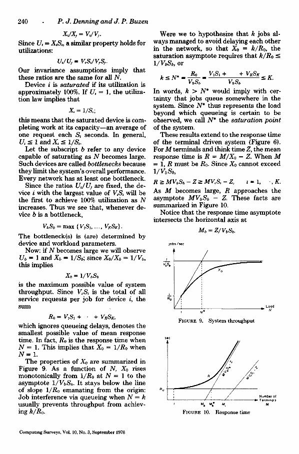
The properties of Xo are summarized in Figure 9. As a function of N, Xo rises monotonically from I/Ro at N -- 1 to the asymptote I/VbSb. It stays below the line of slope i/Ro emanating from the origin: Job interference via queueing when N ffi k usually prevents throughput from achiev- ing k/Ro.
Were we to hypothesize that k jobs al- ways managed to avoid delaying each other in the network, so that Xo ffi k/Ro, the saturation asymptote requires that k /Ro <-- 1/ VbSb, or
k < N* ffi Ro = V'S' + + VrSr - - VbSb VbSb -= K.
In words, k > N* would imply with cer- tainty that jobs queue somewhere in the system. Since N* thus represents the load beyond which queueing is certain to be observed, we call N* the saturation po in t of the system.
These results extend to the response time of the terminal driven system (Figure 6). For M terminals and think time Z, the mean response time is R = M/Xo - Z. When M ffi 1, R must be Ro. Since Xo cannot exceed l / V b S b ,
R >_ M V b S b - Z >- M V , S, - Z, l f f i l , - ,K .
As M becomes large, R approaches the asymptote MVbSb - Z. These facts are summarized in Figure 10.
Notice that the response time asymptote intersects the horizontal axis at
Mb = Z/VbSb.
lObS/sec
vbs,
L o a d D
I N ~' N
FIGURE 9. System throughput
Ro / / I Number of i Iv Termlno~$ l M~ M~ M M
FIGURE I0. Response time
Computing Surveys, Vol. 10, No. 3, September 1978
The Operational Analysis
This is a product of a waiting time at the terminals (Z) and a saturation job flow through the terminals (1/VbSD; by Little's law, Mb denotes the mean number of think- ing terminals when the system is saturated. The response time asymptote crosses the minimum response time R0 at
Mb* = (Ro + Z}/VbSb = N* + Mb.
when there are more than Mb* terminals, queueing is certain to be observed in the central subsystem.
Notice that the response time asymp- totes and intersections M0 and M0* depend only on M, Z, V0, and S0. The only assump- tions needed to compute them are job flow balance and invariance of the visit ratios and mean service times under changes in load. Note also that when Z = 0 these results yield the response time asymptotes of a closed central system. These results may be extended to include the case where service times are not strictly invariant, but each S, approaches some limit as the queue length at device i increases [MUNT74, DENN75a].
To summarize: the workload parameters or the visit ratio equations allows the ana- lyst to determine the visit ratios, V,. Device characteristics allow determination of the mean service time per visit, S,. The largest of the products V,S, determines the bottle- neck device, b. The sum of these products determines the smallest possible response time, R0. The system throughput is 1/VoSb in saturation. The saturation point N* of the central subsystem is Ro/VbSb; and N* + Z/VoSo terminals will begin to satu- rate the terminal driven system.
An analysis leading to sketches such as Figures 9 and 10 may give some gross guid- ance on effects of proposed changes. For example, reducing V,S, for a device which is not a bottleneck (e.g., by reducing the service time or the visit ratio) will not affect the bottleneck; it will make no change in the asymptote 1/VoSo and will generally produce only a minor change in minimal response time R0. Reducing the product V,S, for all the bottleneck devices will re- move the bottleneck(s); it will raise the asymptote 1/VbS0 and reduce R0. However, this effect will be noticed only as long as VbSb remains the largest of the V,S,: too
of Queueing Network Models 241
much improvement at device b will move the bottleneck elsewhere. These points will be illustrated by the example of the next section.
The property that 1/VbSb limits system throughput was observed by Buzen for Markovian central server networks [BvzE71a]. It was shown to hold under very general conditions by Chang and Laven- berg [CHAN74]. Muntz and Wong used it in bottleneck analysis of general stochastic queueing networks [MUNT74, MUNT75]; Denning and Kahn derived the operational counterpart [DENN75a]. Response time asymptotes were observed by Scherr for his model of CTSS [SCHE67], and by Moore for his model of MTS [Moon71]. The concept of saturation point was introduced by Kleinrock [KLEI68], who also studied all these results in detail in his book [KLEI76].
Examples
This section illustrates the applications of bottleneck analysis for the three cases of Figures 11 through 13. For each, we con- sider a series of questions as might be posed by a computing center's managers, who seek to understand the present system and to explore the consequences of proposed changes.
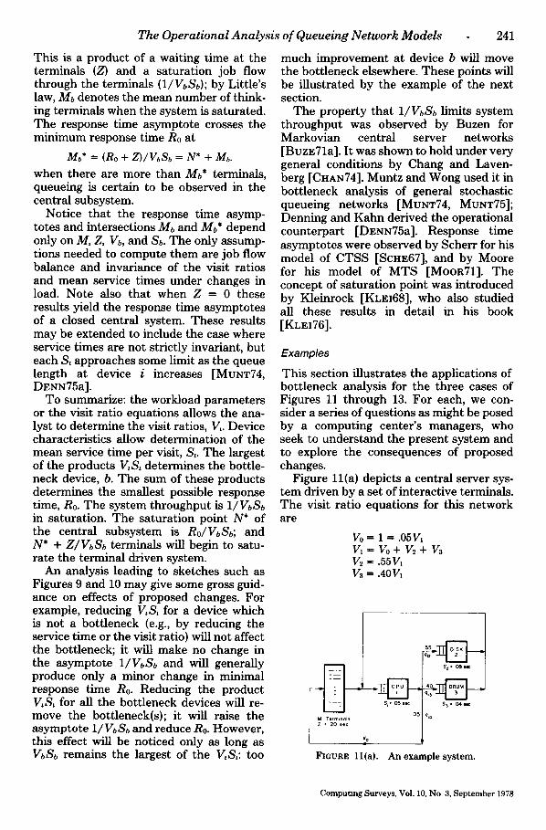
Figure ll(a) depicts a central server sys- tem driven by a set of interactive terminals. The visit ratio equations for this network are
V0 = 1 = .05VI Vl = Vo + V~ + V3 v2 = .55V, V3 = .40V~
i FIGURE ll(a).
q J2
Q*a
$a " 04t .~
An example system.
Computing Surveys, Vol. 10, No 3, September 1978
242
Sec,
2.2 -;
P. J. Denning and J. P. Buzen
i j / / I 20 22
Ms Mi }*
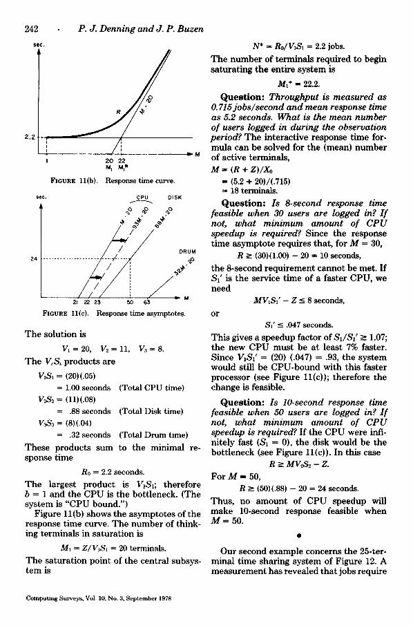
FIGURE l l (b ) . Response t ime curve.
~ M
CPU DISK sec.
24 . . . . . . . . . . . . . . . . . . . . . . . . / / DRUM
-- %0
~ M 21 22 23 50 63
FIGURE 11(C). Response t ime asymptotes.
T h e solution is
V1=20, V ~ = l l , V3=8.
T h e V,S, products are
V~S~ = (20)(.05) ffi 1.00 seconds (Total CPU time)
V2S2 = (11)(.08) -- .88 seconds (Total Disk time)
V~S3 ffi (8)(.04)
= .32 seconds (Total Drum time)
These products sum to the minimal re- sponse t ime
R0 ffi 2.2 seconds.
T h e largest product is ~S1; therefore b ffi 1 and the C P U is the bott leneck. (The sys tem is " C P U bound.")
Figure 11(b) shows the a sympto tes of the response t ime curve. T h e num ber of think- ing terminals in sa tura t ion is
M1 = Z/VISI = 20 terminals.
T h e sa tura t ion point of the central subsys- t em is
N* ffi Ro/V]S1 = 2.2 jobs.
T h e n u m b e r of terminals required to begin sa tura t ing the ent i re sys tem is
Ml* ffi 22.2.
Q u e s t i o n : Throughput is measured as O. 715jobs~second and mean response time as 5.2 seconds. What is the mean number of users logged in during the observation period? T h e interact ive response t ime for- mula can be solved for the (mean) number of active terminals ,
M = (R + Z ) / X o
ffi (5.2 + 20)/(.715) ffi 18 terminals.
Q u e s t i o n : Is 8-second response time feasible when 30 users are logged in? I f not, what minimum amount of CPU speedup is required? Since the response t ime a sympto t e requires that , for M ffi 30,
R >_ (30)(1.00) - 20 ffi 10 seconds,
the 8-second requ i rement cannot be met. I f $1' is the service t ime of a faster CPU, we need
MV1SI' - Z ~ 8 seconds,
o r
$1' < .047 seconds.
This gives a speedup factor of S1/SI' - 1.07; the new C P U mus t be a t least 7% faster. Since V]S]' ffi (20) (.047) = .93, the sys tem would still be C P U - b o u n d with this faster processor (see Figure 11(c)); therefore the change is feasible.
Q u e s t i o n : Is lO-second response time feasible when 50 users are logged in? I f not, what minimum amount of CPU speedup is required? I f the C P U were infi- nitely fast (S1 ffi 0), the disk would be the bot t leneck (see Figure 11(c)). In this case
R >_ MV2S~ - Z. For M ffi 50,
R _> (50)(.88) - 20 = 24 seconds.
Thus , no a m o u n t of C P U speedup will make 10-second response feasible when M = 50.
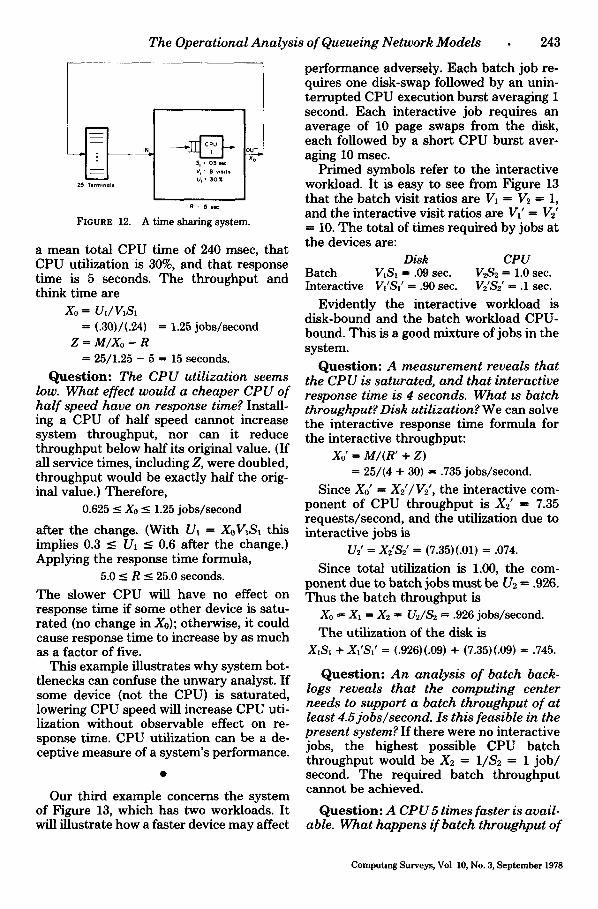
Our second example concerns the 25-ter- minal t ime sharing sys tem of Figure 12. A m e a s u r e m e n t has revealed tha t jobs require
Computmg Surveys, Vol 10, No. 3, September 1978
The Operational Analysis of Queueing Network Models 243
25 Termmall
FIGURE 12.
I loTl I I °-
R = 5 1 1 ¢
A time sharing system.
a mean total CPU t ime of 240 msec, tha t CPU utilization is 30%, and tha t response t ime is 5 seconds. T h e th roughpu t and think t ime are
Xo ffi U,/ V, SI ffi (.30)/(.24) ffi 1.25 j o b s / s e c o n d
Z ffi M/Xo - R ffi 25/1.25 - 5 -- 15 seconds.
Question: The CPU utilization seems low. What effect would a cheaper CPU of hal f speed have on response time? Install- ing a CPU of half speed cannot increase sys tem throughput , nor can it reduce th roughpu t below half its original value. (If all service times, including Z, were doubled, th roughput would be exactly half the orig- inal value.) Therefore ,
0.625 _< Xo ~ 1.25 jobs/second
af ter the change. (With U~ = XoVIS~ this implies 0.3 _< /31 -< 0.6 af ter the change.) Applying the response t ime formula,
5.0 _ R _< 25.0 seconds.
T h e slower CPU will have no effect on response t ime if some other device is satu- ra ted (no change in Xo); otherwise, it could cause response t ime to increase by as much as a factor of five.
Th is example i l lustrates why sys tem bot- t lenecks can confuse the unwary analyst. I f some device (not the CPU) is sa turated, lowering CPU speed will increase CPU uti- lization without observable effect on re- sponse time. CPU utilization can be a de- ceptive measure of a sys tem's performance.
Our third example concerns the sys tem of Figure 13, which has two workloads. I t will i l lustrate how a faster device m a y affect
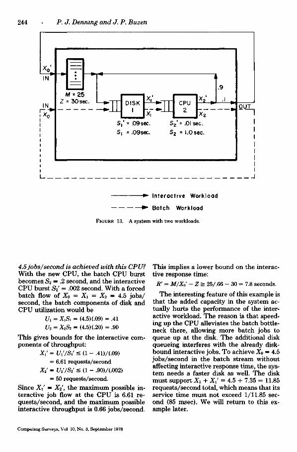
pe r formance adversely. Each ba tch job re- quires one disk-swap followed by an unin- t e r rup ted CPU execution burs t averaging 1 second. Each interact ive job requires an average of 10 page swaps f rom the disk, each followed by a shor t C P U burs t aver- aging 10 msec.
Pr imed symbols refer to the interact ive workload. I t is easy to see f rom Figure 13 t ha t the ba tch visit rat ios are V, ffi 112 = 1, and the interact ive visit rat ios are Vf ffi V2' ffi 10. T h e tota l of t imes required by jobs a t the devices are:
Disk CPU Batch V~S~ ffi .09 sec. V2S2 ffi 1.0 sec. Interactive V,'S,' ffi .90 sec. V2'$2' ffi .1 sec.
Evident ly the interact ive workload is disk-bound and the ba tch workload CPU- bound. This is a good mixture of jobs in the system.
Question: A measurement reveals that the CPU is saturated, and that interactive response time is 4 seconds. What ~s batch throughput? Disk utilization? We can solve the interact ive response t ime formula for the interact ive throughput :
Xo' ffi M/(R' + Z) ffi 25/(4 + 30) = .735 jobs/second.
Since Xo' = X2'/V2', the interact ive com- ponent of CPU th roughpu t is X2' ffi 7.35 reques ts /second, and the utilization due to interact ive jobs is
U2' ffi X{S2' = (7.35)(.01) ffi .074.
Since total utilization is 1.00, the com- ponen t due to ba t ch jobs m u s t be Us = .926. Thus the ba tch th roughpu t is
Xo = X1 ffi X2 = U2/$2 = .926 jobs/second.
T h e utilization of the disk is X,S~ + X{SI' = (.926)(.09) + (7.35)(.09) ffi .745.
Question: An analysis of batch back- logs reveals that the computing center needs to support a batch throughput of at least 4.S jobs~second. Is this feasible in the present system? I f there were no interact ive jobs, the highest possible C P U ba tch th roughpu t would be X2 = 1/82 = 1 j o b / second. T h e required ba tch th roughpu t cannot be achieved.
Question: A CPU 5 times faster is avail- able. What happens if batch throughput of
Computing Surveys, Vol 10, No. 3, September 1978
244 P. J. D e n n i n g a n d J. P. B u z e n
IN I ~ - . 1, ~ L , .9
M = 2 5 , . ,
IN Z = 30sec. - - I ~ - I T DISK " -cJ -~T l " cPu x2' ~_ .I = ' 2 ;OUT
S=' = . 0 9 s e c . S z ' = .01 sec.
S I = . 0 9 s e c . S z = 1 . 0 s e c .
FIGURE 13.
I n t e r o c h v e Workload
4 ~ B o t c h W o r k l o a d
A system with two workloads.
4 . 5 j o b s ~ s e c o n d is ach i eved w i th th i s CPU? With the new CPU, the ba tch CPU burst becomes $2 ffi .2 second, and the interactive CPU burst $2' = .002 second. With a forced ba tch flow of X0 ffi X1 = X2 = 4.5 jobs / second, the ba tch components of disk and CPU utilization would be
U~ = X~S~ = (4.5)(.09) ffi .41 U2 ffi X2S2 ffi (4.5)(.20) = .90
This gives bounds for the interactive com- ponents of throughput :
Xl' ffi UI'/S~' ~- (1 - .41)/(.09) = 6.61 requests/second
X2' = U2'/$2' <- (1 - .90)/(.002) = 50 requests/second.
Since XI' = X2', the maximum possible in- teract ive job flow at the CPU is 6.61 re- quests /second, and the maximum possible interact ive th roughput is 0.66 jobs/second.
This implies a lower bound on the interac- tive response time:
R' = M/Xo' - Z ~_ 25/.66 - 3 0 = 7.8 seconds.
T h e interesting feature of this example is tha t the added capaci ty in the system ac- tually hur ts the performance of the inter- active workload. T h e reason is tha t speed- ing up the CPU alleviates the ba tch bottle- neck there, allowing more ba tch jobs to queue up at the disk. Th e additional disk queueing interferes with the already disk- bound interact ive jobs. To achieve Xo = 4.5 jobs / second in the ba tch s t ream wi thout affecting interact ive response time, the sys- t em needs a faster disk as well. T h e disk must suppor t X1 + XI' ffi 4.5 + 7.35 = 11.85 reques ts / second total, which means tha t its service t ime must not exceed 1/11.85 sec- ond (85 msec). We will re turn to this ex- ample later.
Computmg Surveys, Vol 10, No. 3, September 1978
The Operational Analysis of Queueing Network Models 245
Summary
By augmenting the basic operational defi- nitions with the assumption that job flow is balanced in the system, the analyst can use visit ratios, via the forced flow law, to de- termine flows everywhere in the network. Response times of interactive systems can also be estimated. Table I summarized the principal equations.
When the available information is insuf- ficient to determine flows in the network at a given load, the analyst can still approxi- mate the behavior under light and heavy loads. For light loads the lack of queueing permits determining response time and throughput directly from the products V~S,. For heavy loads, a saturating device limits the flow at one point in the network, thereby limiting the flows everywhere; again, response time and throughput can be computed easily. For intermediate loads, further assumptions about the system are needed.
5. LOAD DEPENDENT BEHAVIOR
The examples of the preceding section were based on assumptions of invariance for ser- vice times, visit ratios, and routing frequen- cies. These assumptions are too rigid for many real systems. For example, if the mov- ing-arm disk employs a scheduler that min- imizes arm movement, a measurement of the mean seek time during a lightly loaded baseline period will differ significantly from the average seek time observed in a heavily loaded projection period. Similarly, the visit ratios for a swapping device will differ in baseline and projection periods having different average levels of multiprogram- ming.
These two examples illustrate load de- pendent behavior. To cope with it, the an- alyst replaces the simple invariance as- sumptions with conditional invariance as- sumptions that express the dependence of important parameters on the load. Instead of asserting that the disk's mean seek time is invariant in all observation periods, the analyst asserts that the mean seek time is the same in any two intervals in which the disk's queue length is the same. That is, the average seek time, whenever the disk's
queue length is n (for any integer n), is assumed to be the same in both the baseline and the projection period, but the propor- tion of time that the queue length is n may differ in the two periods. Similarly, the swapping device's visit ratio whenever the multiprogramming level is N is assumed to be the same in both the baseline and the projection period, but the proportion of time that the multiprogramming level is N may differ in the two periods.
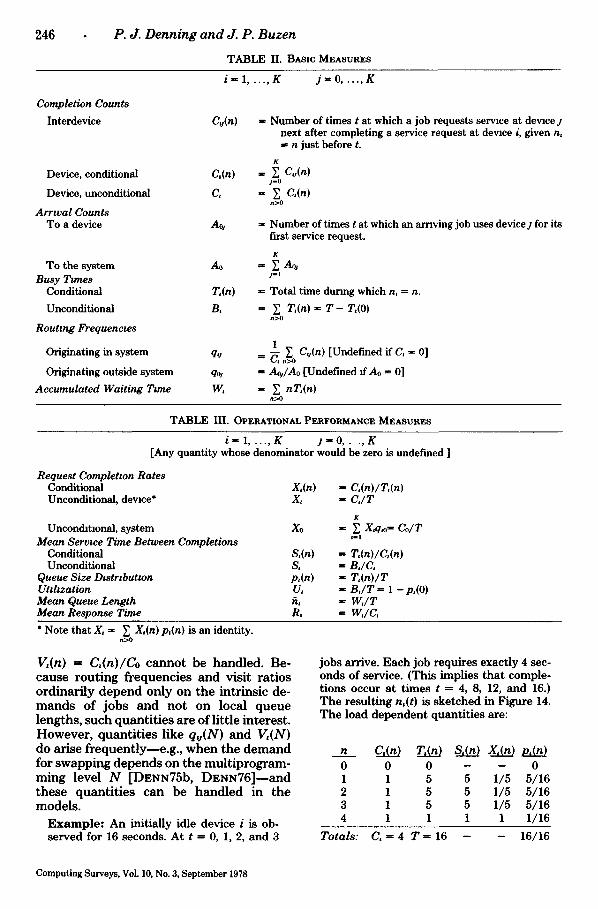
Tables II and III summarize the opera- tional concepts needed to express condi- tional invariants and to work with load dependent behavior. Table II shows that each of the basic quantities (C,j, B,) is re- placed with a function of the load. Thus C,j(n) counts the number of times t at which jobs request service at devicej immediately on completing a service request at device i, given that n, ffi n just before each such time t. The function T,(n) specifies the total time during which n, ffi n.
Table III shows the various operational measures which can be derived from the basic quantities of Table II. There are two new concepts here. The first is the service function, S~(n) ffi 1/X,(n), which measures the mean time between completions when n, = n; if device i can process several service requests at once, S,(n) can be less than the mean amount of service required by a re- quest. The second concept is the queue length distribution, p,(n), which measures the proportion of time during which n, ffi n. That the mean queue length f~, ffi W,/T is equivalent to the usual definition E,>o np,(n) can be seen from the definition of W, in Table II.
The method of partitioning the data ac- cording to time intervals in which n,(t) = n is called stratified sampling. The sets of intervals in which n,(t) ffi n are called the "strata" of the sample. All data in the same stratum are aggregated to form the mea- sures of Tables II and III.
Our analytic methods can deal with only two kinds of load dependent behavior: a device's service function may depend on the length of that device's queue; the visit ratios and routing frequencies may depend on the total number of jobs in the system. Thus quantities like q,~(n) = C~(n)/C,(n) or
Computing Surveys. Vol. 10, No. 3, September 1978
246 P . J . D e n n i n g a n d J . P . B u z e n
TABLE II. BASXC MEASURES
Completion Counts
Interdevice
Device, conditional
Device, unconditional
Arrwal Counts To a device
To the system Busy Ttmes
Conditional
Unconditional
Routing Frequencws
Originating in system
Originating outside system
Accumulated Waiting Ttme
iffi l . . . . . K jffi0 . . . . . K
C,j(n)
C,(n)
C,
Ao~
Ao
T,(n)
B,
qv
qo~
W,
ffi Number of times t at which a job requests service at device j next after completing a service request at devlce i, given n, s n just before t.
K
= ~ C.j(n) j-o
ffi ~ C,(n) n>0
ffi Number of times t at which an arrwing job uses devicej for its first service request.
E
== ~ A o j j l l
ffi Total time dunng which n, ffi n.
= ~ T,(n) = T - T,(0) n>0
1 ~ C,j(n) [Undefined if C, ffi 0] --~ C , n > O
ffi AoJAo [Undefined ff Ao -- 0]
= ~ nT,(n) n:>O
TABLE Ill. OPERATIONAL PERFORMANCE MEASURES
i ff i l . . . . . K yffi0 . . . . K [Any quantity whose denominator would be zero is undefined ]
Request Completton Rates Conditional X,(n) ffi C,(n)/T,(n) Unconditional, dewce* X, - C J T
K
Unconchtlonal, system Xo = ~. X,q,0ffi ColT #--l Mean Service Time Between Completions
Conditional S,(n) ffi T,(n)/C,(n) Unconditional S, ffi B,/C,
Queue Size Dtstrtbutwn p,(n) ffi T,(n)/T Utthzation U, ffi B , / T ffi 1 -p,(O) Mean Queue Length fz, ffi W , / T Mean Response Time R, ffi W,/C,
* Note that X, ffi ~ X,(n) p,(n) is an identity. n>0
V,(n) ffi C , ( n ) l C o c a n n o t be hand led . Be- cause r o u t i n g f requenc ies a n d visi t ra t ios o rd ina r i l y d e p e n d on ly on t he in t r ins ic de- m a n d s of jobs a n d n o t on local queue lengths , such q u a n t i t i e s are of l i t t le in te res t . However , q u a n t i t i e s l ike q v ( N ) a n d V , ( N ) do arise f r equen t ly - - e . g . , w h e n the d e m a n d for swapp ing d e p e n d s o n the m u l t i p r o g r a m - m i n g level N [DE~N75b, D E s ~ 7 6 ] - - a n d these q u a n t i t i e s c an be h a n d l e d in the models .
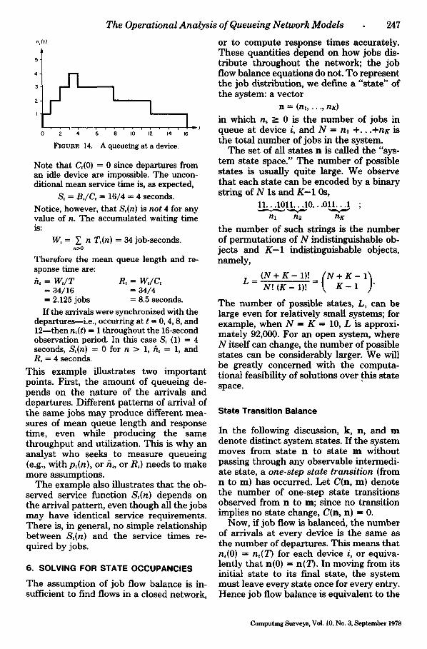
E x a m p l e : An initially idle device i is ob- served for 16 seconds. At t -- 0, 1, 2, and 3
jobs arrive. Each job requires exactly 4 sec- onds of service. (This implies that comple- tions occur at times t -- 4, 8, 12, and 16.) The resulting n,(t) is sketched in Figure 14. The load dependent quantities are:
n C,(n) T,(n) Sf(n) Xf(n) p,(n)
0 0 0 - - 0 1 1 5 5 1/5 5/16 2 1 5 5 1/5 5/16 3 1 5 5 1/5 5/16 4 1 1 1 1 1/16
Totals: C, ffi4 T ffi 16 - - 16/16
Computing Surveys, Vol. 10, No. 3, September 1978
n, f t )
5
3
2 ¸
2 4 6
FIGURE 14.
T h e O p e r a t i o n a l A n a l y s i s o f Q u e u e i n g N e t w o r k M o d e l s • 247
I I
I 8 I0 12 14 16
A queueing at a device.
Note that C,(0) = 0 since departures from an idle device are impossible. The uncon- ditional mean service time is, as expected,
S, ffi B,/C, ffi 16/4 = 4 seconds.
Notice, however, that S,(n) is not 4 for any value of n. The accumulated waiting time is:
W, = Y. n T,(n) = 34 job-seconds. n > 0
Therefore the mean queue length and re- sponse time are: ~, = W , / T R, = W , / C ,
= 34/16 = 34/4 -- 2.125 jobs = 8.5 seconds. If the arrivals were synchronized with the
departuresmi.e., occurring at t = 0, 4, 8, and 12--then n,(t) = I throughout the 16-second observation period. In this case S, (1) = 4 seconds, S,(n) = 0 for n > 1, f~, = 1, and R, = 4 seconds.
This example illustrates two impor tant points. First, the amount of queueing de- pends on the nature of the arrivals and departures. Different pat terns of arrival of the same jobs may produce different mea- sures of mean queue length and response time, even while producing the same throughput and utilization. This is why an analyst who seeks to measure queueing (e.g., wi thp,(n) , or fz,, or R,) needs to make more assumptions.
T he example also illustrates tha t the ob- served service function S,(n) depends on the arrival pat tern, even though all the jobs may have identical service requirements. There is, in general, no simple relationship between S,(n) and the service times re- quired by jobs.
6. SOLVING FOR STATE OCCUPANCIES
T he assumption of job flow balance is in- sufficient to find flows in a closed network,
or to compute response t imes accurately. These quantit ies depend on how jobs dis- t r ibute throughout the network; the job flow balance equations do not. To represent the job distribution, we define a "s ta te" of the system: a vector
n - - ( n l , . . . . nx)
in which n, __ 0 is the number of jobs in queue at device i, and N = n~ + . . . + n K is the total number of jobs in the system.
The set of all s tates n is called the "sys- t em state space." Th e number of possible states is usually quite large. We observe tha t each state can be encoded by a binary string of N ls and K - 1 0s,
11...1011...10...011...1 ;
nl n2 nK
the number of such strings is the number of permutat ions of N indistinguishable ob- jects and K - 1 indistinguishable objects, namely,
L f ( N + K - 1 ) ! [ N + K - 1 ) N ! ( K - 1 ) ! = ~ K - 1 _"
T h e number of possible states, L, can be large even for relatively small systems; for example, when N ffi K = 10, L is approxi- mately 92,000. For an open system, where N itself can change, the number of possible states can be considerably larger. We will be greatly concerned with the computa- tional feasibility of solutions over this state space.
State Transition Balance
In the following discussion, k, n, and m denote distinct system states. If the system moves from state n to s tate m without passing through any observable intermedi- ate state, a one-s tep s ta te t rans i t ion (from n to m) has occurred. Let C(n, m) denote the number of one-step state transitions observed from n to m; since no transition implies no state change, C(n, n) = 0.
Now, if job flow is balanced, the number of arrivals at every device is the same as the number of departures. This means tha t n~(0) = n,(T) for each device i, or equiva- lently tha t n(0) ffi n(T). In moving from its initial state to its final state, the system must leave every state once for every entry. Hence job flow balance is equivalent to the
Computing Surveys, Vol. 10, No. 3, September 1978

248 P. J. Denning and J. P. Buzen
Principle of State Transition Balance: The number of entries to every state is the same as the number of exits from that state during the observation period.
From now on we will use the term flow balance to mean that arrivals equal depar- tures at every device or system state. With the flow balance principle we can write "conservation of transition" equations:
C(k,n) ffi~C(n,m) all n. k m
For given n, both sides of this equation are 0 if and only if T(n) = 0.
If we use these equations without flow balance, the only error would be a + 1 (or -1) term missing on the right side if n is the final (or initial) state of the system for the observation period. This error is not significant if the initial and final states are visited frequently during the observation period. (The error is zero if the initial and final states are the same--i.e., flow is bal- anced.) As we noted in discussing job flow balance, choosing the observation period so that flow is balanced is not a new notion.
The "transition rate" from n to m is the number of transitions per unit time while n is occupied:
r (n , m ) ffi C(n , m ) / T ( n ) ;
it is not defined if T(n) ffi 0. The transition conservation equations can be re-expressed a s
Y. T(k) r(k, n) -- T(n) ~ r(n, m), k m
for all n from which exit rates r(n, m) are defined; note T(n) ffi 0 if r(n, m) is not defined. Substituting T(n) -- p(n)T and cancelling T, we obtain the
STATE SPACE BALANCE EQUATIONS
p(k) r(k, n) = p(n) ~ r(n, m) k m
for all n in which r(n,.) is defined.
Because the T(n) sum to T, we can aug- ment these equations with the normalizing condition
p(n) = 1. n
If the system can move from any n to any m, then these are L - 1 linearly independent balance equations; only one set ofp(n) can satisfy them and the normalizing condition
simultaneously. (Our definitions imply p(n) = 0 for states not included in these balance equations.)
Solving the Balance Equations
The state space balance equations are op- erational relationships expressing the val- ues of p(n) in terms of the r(n, m). This form of expression is generally not useful since the analyst does not have the values of r(n, m). Instead, the analyst wishes to express the r(n, m) in terms of available quantities such as visit ratios and the ser- vice functions, and then solve for the p(n).
To avoid a lot of symbol manipulation, we will outline the steps of the solution; the details are found in [DENN77a]. The solu- tion uses two additional assumptions about system's behavior. The first is:
One-Step Behavior: The only observ- able state changes result from single jobs either entering the system, or mov- ing between pairs of devices in the sys- tem, or exiting from the system.
The hypothesis of one-step behavior asserts that simultaneous job-moves will not be observed; it reduces the number of nonzero rates r(n, m) that must be considered. For example, when a job moves from device i to device j, the system moves from state n to its "neighbor," n,j, where
n = (nl , , n,, , nj, , nK) n,~ffi ( n l , . . , n , - 1 , . . , n j + 1, ,nK) .
The nonzero transition rates correspond to (i, j ) job moves under the one-step assump- tion. Thus there are about LK "~ rates to specify, rather than L e. (L is the size of the state space.) With this assumption, r(n, n,j) depends only on the rate of job flow from device i to device j. The one-step property is met in many real systems.
To specify the transition rates in terms of routing frequencies and service func- tions, we need to remove the conditioning on the total system state. The assumptions that do this are called "homogeneity" be- cause they assert that, for given n,, device i is influenced equally by all system states:
Devtce Homogeneity: The output rate of a device is determined completely by its queue length, and is otherwise indepen- dent of the system's state.
Computing Surveys, Vo|. 10, No. 3, September 1978
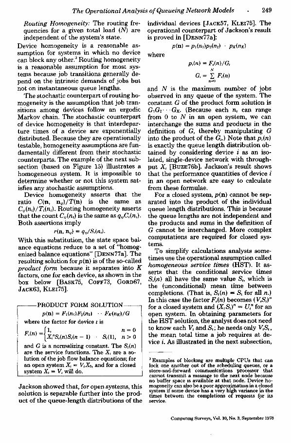
The Operational Analys i s of Queueing Network Mode ls 249
Rout ing Homogeneity: The routing fre- quencies for a given total load (N) are independent of the system's state.
Device homogeneity is a reasonable as- sumption for systems in which no device can block any other. 3 Routing homogeneity is a reasonable assumption for most sys- tems because job transitions generally de- pend on the intrinsic demands of jobs but not on instantaneous queue lengths.
The stochastic counterpart of routing ho- mogeneity is the assumption that job tran- sitions among devices follow an ergodic Markov chain. The stochastic counterpart of device homogeneity is that interdepar- ture times of a device are exponentially distributed. Because they are operationally testable, homogeneity assumptions are fun- damentally different from their stochastic counterparts. The example of the next sub- section (based on Figure 15) illustrates a homogeneous system. It is impossible to determine whether or not this system sat- isfies any stochastic assumptions.
Device homogeneity asserts that the ratio C(n, n~j)/T(n) is the same as C,~(nJ/T~(n,). Routing homogeneity asserts that the count Cu(nt) is the same as q,jCt(n,). Both assertions imply
r(n, n,~) = qJS~(n,).
With this substitution, the state space bal- ance equations reduce to a set of "homog- enized balance equations" [DENN77a]. The resulting solution forp(n) is of the so-called product form because it separates into K factors, one for each device, as shown in the box below [BASK75, COFF73, GORD67, JACK63, KLEI75].
-.PRODUCT FORM SOLUTION p(n) = F~(n~)F2(n2) .. Fg(ng)/G
where the factor for device t is I1, n -- 0
F,(n) ~- X~S,(n)S,(n _ 1) S,(1), n > 0
and G is a normalizing constant. The S~(n) are the service functions. The X, are a so- lution of the job flow balance equations; for an open system X~ = V, Xo, and for a closed system X~ ffi IT, will do.
Jackson showed that, for open systems, this solution is separable further into the prod- uct of the queue-length distributions of the
individual devices [JACK57, KLEI75]. The operational counterpart of Jackson's result is proved in [DENN77a]:
p(n) =pl(nl)p2(n2) " pK(n~)
where p,(n) = F,(n)/G,
N
G, ffi ~ F,(n) n~O
and N is the maximum number of jobs observed in any queue of the system. The constant G of the product form solution is GIG2"" "GK. (Because each n, can range from 0 to N in an open system, we can interchange the sums and products in the definition of G, thereby manipulating G into the product of the G,.) Note that pt(n) is exactly the queue length distribution ob- tained by considering device i as an iso- lated, single-device network with through- put Xt [BvzE76b]. Jackson's result shows that the performance quantities of device i in an open network are easy to calculate from these formulae.
For a closed system, p(n) cannot be sep- arated into the product of the individual queue length distributions. This is because the queue lengths are not independent and the products and sums in the definition of G cannot be interchanged. More complex computations are required for closed sys- tems.
To simplify calculations analysts some- times use the operational assumption called homogeneous service times (HST). It as- serts that the conditional service times St(n) all have the same value St, which is the (unconditional) mean time between completions. (That is, St(n) = St for all n.) In this case the factor F,(n) becomes ( V, St) n for a closed system and (XtS,) n ffi U, n for an open system. In obtaining parameters for the HST solution, the analyst does not need to know each V, and St; he needs only VtSt, the mean total time a job requires at de- vice i. As illustrated in the next subsection,
3 Examples of blockmg are mul t ip le C P U s tha t can lock one ano the r ou t of the schedul ing queues , or a s tore-and-forward communica t ions processor t ha t canno t t r ansmi t a message to t he nex t node because no buffer space is available a t t ha t node. Device ho- mogene i ty can also be a poor app rox imahon in a closed sy s t em if some device h a s a very h igh var iance in t he t imes be tween the comple t ions of reques t s for i ts service.
Computing Surveys. VoL 10, No. 3, September 1978
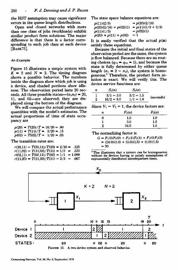
250 P. J. Denning and J. P. Buzen
the H S T assumption may cause significant errors in the queue length distributions.
Open and closed networks with more than one class of jobs (workloads) exhibit similar product form solutions. The major difference is tha t there is a factor corre- sponding to each job class at each device [BASK75].
An Example
Figure 15 illustrates a simple system with K ffi 2 and N -- 2. The timing diagram shows a possible behavior. The numbers inside the diagram show which job is using a device, and shaded portions show idle- ness. The observation period lasts 20 sec- onds. All three possible states--(nln2) ffi 20, 11, and 02--are observed; they are dis- played along the bot tom of the diagram.
We will compare the actual performance quantities with the model 's estimates. The actual proport ions of time of state occu- pancy are
p(20) ffi T(20)/T ffi 16/20 = .80 p(11) ffi T(11)/T-- 3/20--.15 p(02) -- T(O2)/T = 1/20 = .05
The transition rates are:
r(20,11) ffi T(20,11)/T(20) = 2/16 = .125 r(11,02) ffi T(11,02)/T(11) = 1/3 -- .333 r(02,11) ffi T(O2,11)/T(02) ffi 1/1 ffi 1.000 r(11,20) ffi T(ll,20)/T(11) ffi 2/3 = .667
The state space balance equations are: p(11)(2/3) ffi p(20)(2/16) p(20)(2/16) + p(02)(1) = p(11)(1/3 + 2/3) p(11)(1/3) = p(02)(1) p(20) +p(11) +p(02) = 1
I t is easily verified that the actual p(n) satisfy these equations.
Because the initial and final states of the observation period are the same, the system is flow balanced. Because there are no rout- ing choices (q12 = q21 = 1) , and because the state is fully determined by either queue length (nl ffi 2 - n 2 ) , the system is homo- geneous. 4 Therefore, the product form so- lution is exact. We will verify this. The device service functions are:
n St(n) S~(n)
1 3/1 = 3.0 3/2 = 1.5 (seconds) 2 16/2 = 8.0 1/1 = 1.0
Since I11 ffi V2 ffi 1, the device factors are:
n Fl(n) F~(n)
0 1.0 1.0 1 3 . 0 1 .5
2 24.0 1.5
The normalizing factor is G -- F](2)F2(0) + F](1)F2(1) + F](0)F2(2)
: (24.0)(1.0) + (3.0)(1.5) + (1.0)(1.5) : 30
(This illustrates that a system can be homogeneous without its devices having to satisfy assumphons of exponentially distributed mterdeparture times.
×o .el
Device I
Device 2
STATES :
K = 2 N = 2
T 0 I0 II 12 13 19 2 0
I I I I I I I i i ~ / j i . • i i i i
I 2 ~ / I 2 ,
20 II 02 II 20 II 20 FIGURE 15. A two-device system and observed behavior.
Computing Surveys, Vol. 10, No. 3, September 1978
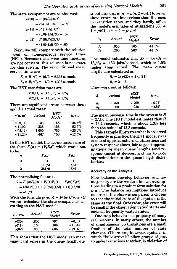
The Operat ional Analys is o f Queueing Ne twork Mode l s
T h e s ta te occupancies are as observed: p(20) -- F~(2)F2(O)/G
-- (24.0)(1.0)/30--.80 p(11) -- F~(1)F2(1)/G
= (3.0)(1.5)/30 = .15
p(02) -- FI(O)F2(2)/G
ffi (1.0)(1.5)/30 = .05
Next, we will compare with the solution based on homogeneous service t imes (HST). Because the service t ime functions are not constant, this solution is not exact for this system. T h e uncondit ional mean service t imes are
$1 = B1/C1 ffi 19/3 = 6.333 seconds
$2 = B2/C2 = 4/3 = 1.333 seconds
T h e H S T transi t ion ra tes are r(20,11) = r(11,02) ffi 1/$1
r(02,11) ffi r(11,20) = 1/$2
There are significant errors be tween these and the actual rates:
HST r(n, m) Actual Model Error
r(20,11) .125 . 1 5 8 +26.4% r(ll,02) .333 .158 -52.5% r(02,11) 1.000 .750 -25.0% r(ll,20) .667 .750 +12.5%
In the H S T model, the device factors are of the form F,(n) ffi (V, S J n, which works out to be:
n Fdn) F2(n)
0 1 1 1 19/3 4/3 2 361/9 16/9
T h e normalizing factor is G -- Fl(2)F2(0) + Fz(1)F2(1) + F~(0)F2(2)
= (361/9)(1) + (19/3)(4/3) + (1)(16/9) ffi 453/9
With the formula p(nln2) = FI(n])F2(n2)/G we can calculate the s ta te occupancies ac- cording to the H S T model:
HST p(n]n2) Actual Model Error
p(20) .800 .797 -0.4% p( l l ) .150 .168 +11.8% p(02) .050 .035 -29.3%
This shows tha t the H S T model can make significant errors in the queue length dis-
251
tr ibutions, e.g.,p](n) = p(n, 2 - n). However these errors are less serious than the ones in t ransi t ion rates, and they hardly affect the model ' s es t imates of utilizations (U] = 1 - p ( 0 2 ) , /-?2 = 1 - p ( 2 0 ) ) :
HST Error U~ Actual Model
U1 .950 .965 +1.5% U2 .200 .203 +1.5%
T h e model es t imates tha t X0 ffi U1/S1 ffi U2/$2 ffi .152 jobs /second, which is 1.5% higher t han actual. T h e m e a n queue lengths are calculated as
f~l ffi 2.p(20) + 1 .p( l l )
h2 = 2 - fil
T h e y work out as follows:
l IST Error fz, Actual Model
ft~ 1.750 1.762 +0.7% h2 .250 .238 -4.8%
T h e m e a n response t ime in the sys tem is R = 2/Xo. T h e H S T model es t imates t ha t R = 13.2 seconds, which is abou t 1.3% less t han the actual of 13.3 seconds.
This example i l lustrates wha t is observed f requent ly in practice: the H S T model gives excellent approximat ions of utilizations and sys tem response times, fair to good approx- imat ions for m e a n queue lengths (and re- sponse times) a t devices; and fair to poor approximat ions to the queue length distri- butions.
Accuracy of the Analysis
Flow balance, one-step behavior , and ho- mogene i ty are the weakes t known assump- t ions leading to a p roduc t fo rm solution for p (n) . T h e balance assumpt ions introduce no error if the observat ion period is chosen so t ha t the initial s ta te of the sys t em is the same as the final. Otherwise, the error will be small if the observat ion per iod s tar ts and ends on f requent ly visited states.
One-s tep behav ior is a p roper ty of m a n y real systems. In m a n y others, the n u m b e r of s imul taneous job t ransi t ions are a small fract ion of the total n u m b e r of s ta te changes. (There are, however, sys tems in which "bulk arr ivals" allow groups of jobs to make t ransi t ions together , in violation of
t
Computing Surveys, Vol. 10, No. 3, September 1978
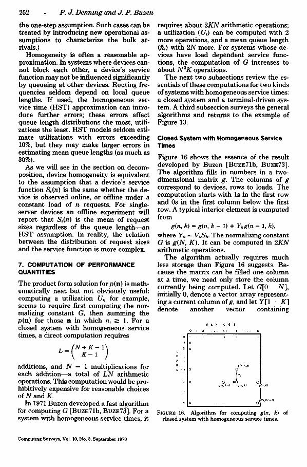
252 P. J. Denning a n d J. P. Buzen
the one-step assumption. Such cases can be treated by introducing new operational as- sumptions to characterize the bulk ar- rivals.)
Homogeneity is often a reasonable ap- proximation. In systems where devices can- not block each other, a device's service function may not be influenced significantly by queueing at other devices. Routing fre- quencies seldom depend on local queue lengths. If used, the homogeneous ser- vice time (HST) approximation can intro- duce further errors; these errors affect queue length distributions the most, utili- zations the least. HST models seldom esti- mate utilizations with errors exceeding 10%, but they may make larger errors in estimating mean queue lengths (as much as 30%).
As we will see in the section on decom- position, device homogeneity is equivalent to the assumption that a device's service function S,(n) is the same whether the de- vice is observed online, or offline under a constant load of n requests. For single- server devices an offiine experiment will report that S,(n) is the mean of request sizes regardless of the queue length--an HST assumption. In reality, the relation between the distribution of request sizes and the service function is more complex.
7. COMPUTATION OF PERFORMANCE QUANTITIES
The product form solution forp(n) is math- ematically neat but not obviously useful: computing a utilization U,, for example, seems to require first computing the nor- malizing constant G, then summing the p(n) for those n in which n, _ 1. For a closed system with homogeneous service times, a direct computation requires
[ N + K - 1) L---~ K - 1
additions, and N - 1 multiplications for each addition--a total of L N arithmetic operations. This computation would be pro- hibitively expensive for reasonable choices of N and K.
In 1971 Buzen developed a fast algorithm for computing G [BuzE71b, B~ZE73]. For a system with homogeneous service times, it
requires about 2 K N arithmetic operations; a utilization (U,) can be computed with 2 more operations, and a mean queue length (fz,) with 2N more. For systems whose de- vices have load dependent service func- tions, the computation of G increases to about N 2 K operations.
The next two subsections review the es- sentials of these computations for two kinds of systems with homogeneous service times: a closed system and a terminal-driven sys- tem. A third subsection surveys the general algorithms and returns to the example of Figure 13.
Closed System with Homogeneous Service Times
Figure 16 shows the essence of the result developed by Buzen [Buzz71b, BUZE73]. The algorithm fills in numbers in a two- dimensional matrix g. The columns of g correspond to devices, rows to loads. The computation starts with ls in the first row and 0s in the first column below the first row. A typical interior element is ,computed from
g(n, k) ffi g(n, k - 1) + Ykg(n - 1, k),
where Yk ffi VkSk. The normalizing constant G is g(N, K) . It can be computed in 2KN arithmetic operations.
The algorithm actually requires much less storage than Figure 16 suggests. Be- cause the matrix can be filled one column at a time, we need only store the column currently being computed. Let G[0 N], initially 0, denote a vector array represent- ing a current column of g, and let Y[1 K] denote another vector containing
O E V I C E S
0 t 2 ... k-t k ... K
, 0 . . . . ii 0
A
O o(n-i, k) $ n-t .~¥,
n C fl(n. k - I I ¢(n. k) g(n,K)
• I O(N,K) • G
N o I
FmURE 16. Algorithm for computing g(n, k) of closed system with homogeneous servme times.
Computing Surveys, Vol. 10, No. 3, September 1978
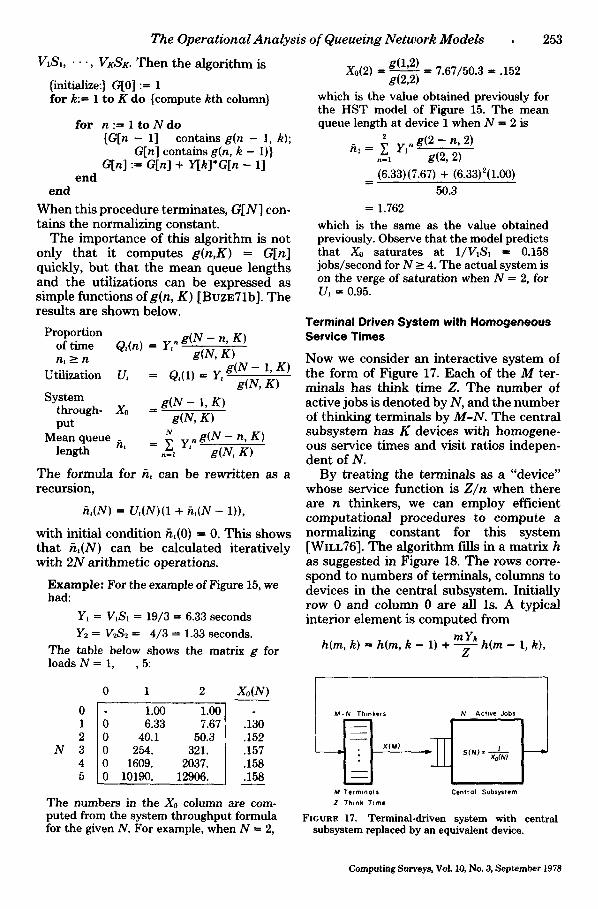
T h e O p e r a t i o n a l A n a l y s i s o f Q u e u e i n g N e t w o r k M o d e l s
VIS1, • • -, VKSK. T h e n the a lgor i thm is
(initialize:} G[0] :-- 1 f o r k:= I to K do {compute kth column}
for n : f l t o N d o { G [ n - 1] contains g(n - 1, k);
G[n] c o n t a i n s g(n, k - 1)} G[n] := Gin] + Y[k]*G[n - 1]
e n d e n d
When this procedure terminates , G[N] con- tains the normalizing constant.
T h e impor tance of this a lgor i thm is not only tha t it computes g ( n , K ) = Gin] quickly, but tha t the m e a n queue lengths and the utilizations can be expressed as s imple functions o fg(n , K) [BvzE71b]. T h e results are shown below.
Proportion of time n,>_n
Utilization
System through- Xo put
Mean queue -
Q,(n) = Y," g (N - n, K) g(N, K)
U, = Q,(1) = Y, g ( N - 1, K) g iN, K)
= g (N - 1, K) g(N, K)
N length n, = ~ y , , g (N - n, K)
.-z giN, K)
T h e formula for fz, can be rewri t ten as a recursion,
fi,(N) = U,(N)(1 + f~,iN - 1)),
wi th in i t ia l condit ion f~,(O) = O. Th is shows that f~,(N) can be calculated i te ra t ive ly with 2N ar i thmet ic operations.
Example : For the example of Figure 15, we had:
Y~ = VIS1 = 19/3 = 6.33 seconds Y2 = V2S2 = 4/3 = 1.33 seconds.
The table below shows the matrix g for loads N = 1, ,5:
N
0
0 1 0 2 0 3 0 4 0 5 0
1 2 Xo(N)
1.00 1.00 I 6.33 7.67 .130
40.1 50.3 I .152 254. 321. 1 . 1 5 7
1609. 2037. .158 10190. 12906. .158
The numbers in the Xo column are com- puted from the system throughput formula for the given N. For example, when N = 2,
253
g(1,2) X0(2) = - - = 7.67/50.3 = .152
g(2,2) which is the value obtained previously for the HST model of Figure 15. The mean queue length at device 1 when N = 2 is
2
ftl = ~. Y1 n g(2 - n, 2) .-1 g(2, 2) (6.33)(7.67) + (6.33)2(1.00)
50.3
= 1.762 which is the same as the value obtained previously. Observe that the model predicts that X0 saturates at 1/V1S1 = 0.158 jobs/second for N ~ 4. The actual system is on the verge of saturation when N = 2, for U1 = 0.95.
Terminal Driven System with Homogeneous Service Times
Now we consider an i n te rac t i ve system of the fo rm of Figure 17. Each of the M ter- minals has think t ime Z. T h e n u m b e r of act ive jobs is denoted by N, and the number of thinking terminals by M - N . T h e central subsys tem has K devices with homogene- ous service t imes and visit rat ios indepen- dent of N.
By t reat ing the terminals as a "device" whose service function is Z / n when there are n thinkers, we can employ efficient computa t iona l procedures to compute a normalizing cons tant for this sys tem [WILL76]. T h e a lgor i thm fills in a mat r ix h as suggested in Figure 18. T h e rows corre- spond to number s of terminals , columns to devices in the central subsystem. Init ially row 0 and column 0 are all ls. A typical interior e lement is computed f rom
m Y , h(m, k) = h(m, k - 1) + T h i m - 1, k),
I M - N Thinkers N Active Jobs /
1 M Termmaq$ Centrol Subsystem
Z Th~nk T~me
FmURE 17. Termina l -dr iven s y s t e m wi th central s u b s y s t e m replaced by an equiva lent device.
Computing Surveys, Vol. 10, No. 3, September 1978
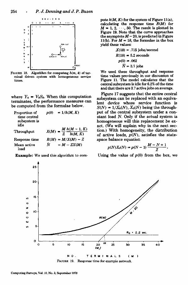
254 P. J. Denning a n d J. P. B u z e n
0 t 2
0 I I
N I 0
2
T : E R
M I
N m &
L
S
t~
D E V I C E S
* . , ~-f It • . . K
n(M,K) 0
FIGURE 18. Algorithm for computing h(m, k) of ter- minal driven system with homogeneous service times.
where Yk = VkSk. When this computa t ion terminates , the per formance measures can be compu ted f rom the formulae below.
Proportion of p(0) ffi 1/h(M, K) time central subsystem is idle
M h ( M - 1, K) Throughput X(M) ffi
Z h(M, K)
Response time R(M) = M/X(M) - Z Mean active fV ffi M - ZX(M)
load
Example : We used this algorithm to corn-
pute h(M, K) for the system of Figure 11(a), calculating the response time R(M) for M = 1, 2, . - - , 50. The result is plotted in Figure 19. Note that the curve approaches the asymptote M - 20, is predicted in Figure 11(b). For M ffi 18, the formulae in the box yield these values:
X(18) = .715 jobs/second R(18) = 5.2 seconds
p(0) = .062 N = 3.7 jobs
We used these throughput and response time values previously in our discussion of Figure 11. The model calculates that the central subsystem is idle for 6.2% of the time and that there are 3.7 active jobs on average.
Figure 17 suggests tha t the ent i re central subsys t em can be replaced with an equiva- lent device whose service function is S ( N ) = 1/Xo(N), Xo(N) being the through- pu t of the centra l subsys tem under a con- s t an t load N. Only if the actual sys tem is homogeneous will this r ep lacement be ex- act. (We will explain why in the next sec- tion.) Wi th homogenei ty , the distr ibution of act ive loads, p ( N ) , satisfies the s ta te- space balance equat ion
- N + I P ( N ) X ° ( N ) = p ( N - 1 ) M Z
Using the value of p(0) f rom the box, we
(n
o
z
o
(.3
tJJ
(n
J
25"
20-
IO
0 0 IO I,~ 2 0 Z2 ~ 3 0 3 5 4 0
(M j)
N O . T E R M I N A L S ( M
FIGURE 19. Response time for example network.
Computing Surveys, Vol. 10, No. 3, September 1978
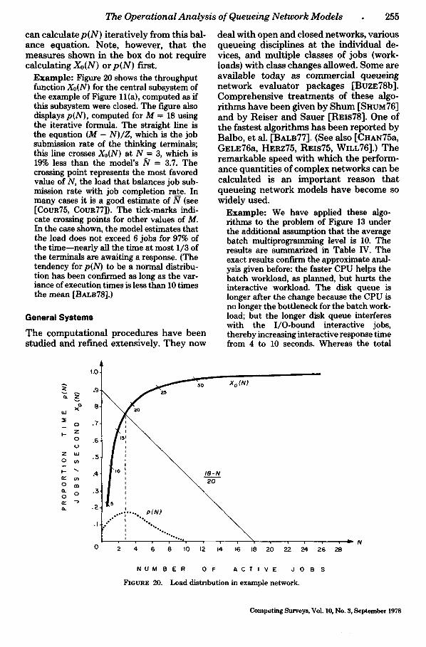
The Operational Analysis of Queueing Network Models 255
can calculate p(N) iteratively from this bal- ance equation. Note, however, that the measures shown in the box do not require calculating Xo(N) orp (N) first.
Example: Figure 20 shows the throughput function Xo(N) for the central subsystem of the example of Figure 11(a), computed as if this subsystem were closed. The figure also displays p(N), computed for M = 18 using the iterative formula. The straight line is the equation (M - N)/Z, which is the job submission rate of the thinking terminals; this line crosses Xo(N) at N = 3, which is 19% less than the model's ,~ ffi 3.7. The crossing point represents the most favored value of N, the load that balances job sub- mission rate with job completion rate. In many cases it is a good estimate of N (see [CouR75, COUR77]). The tick-marks indi- cate crossing points for other values of M. In the case shown, the model estimates that the load does not exceed 6 jobs for 97% of the time--nearly all the time at most 1/3 of the terminals are awaiting a response. (The tendency for p(N) to be a normal distribu- tion has been confirmed as long as the var- iance of execution times is less than 10 times the mean [BALB78].)
General Systems
The computational procedures have been studied and refined extensively. They now
deal with open and closed networks, various queueing disciplines at the individual de- vices, and multiple classes of jobs (work- loads) with class changes allowed. Some are available today as commercial queueing network evaluator packages [BuzE78b]. Comprehensive treatments of these algo- rithms have been given by Shum [SHUM76] and by Reiser and Sauer [Rzxs78]. One of the fastest algorithms has been reported by Balbo, et al. [BALB77]. (See also [CHAN75a, GELE76a, HERZ75, REIS75, WILL76].) The remarkable speed with which the perform- ance quantities of complex networks can be calculated is an important reason that queueing network models have become so widely used.
Example: We have applied these algo- rithms to the problem of Figure 13 under the additional assumption that the average batch multiprogramming level is 10. The results are summarized in Table IV. The exact results confnTn the approximate anal- ysis given before: the faster CPU helps the batch workload, as planned, but hurts the interactive workload. The disk queue is longer after the change because the CPU is no longer the bottleneck for the batch work- load; but the longer disk queue interferes with the I/O-bound interactive jobs, thereby increasing interactive response time from 4 to 10 seconds. Whereas the total
"° t X o (N)
o ~
7-" " .4t I ~ : \ m-N n,. 0 3 o m ' 2 0
o o ~ "" .
N
0 2 4 6 8 I0 12 14 16 18 20 22 24 26 28
N U M B E R O F A C T I V E J O B S
FIGURE 20. Load distribution in example network.
Computing Surveys, Vol. 10, No. 3, September 1978
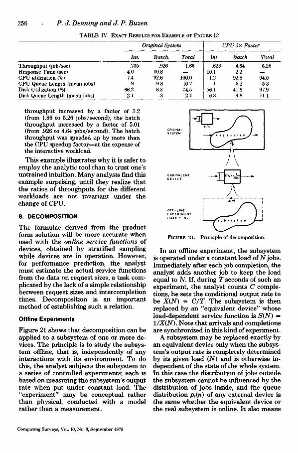
256 P. J. Denning and J. P. Buzen
TABLE IV. EXACT RESULTS FOR EXAMPLE OF FIGURE 13
Throughput (job/sec) Response Time (sec) CPU utihzation (%) CFU Queue Length (mean jobs) Disk Utilization (%) Disk Queue Length (mean jobs)
Ortginal System
Int. Batch. Total
.735 .926 1.66 4.0 10.8 - - 7.4 92.6 100.0
.9 9.8 10.7 66,2 8.3 74.5
2.1 .3 2.4
CPU 5× Faster
Int. Batch Total
.623 4.64 5.26 10.1 2 2 - - 1.2 92.8 94.0
1 5.2 5 3 56.1 41,8 97,9
6.3 4.8 11 1
throughput increased by a factor of 3.2 (from 1.66 to 5.26 jobs/second), the batch throughput increased by a factor of 5.01 (from .926 to 4.64 jobs/second). The batch throughput was speeded up by more than the CPU speedup factor--at the expense of the interactive workload.
This example illustrates why it is safer to employ the analytic tool than to trust one's untrained intuition. Many analysts find this example surprising, until they realize that the ratios of throughputs for the different workloads are not invariant under the change of CPU.
8. DECOMPOSITION
The formulae derived from the product form solution will be more accurate when used with the online service functions of devices, obtained by stratified sampling while devices are in operation. However, for performance prediction, the analyst must estimate the actual service functions from the data on request sizes, a task com- plicated by the lack of a simple relationship between request sizes and intercompletion times. Decomposition is an important method of establishing such a relation.
Offline Experiments
Figure 21 shows that decomposition can be applied to a subsystem of one or more de- vices. The principle is to study the subsys- tem offline, that is, independently of any interactions with its environment. To do this, the analyst subjects the subsystem to a series of controlled experiments; each is based on measuring the subsystem's output rate when put under constant load. The "experiment" may be conceptual rather than physical, conducted with a model rather than a measurement.
ORIGINAL SYSTEM
EQUIVALENT DEVtCE
OFF-LINE EXPERIMENT ( Iood = N )
FIGURE 21. Pnnclple of decomposition.
In an offline experiment, the subsystem is operated under a constant load of N jobs. Immediately after each job completion, the analyst adds another job to keep the load equal to N. If, during T seconds of such an experiment, the analyst counts C comple- tions, he sets the conditional output rate to be X(N) = C/T. The subsystem is then replaced by an "equivalent device" whose load-dependent service function is S(N) ffi 1/X(N). Note that arrivals and completions are synchronized in this kind of experiment.
A subsystem may be replaced exactly by an equivalent device only when the subsys- tem's output rate is completely determined by its given load (N) and is otherwise in- dependent of the state of the whole system. In this case the distribution of jobs outside the subsystem cannot be influenced by the distribution of jobs inside, and the queue distribution p,(n) of any external device is the same whether the equivalent device or the real subsystem is online. It also means
Computing Surveys, Vol. 10, No 3, September 1978
The Operational Analysis of Queueing Network Models • 257
that the subsystem responds the same to any environment that subjects it to the given N and, hence, the offiine experiment must reveal the online service function. In other words, homogeneity asserts exact de- composability for a device.
It is clear that any subnetwork of a sys- tem whose devices and routing frequencies are homogeneous is perfectly decomposable from the system. This has also been proved by Chandy, Herzog, and Woo, who showed that, in a product form solution, the factors corresponding to devices in the subnetwork can be coalesced into a single factor whose service function is obtained from an offiine experiment [CHAN75a]. ~ This result ex- plains why the decomposition used at Fig- ure 17 (to replace the central subsystem of Figure 11) introduced no new error beyond what already resulted from the homogene- ity assumptions. The converse of this result is not true: a perfectly decomposable sub- system need not comprise a network of homogeneous devices.
Decomposition gives a good approxima- tion when the number of state changes within the subsystem between interactions with the environment is reasonably large [CouR77], for then the aggregated behavior dominates the possible influence of any in- dividual subsystem state. In the example of Figure 11, each job causes an average of V0 + I11 + V2 + V4 = 40 state transitions in the central subsystem; hence we could expect reasonable results from the decomposition of Figure 17 even if the central subsystem were not internally homogeneous.
The online service function may depend on the variance of the distribution of re- quest sizes: an occasional very long job will cause a long queue to build, whereupon longer interdeparture times may be ob- served for longer queue lengths. By intro- ducing the concept of stages of service, the effect of variance can be represented in the equivalent device. (See [BASK75, CHP~N75b, GELE76a,b, KLEI75, LAzo77a,b, SEVC77,
In fact, ff n denotes a s ta te of a subne twork contain- ing N jobs, where the p(n) s u m to p (N) , the ou t pu t ra te is
X0(N) = ~p(n)/p{N) ~ q,o/S,(n,),
whmh is complete ly de te rmined by N
SHUM76, SHUM77].) A detailed treatment of these topics has been given recently by Chandy and Sauer [CHAN78].
Applications
The major application of decomposition is simplifying problems through modnlariza- tion. In his definitive treatment, Courtois has shown that significant reductions in solution times can be obtained by employ- ing decomposition; indeed, for systems with very large state spaces, decomposition may be the only computationally feasible ap- proach to a solution whose accuracy can be guaranteed. [CouR77].
The most important applications of de- composition have been for virtual memory systems, blocking, and other behaviors which cannot be represented directly in the queueing network model.
The difficulty in virtual memory systems is that the fixed size of real memory causes the visit ratio at the swapping device to increase with the multiprogramming level. This effect was first treated in a queueing network model by Buzen [BuzE71b, BvzE71c]. Courtois made a significant con- tribution by using decomposition to treat systems whose multiprogramming level varied during the observation period; he also used decomposition to construct an elegant analysis of the dynamics of thrash- ing [CouR75, COUR77]. Others have ex- tended the method to study optimal multiprogrammed memory management [BRAN74, BRAN77, DEI,~N75b, DEAN76]. (For a survey, see [DENN78].)
In systems where blocking occurs, the device homogeneity assumption may be se- riously violated. Blocking may occur when a load controller stops admitting new jobs to active status because memory is fully committed [BRAN74, COUR75, DENN75b, DENN76]; or when an I /O channel may be temporarily blocked by some of the devices it controls [BRow75, BROW77]; or when the geometry of a rotating drum prevents it from serving its separate sector queues si- multaneously [DENs72]. In such cases, an offline experiment may be used to replace, with an equivalent device, the subsystem in which blocking occurs.
Computing Surveys, Vol. 10, No. 3, September 1978
258 P. J. Denning and J. P. Buzen
Decomposition can be applied repeat- edly: a system containing devices equiva- lent to subsystems may be replaced by an equivalent device. [BRow75, BROW77, COUR77]. Decomposition has been used to replace a subsystem of a simulation, thereby speeding up the simulator [ScHw78].
CONCLUSIONS
Operational queueing network theory is based on the premise of testability. All the basic performance quantities (Table II)--utilizations, completion rates, mean queue sizes, mean response times, load dis- tributions--are defined as they would be in practice from data taken over a finite pe- riod. The analyst can test whether the basic assumptions--flow balance, one-step be- havior, and homogeneity--hold in any ob- servation period.
The operational laws (Tables I and III) are identities among operational quantities. They are a consistency check--a failure to satisfy an operational law reveals an error in the data. They simplify data collection by showing alternatives for computing per- formance quantities.
Job flow balance implies that the throughputs everywhere in a system are determined by the throughput at any one point in the system. Since an increasing load will drive some device into saturation, this assumption allows determining asymp- totes on throughput and response time; the only data needed for such a "bottleneck analysis" are the visit ratios and saturation output rates at the devices.
Job flow analysis does not account for the effects of queueing in the system at intermediate loads, which must be studied in terms of the system's state space. Each state n •ffi (nl, • • ", nx) represents a possible distribution of jobs among the devices, and p(n) represents the proportion of time state n is occupied. The objective is to express thep(n) directly in terms of the operational parameters of the system.
Under the additional assumptions of one- step behavior and homogeneity, we can fred balance equations relating the p(n) to the operational visit ratios and service time functions. These appear to be the weakest
assumptions leading to the product form solution forp(n). By exploiting the product form of the solution, we can devise efficient methods for calculating performance quan- tities without having to compute the p(n) explicitly. Indeed, the remarkable speed with which performance quantities can be computed using queueing network formu- lae is an important reason that this tech- nology is so widely used.
Most errors with these results arise from the homogeneity assumptions. Homogene- ity asserts that there is no interaction be- tween a device and the rest of the system, except for dependence on the local queue length. In a real system the service function will depend on the pattern by which the rest of the system sends requests to a de- vice, and that pattern may depend on the form of the request size distribution of that device.
In practice, errors from these assump- tions are not serious. Even when the addi- tional assumption of homogeneous service times is used to simplify the analysis fur- ther, these models estimate utilizations, throughputs, and system response times typically to within 10%, and mean queue lengths and device response times typically to within 30% [BuzE75, GIAM76, HUGH73, LIPS77]. Refining the model of devices to make explicit the effect of the request size distribution increases the accuracy, espe- cially in predicting queue length distribu- tions [BASK75, CHAN75b, LAZO77a, REIS76, SEvc77]. Very little is known about re- sponse time distributions for these sys- tems. (However, see [CHOw77, LAzo77b, WOSG77].)
To use these results for performance pre- diction, the analyst must estimate the pa- rameter values for the projection period; then use these estimates in the equations to calculate the estimated performance measures in the projection period. We have offer~i no definitive treatment of the pa- rameter estimation problem. Nor can we: it is in the realm of inductive mathematics, whereas operational analysis is a branch of deductive mathematics. (See [GARD76].) We have illustrated in the examples the kinds of invariance assumptions analysts use to estimate parameters.
Stochastic queueing theory makes some
Computing Surveys, Vol. 10, No. 3, September 1978
The Operational Analysis of Queueing Network Models 259
analysts more comfortable when estimating parameters, since the theory tells how to deduce confidence intervals to bound the uncertainty in estimates derived from data taken in a finite baseline period. However, the stochastic model employs a hidden in- ductive assumption: that the values of the stochastic parameters in the projection pe- riod are known functions of the correspond- ing values in the baseline period. In fact, there is no way to know this for sure. Thus, the stochastic analyst faces exactly the BALE77 same uncertainties as the operational ana- lyst; both must estimate unknown values for the projection period from values ob- served in the baseline period. Dealing with uncertainties in estimation is a very impor- BALB78 tant problem, but it is beyond the pale of the deductive mathematical system in which relationships among variables are de- rived. (For a complete discussion of these BASK75 points, see [BUzE77, BuzE78a, GARD76].)
With its weaker basis, operational queueing network theory applies to a wider class of computer systems than Markovian BouH78 queueing network theory. Conversely, Mar- kovian theory includes assumptions not present in the operational framework of BRAN74 this paper. Markovian queueing network theory, for example, allows deriving differ- ential equations relating time dependent BRAN77 probabilities p(n, t) to their derivatives; in principle, we can then solve for the tran- BRow77 sient behavior of the system. As presented in this paper, operational analysis contains no concept like p(n, t). It gives no infor- BRow75 mation about a system's transient behavior.
These limitations, however, apply only to the formulation presented in this paper. Within the basic requirement of opera- tional testability, it is possible to make fur- ther assumptions to deal with transient be- havior. Transient behavior might be modeled as job flows "diffusing" in a system [KLEI75], or as sequences of homogeneous behaviors through successively higher levels of aggregation of system states [CouR77].
The path to further knowledge awaits exploration. BuzE73
ACKNOWLEDGMENTS
We are grateful to the following individuals for their BuzE75 patience, constructive criticisms, wisdom, and insights:
G. Balbo; S. C. Bruell; J. C. Browne; K. M. Chandy; P. J. Courtois; M. A. Franklin; W. D. Frazer; E. Gelenbe; R. P. Goldberg; G. S. Graham; D. L. Iglehart; K. C. Kahn; R. M. Keller; L. Kleinrock; E. D. Lazowska; J. Leroudier; I. Mitrani; R. R. Muntz; D. Potier; M. Reiser; D. B. Rubin; A. Schroeder; H. S. Schwenk; H. D. Schwetman; K. C. Sevcik; J. Shore; A. W. C. Shum; J. W. Wong; and L. S. Wright. Special thanks go to G. S. Graham and E. D. Lazowska for carefully reading earlier versions of this manuscript.
BuzE71a
BuzE71b
BUZE71C
REFERENCES BALBO, G.; BRUELL, S. C.; AND SCHWET- MAN, H. D. "Customer classes and closed network models--a solution tech- nique," in Proc. IFIP Congress 77, North-Holland Publ. Co., Amsterdam, The Netherlands, pp. 559-564. BALBO, G.; AND DENNING, P. J. Approxtmating load distributions m time sharing systems, Tech. Rep. CSD- TR-259, Computer Science Dept., Pur- due Univ., W. Lafayette, Ind., March 1978. BASKETT, F.; CHANDY, K. M.; MUNTZ, R. R.; AND PALACIO8, J. "Open, closed, and mixed networks with different classes of customers," J. ACM 22, 2 (April 1975), 248-260. BOUHANA, J. "Operational aspects of centralized queuemg networks," PhD Thesis, Computer Science Dept., Univ. Wisconsin, Madison, Jan. 1978. BRANDWAJN, A. "A model of a time sharing system solved using equivalence and decomposition methods," Acta Inf. 4, 1 (1974), 11-47. BRANDWAJN, A.; AND MOUNIEX, B. "A study of a page-on-demand system," Inf. Process. Lett. 6, 4 (Aug. 1977), 125-132. BROWN, R. M.; BROWNE, J. C.; AND CHANVY, K. M. "Memory manage- ment and response time," Commun. ACM 20, 3 (March 1977), 153-165. BROWNE, J. C.; CHANDY, K. M.; BROWN, R. M.; KELLER, T. W.; TOWSLEY, D. F.; AND DlSSLY, C.W. "Hierarchical tech- niques for the development of realistic models of complex computer systems," Proc. IEEE 63, 6 (June 1975), 966-976. BUZEN, J .P. "Analysts of system bot- tlenecks using a queueing network model," in Proc. ACM SIGOPS Work- shop System Performance Evaluation, 1971, ACM, New York, pp. 82-103. BUZEN, J. P. "Queuemg network models of multiprogramming," PhD Thests, Div. Eng. and Applied Physics, Harvard Univ., Cambridge, Mass., May 1971. (NTIS #AD 731 575, Aug. 1971.) BUZEN, J.P. "Optimizing the degree of multiprogramming in demand paging systems," in Proc. IEEE COMPCON, 1971, IEEE, New York, pp. 139-140. BUZEN, J. P. "Computational algo- rithms for closed queueing networks with exponential servers," Commun. ACM 16, 9 (Sept. 1973), 527-531. BUZEN, J. P. "Cost effective analytic tools for computer performance evalua-
Computing Surveys, Vol. 10, No. 3, September 1978

260
BUZE76a
BuzE76b
BUZE77
Buzz78a
BUZE78b
CHAN75a
CHAN75b
CHAN78
CHAN74
CHOW77
COEF73
COUR75
COUR77
DENN72
DENN75a
DENN75b
DENN76
P. J. Denning and J. P. Buzen
tion," in Proe. IEEE COMPCON, 1975, IEEE, New York, pp. 293-296. BUZEN, J.P. "Operational analysis: the key to the new generation of perform- ance prediction tools," in Proc. IEEE COMPCON, 1976, IEEE, New York. BUZEN, J. P. "Fundamental opera- tional laws of computer system perform- ance," Acta Inf. 7, 2 (1976), 167-182. BUZEN, J .P . "Principles of computer performance modeling and prediction," in Infotech state of the art report on performance modehng and prediction, Infotech Int. Ltd., Maidenhead, UK, DENN78 1977, pp. 3-18. BUZEN, J.P. "Operatlonal analysm: an alternative to stochastic modeling," in Proc. Int. Conf Performance Computer Installations, 1978, North-Holland Publ. Co., Amsterdam, The Netherlands, pp. GARD76 175-194. BUZEN, J. P., et al. "BEST/l--design of a tool for computer system capacity planning," in Proc." 1978 AFIPS Na. ttonal Computer Conf., Vol. 47, AFIPS Press, Montvale, N.J., pp. 447-455. CHANDY, K. M., HERZOG, U., AND Woo, L. "Parametric analysis of queueing networks," IBM J. Res. Dev. 19, 1 (Jan. 1975), 36-42. CHANDY, K. M.; HERZOG, U.; AND Woo, L. "Approximate analysis of general GIAM76 queueing networks," IBM J Res Dev. 19, 1 (Jan. 1975), 43-49. CHANDY, K. M., AND SAUER, C. H "Approximate methods for analyzing GORD67 queuelng network models of computer systems," Comput. Surv. 10, 3 (Sept. 1978), 281-317 CHANG, A.; AND LAVENBERG, S. "Work HERZ75 rates in closed queueing networks with general mdependent servers," Oper. Res. 22, 4 (1974), 838-847. CHow, W. The cycle time dtstr~but~on HUGH73 of exponential central server queues, IBM Res. Rep. RC 6765, 1977. COFFMAN, E G., JR., AND DENNING, P. J. Operating systems theory, Prentice- Hall, Englewood Cliffs, N.J., 1973. IGLE78 COURTOIS, P. J. "Decomposability, instabilities, and saturation in multipro- grammed systems," Commun. ACM 18, 7 (July 1975), 371-377. COURTOIS, P. J. Decomposabihty. queueing and computer .system appl¢- JACK57 cations, Academic Press, New York, 1977. JACK63 DENNING, P. J. "A note on paging drum efficiency," Comput. Surv. 4, 1 (March 1972), 1-3. KLE[68 DENNING, P. J.; AND KAHN, K.C. Some distribution-free properties of through- put and response ame, Tech. Rep. CSD- TR-159, Computer Science Dept., Pur- due Univ., W. Lafayette, Ind., May 1975. KLE175 DENNING, P. J.; AND GRAHAM, G S. "Multlprogramrned memory manage- KLEI76 ment," Proc IEEE 63, 6 (June 1975), 924-939 LAZO77a DENNING, P. J.; KAHN, K. C., LEROU- DIER, J ; POTIER, D., AND SURI, S "Optimal multiprogramming," Acta Inf. 7, 2 (1976), 197-216.
DENN77a
DENN77b
GELE76a
GELE76b
DENNING, P. J.; AND BUZEN, J. P. "Operational analysis of queueing net- works," in Proc. Third Int. Symp. Com- puter Performance Modeling, Measure- ment, and Evaluatlon, 1977, North-Hol- land Publ. Co., Amsterdam, The Neth- erlands. DENNING, P J.; AND BUZEN, J.P. "An operational overview of queueing net- works," in Infotech state of the art report on performance modeling and predic- tion, Infotech Int. Ltd., Maidenhead, UK, 1977, pp. 75-108. DENNING, P. J. "Optimal multipro- grammed memory management," in Current trends m programming meth. odology III, K. M. Chandy and R. Yeh (Eds.), Prentice-Hall, Englewood Cliffs, N.J., 1978, pp. 298-322. GARDNER, M. "Mathematical games: On the fabric of inductive logic, and some probability paradoxes," Scz. Am 234, 3 (March 1976), 119-122. GELENRE, E.; AND MUNTZ, R. R. "Probability models of computer sys- tems I. exact results," Acta Inf. 7, 1 (May 1976), 35-60. GELENBE, E., AND PUJOLLE, G. "The behavior of a single queue in a general queueing network," Acta Inf. 7, 2 (1976), 123-136. GIAMMO, T. "Validation of a computer performance model of the exponential queueing network family," Acta Inf. 7, 2 (1976), 137-152. GORDON, W. J.; AND NEWELL, G. F. "Closed queueing systems with exponen- tial servers," Oper. Res. 15 (1967), 254-265. HERZOG, U.; Woo, L.; AND CHANDY, K. M. "Solution of queueingproblems by a recursive technique," IBMJ. Res. Dev. 19, 3 (May 1975), 295-300. HUGHES, P. H.; AND MOE, G. "A struc- tural approach to computer performance analysm," in Proc 1973 AFIPS National Computer Conf, Vol. 42, AFIPS Press, Montvale, N.J., pp. 109-119. IGLEHART, D. L. "The regenerative method for simulation analysis," in Cur. rent trends in programming methodol- ogy III, K. M. Chandy and R. Yeh (Eds.), Prentice-Hall Englewood, Cliffs, N.J., 1978, pp. 52-71. JACKSON, J. R. "Networks of waiting lines," Oper. Res. 5 (1957), 518-521. JACKSON, J.R. "Jobshop like queueing systems," Manage. Scl. 10 (1963), 131-142. KLEINROCK, L. "Certain analytic re- sults for time shared processors," in Proc. IFIP Congress 1968, North-Hol- land Pubi. Co., Amsterdam, The Neth- erlands, pp. 838-845. KLEINROCK, L. Queuemg systems I, John Wiley, New York, 1975. KLEINROCK, L. Queuemg systems II, John Wiley, New York, 1976. LAZOWSKA, E.D. "The use of percen- tiles m modelingCPU service time dis- tributions," in Proc. Int. Syrup. Com- puter Performance Modeling, Measure- ment, and Evaluation, 1977, North-Hol-
Computing Surveys, Vol. 10, No. 3, September 1978
The Operational Analysis of Queueing Network Models 261
LAzo77b
LIPS77
Mooa71
MUNT74
MUNT75
REIS75
REIS78
RosE78
land Publ. Co., Amsterdam, The Neth- erlands, pp. 53-66. LAZOWSKA, E.D. "Characterizing ser- vice time and response time distributions SCHE67 in queueing network models of computer systems," PhD Thesis, Univ. Toronto, Toronto, Ont., Canada. (Computer Sys- SCHW78 terns Research Group, Tech. Rep. CSRG-85, Oct. 1977.) LIFSKY, L.; AND CHURCH, J. D. Szvc77 "Applications of a queuemg network model for a computer system," Comput. Surv. 9, 3 (Sept. 1977), 205-222. MOORE, C. G., III Network models for large-scale t,me sharing systems, Tech. Rep. 71-1, Dept. Industrial Eng., Univ. Michigan, Ann Arbor, April 1971, PhD Thesm. SHUM76 MUNTZ, R, R.; AND WONG, J. W. "Asymptotic properties of closed queueing network models," m Proc. 8th Princeton Conf. Informatmn Sciences and Systems, 1974, Dept. EECS, Prince- SHUM77 ton Univ., Princeton, N.J., pp. 348-352. MUNTZ, R. R. "Analytic modeling of interactive systems," Proc IEEE 63, 6 (June 1975), 946-953. REISER, M.; AND KOBAYSHI, H. "Queueing networks with multiple closed chains: theory and computation algorithms," IBM J. Res. Dev. 19 (May 1975), 283-294. WILL76 REISER, M.; AND SAUER, C. H. "Queuemg network models: methods of solution and their program implementa- tions," in Current trends in program- mmg methodology III, K. M. Chandy and R. Yeh (Eds.), Prentice-Hall, Engle- wood Cliffs, N.J., 1978, pp. 115-167. ROSE, C.A. "Measurement procedure
WONG77
for queueing network models of com- puter systems," Comput Surv. 10, 3 (Sept. 1978), 263-280. SCHERR, A. L An analysis of time shared computer systems, MIT Press, Cambridge, Mass., 1967. SCHWETMAN, H. D. "Hybrzd swnula- tlon models of computer systems," Com- mun. ACM 21 (1978), to appear. SEVCIK, K.; LEVY, A. I., TRIPATHI, S. K.; AND ZAHORJAN, J. L. "Improving ap- proxtmations of aggregated queuemg network subsystems," in Proc. Int. Symp. Computer Performance Model- rag, Measurement, and Evaluation, 1977, North-Holland Publ. Co., Amster- dam, The Netherlands, pp. 1-22. SHUM, A. W.C. "Queueing models for computer systems with general service time distributions," PhD Thesis, Div. Eng. and Applied Physms, Harvard Univ., Cambridge, Mass., Dec. 1976. SHUM, A. W. C.; AND BUZEN, J .P . "The EPF technique: a method for obtaining approximate solutions to closed queueing networks with general service times," in Proc. Int. Symp. Computer Performance Modeling, Measurement, and Evaluation, 1977, North-Holland Publ. Co., Amsterdam, The Netherlands, pp. 201-222. WILLIAMS, A. C.; AND BHANDIWAD, R. A. "A generating function approach to queueing network analysis of multipro- grammed computers," Networks 6, 1 (1976), 1-22. WONG, J .W. "Distribution of end-to- end delay in message-switched net- works," Comput. Networks 2, 1 (Feb. 1978), 44-49.
RECEIVED AUGUST 30, 1977; FINAL REVISION ACCEPTED MAY 16, 1978.
Computing Surveys, Vol. 10, No. 3, September 1978
Related Documents


![08 Queueing Models.ppt [Kompatibilitätsmodus] ... KeyelementsofqueueingsystemsKey elements of queueing systems ... • Customer is pendingwhen the customer is outside the queueing](https://static.cupdf.com/doc/110x72/5b236bc17f8b9a92298b6c18/08-queueing-kompatibilitaetsmodus-keyelementsofqueueingsystemskey-elements.jpg)