The inability to provide the necessary supply can have a ...

Modeling Robust and Reliable Supply Chains

Markus Bundschuh ([email protected]) Diego Klabjan ([email protected])

Deborah L. Thurston ([email protected])

University of Illinois at Urbana-Champaign June 2003

Abstract

We present formulations for the strategic design of robust and reliable supply

chains with long term contracting. The inability to deliver a supply part due to

unexpected events in a complex supply chain can have a significant impact on

the performance of a supply chain. Reliable and robust supply chains leverage

cost and risk of not obtaining a supply. Reliable chains are less likely to be

disrupted, whereas robust chains still perform well in the case of disrupted

supply channels. We consider an integrated inbound supply chain of a

manufacturer and we embed aspects of reliability and robustness into the

traditional supply chain model. We provide computational results on two

instances.

1

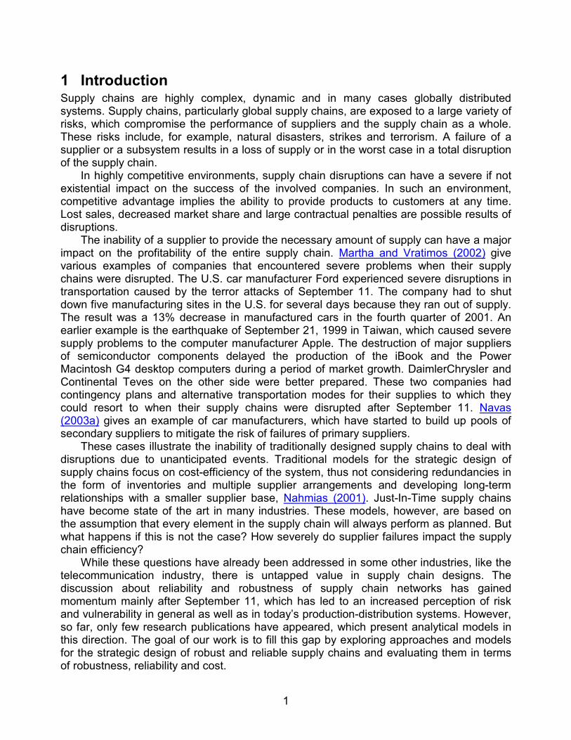
1 Introduction Supply chains are highly complex, dynamic and in many cases globally distributed systems. Supply chains, particularly global supply chains, are exposed to a large variety of risks, which compromise the performance of suppliers and the supply chain as a whole. These risks include, for example, natural disasters, strikes and terrorism. A failure of a supplier or a subsystem results in a loss of supply or in the worst case in a total disruption of the supply chain.

In highly competitive environments, supply chain disruptions can have a severe if not existential impact on the success of the involved companies. In such an environment, competitive advantage implies the ability to provide products to customers at any time. Lost sales, decreased market share and large contractual penalties are possible results of disruptions.

The inability of a supplier to provide the necessary amount of supply can have a major impact on the profitability of the entire supply chain. Martha and Vratimos (2002) give various examples of companies that encountered severe problems when their supply chains were disrupted. The U.S. car manufacturer Ford experienced severe disruptions in transportation caused by the terror attacks of September 11. The company had to shut down five manufacturing sites in the U.S. for several days because they ran out of supply. The result was a 13% decrease in manufactured cars in the fourth quarter of 2001. An earlier example is the earthquake of September 21, 1999 in Taiwan, which caused severe supply problems to the computer manufacturer Apple. The destruction of major suppliers of semiconductor components delayed the production of the iBook and the Power Macintosh G4 desktop computers during a period of market growth. DaimlerChrysler and Continental Teves on the other side were better prepared. These two companies had contingency plans and alternative transportation modes for their supplies to which they could resort to when their supply chains were disrupted after September 11. Navas (2003a) gives an example of car manufacturers, which have started to build up pools of secondary suppliers to mitigate the risk of failures of primary suppliers.

These cases illustrate the inability of traditionally designed supply chains to deal with disruptions due to unanticipated events. Traditional models for the strategic design of supply chains focus on cost-efficiency of the system, thus not considering redundancies in the form of inventories and multiple supplier arrangements and developing long-term relationships with a smaller supplier base, Nahmias (2001). Just-In-Time supply chains have become state of the art in many industries. These models, however, are based on the assumption that every element in the supply chain will always perform as planned. But what happens if this is not the case? How severely do supplier failures impact the supply chain efficiency?

While these questions have already been addressed in some other industries, like the telecommunication industry, there is untapped value in supply chain designs. The discussion about reliability and robustness of supply chain networks has gained momentum mainly after September 11, which has led to an increased perception of risk and vulnerability in general as well as in today’s production-distribution systems. However, so far, only few research publications have appeared, which present analytical models in this direction. The goal of our work is to fill this gap by exploring approaches and models for the strategic design of robust and reliable supply chains and evaluating them in terms of robustness, reliability and cost.

2

We focus on the design of inbound supply chains that incorporate reliability and

robustness. To the best of our knowledge, we are the first ones to give analytical models for the inbound supply chain design that embed cost, reliability and robustness. We introduce three new concepts:

supply chains with low probabilities of supplier failures, supply chains with emergency buffers and contingency supply, and supply chains with expected service level.

We explore the trade-offs among cost, reliability and robustness. In Section 2 we present the models for robust and reliable supply chains in detail. In

Section 3 we introduce a case study, we evaluate the proposed models, and we discuss the results of the different models. We conclude the introduction by explaining basic concepts and by giving a review of the related literature.

1.1 Concepts We define reliability as the probability that a system or a component performs its specified function as intended within a given time horizon and environment. A system consisting of different components can only perform as intended if every component fulfils its system-relevant functions. In other words, reliability refers to the probability of the absence of failures affecting the performance of the system over a given time interval and under given environmental conditions, Kuo and Zuo (2003), Andrews and Moss (2002).

In the context of supply chain management, supplier (component) and supply chain (system) reliability have to be distinguished. Supplier reliability refers to the probability that the supplier operates as planned during the planning horizon. In our work, we define failure as the inability of a supplier to ship any of the required amounts of material to its customers for a certain duration of time. Failures result from various reasons, such as strikes, destruction of production facilities (e.g. due to a fire), natural disasters, sabotage, terrorism or war.

The term supply chain reliability is used to express the probability of a supply chain to completely fulfill the demand of a final product without any loss of supply resulting from failures of suppliers. Thus, any supplier failure compromises supply chain reliability.

We assume that a supplier either delivers zero or the full amount of its designated supply. Partial failures of supplier nodes with a reduced output are not considered in this context, but they are part of future research. Let vr denote the reliability of a supplier v over the strategic supply chain planning horizon. The failure probability of supplier v is

vv rp −= 1 . Assuming independent supplier reliabilities, supply chain reliability R can be

calculated as the product of all individual supplier reliabilities in the supply chain:

∏=vvrR

suppliers all

. ( 1 )

Robustness on the other hand deals with the impact of failures on the performance of a system. The term robustness can be defined in many ways, depending on the specific context. For an overview of working definitions of robustness see for example the report by the Santa-Fe Institute (2001). We define robustness as the extent to which a system is able to perform its intended function relatively well in the presence of failures of components or subsystems. In the context of our work, we use robustness to describe how

3

much the output of a supply chain is affected by supplier failures. Output refers to the amount of products that are manufactured during the planning horizon. The failure of a supplier interrupts the downstream material flow originating from the failed node and leads to a reduction of the overall available supply for the production of the final product. Thus, robustness assesses the reduction of the output, whereas reliability can be used to quantify the likelihood of a reduction of any magnitude. Robustness of a supply chain cannot be as easily quantified as reliability. We capture two aspects of supply chain robustness that we also quantify. The first one being the number of supplier failures before a supply chain is completely disrupted. The second is the standard deviation of the output, which is a common measure for risk-induced variability of performance indicators. The standard deviation however is strongly influenced by reliability as well.

1.2 Literature Review Next we provide a review of how risk in general and the risk of supplier failures in particular have been discussed in the supply chain management literature. Supply chains face various sources of risk. Besides manufacturing processes and customer demand, Davis (1993) identifies the performance of suppliers as a major source of risk which influences the efficiency of a supply chain. Van der Vorst et al. (1998) name order forecast horizon, input data, administrative and decision processes as well as inherent uncertainties depending on the typology of the supply chain as major risk clusters. Van Landeghem and Vanmaele (2002) present a list of various sources of uncertainty that endanger the efficiency of global supply chains and indicate the most appropriate supply chain planning level to address them. Risks incurred due to demand variations and information distortion are classical issues in the supply chain management literature. The effect of demand volatility amplification along the supply chain due to information distortion is called the “bullwhip effect” and was first discovered by Forrester (1961). Based on Forrester’s findings, research on this effect has been elaborated by many other authors, see e.g. Lee, Padmanabhan and Whang (1997) for a recent reference.

In the supply chain management literature, risk has been addressed mainly on the tactical planning level focusing on uncertainty of demand or lead-times. Safety stocks are the means to reduce the effects of these types of uncertainties. For an overview of the vast literature on safety stock see for example the survey articles by Axsäter (1993), Federgruen (1993), Inderfurth (1994), van Houtum et al. (1996) or Diks et al. (1996).

In distribution systems, warehouses between manufacturers and retailers are used to buffer lead-time or demand uncertainties. Schwarz and Weng (2000) provide recent references on the risk pooling literature. A comprehensive review of earlier references on this subject can be found in Schwarz (1989).

Van Landeghem and Vanmaele (2002) introduce a robust planning approach to tactical supply chain planning under uncertainty. Monte Carlo simulation is used to characterize joint distributions of performance outcomes to allow for better decision-making, e.g. in terms of safety stock levels or for the identification of uncertain factors with large impacts on the supply chain performance.

Among the extensive literature on strategic supply chain design only few authors consider the design of supply chains under different aspects of uncertainty. For a literature review on strategic supply chain design, we refer to the survey articles of Vidal and Goetschalckx (1997) and Goetschalckx (2000). Literature on reliability or robustness of supply chain networks is even more scarse. Vidal and Goetschalckx (2000) present a survey of stochastic elements that have been included by various authors in models for

4

global supply chain design. Most of these analytical models address mainly financial risks, such as exchange rate fluctuations or uncertain market prices, see e.g. Hodder and Dincer (1986), Huchzermeier (1991) and Huchzermeier and Cohen (1996).

Vidal and Goetschalckx (2000) present an approach that includes supplier reliability as a design criterion. A constraint is formulated which guarantees that the probability of all suppliers of critical materials of being on time satisfies at least a given target probability at each plant in the network. This concept is formulated only for the case that all suppliers directly ship to the manufacturing plants.

Sheffi (2001) suggests dual supply arrangements in a strategic supply chain design. Except for a small illustrative example, no analytical formulations for a strategic supply chain model are provided. The author also opts for the installation of strategic emergency stock in the supply chain. Again, no analytical formulations for the integration of this concept into strategic design models are given.

Snyder and Daskin (2003) introduce a facility location model, which performs well under both normal operating conditions and when distribution centers in the network fail. Retail nodes in a distribution system are assigned to a hierarchy of distribution centers. If a distribution center on a higher level in this hierarchy fails, the retailer will then be served by the one on the next lower stage.

Though the literature on supply chain management lacks on the topic of network robustness and reliability, this has been discussed extensively in the literature on the design of survivable telecommunication networks. Survivable networks are defined as networks that are still functional after a failure of certain network components (see e.g. Soni and Pirkul (2000)). Network and cost structure of these networks, however, differs significantly from those of supply chain networks. The focus of survivable communication networks is to ensure the connectivity of the network in case of failures, which is clearly not an objective in supply chain problems.

2 Models for Robust and Reliable Supply Chains The goal of this work is to create a robust and reliable, yet economical, inbound supply chain for a manufacturer of a given final product. An integrated multi-echelon supply chain is considered, comprising of multiple production stages for the components of either the final product or other intermediary components. We focus on long-term contracting of supply arrangements for a strategic supply chain planning horizon.

Our models for the strategic design of robust and reliable supply chains build upon a base model, which is the traditional model for strategic supply chain design. The objective function of the base model is to minimize production and fixed costs subject to constraints for meeting the demand of the final product, flow balancing, and production capacity limitations. This model does not incorporate aspects of reliability or robustness.

A model for supply chains with increased reliability is obtained by adding a constraint to the base model, which specifies that the supply chain reliability (1) be larger than a given target reliability. Robustness of a supply chain can be improved by building redundancy into the system. A model with additional suppliers is obtained by adding constraints, called the supplier sourcing limits, to the base model that enforce bounds on the amount of supply a customer can source from a single supplier. In addition, we develop a contingency supply model. This model does not only reduce the risk of failing completely by having additional suppliers, but it also accounts for a partial compensation of the loss.

5

While the reliability model, according to our definition, focuses only on the occurrence of failures but does not consider the supply reduction, robustness, on the other hand, is primarily concerned with the amount of supply still available in the presence of failures, but it disregards the likelihood of such an event.

It is clearly desirable to combine both concepts into a joint reliability-robustness model for the design of supply chains, which are first, less likely to fail and second, still provide sufficient supply in the case of failures. We achieve this by a model that considers expected flows, subject to satisfying a given target service level. This model combines probabilistic aspect of reliability with the quantitative aspects of robustness.

Another formulation for integrating robustness and reliability is obtained by adding both supplier sourcing limit and target supply chain reliability constraints to the base model.

All supply chain networks resulting from the different models outlined above are evaluated with respect to a solution of the base model. To allow for a more descriptive evaluation of the performance of the various supply chains in terms of robustness, reliability, and cost as well as to illustrate their characteristics, a fictitious case study is introduced to which the different models are applied.

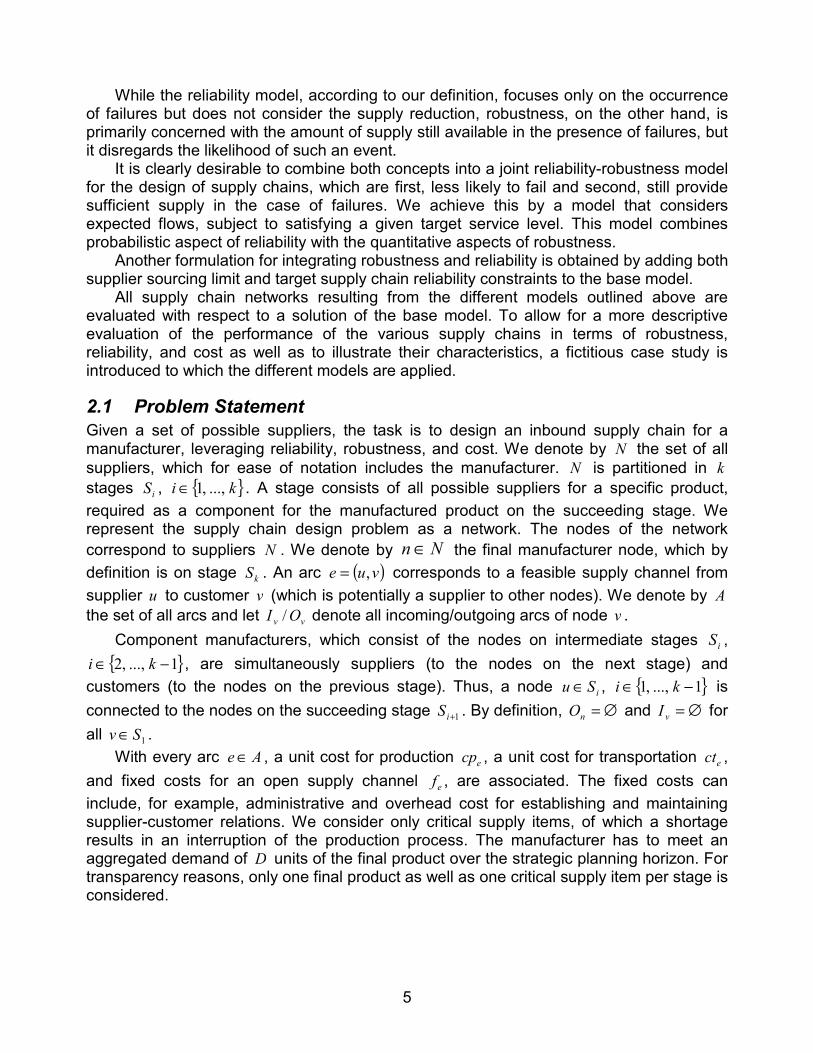
2.1 Problem Statement Given a set of possible suppliers, the task is to design an inbound supply chain for a manufacturer, leveraging reliability, robustness, and cost. We denote by N the set of all suppliers, which for ease of notation includes the manufacturer. N is partitioned in k stages iS , { }ki ...,,1∈ . A stage consists of all possible suppliers for a specific product, required as a component for the manufactured product on the succeeding stage. We represent the supply chain design problem as a network. The nodes of the network correspond to suppliers N . We denote by Nn∈ the final manufacturer node, which by definition is on stage kS . An arc ( )vue ,= corresponds to a feasible supply channel from supplier u to customer v (which is potentially a supplier to other nodes). We denote by A the set of all arcs and let vv OI / denote all incoming/outgoing arcs of node v .

Component manufacturers, which consist of the nodes on intermediate stages iS , { }1...,,2 −∈ ki , are simultaneously suppliers (to the nodes on the next stage) and

customers (to the nodes on the previous stage). Thus, a node iSu∈ , { }1...,,1 −∈ ki is connected to the nodes on the succeeding stage 1+iS . By definition, ∅=nO and ∅=vI for all 1Sv∈ .

With every arc Ae∈ , a unit cost for production ecp , a unit cost for transportation ect , and fixed costs for an open supply channel ef , are associated. The fixed costs can include, for example, administrative and overhead cost for establishing and maintaining supplier-customer relations. We consider only critical supply items, of which a shortage results in an interruption of the production process. The manufacturer has to meet an aggregated demand of D units of the final product over the strategic planning horizon. For transparency reasons, only one final product as well as one critical supply item per stage is considered.

6

2.2 Base Model The base model is a deterministic mixed integer programming model. It has two types of decision variables. For every arc Ae∈ , the binary variable eY is one, if this link is used in the supply chain and zero, if it is inactive. The continuous variable eX represents the amount of units flowing along arc e . A flow 0>eX can only be assigned to an arc if it is active, i.e. 1=eY .

The objective function of the base model is to minimize the total production, transportation and fixed costs, given by:

( )[ ]∑∈

⋅+⋅+Ae

eeeee YfXctcp . ( 2 )

For every Uk

iiSv

2=

∈ , let vα be the bill-of-materials parameter that expresses how many

input units are required for the production of one output unit. The sum of the incoming material flows to the final manufacturer node must equal the aggregated demand D , multiplied by the bill-of-materials parameter, which is expressed as

DX nen

⋅=∑∈

αIe

. ( 3 )

Nodes on intermediate stages iS , { }1,...,2 −∈ ki are technically transshipment nodes, for which the total flow into this node has to equal the total flow out. The supply inputs to these nodes are transformed into component flows to the next stage, considering the bill-of-materials relationship. The following flow balancing constraints

∑∑∈∈

⋅=vv

eve XXOeIe

α for all U1

2

−

=

∈k

iiSv ( 4 )

guarantee that there are no additional sources than those on the first stage and no additional sinks except the end manufacturer node. Each supplier v has a production capacity limit vm that must not be exceeded:

ve mv

≤∑∈Oe

X for all { }nNv /∈ . ( 5 )

With every arc e , a minimum flow eq is associated. This represents, for example, minimum order quantities demanded by the suppliers and prevents unreasonably low flows.

ee XYq ≤⋅ e for all Ae ∈ ( 6 )

The following constraints guarantee that flows can only be assigned to active arcs:

ee YMX ⋅≤ for all Ae ∈ ( 7 )

In these inequalities, M is an auxiliary parameter representing a large enough number. For the uncapacitated case, i.e. ∞=vm for all Nv∈ , it can be shown that the supply

chain resulting from the base model is always a serial supply chain. This type of a supply chain has only one supplier per stage and the critical supply items flow along a single path from the supplier on the first stage to the end manufacturer. This makes the supply chain

7

extremely vulnerable to failures of suppliers. The overall performance critically depends on the performance of each and every supplier in the network. The image that a chain can only be as strong as its weakest link applies here: the entire chain can only perform well if each and every supplier performs well. A failure of a single supplier disrupts the entire supply chain. Therefore a serial supply chain is not robust at all.

As the presented network design model is based only on lowest possible cost, typically the supply chain reliability is relatively low, too, because the cheapest suppliers are in all likelihood not the most reliable ones. In most cases a negative relationship between reliability and cost is a realistic assumption.

In a first step towards less risk of severe disruptions, the supply chain can be improved by choosing a more reliable supplier on each stage. As these tend not to be the cheapest suppliers, higher costs are incurred which leads to the problem of leveraging reliability and profitability of the chain.

2.3 Reliability Model We extend the approach of Vidal and Goetschalckx (2000) to multi-stage supply chains by adding a new constraint to the base model, which enforces the supply chain reliability to be greater or equal than the desired target supply chain reliability R . For every { }nNv /∈ , let vZ be a binary variable indicating if a supplier is used or not. Then based on (1) the

reliability of the supply chain is

{ }

RrnNv

Zv

v ≥∏∈ /

. ( 8 )

This nonlinear expression is linearized by applying the logarithm on both sides. This yields the inequality

( ) ( )RZrnNv

vv loglog}/{

≥⋅∑∈

, ( 9 )

which is linear. We link vZ and eX by ),( uvv XZM ≥⋅ for all Avu ∈),( ( 10 ) ),( uvv YZ ≤ for all ( ) Auv ∈, . ( 11 )

From the computational point of view, it suffices to include only a single family of constraints. However, we list both to adhere with the definition of Z . The reliability model consists of the objective function (2), constraints (3)-(7) and (9)-(11).

In the uncapacitated case, it is shown in Bundschuh (2003) that this model yields a serial supply chain. The obtained supply chain now has a lower risk of failing, but the effect of a supplier failure remains the same. If a single element in the serial chain fails, it disrupts the entire chain. To further improve the performance of the supply chain, fail-safe features have to be included.

2.4 Robustness Models Reducing the impact of failures on the output of the supply chain and thus making it more robust can be achieved by building redundancy into the network, i.e. increasing the number of suppliers on each stage. In case of a failure the remaining unaffected suppliers still provide their share of the total demand of critical supply. The supply chain is now much

8

less likely to be completely disrupted, since for a complete disruption all suppliers on the same stage have to fail simultaneously. On the other hand, using more suppliers increases the fixed costs. In addition to using only the cheapest suppliers we have to opt for more expensive ones.

2.4.1 Supplier Sourcing Limit Model One way of creating a supply chain with redundant suppliers is to add sourcing limit constraints to the base model. The sourcing limits impose an upper bound on the amount of critical supply a node can source from a single supplier. The upper bound is expressed in terms of a given percentage ω of the total demand of the node. The supplier sourcing limit constraints

∑∈

⋅≤vIe

ee XX ω for all Uk

iiSv

2=

∈ , for all vIe∈ ( 12 )

are added to the model. The supplier sourcing limit model consists of the objective function (2), constraints (3)-(7) and (12).

The sourcing limit formulation however does not consider supplier reliabilities. It is solely concerned with minimizing the magnitude of a supply loss in case of a failure but not the probability of its occurrence. On the contrary, using now more suppliers than in a serial supply chain, reliability is drastically reduced, because every additional supplier increases the risk of a failure. Compared to the reliability model, the supply chain network designed with the sourcing limit constraints has a much higher probability of the occurrence of a failure, but less severe effects in the actual case of a failure, because the redundant suppliers leverage the loss.

The core idea of redundancy is to reduce risk by distributing it. Unless all suppliers on a stage fail simultaneously, the loss due to a failure of one or more suppliers no longer leads to a complete shortage of critical supply, but still to a reduction of the total available supply in the supply chain. This shortcoming of the supplier sourcing limit approach can be eliminated by expanding it with features for a partial compensation of the loss, which further improve the mean output and the standard deviation of the output, and increase the degree of robustness of the supply chain.

2.4.2 Contingency supply model Compensation for a loss of supply is achieved by having contingency supply at hand in case of a failure. There are two possible ways of implementing contingency supply in a supply chain. The first possibility is to install strategic emergency buffers (SEBs), as proposed by Sheffi (2001), which are used only in case of a supply disruption. These buffers contain critical supply items needed for the production of additional components to compensate for a loss of supply. Unlike conventional safety stock, the SEBs are not used to hedge against stochastic demand. Using solely SEBs is very expensive, because the SEB inventory levels would be significant if sufficient loss compensation is to be guaranteed.

A second possibility that prevents a large accumulation of emergency inventory is the purchase of options on additional supply in case of a loss. In case of a failure, the remaining suppliers provide extra supply in addition to their regular contractual supply to make up for at least a given percentage of the loss. As opposed to the SEBs, this form of contingency supply is physically not existent in the supply chain. It is only made available if a shortage occurs. This poses the problem of the lead-time of the contingency supply.

9

Every node has a certain production and transportation lead-time until the contingency supply is made available to its customers. After this time, the customers, which themselves are suppliers of contingency supply to their customers on the next stage, can begin the production of the additional units and even more time elapses until the contingency supply reaches the next stage, and so forth. The total lead-time until the first contingency supply items reach the end manufacturer can be considerable and this may or may not be acceptable, depending if the excess demand of the final product in case of a supply shortage can be back-ordered or is lost. A reasonable strategy is to combine SEB with options on contingency supply. In this strategy the SEB at a supplier node is used to bridge the lead-time until the suppliers of this node are able to provide additional contingency units. With this combination strategy we are able to compensate for the loss of supply due to supplier failures at any time in an economical way. However, the cost structure of this type of problem is more complicated, because the cost of an option and the costs for purchasing and holding the buffers have to be included.

In this model we need two new decision variables vU and eS . For every Uk

iiSv

2=

∈ , vU

is the decision variable for the size of the SEB kept at node v and for every Ae∈ , eS denotes the amount of contingency supply units for the option between the nodes connected by arc e .

For setting up a supply chain with contingency supply, additional costs are incurred by the SEBs and the options on contingency supply. Additional critical supply must be purchased for the storage in the SEBs. Except for these initial set-up costs, the SEBs also incur ongoing holding costs. The parameter vh expresses the per unit holding cost at node v . Purchasing options on contingency can be viewed as buying insurance for a loss of supply. The supplier as insurance provider has to either keep free production capacity in case the contingency supply is needed or to be able to free capacity within a certain time. The price for this service, the risk prime, is expressed as an extra charge on the production cost of the regular units, depending on the amount of contingency supply. If the option on contingency supply has to be realized, the production cost of these additional supply items is assumed to be higher than those of the regular units. Since we are dealing with the strategic design of a supply chain, these additional production costs are not captured in the model, because they are only incurred in case of a failure. However, the failure costs are considered implicitly in an extension of this model to a combined reliability-robustness model, described in Section 2.5.2.

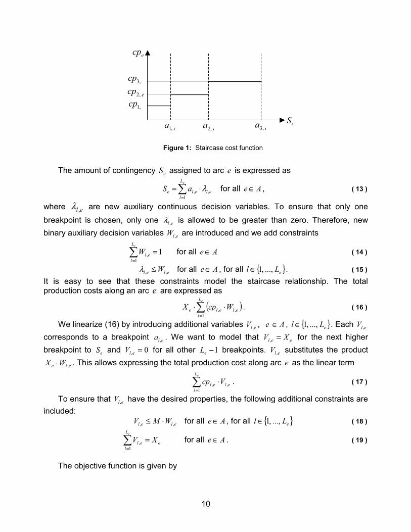
The unit production cost of regular supply is described as a function of the amount of contingency supply eS (staircase cost). At given breakpoint quantities of eS , the per unit cost increases to a higher value and is constant over the interval until the next breakpoint is reached. The breakpoints of arc e are denoted by ela , , { }eLl ...,,1∈ , where eL is the number of breakpoints. The piecewise constant production costs associated with each one of these breakpoints are denoted as elcp , , { }eLl ...,,1∈ . Figure 1 depicts the notation for

eL = 3. For example, if on arc e we contract eS , eee aSa ,3,2 ≤≤ units of contingency supply, then the per unit cost of the regularly contracted units eX is ecp ,3 .

10

Figure 1: Staircase cost function

The amount of contingency eS assigned to arc e is expressed as

∑=

⋅=eL

lelele aS

1,, λ for all Ae∈ , ( 13 )

where el ,λ are new auxiliary continuous decision variables. To ensure that only one breakpoint is chosen, only one el ,λ is allowed to be greater than zero. Therefore, new binary auxiliary decision variables elW , are introduced and we add constraints

∑=

=eL

lelW

1, 1 for all Ae∈ ( 14 )

elel W ,, ≤λ for all Ae∈ , for all { }eLl ...,,1∈ . ( 15 ) It is easy to see that these constraints model the staircase relationship. The total production costs along an arc e are expressed as

( )∑=

⋅⋅eL

lelele WcpX

1,, . ( 16 )

We linearize (16) by introducing additional variables elV , , Ae ∈ , { }eLl ...,,1∈ . Each elV , corresponds to a breakpoint ela , . We want to model that eel XV =, for the next higher breakpoint to eS and 0, =elV for all other 1−eL breakpoints. elV , substitutes the product

ele WX ,⋅ . This allows expressing the total production cost along arc e as the linear term

∑=

⋅eL

lelel Vcp

1,, . ( 17 )

To ensure that elV , have the desired properties, the following additional constraints are included:

elel WMV ,, ⋅≤ for all Ae∈ , for all { }eLl ...,,1∈ ( 18 )

e

L

lel XV

e

=∑=1

, for all Ae∈ . ( 19 )

The objective function is given by

eSea ,1 ea ,2 ea ,3

ecp

ecp ,2

ecp ,3

ecp ,1

11

∑∑ ∑=

∈∈ =

⋅+

⋅+⋅+⋅

Uk

i

e

vvAe

eeee

L

lelel UhYfXctVcp

2iS v

1,, . ( 20 )

The first term captures the cost for production, transportation as well as for the options on contingency supply, and the second term expresses the holding cost for the inventoried critical supply in the SEBs.

By using a contingency supply arrangement we can model a maximum tolerable loss. Because of the relatively low probability of two or more suppliers or an entire region failing, it is reasonable to set a maximum tolerable loss only for the case of a single supplier failure. Assuming a single supplier failure, we would like the loss not to exceed D⋅µ , where µ is the maximum tolerable loss percentage in terms of the demand of the final product. This means that for a failure of supplier w on stage iS , the regular flows eX and the emergency flows eS of the remaining suppliers on the same stage iS , in addition to the sum of the SEBs kept at nodes on the succeeding stage 1+iS , must be at least µ−1 percent of the total regular output of stage iS . Formally this is expressed as

( ) ( ) ( ) ∑ ∑∑∑∑ ∑∈ ∈∈∈∈ ∈

⋅−≥++−++ i viwi v Sv OeSu

uOeSv Oe

U eeeee X1XSXS1

µ ( 21 )

for all iSw∈ , for all { }1...,,1 −∈ ki . An option of contingency supply can only be purchased in addition to regular supply,

which is captured by ee YMS ⋅≤ for all Ae∈ . ( 22 ) The contingency output of a node on an intermediary stage has to be covered by its

SEB and additional contingency options from its suppliers. A node only needs to purchase enough options on contingency supply from its suppliers to cover that part of its contingency output that is not already stored in the SEB. Thus, the contingency supply output of an intermediate node v must equal the contingency flows into this node in addition to its SEB, considering the bill-of-materials parameter vα :

+⋅= ∑∑

∈∈v

IevOeU

vv

ee S1Sα

for all U1

2

−

=

∈k

iiSv . ( 23 )

Outgoing contingency and regular flows out of a node cannot exceed the production capacity. Therefore, the supplier capacity limit (5) from the base model has to be modified to account for the contingency flows as well. The new constraints read

( ) vee mv

≤+∑∈ Oe

SX for all U1

1

−

=

∈k

iiSv . ( 24 )

The installation of the SEB requires modifications of (3) and (4). For the final manufacturer node the total inflow of regular supply has to equal the final demand plus the size nU of the SEB at this node considering the bill-of-materials relationship.

nne UDXn

+⋅=∑∈

αIe

( 25 )

Similarly, the input of regular supply to node v on an intermediate stage must be equal to its output of regular supply, with respect to the bill-of-materials relationship, plus the amount vU , needed for the installation of the SEB at this node.

12

∑∑∈∈

⋅+=vv

evvIe

e UXOe

Xα for all U1

2

−

=

∈k

iiSv ( 26 )

The SEB at a node v on an intermediate stage is used to cover the supply, which is needed for the production of contingency components during the lead-time until the suppliers of this node are able to provide the necessary contingency supply. If vτ denotes the maximum lead time until the suppliers on the preceding stage provide the contingency supply to node v , then the requirement for the minimum buffer size of the SEB is expressed as

∑∈

⋅⋅≥vOe

vvvU eSατ for all U1

2

−

=

∈k

iiSv . ( 27 )

The minimum buffer size of the final manufacturer node has to cover the supply for the production of at least µ−1 percent of the demand of final product during the maximum lead-time of its suppliers on stage 1−kS and therefore we need

DU nnn ⋅⋅⋅≥ µτα . ( 28 )

Typically, the physical storage of a SEB is upper bounded. If vU denotes the maximum size of the SEB at node v , we add

vv UU ˆ≤ for all Uk

iiSv

2=

∈ . ( 29 )

In order to reduce the amount of contingency supply, and thus the cost, this model tends to use a larger number of suppliers per stage. To prevent this, an upper limit on the number of suppliers iN on stage iS is imposed by adding

iSv

v NZi

≤∑∈

for all { }1...,,1 −∈ ki , ( 30 )

where the binary variables vZ indicate if a supplier is used or not. To link vZ to the rest of the model, constraints (10) and (11) are needed. Finally, as this model is an extension of the supplier sourcing limit model the supplier sourcing limit constraints (12) have to be included. The contingency supply model has the objective function (20), constraints (6)-(7), (10)-(15), (18)-(19) and (21)-(30).

Like the sourcing limit model, the contingency supply model does not take the supplier reliabilities into account. Choosing cheap but unreliable suppliers leads to a higher expected failure cost, since it is much more likely that the options on contingency supply have to be used and the increased production cost for the additional units have to be paid.

2.5 Combined Reliability - Robustness Models It is desirable to have a robust and reliable supply chain for the critical supply items. The likelihood of supplier failures should be sufficiently small as well as the loss of supply. We introduce two formulations for combined reliability-robustness models.

2.5.1 Expected Service Level Model A model which considers the expected values of the material flows subject to meeting a given target service level is a possible way of combining robustness and reliability. The expected value of a material flow reflects both quantitative and probabilistic aspects. The expected service level methodology consists of two phases and considers the regular

13

flows eX and their expected values eE . We proceed as follows. In the first phase we obtain from a model the expected flow values such that the expected costs are minimized. The regular flows are assigned preliminarily for the calculation of the expected flows and that the demand is met as well as that the supplier capacity constraints are not violated. The preliminary regular flows are denoted by eX . In the second phase, the regular flows are reassigned based on the as-ordered rationing. By as-ordered rationing we mean that the total expected output of a supplier node is distributed among the customer nodes according to their ordered shares of the regular output.

In the first phase, the deterministic objective function (2) of the base model is changed to

( )[ ]∑∈

⋅+⋅+Ae

eeeee YfEctcp . ( 31 )

The expected service level is the sum of the incoming expected flows into the manufacturer divided by the demand and the bill-of-materials parameter. The constraint

DSLE nen

⋅⋅≥∑∈

αIe

( 32 )

expresses that the expected service level has to be greater or equal than a given target service level SL . At the first stage, basic probability shows that

),(),(ˆ

vuuvu XrE ⋅= for all ),( vu . ( 33 ) Similarly, for any node v on intermediate stages, the expected value of the output

equals the expected flow into this node multiplied by its reliability vr and divided by the bill-of-materials parameter vα . This yields

∑∑∈∈

⋅=vv

ev

ve E

rE

IeOe α for all U

1

2

−

=

∈k

iiSv . ( 34 )

Clearly, the expected flows can be positive only on open supply channels, ee YME ⋅≤ for all Ae∈ . ( 35 ) To improve robustness of supply chains designed with the expected service level

model supplier sourcing limit constraints are included. These constraints are very similar to (12), except that now only a given percentage of the expected value of the input flows to a node can be provided by a single supplier.

∑∈

⋅≤vIe

ee EE ω for all Uk

iiSv

2=

∈ ( 36 )

Supplier capacity constraints, flow balancing constraints for regular flows and the constraint for meeting the demand of the final product are identical to the corresponding base model constraints (3)-(5) (except that eX are replaced by eX

().

The following two families of constraints guarantee that regular flows can only be assigned to arcs with positive expected values of flows and that the expected value of flow is less or equal to the regular flow.

ee EMX ⋅≤ˆ for all Ae∈ ( 37 )

ee XE ˆ≤ for all Ae∈ ( 38 ) The minimum order quantities are expressed as

14

ee EYq ≤⋅ e for all Ae∈ . ( 39 ) Note that since ee EX ≥ˆ , the minimum order quantity constraint cannot be violated by the regular flow. The expected service level model consists of the objective function (31) and has constraints (3)-(5), (32)-(36) and (37)-(39).

After solving this model in the first phase, we next reassign the regular flow by using the expected flow. We proceed from the first stage up to the last one. The regular flow between the first and the second stage is calculated by

u

vuvu r

EX ),(

),( = for all ),( vu , with 1Su∈ . ( 40 )

On every other stage the regular flow is computed using

∑∑ ∈∈

⋅=v

v

Iee

Oee

ee X

EEX for all vOe∈ , for all U

1

2

−

=

∈n

iiSv . ( 41 )

Note that the incoming flows are determined by the preceding stage. It is easy to see that the computed eX satisfy constraints (3)-(5).

Further inclusion of a contingency-supply formulation into the expected service level model would lead to a very large and complex model which would be hardly tractable even for medium sized networks.

2.5.2 Reliability-Contingency Supply Model Another option of formulating a model for robust and reliable supply chains is to merge the reliability and contingency supply models. In this model the contingency supply model is augmented by the supply chain reliability constraint (9). With the resulting model the best results in terms of reliability and robustness should be produced, because the flows are not only distributed and backed-up with contingency supply but in addition more reliable suppliers are chosen to guarantee a given target supply chain reliability. However, higher costs are expected for this solution. The reliability-contingency supply model consists of objective function (20), constraints (6)-(7), (9)-(15), (18)-(19), and (21)-(30).

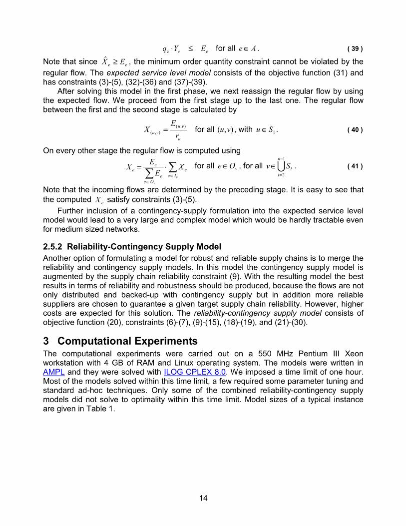
3 Computational Experiments The computational experiments were carried out on a 550 MHz Pentium III Xeon workstation with 4 GB of RAM and Linux operating system. The models were written in AMPL and they were solved with ILOG CPLEX 8.0. We imposed a time limit of one hour. Most of the models solved within this time limit, a few required some parameter tuning and standard ad-hoc techniques. Only some of the combined reliability-contingency supply models did not solve to optimality within this time limit. Model sizes of a typical instance are given in Table 1.

15

Model Total number of decision variables

Number of binary

variables Number of constraints Density

Base model 528 264 561 0.0051

Reliability model 568 304 898 0.0052

Supplier sourcing limit model 561 264 858 0.0049

Contingency supply model 3402 1096 4079 0.0008

Expected service level model (first step) 825 264 1515 0.0034

Reliability-contingency supply model 3402 1096 4080 0.0009

Table 1: Model sizes

Given a supply chain, its performance is analyzed by a simulation written in MATLAB.

In every scenario, we simulate failures of suppliers and determine the output of the supply chain from the “surviving” suppliers. Every reported result is based on a generation of 100,000 scenarios. The different models are compared and evaluated based on the

deterministic cost (given by the optimal value of the underlying model) for setting-up the supply chain network and contracting the flows, mean output, standard deviation of the output, number of supplier failures (how often the output of the supply chain is reduced due

to a failure of one or more suppliers), number of total disruptions (how often the output equals zero, because the failures

of suppliers destroy the material flows). The last four performance indicators are drawn from the simulation.

We have generated two instances. In the first instance, the manufacturer is located in North-America. The suppliers form 6 stages ( =k 6) and 4 geographical regions, which are North-America, Europe, South-America and South-East-Asia. Stages one through five consist of eight suppliers each and the last stage contains only the manufacturer node. Overall there are 41 nodes and 264 arcs. In figures that follow, the dots represent the supplier nodes and the triangle the final manufacturer. The aggregated demand of the final product over the strategic planning horizon of 5 years is assumed to be =D 1,000,000 units. We assume suppliers in North-America and Europe are more reliable, but also more expensive than those in the remaining two regions. The average supplier reliability in North-America and Europe is =avgr 0.98, the average production costs are =avgcp $41.8, as compared to =avgr 0.96 and =avgcp $25.6 in South-America and South-East-Asia. Fixed costs are assumed to be the same for all arcs == ff e $150,000. The minimum sourcing limits per arc of == qqe 70,000 units are imposed. Furthermore, every supplier is assumed to have sufficient production capacity so that production capacity limitations do not apply (i.e. ∞=vm for every v ). For simplicity, we assume all bill-of-materials parameters to be one, i.e. 1=vα for all nodes v .

16

For the contingency supply model we assume a staircase cost function with the same three breakpoints for every arc e : ea ,1 = 5,000 units, ea ,2 = 100,000 units, and ea ,2 = 250,000 units. The corresponding cost parameters are expressed relative to the production cost

ecp along the specific arc: ee cpcp =,1 , ecp ,2 = 1.05 ecp⋅ and ecp ,3 = 1.15 ecp⋅ . The upper bound on the number of suppliers per stage is 3 ( iN = 3 for i = 1, …, 5).

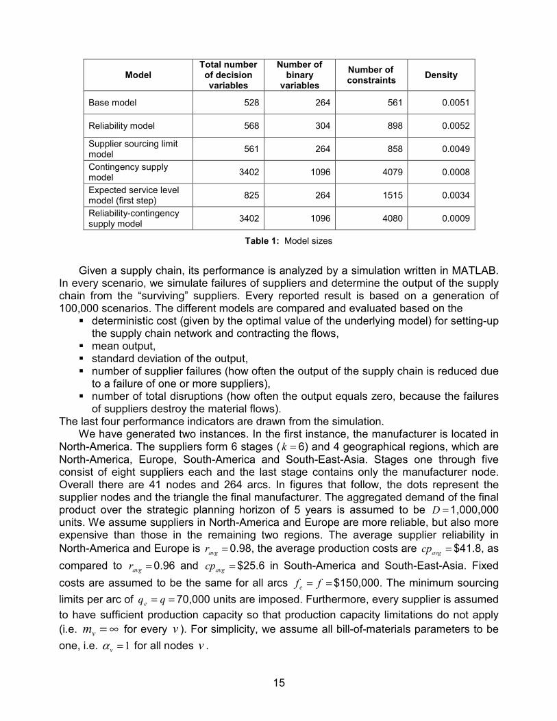
Applying the base model to this supply chain example, we obtain a supply chain with the cheapest, but unreliable suppliers, all of which are located either in South-America or South-East-Asia. This chain is shown in Figure 2.

Figure 2: Base model supply chain

The low reliabilities of the suppliers compromise the supply chain stability greatly and

expose it to a significant risk of disruption. Table 2 shows the results of this solution based on the simulation. In what follows, these values are set to 100% and the other models are evaluated with respect to these base model results.

Cost $ 146750000 Number of total failures 18386 Number of supplier failures 18386 Mean output 816140 Standard deviation of output 387372 Supply chain reliability (analytical) 0.8158

Table 2: Base model results

Though most cost-efficient, the base model supply chain exhibits a high probability of

approximately 18.4% of a complete disruption. In every serial supply chain the number of supplier failures equals the number of total supply chain disruptions, because the failure of any single supplier disrupts the only path to the manufacturer. The low mean output of 816,140 units and the high standard deviation of 387,372 units also reflect the questionable performance of the traditionally designed supply chains under the risk of supplier failures. The empirical reliability of 0.8161 obtained from the simulation is very close to the analytically calculated value of 0.8151, implying the correctness of the simulation based results.

Stage 1 Stage 2 Stage 3 Stage 4 Stage 5 Stage 6

Europe

South-America

North America

South-East-Asia

17

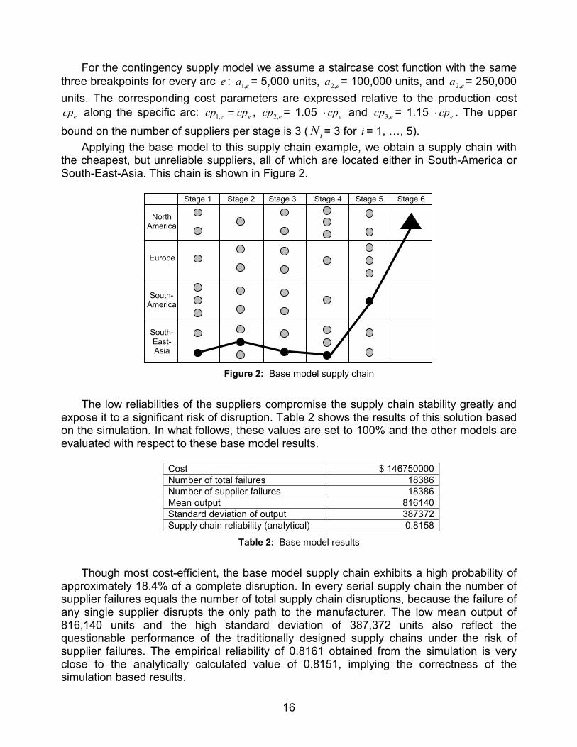
Using the reliability model, the high rate of total disruptions and thus the mean output and the standard deviation of the output can be improved drastically. Figure 3 shows the supply chains for a target supply chain reliability of =R 0.88 and for the maximum possible target supply chain reliability of =R 0.92.

Figure 3: Reliability model supply chain

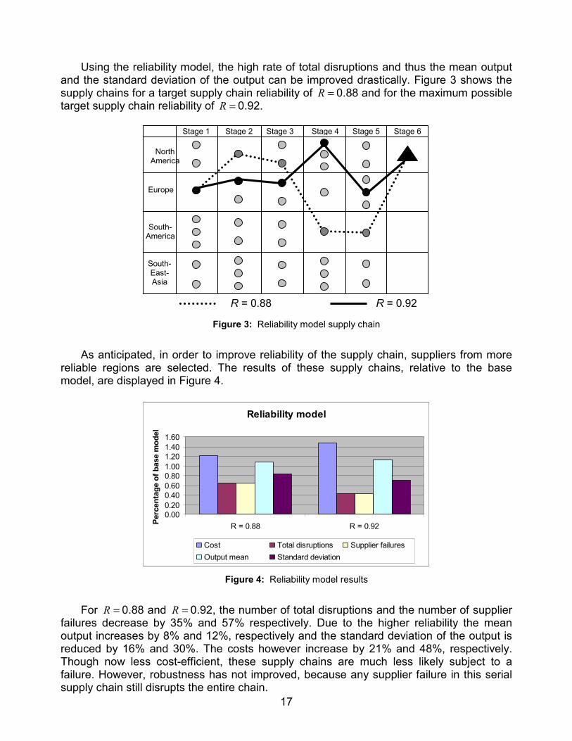
As anticipated, in order to improve reliability of the supply chain, suppliers from more

reliable regions are selected. The results of these supply chains, relative to the base model, are displayed in Figure 4.

Reliability model

0.000.200.400.600.801.001.201.401.60

R = 0.88 R = 0.92Perc

enta

ge o

f bas

e m

odel

Cost Total disruptions Supplier failuresOutput mean Standard deviation

Figure 4: Reliability model results

For =R 0.88 and =R 0.92, the number of total disruptions and the number of supplier

failures decrease by 35% and 57% respectively. Due to the higher reliability the mean output increases by 8% and 12%, respectively and the standard deviation of the output is reduced by 16% and 30%. The costs however increase by 21% and 48%, respectively. Though now less cost-efficient, these supply chains are much less likely subject to a failure. However, robustness has not improved, because any supplier failure in this serial supply chain still disrupts the entire chain.

R = 0.88 R = 0.92

Stage 1 Stage 2 Stage 3 Stage 4 Stage 5 Stage 6

Europe

South-America

South-East-Asia

North America

18

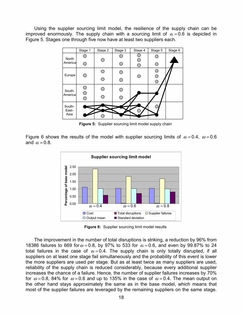
Using the supplier sourcing limit model, the resilience of the supply chain can be improved enormously. The supply chain with a sourcing limit of =ω 0.6 is depicted in Figure 5. Stages one through five now have at least two suppliers each.

Figure 5: Supplier sourcing limit model supply chain

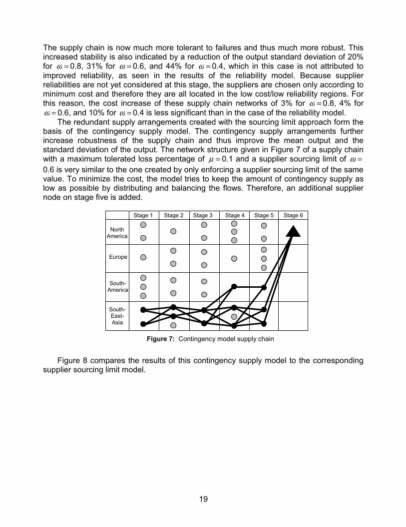
Figure 6 shows the results of the model with supplier sourcing limits of =ω 0.4, =ω 0.6 and =ω 0.8.

Supplier sourcing limit model

0.00

0.50

1.00

1.50

2.00

2.50

Perc

enta

ge o

f bas

e m

odel

Cost Total disruptions Supplier failuresOutput mean Standard deviation

Figure 6: Supplier sourcing limit model results

The improvement in the number of total disruptions is striking, a reduction by 96% from

18386 failures to 669 for =ω 0.8, by 97% to 533 for =ω 0.6, and even by 99.87% to 24 total failures in the case of =ω 0.4. The supply chain is only totally disrupted, if all suppliers on at least one stage fail simultaneously and the probability of this event is lower the more suppliers are used per stage. But as at least twice as many suppliers are used, reliability of the supply chain is reduced considerably, because every additional supplier increases the chance of a failure. Hence, the number of supplier failures increases by 70% for =ω 0.8, 84% for =ω 0.6 and up to 135% in the case of =ω 0.4. The mean output on the other hand stays approximately the same as in the base model, which means that most of the supplier failures are leveraged by the remaining suppliers on the same stage.

Stage 1 Stage 2 Stage 3 Stage 4 Stage 5 Stage 6

Europe

South-America

South-East-Asia

North America

=ω 0.4 =ω 0.6 =ω 0.8

19

The supply chain is now much more tolerant to failures and thus much more robust. This increased stability is also indicated by a reduction of the output standard deviation of 20% for =ω 0.8, 31% for =ω 0.6, and 44% for =ω 0.4, which in this case is not attributed to improved reliability, as seen in the results of the reliability model. Because supplier reliabilities are not yet considered at this stage, the suppliers are chosen only according to minimum cost and therefore they are all located in the low cost/low reliability regions. For this reason, the cost increase of these supply chain networks of 3% for =ω 0.8, 4% for

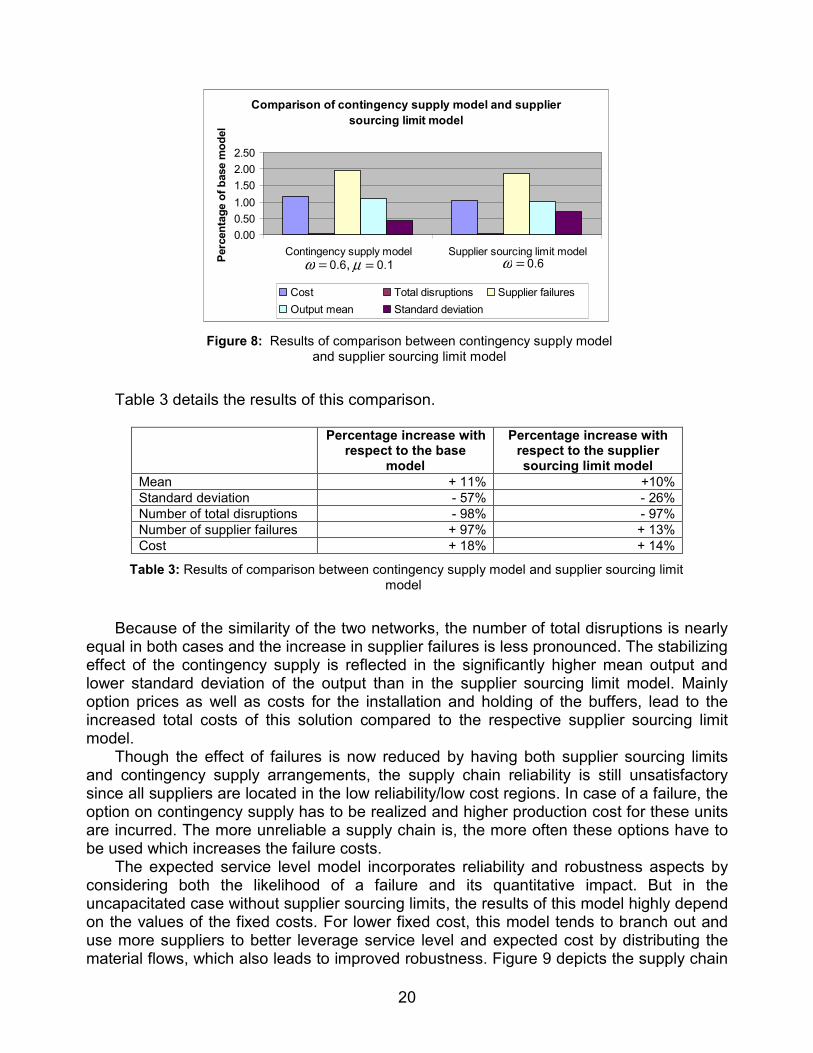
=ω 0.6, and 10% for =ω 0.4 is less significant than in the case of the reliability model. The redundant supply arrangements created with the sourcing limit approach form the

basis of the contingency supply model. The contingency supply arrangements further increase robustness of the supply chain and thus improve the mean output and the standard deviation of the output. The network structure given in Figure 7 of a supply chain with a maximum tolerated loss percentage of =µ 0.1 and a supplier sourcing limit of =ω 0.6 is very similar to the one created by only enforcing a supplier sourcing limit of the same value. To minimize the cost, the model tries to keep the amount of contingency supply as low as possible by distributing and balancing the flows. Therefore, an additional supplier node on stage five is added.

Figure 7: Contingency model supply chain

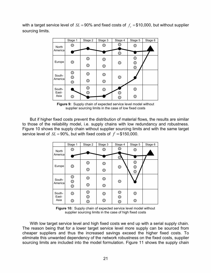
Figure 8 compares the results of this contingency supply model to the corresponding

supplier sourcing limit model.

Stage 1 Stage 2 Stage 3 Stage 4 Stage 5 Stage 6

Europe

South-America

South-East-Asia

North America

20

Comparison of contingency supply model and supplier sourcing limit model

0.000.501.001.502.002.50

Contingency supply model Supplier sourcing limit modelPerc

enta

ge o

f bas

e m

odel

Cost Total disruptions Supplier failuresOutput mean Standard deviation

Figure 8: Results of comparison between contingency supply model

and supplier sourcing limit model

Table 3 details the results of this comparison.

Percentage increase with

respect to the base model

Percentage increase with respect to the supplier sourcing limit model

Mean + 11% +10%Standard deviation - 57% - 26%Number of total disruptions - 98% - 97%Number of supplier failures + 97% + 13%Cost + 18% + 14%

Table 3: Results of comparison between contingency supply model and supplier sourcing limit model

Because of the similarity of the two networks, the number of total disruptions is nearly

equal in both cases and the increase in supplier failures is less pronounced. The stabilizing effect of the contingency supply is reflected in the significantly higher mean output and lower standard deviation of the output than in the supplier sourcing limit model. Mainly option prices as well as costs for the installation and holding of the buffers, lead to the increased total costs of this solution compared to the respective supplier sourcing limit model.

Though the effect of failures is now reduced by having both supplier sourcing limits and contingency supply arrangements, the supply chain reliability is still unsatisfactory since all suppliers are located in the low reliability/low cost regions. In case of a failure, the option on contingency supply has to be realized and higher production cost for these units are incurred. The more unreliable a supply chain is, the more often these options have to be used which increases the failure costs.

The expected service level model incorporates reliability and robustness aspects by considering both the likelihood of a failure and its quantitative impact. But in the uncapacitated case without supplier sourcing limits, the results of this model highly depend on the values of the fixed costs. For lower fixed cost, this model tends to branch out and use more suppliers to better leverage service level and expected cost by distributing the material flows, which also leads to improved robustness. Figure 9 depicts the supply chain

=ω 0.6, =µ 0.1 =ω 0.6

21

with a target service level of =SL 90% and fixed costs of =ef $10,000, but without supplier sourcing limits.

Figure 9: Supply chain of expected service level model without

supplier sourcing limits in the case of low fixed costs

But if higher fixed costs prevent the distribution of material flows, the results are similar

to those of the reliability model, i.e. supply chains with low redundancy and robustness. Figure 10 shows the supply chain without supplier sourcing limits and with the same target service level of =SL 90%, but with fixed costs of =f $150,000.

Figure 10: Supply chain of expected service level model without

supplier sourcing limits in the case of high fixed costs

With low target service level and high fixed costs we end up with a serial supply chain.

The reason being that for a lower target service level more supply can be sourced from cheaper suppliers and thus the increased savings exceed the higher fixed costs. To eliminate this unwanted dependency of the network robustness on the fixed costs, supplier sourcing limits are included into the model formulation. Figure 11 shows the supply chain

Stage 1 Stage 2 Stage 3 Stage 4 Stage 5

Europe

South-America

Stage 6

South-East-Asia

North America

Stage 1 Stage 2 Stage 3 Stage 4 Stage 5

Europe

South-America

Stage 6

South-East-Asia

North America

22

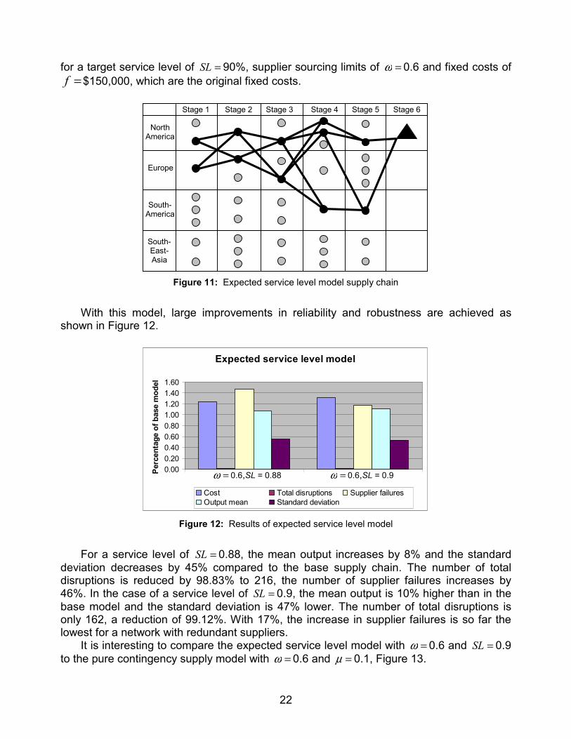
for a target service level of =SL 90%, supplier sourcing limits of =ω 0.6 and fixed costs of =f $150,000, which are the original fixed costs.

Figure 11: Expected service level model supply chain

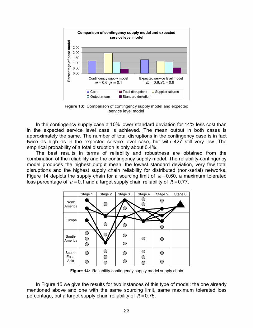
With this model, large improvements in reliability and robustness are achieved as

shown in Figure 12.

Expected service level model

0.000.200.400.600.801.001.201.401.60

Perc

enta

ge o

f bas

e m

odel

Cost Total disruptions Supplier failuresOutput mean Standard deviation

Figure 12: Results of expected service level model

For a service level of =SL 0.88, the mean output increases by 8% and the standard

deviation decreases by 45% compared to the base supply chain. The number of total disruptions is reduced by 98.83% to 216, the number of supplier failures increases by 46%. In the case of a service level of =SL 0.9, the mean output is 10% higher than in the base model and the standard deviation is 47% lower. The number of total disruptions is only 162, a reduction of 99.12%. With 17%, the increase in supplier failures is so far the lowest for a network with redundant suppliers.

It is interesting to compare the expected service level model with =ω 0.6 and =SL 0.9 to the pure contingency supply model with =ω 0.6 and =µ 0.1, Figure 13.

Stage 1 Stage 2 Stage 3 Stage 4 Stage 5

Europe

South-America

Stage 6

South-East-Asia

North America

=ω 0.6,SL = 0.88 =ω 0.6,SL = 0.9

23

Comparison of contingency supply model and expected service level model

0.000.501.001.502.002.50

Contingency supply model Expected service level modelPerc

enta

ge o

f bas

e m

odel

Cost Total disruptions Supplier failuresOutput mean Standard deviation

Figure 13: Comparison of contingency supply model and expected

service level model

In the contingency supply case a 10% lower standard deviation for 14% less cost than

in the expected service level case is achieved. The mean output in both cases is approximately the same. The number of total disruptions in the contingency case is in fact twice as high as in the expected service level case, but with 427 still very low. The empirical probability of a total disruption is only about 0.4%.

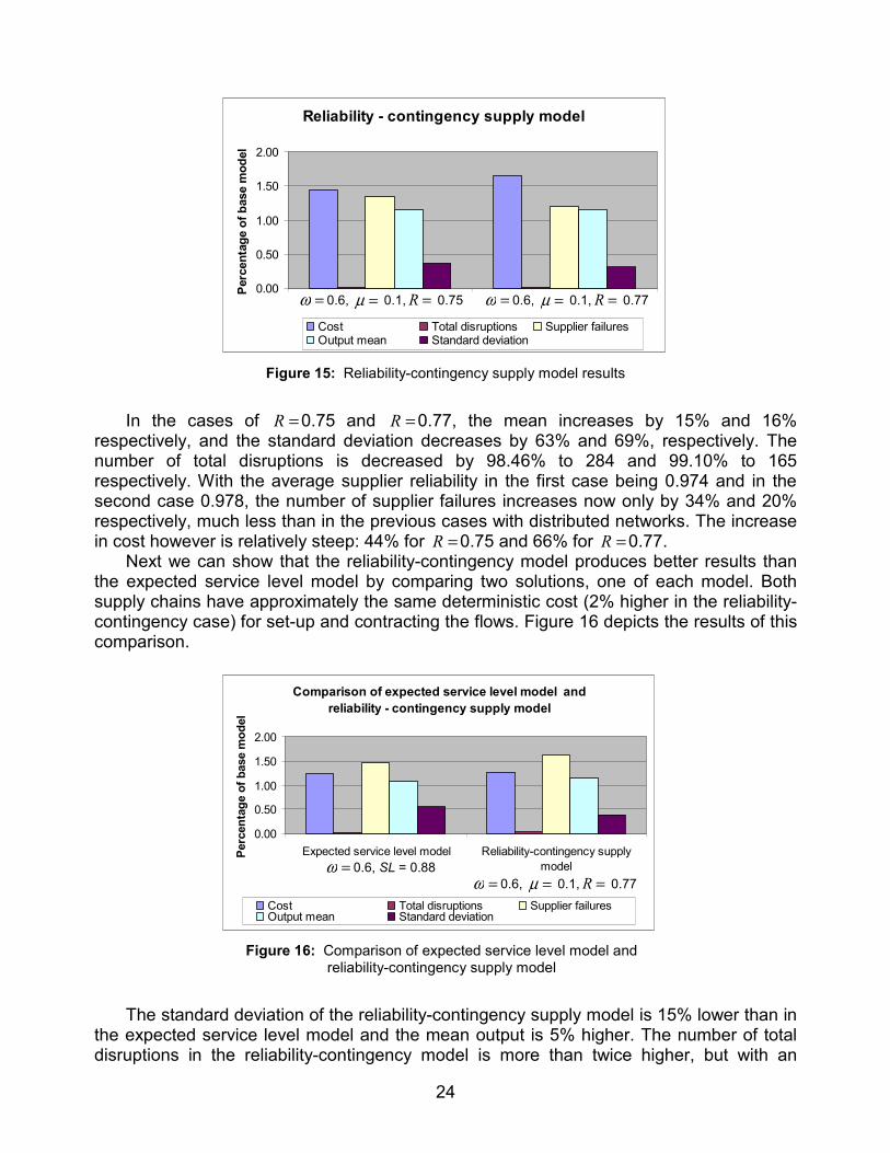
The best results in terms of reliability and robustness are obtained from the combination of the reliability and the contingency supply model. The reliability-contingency model produces the highest output mean, the lowest standard deviation, very few total disruptions and the highest supply chain reliability for distributed (non-serial) networks. Figure 14 depicts the supply chain for a sourcing limit of =ω 0.60, a maximum tolerated loss percentage of =µ 0.1 and a target supply chain reliability of =R 0.77.

Figure 14: Reliability-contingency supply model supply chain

In Figure 15 we give the results for two instances of this type of model: the one already

mentioned above and one with the same sourcing limit, same maximum tolerated loss percentage, but a target supply chain reliability of =R 0.75.

Stage 1 Stage 2 Stage 3 Stage 4 Stage 5

Europe

South-America

Stage 6

South-East-Asia

North America

=ω 0.6, =µ 0.1 =ω 0.6,SL = 0.9

24

Reliability - contingency supply model

0.00

0.50

1.00

1.50

2.00

Perc

enta

ge o

f bas

e m

odel

Cost Total disruptions Supplier failuresOutput mean Standard deviation

Figure 15: Reliability-contingency supply model results

In the cases of =R 0.75 and =R 0.77, the mean increases by 15% and 16%

respectively, and the standard deviation decreases by 63% and 69%, respectively. The number of total disruptions is decreased by 98.46% to 284 and 99.10% to 165 respectively. With the average supplier reliability in the first case being 0.974 and in the second case 0.978, the number of supplier failures increases now only by 34% and 20% respectively, much less than in the previous cases with distributed networks. The increase in cost however is relatively steep: 44% for =R 0.75 and 66% for =R 0.77.

Next we can show that the reliability-contingency model produces better results than the expected service level model by comparing two solutions, one of each model. Both supply chains have approximately the same deterministic cost (2% higher in the reliability-contingency case) for set-up and contracting the flows. Figure 16 depicts the results of this comparison.

Comparison of expected service level model and

reliability - contingency supply model

0.00

0.50

1.00

1.50

2.00

Expected service level model Reliability-contingency supplymodel

Perc

enta

ge o

f bas

e m

odel

Cost Total disruptions Supplier failuresOutput mean Standard deviation

Figure 16: Comparison of expected service level model and

reliability-contingency supply model

The standard deviation of the reliability-contingency supply model is 15% lower than in

the expected service level model and the mean output is 5% higher. The number of total disruptions in the reliability-contingency model is more than twice higher, but with an

=ω 0.6, =µ 0.1, =R 0.75 =ω 0.6, =µ 0.1, =R 0.77

=ω 0.6, =µ 0.1, =R 0.77 =ω 0.6, SL = 0.88

25

empirical probability of 0.45% it is still sufficiently low. The number of supplier failures is 16% higher in the case of the reliability-contingency model. We conclude that the most promising model in terms of reliability and robustness is the reliability-contingency model.

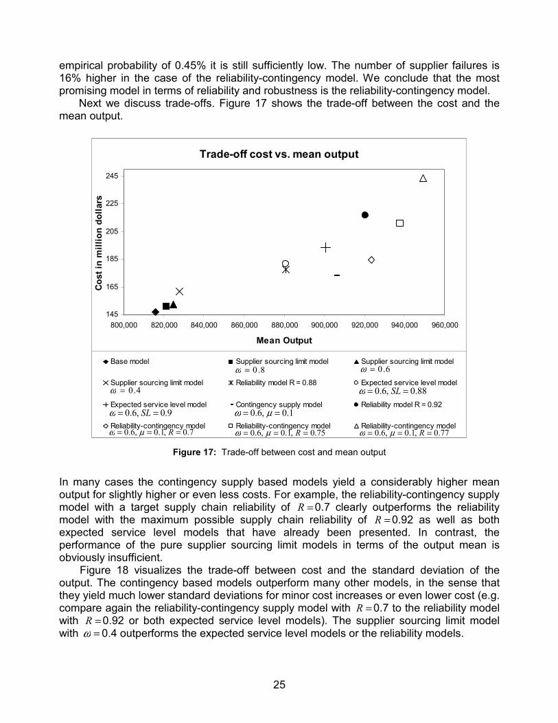
Next we discuss trade-offs. Figure 17 shows the trade-off between the cost and the mean output.

Trade-off cost vs. mean output

145

165

185

205

225

245

800,000 820,000 840,000 860,000 880,000 900,000 920,000 940,000 960,000

Mean Output

Cost

in m

illio

n do

llars

Base model Supplier sourcing limit model Supplier sourcing limit model

Supplier sourcing limit model Reliability model R = 0.88 Expected service level model

Expected service level model Contingency supply model Reliability model R = 0.92

Reliability-contingency model Reliability-contingency model Reliability-contingency model

Figure 17: Trade-off between cost and mean output

In many cases the contingency supply based models yield a considerably higher mean output for slightly higher or even less costs. For example, the reliability-contingency supply model with a target supply chain reliability of =R 0.7 clearly outperforms the reliability model with the maximum possible supply chain reliability of =R 0.92 as well as both expected service level models that have already been presented. In contrast, the performance of the pure supplier sourcing limit models in terms of the output mean is obviously insufficient.

Figure 18 visualizes the trade-off between cost and the standard deviation of the output. The contingency based models outperform many other models, in the sense that they yield much lower standard deviations for minor cost increases or even lower cost (e.g. compare again the reliability-contingency supply model with =R 0.7 to the reliability model with =R 0.92 or both expected service level models). The supplier sourcing limit model with =ω 0.4 outperforms the expected service level models or the reliability models.

4.0=ω

8.0=ω 6.0=ω

1.0,6.0 == µω

7.0,1.0,6.0 === Rµω

75.0,1.0,6.0 === Rµω 77.0,1.0,6.0 === Rµω

88.0,6.0 == SLω

9.0,6.0 == SLω

26

Trade-off cost vs. standard deviation

145

165

185

205

225

245

100,000 150,000 200,000 250,000 300,000 350,000 400,000

Standard deviation

Cost

in m

illio

n do

llars

Base model Supplier sourcing limit model Supplier sourcing limit model

Supplier sourcing limit model Reliability model R = 0.88 Expected service level model

Expected service level model Contingency supply model Reliability model R = 0.92

Reliability-Contingency model Reliability-Contingency model Reliability-Contingency model

Figure 18: Trade-off cost vs. standard deviation

Considering the trade-off between cost and total supply chain disruptions, we showed

that with all models, except the pure reliability models, large reductions in the number of total disruptions can be achieved.

To further validate our approach, the combined reliability-robustness models are tested on a second supply chain design instance with a different data set and they are again evaluated with respect to the results of the base model for this case. This second supply chain example consists of 33 nodes, which are distributed over the same four geographical regions, but with 5 stages ( =k 5). The final manufacturer is still located in North-America. In the supply chain figures that follow, a diamond represents a supplier and the hexagon the manufacturer. Like the previous instance, every stage except the last one has eight suppliers. However, the distribution of the suppliers on a stage over the geographical regions differs from the first example as do the values of most parameters. While the demand is still =D 1,000,000 units, the average supplier reliabilities of the more and the less reliable regions are higher than those in the first instance and the difference between the average reliabilities is now lower. For the more reliable regions it is

=avgr 0.986 and for the less reliable regions =avgr 0.973. The difference in the average production costs on the other hand is now greater. For North-America/Europe they are

=avgc $36.75 and for South-America/South-East Asia =avgc $19.3. With == ff e $220,000 the fixed costs in this instance are higher whereas the minimum flow requirements per arc

4.0=ω

8.0=ω 6.0=ω

1.0,6.0 == µω

7.0,1.0,6.0 === Rµω

75.0,1.0,6.0 === Rµω 77.0,1.0,6.0 === Rµω

88.0,6.0 == SLω

9.0,6.0 == SLω

27

of == qqe 70,000 units are the same as those in the first instance. Capacity limits are again not considered. The bill-of-materials parameters are assumed to be one.

The breakpoints of the staircase cost function for every arc are e : ea ,1 = 10,000 units,

ea ,2 = 125,000 units and ea ,2 = 275,000 units. The corresponding cost parameters, with respect to the production cost ecp along the respective arcs are ee cpcp =,1 , ecp ,2 =1.08 ecp⋅ and ecp ,3 =1.20 ecp⋅ .

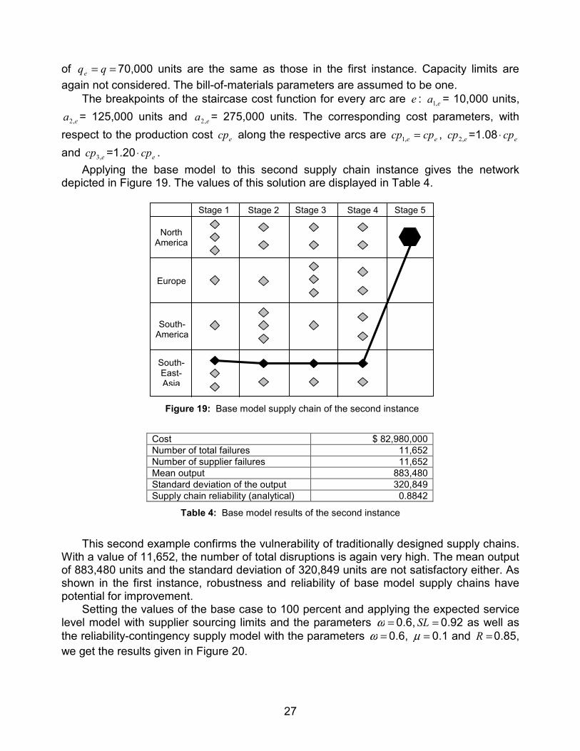
Applying the base model to this second supply chain instance gives the network depicted in Figure 19. The values of this solution are displayed in Table 4.

Figure 19: Base model supply chain of the second instance

Cost $ 82,980,000 Number of total failures 11,652 Number of supplier failures 11,652 Mean output 883,480 Standard deviation of the output 320,849 Supply chain reliability (analytical) 0.8842

Table 4: Base model results of the second instance

This second example confirms the vulnerability of traditionally designed supply chains.

With a value of 11,652, the number of total disruptions is again very high. The mean output of 883,480 units and the standard deviation of 320,849 units are not satisfactory either. As shown in the first instance, robustness and reliability of base model supply chains have potential for improvement.

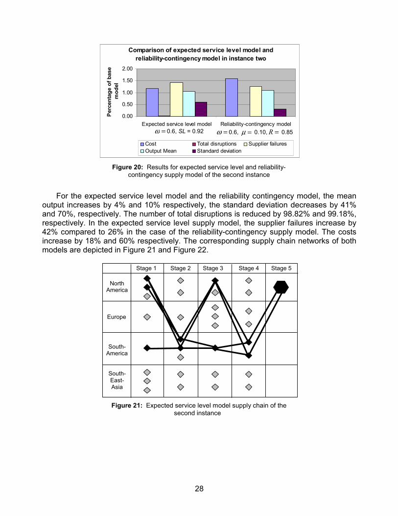
Setting the values of the base case to 100 percent and applying the expected service level model with supplier sourcing limits and the parameters =ω 0.6, =SL 0.92 as well as the reliability-contingency supply model with the parameters =ω 0.6, =µ 0.1 and =R 0.85, we get the results given in Figure 20.

Stage 1 Stage 2 Stage 3 Stage 4 Stage 5

South-East-Asia

North America

Europe

South-America

28

Comparison of expected service level model and reliability-contingency model in instance two

0.00

0.50

1.00

1.50

2.00

Exp del

Perc

enta

ge o

f bas

e m

odel

Cost Total dOutput Mean Standa

Figure 20: Results for expected secontingency supply model of

For the expected service level model and th

output increases by 4% and 10% respectively, thand 70%, respectively. The number of total disruprespectively. In the expected service level supply42% compared to 26% in the case of the reliabiincrease by 18% and 60% respectively. The corrmodels are depicted in Figure 21 and Figure 22.

Figure 21: Expected service level second instan

Stage 1 Stage 2 Sta

South-East-Asia

North America

Europe

South-America

Reliability-contingency model=ω 0.6, =µ 0.10, =R 0.85

ected service level mo=ω 0.6, SL = 0.92

isruptions Supplier failuresrd deviation

rvice level and reliability-

the second instance

e reliability contingency model, the mean e standard deviation decreases by 41% tions is reduced by 98.82% and 99.18%, model, the supplier failures increase by lity-contingency supply model. The costs esponding supply chain networks of both

model supply chain of the ce

ge 3 Stage 4 Stage 5

29

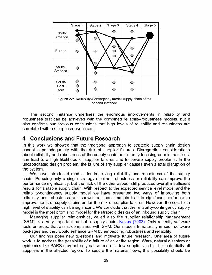
Figure 22: Reliability-Contingency model supply chain of the

second instance

The second instance underlines the enormous improvements in reliability and

robustness that can be achieved with the combined reliability-robustness models, but it also confirms our previous conclusions that high levels of reliability and robustness are correlated with a steep increase in cost.

4 Conclusions and Future Research In this work we showed that the traditional approach to strategic supply chain design cannot cope adequately with the risk of supplier failures. Disregarding considerations about reliability and robustness of the supply chain and merely focusing on minimum cost can lead to a high likelihood of supplier failures and to severe supply problems. In the uncapacitated design problem, the failure of any supplier causes even a total disruption of the system.

We have introduced models for improving reliability and robustness of the supply chain. Pursuing only a single strategy of either robustness or reliability can improve the performance significantly, but the lack of the other aspect still produces overall insufficient results for a stable supply chain. With respect to the expected service level model and the reliability-contingency supply model we have presented two ways of improving both reliability and robustness and shown that these models lead to significant performance improvements of supply chains under the risk of supplier failures. However, the cost for a high level of stability can be significant. We conclude that the reliability-contingency supply model is the most promising model for the strategic design of an inbound supply chain.

Managing supplier relationships, called also the supplier relationship management (SRM), is a very important part of a supply chain, Navas (2003). Only recently software tools emerged that assist companies with SRM. Our models fit naturally in such software packages and they would enhance SRM by embedding robustness and reliability.

Our findings pose new questions and motivate future research. One area of future work is to address the possibility of a failure of an entire region. Wars, natural disasters or epidemics like SARS may not only cause one or a few suppliers to fail, but potentially all suppliers in the affected region. To secure the material flows, this possibility should be

Stage 1 Stage 2 Stage 3 Stage 4 Stage 5

South-East-Asia

North America

Europe

South-America

30

accounted for as well. We propose an alternative formulation for calculating the supply chain reliability that considers regional reliabilities as well. Let G be the set of all regions. Let jr~ denote the reliability of region j and let jZ

~ be a binary variable indicating if the supply chain has suppliers in region j . Then, the equation for supply chain reliability (1) can be stated as

{ }

∏∏∈∈

⋅=Gj

Zj

nNv

Zv

jv rrR~

/

~~ . ( 42 )

We can linearize (42) by applying logarithms on both sides. New linear constraints have to be added that model the definition of jZ

~ . To improve robustness of a supply chain in the case of an entire region failing, we can

extend the idea of supplier sourcing limits to regional sourcing limits. In this case, a customer node can only source a given percentage τ of its total supply from the suppliers in a particular region. For Nv∈ , Gj∈ let AI jv ⊆~ be the set of incoming arcs from region j to node v . We can express the regional sourcing limits as

∑∑∈∈

⋅≤vjv Ie

eI~e

e XX τ for all Uk

iiSv

2=

∈ .

In our work we have shown the trade-offs between the cost on the one side and reliability/robustness on the other. The decision, which model to use for a particular supply chain problem depends on a given context. First, on the type of product the inbound supply chain is designed for. Profit, strategic importance to the manufacturer or vital necessity of a product, e.g. in the case of pharmaceutical products, have a major influence on how reliable and robust a supply chain is desired to be. The market position of the manufacturer is another influencing factor. In highly competitive environments, where excess demand usually cannot be back-ordered but is lost, robustness and reliability play a more important role than in monopolies. A third, major factor is the attitude of the management towards risk. Therefore, another future direction is the deployment of multi-attribute utility theory to propose a way of finding the best solution for a specific case in terms of the various trade-offs and reflecting the risk preferences of the management.

Our assumption is that a supplier ships either all or none of the required supply. An extension would be to consider the probability distribution for providing a certain percentage of supply.

Another logical step is to move from the strategic to the tactical planning level and to incorporate aspects of reliability and robustness in multi-period inventory models.

References AMPL. Available at: http://www.ampl.com. ANDREWS, J. D. and MOSS, T. R. 2002. Reliability and Risk Assessment. ASME Press.

New York. AXSÄTER, S. 1993. Continuous Review Policies for Multi-Level Inventory Systems with

Stochastic Demand. In: Graves, S. C., Rinnooy Kan, A. H., Zipkin, P. H., (Eds). Logistics of Production and Inventory. North-Holland Publishing Company, Amsterdam.

31

BUNDSCHUH, M. 2003. Modeling Robust and Reliable Supply Chains. Studienarbeit at

Fachgebiet Fertigungs- und Materialwirtschaft, Darmstadt University of Technology, Germany.

DAVIS, T. 1993. Effective Supply Chain Management. Sloan Management Review,

Summer 1993, 35-46. DIKS, E. B., DE KOK, A. G. and LAGODIMOS, A. G. 1996. Multi-Echelon Systems: A

Service Measure Perspective. European Journal of Operational Research, 95, 241-263. FEDERGRUEN, A. 1993. Centralized Planning Models for Multi-echelon Inventory

Systems under Uncertainty. In: Graves, S. C., Rinnooy Kan, A. H. and Zipkin, P. H., (Eds). Logistics of Production and Inventory. North-Holland Publishing Company, Amsterdam.

FORRESTER, J. 1961. Industrial Dynamics. MIT Press, Cambridge. GOETSCHALCKX, M. 2000. Strategic Network Planning. In: Stadtler, H. and Kilger, C.,

(Eds.). Supply Chain Management and Advanced Planning: Concepts, Models, Software and Case Studies. Springer, Berlin. 79-95.

HODDER, J. E. and DINCER, M. C. 1986. A Multifactor Model for International Plant

Location and Financing under Uncertainty. Computers & Operations Research, 13, 601-609.

HUCHZERMEIER, A. 1991. Global Manufacturing Strategy Planning under Exchange

Rate Uncertainty. Ph.D. Dissertation, Decision Sciences Department, Wharton School, University of Pennsylvania, Philadelphia.

HUCHZERMEIER, A. and COHEN, M. A. 1996. Valuing Operational Flexibility under

Exchange Rate Uncertainty. Operations Research, 44, 100-113. ILOG CPLEX 8.0. 2002. User’s Manual. INDEFURTH, K. 1994. Safety Stocks in Multistage, Divergent Inventory Systems: A

Survey. International Journal of Production Economics, 35, 321-329. KUO W. and ZUO, M. J. 2003. Optimal Reliability Modeling: Principles and Applications.

John Wiley & Sons, Hoboken. LEE, H. L., PADMANABHAN, P. and WHANG, S. 1997. The Bullwhip Effect in Supply

Chains. Sloan Management Review, Spring 1997, 93-102. MARTHA, J. and VRATIMOS, E. 2002. Creating a Just-in-Case Supply Chain for the

Inevitable Next Disaster. Marsh & McLennan Companies Report. Available at: http://www.mmc.com/views2/autumn02Martha.php.

NAHMIAS, S. 2001. Production and Operations Analysis. McGraw-Hill, Boston.

32

NAVAS, D. 2003. SRM: Where Co-dependency Succeeds. Supply Chain Systems Magazine, 23, 20-27.

NAVAS, D. 2003a. Automotive Embraces Volatility. Supply Chain Systems Magazine, 23,

12-16. SANTA-FE INSTITUTE. 2001. Working Definitions of Robustness. Internal report RS-

2001-009. Available at: http://discuss.santafe.edu/robustness/stories/storyReader$9. SCHWARZ, L. B. 1989. A Model for Assessing the Value of Warehouse Risk-Pooling:

Risk-Pooling over Outside-Supplier Leadtimes. Management Science, 35, 828-842. SCHWARZ, L. B. and WENG, Z. K. 2000. The Design of a JIT Supply Chain: The Effect of

Leadtime Uncertainty on Safety Stock. Journal of Business Logistics, 21, 231-253. SHEFFI, Y. 2001. Supply Chain Management under the Threat of International Terrorism. The International Journal of Logistics Management, 12, 1-11. SNYDER, L. V. and DASKIN, M. S. 2003. A Reliability Model for Facility Location.

Presentation at the INFORMS workshop on “Managing Risk in an Uncertain World”. Northwestern University, Evanston.

SONI, S. and PIRKUL, H. 2002. Design of Survivable Networks with Connectivity

Requirements. Telecommunication Systems, 20, 133-149. VAN DER FORST, J. G. A. J., BEULENS, A. J. M., DE WIT, W. and VAN BEEK, P. 1998.

Supply Chain Management in Food Chains: Improving Performance by Reducing Uncertainty. International Transactions in Operational Research, 5, 487-499.

VAN HOUTUM, G. J., INDERFURTH, K. and ZIJM, W. H. J. 1996. Materials Coordination

in Stochastic Multi-echelon Systems. European Journal of Operational Research, 95, 1-23.

VAN LANDEGHEM, H. and VANMAELE, H. 2002. Robust Planning: A New Paradigm for

Demand Chain Planning. Journal of Operations Management, 20, 769-783. VIDAL, C. J. and GOETSCHALCKX, M. 2000. Modeling the Effect of Uncertainties on

Global Logistics Systems. Journal of Business Logistics, 21, 95-120. VIDAL, C. J. and GOETSCHALCKX, M. 1997. Strategic Production-Distribution Models: A

Critical Review with Emphasis on Global Supply Chain Models. European Journal of Operational Research, 98, 1-18.