The Impact of Military Forts on Agricultural Investments on the ...

University of Nebraska - Lincoln University of Nebraska - Lincoln

DigitalCommons@University of Nebraska - Lincoln DigitalCommons@University of Nebraska - Lincoln

Center for Great Plains Studies: Staff and Fellows Publications Great Plains Studies, Center for

2009

The Impact of Military Forts on Agricultural Investments on the The Impact of Military Forts on Agricultural Investments on the

Great Plains in 1880 Great Plains in 1880

Christopher S. Decker University of Nebraska at Omaha, [email protected]

David T. Flynn University of North Dakota, [email protected]

Follow this and additional works at: https://digitalcommons.unl.edu/greatplainsfellows

Part of the Other International and Area Studies Commons

Decker, Christopher S. and Flynn, David T., "The Impact of Military Forts on Agricultural Investments on the Great Plains in 1880" (2009). Center for Great Plains Studies: Staff and Fellows Publications. 1. https://digitalcommons.unl.edu/greatplainsfellows/1

This Article is brought to you for free and open access by the Great Plains Studies, Center for at DigitalCommons@University of Nebraska - Lincoln. It has been accepted for inclusion in Center for Great Plains Studies: Staff and Fellows Publications by an authorized administrator of DigitalCommons@University of Nebraska - Lincoln.

The Impact of Military Forts on Agricultural Investments on the Great Plains in 1880

by

Christopher S. Decker and David T. Flynn Department of Economics Department of Economics College of Business Administration College of Business & Public University of Nebraska at Omaha Administration Omaha, NE 68164 University of North Dakota and Grand Forks, ND 58202 Research Fellow Center for Great Plains Studies University of Nebraska at Lincoln Lincoln, NE 68588

Abstract

We empirically investigate the relationship between agricultural development and proximity to military forts in Kansas, Nebraska, and Colorado in 1880. Agricultural investments are substantially higher in counties where a military fort is present, suggesting that military forts stimulated agricultural development on the Great Plains. However, the reverse is not true; there is no statistical support for the notion that forts necessarily located in counties where substantial development was already occurring. Moreover, we found that while the presence of a military fort has the effect of increasing agricultural development, there is no evidence that such a presence sustained agricultural development. Keywords: Forts, Great Plains, Agriculture JEL Codes: N51, N91, R11, R53

1

Abstract

We empirically investigate the relationship between agricultural development and

proximity to military forts in Kansas, Nebraska, and Colorado in 1880.

Agricultural investments are substantially higher in counties where a military fort

is present, suggesting that military forts stimulated agricultural development on

the Great Plains. However, the reverse is not true; there is no statistical support

for the notion that forts necessarily located in counties where substantial

development was already occurring. Moreover, we found that while the presence

of a military fort has the effect of increasing agricultural development, there is no

evidence that such a presence sustained agricultural development.

Keywords: Forts, Great Plains, Agriculture JEL Codes: N51, N91, R11, R53

I. Introduction

The role of government in fostering economic growth is a contentious

issue in contemporary economic development as well as the historical

development of the United States and its various regions. For instance, consensus

generally supports the notion that state and local taxation acts as a drag on

economic growth (Becsi, 1996). However, investment in public infrastructure

2

financed through taxes and bond issuance tends to generally support private sector

growth (Chandra and Thompson, 2000).

From a historical perspective, there are additional examples of private

sector benefits of governmental investments. Craft (1998) finds that government

installation of weather reporting stations on coastal areas around the Great Lakes

in the late nineteenth century reduced shipping accidents, though the success of

other nineteenth century policies is questionable. Lindert (1993) discussed

government subsidization as one of the major influences on farmland prices.

Notable among these are the various public land disposal policies of the era.

The Homestead Act of 1862 was designed to promote settlement and

agricultural investments on the American Frontier. Evidence recently published

by Stewart (2006) shows substantial wealth accumulation in Kansas, Nebraska,

and the Dakotas in the 1860s and 1870s attributable to the Homestead Act.

However, general consensus is the policy, as well as other subsequent land

disposal acts, was largely a failure, particularly in the western and northern Great

Plains. This failure was due largely to the fact that the provisions in the policy

(offering 160 acres to settlers free with the promise of a five year tenure and land

improvement efforts) attracted an unsustainably large number of small, asset-

limited, farmers to the region (Hanson and Libecap, 2003). While there was

evidence some farm operations were successful for a time, during periods of

severe drought, crop yields fell and incomes plummeted. Moreover, the farms

3

themselves were too small to exploit scale economies and other advantages from

large scale operations that would help them sustain operations in such an arid

region (Libecap and Hansen, 2002). Olson and Naugle (1997, p. 160) document

that in Nebraska, of the 131,561 persons who filed homestead entries in 1862,

only 68,862 received final patents in 1900. Fully 48 percent of all homestead

operations in Nebraska failed by 1900 and many of these were in the western part

of the state, west of the 98th meridian where annual precipitation falls off

dramatically (Webb, 1931).

While the evidence is fairly clear, particularly in the arid western regions

of the Great Plains, governmental efforts to transfer public land to smaller, private

concerns failed to foster sustained economic enterprise, there are some examples

that would appear to run counter to this trend. According to the Tenth Decennial

Census of the United States 1880: Volume III: Report on the Production of

Agriculture, average land values for Nebraska and Kansas counties east of the 98th

meridian was about $12.00 per acre. Moreover the average share of improved

acreage to total was 56.5 percent. However, in Arapahoe County in Colorado,

land sold for over $15 per acre with roughly 32 percent of the county’s acreage

experiencing capital improvements. Moreover, in Lincoln County, Nebraska,

another county west of the 98th meridian, 78 percent of the land was subject to

improvements and land there was valued at $8.56 per acre. Finally, in Costilla

County, Colorado, 72 percent of the land was subject to improvements, indicating

4

a substantial amount of agricultural investment. While land there was valued at

$4.74 per acre, this rate was substantially larger than the average land value in six

eastern Kansas and Nebraska counties, such as Cheyenne County, Kansas where

land was valued at $2.17 per acre.

There are several possible reasons for why these arid counties appeared to

have experienced some relative success. Both Arapaho County, Colorado and

Lincoln County, Nebraska benefited from railroad access as well as river access

for cultivation and irrigation. However, neither a substantial river nor railroad

was present in Costilla County, Colorado in 1880. There were no major

population centers to support demand for agricultural goods either. It is perhaps

quite telling, however, that Fort Garland operated in this county between 1853

and 1883.

In this paper, we address the role the frontier army played in the

development of the American West, specifically as it relates to agricultural

investment, the primary motivation behind the Homestead Act of 1862 and many

subsequent US land policies. There are at least three reasons why proximity to

military forts on the frontier would offer and incentive for farmers to invest in

land improvement activities.1 Soldiers and fort personnel in general represented a

1 As Dobak (1998, p. 7) points out, most histories of the frontier army’s role in the American West “ignores relations between military posts and the surrounding communities: whether the army and the market it afforded helped attract settlers; or who got the army’s money, how they spent it, and how that affected the community.” As we hope to document in this paper, both the historical

5

source of demand for local agricultural output. The historical record is replete

with stories of local communities benefitting from military expenditures on

locally available provisions and food stuffs as well as indirect benefits of skilled

brought to satisfy fort demands (Freedom, 1976, 97). In his extensive history of

Fort Riley, Kansas, Dobak (1998, p. 5) documents how farmers located near the

fort were elated by the arrival of substantial cavalry companies in 1880 as it

meant increased demand for hay and feed grain for companies’ horses. West

(1998, p. 276) writes that “troops were consumers – in their case especially

voracious ones – of the vituals around them.” (p. 276). He further added that

local “enterprises quickly struck up a dynamic give-and-take with the posts.

Freedom (1976, p. 82) suggests significant buying from local area producers

occurred after the local population and transportation network developed

sufficiently. Road stores catered to the soldiers’ daily needs and vices and also

supplied emigrants and travelers moving west. The soldiers and fort represented

the retail market for local stores. Early ranchers found a market for their cattle,

farmers for their grains, pumpkins, cabbages, onions, and other produce.” (p.

276). Such relationships were quite lucrative prospects for local farmers indeed.

In his extensive study of the role the frontier army played in the development of

the American West, Tate (1999, p. 119) indicates one of the most lucrative

military contracts was for the supply and delivery of beef, mutton, and other food record and the supporting statistical analysis show that the activities of the frontier army did have a substantial role to play in the frontier economy of the nineteenth century.

6

stuffs to military posts. According to Tate these contracts were second in value

only to larger construction project contracts.2 To the extent, then, that the

presence of a nearby military fort stimulated demand for agricultural goods,

farmers located in these areas had incentives to increase production to meet this

demand and possibly secure military contracts, creating an incentive for

increased land improvement activities. Until local activity reached sufficient scale

fort needs were met by producers from outside the immediate region (Freedom,

1976, p. 85).

Many soldiers also engaged in limited agricultural activities on military

posts. Tate (2007, p. 51-54) describes instances of military personnel extensively

experimenting with novel agricultural techniques including dry land farming.

Freedom (1987) documented many army writings about trial-and-error planting

and harvesting techniques ultimately published, booster newspapers and other

periodicals that were distributed in the Eastern United States and Europe to attract

settlement. Robinson (1977) points out that gardening was indeed encouraged at

forts and that soldiers engaged in such activities disseminated their experiences

through libraries and reading rooms. Forts also enhanced access to

2 The impact of a military presence on a local economy is certainly not limited to the nineteenth century American West. Other historical examples include Dunn, Jr. (2002) documenting the critical role the British Army played in private enterprise development after the end of the French and Indian war in 1763. Moreover, it has been demonstrated that rural contemporary economies in the United States are adversely affected by the closing of a nearby military bases, although there is debate as to the long term magnitude of such impacts on local communities (see, e.g. Hooker and Knetter, 2001).

7

communication sources such as mail and the telegraph. Freedom (1976)

identified agicultural knowledge as the significant contribution of military

agriculture in the settlement of the northern Plains. Dobak (1998, p. 61, 63) also

offers examples of military personnel remaining in settlements near the forts

where they were stationed after their terms of enlistment ended to take up many

vocations, including private farming activities. One might expect increased

investment activities in areas near forts where successful and novel cultivation

activities were proven beneficial and where additional private farming activities

took place by retiring army personnel.

Finally, a military presence likely encouraged investment by deterring

farm property pilfering and destruction by Indian raiders attempting to prevent

white settler encroachment on their land or outlaw bandits. As Hart (1963, p.

118) describes, “Regardless of where they were, or why, the citizens of nineteenth

century America felt the deserved protection from the Army.” Freedom (1987)

documents several instances where several forts were established in the Dakota

Territories largely to protect white settlements.3

The economic history of the American west is largely a story of public

land disposal, westward migration, and, importantly, the establishment and

3 For example, according to Freedom (1987), Fort Dakota, near present day Sioux Falls, South Dakota and Fort Ellis near Bozeman, Montana were established largely to protect settlement in those regions. While these areas are outside our study area due to the fact that neither the Dakotas nor Montana were states and thus we have no county level data for the period of focus here, these examples highlight the importance of frontier forts as protectors.

8

enforcement of private property rights, a stark contrast with the economic history

of the American east (Anderson and Hill, 1975, 1990; Anderson and Leal, 1991).

A focus on property right protection is therefore germane. Secure property rights

increase individual incentives to invest in innovation and production because of

the reduced dissipation of economic rents through theft, arbitrary confiscation,

contractual holdup, or other rent-seeking activities (North;1987, 1990). Many

studies support the idea that secure and enforceable property rights, whether

governmental or privately developed institutions, promote economic growth

(Thorstensson, 1994; Domcer, 2007) and investment, both internationally (Besley,

1995), and within the context of the nineteenth century American west (Anderson

and Hill, 2004, p. 22; Kanazawa, 2006).

The role of the frontier army as protectors of private property, however, is

not immediately obvious. It does appear to be the case that a number of military

forts, such as Fort Kearny in Nebraska, were established to protect emigrants

moving west along the Platte River road from Indian raids, outlaws, etc. (Frazier,

1988, p. 87). That said, the task of establishing federal policing powers without

encroaching on citizens’ civil liberties has pre-occupied legislators and policy

makers since the inception of the United States. The Judiciary Act of 1789 was

the first attempt to delineate the relationship between local marshals and federal

enforcement of law. With respect to the nineteenth century American west, the

1878 amendment to that year’s military appropriations act advanced by

9

Representative William Kimmel of Maryland severely restricted military

involvement in civil enforcement and established penalties for military personnel

who stepped beyond the delineations established by the act.4 These restrictions

were not without controversy. In 1871 Secretary of War William Belknap cited

many examples of how soldiers had coordinated with local law enforcement to

make arrests, detain prisoners, prevent thievery, etc. (Tate, 1999, p. 3). Indeed,

speaking of military officers’ attitudes towards their delineated federal powers to

intervene in civil affairs, Tate (1999) describes:

At times, the majority preferred a loose interpretation of that power, thus allowing them to arrest and hold small numbers of outlaws and rioters for short periods of time. They well recognized that the more remote areas of the West lacked sufficient civilian law enforcement personnel to deal with some of these problems. Even under the threat of possible legal reprisal for arresting civilians, most military officers carried out their duties with dedication.” (p. 110).

In short, one would expect a military presence could reasonably be seen as a

source of civil protection, at least for transportation routes, thereby reducing the

threat of rent dissipation and fostering investment activities.

While the three reasons detailed support the notion that establishment of

military installations in the American west tends to support economic growth and

investment, it could be that such establishments hindered local and regional

growth and investment, particularly in agriculture. Dobak (1998, p. 1977)

4 In effect, the act restricted military action to exceptional cases of insurrection or riot, the endangerment of public (not private) property, and efforts to disrupt federal mail service.

10

articulates this view well by pointing out that the military did sequester acres of

land for military purposes, closing many areas to settlement and homesteading

and limiting the tax base for local government. These activities likely had a

detrimental impact on private sector activities.

The opposing views make the question of the frontier army’s role in the

development of the west is an empirical one. The paper is organized as follows. In

sections II and III we describe the scope of the study, empirical model variables

and data sources. In section IV we address specifics element of the estimation

procedure. In section V we present the model results and in section VI we

conclude and offer avenues for future research.

II. Nature and Scope of Empirical Analysis

The empirical analysis conducted here uses county data mostly from tables

published in the Tenth Decennial Census of the United States of 1880 (Census),

compiled by the Inter-University Consortium for Political and Social Research

(ICPSR), and focuses on the region defined by the states of Kansas, Nebraska and

Eastern Colorado (about 179 total counties). Our dependent variable is the

proportion of improved county acreage, defined as ACIMP, obtained from the

Census. Since the historical census of the United States for 1880 does not appear

to have tracked a direct measure of agricultural investment, ACIMP serves as a

proxy for investment in that it measures acreage subject to improvement for

cultivation purposes, such as the clearing of brush and trees, leveling/landscaping

11

of land for growing crops, land tillage, irrigation networks, etc. Such activities

require a substantial amount of labor and capital investment. Hence, this variable

is a reasonable measure of the capital and labor investment effort undertaken by

homesteaders. If a military presence does indeed support property right protection

and afford a ready market for agricultural output, one would expect a greater

degree of such investment in those areas were a fort is located.5

As stated earlier, the empirical analysis conducted here focuses on the

region defined by the states of Kansas, Nebraska and Eastern Colorado. All three

were states by 1880 and therefore county level census data is available. There

appears to be substantial interest in the economic development of the American

mid-West and Plains region evidenced by recent scholarship (Cunfer, 2005;

Stewart, 2006). There may be several reasons for this interest. Prior to the

outbreak of the Civil War, this region was largely considered uninhabitable and of

little economic value. An early American explorer of the west, Stephen H. Long,

described this region as “wholly unfit for cultivation…by a people depending on

agriculture for their subsistence” and labeled the region “the Great American

5 It may also be reasonable to suggest farm land values as an alternative measure of the economic impact of a frontier fort in that one would expect such land to be of higher value as potential settlers and/or land speculators bid up land prices for these attractive tracts of land if a fort affords a readily accessible market for agricultural goods as well as property right protection.. However, given that it is equally reasonable to hypothesize that a military presence would stimulate investment in land improvements, and given that several recent studies, notably Craig, Palmquist and Weiss (1998) and Decker and Flynn (2007) have found evidence that land values are strongly linked to acres improved, we might encounter an endogeneity problem were we to focus on land values directly. As we will see, we do find evidence that proximity to military establishment do stimulate investment in land improvements. Hence, indirectly, our findings support the notion that such proximity will also stimulate land values.

12

Desert.”6 Beginning in the 1860s, this perception changed dramatically due to the

passage of the Homestead Act, improved farming technology and transportation

infrastructure, and increased efforts by “boosters”. This dramatic change in

perception resulted in an influx of citizens from the densely populated cities of the

east.

This region developed into an agricultural economy that became a major

contributor to the economic growth and development of the United States in the

late nineteenth and early twentieth centuries. The combination of rapid world

population growth and urbanization created substantial increases in world demand

for food products, notably wheat (White, 1993, p. 244). As a result wheat became

the major commodity in this region. In 1882, Kansas, Nebraska, and the Dakota

territories accounted for 12 percent of total wheat production in the United States.

By 1900, they accounted for 27 percent. By the second decade of the 20th

century, the United States, for the first time in its history, became a creditor

nation. While manufacturing and other sectors certainly played a role in this,

agriculture’s role in this favorable trade balance cannot be overlooked (Walton

and Rockoff, 1998, p. 460-61). This region has remained a major center of

agriculture to this day.

Finally, the focus on this region is advantageous from an econometric

perspective. Answering whether, and to what extent, forts impacted agricultural 6 This excerpt has been quoted much in American history. This quote was taken from Hine and Faragher (2000, 160).

13

investment requires that fort location be exogenous; that is, the presence of a

military establishment induces agricultural investments, not that fort sites were

selected in areas where land improvements have already taken place. The idea

that forts may have been largely built in places that could best serve pioneers

immigrating to westward to California or the Oregon Territories supports the

notion that settlement and agriculture in the mid-West and Plains region largely

followed after such fort installation reduces the potential for endogeneity. This

said, below we do test for this potential reverse causality econometrically below.

The time period selected is worth noting as well. After the end of the

Civil War, union army personnel were by-in-large redeployed to western regions

of the nation to support, among other things, westward migration and protect

settlers and capital (largely railroad and telegraph infrastructure) from Indian

raids. Most territories in the Plains region had not yet, or had only recently

achieved, statehood making reliable data from the 1860 and 1870 censuses largely

incomplete. From 1890 through 1900, it became clear the end of the Plains Indian

War was coming and many frontier military forts were being abandoned or

demolished as the US frontier army was largely re-deployed to the nation’s

coastal areas for more rapid deployment overseas.7 As a result, to detect any

potential link between economic development and agricultural development and 7 Also with the end of frontier hostilities, the army began to cut down on enlistments, not fill any vacant military positions in frontier regions, and consolidate military operations in a few remaining western forts. This last point is of potential interest as a future research directive since it is not readily clear what criteria was applied to select forts for closure and forts for consolidation.

14

the frontier Army, the 1880 period would offer the most reasonable time frame to

focus upon.

III. Model Variables and Data Sources

The incentives to invest in agricultural land improvements are determined

by the prevailing cost and demand considerations in the market for agricultural

goods. On the cost side, land better suited for agricultural development will

generate more efficient production and therefore offer homesteaders an

opportunity to produce more efficiently (cost-effectively) than land less well

suited for agricultural development. As a measure of the productive capacity of

land, we construct a variable, YLD, again using data from the Census, which

measures the ratio of bushels of agricultural crops produced to total acres planted

for each county.8 We would expect more investment in improved acres to be

associated with greater productive yield of the land. Moreover, easier access to

markets as well as sources of productive capital can generate efficiencies in

production. To address this, we include two variables. The first is a measure of

the ratio of manufacturing employment to total population in a given county,

MAN_EMP/POP, both taken from Census. Much of the manufacturing activities

of this period and region were operations that supported the capital needs of local

farmers, such as blacksmithing. The second variable, RR, indicates the presence

8 The agricultural products used in this calculation were barley, buckwheat, corn, oats, rye, and wheat. It should be noted that this variable could also be influenced by the acres improved variable, ACIMP, in that higher productivity is likely influenced by the degree of improvements to land. This potential endogeneity will likely bias our statistical result. Therefore, our econometric procedures will address this issue.

15

of a railroad line and is equal to one if the county in question contained a railroad

passing through it as of 1876. This data was generated by the authors from

detailed inspection of state maps in the year 1876 as published by Rand McNally

(see Table 1 for details). In both cases, we would expect greater improvements to

land due to more manufacturing activities and the presence of a rail line.

With respect to market demand incentives to invest in agriculture, we

include two population variables, POP/FARMS, and POPST/FARMST. The first

variable is the ratio of county population to total number of farms. We expect that

the greater the local demand for farm output (i.e. the greater the population

relative to producers), the more investment in agricultural production will take

place. It is also possible that some farm operations looked beyond the local

market (as defined by county delineation). To proxy for farms in a given county

having a wider market orientation we include the ratio of that population in a

given state net of the population in county i, to total farms in the state, net of

farms in a given county i. Again, we would expect a positive effect on

agricultural investment here as well.

As for the effect of proximity to a frontier army fort, we generated two

dummy variables, FORT, and NEARFORT. The FORT variable indicates the

presence of at least one operating military fort in a given county i in 1880. This

16

data was compiled from maps published in Hart (1963, 1964).9 In addition, we

constructed a variable NEARFORT which indicates, for a given county i, at least

one fort located in a county adjacent to that county. In both cases, if proximity to

a military fort stimulates agricultural investment, we would expect to see a

positive effect.

In addition, we also include two state dummy variables indicating Kansas

or Nebraska to capture state-specific elements that might otherwise be omitted by

other variables. Recalling that our dataset covers these states plus eastern

Colorado, it may be that there are certain state characteristics unique to each that

might support agricultural land development. For instance, the fact that in 1880

Kansas had more population centers and therefore achieved statehood before

Colorado may have given state legislators more time to influence agricultural

development relative to Colorado. Once the various data sources are linked

together, we end up with a 163 observations.

IV. Empirical Model Specification

9 Indeed, compiling this data was actually a bit more complicated. The maps published by Hart give a rough location of military forts and smaller military camps and the years in which these forts were in operation. Once those forts that were in operation in 1880 were identified, we conducted internet searches on each fort to pinpoint specific county location. At the time we also attempted to find data on garrison size in this period hypothesizing that not only proximity to a fort but the relative size of the military personnel present would also impact investment decisions. However, no such data was available either from individual internet sites nor from for sources, such as various government documents that addressed military budgets of the time. That said, we did take care to only include military forts and to exclude military posts, which as a rule tended to be smaller, of then with only one or two solders deployed at a given time and were more temporary in nature and construction.

17

When implementing our empirical model, we could have used standard

OLS, modeling the natural log of ACIMP as a function of the variables discussed

above. However, doing so does not take into account that ACIMP is essentially

bounded between zero and one since it is not possible to improved more acres in a

county than are present.10 Hence, the resulting estimators cannot be assured un-

biased and consistent. We therefore adopt a modeling procedure which explicitly

takes this characteristic into account.11 Specifically, we assume, as is commonly

done, ACIMP is a conditional probability that follows a logistical distribution.

Using the independent variables discussed above, we estimate the following

equation:

0 1 2

3 4

5 6 7

8 9

ln ln( ) ln( / )1

ln( / ) ln( _ / )1876

,

⎛ ⎞= + +⎜ ⎟−⎝ ⎠+ +

+ + ++ + +

ii i i

i

i i i i

i i i

i

ACIMP YLD POP FARMSACIMP

POPST FARMST MAN EMP POPRR FORT NEARFORTDMYNE DMYKS e

β β β

β ββ β ββ β

(1)

10 A reasonable alternative specification may have been to model acres improved as a function of total acres plus the additional variables described above. This, however generated some statistical problems as total acres is highly correlated with some other model variables, such as population and agricultural yields. This potential multicollinearity could significantly bias our resulting standard errors. Modeling ACIMP as we have mitigates multicollinearity concerns (see Table 2). 11 The procedure employed here comes largely from Greene (1993, p. 653-654) who provides a detailed background on the application of regression analysis to proportional data.

18

where we use the log-form of our continuous independent variables. This was

done because this specification generated the most desirable statistics.12

Under the logistic distribution assumption, so long as ACIMP lies between

0 and 1, as is the case in our dataset, equation (1) can be estimated via OLS.13 The

main econometric problem remaining, however, is that the variance of the

resulting estimated residuals from such a regression are, by construction,

heteroscedastic. To correct for this, we follow procedures detailed in Greene

(1993, p. 654) and first estimate our model via OLS to obtain consistent estimates

of the model parameters. The fitted equation is then used to construct weights

that correct the heteroscedasticity problem.14 Equation (1) is then re-estimated via

weighted least squares, the results of which are presented in Table 3.

12 This also had the added benefit of allowing the resulting coefficients on our continuously-defined variables to be interpreted, with some minor modification, as elasticities. To be sure, there are other legitimate functional forms that could have been estimated. Indeed, we investigated anther common form, the semi-log functional form whereby our continuous independent variables were included. This model produced higher regression errors and other less-desirable model statistics. Hence, we opt to focus on the log-linear form here. Results from this alternative specification are available upon request from the authors. 13 To see this, let y=LOSS/TONS. Then if y, conditioned on model variables, x, follows the

logistic distribution, exp(x ' )y1 exp(x ' )

β=

+ β. After some algebra, we have yln x '

1 y⎛ ⎞

= β⎜ ⎟−⎝ ⎠.

14 For the Logistic model, the error term iε is heteroscedastic with a variance equal to 1( )

(1 )=

Λ −Λi iVar

nε where Λ is the ACIMP and nt is the number of “trials” in county i. Notice

the source of the heteroscedasticity in that the variance is not constant but rather changes with ACIMP. Hence, the weights used to estimate (1) are ( )1= Λ −Λi i i iw n . Since Λi is not known, we adopt the following two step procedure where we first estimate (1) via OLS and then calculate the fitted values of ACIMP: Λi , which are used to construct wt and then used to re-estimate (1). The number of “trials” nt, which in our case is the total number acres in a county. Again, see Greene (1993, p. 653-654) for further discussion of the logistic model.

19

Another important econometric issue to address is the potential

endogeneity between ACIMP and YLD. Productive yields would likely be

higher with land improvements. To address this, we follow standard convention

and estimate equation (1) via two-stage least squares (TSLS), instrumenting the

YLD variable.15

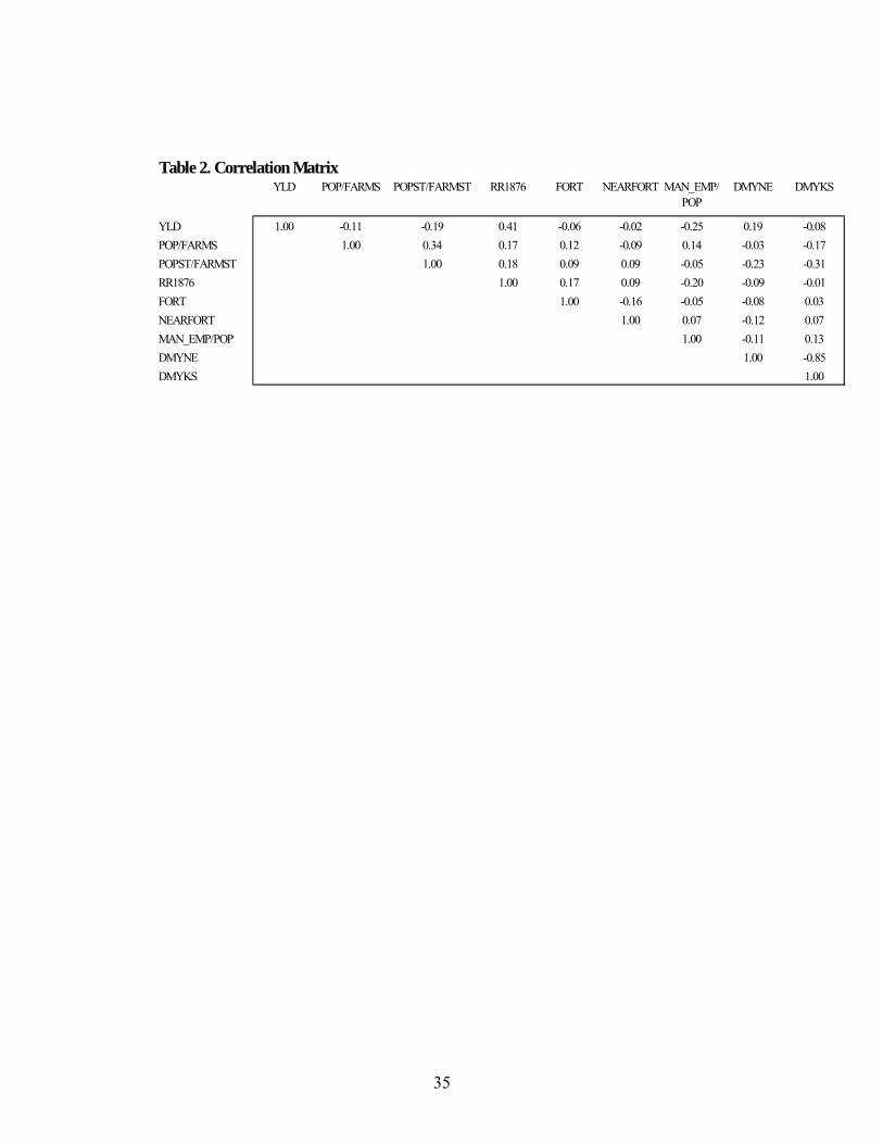
Finally, multicollinearity is a potential issue in any econometric exercise.

For example, it may be that forts were located in close proximity to rail lines,

suggesting a potentially high correlation between those two variables which could

bias these variables’ estimated standard errors upwards. Table 2 reports

correlation coefficients between the independent variables defined in equation (1).

Based on these statistics, there is little worry about statistical correlation between

variables, lessening the collinearity concern.16

15 Pendyck and Rubinfeld (1998) or Greene (1993) offers a good review of the TSLS procedure. In addition to the independent variables listed above, we include additional regressors necessary to identify the YLD equation in the initial stage of the TSLS procedure. In this equation, we include several regional variable indicators such as counties located east of the 98th meridian (for Kansas and Nebraska) and whether or not a county had a river passing through it. One would expect yields to be effected by lands east of the 98th meridian since rain fall is substantially higher in these locations relative the more arid conditions west of this delineation (see Webb, 1931). Moreover, if a county had a river passing through it might indicate easier access to water resource necessary for irrigation and cultivation. This too should directly impact yields. Finally, we include a variable: ACRES/FARMS, which measures the average size farm in a given county. To the extent that there are scale economies, one might expect productive yields to be higher on larger farms. These initial stage results, not presented here, are available upon request from the authors. It should be noted that an alternative approach to at least lessening the concern over endogeneity would be to obtain lagged YLD data from the 1870 census. Unfortunately, no such data is available. 16 That said, two observations are worth highlighting. First, the correlation between RR1876 and YLD is relatively high, perhaps suggesting that yields benefited from rail access making it easier to ship inputs into the area and product out. Since RR1876 is included in the initial stage modeling YLD in the TSLS procedure however, this correlation is less of an issue. Second, one may be concerned with potential endogeneity between the establishments of forts and population.

20

V. Results

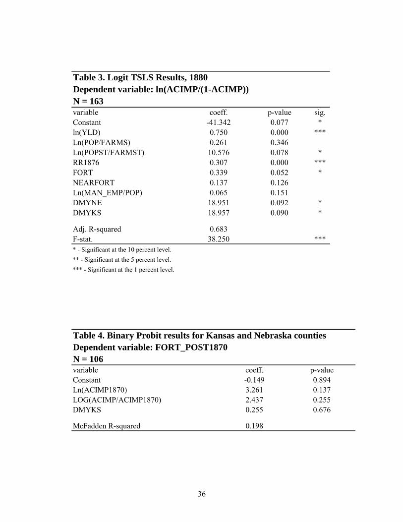
The TSLS results are presented in Table 3. The regression results appear

to be explaining about 68 percent of the dependent variable and the F-statistic

implied that we can comfortably reject the null hypothesis that our coefficients are

jointly equal to zero.

The key variable in our model is FORT, which proves to have a positive a

statistically significant determinant of ACIMP, suggesting that, after controlling

for other influences, greater capital investment and labor effort occurred in those

counties where a fort was present. In terms of magnitudes, the results indicate

that the presence of a nearby fort alone induces an increase in the proportion of

improved acres of about 1.24 percent on average, relative to those counties that

did not contain a fort.17 In light of previously published evidence by Craig,

Palmquist, and Weiss (1998) and Decker and Flynn (2007), indicating that land

values are significantly increased when land improvements occur, we conclude

that forts offer incentives to land improvement behavior, and therefore tend to

increase land values as well.

Specifically, one reason that the frontier army built forts in areas of greater settlement. While this is a possibility, there is little correlation between county population and the FORT variable. Second, Freedom’s (1987, p. 10) research states that in many cases fort construction generally preceded settlement in many frontier regions. 17 This effect was calculated in the following way. Since FORT is binary, we have for the Logit

model, FORT 1 FORT 0 0.3391y ACIMP ACIMP 0.584

e 1= = −Δ = − = =

+. To find the percent by which

ACIMP is impacted, we follow convention and evaluate this percentage at the mean value of our dependent variable. Specifically, we calculate: y / 47.1% 1.24Δ = .

21

The results also suggest closer proximity to a fort is more likely to induce

increased agricultural development, evidenced by the smaller coefficient on

NEARFORT. Also, at conventional significant levels, we cannot conclude that a

fort located adjacent to a particular county induces more agricultural activity,

although it is worth noting that the p-value is .126, “close” to the standard 10

percent significance level.

The other variables in the model generally come through as expected.

Land more conducive to agriculture, as proxied by YLD, tends to induce greater

land improvement activity. Indeed, a ten percent increase in YLD results in a

3.97 percent increase in ACIMP. 18 Moreover, those counties that have rail access

by 1880 also appear to experience greater agricultural land improvements.

While the coefficients are as expected on ln(POP/FARMS) and

ln(MAN_EMP/POP), neither is statistically significant at conventional levels.

Interestingly, larger state population relative to farms does not appear to prompt

more land improvements in counties, suggesting that by 1880 many farming

operations were inclined to look beyond local markets.

18 To calculate an elasticity for continuously defined variables, for the general logistic

model: ln ln1⎛ ⎞

=⎜ ⎟−⎝ ⎠

y xy

β , the resulting elasticity is (1 )yβ − . Again, following convention we

evaluate this elasticity at the mean of y. For the elasticity of YLD on ACIMP, we calculate 0.750*(1 0.470) 0.397− ≈ .

22

Is the location of a fort endogenous to land improvements? The issue of

how fort sites were determined is still open. One might suggest that forts were

located in areas where some farming/ranching activity had already taken place.

Such regions would be a potential source for food and other provisions required

by the stationed garrisons, although correlation statistics do not support this

assertion. That said, given that the underlying assumption in our model

necessarily assumes that forts impact land improvement and not vice versa, it is

worth addressing whether or not there is reason to suggest fort site selection

depended on land improvements. The issue of site selection is complex and we

do not presume to model the process completely, though we do offer some

evidence that dampens the concern over reverse causality. To address this issue

empirically, we collected data on the proportion of acreage improved to acres

from the Ninth Decennial Census of the United States of 1870, compiled by

ICPSR. We then created a binary variable, again using data from Hart (1963,

1964) that equals 1 when a military fort was constructed after 1870, 0 otherwise.

We then estimated the following model assuming a binary Probit19:

1

2 3

Pr( _ 1870 1) ( ln( 1870)ln( / 1870) ).

= = Φ ++ +

FORT POST ACIMPACIMP ACIMP DMYKSα β

β β

(2)

19 Note that we did lose data from Colorado as it was not a state in 1870 and we thus did not have county level data. This results in a reduced sample size to about 106 observations.

23

If fort site was sensitive to improved acreage, as well as any improved acreage

over the decade of the 1870s, we should expect positive and significant

coefficients on β1 and β2. The results are presented in Table 4. Neither variable

appears to be a determining factor of fort site location, calling into question

concerns that forts were selected in response to agricultural investment already

taken place.20

Did a fort sustain agricultural development? We began this essay by

discussing the relative value of governmental involvement in economic

development and, in particular, the Homestead Act of 1862. The suggestion was

that, while the act, and the several other land disposal acts that followed were

largely a failure because they fostered small scale farming on land not suited for

such operations, perhaps federal efforts to support farm success through

settlement protection, etc., may have played a role in fostering such development.

As the results above highlight, the establishment of military forts did foster land

development.

However, these results do not offer clues as to the impact that military

forts may have played in sustaining such agricultural efforts. This issue is

important since the failure of a military presence to translate into sustained

20 Note that the dummy variable for Kansas was included to capture any potential influence state political and other social differences may have played in fort location. Also note that the results are substantively the same either the level of acres improved in 1870 or the growth in acres improved is dropped from equation (2). Clearly, these results offer little insight as the cause of fort site selection. While beyond the scope of this study, such an analysis my be a fruitful avenue for future research.

24

growth, further calls into question 1) whether or not the establishment of forts

simply delayed the inevitable failure of the land acts and 2) whether or not the

establishment of forts caused too much agricultural investment to take place,

suggesting a socially inefficient commitment of agricultural capital investment

and labor effort.

In this section, we address the issue of whether or not a fort constructed

prior to 1880 but subsequently closed prior to 1890 resulted in sustained

agricultural growth in both land improvements and number of farms. This

hypothesis tests whether capital deepening in land improvement prompted by the

presence of a fort in 1880 was sufficient to sustain growth even after the military

(and the associated federal spending that supported the garrisons) exited the area.

If the answer is “yes”, such development was in fact sustained, then one would be

inclined to conclude that the frontier army did create circumstances that supported

development, perhaps mitigating the criticism of the Homestead Act of 1862. If,

however, the answer is “no” one might conclude the frontier army only delayed

the inevitable, that homesteading in certain regions was simply untenable.

We constructed two growth models to address this issue. The first models

the growth in ACIMP between 1880 and 1890. The second models the growth in

FARMS between 1880 and 1890. Data for 1890 on land improvements,

ACIMP1890, 1890 farms, FARMS1890, county and state (net of county i) level

population for 1890, POP1890 and POPST1890, and manufacturing employment

25

in 1890, MAN_EMP1890, were all taken from the Eleventh Decennial Census of

the United States of 1890, compiled by ICPSR. We constructed FORT_PRE1890,

again from Hart (1963, 1964), which indicates those forts which were in operation

in 1880 but subsequently closed prior to 1890. Indeed, most forts in our dataset

were indeed closed by 1890. We also created a variable, RR_ADDED, which is a

dummy variable indicating if a county that did not have a rail line in 1876 did

receive such a line by the 1890s.21

We estimated the following equation via TSLS:

i i 1 i 2 i i

3 i i

4 i i

5 i 6 i

7 8 i

ln(X1890 / X ) ln(YLD ) ln(POP1890 / POP )ln(POPST1890 / POPST )ln(MAN _ EMP1890 / MAN _ EMP )RR _ ADDED FORT _ PRE1890DMYKS DMYNE e

= αβ +β+β+β+β +β+β +β +

,

(3)

where Xi equals either ACIMP or FARMS for a given county i.22 We would

expect a positive coefficient on the two population growth variables as well as the

manufacturing employment growth variable. We also would expect continued

21 Annual data on rail construction by county is not available. To get a picture of the progression of rail construction through the period of interest we exploited data from the following web site http://www.livgenmi.com/1895/, which supplies data on the location of rail lines by state and county for the year 1895. While there may be some concern that we have counted counties that may have had rails by 1895 but not as of 1890, it is generally accepted that most of the major rail lines were build by the 1890s. Hence, while available data does not exist to verify with certainty, any bias in our data is likely small. 22 Note that we still estimate our equation (3) using TSLS owning to the endogeneity of YLD being driven by locational and land attribute factors (such as the presence of a river in the county). We also account for potential heteroscedasticity using White’s estimator. The results are not substantively different from OLS.

26

growth due to the spreading of the railroad network. We would expect a negative

coefficient on YLD (i.e. productive yields as of 1880 as a proxy for land quality)

under the hypothesis that, as a measure of land quality, the most productive acres

of land would be used for production first. Also, we control for potential

differences across states. Finally, if the military was to sustain growth after fort

abandonment, we would expect the coefficient of FORT_PRE1890 to be positive

as well.

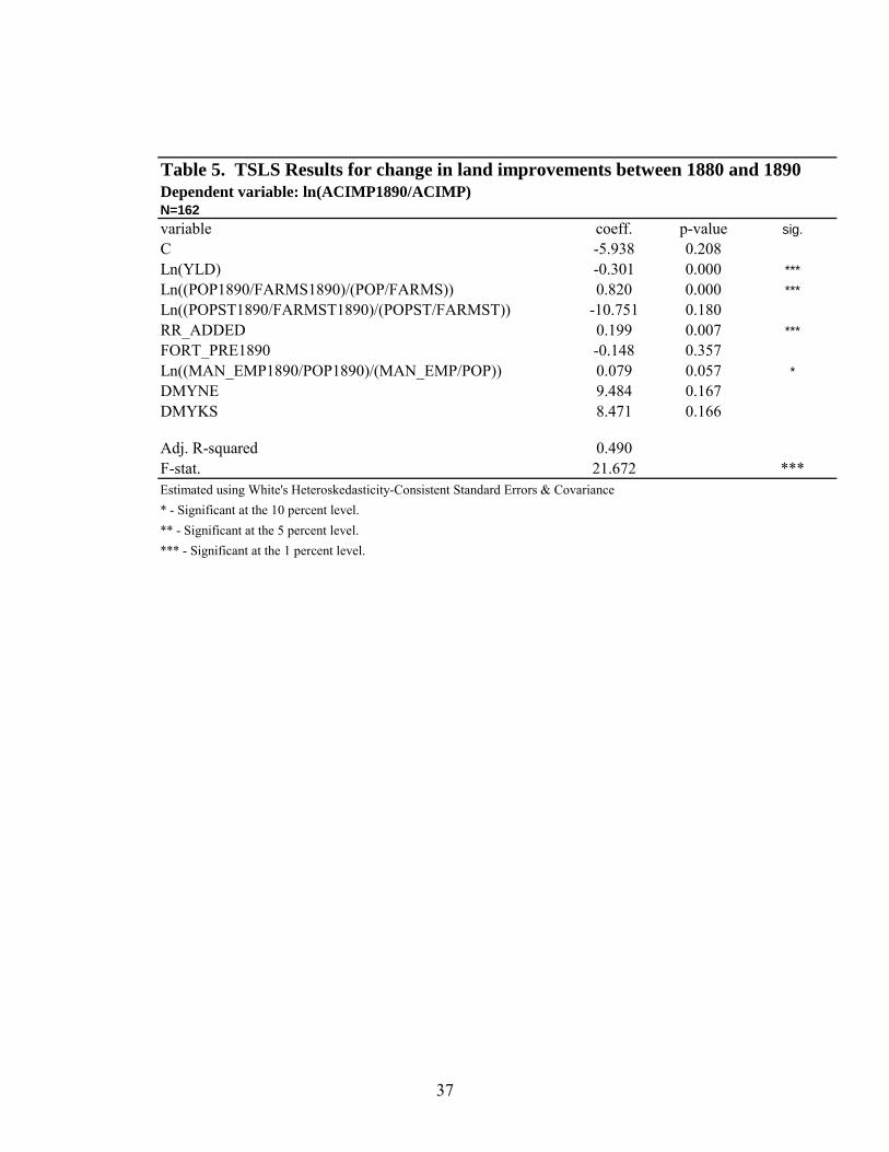
The results for the land improvement growth equation are presented in

Table 5. We find that local population growth, local manufacturing growth, and

the acquisition of a rail line increased growth in land development. We find, as

expected, that higher productive yields in 1880, ceteris paribus, tend to slow land

development. Finally, we find that the initial presence of a military fort has no

statistical impact on the growth of land development.

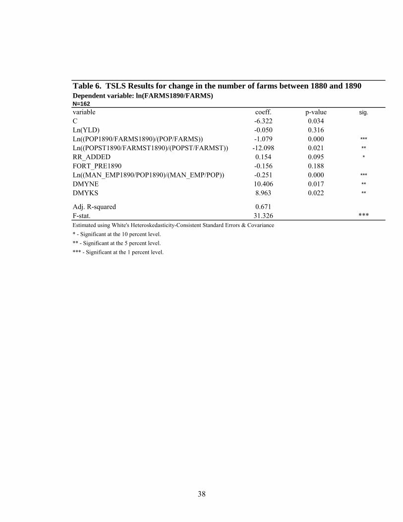
Turning attention to the growth in the number of farms, Table 6, we find

that farm growth was deterred by increases in population and manufacturing,

contrary to the results presented in Table 5. This is likely due to a crowding out

effect; the more population and manufacturing, the less land available for new

farms. We also find, consistent with Table 5, that gaining rail access, ceteris

paribus, did foster some farm growth. However, we find that the initial presence

of a fort did not support continued farm development. Indeed, since our measure

of farm growth is in fact net farm growth, some of the farms from 1880 failed by

27

1890, thus slowing the overall growth in farms over the period. Apparently, even

the presence of a military establishment could not salvage the nation’s land

disposal policies.23

VI. Conclusion

In this paper we empirically investigated the relationship between

agricultural development in Kansas, Nebraska, and Colorado and proximity to

military forts in 1880. We find that, ceteris paribus, agricultural investments are

substantially higher in those counties where a military fort is present, suggesting

that military forts had a stimulating impact on agricultural development in the

Great Plains. However, the reverse is not true. There is no statistical support for

the notion that forts necessarily located in counties where substantial investment

already occurred. Moreover, we found that while the presence of a military fort

has the effect of increasing agricultural development, there is no evidence that

such a presence sustained agricultural development.

While federal expenditures on military support appear to have had an

immediate impact on agricultural investments in land, capital and labor, it was not

sustained. As a result, it is entirely possible that the presence of a fort prompted

more investment that would otherwise have been warranted, suggesting that in the

23 In and ideal world, it would be of value to look specifically at farm failure (and new farm additions). Indeed, it would be of interest to consider more directly the impact of military forts and farm failures. In light of the evidence presented here, it is likely that the presence of a nearby fort would not have delayed farm failures by much, if at all. Nonetheless, it would be useful to investigate this. However, such data is not available from the Census. We leave this for future research.

28

end, not only could farm establishment growth not be sustained, more resources

were devoted to such development that would be socially optimal.

There are several avenues of future research. For instance, a richer

exploration of the determinants of fort locations would be an interesting exercise.

Moreover, a breakdown of the determinants of farm failures and new farm

formation specifically would offer some additional insights to the results

presented in our Table 6. Finally, it would be of interest to compare these results

to fort locations in and the development of mining operations in the nineteenth

century and compare with the results we have found here for agricultural

development. These we leave for future research.

29

Bibliography

Anderson Terry L. and Peter J. Hill, “Evolution of Property Rights: A Study of the American West,” Journal of Law & Economics 18(1), 1975, pp. 163-179.

-----------, “Race for Property Rights,” Journal of Law & Economics 33(1), 1990,

99. 177-197. -----------, The Not So Wild, Wild West: Property Rights on the Frontier. Stanford,

CA: Stanford University Press. 2004. Anderson, Terry L. and Donald R. Leal. Free Market Environmentalism.

Boulder: Westview Press, Inc. 1991. Becsi, Zsolt. Do State and Local Taxes Affect Relative State Growth?” Economic

Review, March/April. 1996: pp. 18-36. Besley, Timothy. “Property Rights and Investment Incentives: Theory and

Evidence from Ghana,” Journal of Political Economy 1995, 103(5): pp. 903-937.

Chandra, Amitabh, and Thompson, Eric. “Does Public Infrastructure Affect

Economic Activity? Evidence from the Rural Interstate Highway System? Evidence From the Rural Interstate Highway System,” Regional Science and Urban Economics. 30 (4) 2000: pp. 457-90.

Craft, Eric, D. “The Value of Weather Information Services for Nineteenth

Century Great Lakes Shipping, American Economic Review. 1998. 88(5): pp. 1059-1076.

Craig, L., and R. Palmquist, and T. Weiss, “Transportation Improvements and

Land Values in the Antebellum United States: A Hedonic Approach,” Journal of Real Estate Finance and Economics 16(2), 1998, pp. 173-189.

Cunfer, Geoff. On the Great Plains: Agriculture and Environment. College

Station: Texas A&M University Press, 2005. Decker, Christopher S., and Flynn, David T. “The Railroad’s Impact on Land

Values in the Upper Great Plains at the Closing of the Frontier,” Historical Methods 40(1), 2007, pp. 28-38.

30

Dobak, William A. Fort Riley and its Neighbors: Military Money and Economic

Growth, 1853-1895. Norman, OK: University of Oklahoma Press. 1998. Dunn Jr., Walter S. Opening New Markets: The British Army and the Old

Northwest, Westport, CT. Praeger. 2002. Frazer, Robert W. Forts of the West: Military Forts and Presidios and Posts

Commonly Called Forts West of the Mississippi River to 1898, 7th ed. Norman, OK: University of Oklahoma Press. 1988.

Freedom, Gary S. “The Role of the Military and the Spread of Settlement in the

Northern Great Plains, 1866-1891,” The Midwest Review 9, 1987: pp. 1-11.

Greene, William H., Econometric Analysis, Englewood Cliffs: Prentice-Hall,

1993. Hansen, Zeynep Kocabiyik and Libecap, Gary D. “The Allocation of Property

Rights to Land: US Land Policy and Farm Failure in the Northern Great Plains,” Explorations in Economic History 2004, 42(2): 103-129.

Hart, Herbert, M. Old Forts of the Northwest. Seattle, WA: Superior Publishing

Press. 1963. ----------------. Old Forts of the Southwest. Seattle, WA: Superior Publishing

Press. 1964. Hine, Robert V., and Faragher, John Mack. The American West: A New

Interpretive History. New Haven, CT: Yale University Press, 2000 Hooker, Mark A. and Knetter, Michael M. “Measuring the Economic Effects of

Military Base Closures,” Economic Inquiry. 39(4), 2001: pp. 583-598. Kmenta, Jan. 1986. Elements of Econometrics, 2nd ed. New York: Macmillan. Kanazawa, Mark. “Investment in Private Water Development: Property Rights

and Contractual Opportunism During the California Gold Rush,” Explorations in Economic History 2006, 43: pp. 357-381.

31

Libecap, Gary D. and Hansen, Zeynep Kocabiyik. “’Rain Follows the Plow’ and Dryfarming Doctrine: The Climate Information Problem and Homestead Failure in the Upper Great Plains, 1890-1925,” The Journal of Economic History 2002, 62(1): pp. 86-120.

Lindert, Peter. “Long Run Trends in American Farmland Values.” In

Quantitative Studies in Agrarian History, ed. Morton Rothstein and Daniel Field. Ames: Iowa State University Press, 1993.

Malone, Laurence J. Opening the West: Federal Internal Improvements Before

1860. Westport, CT: Greenwood Press. 1998. North, Douglass C. “Institutions, Transactions Costs and Economic Growth,”

Economic Inquiry 1987, 25(3): pp. 419-428. ---------------. Institutions, Institutional Change and Economic Performance,

Cambridge, MA. Cambridge University Press. Olson, James C. and Naugle, Ronald C. History of Nebraska, 3rd ed. Lincoln, NE:

University of Nebraska Press. 1997. Pindyck, Robert S., and Rubinfeld, Daniel L. Econometric Models and Economic

Forecast, 4th ed. Boston, MA: Irwin McGraw-Hill. 1998. Rand McNally’s Pioneer Atlas of the American West. Chicago: Rand McNally &

Company, 1969. Stewart, James I. “Migration to the Agricultural Frontier and Wealth

Accumulation, 1860-1870,” Explorations in Economic History. 2005, forthcoming.

Tate, Michael L. The Frontier Army in the Settlement of the West. Norman, OK:

University of Oklahoma Press. 1999. Tate, Michael L. The American Army in Transition, 1865-1898. Westport, CT:

Greenwood Press. 2007. Torstensson, Johan. “Property Rights and Economic Growth: An Empirical

Study,” Kyklos 1994, 47(2): pp. 231-247.

32

U.S. Bureau of the Census. 1883-1888. Statistics of Population 1883, Volume I: Table 23.

U.S. Bureau of the Census. 1883. Report on the Production of Agriculture 1883,

Volume III: Table 7. Walton, Gary M., and Rockoff, Hugh. History of The American Economy, 8th ed.

New York: Dryden Press, 1998. Webb, Walter P. The Great Plains. Lincoln: University of Nebraska Press, 1931. White, Richard. It’s Your Misfortune and None of My Own: A New History of the

American West. Norman: University of Oklahoma Press, 1991.

33

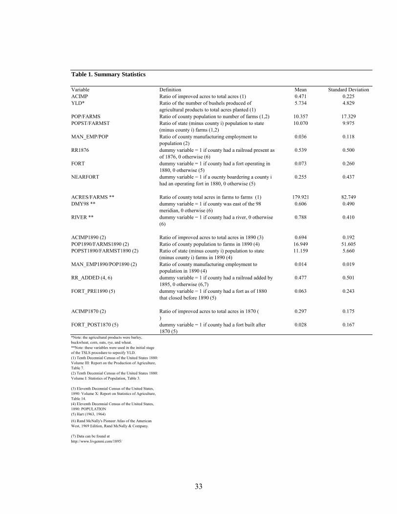
Table 1. Summary Statistics

Variable Definition Mean Standard DeviationACIMP Ratio of improved acres to total acres (1) 0.471 0.225YLD* Ratio of the number of bushels produced of

agricultural products to total acres planted (1)5.734 4.829

POP/FARMS Ratio of county population to number of farms (1,2) 10.357 17.329POPST/FARMST Ratio of state (minus county i) population to state

(minus county i) farms (1,2)10.070 9.975

MAN_EMP/POP Ratio of county manufacturing employment to population (2)

0.036 0.118

RR1876 dummy variable = 1 if county had a railroad present as of 1876, 0 otherwise (6)

0.539 0.500

FORT dummy variable = 1 if county had a fort operating in 1880, 0 otherwise (5)

0.073 0.260

NEARFORT dummy variable = 1 if a oucnty boardering a county i had an operating fort in 1880, 0 otherwise (5)

0.255 0.437

ACRES/FARMS ** Ratio of county total acres in farms to farms (1) 179.921 82.749DMY98 ** dummy variable = 1 if county was east of the 98

meridian, 0 otherwise (6)0.606 0.490

RIVER ** dummy variable = 1 if county had a river, 0 otherwise (6)

0.788 0.410

ACIMP1890 (2) Ratio of improved acres to total acres in 1890 (3) 0.694 0.192POP1890/FARMS1890 (2) Ratio of county population to farms in 1890 (4) 16.949 51.605POPST1890/FARMST1890 (2) Ratio of state (minus county i) population to state

(minus county i) farms in 1890 (4)11.159 5.660

MAN_EMP1890/POP1890 (2) Ratio of county manufacturing employment to population in 1890 (4)

0.014 0.019

RR_ADDED (4, 6) dummy variable = 1 if county had a railroad added by 1895, 0 otherwise (6,7)

0.477 0.501

FORT_PRE1890 (5) dummy variable = 1 if county had a fort as of 1880 that closed before 1890 (5)

0.063 0.243

ACIMP1870 (2) Ratio of improved acres to total acres in 1870 ( )

0.297 0.175

FORT_POST1870 (5) dummy variable = 1 if county had a fort built after 1870 (5)

0.028 0.167

*Note: the agricultural products were barley, buckwheat, corn, oats, rye, and wheat.**Note: these variables were used in the initial stage of the TSLS procedure to sepecify YLD.(1) Tenth Decennial Census of the United States 1880: Volume III: Report on the Production of Agriculture, Table 7.(2) Tenth Decennial Census of the United States 1880: Volume I: Statistics of Population, Table 3.

(3) Eleventh Decennial Census of the United States, 1890: Volume X: Report on Statistics of Agriculture, Table 14.(4) Eleventh Decennial Census of the United States, 1890: POPULATION(5) Hart (1963, 1964)

(6) Rand McNally's Pioneer Atlas of the American West, 1969 Edition, Rand McNally & Company.

(7) Data can be found at http://www.livgenmi.com/1895/

34

35

Table 2. Correlation MatrixYLD POP/FARMS POPST/FARMST RR1876 FORT NEARFORT MAN_EMP/

POPDMYNE DMYKS

YLD 1.00 -0.11 -0.19 0.41 -0.06 -0.02 -0.25 0.19 -0.08POP/FARMS 1.00 0.34 0.17 0.12 -0.09 0.14 -0.03 -0.17POPST/FARMST 1.00 0.18 0.09 0.09 -0.05 -0.23 -0.31RR1876 1.00 0.17 0.09 -0.20 -0.09 -0.01FORT 1.00 -0.16 -0.05 -0.08 0.03NEARFORT 1.00 0.07 -0.12 0.07MAN_EMP/POP 1.00 -0.11 0.13DMYNE 1.00 -0.85DMYKS 1.00

36

Table 3. Logit TSLS Results, 1880Dependent variable: ln(ACIMP/(1-ACIMP))N = 163 variable coeff. p-value sig.Constant -41.342 0.077 *ln(YLD) 0.750 0.000 ***Ln(POP/FARMS) 0.261 0.346Ln(POPST/FARMST) 10.576 0.078 *RR1876 0.307 0.000 ***FORT 0.339 0.052 *NEARFORT 0.137 0.126Ln(MAN_EMP/POP) 0.065 0.151DMYNE 18.951 0.092 *DMYKS 18.957 0.090 *

Adj. R-squared 0.683F-stat. 38.250 **** - Significant at the 10 percent level.** - Significant at the 5 percent level.*** - Significant at the 1 percent level. Table 4. Binary Probit results for Kansas and Nebraska counties Dependent variable: FORT_POST1870N = 106variable coeff. p-valueConstant -0.149 0.894Ln(ACIMP1870) 3.261 0.137LOG(ACIMP/ACIMP1870) 2.437 0.255DMYKS 0.255 0.676

McFadden R-squared 0.198

37

Table 5. TSLS Results for change in land improvements between 1880 and 1890Dependent variable: ln(ACIMP1890/ACIMP)N=162variable coeff. p-value sig.C -5.938 0.208Ln(YLD) -0.301 0.000 ***Ln((POP1890/FARMS1890)/(POP/FARMS)) 0.820 0.000 ***Ln((POPST1890/FARMST1890)/(POPST/FARMST)) -10.751 0.180RR_ADDED 0.199 0.007 ***FORT_PRE1890 -0.148 0.357Ln((MAN_EMP1890/POP1890)/(MAN_EMP/POP)) 0.079 0.057 *DMYNE 9.484 0.167DMYKS 8.471 0.166

Adj. R-squared 0.490F-stat. 21.672 ***Estimated using White's Heteroskedasticity-Consistent Standard Errors & Covariance* - Significant at the 10 percent level.** - Significant at the 5 percent level.*** - Significant at the 1 percent level.

38

Table 6. TSLS Results for change in the number of farms between 1880 and 1890Dependent variable: ln(FARMS1890/FARMS)N=162variable coeff. p-value sig.C -6.322 0.034Ln(YLD) -0.050 0.316 Ln((POP1890/FARMS1890)/(POP/FARMS)) -1.079 0.000 ***Ln((POPST1890/FARMST1890)/(POPST/FARMST)) -12.098 0.021 **RR_ADDED 0.154 0.095 *FORT_PRE1890 -0.156 0.188Ln((MAN_EMP1890/POP1890)/(MAN_EMP/POP)) -0.251 0.000 ***DMYNE 10.406 0.017 **DMYKS 8.963 0.022 **

Adj. R-squared 0.671F-stat. 31.326 ***Estimated using White's Heteroskedasticity-Consistent Standard Errors & Covariance* - Significant at the 10 percent level.** - Significant at the 5 percent level.*** - Significant at the 1 percent level.