The geometry of impossible gures - ATCM

The geometry of impossible figures

Alasdair McAndrew Jacob A. C. [email protected] [email protected]

College of Engineering and Science Mathematics DepartmentVictoria University Alexandra Park School

PO Box 14428, Melbourne 8001 Bidwell Gardens, London N11 2AZAustralia United Kingdom

Abstract

“Impossible figures” are those that can be drawn with perspective in two dimensions,but cannot exist in the physical world. Well known examples are the Penrose triangle, thePenrose staircase, and the “impossible trident”. The Dutch artist Maurits Escher (1898–1972) took great delight in such figures and incorporated them into many of his works.Less well known is the Swedish artist and graphics designer Oscar Reutersvard (1916–2002), who drew and developed hundreds of such figures, and who has been honoured bysome Swedish postage stamps showing his designs. Some art installations now includesuch figures, but which only seem impossible from one particular perspective. In thisarticle, we explore the geometry of such figures, and discuss how such figures can bedrawn using standard programming tools. The mathematics required is elementary, butnot without subtlety, and with the delight of producing some lovely diagrams.

1 The big three

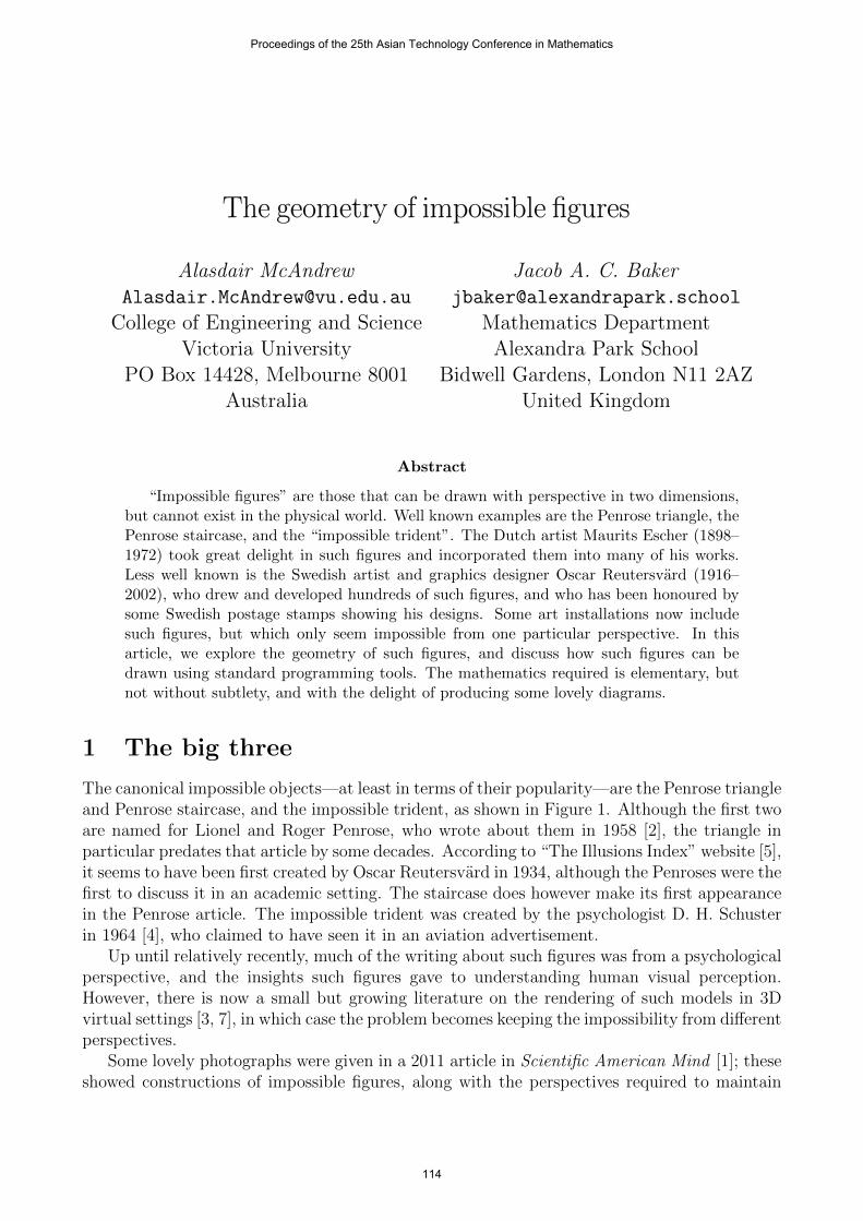
The canonical impossible objects—at least in terms of their popularity—are the Penrose triangleand Penrose staircase, and the impossible trident, as shown in Figure 1. Although the first twoare named for Lionel and Roger Penrose, who wrote about them in 1958 [2], the triangle inparticular predates that article by some decades. According to “The Illusions Index” website [5],it seems to have been first created by Oscar Reutersvard in 1934, although the Penroses were thefirst to discuss it in an academic setting. The staircase does however make its first appearancein the Penrose article. The impossible trident was created by the psychologist D. H. Schusterin 1964 [4], who claimed to have seen it in an aviation advertisement.

Up until relatively recently, much of the writing about such figures was from a psychologicalperspective, and the insights such figures gave to understanding human visual perception.However, there is now a small but growing literature on the rendering of such models in 3Dvirtual settings [3, 7], in which case the problem becomes keeping the impossibility from differentperspectives.

Some lovely photographs were given in a 2011 article in Scientific American Mind [1]; theseshowed constructions of impossible figures, along with the perspectives required to maintain

Proceedings of the 25th Asian Technology Conference in Mathematics

114

[email protected]

[email protected]

the illusion of impossibility, as well as shots from other perspectives which ruined the illusionbut demonstrated the constructions.

However, as far as we can determine, there is very little material about the two dimensionalgeometry of these figures—given that as “impossible figures” they can only truly be said to existin the plane. A partial discussion was begun by Uribe [6] who also gave a simple algorithm todetermine if a figure such as the Penrose triangle was in fact impossible. (Fundamentally thisconsisted of crawling round the figure taking into account corners as projections from three-dimensional Euclidean space and noting the change in direction at each corner, and checking ifsuch a crawl returned to the starting coordinates.) We shall explore several different approachesto their geometry, with the outcome of being able to draw them using any computer softwarethat can draw lines and polygons. We shall be using Python because we both know it, it’s free,and there are versions for all platforms. Given that Python code is mostly self explanatory,our code should be easily transferable to other systems. Note that all the code in this paper isavailable online at https://bit.ly/baker_mcandrew, and can be run at that site, so everythingin this paper can be explored without having to download Python or any of its libraries ormodules.

Penrose triangle Penrose staircase Impossible trident

Figure 1: Three impossible figures

2 The Penrose triangle

In many ways this is the most satisfying of all to draw by hand; if you can draw an equilateraltriangle and a straight line, then you can draw this figure. Figure 2 shows its evolution in asequence of straight lines starting from an equilateral triangle.

Figure 2: Drawing a Penrose triangle


115

https://bit.ly/baker_mcandrew

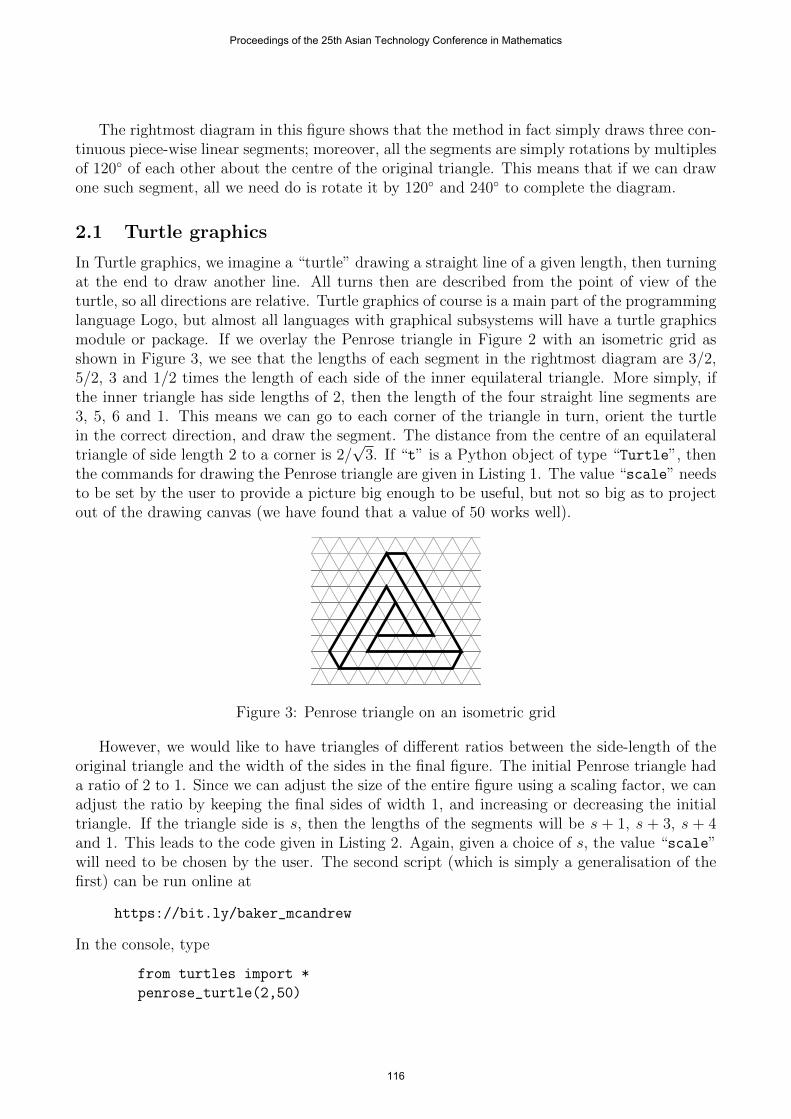
The rightmost diagram in this figure shows that the method in fact simply draws three con-tinuous piece-wise linear segments; moreover, all the segments are simply rotations by multiplesof 120◦ of each other about the centre of the original triangle. This means that if we can drawone such segment, all we need do is rotate it by 120◦ and 240◦ to complete the diagram.

2.1 Turtle graphics

In Turtle graphics, we imagine a “turtle” drawing a straight line of a given length, then turningat the end to draw another line. All turns then are described from the point of view of theturtle, so all directions are relative. Turtle graphics of course is a main part of the programminglanguage Logo, but almost all languages with graphical subsystems will have a turtle graphicsmodule or package. If we overlay the Penrose triangle in Figure 2 with an isometric grid asshown in Figure 3, we see that the lengths of each segment in the rightmost diagram are 3/2,5/2, 3 and 1/2 times the length of each side of the inner equilateral triangle. More simply, ifthe inner triangle has side lengths of 2, then the length of the four straight line segments are3, 5, 6 and 1. This means we can go to each corner of the triangle in turn, orient the turtlein the correct direction, and draw the segment. The distance from the centre of an equilateraltriangle of side length 2 to a corner is 2/

√3. If “t” is a Python object of type “Turtle”, then

the commands for drawing the Penrose triangle are given in Listing 1. The value “scale” needsto be set by the user to provide a picture big enough to be useful, but not so big as to projectout of the drawing canvas (we have found that a value of 50 works well).

Figure 3: Penrose triangle on an isometric grid

However, we would like to have triangles of different ratios between the side-length of theoriginal triangle and the width of the sides in the final figure. The initial Penrose triangle hada ratio of 2 to 1. Since we can adjust the size of the entire figure using a scaling factor, we canadjust the ratio by keeping the final sides of width 1, and increasing or decreasing the initialtriangle. If the triangle side is s, then the lengths of the segments will be s + 1, s + 3, s + 4and 1. This leads to the code given in Listing 2. Again, given a choice of s, the value “scale”will need to be chosen by the user. The second script (which is simply a generalisation of thefirst) can be run online at


In the console, type

from turtles import *

penrose_turtle(2,50)


116


to see it.

Listing 1: Turtle graphics

import turtle as t

from math import sqrt

scale = 50

for angle in [0,120,240]:

t.penup()

t.goto(0,0)

t.setheading(angle)

t.forward(2*scale/sqrt(3))

t.left(150)

t.pendown()

t.forward(3*scale)

t.left(120)

t.forward(5*scale)

t.left(120)

t.forward(6*scale)

t.left(60)

t.forward(1*scale)

Listing 2: Turtle graphics with scale

s = 2

for angle in [0,120,240]:

t.penup()

t.goto(0,0)

t.setheading(angle)

t.fd(s*scale/sqrt(3))

t.left(150)

t.pendown()

t.forward((s+1)*scale)

t.left(120)


t.left(120)


t.left(60)

t.forward(scale)

2.2 Cartesian coordinates

Consider the segment starting at the bottom left corner of the original triangle: the segmentshown with the continuous line. Again using an initial side length of 2, we find by chasingcoordinates and angles that the end points of the straight line segments are:

(−1,−1/√

3), (2,−1/√

3), (−1/2, 13/√

12), (−7/2,−5/√

12), (−3,−4/√

3).

This can be written in Python using the “numpy” library as an array (a matrix) in which thetop row contains all the x coordinates, and the bottom row the y coordinates. Now all we needdo is rotate these points, which can be done using the standard rotation matrix With thesedefinitions and imports, the remainder of the script is straight forward and is given in Listing 3.This code can be run at https://bit.ly/baker_mcandrew as before; choose the main.py file,run it, and then use penrose1() to display it.

Listing 3: Cartesian definition of the Penrose triangle

import matplotlib.pyplot as plt

from numpy import array, sqrt, sin, cos, pi

# Enter the matrix of vertices of one path

pts = array([[-1,2,-1/2,-7/2,-3],\

[-1/sqrt(3),-1/sqrt(3),13/sqrt(12),-5/sqrt(12),-4/sqrt(3)]])

# Define the rotation matrix and the other two paths

rotate = lambda x: array([[cos(x),-sin(x)],[sin(x),cos(x)]])

pts_2 = rotate(2*pi/3).dot(pts)

pts_3 = rotate(4*pi/3).dot(pts)


117


# Now plot each path

fig, ax = plt.subplots(figsize=(6,6))

ax.plot(pts[0],pts[1],’k-’)

ax.plot(pts_2[0],pts_2[1],’k-’)

ax.plot(pts_3[0],pts_3[1],’k-’)

ax.set_aspect(’equal’)

plt.show()

2.3 Affine transformation

An affine transformation is a transformation that may includes a linear transformation of thecoordinates, and also a shift. Linear transformations can be done by matrix multiplication;shifting can also be so done, but needs to work with homogeneous coordinates (x : y : z) (withz 6= 0), where such a triple corresponds to the point (x/z, y/z) in the Cartesian plane. Anaffine transformation matrix will have the forma b e

c d f0 0 1

where the top left 2× 2 submatrix provides the linear transformation, and the top right 2× 1submatrix the shift. In our case we only need a linear transformation, and so the values e andf will be zero.

To see how this may simplify the description of the Penrose triangle, consider an isometricgrid, and with a y axis at 60 degrees to the x axis. The left hand diagram in Figure 4 showsthis grid with the first segment on it. To simplify the working, we will use an initial trianglewith side length of 3; this will ensure that all corners of segments will have integer coordinates.

x

y

x

y

Figure 4: Two different approaches to transformations

On these axes, the coordinates that define the segment are

(−1,−1), (3,−1), (−3, 5), (−3,−2), (−2,−3).

and the matrices corresponding to rotations by 120 and 240 degrees are[−1 −1

1 0

]and

[0 1−1 −1

]


118

respectively.In Python all this can be neatly generated with the code in Listing 4. The slightly mysteri-

ous “transform=A+ax.trandData” in the penultimate line simply applies the affine transformdefined by the matrix A to the points. This requires that the points themselves can first be givenas a “transform” type to which other transforms can be applied; thus the term “ax.transData”.This code is available at the same site as previously, by running penrose2().

Listing 4: Plotting the Penrose triangle using an affine transformation

import numpy as np

import matplotlib.pyplot as plt

from math import sqrt

from matplotlib.transforms import Affine2D

A = Affine2D(np.array([[1,1/2,0],[0,sqrt(3)/2,0],[0,0,1]]))

figure, ax = plt.subplots(figsize=(6,6))

R = np.array([[-1,-1],[1,0]])

pts1 = [[-1,3,-3,-3,-2],[-1,-1,5,-2,-3]]

pts2 = R.dot(pts1)

pts3 = R.dot(pts2)

for p in [pts1,pts2,pts3]:

ax.plot(p[0],p[1],’k-’,transform=A+ax.transData)

ax.set_aspect(’equal’)

plt.show()

Alternatively, we can plot the triangle directly onto a standard Cartesian plain as shownon the right in Figure 4, and simply rescale the axes so that they have the ratio 1 :

√3, which

means stretching the y axis by a factor of√

3 . This is trivial in Python as shown in Listing 5.

Listing 5: Using scaled axes to plot the Penrose triangle

figure,ax = plt.subplots()

ax.plot([-2,4,-1,-7,-6],[-1,-1,4,-2,-3],’k-’)

ax.plot([2,-1,-6,6,7],[-1,2,-3,-3,-2],’k-’)

ax.plot([0,-3,7,1,-1],[1,-2,-2,4,4],’k-’)

ax.set_aspect(sqrt(3))

Unfortunately this method, while conceptually very simple, does not allow the transforma-tion of one path to another by an affine transformation. This can be seen by considering apossible transformation defined by a matrix product and a shift. In terms of the matrices, thenwe would want:[

a bc d

] [−2 4 −1 −7 −6−1 −1 4 −2 −3

]+

[e e e e ef f f f f

]=

[2 −1 −6 6 7−1 2 −3 −3 −2

]where the two numeric matrices are the coordinates of two of the paths, and the symbolicmatrices represent the linear transformation and the shift. The left hand side can be expressedas a single 2× 5 matrix

M =

[−2a− b + e 4a− b + e −a + 4b + e −7a− 2b + e −6a− 3b + e−2c− d− f 4c− d− f −c + 4d− f −7c− 2d− f −6c− 3d− f

]


119

and equating each element with the corresponding element in the right hand matrix will producea linear system

AX = B

where X consists of the variables a, b, c, d, e, f , the elements of A are the coefficients of eachvariable from M , and B is simply the elements from the right.

A standard computation will determine that

rank(A) = 6, rank(A|B) = 7

and hence the equations are not solvable.

3 The Reutersvard triangle

This triangle seems to predate the Penrose triangle by many years. Instead of showing a trianglepurportedly of continuous beams, the triangle is constructed of a sequence of separated cubes.The result is quite striking, but unlike the Penrose triangle it is harder to draw by hand.However, as we shall see, it is not hard to program.

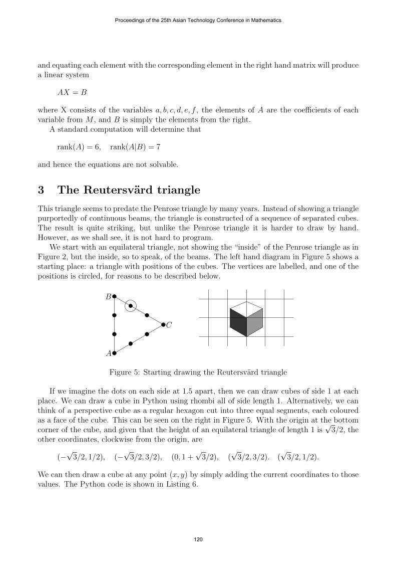
We start with an equilateral triangle, not showing the “inside” of the Penrose triangle as inFigure 2, but the inside, so to speak, of the beams. The left hand diagram in Figure 5 shows astarting place: a triangle with positions of the cubes. The vertices are labelled, and one of thepositions is circled, for reasons to be described below.

A

B

C

Figure 5: Starting drawing the Reutersvard triangle

If we imagine the dots on each side at 1.5 apart, then we can draw cubes of side 1 at eachplace. We can draw a cube in Python using rhombi all of side length 1. Alternatively, we canthink of a perspective cube as a regular hexagon cut into three equal segments, each colouredas a face of the cube. This can be seen on the right in Figure 5. With the origin at the bottomcorner of the cube, and given that the height of an equilateral triangle of length 1 is

√3/2, the

other coordinates, clockwise from the origin, are

(−√

3/2, 1/2), (−√

3/2, 3/2), (0, 1 +√

3/2), (√

3/2, 3/2). (√

3/2, 1/2).

We can then draw a cube at any point (x, y) by simply adding the current coordinates to thosevalues. The Python code is shown in Listing 6.


120

Listing 6: Code for drawing a cube

def cube(c):

x,y = c

s = sqrt(3)/2

right = [[x,y],[x+s,y+1/2],[x+s,y+3/2],[x,y+1],[x,y]]

left = [[x,y],[x-s,y+1/2],[x-s,y+3/2],[x,y+1],[x,y]]

top = [[x,y+1],[x+s,y+3/2],[x,y+2],[x-s,y+3/2],[x,y+1]]

return([right,left,top])

Given the orientation of the cube, in order to provide a three dimensional perspective, with“front” cubes blocking out “back” cubes, we start with the circled circle in Figure 5, and workclockwise from there. The simplest way to do this is to write all the points in a list, and drawa cube at each point. Each cube will be drawn on top of any previously drawn cubes, so thatthere’s no need for hidden line algorithms. The list is:

(3√

3/4, 15/4), (3√

3/2, 3), (9√

3/4, 9/4), (3√

3/2, 3/2), (3√

3/4, 3/4),

(0, 0), (0, 3/2), (0, 3), (0, 9/2).

We see this by assuming that the dots on each side of the triangle are spaced by 3/2. Thismeans that as we move left to right along either the top or bottom edge, the y value changesby 3/4, and the x value by 3/2 ×

√3/2 = 3

√3/4. However, before we start to put this into a

program, we can also generalise it, by the number of cubes per side, and the relative distancebetween each cube. This last can be expressed as a fraction of the cube’s side, so that in thecurrent example this distance is 0.5.

Suppose that we have n cubes per side, and a distance apart of d. Then with the trianglein the same orientation as in Figure 5, the left hand vertical side will have length (n−1)(d+ 1)since we assume that the cubes have length 1, and so there are n− 1 spaces between the firstand last positions of the cubes, and the distance of each will be d+ 1. The rightmost vertex Cof the triangle will then have the coordinates

x = (n− 1)(d + 1)

√3

2, y =

1

2(n− 1)(d + 1).

For sides AC and BC, the distance between consecutive x and y positions will be

∆x = (d + 1)

√3

2, ∆y =

d + 1

2.

The top side AC of the triangle will then consist of the positions(k∆x, (n− 1)(d + 1)− k∆y

), k = 0, 1, 2, . . . n− 1.

The bottom side BC positions are very similar:

(k∆x, k∆y) , k = 0, 1, 2, . . . n− 1.

Now it’s matter of putting all of this into a program. To draw the cubes in Python, we willuse the Polygon command from the patch library, which allows the easy drawing of polygons,and which are drawn over by subsequent polygons.


121

The result of this is shown on the left in Figure 6. However, there’s nothing particularly“impossible” about this figure: it just shows a sequence of cubes in space. The impossibilitycomes from re-drawing the second-top cube of the top edge of the triangle so that it seems tocome in front. This is done simply by re-drawing its left and top sides. This extra code is addedbefore the setting of the x and y limits above. The result is shown on the right in Figure 6,and this is the result we want.

Not impossible Impossible!

Figure 6: The Reutersvard triangle

The remarkable thing—and this ties in with perceptual investigations—is that the impos-sibility is entirely based on the placement of one cube.

To see this figure, go to the previous site and type reutersvard().

4 The Penrose staircase

Unlike the Penrose triangle, there are no shortcuts due to symmetry here. However, placingall the various polygons that produce the staircase has difficulties of its own. Looking backat Figure 1 we see that there are several different polygons in the staircase figure: the stepsthemselves, the “risers” (the uprights between two consecutive steps) and the darker polygonsthat form the outside and inside of the figure, and which help to give it a three dimensionalappearance.

To endeavour to keep all coordinates rational, we shall take each step to be a diamondwhose vertices are at the centres of the edges of a 2×1 rectangle. If the height of each diamondis 1, then we shall space the five steps on the right of the staircase by 1/4 as shown on the leftin Figure 7.

The steps on the left consist of two flights of six steps each meeting at the far left. Weshall use the bottom vertex of each diamond as its anchor point; that is, the entire staircasewill be designed from the position of those bottom vertices. The bottom vertices of the lowestand highest steps so far maybe considered to be (0, 0) and (0, 3). Suppose that the leftmostdiamond position is (s, t). Then the positions of the diamonds for the front-most flight will be

(ks/5, kt/5), k = 0, 1, 2, 3, 4, 5


122

Figure 7: The steps of the Penrose staircase

and for the flight at the back left, the positions will be

(ks/5, k(3− t)/5), k = 0, 1, 2, 3, 4, 5.

A pleasing symmetry seems to be obtained when t = 3/2, which puts the left-most and right-most steps “level” with each other, at least in the plane. If we have s = −5, then the positionsof all the steps is shown on the right in Figure 7. With the values (s, t) = (−5, 3/2) then thepositions for the front and back left flights are

(−k, 3k/10), (k − 5, 3/2 + 3k/10) k = 0, 1, 2, 3, 4, 5

respectively.In order to draw the diagram, we will need to determine the vertices where consecutive

steps of the new flights meet, so as to able to draw the gray polygons in a way that either meetthe steps exactly or are overlapped by the steps. These polygonal edges are shown in Figure 8along with some points needed to define them. Note that there are four faces which will needto be coloured to give the figure a solid appearance: these are P , Q, R, and S. And there arethree points which form the corners of some of these faces: X, Y and Z.

Consider first the jagged edge at the top of face P . This is made of the bottom left edge ofeach diamond, and a small vertical line that joins them. The segment from A to B consists ofthe vertices

(0, 0), (−1, 0.5), (−1, 0.3)

and this segment needs to be repeated five times. The jagged edge on the top of face R consistsof four similar jagged segments, in a different direction, and the edges on top of Q and thatsurround S can be given simply as a list of their vertices. These definitions are given in Listing 7.

Listing 7: Defining edges for the Penrose staircase

edge1 = [[0,0],[-1,0.5]]

for k in range(1,6):

edge1 += [[-k,0.3*k],[-1-k,0.5+0.3*k]]

edge2 = [[-4-x[0],1.8+x[1]] for x in edge1[:8]]

edge3 = [[0,0],[1,0.5],[1,0.75],[2,1.25],[2,1.5],[3,2]]

edge4 = [[0,1],[0,1.25],[1,1.75],[1,2.25],[0,2.75],[0,3]]


123

AB

C

PQ

R S

X

Y

Z

Figure 8: Labelled parts of the steps of the Penrose staircase

Note that face R, in Figure 8, seems to cut through the steps. This is no mistake, butsimply to make the computation easier: the idea is that we draw face R first, and then plotthe steps over it. This means we don’t need to worry about the bottom edge of R: it will beautomatically given by the steps.

The final detail is to fill in the gaps between the steps on the top of face S, that is, segments

(1, 3.25) − (1, 3.5) and (2, 2.5) − (2, 2.75).

Note that the perspective can be changed in the final line. For example, ax.set_aspect(2/sqrt(3)will produce an isometric shape (so that the steps are formed with two equilateral triangles).This figure is available on the online repository as penrose_staircase().

5 A few other shapes

The impossible trident now can be readily drawn, starting with an isometric grid as shown onthe left in Figure 9. Either slanted axes can be used, or even more simply the isometric gridcan be created from a Cartesian grid with diagonals, the final plot being scaled in the ratio√

3 : 1. The vertices can be found by using the ticks on the left, which can be considered tobe the y values 0, 2, 4, . . . , 18; and the vertical lines are at positions x = 0, 1, 2, . . . , 14. So forexample the topmost vertex in the figure has coordinates (9, 15).

The right hand shape in Figure 9 may be considered a sort of rectangular version of thePenrose triangle. If the origin is placed at the very centre of the shape, then it has a 180◦

rotational symmetry, which can be used to simplify its construction.Many others can be found online1, and given the techniques described in this article, can

be programmed in any language of your choice.

1“Impossible World”, at https://im-possible.info/english/art/reutersvard/ contains over a thou-sand such figures in both wireframe and grayscale renditions, from the simply to the highly complex.


124

https://im-possible.info/english/art/reutersvard/

Figure 9: Some other impossible figures

6 Concluding remarks

Impossible figures have a fascination for almost everybody, and certainly make a change fromthe usual triangles, rectangles, cubes found so often in school geometry. But as we have seen,the geometry of these figures is in fact relatively straight-forward, and many of them havesymmetries which can be used to define the figures and to simplify their construction.

We recommend these shapes for the world-weary teacher looking for something “new” and“interesting”, to the mathematician or computer programmer interested in something a bit outof the ordinary, and to the general public for their enjoyment.

Acknowledgements

The authors gratefully acknowledge the reviewer, who provided a very detailed and trenchantanalysis of the article, pointed out several typos in the text and errors in the included code, andalso encouraged the use of repl.it as a site to make all the programs and scripts available.

References

[1] Stephen L. Macknik and Susana Martinez-Conde. “Sculpting the Impossible: Solid Renditionsof Visual Illusions”. In: Scientific American Mind 22.5 (2011), pp. 22–24.

[2] Lionel S. Penrose and Roger Penrose. “Impossible objects: a special type of visual illusion.” In:British Journal of Psychology (1958), pp. 31–33.

[3] Guillermo Savransky, Dan Dimerman, and Craig Gotsman. “Modeling and Rendering Escher-Like Impossible Scenes”. In: Computer Graphics Forum 18.2 (1999), pp. 173–179.

[4] D. H. Schuster. “A new ambiguous figure: A threestick clevis.” In: The American Journal OfPsychology (1964), p. 673.

[5] The Illusions Index. illusionsindex.org.[6] Diego Uribe. “A set of impossible tiles”. In: The Third International Conference of Mathemat-

ics and Design. Ed. by Mark Burry et al. https://im-possible.info/english/articles/tiles/tiles.html. 2001.

[7] Tai-Pang Wu et al. “Modeling and rendering of impossible figures”. In: ACM Transactions onGraphics (ToG) 29.2 (2010), pp. 1–15.


125

illusionsindex.org

https://im-possible.info/english/articles/tiles/tiles.html

https://im-possible.info/english/articles/tiles/tiles.html

The geometry of impossible gures - ATCM

Documents