The Economic Geography of Innovation - UZHa5dc6992-6cda-4678-ab0d...The Economic Geography of Innovation PRELIMINARY VERSION Peter H. Egger ETH Zürich CEPR, CESifo, GEP, WIFO Nicole

The Economic Geography of InnovationPRELIMINARY VERSION

Peter H. Egger∗

ETH Zürich

CEPR, CESifo, GEP, WIFO

Nicole Loumeau†

ETH Zürich

February 2018

Abstract: This paper outlines a multi-region quantitative model to assess the importance

of country-level investment incentives towards innovation at the level of 5,633 micro-regions of

dierent size. While incentives vary across countries (and time) the responses are largely het-

erogeneous across regions within as well as across countries. The reason for this heterogeneity

roots in average technology dierences in terms of the production of both, output and innova-

tion as well as in the geography (location) and amenities across regions. The cross-sectional

unit of observation underlying the quantitative analysis are REGPAT regions, whose patenting

output we measure and link to population as well as income statistics. The model and quan-

titative analysis take the tradability of output as well as the mobility of people across regions

into account. In the counterfactual equilibrium analysis we focus on the eects on three key

variables place-specic employment, productivity, and welfare in a scenario where invest-

ment incentives towards innovation are abandoned. We nd that the use of policy instruments

which are designed to stimulate private R&D are globally benecial in terms of productivity

and welfare. Particularly, regions with high amenities and a low degree of transport remoteness

tend to benet from such policy instruments.

Keywords: Economic geography; Innovation; Trade; Labor mobility; Quantitative general

equilibrium; Structural estimation.

JEL classication: C68; F13; F14; O31; R11.

∗ETH Zürich, Department of Management, Technology, and Economics, Leonhardstrasse 21, 8092 Zurich,Switzerland; E-mail: [email protected]; + 41 44 632 41 08.†ETH Zürich, Department of Management, Technology, and Economics, Leonhardstrasse 21, 8092 Zurich,

Switzerland; E-mail: [email protected]; +41 44 632 33 48.

The authors gratefully acknowledge nancial support by the Swiss National Science Foundation grantCRSII1_154446 "Inequality and Globalization: Demand versus Supply Forces and Local Outcomes".

1

1 Introduction

Technology and productivity are key drivers not only of production potential of places but also

of the attractiveness for mobile factors to locate there and, hence, of demand potential and

well-being. The technological capabilities of production factors located in a place are inuenced

to a major extent by local innovation and the capability of absorbing such innovations generated

elsewhere. Economic policy has a number of instruments at hand which are aimed at stimulat-

ing innovation. Earlier research concerned with the eect of such incentives on innovations

which are commonly measured by patent lings or citations and economic outcome focuses on

reduced-form eects which largely abstract from general-equilibrium repercussions (see, among

others, Warda, 2002; Westmore, 2013; Baumann et al., 2014; Boesenberg and Egger, 2016).

The present paper formulates, estimates key parameters of, and calibrates a quantitative, multi-

place general-equilibrium model of trade and factor mobility among places in order to assess the

economic value of innovation incentives and their consequences for the location of supply and

demand across places as well as for the well-being of consumers there.

The model builds on earlier work by Allen and Arkolakis (2014) and Desmet et al. (2017) and

describes a world in which each place is unique in terms of amenities, productivity, and geogra-

phy. Firms have an incentive to innovate as it improves their productivity and competitiveness.

However, the benets from innovation which are exclusive to the rm are short-lived last, and

knowledge about any newly-invented technology becomes public after one period. The technol-

ogy available to rms in a place evolves through an endogenous dynamic process. Innovation

is produced under constant returns to scale, using research labor for each unit of innovation

produced. As compared to Allen and Arkolakis (2014) and Desmet et al. (2017), total factor

productivity consists of a random and a chosen part through (optimal) investments in innova-

tion. The parametrization and estimation of the endogenous productivity component as well

as of the dynamic technology process are at the heart of the paper's interest. Firms benet

from R&D investment incentives in places ceteris paribus, as they reduce the costs of generating

innovations all else equal.

Our analysis considers 5,633 places/regions in 213 countries around the globe, where the de-

lineation of places follows the denition by the Organization of Economic Cooperation and

Development (OECD) and their regional patent-statistical database (REGPAT). For the esti-

mation of the R&D worker-specic productivity shifter, we use data on patent registrations from

REGPAT and seven country-specic indicators on R&D investment incentives which are geared

towards innovations from Boesenberg and Egger (2016).

In the counterfactual equilibrium analysis we focus on the eects on three key variables place-

2

specic employment, productivity, and welfare in a scenario where investment incentives to-

wards innovation are abandoned. There are three main take-aways from the analysis. First, the

use of policy instruments which are designed to stimulate private R&D are globally benecial

in terms of productivity and welfare. In other words, also countries and their regions who do

not use such instruments benet from their use abroad due to technology spillovers. Second,

the long-run relocation eects due to a hypothetical abolishment of all R&D policy instruments

are substantial and lead to a re-shifting of population towards high-density areas. Last, the

quantitative analysis suggests that particularly regions with high amenities and a low degree of

transport remoteness tend to benet from such policy instruments. The former can be explained

by the fact that regions with high amenity values are able to attract labor which is key not only

for production but also innovation. The latter follows the arguments that well-connected regions

can generate a high return on innovations to rms through their greater global market potential.

The remainder of the paper is organized as follows. Section 2 presents the model, states the

equilibrium conditions for each period and denes the underlying assumptions for a unique

balanced growth path to exist. Section 3 discusses the calibration of key model parameters,

including a methodology to determine or estimate them. Section 4 presents the results of our

counterfactual analysis. Section 5 concludes.

2 The Model

We consider a world where S is a set of regions r on a two-dimensional surface, i.e. r ∈ S.

Region r has land density Gr > 0, where Gr is exogenously given and normalized by the average

land density of all regions in the world. The world is inhabited by a measure L of workers, who

are freely mobile between regions and endowed with one inelastically-supplied unit of labor each.

Each region is unique in terms of geography, amenities and productivity.

2.1 The Role of Innovation for Production

In each region, rms produce product varieties ω, innovate, and trade subject to iceberg transport

costs. A rm's production of ω per unit of land in the intensive form is dened as

qrt(ω) = φrt(ω)γ1 zrt(ω) Lrt(ω)µ, γ1, µ ∈ (0, 1]. (1)

Output depends on production labor per unit of land, Lrt(ω), and the rm's total factor produc-

tivity, which is determined by two components. The rst component is an endogenous decision

3

on the level of innovation φrt(ω). The second component is an exogenous, product-specic pro-

ductivity factor, zrt(ω), which is drawn from a Fréchet distribution with location parameter

Trt = τrtLαrt and shape parameter θ, where α ≥ 0 and θ > 0. Where in the productivity distri-

bution a rm is located depends on the total workforce at region r in period t, Lrt, and its level

of eciency, τrt.

The value of τrt is determined by an endogenous dynamic process, which depends on past invest-

ments into local innovations, and the capability of absorbing innovations that were generated

elsewhere and now diuse globally. Hence,

τrt = φγ1θrt−1

[1

S

∫Sτst−1ds

]1−γ2

τγ2rt−1 (2)

where γ1, γ2 ∈ (0, 1). The value of γ2 determines the strength of technological diusion. The

higher γ2, the more a region benets from own investments in technology. In return, low levels

of γ2 imply that the aggregate level of investment into technology is relatively more important

than local investments.

Firms have an incentive to invest into innovation as it improves their productivity in (1). This

allows them to post a higher bid for the regionally xed factor of production, land. However,

due to a decreasing marginal product of labor, the innovation eort will be nite. The latter is

guaranteed by the parameter conguration where land intensity is larger than the cost normal-

ized innovation intensity in production, [1 − µ] > γ1/ξ. Innovation, φrt(ω), is produced under

Cobb-Douglas technology and with constant returns to scale, such that a rm has to employ

νφrt(ω)ξh−1rt additional units of labor in order to innovate. Contrary to Desmet et al. (2017),

this paper considers an additional R&D-worker-specic productivity shifter hrt ≥ 1 , which is

region-specic and decreases the cost of innovation per unit of innovation produced.

Firms enjoy the benet of their innovation for only one period. In the next period all entrants to

the market have the same access to technology. This simplies the dynamic prot maximization

to a sequence of static problems. After learning their productivity draw zrt(ω), rms maximize

their prots with choosing the level of employment and innovation.

maxLrt(ω),φrt(ω)

prt(ω) φrt(ω)γ1 zrt(ω) Lrt(ω)µ − wrt[Lrt(ω) + φrt(ω)ξh−1rt ]− brt

where prt is the price a rm charges for a product that is sold in region r and period t. A rm's

productivity aects prices without changing unit costs, ort, such that p(ω)rt = ort/zrt(ω), with

ort ≡[

1

µ

]µ [νξγ1

]1−µ [ brtγ1

wrtν(ξ(1− µ)− γ1)

](1−µ)− γ1ξ

h− γ1

ξ

rt wrt. (3)

4

brt is the rms bid rent for land, which can be derived from the rst order conditions as function

of the per-unit costs of innovation wrtφrt(ω)ξh−1rt , so that

brt =

[ξ(1− µ)

γ1− 1

]νwrtφrt(ω)ξh−1

rt . (4)

Each rm considers their production unit costs as given, which is why ort is not product-specic.

2.2 The Role of Innovation for Total Employment

Total employment in region r at period t is the sum of production workers, Lrt(ω), and innovation

workers, νφrt(ω)ξh−1rt , so

Lrt(ω) = Lrt(ω) + νφrt(ω)ξh−1rt = Lrt(ω)

[1 +

γ1

µξ

](5)

where the last equality follows from the rst order relation between production labor and inno-

vation labor,

ξ

γ1νφrt(ω)ξh−1

rt =Lrt(ω)

µ⇒ φrt(ω)ξ =

γ1

ξν[µ+ γ1/ξ]Lrt(ω)hrt. (6)

2.3 Utility and Consumption

When choosing residence in region r, a representative worker in period t derives utility from

local amenities, art, and from consuming a set of dierentiated product varieties ω with CES

preferences according to

urt = artCrt = art

1∫0

crt(ω)σ−1σ dω

σσ−1

with art = art L−λrt (7)

where art are amenities at r in t, with art being an exogenous amenity attribute and λ ≥ 0 being

a congestion externalities parameter. Crt is the real consumption bundle, and σ ∈ (1,∞) is the

elasticity of substitution between products ω.

Workers earn income from work, wrt, and from local ownership of land. Local land rents are

uniformly distributed among all residents in a region, i.e. the land rent per worker is brt/Lrt. As

we assume that workers can not write debt contracts with each other and there is perfect local

competition, it follows that each worker consumes all his income. Hence, the indirect utility is

dened as

urt = artyrt = artwrt + brt/Lrt

Prt(8)

where Prt = Γ(

1−σθ + 1

) 11−σ

[∫S Tkt[oktζks]

−θdk]− 1

θ is the price index in region r at period t.

As in Eaton and Kortum (2002), the share of consumption in region r of products produced in

5

region s is determined by

πrst =Trt[ortζrs]

−θ∫S Tkt[oktζks]

−θdk, ∀r, s ∈ S (9)

where ζrs > 1 denote the iceberg costs of transporting a product from r to s.

2.4 Equilibrium in Each Period

Each equilibrium maximizes only current prots, as each period is self-contained and rms are

not forward-looking. There is no mechanism to borrow from or lend to other workers.

The equilibrium population density will be evaluated as a measure of the location specic utility,

urt, such that

Lrt =L

Gr

urt1/Ω∫

S u1/Ωkt dk

, with

∫SGrLrt = L (10)

where Ω is an importance parameter that is micro-founded as a Fréchet parameter of a location-

specic preference shock as in Desmet et al. (2017). Overall, population mobility is restricted by

the location-specic preference parameter (Ω), an amenity-reducing congestion parameter (λ)

and the land-intensity in production (1− µ).

Product-market clearing requires total revenues in region r to be equal to total expenditures on

products from region r. Hence,

wrtGrLrt =

∫SπrstwstGsLst ds ∀r, s ∈ S (11)

where Lrt can be replaced with Lrt as production labor is proportional to total labor across all

regions.

In equilibrium, population density in each region is determined by (10), replacing urt by the

indirect utility in (8). The product-market clearing pins down wages, with substituting (4) into

(3) and using this expression to replace it into the trade share (9), which in return can be sub-

stituted in (11).

An equilibrium exists and is unique if congestions forces are greater than agglomeration forces.

Hence,

α

θ+γ1

ξ≤ λ+ 1− µ+ Ω (12)

A detailed proof of the uniqueness condition is presented in Appendix B.

6

2.5 Balanced Growth Path

In a balanced growth path (BGP) technology growth rates are constant, implying that τrt+1

τrtis

constant over time and space and τstτrt

is constant over time. The rm's investment decision into

innovation is constant, however it will be dierent across regions. Furthermore, we assume that

the innovation-worker-productivity shifter hrt is constant over time, even when the economy is

only moving towards a BGP. This implies

τstτrt

=

[φstφrt

] θγ11−γ2

=

[LsthstLrthrt

] θγ1(1−γ2)ξ

(13)

There exists a unique growth path if

α

θ+γ1

ξ+

γ1

[1− γ2]ξ≤ λ+ 1− µ+ Ω. (14)

This is a stronger equilibrium condition than (12), as it implies that with an additional dynamic

agglomeration eect, γ1

[1−γ2]ξ , congestions forces still have to be greater than agglomeration forces

for the equilibrium to be unique.1 In the BGP aggregate welfare and real consumption grow

according to

urt+1

urt=Crt+1

Crt=

[1

S

] 1−γ2θ[γ1/ν

γ1 + µξ

] θγ1ξ(∫

S(Lshs)

θγ1[1−γ2]ξ ds

) 1−γ2θ

(15)

where art = art+1 as the population density in each region is constant over time in the BGP.2

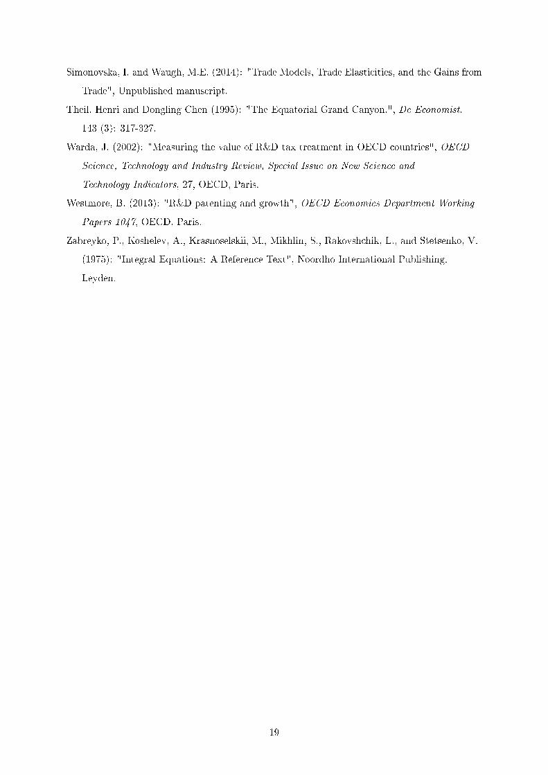
3 Calibration of Key Model Parameters

To compute the quantitative multi-region equilibrium for each time period from a given year

to the steady state (long run), we need the parameters contained in the equations above and

summarized in Table 1. Apart from parameters that are common to all regions and region-

specic land endowments which are given in the data, these are initial productivity levels in

production for all regions and trade costs between all pairs of regions.3 Table 1 alludes to the

sources of these parameters, some of which are collected from other work and some of which are

derived (computed or estimated) here.

Table 1 about here

We organize the remainder of this section in subsections which pertain to important model

blocks based on which estimating equations are formulated or key parameters can be backed

out.1A detailed derivation of this equilibrium condition is presented Appendix C.1.2A detailed derivation of the growth rate of aggregate welfare is presented in Appendix C.2.3Initial productivity levels, τ0, are obtained using the structure of the model and observed population and

wage levels in year 2005. Technical details on the derivation of τ0 are explained in Appendix A.

7

3.1 Delineation of Regions and Land Endowments

The delineation of regions used in our analysis is dictated by the denitions used in regional

patent-statistical database (REGPAT) of the Organization of Economic Cooperation and De-

velopment (OECD).4 In 2005, REGPAT distinguishes 5,633 regions across 213 countries around

the globe. The size of regions by land mass (somewhat less so by income or patenting) diers

to a large extent. In some countries the granularity of regions is very ne, while it is coarse

in others. In some cases, even a whole country is a region (e.g., in some African or Asian and

South American countries). This pattern is related to the intensity of patenting in a country:

economies with more patents tend to be delineated in a more ne-grained fashion, while the

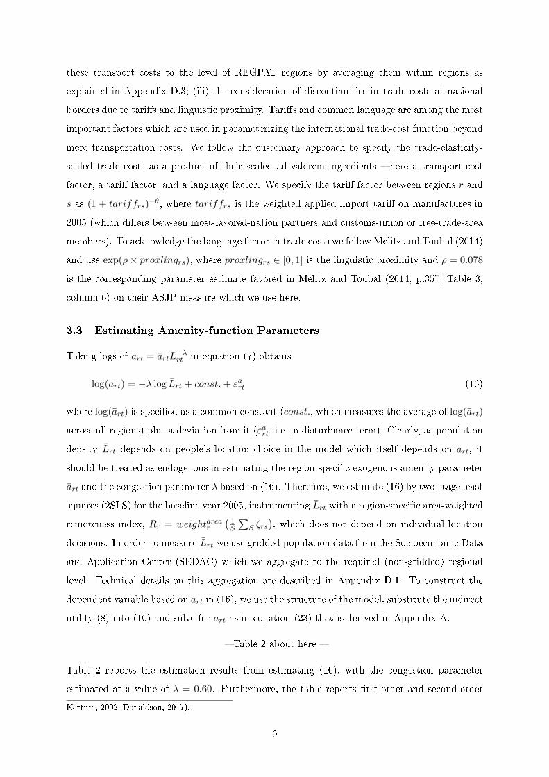
ones with less patenting tend to be more coarsely captured. Figure 1 shows a world map of

all regions that indicates all countries in the sample with a red color and countries not part of

the sample with a white color. In the gure, country borders are drawn in blue and regional

borders in yellow. Whenever region and country borders coincide, the yellow region borders are

not visible.

Figure 1 about here

The map shows that most of the regions are in North America (United States, Canada and

Mexico) and Europe, which together constitute 90 percent of the regions in the data. Using

the regional code in the REGPAT database we can link the REGPAT regions with spatial

information from two sources: (i) we employ the Geographical Information and Maps (GISCO)

database from eurostat for spatial information on European countries (NUTS3 regions, 2010)

and (ii) we use the Global Administrative Areas (GADM) spatial database on administrative

boundaries for all other countries. Then, we extract the land mass for each region using ArcGIS

software after excluding water sheds within the boundaries of a region. We normalize the region-

specic land mass by the average landmass, 1S

∑Sr=1Gr.

3.2 Trade-cost-function Parameters

In constructing trade costs, we employ three ingredients: (i) fast-marching-algorithm-based

transportation costs between pairs of 1 grid cells along the lines of Desmet et al. (2017) and

using passing-through parameters from Allen and Arkolakis (2014);5 (ii) a correspondence of

4The REGPAT database links the Worldwide Statistical Patent Database (PATSTAT) from the European

Patent Oce (EPO) to more that 5,500 regions across the globe, utilizing the addresses of the applicants and

inventors.5We modify those costs by symmetrifying them (using the average for costs from A to B and B to A) and by

assuming that intra-cell transport costs are (essentially) zero as is customary in Ricardian work (see Eaton and

8

these transport costs to the level of REGPAT regions by averaging them within regions as

explained in Appendix D.3; (iii) the consideration of discontinuities in trade costs at national

borders due to taris and linguistic proximity. Taris and common language are among the most

important factors which are used in parameterizing the international trade-cost function beyond

mere transportation costs. We follow the customary approach to specify the trade-elasticity-

scaled trade costs as a product of their scaled ad-valorem ingredients here a transport-cost

factor, a tari factor, and a language factor. We specify the tari factor between regions r and

s as (1 + tariffrs)−θ, where tariffrs is the weighted applied import tari on manufactures in

2005 (which diers between most-favored-nation partners and customs-union or free-trade-area

members). To acknowledge the language factor in trade costs we follow Melitz and Toubal (2014)

and use exp(ρ× proxlingrs), where proxlingrs ∈ [0, 1] is the linguistic proximity and ρ = 0.078

is the corresponding parameter estimate favored in Melitz and Toubal (2014, p.357, Table 3,

column 6) on their ASJP measure which we use here.

3.3 Estimating Amenity-function Parameters

Taking logs of art = artL−λrt in equation (7) obtains

log(art) = −λ log Lrt + const.+ εart (16)

where log(art) is specied as a common constant (const., which measures the average of log(art)

across all regions) plus a deviation from it (εart, i.e., a disturbance term). Clearly, as population

density Lrt depends on people's location choice in the model which itself depends on art, it

should be treated as endogenous in estimating the region-specic exogenous amenity parameter

art and the congestion parameter λ based on (16). Therefore, we estimate (16) by two-stage least

squares (2SLS) for the baseline year 2005, instrumenting Lrt with a region-specic area-weighted

remoteness index, Rr = weightarear

(1S

∑S ζrs

), which does not depend on individual location

decisions. In order to measure Lrt we use gridded population data from the Socioeconomic Data

and Application Center (SEDAC) which we aggregate to the required (non-gridded) regional

level. Technical details on this aggregation are described in Appendix D.1. To construct the

dependent variable based on art in (16), we use the structure of the model, substitute the indirect

utility (8) into (10) and solve for art as in equation (23) that is derived in Appendix A.

Table 2 about here

Table 2 reports the estimation results from estimating (16), with the congestion parameter

estimated at a value of λ = 0.60. Furthermore, the table reports rst-order and second-order

Kortum, 2002; Donaldson, 2017).

9

moments of art. As described above, the region-specic exogenous amenity attribute is dened

as art ≡ exp(const.+ εart). In the general-equilibrium analysis, art is kept constant for all timeperiods.

3.4 Technology and Productivity-evolution Parameters

Table 1 summarizes the assumed values of the technology parameters α, θ, µ and the productivity-

evolution parameters ξ, ν which we take from others' work. Here, we focus on the two remain-

ing parameters γ1, γ2 which are elemental but for which existing estimates are not available

given the adopted model structure. Specically, the BGP implies the relationship in equation

(15). Taking logs and discretizing (15) obtains

log(urt+1)− log(urt) = log(yrt+1)− log(yrt)

=(1− γ2)

θlog(η) +

γ1

ξlog(Ψ) +

1− γ2

θlog(

∑r

L∗rt)(17)

where Ψ ≡ γ1/νγ1+µξ , S = 5, 633, and L∗rt ≡

[Lrthrt

] θγ1(1−γ2)ξ . Note that equation (17) depends on

both population density (Lrt) as well as on real-income data (yrt+1, yrt). Either type of data is

available at the 1 by 1 resolution from the G-Econ 4.0 Research Project at Yale University,

which we aggregate to the required (non-gridded) regional level as described in Appendix D.2.6

We use the mentioned data for t ∈ 1990, 1995, 2000 and t + 1 ∈ 1995, 2000, 2005 and

approximate the log dierence between years t + 1 and t by a ve-year interval. Moreover, we

determine γ1, γ2 by pooling the data for the mentioned three year tuples t, t+ 1.

For the estimation of γ1, γ2, note that γ1, γ2 ∈ (0, 1) and that hrt and, hence, L∗rt itself depends

on γ1. However, using the notion of a bivariate bounded parameter space, we can search for the

optimal values of γ1, γ2 by doing a grid search on the bivariate unit interval, employing the

respective value of hrt(γ1). It will become clear in the subsequent subsection how hrt depends

on γ1. Adopting this procedure, we obtain the estimates γ1 = 0.273 and γ2 = 0.9897 listed in

Table 1.

6Notice that we do have population data from two sources, namely SEDAC and the G-Econ 4.0 Research

Project. Whereas SEDAC provides gridded population data with an output solution of 30 arc-seconds (approx.

1km at the equator), the G-Econ project provides the same data on an aggregated 1 by 1 resolution. For

consistency reasons, we inform the estimating equation based on (17) by population and real-income data from

the G-Econ 4.0 Research Project. For all other applications, we use population data from SEDAC directly, to

avoid measurement error from aggregation.

10

3.5 Estimation of hrt (preliminary)

We structurally estimate hrt using (6) and knowing (5). To link the available data to our model,

we assume φξrt = Patentsξrt, so that

φξrt = Patentsξrt =γ1

ξν[µ+ γ1/ξ]Lrthrt (18)

where Patentsrt are registered patents per unit of land in region r at year t from REGPAT.7

Here, Lrt is the population density in region r at year t, where population levels are taken from

SEDAC and aggregated to the regional level. We parametrize hrt as

hrt = exp(Drtβ + |latr|Drtγ) (19)

whereDrt describes a vector of binary R&D-policy indicators from Boesenberg and Egger (2016).

The indicators inDrt are country-year-specic and each region r is associated with a single coun-

try. The indicators include a binary indicator variable for partial exemptions of returns on R&D

investments, also known as patent boxes (Dpatentboxrt), R&D investment related grants from

the government (Dgrantsrt), tax credit on R&D investments (Dtaxcreditrt), tax holidays for

rms with R&D investment (Dtaxholidayrt), super deductions of more than 100% for R&D

investments from prots (Dsuperdrt), any form of deductions of R&D investments from prof-

its other than super deductions (Ddeducrt), and a lower eective average tax rate on R&D

investments as compared to non-R&D-related investments (Deatrrdrt). Deatrrdrt is coded as

a nonlinear combination of the other front-end R&D-policy instruments (i.e., the instruments

except Dpatentboxrt), as it takes on the maximum value for each rt across all the respective

instruments. Hence, whenever there is any front-end instrument in place, Deatrrdrt is unity.

Additionally, we include an interaction term of each binary R&D policy indicator with the abso-

lute value of the latitude of the region's centroid (|latr|Drt) for two reasons. First, it allows us to

account for dierences on how productively a region in terms of its distance to the equator can

use an adopted R&D policy instrument. Notable contributions that have highlighted a relation

between a rm's ability to adopt new technologies and its distance to the equator are Theil and

Chen (1995) and Hall and Jones (1997), among others. And second, it adds variation in the

marginal eect of policy instruments across regions.

We refrain from explicitly modeling any budgetary eects of the considered R&D policy in-

struments for the following reason. The employed instruments aect the marginal tax rate on

returns generated from R&D in a highly nonlinear way. However, as countries do not report

7Coelli et al. (2016) provide evidence that patenting can be understood as innovation as they nd an increasing

citation rate of registered patents over time.

11

specic tax revenues generated from such investments, it is not possible to validate a structural

form of the associated nonlinear relationship. From this perspective, it appears customary to

resort to a reduced-form nexus between the instruments and patenting and consider treatment

eects of the instruments based on this reduced-form nexus by embedding it in the structure of

the general equilibrium model.

Reformulating a stochastic version of (18) in terms of an exponential-family-model specication,

we arrive at

Patentsrt = exp(β0 +1

ξlog ˜Lrt +

1

ξlog hrt + εrt) (20)

where ˜Lrt= γ1/ξν[µ+ γ1/ξ]Lrt and εrt is the error term. As the location decision of individuals

may be endogenous to innovation potential of the region, we instrument ˜Lrt with the unweighted

average trade costs through a control function approach. After substituting log(hrt) with (Drtβ+

|latrt|Drtγ) according to (19), we estimate (20) to obtain the parameter estimates β0, 1/ξ, β, γ

using a cross section of the data for the baseline year t = 2005 and negative binomial regression.8

Given the parameter estimates we obtain an estimate of hrt for each region r in 2005 as

hrt = exp(Drtβ + |latr|Drtγ) (21)

and hrt is kept constant for each period in the general-equilibrium analysis.

In Table 3, we summarize all variables which inform this procedure. The table is organized in

three vertical blocks: the one at the top provides information on patents; the one in the center

summarizes moments of the land and population distribution as well as log( ˜Lrt) which combines

the two; and the block at the bottom summarizes the elements of Drt as well as |latr| used in

|latr|Drt, underlying the parametrization of hrt.

Table 3 about here

The gures on patent registrations at the top of Table 3 are expressed in normalized units of

land, Gr. The two lines at the top of the respective block pertain to a regional denomination

of patents according to the residence of inventors (inv), whereas the two lines at the bottom of

the respective block pertain to a regional denomination of patents according to the residence

of applicants (app). For each concept, we report the average normalized patent registration

counts for 2005 as well as for the average year in 2000-2010. While for the average year zero-

registration events are scarcer than for a single year such as 2005, the average value of patents

8The negative binomial model accommodates the present over-dispersion of the data, whereby the variance in

patents increases with the conditional mean.

12

is smaller than in the center of the time interval due to the surge of patenting. Moreover, the

respective gures suggest that inventions are more dispersed than applications (i.e., applications

are more concentrated). This pattern is shown in higher rst as well as second moments of

patent applications. The latter shows also in a higher frequency of zeros in the applications data

than the inventions data, which is not obvious from the table.

While the information about the population and land data may be interesting to some readers, we

suppress a discussion here for the sake of brevity and rather focus on the R&D-policy instruments

used in the parametrization of hrt. The respective indicators all of which are measured in 2005

suggest that almost all regions r are exposed to some type of R&D-policy instrument, as

their eective tax rate on R&D-related prots is lower than the one on non-R&D-related prots

(Deatrrdr). Moreover, more than two-thirds of the regions operate under a regime with tax

credits (Dtaxcreditr). Other R&D-policy instruments are used much less frequently (by fewer

countries or by countries with not very ne-grained regions). For example, a grants system is

applied in only about eight percent of the regions, super deductions in only about ve percent

of the regions, and deductions, tax holidays and patent boxes in only about two to three percent

of the regions.

The parameter estimates and some other statistics based on the aforementioned procedure and

data are summarized in Table 4.

Table 4 about here

In Table 4, we report on marginal eects of the covariates in (20) for four specications. The

ones numbered (1)-(2) pertain to inventor-based patents per region the average year in 2000-

2010 while the ones numbered (3)-(4) pertain to applicant-based ones.9 In columns (1) and (3)

we set γ = 0 (interaction terms with |latr| are excluded) while we abandon this restriction in

columns (2) and (4). Apart from marginal eects of ˜Lrt as well as individual elements in Drt we

report the model t through the correlation of the data with the model prediction on log(hrt)

as well as the number of observations (regions) used.

The results suggest that more densely populated regions (i.e., the ones with higher values of ˜Lrt)

display higher counts of patent inventions as well as applications. Tax holidays (Dtaxholidaysr)

and grants (Dgrantsr) tend to raise patent counts, while patent boxes (Dpatentboxr; a back-end

incentive which primarily promotes the ownership but not the invention of patents) reduce patent

registrations. A reduction of the eective average tax rate on R&D-investment-based relative to

9We choose patent registrations for the average year in 2000-2010 as a dependent variable in all specications

reported in Table 4 to account for the time it takes to get a patent ling granted.

13

other investments benets patent registrations (Deatrrdr; in particular, for inventions).10 Also

regular deductions (Ddeducr) of R&D investments from prots display a positive eect on patent

registrations. Overall, the explanatory power of the model is relatively high, as can be seen from

the correlation coecient between log(Patentsrt) and log( Patentsrt) in the table.11 In what

follows, we will use the specication in column (2) as the preferred model, since the explanatory

power is relatively high and there is variation in the marginal eect of policy instruments across

regions.

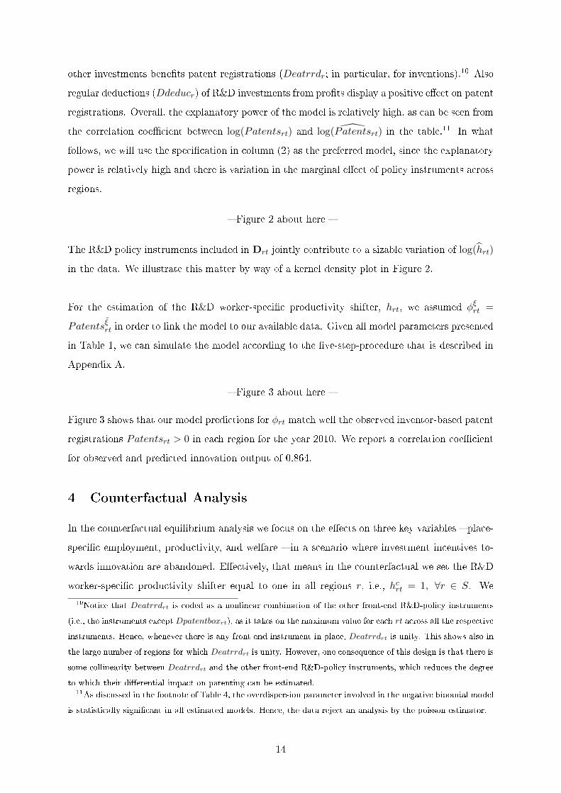
Figure 2 about here

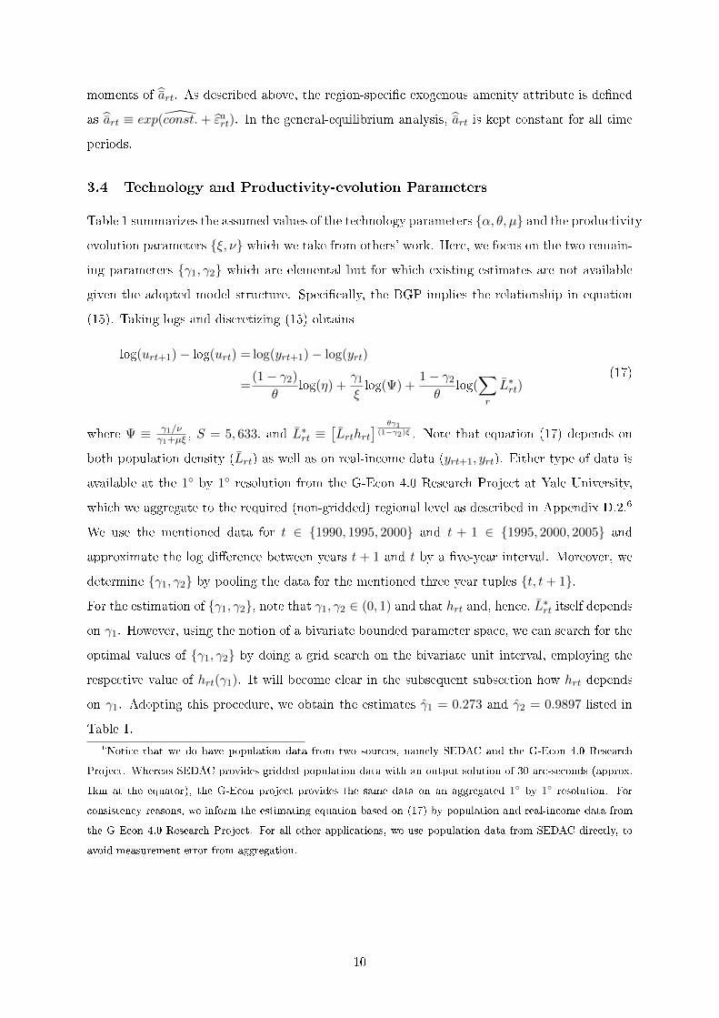
The R&D policy instruments included in Drt jointly contribute to a sizable variation of log(hrt)

in the data. We illustrate this matter by way of a kernel density plot in Figure 2.

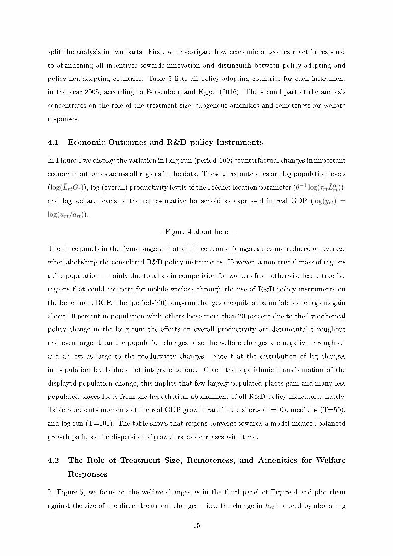
For the estimation of the R&D worker-specic productivity shifter, hrt, we assumed φξrt =

Patentsξrt in order to link the model to our available data. Given all model parameters presented

in Table 1, we can simulate the model according to the ve-step-procedure that is described in

Appendix A.

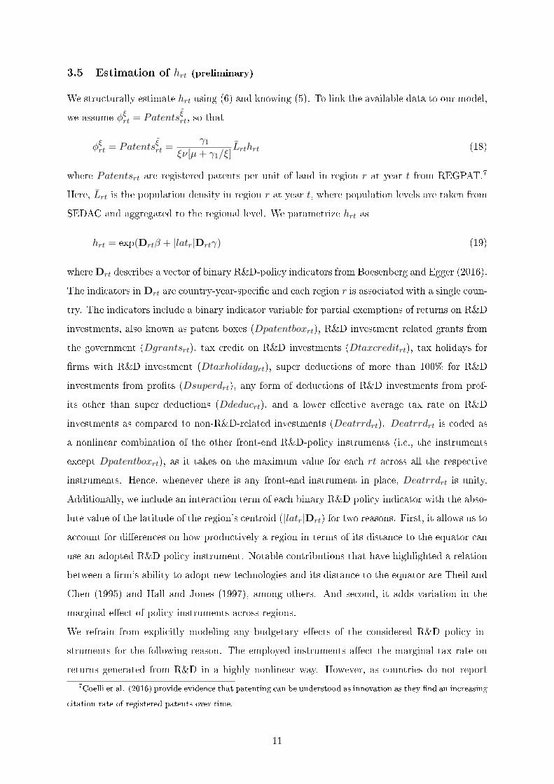
Figure 3 about here

Figure 3 shows that our model predictions for φrt match well the observed inventor-based patent

registrations Patentsrt > 0 in each region for the year 2010. We report a correlation coecient

for observed and predicted innovation output of 0.864.

4 Counterfactual Analysis

In the counterfactual equilibrium analysis we focus on the eects on three key variables place-

specic employment, productivity, and welfare in a scenario where investment incentives to-

wards innovation are abandoned. Eectively, that means in the counterfactual we set the R&D

worker-specic productivity shifter equal to one in all regions r, i.e., hcrt = 1, ∀r ∈ S. We

10Notice that Deatrrdrt is coded as a nonlinear combination of the other front-end R&D-policy instruments

(i.e., the instruments except Dpatentboxrt), as it takes on the maximum value for each rt across all the respective

instruments. Hence, whenever there is any front-end instrument in place, Deatrrdrt is unity. This shows also in

the large number of regions for which Deatrrdrt is unity. However, one consequence of this design is that there is

some collinearity between Deatrrdrt and the other front-end R&D-policy instruments, which reduces the degree

to which their dierential impact on patenting can be estimated.11As discussed in the footnote of Table 4, the overdispersion parameter involved in the negative binomial model

is statistically signicant in all estimated models. Hence, the data reject an analysis by the poisson estimator.

14

split the analysis in two parts. First, we investigate how economic outcomes react in response

to abandoning all incentives towards innovation and distinguish between policy-adopting and

policy-non-adopting countries. Table 5 lists all policy-adopting countries for each instrument

in the year 2005, according to Boesenberg and Egger (2016). The second part of the analysis

concentrates on the role of the treatment-size, exogenous amenities and remoteness for welfare

responses.

4.1 Economic Outcomes and R&D-policy Instruments

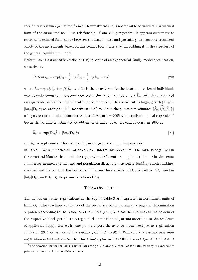
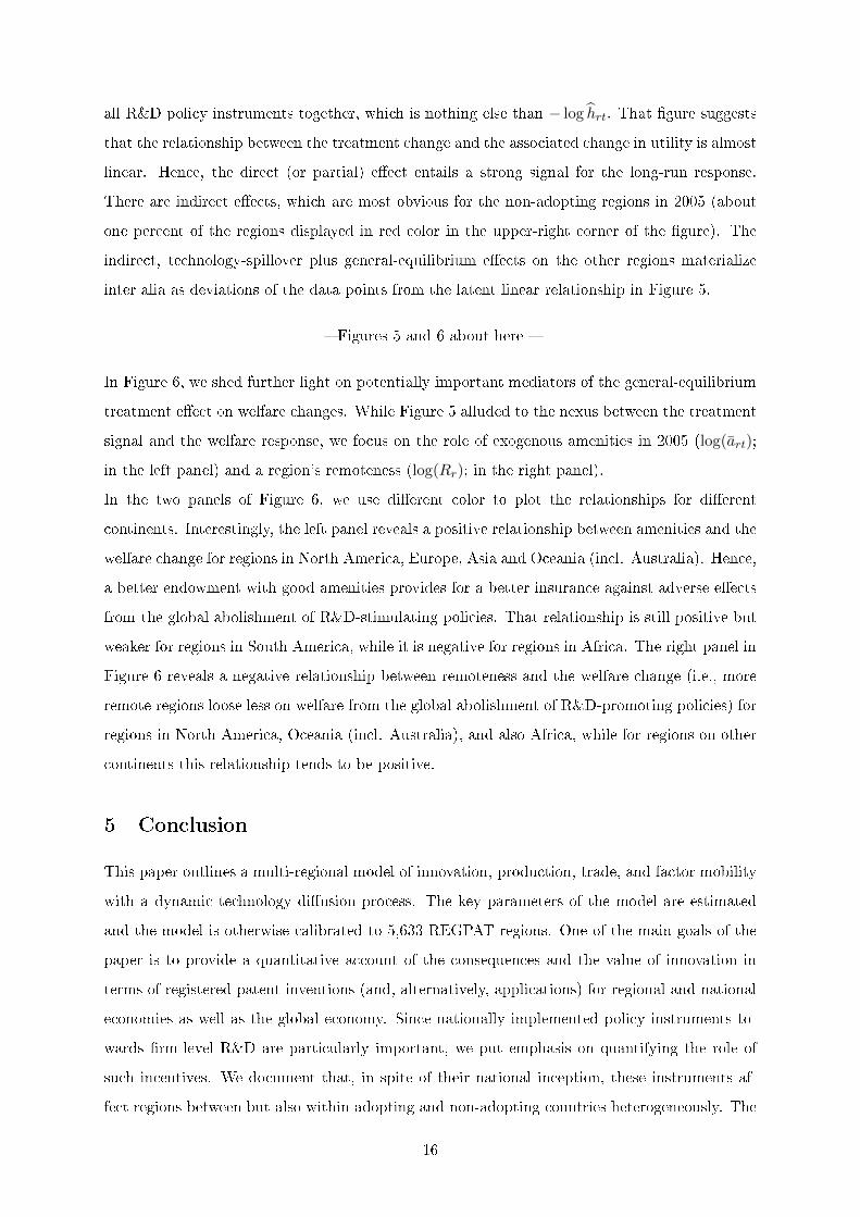
In Figure 4 we display the variation in long-run (period-100) counterfactual changes in important

economic outcomes across all regions in the data. These three outcomes are log population levels

(log(LrtGr)), log (overall) productivity levels of the Fréchet location parameter (θ−1 log(τrtL

αrt)),

and log welfare levels of the representative household as expressed in real GDP (log(yrt) =

log(urt/art)).

Figure 4 about here

The three panels in the gure suggest that all three economic aggregates are reduced on average

when abolishing the considered R&D policy instruments. However, a non-trivial mass of regions

gains population mainly due to a loss in competition for workers from otherwise less attractive

regions that could compete for mobile workers through the use of R&D policy instruments on

the benchmark BGP. The (period-100) long-run changes are quite substantial: some regions gain

about 10 percent in population while others loose more than 20 percent due to the hypothetical

policy change in the long run; the eects on overall productivity are detrimental throughout

and even larger than the population changes; also the welfare changes are negative throughout

and almost as large to the productivity changes. Note that the distribution of log changes

in population levels does not integrate to one. Given the logarithmic transformation of the

displayed population change, this implies that few largely populated places gain and many less

populated places loose from the hypothetical abolishment of all R&D policy indicators. Lastly,

Table 6 presents moments of the real GDP growth rate in the short- (T=10), medium- (T=50),

and log-run (T=100). The table shows that regions converge towards a model-induced balanced

growth path, as the dispersion of growth rates decreases with time.

4.2 The Role of Treatment Size, Remoteness, and Amenities for Welfare

Responses

In Figure 5, we focus on the welfare changes as in the third panel of Figure 4 and plot them

against the size of the direct treatment changes i.e., the change in hrt induced by abolishing

15

all R&D policy instruments together, which is nothing else than − log hrt. That gure suggests

that the relationship between the treatment change and the associated change in utility is almost

linear. Hence, the direct (or partial) eect entails a strong signal for the long-run response.

There are indirect eects, which are most obvious for the non-adopting regions in 2005 (about

one percent of the regions displayed in red color in the upper-right corner of the gure). The

indirect, technology-spillover plus general-equilibrium eects on the other regions materialize

inter alia as deviations of the data points from the latent linear relationship in Figure 5.

Figures 5 and 6 about here

In Figure 6, we shed further light on potentially important mediators of the general-equilibrium

treatment eect on welfare changes. While Figure 5 alluded to the nexus between the treatment

signal and the welfare response, we focus on the role of exogenous amenities in 2005 (log(art);

in the left panel) and a region's remoteness (log(Rr); in the right panel).

In the two panels of Figure 6, we use dierent color to plot the relationships for dierent

continents. Interestingly, the left panel reveals a positive relationship between amenities and the

welfare change for regions in North America, Europe, Asia and Oceania (incl. Australia). Hence,

a better endowment with good amenities provides for a better insurance against adverse eects

from the global abolishment of R&D-stimulating policies. That relationship is still positive but

weaker for regions in South America, while it is negative for regions in Africa. The right panel in

Figure 6 reveals a negative relationship between remoteness and the welfare change (i.e., more

remote regions loose less on welfare from the global abolishment of R&D-promoting policies) for

regions in North America, Oceania (incl. Australia), and also Africa, while for regions on other

continents this relationship tends to be positive.

5 Conclusion

This paper outlines a multi-regional model of innovation, production, trade, and factor mobility

with a dynamic technology diusion process. The key parameters of the model are estimated

and the model is otherwise calibrated to 5,633 REGPAT regions. One of the main goals of the

paper is to provide a quantitative account of the consequences and the value of innovation in

terms of registered patent inventions (and, alternatively, applications) for regional and national

economies as well as the global economy. Since nationally implemented policy instruments to-

wards rm-level R&D are particularly important, we put emphasis on quantifying the role of

such incentives. We document that, in spite of their national inception, these instruments af-

fect regions between but also within adopting and non-adopting countries heterogeneously. The

16

degree of heterogeneity depends on the extent of the treatment how many and which instru-

ments are used and how productively a region in terms of its distance to the equator can use

them. Moreover, the degree of heterogeneity depends on other fundamentals such as a region's

integration in the national and international transport network as well as its attractiveness for

the location of mobile labor in terms of the available amenities.

One important insight is that the use of policy instruments which are designed to stimulate

private R&D are globally benecial in terms of productivity and welfare. In other words, also

countries and their regions who do not use such instruments benet from their use abroad due

to technology spillovers. However, adopting countries and regions benet signicantly more

strongly. Also, the long-run relocation eects are substantial: some regions gain about 10 per-

cent in population while others loose more than 20 percent due to a hypothetical abolishment of

all R&D policy instruments. This is mainly due a loss in competition for workers from otherwise

less attractive regions, which could compete for mobile workers through the use of R&D policy

instruments.

Furthermore, the quantitative analysis suggests that particularly regions with high amenities

and a low degree of transport remoteness tend to benet from such policy instruments, as they

are able to attract labor which is key not only for production but also innovation, and as they

can generate a high return on innovations to rms through their greater global market potential.

This result is especially true for regions in North America and Oceania, whereas the eect is

less predominant in Europe or Asia.

17

References

Allen, T. and C. Arkolakis (2014): "Trade and the Topography of the Spatial Economy",

The Quarterly Journal of Economics, 129(3), 1085-1140.

Baumann, M., B. Knoll, and N. Riedel (2014): "The global eects of R&D tax incentives:

evidence from micro-data", Unpublished manuscript.

Bernard, A.B., Eaton, J., Jensen, J.B., and Kortum, S. (2003): "Plants and Productivity

in International Trade", American Economic Review, 93(4), 1268-1290.

Boesenberg, S. and P. H. Egger (2016): "R&D tax incentives and the emergence and trade

of ideas", Economic Policy, 89, 32.

Carlino, G., Chatterjee, S., and Hunt R. (2007): "Urban Density and the Rate of Invention",

Journal of Urban Economics, 61, 389-419.

Coelli F., A. Moxnes and K. H. Ulltveit-Moe (2016): "Better, Faster, Stronger:

Global Innovation and Trade Liberalization," NBER Working Papers 22647,

National Bureau of Economic Research, Inc.

Desmet, K., D. K. Nagy, and E. Rossi-Hansberg (2017): "The Geography of Development",

Journal of Political Economy (forthcoming).

Desmet, K. and Rappaport, J. (2015): "The Settlement of the United States, 1800 to 2000:

The Long Transition Towards Gibrat's Law", Journal of Urban Economics, 98, 50-68 .

Desmet, K. and Rossi-Hansberg, E. (2015): "On the Spatial Economic Impact of Global

Warming", Journal of Urban Economics, 88, 16-37.

Donaldson, D. (2017): "Railroads of the Raj: Estimating the Impact of Transportation

Infrastructure", American Economic Review (forthcoming).

Eaton, J. and Kortum, S. (2002): "Technology, Geography, and Trade", Econometrica, 70(5),

1741-1779.

Greenwood, J., Hercowitz, Z., and Krusell, P. (1997): "Long-Run Implications of Invest-

ment-Specic Technological Change", American Economic Review, 87(3), 342-362.

Hall, Robert E., Charles I. Jones (1997): "Levels of Economic Activity Across Countries.",

American Economic Review, 87 (2): 173-177.

Melitz, J. and Toubal,F. (2014): "Native Language, Spoken Language, Translation and Trade",

Journal of International Economics, 93(2), 351-363.

Monte, F., Redding, S. and Rossi-Hansberg, E. (2015): "Commuting, Migration and Local

Employment Elasticities", NBER Working Paper #21706.

18

Simonovska, I. and Waugh, M.E. (2014): "Trade Models, Trade Elasticities, and the Gains from

Trade", Unpublished manuscript.

Theil, Henri and Dongling Chen (1995): "The Equatorial Grand Canyon.", De Economist,

143 (3): 317-327.

Warda, J. (2002): "Measuring the value of R&D tax treatment in OECD countries", OECD

Science, Technology and Industry Review, Special Issue on New Science and

Technology Indicators, 27, OECD, Paris.

Westmore, B. (2013): "R&D patenting and growth", OECD Economics Department Working

Papers 1047, OECD, Paris.

Zabreyko, P., Koshelev, A., Krasnoselskii, M., Mikhlin, S., Rakovshchik, L., and Stetsenko, V.

(1975): "Integral Equations: A Reference Text", Noordho International Publishing.

Leyden.

19

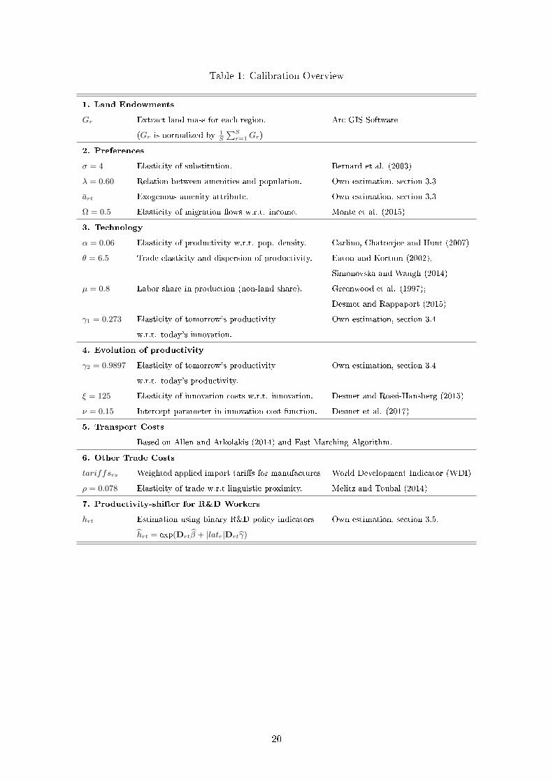
Table 1: Calibration Overview

1. Land Endowments

Gr Extract land mass for each region. Arc GIS Software

(Gr is normalized by 1S

∑Sr=1 Gr)

2. Preferences

σ = 4 Elasticity of substitution. Bernard et al. (2003)

λ = 0.60 Relation between amenities and population. Own estimation, section 3.3

art Exogenous amenity attribute. Own estimation, section 3.3

Ω = 0.5 Elasticity of migration ows w.r.t. income. Monte et al. (2015)

3. Technology

α = 0.06 Elasticity of productivity w.r.t. pop. density. Carlino, Chatterjee and Hunt (2007)

θ = 6.5 Trade elasticity and dispersion of productivity. Eaton and Kortum (2002),

Simonovska and Waugh (2014)

µ = 0.8 Labor share in production (non-land share). Greenwood et al. (1997);

Desmet and Rappaport (2015)

γ1 = 0.273 Elasticity of tomorrow's productivity Own estimation, section 3.4

w.r.t. today's innovation.

4. Evolution of productivity

γ2 = 0.9897 Elasticity of tomorrow's productivity Own estimation, section 3.4

w.r.t. today's productivity.

ξ = 125 Elasticity of innovation costs w.r.t. innovation. Desmet and Rossi-Hansberg (2015)

ν = 0.15 Intercept parameter in innovation cost function. Desmet et al. (2017)

5. Transport Costs

Based on Allen and Arkolakis (2014) and Fast Marching Algorithm.

6. Other Trade Costs

tariffsrs Weighted applied import taris for manufactures World Development Indicator (WDI)

ρ = 0.078 Elasticity of trade w.r.t linguistic proximity. Melitz and Toubal (2014)

7. Productivity-shifter for R&D Workers

hrt Estimation using binary R&D policy indicators Own estimation, section 3.5.

hrt = exp(Drtβ + |latr|Drtγ)

20

Table 2: Amenity Parameter Estimation

Regressor Parameter Coe. Moments of ar ≡ exp(const.+ εar)

(Std. err.)

First Stage: Dep. Var. log (Lrt) Mean Std. Dev.

log(Rr) ρ1 -0.473*** 63,314 373,515

(0.014)

Second Stage: Dep. Var. log(art) 5% 10% 50% 90% 95%

log (Lr) −λ -0.600*** 203.4 461.9 6,563.9 81,232.7 165,393.5

(0.033)

#obs 5,633

Table 3: Summary Statistics

Variable Mean Std. Dev. Min. Max.

Patents per norm. unit of land

Patentsrt (inv) 2005 800.98 5,366.5 0 205,728.4

Patentsrt (inv) avg 2000-2010 775.97 5104.1 0 196,549.3

Patentsrt (app) 2005 1,154.44 13,781.7 0 617,404.1

Patentsrt (app) avg 2000-2010 1,124.27 13,563.3 0 610,453.4

Gr 1 11.83 1.9e-04 624.27

LrtGr 1,108,491 7,637,692 5 2.17e+08

log( ˜Lrt) 9.89 2.01 -0.428 16.44

R&D-policy indicators

Dtaxcreditrt 0.715 0.452 0 1

Dsuperdrt 0.053 0.224 0 1

Dtaxholidayrt 0.023 0.151 0 1

Dgrantsrt 0.081 0.273 0 1

Dpatentboxrt 0.022 0.147 0 1

Ddeducrt 0.029 0.169 0 1

Deatrrdrt 0.982 0.131 0 1

|latr| 40.205 9.583 0.2 74.728

Notes: Patentsrt(inv) refers to a regional denomination of patents according to the residence of inventors

(inv). Patentsrt(app) refers to a regional denomination of patents according to the residence of applicants

(app).

21

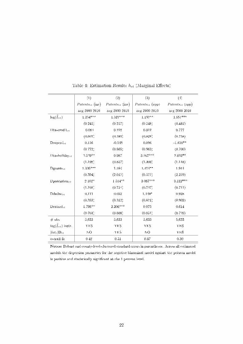
Table 4: Estimation Results hrt (Marginal Eects)

(1) (2) (3) (4)

Patentsrt (inv) Patentsrt (inv) Patentsrt (app) Patentsrt (app)

avg 2000-2010 avg 2000-2010 avg 2000-2010 avg 2000-2010

log( ˜Lrt) 1.254*** 1.527*** 1.197** 1.557***

(0.245) (0.257) (0.548) (0.481)

Dtaxcreditrt -0.084 0.218 0.312 0.777

(0.601) (0.593) (0.828) (0.758)

Dsuperdrt 0.156 -0.148 0.096 -1.650**

(0.772) (0.865) (0.963) (0.700)

Dtaxholidayrt 2.529** 0.987 3.167*** 2.023**

(1.198) (0.857) (1.200) (1.148)

Dgrantsrt 1.336*** 1.594 1.474** 1.944

(0.394) (2.017) (0.577) (2.259)

Dpatentboxrt -2.102* -1.514** -3.087*** -3.122***

(1.168) (0.754) (0.747) (0.711)

Ddeducrt 0.111 0.032 1.449* 0.928

(0.333) (0.312) (0.871) (0.902)

Deatrrdrt 1.798** 2.206*** 0.075 0.614

(0.763) (0.800) (0.951) (0.729)

# obs 5,633 5,633 5,633 5,633

log( ˜Lrt) instr. YES YES YES YES

|latr|Drt NO YES NO YES

overall t 0.42 0.51 0.37 0.30

Notes: Robust and county-level-clustered standard errors in parentheses. Across all estimated

models the dispersion parameter for the negative binominal model against the poisson model

is positive and statistically signicant at the 1 percent level.

22

Table 5: R&D Policy Instruments in 2005

R&D Policy Instrument Description Countries (in 2005)

Dtaxcreditrt Tax credits on R&D investments Austria, Canada, China, France, Ireland, Japan,

Mexico, Netherlands, Norway, Portugal, South Korea,

Spain, Taiwan, US, Venezuela.

Dtaxholidayrt Tax holidays for rms with R&D investments. France, Malaysia, Singapore, Switzerland.

Dgrantsrt R&D investment related grants from the government. Germany, Hungary, Ireland, Israel.

Dpatentboxrt (Partial) exemption of returns on R&D investments. France, Hungary.

Ddeducrt Any form of deductions on R&D investments. Australia, Belgium, Ireland, Japan, South Korea.

Dsuperdrt Super deductions of more than 100% Australia, China, Czech Republic, Hungary, India,

for R&D investments. Malaysia, Malta, Puerto Rico, Singapore, UK.

Deatrrdrt Eective average tax rate is lower on returns on 114 of 213 countries in the data.

R&D investments than on other investments.

France incl. Guadeloupe, French Guiana, Martinique, Reunion; Netherlands incl. Bonaire; US incl. American Samoa, US Minor Outlying Islands; Australia incl. Cocos

Islands; UK incl. Falkland Islands, Gibraltar, Montserrat, Pitcarn, St. Helena.

Table 6: Moments of Real GDP Growth

Period Min Max Mean Std

T=10 0.010 0.050 0.033 0.003

T=50 0.015 0.043 0.032 0.002

T=100 0.02 0.038 0.031 0.001

23

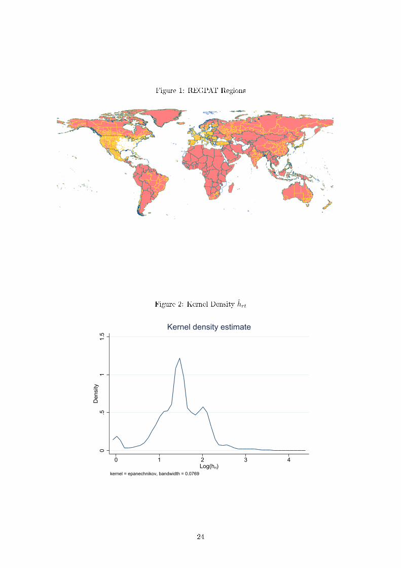
Figure 1: REGPAT Regions

Figure 2: Kernel Density hrt

0.5

11.

5D

ensi

ty

0 1 2 3 4Log(hrt)

kernel = epanechnikov, bandwidth = 0.0769

Kernel density estimate

24

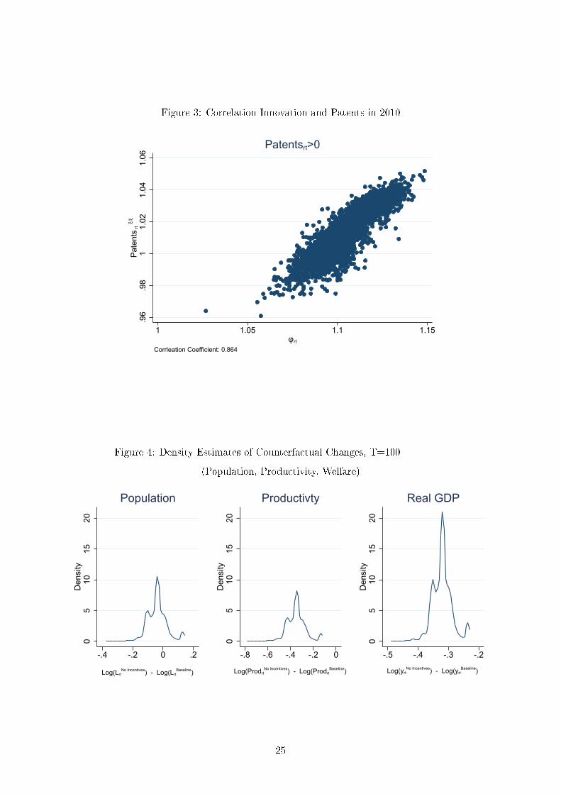
Figure 3: Correlation Innovation and Patents in 2010

.96

.98

11.

021.

041.

06Pa

tent

s rt ξ/

ξ

1 1.05 1.1 1.15φ rt

Corrleation Coefficient: 0.864

Patentsrt>0

Figure 4: Density Estimates of Counterfactual Changes, T=100

(Population, Productivity, Welfare)

05

1015

20D

ensi

ty

-.4 -.2 0 .2

Log(LrtNo Incentives) - Log(Lrt

Baseline)

Population

05

1015

20D

ensi

ty

-.8 -.6 -.4 -.2 0

Log(ProdrtNo Incentives) - Log(Prodrt

Baseline)

Productivty

05

1015

20D

ensi

ty

-.5 -.4 -.3 -.2

Log(yrtNo Incentives) - Log(yrt

Baseline)

Real GDP

25

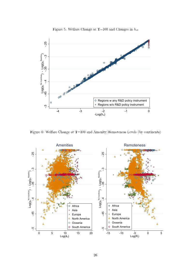
Figure 5: Welfare Change at T=100 and Changes in hrt

-.5-.4

5-.4

-.35

-.3-.2

5Lo

g(y r

tNo

Ince

ntiv

es)

- Lo

g(y r

tBase

line )

-4 -3 -2 -1 0-Log(hrt)

Regions w any R&D policy instrumentRegions w/o R&D policy instrument

Figure 6: Welfare Change at T=100 and Amenity/Remoteness Levels (by continents)

-.5-.4

5-.4

-.35

-.3-.2

5Lo

g(y r

tNo

Ince

ntiv

es)

- Lo

g(y r

tBase

line )

0 5 10 15 20Log(ārt)

AfricaAsiaEuropaNorth AmericaOceaniaSouth America

Amenities

-.5-.4

5-.4

-.35

-.3-.2

5Lo

g(y r

tNo

Ince

ntiv

es)

- Lo

g(y r

tBase

line )

-15 -10 -5 0 5Log(Rr)

AfricaAsiaEuropaNorth AmericaOceaniaSouth America

Remoteness

26

Appendix

A Simulation of the Model

The simulation of the model proceeds as follows.

First, we identify the initial eciency distribution τ0. To do so, we replace unit costs (3) into

the bilateral trade share in (9), plug it into the product-market clearing (11) and solve for τrt.

Then, after dening

Πkt ≡ LιktGkw−θkt h−θγ1/ξkt τktζ

−θks and ι ≡ α− (1− µ− γ1/ξ)θ

τrt =L1−ιrt Grw

1+θrt h

−θγ1/ξrt∫

S

wstLstGsζ−θrs

[∫S

Πktdk

]−1

ds

(22)

Now, we numerically solve for τ0 by applying an iterative procedure12 and using observed levels

of population densities, L0 and wages, w0 for the benchmark year 2005. We use population levels

from SEDAC and wage levels from the G-Econ Project, which are aggregated to the regional

level as described in D.1 and D.2, respectively. Note that Lrt represents population density,

hence, population levels are divided by normalized land Gr to obtain Lrt.

Second, we identify the initial distribution of amenities a0. To do so, we replace the unit costs

(3) in the price index and plug the price index into the indirect utility function in (8). Then we

replace the utility in (10) and solve for amenities, art. Hence,

art =

(LrtGrL

)Ω1

wrt

[∫S

(aktwkt)1/Ω

(∫S

Πstds

)1/Ωθ

dk

]Ω [∫S

Πktdk

]−1/θ

(23)

Again, we apply an iterative procedure to solve for the initial amenity distribution a0 in 2005

using observed population densities and wages. With art we estimate the exogenous region-

specic amenity-shock art as described in section 3.3.

Third, having identied the initial eciency distribution τ0 and the region-specic amenity

shock ar, we can solve for the equilibrium wage and population density levels using (10) and

12We apply a standard contraction mapping procedure as it is described in Appendix B.7 in Desmet et al.

(2017).

27

(11) in an iterative procedure. We manipulate (10) and (11) as described in section 2.4, then

the equilibrium equations are

wrt =

τrtLι−1rt h

θγ1/ξrt

Gr

∫S

wstLstGsζ−θrs∫

SΠktdk

ds

1/(1+θ)

(24)

Lrt =

(L

Gr

) ΩΩ+λ

(arwrt)1

Ω+λ

[∫S

Πktdk

] 1θ(Ω+λ)

[∫S

(akwktL

−λkt

)1/Ω(∫

SΠstds

)1/Ωθ

dk

] Ωθ(Ω+λ)

(25)

Fourth, once we determined w and L for a given period t, we can solve for social welfare in

every region, urt, using (8) and for innovation levels, φrt, using (6).

Lastly, we update the eciency level, τ , and rerun the simulation for every given period t.

B Equilibrium: Existence and Uniqueness

The uniqueness condition in (12) can be derived along the lines of Desmet et al. (2017) (see

section B.3). We can manipulate the system of equations that denes an equilibrium as follows.

For the rst set of equations, we substitute (4) into (3) and replace that expression in the price

index. Then,

Prt = κ0

[∫SτstL

α−(1−µ−γ1/ξ)st w−θst ζ

−θrs h

θγ1/ξst ds

]− 1θ

(26)

where κ0 = p(

1µ

)µ (ξνγ1

)γ1/ξ ( ξµ+γ1

ξ

)−(1−µ−γ1/ξ)and p = Γ

(1−σθ + 1

) 11−σ . Substituting (26)

into (8) gives[arurt

]−θLθλrt w

−θrt = κ1

∫SτstL

α−(1−µ−γ1/ξ)θst w−θst ζ

−θrs h

θγ1/ξst ds (27)

where κ1 =(κ0

µξ+γ1

ξ

)−θ.

For the second set of equations, we insert (9) and the price index into the product-market

clearing (11) so that

wrtGrLrt = p−θ∫STrt[ortζsr]

−θP−θst wstGsLstds (28)

Substituting unit costs (3) and Trt = τrtLαrt into the previous equation yields

τ−1rt w

1+θrt Grh

− θγ1ξ

rt L1−(α−(1−µ−γ1/ξ)θ)rt = κ1

∫S

[asust

]θζ−θsr w

1+θst GsL

1−λθst ds (29)

28

Assuming symmetric trade costs, we follow the proof of Theorem 2 in Allen and Arkolakis (2014),

which is based on Theorem 2.19 in Zabreyko et al. (1975). Let us introduce the following function

fr, which is the ratio of LHS's of (27) and (29):

fr =τ−1rt w

1+θrt Grh

− θγ1ξ

rt L1−(α−(1−µ−γ1/ξ)θ)rt[

arurt

]−θLθλrt w

−θrt

(30)

Equivalently, fr also equals the RHS's of (27) and (29) that is

fr =

∫S

[asust

]θζ−θsr w

1+θst GsL

1−λθst ds∫

SτstL

α−(1−µ−γ1/ξ)θst w−θst ζ

−θrs h

θγ1/ξst ds

(31)

Applying symmetric trade costs, ζrs = ζrs, we can rewrite fr as follows

fr =

∫S f−λs

¯fsr ds∫S f−(1+λ)s

¯fsr ds(32)

where

¯fsr =

[asust

]θ(1+λ)

τ−λst G1+λs ζ−θsr h

−λ θγ1ξ

st w1+θ+(1+2θ)λst (33)

Rewrite (32) as

¯fr =

f−λr∫S f−λs

¯fsr ds=

f−(1+λ)r∫

S f−(1+λ)s

¯fsr ds(34)

Then, changing the notation to

gr = f−λr and ¯gr = f−(1+λ)r (35)

and rewrite both as follows

gr =

∫S

¯fr

¯fsrgs ds and ¯gr =

∫S

¯fr

¯fsr ¯gs ds (36)

Dene¯fr

¯fsr as kernel Ksr. Hence, gr and ¯gr are both solutions to the integral equation

xr =

∫SKrs xs ds. (37)

We have to ensure that Ksr is (i) non-negative, (ii) measurable and (iii) square-integrable. Non-

negativity holds as ¯f and¯f are non-negative. Measurability holds because it can be shown

that ¯f and¯f are approximately continuous everywhere. Square-integrablility holds as long as

population at any given location is bounded from below and above. The former is true because

by construction population cannot shrink to zero unless nominal wages are zero or amenities

are innitely high. The latter is true because population at any given location cannot exceed

29

the level of world population L. Given the properties of Ksr, Theorem 2.19 in Zabreyko et al.

(1975) guarantees that there exists a unique (to scale) strictly positive function that satises the

system of equations in (37). Hence,

gr = $¯gr ⇒ f−λr = $f−(1+λ)r ⇒ fr = $ (38)

where $ is a constant. Therefore, we have

τ−1rt w

1+θrt Grh

− θγ1ξ

rt L1−(α−(1−µ−γ1/ξ)θ)rt[

arurt

]−θLθλrt w

−θrt

= $ (39)

and solving for wrt gives

wrt = w

[arurt

]− θ1+2θ

τ1

1+2θ

rt G− 1

1+2θr L

α−1+[λ+γ1ξ−[1−µ]]θ

1+2θ

rt hθγ1/ξ1+2θ

rt (40)

where w = $1

1+2θ . Substituting (40) into (27) gives

[arurt

]− θ(1+θ)1+2θ

τ− θ

1+2θ

rt Gθ

1+2θr L

λθ− θ1+2θ

[α−1+

[λ+

γ1ξ−[1−µ]

]θ]

rt h− θ(θγ1/ξ)

1+2θ

rt

= κ1

∫S

[asust

] θ2

1+2θ

τ1+θ1+2θ

st Gθ

1+2θs ζ−θrs L

1−λθ+ 1+θ1+2θ

[α−1+

[λ+

γ1ξ−[1−µ]

]θ]

st h(1+θ)(θγ1/ξ)

1+2θ

st ds

(41)

Inserting (10) into (41) gives

Brt u1Ω

[α−1+

[λ+

γ1ξ−[1−µ]

]θ]+θ(1+θ)1+2θ

rt

= κ1

∫Su

1Ω

[1−λθ+ 1+θ

1+2θ

[α−1+

[λ+

γ1ξ−[1−µ]

]θ]]− θ2

1+2θ

st¯Bstζ

−θrs ds

(42)

where

Brt = a− θ(1+θ)

1+2θr τ

− θ1+2θ

rt Gθ

1+2θ[α+[λ+γ1/ξ−(1−µ)]θ]−λθ

r h− θ(θγ1/ξ)

1+2θ

rt

and

¯Bst = a− θ2

1+2θs τ

− 1+θ1+2θ

st Gθ

1+2θ−1+λθ− 1+θ

1+2θ[α−1+[λ+γ1/ξ−(1−µ)]θ]

s h− (1+θ)(θγ1/ξ)

1+2θ

st

and

urt = urt

[L∫

S u1/Ωkt

]Ω

[1− θ

1Ω [[λ+(1−µ)− γ1

ξ ]θ−α]+θ

](43)

Rewrite (42) as

Brfγ1r = κ1

∫S

¯Bsζ−θrs f

γ2s ds (44)

30

and apply Theorem 2.19 in Zabreyko et al. (1975), then the solution f(·) to equation (44)

exists and is unique if (a) the function κ1B−1r

¯Bsζ−θrs is strictly positive and continuous, and (b)∣∣∣ γ2

γ1

∣∣∣ ≤ 1. The latter implies

1Ω

[α− 1 +

[λ+ γ1

ξ − [1− µ]]θ]

+ θ(1+θ)1+2θ

1Ω

[1− λθ + 1+θ

1+2θ

[α− 1 +

[λ+ γ1

ξ − [1− µ]]θ]]− θ2

1+2θ

≤ 1,

which after some simplication can be written as the uniqueness condition (12) as stated in

section 2.4

α

θ+γ1

ξ≤ λ+ 1− µ+ Ω.

C Balanced Growth Path: Derivation

C.1 Uniqueness and Existence Condition in the BGP

Eciency evolves according to a endogenous dynamic process in (2) and, hence, the growth rate

of τrt is given by

τrt+1

τrt= φθγ1

rt

[1

S

∫S

τstτrtds

]1−γ2

(45)

Divide both sides by the corresponding equation for region s, and rearrange, knowing that τrt+1

τrt

is constant over time and space and τstτrt

is constant over time. Hence,

τrt+1

τrtτst+1

τst︸ ︷︷ ︸=1

=

[τstτrt

]1−γ2[φrtφst

]θγ1[∫

S τstds∫S τrtdr

]1−γ2

︸ ︷︷ ︸=1

⇒ τstτrt

=

[φstφrt

] θγ11−γ2

=

[LshsLrhr

] θγ1(1−γ2)ξ

(46)

where the last equality follows from (6). We drop the time subscript to demonstrate that

population density remains constant in the BGP. Rewrite the last equation as

Ls =

[τstτrt

] θγ1(1−γ2)ξ

Lrhrhs

and integrate both sides over s and apply the labor market clearing condition,∫S GrLrt = L

such that∫SGsLsds = L = τrt

− (1−γ2)ξθγ1 Lrhr

∫SGsτ

(1−γ2)ξθγ1

st h−1s ds ⇒ τrt = κt(hrLr)

θγ1(1−γ2)ξ (47)

where κt depends on time but not on location. Take the last equation and substitute it into

(41) such that[arurt

]− θ(1+θ)1+2θ

Gθ

1+2θr L

λθ− θ1+2θ

[α−1+

[λ+

γ1ξ−[1−µ]

]θ+

θγ1(1−γ2)ξ

]r h

− θ(θγ1/ξ)1+2θ

(1+ 11−γ2

)

r

= κ1κt

∫S

[asust

] θ2

1+2θ

Gθ

1+2θs ζ−θrs L

1−λθ+ 1+θ1+2θ

[α−1+

[λ+

γ1ξ−[1−µ]

]θ+

θγ1(1−γ2)ξ

]s h

(1+θ)(θγ1/ξ)1+2θ

(1+ 11−γ2

)

s ds

31

(48)

Inserting (10) in (48) and rearranging conveniently, yields

Drˆu

1Ω

[λθ− θ

1+2θ

[α−1+

[λ+

γ1ξ−[1−µ]

]θ+

θγ1(1−γ2)ξ

]]+θ(1+θ)1+2θ

rt

= κ1κt

∫S

ˆu1Ω

[λθ+ 1+θ

1+2θ

[α−1+

[λ+

γ1ξ−[1−µ]

]θ+

θγ1(1−γ2)ξ

]]− θ2

1+2θ

st¯Ds ζ

−θrs ds

(49)

where

Dr = a− θ(1+θ)

1+2θr G

θ1+2θ

[α+[λ+γ1ξ−[1−µ]]θ+

θγ1(1−γ2)ξ

]

r h− θ(θγ1/ξ)

1+2θ(1+ 1

1−γ2)

r

and

¯Ds = aθ2

1+2θs G

θ1+2θ

−1+λθ− 1+θ1+2θ

[α−1+[λ+γ1ξ−[1−µ]]θ+

θγ1(1−γ2)ξ

]

s h(1+θ)(θγ1/ξ)

1+2θ(1+ 1

1−γ2)

s

are exogenously given, and

ˆurt = urt

[L∫

S u1/Ωkt

]Ω

1− θ

1Ω

[[λ+(1−µ)− γ1

ξ ]θ−α− θγ1(1−γ2)ξ

]+θ

(50)

Analogously to the existence and uniqueness proof in section B, we can rewrite (49) as

Drg˜γ1r = κ1κt

∫S

¯Dsζ−θrs g

˜γ2s ds. (51)

According to Theorem 2.19 in Zabreyko et al. (1975) g(·) is a solution to the system of equations

in (51) that is unique if∣∣∣ ˜γ2

˜γ1

∣∣∣ ≤ 1. This condition implies

1Ω

[α− 1 +

[λ+ γ1

ξ − [1− µ]]θ + θγ1

(1−γ2)ξ

]+ θ(1+θ)

1+2θ

1Ω

[1− λθ + 1+θ

1+2θ

[α− 1 +

[λ+ γ1

ξ − [1− µ]]θ + θγ1

(1−γ2)ξ

]]− θ2

1+2θ

≤ 1,

from which, after some rearrangement, we get the uniqueness condition in the balanced growth

path (14) as stated in section 2.5

α

θ+γ1

ξ+

γ1

[1− γ2]ξ≤ λ+ 1− µ+ Ω.

C.2 Growth Rate of Aggregate Welfare

To derive the growth rate of aggregate welfare, rewrite (40) as follows

τrt = w−(1+2θ)

[arurt

]θw1+2θr GrL

1−α+[λ+γ1ξ−[1−µ]]θ

1+2θr h

− θγ1ξ

r (52)

Substituting the previous equation into (47) and solving for urt gives

urt = κ1θt Er (53)

32

where Er is only dependent on the location and not on time. Hence,

urt+1

urt=

(κt+1

κt

) 1θ

=

(τrt+1

τrt

) 1θ

(54)

where the last equality follows from (47). From (45) and (46) we know

τrt+1

τrt= φθγ1

rt

[1

S

∫S

τstτrtds

]1−γ2

=

(γ1/ν

γ1 + µξLrhr

) θγ1ξ

1

S

∫S

(LshsLrhr

) θγ1(1−γ2)ξ

ds

1−γ2

(55)

Rearranging the previous equation and substituting it into (54) gives

urt+1

urt=

[1

S

] 1−γ2θ[γ1/ν

γ1 + µξ

] θγ1ξ(∫

S(Lshs)

θγ1[1−γ2]ξ ds

) 1−γ2θ

D Data Aggregation

Our unit of interest are REGPAT regions. We use gridded data with dierent resolution for

which we need an aggregation strategy to the regional level. Hereafter, we discuss the aggregation

strategy for each data source separately.

D.1 Population Data from SEDAC

The Socioeconomic Data and Application Center (SEDAC) provides gridded population data

with an output resolution of 30 arc-seconds (approximately 1 km at the equator). As the size of

each grid cell is smaller than the smallest region in our data, we simply sum up the population

count over all grid cells falling withing the regional border.

D.2 Population and GDP from G-Econ Project

The Geographically based Economic Data (G-Econ) project at Yale University provides SEDAC

gridded population data aggregated to the 1 by 1 resolution (approximately 100km by 100km

at the equator), which is about the same size as second level political entities in most countries.

Besides population data, the G-Econ project oers gridded GDP data (gross cell product at

purchasing power parity (PPP)) at the 1 by 1 resolution. We assign population and GDP

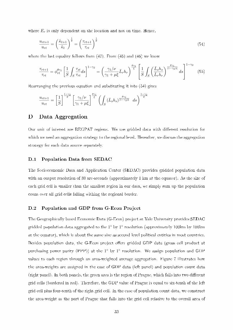
values to each region through an area-weighted average aggregation. Figure 7 illustrates how

the area-weights are assigned in the case of GDP data (left panel) and population count data

(right panel). In both panels, the green area is the region of Prague, which falls into two dierent

grid cells (bordered in red). Therefore, the GDP value of Prague is equal to six-tenth of the left

grid cell plus four-tenth of the right grid cell. In the case of population count data, we construct

the area-weight as the part of Prague that falls into the grid cell relative to the overall area of

33

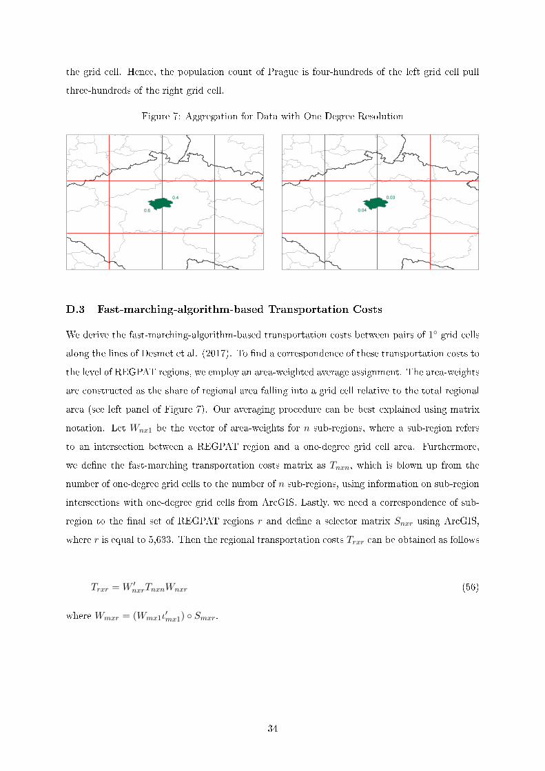
the grid cell. Hence, the population count of Prague is four-hundreds of the left grid cell pull

three-hundreds of the right grid cell.

Figure 7: Aggregation for Data with One Degree Resolution

0.6

0.4

0.04

0.03

D.3 Fast-marching-algorithm-based Transportation Costs

We derive the fast-marching-algorithm-based transportation costs between pairs of 1 grid cells

along the lines of Desmet et al. (2017). To nd a correspondence of these transportation costs to

the level of REGPAT regions, we employ an area-weighted average assignment. The area-weights

are constructed as the share of regional area falling into a grid cell relative to the total regional

area (see left panel of Figure 7). Our averaging procedure can be best explained using matrix

notation. Let Wnx1 be the vector of area-weights for n sub-regions, where a sub-region refers

to an intersection between a REGPAT region and a one-degree grid cell area. Furthermore,

we dene the fast-marching transportation costs matrix as Tnxn, which is blown up from the

number of one-degree grid cells to the number of n sub-regions, using information on sub-region

intersections with one-degree grid cells from ArcGIS. Lastly, we need a correspondence of sub-

region to the nal set of REGPAT regions r and dene a selector matrix Snxr using ArcGIS,

where r is equal to 5,633. Then the regional transportation costs Trxr can be obtained as follows

Trxr = W ′nxrTnxnWnxr (56)

where Wmxr = (Wmx1ι′mx1) Smxr.

34