The Discrete Cosine Transform (DCT) - Michigan … Discrete Cosine Transform (DCT): Theory and Application1 Syed Ali Khayam Department of Electrical & Computer Engineering Michigan

The Discrete Cosine Transform

(DCT):

Theory and Application1

Syed Ali Khayam

Department of Electrical & Computer Engineering

Michigan State University

March 10th 2003

1 This document is intended to be tutorial in nature. No prior knowledge of image processing concepts is assumed. Interested readers should follow the references for advanced material on DCT.

ECE 802 – 602: Information Theory and Coding Seminar 1 – The Discrete Cosine Transform: Theory and Application

1

1. Introduction

Transform coding constitutes an integral component of contemporary image/video processing

applications. Transform coding relies on the premise that pixels in an image exhibit a certain

level of correlation with their neighboring pixels. Similarly in a video transmission system,

adjacent pixels in consecutive frames2 show very high correlation. Consequently, these

correlations can be exploited to predict the value of a pixel from its respective neighbors. A

transformation is, therefore, defined to map this spatial (correlated) data into transformed

(uncorrelated) coefficients. Clearly, the transformation should utilize the fact that the information

content of an individual pixel is relatively small i.e., to a large extent visual contribution of a

pixel can be predicted using its neighbors.

A typical image/video transmission system is outlined in Figure 1. The objective of the source

encoder is to exploit the redundancies in image data to provide compression. In other words, the

source encoder reduces the entropy, which in our case means decrease in the average number of

bits required to represent the image. On the contrary, the channel encoder adds redundancy to the

output of the source encoder in order to enhance the reliability of the transmission. Clearly, both

these high-level blocks have contradictory objectives and their interplay is an active research

area ([1], [2], [3], [4], [5], [6], [7], [8]). However, discussion on joint source channel coding is

out of the scope of this document and this document mainly focuses on the transformation block

in the source encoder. Nevertheless, pertinent details about other blocks will be provided as

required.

2 Frames usually consist of a representation of the original data to be transmitted, together with other bits which may be used for error detection and control [9]. In simplistic terms, frames can be referred to as consecutive images in a video transmission.


2

Transformation Quantizer Entropy

Encoder

Source Encoder

Channel

Encoder

Inverse

Transformation

Inverse

Quantizer

Entropy

Decoder

Source Decoder

Channel

Decoder

Transmission

Channel

Original

Image

Reconstructed

Image

Figure 1. Components of a typical image/video transmission system [10].

As mentioned previously, each sub-block in the source encoder exploits some redundancy in the

image data in order to achieve better compression. The transformation sub-block decorrelates the

image data thereby reducing (and in some cases eliminating) interpixel redundancy3 [11]. The

two images shown in Figure 2 (a) and (b) have similar histograms (see Figure 2 (c) and (d)).

Figure 2 (f) and (g) show the normalized autocorrelation among pixels in one line of the

respective images. Figure 2 (f) shows that the neighboring pixels of Figure 2 (b) periodically

exhibit very high autocorrelation. This is easily explained by the periodic repetition of the

vertical white bars in Figure 2(b). This example will be will be employed in the following

sections to illustrate the decorrelation properties of transform coding. Here, it is noteworthy that

transformation is a lossless operation, therefore, the inverse transformation renders a perfect

reconstruction of the original image.

3 The term interpixel redundancy encompasses a broad class of redundancies, namely spatial redundancy, geometric redundancy and interframe redundancy [10]. However throughout this document (with the exception of Section 3.2), interpixel redundancy and spatial redundancy are used synonymously.


3

(a) (b)

0 50 100 150 200 250

0

0.5

1

1.5

2

2.5

x 104

0 50 100 150 200 250

0

0.5

1

1.5

2

x 104

(c) (d)

0 50 100 150 200 250 300 3500

0.1

0.2

0.3

0.4

0.5

0.6

0.7

0.8

0.9

1

0 50 100 150 200 250 300 350

0

0.1

0.2

0.3

0.4

0.5

0.6

0.7

0.8

0.9

1

(e) (f)

Figure 2. (a) First image, (b) second image, (c) histogram of first image, (d) histogram of second image, (e) normalized autocorrelation of one line of first image, (f) normalized

autocorrelation of one line of second image.

The quantizer sub-block utilizes the fact that the human eye is unable to perceive some visual

information in an image. Such information is deemed redundant and can be discarded without

introducing noticeable visual artifacts. Such redundancy is referred to as psychovisual

redundancy [10]. This idea can be extended to low bitrate receivers which, due to their stringent

bandwidth requirements, might sacrifice visual quality in order to achieve bandwidth efficiency.


4

This concept is the basis for rate distortion theory, that is, receivers might tolerate some visual

distortion in exchange for bandwidth conservation.

Lastly, the entropy encoder employs its knowledge of the transformation and quantization

processes to reduce the number of bits required to represent each symbol at the quantizer output.

Further discussion on the quantizer and entropy encoding sub-blocks is out of the scope of this

document.

In the last decade, Discrete Cosine Transform (DCT) has emerged as the de-facto image

transformation in most visual systems. DCT has been widely deployed by modern video coding

standards, for example, MPEG, JVT etc. This document introduces the DCT, elaborates its

important attributes and analyzes its performance using information theoretic measures.

2. The Discrete Cosine Transform

Like other transforms, the Discrete Cosine Transform (DCT) attempts to decorrelate the image

data. After decorrelation each transform coefficient can be encoded independently without losing

compression efficiency. This section describes the DCT and some of its important properties.

2.1. The One-Dimensional DCT

The most common DCT definition of a 1-D sequence of length N is

( ) ( ) ( )∑−

=⎥⎦⎤

⎢⎣⎡ +=

1

02

)12(cos

N

xN

uxxfuuC

πα , (1)

for 0,1,2, , 1u N= −… . Similarly, the inverse transformation is defined as


5

( ) ( ) ( )∑−

=⎥⎦⎤

⎢⎣⎡ +=

1

02

)12(cos

N

uN

uxuCuxf

πα , (2)

for 0,1,2, , 1x N= −… . In both equations (1) and (2) α(u) is defined as

1 0( )

2 0.

for uNu

for uN

α

⎧⎪⎪ =⎪⎪⎪⎪= ⎨⎪⎪ ≠⎪⎪⎪⎪⎩

(3)

It is clear from (1) that for 0u = , ( ) ( )∑−

=

==1

0

10

N

x

xfN

uC . Thus, the first transform coefficient is

the average value of the sample sequence. In literature, this value is referred to as the DC

Coefficient. All other transform coefficients are called the AC Coefficients4.

To fix ideas, ignore the ( )f x and ( )uα component in (1). The plot of ∑−

=⎥⎦⎤

⎢⎣⎡ +1

02

)12(cos

N

xN

uxπ for

8N = and varying values of u is shown in Figure 3. In accordance with our previous

observation, the first the top-left waveform ( 0u = ) renders a constant (DC) value, whereas, all

other waveforms ( 1,2, ,7u = … ) give waveforms at progressively increasing frequencies [13].

These waveforms are called the cosine basis function. Note that these basis functions are

orthogonal. Hence, multiplication of any waveform in Figure 3 with another waveform followed

by a summation over all sample points yields a zero (scalar) value, whereas multiplication of any

waveform in Figure 3 with itself followed by a summation yields a constant (scalar) value.

Orthogonal waveforms are independent, that is, none of the basis functions can be represented as

a combination of other basis functions [14].

4 These names come from the historical use of DCT for analyzing electric circuits with direct- and alternating-currents.


6

1 2 3 4 5 6 7 80

0.5

1u=0

1 2 3 4 5 6 7 8-1

0

1u=1

1 2 3 4 5 6 7 8-1

0

1u=2

1 2 3 4 5 6 7 8-1

0

1u=3

1 2 3 4 5 6 7 8-1

0

1u=4

1 2 3 4 5 6 7 8-1

0

1u=5

1 2 3 4 5 6 7 8-1

0

1u=6

1 2 3 4 5 6 7 8-1

0

1u=7

Figure 3. One dimensional cosine basis function (N=8).

If the input sequence has more than N sample points then it can be divided into sub-sequences

of length N and DCT can be applied to these chunks independently. Here, a very important

point to note is that in each such computation the values of the basis function points will not

change. Only the values of ( )f x will change in each sub-sequence. This is a very important

property, since it shows that the basis functions can be pre-computed offline and then multiplied

with the sub-sequences. This reduces the number of mathematical operations (i.e.,

multiplications and additions) thereby rendering computation efficiency.

2.2. The Two-Dimensional DCT

The objective of this document is to study the efficacy of DCT on images. This necessitates the

extension of ideas presented in the last section to a two-dimensional space. The 2-D DCT is a

direct extension of the 1-D case and is given by


7

( ) ( ) ( ) ( )∑∑−

=

−

=⎥⎦⎤

⎢⎣⎡ +

⎥⎦⎤

⎢⎣⎡ +=

1

0

1

02

)12(cos

2

)12(cos,,

N

x

N

yN

vy

N

uxyxfvuvuC

ππαα , (4)

for , 0,1,2, , 1u v N= −… and ( )uα and ( )vα are defined in (3). The inverse transform is

defined as

( ) ( ) ( ) ( )∑∑−

=

−

=⎥⎦⎤

⎢⎣⎡ +

⎥⎦⎤

⎢⎣⎡ +=

1

0

1

02

)12(cos

2

)12(cos,,

N

u

N

vN

vy

N

uxvuCvuyxf

ππαα , (5)

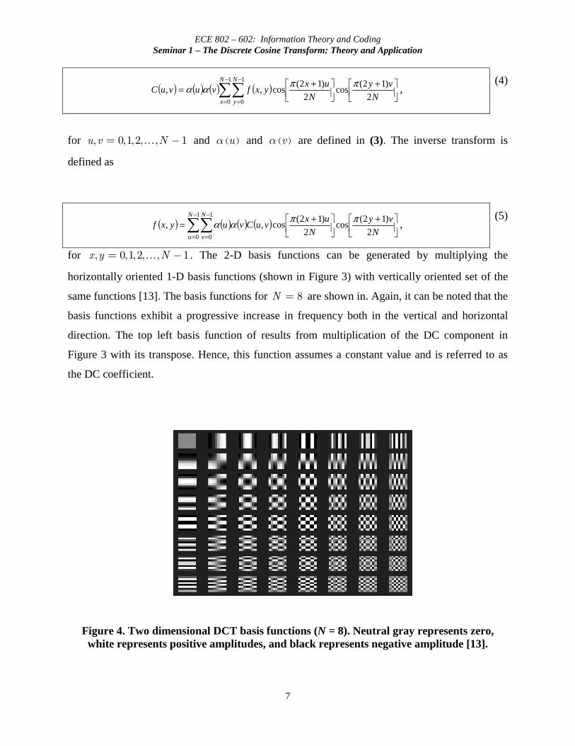
for , 0,1,2, , 1x y N= −… . The 2-D basis functions can be generated by multiplying the

horizontally oriented 1-D basis functions (shown in Figure 3) with vertically oriented set of the

same functions [13]. The basis functions for 8N = are shown in. Again, it can be noted that the

basis functions exhibit a progressive increase in frequency both in the vertical and horizontal

direction. The top left basis function of results from multiplication of the DC component in

Figure 3 with its transpose. Hence, this function assumes a constant value and is referred to as

the DC coefficient.

Figure 4. Two dimensional DCT basis functions (N = 8). Neutral gray represents zero,

white represents positive amplitudes, and black represents negative amplitude [13].


8

2.3. Properties of DCT

Discussions in the preceding sections have developed a mathematical foundation for DCT.

However, the intuitive insight into its image processing application has not been presented. This

section outlines (with examples) some properties of the DCT which are of particular value to

image processing applications.

2.3.1. Decorrelation

As discussed previously, the principle advantage of image transformation is the removal of

redundancy between neighboring pixels. This leads to uncorrelated transform coefficients which

can be encoded independently. Let us consider our example from Figure 2 to outline the

decorrelation characteristics of the 2-D DCT. The normalized autocorrelation of the images

before and after DCT is shown in Figure 5. Clearly, the amplitude of the autocorrelation after the

DCT operation is very small at all lags. Hence, it can be inferred that DCT exhibits excellent

decorrelation properties.

0 50 100 150 200 250 300 3500

0.1

0.2

0.3

0.4

0.5

0.6

0.7

0.8

0.9

1

0 50 100 150 200 250 300 350

-0.4

-0.2

0

0.2

0.4

0.6

0.8

1

(a)

0 50 100 150 200 250 300 3500

0.1

0.2

0.3

0.4

0.5

0.6

0.7

0.8

0.9

1

0 50 100 150 200 250 300 350

-0.4

-0.2

0

0.2

0.4

0.6

0.8

1

(b)

Figure 5. (a) Normalized autocorrelation of uncorrelated image before and after DCT; (b) Normalized autocorrelation of correlated image before and after DCT.


9

2.3.2. Energy Compaction

Efficacy of a transformation scheme can be directly gauged by its ability to pack input data into

as few coefficients as possible. This allows the quantizer to discard coefficients with relatively

small amplitudes without introducing visual distortion in the reconstructed image. DCT exhibits

excellent energy compaction for highly correlated images.

Let us again consider the two example images of Figure 2(a) and (b). In addition to their

respective correlation properties discussed in preceding sections, the uncorrelated image has

more sharp intensity variations than the correlated image. Therefore, the former has more high

frequency content than the latter. Figure 6 shows the DCT of both the images. Clearly, the

uncorrelated image has its energy spread out, whereas the energy of the correlated image is

packed into the low frequency region (i.e., top left region).

(a)

(b)

Figure 6. (a) Uncorrelated image and its DCT; (b) Correlated image and its DCT.


10

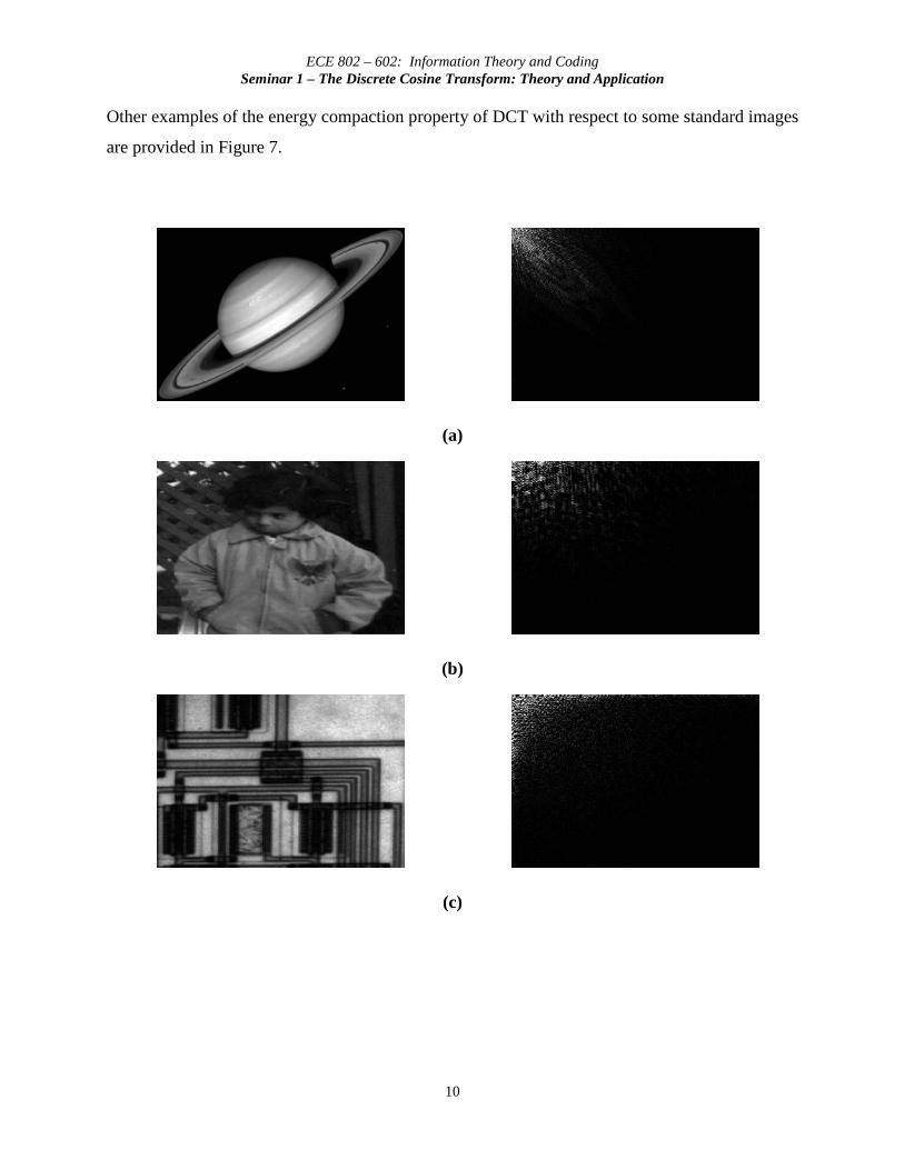
Other examples of the energy compaction property of DCT with respect to some standard images

are provided in Figure 7.

(a)

(b)

(c)


11

(d)

(e)

(f)

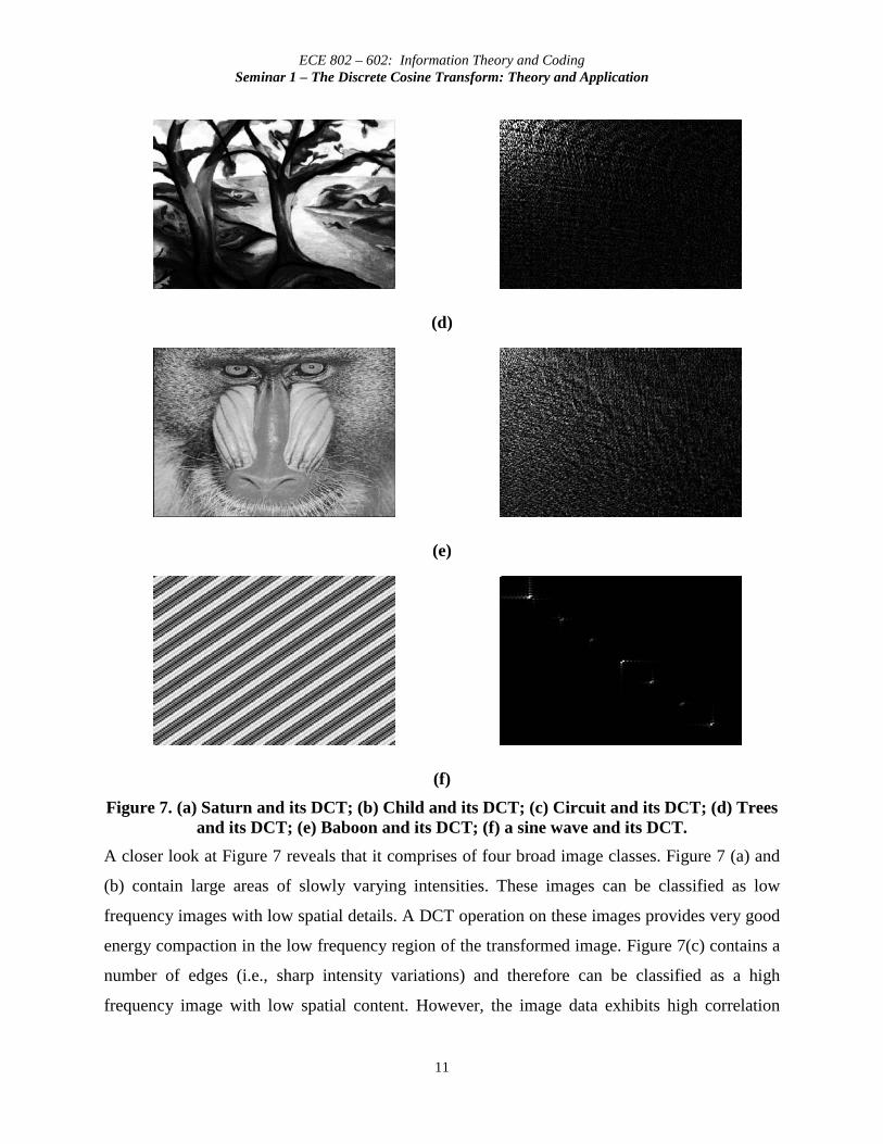
Figure 7. (a) Saturn and its DCT; (b) Child and its DCT; (c) Circuit and its DCT; (d) Trees and its DCT; (e) Baboon and its DCT; (f) a sine wave and its DCT.

A closer look at Figure 7 reveals that it comprises of four broad image classes. Figure 7 (a) and

(b) contain large areas of slowly varying intensities. These images can be classified as low

frequency images with low spatial details. A DCT operation on these images provides very good

energy compaction in the low frequency region of the transformed image. Figure 7(c) contains a

number of edges (i.e., sharp intensity variations) and therefore can be classified as a high

frequency image with low spatial content. However, the image data exhibits high correlation


12

which is exploited by the DCT algorithm to provide good energy compaction. Figure 7 (d) and

(e) are images with progressively high frequency and spatial content. Consequently, the

transform coefficients are spread over low and high frequencies. Figure 7(e) shows periodicity

therefore the DCT contains impulses with amplitudes proportional to the weight of a particular

frequency in the original waveform. The other (relatively insignificant) harmonics of the sine

wave can also be observed by closer examination of its DCT image.

Hence, from the preceding discussion it can be inferred that DCT renders excellent energy

compaction for correlated images. Studies have shown that the energy compaction performance

of DCT approaches optimality as image correlation approaches one i.e., DCT provides (almost)

optimal decorrelation for such images [15].

2.3.3. Separability

The DCT transform equation (4) can be expressed as,

( ) ( ) ( ) ( )∑ ∑−

=

−

=⎥⎦⎤

⎢⎣⎡ +

⎥⎦⎤

⎢⎣⎡ +=

1

0

1

02

)12(cos,

2

)12(cos,

N

x

N

yN

vyyxf

N

uxvuvuC

ππαα , (6)

for , 0,1,2, , 1u v N= −… .

This property, known as separability, has the principle advantage that C(u, v) can be computed in

two steps by successive 1-D operations on rows and columns of an image. This idea is

graphically illustrated in Figure 8. The arguments presented can be identically applied for the

inverse DCT computation (5).

Figure 8. Computation of 2-D DCT using separability property.

y

x

f(x, y)

C(x, v)

C(u, v) Row transform Column transform


13

2.3.4. Symmetry

Another look at the row and column operations in Equation 6 reveals that these operations are

functionally identical. Such a transformation is called a symmetric transformation. A separable

and symmetric transform can be expressed in the form [10]

AfAT = , (7)

where A is an N N× symmetric transformation matrix with entries ( ),a i j given by

( ) ( )∑−

=⎥⎦⎤

⎢⎣⎡ +=

1

02

)12(cos,

N

jN

ijjjia

πα ,

and f is the N N× image matrix.

This is an extremely useful property since it implies that the transformation matrix5 can be pre-

computed offline and then applied to the image thereby providing orders of magnitude

improvement in computation efficiency.

2.3.5. Orthogonality

In order to extend ideas presented in the preceding section, let us denote the inverse

transformation of (7) as

11 −−= TAAf .

As discussed previously, DCT basis functions are orthogonal (See Section 2.1). Thus, the inverse

transformation matrix of A is equal to its transpose i.e. A-1= AT. Therefore, and in addition to its

5 In image processing jargon this matrix is referred to as the transformation kernel. In our scenario it comprises of the basis functions of Figure 4.


14

decorrelation characteristics, this property renders some reduction in the pre-computation

complexity.

2.4. A Faster DCT

The properties discussed in the last three sub-sections have laid the foundation for a faster DCT

computation algorithm. Generalized and architecture-specific fast DCT algorithms have been

studied extensively ([17], [18], [19], [20], [21], [22], [23], [24], [25],[26], [27], [28], [29], [30],

[31]). However, and in accordance with the readers’ engineering background, we only discuss

one algorithm that utilizes the Fast Fourier Transform (FFT) to compute the DCT and its inverse

[16]. This algorithm is presented for the 1-D DCT nevertheless it can be extended to the 2-D

case. Here, it is important to note that DCT is not the real part of the Discrete Fourier Transform

(DFT). This can be easily verified by inspecting the DCT and DFT transformation matrices.

The 1-D sequence ( )f x in (1) can be expressed as a sum of an even and an odd sequence

( ) ( ) ( )xfxfxf oe +=~

,

where ( ) ( ) ( )xfxfxfe

~

2 == , ( ) ( ) ( )112~

−−=+= xNfxfxfo , and 12

0 −⎟⎠⎞

⎜⎝⎛≤≤ N

x .

The summation term in (1) can be split to obtain


15

( ) ( ) ( ) ( )

( ) ( ) ( )

1 12 2

0 0

12 2

0 0

(4 1) (4 3)2 cos 2 1 cos2 2

(4 1) (4 3)cos cos2 2

N N

x x

N N

e ox x

x u x uC u u f x f xN N

x u x uu f x f xN N

π πα

π πα

⎛ ⎞ ⎛ ⎞⎟ ⎟⎜ ⎜− −⎟ ⎟⎜ ⎜⎟ ⎟⎜ ⎜⎝ ⎠ ⎝ ⎠

= =

⎛ ⎞ ⎛ ⎞⎟⎜ ⎜−⎟⎜ ⎜⎟⎜ ⎜⎝ ⎠ ⎝ ⎠

= =

⎧ ⎫⎪ ⎪⎪ ⎪⎪ ⎪⎡ ⎤ ⎡ ⎤+ +⎪ ⎪⎪ ⎪= ⎢ ⎥ + + ⎢ ⎥⎨ ⎬⎪ ⎪⎢ ⎥ ⎢ ⎥⎣ ⎦ ⎣ ⎦⎪ ⎪⎪ ⎪⎪ ⎪⎪ ⎪⎩ ⎭

⎡ ⎤ ⎡ ⎤+ += ⎢ ⎥ + ⎢ ⎥⎢ ⎥ ⎢ ⎥⎣ ⎦ ⎣ ⎦

∑ ∑

∑

( ) ( )

( ) ( ) ( ) ( ){ }

1

1 ~

01 ~ ~/2/2 2 /

20

(4 1)cos2

Re Re .

N

xN uj u N j ux N

NNx

n uu f xN

u e f x e u W DFT f xπ π

πα

α α

⎟−⎟⎟

−

=−

− −

=

⎧ ⎫⎪ ⎪⎪ ⎪⎪ ⎪⎪ ⎪⎪ ⎪⎨ ⎬⎪ ⎪⎪ ⎪⎪ ⎪⎪ ⎪⎪ ⎪⎩ ⎭⎡ ⎤+= ⎢ ⎥⎢ ⎥⎣ ⎦

⎡ ⎤ ⎡ ⎤⎢ ⎥ ⎢ ⎥= =⎢ ⎥ ⎢ ⎥⎣ ⎦⎣ ⎦

∑

∑

∑

For the inverse transformation, we can calculate ( ) )2(2~

xfxf = and the odd points can be

calculated by noting that ( ) ( )[ ]xNfxf −−=+ 1212~

for 12

0 −⎟⎠⎞

⎜⎝⎛≤≤ N

x .

2.5. DCT versus DFT/KLT

At this point it is important to mention the superiority of DCT over other image transforms.

More specifically, we compare DCT with two linear transforms: 1) The Karhunen-Loeve

Transform (KLT); 2) Discrete Fourier Transform (DFT).

The KLT is a linear transform where the basis functions are taken from the statistical properties

of the image data, and can thus be adaptive. It is optimal in the sense of energy compaction, i.e.,

it places as much energy as possible in as few coefficients as possible. However, the KLT

transformation kernel is generally not separable, and thus the full matrix multiplication must be

performed. In other words, KLT is data dependent and, therefore, without a fast (FFT-like) pre-

computation transform. Derivation of the respective basis for each image sub-block requires

unreasonable computational resources. Although, some fast KLT algorithms have been

suggested ([32], [33]), nevertheless the overall complexity of KLT is significantly higher than

the respective DCT and DFT algorithms.


16

In accordance with the readers’ background, familiarity with Discrete Fourier Transform (DFT)

has been assumed throughout this document. The DFT transformtion kernel is linear, separable

and symmetric. Hence, like DCT, it has fixed basis images and fast implementations are

possible. It also exhibits good decorrelation and energy compaction characterictics. However, the

DFT is a complex transform and therefore stipulates that both image magnitude and phase

information be encoded. In addition, studies have shown that DCT provides better energy

compaction than DFT for most natural images. Furthermore, the implicit periodicity of DFT

gives rise to boundary discontinuties that result in significant high-frequency content. After

quantization, Gibbs Phenomeneon causes the boundary points to take on erraneous values [11].

3. DCT Performance Evaluation: An Information

Theoretic Approach

In this section we investigate the performance of DCT using information theory measures.

3.1. Entropy Reduction

The decorrelation characteristics of DCT should render a decrease in the entropy (or self-

information) of an image. This will, in turn, decrease the number of bits required to represent the

image. Entropy is defined as

( ) ( )( )i

N

ii xpxpXH log)(

1∑

=

−= ,

where ( )ip x is the value of the probability mass function (pmf) at iX x= . Throughout the

following discussion, the pmf refers to the normalized histogram of an image.

The first column of Table 1 gives the entropy of the images listed in Figure 7. All following

columns tabulate the entropies of the respective DCT images with a certain number of


17

coefficients retained. More specifically, DCT (M%) means that after the DCT operation only the

first M percent of the total coefficients are retained. Consider for instance a 352x288 image,

DCT (25%) retains only 25% (352x288x0.25=25560) of the total (102240) coefficients.

It should be emphasized again that this decrease in entropy represents a reduction in the average

number of bits required for a particular image. The second column of Table 1 clearly shows that

the DCT operation reduces the entropy of all images. The reduction in entropy becomes more

profound as we decrease the number of retained coefficients (see Table 1 columns 3, 4, and 5).

This very interesting result implies that discarding some high frequency details can yield

significant dividend in reducing the overall entropy. It is noteworthy that the inherent lossless

nature of the transform encoder dictates that the coefficient discarding operation be implemented

in the quantizer.

Image Entropy original image

Entropy DCT (75%)

Entropy DCT (50%)

Entropy DCT (25%)

Saturn 4.1140 1.9144 0.7504 0.2181 Child 5.7599 1.7073 0.7348 0.2139 Circuit 6.9439 1.4961 0.6906 0.2120 Trees 5.7006 1.1445 0.6181 0.2081 Baboon 7.3461 0.9944 0.5859 0.2058 Sine 3.125 1.2096 0.6674 0.2125

Table 1. Entropy of images and their DCT.

A closer look at the Table 1 reveals that the entropy reduction for the Baboon image is very

drastic. The entropy of the original image ascertains that it has a lot of high frequency

component and spatial detail. Therefore, coding it in the spatial domain is very inefficient since

the gray levels are somewhat uniformly distributed across the image. However, the DCT

decorrelates the image data thereby stretching the histogram. This discussion also applies to the

other high frequency images, namely Circuit and Trees. The decrease in entropy is easily

explained by observing the histograms of the original and the DCT encoded images in Figure 9.

As a consequence of the decorrelation property, the original image data is transformed in a way

that the histogram is stretched and the amplitude of most transformed outcomes is very small.


18

0 50 100 150 200 250

0

2000

4000

6000

8000

10000

12000

0 0.1 0.2 0.3 0.4 0.5 0.6 0.7 0.8 0.9 1

0

2000

4000

6000

8000

10000

12000

(a)

0 50 100 150 200 250

0

200

400

600

800

1000

1200

1400

1600

0 0.1 0.2 0.3 0.4 0.5 0.6 0.7 0.8 0.9 1

0

1000

2000

3000

4000

5000

6000

(b)

0 50 100 150 200 250

0

200

400

600

800

1000

0 0.1 0.2 0.3 0.4 0.5 0.6 0.7 0.8 0.9 1

0

1000

2000

3000

4000

5000

6000

7000

(c)


19

0 50 100 150 200 250

0

500

1000

1500

2000

2500

0 0.1 0.2 0.3 0.4 0.5 0.6 0.7 0.8 0.9 1

0

500

1000

1500

2000

(d)

0 50 100 150 200 250

0

500

1000

1500

2000

2500

3000

0 0.1 0.2 0.3 0.4 0.5 0.6 0.7 0.8 0.9 1

0

500

1000

1500

2000

2500

3000

(e)

0 50 100 150 200 250

0

100

200

300

400

500

600

700

800

0 0.1 0.2 0.3 0.4 0.5 0.6 0.7 0.8 0.9 1

0

200

400

600

800

1000

1200

1400

1600

1800

(f)

Figure 9. (a) Histogram of Saturn and its DCT; (b) Histogram of Child and its DCT; (c) Histogram of Circuit and its DCT; (d) Histogram of Trees and its DCT; (e) Histogram of

Baboon and its DCT; (f) Histogram of a sine wave and its DCT.


20

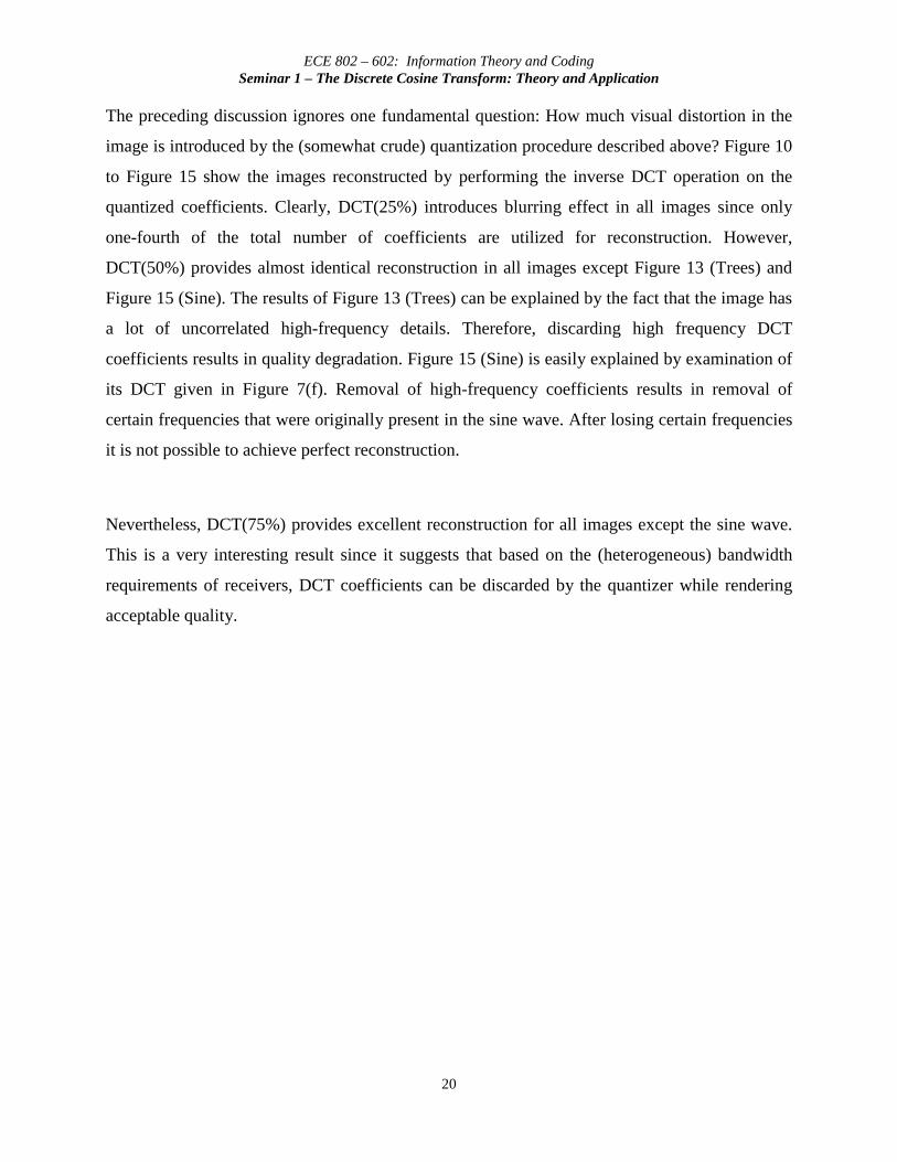
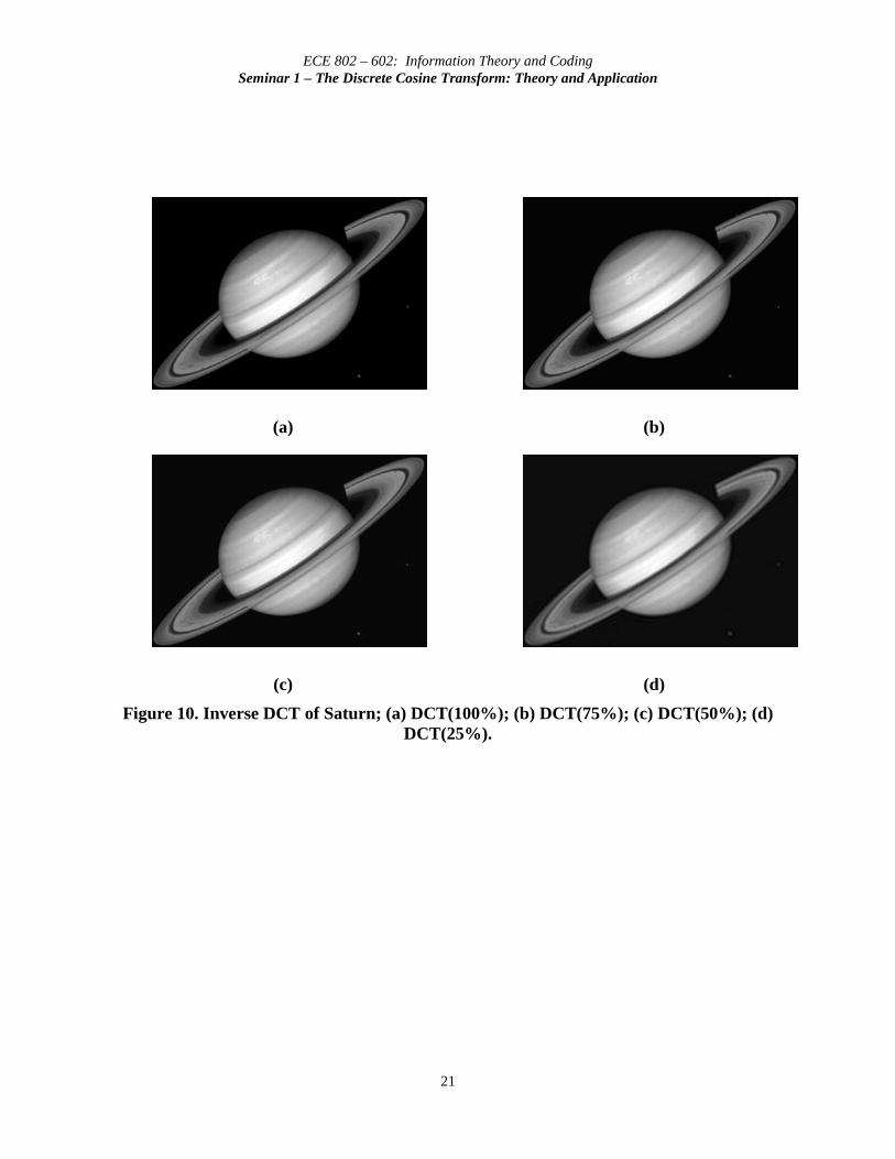
The preceding discussion ignores one fundamental question: How much visual distortion in the

image is introduced by the (somewhat crude) quantization procedure described above? Figure 10

to Figure 15 show the images reconstructed by performing the inverse DCT operation on the

quantized coefficients. Clearly, DCT(25%) introduces blurring effect in all images since only

one-fourth of the total number of coefficients are utilized for reconstruction. However,

DCT(50%) provides almost identical reconstruction in all images except Figure 13 (Trees) and

Figure 15 (Sine). The results of Figure 13 (Trees) can be explained by the fact that the image has

a lot of uncorrelated high-frequency details. Therefore, discarding high frequency DCT

coefficients results in quality degradation. Figure 15 (Sine) is easily explained by examination of

its DCT given in Figure 7(f). Removal of high-frequency coefficients results in removal of

certain frequencies that were originally present in the sine wave. After losing certain frequencies

it is not possible to achieve perfect reconstruction.

Nevertheless, DCT(75%) provides excellent reconstruction for all images except the sine wave.

This is a very interesting result since it suggests that based on the (heterogeneous) bandwidth

requirements of receivers, DCT coefficients can be discarded by the quantizer while rendering

acceptable quality.


21

(a) (b)

(c) (d)

Figure 10. Inverse DCT of Saturn; (a) DCT(100%); (b) DCT(75%); (c) DCT(50%); (d) DCT(25%).


22

(a) (b)

(c) (d)

Figure 11. Inverse DCT of Child; (a) DCT(100%); (b) DCT(75%); (c) DCT(50%);

(d) DCT(25%).


23

(a) (b)

(c) (d)

Figure 12. Inverse DCT of Circuit; (a) DCT(100%); (b) DCT(75%); (c) DCT(50%);

(d) DCT(25%).


24

(a) (b)

(c) (d)

Figure 13. Inverse DCT of Trees; (a) DCT(100%); (b) DCT(75%); (c) DCT(50%);

(d) DCT(25%).


25

(a) (b)

(c) (d)

Figure 14. Inverse DCT of Baboon; (a) DCT(100%); (b) DCT(75%); (c) DCT(50%);

(d) DCT(25%).


26

(a) (b)

(c) (d)

Figure 15. Inverse DCT of sine wave; (a) DCT(100%); (b) DCT(75%); (c) DCT(50%);

(d) DCT(25%).

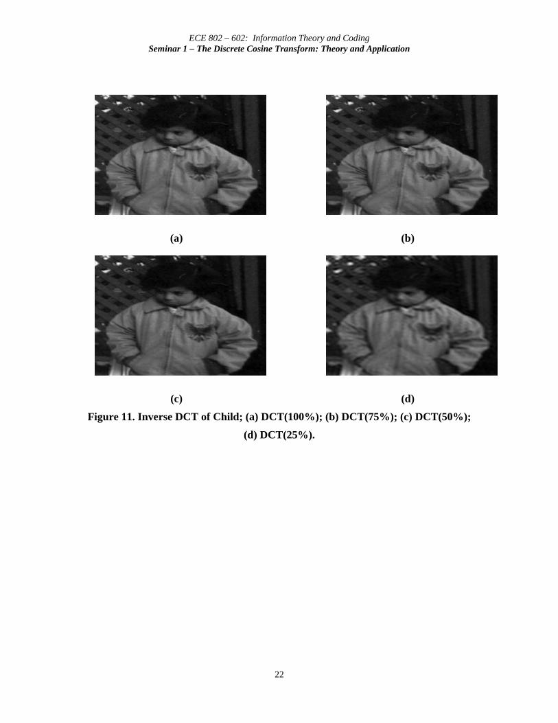
3.2. Mutual-Information

A video transmission comprises of a sequence of images (referred to as frames) that are

transmitted in a specified order. Generally, the change of information between consecutive video

frames is quite low. Hence, pixel values in one frame can be used to predict the adjacent pixels

of the next frame. This phenomenon is referred to temporal correlation. Such temporal

redundancy can be removed to provide better compression. However, it should be obvious that if

the two respective frames represent a scene change then the mutual information is reduced. This

is clearly shown in Figure 16. The first two frames exhibit high temporal correlation. However,

frame-2 and frame-3 represent a change in scene, therefore the information overlap between

these frames is relatively smaller.


27

Frame-1 Frame-2 Frame-3

Figure 16. Three consecutive frame of a video sequence.

We utilize the Mutual Information Measure to quantify the temporal correlation between frames

of a video sequence. Mutual information of two video frames can, therefore, be characterized as

the amount of redundancy (correlation) between the two frames. Mutual Information is given by

( ) ( ) ( )( ) ( ),

; , logx y

p x yI X Y p x y

p x p y

⎛ ⎞⎟⎜ ⎟= ⎜ ⎟⎜ ⎟⎟⎜⎝ ⎠∑∑ ,

where ( ),p x y is the joint probability mass function (pmf) of random variables X and Y (i.e.,

frame-X and frame-Y in our case), ( )p x and ( )p y represent the marginal pmf of X and Y

respectively.

Let us consider the mutual information of the video frames shown in Figure 16. Let ( ),p x y be

defined by coupling the values of adjacent pixels in any two consecutive frames. The allowed

range of values for ( ),p x y is (0, 0), (0, 1), (0, 2), ……, (255, 255). Hence, the total number of

outcomes is (255)2. In addition, let ( )p x and ( )p y be the normalized histograms of frame-X

and frame-Y respectively. The mutual information is as follows:

Mutual Information between frame-1 and frame-2:

Mutual Information between frame-2 and frame-3:

1.9336

0.2785


28

Since, there exists high temporal correlation between the first two frames, therefore, their mutual

information is quite high. However, frame-2 and frame-3 represent a change in video scene,

hence, the mutual information of the two images is relatively smaller.

These results outline a very interesting phenomenon, and that is, frames in a video sequence

exhibit high temporal correlation. Such temporal redundancies can be exploited by the source

encoder to improve coding efficiency. In other words, adjacent pixels from past and future video

frames can be used to predict the pixel values in a particular frame. This temporal correlation is

employed by most contemporary video processing systems. Further discussion on this topic is

out of the scope of this document.

4. Conclusions and Future Directions

The results presented in this document show that the DCT exploits interpixel redundancies to

render excellent decorrelation for most natural images. Thus, all (uncorrelated) transform

coefficients can be encoded independently without compromising coding efficiency. In addition,

the DCT packs energy in the low frequency regions. Therefore, some of the high frequency

content can be discarded without significant quality degradation. Such a (course) quantization

scheme causes further reduction in the entropy (or average number of bits per pixel). Lastly, it is

concluded that successive frames in a video transmission exhibit high temporal correlation

(mutual information). This correlation can be employed to improve coding efficiency.

The aforementioned attributes of the DCT have led to its widespread deployment in virtually

every image/video processing standard of the last decade, for example, JPEG (classical), MPEG-

1, MPEG-2, MPEG-4, MPEG-4 FGS, H.261, H.263 and JVT (H.26L). Nevertheless, the DCT

still offers new research directions that are being explored in the current and upcoming

image/video coding standards ([35], [36], [37], [38], [39], [40]).


29

5. References

[1] K. Ramchandran, A. Ortega, K. Metin Uz, and M. Vetterli, “Multiresolution broadcast for

digital HDTV using joint source/channel coding.” IEEE Journal on Selected Areas in

Communications, 11(1):6−23, January 1993.

[2] M. W. Garrett and M. Vetterli, “Joint Source/Channel Coding of Statistically Multiplexed

Real Time Services on Packet Networks,” IEEE/ACM Transactions on Networking, 1993.

[3] S. McCanne and M. Vetterli, “Joint source/channel coding for multicast packet video,”

International Conference on Image Processing (Vol. 1)-Volume 1, October 1995,

Washington D.C.

[4] K. Sayood and J. C. Borkenhagen, “Use of residual redundancy in the design of joint

source/channel coders,” IEEE Transactions on Communications, 39(6):838-846, June

1991.

[5] J. Modestino, D.G. Daut, and A. Vickers, “Combined source channel coding of images

using the block cosine transform,” IEEE Transactions on Communications, vol. 29,

pp.1261-1274, September 1981.

[6] T. Cover, “Broadcast Channels,” IEEE Transactions on Information Theory, vol. 18, pp. 2-

14, January 1972.

[7] Q. Zhang, Z. Ji, W. Zhu, J. Lu, and Y.-Q. Zhang, “Joint power control and source-channel

coding for video communication over wireless,” IEEE VTC’01, October 2001, New Jersey.

[8] Q. Zhang, W. Zhu, Zu Ji, and Y. Zhang, “A Power-Optimized Joint Source Channel

Coding for Scalable Video Streaming over Wireless Channel," IEEE ISCAS’01, May,

2001, Sydney, Australia.

[9] T1.523-2001, American National Standard: Telecom Glossary 2000.

[10] Hayder Radha, “Lecture Notes: ECE 802 - Information Theory and Coding,” January

2003.

[11] R. C. Gonzalez and P. Wintz, “Digital Image Processing,” Reading. MA: Addison-Wesley,

1977.

[12] N. Ahmed, T. Natarajan, and K. R. Rao, “Discrete cosine transform,” IEEE Transactions

on Computers, vol. C-32, pp. 90-93, Jan. 1974.


30

[13] W. B. Pennebaker and J. L. Mitchell, “JPEG – Still Image Data Compression Standard,”

Newyork: International Thomsan Publishing, 1993.

[14] G. Strang, “The Discrete Cosine Transform,” SIAM Review, Volume 41, Number 1, pp.

135-147, 1999.

[15] R. J. Clark, “Transform Coding of Images,” New York: Academic Press, 1985.

[16] A. K. Jain, “Fundamentals of Digital Image Processing,” New Jersey: Prentice Hall Inc.,

1989.

[17] A. C. Hung and TH-Y Meng, “A Comparison of fast DCT algorithms,” Multimedia

Systems, No. 5 Vol. 2, Dec 1994.

[18] G. Aggarwal and D. D. Gajski, “Exploring DCT Implementations,” UC Irvine, Technical

Report ICS-TR-98-10, March 1998.

[19] J. F. Blinn, “What's the Deal with the DCT,” IEEE Computer Graphics and Applications,

July 1993, pp.78-83.

[20] C. T. Chiu and K. J. R. Liu, “Real-Time Parallel and Fully Pipelined 2-D DCT Lattice

Structures with Application to HDTV Systems,” IEEE Trans. on Circuits and Systems for

Video Technology, vol. 2 pp. 25-37, March 1992.

[21] Haque, “A Two-Dimensional Fast Cosine Transform,” IEEE Transactions on Acoustics,

Speech and Signal Processing, vol. ASSP-33 pp. 1532-1539, December 1985.

[22] M. Vetterli, “Fast 2-D Discrete Cosine Transform,” ICASSP '85, p. 1538.

[23] F. A. Kamangar and K.R. Rao, “Fast Algorithms for the 2-D Discrete Cosine Transform,”

IEEE Transactions on Computers, v C-31 p. 899.

[24] E. N. Linzer and E. Feig, “New Scaled DCT Algorithms for Fused Multiply/Add

Architectures,” ICASSP '91, p. 2201.

[25] C. Loeffler, A. Ligtenberg, and G. Moschytz, “Practical Fast 1-D DCT Algorithms with 11

Multiplications,” ICASSP '89, p. 988.

[26] M. Vetterli, P. Duhamel, and C. Guillemot, “Trade-offs in the Computation of Mono- and

Multi-dimensional DCTs,” ICASSP '89, p. 999.

[27] P. Duhamel, C. Guillemot, and J. C. Carlach, “A DCT Chip based on a new Structured and

Computationally Efficient DCT Algorithm,” ICCAS '90, p. 77.

[28] N. I. Cho and S.U. Lee, “Fast Algorithm and Implementation of 2-D DCT,” IEEE

Transactions On Circuits and Systems, vol. 38 p. 297, March 1991.


31

[29] N. I. Cho, I. D. Yun, and S. U. Lee, “A Fast Algorithm for 2-D DCT,” ICASSP '91, p.

2197-2220.

[30] L. McMillan and L. Westover, “A Forward-Mapping Realization of the Inverse DCT,”

DCC '92, p. 219.

[31] P. Duhamel and C. Guillemot, “Polynomial Transform Computation of the 2-D DCT,”

ICASSP '90, p. 1515.

[32] J. E. Castrillon-Candas and K. Amaratunga, “Fast Estimation of Karhunen-Loeve Eigen

Function usin Wavelets,” Submitted to IEEE Transactions on Signal Processing, 2001.

[33] A. Jain, “A Fast Karhunen-loeve Transform for Digital Restoration of Images Degraded by

White and Colored Noise,” IEEE Transactions on Computers, vol. 26, number 6, June

1977.

[34] R. W. Yeung, “A First Course in Information Theory,” New York: Kluwer

Academic/Plenum Publishers, 2002.

[35] D. Marpe, G. Blättermann, and T. Wiegand, “An Overview of the Draft H.26L Video

Compression Standard,” IEEE Transactions on Circuits and Systems for Video

Technology, 2003.

[36] T. Stockhammer, T. Wiegand, and S. Wenger, “Optimized Transmission of H.26L/JVT

Coded Video Over Packet-Lossy Networks,” ICIP 2002.

[37] Special Tutorial issue on the MPEG-4 standard, Signal Processing: Image

Communication, 15(4−5), 2000 (Elsevier).

[38] S. Liu and A. C. Bovik, “Efficient DCT-domain Blind Measurement and Reduction of

Blocking Artifacts,” IEEE Transactions on Circuits and Systems for Video Technology,

April 2001.

[39] H. Radha, M. van der Schaar, Y. Chen, "The MPEG-4 Fine-Grained Scalable Video

Coding Method for Multimedia Streaming over IP," IEEE Transactions on Multimedia,

March, 2001.

[40] M. van der Schaar, Y. Chen, and H. Radha, “Embedded DCT and Wavelet Methods for

Scalable Video: Analysis and Comparison,” Visual Communications and Image

Processing, January 2000.

The Discrete Cosine Transform (DCT) - Michigan … Discrete Cosine Transform (DCT): Theory and Application1 Syed Ali Khayam Department of Electrical & Computer Engineering Michigan

Documents