The Decoupling of Linear Dynamical Systemsdigitalassets.lib.berkeley.edu/etd/ucb/text/Kawano... ·  · 2013-08-16The Decoupling of Linear Dynamical Systems by ... cedure that depends

The Decoupling of Linear Dynamical Systems

by

Daniel Takashi Kawano

A dissertation submitted in partial satisfaction of the

requirements for the degree of

Doctor of Philosophy

in

Engineering − Mechanical Engineering

in the

Graduate Division

of the

University of California, Berkeley

Committee in charge:

Professor Fai Ma, ChairProfessor Benson H. TongueProfessor Oliver M. O’Reilly

Professor John Strain

Spring 2011

The Decoupling of Linear Dynamical Systems

Copyright © 2011

by

Daniel Takashi Kawano

Abstract

The Decoupling of Linear Dynamical Systems

by

Daniel Takashi Kawano

Doctor of Philosophy in Engineering − Mechanical Engineering

University of California, Berkeley

Professor Fai Ma, Chair

Decoupling a second-order linear dynamical system requires that one develop a trans-formation that simultaneously diagonalizes the coefficient matrices that define the systemin terms of its distribution of inertia and viscoelasticity. A traditional approach to decou-pling a viscously damped system uses the eigenvectors of the corresponding undampedsystem to diagonalize the mass, damping, and stiffness matrices through a real congruencetransformation in the configuration space, a process known as classical modal analysis.However, it is well known that classical modal analysis fails to decouple a linear dynamicalsystem if its damping matrix does not satisfy a commutativity relationship involving thesystem matrices. Such a system is said to be non-classically damped. We demonstrate thatit is possible to decouple any non-classically damped system in the configuration and statespaces through generally time-dependent transformations constructed using spectral dataobtained from the solution of a quadratic eigenvalue problem.

When a non-classically damped system has complex but non-defective eigenvalues, theeffect of non-classical damping is that it introduces constant phase shifts among the com-ponents of the system’s free response. Decoupling of free vibration in the configurationspace is achieved through a real, linear, time-shifting transformation that eliminates thesephase differences, yielding classical modes of vibration. This decoupling transformation,referred to as phase synchronization, preserves both the eigenvalues and their multiplicities.When cast in a state space form, the transformation between the coupled and decoupledsystems is real, linear, but time-invariant. Through the concept of real quadratic conjuga-tion, we illustrate that there is no fundamental difference in the representation of the freeresponse of a system with complex eigenvalues and one with real eigenvalues, and thus sys-tems with non-defective real eigenvalues can also be decoupled by phase synchronization.When phase synchronization is extended to forced systems, the decoupling transformationin both the configuration and state spaces is nonlinear and depends continuously on theapplied excitation.

1

If a non-classically damped system is defective, it may only be partially decoupledif one insists on preserving the geometric multiplicities of the defective eigenvalues. Wepresent the first systematic effort to decouple defective systems in free or forced vibrationby not demanding invariance of the geometric multiplicities. In the course of this devel-opment, the notion of critical damping in multi-degree-of-freedom systems is clarified andexpanded. It is shown that the decoupling of defective systems is a rather delicate pro-cedure that depends on the multiplicities of the system eigenvalues. A generalized statespace-based decoupling transformation is developed that relates the response of any non-classically damped system to that of its decoupled form. In principle, one could extractfrom the state space a decoupling transformation in the configuration space, but it generallydoes not have an explicit form. The decoupling transformation in both the configurationand state spaces is real and time-dependent. Several numerical examples are provided toillustrate the theoretical developments.

2

Contents

List of Select Symbols iii

Acknowledgments v

1 Introduction 11.1 Classical modal analysis . . . . . . . . . . . . . . . . . . . . . . . . . . . . . . 21.2 Complex modal analysis . . . . . . . . . . . . . . . . . . . . . . . . . . . . . . 31.3 Approximate methods for non-classically damped systems . . . . . . . . . . 31.4 Exact methods for non-classically damped systems . . . . . . . . . . . . . . . 41.5 Goals and motivation for exact decoupling . . . . . . . . . . . . . . . . . . . 5

2 Decoupling of Non-Defective Systems in Free Motion 62.1 The quadratic eigenvalue problem . . . . . . . . . . . . . . . . . . . . . . . . 62.2 Complex eigenvalues . . . . . . . . . . . . . . . . . . . . . . . . . . . . . . . . 7

2.2.1 Underdamped modes of real vibration . . . . . . . . . . . . . . . . . . 72.2.2 The mechanics of phase synchronization . . . . . . . . . . . . . . . . 82.2.3 A configuration space representation of decoupling . . . . . . . . . . 102.2.4 A state space representation of decoupling . . . . . . . . . . . . . . . 10

2.3 Real eigenvalues . . . . . . . . . . . . . . . . . . . . . . . . . . . . . . . . . . 122.3.1 The concept of real quadratic conjugation . . . . . . . . . . . . . . . 132.3.2 Pure exponential decay as imaginary vibration . . . . . . . . . . . . . 142.3.3 Overdamped modes of imaginary vibration . . . . . . . . . . . . . . . 142.3.4 Phase synchronization of imaginary vibration . . . . . . . . . . . . . 15

2.4 Mixed eigenvalues . . . . . . . . . . . . . . . . . . . . . . . . . . . . . . . . . 172.5 Phase synchronization and structure-preserving transformations . . . . . . . 182.6 Reduction to classical modal analysis . . . . . . . . . . . . . . . . . . . . . . 192.7 An illustrative example . . . . . . . . . . . . . . . . . . . . . . . . . . . . . . . 20

Example 1 . . . . . . . . . . . . . . . . . . . . . . . . . . . . . . . . . . . . . . 20

i

3 Decoupling of Non-Defective Systems in Forced Motion 233.1 State space formulation . . . . . . . . . . . . . . . . . . . . . . . . . . . . . . 233.2 Transformation of the applied forcing . . . . . . . . . . . . . . . . . . . . . . 243.3 Recovering the forced response . . . . . . . . . . . . . . . . . . . . . . . . . . 253.4 Reduction to classical modal analysis . . . . . . . . . . . . . . . . . . . . . . 273.5 Efficiency of the decoupling algorithm . . . . . . . . . . . . . . . . . . . . . . 273.6 An illustrative example . . . . . . . . . . . . . . . . . . . . . . . . . . . . . . . 28

Example 2 . . . . . . . . . . . . . . . . . . . . . . . . . . . . . . . . . . . . . . 28

4 Decoupling of Defective Systems in Free Motion 314.1 The quadratic eigenvalue problem . . . . . . . . . . . . . . . . . . . . . . . . 324.2 A generalized state space representation . . . . . . . . . . . . . . . . . . . . . 334.3 State transformation of the equation of motion . . . . . . . . . . . . . . . . . 354.4 Restriction on the geometric multiplicity . . . . . . . . . . . . . . . . . . . . . 364.5 Complex eigenvalues . . . . . . . . . . . . . . . . . . . . . . . . . . . . . . . . 364.6 Real eigenvalues . . . . . . . . . . . . . . . . . . . . . . . . . . . . . . . . . . 40

4.6.1 Critical damping in a single-degree-of-freedom system . . . . . . . . 414.6.2 Even algebraic multiplicity . . . . . . . . . . . . . . . . . . . . . . . . 424.6.3 Odd algebraic multiplicity with an unpaired distinct eigenvalue . . . 444.6.4 Odd algebraic multiplicity . . . . . . . . . . . . . . . . . . . . . . . . 47

4.7 Relaxation of the unit geometric multiplicity constraint . . . . . . . . . . . . 494.8 Reduction to classical modal analysis . . . . . . . . . . . . . . . . . . . . . . 504.9 Illustrative examples . . . . . . . . . . . . . . . . . . . . . . . . . . . . . . . . 50

Example 3 . . . . . . . . . . . . . . . . . . . . . . . . . . . . . . . . . . . . . . 50Example 4 . . . . . . . . . . . . . . . . . . . . . . . . . . . . . . . . . . . . . . 51Example 5 . . . . . . . . . . . . . . . . . . . . . . . . . . . . . . . . . . . . . . 53Example 6 . . . . . . . . . . . . . . . . . . . . . . . . . . . . . . . . . . . . . . 54

5 Decoupling of Defective Systems in Forced Motion 585.1 A generalized state space representation . . . . . . . . . . . . . . . . . . . . . 585.2 Complex eigenvalues . . . . . . . . . . . . . . . . . . . . . . . . . . . . . . . . 605.3 Reduction to classical modal analysis . . . . . . . . . . . . . . . . . . . . . . 625.4 An illustrative example . . . . . . . . . . . . . . . . . . . . . . . . . . . . . . . 62

Example 7 . . . . . . . . . . . . . . . . . . . . . . . . . . . . . . . . . . . . . . 62

6 Closing Comments 65

References 67

ii

List of Select Symbols

0 zero vector

c number of non-defective complex conjugate pairs of eigenvalues

c vector of eigensolution coefficients

f(t) forcing vector of the coupled system

g(t) forcing vector of the decoupled system

i imaginary unit (i =p−1)

mk algebraic multiplicity of the kth eigenvalue

n number of degrees of freedom

nc number of defective complex conjugate pairs of eigenvalues

nr number of defective real eigenvalues

p(t) response vector of the decoupled system

pk(t) kth independent coordinate of the decoupled system

r number of non-defective real quadratic conjugate pairs of eigenvalues

sk(t) kth damped mode

t time

uk kth eigenvector of the undamped system

vk eigenvector of the kth distinct eigenvalue

vkj jth eigenvector or generalized eigenvector of the kth repeated eigenvalue

x(t) response vector of the coupled system

xk(t) kth generalized coordinate of the coupled system

zk kth eigenvector of the classically damped system obtained by

phase synchronization

C viscous damping matrix of the coupled system

iii

D viscous damping matrix of the decoupled system

Im identity matrix of order m

Jp Jordan matrix of the decoupled system

Jx Jordan matrix of the coupled system

K stiffness matrix of the coupled system

M mass (inertia) matrix of the coupled system

O zero matrix

U modal matrix of the undamped system

Vp matrix of pairing vectors for the decoupled system

Vx matrix of eigenvectors and generalized eigenvectors of the

coupled system

αk real part of the kth eigenvalue

λk kth eigenvalue (λk = αk + iωk)

ρk geometric multiplicity of the kth eigenvalue

ϕk j phase shift in the jth component of the kth damped mode due to

non-classical damping

ωk imaginary part of the kth eigenvalue

Λ diagonal matrix of eigenvalues

Ω stiffness matrix of the decoupled system.

A(t) first time derivative of the time-dependent matrix A(t)..A(t) second time derivative of the time-dependent matrix A(t)

A complex conjugate of the matrix AA real quadratic conjugate of the matrix AA generalized conjugate of the matrix AAT transpose of the matrix Aa ·b aTb for column vectors a and b of identical length

eA exponential function for the matrix AA⊕B direct sum (block-diagonal matrix) of the matrices A and B

m⊕k = 1

Ak direct sum (block-diagonal matrix) of the m matrices Ak (k = 1, 2, . . . , m)

iv

Acknowledgments

First and foremost, I would like to thank Professor Fai Ma for the opportunity to workwith him on the theory of decoupling linear dynamical systems and for his efforts in obtain-ing financial support during my studies at the University of California at Berkeley. I alsowish to thank my labmate Matthias Morzfeld for his valuable comments and the many in-sightful discussions we had that have significantly improved the presentation of decouplingdefective systems.

Many thanks and my appreciation go to Professor Oliver M. O’Reilly for introducingme to fascinating aspects of dynamics through his challenging, but rewarding, courses andfor his continued guidance and support in my research endeavors. I also wish to thankhim for the wonderful opportunity to be the graduate student instructor (GSI) for his long-distance course for King Abdullah University of Science and Technology in Thuwal, SaudiArabia during the fall semester of 2009.

Lastly, a very special “thank you” goes out to Professor Benson H. Tongue. I am veryblessed to have had the privilege to work closely with someone so dedicated to providingstudents with a top-notch educational experience. His passion for teaching, his valuableguidance during the many semesters I worked as a GSI for his courses, and the encouragingwords of praise from former students have had a profound influence on my goal to be aprofessor. There are no words to describe how truly grateful I am to Professor Tongue forhis unwavering support and encouragement during my years at Cal.

v

Chapter 1Introduction

Coordinate coupling in linear dynamical systems under viscous damping has long beenviewed as an undesired phenomenon with respect to system analysis in both practice andtheoretical pursuits. Consequently, the decoupling of dynamical systems is a subject witha long history that attracts much attention from researchers even to this day. The problemof decoupling a linear dynamical system is concerned with developing a transformationthat simultaneously diagonalizes the coefficient matrices that define the system in termsof its distribution of inertia and viscoelasticity. The equation of motion of an n-degree-of-freedom linear dynamical system subject to viscous damping and external forcing has thematrix-vector representation

M..x(t)+C

.x(t)+Kx(t)= f(t) , (1.1)

where the real and order n coefficient matrices M, C, and K are positive definite (i.e.,rigid body modes have been removed) and correspond to the system inertia, damping, andelasticity, respectively. The real n-dimensional column vectors x(t) and f(t) denote, respec-tively, the generalized coordinates and external excitation.

The individual equations comprising system (1.1) are often coupled since the mass,damping, and stiffness matrices are, in general, not diagonal. Coupling is not an inherentproperty of a system but rather depends on the choice of generalized coordinates. Thisdissertation addresses the issue of devising a general methodology for decoupling by whichany system of the form (1.1) is transformed into, and its response exactly recovered fromthe solution of,

..p(t)+D

.p(t)+Ωp(t)= g(t) , (1.2)

1

for which the coefficient matrices D and Ω are real, diagonal, of order n, and representthe damping and elasticity properties, respectively, of the decoupled system. Moreover,the real n-long column vectors p(t) and g(t) denote the decoupled (or modal) coordinatesand applied excitation, respectively. We begin with a survey of classical techniques andmethods proposed in the literature for analyzing the response of a linear dynamical systemof the type (1.1).

1.1 Classical modal analysis

It is well known that a class of systems of the form (1.1) can be decoupled by a congru-ence transformation in the n-dimensional configuration space using the eigenvectors of theundamped system (e.g., see [1–3]). Associated with the undamped form of system (1.1) isthe generalized eigenvalue problem (e.g., see [1])

λMu = Ku (1.3)

that, because the mass matrix M and stiffness matrix K are real and positive definite, gener-ates n real and positive eigenvalues λk (k= 1, 2, . . . , n) with corresponding real eigenvectorsuk that are orthogonal with respect to M and K. It is customary to normalize the eigenvec-tors in accordance with u j · (Muk)= δ jk ( j = 1, 2, . . . , n), where a ·b = aTb for any vectorsa and b, and δ jk denotes the Kronecker delta. Upon arranging the normalized eigenvectorsin a modal matrix U and defining a linear time-invariant coordinate transformation

x(t)= Up(t) , U =[

u1 · · · un

], (1.4)

application of transformation (1.4) converts system (1.1) into the form (1.2) with

D = UTCU , Ω= UTKU =n⊕

k = 1

λk , g(t)= UTf(t) . (1.5)

If the matrix D is diagonal upon congruence transformation, then system (1.1) has beendecoupled by a procedure referred to as classical modal analysis. Consequently, a sys-tem (1.1) for which D is diagonal is said to be classically damped. Since the coordinatetransformation (1.4) is real, the modal response p(t) can be identified with a displacement,and hence classical modal analysis is amenable to physical interpretation. It was known toLord Rayleigh [4] in the late 19th century that a sufficient condition for classical dampingis that the damping matrix C of system (1.1) be a linear combination of the mass matrix Mand stiffness matrix K. It was not until 1965 that a necessary and sufficient condition forclassical damping was provided by Caughey and O’Kelly [5]: system (1.1) is classicallydamped if and only if its coefficient matrices satisfy

CM−1K = KM−1C . (1.6)

2

Practically speaking, condition (1.6) implies a fairly uniform distribution of energy dissi-pation in a system [6,7], but there is no reason for this to be true for any given system. Forexample, systems incorporating base isolation or involving soil-structure or fluid-structureinteraction are not appropriately characterized as classically damped [6–9]. The conclusionis that it is generally not possible to decouple system (1.1) by classical modal analysis.

1.2 Complex modal analysis

Of course, one may also consider decoupling in the 2n-dimensional state space. Inview of the inadequacy of classical modal analysis, a procedure known as complex modalanalysis was developed in the mid 20th century to decouple non-classically damped sys-tems of the form (1.1) in the state space via complex congruence transformation (e.g.,see [10–12]). However, complex modal analysis is limited by the requirement that system(1.1) be non-defective (i.e., every eigenvalue of system (1.1) has an eigenvector), and thereis a clear numerical disadvantage to analysis in the 2n-dimensional state space over then-dimensional configuration space. Moreover, unlike classical modal analysis, complexmodal analysis provides little in the way of physical insight since the complex congruencetransformation involved generally makes it impossible to relate the 2n state variables tocorresponding displacements and velocities.

1.3 Approximate methods for non-classically damped systems

Efforts by engineers and researchers in the mid 20th century to the present day to ana-lyze non-classically damped systems while avoiding state space techniques, but exploitingthe ease and physical insight of classical modal analysis, have led to the development ofnumerous schemes for quantifying the degree of coordinate coupling, through so-called in-dices of coupling or non-proportionality (e.g., see [13–24]), and for approximating the sys-tem response via analysis in the configuration space. For example, Knowles has proposedreplacing the original system matrices with other simultaneously diagonalizable matricessuch that the difference between the two systems, in the sense of a matrix norm, is min-imized [25]. However, this does not imply that the incurred error in the system responseis minimized. A more common procedure is to replace the matrix D by some equivalentdiagonal form and then proceed with classical modal analysis as usual (e.g., see [26–30]).The simplest and most popular approach involves neglecting the off-diagonal elements ofD. This technique is commonly justified so long as D is diagonally dominant [1, 2] or thenatural frequencies are sufficiently far apart [31]. However, even when either or both ofthese conditions are satisfied, significant errors in the system response may be incurred byneglecting the off-diagonal elements of D because of the response’s dependence on otherfactors, such as the type of forcing and its distribution [16, 32]. In response, various iter-ative techniques aimed at increasing the accuracy of solution have been developed (e.g.,see [33–36]).

3

1.4 Exact methods for non-classically damped systems

In 2002, Garvey et al. [37, 38] introduced the notion of structure-preserving transfor-mations and illustrated how they may be used to exactly decouple non-defective lineardynamical systems of the form (1.1). A structure-preserving transformation is defined as areal equivalence transformation (U`,Ur) such that

UT`

[C MM O

]Ur =

[C0 M0

M0 O

], (1.7)

UT`

[K OO −M

]Ur =

[K0 OO −M0

], (1.8)

UT`

[O KK C

]Ur =

[O K0

K0 C0

], (1.9)

where the order 2n left and right transformation matrices U` and Ur , respectively, areinvertible and O denotes the zero matrix of order n. A structure-preserving transformationis said to be diagonalizing if the real and order n matrices M0, C0, and K0 are diagonal. Anotable feature of a structure-preserving transformation is that it preserves the eigenvaluesof system (1.1) and their multiplicities (i.e., the transformation is strictly isospectral).

How does a structure-preserving transformation decouple the equation of motion (1.1)?Begin by casting Eq. (1.1) in a symmetric state space realization, say,[

C MM O

][ .x(t)..x(t)

]+[

K OO −M

][x(t).x(t)

]=[

00

], (1.10)

where the applied excitation f(t) = 0 for convenience. Define a linear time-invariant coor-dinate transformation[

x(t).x(t)

]= Ur

[p(t).p(t)

], (1.11)

for which the order 2n transformation matrix Ur is real and nonsingular. Apply transfor-mation (1.11) to the state space representation (1.10), and then premultiply the resultingequation by a real, order 2n, and invertible matrix UT

` . If the equivalence transformation(U`,Ur ) is structure-preserving and diagonalizing, then Eq. (1.10) becomes[

C0 M0

M0 O

][ .p(t)..p(t)

]+[

K0 OO −M0

][p(t).p(t)

]=[

00

], (1.12)

4

the upper half of which yields the decoupled equation of motion

M0..p(t)+C0

.p(t)+K0 p(t)= 0 . (1.13)

While structure-preserving transformations are certainly very powerful in principle, thevarious algorithms developed to generate these transformations (if they exist at all) arefairly convoluted and can be quite restrictive [37, 39, 40]. Moreover, because structure-preserving transformations are strictly isospectral, their application to defective systems(i.e., those systems with eigenvalues which do not have corresponding eigenvectors) isvery limited (e.g., see [41, 42]).

1.5 Goals and motivation for exact decoupling

To be clear, our goal here is to develop an exact decoupling transformation for system(1.1) that is real, that preserves the eigenvalues of the system, and which (if possible) existsin both the configuration and state spaces. The reasons for these conditions are as follows.First, if the decoupling transformation is real, then the solution p(t) of the decoupled sys-tem (1.2) and its time derivative

.p(t) can be associated with a physical system displacement

and velocity, respectively, making interpretation of system behavior more manageable thanwhen using complex modal analysis. Second, if the eigenvalues of system (1.1) are un-altered, then the decoupled system (1.2) exhibits the same fundamental characteristics asthe coupled system (i.e., the coupled and decoupled systems are fundamentally related).Lastly, it is often the case that we are interested in the system response x(t) only and notits corresponding velocity

.x(t) as well, and thus it is ideal to be able to decouple in the

configuration space to minimize computational effort. Of course, if desired, a decouplingtransformation in the configuration space may be cast in a state space form.

On a final note, the following work on decoupling any linear dynamical system of theform (1.1) is motivated by both practical and academic reasons. From a practical stand-point, decoupling facilitates system analysis and design by revealing characteristic systembehaviors whose importance with respect to a desired design criterion can be evaluated.Systems derived from practical applications are almost always non-defective since it is rareto obtain exactly repeated eigenvalues, and thus the treatment of defective systems here ismore of academic interest. While it is quite common in the literature to avoid the issue ofsystems with defective eigenvalues, recent efforts have revealed that defective systems maybe more common in practice than originally thought [43, 44], and hence greater attentionto the analysis of defective systems seems justified.

5

Chapter 2Decoupling of Non-Defective Systems inFree Motion

In this chapter, we devise a procedure by which the unforced form of a non-defectivesystem (1.1) (i.e., f(t) = 0) is decoupled into the form (1.2) with g(t) = 0 and the freeresponse x(t) is recovered exactly from the decoupled system response p(t). We begin bydiscussing the solutions of the quadratic eigenvalue problem for non-defective systems inSection 2.1. We next address the issue of decoupling by first considering systems withall complex eigenvalues in Section 2.2, and we follow this with a treatment of systemswith all real eigenvalues in Section 2.3. Decoupling systems with mixed eigenvalues isbriefly summarized in Section 2.4, and the relationship between phase synchronization andstructure-preserving transformations is explored in Section 2.5. We conclude the chapterby illustrating in Section 2.6 how the decoupling methodology developed herein is a directgeneralization of classical modal analysis. Much of the presentation given here is basedon [45–47], but some topics (such as eigenvalue indexing) are not discussed for the sake ofgenerality, while others (such as real quadratic conjugation) are expanded upon for clarity.

2.1 The quadratic eigenvalue problem

Assume that x(t) = veλ t is a solution to the homogeneous (i.e., unforced) form of theequation of motion (1.1), where v is an n-long vector of unspecified constants and λ is anundetermined scalar parameter. Consequently, associated with system (1.1) is the quadraticeigenvalue problem (e.g., see [48–50])

(Mλ2 +Cλ +K)v = 0 , (2.1)

6

the solution of which yields 2n complex or real eigenvalues λ j ( j = 1, 2, . . . , 2n) and upto n linearly independent eigenvectors v j. When system (1.1) is non-defective and simple,the 2n eigenvalues λ j are distinct and may be divided into two categories: 2c complex and2r = 2(n−c) real eigenvalues. Because the coefficient matrices M, C, and K of system (1.1)are real, the 2c complex eigenvalues and their associated eigenvectors necessarily form ccomplex conjugate pairs. Some of the eigenvalues of a non-defective system (1.1) may berepeated so long as those eigenvalues that are repeated possess a full set of correspondinglinearly independent eigenvectors. In this case, system (1.1) is said to be semi-simple. Ineither case, the free response x(t) of a non-defective system (1.1) may be cast in the form

x(t)=2n∑

j = 1

c jv j eλ jt , (2.2)

for which the 2n eigensolution coefficients c j are determined from the initial conditionsx(0) and

.x(0).

2.2 Complex eigenvalues

Suppose that every eigenvalue of system (1.1) is complex. Write the n eigenvaluesλk (k = 1, 2, . . . ,n) (that constitute the n complex conjugate pairs) in the rectangular formλk =αk+ iωk, where the parameters αk < 0 and ωk > 0 are real. The associated eigenvectorsvk are also complex, and it is convenient to express their elements vkl (l = 1, 2, . . . ,n) inpolar form:

vk =[

vk1 · · · vkn

]T=[

rk1e−iϕk1 · · · rkne−iϕkn

]T, (2.3)

for which the coefficients rkl and phase angles ϕkl are real. It is also convenient to normalizethe eigenvectors vk and their complex conjugates vk in accordance with

2λkvk · (Mvk)+vk · (Cvk)= λk −λ k , (2.4)

2λ kvk · (Mvk)+vk · (Cvk)= λ k −λk , (2.5)

which reduce to normalization with respect to the mass matrix M in the event that system(1.1) is either undamped or classically damped [51].

2.2.1 Underdamped modes of real vibration

Since the 2n complex eigensolutions of system (1.1) occur as n complex conjugatepairs, the system’s free response x(t) has the representation

x(t)=n∑

k = 1

(ckvk eλkt +ckvk eλ kt

)=

n∑k = 1

sk(t) . (2.6)

7

By expressing the complex coefficients ck in polar form as 2ck = Ake−iθk , with the coeffi-cients Ak and phase angles θk real, each vector sk(t) may be written as

sk(t)= ckvk eλkt +ckvk eλ kt = Akeαkt

rk1 cos(ωkt −θk −ϕk1)

...

rkn cos(ωkt −θk −ϕkn)

=

sk1(t)

...

skn(t)

. (2.7)

We define sk(t) as an underdamped mode of real vibration (or simply, an underdampedmode) since every component skl(t) executes physically excitable oscillatory decay at areal characteristic exponential decay rate αk and real damped frequency ωk. Moreover,every mode evolves independently of one another, with any particular mode sk(t) capableof being independently excited by the initial conditions

x(0)= Ak

rk1 cos(θk +ϕk1)

...

rkn cos( θk +ϕkn)

, (2.8)

.x(0)= αkAk

rk1 cos(θk +ϕk1)

...

rkn cos( θk +ϕkn)

+ωkAk

rk1 sin(θk +ϕk1)

...

rkn sin( θk +ϕkn)

(2.9)

upon prescribing arbitrary values for Ak and θk.

It is interesting to note that each modal component skl(t) is separated by a constantphase shift ϕkl . This observation physically manifests itself as a modal response in which allsystem components pass through their respective equilibria at different times, with the rel-ative time shifts among components being constant. When a system is classically damped,all components execute synchronous motion when vibrating in a mode, passing throughtheir respective equilibria at the same instant. Thus, the effect of non-classical dampingis that it introduces relative phase drifts among system components in all modes of vi-bration. Should system (1.1) be classically damped, then the phase shifts ϕkl = 0 and theeigenvectors vk coincide with the natural modes uk of the undamped system (assuming theeigenvectors have been normalized in accordance with Eqs. (2.4) and (2.5)).

2.2.2 The mechanics of phase synchronization

To decouple a non-classically damped system (1.1), we must transform the dampedmodes sk(t) so that the modal responses of all system components are either in phase or outof phase, which is characteristic of a classically damped system. To do so, we will needto eliminate the relative phase shifts ϕkl introduced by non-classical damping, which maybe accomplished by appropriately time shifting each modal component skl(t). We refer to

8

this time-shifting transformation as phase synchronization. Suppose we shift each modalcomponent skl(t) by ϕkl/ωk amount of time into another function ykl(t):

yk(t)=

yk1(t)

...

ykn(t)

=

sk1(t + ϕk1

ωk)

...

skn(t + ϕknωk

)

= Akeαkt cos(ωkt −θk)

rk1e

αkϕk1ωk

...

rkneαkϕkn

ωk

. (2.10)

If we take

pk(t)= Akeαkt cos(ωkt −θk) , zk =

zk1...

zkn

=

rk1e

αkϕk1ωk

...

rkneαkϕkn

ωk

, (2.11)

it becomes clear that yk(t)= pk(t)zk represents a damped mode of vibration for a classicallydamped system whose kth modal response, characterized by oscillatory decay, is given bypk(t) and has corresponding natural mode zk. The form of this classically damped system(i.e., its inertia, damping, and stiffness matrices) is irrelevant to the decoupling procedureitself, but, in principle, we may recover the system matrices, if desired, by an inversecongruence transformation using a modal matrix Z whose columns are the natural modeszk. It can be verified that the response pk(t) for each decoupled coordinate satisfies theequation of motion

..pk(t)− (λk +λ k)

.pk(t)+λkλ k pk(t)= 0 , (2.12)

and thus, upon comparing Eq. (2.12) to the decoupled system (1.2) with g(t) = 0, weobserve that the coefficient matrices D and Ω have the structures

D =−(Λ+Λ) , Ω=ΛΛ , (2.13)

where Λ is an order n matrix of the eigenvalues λk on the diagonal:

Λ=n⊕

k = 1

λk . (2.14)

Moreover, we conclude that phase synchronization constitutes a strictly isospectral trans-formation between the non-classically damped system (1.1) and its decoupled form (1.2)since the eigenvalues and their multiplicities are preserved. Preservation of the systemeigenvalues is important since it implies that there exists a fundamental similarity betweenthe original and decoupled systems.

9

2.2.3 A configuration space representation of decoupling

The system modes sk(t), in terms of the modal responses pk(t) and natural modes zk,may be recovered from the transformed modes yk(t) by inverting the time-shifting trans-formation:

sk(t)=

yk1(t − ϕk1

ωk)

...

ykn(t − ϕknωk

)

=

pk(t − ϕk1

ωk) zk1

...

pk(t − ϕknωk

) zkn

=n⊕

l = 1

pk(t − ϕklωk)zk . (2.15)

Since the free response x(t) is a linear superposition of the modes sk(t),

x(t)=n∑

k = 1

n⊕l = 1

pk(t − ϕklωk)zk . (2.16)

Thus, we have shown that a non-classically damped system (1.1) with complex eigenvaluesmay be decoupled into and retrieved from system (1.2) by a linear time-shifting transfor-mation in the n-dimensional configuration space.

It is interesting to note that the decoupled solutions pk(t) are not connected to the sys-tem free response x(t) at the same instant in time, which is a direct consequence of the timeshifting resulting from phase synchronization. Unfortunately, this disconnect in time is aninconvenience when determining the modal initial conditions p(0) and

.p(0) in terms of the

system initial conditions x(0) and.x(0). In addition, it is desirable to avoid extracting the

phase shifts ϕkl and constructing the modal vectors zk after having to solve the system’squadratic eigenvalue problem. For these reasons and for subsequent developments, it ismore convenient to consider decoupling in the 2n-dimensional state space.

2.2.4 A state space representation of decoupling

Based on the paired eigensolution summation representation of the free response x(t)in Eq. (2.6), we may cast x(t) in the matrix-vector form

x(t)= VeΛtc+VeΛtc , (2.17)

where V is an order n matrix whose columns are the system eigenvectors vk, and c is ann-dimensional vector of the corresponding eigensolution coefficients ck:

V =[

v1 · · · vn

], c =

[c1 · · · cn

]T. (2.18)

10

Writing Eq. (2.17) and its derivative as a state equation gives us[x(t).x(t)

]=[

V VVΛ VΛ

][eΛtceΛtc

]. (2.19)

Since 2ck = Ake−iθk , Eqs. (2.10) and (2.11) imply that phase synchronization does notdisturb the eigensolution coefficients ck, and hence the decoupled solutions pk(t) have theequivalent representations

pk(t)= Akeαkt cos(ωkt −θk)= ckeλkt +ckeλ kt . (2.20)

Consequently, the modal response p(t) may be expressed in matrix-vector form as

p(t)= eΛtc+eΛtc . (2.21)

Casting Eq. (2.21) and its derivative in the form of a state equation,[p(t).p(t)

]=[

I IΛ Λ

][eΛtceΛtc

], (2.22)

where I is the identity matrix of order n, unless otherwise indicated by a subscript. Com-bining Eqs. (2.19) and (2.22) yields the state space representation of the free response x(t)for system (1.1):[

x(t).x(t)

]=[

V VVΛ VΛ

][I IΛ Λ

]−1[p(t).p(t)

]. (2.23)

Curiously, while the decoupling transformation in the configuration space is linear andtime-shifting in nature, decoupling in the state space is achieved through a linear time-invariant transformation. It should be noted that, while some of the matrices in Eq. (2.23)contain complex elements, the overall transformation is real. Since the original and decou-pled systems are connected at the same instant in time, representation (2.23) is convenientfor calculating the modal initial conditions p(0) and

.p(0) given the system initial condi-

tions x(0) and.x(0). Indeed, by inverting Eq. (2.23) and setting t = 0, we obtain the initial

conditions for the decoupled system:[p(0).p(0)

]=[

I IΛ Λ

][V V

VΛ VΛ

]−1[x(0).x(0)

]. (2.24)

11

Upon determining p(0) and.p(0), the free response pk(t) for each decoupled coordinate

may be evaluated exactly as

pk(t)= eαkt[

pk(0)cosωkt + .

pk(0)−αk pk(0)ωk

sinωkt]. (2.25)

In addition to streamlining the calculation of the modal initial conditions, the state spacerepresentation (2.23) has the advantage of simplifying the decoupling transformation byeliminating time shifting of each of the decoupled solutions pk(t). Moreover, it is interest-ing to note that, because the 2n complex eigenvalues necessarily form n pairs of complexconjugates, the order 2n transformation matrices of Eq. (2.23) are partitioned into blocksof size n. Consequently, it is possible to extract a concise analytical expression for the freeresponse x(t) only from transformation (2.23), making it unnecessary to evaluate the largerstate equation. Isolating the upper half of Eq. (2.23) yields

x(t)= T1 p(t)+T2.p(t) , (2.26)

where the real coefficient matrices T1 and T2 are given by

T1 = (VΛ−VΛ)(Λ−Λ)−1 , T2 = (V−V)(Λ−Λ)−1 . (2.27)

Unlike the transformation of Eq. (2.16), recovering the free response x(t) via Eq. (2.26)requires not only the modal displacements pk(t), but the corresponding velocities

.pk(t) as

well, which can be obtained exactly from Eq. (2.25). If we consider the operator L =T1 +T2 d/dt, then transformation (2.26) represents a linear mapping between x(t) andp(t): x(t)=Lp(t).

To summarize, if the coupled n-degree-of-freedom system (1.1) is non-defective andpossesses complex eigenvalues only (but not necessarily distinct), it can be decoupled byphase synchronization into a set of n independent, underdamped oscillators with initial con-ditions given by Eq. (2.24). Upon solution of the decoupled system (1.2), the free responsex(t) may be recovered through either transformation (2.16) or (2.26). All parameters re-quired for decoupling are obtained by solving the quadratic eigenvalue problem (2.1).

2.3 Real eigenvalues

Now suppose that all eigenvalues of system (1.1) are real, and thus the associated eigen-vectors may be taken as real. Since energy is dissipated due to viscous damping, everyeigenvalue is also negative. Consequently, the free response x(t) is described by pure ex-ponential decay. For the case when the eigenvalues of system (1.1) are complex, we havedemonstrated how the order n equation of motion (1.1) can be decoupled into a system ofn independent oscillators of the form (1.2) by synchronizing the components of the non-classically damped modes of vibration to yield classically damped modes (i.e., via phasesynchronization). When system (1.1) possesses all real eigenvalues, it is not immediately

12

clear if or how the non-classically damped system may be decoupled. However, we willshow that, with some new terminology and slight modification, phase synchronization canalso be used to decouple a non-oscillatory system (1.1).

2.3.1 The concept of real quadratic conjugation

Consider a quadratic equation P(c) = 0 with real coefficients that has roots c1 and c2.Assuming c1 and c2 are distinct, there are two possibilities regarding the nature of theroots: either c1 and c2 are complex conjugates, or both roots are real. If c1 and c2 are real,we may regard them as being real quadratic conjugates. Making use of complex notation,express the first real root c1 = c in rectangular form: c = a+ ib, where a is real and b isimaginary. The second real root c2 = c is interpreted as the real quadratic conjugate of thefirst: c = a− ib. By simple algebraic manipulation, it can be verified that the rectangularcomponents a and b are given by

a = 12(c+c) , b = i

2(c−c) . (2.28)

It is also possible to write c and its real quadratic conjugate c in polar form: c = re−iθ, andhence c = reiθ, where the coefficient r satisfies

r2 = cc (2.29)

and may either be real or imaginary, depending on the signs of c and c. Likewise, the signsof the real quadratic conjugate roots dictate if the phase angle θ is imaginary or complex:

θ =

i2

ln(c

c

)for

cc> 0 ,

−π

2+ i

2ln∣∣∣cc

∣∣∣ forcc< 0 .

(2.30)

Limiting cases (such as when c = 0 or c = 0) should be interpreted appropriately.

While a complex number has a unique complex conjugate, the same is not true of realquadratic conjugation. To illustrate this point, let P(c) = 0 be a fourth order polynomialequation with distinct real roots ci (i = 1, 2, 3, 4). One may assign (c1,c2) and (c3,c4) asreal quadratic conjugate pairs. Associated with these pairs are two quadratic polynomialsP12(c) and P34(c), respectively, whose product necessarily yields the original fourth orderpolynomial: P(c) = P12(c)P34(c). However, we may just as well take (c1,c3) and (c2,c4)to be real quadratic conjugate pairs, and the product of the associated quadratic polynomi-als P13(c) and P24(c), respectively, must also generate P(c). Thus, the same fourth orderpolynomial P(c) may be factored into different sets of real quadratic conjugate pairs. Ingeneral, for an order 2n polynomial equation with all real roots, there are (2n)!/(2nn!)different ways to pair the roots as real quadratic conjugates.

13

2.3.2 Pure exponential decay as imaginary vibration

Consider a single-degree-of-freedom system with displacement x(t) that is overdampedand in free motion. By assuming a solution of the form x(t) = ceλ t , where c and λ arescalar parameters to be determined, we obtain a quadratic characteristic equation whoseroots yield the system eigenvalues λ1 and λ2, which are distinct, real, and negative. Conse-quently, the system’s free response x(t) takes the form

x(t)= c1eλ1t +c2eλ2t , (2.31)

for which the coefficients c1 and c2, obtained by applying initial conditions, must be real. Inlight of our previous discussion on real quadratic conjugation, express the real eigenvaluesin complex notation such that λ = λ1 = α + iω and λ = λ2 = α − iω , where α and ω arecalculated as

α = 12(λ +λ ) , ω = i

2(λ −λ ) , (2.32)

with λ < λ < 0 so that ω is a positive imaginary number by convention. In addition, pairthe coefficients of Eq. (2.31) as real quadratic conjugates according to c = c1 and c = c2,and write the coefficient c in polar form: 2c = Ae−iθ. In doing so, the overdamped system’snon-oscillatory free response x(t) has the equivalent representations

x(t)= ceλ t + ceλ t = Aeαt cos(ωt −θ) . (2.33)

It is implied by Eq. (2.33) that pure exponential decay may be thought of as exponentiallydecaying oscillation with real decay rate α at an imaginary damped frequency ω . While itmay be disconcerting that, depending on the signs of the coefficients c and c, the amplitudeA of “oscillation” may possibly be imaginary and the phase angle θ will either be imagi-nary or complex, the combined effect is such that the system response x(t) will always bereal. Thus, using the concept of real quadratic conjugation, we have shown that the freeresponse of an overdamped system is functionally identical to that of an underdamped sys-tem vibrating at an imaginary frequency. It is this result that sets the stage for extendingphase synchronization to decoupling non-oscillatory systems.

2.3.3 Overdamped modes of imaginary vibration

It is possible to extend our previous discussion on imaginary vibration of an over-damped single-degree-of-freedom oscillator to higher dimensional systems. If the 2n eigen-solutions of the order n non-defective system (1.1) are real, they may be grouped into n realquadratic conjugate pairs so that the system’s free response x(t) can be expressed as

x(t)=n∑

k = 1

(ckvk eλkt + ckvk eλkt

)=

n∑k = 1

sk(t) . (2.34)

14

As in the single-degree-of-freedom case, we shall express the eigenvalues λk and coeffi-cients ck in rectangular and polar form, respectively: λk =αk+iωk, where the real decay rateαk and imaginary damped frequency ωk are determined from Eq. (2.32), and 2ck = Ake−iθk .Paralleling the case when the system eigenvalues are complex, normalize the eigenvectorsvk and their real quadratic conjugates vk according to

2λkvk · (Mvk)+vk · (Cvk)= λk − λk , (2.35)

2λkvk · (Mvk)+ vk · (Cvk)= λk −λk . (2.36)

Should system (1.1) be undamped or classically damped, Eqs. (2.35) and (2.36) reduceto normalization with respect to the mass matrix M. In addition, if the real eigenvectorcomponents are cast in the polar form vkl = rkle

−iϕkl , as in Eq. (2.3), then each vector sk(t)has the representation

sk(t)= ckvk eλkt + ckvk eλkt = Akeαkt

rk1 cos(ωkt −θk −ϕk1)

...

rkn cos(ωkt −θk −ϕkn)

. (2.37)

We refer to sk(t) as an overdamped mode of imaginary vibration (or simply, an overdampedmode) since every component exhibits oscillatory decay at a real exponential decay rate αkand imaginary damped frequency ωk. While the parameters Ak, rkl , θk, and ϕkl may notbe real because of real quadratic conjugation, every overdamped mode sk(t) is necessarilyreal. Moreover, the evolution of any particular mode is independent of the others, and anymode sk(t) may be independently excited by the real initial conditions (2.8) and (2.9).

2.3.4 Phase synchronization of imaginary vibration

As we have demonstrated, from a mathematical standpoint, there need not be a distinc-tion between the functional representation of oscillatory and non-oscillatory motions sincepure exponential decay may be thought of as oscillatory decay at an imaginary damped fre-quency. Consequently, decoupling of a non-classically damped system (1.1) with all realeigenvalues is treated in essentially the same manner as when the system eigenvalues areall complex, with some minor differences here and there. For example, decoupling of non-oscillatory systems in the configuration space is still achieved via phase synchronization,but the associated time shifts may no longer be real.

So long as complex conjugation is replaced with real quadratic conjugation, the decou-pling transformation developed in Section 2.2 for oscillatory systems is directly applicableto non-oscillatory systems. Specifically, arrange the n real eigenvalues (that constitute then real quadratic conjugate pairs) and their associated eigenvectors in the order n matricesΛ and V, respectively, in accordance with Eqs. (2.14) and (2.18), and let Λ and V be thecorresponding matrices of assigned real quadratic conjugates. Phase synchronization of

15

the overdamped modes of imaginary vibration yields coefficient matrices for the decoupledsystem (1.2) given by D =−(Λ+ Λ) and Ω=ΛΛ, and the free response x(t) of the originalsystem may be recovered from the modal free response p(t) in the state space by[

x(t).x(t)

]=[

V VVΛ VΛ

][I IΛ Λ

]−1[p(t).p(t)

]. (2.38)

The response pk(t) for each decoupled coordinate is evaluated exactly as

pk(t)= λk pk(0)−

.pk(0)

λk −λk

eλkt −λk pk(0)−

.pk(0)

λk −λk

eλkt (2.39)

upon determining the modal initial conditions p(0) and.p(0):[

p(0).p(0)

]=[

I IΛ Λ

][V V

VΛ VΛ

]−1[x(0).x(0)

]. (2.40)

By isolating the upper half of the state equation (2.38), we observe that the free responsex(t) may still be obtained directly via Eq. (2.26), but the transformation matrices T1 andT2 are now given by

T1 = (VΛ− VΛ)(Λ−Λ)−1 , T2 = (V−V)(Λ−Λ)−1 . (2.41)

In summary, if the order n non-classically damped system (1.1) is non-defective andhas all real eigenvalues that are distinct, then, using the concept of real quadratic conju-gation, it may be decoupled by phase synchronization into a set of n independent, over-damped oscillators with initial conditions (2.40). After solving the decoupled system (1.2),transformation (2.26) may be used to recover the free response x(t). All parameters re-quired for decoupling are obtained through solution of the quadratic eigenvalue problem(2.1). Because of the non-uniqueness associated with real quadratic conjugation, there are(2n)!/(2nn!) different forms of the decoupled system (1.2), but the decoupling transforma-tion (2.26) will of course yield the same free response x(t) regardless of the chosen pairingscheme.

Should some eigenvalues be repeated, Eq. (2.26) remains a valid decoupling transfor-mation so long as the repeated eigenvalues are not paired as real quadratic conjugates. Thereason for this is clear upon inspecting Eq. (2.39) – pairing (non-defective) repeated realeigenvalues implies that the associated modal solutions pk(t) are undefined. Moreover,the pairing of repeated real eigenvalues as real quadratic conjugates implies that the corre-sponding degree of freedom is critically damped, which cannot be the case when system(1.1) is non-defective. The issue of critical damping will be discussed when the decouplingof defective systems is addressed in Chapter 4.

16

2.4 Mixed eigenvalues

In general, the eigenspectrum of system (1.1) consists of some combination of complexand real eigenvalues. Suppose 2c of the system eigenvalues are complex and the remain-ing 2r = 2(n− c) eigenvalues are real. The 2c complex eigenvalues necessarily form ccomplex conjugate pairs, and the 2r real eigenvalues may be grouped into r real quadraticconjugate pairs. Based on the methodologies developed previously for decoupling systemswith all complex or all real eigenvalues, an extension to systems with mixed eigenvalues isstraightforward. The order n matrix Λ of Eq. (2.14) is now composed of some arrangementof the c complex and r real eigenvalues (that constitute the c complex conjugate and r realquadratic conjugate pairs, respectively) on the diagonal. While the particular arrangementof eigenvalues in Λ is not important, it may be convenient to, say, partition Λ so that the ccomplex eigenvalues are followed by the r real eigenvalues, or vice versa. Normalize theeigenvectors and their conjugates according to, respectively,

2λkvk · (Mvk)+vk · (Cvk)= λk − λk , (2.42)

2λkvk · (Mvk)+ vk · (Cvk)= λk −λk , (2.43)

in which case the eigenvectors are normalized with respect to the mass matrix M if it sohappens that system (1.1) is undamped or classically damped. In normalization (2.43),the ornamenting hat denotes either complex or real quadratic conjugation, whichever isappropriate. However the eigenvalues are arranged in Λ, the corresponding order n matrixV of eigenvectors, defined in Eq. (2.18), is constructed to be conformable to Λ. Thestructure of the conjugate matrices Λ and V is dictated by the choice of pairing scheme forthe real eigenvalues. Analogous to Eqs. (2.6) and (2.34), the system’s free response x(t)can be expressed as

x(t)=n∑

k = 1

(ckvk eλkt + ckvk eλkt

)=

n∑k = 1

sk(t) . (2.44)

Simultaneous application of phase synchronization to the underdamped and overdampedmodes sk(t) reveals that the decoupled system (1.2) has as its coefficient matrices

D =−(Λ+ Λ) , Ω=ΛΛ , (2.45)

and that the general form of the response pk(t) for each decoupled coordinate is

pk(t)= ckeλkt + ckeλkt . (2.46)

17

The free response x(t) of system (1.1) is related to the modal free response p(t) by the stateequation[

x(t).x(t)

]=[

V VVΛ VΛ

][I IΛ Λ

]−1[p(t).p(t)

]= S

[p(t).p(t)

], (2.47)

and hence the modal initial conditions are determined from the system initial conditionsaccording to[

p(0).p(0)

]=[

I IΛ Λ

][V V

VΛ VΛ

]−1[x(0).x(0)

]. (2.48)

Extracting the upper half of the order 2n state equation (2.47) yields the order n transfor-mation (2.26) that gives the free response x(t) directly. Of course, the coefficient matricesT1 and T2 must be modified slightly to account for conjugation of both complex and realeigenvalues and eigenvectors:

T1 = (VΛ− VΛ)(Λ−Λ)−1 , T2 = (V−V)(Λ−Λ)−1 . (2.49)

Thus, when the coupled n-degree-of-freedom system (1.1) is non-defective and pos-sesses mixed eigenvalues, it may be decoupled by phase synchronization into c under-damped and r = n−c overdamped, independent oscillators with initial conditions governedby Eq. (2.48). Upon solution of the decoupled system (1.2), the free response x(t) is ob-tained via transformation (2.26). All parameters required for decoupling are obtained bysolving the quadratic eigenvalue problem (2.1). Assuming the real eigenvalues are distinct,there are (2r)!/(2rr!) possible forms of the decoupled system (1.2) that depend on thechoice of pairing scheme. Transformation (2.26) still holds when some of the eigenvalues,complex or real, are repeated, as long as the repeated real eigenvalues are not paired as realquadratic conjugates to avoid introducing critical damping where it does not exist.

2.5 Phase synchronization and structure-preserving transformations

We now demonstrate how phase synchronization, when cast in a state space form, gen-erates a diagonalizing structure-preserving transformation. For the sake of generality, sup-pose system (1.1) possesses mixed eigenvalues, and further assume that the correspondingeigenvectors are normalized in accordance with Eqs. (2.42) and (2.43). We have shownthat decoupling via phase synchronization yields the linear time-invariant coordinate trans-formation (2.47) in the state space. It can be readily verified that by applying the coordinatetransformation (2.47) to the symmetric state space realization (1.10) and then premultiply-

18

ing the resulting equation by ST, we obtain the state equation[D II O

][ .p(t)..p(t)

]+[Ω OO −I

][p(t).p(t)

]=[

00

], (2.50)

the upper half of which contains the decoupled equation of motion (1.2) with g(t) = 0.Comparing the state equation (2.50) with Eq. (1.12), it is clear that the state space formu-lation of phase synchronization coincides with a diagonalizing structure-preserving trans-formation with U` = Ur = S and coefficient matrices M0 = I, C0 = D, and K0 =Ω. The ad-vantage of the decoupling procedure described herein is that generating the order 2n trans-formation matrix S is far simpler than constructing a diagonalizing structure-preservingtransformation (U`,Ur) by the algorithms detailed in [37, 39].

2.6 Reduction to classical modal analysis

The decoupling procedure developed herein represents a direct generalization of classi-cal modal analysis. First, consider the case in which the eigenvalues of system (1.1) are allcomplex and the associated eigenvectors vk are normalized in accordance with Eqs. (2.4)and (2.5). In the event that system (1.1) is classically damped, the eigenvectors vk = vkcoincide with the classical normal modes uk of the undamped system. As a result, the ma-trix of eigenvectors V = V = U, and hence the transformation matrices T1 = U and T2 = O.Consequently, Eq. (2.26) simplifies to the classical modal transformation x(t)= Up(t).

Now suppose system (1.1) has all real eigenvalues and the corresponding eigenvectorsare normalized using Eqs. (2.35) and (2.36). Should system (1.1) be classically damped,then the set of system eigenvectors vk and vk coincides with the set of classical normalmodes uk. Among the (2n)!/(2nn!) different ways to pair the real eigenvalues, there is aparticular pairing scheme for which vk = vk = uk, and hence reduction to classical modalanalysis for a non-oscillatory system with this choice of pairing follows in the same manneras for an oscillatory system. Because this pairing scheme may not be the one chosen fordecoupling, reduction to classical modal analysis for a non-oscillatory system is not asclean as for an oscillatory system, for which there is a natural pairing scheme.

Finally, for the general case of mixed eigenvalues (i.e., 2c are complex and 2r = 2(n−c)are real), it is obvious that reduction to classical modal analysis is achieved for the particularpairing scheme (of the (2r)!/(2rr!) different ways to pair the real eigenvalues) that resultsin V = V = U, where it is assumed that the eigenvectors have been normalized accordingto Eqs. (2.42) and (2.43). Should the eigenvectors not be normalized as such, reduction toclassical modal analysis is still achieved, albeit with V 6= U, since eigenvectors are uniqueup to a multiplicative constant.

19

2.7 An illustrative example

Here we provide a numerical example that illustrates the decoupling procedure for anunforced non-defective system of the form (1.1). We focus on a system with all real eigen-values to highlight the non-uniqueness associated with real quadratic conjugation. In ad-dition, without loss of generality, we take the mass matrix M = I in the following example(and in subsequent examples) for convenience since we may always convert a system

M1..x1(t)+C1

.x1(t)+K1 x1(t)= f1(t) , (2.51)

where the coefficient matrices M1, C1, and K1 are positive definite, into system (1.1) with

M= I through a coordinate transformation x1(t)=M− 12

1 x(t), followed by multiplication on

the left by M− 12

1 :

C = M− 12

1 C1 M− 12

1 , K = M− 12

1 K1 M− 12

1 , f(t)= M− 12

1 f1(t) . (2.52)

Additional examples of decoupling non-defective systems in free motion can be foundin [45–47].

Example 1

Consider a non-classically damped, 2-degree-of-freedom system with mass matrix M=I2 and for which the damping matrix C and stiffness matrix K are given by

C =[

3 −1

−1 4

], K =

[1 −1

−1 3

]. (2.53)

The initial conditions are prescribed as x(0) = [1, −1]T and.x(0) = [1, 1]T. Solving the

associated quadratic eigenvalue problem, we find that the system’s eigenvalues are all realand distinct (i.e., the system is non-defective):

λ1 =−3.73 , λ2 =−2 , λ3 =−1 , λ4 =−0.27 . (2.54)

Of the (2 ·2)!/(22 ·2!) = 3 possible ways to pair the eigenvalues λi (i = 1, 2, 3, 4) as realquadratic conjugates, suppose we assign (λ1, λ3) and (λ2, λ4) as conjugate pairs. Theassociated eigenvectors vi, normalized in accordance with Eqs. (2.42) and (2.43) for thechosen pairing scheme, are given by

v1 =[−0.58

0.79

], v2 =

[0.76

0.76

], v3 =

[0

1.17

], v4 =

[0.89

0.33

]. (2.55)

20

For our choice of real quadratic conjugate pairs, Eqs. (2.14) and (2.18) imply that

Λ=[−3.73 0

0 −2

], V =

[−0.58 0.76

0.79 0.76

], (2.56)

whose corresponding conjugates are

Λ=[−1 0

0 −0.27

], V =

[0 0.89

1.17 0.33

]. (2.57)

From Eq. (2.49),

T1 =[

0.21 0.91

1.31 0.26

], T2 =

[0.21 0.07

0.14 −0.25

]. (2.58)

By Eqs. (2.45), (2.56), and (2.57), the coefficient matrices for the decoupled system are

D =[

4.73 0

0 2.27

], Ω=

[3.73 0

0 0.54

], (2.59)

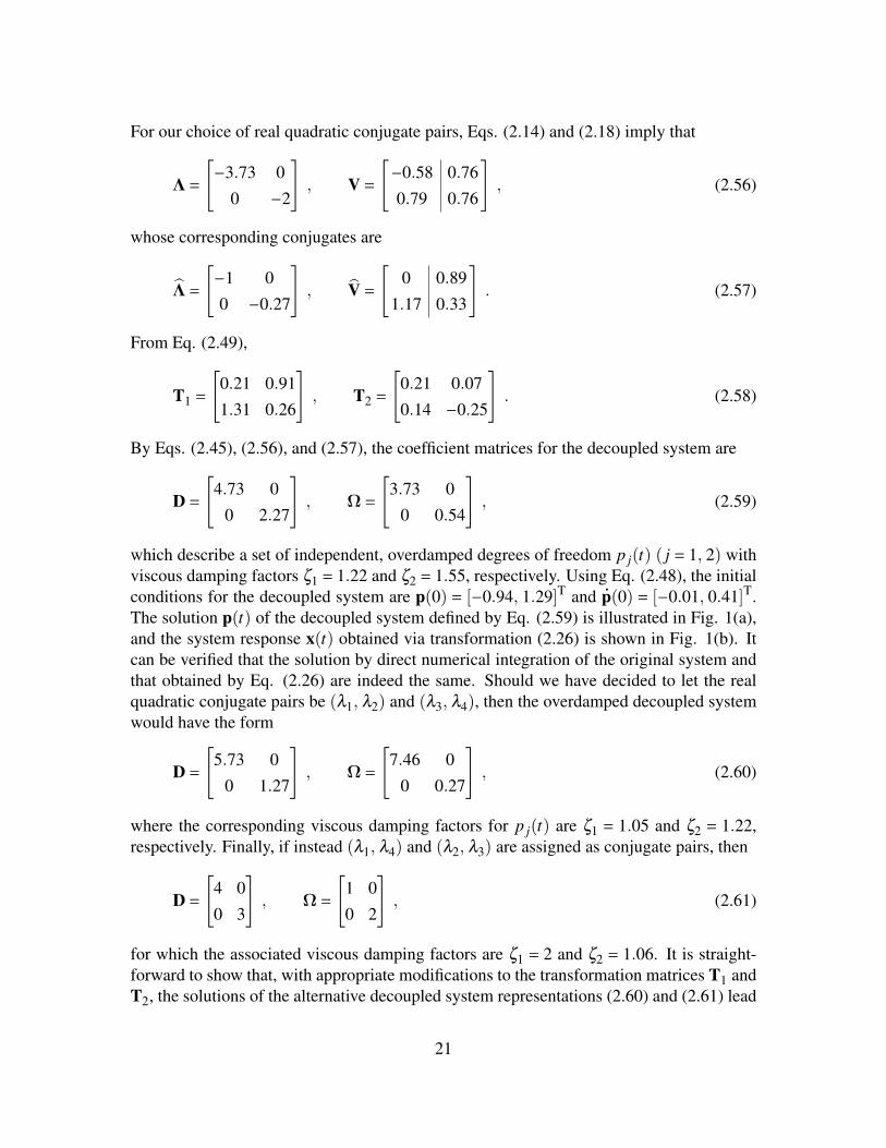
which describe a set of independent, overdamped degrees of freedom p j(t) ( j = 1, 2) withviscous damping factors ζ1 = 1.22 and ζ2 = 1.55, respectively. Using Eq. (2.48), the initialconditions for the decoupled system are p(0) = [−0.94, 1.29]T and

.p(0) = [−0.01, 0.41]T.

The solution p(t) of the decoupled system defined by Eq. (2.59) is illustrated in Fig. 1(a),and the system response x(t) obtained via transformation (2.26) is shown in Fig. 1(b). Itcan be verified that the solution by direct numerical integration of the original system andthat obtained by Eq. (2.26) are indeed the same. Should we have decided to let the realquadratic conjugate pairs be (λ1, λ2) and (λ3, λ4), then the overdamped decoupled systemwould have the form

D =[

5.73 0

0 1.27

], Ω=

[7.46 0

0 0.27

], (2.60)

where the corresponding viscous damping factors for p j(t) are ζ1 = 1.05 and ζ2 = 1.22,respectively. Finally, if instead (λ1, λ4) and (λ2, λ3) are assigned as conjugate pairs, then

D =[

4 0

0 3

], Ω=

[1 0

0 2

], (2.61)

for which the associated viscous damping factors are ζ1 = 2 and ζ2 = 1.06. It is straight-forward to show that, with appropriate modifications to the transformation matrices T1 andT2, the solutions of the alternative decoupled system representations (2.60) and (2.61) lead

21

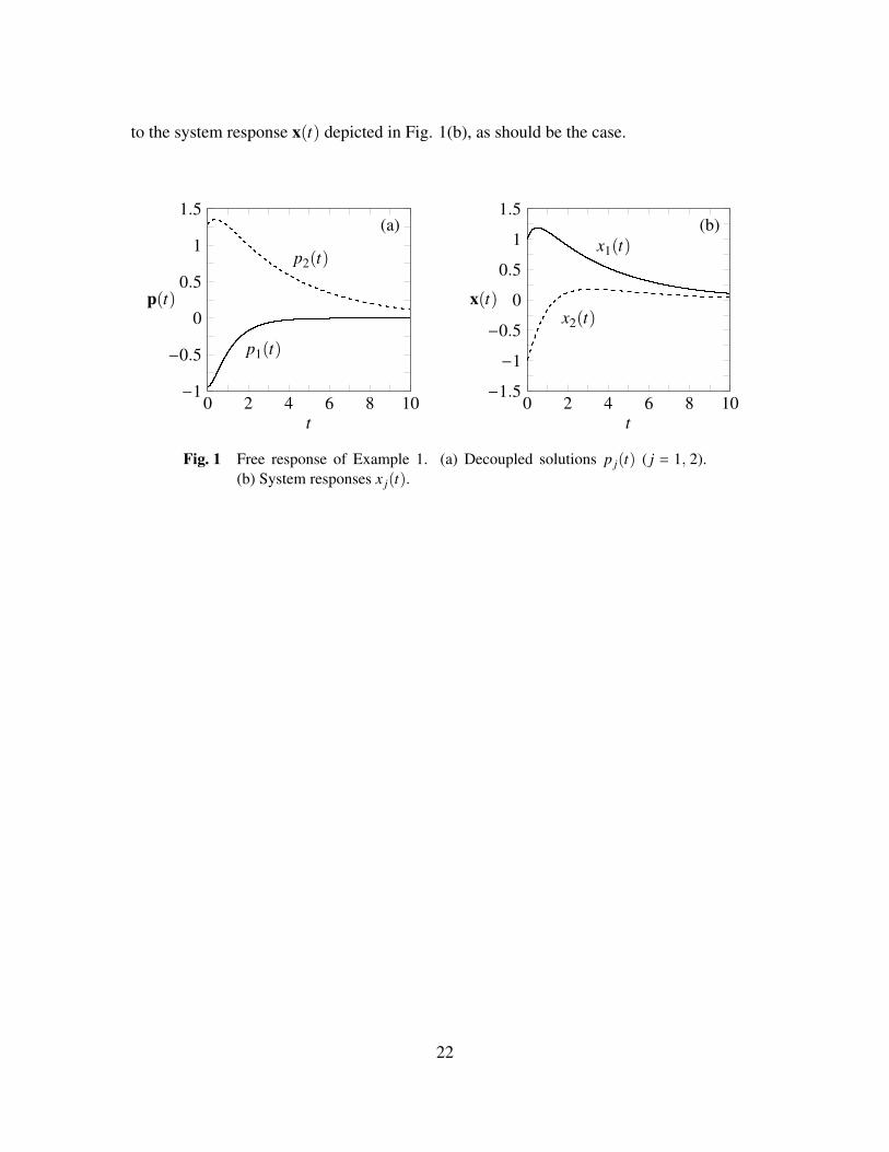
to the system response x(t) depicted in Fig. 1(b), as should be the case.

0 2 4 6 8 10−1

−0.5

0

0.5

1

1.5

p1(t)

p2(t)

(a)

t

p(t)

0 2 4 6 8 10−1.5

−1

−0.5

0

0.5

1

1.5

x1(t)

x2(t)

(b)

t

x(t)

Fig. 1 Free response of Example 1. (a) Decoupled solutions p j(t) ( j = 1, 2).(b) System responses x j(t).

22

Chapter 3Decoupling of Non-Defective Systems inForced Motion

This chapter is concerned with decoupling a forced non-defective system (1.1) intothe form (1.2) and exactly recovering the forced response x(t) from the decoupled sys-tem response p(t). For the sake of generality, we consider the case in which system (1.1)has mixed eigenvalues. Additionally, while it is possible to approach decoupling in then-dimensional configuration space, it is more convenient to perform manipulations in the2n-dimensional state space. We begin in Section 3.1 by establishing a state space repre-sentation of system (1.1) and postulating an associated solution based on the free response.Next, the relationship between the applied excitation f(t) and modal forcing g(t) is ex-plored in Section 3.2, and a transformation that recovers the forced response x(t) exactly ispresented in Section 3.3. The chapter closes with a discussion in Section 3.4 demonstratinghow the decoupling procedure developed here generalizes classical modal analysis. Themethodology presented here is largely based on [46], but we perform manipulations in thestate space in a different and more generalized manner.

3.1 State space formulation

Suppose a non-defective system (1.1) possesses a mixed eigenspectrum and is actedupon by an arbitrary external excitation f(t). It is assumed that the eigenvectors are nor-malized in accordance with Eqs. (2.42) and (2.43). We may cast system (1.1) in the non-

23

symmetric state space realization (e.g., see [52])[ .x(t)..x(t)

]=[

O I−M−1K −M−1C

][x(t).x(t)

]+[

OM−1

]f(t) . (3.1)

It is well known that the application of external forcing does not alter the fundamentalstructure of the decoupled system for the case of classical damping (e.g., see [1–3]). Thus,it is reasonable to postulate that system (1.1) is decoupled into the form (1.2) such that thecoefficient matrices D and Ω are the same as those in the case of free motion under initialexcitation (i.e., D and Ω are as defined in Eq. (2.45)). Based on this assumption and thefree response’s state space representation (2.47), define a linear time-invariant coordinatetransformation[

x(t).x(t)

]=[

V VVΛ VΛ

][I IΛ Λ

]−1[p1(t)

p2(t)

]= S

[p1(t)

p2(t)

], (3.2)

for which p1(t) and p2(t) are n-dimensional vectors whose relationships to the forcedmodal response p(t) and its associated velocity

.p(t) are to be determined. It also remains

to be seen how the modal excitation g(t) is related to the applied forcing f(t).

3.2 Transformation of the applied forcing

Inserting transformation (3.2) into the first-order formulation (3.1) and premultiplyingthe resulting state equation by S−1, we obtain[ .

p1(t).p2(t)

]=[

O I−Ω −D

][p1(t)

p2(t)

]+[

TT2

TT1 −DTT

2

]f(t) , (3.3)

where the matrices T1 and T2 are as given in Eq. (2.49). The upper and lower halves ofstate equation (3.3) are, respectively,

.p1(t)−p2(t)= TT

2 f(t) , (3.4).p2(t)+Dp2(t)+Ωp1(t)= (TT

1 −DTT2 ) f(t) . (3.5)

Using Eq. (3.4) to eliminate p2(t) from Eq. (3.5) yields an equation of motion in p1(t):

..p1(t)+D

.p1(t)+Ωp1(t)= TT

1 f(t)+TT2

.f(t) . (3.6)

Comparing Eq. (3.6) to the decoupled system (1.2), it becomes clear that p1(t) correspondsto the modal displacement p(t), and thus the modal forcing g(t) is related to the applied

24

excitation f(t) by

g(t)= TT1 f(t)+TT

2.f(t) . (3.7)

While continuous differentiability of the driving force f(t) seems to be implied by Eq. (3.7),this constraint may be relaxed by treating the derivative

.f(t) in the sense of distributions

(e.g., the derivative of a unit step is a Dirac delta; see [53]).

3.3 Recovering the forced response

Combining Eqs. (3.2) and (3.4) with p1(t)= p(t), we have that the forced response x(t)of a non-defective system (1.1) with mixed eigenvalues is related to the modal responsep(t) by the state equation[

x(t).x(t)

]=[

V VVΛ VΛ

][I IΛ Λ

]−1[p(t)

.p(t)−TT

2 f(t)

], (3.8)

and hence the modal initial conditions p(0) and.p(0) are calculated from the system initial

conditions x(0) and.x(0) according to[

p(0).p(0)

]=[

I IΛ Λ

][V V

VΛ VΛ

]−1[x(0).x(0)

]+[

0TT

2 f(0)

]. (3.9)

As in the case of free vibration, it is possible to extract an analytical expression from thestate space transformation (3.8) that recovers the forced response x(t) directly. Isolatingthe upper half of Eq. (3.8) gives

x(t)= T1 p(t)+T2.p(t)−T2TT

2 f(t) . (3.10)

It is interesting to note that transformation (3.10) depends continuously on the driving forcef(t) and constitutes a nonlinear mapping between x(t) and p(t).

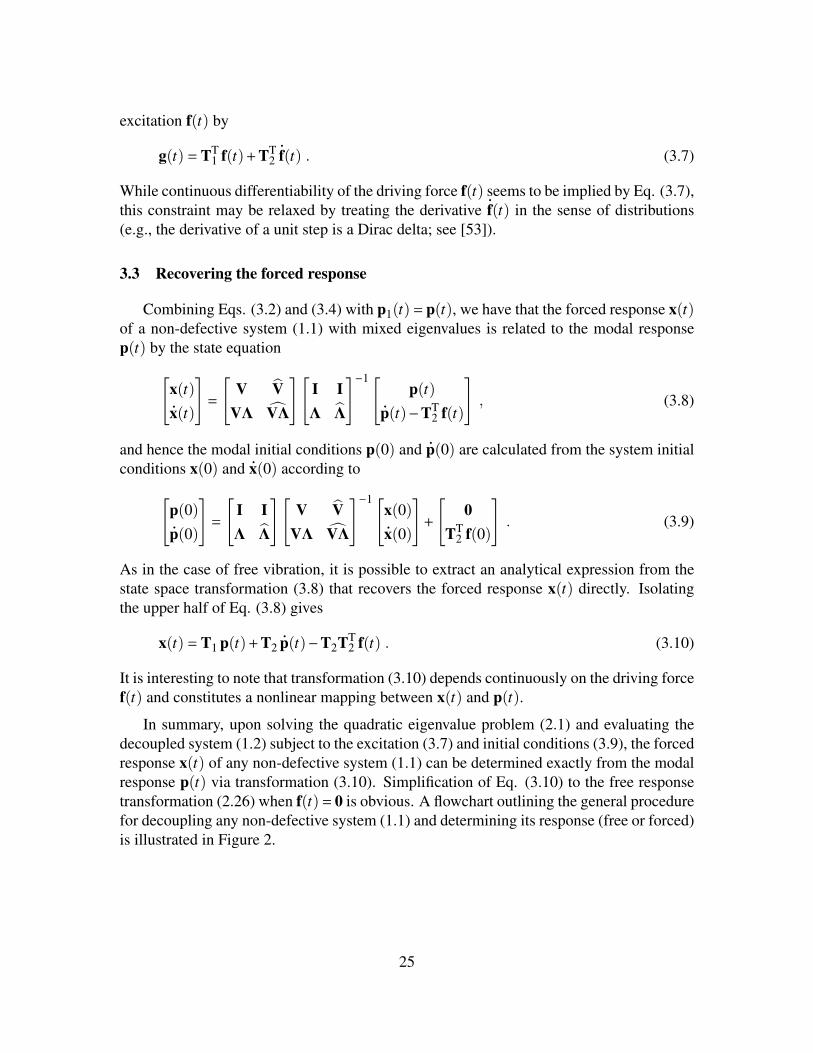
In summary, upon solving the quadratic eigenvalue problem (2.1) and evaluating thedecoupled system (1.2) subject to the excitation (3.7) and initial conditions (3.9), the forcedresponse x(t) of any non-defective system (1.1) can be determined exactly from the modalresponse p(t) via transformation (3.10). Simplification of Eq. (3.10) to the free responsetransformation (2.26) when f(t)= 0 is obvious. A flowchart outlining the general procedurefor decoupling any non-defective system (1.1) and determining its response (free or forced)is illustrated in Figure 2.

25

Coupled linear systemM

..x(t)+C

.x(t)+Kx(t)= f(t)

with coordinate x(t)

Solve(Mλ

2 +Cλ +K)v = 0

Normalize vk, vk (k = 1, 2, . . . , n):

2λkvk · (Mvk)+vk · (Cvk)= λk − λk

2λkvk · (Mvk)+ vk · (Cvk)= λk −λk

Construct

Λ=n⊕

k = 1

λk

V =[

v1 · · · vn

]and their conjugates

Construct

D =−(Λ+ Λ)Ω=ΛΛ

T1 = (VΛ− VΛ)(Λ−Λ)−1

T2 = (V−V)(Λ−Λ)−1

g(t)= TT1 f(t)+TT

2.f(t)

Decoupled linear system..p(t)+D

.p(t)+Ωp(t)= g(t)

with coordinate p(t)

Eq. (3.10)

Fig. 2 Flowchart for decoupling and response calculation of any non-defectivelinear dynamical system in free or forced motion. This flowchart is basedon Figure 1 in [46].

26

3.4 Reduction to classical modal analysis

We now demonstrate how the decoupling methodology developed in this chapter rep-resents a direct generalization of classical modal analysis. Suppose the eigenvectors ofsystem (1.1) are normalized in accordance with Eqs. (2.42) and (2.43). Should system(1.1) be classically damped, then among the (2r)!/(2rr!) different ways to pair the realeigenvalues, there is a particular pairing scheme such that the matrix V of eigenvectorsand its conjugate coincide with the modal matrix U containing the eigenvectors of the un-damped system: V= V=U. Consequently, the transformation matrices T1 =U and T2 =O,and hence Eqs. (3.8) and (3.7) reduce to the coordinate transformation x(t) = Up(t) andexcitation g(t) = UT f(t), respectively, that are indicative of classical modal analysis. Ofcourse, reduction to classical modal analysis occurs regardless of eigenvector normaliza-tion, with multiplicative constants appearing here and there if normalizations (2.42) and(2.43) are not used.

3.5 Efficiency of the decoupling algorithm

The utility of an algorithm is often based not only on how well it performs a desiredtask, but also on how efficiently it does so. To motivate the acceptance and widespreaduse of the decoupling algorithm illustrated in Figure 2, its efficiency should be examinedand compared to that of direct numerical integration of system (1.1). Here we assumethat the system response x(t) and applied forcing f(t) are sufficiently smooth. Countingthe number of floating point operations (flops) executed by an algorithm is one way ofmeasuring its performance. For direct numerical integration, typically the n-degree-of-freedom system (1.1) is transformed into the first-order form (3.1) and then discretized intoa difference equation with m time steps, from which the response x(t) can be solved forthrough recursion (e.g., see [3, 52, 54]). An estimate of the flop count for this procedureis [55–57]

N1 = 160n3 +16mn2 , (3.11)

where mÀ n in general. Using the decoupling algorithm outlined in Figure 2, the quadraticeigenvalue problem (2.1) is solved, the decoupled system (1.2) is then constructed, theresponse of each independent subsystem is obtained through direct numerical integrationvia discretization, and finally the system response x(t) is recovered from transformation(3.10). An estimate of the flop count for the decoupling algorithm is [55–57]

N2 = 213n3 + (10m+4)n2 +16mn . (3.12)

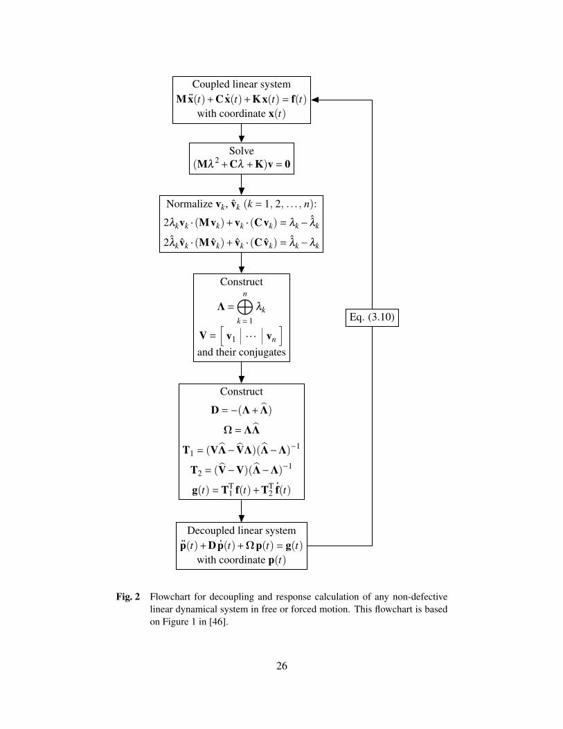
Figure 3 illustrates how the flop count estimates N1 and N2 scale with the size of system(1.1) for m = 106 time instants. As shown, solution of system (1.1) using the decouplingalgorithm in Figure 2 is more efficient than by direct numerical integration, and this is trueso long as there are approximately m > 4000 time instants.

27

0 100 200 300 400 5000

1

2

3

4

N1

N2

n

Flops

×1012

Fig. 3 Comparison of the estimated flops for solution of a non-defective system(1.1) with n degrees of freedom using direct numerical integration via dis-cretization (N1) and using the decoupling algorithm (N2) illustrated in Fig-ure 2. The number of time instants is m = 106. This diagram is adaptedfrom Figure 2 in [46].

3.6 An illustrative example

Here we provide a numerical example illustrating the decoupling procedure for a forcednon-defective system of the type (1.1). We focus on a system that has complex and realeigenvalues to demonstrate the method by which a system with mixed damping charac-teristics is decoupled. Refer to [46] for additional examples of decoupling non-defectivesystems in forced motion.

Example 2

Suppose a non-classically damped, 2-degree-of-freedom system with mass matrix M =I2 has damping matrix C, stiffness matrix K, and excitation f(t) given by

C =[

3 −1

−1 4

], K =

[2 −1

−1 5

], f(t)=

[1

0

]sint . (3.13)

Take as initial conditions x(0) = [1, 0]T and.x(0) = [1, −1]T. Solution of the associated

quadratic eigenvalue problem reveals that the system is non-defective and has mixed eigen-values:

λ1 = λ 2 =−1.5+ i 0.87 , λ3 =−3 , λ4 =−1 , (3.14)

28

for which the corresponding eigenvectors vi (i = 1, 2, 3, 4), normalized according to Eqs.(2.42) and (2.43), are

v1 = v2 =[

0.76e−i 45

−0.76e−i 165

], v3 =

[0.82

−0.82

], v4 =

[1.41

0

]. (3.15)

By Eqs. (2.14) and (2.18),

Λ=[−1.5+ i 0.87 0

0 −3

], V =

[0.76e−i 45 0.82

−0.76e−i 165 −0.82

], (3.16)

where the associated conjugates are given by

Λ=[−1.5− i 0.87 0

0 −1

], V =

[0.76ei 45 1.41

−0.76ei 165 0

]. (3.17)

It follows from Eq. (2.49) that

T1 =[−0.39 1.71

1.07 0.41

], T2 =

[−0.62 0.30

0.23 −0.41

]. (3.18)

From Eqs. (2.45), (3.16), and (3.17), the decoupled system’s coefficient matrices are

D =[

3 0

0 4

], Ω= 3 I2 , (3.19)

implying that the degree of freedom p1(t) is underdamped with viscous damping factorζ1 = 0.87, while p2(t) is overdamped with ζ2 = 1.15. The corresponding initial conditionsare p(0) = [−1.47, 0.90]T and

.p(0) = [2.54, 1.55]T from Eq. (3.9). The modal excitation

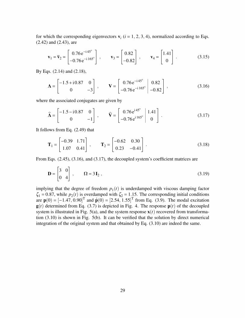
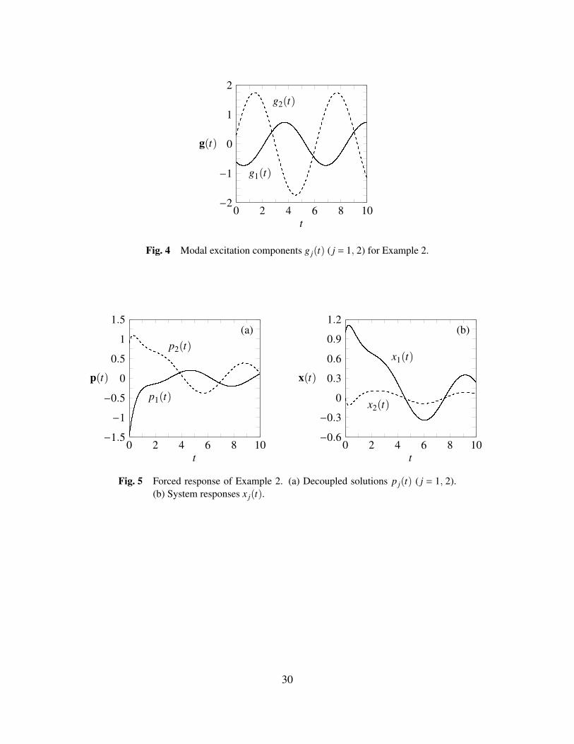
g(t) determined from Eq. (3.7) is depicted in Fig. 4. The response p(t) of the decoupledsystem is illustrated in Fig. 5(a), and the system response x(t) recovered from transforma-tion (3.10) is shown in Fig. 5(b). It can be verified that the solution by direct numericalintegration of the original system and that obtained by Eq. (3.10) are indeed the same.

29

0 2 4 6 8 10−2

−1

0

1

2

g1(t)

g2(t)

t

g(t)

Fig. 4 Modal excitation components g j(t) ( j = 1, 2) for Example 2.

0 2 4 6 8 10−1.5

−1

−0.5

0

0.5

1

1.5

p1(t)

p2(t)(a)

t

p(t)

0 2 4 6 8 10−0.6

−0.3

0

0.3

0.6

0.9

1.2

x1(t)

x2(t)

(b)

t

x(t)

Fig. 5 Forced response of Example 2. (a) Decoupled solutions p j(t) ( j = 1, 2).(b) System responses x j(t).

30

Chapter 4Decoupling of Defective Systems in FreeMotion

In this chapter, we present a method by which an unforced defective system (1.1) (i.e.,f(t) = 0) is decoupled into the form (1.2) with g(t) = 0 and the free response x(t) is re-covered exactly from the decoupled system response p(t). We begin with a discussion ofthe quadratic eigenvalue problem for defective systems in Section 4.1. Next, we developa generalized decoupling transformation in Section 4.2 via analysis in state space, and therelationship between the state space representations of the original and decoupled systemsis briefly explored in Section 4.3. To streamline the introduction of new details, an as-sumption regarding the defective eigenvalues of system (1.1) is made in Section 4.4 forconvenience. We illustrate how the generalized decoupling procedure outlined in Section4.2 is applied to defective systems with complex eigenvalues in Section 4.5, and we fol-low this with an application to the case of defective real eigenvalues in Section 4.6. Whilethe decoupling of systems in free motion with defective complex eigenvalues was brieflytouched upon in [45], we provide an alternative and more in-depth analysis here. We dis-cuss in Section 4.7 how the decoupling procedure is affected when the constraint imposedin Section 4.4 is relaxed. We conclude the chapter by demonstrating in Section 4.8 how thedecoupling methodology described here reduces to classical modal analysis when system(1.1) is classically damped.

31

4.1 The quadratic eigenvalue problem

In the event that system (1.1) is defective, solution of the quadratic eigenvalue problem(2.1) reveals that some of the eigenvalues are repeated and do not have associated withthem a full complement of linearly independent eigenvectors. Such eigenvalues are termeddefective. As an example, an eigenvalue that is repeated more than n times is necessarilydefective. Let λk denote the kth eigenvalue of system (1.1), and suppose it is defective. Thenumber of times the defective eigenvalue λk is repeated is referred to as its algebraic multi-plicity mk. Considering the quadratic matrix pencil Q(λ ) = Mλ

2 +Cλ +K, the geometricmultiplicity ρk of the defective eigenvalue λk is given by the dimension of the null spaceof Q(λk), and hence it is equivalent to the number of linearly independent eigenvectors as-sociated with λk. For obvious reasons, the geometric multiplicity cannot exceed either thealgebraic multiplicity mk or the system order n, whichever is smaller: ρk 6min(mk,n). Theassociated ρk eigenvectors vk

j ( j = 1, 2, . . . , ρk) are supplemented with mk −ρk generalizedeigenvectors to form a complete set of vectors for λk, where the final eigenvector vk

ρkand

the generalized eigenvectors constitute a Jordan chain of length mk −ρk +1 characterizedby the recursive scheme (see [50])

0 = Q(λk)vkρk

,

0 = Q(λk)vkρk+1 +Q′(λk)vk

ρk,

0 = Q(λk)vkρk+2 +Q′(λk)vk

ρk+1 +12

Q′′(λk)vkρk

,

...

0 = Q(λk)vkmk

+Q′(λk)vkmk−1 +

12

Q′′(λk)vkmk−2 .

(4.1)

In the above sequence, Q′(λk) and Q′′(λk) denote the first and second derivatives of Q(λ ),respectively, with respect to λ and evaluated at the defective eigenvalue λk:

Q′(λk)=dQ(λ )

dλ

∣∣∣∣∣λ =λk

= 2Mλk +C , (4.2)

Q′′(λk)=d2Q(λ )

dλ2

∣∣∣∣∣λ =λk

= 2M . (4.3)

Regardless of the nature of the system’s eigenspectrum, the free response x(t) of system(1.1) may be cast in the general matrix-vector form (e.g., see [48, 49])

x(t)= Vx eJxtc , (4.4)

for which Jx is an order 2n Jordan matrix with the system eigenvalues on the diagonal, Vxis an n×2n matrix of the associated eigenvectors and generalized eigenvectors, and c is a

32

2n-dimensional vector of coefficients determined from the initial conditions x(0) and.x(0).

Writing Eq. (4.4) and its derivative in the form of a state equation,[x(t).x(t)

]=[

Vx

Vx Jx

]eJxtc = Sx eJxtc , (4.5)

where the order 2n matrix Sx is invertible since Jx and Vx constitute a Jordan pair. If system(1.1) is non-defective, the Jordan matrix Jx is diagonal and every eigenvalue (repeatedor not) has a corresponding eigenvector, and thus Eq. (4.4) reduces to the eigensolutionsummation (2.2). However, when system (1.1) is defective, the Jordan decomposition (4.4)is the only available representation of the free response x(t).

4.2 A generalized state space representation

Defective or not, we assume that system (1.1) may be decoupled into the form (1.2)such that the diagonal coefficient matrices D and Ω are always given by Eq. (2.45), wherethe arrangement of eigenvalues in the diagonal matrix Λ and its conjugate Λ is dependenton the choice of eigensolution pairing. We have demonstrated previously that it is possibleto decouple a non-defective system (1.1) while preserving both the algebraic and geometricmultiplicities of the associated eigenvalues (i.e., the decoupling transformation is strictlyisospectral). If one insists that geometric multiplicities be preserved, then a defective sys-tem (1.1) may only be partially decoupled [58]. Our main goal is to demonstrate howdefective systems can be decoupled, at any cost, by not requiring geometric multiplicitiesto be preserved.

Since phase synchronization for a non-defective system (1.1) does not disturb the eigen-solution coefficients, we shall construct the decoupling transformation for a defective sys-tem (1.1) so that it also preserves these coefficients. Consequently, the modal response p(t)may be cast in a matrix-vector form analogous to Eq. (4.4):

p(t)= Vp eJptc . (4.6)

Here, Jp is an order 2n Jordan matrix consisting of the system eigenvalues, but it maynot necessarily be the same as Jx. The matrix Jp has the same diagonal elements (i.e.,the eigenvalues) as Jx, but the off-diagonal elements are generally different since we donot impose preservation of geometric multiplicities. The matrix Vp is an n×2n matrix ofvectors that essentially pairs the eigensolutions according to a specified pairing scheme.Expressing Eq. (4.6) and its derivative as a state equation,[

p(t).p(t)

]=[

Vp

Vp Jp

]eJptc = Sp eJptc , (4.7)

33

where the order 2n matrix Sp will always be invertible so long as eigenvalues are paired topreserve the second-order structure of the equation of motion (1.1). Combining Eqs. (4.5)and (4.7), the response x(t) of system (1.1) is recovered from the modal response p(t) inthe state space according to[

x(t).x(t)

]=[

Vx

Vx Jx

]eJxt e−Jpt

[Vp

Vp Jp

]−1[p(t).p(t)

]= Sx eJxt e−Jpt S−1

p

[p(t).p(t)

], (4.8)

and thus the modal initial conditions p(0) and.p(0) are connected to the system initial

conditions x(0) and.x(0) by the state equation[

p(0).p(0)

]=[

Vp

Vp Jp

][Vx

Vx Jx

]−1[x(0).x(0)

]. (4.9)

A generalized procedure for decoupling system (1.1) into the form (1.2) and recoveringthe response x(t) from the decoupled solution p(t) via state space transformation is summa-rized as follows. (i) Solve the quadratic eigenvalue problem (2.1) to determine the systemeigenvalues and eigenvectors. If system (1.1) is defective, additional analysis is required toobtain generalized eigenvectors as needed. (ii) Based on the nature of the system’s eigen-spectrum, specify an appropriate eigenvalue pairing scheme, and arrange the eigenvaluesaccordingly in the diagonal matrix Λ and its conjugate Λ. (iii) Construct the matrices Jxand Vx from the system eigenvalues, eigenvectors, and generalized eigenvectors. (iv) Formthe matrices Jp and Vp such that the solution p(t) of the decoupled system (1.2) satisfies thespecified pairing scheme. (v) Obtain the initial conditions p(0) and

.p(0) for the decoupled

system via transformation (4.9). (vi) Construct the coefficient matrices D and Ω in accor-dance with Eq. (2.45), and then determine the response p(t) of the decoupled system. (vii)Retrieve the response x(t) from the decoupled solution p(t) using transformation (4.8).

The heart of the decoupling procedure described herein lies in steps (ii) through (iv).To illustrate, we shall demonstrate how the above procedure relates to the decoupling ofa non-defective system (1.1) with mixed eigenvalues (2c complex and the remaining 2rreal) as presented in Chapter 2. Because the eigenvalues are generally semi-simple (i.e.,they may be repeated but have corresponding eigenvectors), they may be paired as complexand real quadratic conjugates to yield c underdamped and r overdamped (not necessarilydistinct) decoupled degrees of freedom, respectively. Consequently, the c complex andr real eigenvalues and eigenvectors (that constitute the c complex conjugate and r realquadratic conjugate pairs, respectively) may be arranged in some order in the matrices Λand V, respectively, in accordance with Eqs. (2.14) and (2.18). Comparing the summationrepresentation of the response x(t) given in Eq. (2.44) to the general form (4.4), it is clearthat

Jx =Λ⊕ Λ , Vx =[

V V]. (4.10)

34

The decoupled solutions pk(t) given by Eq. (2.46) imply that

Jp = Jx , Vp =[

I I]

(4.11)

in Eq. (4.6). As a result, Eqs. (4.8) and (4.9) reduce to the familiar transformations (2.47)and (2.48), respectively, for a non-defective system (1.1). There currently does not existcriteria for eigenvalue pairing when system (1.1) is defective. Put another way, it is notclear how to form Λ and its conjugate Λ when the eigenvalues are defective in order toconstruct the coefficient matrices D and Ω that define the decoupled system (1.2). Thischapter presents a solution to this problem.

4.3 State transformation of the equation of motion

Suppose we cast an unforced system (1.1) and its decoupled form (1.2), respectively, inthe nonsymmetric state space realizations[ .

x(t)..x(t)

]=[

O I−M−1K −M−1C

][x(t).x(t)

]= A

[x(t).x(t)

], (4.12)

[ .p(t)..p(t)

]=[

O I−Ω −D

][p(t).p(t)

]= B

[p(t).p(t)

]. (4.13)

Since the eigenvalues of system (1.1) and their algebraic multiplicities are preserved duringdecoupling, the nonsymmetric order 2n matrices A and B have the same eigenvalues (i.e.,they are isospectral), but the corresponding geometric multiplicities may be different (thatis, A and B are not strictly isospectral), which is reflected in the associated Jordan matricesJx and Jp, respectively.

In the general case of a defective system (1.1), what is the real transformation thatconverts its state space representation (4.12) into Eq. (4.13), from which the decoupledsystem (1.2) is extracted? In other words, how are the matrices A and B related? To answerthis question, begin by writing the general state space transformation (4.8) in the morecompact form[

x(t).x(t)

]= Sx eJxt e−Jpt S−1

p

[p(t).p(t)

]= S(t)

[p(t).p(t)

]. (4.14)

35

Substitute the state vector (4.14) and its derivative into Eq. (4.12) and then premultiply theresulting equation by S−1(t) to obtain[ .

p(t)..p(t)

]=(

S−1(t)AS(t)−S−1(t).S(t)

)[p(t).p(t)

]. (4.15)

Comparing Eqs. (4.13) and (4.15) reveals that the constant matrices A and B are related bythe time-dependent transformation

B = S−1(t)AS(t)−S−1(t).S(t) . (4.16)

Time variation in Eq. (4.16) is a direct result of not requiring that geometric multiplici-ties be preserved during decoupling. In other words, transformation (4.16) is time-varyingwhen the Jordan matrices Jx and Jp are not identical. In the event that Jx = Jp, the matrixS(t) = S is independent of time t, and hence Eq. (4.16) reduces to the similarity transfor-mation B = S−1AS. One situation for which this reduction occurs is when system (1.1) isnon-defective, in which case the constant matrix S is given by the order 2n transformationin state equation (2.47). This similarity transformation was implied in Eqs. (3.1)-(3.3)when decoupling of non-defective systems in forced vibration was addressed.

4.4 Restriction on the geometric multiplicity

To streamline our subsequent discussion of decoupling defective systems, it will be as-sumed that every defective eigenvalue λk of system (1.1) has unit geometric multiplicity(i.e., ρk = 1), and hence the length of its associated Jordan chain is given by the algebraicmultiplicity mk. In the case of defective complex eigenvalues, relaxation of this constraintleads to a trivial modification of the decoupling procedure. When system (1.1) possessesdefective real eigenvalues, however, the situation is more delicate and requires some dis-cussion.

4.5 Complex eigenvalues

Suppose that solution of the quadratic eigenvalue problem (2.1) reveals that the 2neigenvalues of system (1.1) are complex and defective. As the system matrices M, C, andK are real, these eigenvalues necessarily form nc complex conjugate pairs, where 2nc < 2n.Let mk (k = 1, 2, . . . , nc) be the algebraic multiplicity of the defective complex eigenvalueλk. Then mk is also the algebraic multiplicity of the complex conjugate eigenvalue λ k sothat m1+·· ·+mnc

= n. Under the assumption of unit geometric multiplicity, each defectiveeigenvalue λk has a single (complex) eigenvector vk

1 associated with it. Let Jk be a Jordan

36

block of order mk formed from the defective eigenvalue λk:

Jk =

λk 1 0 · · · 0

0 λk 1 · · · 0... . . . . . . . . . ...

0 · · · 0 λk 1

0 · · · 0 0 λk

. (4.17)

In addition, construct an n×mk matrix Vk whose columns contain the single eigenvector vk1

and the mk −1 generalized eigenvectors that constitute the mk-long Jordan chain associatedwith λk, and take ck to be an mk-dimensional vector consisting of the complex coefficientsck

j ( j = 1, 2, . . . , mk) for the corresponding eigensolutions:

Vk =[

vk1 · · · vk

mk

], ck =

[ck

1 · · · ckmk

]T. (4.18)

Expressing the general form (4.4) of the free response x(t) in terms of the Jordan pairs(Jk,Vk) and their complex conjugates,

x(t)=nc∑

k = 1

(Vk eJktck +Vk eJktck

). (4.19)

If system (1.1) is non-defective and it possesses a complex eigenvalue λk repeated mktimes, then associated with λk are mk independent underdamped oscillators that executeoscillatory free motion, governed by the equation of motion (1.2), with identical decayrate αk and damped frequency ωk. The initial conditions, however, are generally differ-ent because the eigensolution coefficients ck are typically not the same. In progressing todefective oscillatory systems, each defective complex eigenvalue λk with algebraic multi-plicity mk yields mk identical and independent underdamped systems subject to differentsets of initial conditions upon decoupling. Specifically, every decoupled coordinate pk

j(t)( j = 1, 2, . . . , mk) corresponding to the defective eigenvalue λk satisfies the same equationof motion

..pk

j(t)− (λk +λ k).pk

j(t)+λkλ k pkj(t)= 0 , (4.20)

for which the solution pkj(t) is of the form

pkj(t)= ck

jeλkt +ck

jeλ kt . (4.21)

37

The decoupled equation of motion (4.20) implies that the nc eigenvalues (that constitutethe nc complex conjugate pairs) may be arranged in the diagonal matrix Λ according to

Λ=nc⊕

k = 1

Λk , Λk = λk Imk. (4.22)

The (complex) conjugate of Λ immediately follows. Given Eq. (4.22) and its conjugate,we may then construct the coefficient matrices D and Ω in accordance with Eq. (2.45) toestablish the decoupled system (1.2). Equation (4.22) permits us to write the Jordan block(4.17) in the form Jk = Λk +Nk, where Nk is an order mk nilpotent matrix of 1’s on thesuperdiagonal. Comparing Eqs. (4.4) and (4.19) reveals that

Jx = J⊕J , Vx =[

V V], (4.23)

where the order n block diagonal matrix J and the n× n matrix V of eigenvectors andgeneralized eigenvectors are given by, respectively,

J =nc⊕

k = 1

Jk =Λ+N , V =[

V1 · · · Vnc

]. (4.24)

Based on the arrangement of eigenvalues in Λ, the modal response vector p(t) has theconformable structure

p(t)=[

pT1 (t) · · · pT

nc(t)]T

, pk(t)=[

pk1(t) · · · pk

mk(t)]T

, (4.25)

from which we deduce that

Jp =Λ⊕Λ , Vp =[

I I]

(4.26)

in order to satisfy the response (4.21) for each decoupled coordinate pkj(t). In addition,

it can be shown, by exploiting the commutativity of Λk = λk Imkand Nk in multiplication,

that eJxte−Jpt = eNt ⊕ eNt . Consequently, the state space formulation (4.8) for defectiveoscillatory motion has the equivalent time-dependent representations[

x(t).x(t)

]=[

V VVJ VJ

][eNt OO eNt

][I IΛ Λ

]−1[p(t).p(t)

]

=[

V VVJ VJ

][I IΛ Λ

]−1[eNt OO eNt

][p(t).p(t)

].

(4.27)

38

The modal and system initial conditions are related by the state equation[p(0).p(0)

]=[

I IΛ Λ

][V VVJ VJ

]−1[x(0).x(0)

]. (4.28)

As with non-defective systems, it is possible to isolate an order n transformation from thestate space representation (4.27) to directly give the response x(t):

x(t)= T1 eNt p(t)+T2 eNt .p(t) , (4.29)

where the transformation matrices T1 and T2 are as defined in Eq. (2.27). Thus, uponcalculating the modal initial conditions p(0) and

.p(0) from Eq. (4.28), the free response

pkj(t) for each decoupled coordinate may be evaluated exactly as

pkj(t)= eαkt

[pk

j(0)cosωkt + .

pkj(0)−αk pk

j(0)ωk

sinωkt

], (4.30)

from which the response x(t) of system (1.1) can be obtained directly via transformation(4.29). In addition to the quadratic eigenvalue problem (2.1), it becomes necessary toevaluate the recursive scheme (4.1) to obtain all parameters required for retrieving the freeresponse x(t) from Eq. (4.29).

In summary, if the coupled n-degree-of-freedom system (1.1) is defective with nc pairsof complex conjugate eigenvalues of respective algebraic multiplicity mk, then it may bedecoupled into n underdamped degrees of freedom corresponding to nc collections of mkidentical, underdamped single-degree-of-freedom oscillators subject to different initial con-ditions. In the event that system (1.1) is non-defective, the nilpotent matrix N=O, and thusthe Jordan matrix J =Λ. As a result, Eqs. (4.27)-(4.29) reduce to transformations (2.23),(2.24), and (2.26), respectively, associated with non-defective complex eigenvalues, as ex-pected.

The partitioning of the order 2n transformation matrices in state equation (4.27) intoblocks of size n makes it convenient to look further into the mechanics of transformation(4.16) and how it relates the state matrices A and B of the nonsymmetric state space realiza-tions (4.12) and (4.13), respectively. Based on Eq. (4.27), the matrix S(t) and its derivativeare given by, respectively,

S(t)=[

V VVJ VJ

][I IΛ Λ

]−1[eNt OO eNt

]= S0

[eNt OO eNt

], (4.31)

.S(t)= S0

[N OO N

][eNt OO eNt

]. (4.32)

39

Inserting Eqs. (4.31) and (4.32) into transformation (4.16) yields

B =[

e−Nt OO e−Nt

]S−10 AS0 −

[N OO N

][

eNt OO eNt

], (4.33)

where it can be verified that

S−10 AS0 =

[N I−Ω N−D

]. (4.34)

Finally, by exploiting the commutativity in blockwise multiplication of the diagonal coef-ficient matrices D and Ω with the matrix exponential eNt , it is straightforward to show thatthe resulting matrix B is indeed the order 2n state matrix in Eq. (4.13).

4.6 Real eigenvalues

Suppose that solution of the quadratic eigenvalue problem (2.1) for system (1.1) yieldsreal eigenvalues λk that are repeated and defective. By Theorem 4.2 in [48], every eigen-vector vk

j associated with a defective real eigenvalue λk satisfies

2vkj · (Mvk

j)λk +vkj · (Cvk

j)= 0 . (4.35)

However, the quadratic eigenvalue problem (2.1) implies that

λk =− vkj · (Cvk

j)

2vkj · (Mvk

j)± i

√4(vk

j · (Mvkj))(v

kj · (Kvk

j))− (vkj · (Cvk

j))2

2vkj · (Mvk

j). (4.36)

Equations (4.35) and (4.36) are simultaneously satisfied when the discriminant of Eq.(4.36) vanishes, resulting in

λk =−

√√√√ vkj · (Kvk

j)

vkj · (Mvk

j)± i 0 = αk ± i 0 . (4.37)

Thus, defective real eigenvalues are such that ωk = 0, implying that these eigenvalues cor-respond to the boundary between real vibration (complex eigenvalues) and imaginary vi-bration (non-defective real eigenvalues). Consequently, we associate defective real eigen-values with critical damping.

Critical damping in multi-degree-of-freedom systems, classically damped or not, hasbeen discussed extensively in the literature (e.g., see [59–64]). The common thread inthese works is that every defective real eigenvalue λk giving rise to a critically dampeddegree of freedom has algebraic multiplicity mk = 2. However, there is generally no reason

40

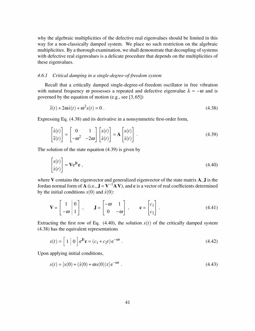
why the algebraic multiplicities of the defective real eigenvalues should be limited in thisway for a non-classically damped system. We place no such restriction on the algebraicmultiplicities. By a thorough examination, we shall demonstrate that decoupling of systemswith defective real eigenvalues is a delicate procedure that depends on the multiplicities ofthese eigenvalues.

4.6.1 Critical damping in a single-degree-of-freedom system

Recall that a critically damped single-degree-of-freedom oscillator in free vibrationwith natural frequency ω possesses a repeated and defective eigenvalue λ = −ω and isgoverned by the equation of motion (e.g., see [3, 65])

..x(t)+2ω

.x(t)+ω

2x(t)= 0 . (4.38)

Expressing Eq. (4.38) and its derivative in a nonsymmetric first-order form,[ .x(t)..x(t)

]=[

0 1

−ω2 −2ω

][x(t).x(t)

]= A

[x(t).x(t)

]. (4.39)

The solution of the state equation (4.39) is given by[x(t).x(t)

]= VeJtc , (4.40)

where V contains the eigenvector and generalized eigenvector of the state matrix A, J is theJordan normal form of A (i.e., J=V−1AV), and c is a vector of real coefficients determinedby the initial conditions x(0) and

.x(0):

V =[

1 0

−ω 1

], J =

[−ω 1

0 −ω

], c =

[c1

c2

]. (4.41)

Extracting the first row of Eq. (4.40), the solution x(t) of the critically damped system(4.38) has the equivalent representations

x(t)=[

1 0]

eJtc = (c1 +c2t)e−ωt . (4.42)

Upon applying initial conditions,

x(t)= [x(0)+ (.x(0)+ωx(0))t]e−ωt . (4.43)

41

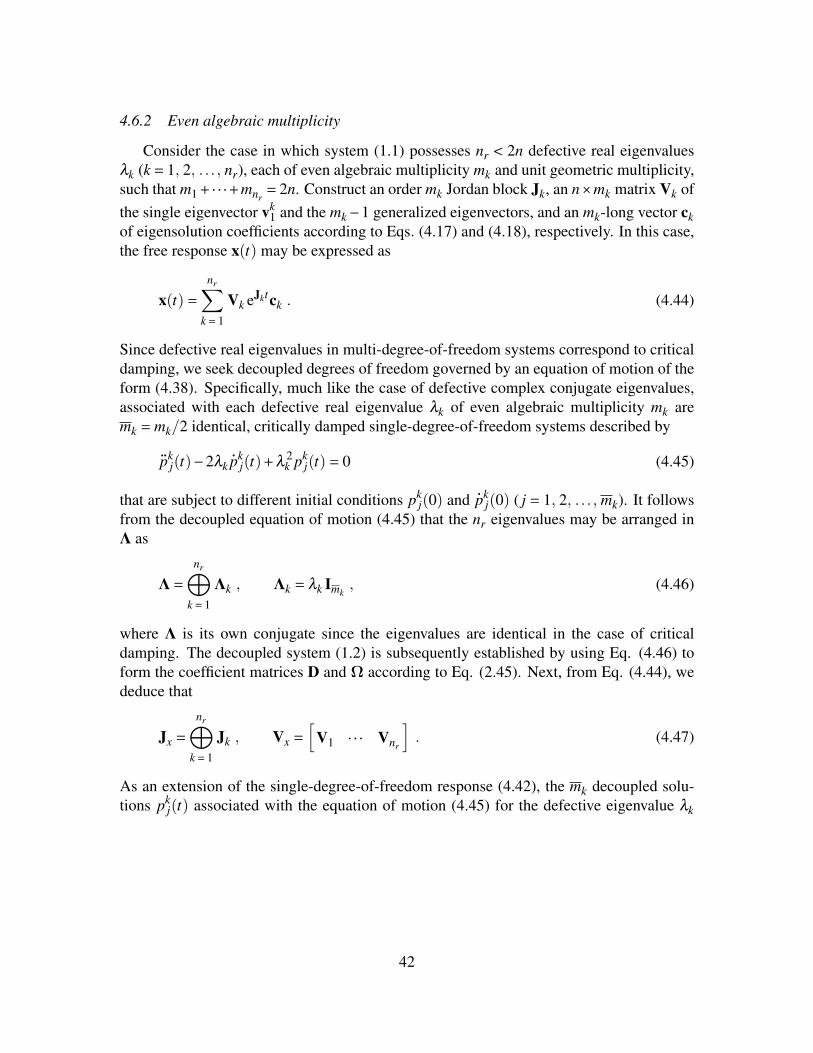
4.6.2 Even algebraic multiplicity

Consider the case in which system (1.1) possesses nr < 2n defective real eigenvaluesλk (k = 1, 2, . . . , nr), each of even algebraic multiplicity mk and unit geometric multiplicity,such that m1+·· ·+mnr

= 2n. Construct an order mk Jordan block Jk, an n×mk matrix Vk ofthe single eigenvector vk

1 and the mk −1 generalized eigenvectors, and an mk-long vector ckof eigensolution coefficients according to Eqs. (4.17) and (4.18), respectively. In this case,the free response x(t) may be expressed as

x(t)=nr∑

k = 1

Vk eJktck . (4.44)

Since defective real eigenvalues in multi-degree-of-freedom systems correspond to criticaldamping, we seek decoupled degrees of freedom governed by an equation of motion of theform (4.38). Specifically, much like the case of defective complex conjugate eigenvalues,associated with each defective real eigenvalue λk of even algebraic multiplicity mk aremk = mk/2 identical, critically damped single-degree-of-freedom systems described by

..pk

j(t)−2λk.pk

j(t)+λ2k pk

j(t)= 0 (4.45)

that are subject to different initial conditions pkj(0) and

.pk

j(0) ( j = 1, 2, . . . , mk). It followsfrom the decoupled equation of motion (4.45) that the nr eigenvalues may be arranged inΛ as

Λ=nr⊕

k = 1

Λk , Λk = λk Imk, (4.46)

where Λ is its own conjugate since the eigenvalues are identical in the case of criticaldamping. The decoupled system (1.2) is subsequently established by using Eq. (4.46) toform the coefficient matrices D and Ω according to Eq. (2.45). Next, from Eq. (4.44), wededuce that

Jx =nr⊕

k = 1

Jk , Vx =[

V1 · · · Vnr

]. (4.47)

As an extension of the single-degree-of-freedom response (4.42), the mk decoupled solu-tions pk

j(t) associated with the equation of motion (4.45) for the defective eigenvalue λk

42

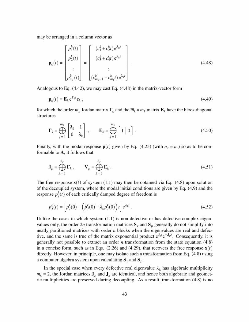
may be arranged in a column vector as

pk(t)=

pk

1(t)

pk2(t)

...

pkmk(t)

=

(ck

1 +ck2t)eλkt

(ck3 +ck

4t)eλkt

...

(ckmk−1 +ck

mkt)eλkt

. (4.48)

Analogous to Eq. (4.42), we may cast Eq. (4.48) in the matrix-vector form

pk(t)= Ek eΓktck , (4.49)

for which the order mk Jordan matrix Γk and the mk×mk matrix Ek have the block diagonalstructures

Γk =mk⊕

j = 1

[λk 1

0 λk

], Ek =

mk⊕j = 1

[1 0

]. (4.50)

Finally, with the modal response p(t) given by Eq. (4.25) (with nc = nr) so as to be con-formable to Λ, it follows that

Jp =nr⊕

k = 1

Γk , Vp =nr⊕

k = 1

Ek . (4.51)

The free response x(t) of system (1.1) may then be obtained via Eq. (4.8) upon solutionof the decoupled system, where the modal initial conditions are given by Eq. (4.9) and theresponse pk

j(t) of each critically damped degree of freedom is

pkj(t)=

[pk

j(0)+( .

pkj(0)−λk pk

j(0))

t]

eλkt . (4.52)

Unlike the cases in which system (1.1) is non-defective or has defective complex eigen-values only, the order 2n transformation matrices Sx and Sp generally do not simplify intoneatly partitioned matrices with order n blocks when the eigenvalues are real and defec-tive, and the same is true of the matrix exponential product eJxte−Jpt . Consequently, it isgenerally not possible to extract an order n transformation from the state equation (4.8)in a concise form, such as in Eqs. (2.26) and (4.29), that recovers the free response x(t)directly. However, in principle, one may isolate such a transformation from Eq. (4.8) usinga computer algebra system upon calculating Sx and Sp.

In the special case when every defective real eigenvalue λk has algebraic multiplicitymk = 2, the Jordan matrices Jp and Jx are identical, and hence both algebraic and geomet-ric multiplicities are preserved during decoupling. As a result, transformation (4.8) is no

43

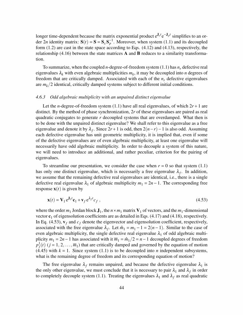
longer time-dependent because the matrix exponential product eJxte−Jpt simplifies to an or-der 2n identity matrix: S(t) = S = Sx S−1

p . Moreover, when system (1.1) and its decoupledform (1.2) are cast in the state space according to Eqs. (4.12) and (4.13), respectively, therelationship (4.16) between the state matrices A and B reduces to a similarity transforma-tion.

To summarize, when the coupled n-degree-of-freedom system (1.1) has nr defective realeigenvalues λk with even algebraic multiplicities mk, it may be decoupled into n degrees offreedom that are critically damped. Associated with each of the nr defective eigenvaluesare mk/2 identical, critically damped systems subject to different initial conditions.

4.6.3 Odd algebraic multiplicity with an unpaired distinct eigenvalue

Let the n-degree-of-freedom system (1.1) have all real eigenvalues, of which 2r+1 aredistinct. By the method of phase synchronization, 2r of these eigenvalues are paired as realquadratic conjugates to generate r decoupled systems that are overdamped. What then isto be done with the unpaired distinct eigenvalue? We shall refer to this eigenvalue as a freeeigenvalue and denote it by λ f . Since 2r+1 is odd, then 2(n−r)−1 is also odd. Assumingeach defective eigenvalue has unit geometric multiplicity, it is implied that, even if someof the defective eigenvalues are of even algebraic multiplicity, at least one eigenvalue willnecessarily have odd algebraic multiplicity. In order to decouple a system of this nature,we will need to introduce an additional, and rather peculiar, criterion for the pairing ofeigenvalues.

To streamline our presentation, we consider the case when r = 0 so that system (1.1)has only one distinct eigenvalue, which is necessarily a free eigenvalue λ f . In addition,we assume that the remaining defective real eigenvalues are identical, i.e., there is a singledefective real eigenvalue λ1 of algebraic multiplicity m1 = 2n−1. The corresponding freeresponse x(t) is given by

x(t)= V1 eJ1tc1 +v f eλ f tc f , (4.53)

where the order m1 Jordan block J1, the n×m1 matrix V1 of vectors, and the m1-dimensionalvector c1 of eigensolution coefficients are as detailed in Eqs. (4.17) and (4.18), respectively.In Eq. (4.53), v f and c f denote the eigenvector and eigensolution coefficient, respectively,associated with the free eigenvalue λ f . Let m1 = m1 −1 = 2(n−1). Similar to the case ofeven algebraic multiplicity, the single defective real eigenvalue λ1 of odd algebraic multi-plicity m1 = 2n−1 has associated with it m1 = m1/2 = n−1 decoupled degrees of freedomp1

j(t) ( j = 1, 2, . . . , m1) that are critically damped and governed by the equation of motion(4.45) with k = 1. Since system (1.1) is to be decoupled into n independent subsystems,what is the remaining degree of freedom and its corresponding equation of motion?

The free eigenvalue λ f remains unpaired, and because the defective eigenvalue λ1 isthe only other eigenvalue, we must conclude that it is necessary to pair λ1 and λ f in orderto completely decouple system (1.1). Treating the eigenvalues λ1 and λ f as real quadratic

44

conjugates, this unusual pairing implies that the remaining degree of freedom p∗(t) is ef-fectively overdamped and governed by the equation of motion

..p∗(t)− (λ1 +λ f )

.p∗(t)+λ1λ f p∗(t)= 0 . (4.54)

Consequently, by Eqs. (4.45) (with k = 1) and (4.54), the eigenvalues may be arranged inΛ and its conjugate Λ according to

Λ= λ1 Im1⊕λ1 , Λ= λ1 Im1

⊕λ f , (4.55)

from which the coefficient matrices D and Ω defining the decoupled system (1.2) may bedetermined via Eq. (2.45). A comparison of Eqs. (4.6) and (4.53) reveals that

Jx = J1 ⊕λ f , Vx =[

V1 v f

]. (4.56)

With the assistance of Eqs. (4.48)-(4.50), it is straightforward to show that the responsesp1

j(t) for the m1 critically damped degrees of freedom have the equivalent representations

p1(t)=

p1

1(t)

p12(t)

...

p1m1(t)

=

(c1

1 +c12t)eλ1t

(c13 +c1

4t)eλ1t

...

(c1m1−1 +c1

m1t)eλ1t

= E1 eΓ1tc1 , (4.57)

for which the matrices Γ1 and E1 are

Γ1 =m1⊕j = 1

[λ1 1

0 λ1

], E1 =

m1⊕j = 1

[1 0

]. (4.58)

The response p∗(t) for the overdamped degree of freedom corresponding to the equationof motion (4.54) is given by

p∗(t)= c f eλ f t +c1m1

eλ1t . (4.59)

It is important to note that the eigensolution coefficient associated with the defective eigen-value λ1 is the coefficient c1

m1that remains after having established m1 critically damped

systems. This ensures that the initial conditions for p∗(t) are independent of those for thecritically damped solutions p1

j(t). When initial conditions are applied to Eq. (4.59), theresponse p∗(t) has the form

p∗(t)=λ f p∗(0)− .

p∗(0)λ f −λ1

eλ1t −λ1 p∗(0)− .

p∗(0)λ f −λ1

eλ f t . (4.60)

45

Structuring the modal response vector as

p(t)=[

pT1 (t) p∗(t)

]T(4.61)

to be conformable to Λ, it is implied by Eqs. (4.57) and (4.59) that

Jp = Γ1 ⊕λ1 ⊕λ f , Vp = E1 ⊕[

1 1]. (4.62)

We are now in a position to solve the decoupled system and then retrieve the free responsex(t) of system (1.1) via transformation (4.8).

In summary, if the coupled n-degree-of-freedom system (1.1) possesses a free eigen-value λ f and a single defective real eigenvalue λ1 with odd algebraic multiplicity m1 =2n− 1 (i.e., r = 0), then the system may be decoupled into (m1 − 1)/2 = n− 1 identical,independent critically damped oscillators subject to different initial conditions and an over-damped degree of freedom formed by pairing the defective eigenvalue λ1 with λ f . In thegeneral case when r > 0, the 2r distinct real eigenvalues of system (1.1) are arranged intor real quadratic conjugate pairs, and thus the matrices Λ, Λ, Jx, Vx, Jp, and Vp are con-structed blockwise by a direct sum of Eqs. (4.55), (4.56), and (4.62) with their respectivenon-defective counterparts. Lastly, since the pairing of non-defective real eigenvalues asreal quadratic conjugates is not unique, it should be no surprise that the free eigenvalue λ fis also not unique, and hence the coefficient matrices D and Ω of the decoupled systemmay take on a variety of forms.

Is it possible to decouple a system of the type described in this section by leaving thefree eigenvalue λ f unpaired and have Eq. (4.8) remain a valid transformation to deter-mine the system’s free response x(t)? A short answer to this question is “no” becausethe second-order structure inherent in transformation (4.8), based on eigenvalue pairing,would otherwise be violated. To elaborate upon this, replace the matrix

[1∣∣1] in Vp from

Eq. (4.62) with[0∣∣1] so that the free eigenvalue λ f is no longer paired with the defective

real eigenvalue λ1. It can be verified that the order 2n transformation matrix Sp is singularwhen Vp has this structure, and hence the free response x(t) of system (1.1) may not berecovered from Eq. (4.8). Indeed, since it is implied from Eq. (4.59) that the decoupledsolution p∗(t) would correspond to a massless first-order system in this case, system (1.1)is decoupled not into the form (1.2), but rather

A2..p(t)+A1

.p(t)+A0 p(t)= 0 , (4.63)

A2 = Im1⊕0 , A1 =−(2λ1 Im1

⊕λ f ) , A0 = (λ1)2 Im1

⊕λ2f . (4.64)

From Eq. (4.64), the leading coefficient matrix A2 is singular, and hence the decoupledsystem (4.63) has an infinite eigenvalue (e.g., see pg. 255 of [50]). Since the decouplingtransformation is eigenvalue-preserving, this implies that the coupled system (1.1) mustalso have an infinite eigenvalue, but we know that is not the case because the mass matrix

46

M is positive definite. Thus, it is not surprising that the transformation matrix Sp is singularin this situation because of an apparent disconnect between the spectrum of the coupledsystem (1.1) and that of the decoupled form (4.63).

4.6.4 Odd algebraic multiplicity

Suppose system (1.1) possesses an even number nr < 2n of defective real eigenvaluesλk (k = 1, 2, . . . , nr), each of odd algebraic multiplicity mk and unit geometric multiplicity,such that m1 + ·· · +mnr

= 2n. We wish to show that a system of the type described heremay be decoupled in a manner similar to that in Section 4.6.3, namely by pairing particulareigenvalues in an appropriate (though somewhat peculiar) manner.

To streamline our discussion, we shall consider the case when system (1.1) has nr = 2defective eigenvalues λ1 and λ2 with algebraic multiplicities m1 and m2, respectively, wherem1 6=m2 in general. The free response x(t) may be cast in the form of Eq. (4.44) with nr = 2and where Jk (k = 1, 2), Vk, and ck have the structure (4.17) and (4.18), respectively. Sincethe defective real eigenvalues λ1 and λ2 have odd algebraic multiplicity, decoupling beginsin essentially the same way as in the procedure outlined in Section 4.6.3. That is to say,associated with each defective eigenvalue λk are mk = mk/2= (mk−1)/2 critically damped,decoupled coordinates pk

j(t) ( j = 1, 2, . . . , mk) governed by the equation of motion (4.45).The independent critically damped systems (4.45) corresponding to λ1 and λ2 accountfor m1 +m2 = n− 1 degrees of freedom of the decoupled system (1.2). What about theremaining degree of freedom?

Because the defective eigenvalues λ1 and λ2 are the only eigenvalues, we have no choicebut to pair them if complete decoupling is to be achieved. As λ1 6= λ2, treat the eigenval-ues as real quadratic conjugates so that their pairing generates an effectively overdampeddegree of freedom p∗(t) governed by the equation of motion

..p∗(t)− (λ1 +λ2)

.p∗(t)+λ1λ2 p∗(t)= 0 . (4.65)

It follows from Eqs. (4.45) and (4.65) that we may form Λ and its conjugate Λ as

Λ= λ1 Im1⊕λ1 ⊕λ2 Im2

, Λ= λ1 Im1⊕λ2 ⊕λ2 Im2

, (4.66)

which then allows us to construct the coefficient matrices D and Ω that define the decoupledsystem (1.2) using Eq. (2.45). The free response x(t) is governed by Eq. (4.44) with nr = 2,and thus the matrices Jx and Vx are formed according to Eq. (4.47) with nr = 2. Analogousto Eqs. (4.48) and (4.49), the mk critically damped responses pk

j(t) corresponding to each

47

defective eigenvalue λk may be cast in the compact matrix-vector form

pk(t)=

pk

1(t)

pk2(t)

...

pkmk(t)

=

(ck

1 +ck2t)eλkt

(ck3 +ck

4t)eλkt

...

(ckmk−1 +ck

mkt)eλkt

= Ek eΓktck , (4.67)

where the matrices Γk and Ek are as given in Eq. (4.50). The solution p∗(t) of the over-damped system governed by the equation of motion (4.65) is of the form

p∗(t)= c1m1

eλ1t +c2m2

eλ2t . (4.68)

The eigensolution coefficients c1m1

and c2m2

associated with the defective eigenvalues λ1and λ2, respectively, are those coefficients that do not correspond to the m1 +m2 criticallydamped systems, and thus the initial conditions for p∗(t) are independent of those for thecritically damped solutions pk

j(t). Upon applying initial conditions to Eq. (4.68),

p∗(t)=λ2 p∗(0)− .

p∗(0)λ2 −λ1

eλ1t −λ1 p∗(0)− .

p∗(0)λ2 −λ1

eλ2t . (4.69)

Based on the structure of Λ, take the modal response vector p(t) as

p(t)=[

pT1 (t) p∗(t) pT

2 (t)]T

, (4.70)

and hence Eqs. (4.67) and (4.70) imply that

Jp = Γ1 ⊕λ1 ⊕Γ2 ⊕λ2 , Vp =[

E1 ⊕1⊕E2 emm1+1

], (4.71)

where eli denotes a unit vector of length l that has 1 as its ith element and 0 for the rest, and

m = (m1 +m2)/2. The decoupled system can now be readily solved, and the free responsex(t) of system (1.1) may be recovered from transformation (4.8).

To summarize, if the coupled system (1.1) has two defective real eigenvalues λ1 andλ2 with odd algebraic multiplicities m1 and m2, respectively, it may be decoupled into(m1 −1)/2 and (m2 −1)/2 identical, critically damped degrees of freedom with differentinitial conditions and one degree of freedom that is overdamped, formed by pairing thedefective eigenvalues λ1 and λ2. In the general case of even nr < 2n, the matrices Λ, Λ,Jp, and Vp are constructed by a direct sum of nr/2 sub-matrices of the form (4.66) and(4.71), respectively. Likewise, the modal response vector p(t) is partitioned conformablywith Λ into nr/2 sub-vectors with the structure (4.70). The matrices Jx and Vx are stillgiven by Eq. (4.47). The decoupled system is not unique in this case since the pairing of

48

the defective eigenvalues as real quadratic conjugates is not unique.

4.7 Relaxation of the unit geometric multiplicity constraint

How are the decoupling procedures outlined in the previous sections affected when theunit geometric multiplicity restriction on the defective eigenvalues is lifted? In the case ofcomplex eigenvalues, easing of this constraint is a non-issue since the complex eigenvaluesand their associated eigenvectors must always occur in complex conjugate pairs for realsystem matrices M, C, and K. Indeed, transformations (4.27) and (4.29) remain validwhen some defective complex eigenvalues λk have ρk > 1 eigenvectors so long as the ordermk Jordan block Jk given in Eq. (4.17) is replaced with

Jk =

λkIρk−1 0 0 · · · 0

0 λk 1 · · · 0... . . . . . . . . . ...

0 · · · 0 λk 1

0 · · · 0 0 λk

= λk Imk

+Nk =Λk +Nk . (4.72)

Note that the nilpotent matrix Nk is redefined by Eq. (4.72).

When there are defective real eigenvalues λk with geometric multiplicity ρk > 1, de-coupling becomes an even more delicate task than described earlier, and this statement isbest demonstrated through a simple example. Suppose system (1.1) has a lone distinct realeigenvalue, necessarily making it a free eigenvalue λ f , and a single defective real eigen-value λ1 of odd algebraic multiplicity m1 and geometric multiplicity ρ1 = 2 (i.e., the defec-tive eigenvalue has two associated eigenvectors). In this case, the methodology presentedin Section 4.6.3 fails to decouple system (1.1) since the first eigenvector v1

1 for λ1 does notinitiate a Jordan chain, and hence its corresponding eigensolution should be treated as ifit has been generated from a distinct eigenvalue. Consequently, the defective eigenvalueλ1, with associated eigenvector v1

1, and the free eigenvalue λ f are paired as real quadraticconjugates to yield an overdamped degree of freedom upon decoupling. Contrast this withthe case of unit geometric multiplicity: an overdamped degree of freedom is formed frompairing λ1 and λ f , but associated with λ1 is the generalized eigenvector v1

m1. Lastly, since

the Jordan chain for λ1 is of even length m1 −1, the decoupling procedure in Section 4.6.2may be utilized to generate (m1 −1)/2 identical, critically damped degrees of freedom.

Of course, there are many other combinations of eigenvalues and their multiplicities toconsider, but this example sufficiently illustrates the cautious manner in which decouplingshould be approached for systems with defective real eigenvalues of arbitrary (yet permis-sible) geometric multiplicity. Moreover, the point to take from this example is that, withcareful attention to the pairing of eigenvalues, decoupling is still possible using the basicprocedures outlined in this chapter.

49

4.8 Reduction to classical modal analysis

As one would expect, transformation (4.8) reduces to classical modal analysis in theevent that system (1.1) is classically damped. Because classical modal analysis constitutesa strictly isospectral transformation, the Jordan matrices Jx and Jp are identical, simplifyingthe matrix exponential product eJxte−Jpt to an order 2n identity matrix, which leaves thetransformation Sx S−1

p . If the system eigenvectors are normalized in accordance with Eqs.(2.42) and (2.43), then there exists a particular pairing of the non-defective real eigenvaluessuch that Sx S−1

p = U⊕U, and thus the upper half of the state equation (4.8) yields theclassical modal transformation x(t)=Up(t). Multiplicative constants appear here and thereif normalizations (2.42) and (2.43) are not used. Moreover, the coefficient matrices D andΩ defined by Eq. (2.45) are the same as those given by classical modal analysis.

4.9 Illustrative examples

The following four numerical examples illustrate how unforced defective systems of theform (1.1) are decoupled by the methodologies provided in this chapter. The first example(Example 3) demonstrates the decoupling procedure for a system with defective complexconjugate eigenvalues, while the remaining examples focus on decoupling systems withdefective real eigenvalues. The defective eigenvalues of the first three examples are all ofunit geometric multiplicity. The last example (Example 6) serves to clarify how a systemthat has a defective (real) eigenvalue with geometric multiplicity greater than unity may bedecoupled.

Example 3

A non-classically damped, 2-degree-of-freedom system has mass matrix M = I2, andits damping matrix C and stiffness matrix K are given by

C =[

2 −1

−1 2

], K =

[2 −1

−1 5

]. (4.73)

The initial conditions are prescribed as x(0)= [−1, 1]T and.x(0)= [−2, 2]T. Solving the as-

sociated quadratic eigenvalue problem, we find that there is nc = 1 pair of defective complexconjugate eigenvalues with algebraic multiplicity m1 = 2 and unit geometric multiplicity:

λ1 =−1+ ip

2 , v11 =[−i

p2

1

], v1

2 =[

3

0

]. (4.74)

The sole eigenvector v11 has not been subjected to any normalization scheme. Since the

eigenvalues are all complex and defective, the system may be decoupled by the methodol-

50

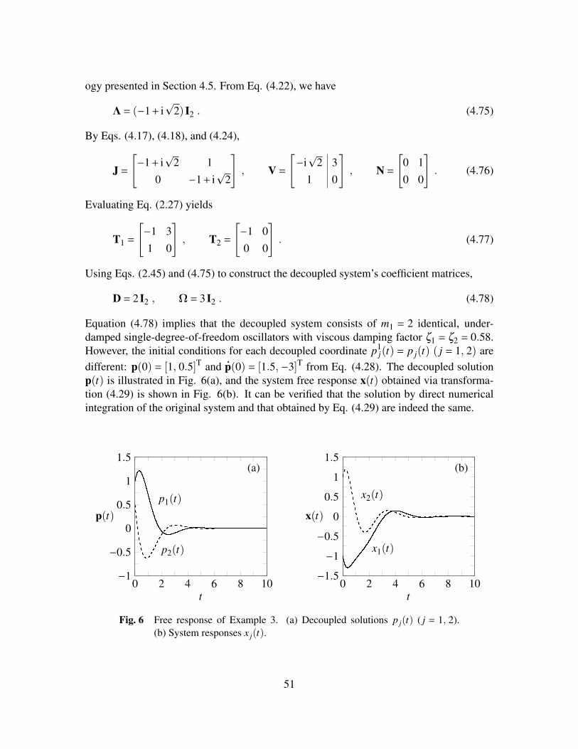
ogy presented in Section 4.5. From Eq. (4.22), we have

Λ= (−1+ ip

2) I2 . (4.75)

By Eqs. (4.17), (4.18), and (4.24),

J =[−1+ i

p2 1

0 −1+ ip

2

], V =

[−i

p2 3

1 0

], N =

[0 1

0 0

]. (4.76)

Evaluating Eq. (2.27) yields

T1 =[−1 3

1 0

], T2 =

[−1 0

0 0

]. (4.77)

Using Eqs. (2.45) and (4.75) to construct the decoupled system’s coefficient matrices,

D = 2 I2 , Ω= 3 I2 . (4.78)

Equation (4.78) implies that the decoupled system consists of m1 = 2 identical, under-damped single-degree-of-freedom oscillators with viscous damping factor ζ1 = ζ2 = 0.58.However, the initial conditions for each decoupled coordinate p1

j(t) = p j(t) ( j = 1, 2) aredifferent: p(0) = [1, 0.5]T and

.p(0) = [1.5, −3]T from Eq. (4.28). The decoupled solution

p(t) is illustrated in Fig. 6(a), and the system free response x(t) obtained via transforma-tion (4.29) is shown in Fig. 6(b). It can be verified that the solution by direct numericalintegration of the original system and that obtained by Eq. (4.29) are indeed the same.

0 2 4 6 8 10−1

−0.5

0

0.5

1

1.5

p1(t)

p2(t)

(a)

t

p(t)

0 2 4 6 8 10−1.5

−1

−0.5

0

0.5

1

1.5

x1(t)

x2(t)

(b)

t

x(t)

Fig. 6 Free response of Example 3. (a) Decoupled solutions p j(t) ( j = 1, 2).(b) System responses x j(t).

51

Example 4

Consider a non-classically damped, 2-degree-of-freedom system with mass matrix M=I2 and for which the damping matrix C and stiffness matrix K are given by

C =[

2 −1

−1 2

], K =

[1 −1

−1 2

]. (4.79)

Let the initial conditions be x(0) = [1, −1]T and.x(0) = [−2, −1]T. Solution of the associ-

ated quadratic eigenvalue problem reveals that the system possesses a single eigenvalue,a defective real eigenvalue λ1 = −1 with algebraic multiplicity m1 = 4 and unit geometricmultiplicity. The corresponding eigenvector v1

1 and generalized eigenvectors v1i (i= 2, 3, 4)

are

v11 =[

1

0

], v1

2 =[

1

1

], v1

3 =[

0

1

], v1

4 =[

1

−1

]. (4.80)

The sole eigenvector v11 has not been subjected to any normalization scheme. Since the al-

gebraic multiplicity of the single eigenvalue λ1 is even, we follow the decoupling procedurepresented in Section 4.6.2 with nr = 1. As m1 = 2, Eq. (4.46) yields

Λ= Λ=−I2 . (4.81)

By Eqs. (4.17), (4.18), and (4.47),

Jx =

−1 1 0 0

0 −1 1 0

0 0 −1 1

0 0 0 −1

, Vx =[

1 1 0 1

0 1 1 −1

], (4.82)

and it follows from Eqs. (4.50) and (4.51) that

Jp =

−1 1 0 0

0 −1 0 0

0 0 −1 1

0 0 0 −1

, Vp =[

1 0 0 0

0 0 1 0

]. (4.83)

From Eqs. (2.45) and (4.81), the coefficient matrices of the decoupled system are

D = 2 I2 , Ω= I2 . (4.84)

52

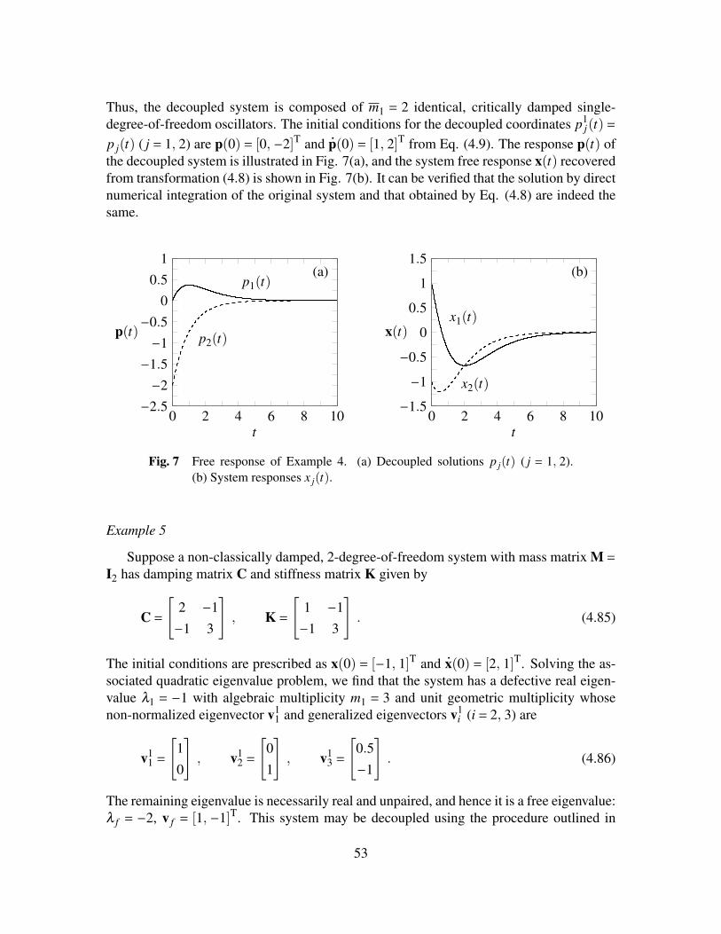
Thus, the decoupled system is composed of m1 = 2 identical, critically damped single-degree-of-freedom oscillators. The initial conditions for the decoupled coordinates p1

j(t)=p j(t) ( j = 1, 2) are p(0)= [0, −2]T and

.p(0)= [1, 2]T from Eq. (4.9). The response p(t) of

the decoupled system is illustrated in Fig. 7(a), and the system free response x(t) recoveredfrom transformation (4.8) is shown in Fig. 7(b). It can be verified that the solution by directnumerical integration of the original system and that obtained by Eq. (4.8) are indeed thesame.

0 2 4 6 8 10−2.5−2

−1.5−1

−0.50

0.51

p1(t)

p2(t)

(a)

t

p(t)

0 2 4 6 8 10−1.5

−1

−0.5

0

0.5

1

1.5

x1(t)

x2(t)

(b)

t

x(t)

Fig. 7 Free response of Example 4. (a) Decoupled solutions p j(t) ( j = 1, 2).(b) System responses x j(t).

Example 5

Suppose a non-classically damped, 2-degree-of-freedom system with mass matrix M =I2 has damping matrix C and stiffness matrix K given by

C =[

2 −1

−1 3

], K =

[1 −1

−1 3

]. (4.85)

The initial conditions are prescribed as x(0) = [−1, 1]T and.x(0) = [2, 1]T. Solving the as-

sociated quadratic eigenvalue problem, we find that the system has a defective real eigen-value λ1 = −1 with algebraic multiplicity m1 = 3 and unit geometric multiplicity whosenon-normalized eigenvector v1

1 and generalized eigenvectors v1i (i = 2, 3) are

v11 =[

1

0

], v1

2 =[

0

1

], v1

3 =[

0.5

−1

]. (4.86)

The remaining eigenvalue is necessarily real and unpaired, and hence it is a free eigenvalue:λ f = −2, v f = [1, −1]T. This system may be decoupled using the procedure outlined in

53

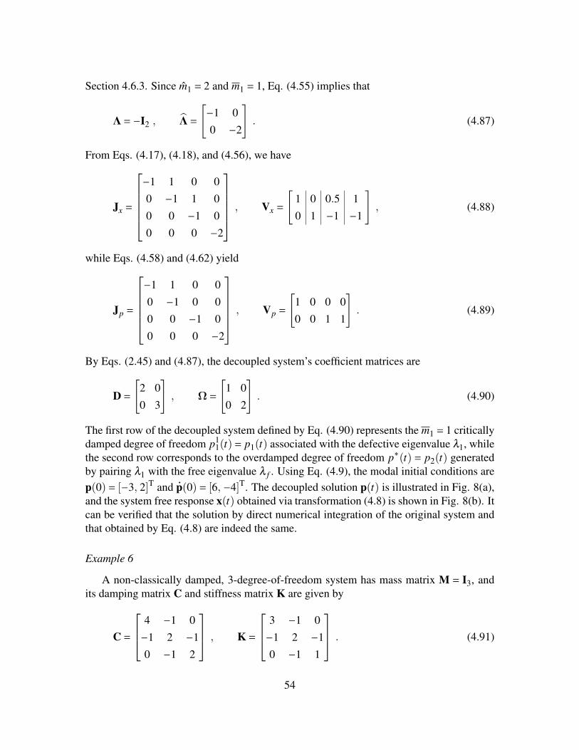
Section 4.6.3. Since m1 = 2 and m1 = 1, Eq. (4.55) implies that

Λ=−I2 , Λ=[−1 0

0 −2

]. (4.87)

From Eqs. (4.17), (4.18), and (4.56), we have

Jx =

−1 1 0 0

0 −1 1 0

0 0 −1 0

0 0 0 −2

, Vx =[

1 0 0.5 1

0 1 −1 −1

], (4.88)

while Eqs. (4.58) and (4.62) yield

Jp =

−1 1 0 0

0 −1 0 0

0 0 −1 0

0 0 0 −2

, Vp =[

1 0 0 0

0 0 1 1

]. (4.89)

By Eqs. (2.45) and (4.87), the decoupled system’s coefficient matrices are

D =[

2 0

0 3

], Ω=

[1 0

0 2

]. (4.90)

The first row of the decoupled system defined by Eq. (4.90) represents the m1 = 1 criticallydamped degree of freedom p1

1(t)= p1(t) associated with the defective eigenvalue λ1, whilethe second row corresponds to the overdamped degree of freedom p∗(t) = p2(t) generatedby pairing λ1 with the free eigenvalue λ f . Using Eq. (4.9), the modal initial conditions arep(0)= [−3, 2]T and

.p(0)= [6, −4]T. The decoupled solution p(t) is illustrated in Fig. 8(a),

and the system free response x(t) obtained via transformation (4.8) is shown in Fig. 8(b). Itcan be verified that the solution by direct numerical integration of the original system andthat obtained by Eq. (4.8) are indeed the same.

Example 6

A non-classically damped, 3-degree-of-freedom system has mass matrix M = I3, andits damping matrix C and stiffness matrix K are given by

C =

4 −1 0

−1 2 −1

0 −1 2

, K =

3 −1 0

−1 2 −1

0 −1 1

. (4.91)

54

0 2 4 6 8 10−3

−2

−1

0

1

2

p1(t)

p2(t)

(a)

t

p(t)

0 2 4 6 8 10−1.5

−1

−0.5

0

0.5

1

1.5

x1(t)

x2(t)

(b)

t

x(t)

Fig. 8 Free response of Example 5. (a) Decoupled solutions p j(t) ( j = 1, 2).(b) System responses x j(t).

Take as initial conditions x(0)= [1, 0, −1]T and.x(0)= [2, 1, 0]T. Solution of the associated

quadratic eigenvalue problem reveals that the system possesses a defective real eigenvalueλ1 = −1 with algebraic multiplicity m1 = 4 and geometric multiplicity ρ1 = 2. The corre-sponding eigenvectors v1

i (i = 1, 2) and generalized eigenvectors v1j ( j = 3, 4) are

v11 =

1

0

0

, v12 =

0

0

2

, v13 =

1

2

−2

, v14 =

0

−1

0

. (4.92)

The remaining eigenvalues are real and distinct:

λ2 =−3.41 , v2 =

1

−0.41

0.17

, λ3 =−0.59 , v3 =

0.17

0.41

1

. (4.93)

The eigenvectors v1i , v2, and v3 have not been subjected to any normalization scheme. To

decouple this system with mixed defective and non-defective real eigenvalues, the matricesJx, Vx, etc., will need to be constructed blockwise via direct sum using the matrix structures(4.10) and (4.11) at the end of Section 4.2 for non-defective eigenvalues and those presentedin Section 4.6 for defective real eigenvalues. However, while the algebraic multiplicity ofthe defective real eigenvalue λ1 is even, we may not employ the decoupling methodologyof Section 4.6.2 because λ1 has more than one associated eigenvector. Instead, proceedwith decoupling as follows. Pair the defective eigenvalue λ1 with corresponding eigen-vector v1

1 and, say, the distinct eigenvalue λ3 as real quadratic conjugates so as to yield anoverdamped degree of freedom. Of course, one may pair λ1 with λ2 instead, if preferred.

55

The remaining distinct eigenvalue λ2 necessarily becomes a free eigenvalue (i.e., λ f = λ2).Moreover, the Jordan chain for λ1 is of odd length m1 −1 = 3, and thus we may use theprocedure outlined in Section 4.6.3 to generate (m1 −2)/2 = 1 critically damped degree offreedom associated with λ1 and an overdamped degree of freedom by pairing λ1 with λ2.To implement this, use Eqs. (2.14) and (4.55) to construct

Λ=−I3 , Λ=

−1 0 0

0 −3.41 0

0 0 −0.59

. (4.94)

With the assistance of Eqs. (4.10) and (4.56),

Jx =

−1 1 0 0 0 0

0 −1 1 0 0 0

0 0 −1 0 0 0

0 0 0 −3.41 0 0

0 0 0 0 −1 0

0 0 0 0 0 −0.59

, (4.95)

Vx =

0 1 0 1 1 0.17

0 2 −1 −0.41 0 0.41

2 −2 0 0.17 0 1

. (4.96)

In addition, Eqs. (4.11), (4.58), and (4.62) imply that

Jp =

−1 1 0 0 0 0

0 −1 0 0 0 0

0 0 −1 0 0 0

0 0 0 −3.41 0 0

0 0 0 0 −1 0

0 0 0 0 0 −0.59

, (4.97)

Vp =

1 0 0 0 0 0

0 0 1 1 0 0

0 0 0 0 1 1

. (4.98)

56

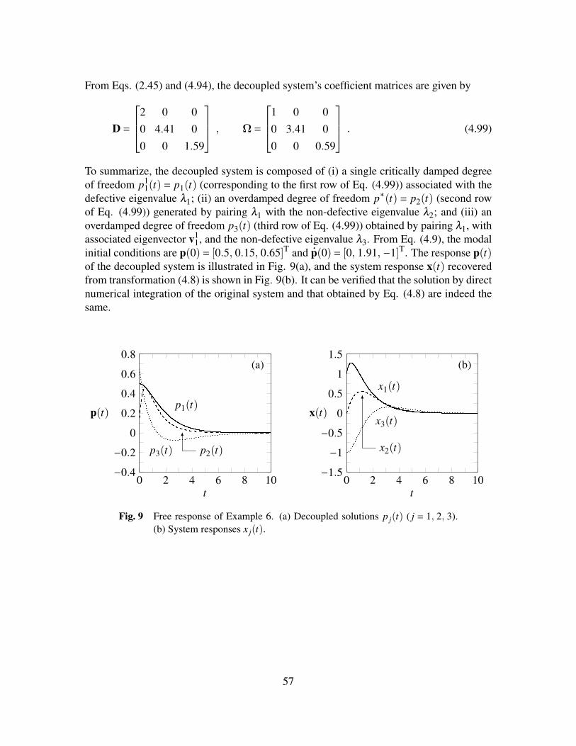
From Eqs. (2.45) and (4.94), the decoupled system’s coefficient matrices are given by

D =

2 0 0

0 4.41 0

0 0 1.59

, Ω=

1 0 0

0 3.41 0

0 0 0.59

. (4.99)

To summarize, the decoupled system is composed of (i) a single critically damped degreeof freedom p1

1(t) = p1(t) (corresponding to the first row of Eq. (4.99)) associated with thedefective eigenvalue λ1; (ii) an overdamped degree of freedom p∗(t) = p2(t) (second rowof Eq. (4.99)) generated by pairing λ1 with the non-defective eigenvalue λ2; and (iii) anoverdamped degree of freedom p3(t) (third row of Eq. (4.99)) obtained by pairing λ1, withassociated eigenvector v1

1, and the non-defective eigenvalue λ3. From Eq. (4.9), the modalinitial conditions are p(0)= [0.5, 0.15, 0.65]T and

.p(0)= [0, 1.91, −1]T. The response p(t)

of the decoupled system is illustrated in Fig. 9(a), and the system response x(t) recoveredfrom transformation (4.8) is shown in Fig. 9(b). It can be verified that the solution by directnumerical integration of the original system and that obtained by Eq. (4.8) are indeed thesame.

0 2 4 6 8 10−0.4

−0.2

0

0.2

0.4

0.6

0.8

p1(t)

p2(t)p3(t)

(a)

t

p(t)

0 2 4 6 8 10−1.5

−1

−0.5

0

0.5

1

1.5

x1(t)

x2(t)

x3(t)

(b)

t

x(t)

Fig. 9 Free response of Example 6. (a) Decoupled solutions p j(t) ( j = 1, 2, 3).(b) System responses x j(t).

57

Chapter 5Decoupling of Defective Systems inForced Motion

This chapter is concerned with (i) decoupling a forced defective system (1.1) into theform (1.2) and (ii) recovering the forced response x(t) exactly from the decoupled systemresponse p(t). We begin in Section 5.1 by developing a generalized decoupling transfor-mation in the state space that relates the decoupled solution p(t) to the response x(t) of anysystem of the type (1.1). The relationship between the applied excitation f(t) and the modalforcing g(t) is also established. We show in Section 5.2 that an explicit decoupling trans-formation exists in the configuration space when the eigenvalues are complex. The chaptercloses by illustrating in Section 5.3 how the methods presented here reduce to classicalmodal analysis if the coupled system (1.1) is classically damped.

5.1 A generalized state space representation

In general, the spectrum of a defective system (1.1) may contain any combination ofcomplex conjugate and real eigenvalues that are defective or not. With the assistance ofprevious work on forced non-defective systems and defective systems in free motion, de-coupling of forced vibration in this general setting is a fairly straightforward task. Beginby casting the equation of motion (1.1) in the first-order formulation[ .

x(t)..x(t)

]= A

[x(t).x(t)

]+[

OM−1

]f(t) , (5.1)

58

where the order 2n state matrix A is the same nonsymmetric matrix defined in Eq. (4.12).As before, we assume that the coefficient matrices D and Ω of the decoupled system (1.2)in free vibration remain unchanged upon application of an excitation f(t). Consequently,we define a generalized coordinate transformation for forced vibration based on the freeresponse’s time-dependent decoupling transformation (4.14):[

x(t).x(t)

]= Sx eJxt e−Jpt S−1

p

[p1(t)

p2(t)

]= S(t)

[p1(t)

p2(t)

]. (5.2)

It remains to be seen how the transformed coordinates p1(t) and p2(t) are related to theresponse p(t) of the decoupled system (1.2) and its corresponding velocity

.p(t). In the

usual manner, we next apply the coordinate transformation (5.2) to the first-order equation(5.1) and premultiply the resulting state equation by S−1(t), which gives[ .

p1(t).p2(t)

]= B

[p1(t)

p2(t)

]+S−1(t)

[O

M−1

]f(t)=

[O I−Ω −D

][p1(t)

p2(t)

]+[

g1(t)

g2(t)

], (5.3)

where the state matrix B is related to A by the time-varying transformation (4.16) and thetransformed excitations g1(t) and g2(t) are determined from[

g1(t)

g2(t)

]=[

Vp

Vp Jp

]eJpt e−Jxt

[Vx

Vx Jx

]−1[O

M−1

]f(t) . (5.4)

The upper and lower halves of state equation (5.3) are, respectively,

.p1(t)−p2(t)= g1(t) , (5.5)

.p2(t)+Dp2(t)+Ωp1(t)= g2(t) . (5.6)

By eliminating p2(t) from Eq. (5.6) using Eq. (5.5), we obtain

..p1(t)+D

.p1(t)+Ωp1(t)= Dg1(t)+

.g1(t)+g2(t) , (5.7)

which, by comparing it to system (1.2), implies that p1(t) can be identified with the decou-pled response p(t) and the modal excitation g(t) is given by

g(t)= Dg1(t)+.g1(t)+g2(t) . (5.8)

Lastly, setting p1(t) = p(t) in Eq. (5.5) and combining it with Eq. (5.2) yields the gen-eralized state space transformation that relates the decoupled solution p(t) to the system

59

response x(t) in forced vibration:[x(t).x(t)

]=[

Vx

Vx Jx

]eJxt e−Jpt

[Vp

Vp Jp

]−1[p(t)

.p(t)−g1(t)

]. (5.9)

The modal initial conditions p(0) and.p(0) are connected to the system initial conditions

x(0) and.x(0) by the state equation[

p(0).p(0)

]=[

Vp

Vp Jp

][Vx

Vx Jx

]−1[x(0).x(0)

]+[

0g1(0)

]. (5.10)

Thus, whether the eigenvalues of system (1.1) are defective or non-defective, complexor real, the system’s forced response x(t) may be recovered via transformation (5.9) uponsolution of the decoupled system (1.2) with excitation (5.8) and initial conditions (5.10).Differences between defective and non-defective systems and in how they are decoupledarise in the structures of the matrices Λ, Λ, Jx, Vx, Jp, and Vp, but the overall trans-formation in (5.9) is real regardless of the nature of the system’s spectrum. In principle,one could extract the upper half of the state equation (5.9) to obtain a time-dependent de-coupling transformation for x(t) itself in the n-dimensional configuration space, but thereis generally no concise analytical form. A flowchart outlining the general procedure fordecoupling any system of the form (1.1) and determining its response (free or forced) isillustrated in Fig. 10.

5.2 Complex eigenvalues

When the eigenvalues of system (1.1) are complex and defective, a decoupling trans-formation in the configuration space exists in a concise analytical form. By comparing thegeneralized decoupling transformation (5.9) for forced motion with its unforced counter-part (4.8), it is not difficult to see that one obtains state equation (5.9) by replacing themodal velocity p(t) in transformation (4.8) with

.p(t)−g1(t). Making this substitution in

Eq. (4.29) yields the configuration space transformation

x(t)= T1 eNt p(t)+T2 eNt .p(t)−T2 eNt g1(t) , (5.11)

where, with the aid of the time-dependent transformation S(t) in Eq. (4.31) and the stateequation (5.3), it is straightforward to show that[

g1(t)

g2(t)

]=[

e−Nt OO e−Nt

][I IΛ Λ

][V V

VJ VJ

]−1[O

M−1

]f(t) . (5.12)

60

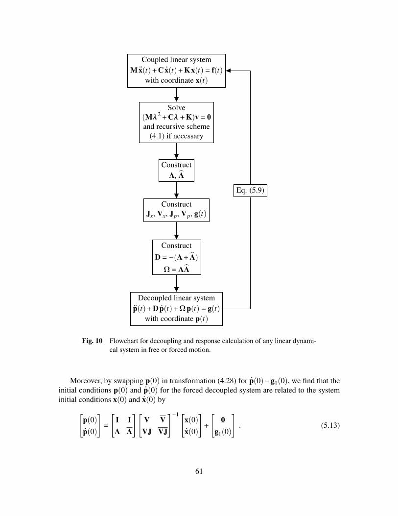
Coupled linear systemM

..x(t)+C

.x(t)+Kx(t)= f(t)

with coordinate x(t)

Solve(Mλ

2 +Cλ +K)v = 0and recursive scheme

(4.1) if necessary

ConstructΛ, Λ

ConstructJx, Vx, Jp, Vp, g(t)

Construct

D =−(Λ+ Λ)Ω=ΛΛ

Decoupled linear system..p(t)+D

.p(t)+Ωp(t)= g(t)

with coordinate p(t)

Eq. (5.9)

Fig. 10 Flowchart for decoupling and response calculation of any linear dynami-cal system in free or forced motion.

Moreover, by swapping p(0) in transformation (4.28) for.p(0)−g1(0), we find that the

initial conditions p(0) and.p(0) for the forced decoupled system are related to the system

initial conditions x(0) and.x(0) by[

p(0).p(0)

]=[

I IΛ Λ

][V VVJ VJ

]−1[x(0).x(0)

]+[

0g1(0)

]. (5.13)

61

In the event that the eigenvalues of system (1.1) are complex but non-defective, thenilpotent matrix N = O, and hence the Jordan matrix J = Λ. In this case, assuming theeigenvectors and their complex conjugates have been normalized in accordance with Eqs.(2.4) and (2.5), respectively, it can be shown that Eq. (5.12) for the excitations g1(t) andg2(t) simplifies to yield

g1(t)= TT2 f(t) , g2(t)= (TT

1 −DTT2 ) f(t) . (5.14)

As a result, the configuration space decoupling transformation (5.11) and modal forc-ing (5.8) reduce to the corresponding equations (3.10) and (3.7), respectively, for a non-defective system, as expected.

5.3 Reduction to classical modal analysis

Finally, we demonstrate how the decoupling transformation (5.9) is a direct generaliza-tion of classical modal analysis. Should system (1.1) be classically damped, the Jordan ma-trices Jx and Jp are identical because classical modal analysis preserves both the eigenval-ues and their multiplicities. Consequently, the time-dependent coordinate transformationS(t) in Eq. (5.2) reduces to the time-invariant form S(t) = S = Sx S−1

p . If the eigenvectorsare normalized according to Eqs. (2.42) and (2.43), then there is a certain pairing of thenon-defective real eigenvalues for which S = U⊕U, implying that the excitations g1(t)= 0and g2(t) = (MU)−1 f(t) = UT f(t) in Eq. (5.4). It follows that Eq. (5.8) yields the modalforcing g(t)= UT f(t) indicative of classical modal analysis. Furthermore, the upper half ofthe state equation (5.9) reduces to the classical modal transformation x(t)= Up(t). If nor-malizations (2.42) and (2.43) are not used, multiplicative constants may appear in certainequations.

5.4 An illustrative example

Here we provide a numerical example that demonstrates the decoupling procedure fora forced defective system of the type (1.1). We focus on a system with a non-defectivecomplex conjugate eigenvalue and a defective real eigenvalue to illustrate how one woulddecouple a defective system with mixed damping characteristics.

Example 7

Consider a non-classically damped, 2-degree-of-freedom system with mass matrix M=I2 and damping matrix C, stiffness matrix K, and excitation f(t) given by

C =[

2 −1

−1 2

], K =

[1 −1

−1 3

], f(t)=

[0.2 cost

−0.7sint

]. (5.15)

62

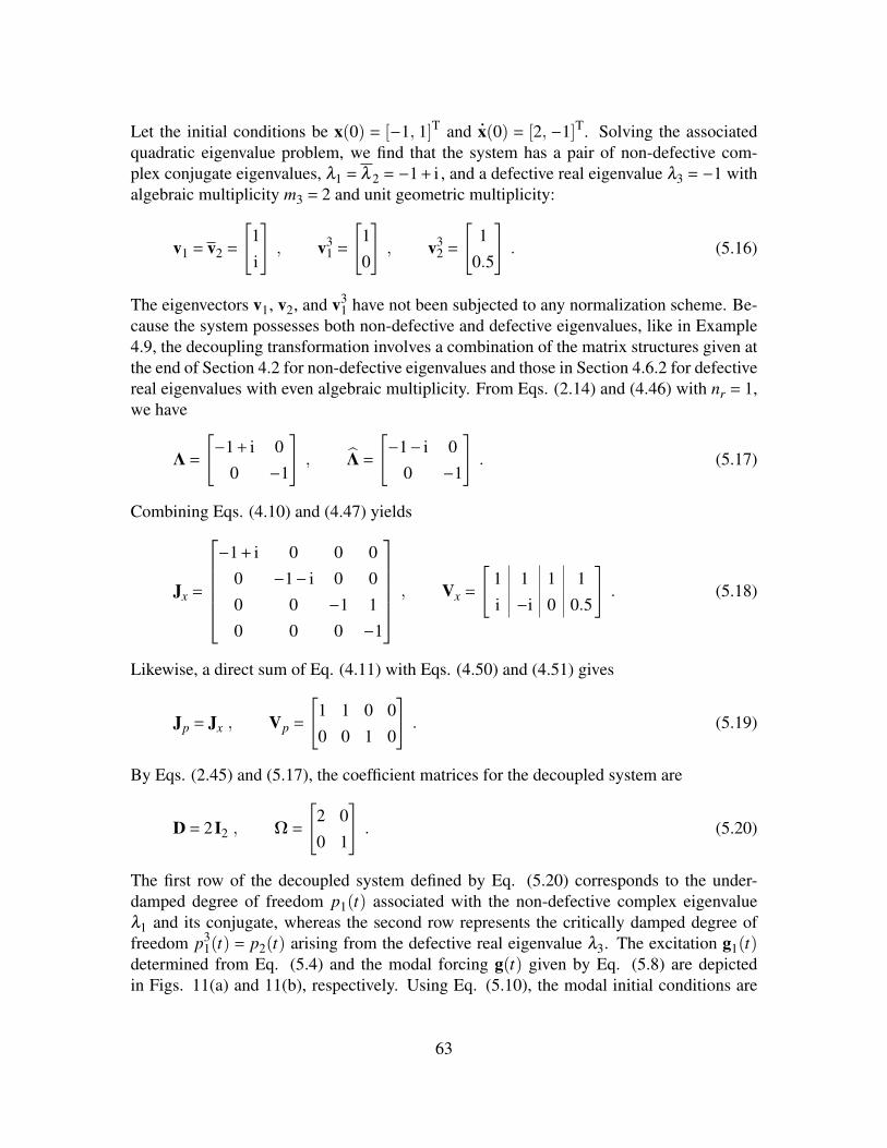
Let the initial conditions be x(0) = [−1, 1]T and.x(0) = [2, −1]T. Solving the associated

quadratic eigenvalue problem, we find that the system has a pair of non-defective com-plex conjugate eigenvalues, λ1 = λ 2 =−1+ i , and a defective real eigenvalue λ3 =−1 withalgebraic multiplicity m3 = 2 and unit geometric multiplicity:

v1 = v2 =[

1

i

], v3

1 =[

1

0

], v3

2 =[

1

0.5

]. (5.16)

The eigenvectors v1, v2, and v31 have not been subjected to any normalization scheme. Be-

cause the system possesses both non-defective and defective eigenvalues, like in Example4.9, the decoupling transformation involves a combination of the matrix structures given atthe end of Section 4.2 for non-defective eigenvalues and those in Section 4.6.2 for defectivereal eigenvalues with even algebraic multiplicity. From Eqs. (2.14) and (4.46) with nr = 1,we have

Λ=[−1+ i 0

0 −1

], Λ=

[−1− i 0

0 −1

]. (5.17)

Combining Eqs. (4.10) and (4.47) yields

Jx =

−1+ i 0 0 0

0 −1− i 0 0

0 0 −1 1

0 0 0 −1

, Vx =[

1 1 1 1

i −i 0 0.5

]. (5.18)

Likewise, a direct sum of Eq. (4.11) with Eqs. (4.50) and (4.51) gives

Jp = Jx , Vp =[

1 1 0 0

0 0 1 0

]. (5.19)

By Eqs. (2.45) and (5.17), the coefficient matrices for the decoupled system are

D = 2 I2 , Ω=[

2 0

0 1

]. (5.20)

The first row of the decoupled system defined by Eq. (5.20) corresponds to the under-damped degree of freedom p1(t) associated with the non-defective complex eigenvalueλ1 and its conjugate, whereas the second row represents the critically damped degree offreedom p3

1(t) = p2(t) arising from the defective real eigenvalue λ3. The excitation g1(t)determined from Eq. (5.4) and the modal forcing g(t) given by Eq. (5.8) are depictedin Figs. 11(a) and 11(b), respectively. Using Eq. (5.10), the modal initial conditions are

63

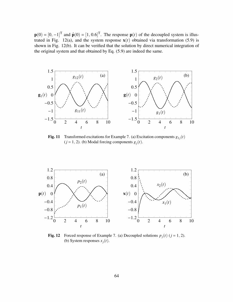
p(0) = [0, −1]T and.p(0) = [1, 0.6]T. The response p(t) of the decoupled system is illus-

trated in Fig. 12(a), and the system response x(t) obtained via transformation (5.9) isshown in Fig. 12(b). It can be verified that the solution by direct numerical integration ofthe original system and that obtained by Eq. (5.9) are indeed the same.

0 2 4 6 8 10−1.5

−1

−0.5

0

0.5

1

1.5

g11(t)

g12(t) (a)

t

g1(t)

0 2 4 6 8 10−1.5

−1

−0.5

0

0.5

1

1.5

g1(t)

g2(t)(b)

t

g(t)

Fig. 11 Transformed excitations for Example 7. (a) Excitation components g1 j(t)( j = 1, 2). (b) Modal forcing components g j(t).

0 2 4 6 8 10−1.2

−0.8

−0.4

0

0.4

0.8

1.2

p1(t)

p2(t)

(a)

t

p(t)

0 2 4 6 8 10−1.2

−0.8

−0.4

0

0.4

0.8

1.2

x1(t)

x2(t)

(b)

t

x(t)

Fig. 12 Forced response of Example 7. (a) Decoupled solutions p j(t) ( j = 1, 2).(b) System responses x j(t).

64

Chapter 6Closing Comments

We have demonstrated how classical modal analysis may be extended to decouple anysecond-order linear dynamical system (1.1). By formulating a decoupling transformationin a general framework, a complete solution to the problem of decoupling linear dynam-ical systems, defective or not, in free or forced motion has been provided. Major resultspresented in this dissertation are summarized in the following statements:

1. Any non-defective system can be decoupled via phase synchronization, which gen-erates a real, nonlinear, and time-dependent decoupling transformation in both theconfiguration and state spaces that preserves the system eigenvalues and their multi-plicities. In the case of free vibration, the decoupling transformation becomes linearand time-shifting in the configuration space, while it reduces to a linear but time-invariant transformation in the state space.

2. Non-defective complex conjugate eigenvalues are associated with underdamped de-grees of freedom. Pairing of non-defective real eigenvalues as real quadratic conju-gates generates overdamped degrees of freedom. Non-uniqueness in pairing the realeigenvalues results in a set of admissible decoupled systems.

3. Any system with defective eigenvalues can be decoupled if one does not insist onpreserving geometric multiplicities. In contrast with non-defective systems, the de-coupling transformation for defective systems in free vibration is time-dependent inboth the configuration and state spaces.

65

4. Associated with defective complex conjugate eigenvalues are underdamped degreesof freedom. Defective real eigenvalues correspond to critical damping. Dependingon the multiplicities of these eigenvalues, decoupling yields some combination ofcritically damped degrees of freedom and overdamped degrees of freedom, the latterresulting from a necessary pairing of either defective and non-defective eigenvalues,or two distinct defective eigenvalues.

5. All parameters required for generating the decoupled system (1.2) and evaluatingthe general decoupling transformation (5.9) are obtained by solving the quadraticeigenvalue problem (2.1), determining generalized eigenvectors from the recursivescheme (4.1) when eigenvalues are defective, and applying an admissible eigenvaluepairing scheme as described herein.

6. Decoupling transformation (5.9) is a direct generalization of classical modal analysis.

As system decoupling plays a fundamental role in linear vibratory analysis, it is ourhope that the information presented in this dissertation will facilitate numerical and qual-itative analyses of linear dynamical systems, as well as inspire both theorists and practi-tioners to pursue further research in oft-slighted, but mathematically fascinating, defectivesystems.

66

References

[1] L. Meirovitch, Analytical Methods in Vibrations, Macmillan, New York, 1967.

[2] H. Benaroya, Mechanical Vibration: Analysis, Uncertainties, and Control, PrenticeHall, Upper Saddle River, 1998.

[3] L. Meirovitch, Fundamentals of Vibrations, International ed., McGraw Hill, NewYork, 2001.

[4] J. W. Strutt (Lord Rayleigh), The Theory of Sound, Vol. I, Macmillan, London, 1877.

[5] T. K. Caughey, M. E. J. O’Kelly, “Classical normal modes in damped linear dynamicsystems,” ASME Journal of Applied Mechanics 32 (1965) 583–588.

[6] R. W. Clough, S. Mojtahedi, “Earthquake response analysis considering non-proportional damping,” Earthquake Engineering and Structural Dynamics 4 (1976)489–496. doi:10.1002/eqe.4290040506.

[7] H.-C. Tsai, J. M. Kelly, “Non-classical damping in dynamic analysis of base-isolatedstructures with internal equipment,” Earthquake Engineering and Structural Dynam-ics 16 (1988) 29–43. doi:10.1002/eqe.4290160104.

[8] H.-C. Tsai, J. M. Kelly, “Seismic response of the superstructure and attached equip-ment in a base-isolated building,” Earthquake Engineering and Structural Dynamics18 (1989) 551–564. doi:10.1002/eqe.4290180409.

[9] A. K. Chopra, Dynamics of Structures: Theory and Applications to Earthquake Engi-neering, 3rd ed., Prentice Hall, Upper Saddle River, 2007.

[10] R. A. Frazer, W. J. Duncan, A. R. Collar, Elementary Matrices, 2nd ed., CambridgeUniversity Press, New York, 1955.

[11] K. A. Foss, “Co-ordinates which uncouple the equations of motion of damped lineardynamic systems,” ASME Journal of Applied Mechanics 25 (1958) 361–364.

67

[12] A. S. Veletsos, C. E. Ventura, “Modal analysis of non-classically damped linearsystems,” Earthquake Engineering and Structural Dynamics 14 (1986) 217–243.doi:10.1002/eqe.4290140205.

[13] G. Prater Jr., R. Singh, “Quantification of the extent of non-proportional viscousdamping in discrete vibratory systems,” Journal of Sound and Vibration 104 (1)(1986) 109–125. doi:10.1016/S0022-460X(86)80134-1.

[14] S. S. Nair, R. Singh, “Examination of the validity of proportional damping approxi-mations with two further numerical indices,” Journal of Sound and Vibration 104 (2)(1986) 348–350. doi:10.1016/0022-460X(86)90274-9.

[15] J. Bellos, D. J. Inman, “Frequency response of nonproportionally damped, lumpedparameter, linear dynamic systems,” ASME Journal of Vibration and Acoustics 112(1990) 194–201. doi:10.1115/1.2930112.

[16] I. W. Park, J. S. Kim, F. Ma, “Characteristics of modal coupling in nonclassicallydamped systems under harmonic excitation,” ASME Journal of Applied Mechanics61 (1994) 77–83. doi:10.1115/1.2901425.

[17] M. Tong, Z. Liang, G. C. Lee, “An index of damping non-proportionality for discretevibrating systems,” Journal of Sound and Vibration 174 (1) (1994) 37–55. doi:

10.1006/jsvi.1994.1554.

[18] A. Bhaskar, “Estimates of errors in the frequency response of non-classically dampedsystems,” Journal of Sound and Vibration 184 (1) (1995) 59–72. doi:10.1006/

jsvi.1995.0304.

[19] A. Bhaskar, “Mode shapes during asynchronous motion and non-proportionality in-dices,” Journal of Sound and Vibration 224 (1) (1999) 1–16. doi:10.1006/jsvi.

1997.1070.

[20] K. Liu, M. R. Kujath, W. Zheng, “Identification of non-proportionality of dampingin discrete vibratory systems,” Computers and Structures 77 (2000) 557–569. doi:

10.1016/S0045-7949(99)00230-8.

[21] U. Prells, M. I. Friswell, “A measure of non-proportional damping,” Mechanical Sys-tems and Signal Processing 14 (2) (2000) 125–137. doi:10.1006/mssp.1999.

1280.

[22] K. Liu, M. R. Kujath, W. Zheng, “Evaluation of damping non-proportionality us-ing identified modal information,” Mechanical Systems and Signal Processing 15 (1)(2001) 227–242. doi:10.1006/mssp.2000.1326.

[23] S. Adhikari, “Optimal complex modes and an index of damping non-proportionality,”Mechanical Systems and Signal Processing 18 (2004) 1–27. doi:10.1016/

S0888-3270(03)00048-7.

68

[24] M. Morzfeld, N. Ajavakom, F. Ma, “Diagonal dominance of damping and the decou-pling approximation in linear vibratory systems,” Journal of Sound and Vibration 320(2009) 406–420. doi:10.1016/j.jsv.2008.07.025.

[25] J. K. Knowles, “On the approximation of damped linear dynamical systems,” Struc-tural Control and Health Monitoring 13 (2006) 324–335. doi:10.1002/stc.130.

[26] W. T. Thomson, T. Calkins, P. Caravani, “A numerical study of damping,” Earth-quake Engineering and Structural Dynamics 3 (1974) 97–103. doi:10.1002/eqe.

4290030108.

[27] D. L. Cronin, “Approximation for determining harmonically excited response of non-classically damped systems,” ASME Journal of Engineering for Industry 98 (1976)43–47.

[28] S. M. Shahruz, F. Ma, “Approximate decoupling of the equations of motion of linearunderdamped systems,” ASME Journal of Applied Mechanics 55 (1988) 716–720.doi:10.1115/1.3125855.

[29] S. F. Felszeghy, “On uncoupling and solving the equations of motion of vibratinglinear discrete systems,” ASME Journal of Applied Mechanics 60 (1993) 456–462.doi:10.1115/1.2900815.

[30] J. Angeles, S. Ostrovskaya, “The proportional-damping matrix of arbitrarily dampedlinear mechanical systems,” ASME Journal of Applied Mechanics 69 (2002) 649–656.doi:10.1115/1.1483832.

[31] T. K. Hasselman, “Modal coupling in lightly damped structures,” AIAA Journal14 (11) (1976) 1627–1628. doi:10.2514/3.7259.

[32] S. M. Shahruz, A. K. Packard, “Large errors in approximate decoupling of nonclas-sically damped linear second-order systems under harmonic excitations,” Dynamicsand Control 4 (1994) 169–183. doi:10.1007/BF01985940.

[33] A. Ibrahimbegovic, E. L. Wilson, “Simple numerical algorithms for the mode su-perposition analysis of linear structural systems with non-proportional damping,”Computers and Structures 33 (2) (1989) 523–531. doi:10.1016/0045-7949(89)

90026-6.

[34] F. E. Udwadia, R. S. Esfandiaria, “Nonclassicaly damped dynamic systems: An it-erative approach,” ASME Journal of Applied Mechanics 57 (1990) 423–433. doi:

10.1115/1.2892007.

[35] J. H. Hwang, F. Ma, “On the approximate solution of nonclassically damped linearsystems,” ASME Journal of Applied Mechanics 60 (1993) 695–701. doi:10.1115/

1.2900860.

69

[36] F. E. Udwadia, R. Kumar, “Iterative methods for non-classically damped dynamicsystems,” Earthquake Engineering and Structural Dynamics 23 (1994) 137–152.doi:10.1002/eqe.4290230203.

[37] S. D. Garvey, M. I. Friswell, U. Prells, “Co-ordinate transformations for second ordersystems, part I: General transformations,” Journal of Sound and Vibration 258 (5)(2002) 885–909. doi:10.1006/jsvi.2002.5165.

[38] S. D. Garvey, M. I. Friswell, U. Prells, “Co-ordinate transformations for second ordersystems, part II: Elementary structure-preserving transformations,” Journal of Soundand Vibration 258 (5) (2002) 911–930. doi:10.1006/jsvi.2002.5166.

[39] M. T. Chu, N. Del Buono, “Total decoupling of general quadratic pencils, part I:Theory,” Journal of Sound and Vibration 309 (2008) 96–111. doi:10.1016/j.jsv.2007.05.058.

[40] M. T. Chu, N. Del Buono, “Total decoupling of general quadratic pencils, part II:Structure preserving isospectral flows,” Journal of Sound and Vibration 309 (2008)112–128. doi:10.1016/j.jsv.2007.05.052.

[41] P. Lancaster, L. Rodman, “Canonical forms for Hermitian matrix pairs under strictequivalence and congruence,” SIAM Review 47 (3) (2005) 407–443. doi:10.1137/S003614450444556X.

[42] P. Lancaster, I. Zaballa, “Diagonalizable quadratic eigenvalue problems,” Mechani-cal Systems and Signal Processing 23 (2009) 1134–1144. doi:10.1016/j.ymssp.

2008.11.007.

[43] U. Prells, M. I. Friswell, “A relationship between defective systems and unit-rankmodification of classical damping,” ASME Journal of Vibration and Acoustics 122(2000) 180–183. doi:10.1115/1.568458.

[44] M. I. Friswell, U. Prells, S. D. Garvey, “Low-rank damping modifications and defec-tive systems,” Journal of Sound and Vibration 279 (2005) 757–774. doi:10.1016/

j.jsv.2003.11.042.

[45] F. Ma, A. Imam, M. Morzfeld, “The decoupling of damped linear systems in oscil-latory free vibration,” Journal of Sound and Vibration 324 (2009) 408–428. doi:

10.1016/j.jsv.2009.02.005.

[46] F. Ma, M. Morzfeld, A. Imam, “The decoupling of damped linear systems in freeor forced vibration,” Journal of Sound and Vibration 329 (2010) 3182–3202. doi:

10.1016/j.jsv.2010.02.017.

[47] M. Morzfeld, F. Ma, “The decoupling of damped linear systems in configuration andstate spaces,” Journal of Sound and Vibration 330 (2011) 155–161. doi:10.1016/

j.jsv.2010.09.005.

70

[48] P. Lancaster, Lambda-Matrices and Vibrating Systems, Pergamon Press, Oxford,1966.

[49] I. Gohberg, P. Lancaster, L. Rodman, Matrix Polynomials, Academic Press, NewYork, 1982.

[50] F. Tisseur, K. Meerbergen, “The quadratic eigenvalue problem,” SIAM Review 43 (2)(2001) 235–286. doi:10.1137/S0036144500381988.

[51] A. Sestieri, S. R. Ibrahim, “Analysis of errors and approximations in the use of modalco-ordinates,” Journal of Sound and Vibration 177 (2) (1994) 145–157. doi:10.

1006/jsvi.1994.1424.

[52] L. Meirovitch, Principles and Techniques of Vibrations, Prentice Hall, Upper SaddleRiver, 1997.

[53] I. Stakgold, Green’s Functions and Boundary Value Problems, 2nd ed., John Wiley &Sons, Hoboken, 1998.

[54] D. Rowell, D. N. Wormley, System Dynamics: An Introduction, Prentice Hall, UpperSaddle River, 1997.

[55] G. H. Golub, C. F. Van Loan, Matrix Computations, 3rd ed., The John Hopkins Uni-versity Press, Baltimore, 1996.

[56] J. W. Demmel, Applied Numerical Linear Algebra, SIAM, Philadelphia, 1997.

[57] E. Anderson, Z. Bai, C. Bischof, S. Blackford, J. Demmel, J. Dongarra, J. Du Croz,A. Greenbaum, S. Hammarling, A. McKenney, D. Sorensen, LAPACK Users’ Guide,3rd ed., SIAM, Philadelphia, 1999.

[58] U. Prells, P. Lancaster, “Isospectral vibrating systems, part 2: Structure preservingtransformations,” Operator Theory: Advances and Applications 163 (2005) 275–298.doi:10.1007/3-7643-7516-7_12.

[59] D. E. Beskos, B. A. Boley, “Critical damping in linear discrete dynamic systems,”ASME Journal of Applied Mechanics 47 (1980) 627–630. doi:10.1115/1.3153744.

[60] D. J. Inman, A. N. Andry Jr., “Some results on the nature of eigenvalues of discretedamped linear systems,” ASME Journal of Applied Mechanics 47 (1980) 927–930.doi:10.1115/1.3153815.

[61] J. A. Gray, A. N. Andry Jr., “A simple calculation for the critical damping matrix ofa linear multidegree of freedom system,” Mechanics Research Communications 9 (6)(1982) 379–380.

71

[62] A. Bhaskar, “Criticality of damping in multi-degree-of-freedom systems,” ASMEJournal of Applied Mechanics 64 (1997) 387–393. doi:10.1115/1.2787320.

[63] R. M. Bulatovic, “On the critical damping in multi-degree-of-freedom sys-tems,” Mechanics Research Communications 29 (2002) 315–319. doi:10.1016/

S0093-6413(02)00263-X.

[64] S. Papargyri-Beskou, D. E. Beskos, “On critical viscous damping determination inlinear discrete dynamic systems,” Acta Mechanica 153 (2002) 33–45. doi:10.1007/BF01177049.

[65] B. H. Tongue, Principles of Vibration, 2nd ed., Oxford University Press, New York,2001.

72