Monthly Variability in the Ocean Habitat off Peru as Deduced from Maritime Observations, 1953 to 1984 ANDREW BAKUN PacificFisheries EnvironmentalGroup Southwest Fisheries Center National Marine Fisheries Service, NOAA P.O. Box 831, Monterey California 93942, USA BAKUN, A. 1987. Monthly variabiihy ntz ocean habitat off Peru as deduced from maritime objervations,1953 to 1984, p. 46-74. In D. Pauly and I. Tsukayama (eds.) The Peruvian anchoveta and its upwelling ecosystem: three decades of change. ICLARM Studies and Reviews 15, 351 p. Instituto del Mar del Peru (IMARPE), Callao, Peru; Deutsche Geselischaft fir Technische Zusammenarbeit (GZ), GinbH, Eschbom, Federal Republic of Germany; and International Center for Living Aquatic Resources Management (ICLARM), Manila, Philippines. Abstract Monthly time series, generated from summaries of maritime reports from fhe region off Peru, are presented for the period 1953 to 1984. These include sea surface temperature, cloud cover, atmospheric pressure, "wind-cubed" index of rate of addition of turbulent mixing energy to the ocean by the wind, wind stress components, solar radiation, long-wave back radiation, evaporative heat loss and net atmosphere-ocean heat exchange. All series are found to undergo interrelated nonseasonal variations at multiyear periods. El Nffo episodes ae characterized by intense turbulent mixing of the ocean by the wind, intense offshore-directed Ekman transport and by low net heat gain to the ocean through the sea surface. Effects of constant versus variable transfer coefficient formulations on the bulk aerodynamic flux estimates are discussed. Certain comments on the utilization of these data in analysis of biological effects arc offered. Introduction By international convention, weather observations are recorded routinely on a various types of ships operating at sea. These maritime reports remain the primary source of information on large-scale variability in the marine environment. Even with the increasing development of satellite observation systems, analysis of time series of decadal length and longer must continue' to depend heavily on these maritime reports for some time to come. Observations of wind speed and direction, air and sea temperature, atmospheric pressure, humidity and cloud cover included in these reports provide a basis for estimating a number of environmental variables pertinent to the study of variations in ocean climate and of effects of these variations on the associated communities of marine organisms. In this paper, the historical files of these C ;ervations are summarized to yield monthly estimates of properties and processes at the sea surface within the extremely productive upwelling ecosystem off central and northern Peru. The 32-year period treated encompasses several dramatic El Nifio events and the spectacular rise, collapse, and indications of a recent rebound, of the largest exploited fish population that has ever existed, the Peruvian anchoveta. Although remarkably rich both in biological productivity and in climatic scale ocean variability, the area off Peru is rather poor in maritime data density. Thus the region presents a particular challenge to the methodologies emnployed here. The area is very sparsely sampled in comparison to the con'esponding eastern ocean boundary ecosystems of the northern hemisphere, with most of the reports coming from a narrow coastal shipping lane lying within about 200 km of the coast (Parrish et al. 1983). Maritime reports are subject to a variety of measurement and transmission errors, of which improper positioning is perhaps the most troublesome, sometimes introducing very large errors in all derived quantities (e.g., when a wrong hemisphere, etc., may 46

Welcome message from author
This document is posted to help you gain knowledge. Please leave a comment to let me know what you think about it! Share it to your friends and learn new things together.
Transcript
Monthly Variability in the Ocean Habitat off Peru
as Deduced from Maritime Observations 1953 to 1984
ANDREW BAKUN PacificFisheriesEnvironmentalGroup
Southwest FisheriesCenter NationalMarineFisheriesServiceNOAA
POBox 831 Monterey California93942 USA
BAKUN A 1987 Monthly variabiihy ntz ocean habitat off Peru as deduced from maritime objervations1953 to 1984 p 46-74 In D Paulyand I Tsukayama (eds) The Peruvian anchoveta and its upwelling ecosystem three decades of change ICLARM Studies andReviews 15 351 p Instituto del Mar del Peru (IMARPE) Callao Peru Deutsche Geselischaft fir Technische Zusammenarbeit(GZ) GinbH Eschbom Federal Republic of Germany and International Center for Living Aquatic Resources Management(ICLARM) Manila Philippines
Abstract Monthly time series generated from summaries of maritime reports from fhe region off Peru are presented for the period 1953 to 1984These include sea surface temperature cloud cover atmospheric pressure wind-cubed index of rate of addition of turbulent mixing energy tothe ocean by the wind wind stress components solar radiation long-wave back radiation evaporative heat loss and net atmosphere-ocean heatexchange All series are found to undergo interrelated nonseasonal variations at multiyear periods El Nffo episodes ae characterized by intenseturbulent mixing of the ocean by the wind intense offshore-directed Ekman transport and by low net heat gain to the ocean through the seasurface Effects of constant versus variable transfer coefficient formulations on the bulk aerodynamic flux estimates are discussed Certaincomments on the utilization of these data in analysis of biological effects arc offered
Introduction
By international convention weather observations are recorded routinely on a various typesof ships operating at sea These maritime reports remain the primary source of information onlarge-scale variability in the marine environment Even with the increasing development ofsatellite observation systems analysis of time series of decadal length and longer must continueto depend heavily on these maritime reports for some time to come Observations of wind speedand direction air and sea temperature atmospheric pressure humidity and cloud cover includedin these reports provide a basis for estimating a number of environmental variables pertinent tothe study of variations in ocean climate and of effects of these variations on the associatedcommunities of marine organisms In this paper the historical files of these C ervations aresummarized to yield monthly estimates of properties and processes at the sea surface within theextremely productive upwelling ecosystem off central and northern Peru The 32-year periodtreated encompasses several dramatic El Nifio events and the spectacular rise collapse andindications of a recent rebound of the largest exploited fish population that has ever existed thePeruvian anchoveta
Although remarkably rich both in biological productivity and in climatic scale oceanvariability the area off Peru is rather poor in maritime data density Thus the region presents aparticular challenge to the methodologies emnployed here The area is very sparsely sampled incomparison to the conesponding eastern ocean boundary ecosystems of the northern hemispherewith most of the reports coming from a narrow coastal shipping lane lying within about 200 kmof the coast (Parrish et al 1983) Maritime reports are subject to a variety of measurement andtransmission errors of which improper positioning is perhaps the most troublesome sometimesintroducing very large errors in all derived quantities (eg when a wrong hemisphere etc may
46
47
be indicated) And it is difficult to establish effective procedures for rejecting erroneous reportswithout also suppressing indications of real variations particularly in the area off Peru which is perhaps uniquely subject to drastic and abrupt natural environmental perturbations For example early indications of the 1982-1983 El Niio event went unnoticed by meteorological agencies in Europe and North America because the reports which clearly indicated an event of unprecedented intensity were so far from the norm that they are rejected as erroneous by the automated data editing procedures (Siegel 1983) In addition even when no actual errors are involved irregular distribution of the reports in both time and space may introduce biases and nonhomogeneities into time series constructed from these data
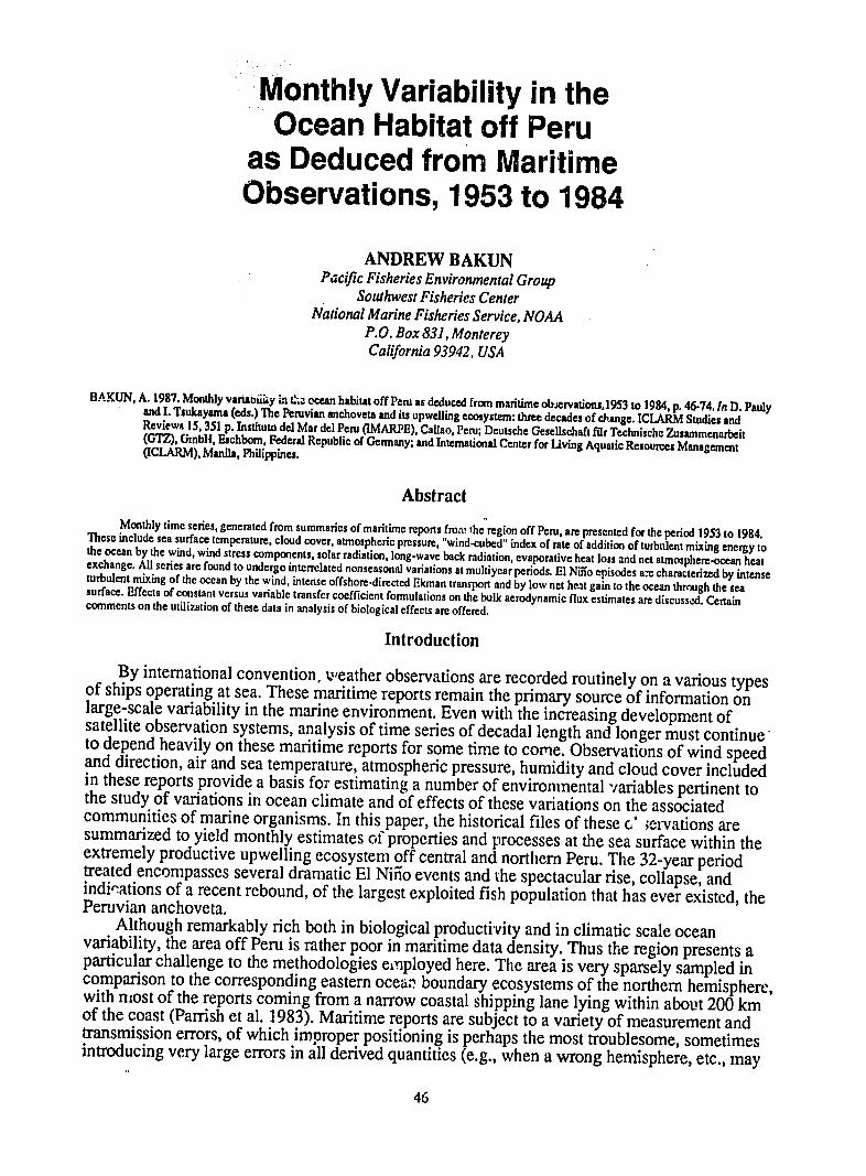
Tests of the precision of the methodology on interyear time scales involving subsamplings of the much richer data distributions off the Iberian Peninsula in the northeast Atlantic Oceanhave indicated benefits to be gained by utilizing rather large areal samples ie of the order of 10 degrees of latitude and longitude in extent with the increase in report frequency overridingincreases in sampling variance resulting from incorporation of additional spatial variability (Bakun unpublished data) These same tests have indicated that the use of the ordinary standard error of the mean provides a useful guide to the precision of monthly estimates even though the underlying processes may be very highly variable on much smaller temporal and spatial scales than those used for data summarization For the time series presented herein reports available within an area extending some 10 degrees of latitude along the Peru coast and about 4 degrees of longitude offshore (Fig 1) between Talara and a point just to the south of Pisco were
los
Tlara
Chimbote
10oS
M Cullao )U
15S -Ju
200S 1 1 1 1 1 I850W 80-W 75 700 W
Fig 1 Summary area Maritime reports from within the area indicated by diagonal hatching were uIsad foraIssIembli n ontihly samnples
48
composited together These composite samples are assumed to characterize temporal variabilityat least in the relative sense in conditions affecting the neritic fish habitat along that stretch ofcoastline which appears to have some degree of natural unity both in terms of environmentalprocesses and biological community (Santander 1980 Parrish et al 1983) The rather raggedoffshore edge of the summary region was chosen to facilitate initial extraction of the reportsfrom the data archive files Consistent features of spatial variability tend to be much less intensein offshore areas of coastal upwelling regions than in coastal areas thus no substantial effect ofthe irregularity of shape of the offshore boundary is expected Also all the monthly summaries are treated identically in terms of areal selection and so time series homogeneity is preserved Inany case report density is extremely low at the outer edge of the summary area
Assembly of Data Series
Impossible or highly improbable values occur occasionally in the maritime report files dueto keypunch errors etc In the data record format temperature values between -999 and 9990C are possible Initial efforts to construct the data series resulted in rather large standard errors forcertain of the monthly values due to incorporation of improbable data For this reason onlyvalues falling between the limits 11 to 31oC were accepted as valid observations of airtemperature sea surface temperature or wet bulb air temperature for this region (Note that thelower bound on the wet bulb temperature caused only 16 reports no more than a single report inany one month to be rejected) Wind speeds of up to 199 knots (102 msec) are possible in therecord format Erroneously high wind speeds have a particularly serious effect since wind speedis squared in the stress computation and cubed in the wind mixing index formulation Reports ofwind greater than 45 knots (23 msec) occurred within the summary region less than ten times inthe entire 32-year record and were in no case corroborated by neighboring (in either space ortime) data Thus wind reports exceeding this value were excluded in preparing these time seriesThe data record format limited wind direction to values between 0 and 360 degrees cloud coverobservations to the range 0 to 100 of sky obscured and barometric pressure to values between890 and 1070 millibars
In assembling the monthly data samples if any one of the reported values of sea surfacetemperature barometric pressure wind speed or wind direction were missing or unacceptablethe entire report was excluded from the summaries These four observed properties are sufficientto produce time series of sea surface temperature (Table 2) atmospheric pressure (Table 4) windstress components (Tables 5 and 6) and wind mixing index (Table 7) The numbers of reportshaving acceptable observations of these four items are entered as the first of the three numbersshown for each month in Table 1 In addition if a valid cloud cover observation was availablethe report was also incorporated in the cloud cover series (Table 3) numbers of reports includingacceptable observations of these five items are entered as the second number of each monthly setin Table 1Finally if acceptable values of both air (dry bulb) temperature and either wet bulb ordew point temperature were included the report was also used for construction of time series oftmosphere-ocean heat exchange components (Tables 8 to 11) Numbers of available reportscontaining acceptable observations of all seven properties required to construct all the time seriespresented in this paper are shown as the third number under each month in Table 1Allcomputations of derived quantities were performed on each individual report prior to anysummarization process A simple mean was taken as an estimate of the central tendency of eachmonthly sample Computed standard errors of these mean values are displayed within theparentheses following each monthly value presented in the various data tables An approximate95 confidence interval estimate can thus be generated by multiplying the indicated standarderror by the factor 196 and adding and subtracting the result from the monthly mean value(point estimate) to yield the upper and lower limits of the intervalA small percentage of the reports contain wind observations in which the direction is notedas variable ie no direction could be assigned This properly occurs only when the windspeed is very low In these cases the wind speed is used as reported in the calculations where itenters as a scalar quantity ie in the calculations of wind mixing index evaporative heat lossand conductive heat loss In the computation of surface wind stress wind enters as a vector
49
quantity and directionality is crucial Accordingly for the surface wind stress calculationsvariable winds are treated as calms Because the wind speed enters the calculation as a squarelow wind values act essential as zeros in their effect on the monthly means and so treating theseweak variable wind observations as calms has no substantial effect Also the net effect of a stress from one direction is cancelled by an equal stress from the opposite direction and so treating variable-directional stress as equivalent to calm conditions makes physical sense
Sea Surface Wind Stress
Sea surface stress was estimated according to
(ry)= pa CD ( lNto 1Uio 1 101o V10) 1)
where Tx and ryare components of stress directed onshore and alongshore respectively acharacte-istic onshore direction of 62 degrees and an alongshore direction of 332 degrees (fromtrue north) was assigned to the entire summary area Pa is the density of air considered constant at 122 kgm3 CD is a dimensionless drag coefficient 1W10 1 is the wind speed at 10 m heightU10 is the onshore-directed component of wind velocity V10 is the alongshore-directed(positive equatorward) component For the data series presented in the tables CD wasconsidered to be a constant equal to 00013 The use of this constant drag coefficient has been a somewhat standard practice in climatological studies of upwelling regions (Bakun et al 1974Nelson 1977 Parrish et al 1983) However it is recognized that the value of the drag coefficient is actually a variable which depends on the nature of atmospheric turbulence near the seasurface Thus a dependence on both atmospheric stability and wind magnitude near the seasurface is indicated the stability effect is particularly important in reducing air-sea transfers inupwelling regions due to the stable atmospheric boundary layer formed over cool upwelledsurface water No clear consensus as to he proper formulation of these dependencies is presentlyavailable However a reasonable variable drag coefficient formulation has been chosen and hasbeen applied to these data for evaluation of possible differences from results based on the constant drag coefficient formulation In this case we follow the method of Nelson (1977) forincorporation of the atmospheric stability effect which is based on a bulk Richardson number parameterization (Deardorff 1968) We incorporate a dependence on wind speed according to therecommendations of Large and Pond (1981) who find a linear increase in the drag coefficient atwind speeds greater than 11 Imsec
Offshore Ekman Transport
In their climatological study of seasonality and geography of anchovy and sardinereproductive habitats within eastern ocean boundary upwelling systems Parrish et al (1983)found a pattern of minimization of both wind-driven offshore surface flow (Ekman transport)and of wind-induced turbulence in the spawning habits of these fishes They therefore suggestthe likelihood of important effects of both processes on reproductive success Offshore Ekman transport at a given latitude is proportional to the alongshore stress being simply the product ofthe alongshore stress and the reciprocal of the local Coriolis parameter Ekman transport (Ekman1905) provides an acceptable description of ocean surface transport directly driven by surface wind stress at periods which are long compared to the half-pendulum day the half-pendulum dayis 29 actual days in length at 100 latitude but increases to infinity at the equator Obviously theEkman transport description cannot be applied directly at the equator Here we assume theEkman transport description to be adequate for the effect of wind stress variations affecting the summary area as a whole on the monthly time scale thus we simply divide the monthlyalongshore wind stress by a characteristic value of the Coriolis parameter (we choose the localvalue at IOOS ie 00000253sec to characterize offshore Ekman transport in response to largeshyscale long period wind variations over the anchoveta reproductive habitat this choice will affect
so
the average magnitude but not the time series properties of the resulting indicator series which will be identical to those of the alongshore stress series)
Wind Mixing Index
The rate at which the wind imparts mechanical energy to the ocean to produce turbulentmixing of the upper water column is roughly proportional to the third power or cube of thewind speed (Elsberry and Garwood 1978) A wind mixing index which is simply the mean ofthe cube of the observed wind speeds in each monthly sample (Table 7) is presented as a guide tolonger period variability in this particular process However it is to be noted that these series may not reflect energetic shbrter-term variability which may b- more crucial to reproductivesuccess of anchovies (Husby and Nelson 1982) The hypothetical basis for interest in this processin relation to anchoveta reproductive success is Laskers (1978) suggestion that first-feedingsuccess of anchovy larvae may be dependent upon availability of fine scale food particleconcentrations which may be dispersed by wind-driven turbulent mixing events These occur atatmospheric storm event scales which are much shorter than one month Furthermore it is notthe exact magnitude of mixing that is crucial according to this hypothesis but rather theexistence of time-space survival windows within which the rate of addition of turbulence bythe wind does not reach a level that homogenizes the food particle distributions (Bakun andParrish 1980) The wind speed level at which this occurs and the minimum required duration ofthe window for substantial survival to result are unclear and undoubtedly are variable functionsof other factors such as water column stability the particular food particle organisms growthrate behavior motility etc In any case the maritime reports occur irregularly in time and spaceand so are no amenable to indicating durations of periods characterized by specific conditionseven if we were able to specify the required nature of the conditions This would requireutilization of a time-and-space continuous meteorological analysis procedure (Bakun 1986)which might be ineffective due to the low maritime report density in the region and particularlyseaward of the region The use cf shore station data despite interference from local topographicinfluences etc might be the best available option for indicating short time scale wind ariabilityover the ocean habitat off Peru (see Mendo et al this vol)
Solar Radiation
Net incominampsolar radiation QS absorbed by the ocean was estimated according to the formula
QS= ( - a) Qo (I - 062C + 00019h) 2)
where ot is the fraction of incoming radiation reflected from the sea surface Q0 is the sum of thedirect and diffuse radiation reaching the ground under a cloudless sky C is the observed totalcloud amount in tenths of sky covered and h is the noon solar altitude For each maritime reportthe total daily direct solar radiation reaching the ground under cloudless conditions was extractedfrom the Smithsonian Meteorological Tables (List 1949) as a function of the date and latitude ofthe report using a 4 x 4 element curvilinear interpolation on the table entries via Bessels centraldifference formida and assuming the atmospheric transmission coefficient of 07 rezommendedby Seckel and Beaudry (1973) The diffuse solar radiation was estimated according to Listsrecommendations as follows The solar radiation reaching the top of the atmosphere was extracted from the appropriate table This value was decreased by 9 to allow for water vaporabsorption and 2 for ozone absorption The result is subtracted from the value previouslydetermined for the direct radiation reaching the ground to yield the energy scattered out of thesolar beam This is reduced by 50 (to reflect the fact that half is diffused upward and thereforeonly half is diffused downward) to yield the total diffuse solar radiation reaching the ground Thetotal daily direct and diffuse radiation values corresponding to each report are then summed to
51
yield QS The remainder of the computation follows the procedures adopted by Nelson andHusby (1983) The linear cloud correction in Equation (2) is as suggested by Reed (1977) andReeds recommendation that no correction be made for cloud amounts less than 025 of total sky was followed Sea surface albedo was extracted from Paynes (1972) tables following Nelsonand Husbys (1983) algorithm which consists of entering the tables with the 07 atmospherictransmission coefficient rcduced by a factor equal to the linear cloud correction applied inEquation (2) and the mean daily solar altitude The possible error in the net radiation estimateintroduced by using the mean daily solar altitude to indicate albedo rather than an integration over the entire day of entries at short time intervals with instantaneous solar altitudes is estimated to be of the order of 1
Radiative Heat Loss
Effective back radiation is the difference between the outgoing long-wave radiation from the sea surface which depends on the 4th power of the absolute temperature of the sea surface andthe incoming long-wave radiation from the sky which depends on the water vapor content of theatmosphere and on the nature of the cloud cover Here we follow exactly the computationalscheme of Nelson and Husby (1983) who used the modified Brunt equation (Brunt 1932) withthe empirical constants of Budyko (1956) and the linear cloud correction formula of Reed (1976)to compute the effective back radiation (radiative heat loss) QB
-QB = 550 x 10 1 (Ts + 27316) 4 (039- 005ea2)(1 - 09C) 3)
The vapor pressure of the air ea was computed according to the formula provided in the Smithsonian Meteorological Tables (List 1949) using the observed barometric pressure and drybulb and wet bulb air temperatures For reports that were without an acceptable wet bulb temperature but included an acceptable dew point temperature the vapor pressure was computed as the saturation vapor pressure at the dew point temperature using an integrated form of the Clausius-Clapeyron equation (Murray 1967)
Evaporative and Conductive Heat Losses
In estimating evaporative heat loss (latent heat transfer) and conductive heat loss (sensibleheat transfer) the procedures of Nelson and Husby (1983) are again followed closely except for a modification of the wind speed dependence in their variable transfer coefficient formulations as indicated below The bulk aerodynamic formula for turbulent fluxes of latent and sensibleheat across the air-sea interface in a neutrally stable atmospheric boundary layer (Kraus 1972) can be expressed as
QE = Pa LC E(qo - q 1o) 1W10 I 4)
Q =PaCPCH (T3 - Ta) W I 5)
where and I1 are as in Equation (1) with Paassigned the same constant value (122 kgm3) asin the stress computation L is the latent heat of vaporization assigned a constant value of 245 x106 J)kg (5853 calgm) cp is the specific heat of air assigned a constant value of 1000 JkgOC(0239 calgoc) The empirical exchange coefficients CE and CH were assigned constantvalues of 00013 in the construction of the time series presented in Tables 10 and 11 n additiontime series based on variable transfer coefficient formulations incorporating dependencies on atmospheric stability and on wind speed were also assembled for comparison These formulations are again those chosen by Nelson and Husby (1983) which incorporate the
52
atmospheric stability effect according to a bulk Richardson number parameterization (Deardorff1968) however Nelson and Husbys wind speed dependencies were in this case modifiedaccording to the recommendations of Large and Pond (1982) who suggest an increase in CE andCH which is proportional to the square root of the wind speed The specific humidities of the airin contact with the sea surface qO and at 10 m or deck level qi0 were computed according to e
q E-e6)P
where E is the known ratio (a constant equal to 0622) of the molecular weight of water vapor tothe net molecular weight of dry air e is the vapor pressure and P is the barometic pressure Forthis calculation the variation in P is negligible and so a constant value of 101325 pascals(101325 mb) was assigned The calculation of eat 10 m or deck level is as indicated for theradiative heat loss calculation (Equation 3) To calculate e at the sea surface the saturation vaporpressure over pure water was computed from a formula given by Murray (1967) and reduced by2 to account for the effect of salinity (Miyake 1952)
SJ24 A- 350oD
2 300a
lU20 150 U cntn0mM
t 182Ssm 0 50 U)16 -- IJ 9LJL
J F M A M J J A S 0 N D J F M A M J J A S 0 N D
i [M alongshore component
BE 1 onshore component 1_ 1 07shy
1013shy 20esoal-vr0n-LFS 04
-11012-03
0 COL 101 J F M A M J J A S 0 N D 00 ddAS
C F []seasonal ly- varying MLD
12o80 constant 20m MVLD
- o6 shy
04
02 0 5
Ftg 2 Seasonal cycles 32-yr mean monthly values
53
The Seasonal Cycles
The idea of regular seasonal cycles for the coupled ocean-atmosphere system off Peru is to some degree illusory in view of the predominint influence of interyear variability in the regionHowever the seasonal variation is the most cyclic and predictable of the large components of variability It is therefore the conponent of variation which is most likely to be reflected in biological adaptations Accordiz gly a summary of the long-term mean monthly values of the various series (Figs 2 and 3) sen es as a useful starting point for discussion
Being situated within the tropical band the region experiences two passages of the sun each year the sun is directly overhead in October and again in February-March Also since the earths meteorological equator is displaced to the north of the geographical equator the region is dominated by southern hemisphere atmospheric dynamics thus austral winter dominates the seasonality of transfers of momentum and mechanical energy from atmosphere to ocean
The 32-year mean monthly sea surface temperature (Fig 2A) is at a maximum in March coinciding with the second period of vertical sun which marks the culmination of the extended austral summer period of relatively high sun The temperature falls to a minimum in August The atmospheric pressure (Fig 2B) tends to be directly out of phase being at a minimum in the austral summer and at a maximum in the winter season Cloudiness (Fig 2C) lags the atmospheric pressure variation by about one month On average less than 50 of the sky is obscured by clouds in April this increases to greater than 85 in September
The strength of the wind exhibits a typical southern hemisphere seasonality being strongestin austral winter and weakest in summer Thus the 32-year mean monthly values of the index of rate of addition of turbulent mixing energy to the water column (Fig 2D) reach a maximum in August-September and a minimum in January The fact that the seasonal spawning peak of anchoveta is centered within this August-September turbulent mixing maximum would indicate non-adaptation of reproductive strategy for minimization of turbulent mixing effects This is not in accordance with the general pattern suggested by Parrish et al (1983) as generallycharacterizing seasonality and geography of spawning of eastern ocean boundary anchovypopulations Although no claim is made for conclusiveness the inference would seem to be that Laskers (1978) hypothesis is not at least in most years the major factor affecting anchoveta reproductive success off Peru Note that the level of turbulent mixing index intensity off Peru is low compared to other anchovy reproductive habitats even at its seasonal maximum
The alongshore component of wind stress on the sea surface is consistently equatorward in no case in the 32-year series (Table 5) did any monthly wind mean stress value deviate from this predominently alongshore and equatorward tendency in the transfer of momentum from atmosphere to ocean The long-term mean values of alongshore stress (Fig 2E) follow the same seasonal pattern as the turbulent mixing index reaching a maximum in September and a minimum in January The 32-year mean monthly values of the onshore component of stress are small compared to those of the alongshore component but are positive (onshore-directed) at all seasons
Surface Ekman transport being proportional to the alongshore stress but directed perpendicularly to the left of the stress is thus directed offshore with a seasonal maximum againcorresponding to the seasonal spawning peak of anchoveta This anomaly to the pattern of apparent minimization of offshore transport in spawning strategies of engraulids puzzled Bakun and Parrish (1982) However Parrish et al (1983) showed that the seasonal variation in mixed layer depth off Peru proceeds in phase with that of transport in response to the seasonalities in turbulent mixing (Fig 2C) and surface cooling (Fig 2A) but has greater relative amplitude The result is that drifting organisms which are distributed through the upper mixed layer would experience a faster net offshore drift in the thinner surface mixed layer of austral summer than in the deeper mixed layer of winter even though the winter transport (by volume) is much largerThis is illustrated in Fig 2F which shows calculations of mean monthly offshore Ekman velocity of the mixed layer performed in two different ways (based on the 32-year mean monthlyvalues of the data presented in Table 5) Firstly the monthly estimates of offshore Ekman transport are divided by the composite mean (20 m) of the mixed layer depth values given for 2shymonth segments of the seasonal cycle by Parrish et al (1983) Secondly the same monthlyestimates of offshore Ekman transport are divided by monthly mixed layer depth estimates
54
produced by curvilinear interpolation of the 2-month seasonal segments The effect of variable mixed layer depth on the net offshore velocity is apparent and suggestive of adaptation of spawning seasonality for avoidance of offshore loss of larvae (for additional discussion of this aspect see Bakun 1985) The effect of the choice of a constant or variable drag coefficient formulation in the stress computation (Equation 1)on the seasonal signal is indicated in Fig 3AThe 32-year mean monthly Ekman transport values based on the variable coefficient formulation follow a seasonal progression which is very similar to those based on the constant coefficient formulation (ie presented in Table 5) however they are slightly smaller in magnitudereflecting the effect of stability in the atmospheric boundary layer which is stabilized as theonshore-directed airflow is cooled from below while traversing the coastal upwelling zone
Solar radiation entering the ocean (Qs) is at a maximum during the February overhead passage of the sun (Fig 3B) This is due to substantially reduced cloud cover relative to the November solar passage Solar radiation is at a minimum in July when solar altitude has justpassed its June minimum and cloudiness is approaching its winter maximum
30 A constant coeft 6 D 30 m variable coeff E25constant coeff 25 0variable coeff
20
15 E
-10gt
05 10
00 WJ F M A M J J A S 0ON D J F M A M J J A S 0 N D
B250 M constant coef f M variable coeff
0150 04
25100
2 50 5
0 0
C F M A M J J A S O N D J F M A M J J A S O N D
CY~ constant coeff 30-200variable coefV
0154lu
C
Fig 3 Seasonal cycles 32-yr mean monthly values (Note that the SI-standard heat flux units watts per square meter may be converted to calories per square centimeter per day by multiplying by the factor 2604)
55
Heat loss from the sea surface via long-wave radiation (QB) is only a small fraction of theshort-wave radiation absorbed reflecting the areas location within the tropical band (Fig 3C)Radiative heat loss is at a seasonal maximum during April corresponding to the minimum incloudiness and at a minimum in September corresponding to the cloudiness maximum
Heat loss from the ocean via evaporation at the sea surface (QE) is at a maximum duringaustral winter and at a minimum during summer (Fig 3D) The choice of constant or variabletransfer coefficient has only a slight effect with the results of the variable coefficientformulation appearing to increase very slightly in magnitude relative to those of the constant coefficient formulation toward the summer and fall seasons
Heat loss via conduction (Qc) is very small compared to the other heat exchangecomponents (Fig 3) This is fortunate because the choice of transfer coefficient formulationcompletely changes the seasonal pattern With the constant coefficient formulation conductiveheat loss is mostly negative indicating heating of the ocean surface by contact with theatmosphere This reflects the common situation of cool upwelling-affected surface waters beingin contact with a generally warmer atmosphere However the strong stability of the atmosphereboundary layer inherent in this situation inhibits conductive heat transfer according to thevariable transfer coefficient formulation Thus the less common situation where the air is coolerthan the water dominates the sensible heat transfer according to the variable coefficentformulation with the result that conductive heat loss is indicated as being positive in all the 32shyyear composite monthly means except the summer months of January and February
The 32-year monthly means of the time series of atmosphere-ocean heat exchange (QN)which represent the resultant differences between the amount of solar radiation absorbed by the ocean and the sum of the heat losses due to long-wave radiation evaporation and conductionindicate substantial heat gain by the ocean throughout the year (Fig 3F) As expected the average heatgain is greatest in austral summer reaching values of the order of 200 wattsm2(413 cal cm-2 day-1) in January and least in winter falling to about 70 wattsm 2 (144 cal cm-2 day-i) in July The constant coefficient formulations yield slightly greater numerical values ofnet heat exchange than do the variable coefficient formulations mainly due to the differences inthe respective indications of the conductive heat loss component discussed in the previousparagraph however the respective seasonal progressions are very similar
Interyear Variations
If cyclical seasonal effects are those most likely to be adapted for and incorporated in lifecycle strategies of organisms major nonseasonal variations are those most likely to causedisruptions in life cycle processes and therefore to be reflected in population variations Veryshort-scale nonseasonal variations are not well resolved in these monthly composites ofirregularly distributed maritime reports However when shorter period variability is smoothedand the cyclic seasonal effects are suppressed nonseasonal variations of longer than annualperiod which -represent substantial perturbations of the environmental normalcy to whichreproductive strategies or other life cycle strategies should have become tuned are clearlymanifested For the purposes of this discussion a simple 12-month running mean filter is chosen to suppress sea sonalities and smooth the higher frequencies
Problems (negative side lobes wavelength-dependent phase shifts etc) with such equallyshyweighted moving average filters are well known (Anon 1966) However in this case thealternatives also present problems We particularly wish to suppress the seasonal cycle and soweighting the filter elements to suppress side lobes at other frequencies while increasing leakageof the seasonal frequency is not desirable Smoothed monthly series of anomalies from longshyterm monthly means (eg Quinn et al 1978 McLain et al 1985) have the property that thefiltering is nonlocal ie that any value is dependent on other values in the same calendarmonth in temporally distant parts of the time series Thus for example an intense warming(eg El Niiio) occurring within a generally cool climatic period appears as a much less intenseanomaly than a warming of similar magnitude within a warm period also the degree ofindicated intensity changes whenever the length of the series used for determination of the longshyterm mean changes More importantly if the amplitude (or shape phase etc) of the seasonal
56
variation is undergoing nonseasonal variation taking anomalies introduces spurious seasonalshyscale variations into the filtered series A local seasonal filter that avoids some of these problems can be based on 12th-differences eg the result of subtracting from each monthlyvalue the value for the same calendar month in the previous year but the result is therebytransformed to annual rates of change of a property rather than the property itself which complicates a descriptive discussion However the use of 12th-difference transforms is worth considering for empirical modelling efforts For the purposes of this discussion the simple 12shymonth running mean provides a local seasonal filtersmoother which will be familiar to manyreaders and adequate for a descriptive treatment
The filtered sea surface temperature series (Fig 4A) illustrates well the major El Niio warm events of the period 1957-1958 1965 1969 1972-1973 1976 and 1982-1983 Generallyelevated temperatures in the period between the 1976 and 1983 events are also apparent Also apparent is the extended cold period of the mid- 1950s the indication of rise in temperature from this cold period to the peak of the 1957-1983 El Niiio is comparable in total magnitude to that of the rise of the 1982-83 El Ni-io from the much warmer climatic base temperature level of the late 1970s
Major features in the filtered cloud cover series (Fig 4B) are visibly related to those in the temperature series but not in any simple consistent manner Cloud cover minima often appearto coincide with the relaxation of El Nifio events An extraordinarily low degree of cloudings appears to have coincided with the return to normal sea temperatures in 1984 Another sharpcloud cover minimum coincided with the leveling off of the temperature decline following the 1957-1958 event Likewise cloud cover maxima often appear to coincide with rapid drops of temperature into cool periods Atmospheric pressure variations (Fig 4C) are obviously highlyinversely correlated at these low frequencies with those of sea surface temperature
It is not surprising in view of the dynamic linkage of wind to horizontal gradient of atmospheric pressure that wind variations would be related to those of atmospheric pressureThe relation of the wind-cubed index of rate of addition of turbulent mixing energy to the ocean by the wind (Fig 4D) to El Nifio periods is striking El Niffo events are evidently strongwind-mixing events which according to Laskers (1978) scenario would correspond to periodsof high probability of starvation for first-feeding anchoveta larvae The period during and immediately following the 1972 El Nifio appears to have been characterized by an extended period of highly turbulent upper water column conditions The period during and following the 1982-1983 event appears to have been similarly turbulent except for a 2-month window of relaxed turbulent mixing index during December 1983 and January 1984 (somewhat masked bythe smoothing in Fig 4C but evident in the unsmoothed monthly values in Table 7)
The magnitude of alongshore (equatorward) wind stress also increases during El Nifio events (Fig 4E) in agreement with Wyrtkis (1975) conclusions which were based on a summary area displaced somewhat southward along the coast (10-200S 70-80oW) from the oneused here (Fig 1) Thus in addition to potential increases in larval starvation due to increased destruction of food particle strata by turbulent mixing an increase in potential offshore loss of larvae from the favorable coastal habitat is also indicated The onshore component of surface wind stress is relatively small and consistently positive (onshore-directed) in the filtered series
In the previous section the effect of seasonally-varying mixed layer depth on the offshore Ekman velocity of particles which are continually mixed through the upper mixed layer was discussed (ie in reference to Fig 2F) To investigate the effect on interyear time scales filtered time series of offshore Ekman velocity were calculated as in that section ie (i) assuming a constant MLD of 20 m and (ii) assuming a seasonally varying MLD derived from the values given by Parrish et al (1983) The result indicates that at least for the MLD values chosen the effect of seasonally-varying mixed layer depth is such as to substantially increase on average the rate of offshore movement of passive particles in the mixed layer If the effective mixed layerdepth is increased during El Nifio as would be expected both from the effect of the propagatingbaroclinic wave in deepening the surface layer and also from the enhanced wind induced turbulent mixing the effect would be to counteract the increased rate of offshore movement indicated from the Ekman transport calculations
The effect of the choice of constant or variable drag coefficient formulation in the stress computation (Equation 1)is illustrated in Fig 4G where the alongshore stress variation is
25 S24- 28
V)
21
is-1_
55
20
is-__var
60 65
Year
70 75 80
85
020-
---
-1612
-- shy
55
60 65
Year
70
tp
constant coefficientviable coefficient
75 80
-
85
B H
1220 -
- -681 oW210
60
55
56
60 65 Yea
70 75
80
)
85
2 20
u ~190 55 60 65
Year 70
75
80 s
-
85
10135-
13
E10120shy
30
10125-a
010o 55 60 65
Year 70 75 80 85
22
Year
Fig 4 Low-frquency nonseasonal variations 12-month running means of monthly time series values (Note that the SI-standard heat flux units watts per square meter may be converted to calories per square centimeter per day by multiplying by the factor 2064)
-t-4
Ln
D
iso- 80constant 70
coefficientshyvariable coefficient
200
040
B-30 -20shy
55 60 65 Y aYear 80 85 55 60 65 Ya 70 75 80 85
E K
5
Eon~shor
C- 2
tol_
lonshore com ponent copnn --
ID
ISO
160
is 140
12D
I
I00
constant coefficient -
variable coefficient
-
55 60 65 70 75
YeauirY e a r
80 85
~ ~iii~
55 60 65 70
Year -Y 008
75 85
mnl mean lnaitude
2ee e pe ue c pe d by mliyn h factor52064)81b
- seasonally-varying MID ----- e 795 55
6 -
60 0
65 775 80 85 55 60 1 IIl5 I
65 7075 08 Y e ar YYore a -
Fig 4 Continued Low-frequency nonseasonal varitions 12-month running -neans of monthly time series values (Note that the Sl-standard heat flux units watts per square meter may be converted to calories per square centimeter perday by multiplying by the factor 2064)
59
plotted in terms of its directly proportional transform offshore Ekman transport The variable coefficient formulation produces generally lower estimates of stress due to the influence of the stability of the lower atmospheric boundary layer over upwelling-affected surface waters However the differences essentially disappear during the period of relaxation of the intense El Niios of 1957-1958 and 1982-1983 A possible explanation is the tendency for a less stable atmosphere in contact with the ocean surface due to residual warmth which would linger longerin the ocean than in the atmosphere due to the much greater heat storage capacity of water compared to that of air
The filtered series of estimates of absorption of solar radiation by the ocean (QS) exhibits some interesting patterns (Fig 4H) Since the variables that control the solar radiation estimate (Equation 2) derived from a maritime report at any given latitude are calendar date and cloud cover it is not surprising that maxima in Fig 4H often correspond to minima in Fig 4B and vice versa However there are discernible differences between the two series that result from the interaction of the cloud cover variations with the seasonal changes in solar height in the solar radiation time series An impressive feature in the solar radiation series is the early largeshyamplitude alternation consisting of deep minimum of solar radiation entering the ocean corresponding to the early part of the intense 1954-1955 cold period followed by a sharp highlyerratic rise to a high peak in early 1960 In addition the entire period of the 1960s and the first half of the 1970s appears to have been characterized by low absorption of solar radiation relative to the more recent period since 1976
The long-wave radiative heat loss (QB) tends to be an order of magnitude smaller than the short-wave absorption but varies very similarly (Fig 41) This similarity is perhaps explainablein the similar dependence of both types of estimate on cloud cover with the sea surface temperature dependence in the long-wave radiation estimate (Equation 3) being related seasonally to the solar height dependence in the solar radiation estimate (Equation 2) There mayalso be some actual causal effect of the long period variations in solar radiation on the sea temperature dependence in the long-wave radiation estimate
The filtered series of evaporative heat loss (QE) delineates the various El Niffo episodes and the 1954-1955 cold period in a very similar fashion to the sea surface temperature series (Fig4J) The long-term variation in vapor pressure difference between the sea surface and the overlying atmosphere (Equation 4) is apparently very closely linked to that of sea surface temperature As discussed above the wind speed dependence is also a strong function of these climate scale events The effect of choice of constant or variable transfer coefficient apparentlymakes very little difference except during the mid-1950s cold period where increased stability of the air over the cold ocean apparently inhibited the turbulent exchange of latent heat according to the variable coefficient formulation
The net ocean-atmosphere heat exchange series (QN) indicates long-term variations in net ocean heat gain such that minima are associated with El Nifio episodes and maxima with cold periods The variations appear to be controlled to a substantial extent by the evaporative heat loss (Fig 4J) This is so because the variations in heat gain by absorption of short-wave solar radiation (Fig4H) are partially offset by the highly correlated variations in long-wave radiative heat loss (Fig 41) The net effect of the choice of variable or constant transfer coefficient formulations in the evaporative and conductive components is a slight general lowering of the magnitude oi net heat gain in the variable coefficient case This difference is due primarily to the stability effect on the conductive heat loss term as discussed in the previous section in reference to Fig 2E where the average change in the mean net value of this component approximately 5 wattsm2 corresponds in general to the approximate difference between the curves in Fig 4K except in the mid-1950s where stability effects on the evaporative heat loss term are appreciable
In order to check for long-period variations in the distribution of observations within the summary area (Fig 1) filtered series of the monthly averages of the respective latitudinal and longitudinal locations of reports were prepared (Fig 4L) Since the coastline is oriented somewhat northwest to southeast variations in the two curves which tend tc parallel each other in the figure will tend to yield a resultant displacement in the alongshore direction More serious with respect to the long-term homogeneity of the monthly series herein presented are variations in Fig 4L where the curves are changing in the opposite sense ie where the net displacement of the mean position of reports is in the onshore-offshore direction these situations are
60
Table 1 Numbers of observations in monthly samples used to construct timeseries For each month the first number refers to observations used in constructing the values in Tables 2456 amp 7 (sea temperature atmosphericpressure wind stress components and wind cubed index the 2nd number refers to observations used in constructing the values in Table 4 (cloudcover) the 3rd number refers to observations used for values in Tables 8910 amp 11 (heat exchange components)
Jan Feb Mar Apr May Jun1953 21 19 191 29 29 291 22 22 191 23 23 101 33 33 331 16 16 61954 61 57 40 19 19 171 21 21 211 59 59 531 42 39 391 36 34 24 1955 24 22 201 35 35 291 16 15 121 9 9 51 24 24 13 35 35 301956 - 41 38 151 17 15 151 16 16 31 39 39 211 22 22 161 20 20 71957 32 32 321 25 24 151 98 98 471 38 38 291 25 25 211 53 52 33 1958 153 153 1061 74 73 441 69 69 341 84 84 281 67 66 441110 107 521959 128 125 511162 162 491143 138 371115 112 371 97 96 211 67 67 43 1960 98 95 421148 146 1101166 166 1051151 146 1011171 164 1351 85 82 591961 148 147 1271124 124 901115 111 941183 180 1501 89 86 661130 128 1041962 185 183 1271149 148 1341163 162 1421157 155 1221114 111 1051177 177 147 1963 78 76 711103 102 1021182 181 1671180 177 1701157 156 1491185 185 1851964 129 12S 981138 137 1351 82 81 811 76 76 761 45 45 451 52 52 521965 59 59 581 75 71 701137 137 1371 99 99 961139 136 1361139 139 1381966 107 107 1071 82 82 821113 112 1111106 106 1061117 113 1101137 137 137 1967 111 109 1021 60 52 521 80 80 781147 144 1441 75 74 741 66 66 661968 76 76 761128 127 1271108 108 1081139 137 1371 91 87 871111 109 1081969 67 67 67 87 84 841134 131 1311 91 91 911 56 56 561102 102 102 1970 90 87 821 57 57 531103 100 901 51 51 481 99 98 921208 206 200 1971 103 101 931 81 77 751 89 89 891 53 53 521 44 44 441 22 22 211972 109 108 1041 54 52 511 49 49 471 85 85 851 81 81 811 56 56 561973 55 54 401 44 44 391 89 89 891 50 50 481 58 58 561 57 54 471974 84 78 781 63 63 581113 109 1001 57 54 541119 118 1171 73 72 721975 59 57 561 73 72 691140 140 1401 99 92 901140 138 1361116 115 114 1976 70 69 681 20 19 191 76 73 711 59 59 551 71 71 701 49 44 401977 51 51 511109 106 1051 79 79 731101 99 941 93 88 871 70 70 69 1978 57 56 561 65 65 621 71 69 671 92 92 881 71 71 711 41 40 35 1979 97 96 89 58 57 511105 104 981 85 85 771 83 80 741 48 45 341980 96 93 801106 105 931125 123 1021 75 70 541151 146 1191246 201 98 1981 116 113 851 90 89 821139 137 1241108 103 951115 108 791128 124 1081982 91 89 821 90 90 801152 146 1391100 98 881103 98 801 54 54 41 1983 68 64 541126 126 1161 94 91 861 76 72 611 93 92 831 61 61 551984 90 75 261 99 80 391 90 59 141 75 41 161 58 39 61 56 49 29
Jul Aug Sep Oct Nov Dec 1953 10 10 91 39 35 261 29 28 251 18 18 11 24 24 181 19 18 111954 40 39 381 14 14 101 27 26 221 43 371 30 30 61 18 18 9 1955 17 17 121 37 36 211 35 35 61 45 44 341 27 27 201 13 13 51956 45 45 361 21 21 211 29 29 211 41 40 291 63 61 201 24 24 61957 27 27 111 24 24 211 64 64 381112 110 651100 99 531115 115 86 1958 51 51 271159 159 831 96 93 441113 108 471115 110 631 58 43 26 1959 100 100 571103 101 391 85 81 421 74 74 211110 110 551114 114 85 1960 169 168 1471114 111 671142 142 941 75 75 461 63 63 231 82 81 591961 108 107 821155 155 1421153 151 1411128 127 801197 197 1921135 133 118 1962 213 212 1931168 168 1591 81 81 751129 125 1251173 172 1521 91 88 791963 120 120 1201 70 70 701110 110 l011 70 70 701 61 61 581 56 56 53 1964 90 88 871 71 65 641 94 94 881129 127 1211 62 61 581105 104 1021965 92 92 921119 117 1151 99 99 981 67 67 671177 176 1761111 Ill 1061966 116 112 1121122 118 1181185 182 1821131 125 1251 89 89 881123 123 123 1967 89 87 871 67 67 671 84 84 841 76 71 711 73 73 731 99 97 971968 58 58 581 82 81 811 59 59 561111 109 1081118 118 1181 66 65 65 1969 70 70 701 86 84 841108 97 921102 102 971137 137 1271101 101 96 1970 75 74 741 66 65 651 91 90 901 50 50 501127 125 1241 68 68 671971 43 43 421 58 58 541 28 28 231 51 51 471 78 78 781 34 31 30 1972 35 32 301 60 58 541 32 32 291 81 74 741 31 28 261 51 51 48 1973 81 75 741105 92 881 89 84 821 55 54 501100 98 981 71 71 701974 102 101 1011 90 89 891 67 66 661 53 52 501 78 78 771 44 44 441975 67 66 651 53 48 471 70 68 681 70 65 601 68 68 671 88 88 88 1976 74 74 721 21 21 181 88 87 861 76 76 731 46 44 441 58 57 57 1977 55 54 531 55 51 511 73 70 681106 104 1041183 166 1631 67 59 31978 37 33 301 5T S1 501 73 72 671 53 49 491 99 79 761 87 87 851979 80 75 631137 108 q01116 109 821 84 77 531 77 75 591 39 35 26 1980 281 233 53j2tj7 182 9CI148 131 941129 118 891 80 74 611 70 66 471981 169 161 781174 159 631122 111 921127 115 971174 155 1421154 147 127 1982 78 74 681 78 70 661 71 62 551106 102 811132 124 1131 93 89 511983 124 121 841145 116 4F1 70 48 191156 150 901 73 73 241 96 90 321984 104 90 411113 87 81 75 --54 14195 51 69 251 62 40 77 61 35
61
Table 2 Sea surface temperature in degrees Celsius The standard error of the mean appears within parentheses to the right of the mean temperaturevalue
Jan Feb Mar Ap May Jun 1953 2114(50) 2308(64) 2463(51) 2478(49) 2279(37) 2052(46) 1954 1855(33) 2286(46) 2201(42) 1636(29) 1786(23) 1695(25) 1955 2172(39) 1850(52) 2101(85) 1901(37) 1789(85) 1667(30) 1956 1990(44) 1764(82) 2166(46) 2071(29) 1990(41) 1922(29) 1957 1947(47) 2483(48) 2526(21) 2453(37) 2476(48) 2315(27) 1958 2315(11) 2500(19) 2452(25) 2283(30) 2163(35) 2042(18) 1959 2045(21) 2308(18) 2449(15) 2154(25) 2090(18) 1926(25) 1960 2197(18) 2274(18) 2270(19) 2058(18) 1909(14) 1822(18) 1961 2230(15) 2324(20) 2161(21) 1994(15) 2024(21) 1867(15) 1962 2129(14) 2212(18) 2037(18) 1941(18) 1868(18) 1892(12) 1963 2072(24) 2267(17) 2215(16) 2021(17) 2101(13) 1898(10) 1964 2144(12) 2241(14) 2091(22) 2066(37) 1838(26) 1735(24) 1965 2175(26) 2309(27) 2396(15) 2454(21) 2408(20) 2211(14) 1966 2209(20) 2362(20) 2196(25) 2085(24) 1988(24) 1867(16) 1967 2002(22) 2212(22) 2186(23) 2061(19) 1911(24) 1813(30)
1968 1967(21) 2221(21) 2178(22) 1860(20) 1849(30) 1731(20) 1969 2228(23) 2236(23) 2425(18) 2351(23) 2294(25) 2092(22) 1970 2171(26) 2194(43) 2251(26) 2040(33) 1873(21) 1685(14) 1971 1970(19) 2034(29) 1970(25) 2163(36) 1980(32) 1846(46) 1972 2094(25) 2438(41) 2517(37) 2297(24) 23U5(22) 2168(24) 1973 2422(25) 2440(39) 2252(20) 1954(31) 1916(37) 1736(35) 1974 2072(30) 2200(36) 2210(31) 2135(36) 2136(24) 1951(19) 1975 2125(28) 2241(24) 2341(19) 2221(27) 2081(21) 1867(18) 1976 2116(30) 2338(64) 2296(33) 2245(35) 2164(28) 2123(30) 1977 2369(22) 2346(19) 2244(32) 2044(28) 1977(24) 1966(27) 1978 2106(24) 2346(25) 2257(25) 2269(32) 2007(34) 1995(49) 1979 2242(19) 2311(28) 2362(22) 2271(26) 2037(31) 2061(45) 1980 2169(25) 2322(21) 2421(21) 2248(29) 2181(17) 2084(13) 1981 2090(26) 2280(22) 2210(24) 2099(28) 2073(20) 1944(16) 1982 2133(22) 2262(30) 2165(23) 2120(24) 2101(22) 2115(41) 1983 2642(19) 2738(19) 2799(14) 2793(20) 2772(15) 2593(30) 1984 2213(221 2278(291 2192(261 2095(33) 1917(31) 1949f281
Jul Aug Sep Oct Nov Dec 1953 1978(27) 1906(21) 1820(34) 1824(35) 1872(40) 1881(41) 1954 1460(35) 1557(41) 1491(31) 1422(29) 1711(26) 1924(54) 1955 1768(53) 1554(45) 1571(28) 1469(37) 1709(24) 1812(37) 1956 1694(24) 1765(37) 1748(29) 1675(19) 1838(29) 1923(40) 1957 2243(34) 1928(34) 1894(19) 1923(17) 1907(16) 2075(16) 1958 1963(26) 1737(10) 1780(15) 1790(13) 1898(18) 2025(31) 1959 1755(15) 1680(12) 1664(18) 1777(20) 1904(20) 1935(15) 1960 1765(10) 1742(12) 1717(11) 1753(18) 1878(24) 2059(17) 1961 1004(22) 1762(11) 1687(11) 1736(16) 1854(14) 1939(17) 1962 1730(09) 1727(10) 1677(10) 1689(10) 1808(12) 1949(21) 1963 1870(13) 1824(17) 1800(11) 1755(16) 1854(28) 1972(17) 1964 1710(18) 1611(20) 1611(14) 1640(15) 1831(32) 1976(19) 1965 2059(20) 2000(20) 1779(16) 1826(23) 1876(13) 2149(15) 1966 1800(12) 1675(13) 1681(10) 1737(12) 1813(17) 1977(20) 1967 1740(16) 1646(17) 1S76(13) 1609(21) 1690(18) 1822(21) 1968 1764(23) 1705(17) 1826(38) 1765(17) 1767(16) 2082(24) 1969 1844(20) 1801(17) 1736(19) 1824(16) 1839(13) 1949(15) 1970 1572(12) 1619(13) 1633(28) 1636(25) 1794(16) 1829(21) 1971 2800(28) 1727(23) 1632(26) 1705(27) 1834(15) 1981(35) 1972 2118(36) 2177(23) 1929(36) 1917(35) 2061(32) 2173(31) 1973 1688(32) 1604(16) 1580(22) 1611(31) 1727(24) 1901(30) 1974 1812(15) 1748(15) 1670(31) 1691(32) 1896(23) 1983(35) 1975 1846(25) 1768(36) 1571(24) 1559(20) 1624(15) 1874(24) 1976 2118(20) 1951(55) 1900(23) 1919(25) 2004(23) 2146(15) 1977 1854(25) 1723(22) 1721(28) 1849(28) 1895(16) 1945(24) 1978 1849(35) 1691(33) 1727(25) 1811(25) 1940(30) 2049(24) 1979 1873(25) 1830(26) 1901(28) 1853(23) 1925(27) 2104(38) 1980 2004(11) 1835(13) 1777(15) 1839(23) 1895(27) 2021(21) 1961 1808(17) 1824(11) 1767(24) 1786(23) 1898(15) 2029(15) 1982 1965(18) 1834(23) 1900(36) 2061(22) 2303(17) 2519(21) 1983 2324(23) 2126(21) 1957(25) 1989(14) 2025(22) 2154(27) 1984 1952(231 1837(131 1844(18) 1827(281 1970(311 2020(311
62
Table 3 Total cloud amount Valvas indicate mean fraction of sky obscuredThe standard error of the mean appaars in parentheses to the right of each mean value
Jan Feb Mar ApM May1953 66(06) s8(06) 43(06) 43(08) 54(06)
Jun 76(10)1954 59(05) 75(05) 69(07) 35(04) 85(05) 74(07)1955 55(07) 61(06) 60(09) 06(04) 69(08) 90(04)1956 66(05) 46(l0) 40(06) 33(06) 65(08) 89(06)
1957 48(07) o(05) 56(03) 57(05) 5(06) 76(04)1958 60(03) 68(03) 63(03) 32(04) 54(04) 83(03)1959 40(03) 58(C2) 66(02) 60(03) 83(03) 78(04)1960 so(03) 30(03) 38(02) 44(03) 52(03) 63(05)1961 65(03) 44(03) 65(03) 50(03) 49(04) 79(03)1962 55(02) 54(03) 48(03) 56(03) 53(04) 79(03)1963 50(04) 52(03) 61(02) 52(03) 66(03) 81(02)1964 64(03) 66(03) 57(04) 51(04) 72(06) 63(06)1965 54(04) 49(04) 61(02) 60(03) 63(03) 64(03)1966 56(03) 44(03) 57(03) 45(03) 62(03) 76(03)1967 72(03) 51(05) 56(03) 51(03) 46(04) 82(04)1968 52(04) 52(03) 45(03) 38(03) 65(04) 75(03)1969 57(04) 55(04) 58(03) 57(04) 70(05) 81(03)1970 59(04) 43(04) 37(03) 43(05) 62(04) 81(02)1971 51(03) 3s(04) 48(03) 52(05) 68(06) 8s(06)1972 53(04) 49(04) 64(03) 53(04) 69(04) 78(04)1973 67(03) 61(05) 60(04) 49(04) 40(05) 70(05)1974 59(03) 52(04) 53(03) 53(05) 77(03) 8(02)1975 69(04) 50(04) 60(02) 54(03) 72(03) 86(03)1976 61(04) 59(08) 63(03) 55(05) 62(04) 87(04)1977 54(05) 68(03) 55(04) 34(03) 53(04) 71(04)1978 53(04) 65(04) 45(04) 57(04) 54(05) 68(07)1979 s0(03) 53(04) 56(03) 44(03) 67(04) 79(05)1980 57(03) 53(03) 58(03) 48(04) 57(03) 80(02)1981 66(03) 63(03) 51(03) 57(03) 66(03)1982 80(03)
60(03) 58(03) 55(03) 52(03) 58(04) 84(04)1983 52(04) 47(02) 63(03) 70(03) 75(03) 74(04)1984 42(041 43(031 45(03) 40(04) 34(051 74(041
Jul Aug SeD Oct NOV Dec1953 65(14) 91(04) 74(07) 74(07) 81(06) 67(07)1954 79(05) 86(07) 92(05) 89(04) 72(05) 75(08)1955 97(02) 90(04) 90(04) 80(05) 61(08) 44(10)1956 85(05) 82(08) 64(05) 62(05) 73(05) 49(08)1957 79(06) 72(08) 85(04) 72(03) 72(03) 64(03)1958 79(05) 80(03) 90(02) 81(03) 52(04) 45(06)1959 78(03) 78(03) 79(04) 79(03) 63(04) 51(03)1960 72(03) 81(03) 90(02) 89(03) 63(05) 67(04)1961 94(01) 83(02) 90(02) 78(03) 61(02) 60(03)1962 90(02) 93(02) 86(03) 88(02) 77(02) 46(04)1963 80(03) 80(04) 88(02) 82(04) 77(04) 68(05)1964 87(03) 87(03) 86(03) 88(02) 77(04) 51(03)1965 88(03) 90(02) 92(02) 86(03) 75(02) 61(03)1966 77(03) 83(03) 85(02) 89(02) 83(03) 61(03)1967 88(03) 91(03) 84(03) 85(04) 86(03) 47(04)1968 80(05) 93(02) 88(03) 83(03) 76(03)1969 86(04) 83103) 91(02) 82(03) 68(03) 50(04)
56(04) 1970 87(04) 91(03) 85(03) 95(02) 59(03) 64(04)1971 94(02) 88(03) 92(03) 853(05) 65(04) 65(06)1972 83(05) 80(04) 87(04) 78(04) 86(05) 67(05)1973 82(03) 91(02) 87(03) 80(04) 81(03) 72(04)1974 91(02) 89(03) 88(03) 75(05) 72(04) 57(05)1975 86(03) 89(03) 89(03) 77(04) 78(04) 64(04)1976 80(04) 93(03) 77(03) 81(03) 78(04) 53(04)1977 89(03) 86(04) 83(04) 81(03) 72(02) 41(05)1978 9s(0l) 84(04) 80(104) 8l(04) 68(04) 50(03)1979 865(03) 8l(03) 83(03) 8(03) 8o(03) 49(06)1980 90(01) 90(02) 81(02) 82(02) 69(04) 48(04)1981 87(02) 83(02) 92(02) 67(03) 63(03) 51(03)1982 80(04) 88(03) 82(03) 76(03) 75(03) 58(03)1983 72(03) 68(03) 66(06) 80(02) 58(04) 49(04)1984 81(031 75(031 86(031 91(03 70o051 52(041
63
Table 4 Atmospheric pressure at sea level Add 10000 to the mean valuesin the table to yield pressure in millibars The standard error of the mean appears in parentheses to the right of each mean value the standard errors are given (directly) in millibars
Jan Feb Mar A r May Jun1951J 112( 3) 104( 1) 111( 3) 132( 5) 125( 2) 145( 5)1954 123( 2) 122( 4) 102( 4) 213( 3) 135( 3) 147( 3)1955 125( 3) 109( 2) 104( 4) 119( 5) 136( 2) 152( 2)1956 115( 2) 107( 4) 111( 3) 109( 3) 120( 2) l0O( 6)1957 128( 2) 86( 3) 109( 3) 99( 3) 123( 2) 123( 2)1958 219( 2) 115( 2) 72( 4) 98( 3) 115( 2) 132( 1)1959 120( 2) 109( 1) 115( 2) 112( 1) 133( 2) 142( 2)1960 116( 2) 215( 2) 113( 2) 115( 1) 127( 1) 137( 2)1961 106( 4) 106( 2) 106( 2) 112( 4) 129( 1) 136( 2)1962 130( 1) 118( 2) 120( 1) 128( 2) 140( 2) 153( 1)1963 129( 2) 136( 2) 112( 1) 135( 4) 132( 1) 142( 1)1964 23( 1) 105( 1) 112( 2) 122( 2) 127( 4) 142( 2)1965 117( 1) 102( 2) 110( 2) 115( 1) 113( 2) 129( 2)1966 106( 2) 102( 2) 202( 1) 118( 2) 132( 1) 146( 1)1967 115( 2) 123( 2) 120( 2) 113( 2) 131( 2) 143( 2)1968 113( 2) 117( 1) 126( 2) 129( 1) 143( 2) 156( 1)1969 112( 3) 96( 1) 114( 2) 113( 1) 115( 2) 13s( 2)1970 128( 2) 110( 2) 118( 1) 117( 2) 145( 2) 144( 1)1971 119( 2) 108( 2) 108( 2) 123( 2) 138( 3) 153( o4)1972 109( 2) 210( 3) 103( 2) 115( 2) 118( 2) 121( 2)1973 105( 4) 118( 2) 107( 2) 115( 3) 130( 3) 145( 2)1974 119( 5) 118( 2) 125( 2) 126( 3) 137( 3) 142( 2)1975 115( 3) 119( 2) 114( 1) 119( 2) 135( 1) 140( 1)1976 121( 3) 116( 7) 106( 1) 119( 2) 125( 2) 120( 2)1977 204( 3) 212( 1) 100( 2) 120( 4) 126( 2) 137( 2)1978 139( 3) 101( 7) 120( 2) 123( 2) 128( 2) 150( 3)1979 122( 1) 119( 3) 114( 2) 110( 3) 133( 3) 155( 5)1980 129( 2) 123( 2) 93( 2) 105( 2) 129( 2) 145( 3)1981 139( 3) 108( 2) 114( 2) 121( 2) 143( 2) 18( 4)1982 126( 5) 114( 2) 104( 2) 121( 2) 126( 2) 129( 3)1983 91( 3) 97( 2) 91( 2) 95( 2) 96( 3) 116( 2)1984 125(21 107( 3) 107( 51 131f 3 137( 7) 139( 21 1953 137( 5) 134( 2) 130( 2) 150( 5) 140( 3) 132( 4)1954 138( 3) 143( 4) 138( 3) 148( 2) 145( 2) 130( 3)1955 157( 3) 151( 3) 154( 3) 161( 3) 140( 2) 131( 5)1956 149( 3) 137( 4) 144( 3) 141( 2) 142( 5) 94( 6)1957 130( 3) 140( 3) 125( 3) 134( 2) 128( 2) 122( 2)1958 141( 3) 139( 2) 140( 3) 127( 2) 128( 2) 106(l7)2959 136( 1) 141( 2) 131( 2) 137( 2) 133( 2) 122( 3)1960 145( 1) 145( 2) 141( 1) 140( 2) 111( 2 135( 3)1961 144( 2) 144( 1) 147( 1) 13b( 1) 147( 2) 132( 1)1962 144( 1) 152( 2) 139( 3) 153( 2) 106(14) 138( 2)1963 143( 2) 136( 3) 138( 4) 144( 1) 154( 4) 124( 2)1964 148( 1) 148( 2) 142( 2) 143( 2) 131( 2) 132( 1)1965 126( 2) 140( 2) 141( 2) 139( 2) 121( 2) 116( 1)1966 140( 1) 149( 1) 148( 1) 141( 2) 136( 2) 123( 1)1967 142( 2) 145( 2) 152( 2) 140( 2) 134( 2) 130( 2)1968 148( 2) 152( 1) 140( 3) 135( 2) 141( 1) 126( 2)1969 143( 2) 149( 2) 130( 1) 138( 1) 132( 2) 122( 1)2970 155( 1) 144( 2) 138( 2) 139( 3) 139( 1) 110( 2)2971 137( 3) 143( 7) 145( 4) 153( 2) 140( 1) 123( 3)1972 125( 6) 128( 3) 129( 3) 131( 2) 122( 3) 218( 6)1973 147( 4) 148( 2) 152( 3) 151( 2) 143( 2) 148( 2)1974 138( 4) 147( 2) 149( 2) 140( 2) 137( 1) 126( 2)1975 152( 2) 151( 3) 155( 2) 153( 2) 151( 2) 135( 2)1976 133( 2) 146( 6) 133( 4) 137( 3) 139( 2) 104( 2)1977 135( 3) 143( 2) 147( 2) 142( 2) 137( 2) 124( 2)1978 139( 4) 141( 2) 145( 2) 138( 2) 123( 2) 123( 2)1979 149( 2) 142( 3) 147( 3) 148( 2) 141( 3) 125( 9)1980 151( 2) 152( 2) 141( 4) 138( 3) 138( 2) 137( 5)1981 150( 3) 160( 2) 148( 2) 139( 2) 134( 2) 119( 1)1982 120( 2) 129( 2) 141( 3) 129( 2) 106( 2) 100( 2)1983 118( 2) 142( 4) 150( 5) 136( 2) 133( 7) 142( 4)1984 126( 4 153( 31 148( 51 145( 31 142( 11 118( 31
64
Table 5 Alongshore component (positive equatorward) of wind stress on the sea surface Units are dynes per square centimeter The standard error of the mean appears in parentheses to the right of the mean alongshore stress valueValues in this table multiplied by the factor 395 (see text) yield offshoreBkma transport in cubic meters per second across each meter width
Jan FeP Mar A P May Jun 1953 36(06) 32(05) 44(07) 99(20) 83(09) 37(10)1954 24(03) 41(14) 10(02) 46(05) 56(08) 46(08) 1955 40(09) 16(03) 53(18) 18(08) 63(11) 45(09)1956 16(02) 25(07) 67(10) 83(09) 85(13) 50(05)29S 31(06) 53(21) 76(05) 86(10) 57(06) 76(07) 1958 40(05) 42(05) 45(05) 61(06) 57(07) 46(04)1959 34(03) 28(02) 40(03) 42(04) 30(03) 59(07)1960 23(03) 27(02) 41(03) 49(04) 53(09) 45(04)1962 20(02) 27(03) 39(04) 48(03) 70(06) 48(05)1962 42(02) 34(03) 47(03) 52(04) 51(04) 60(04)1963 32(04) 39(03) 61(03) 47(03) 59(04) 33(03)1964 49(04) 44(03) 51(05) 71(07) 63(07) 58(12)1965 29(04) 40(05) 40(03) 53(06) 97(07) 58(04)1966 60(04) 61(06) 46(04) 75(06) 59(05) 62(04)2967 40(04) 36(04) 29(03) 30(03) 37(04) 71(10)1968 15(02) 40(05) 36(03) 36(03) 34(05) 65(05)1969 29(04) 26(04) 47(04) 56(04) 45(07) 89(08)1970 33(04) 16(05) 40(05) 56(06) 55(05) 52(04)2971 17(04) 36(04) 34(03) 59(08) 43(07) 73(23)1972 29(03) 34(04) 56(11) 55(04) 42(04) 67(08)1973 57(06) 38(05) 73(05) 60(08) 67(11) 51(07)1974 32(04) 42(05) 48(04) 68(07) 71(05) 66(07)1975 40(04) 35(04) 72(05) 63(05) 74(04) 63(06)1976 21(04) 17(04) l(05) 77(07) 72(07) 56(08)1977 32(06) 56(06) 38(04) 57(05) 47(05) 67(05)1978 37(05) 47(06) 62(07) 71(08) 59(07) 72(12)2979 49(05) 54(09) 54(04) 68(05) 69(07) 92(14)1980 44(04) 47(05) 49(04) 49(05) 89(07) 58(03)2981 52(04) 30(03) 46(04) 54(04) 53(05) 84(08)1982 35(04) 47(04) 63(04) 55(04) 65(06) 91(12)1983 69(06) 66(04) 46(05) 74(08) 75(06) 107(09) 1984 26(041 53(111 80(131 31(11) 83(181 07(131
Jul Aug See Oct No Dec 1953 70(22) 36(05) 46(06) 53(08) 62(08) 27(05)1954 52(07) 89(21) 83(09) 24(02) 30(04) 20(04)1955 46(09) 88(14) 66(10) 65(12) 60(08) l1(04)1956 69(09) 52(13) 64(05) 50(C8) 45(04) 45(08) 2957 101(11) 54(08) 75(07) 56(06) 44(04) 56(04)2958 51(05) 71(06) 49(04) 43(04) 26(03) 39(05)1959 38(04) 53(04) 48(07) 44(05) 31(03) 23(03)1960 59(05) 55(04) 51(04) 48(06) 34(03) 36(04)1961 67(06) 50(04) 50(04) 40(03) 38(02) 31(03)1962 60(04) 49(04) 60(06) 49(04) 51(04) 23(02)1963 54(05) 48(06) 72(05) 72(11) 53(06) 36(04)1964 62(05) 71(09) 73(08) 57(04) 36(05) 42(04)1965 63(05) 84(07) 87(07) 60(07) 49(03) 49(04)1966 76(04) 74(06) 59(03) 52(04) 26(03) 26(02)1967 54(05) 72(07) 74(09) 73(09) 46(05) 35(06)1968 90(10) 72(08) 64(08) 59(03) 51(03) 62(08)1969 53(06) 71(08) 59(05) 42(04) 28(03) 37(04)1970 1971
47(06) 52(05) 45(04) 50(07) 41(03) 27(05)40(08) 77(112) 64(12) 71(08) 43(05) 49(09) 1972 90(11) 81(10) 132(19) 49(05) 35(04) 72(15)1973 70(11) 116(12) 101(11) 71(09) 58(05) 37(06)2974 73(05) 64(08) 72(07) 67(07) 68(05) 45(06)1975 64(07) 91(10) 73(05) 51(05) 36(04) 35(05)1976 59(05) 69(16) 80(06) 67(06) 64(06) 52(06)1977 94(11) 83(10) 47(06) 46(04) 157(04) 55(o06) 1978 87(14) 69(08) 73(09) 54(06) 51(06) 47(05)1979 65(07) 66(09) 72(07) 65(05) 54(05) 46(07)1980 101(04) 74(04) 75(06) 65(05) 47(04) 49(06)1981 77(07) 64(04) 85(09) 41(04) 57(04) 42(03)1982 89(08) 63(06) 96(12) 84(06) 73(04) 66(05)2983 86(06) 69(06) 77(07) 60(05) 38(10) 23(05)1984 61(061 76(061 64(071 60(041 86f061 58(05)
Table 6 Onshore component of wind stress on the sea surface Units are dyres per square centimeter The standard error of the mean appears in parentheses to the right of each mean onsho7e stress value
1953 1954 1955
Jan 10(03) 04(0)
-04(03)
Fab 02(03) 07(05)02(01)
Mar 00(05) 00(01)19(07)
APr -12(04) 10(02)09(08)
May 02(04)
-04(03)-01(03)
Jun -06(05) 04(02)
-01(03)
1956 1957 1958 1959 1960 1961 1962
06(03)
05(02)
07(01)
05(01)
07(01)
03(01)
08(01)
48(03) -06(05) 08(02) 07(01) 04(01) 01(01) 01(02)
o8(08) -06(02) 09(02) 01(02) 05(ol) 06(02) 04(01)
01(04) -04(03) 01(02) 06(01) 04(02) 05(01) 02(02)
0(05)
00(04)
02(02)
04(02)
03(01)
03(02)
02(02)
10(04)
06(03)
08(02)
17(03)
02(02)
04(02) -03(01)
1963 1964 1965
06(01)
05(02)
06(02)
02(02)
03(01)
05(02)
08(01)
04(02)
01(01)
01(01) -07(03) 06(02)
0(02)
CL(04) -08(03)
01(01)
06(03)
03(02) 1966 1967 1968
05(02)
02(02)
03(01)
06(02)
08(02)
02(02)
09(03)
02(02)
04(01)
-06(02) 03(01) 02(01)
03(02)
09(02)
01(03)
06(02)
08(05)
01(02) 1969 1970 1971 1972 1973 1974 1975 1976 1977 1978 1979 1980
04(01)
04(02)
05(02)
04(01)
13(03)
04(02)
02(02)
03(01)
07(02)
04(03)
03(02)
08(02)
04(02) -08(05) 04(02)
-06(05) 07(02) 02(02) 07(02) 01(04)
-03(03) 09(03)
-08(04) 06(02)
00(01)
05(02)
00(02) -06(07) -02(02) -04(02) -05(02) 01(02) 06(02) 05(03) 08(03) 02(02)
03(02)
10(03)
03(04)
03(02)
13(04)
02(04) -04(02) -06(04) 07(03)
-03(02) 03(02) 03(03)
05(03)
08(02) -03(02) 00(02)
-02(04) -01(02) 00(02) 01(02) 02(02) 03(02)
-03(03) -05(03)
-03(03) 03(01)
-08(07) 06(04) 15(05) 03(03)
-01(02) 03(04)
-01(03) -07(05) -04(04) -08(02)
1981 1982 1983 1984
02(02)
06(02)
15(03)
06(02) Jul
00(02)
1O(03)
00(02) -04(021
Aug
05(02)
00(02) -03(03) -08(061
Sep
-01(02) -O1(02) -01(07) -10(061
Oct
01(02)
06(03)
07(03)
08(07) NOv
01(03) -09(06) 05(04) 14(051
Dec 1953 1954
15(04)
06(03) 06(02)
-02(ll) 12(03) 19(08)
07(07)
04(01) 08(03) 21(05)
04(02)
08(02) 1955 1956 1957 1958 1959 1960 1961 1962
o8(04)
02(06) -05(09) 12(03) 04(02) 06(02) 04(02) 05(01)
04(06)
31(08)
18(05)
23(05)
12(02)
07(02)
03(01)
12(02)
09(04)
13(04)
05(03)
12(02)
17(06)
06(02)
08(02)
10(02)
09(02)
14(03)
07(02)
20(03)
05(01)
67(02)
15(03)
08(02)
12(05)
06(03)
10(02)
05(01)
05(01)
02(01)
03(01)
08(01)
o5(ol)
06(02)
11(02)
06(02)
04(01)
06(02)
04(01)
09(02) 1963 03(02) 01(02) 09(02) 05(03) 03(04) 07(02) 1964 1965 1966 1967 1968 1969 1970 1971
04(02)
01(03)
05(02)
tB(02)
3(04)
02(02)
07(02)
01(03)
05(05) -02(02) 15(03) 06(04) 09(03)
-02(02) 08(02) 14(04)
10(03)
10(03)
08(02) -01(03) 12(05) 08(02) 10(02)
-01(03)
11(02)
17(04)
15(02)
09(03)
11(02)
04(01)
18(04)
00(03)
05(02)
13(03)
06(01)
03(02)
08(01)
07(01)
12(03)
06(02)
04(02)
08(02)
02(01)
12(03) -06(04) 09(02) 09(03)
-02(04) 1972 1973
04(04) -03(04)
07(03)
01(05) 12(08) 01(06)
10(03)
01(05) 19(04) 01(02)
14(03)
06(03) 1974 1975
02(02)
06(03) 04(03) 03(05)
13(03)
06(03) 12(03) 11(03)
03(03)
os(03) 13(03) 04(02)
1976 1977 1978 1979
03(04)
05(07) -11(05) -01(03)
-01(06) -10(04) 04(04) 10(03)
09(03)
10(03)
07(03) -02(04)
15(03)
08(02)
08(03)
07(02)
02(04)
07(01)
07(02)
oo(03)
13(04)
02(03)
05(02)
06(06) 1980 1981 1982 19831984
-12(02) -04(03) 05(04) -03(02)07(051
-02(03) -05(01) 04(02)
-o(03) -22051
04(03)
01(03)
01(06) -10(03)03(04)
05(02)
07(02)
15(04)
02(03)02(041
06(02)
05(02)
09(02)
04(03)-09(031
-01(02) -04(01) 08(02) 04(03)-01(031
66
Table 7 Wind cubed index of rate of addition to the water column bywind of turbulent mixing energy the
The standard errors of the mean appear inparentheses to the right of each mean index value 3 3 Nominal units are m sec
Jan Feb Mar Aot may Jun1953 130( 34) 107( 19) 162( 35) 473(140) 354( 44) 130( 47)1954 75( 16) 205( 85) 19( 4) 186( 32) 210( 46) 174( 41)1955 132( 40) 37( 9) 316(101) 93( 22) 238( 67) 177( 50)1956 58( 15) 91( 30) 287( 46) 355( 51) 377( 68) 182( 25)1957 201( 22) 220( 44) 310( 23) 375( 64) 201( 27) 337( 42)2958 184( 48) 171( 32) 181( 25) 260( 37) 244( 46) 192( 21)1959 116( 13) 94( 8) 143( 14) 154( 18) 104( 16) 300( 47)1960 84( 11) 86( 10) 151( 15) 207( 18) 307( 95) 161( 19)1961 71( 9) 83( 11) 173( 24) 17C( 13) 301( 37) 204( 26)2962 156( 12) 127( 16) 171( 14) 220( 24) 197( 20) 226( 19)1963 113( 19) 141( 19) 252( 17) 176( a) 230( 20) 113( 13)1964 188( 20) 156( 14) 198( 27) 295( 36) 248( 41) 315(117)1965 100( 17 155( 33) 144( 16) 238( 51) 467( 45) 232( 20)1966 247( 26) 263( 30) 213( 25) 312( 35) 252( 34) 263( 24)1967 147( 16) 143( 25) 94( 13) 102( 11) 140( 20) 387( 80)1968 47( 10) 172( 3G) 126( 15) 120( 11) 142( 25) 272( 25)1969 97( 16) 113( 19) 174( 18) 206( 23) 193( 34) 432( 68)1970 121( 17) 148( 36) 166( 3R) 232( 35) 227( 25) 218( 20)1971 92( 16) 128( 25) 120( 15) 266( 42)1972 102( 14) 146( 33) 346( 70)
135( 30) 404(162)214( 25) 146( 18) 315( 51)2973 247( 29) 136( 21) 292( 26) 333( 49) 314( 75) 279( 52)1974 121( 17) 155( 24) 181( 20) 308( 62) 300( 29) 295( 39)1975 135( 18) 140( 22) 308( 24) 251( 21) 304( 24) 272( 33)1976 76( 22) 68( 19) 196( 27) 326( 39) 308( 36) 248( 53)1977 134( 44) 251( 40) 158( 21) 265( 27) 191( 27) 263( 30)1978 150( 22) 214( 33) 280( 44) 316( 54) 246( 35) 327( 91)1979 202( 33) 250( 54) 241( 23) 282( 29) 331( 38) 459(122)1980 179( 19) 212( 32) 203( 21) 194( 23) 441( 47) 241( 18)1981 205( 22) 104( 13) 195( 19) 212( 21) 226( 27) 431( 73)1982 134( 21) 199( 20) 259( 19) 201( 20) 300( 29) 491( 97)1983 319( 31)1984 110( 211 262( 18) 203( 21) 420(117) 373( 35) 539( 61)307(120) 534M17 288f110) 636(1591 522(1161
Jul Aug San Oct Nov Dec1953 332(129) 125( 26) 179( 34) 217( 43) 243( 50) 74( 16)1954 207( 37) 445(135) 439( 73) 64( 8) 161( 33) 59( 13)1955 179( 41) 460(100) 308( 76) 322( 79) 266( 42) 30( 13)1956 324( 56) 346( 65) 261( 29) 237( 56) 184( 23) 158( 35)1957 484( 66) 253( 52) 331( 45) 261( 38) 189( 24) 238( 22)1958 214( 25) 474( 56) 214( 26) 228( 30) 92( 16) 152( 26)2959 138( 16) 233( 23) 303( 76) 164( 23) 108( 15) 82( 13)1960 260( 32) 222( 25) 201( 19) 198( 35) 99( 12) 144( 24)2961 290( 39) 191( 17) 211( 20) 199( 24) 136( 12) 100( 12)1962 265( 22) 236( 23) 267( 32) 199( 20) 212( 19) 96( 15)1963 220( 26) 176( 25) 320( 31) 376( 72) 222( 33) 131( 19)1964 250( 25) 385( 89) 372( 58) 242( 22) 132( 20) 164( 21)1965 263( 29) 392( 45) 442( 52) 319( 44) 240( 21) 193( 20)1966 317( 29) 388( 39) 245( 18) 243( 28) 95( 12) 83( 10)1967 222( 28) 336( 41) 357( 59) 369( 57) 180( 30) 280( 45)2968 442( 61) 352( 56) 326( 62) 243( 19) 192( 16) 283( 42)1969 237( 33) 312( 52) 272( 29) 154( 26) 104( 13) 151( 23)1970 248( 34) 212( 28) 186( 22) 251( 50) 194( 24) 139( 22)1971 190( 49) 425( 71) 258( 66) 302( 49) 169( 23) 199( 57)1972 423( 63) 400( 67) 805(139) 220( 27) 156( 25) 407(157)1973 S69( 81) 784( 81) 675( 74) 348( 66) 237( 28) 179( 37)197v 299( 28) 317( 57) 352( 45) 295( 42) 274( 28Y 195( 31)1975 284( 35) 461( 58) 316( 31) 235( 35) 143( 24) 147( 23)1976 264( 36) 377( 87) 370( 33) 328( 37) 270( 49) 235( 43)2977 529( 95) 392( 59) 229( 37) 189( 21) 241( 17) 220( 34)1978 434( 85) 310( 54) 350( 82) 226- 29) 237( 49) 203( 28)1979 290( 51) 433( 73) 350( 51) 274( 33) 233( 28) 226( 50)1980 458( 27) 354( 31) 382( 35) 271( 28) 181( 22) 188( 30)1981 420( 49) 244( 21) 457( 60) 166( 10) 249( 22) 146( 13)1982 438( 52) 270( 40) 549( 82) 454( 57) 316( 22) 275( 30)1983 379( 34) 330( 39) 318( 43) 277( 33) 227(111) 122( 32)1984 334i 58) 415( 881 328( 461 242( 30) 350( 27) 229( 221
67
Table 8 Daily total (both direct and diffuse) solar radiation absorbed bythe ocean Qs The standard error of the mean appears in parentheses to theright of each sean yalue Units are wattsM 2 (Values may be converted tounits of cal c ay by multiplying by the factor 2064)
Jan Feb Mar Aor May239(12) 253( 9) 262(11) 258(15)
Jun1953 193( 9) 182(22)1954 240( 9) 214(10) 227(12) 241( 6) 141( 7) 158(11)1955 250(12) 254(12) 236(17) 282( 8) 182(17) 125( 5)1956 255(16) 269(16) 257(31) 230(12) 181(14) 121( 3)1957 264(12) 203(11) 243( 7) 221( 8) 190(10) 153( 7)1958 244( 5) 236( 8) 243( 9) 248( 9) 202( 8) 148( 6)1959 287( 7) 247( 8) 241( 9) 208(10) 169(12) 144( 6)1960 268( 9) 269( 4) 283( 3) 236( 4) 204( 4) 167( 7)1961 242( 5) 276( 5) 228( 5) 221( 4) 205( 6) 140( 4)1962 258( 5) 257( 4) 260( 4) 214( 4) 192( 6) 143( 3)1963 263( 6) 265( 5) 240( 4) 217( 0) 176( 4) 139( 3)1964 243( 6) 236( 4) 242( 6) 223( 6) 162( 8) 161( 7)1965 257( 8) 268( 7) 236( 4) 218( 4) 183( 4) 165( 4)1966 252( 5) 279( 5) 246( 5) 236( 4) 182( 5) 148( 4)1967 218( 5) 264( 8) 244( 5) 230( 4) 207( 6) 138( 5)2968 250( 7) 263( 5) 265( 5) 244( 4) 174( 6) 149( 4)1969 248( 7) 257( 6) 238( 4) 216( 5) 168( 7) 140( 4)1970 245( 7) 274( 7) 280( 4) 236( 7) 178( 5) 140( 2)1971 264( 6) 255( 6) 261( 5) 230( 7) 169( 8) 130( 6)1972 256( 6) 271( 7) 237( 6) 221( 5) 170( 6) 145( 6)2973 236( 7) 247( 9) 237( 5) 229( 7) 216( 7) 151( 7)1974 250( 6) 268( 7) 257( 5) 219( 8) 156( 4) 131( 3)1975 234( 7) 268( 6) 240( 4) 224( 5) 163( 4) 131( 3)1976 245( 7) 248(13) 234( 5) 218( 8) 178( 6) 130( 5)1977 259( 8) 235( 4) 244( 6) 253( 4) 187( 5) 154( 5)1978 258( 8) 240( 7) 265( 6) 217( 6) 190( 6) 153( 9)1979 270( 5) 264( 7) 246( 5) 238( 5) 171( 5) 142( 7)1980 248( 6) 261( 5) 244( 5) 231( 7) 187( 4) 156( 5)1981 233( 5) 241( 5) 249( 5) 218( 5) 183( 6) 142( 3)1982 246( 6) 257( 5) 246( 4) 230( 5) 187( 5) 139( 6)1983 260( 8) 273( 4) 236( 5) 201( 5) 163( 4) 149( 5)2984 263( 91 268( 7) 260(101 223(10) 204(29) 142( 61Jul AUg SeD Oct Nov Dec1953 170(20) 142( 3) 204(12) 227(16) 211(13) 266(15)1954 149( 8) 144( 5) 158( 5) 192( 7) 225(19) 184(11)1955 123( 2) 154( 7) 159( 2) 217(10) 241(15) 263(26)1956 134( 7) 157(11) 184( 9) 198(10) 195( 9) 261(31)2957 143(11) 170(12) 186( 8) 211( 6) 216( 8) 235( 6)1958 154(11) 165( 5) 173( 7) 218( 9) 254( 8) 278(13)1959 154( 6) 169( 8) 190( 8) 218(13) 226( 7) 256( 6)1960 163( 4) 171( 6) 171( 4) 185( 5) 219(11) 235( 7)2961 126( 2) 159( 3) 170( 2) 210( 6) 243( 4) 240( 5)1962 133( 2) 148( 2) 173( 5) 193( 4) 211( 4) 258( 6)1963 145( 4) 167( 6) 177( 4) 204( 6) 212( 6) 229( 9)1964 138( 4) 154( 5) 183( 5) 191( 3) 210( 7) 257( 6)2965 135( 4) 148( 3) 169( 3) 197( 5) 219( 4) 241( 5)1966 151( 4) 162( 4) IPA( 3) 191( 3) 202( 4) 241( 5)2967 137( 4) 148( 3) 184( 5) 195( 5) 11v6( 5) 258( 6)1968 145( 5) 145( 3) 180( 5) 201( 4) 21( 5) 256( 7)1969 137( 5) 158( 4) 165( 3) 205( 5) 226( 5) 246( 6)2970 134( 4) 152( 4) 181( 4) 180( 3) 244( 5) 235( 7)1971 127( 2) 151( 4) 171( 7) 193( 7) 236( 6) 233(10)1972 138( 7) 161( 6) 183( 8) 209( 6) 195( 7) 229( 9)1973 142( 4) 149( 3) 174( 5) 205( 7) 208( 5) 221( 6)1974 127( 2) 154( 4) 175( 4) 27L8( 8) 222( 6) 250( 8)1975 134( 4) 156( 5) 173( 4) 212( 7) 211( 7) 234( 6)1976 147( 5) 143( 6) 194( 6) 206( 6) 212( 8) 257( 8)1977 134( 4) 155( 5) 187( 6) 204( 5) 223( 4) 270( 8)1978 126( 2) 160( 5) 187( 6) 205( 7) 231( 7) 264( 6)1979 138( 4) 167( 5) 179( 5) 217( 8) 210( 6) 252(12)1980 139( 5) 158( 4) 196( 5) 208( 5) 231( 8) 266( 9)1981 139( 4) 168( 6) 169( 2) 215( 6) 241( 4) 255( 4)1982 150( 6) 151( 4) 185( 6) 215( 5) 218( 5) 253( 6)1983 156( 5) 161( 7) 184(12) 198( 4) 258(12) 246(10)1984 157( 71 165( 61 175(161 185( 61 246(16) 242( 91
68
Table 9 Radiative heat lose Qs The standard error of the mean appears inparentheses to the right of each meap value Units are vattsm2 (Values maybe converted to units or cal cmi day by multiplying by the factor 2064)
Jan Feb Mar Apr May Jun1953 23( 2) 28( 2) 32( 3) 41( 5) 33( 3) 33(10)1954 26( 2) 16( 2) 22( 3) 43( 2) 16( 3) 30( 5)1955 30( 3) 27( 3) 29( 5) 60( 5) 29( 7) 1o( 2)1956 33( 5) 34( 5) 38(13) 41( 5) 28( 5) 7( 1)1957 33( 3) 13( 2) 26( 2) 29( 2) 28( 3) 21( 2)1958 24( 1) 22( 2) 27( 2) 39( 3) 36( 2) 20( 2)1959 43( 2) 24( 2) 28( 2) 29( 3) 22( 4) 28( 2)2960 32( 2) 33( 1) 44( 1) 37( 1) 38( 1) 31( 3)1961 26( 1) 34( 1) 25( 1) 34( 1) 39( 2) 19( 1)1962 31( 1) 31( 1) 36( 1) 30( 1) 35( 2) 21( 1)1963 33( 1) 31( 1) 27( 1) 34( 0) 27( 1) 18( 1)1964 27( 1) 23( 1) 30( 1) 34( 2) 23( 3) 30( 3)1965 33( 2) 34( 2) 27( 1) 27( 1) 27( 1) 28( 1)2966 30( 1) 37( 1) 29( 1) 38( 1) 29( 1) 21( 1)1967 20( 1) 33( 2) 30( 1) 34( 1) 38( 2) 19( 2)1968 33( 2) 33( 1) 36( 1) 44( 1) 28( 2) 23( 2)1969 29( 2) 30( 1) 28( 1) 29( 1) 23( 2) Is( 1)1970 29( 2) 35( 2) 42( 1) 37( 2) 29( 2) 19( 1)1972 34( 1) 30( 1) 35( 1) 34( 2) 26( 3) 15( 2)1972 32( 1) 32( 2) 24( 1) 31( 2) 24( 2) 18( 2)1973 22( 1) 24( 2) 27( 1) 36( 2) 43( 2) 25( 3)1974 30( 1) 33(2) 33( 1) 34( 2) 20( 1) 14( 1)1975 23( 1) 32(1) 27( 1) 32( 1) 23( 1) 15( 1)1976 27( 1) 30( 5) 25( 1) 31( 2) 29( 2) 14( 2)1977 30( 2) 22( 1) 29( 1) 43( 1) 33( 2) 25( 2)1978 31( 2) 24( 2) 34( 1) 31( 2) 33( 2) 25( 4)1979 33( 1) 30( 1) 27( 1) 36( 1) 25( 2) 20( 3)1980 30( 1) 29( 1) 28( 1) 34( 2) 31( 1) 25(2981 24( 1) 24( 1) 31( 1) 31( 1) 28( 2) l8(
2) 1)
1982 29( 1) 28( 1) 0( 1) 35( 1) 32( 2) 16( 2)1983 28( 2) 31( 1) 22( 1) 20( 1) Is( 1) 19( 2)1984 29(2 31( 21 32( 3) 29( 3) 37(10) 17(21
Jul Aug Sep Oct Noy Doc 1953 30( 9) 9( 1) 22( 4) 26( 5) 20( 4) 34( 3)2954 20( 3) 11( 3) 10( 2) 14( 2) 23( 5) 12( 3)1955 8( 0) 24( 3) 8( 1) 22( 3) 31( 5) 39(10)1956 16( 3) 28( 5) 15( 3) 19( 4) 25( 3) 35( 9)2957 17( 5) 19( 4) 18( 2) 21( 2) 22( 2) 25( 1)1958 22( 4) 20( 2) 14( 2) 25( 3) 35( 2) 43( 4)1959 22( 2) 19( 3) 21( 3) 24( 5) 25( 2) 34( 1)1960 27( 1) 23( 2) 15( 1) It( 1) 23( 3) 27( 2)1961 10( 0) 17( 1) 13( 0) 20( 2) 31( 1) 29( 1)1962 14( 0) 13( 0) 15( 1) 25( 1) 20( 1) 37( 2)1963 19( 1) 19( 2) 14( 1) 18( 2) 21( 2) 26( 2)1964 15( 1) 15( 2) 16( 1) 15( 1) 20( 2) 35( 1)1965 14( 1) 13( 1) 12( 0) 15( 1) 22( 1) 29( 1)1966 22( 1) Is( 1) 16( 1) 14( 1) 17( 1) 29( 1)1967 15( 1) 13( 1) 17( 2) 16( 2) 15( 1) 39( 2)1968 20(3) 11( 1) 14(1) 17(1) 22(1) 34(2)1969 15( 2) 17( 1) 12( 1) Is( 1) 26( 1) 31( 1)1970 15( 2) 13( 1) 16( 1) 10( 1) 32( 1) 29( 2)1971 ll( 1) 13( 1) 12( 2) 17( 3) 28( 2) 26( 3)1972 25( 2) 19( 2) 1s( 2) 20( 2) 15( 2) 25( 2)1973 17( 1) 12( 1) 15( 1) 20( 2) Is( 1) 23( 1)1974 13( 1) 14( 1) 15( 1) 23( 2) 23( 2) 32( 2)2975 15( 1) 14( 2) 14( 1) 23( 2) 20( 2) 28( 2)1976 19( 2) 11( 1) 20( 1) e(O1) 49( 2) 33( 2)2977 14( 1) 16( 2) 17( 2) 19( 1) 23( 1) 41( 2)1978 9( 0) 17( 2) 19( 2) 19( 2) 25( 2) 34( 1)1979 16( 2) 19( 2) 15( 1) 22( 2) 19( 2) 32( 4)1980 13( 1) 15( 1) 20( 1) 19( 1) 27( 2) 38( 2)1981 15( 1) 19( 2) 11( 0) 29( 2) 30( 1) 35( 1)1982 19( 2) 13( 1) 17( 2) 21( 1) 20( 1) 30( 1)1983 24( 2) 27( 2) 15( 3) 25( 1) 33( 3) 28( 3)1984 21( 21 12( 21 Is(81 11e 11 29( 51 29( 31
Table 10 Evaporative heat loss Qc The standard error of the mean appearsin parentheses to the right of each mean value Units are wattsma (Values may be converted to units of cal cmfdayby multiplying by the factor 2064)
Jan FEb Mar Apr May Jun 1953 3( 6) 34(10) 39( 8) 62(16) 97(11) 8( 9) 1954 -23( 5) 15( 4) 8( 3) -24( 4) 27( 5) 33( 4) 1955 22( 7) -26( 5) 39(16) 14(10) -14(12) 6( 5) 1956 17( 6) -27(13) -1(25) 39(11) 23( 9) 33( 6) 1957 -11( 3) 43( 9) 46(10) 68(13) 59( 8) 64(11) 1958 22(4) 65( 7) 31( 8) 37( 6) 49(11) 40( 5) 1959 15( 3) 15( 4) 59( 9) 42( 7) 21(10) 35( 6) 1960 11( 2) 18( 2) 32( 4) 22( 3) 15( 1) 24( 4) 1961 9( 2) 22( 2) 15( 4) 18( 2) 34( 4) 36( 4) 1962 22( 2) 33( 3) 16( 3) 16( 4) 26( 3) 50( 3) 1963 16( 3) 24( 2) 35( 3) 31( 0) 46( 3) 31( 2) 1964 25( 3) 25( 2) 19( 3) 34( 7) 28( 5) 30( 6) 1965 34( 6) 46( 5) 45( 3) 57( 5) 109( 7) 62( 3) 1966 36( 4) 63( 6) 30( 4) 51( 6) 44( 4) 40( 3) 1967 17( 2) 33( 4) 22( 3) 14( 2) 15( 3) 52( 8) 1968 6( 1) 36( 4) 24( 3) 12( 2) 26( 4) 38( 4) 1969 28( 4) 19( 3) 44( 3) 51( 5) 57( 6) 69( 5) 1970 29( 4) 31(11) 34( 4) 22( 6) 22( 4) 24( 2) 1971 14( 2) 11( 4) 6( 4) 40( 6) 39( 6) 46(10) 1972 20( 3) 48( 8) 62( 9) 48( 4) 62( 6) 31( 6) 1973 47(12) 28( 7) 39( 4) 30( 6) 28( 8) 32( 9) 1974 26( 3) 26( 5) 40( 4) 58( 9) 70( 5) 42( 4) 1975 26( 5) 21( 3) 55( 4) 54( 6) 70( 4) 44( 4) 1976 10( 2) 48(22) 32( 6) 62( 9) 64( 6) 57( 6) 1977 25( 4) 43( 5) 15( 4) 13( 5) 21( 4) 39( 6) 1978 21( 3) 38( 4) 34( 6) 54( 6) 23( 3) 62(11) 1979 27( 4) 35( 6) 30( 4) 38( 6) 45( 5) 40( 6) 1980 28( 6) 24( 5) 37( 4) 15( 3) 57( 5) 31( 4) 1981 12( 5) 19( 3) 14( 3) 29( 5) 42( 5) 51( 4) 1982 18( 2) 21( 5) 39( 5) 28( 3) 46( 5) 87(23) 1983 71( 5) 97( 5) 87( 4) 110(10) 124( 5) 125(14) 1984 4(101
Jul 31(71AqqSe
49(151 41(151Oct
-11(15)Noy
32( 8)Dec
1953 41(13) 53( 4) 29( 6) 33( 8) 32( 7) 8( 8) 1954 6( 6) 38(10) 17( 6) -8( 4) 15( 8) 25(12) 1955 46(10) 2(11) 8( 5) -9( 8) 9( 4) 2( 5) 1956 1957
69(11) 111(19)
35(10) 39(11)
49( 7) 54( 7)
21( 4) 42( 3)
69( 8) 35( 4)
-9( 3) 1( 6)
1958 56( 6) 35( 3) 31( 4) 40( 5) 21( 4) 27( 5) 1959 26( 2) 12( 3) 30( 7) 24(11) 13( 1) 2( 1) 1960 38( 3) 28( 3) 28( 2) 23( 4) 27( 5) 20( 5) 1961 34( 5) 37( 2) 28( 2) 18( 2) 27( 2) 14( 2) 1962 33( 2) 27( 2) 26( 3) 24( 2) 28( 2) 15( 2) 1963 40( 3) 38( 4) 43( 3) 37( 4) 36( 4) 24( 3) 1964 1965
40( 4) 60( 4)
37( 4) 64( 5)
31( 3) 36( 3)
30( 3) 29( 4)
17( 3) 36( 2)
27( 3) 33( 3)
1966 53( 3) 29( 2) 32( 2) 26( 2) 19( 2) 13( 1) 1967 36( 2) 34( 4) 22( 2) 19( 4) 24( 3) 26( 3) 1968 63( 6) 29( 3) 34( 3) 29( 2) 22( 2) 33( 6) 1969 41( 4) 43( 4) 31( 4) 16( 3) lo( 1) 15( 3) 1970 19( 3) 23( 3) 21( 3) 15( 3) 19( 2) 15( 3) 1971 39( 4) 44( 6) 31( 7) 34( 5) 19( 3) 31( 5) 1972 66(10) 105(10) 70(12) 40( 4) 37( 5) 42( 8) 1973 42( 7) 27( 6) 29( 4) 31( 5) 15( 5) 15( 4) 1974 61( 3) 32( 3) 25( 5) 28( 5) 37( 4) 33( 7) 1975 54( 6) 54( 6) 23( 5) 18( 3) 4( 2) 16( 3) 1976 74( 5) 30(17) 50( 4) 45( 7) 38( 6) 34( 3) 1977 48( 6) 32( 4) 19( 3) 48( 7) 23( 2) 18( 2) 1978 36(12) 30( 9) 32( 3) 31( 5) 25( 6) 24( 4) 1979 39( 4) 26( 3) 37( 3) 27( 4) 37( 7) 20( 5) 1980 28( 4) 29( 4) 28( 3) 34( 6) 20( 4) 15( 4) 1981 41( 6) 29( 3) 27( 4) 21( 3) 21( 3) 19( 2) 1982 71( 9) 30( 6) 34(10) 59( 4) 66( 5) 68(10) 1983 1984
91( 8) 4 8)
18(15) 37( 5)
46(17) s4(201
40( 4) 19C 8)
42( 7) 13(17)
15(10) 26( 81
70
Table 11 Net atmosphere - ocean heat exchange QN The standard error ofthe mean appears in parentheses to the right of each mean value Units arewattsM2 (Values may be converted to units of cal cii2 day by multiplyingby the factor 2064)
Jan Feb MaM Ar May Jun1953 220(13) 193(13) 196(13) 152(24) 51(16) 142(10)1954 261(11) 187(10) 200( 9) 247( 9) 101( 8) 89(10)1955 194(13) 273(11) 164(22) 211(16) 192(20) 115( 8)1956 208(12) 286(25) 232(22) 150(15) 137(18) 79( 9)1957 258(11) 143(16) 176(16) 125(17) 103(11) 63(16)1958 203( 7) 146( 9) 189(15) 171(10) 110(16) 81( 8)1959 236( 7) 215( 9) 155(13) 139(13) 125(18) 92( 9)1960 228( 8) 220( 4) 209( 6) 182( 5) 153( 4) 113( 7)1961 211( 5) 221( 4) 193( 7) 175( 4) 133( 7) 83( 6)1962 210( 5) 195( 5) 216( 6) 177( 6) 135( 6) 69( 4)1963 219( 7) 213( 5) 185( 5) 156( 0) 100( 6) 88( 3)1964 196( 6) 192( 4) 199( 6) 156(10) 111(11) 104(10)1965 190( 8) 187( 8) 164( 4) 135( 7) 35( 9) 69( 6)1966 188( 7) 179( 7) 187( 6) 145( 9) 108( 6) 86( 5)15L7 183( 5) 202( 6) 196( 4) 187( 4) 157( 5) 62( 9)1968 214( 5) 196( 5) 207( 4) 196( 4) 118( 6) 86( 5)1969 195( 6) 209( 6) 164( 5) 134( 7) 82(10) 41( 8)1970 185( 8) 212(13) 203( 7) 184(10) 130( 7) 101( 3)1971 220( 5) 219( 8) 230( 7) 155( 9) 99( 9) 67(13)1972 205( 5) 188(12) 150(11) 142( 7) 77(10) 99(10)1973 173(16) 203(11) 172( 7) 171(11) 153(11) 95(13)1974 197( 6) 211( 8) 187( 6) 128(13) 63( 7) 75( 5)1975 187( 8) 217( 6) 157( 7) 138( 9) 62( 7) 66( 6)1976 215( 6) 166(22) 179( 9) 124(14) 78( 9) 58( 8)1977 209( 9) 174( 6) 210( 9) 218( 9) 142( 7) 92( 9)1978 209( 8) 185( 7) 200( 9) 130(10) 139( 7) 64(15)1979 213( 8) 204( 9) 192( 7) 166(10) 101( 8) 82( 9)1980 198( 9) 217( 8) 184( 6) 190( 8) 99( 8) 103( 6)1981 211( 8) 202( 6) 214( 5) 166( 9) 114( 7) 75( 5)1982 207( 5) 220( 9) 182( 6) 172( 5) 111( 7) 26(31)1983 161( 8) 139( 7) 121( 7) 66(14) 8( 6) -8(17)1984 240(14) 213(111 180(17) 158(19) 197(24) 101(14)Jul Aua SOec Oct- Nov1953 Dec91(26) 74( 6) 151(11) 171(16) 257(14) 227(19)1954 135(14) 93(15) 138( 9) 201( 8) 183(19) 143(16)1955 58(14) 152(18) 140( 9) 222(15) 215(13) 226(17)1956 34(15) 97(15) 109( 8) 166( 9) 98(13) 245(22)1957 12(23) 110(18) 108(12) 144( 6)
1958 158( 7) 200( 9)69(12) 112( 6) 127( 8) 149( 9) 198( 8) 204(11)1959 104( 5) 139( 6) 140(11) 174(18) 189( 5) 224( 5)1960 95( 5) 120( 6) 129( 4) 252( 7) 172(12) 193( 7)1961 80(7) 103(4) 130(3) 173(5) 189(4) 203(5)1962 89( 3) 111( 3) 140( 6) 157( 4) 167( 4) 211( 5)1963 83( 5) 106( 7) 120( 6) 155( 7) 155( 7) 183( 811964 78( 6) 102( 7) 138( 5) 145( 4) 173( 6) 198( 5)1965 58( 7) 66( 7) 121( 5) 154( 6) 161( 4) 180( 5)1966 70( 5) 114( 4) 131( 3) 151( 3) 166( 4)1967 200( 4)85( 4) 97( 5) 144( 5) 169( 7) 156( 5) 196( 6)1968 55( 9) 108( 4) 135( 5) 157( 5) 174( 4) 192( 7)1969 75( 6) 93( 6) 121( 6) 170( 5) 192( 4) 203( 5)1970 102( 4) 117( 5) 146( 5) 165( 5) 195( 5) 198( 7)1971 71( 6) 92(10) 128(11) 142( 8) 194( 6) 176( 9)1972 51(15) 23(13) 98(17) 145( 7) 147( 8) 171(10)1973 77(11) 120(10) 144( 7) 157( 9) 187( 9) 191( 7)1974 46( 5) 106( 6) 141( 7) 175( 9) 166( 8) 183(12)1975 63( 8) 79(10) 144( 8) 178( 5) 197( 5) 195( 6)1976 52( 8) 116(25) 122( 8) 148( 9) 162( 9) 195( 7)1977 72( 9) 111( 6) 156( 7) 131(10) 181( 4) 222( 7)1978 89(16) 118(14) 138( 6) 158( 8) 191(10) 208( 7)1979 86( 7) 133( 6) 131( 6) 171( 7) 158(10) 207(10)1980 10S( 8) 117( 7) 154( 6) 156(10) 192( 9) 220( 9)1981 83( 8) 119( 6) 139( 5) 191( 6) 196( 5) 207( 4)1982 59(12) 114( 8) 144(14) 132( 6) 129( 7) 155(13)1983 34(10) 139(19) 136(25) 145( 7) 184(15) 216(15)1984 78(12) 108(101 121(36) 166(141 228(25) 190(11)
71
uncommon in the figure with the notable exception of the early 1970s and again in the early1980s The main point is that features in Fig 4L seem unrelated to any -majorfeatures apparentin the other series plotted in Fig 4 Thus the major effect of uneven distribution of reportsappears to be in increasing sampling variance rather than in introducing long-termnonhomogeneity in the various time series
Discussion
Since the 12-month running mean filter used to highlight the long-term variations in Fig 4incorporates no data more than 6 months previous or following the indicated multiyear features are certainly real and in no way represent artifacts of filtering and smoothing proceduresMoreover the interyear variations of annual mean values tend to be of similar magnitude to thecyclic seasonal components (Figs 2 and 3) making the separation of these scales in analysis ofeffects (eg on the biota) a difficult problem For example the impact of long-term variabilitywill generally depend on phase relationships with the seasonal variation Additional complications involve the adaptations of the biota not only the long-term evolutionaryadaptations of life cycle processes to regular cyclic effects but also lagged responses ofcommunity composition etc to events of the recent past (see Mendelsohn and Mendo this vol)
This area of the worlds ocean may be uniquely troublesome in these respects Because thePacific Ocean is so large it is much less subject to continental effects which amplifyseasonalities due to the low heat storage capacities of continents relative to oceans The apparentconsequence is much less forcing of Pacific Ocean processes to follow a regular seasonal cyclethan may be the case for example in the Atlantic the result is the dominance of interyearvariation in the Pacific (Picaut 1985) The location so near to the eastern terminus of theequatorial wave guide results in a focusing of variability initiated in various portions of the greatPacific ocean-atmosphere coupled system to particularly impact the ocean habitat off Peru Indeed this may constitute part of the explanation for the enormous biomasses of pelagic fishesthat have inhabited the region ie because of the intense irregular environmental variability asingle rather unspecialized fish species with very rapid population responses may be able todominate the system relatively free from predation and competition from more specialized lessresponsive species that would be more subject to the inefficiencies of multiple food-chain steps
We have noted that the interyear variations tend to involve groups of years In fact singlefeatures eg the 1982-1983 El Nigo the 1954-1955 cold period etc so dominate the series thatthe entire series length becomes a dominant scale of variability The result is that any sort ofassumption of stationarity must be somewhat unrealistic the real degrees of freedom useful forempirical analysis nearly vanish with respect to such features It is also apparent from evencasual inspection of Fig 4 that the index series presented in this paper are all highly interrelated in terms of major interyear features further exacerbating the problems of empirically sorting thevarious effects Any available mechanistic constraints provided by established physical orbiological principles that can be imposed on empirical analysis would of course be very helpfulin this situation
Variable vs Constant Transfer CoefficientFormulations
Some differences in the results of variable and constant transfer coefficient formulations inthe wind stress estimates (Equation 1) and in the estimates of certain of the heat exchangecomponents (Equations 4 5 and 6) have been noted in the discussions of both seasonal andinteryear variability The differences have mainly been in magnitude of the particular index withtemporal aspects of the variability appearing to be relatively unaffected An exception was theconductive component of heat exchange QCwhere the effect of stability in the atmosphericboundary layer introduced major discrepancies between the alternate formulations (Fig 3E)Fortunately QC is by far the smallest heat exchange component Some summary informationconcerning gross effects of the differences in the various series with respect to time series properties is indicated in Fig 5
72
- Raw series
S12 th - differences
- 12-month running means
coefficient of determination slope of regression
10 10 shy09 09 08 - n08 07 - 07 06 - 06 shy05 05 shy04 - 04
03 - 03 02 - 02 01 E I01 I0 Ii --
00 00 A Ty x OE QC ON ICy Xx QE QC QN
Fig 5Graphs of r2 (= coefficient of determination ie proportion of variation in one series explained by other series) and slope of the regression of the variable transfer coefficient formulation versus the constant transfer coshyefficient formulation of alongshore stress (7x) onshore stress (7ry) evaporative heat loss (QE) conductive heat loss (Q C) and net atmosphere-ocean heat exchange (QN)
In the case of alongshore component of wind stress the raw monthly series computed according to the two types of drag coefficient formulation are well correlated each accounting for more than 95 of the variance in the other When l2th-differencing was employed to remove the cyclic seasonal variations the correlation dropped only slightly this lower than expected drop in r2 must be due to a strong seasonality in the differences resulting from the two formulations Note that both the raw and l2th-differenced series pairs were much more highly correlated than the pair of 12-month running mean filtered series (which can be viewed in terms of directly proportional offshore Ekman transport in Fig 4G) The slope of the regression of the variable coefficient alongshore stress series on the constant coefficient series is nearly one to one in the raw series it drops to below 09 in the 12-differenced series but is above 095 in the filtered series
Slightly lower degrees of relationship are seen for the onshore component which tends to be much the smaller of the two stress components The respective formulations of evaporative heat loss (QE) were very highly correlated in raw and l2th-differenced series The degree of relationship fell only slightly after the 12-month running mean was applied In the case of the conductive heat loss term (QC) the two formulations gave substantially greater differences particularly after l2th-differencing or filtering In the case of net heat exchange (QN) the differences between the results of the two formulations appear not to be appreciable Note that in all cases the raw and 12-differenced series were more highly correlated between the constant and variable coefficient formulations than were the corresponding 12-month running mean filtered versions of the respective series thus the degree of relationship is even higher in the case of the unsmoothed series even after the seasonality is removed than can be seen in the comparative examples of filtered series in Fig 4
In view of the time series similarities the constant transfer coefficient versions of the respective index series are the only ones presented herein in tabular form (Tables 5 6 10 and 11) In view of the larger relative effect of the uncertainties as to proper formulation of the transfer coefficient for conductive heat loss and because its very small magnitude makes it relatively unimportant in any case no tabular series of QC is included Of course it would be possible to assemble the constant coefficient version of the QC series from the values in Tables 8 to 11
73
Offshore Ekman Velocity of the Mixed Layer
In discussing the inference of Parrish et al (1983) that the offshore Ekman transport should ideally be divided by the effective mixed layer depth to yield the net rate of offshore transport of drifting larvae which are passively mixed through the layer Bakun (1985) stressed theimportance of the qualification ideally Ekman transport is estimated from relatively abundant surface wind reports which reflect the fairly large spatial scales of atmospheric variation Mixed layer depth may vary on much shorter oceanic length scalesand must be determined from generally much less abundant subsurface observations In cases where the estimate of effectivemixed layer depth may be very imprecise the derived estimate of offshore Ekman velocity of the mixed layer could constitute a less reliable indicator of variability in this process than the Ekman transport alone
On long time scales mixed layer depth and wind stress observations are likely to be substantially correlated However within any given month it is probably not too bad an assumption to regard observations used to estimate these quantities (surface wind and subsurface temperature structure) as largely independent samples of the respective monthly distibutionsparticularly since there will normally be many more surface than subsurface reports In this casecombining the standard errors according to the rules for a quotient of independently observed quantities (eg Beers 1953) should provide a reasonable gauge of precision Thus the ratio of the standard error to the monthly mean derived net offshore Ekman velocity of the mixed layermight be reasonably estimated as being equivalent to the square root of the sum of the squares of the respective ratio of the standard errors to the monthly mean values of the Ekman transport and mixed layer depth components of the calculation
References
Anon 1966 Climatic change WMO Tech Note No 79 [WMO-No 195 TP 100] World Meteorological Organization Genes a 79 p
Bakun A 1985 Comparative studies and the recruitment problem searching for generalizations CaICOFI Rep 26 30-40 Bakun A 1986 Definition of environmental variability affecting biological processes in large marine ecosystems p 89-108 In
K Sherman and L Alexander (eds) Variability and management of large marine ecosystems American Association for the Advancement of Science Washington DC
Bakun A and RH Parrish 1980 Environmental inputs to fishery population models for cistem boundary current regions p 67shy104 In GD Sharp (ed) Workshop on the Effects of Environmental Variation on the Survival of Larval Pelagic Fishes Lima Peru April-May 1980 Workshop Report No 28 Intergovernmental Oceanographic Commission Unesco Paris
Bakun A and RH Parrish 1982 Turbulence transport and pelagic fish in the California and Peru Current systems CaCOFI Rep 23 99-112
Bakun A DR McLain and FV Mayo 1974 The mean annual cycle of upwelling off western North America as observed from surface measurements US Fish Bull 72 843-844
Beers Y 1953 Introduction to the theory of error Addison-Wesley Cambridge Massachusetts 65 p Brunt D 1932 Notes on radiation in the atmosphere I QJR Meteorol Soc 58 389-420 Budyko MI 1956 The heat balance of the earths surface (Teplovoi balans zenmoi poverkhnosti) Gidrometeorologicheskoe
izsatelstvo Leningrad 255 p (Transl 1958 259 p Off Tech Serv US Department of Commerce Washington DC PB 131692)
Deardorff JW 1968 Dependence of air-sea transfer coefficients on bulk stability J Geophys Res 73 2549-2557 Ekman VW 1905 On the influence of the earths rotation on ocean currents Ark Mat Astron Fys 2(11) 1-55 Elsberry RL and RW Garwood Jr 1978 Sea-surface temperature anomaly generation in relation to atmospheric storms Bull
Amer Meteorol Soc 59 786-789 Husby DH and CS Nelson 1982 Turbulence and vertical stability in the California Current CalCOFI Rep 23 113-129 Kraus EB 1972 Atmosphere-ocean interaction Oxford University Press London 229 pLarge WG and S Pond 1981 Open ocean momentum flux measurements in moderate to strong winds J Phys Oceanogr 11
324-336 Large WG and S Pond 1982 Sensible and latent heat flux measurements over the ocean 3Phys Oceanogr 12 464482
74
Lasker R 1978 The relation between oceanographic conditions and larval anchovy food in the California Current identification of factors leading to recruitment failure Rapp P-V R~un Cons int Explor Mer 173 212-230
List RJ 1949 Smithsonian Meteorological Tables 6th ed Smithson Misc Collec 114 Smithsonian Institution Press Washington DC 527 p
McLain DR RE Brainard and J G Norton 1985 Anomalous warm events in eastern boundary current systems CalCOFI Rep 26 51-64
Miyake Y 1952 A table of the saturated vapor pressure of sea water Oceanogr Mag 4 95-108 Murray FW 1967 On the computation of saturation vapor pressure JAppl lAeteorol 6 203-204 Nelson CS 1977 Wind stress and wind stress curl over the California Current US Department of Commerce NOAA Tech
Rep NMFS SSRF-71487 p Nelson CS and DM Husby 1983 Climatology of surface heat fluxes over the California Current region US Department of
Commerce NOAA Tech Rep NMFS SSRF-763 155 p Parrish RH A Bakun DM Husby and CS Nelson 1983 Comparative climatology of selected environmental pro-esses in
relation to eastern boundary pelagic fish reproduction p 731-777 In GD Sharp and J Csirke (eds) Proceedings of the Expert Consultation to Examine Changes in Abundance and Species Composition ofNeritic Fish Resources San Jose Costa Rica April 1983 FAO Fish Rep 291 (3) 731-777
Payne RE 1972 Albedo of the sea surface I Atmos Sci 29 959-970 Picaut J 1985 Major dynamics affecting the eastern tropical Atlantic and Pacific Oceans CalCOFI Rep 2641-50 Quinn WH DO Zopf KS Short and RTW Kuo Yang 1978 Historical trends and statistics of the Southern Oscillation El
Niuio and Indonesian droughts US Fish Bull 76 663-678 Reed RK 1976 On estimation of net long-wave radiation from the oceans J Geophys Res 81 5793-5794 Reed RK 1977 On estimating isolation over the ocean J Phys Oceanogr 7 482-485 Santander H 1980 Fluctuaciones del desove de anchoveta y algunos factores relacionados p 255-274a In GD Sharp (ed)
Workshop on the Effects of Environmental Variation on the Survival of Larval Pelagic Fishes Lima Peru April-May 1980 Workshop Report No 28 Intergovernmental Oceanographic Commission Unesco Paris
Seckel GR and FH Beaudry 1973 The radiation from sun and sky ov r the North Pacific Ocean (Abstr 033) EOS Trans Amer Geophys Un 541114
Siegel B 1983 El Nifio the world turns topsy-turvy The Los Angeles Times Aug 7 1983 p 1 18 19 Wyrtki K 1975 El Nifio - the dynamic response of the equatorial Pacific Ocean to atmospheric forcing J Phys Oceanogr 5
572-584
The Peruvian Anchoveta and Its Upwelling Ecosystem
Three Decades of Change
Edited by
D Pauly and ITsukayama
1987
INSTITUTO DEL MAR DEL PERU (IMARPE) CALLAO PERU
DEUTSCHE GESELLSCHAFT FUR TEPHNISCHE ZUSAMMENARBEIT (GTZ)GmbH ESCHBORN FEDERAL REPUBLIC OF GERMANY
INTERNATIONAL CENTER FOR LIVING AQUATIC RESOURCES MANAGEMENT MANILA PHILIPPINES
lii
1987
The Peruvian Anchoveta and its Upwelling EcosystemThree Decades of Change
EDrrh By
D PA LY I TsU AY~WA
Publisbd by Instituto del Mar del Peru (IMARPE) PO Box 22 Callao PeruDeutsche Gesellichaft for Technische Zusarrmmenarbeit (GTZ) GmbH Postfach 5180D-6236 Eschbom I bei FrankfurtMain Federal Republic ofGermany andInternational Center for Living Aquatic Rescurces Management (ICLARM)MC PO 1501 Makati Metro Manila Philippines
Printed in Manila Philippines
Pauly D and L Tsukayama Editors 1987 The Peruvian anchoveta and its upwelling ecosystem three decades of chunge ICLARMStudies and Reviews 15 351 p Instituto del Mar del Peru (IMARPE) Callao Peru Deutsche GesellIschaft fdr TechnLscheZusammenarbeit (G72) GmbH Eschbom Federal Republic of Germany and International Center for Uving AquaticResources Management Manila Philippines
ISSN 0115-4389 ISBN 971-1022346
Cover Time series of turbulence (above) and sea surface temperature (below) combined with pre-hispanic representation of Peruvianfisherman adapted from IMARPE report entitled Research on the Anchovy Models and Reality (1975)Artwork by Ovidio F Espiritu Jr
PROCOPA Contribution No 46
IClA Contribution N 391
iv
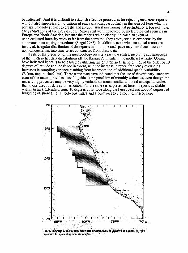
47
be indicated) And it is difficult to establish effective procedures for rejecting erroneous reportswithout also suppressing indications of real variations particularly in the area off Peru which is perhaps uniquely subject to drastic and abrupt natural environmental perturbations For example early indications of the 1982-1983 El Niio event went unnoticed by meteorological agencies in Europe and North America because the reports which clearly indicated an event of unprecedented intensity were so far from the norm that they are rejected as erroneous by the automated data editing procedures (Siegel 1983) In addition even when no actual errors are involved irregular distribution of the reports in both time and space may introduce biases and nonhomogeneities into time series constructed from these data
Tests of the precision of the methodology on interyear time scales involving subsamplings of the much richer data distributions off the Iberian Peninsula in the northeast Atlantic Oceanhave indicated benefits to be gained by utilizing rather large areal samples ie of the order of 10 degrees of latitude and longitude in extent with the increase in report frequency overridingincreases in sampling variance resulting from incorporation of additional spatial variability (Bakun unpublished data) These same tests have indicated that the use of the ordinary standard error of the mean provides a useful guide to the precision of monthly estimates even though the underlying processes may be very highly variable on much smaller temporal and spatial scales than those used for data summarization For the time series presented herein reports available within an area extending some 10 degrees of latitude along the Peru coast and about 4 degrees of longitude offshore (Fig 1) between Talara and a point just to the south of Pisco were
los
Tlara
Chimbote
10oS
M Cullao )U
15S -Ju
200S 1 1 1 1 1 I850W 80-W 75 700 W
Fig 1 Summary area Maritime reports from within the area indicated by diagonal hatching were uIsad foraIssIembli n ontihly samnples
48
composited together These composite samples are assumed to characterize temporal variabilityat least in the relative sense in conditions affecting the neritic fish habitat along that stretch ofcoastline which appears to have some degree of natural unity both in terms of environmentalprocesses and biological community (Santander 1980 Parrish et al 1983) The rather raggedoffshore edge of the summary region was chosen to facilitate initial extraction of the reportsfrom the data archive files Consistent features of spatial variability tend to be much less intensein offshore areas of coastal upwelling regions than in coastal areas thus no substantial effect ofthe irregularity of shape of the offshore boundary is expected Also all the monthly summaries are treated identically in terms of areal selection and so time series homogeneity is preserved Inany case report density is extremely low at the outer edge of the summary area
Assembly of Data Series
Impossible or highly improbable values occur occasionally in the maritime report files dueto keypunch errors etc In the data record format temperature values between -999 and 9990C are possible Initial efforts to construct the data series resulted in rather large standard errors forcertain of the monthly values due to incorporation of improbable data For this reason onlyvalues falling between the limits 11 to 31oC were accepted as valid observations of airtemperature sea surface temperature or wet bulb air temperature for this region (Note that thelower bound on the wet bulb temperature caused only 16 reports no more than a single report inany one month to be rejected) Wind speeds of up to 199 knots (102 msec) are possible in therecord format Erroneously high wind speeds have a particularly serious effect since wind speedis squared in the stress computation and cubed in the wind mixing index formulation Reports ofwind greater than 45 knots (23 msec) occurred within the summary region less than ten times inthe entire 32-year record and were in no case corroborated by neighboring (in either space ortime) data Thus wind reports exceeding this value were excluded in preparing these time seriesThe data record format limited wind direction to values between 0 and 360 degrees cloud coverobservations to the range 0 to 100 of sky obscured and barometric pressure to values between890 and 1070 millibars
In assembling the monthly data samples if any one of the reported values of sea surfacetemperature barometric pressure wind speed or wind direction were missing or unacceptablethe entire report was excluded from the summaries These four observed properties are sufficientto produce time series of sea surface temperature (Table 2) atmospheric pressure (Table 4) windstress components (Tables 5 and 6) and wind mixing index (Table 7) The numbers of reportshaving acceptable observations of these four items are entered as the first of the three numbersshown for each month in Table 1 In addition if a valid cloud cover observation was availablethe report was also incorporated in the cloud cover series (Table 3) numbers of reports includingacceptable observations of these five items are entered as the second number of each monthly setin Table 1Finally if acceptable values of both air (dry bulb) temperature and either wet bulb ordew point temperature were included the report was also used for construction of time series oftmosphere-ocean heat exchange components (Tables 8 to 11) Numbers of available reportscontaining acceptable observations of all seven properties required to construct all the time seriespresented in this paper are shown as the third number under each month in Table 1Allcomputations of derived quantities were performed on each individual report prior to anysummarization process A simple mean was taken as an estimate of the central tendency of eachmonthly sample Computed standard errors of these mean values are displayed within theparentheses following each monthly value presented in the various data tables An approximate95 confidence interval estimate can thus be generated by multiplying the indicated standarderror by the factor 196 and adding and subtracting the result from the monthly mean value(point estimate) to yield the upper and lower limits of the intervalA small percentage of the reports contain wind observations in which the direction is notedas variable ie no direction could be assigned This properly occurs only when the windspeed is very low In these cases the wind speed is used as reported in the calculations where itenters as a scalar quantity ie in the calculations of wind mixing index evaporative heat lossand conductive heat loss In the computation of surface wind stress wind enters as a vector
49
quantity and directionality is crucial Accordingly for the surface wind stress calculationsvariable winds are treated as calms Because the wind speed enters the calculation as a squarelow wind values act essential as zeros in their effect on the monthly means and so treating theseweak variable wind observations as calms has no substantial effect Also the net effect of a stress from one direction is cancelled by an equal stress from the opposite direction and so treating variable-directional stress as equivalent to calm conditions makes physical sense
Sea Surface Wind Stress
Sea surface stress was estimated according to
(ry)= pa CD ( lNto 1Uio 1 101o V10) 1)
where Tx and ryare components of stress directed onshore and alongshore respectively acharacte-istic onshore direction of 62 degrees and an alongshore direction of 332 degrees (fromtrue north) was assigned to the entire summary area Pa is the density of air considered constant at 122 kgm3 CD is a dimensionless drag coefficient 1W10 1 is the wind speed at 10 m heightU10 is the onshore-directed component of wind velocity V10 is the alongshore-directed(positive equatorward) component For the data series presented in the tables CD wasconsidered to be a constant equal to 00013 The use of this constant drag coefficient has been a somewhat standard practice in climatological studies of upwelling regions (Bakun et al 1974Nelson 1977 Parrish et al 1983) However it is recognized that the value of the drag coefficient is actually a variable which depends on the nature of atmospheric turbulence near the seasurface Thus a dependence on both atmospheric stability and wind magnitude near the seasurface is indicated the stability effect is particularly important in reducing air-sea transfers inupwelling regions due to the stable atmospheric boundary layer formed over cool upwelledsurface water No clear consensus as to he proper formulation of these dependencies is presentlyavailable However a reasonable variable drag coefficient formulation has been chosen and hasbeen applied to these data for evaluation of possible differences from results based on the constant drag coefficient formulation In this case we follow the method of Nelson (1977) forincorporation of the atmospheric stability effect which is based on a bulk Richardson number parameterization (Deardorff 1968) We incorporate a dependence on wind speed according to therecommendations of Large and Pond (1981) who find a linear increase in the drag coefficient atwind speeds greater than 11 Imsec
Offshore Ekman Transport
In their climatological study of seasonality and geography of anchovy and sardinereproductive habitats within eastern ocean boundary upwelling systems Parrish et al (1983)found a pattern of minimization of both wind-driven offshore surface flow (Ekman transport)and of wind-induced turbulence in the spawning habits of these fishes They therefore suggestthe likelihood of important effects of both processes on reproductive success Offshore Ekman transport at a given latitude is proportional to the alongshore stress being simply the product ofthe alongshore stress and the reciprocal of the local Coriolis parameter Ekman transport (Ekman1905) provides an acceptable description of ocean surface transport directly driven by surface wind stress at periods which are long compared to the half-pendulum day the half-pendulum dayis 29 actual days in length at 100 latitude but increases to infinity at the equator Obviously theEkman transport description cannot be applied directly at the equator Here we assume theEkman transport description to be adequate for the effect of wind stress variations affecting the summary area as a whole on the monthly time scale thus we simply divide the monthlyalongshore wind stress by a characteristic value of the Coriolis parameter (we choose the localvalue at IOOS ie 00000253sec to characterize offshore Ekman transport in response to largeshyscale long period wind variations over the anchoveta reproductive habitat this choice will affect
so
the average magnitude but not the time series properties of the resulting indicator series which will be identical to those of the alongshore stress series)
Wind Mixing Index
The rate at which the wind imparts mechanical energy to the ocean to produce turbulentmixing of the upper water column is roughly proportional to the third power or cube of thewind speed (Elsberry and Garwood 1978) A wind mixing index which is simply the mean ofthe cube of the observed wind speeds in each monthly sample (Table 7) is presented as a guide tolonger period variability in this particular process However it is to be noted that these series may not reflect energetic shbrter-term variability which may b- more crucial to reproductivesuccess of anchovies (Husby and Nelson 1982) The hypothetical basis for interest in this processin relation to anchoveta reproductive success is Laskers (1978) suggestion that first-feedingsuccess of anchovy larvae may be dependent upon availability of fine scale food particleconcentrations which may be dispersed by wind-driven turbulent mixing events These occur atatmospheric storm event scales which are much shorter than one month Furthermore it is notthe exact magnitude of mixing that is crucial according to this hypothesis but rather theexistence of time-space survival windows within which the rate of addition of turbulence bythe wind does not reach a level that homogenizes the food particle distributions (Bakun andParrish 1980) The wind speed level at which this occurs and the minimum required duration ofthe window for substantial survival to result are unclear and undoubtedly are variable functionsof other factors such as water column stability the particular food particle organisms growthrate behavior motility etc In any case the maritime reports occur irregularly in time and spaceand so are no amenable to indicating durations of periods characterized by specific conditionseven if we were able to specify the required nature of the conditions This would requireutilization of a time-and-space continuous meteorological analysis procedure (Bakun 1986)which might be ineffective due to the low maritime report density in the region and particularlyseaward of the region The use cf shore station data despite interference from local topographicinfluences etc might be the best available option for indicating short time scale wind ariabilityover the ocean habitat off Peru (see Mendo et al this vol)
Solar Radiation
Net incominampsolar radiation QS absorbed by the ocean was estimated according to the formula
QS= ( - a) Qo (I - 062C + 00019h) 2)
where ot is the fraction of incoming radiation reflected from the sea surface Q0 is the sum of thedirect and diffuse radiation reaching the ground under a cloudless sky C is the observed totalcloud amount in tenths of sky covered and h is the noon solar altitude For each maritime reportthe total daily direct solar radiation reaching the ground under cloudless conditions was extractedfrom the Smithsonian Meteorological Tables (List 1949) as a function of the date and latitude ofthe report using a 4 x 4 element curvilinear interpolation on the table entries via Bessels centraldifference formida and assuming the atmospheric transmission coefficient of 07 rezommendedby Seckel and Beaudry (1973) The diffuse solar radiation was estimated according to Listsrecommendations as follows The solar radiation reaching the top of the atmosphere was extracted from the appropriate table This value was decreased by 9 to allow for water vaporabsorption and 2 for ozone absorption The result is subtracted from the value previouslydetermined for the direct radiation reaching the ground to yield the energy scattered out of thesolar beam This is reduced by 50 (to reflect the fact that half is diffused upward and thereforeonly half is diffused downward) to yield the total diffuse solar radiation reaching the ground Thetotal daily direct and diffuse radiation values corresponding to each report are then summed to
51
yield QS The remainder of the computation follows the procedures adopted by Nelson andHusby (1983) The linear cloud correction in Equation (2) is as suggested by Reed (1977) andReeds recommendation that no correction be made for cloud amounts less than 025 of total sky was followed Sea surface albedo was extracted from Paynes (1972) tables following Nelsonand Husbys (1983) algorithm which consists of entering the tables with the 07 atmospherictransmission coefficient rcduced by a factor equal to the linear cloud correction applied inEquation (2) and the mean daily solar altitude The possible error in the net radiation estimateintroduced by using the mean daily solar altitude to indicate albedo rather than an integration over the entire day of entries at short time intervals with instantaneous solar altitudes is estimated to be of the order of 1
Radiative Heat Loss
Effective back radiation is the difference between the outgoing long-wave radiation from the sea surface which depends on the 4th power of the absolute temperature of the sea surface andthe incoming long-wave radiation from the sky which depends on the water vapor content of theatmosphere and on the nature of the cloud cover Here we follow exactly the computationalscheme of Nelson and Husby (1983) who used the modified Brunt equation (Brunt 1932) withthe empirical constants of Budyko (1956) and the linear cloud correction formula of Reed (1976)to compute the effective back radiation (radiative heat loss) QB
-QB = 550 x 10 1 (Ts + 27316) 4 (039- 005ea2)(1 - 09C) 3)
The vapor pressure of the air ea was computed according to the formula provided in the Smithsonian Meteorological Tables (List 1949) using the observed barometric pressure and drybulb and wet bulb air temperatures For reports that were without an acceptable wet bulb temperature but included an acceptable dew point temperature the vapor pressure was computed as the saturation vapor pressure at the dew point temperature using an integrated form of the Clausius-Clapeyron equation (Murray 1967)
Evaporative and Conductive Heat Losses
In estimating evaporative heat loss (latent heat transfer) and conductive heat loss (sensibleheat transfer) the procedures of Nelson and Husby (1983) are again followed closely except for a modification of the wind speed dependence in their variable transfer coefficient formulations as indicated below The bulk aerodynamic formula for turbulent fluxes of latent and sensibleheat across the air-sea interface in a neutrally stable atmospheric boundary layer (Kraus 1972) can be expressed as
QE = Pa LC E(qo - q 1o) 1W10 I 4)
Q =PaCPCH (T3 - Ta) W I 5)
where and I1 are as in Equation (1) with Paassigned the same constant value (122 kgm3) asin the stress computation L is the latent heat of vaporization assigned a constant value of 245 x106 J)kg (5853 calgm) cp is the specific heat of air assigned a constant value of 1000 JkgOC(0239 calgoc) The empirical exchange coefficients CE and CH were assigned constantvalues of 00013 in the construction of the time series presented in Tables 10 and 11 n additiontime series based on variable transfer coefficient formulations incorporating dependencies on atmospheric stability and on wind speed were also assembled for comparison These formulations are again those chosen by Nelson and Husby (1983) which incorporate the
52
atmospheric stability effect according to a bulk Richardson number parameterization (Deardorff1968) however Nelson and Husbys wind speed dependencies were in this case modifiedaccording to the recommendations of Large and Pond (1982) who suggest an increase in CE andCH which is proportional to the square root of the wind speed The specific humidities of the airin contact with the sea surface qO and at 10 m or deck level qi0 were computed according to e
q E-e6)P
where E is the known ratio (a constant equal to 0622) of the molecular weight of water vapor tothe net molecular weight of dry air e is the vapor pressure and P is the barometic pressure Forthis calculation the variation in P is negligible and so a constant value of 101325 pascals(101325 mb) was assigned The calculation of eat 10 m or deck level is as indicated for theradiative heat loss calculation (Equation 3) To calculate e at the sea surface the saturation vaporpressure over pure water was computed from a formula given by Murray (1967) and reduced by2 to account for the effect of salinity (Miyake 1952)
SJ24 A- 350oD
2 300a
lU20 150 U cntn0mM
t 182Ssm 0 50 U)16 -- IJ 9LJL
J F M A M J J A S 0 N D J F M A M J J A S 0 N D
i [M alongshore component
BE 1 onshore component 1_ 1 07shy
1013shy 20esoal-vr0n-LFS 04
-11012-03
0 COL 101 J F M A M J J A S 0 N D 00 ddAS
C F []seasonal ly- varying MLD
12o80 constant 20m MVLD
- o6 shy
04
02 0 5
Ftg 2 Seasonal cycles 32-yr mean monthly values
53
The Seasonal Cycles
The idea of regular seasonal cycles for the coupled ocean-atmosphere system off Peru is to some degree illusory in view of the predominint influence of interyear variability in the regionHowever the seasonal variation is the most cyclic and predictable of the large components of variability It is therefore the conponent of variation which is most likely to be reflected in biological adaptations Accordiz gly a summary of the long-term mean monthly values of the various series (Figs 2 and 3) sen es as a useful starting point for discussion
Being situated within the tropical band the region experiences two passages of the sun each year the sun is directly overhead in October and again in February-March Also since the earths meteorological equator is displaced to the north of the geographical equator the region is dominated by southern hemisphere atmospheric dynamics thus austral winter dominates the seasonality of transfers of momentum and mechanical energy from atmosphere to ocean
The 32-year mean monthly sea surface temperature (Fig 2A) is at a maximum in March coinciding with the second period of vertical sun which marks the culmination of the extended austral summer period of relatively high sun The temperature falls to a minimum in August The atmospheric pressure (Fig 2B) tends to be directly out of phase being at a minimum in the austral summer and at a maximum in the winter season Cloudiness (Fig 2C) lags the atmospheric pressure variation by about one month On average less than 50 of the sky is obscured by clouds in April this increases to greater than 85 in September
The strength of the wind exhibits a typical southern hemisphere seasonality being strongestin austral winter and weakest in summer Thus the 32-year mean monthly values of the index of rate of addition of turbulent mixing energy to the water column (Fig 2D) reach a maximum in August-September and a minimum in January The fact that the seasonal spawning peak of anchoveta is centered within this August-September turbulent mixing maximum would indicate non-adaptation of reproductive strategy for minimization of turbulent mixing effects This is not in accordance with the general pattern suggested by Parrish et al (1983) as generallycharacterizing seasonality and geography of spawning of eastern ocean boundary anchovypopulations Although no claim is made for conclusiveness the inference would seem to be that Laskers (1978) hypothesis is not at least in most years the major factor affecting anchoveta reproductive success off Peru Note that the level of turbulent mixing index intensity off Peru is low compared to other anchovy reproductive habitats even at its seasonal maximum
The alongshore component of wind stress on the sea surface is consistently equatorward in no case in the 32-year series (Table 5) did any monthly wind mean stress value deviate from this predominently alongshore and equatorward tendency in the transfer of momentum from atmosphere to ocean The long-term mean values of alongshore stress (Fig 2E) follow the same seasonal pattern as the turbulent mixing index reaching a maximum in September and a minimum in January The 32-year mean monthly values of the onshore component of stress are small compared to those of the alongshore component but are positive (onshore-directed) at all seasons
Surface Ekman transport being proportional to the alongshore stress but directed perpendicularly to the left of the stress is thus directed offshore with a seasonal maximum againcorresponding to the seasonal spawning peak of anchoveta This anomaly to the pattern of apparent minimization of offshore transport in spawning strategies of engraulids puzzled Bakun and Parrish (1982) However Parrish et al (1983) showed that the seasonal variation in mixed layer depth off Peru proceeds in phase with that of transport in response to the seasonalities in turbulent mixing (Fig 2C) and surface cooling (Fig 2A) but has greater relative amplitude The result is that drifting organisms which are distributed through the upper mixed layer would experience a faster net offshore drift in the thinner surface mixed layer of austral summer than in the deeper mixed layer of winter even though the winter transport (by volume) is much largerThis is illustrated in Fig 2F which shows calculations of mean monthly offshore Ekman velocity of the mixed layer performed in two different ways (based on the 32-year mean monthlyvalues of the data presented in Table 5) Firstly the monthly estimates of offshore Ekman transport are divided by the composite mean (20 m) of the mixed layer depth values given for 2shymonth segments of the seasonal cycle by Parrish et al (1983) Secondly the same monthlyestimates of offshore Ekman transport are divided by monthly mixed layer depth estimates
54
produced by curvilinear interpolation of the 2-month seasonal segments The effect of variable mixed layer depth on the net offshore velocity is apparent and suggestive of adaptation of spawning seasonality for avoidance of offshore loss of larvae (for additional discussion of this aspect see Bakun 1985) The effect of the choice of a constant or variable drag coefficient formulation in the stress computation (Equation 1)on the seasonal signal is indicated in Fig 3AThe 32-year mean monthly Ekman transport values based on the variable coefficient formulation follow a seasonal progression which is very similar to those based on the constant coefficient formulation (ie presented in Table 5) however they are slightly smaller in magnitudereflecting the effect of stability in the atmospheric boundary layer which is stabilized as theonshore-directed airflow is cooled from below while traversing the coastal upwelling zone
Solar radiation entering the ocean (Qs) is at a maximum during the February overhead passage of the sun (Fig 3B) This is due to substantially reduced cloud cover relative to the November solar passage Solar radiation is at a minimum in July when solar altitude has justpassed its June minimum and cloudiness is approaching its winter maximum
30 A constant coeft 6 D 30 m variable coeff E25constant coeff 25 0variable coeff
20
15 E
-10gt
05 10
00 WJ F M A M J J A S 0ON D J F M A M J J A S 0 N D
B250 M constant coef f M variable coeff
0150 04
25100
2 50 5
0 0
C F M A M J J A S O N D J F M A M J J A S O N D
CY~ constant coeff 30-200variable coefV
0154lu
C
Fig 3 Seasonal cycles 32-yr mean monthly values (Note that the SI-standard heat flux units watts per square meter may be converted to calories per square centimeter per day by multiplying by the factor 2604)
55
Heat loss from the sea surface via long-wave radiation (QB) is only a small fraction of theshort-wave radiation absorbed reflecting the areas location within the tropical band (Fig 3C)Radiative heat loss is at a seasonal maximum during April corresponding to the minimum incloudiness and at a minimum in September corresponding to the cloudiness maximum
Heat loss from the ocean via evaporation at the sea surface (QE) is at a maximum duringaustral winter and at a minimum during summer (Fig 3D) The choice of constant or variabletransfer coefficient has only a slight effect with the results of the variable coefficientformulation appearing to increase very slightly in magnitude relative to those of the constant coefficient formulation toward the summer and fall seasons
Heat loss via conduction (Qc) is very small compared to the other heat exchangecomponents (Fig 3) This is fortunate because the choice of transfer coefficient formulationcompletely changes the seasonal pattern With the constant coefficient formulation conductiveheat loss is mostly negative indicating heating of the ocean surface by contact with theatmosphere This reflects the common situation of cool upwelling-affected surface waters beingin contact with a generally warmer atmosphere However the strong stability of the atmosphereboundary layer inherent in this situation inhibits conductive heat transfer according to thevariable transfer coefficient formulation Thus the less common situation where the air is coolerthan the water dominates the sensible heat transfer according to the variable coefficentformulation with the result that conductive heat loss is indicated as being positive in all the 32shyyear composite monthly means except the summer months of January and February
The 32-year monthly means of the time series of atmosphere-ocean heat exchange (QN)which represent the resultant differences between the amount of solar radiation absorbed by the ocean and the sum of the heat losses due to long-wave radiation evaporation and conductionindicate substantial heat gain by the ocean throughout the year (Fig 3F) As expected the average heatgain is greatest in austral summer reaching values of the order of 200 wattsm2(413 cal cm-2 day-1) in January and least in winter falling to about 70 wattsm 2 (144 cal cm-2 day-i) in July The constant coefficient formulations yield slightly greater numerical values ofnet heat exchange than do the variable coefficient formulations mainly due to the differences inthe respective indications of the conductive heat loss component discussed in the previousparagraph however the respective seasonal progressions are very similar
Interyear Variations
If cyclical seasonal effects are those most likely to be adapted for and incorporated in lifecycle strategies of organisms major nonseasonal variations are those most likely to causedisruptions in life cycle processes and therefore to be reflected in population variations Veryshort-scale nonseasonal variations are not well resolved in these monthly composites ofirregularly distributed maritime reports However when shorter period variability is smoothedand the cyclic seasonal effects are suppressed nonseasonal variations of longer than annualperiod which -represent substantial perturbations of the environmental normalcy to whichreproductive strategies or other life cycle strategies should have become tuned are clearlymanifested For the purposes of this discussion a simple 12-month running mean filter is chosen to suppress sea sonalities and smooth the higher frequencies
Problems (negative side lobes wavelength-dependent phase shifts etc) with such equallyshyweighted moving average filters are well known (Anon 1966) However in this case thealternatives also present problems We particularly wish to suppress the seasonal cycle and soweighting the filter elements to suppress side lobes at other frequencies while increasing leakageof the seasonal frequency is not desirable Smoothed monthly series of anomalies from longshyterm monthly means (eg Quinn et al 1978 McLain et al 1985) have the property that thefiltering is nonlocal ie that any value is dependent on other values in the same calendarmonth in temporally distant parts of the time series Thus for example an intense warming(eg El Niiio) occurring within a generally cool climatic period appears as a much less intenseanomaly than a warming of similar magnitude within a warm period also the degree ofindicated intensity changes whenever the length of the series used for determination of the longshyterm mean changes More importantly if the amplitude (or shape phase etc) of the seasonal
56
variation is undergoing nonseasonal variation taking anomalies introduces spurious seasonalshyscale variations into the filtered series A local seasonal filter that avoids some of these problems can be based on 12th-differences eg the result of subtracting from each monthlyvalue the value for the same calendar month in the previous year but the result is therebytransformed to annual rates of change of a property rather than the property itself which complicates a descriptive discussion However the use of 12th-difference transforms is worth considering for empirical modelling efforts For the purposes of this discussion the simple 12shymonth running mean provides a local seasonal filtersmoother which will be familiar to manyreaders and adequate for a descriptive treatment
The filtered sea surface temperature series (Fig 4A) illustrates well the major El Niio warm events of the period 1957-1958 1965 1969 1972-1973 1976 and 1982-1983 Generallyelevated temperatures in the period between the 1976 and 1983 events are also apparent Also apparent is the extended cold period of the mid- 1950s the indication of rise in temperature from this cold period to the peak of the 1957-1983 El Niiio is comparable in total magnitude to that of the rise of the 1982-83 El Ni-io from the much warmer climatic base temperature level of the late 1970s
Major features in the filtered cloud cover series (Fig 4B) are visibly related to those in the temperature series but not in any simple consistent manner Cloud cover minima often appearto coincide with the relaxation of El Nifio events An extraordinarily low degree of cloudings appears to have coincided with the return to normal sea temperatures in 1984 Another sharpcloud cover minimum coincided with the leveling off of the temperature decline following the 1957-1958 event Likewise cloud cover maxima often appear to coincide with rapid drops of temperature into cool periods Atmospheric pressure variations (Fig 4C) are obviously highlyinversely correlated at these low frequencies with those of sea surface temperature
It is not surprising in view of the dynamic linkage of wind to horizontal gradient of atmospheric pressure that wind variations would be related to those of atmospheric pressureThe relation of the wind-cubed index of rate of addition of turbulent mixing energy to the ocean by the wind (Fig 4D) to El Nifio periods is striking El Niffo events are evidently strongwind-mixing events which according to Laskers (1978) scenario would correspond to periodsof high probability of starvation for first-feeding anchoveta larvae The period during and immediately following the 1972 El Nifio appears to have been characterized by an extended period of highly turbulent upper water column conditions The period during and following the 1982-1983 event appears to have been similarly turbulent except for a 2-month window of relaxed turbulent mixing index during December 1983 and January 1984 (somewhat masked bythe smoothing in Fig 4C but evident in the unsmoothed monthly values in Table 7)
The magnitude of alongshore (equatorward) wind stress also increases during El Nifio events (Fig 4E) in agreement with Wyrtkis (1975) conclusions which were based on a summary area displaced somewhat southward along the coast (10-200S 70-80oW) from the oneused here (Fig 1) Thus in addition to potential increases in larval starvation due to increased destruction of food particle strata by turbulent mixing an increase in potential offshore loss of larvae from the favorable coastal habitat is also indicated The onshore component of surface wind stress is relatively small and consistently positive (onshore-directed) in the filtered series
In the previous section the effect of seasonally-varying mixed layer depth on the offshore Ekman velocity of particles which are continually mixed through the upper mixed layer was discussed (ie in reference to Fig 2F) To investigate the effect on interyear time scales filtered time series of offshore Ekman velocity were calculated as in that section ie (i) assuming a constant MLD of 20 m and (ii) assuming a seasonally varying MLD derived from the values given by Parrish et al (1983) The result indicates that at least for the MLD values chosen the effect of seasonally-varying mixed layer depth is such as to substantially increase on average the rate of offshore movement of passive particles in the mixed layer If the effective mixed layerdepth is increased during El Nifio as would be expected both from the effect of the propagatingbaroclinic wave in deepening the surface layer and also from the enhanced wind induced turbulent mixing the effect would be to counteract the increased rate of offshore movement indicated from the Ekman transport calculations
The effect of the choice of constant or variable drag coefficient formulation in the stress computation (Equation 1)is illustrated in Fig 4G where the alongshore stress variation is
25 S24- 28
V)
21
is-1_
55
20
is-__var
60 65
Year
70 75 80
85
020-
---
-1612
-- shy
55
60 65
Year
70
tp
constant coefficientviable coefficient
75 80
-
85
B H
1220 -
- -681 oW210
60
55
56
60 65 Yea
70 75
80
)
85
2 20
u ~190 55 60 65
Year 70
75
80 s
-
85
10135-
13
E10120shy
30
10125-a
010o 55 60 65
Year 70 75 80 85
22
Year
Fig 4 Low-frquency nonseasonal variations 12-month running means of monthly time series values (Note that the SI-standard heat flux units watts per square meter may be converted to calories per square centimeter per day by multiplying by the factor 2064)
-t-4
Ln
D
iso- 80constant 70
coefficientshyvariable coefficient
200
040
B-30 -20shy
55 60 65 Y aYear 80 85 55 60 65 Ya 70 75 80 85
E K
5
Eon~shor
C- 2
tol_
lonshore com ponent copnn --
ID
ISO
160
is 140
12D
I
I00
constant coefficient -
variable coefficient
-
55 60 65 70 75
YeauirY e a r
80 85
~ ~iii~
55 60 65 70
Year -Y 008
75 85
mnl mean lnaitude
2ee e pe ue c pe d by mliyn h factor52064)81b
- seasonally-varying MID ----- e 795 55
6 -
60 0
65 775 80 85 55 60 1 IIl5 I
65 7075 08 Y e ar YYore a -
Fig 4 Continued Low-frequency nonseasonal varitions 12-month running -neans of monthly time series values (Note that the Sl-standard heat flux units watts per square meter may be converted to calories per square centimeter perday by multiplying by the factor 2064)
59
plotted in terms of its directly proportional transform offshore Ekman transport The variable coefficient formulation produces generally lower estimates of stress due to the influence of the stability of the lower atmospheric boundary layer over upwelling-affected surface waters However the differences essentially disappear during the period of relaxation of the intense El Niios of 1957-1958 and 1982-1983 A possible explanation is the tendency for a less stable atmosphere in contact with the ocean surface due to residual warmth which would linger longerin the ocean than in the atmosphere due to the much greater heat storage capacity of water compared to that of air
The filtered series of estimates of absorption of solar radiation by the ocean (QS) exhibits some interesting patterns (Fig 4H) Since the variables that control the solar radiation estimate (Equation 2) derived from a maritime report at any given latitude are calendar date and cloud cover it is not surprising that maxima in Fig 4H often correspond to minima in Fig 4B and vice versa However there are discernible differences between the two series that result from the interaction of the cloud cover variations with the seasonal changes in solar height in the solar radiation time series An impressive feature in the solar radiation series is the early largeshyamplitude alternation consisting of deep minimum of solar radiation entering the ocean corresponding to the early part of the intense 1954-1955 cold period followed by a sharp highlyerratic rise to a high peak in early 1960 In addition the entire period of the 1960s and the first half of the 1970s appears to have been characterized by low absorption of solar radiation relative to the more recent period since 1976
The long-wave radiative heat loss (QB) tends to be an order of magnitude smaller than the short-wave absorption but varies very similarly (Fig 41) This similarity is perhaps explainablein the similar dependence of both types of estimate on cloud cover with the sea surface temperature dependence in the long-wave radiation estimate (Equation 3) being related seasonally to the solar height dependence in the solar radiation estimate (Equation 2) There mayalso be some actual causal effect of the long period variations in solar radiation on the sea temperature dependence in the long-wave radiation estimate
The filtered series of evaporative heat loss (QE) delineates the various El Niffo episodes and the 1954-1955 cold period in a very similar fashion to the sea surface temperature series (Fig4J) The long-term variation in vapor pressure difference between the sea surface and the overlying atmosphere (Equation 4) is apparently very closely linked to that of sea surface temperature As discussed above the wind speed dependence is also a strong function of these climate scale events The effect of choice of constant or variable transfer coefficient apparentlymakes very little difference except during the mid-1950s cold period where increased stability of the air over the cold ocean apparently inhibited the turbulent exchange of latent heat according to the variable coefficient formulation
The net ocean-atmosphere heat exchange series (QN) indicates long-term variations in net ocean heat gain such that minima are associated with El Nifio episodes and maxima with cold periods The variations appear to be controlled to a substantial extent by the evaporative heat loss (Fig 4J) This is so because the variations in heat gain by absorption of short-wave solar radiation (Fig4H) are partially offset by the highly correlated variations in long-wave radiative heat loss (Fig 41) The net effect of the choice of variable or constant transfer coefficient formulations in the evaporative and conductive components is a slight general lowering of the magnitude oi net heat gain in the variable coefficient case This difference is due primarily to the stability effect on the conductive heat loss term as discussed in the previous section in reference to Fig 2E where the average change in the mean net value of this component approximately 5 wattsm2 corresponds in general to the approximate difference between the curves in Fig 4K except in the mid-1950s where stability effects on the evaporative heat loss term are appreciable
In order to check for long-period variations in the distribution of observations within the summary area (Fig 1) filtered series of the monthly averages of the respective latitudinal and longitudinal locations of reports were prepared (Fig 4L) Since the coastline is oriented somewhat northwest to southeast variations in the two curves which tend tc parallel each other in the figure will tend to yield a resultant displacement in the alongshore direction More serious with respect to the long-term homogeneity of the monthly series herein presented are variations in Fig 4L where the curves are changing in the opposite sense ie where the net displacement of the mean position of reports is in the onshore-offshore direction these situations are
60
Table 1 Numbers of observations in monthly samples used to construct timeseries For each month the first number refers to observations used in constructing the values in Tables 2456 amp 7 (sea temperature atmosphericpressure wind stress components and wind cubed index the 2nd number refers to observations used in constructing the values in Table 4 (cloudcover) the 3rd number refers to observations used for values in Tables 8910 amp 11 (heat exchange components)
Jan Feb Mar Apr May Jun1953 21 19 191 29 29 291 22 22 191 23 23 101 33 33 331 16 16 61954 61 57 40 19 19 171 21 21 211 59 59 531 42 39 391 36 34 24 1955 24 22 201 35 35 291 16 15 121 9 9 51 24 24 13 35 35 301956 - 41 38 151 17 15 151 16 16 31 39 39 211 22 22 161 20 20 71957 32 32 321 25 24 151 98 98 471 38 38 291 25 25 211 53 52 33 1958 153 153 1061 74 73 441 69 69 341 84 84 281 67 66 441110 107 521959 128 125 511162 162 491143 138 371115 112 371 97 96 211 67 67 43 1960 98 95 421148 146 1101166 166 1051151 146 1011171 164 1351 85 82 591961 148 147 1271124 124 901115 111 941183 180 1501 89 86 661130 128 1041962 185 183 1271149 148 1341163 162 1421157 155 1221114 111 1051177 177 147 1963 78 76 711103 102 1021182 181 1671180 177 1701157 156 1491185 185 1851964 129 12S 981138 137 1351 82 81 811 76 76 761 45 45 451 52 52 521965 59 59 581 75 71 701137 137 1371 99 99 961139 136 1361139 139 1381966 107 107 1071 82 82 821113 112 1111106 106 1061117 113 1101137 137 137 1967 111 109 1021 60 52 521 80 80 781147 144 1441 75 74 741 66 66 661968 76 76 761128 127 1271108 108 1081139 137 1371 91 87 871111 109 1081969 67 67 67 87 84 841134 131 1311 91 91 911 56 56 561102 102 102 1970 90 87 821 57 57 531103 100 901 51 51 481 99 98 921208 206 200 1971 103 101 931 81 77 751 89 89 891 53 53 521 44 44 441 22 22 211972 109 108 1041 54 52 511 49 49 471 85 85 851 81 81 811 56 56 561973 55 54 401 44 44 391 89 89 891 50 50 481 58 58 561 57 54 471974 84 78 781 63 63 581113 109 1001 57 54 541119 118 1171 73 72 721975 59 57 561 73 72 691140 140 1401 99 92 901140 138 1361116 115 114 1976 70 69 681 20 19 191 76 73 711 59 59 551 71 71 701 49 44 401977 51 51 511109 106 1051 79 79 731101 99 941 93 88 871 70 70 69 1978 57 56 561 65 65 621 71 69 671 92 92 881 71 71 711 41 40 35 1979 97 96 89 58 57 511105 104 981 85 85 771 83 80 741 48 45 341980 96 93 801106 105 931125 123 1021 75 70 541151 146 1191246 201 98 1981 116 113 851 90 89 821139 137 1241108 103 951115 108 791128 124 1081982 91 89 821 90 90 801152 146 1391100 98 881103 98 801 54 54 41 1983 68 64 541126 126 1161 94 91 861 76 72 611 93 92 831 61 61 551984 90 75 261 99 80 391 90 59 141 75 41 161 58 39 61 56 49 29
Jul Aug Sep Oct Nov Dec 1953 10 10 91 39 35 261 29 28 251 18 18 11 24 24 181 19 18 111954 40 39 381 14 14 101 27 26 221 43 371 30 30 61 18 18 9 1955 17 17 121 37 36 211 35 35 61 45 44 341 27 27 201 13 13 51956 45 45 361 21 21 211 29 29 211 41 40 291 63 61 201 24 24 61957 27 27 111 24 24 211 64 64 381112 110 651100 99 531115 115 86 1958 51 51 271159 159 831 96 93 441113 108 471115 110 631 58 43 26 1959 100 100 571103 101 391 85 81 421 74 74 211110 110 551114 114 85 1960 169 168 1471114 111 671142 142 941 75 75 461 63 63 231 82 81 591961 108 107 821155 155 1421153 151 1411128 127 801197 197 1921135 133 118 1962 213 212 1931168 168 1591 81 81 751129 125 1251173 172 1521 91 88 791963 120 120 1201 70 70 701110 110 l011 70 70 701 61 61 581 56 56 53 1964 90 88 871 71 65 641 94 94 881129 127 1211 62 61 581105 104 1021965 92 92 921119 117 1151 99 99 981 67 67 671177 176 1761111 Ill 1061966 116 112 1121122 118 1181185 182 1821131 125 1251 89 89 881123 123 123 1967 89 87 871 67 67 671 84 84 841 76 71 711 73 73 731 99 97 971968 58 58 581 82 81 811 59 59 561111 109 1081118 118 1181 66 65 65 1969 70 70 701 86 84 841108 97 921102 102 971137 137 1271101 101 96 1970 75 74 741 66 65 651 91 90 901 50 50 501127 125 1241 68 68 671971 43 43 421 58 58 541 28 28 231 51 51 471 78 78 781 34 31 30 1972 35 32 301 60 58 541 32 32 291 81 74 741 31 28 261 51 51 48 1973 81 75 741105 92 881 89 84 821 55 54 501100 98 981 71 71 701974 102 101 1011 90 89 891 67 66 661 53 52 501 78 78 771 44 44 441975 67 66 651 53 48 471 70 68 681 70 65 601 68 68 671 88 88 88 1976 74 74 721 21 21 181 88 87 861 76 76 731 46 44 441 58 57 57 1977 55 54 531 55 51 511 73 70 681106 104 1041183 166 1631 67 59 31978 37 33 301 5T S1 501 73 72 671 53 49 491 99 79 761 87 87 851979 80 75 631137 108 q01116 109 821 84 77 531 77 75 591 39 35 26 1980 281 233 53j2tj7 182 9CI148 131 941129 118 891 80 74 611 70 66 471981 169 161 781174 159 631122 111 921127 115 971174 155 1421154 147 127 1982 78 74 681 78 70 661 71 62 551106 102 811132 124 1131 93 89 511983 124 121 841145 116 4F1 70 48 191156 150 901 73 73 241 96 90 321984 104 90 411113 87 81 75 --54 14195 51 69 251 62 40 77 61 35
61
Table 2 Sea surface temperature in degrees Celsius The standard error of the mean appears within parentheses to the right of the mean temperaturevalue
Jan Feb Mar Ap May Jun 1953 2114(50) 2308(64) 2463(51) 2478(49) 2279(37) 2052(46) 1954 1855(33) 2286(46) 2201(42) 1636(29) 1786(23) 1695(25) 1955 2172(39) 1850(52) 2101(85) 1901(37) 1789(85) 1667(30) 1956 1990(44) 1764(82) 2166(46) 2071(29) 1990(41) 1922(29) 1957 1947(47) 2483(48) 2526(21) 2453(37) 2476(48) 2315(27) 1958 2315(11) 2500(19) 2452(25) 2283(30) 2163(35) 2042(18) 1959 2045(21) 2308(18) 2449(15) 2154(25) 2090(18) 1926(25) 1960 2197(18) 2274(18) 2270(19) 2058(18) 1909(14) 1822(18) 1961 2230(15) 2324(20) 2161(21) 1994(15) 2024(21) 1867(15) 1962 2129(14) 2212(18) 2037(18) 1941(18) 1868(18) 1892(12) 1963 2072(24) 2267(17) 2215(16) 2021(17) 2101(13) 1898(10) 1964 2144(12) 2241(14) 2091(22) 2066(37) 1838(26) 1735(24) 1965 2175(26) 2309(27) 2396(15) 2454(21) 2408(20) 2211(14) 1966 2209(20) 2362(20) 2196(25) 2085(24) 1988(24) 1867(16) 1967 2002(22) 2212(22) 2186(23) 2061(19) 1911(24) 1813(30)
1968 1967(21) 2221(21) 2178(22) 1860(20) 1849(30) 1731(20) 1969 2228(23) 2236(23) 2425(18) 2351(23) 2294(25) 2092(22) 1970 2171(26) 2194(43) 2251(26) 2040(33) 1873(21) 1685(14) 1971 1970(19) 2034(29) 1970(25) 2163(36) 1980(32) 1846(46) 1972 2094(25) 2438(41) 2517(37) 2297(24) 23U5(22) 2168(24) 1973 2422(25) 2440(39) 2252(20) 1954(31) 1916(37) 1736(35) 1974 2072(30) 2200(36) 2210(31) 2135(36) 2136(24) 1951(19) 1975 2125(28) 2241(24) 2341(19) 2221(27) 2081(21) 1867(18) 1976 2116(30) 2338(64) 2296(33) 2245(35) 2164(28) 2123(30) 1977 2369(22) 2346(19) 2244(32) 2044(28) 1977(24) 1966(27) 1978 2106(24) 2346(25) 2257(25) 2269(32) 2007(34) 1995(49) 1979 2242(19) 2311(28) 2362(22) 2271(26) 2037(31) 2061(45) 1980 2169(25) 2322(21) 2421(21) 2248(29) 2181(17) 2084(13) 1981 2090(26) 2280(22) 2210(24) 2099(28) 2073(20) 1944(16) 1982 2133(22) 2262(30) 2165(23) 2120(24) 2101(22) 2115(41) 1983 2642(19) 2738(19) 2799(14) 2793(20) 2772(15) 2593(30) 1984 2213(221 2278(291 2192(261 2095(33) 1917(31) 1949f281
Jul Aug Sep Oct Nov Dec 1953 1978(27) 1906(21) 1820(34) 1824(35) 1872(40) 1881(41) 1954 1460(35) 1557(41) 1491(31) 1422(29) 1711(26) 1924(54) 1955 1768(53) 1554(45) 1571(28) 1469(37) 1709(24) 1812(37) 1956 1694(24) 1765(37) 1748(29) 1675(19) 1838(29) 1923(40) 1957 2243(34) 1928(34) 1894(19) 1923(17) 1907(16) 2075(16) 1958 1963(26) 1737(10) 1780(15) 1790(13) 1898(18) 2025(31) 1959 1755(15) 1680(12) 1664(18) 1777(20) 1904(20) 1935(15) 1960 1765(10) 1742(12) 1717(11) 1753(18) 1878(24) 2059(17) 1961 1004(22) 1762(11) 1687(11) 1736(16) 1854(14) 1939(17) 1962 1730(09) 1727(10) 1677(10) 1689(10) 1808(12) 1949(21) 1963 1870(13) 1824(17) 1800(11) 1755(16) 1854(28) 1972(17) 1964 1710(18) 1611(20) 1611(14) 1640(15) 1831(32) 1976(19) 1965 2059(20) 2000(20) 1779(16) 1826(23) 1876(13) 2149(15) 1966 1800(12) 1675(13) 1681(10) 1737(12) 1813(17) 1977(20) 1967 1740(16) 1646(17) 1S76(13) 1609(21) 1690(18) 1822(21) 1968 1764(23) 1705(17) 1826(38) 1765(17) 1767(16) 2082(24) 1969 1844(20) 1801(17) 1736(19) 1824(16) 1839(13) 1949(15) 1970 1572(12) 1619(13) 1633(28) 1636(25) 1794(16) 1829(21) 1971 2800(28) 1727(23) 1632(26) 1705(27) 1834(15) 1981(35) 1972 2118(36) 2177(23) 1929(36) 1917(35) 2061(32) 2173(31) 1973 1688(32) 1604(16) 1580(22) 1611(31) 1727(24) 1901(30) 1974 1812(15) 1748(15) 1670(31) 1691(32) 1896(23) 1983(35) 1975 1846(25) 1768(36) 1571(24) 1559(20) 1624(15) 1874(24) 1976 2118(20) 1951(55) 1900(23) 1919(25) 2004(23) 2146(15) 1977 1854(25) 1723(22) 1721(28) 1849(28) 1895(16) 1945(24) 1978 1849(35) 1691(33) 1727(25) 1811(25) 1940(30) 2049(24) 1979 1873(25) 1830(26) 1901(28) 1853(23) 1925(27) 2104(38) 1980 2004(11) 1835(13) 1777(15) 1839(23) 1895(27) 2021(21) 1961 1808(17) 1824(11) 1767(24) 1786(23) 1898(15) 2029(15) 1982 1965(18) 1834(23) 1900(36) 2061(22) 2303(17) 2519(21) 1983 2324(23) 2126(21) 1957(25) 1989(14) 2025(22) 2154(27) 1984 1952(231 1837(131 1844(18) 1827(281 1970(311 2020(311
62
Table 3 Total cloud amount Valvas indicate mean fraction of sky obscuredThe standard error of the mean appaars in parentheses to the right of each mean value
Jan Feb Mar ApM May1953 66(06) s8(06) 43(06) 43(08) 54(06)
Jun 76(10)1954 59(05) 75(05) 69(07) 35(04) 85(05) 74(07)1955 55(07) 61(06) 60(09) 06(04) 69(08) 90(04)1956 66(05) 46(l0) 40(06) 33(06) 65(08) 89(06)
1957 48(07) o(05) 56(03) 57(05) 5(06) 76(04)1958 60(03) 68(03) 63(03) 32(04) 54(04) 83(03)1959 40(03) 58(C2) 66(02) 60(03) 83(03) 78(04)1960 so(03) 30(03) 38(02) 44(03) 52(03) 63(05)1961 65(03) 44(03) 65(03) 50(03) 49(04) 79(03)1962 55(02) 54(03) 48(03) 56(03) 53(04) 79(03)1963 50(04) 52(03) 61(02) 52(03) 66(03) 81(02)1964 64(03) 66(03) 57(04) 51(04) 72(06) 63(06)1965 54(04) 49(04) 61(02) 60(03) 63(03) 64(03)1966 56(03) 44(03) 57(03) 45(03) 62(03) 76(03)1967 72(03) 51(05) 56(03) 51(03) 46(04) 82(04)1968 52(04) 52(03) 45(03) 38(03) 65(04) 75(03)1969 57(04) 55(04) 58(03) 57(04) 70(05) 81(03)1970 59(04) 43(04) 37(03) 43(05) 62(04) 81(02)1971 51(03) 3s(04) 48(03) 52(05) 68(06) 8s(06)1972 53(04) 49(04) 64(03) 53(04) 69(04) 78(04)1973 67(03) 61(05) 60(04) 49(04) 40(05) 70(05)1974 59(03) 52(04) 53(03) 53(05) 77(03) 8(02)1975 69(04) 50(04) 60(02) 54(03) 72(03) 86(03)1976 61(04) 59(08) 63(03) 55(05) 62(04) 87(04)1977 54(05) 68(03) 55(04) 34(03) 53(04) 71(04)1978 53(04) 65(04) 45(04) 57(04) 54(05) 68(07)1979 s0(03) 53(04) 56(03) 44(03) 67(04) 79(05)1980 57(03) 53(03) 58(03) 48(04) 57(03) 80(02)1981 66(03) 63(03) 51(03) 57(03) 66(03)1982 80(03)
60(03) 58(03) 55(03) 52(03) 58(04) 84(04)1983 52(04) 47(02) 63(03) 70(03) 75(03) 74(04)1984 42(041 43(031 45(03) 40(04) 34(051 74(041
Jul Aug SeD Oct NOV Dec1953 65(14) 91(04) 74(07) 74(07) 81(06) 67(07)1954 79(05) 86(07) 92(05) 89(04) 72(05) 75(08)1955 97(02) 90(04) 90(04) 80(05) 61(08) 44(10)1956 85(05) 82(08) 64(05) 62(05) 73(05) 49(08)1957 79(06) 72(08) 85(04) 72(03) 72(03) 64(03)1958 79(05) 80(03) 90(02) 81(03) 52(04) 45(06)1959 78(03) 78(03) 79(04) 79(03) 63(04) 51(03)1960 72(03) 81(03) 90(02) 89(03) 63(05) 67(04)1961 94(01) 83(02) 90(02) 78(03) 61(02) 60(03)1962 90(02) 93(02) 86(03) 88(02) 77(02) 46(04)1963 80(03) 80(04) 88(02) 82(04) 77(04) 68(05)1964 87(03) 87(03) 86(03) 88(02) 77(04) 51(03)1965 88(03) 90(02) 92(02) 86(03) 75(02) 61(03)1966 77(03) 83(03) 85(02) 89(02) 83(03) 61(03)1967 88(03) 91(03) 84(03) 85(04) 86(03) 47(04)1968 80(05) 93(02) 88(03) 83(03) 76(03)1969 86(04) 83103) 91(02) 82(03) 68(03) 50(04)
56(04) 1970 87(04) 91(03) 85(03) 95(02) 59(03) 64(04)1971 94(02) 88(03) 92(03) 853(05) 65(04) 65(06)1972 83(05) 80(04) 87(04) 78(04) 86(05) 67(05)1973 82(03) 91(02) 87(03) 80(04) 81(03) 72(04)1974 91(02) 89(03) 88(03) 75(05) 72(04) 57(05)1975 86(03) 89(03) 89(03) 77(04) 78(04) 64(04)1976 80(04) 93(03) 77(03) 81(03) 78(04) 53(04)1977 89(03) 86(04) 83(04) 81(03) 72(02) 41(05)1978 9s(0l) 84(04) 80(104) 8l(04) 68(04) 50(03)1979 865(03) 8l(03) 83(03) 8(03) 8o(03) 49(06)1980 90(01) 90(02) 81(02) 82(02) 69(04) 48(04)1981 87(02) 83(02) 92(02) 67(03) 63(03) 51(03)1982 80(04) 88(03) 82(03) 76(03) 75(03) 58(03)1983 72(03) 68(03) 66(06) 80(02) 58(04) 49(04)1984 81(031 75(031 86(031 91(03 70o051 52(041
63
Table 4 Atmospheric pressure at sea level Add 10000 to the mean valuesin the table to yield pressure in millibars The standard error of the mean appears in parentheses to the right of each mean value the standard errors are given (directly) in millibars
Jan Feb Mar A r May Jun1951J 112( 3) 104( 1) 111( 3) 132( 5) 125( 2) 145( 5)1954 123( 2) 122( 4) 102( 4) 213( 3) 135( 3) 147( 3)1955 125( 3) 109( 2) 104( 4) 119( 5) 136( 2) 152( 2)1956 115( 2) 107( 4) 111( 3) 109( 3) 120( 2) l0O( 6)1957 128( 2) 86( 3) 109( 3) 99( 3) 123( 2) 123( 2)1958 219( 2) 115( 2) 72( 4) 98( 3) 115( 2) 132( 1)1959 120( 2) 109( 1) 115( 2) 112( 1) 133( 2) 142( 2)1960 116( 2) 215( 2) 113( 2) 115( 1) 127( 1) 137( 2)1961 106( 4) 106( 2) 106( 2) 112( 4) 129( 1) 136( 2)1962 130( 1) 118( 2) 120( 1) 128( 2) 140( 2) 153( 1)1963 129( 2) 136( 2) 112( 1) 135( 4) 132( 1) 142( 1)1964 23( 1) 105( 1) 112( 2) 122( 2) 127( 4) 142( 2)1965 117( 1) 102( 2) 110( 2) 115( 1) 113( 2) 129( 2)1966 106( 2) 102( 2) 202( 1) 118( 2) 132( 1) 146( 1)1967 115( 2) 123( 2) 120( 2) 113( 2) 131( 2) 143( 2)1968 113( 2) 117( 1) 126( 2) 129( 1) 143( 2) 156( 1)1969 112( 3) 96( 1) 114( 2) 113( 1) 115( 2) 13s( 2)1970 128( 2) 110( 2) 118( 1) 117( 2) 145( 2) 144( 1)1971 119( 2) 108( 2) 108( 2) 123( 2) 138( 3) 153( o4)1972 109( 2) 210( 3) 103( 2) 115( 2) 118( 2) 121( 2)1973 105( 4) 118( 2) 107( 2) 115( 3) 130( 3) 145( 2)1974 119( 5) 118( 2) 125( 2) 126( 3) 137( 3) 142( 2)1975 115( 3) 119( 2) 114( 1) 119( 2) 135( 1) 140( 1)1976 121( 3) 116( 7) 106( 1) 119( 2) 125( 2) 120( 2)1977 204( 3) 212( 1) 100( 2) 120( 4) 126( 2) 137( 2)1978 139( 3) 101( 7) 120( 2) 123( 2) 128( 2) 150( 3)1979 122( 1) 119( 3) 114( 2) 110( 3) 133( 3) 155( 5)1980 129( 2) 123( 2) 93( 2) 105( 2) 129( 2) 145( 3)1981 139( 3) 108( 2) 114( 2) 121( 2) 143( 2) 18( 4)1982 126( 5) 114( 2) 104( 2) 121( 2) 126( 2) 129( 3)1983 91( 3) 97( 2) 91( 2) 95( 2) 96( 3) 116( 2)1984 125(21 107( 3) 107( 51 131f 3 137( 7) 139( 21 1953 137( 5) 134( 2) 130( 2) 150( 5) 140( 3) 132( 4)1954 138( 3) 143( 4) 138( 3) 148( 2) 145( 2) 130( 3)1955 157( 3) 151( 3) 154( 3) 161( 3) 140( 2) 131( 5)1956 149( 3) 137( 4) 144( 3) 141( 2) 142( 5) 94( 6)1957 130( 3) 140( 3) 125( 3) 134( 2) 128( 2) 122( 2)1958 141( 3) 139( 2) 140( 3) 127( 2) 128( 2) 106(l7)2959 136( 1) 141( 2) 131( 2) 137( 2) 133( 2) 122( 3)1960 145( 1) 145( 2) 141( 1) 140( 2) 111( 2 135( 3)1961 144( 2) 144( 1) 147( 1) 13b( 1) 147( 2) 132( 1)1962 144( 1) 152( 2) 139( 3) 153( 2) 106(14) 138( 2)1963 143( 2) 136( 3) 138( 4) 144( 1) 154( 4) 124( 2)1964 148( 1) 148( 2) 142( 2) 143( 2) 131( 2) 132( 1)1965 126( 2) 140( 2) 141( 2) 139( 2) 121( 2) 116( 1)1966 140( 1) 149( 1) 148( 1) 141( 2) 136( 2) 123( 1)1967 142( 2) 145( 2) 152( 2) 140( 2) 134( 2) 130( 2)1968 148( 2) 152( 1) 140( 3) 135( 2) 141( 1) 126( 2)1969 143( 2) 149( 2) 130( 1) 138( 1) 132( 2) 122( 1)2970 155( 1) 144( 2) 138( 2) 139( 3) 139( 1) 110( 2)2971 137( 3) 143( 7) 145( 4) 153( 2) 140( 1) 123( 3)1972 125( 6) 128( 3) 129( 3) 131( 2) 122( 3) 218( 6)1973 147( 4) 148( 2) 152( 3) 151( 2) 143( 2) 148( 2)1974 138( 4) 147( 2) 149( 2) 140( 2) 137( 1) 126( 2)1975 152( 2) 151( 3) 155( 2) 153( 2) 151( 2) 135( 2)1976 133( 2) 146( 6) 133( 4) 137( 3) 139( 2) 104( 2)1977 135( 3) 143( 2) 147( 2) 142( 2) 137( 2) 124( 2)1978 139( 4) 141( 2) 145( 2) 138( 2) 123( 2) 123( 2)1979 149( 2) 142( 3) 147( 3) 148( 2) 141( 3) 125( 9)1980 151( 2) 152( 2) 141( 4) 138( 3) 138( 2) 137( 5)1981 150( 3) 160( 2) 148( 2) 139( 2) 134( 2) 119( 1)1982 120( 2) 129( 2) 141( 3) 129( 2) 106( 2) 100( 2)1983 118( 2) 142( 4) 150( 5) 136( 2) 133( 7) 142( 4)1984 126( 4 153( 31 148( 51 145( 31 142( 11 118( 31
64
Table 5 Alongshore component (positive equatorward) of wind stress on the sea surface Units are dynes per square centimeter The standard error of the mean appears in parentheses to the right of the mean alongshore stress valueValues in this table multiplied by the factor 395 (see text) yield offshoreBkma transport in cubic meters per second across each meter width
Jan FeP Mar A P May Jun 1953 36(06) 32(05) 44(07) 99(20) 83(09) 37(10)1954 24(03) 41(14) 10(02) 46(05) 56(08) 46(08) 1955 40(09) 16(03) 53(18) 18(08) 63(11) 45(09)1956 16(02) 25(07) 67(10) 83(09) 85(13) 50(05)29S 31(06) 53(21) 76(05) 86(10) 57(06) 76(07) 1958 40(05) 42(05) 45(05) 61(06) 57(07) 46(04)1959 34(03) 28(02) 40(03) 42(04) 30(03) 59(07)1960 23(03) 27(02) 41(03) 49(04) 53(09) 45(04)1962 20(02) 27(03) 39(04) 48(03) 70(06) 48(05)1962 42(02) 34(03) 47(03) 52(04) 51(04) 60(04)1963 32(04) 39(03) 61(03) 47(03) 59(04) 33(03)1964 49(04) 44(03) 51(05) 71(07) 63(07) 58(12)1965 29(04) 40(05) 40(03) 53(06) 97(07) 58(04)1966 60(04) 61(06) 46(04) 75(06) 59(05) 62(04)2967 40(04) 36(04) 29(03) 30(03) 37(04) 71(10)1968 15(02) 40(05) 36(03) 36(03) 34(05) 65(05)1969 29(04) 26(04) 47(04) 56(04) 45(07) 89(08)1970 33(04) 16(05) 40(05) 56(06) 55(05) 52(04)2971 17(04) 36(04) 34(03) 59(08) 43(07) 73(23)1972 29(03) 34(04) 56(11) 55(04) 42(04) 67(08)1973 57(06) 38(05) 73(05) 60(08) 67(11) 51(07)1974 32(04) 42(05) 48(04) 68(07) 71(05) 66(07)1975 40(04) 35(04) 72(05) 63(05) 74(04) 63(06)1976 21(04) 17(04) l(05) 77(07) 72(07) 56(08)1977 32(06) 56(06) 38(04) 57(05) 47(05) 67(05)1978 37(05) 47(06) 62(07) 71(08) 59(07) 72(12)2979 49(05) 54(09) 54(04) 68(05) 69(07) 92(14)1980 44(04) 47(05) 49(04) 49(05) 89(07) 58(03)2981 52(04) 30(03) 46(04) 54(04) 53(05) 84(08)1982 35(04) 47(04) 63(04) 55(04) 65(06) 91(12)1983 69(06) 66(04) 46(05) 74(08) 75(06) 107(09) 1984 26(041 53(111 80(131 31(11) 83(181 07(131
Jul Aug See Oct No Dec 1953 70(22) 36(05) 46(06) 53(08) 62(08) 27(05)1954 52(07) 89(21) 83(09) 24(02) 30(04) 20(04)1955 46(09) 88(14) 66(10) 65(12) 60(08) l1(04)1956 69(09) 52(13) 64(05) 50(C8) 45(04) 45(08) 2957 101(11) 54(08) 75(07) 56(06) 44(04) 56(04)2958 51(05) 71(06) 49(04) 43(04) 26(03) 39(05)1959 38(04) 53(04) 48(07) 44(05) 31(03) 23(03)1960 59(05) 55(04) 51(04) 48(06) 34(03) 36(04)1961 67(06) 50(04) 50(04) 40(03) 38(02) 31(03)1962 60(04) 49(04) 60(06) 49(04) 51(04) 23(02)1963 54(05) 48(06) 72(05) 72(11) 53(06) 36(04)1964 62(05) 71(09) 73(08) 57(04) 36(05) 42(04)1965 63(05) 84(07) 87(07) 60(07) 49(03) 49(04)1966 76(04) 74(06) 59(03) 52(04) 26(03) 26(02)1967 54(05) 72(07) 74(09) 73(09) 46(05) 35(06)1968 90(10) 72(08) 64(08) 59(03) 51(03) 62(08)1969 53(06) 71(08) 59(05) 42(04) 28(03) 37(04)1970 1971
47(06) 52(05) 45(04) 50(07) 41(03) 27(05)40(08) 77(112) 64(12) 71(08) 43(05) 49(09) 1972 90(11) 81(10) 132(19) 49(05) 35(04) 72(15)1973 70(11) 116(12) 101(11) 71(09) 58(05) 37(06)2974 73(05) 64(08) 72(07) 67(07) 68(05) 45(06)1975 64(07) 91(10) 73(05) 51(05) 36(04) 35(05)1976 59(05) 69(16) 80(06) 67(06) 64(06) 52(06)1977 94(11) 83(10) 47(06) 46(04) 157(04) 55(o06) 1978 87(14) 69(08) 73(09) 54(06) 51(06) 47(05)1979 65(07) 66(09) 72(07) 65(05) 54(05) 46(07)1980 101(04) 74(04) 75(06) 65(05) 47(04) 49(06)1981 77(07) 64(04) 85(09) 41(04) 57(04) 42(03)1982 89(08) 63(06) 96(12) 84(06) 73(04) 66(05)2983 86(06) 69(06) 77(07) 60(05) 38(10) 23(05)1984 61(061 76(061 64(071 60(041 86f061 58(05)
Table 6 Onshore component of wind stress on the sea surface Units are dyres per square centimeter The standard error of the mean appears in parentheses to the right of each mean onsho7e stress value
1953 1954 1955
Jan 10(03) 04(0)
-04(03)
Fab 02(03) 07(05)02(01)
Mar 00(05) 00(01)19(07)
APr -12(04) 10(02)09(08)
May 02(04)
-04(03)-01(03)
Jun -06(05) 04(02)
-01(03)
1956 1957 1958 1959 1960 1961 1962
06(03)
05(02)
07(01)
05(01)
07(01)
03(01)
08(01)
48(03) -06(05) 08(02) 07(01) 04(01) 01(01) 01(02)
o8(08) -06(02) 09(02) 01(02) 05(ol) 06(02) 04(01)
01(04) -04(03) 01(02) 06(01) 04(02) 05(01) 02(02)
0(05)
00(04)
02(02)
04(02)
03(01)
03(02)
02(02)
10(04)
06(03)
08(02)
17(03)
02(02)
04(02) -03(01)
1963 1964 1965
06(01)
05(02)
06(02)
02(02)
03(01)
05(02)
08(01)
04(02)
01(01)
01(01) -07(03) 06(02)
0(02)
CL(04) -08(03)
01(01)
06(03)
03(02) 1966 1967 1968
05(02)
02(02)
03(01)
06(02)
08(02)
02(02)
09(03)
02(02)
04(01)
-06(02) 03(01) 02(01)
03(02)
09(02)
01(03)
06(02)
08(05)
01(02) 1969 1970 1971 1972 1973 1974 1975 1976 1977 1978 1979 1980
04(01)
04(02)
05(02)
04(01)
13(03)
04(02)
02(02)
03(01)
07(02)
04(03)
03(02)
08(02)
04(02) -08(05) 04(02)
-06(05) 07(02) 02(02) 07(02) 01(04)
-03(03) 09(03)
-08(04) 06(02)
00(01)
05(02)
00(02) -06(07) -02(02) -04(02) -05(02) 01(02) 06(02) 05(03) 08(03) 02(02)
03(02)
10(03)
03(04)
03(02)
13(04)
02(04) -04(02) -06(04) 07(03)
-03(02) 03(02) 03(03)
05(03)
08(02) -03(02) 00(02)
-02(04) -01(02) 00(02) 01(02) 02(02) 03(02)
-03(03) -05(03)
-03(03) 03(01)
-08(07) 06(04) 15(05) 03(03)
-01(02) 03(04)
-01(03) -07(05) -04(04) -08(02)
1981 1982 1983 1984
02(02)
06(02)
15(03)
06(02) Jul
00(02)
1O(03)
00(02) -04(021
Aug
05(02)
00(02) -03(03) -08(061
Sep
-01(02) -O1(02) -01(07) -10(061
Oct
01(02)
06(03)
07(03)
08(07) NOv
01(03) -09(06) 05(04) 14(051
Dec 1953 1954
15(04)
06(03) 06(02)
-02(ll) 12(03) 19(08)
07(07)
04(01) 08(03) 21(05)
04(02)
08(02) 1955 1956 1957 1958 1959 1960 1961 1962
o8(04)
02(06) -05(09) 12(03) 04(02) 06(02) 04(02) 05(01)
04(06)
31(08)
18(05)
23(05)
12(02)
07(02)
03(01)
12(02)
09(04)
13(04)
05(03)
12(02)
17(06)
06(02)
08(02)
10(02)
09(02)
14(03)
07(02)
20(03)
05(01)
67(02)
15(03)
08(02)
12(05)
06(03)
10(02)
05(01)
05(01)
02(01)
03(01)
08(01)
o5(ol)
06(02)
11(02)
06(02)
04(01)
06(02)
04(01)
09(02) 1963 03(02) 01(02) 09(02) 05(03) 03(04) 07(02) 1964 1965 1966 1967 1968 1969 1970 1971
04(02)
01(03)
05(02)
tB(02)
3(04)
02(02)
07(02)
01(03)
05(05) -02(02) 15(03) 06(04) 09(03)
-02(02) 08(02) 14(04)
10(03)
10(03)
08(02) -01(03) 12(05) 08(02) 10(02)
-01(03)
11(02)
17(04)
15(02)
09(03)
11(02)
04(01)
18(04)
00(03)
05(02)
13(03)
06(01)
03(02)
08(01)
07(01)
12(03)
06(02)
04(02)
08(02)
02(01)
12(03) -06(04) 09(02) 09(03)
-02(04) 1972 1973
04(04) -03(04)
07(03)
01(05) 12(08) 01(06)
10(03)
01(05) 19(04) 01(02)
14(03)
06(03) 1974 1975
02(02)
06(03) 04(03) 03(05)
13(03)
06(03) 12(03) 11(03)
03(03)
os(03) 13(03) 04(02)
1976 1977 1978 1979
03(04)
05(07) -11(05) -01(03)
-01(06) -10(04) 04(04) 10(03)
09(03)
10(03)
07(03) -02(04)
15(03)
08(02)
08(03)
07(02)
02(04)
07(01)
07(02)
oo(03)
13(04)
02(03)
05(02)
06(06) 1980 1981 1982 19831984
-12(02) -04(03) 05(04) -03(02)07(051
-02(03) -05(01) 04(02)
-o(03) -22051
04(03)
01(03)
01(06) -10(03)03(04)
05(02)
07(02)
15(04)
02(03)02(041
06(02)
05(02)
09(02)
04(03)-09(031
-01(02) -04(01) 08(02) 04(03)-01(031
66
Table 7 Wind cubed index of rate of addition to the water column bywind of turbulent mixing energy the
The standard errors of the mean appear inparentheses to the right of each mean index value 3 3 Nominal units are m sec
Jan Feb Mar Aot may Jun1953 130( 34) 107( 19) 162( 35) 473(140) 354( 44) 130( 47)1954 75( 16) 205( 85) 19( 4) 186( 32) 210( 46) 174( 41)1955 132( 40) 37( 9) 316(101) 93( 22) 238( 67) 177( 50)1956 58( 15) 91( 30) 287( 46) 355( 51) 377( 68) 182( 25)1957 201( 22) 220( 44) 310( 23) 375( 64) 201( 27) 337( 42)2958 184( 48) 171( 32) 181( 25) 260( 37) 244( 46) 192( 21)1959 116( 13) 94( 8) 143( 14) 154( 18) 104( 16) 300( 47)1960 84( 11) 86( 10) 151( 15) 207( 18) 307( 95) 161( 19)1961 71( 9) 83( 11) 173( 24) 17C( 13) 301( 37) 204( 26)2962 156( 12) 127( 16) 171( 14) 220( 24) 197( 20) 226( 19)1963 113( 19) 141( 19) 252( 17) 176( a) 230( 20) 113( 13)1964 188( 20) 156( 14) 198( 27) 295( 36) 248( 41) 315(117)1965 100( 17 155( 33) 144( 16) 238( 51) 467( 45) 232( 20)1966 247( 26) 263( 30) 213( 25) 312( 35) 252( 34) 263( 24)1967 147( 16) 143( 25) 94( 13) 102( 11) 140( 20) 387( 80)1968 47( 10) 172( 3G) 126( 15) 120( 11) 142( 25) 272( 25)1969 97( 16) 113( 19) 174( 18) 206( 23) 193( 34) 432( 68)1970 121( 17) 148( 36) 166( 3R) 232( 35) 227( 25) 218( 20)1971 92( 16) 128( 25) 120( 15) 266( 42)1972 102( 14) 146( 33) 346( 70)
135( 30) 404(162)214( 25) 146( 18) 315( 51)2973 247( 29) 136( 21) 292( 26) 333( 49) 314( 75) 279( 52)1974 121( 17) 155( 24) 181( 20) 308( 62) 300( 29) 295( 39)1975 135( 18) 140( 22) 308( 24) 251( 21) 304( 24) 272( 33)1976 76( 22) 68( 19) 196( 27) 326( 39) 308( 36) 248( 53)1977 134( 44) 251( 40) 158( 21) 265( 27) 191( 27) 263( 30)1978 150( 22) 214( 33) 280( 44) 316( 54) 246( 35) 327( 91)1979 202( 33) 250( 54) 241( 23) 282( 29) 331( 38) 459(122)1980 179( 19) 212( 32) 203( 21) 194( 23) 441( 47) 241( 18)1981 205( 22) 104( 13) 195( 19) 212( 21) 226( 27) 431( 73)1982 134( 21) 199( 20) 259( 19) 201( 20) 300( 29) 491( 97)1983 319( 31)1984 110( 211 262( 18) 203( 21) 420(117) 373( 35) 539( 61)307(120) 534M17 288f110) 636(1591 522(1161
Jul Aug San Oct Nov Dec1953 332(129) 125( 26) 179( 34) 217( 43) 243( 50) 74( 16)1954 207( 37) 445(135) 439( 73) 64( 8) 161( 33) 59( 13)1955 179( 41) 460(100) 308( 76) 322( 79) 266( 42) 30( 13)1956 324( 56) 346( 65) 261( 29) 237( 56) 184( 23) 158( 35)1957 484( 66) 253( 52) 331( 45) 261( 38) 189( 24) 238( 22)1958 214( 25) 474( 56) 214( 26) 228( 30) 92( 16) 152( 26)2959 138( 16) 233( 23) 303( 76) 164( 23) 108( 15) 82( 13)1960 260( 32) 222( 25) 201( 19) 198( 35) 99( 12) 144( 24)2961 290( 39) 191( 17) 211( 20) 199( 24) 136( 12) 100( 12)1962 265( 22) 236( 23) 267( 32) 199( 20) 212( 19) 96( 15)1963 220( 26) 176( 25) 320( 31) 376( 72) 222( 33) 131( 19)1964 250( 25) 385( 89) 372( 58) 242( 22) 132( 20) 164( 21)1965 263( 29) 392( 45) 442( 52) 319( 44) 240( 21) 193( 20)1966 317( 29) 388( 39) 245( 18) 243( 28) 95( 12) 83( 10)1967 222( 28) 336( 41) 357( 59) 369( 57) 180( 30) 280( 45)2968 442( 61) 352( 56) 326( 62) 243( 19) 192( 16) 283( 42)1969 237( 33) 312( 52) 272( 29) 154( 26) 104( 13) 151( 23)1970 248( 34) 212( 28) 186( 22) 251( 50) 194( 24) 139( 22)1971 190( 49) 425( 71) 258( 66) 302( 49) 169( 23) 199( 57)1972 423( 63) 400( 67) 805(139) 220( 27) 156( 25) 407(157)1973 S69( 81) 784( 81) 675( 74) 348( 66) 237( 28) 179( 37)197v 299( 28) 317( 57) 352( 45) 295( 42) 274( 28Y 195( 31)1975 284( 35) 461( 58) 316( 31) 235( 35) 143( 24) 147( 23)1976 264( 36) 377( 87) 370( 33) 328( 37) 270( 49) 235( 43)2977 529( 95) 392( 59) 229( 37) 189( 21) 241( 17) 220( 34)1978 434( 85) 310( 54) 350( 82) 226- 29) 237( 49) 203( 28)1979 290( 51) 433( 73) 350( 51) 274( 33) 233( 28) 226( 50)1980 458( 27) 354( 31) 382( 35) 271( 28) 181( 22) 188( 30)1981 420( 49) 244( 21) 457( 60) 166( 10) 249( 22) 146( 13)1982 438( 52) 270( 40) 549( 82) 454( 57) 316( 22) 275( 30)1983 379( 34) 330( 39) 318( 43) 277( 33) 227(111) 122( 32)1984 334i 58) 415( 881 328( 461 242( 30) 350( 27) 229( 221
67
Table 8 Daily total (both direct and diffuse) solar radiation absorbed bythe ocean Qs The standard error of the mean appears in parentheses to theright of each sean yalue Units are wattsM 2 (Values may be converted tounits of cal c ay by multiplying by the factor 2064)
Jan Feb Mar Aor May239(12) 253( 9) 262(11) 258(15)
Jun1953 193( 9) 182(22)1954 240( 9) 214(10) 227(12) 241( 6) 141( 7) 158(11)1955 250(12) 254(12) 236(17) 282( 8) 182(17) 125( 5)1956 255(16) 269(16) 257(31) 230(12) 181(14) 121( 3)1957 264(12) 203(11) 243( 7) 221( 8) 190(10) 153( 7)1958 244( 5) 236( 8) 243( 9) 248( 9) 202( 8) 148( 6)1959 287( 7) 247( 8) 241( 9) 208(10) 169(12) 144( 6)1960 268( 9) 269( 4) 283( 3) 236( 4) 204( 4) 167( 7)1961 242( 5) 276( 5) 228( 5) 221( 4) 205( 6) 140( 4)1962 258( 5) 257( 4) 260( 4) 214( 4) 192( 6) 143( 3)1963 263( 6) 265( 5) 240( 4) 217( 0) 176( 4) 139( 3)1964 243( 6) 236( 4) 242( 6) 223( 6) 162( 8) 161( 7)1965 257( 8) 268( 7) 236( 4) 218( 4) 183( 4) 165( 4)1966 252( 5) 279( 5) 246( 5) 236( 4) 182( 5) 148( 4)1967 218( 5) 264( 8) 244( 5) 230( 4) 207( 6) 138( 5)2968 250( 7) 263( 5) 265( 5) 244( 4) 174( 6) 149( 4)1969 248( 7) 257( 6) 238( 4) 216( 5) 168( 7) 140( 4)1970 245( 7) 274( 7) 280( 4) 236( 7) 178( 5) 140( 2)1971 264( 6) 255( 6) 261( 5) 230( 7) 169( 8) 130( 6)1972 256( 6) 271( 7) 237( 6) 221( 5) 170( 6) 145( 6)2973 236( 7) 247( 9) 237( 5) 229( 7) 216( 7) 151( 7)1974 250( 6) 268( 7) 257( 5) 219( 8) 156( 4) 131( 3)1975 234( 7) 268( 6) 240( 4) 224( 5) 163( 4) 131( 3)1976 245( 7) 248(13) 234( 5) 218( 8) 178( 6) 130( 5)1977 259( 8) 235( 4) 244( 6) 253( 4) 187( 5) 154( 5)1978 258( 8) 240( 7) 265( 6) 217( 6) 190( 6) 153( 9)1979 270( 5) 264( 7) 246( 5) 238( 5) 171( 5) 142( 7)1980 248( 6) 261( 5) 244( 5) 231( 7) 187( 4) 156( 5)1981 233( 5) 241( 5) 249( 5) 218( 5) 183( 6) 142( 3)1982 246( 6) 257( 5) 246( 4) 230( 5) 187( 5) 139( 6)1983 260( 8) 273( 4) 236( 5) 201( 5) 163( 4) 149( 5)2984 263( 91 268( 7) 260(101 223(10) 204(29) 142( 61Jul AUg SeD Oct Nov Dec1953 170(20) 142( 3) 204(12) 227(16) 211(13) 266(15)1954 149( 8) 144( 5) 158( 5) 192( 7) 225(19) 184(11)1955 123( 2) 154( 7) 159( 2) 217(10) 241(15) 263(26)1956 134( 7) 157(11) 184( 9) 198(10) 195( 9) 261(31)2957 143(11) 170(12) 186( 8) 211( 6) 216( 8) 235( 6)1958 154(11) 165( 5) 173( 7) 218( 9) 254( 8) 278(13)1959 154( 6) 169( 8) 190( 8) 218(13) 226( 7) 256( 6)1960 163( 4) 171( 6) 171( 4) 185( 5) 219(11) 235( 7)2961 126( 2) 159( 3) 170( 2) 210( 6) 243( 4) 240( 5)1962 133( 2) 148( 2) 173( 5) 193( 4) 211( 4) 258( 6)1963 145( 4) 167( 6) 177( 4) 204( 6) 212( 6) 229( 9)1964 138( 4) 154( 5) 183( 5) 191( 3) 210( 7) 257( 6)2965 135( 4) 148( 3) 169( 3) 197( 5) 219( 4) 241( 5)1966 151( 4) 162( 4) IPA( 3) 191( 3) 202( 4) 241( 5)2967 137( 4) 148( 3) 184( 5) 195( 5) 11v6( 5) 258( 6)1968 145( 5) 145( 3) 180( 5) 201( 4) 21( 5) 256( 7)1969 137( 5) 158( 4) 165( 3) 205( 5) 226( 5) 246( 6)2970 134( 4) 152( 4) 181( 4) 180( 3) 244( 5) 235( 7)1971 127( 2) 151( 4) 171( 7) 193( 7) 236( 6) 233(10)1972 138( 7) 161( 6) 183( 8) 209( 6) 195( 7) 229( 9)1973 142( 4) 149( 3) 174( 5) 205( 7) 208( 5) 221( 6)1974 127( 2) 154( 4) 175( 4) 27L8( 8) 222( 6) 250( 8)1975 134( 4) 156( 5) 173( 4) 212( 7) 211( 7) 234( 6)1976 147( 5) 143( 6) 194( 6) 206( 6) 212( 8) 257( 8)1977 134( 4) 155( 5) 187( 6) 204( 5) 223( 4) 270( 8)1978 126( 2) 160( 5) 187( 6) 205( 7) 231( 7) 264( 6)1979 138( 4) 167( 5) 179( 5) 217( 8) 210( 6) 252(12)1980 139( 5) 158( 4) 196( 5) 208( 5) 231( 8) 266( 9)1981 139( 4) 168( 6) 169( 2) 215( 6) 241( 4) 255( 4)1982 150( 6) 151( 4) 185( 6) 215( 5) 218( 5) 253( 6)1983 156( 5) 161( 7) 184(12) 198( 4) 258(12) 246(10)1984 157( 71 165( 61 175(161 185( 61 246(16) 242( 91
68
Table 9 Radiative heat lose Qs The standard error of the mean appears inparentheses to the right of each meap value Units are vattsm2 (Values maybe converted to units or cal cmi day by multiplying by the factor 2064)
Jan Feb Mar Apr May Jun1953 23( 2) 28( 2) 32( 3) 41( 5) 33( 3) 33(10)1954 26( 2) 16( 2) 22( 3) 43( 2) 16( 3) 30( 5)1955 30( 3) 27( 3) 29( 5) 60( 5) 29( 7) 1o( 2)1956 33( 5) 34( 5) 38(13) 41( 5) 28( 5) 7( 1)1957 33( 3) 13( 2) 26( 2) 29( 2) 28( 3) 21( 2)1958 24( 1) 22( 2) 27( 2) 39( 3) 36( 2) 20( 2)1959 43( 2) 24( 2) 28( 2) 29( 3) 22( 4) 28( 2)2960 32( 2) 33( 1) 44( 1) 37( 1) 38( 1) 31( 3)1961 26( 1) 34( 1) 25( 1) 34( 1) 39( 2) 19( 1)1962 31( 1) 31( 1) 36( 1) 30( 1) 35( 2) 21( 1)1963 33( 1) 31( 1) 27( 1) 34( 0) 27( 1) 18( 1)1964 27( 1) 23( 1) 30( 1) 34( 2) 23( 3) 30( 3)1965 33( 2) 34( 2) 27( 1) 27( 1) 27( 1) 28( 1)2966 30( 1) 37( 1) 29( 1) 38( 1) 29( 1) 21( 1)1967 20( 1) 33( 2) 30( 1) 34( 1) 38( 2) 19( 2)1968 33( 2) 33( 1) 36( 1) 44( 1) 28( 2) 23( 2)1969 29( 2) 30( 1) 28( 1) 29( 1) 23( 2) Is( 1)1970 29( 2) 35( 2) 42( 1) 37( 2) 29( 2) 19( 1)1972 34( 1) 30( 1) 35( 1) 34( 2) 26( 3) 15( 2)1972 32( 1) 32( 2) 24( 1) 31( 2) 24( 2) 18( 2)1973 22( 1) 24( 2) 27( 1) 36( 2) 43( 2) 25( 3)1974 30( 1) 33(2) 33( 1) 34( 2) 20( 1) 14( 1)1975 23( 1) 32(1) 27( 1) 32( 1) 23( 1) 15( 1)1976 27( 1) 30( 5) 25( 1) 31( 2) 29( 2) 14( 2)1977 30( 2) 22( 1) 29( 1) 43( 1) 33( 2) 25( 2)1978 31( 2) 24( 2) 34( 1) 31( 2) 33( 2) 25( 4)1979 33( 1) 30( 1) 27( 1) 36( 1) 25( 2) 20( 3)1980 30( 1) 29( 1) 28( 1) 34( 2) 31( 1) 25(2981 24( 1) 24( 1) 31( 1) 31( 1) 28( 2) l8(
2) 1)
1982 29( 1) 28( 1) 0( 1) 35( 1) 32( 2) 16( 2)1983 28( 2) 31( 1) 22( 1) 20( 1) Is( 1) 19( 2)1984 29(2 31( 21 32( 3) 29( 3) 37(10) 17(21
Jul Aug Sep Oct Noy Doc 1953 30( 9) 9( 1) 22( 4) 26( 5) 20( 4) 34( 3)2954 20( 3) 11( 3) 10( 2) 14( 2) 23( 5) 12( 3)1955 8( 0) 24( 3) 8( 1) 22( 3) 31( 5) 39(10)1956 16( 3) 28( 5) 15( 3) 19( 4) 25( 3) 35( 9)2957 17( 5) 19( 4) 18( 2) 21( 2) 22( 2) 25( 1)1958 22( 4) 20( 2) 14( 2) 25( 3) 35( 2) 43( 4)1959 22( 2) 19( 3) 21( 3) 24( 5) 25( 2) 34( 1)1960 27( 1) 23( 2) 15( 1) It( 1) 23( 3) 27( 2)1961 10( 0) 17( 1) 13( 0) 20( 2) 31( 1) 29( 1)1962 14( 0) 13( 0) 15( 1) 25( 1) 20( 1) 37( 2)1963 19( 1) 19( 2) 14( 1) 18( 2) 21( 2) 26( 2)1964 15( 1) 15( 2) 16( 1) 15( 1) 20( 2) 35( 1)1965 14( 1) 13( 1) 12( 0) 15( 1) 22( 1) 29( 1)1966 22( 1) Is( 1) 16( 1) 14( 1) 17( 1) 29( 1)1967 15( 1) 13( 1) 17( 2) 16( 2) 15( 1) 39( 2)1968 20(3) 11( 1) 14(1) 17(1) 22(1) 34(2)1969 15( 2) 17( 1) 12( 1) Is( 1) 26( 1) 31( 1)1970 15( 2) 13( 1) 16( 1) 10( 1) 32( 1) 29( 2)1971 ll( 1) 13( 1) 12( 2) 17( 3) 28( 2) 26( 3)1972 25( 2) 19( 2) 1s( 2) 20( 2) 15( 2) 25( 2)1973 17( 1) 12( 1) 15( 1) 20( 2) Is( 1) 23( 1)1974 13( 1) 14( 1) 15( 1) 23( 2) 23( 2) 32( 2)2975 15( 1) 14( 2) 14( 1) 23( 2) 20( 2) 28( 2)1976 19( 2) 11( 1) 20( 1) e(O1) 49( 2) 33( 2)2977 14( 1) 16( 2) 17( 2) 19( 1) 23( 1) 41( 2)1978 9( 0) 17( 2) 19( 2) 19( 2) 25( 2) 34( 1)1979 16( 2) 19( 2) 15( 1) 22( 2) 19( 2) 32( 4)1980 13( 1) 15( 1) 20( 1) 19( 1) 27( 2) 38( 2)1981 15( 1) 19( 2) 11( 0) 29( 2) 30( 1) 35( 1)1982 19( 2) 13( 1) 17( 2) 21( 1) 20( 1) 30( 1)1983 24( 2) 27( 2) 15( 3) 25( 1) 33( 3) 28( 3)1984 21( 21 12( 21 Is(81 11e 11 29( 51 29( 31
Table 10 Evaporative heat loss Qc The standard error of the mean appearsin parentheses to the right of each mean value Units are wattsma (Values may be converted to units of cal cmfdayby multiplying by the factor 2064)
Jan FEb Mar Apr May Jun 1953 3( 6) 34(10) 39( 8) 62(16) 97(11) 8( 9) 1954 -23( 5) 15( 4) 8( 3) -24( 4) 27( 5) 33( 4) 1955 22( 7) -26( 5) 39(16) 14(10) -14(12) 6( 5) 1956 17( 6) -27(13) -1(25) 39(11) 23( 9) 33( 6) 1957 -11( 3) 43( 9) 46(10) 68(13) 59( 8) 64(11) 1958 22(4) 65( 7) 31( 8) 37( 6) 49(11) 40( 5) 1959 15( 3) 15( 4) 59( 9) 42( 7) 21(10) 35( 6) 1960 11( 2) 18( 2) 32( 4) 22( 3) 15( 1) 24( 4) 1961 9( 2) 22( 2) 15( 4) 18( 2) 34( 4) 36( 4) 1962 22( 2) 33( 3) 16( 3) 16( 4) 26( 3) 50( 3) 1963 16( 3) 24( 2) 35( 3) 31( 0) 46( 3) 31( 2) 1964 25( 3) 25( 2) 19( 3) 34( 7) 28( 5) 30( 6) 1965 34( 6) 46( 5) 45( 3) 57( 5) 109( 7) 62( 3) 1966 36( 4) 63( 6) 30( 4) 51( 6) 44( 4) 40( 3) 1967 17( 2) 33( 4) 22( 3) 14( 2) 15( 3) 52( 8) 1968 6( 1) 36( 4) 24( 3) 12( 2) 26( 4) 38( 4) 1969 28( 4) 19( 3) 44( 3) 51( 5) 57( 6) 69( 5) 1970 29( 4) 31(11) 34( 4) 22( 6) 22( 4) 24( 2) 1971 14( 2) 11( 4) 6( 4) 40( 6) 39( 6) 46(10) 1972 20( 3) 48( 8) 62( 9) 48( 4) 62( 6) 31( 6) 1973 47(12) 28( 7) 39( 4) 30( 6) 28( 8) 32( 9) 1974 26( 3) 26( 5) 40( 4) 58( 9) 70( 5) 42( 4) 1975 26( 5) 21( 3) 55( 4) 54( 6) 70( 4) 44( 4) 1976 10( 2) 48(22) 32( 6) 62( 9) 64( 6) 57( 6) 1977 25( 4) 43( 5) 15( 4) 13( 5) 21( 4) 39( 6) 1978 21( 3) 38( 4) 34( 6) 54( 6) 23( 3) 62(11) 1979 27( 4) 35( 6) 30( 4) 38( 6) 45( 5) 40( 6) 1980 28( 6) 24( 5) 37( 4) 15( 3) 57( 5) 31( 4) 1981 12( 5) 19( 3) 14( 3) 29( 5) 42( 5) 51( 4) 1982 18( 2) 21( 5) 39( 5) 28( 3) 46( 5) 87(23) 1983 71( 5) 97( 5) 87( 4) 110(10) 124( 5) 125(14) 1984 4(101
Jul 31(71AqqSe
49(151 41(151Oct
-11(15)Noy
32( 8)Dec
1953 41(13) 53( 4) 29( 6) 33( 8) 32( 7) 8( 8) 1954 6( 6) 38(10) 17( 6) -8( 4) 15( 8) 25(12) 1955 46(10) 2(11) 8( 5) -9( 8) 9( 4) 2( 5) 1956 1957
69(11) 111(19)
35(10) 39(11)
49( 7) 54( 7)
21( 4) 42( 3)
69( 8) 35( 4)
-9( 3) 1( 6)
1958 56( 6) 35( 3) 31( 4) 40( 5) 21( 4) 27( 5) 1959 26( 2) 12( 3) 30( 7) 24(11) 13( 1) 2( 1) 1960 38( 3) 28( 3) 28( 2) 23( 4) 27( 5) 20( 5) 1961 34( 5) 37( 2) 28( 2) 18( 2) 27( 2) 14( 2) 1962 33( 2) 27( 2) 26( 3) 24( 2) 28( 2) 15( 2) 1963 40( 3) 38( 4) 43( 3) 37( 4) 36( 4) 24( 3) 1964 1965
40( 4) 60( 4)
37( 4) 64( 5)
31( 3) 36( 3)
30( 3) 29( 4)
17( 3) 36( 2)
27( 3) 33( 3)
1966 53( 3) 29( 2) 32( 2) 26( 2) 19( 2) 13( 1) 1967 36( 2) 34( 4) 22( 2) 19( 4) 24( 3) 26( 3) 1968 63( 6) 29( 3) 34( 3) 29( 2) 22( 2) 33( 6) 1969 41( 4) 43( 4) 31( 4) 16( 3) lo( 1) 15( 3) 1970 19( 3) 23( 3) 21( 3) 15( 3) 19( 2) 15( 3) 1971 39( 4) 44( 6) 31( 7) 34( 5) 19( 3) 31( 5) 1972 66(10) 105(10) 70(12) 40( 4) 37( 5) 42( 8) 1973 42( 7) 27( 6) 29( 4) 31( 5) 15( 5) 15( 4) 1974 61( 3) 32( 3) 25( 5) 28( 5) 37( 4) 33( 7) 1975 54( 6) 54( 6) 23( 5) 18( 3) 4( 2) 16( 3) 1976 74( 5) 30(17) 50( 4) 45( 7) 38( 6) 34( 3) 1977 48( 6) 32( 4) 19( 3) 48( 7) 23( 2) 18( 2) 1978 36(12) 30( 9) 32( 3) 31( 5) 25( 6) 24( 4) 1979 39( 4) 26( 3) 37( 3) 27( 4) 37( 7) 20( 5) 1980 28( 4) 29( 4) 28( 3) 34( 6) 20( 4) 15( 4) 1981 41( 6) 29( 3) 27( 4) 21( 3) 21( 3) 19( 2) 1982 71( 9) 30( 6) 34(10) 59( 4) 66( 5) 68(10) 1983 1984
91( 8) 4 8)
18(15) 37( 5)
46(17) s4(201
40( 4) 19C 8)
42( 7) 13(17)
15(10) 26( 81
70
Table 11 Net atmosphere - ocean heat exchange QN The standard error ofthe mean appears in parentheses to the right of each mean value Units arewattsM2 (Values may be converted to units of cal cii2 day by multiplyingby the factor 2064)
Jan Feb MaM Ar May Jun1953 220(13) 193(13) 196(13) 152(24) 51(16) 142(10)1954 261(11) 187(10) 200( 9) 247( 9) 101( 8) 89(10)1955 194(13) 273(11) 164(22) 211(16) 192(20) 115( 8)1956 208(12) 286(25) 232(22) 150(15) 137(18) 79( 9)1957 258(11) 143(16) 176(16) 125(17) 103(11) 63(16)1958 203( 7) 146( 9) 189(15) 171(10) 110(16) 81( 8)1959 236( 7) 215( 9) 155(13) 139(13) 125(18) 92( 9)1960 228( 8) 220( 4) 209( 6) 182( 5) 153( 4) 113( 7)1961 211( 5) 221( 4) 193( 7) 175( 4) 133( 7) 83( 6)1962 210( 5) 195( 5) 216( 6) 177( 6) 135( 6) 69( 4)1963 219( 7) 213( 5) 185( 5) 156( 0) 100( 6) 88( 3)1964 196( 6) 192( 4) 199( 6) 156(10) 111(11) 104(10)1965 190( 8) 187( 8) 164( 4) 135( 7) 35( 9) 69( 6)1966 188( 7) 179( 7) 187( 6) 145( 9) 108( 6) 86( 5)15L7 183( 5) 202( 6) 196( 4) 187( 4) 157( 5) 62( 9)1968 214( 5) 196( 5) 207( 4) 196( 4) 118( 6) 86( 5)1969 195( 6) 209( 6) 164( 5) 134( 7) 82(10) 41( 8)1970 185( 8) 212(13) 203( 7) 184(10) 130( 7) 101( 3)1971 220( 5) 219( 8) 230( 7) 155( 9) 99( 9) 67(13)1972 205( 5) 188(12) 150(11) 142( 7) 77(10) 99(10)1973 173(16) 203(11) 172( 7) 171(11) 153(11) 95(13)1974 197( 6) 211( 8) 187( 6) 128(13) 63( 7) 75( 5)1975 187( 8) 217( 6) 157( 7) 138( 9) 62( 7) 66( 6)1976 215( 6) 166(22) 179( 9) 124(14) 78( 9) 58( 8)1977 209( 9) 174( 6) 210( 9) 218( 9) 142( 7) 92( 9)1978 209( 8) 185( 7) 200( 9) 130(10) 139( 7) 64(15)1979 213( 8) 204( 9) 192( 7) 166(10) 101( 8) 82( 9)1980 198( 9) 217( 8) 184( 6) 190( 8) 99( 8) 103( 6)1981 211( 8) 202( 6) 214( 5) 166( 9) 114( 7) 75( 5)1982 207( 5) 220( 9) 182( 6) 172( 5) 111( 7) 26(31)1983 161( 8) 139( 7) 121( 7) 66(14) 8( 6) -8(17)1984 240(14) 213(111 180(17) 158(19) 197(24) 101(14)Jul Aua SOec Oct- Nov1953 Dec91(26) 74( 6) 151(11) 171(16) 257(14) 227(19)1954 135(14) 93(15) 138( 9) 201( 8) 183(19) 143(16)1955 58(14) 152(18) 140( 9) 222(15) 215(13) 226(17)1956 34(15) 97(15) 109( 8) 166( 9) 98(13) 245(22)1957 12(23) 110(18) 108(12) 144( 6)
1958 158( 7) 200( 9)69(12) 112( 6) 127( 8) 149( 9) 198( 8) 204(11)1959 104( 5) 139( 6) 140(11) 174(18) 189( 5) 224( 5)1960 95( 5) 120( 6) 129( 4) 252( 7) 172(12) 193( 7)1961 80(7) 103(4) 130(3) 173(5) 189(4) 203(5)1962 89( 3) 111( 3) 140( 6) 157( 4) 167( 4) 211( 5)1963 83( 5) 106( 7) 120( 6) 155( 7) 155( 7) 183( 811964 78( 6) 102( 7) 138( 5) 145( 4) 173( 6) 198( 5)1965 58( 7) 66( 7) 121( 5) 154( 6) 161( 4) 180( 5)1966 70( 5) 114( 4) 131( 3) 151( 3) 166( 4)1967 200( 4)85( 4) 97( 5) 144( 5) 169( 7) 156( 5) 196( 6)1968 55( 9) 108( 4) 135( 5) 157( 5) 174( 4) 192( 7)1969 75( 6) 93( 6) 121( 6) 170( 5) 192( 4) 203( 5)1970 102( 4) 117( 5) 146( 5) 165( 5) 195( 5) 198( 7)1971 71( 6) 92(10) 128(11) 142( 8) 194( 6) 176( 9)1972 51(15) 23(13) 98(17) 145( 7) 147( 8) 171(10)1973 77(11) 120(10) 144( 7) 157( 9) 187( 9) 191( 7)1974 46( 5) 106( 6) 141( 7) 175( 9) 166( 8) 183(12)1975 63( 8) 79(10) 144( 8) 178( 5) 197( 5) 195( 6)1976 52( 8) 116(25) 122( 8) 148( 9) 162( 9) 195( 7)1977 72( 9) 111( 6) 156( 7) 131(10) 181( 4) 222( 7)1978 89(16) 118(14) 138( 6) 158( 8) 191(10) 208( 7)1979 86( 7) 133( 6) 131( 6) 171( 7) 158(10) 207(10)1980 10S( 8) 117( 7) 154( 6) 156(10) 192( 9) 220( 9)1981 83( 8) 119( 6) 139( 5) 191( 6) 196( 5) 207( 4)1982 59(12) 114( 8) 144(14) 132( 6) 129( 7) 155(13)1983 34(10) 139(19) 136(25) 145( 7) 184(15) 216(15)1984 78(12) 108(101 121(36) 166(141 228(25) 190(11)
71
uncommon in the figure with the notable exception of the early 1970s and again in the early1980s The main point is that features in Fig 4L seem unrelated to any -majorfeatures apparentin the other series plotted in Fig 4 Thus the major effect of uneven distribution of reportsappears to be in increasing sampling variance rather than in introducing long-termnonhomogeneity in the various time series
Discussion
Since the 12-month running mean filter used to highlight the long-term variations in Fig 4incorporates no data more than 6 months previous or following the indicated multiyear features are certainly real and in no way represent artifacts of filtering and smoothing proceduresMoreover the interyear variations of annual mean values tend to be of similar magnitude to thecyclic seasonal components (Figs 2 and 3) making the separation of these scales in analysis ofeffects (eg on the biota) a difficult problem For example the impact of long-term variabilitywill generally depend on phase relationships with the seasonal variation Additional complications involve the adaptations of the biota not only the long-term evolutionaryadaptations of life cycle processes to regular cyclic effects but also lagged responses ofcommunity composition etc to events of the recent past (see Mendelsohn and Mendo this vol)
This area of the worlds ocean may be uniquely troublesome in these respects Because thePacific Ocean is so large it is much less subject to continental effects which amplifyseasonalities due to the low heat storage capacities of continents relative to oceans The apparentconsequence is much less forcing of Pacific Ocean processes to follow a regular seasonal cyclethan may be the case for example in the Atlantic the result is the dominance of interyearvariation in the Pacific (Picaut 1985) The location so near to the eastern terminus of theequatorial wave guide results in a focusing of variability initiated in various portions of the greatPacific ocean-atmosphere coupled system to particularly impact the ocean habitat off Peru Indeed this may constitute part of the explanation for the enormous biomasses of pelagic fishesthat have inhabited the region ie because of the intense irregular environmental variability asingle rather unspecialized fish species with very rapid population responses may be able todominate the system relatively free from predation and competition from more specialized lessresponsive species that would be more subject to the inefficiencies of multiple food-chain steps
We have noted that the interyear variations tend to involve groups of years In fact singlefeatures eg the 1982-1983 El Nigo the 1954-1955 cold period etc so dominate the series thatthe entire series length becomes a dominant scale of variability The result is that any sort ofassumption of stationarity must be somewhat unrealistic the real degrees of freedom useful forempirical analysis nearly vanish with respect to such features It is also apparent from evencasual inspection of Fig 4 that the index series presented in this paper are all highly interrelated in terms of major interyear features further exacerbating the problems of empirically sorting thevarious effects Any available mechanistic constraints provided by established physical orbiological principles that can be imposed on empirical analysis would of course be very helpfulin this situation
Variable vs Constant Transfer CoefficientFormulations
Some differences in the results of variable and constant transfer coefficient formulations inthe wind stress estimates (Equation 1) and in the estimates of certain of the heat exchangecomponents (Equations 4 5 and 6) have been noted in the discussions of both seasonal andinteryear variability The differences have mainly been in magnitude of the particular index withtemporal aspects of the variability appearing to be relatively unaffected An exception was theconductive component of heat exchange QCwhere the effect of stability in the atmosphericboundary layer introduced major discrepancies between the alternate formulations (Fig 3E)Fortunately QC is by far the smallest heat exchange component Some summary informationconcerning gross effects of the differences in the various series with respect to time series properties is indicated in Fig 5
72
- Raw series
S12 th - differences
- 12-month running means
coefficient of determination slope of regression
10 10 shy09 09 08 - n08 07 - 07 06 - 06 shy05 05 shy04 - 04
03 - 03 02 - 02 01 E I01 I0 Ii --
00 00 A Ty x OE QC ON ICy Xx QE QC QN
Fig 5Graphs of r2 (= coefficient of determination ie proportion of variation in one series explained by other series) and slope of the regression of the variable transfer coefficient formulation versus the constant transfer coshyefficient formulation of alongshore stress (7x) onshore stress (7ry) evaporative heat loss (QE) conductive heat loss (Q C) and net atmosphere-ocean heat exchange (QN)
In the case of alongshore component of wind stress the raw monthly series computed according to the two types of drag coefficient formulation are well correlated each accounting for more than 95 of the variance in the other When l2th-differencing was employed to remove the cyclic seasonal variations the correlation dropped only slightly this lower than expected drop in r2 must be due to a strong seasonality in the differences resulting from the two formulations Note that both the raw and l2th-differenced series pairs were much more highly correlated than the pair of 12-month running mean filtered series (which can be viewed in terms of directly proportional offshore Ekman transport in Fig 4G) The slope of the regression of the variable coefficient alongshore stress series on the constant coefficient series is nearly one to one in the raw series it drops to below 09 in the 12-differenced series but is above 095 in the filtered series
Slightly lower degrees of relationship are seen for the onshore component which tends to be much the smaller of the two stress components The respective formulations of evaporative heat loss (QE) were very highly correlated in raw and l2th-differenced series The degree of relationship fell only slightly after the 12-month running mean was applied In the case of the conductive heat loss term (QC) the two formulations gave substantially greater differences particularly after l2th-differencing or filtering In the case of net heat exchange (QN) the differences between the results of the two formulations appear not to be appreciable Note that in all cases the raw and 12-differenced series were more highly correlated between the constant and variable coefficient formulations than were the corresponding 12-month running mean filtered versions of the respective series thus the degree of relationship is even higher in the case of the unsmoothed series even after the seasonality is removed than can be seen in the comparative examples of filtered series in Fig 4
In view of the time series similarities the constant transfer coefficient versions of the respective index series are the only ones presented herein in tabular form (Tables 5 6 10 and 11) In view of the larger relative effect of the uncertainties as to proper formulation of the transfer coefficient for conductive heat loss and because its very small magnitude makes it relatively unimportant in any case no tabular series of QC is included Of course it would be possible to assemble the constant coefficient version of the QC series from the values in Tables 8 to 11
73
Offshore Ekman Velocity of the Mixed Layer
In discussing the inference of Parrish et al (1983) that the offshore Ekman transport should ideally be divided by the effective mixed layer depth to yield the net rate of offshore transport of drifting larvae which are passively mixed through the layer Bakun (1985) stressed theimportance of the qualification ideally Ekman transport is estimated from relatively abundant surface wind reports which reflect the fairly large spatial scales of atmospheric variation Mixed layer depth may vary on much shorter oceanic length scalesand must be determined from generally much less abundant subsurface observations In cases where the estimate of effectivemixed layer depth may be very imprecise the derived estimate of offshore Ekman velocity of the mixed layer could constitute a less reliable indicator of variability in this process than the Ekman transport alone
On long time scales mixed layer depth and wind stress observations are likely to be substantially correlated However within any given month it is probably not too bad an assumption to regard observations used to estimate these quantities (surface wind and subsurface temperature structure) as largely independent samples of the respective monthly distibutionsparticularly since there will normally be many more surface than subsurface reports In this casecombining the standard errors according to the rules for a quotient of independently observed quantities (eg Beers 1953) should provide a reasonable gauge of precision Thus the ratio of the standard error to the monthly mean derived net offshore Ekman velocity of the mixed layermight be reasonably estimated as being equivalent to the square root of the sum of the squares of the respective ratio of the standard errors to the monthly mean values of the Ekman transport and mixed layer depth components of the calculation
References
Anon 1966 Climatic change WMO Tech Note No 79 [WMO-No 195 TP 100] World Meteorological Organization Genes a 79 p
Bakun A 1985 Comparative studies and the recruitment problem searching for generalizations CaICOFI Rep 26 30-40 Bakun A 1986 Definition of environmental variability affecting biological processes in large marine ecosystems p 89-108 In
K Sherman and L Alexander (eds) Variability and management of large marine ecosystems American Association for the Advancement of Science Washington DC
Bakun A and RH Parrish 1980 Environmental inputs to fishery population models for cistem boundary current regions p 67shy104 In GD Sharp (ed) Workshop on the Effects of Environmental Variation on the Survival of Larval Pelagic Fishes Lima Peru April-May 1980 Workshop Report No 28 Intergovernmental Oceanographic Commission Unesco Paris
Bakun A and RH Parrish 1982 Turbulence transport and pelagic fish in the California and Peru Current systems CaCOFI Rep 23 99-112
Bakun A DR McLain and FV Mayo 1974 The mean annual cycle of upwelling off western North America as observed from surface measurements US Fish Bull 72 843-844
Beers Y 1953 Introduction to the theory of error Addison-Wesley Cambridge Massachusetts 65 p Brunt D 1932 Notes on radiation in the atmosphere I QJR Meteorol Soc 58 389-420 Budyko MI 1956 The heat balance of the earths surface (Teplovoi balans zenmoi poverkhnosti) Gidrometeorologicheskoe
izsatelstvo Leningrad 255 p (Transl 1958 259 p Off Tech Serv US Department of Commerce Washington DC PB 131692)
Deardorff JW 1968 Dependence of air-sea transfer coefficients on bulk stability J Geophys Res 73 2549-2557 Ekman VW 1905 On the influence of the earths rotation on ocean currents Ark Mat Astron Fys 2(11) 1-55 Elsberry RL and RW Garwood Jr 1978 Sea-surface temperature anomaly generation in relation to atmospheric storms Bull
Amer Meteorol Soc 59 786-789 Husby DH and CS Nelson 1982 Turbulence and vertical stability in the California Current CalCOFI Rep 23 113-129 Kraus EB 1972 Atmosphere-ocean interaction Oxford University Press London 229 pLarge WG and S Pond 1981 Open ocean momentum flux measurements in moderate to strong winds J Phys Oceanogr 11
324-336 Large WG and S Pond 1982 Sensible and latent heat flux measurements over the ocean 3Phys Oceanogr 12 464482
74
Lasker R 1978 The relation between oceanographic conditions and larval anchovy food in the California Current identification of factors leading to recruitment failure Rapp P-V R~un Cons int Explor Mer 173 212-230
List RJ 1949 Smithsonian Meteorological Tables 6th ed Smithson Misc Collec 114 Smithsonian Institution Press Washington DC 527 p
McLain DR RE Brainard and J G Norton 1985 Anomalous warm events in eastern boundary current systems CalCOFI Rep 26 51-64
Miyake Y 1952 A table of the saturated vapor pressure of sea water Oceanogr Mag 4 95-108 Murray FW 1967 On the computation of saturation vapor pressure JAppl lAeteorol 6 203-204 Nelson CS 1977 Wind stress and wind stress curl over the California Current US Department of Commerce NOAA Tech
Rep NMFS SSRF-71487 p Nelson CS and DM Husby 1983 Climatology of surface heat fluxes over the California Current region US Department of
Commerce NOAA Tech Rep NMFS SSRF-763 155 p Parrish RH A Bakun DM Husby and CS Nelson 1983 Comparative climatology of selected environmental pro-esses in
relation to eastern boundary pelagic fish reproduction p 731-777 In GD Sharp and J Csirke (eds) Proceedings of the Expert Consultation to Examine Changes in Abundance and Species Composition ofNeritic Fish Resources San Jose Costa Rica April 1983 FAO Fish Rep 291 (3) 731-777
Payne RE 1972 Albedo of the sea surface I Atmos Sci 29 959-970 Picaut J 1985 Major dynamics affecting the eastern tropical Atlantic and Pacific Oceans CalCOFI Rep 2641-50 Quinn WH DO Zopf KS Short and RTW Kuo Yang 1978 Historical trends and statistics of the Southern Oscillation El
Niuio and Indonesian droughts US Fish Bull 76 663-678 Reed RK 1976 On estimation of net long-wave radiation from the oceans J Geophys Res 81 5793-5794 Reed RK 1977 On estimating isolation over the ocean J Phys Oceanogr 7 482-485 Santander H 1980 Fluctuaciones del desove de anchoveta y algunos factores relacionados p 255-274a In GD Sharp (ed)
Workshop on the Effects of Environmental Variation on the Survival of Larval Pelagic Fishes Lima Peru April-May 1980 Workshop Report No 28 Intergovernmental Oceanographic Commission Unesco Paris
Seckel GR and FH Beaudry 1973 The radiation from sun and sky ov r the North Pacific Ocean (Abstr 033) EOS Trans Amer Geophys Un 541114
Siegel B 1983 El Nifio the world turns topsy-turvy The Los Angeles Times Aug 7 1983 p 1 18 19 Wyrtki K 1975 El Nifio - the dynamic response of the equatorial Pacific Ocean to atmospheric forcing J Phys Oceanogr 5
572-584
The Peruvian Anchoveta and Its Upwelling Ecosystem
Three Decades of Change
Edited by
D Pauly and ITsukayama
1987
INSTITUTO DEL MAR DEL PERU (IMARPE) CALLAO PERU
DEUTSCHE GESELLSCHAFT FUR TEPHNISCHE ZUSAMMENARBEIT (GTZ)GmbH ESCHBORN FEDERAL REPUBLIC OF GERMANY
INTERNATIONAL CENTER FOR LIVING AQUATIC RESOURCES MANAGEMENT MANILA PHILIPPINES
lii
1987
The Peruvian Anchoveta and its Upwelling EcosystemThree Decades of Change
EDrrh By
D PA LY I TsU AY~WA
Publisbd by Instituto del Mar del Peru (IMARPE) PO Box 22 Callao PeruDeutsche Gesellichaft for Technische Zusarrmmenarbeit (GTZ) GmbH Postfach 5180D-6236 Eschbom I bei FrankfurtMain Federal Republic ofGermany andInternational Center for Living Aquatic Rescurces Management (ICLARM)MC PO 1501 Makati Metro Manila Philippines
Printed in Manila Philippines
Pauly D and L Tsukayama Editors 1987 The Peruvian anchoveta and its upwelling ecosystem three decades of chunge ICLARMStudies and Reviews 15 351 p Instituto del Mar del Peru (IMARPE) Callao Peru Deutsche GesellIschaft fdr TechnLscheZusammenarbeit (G72) GmbH Eschbom Federal Republic of Germany and International Center for Uving AquaticResources Management Manila Philippines
ISSN 0115-4389 ISBN 971-1022346
Cover Time series of turbulence (above) and sea surface temperature (below) combined with pre-hispanic representation of Peruvianfisherman adapted from IMARPE report entitled Research on the Anchovy Models and Reality (1975)Artwork by Ovidio F Espiritu Jr
PROCOPA Contribution No 46
IClA Contribution N 391
iv
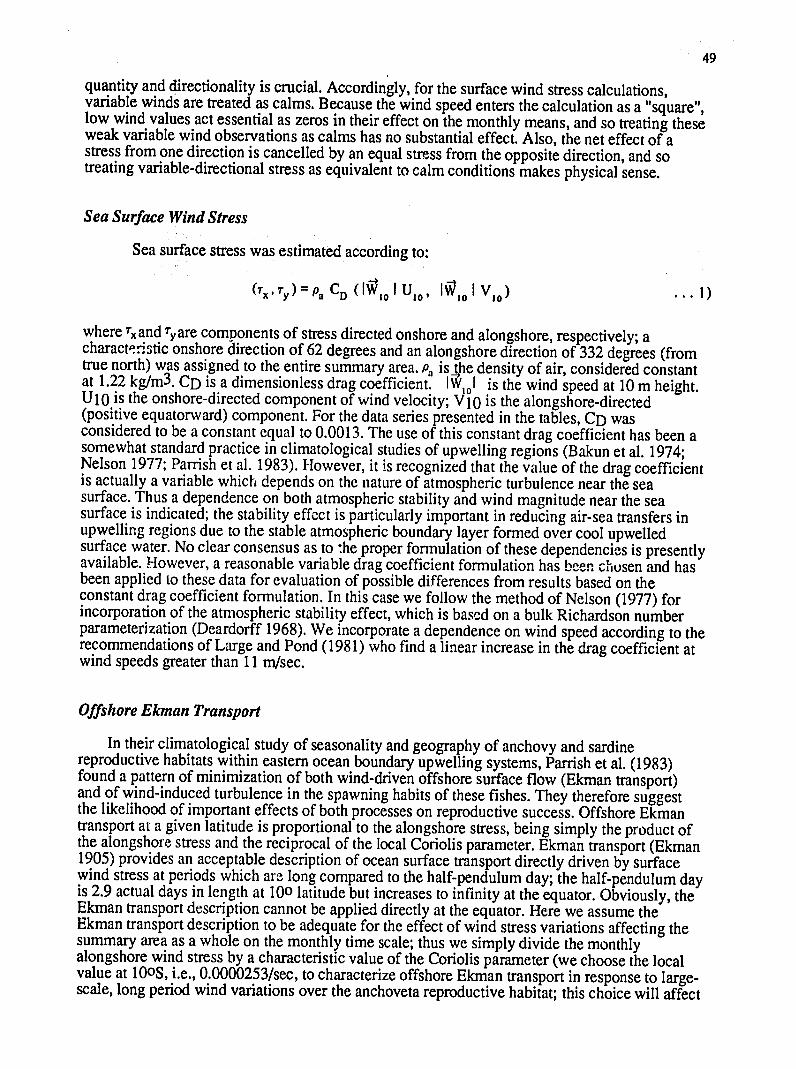
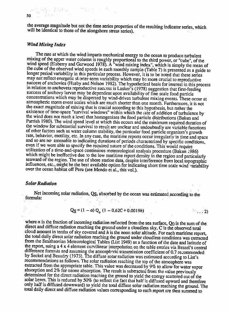
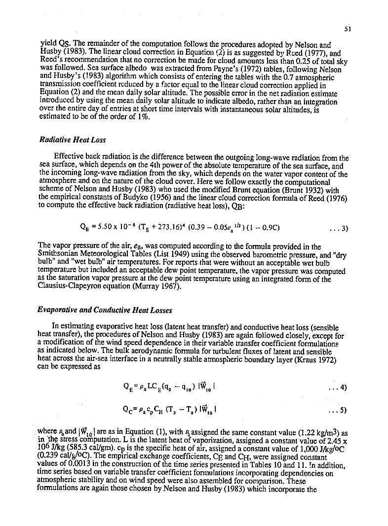
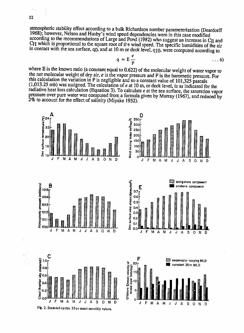
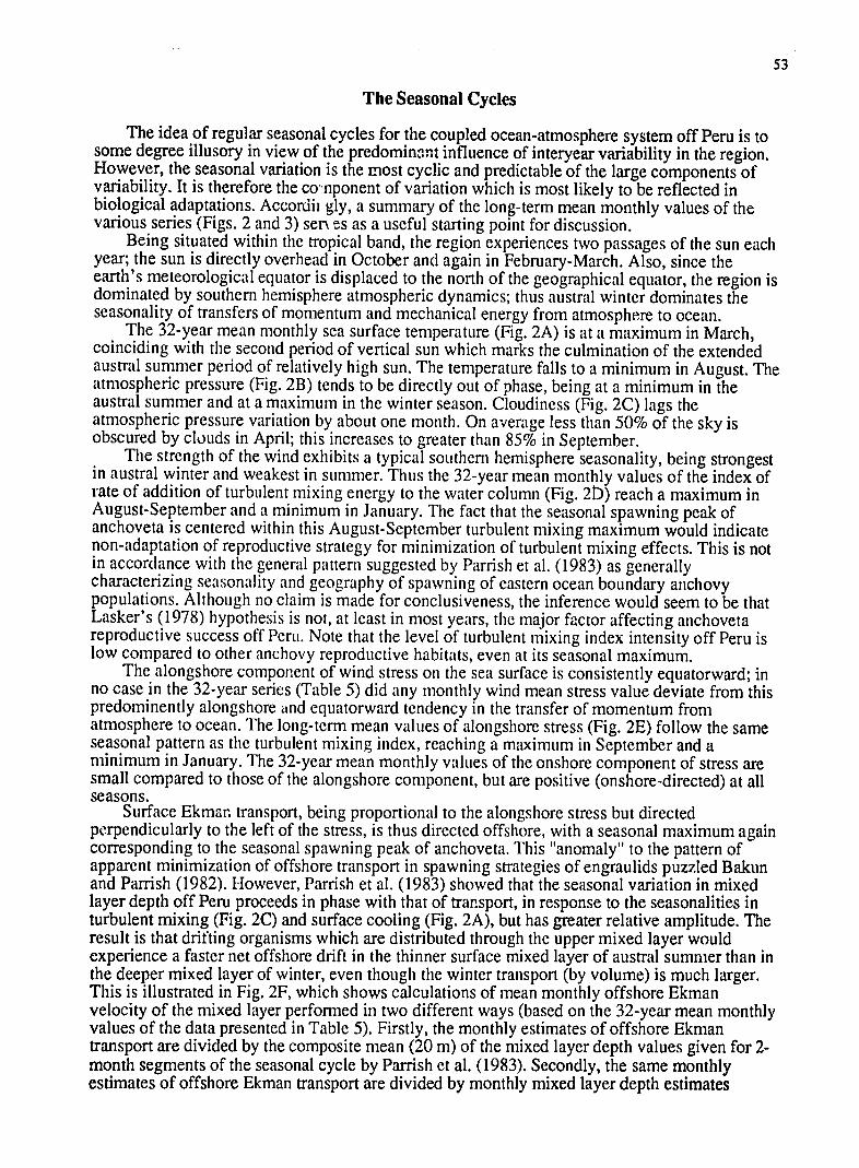
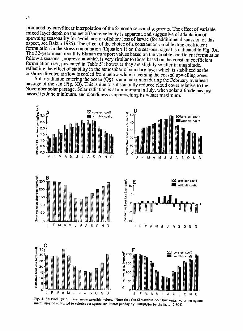
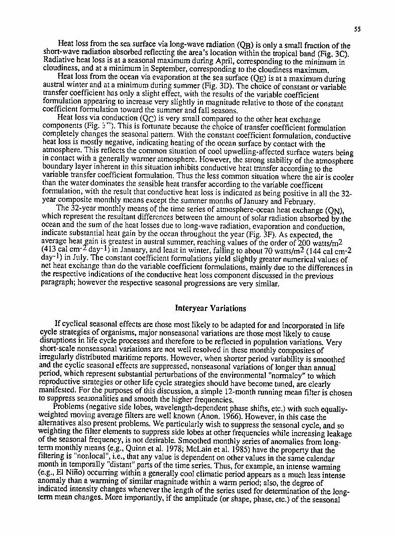
55
Heat loss from the sea surface via long-wave radiation (QB) is only a small fraction of theshort-wave radiation absorbed reflecting the areas location within the tropical band (Fig 3C)Radiative heat loss is at a seasonal maximum during April corresponding to the minimum incloudiness and at a minimum in September corresponding to the cloudiness maximum
Heat loss from the ocean via evaporation at the sea surface (QE) is at a maximum duringaustral winter and at a minimum during summer (Fig 3D) The choice of constant or variabletransfer coefficient has only a slight effect with the results of the variable coefficientformulation appearing to increase very slightly in magnitude relative to those of the constant coefficient formulation toward the summer and fall seasons
Heat loss via conduction (Qc) is very small compared to the other heat exchangecomponents (Fig 3) This is fortunate because the choice of transfer coefficient formulationcompletely changes the seasonal pattern With the constant coefficient formulation conductiveheat loss is mostly negative indicating heating of the ocean surface by contact with theatmosphere This reflects the common situation of cool upwelling-affected surface waters beingin contact with a generally warmer atmosphere However the strong stability of the atmosphereboundary layer inherent in this situation inhibits conductive heat transfer according to thevariable transfer coefficient formulation Thus the less common situation where the air is coolerthan the water dominates the sensible heat transfer according to the variable coefficentformulation with the result that conductive heat loss is indicated as being positive in all the 32shyyear composite monthly means except the summer months of January and February
The 32-year monthly means of the time series of atmosphere-ocean heat exchange (QN)which represent the resultant differences between the amount of solar radiation absorbed by the ocean and the sum of the heat losses due to long-wave radiation evaporation and conductionindicate substantial heat gain by the ocean throughout the year (Fig 3F) As expected the average heatgain is greatest in austral summer reaching values of the order of 200 wattsm2(413 cal cm-2 day-1) in January and least in winter falling to about 70 wattsm 2 (144 cal cm-2 day-i) in July The constant coefficient formulations yield slightly greater numerical values ofnet heat exchange than do the variable coefficient formulations mainly due to the differences inthe respective indications of the conductive heat loss component discussed in the previousparagraph however the respective seasonal progressions are very similar
Interyear Variations
If cyclical seasonal effects are those most likely to be adapted for and incorporated in lifecycle strategies of organisms major nonseasonal variations are those most likely to causedisruptions in life cycle processes and therefore to be reflected in population variations Veryshort-scale nonseasonal variations are not well resolved in these monthly composites ofirregularly distributed maritime reports However when shorter period variability is smoothedand the cyclic seasonal effects are suppressed nonseasonal variations of longer than annualperiod which -represent substantial perturbations of the environmental normalcy to whichreproductive strategies or other life cycle strategies should have become tuned are clearlymanifested For the purposes of this discussion a simple 12-month running mean filter is chosen to suppress sea sonalities and smooth the higher frequencies
Problems (negative side lobes wavelength-dependent phase shifts etc) with such equallyshyweighted moving average filters are well known (Anon 1966) However in this case thealternatives also present problems We particularly wish to suppress the seasonal cycle and soweighting the filter elements to suppress side lobes at other frequencies while increasing leakageof the seasonal frequency is not desirable Smoothed monthly series of anomalies from longshyterm monthly means (eg Quinn et al 1978 McLain et al 1985) have the property that thefiltering is nonlocal ie that any value is dependent on other values in the same calendarmonth in temporally distant parts of the time series Thus for example an intense warming(eg El Niiio) occurring within a generally cool climatic period appears as a much less intenseanomaly than a warming of similar magnitude within a warm period also the degree ofindicated intensity changes whenever the length of the series used for determination of the longshyterm mean changes More importantly if the amplitude (or shape phase etc) of the seasonal
56
variation is undergoing nonseasonal variation taking anomalies introduces spurious seasonalshyscale variations into the filtered series A local seasonal filter that avoids some of these problems can be based on 12th-differences eg the result of subtracting from each monthlyvalue the value for the same calendar month in the previous year but the result is therebytransformed to annual rates of change of a property rather than the property itself which complicates a descriptive discussion However the use of 12th-difference transforms is worth considering for empirical modelling efforts For the purposes of this discussion the simple 12shymonth running mean provides a local seasonal filtersmoother which will be familiar to manyreaders and adequate for a descriptive treatment
The filtered sea surface temperature series (Fig 4A) illustrates well the major El Niio warm events of the period 1957-1958 1965 1969 1972-1973 1976 and 1982-1983 Generallyelevated temperatures in the period between the 1976 and 1983 events are also apparent Also apparent is the extended cold period of the mid- 1950s the indication of rise in temperature from this cold period to the peak of the 1957-1983 El Niiio is comparable in total magnitude to that of the rise of the 1982-83 El Ni-io from the much warmer climatic base temperature level of the late 1970s
Major features in the filtered cloud cover series (Fig 4B) are visibly related to those in the temperature series but not in any simple consistent manner Cloud cover minima often appearto coincide with the relaxation of El Nifio events An extraordinarily low degree of cloudings appears to have coincided with the return to normal sea temperatures in 1984 Another sharpcloud cover minimum coincided with the leveling off of the temperature decline following the 1957-1958 event Likewise cloud cover maxima often appear to coincide with rapid drops of temperature into cool periods Atmospheric pressure variations (Fig 4C) are obviously highlyinversely correlated at these low frequencies with those of sea surface temperature
It is not surprising in view of the dynamic linkage of wind to horizontal gradient of atmospheric pressure that wind variations would be related to those of atmospheric pressureThe relation of the wind-cubed index of rate of addition of turbulent mixing energy to the ocean by the wind (Fig 4D) to El Nifio periods is striking El Niffo events are evidently strongwind-mixing events which according to Laskers (1978) scenario would correspond to periodsof high probability of starvation for first-feeding anchoveta larvae The period during and immediately following the 1972 El Nifio appears to have been characterized by an extended period of highly turbulent upper water column conditions The period during and following the 1982-1983 event appears to have been similarly turbulent except for a 2-month window of relaxed turbulent mixing index during December 1983 and January 1984 (somewhat masked bythe smoothing in Fig 4C but evident in the unsmoothed monthly values in Table 7)
The magnitude of alongshore (equatorward) wind stress also increases during El Nifio events (Fig 4E) in agreement with Wyrtkis (1975) conclusions which were based on a summary area displaced somewhat southward along the coast (10-200S 70-80oW) from the oneused here (Fig 1) Thus in addition to potential increases in larval starvation due to increased destruction of food particle strata by turbulent mixing an increase in potential offshore loss of larvae from the favorable coastal habitat is also indicated The onshore component of surface wind stress is relatively small and consistently positive (onshore-directed) in the filtered series
In the previous section the effect of seasonally-varying mixed layer depth on the offshore Ekman velocity of particles which are continually mixed through the upper mixed layer was discussed (ie in reference to Fig 2F) To investigate the effect on interyear time scales filtered time series of offshore Ekman velocity were calculated as in that section ie (i) assuming a constant MLD of 20 m and (ii) assuming a seasonally varying MLD derived from the values given by Parrish et al (1983) The result indicates that at least for the MLD values chosen the effect of seasonally-varying mixed layer depth is such as to substantially increase on average the rate of offshore movement of passive particles in the mixed layer If the effective mixed layerdepth is increased during El Nifio as would be expected both from the effect of the propagatingbaroclinic wave in deepening the surface layer and also from the enhanced wind induced turbulent mixing the effect would be to counteract the increased rate of offshore movement indicated from the Ekman transport calculations
The effect of the choice of constant or variable drag coefficient formulation in the stress computation (Equation 1)is illustrated in Fig 4G where the alongshore stress variation is
25 S24- 28
V)
21
is-1_
55
20
is-__var
60 65
Year
70 75 80
85
020-
---
-1612
-- shy
55
60 65
Year
70
tp
constant coefficientviable coefficient
75 80
-
85
B H
1220 -
- -681 oW210
60
55
56
60 65 Yea
70 75
80
)
85
2 20
u ~190 55 60 65
Year 70
75
80 s
-
85
10135-
13
E10120shy
30
10125-a
010o 55 60 65
Year 70 75 80 85
22
Year
Fig 4 Low-frquency nonseasonal variations 12-month running means of monthly time series values (Note that the SI-standard heat flux units watts per square meter may be converted to calories per square centimeter per day by multiplying by the factor 2064)
-t-4
Ln
D
iso- 80constant 70
coefficientshyvariable coefficient
200
040
B-30 -20shy
55 60 65 Y aYear 80 85 55 60 65 Ya 70 75 80 85
E K
5
Eon~shor
C- 2
tol_
lonshore com ponent copnn --
ID
ISO
160
is 140
12D
I
I00
constant coefficient -
variable coefficient
-
55 60 65 70 75
YeauirY e a r
80 85
~ ~iii~
55 60 65 70
Year -Y 008
75 85
mnl mean lnaitude
2ee e pe ue c pe d by mliyn h factor52064)81b
- seasonally-varying MID ----- e 795 55
6 -
60 0
65 775 80 85 55 60 1 IIl5 I
65 7075 08 Y e ar YYore a -
Fig 4 Continued Low-frequency nonseasonal varitions 12-month running -neans of monthly time series values (Note that the Sl-standard heat flux units watts per square meter may be converted to calories per square centimeter perday by multiplying by the factor 2064)
59
plotted in terms of its directly proportional transform offshore Ekman transport The variable coefficient formulation produces generally lower estimates of stress due to the influence of the stability of the lower atmospheric boundary layer over upwelling-affected surface waters However the differences essentially disappear during the period of relaxation of the intense El Niios of 1957-1958 and 1982-1983 A possible explanation is the tendency for a less stable atmosphere in contact with the ocean surface due to residual warmth which would linger longerin the ocean than in the atmosphere due to the much greater heat storage capacity of water compared to that of air
The filtered series of estimates of absorption of solar radiation by the ocean (QS) exhibits some interesting patterns (Fig 4H) Since the variables that control the solar radiation estimate (Equation 2) derived from a maritime report at any given latitude are calendar date and cloud cover it is not surprising that maxima in Fig 4H often correspond to minima in Fig 4B and vice versa However there are discernible differences between the two series that result from the interaction of the cloud cover variations with the seasonal changes in solar height in the solar radiation time series An impressive feature in the solar radiation series is the early largeshyamplitude alternation consisting of deep minimum of solar radiation entering the ocean corresponding to the early part of the intense 1954-1955 cold period followed by a sharp highlyerratic rise to a high peak in early 1960 In addition the entire period of the 1960s and the first half of the 1970s appears to have been characterized by low absorption of solar radiation relative to the more recent period since 1976
The long-wave radiative heat loss (QB) tends to be an order of magnitude smaller than the short-wave absorption but varies very similarly (Fig 41) This similarity is perhaps explainablein the similar dependence of both types of estimate on cloud cover with the sea surface temperature dependence in the long-wave radiation estimate (Equation 3) being related seasonally to the solar height dependence in the solar radiation estimate (Equation 2) There mayalso be some actual causal effect of the long period variations in solar radiation on the sea temperature dependence in the long-wave radiation estimate
The filtered series of evaporative heat loss (QE) delineates the various El Niffo episodes and the 1954-1955 cold period in a very similar fashion to the sea surface temperature series (Fig4J) The long-term variation in vapor pressure difference between the sea surface and the overlying atmosphere (Equation 4) is apparently very closely linked to that of sea surface temperature As discussed above the wind speed dependence is also a strong function of these climate scale events The effect of choice of constant or variable transfer coefficient apparentlymakes very little difference except during the mid-1950s cold period where increased stability of the air over the cold ocean apparently inhibited the turbulent exchange of latent heat according to the variable coefficient formulation
The net ocean-atmosphere heat exchange series (QN) indicates long-term variations in net ocean heat gain such that minima are associated with El Nifio episodes and maxima with cold periods The variations appear to be controlled to a substantial extent by the evaporative heat loss (Fig 4J) This is so because the variations in heat gain by absorption of short-wave solar radiation (Fig4H) are partially offset by the highly correlated variations in long-wave radiative heat loss (Fig 41) The net effect of the choice of variable or constant transfer coefficient formulations in the evaporative and conductive components is a slight general lowering of the magnitude oi net heat gain in the variable coefficient case This difference is due primarily to the stability effect on the conductive heat loss term as discussed in the previous section in reference to Fig 2E where the average change in the mean net value of this component approximately 5 wattsm2 corresponds in general to the approximate difference between the curves in Fig 4K except in the mid-1950s where stability effects on the evaporative heat loss term are appreciable
In order to check for long-period variations in the distribution of observations within the summary area (Fig 1) filtered series of the monthly averages of the respective latitudinal and longitudinal locations of reports were prepared (Fig 4L) Since the coastline is oriented somewhat northwest to southeast variations in the two curves which tend tc parallel each other in the figure will tend to yield a resultant displacement in the alongshore direction More serious with respect to the long-term homogeneity of the monthly series herein presented are variations in Fig 4L where the curves are changing in the opposite sense ie where the net displacement of the mean position of reports is in the onshore-offshore direction these situations are
60
Table 1 Numbers of observations in monthly samples used to construct timeseries For each month the first number refers to observations used in constructing the values in Tables 2456 amp 7 (sea temperature atmosphericpressure wind stress components and wind cubed index the 2nd number refers to observations used in constructing the values in Table 4 (cloudcover) the 3rd number refers to observations used for values in Tables 8910 amp 11 (heat exchange components)
Jan Feb Mar Apr May Jun1953 21 19 191 29 29 291 22 22 191 23 23 101 33 33 331 16 16 61954 61 57 40 19 19 171 21 21 211 59 59 531 42 39 391 36 34 24 1955 24 22 201 35 35 291 16 15 121 9 9 51 24 24 13 35 35 301956 - 41 38 151 17 15 151 16 16 31 39 39 211 22 22 161 20 20 71957 32 32 321 25 24 151 98 98 471 38 38 291 25 25 211 53 52 33 1958 153 153 1061 74 73 441 69 69 341 84 84 281 67 66 441110 107 521959 128 125 511162 162 491143 138 371115 112 371 97 96 211 67 67 43 1960 98 95 421148 146 1101166 166 1051151 146 1011171 164 1351 85 82 591961 148 147 1271124 124 901115 111 941183 180 1501 89 86 661130 128 1041962 185 183 1271149 148 1341163 162 1421157 155 1221114 111 1051177 177 147 1963 78 76 711103 102 1021182 181 1671180 177 1701157 156 1491185 185 1851964 129 12S 981138 137 1351 82 81 811 76 76 761 45 45 451 52 52 521965 59 59 581 75 71 701137 137 1371 99 99 961139 136 1361139 139 1381966 107 107 1071 82 82 821113 112 1111106 106 1061117 113 1101137 137 137 1967 111 109 1021 60 52 521 80 80 781147 144 1441 75 74 741 66 66 661968 76 76 761128 127 1271108 108 1081139 137 1371 91 87 871111 109 1081969 67 67 67 87 84 841134 131 1311 91 91 911 56 56 561102 102 102 1970 90 87 821 57 57 531103 100 901 51 51 481 99 98 921208 206 200 1971 103 101 931 81 77 751 89 89 891 53 53 521 44 44 441 22 22 211972 109 108 1041 54 52 511 49 49 471 85 85 851 81 81 811 56 56 561973 55 54 401 44 44 391 89 89 891 50 50 481 58 58 561 57 54 471974 84 78 781 63 63 581113 109 1001 57 54 541119 118 1171 73 72 721975 59 57 561 73 72 691140 140 1401 99 92 901140 138 1361116 115 114 1976 70 69 681 20 19 191 76 73 711 59 59 551 71 71 701 49 44 401977 51 51 511109 106 1051 79 79 731101 99 941 93 88 871 70 70 69 1978 57 56 561 65 65 621 71 69 671 92 92 881 71 71 711 41 40 35 1979 97 96 89 58 57 511105 104 981 85 85 771 83 80 741 48 45 341980 96 93 801106 105 931125 123 1021 75 70 541151 146 1191246 201 98 1981 116 113 851 90 89 821139 137 1241108 103 951115 108 791128 124 1081982 91 89 821 90 90 801152 146 1391100 98 881103 98 801 54 54 41 1983 68 64 541126 126 1161 94 91 861 76 72 611 93 92 831 61 61 551984 90 75 261 99 80 391 90 59 141 75 41 161 58 39 61 56 49 29
Jul Aug Sep Oct Nov Dec 1953 10 10 91 39 35 261 29 28 251 18 18 11 24 24 181 19 18 111954 40 39 381 14 14 101 27 26 221 43 371 30 30 61 18 18 9 1955 17 17 121 37 36 211 35 35 61 45 44 341 27 27 201 13 13 51956 45 45 361 21 21 211 29 29 211 41 40 291 63 61 201 24 24 61957 27 27 111 24 24 211 64 64 381112 110 651100 99 531115 115 86 1958 51 51 271159 159 831 96 93 441113 108 471115 110 631 58 43 26 1959 100 100 571103 101 391 85 81 421 74 74 211110 110 551114 114 85 1960 169 168 1471114 111 671142 142 941 75 75 461 63 63 231 82 81 591961 108 107 821155 155 1421153 151 1411128 127 801197 197 1921135 133 118 1962 213 212 1931168 168 1591 81 81 751129 125 1251173 172 1521 91 88 791963 120 120 1201 70 70 701110 110 l011 70 70 701 61 61 581 56 56 53 1964 90 88 871 71 65 641 94 94 881129 127 1211 62 61 581105 104 1021965 92 92 921119 117 1151 99 99 981 67 67 671177 176 1761111 Ill 1061966 116 112 1121122 118 1181185 182 1821131 125 1251 89 89 881123 123 123 1967 89 87 871 67 67 671 84 84 841 76 71 711 73 73 731 99 97 971968 58 58 581 82 81 811 59 59 561111 109 1081118 118 1181 66 65 65 1969 70 70 701 86 84 841108 97 921102 102 971137 137 1271101 101 96 1970 75 74 741 66 65 651 91 90 901 50 50 501127 125 1241 68 68 671971 43 43 421 58 58 541 28 28 231 51 51 471 78 78 781 34 31 30 1972 35 32 301 60 58 541 32 32 291 81 74 741 31 28 261 51 51 48 1973 81 75 741105 92 881 89 84 821 55 54 501100 98 981 71 71 701974 102 101 1011 90 89 891 67 66 661 53 52 501 78 78 771 44 44 441975 67 66 651 53 48 471 70 68 681 70 65 601 68 68 671 88 88 88 1976 74 74 721 21 21 181 88 87 861 76 76 731 46 44 441 58 57 57 1977 55 54 531 55 51 511 73 70 681106 104 1041183 166 1631 67 59 31978 37 33 301 5T S1 501 73 72 671 53 49 491 99 79 761 87 87 851979 80 75 631137 108 q01116 109 821 84 77 531 77 75 591 39 35 26 1980 281 233 53j2tj7 182 9CI148 131 941129 118 891 80 74 611 70 66 471981 169 161 781174 159 631122 111 921127 115 971174 155 1421154 147 127 1982 78 74 681 78 70 661 71 62 551106 102 811132 124 1131 93 89 511983 124 121 841145 116 4F1 70 48 191156 150 901 73 73 241 96 90 321984 104 90 411113 87 81 75 --54 14195 51 69 251 62 40 77 61 35
61
Table 2 Sea surface temperature in degrees Celsius The standard error of the mean appears within parentheses to the right of the mean temperaturevalue
Jan Feb Mar Ap May Jun 1953 2114(50) 2308(64) 2463(51) 2478(49) 2279(37) 2052(46) 1954 1855(33) 2286(46) 2201(42) 1636(29) 1786(23) 1695(25) 1955 2172(39) 1850(52) 2101(85) 1901(37) 1789(85) 1667(30) 1956 1990(44) 1764(82) 2166(46) 2071(29) 1990(41) 1922(29) 1957 1947(47) 2483(48) 2526(21) 2453(37) 2476(48) 2315(27) 1958 2315(11) 2500(19) 2452(25) 2283(30) 2163(35) 2042(18) 1959 2045(21) 2308(18) 2449(15) 2154(25) 2090(18) 1926(25) 1960 2197(18) 2274(18) 2270(19) 2058(18) 1909(14) 1822(18) 1961 2230(15) 2324(20) 2161(21) 1994(15) 2024(21) 1867(15) 1962 2129(14) 2212(18) 2037(18) 1941(18) 1868(18) 1892(12) 1963 2072(24) 2267(17) 2215(16) 2021(17) 2101(13) 1898(10) 1964 2144(12) 2241(14) 2091(22) 2066(37) 1838(26) 1735(24) 1965 2175(26) 2309(27) 2396(15) 2454(21) 2408(20) 2211(14) 1966 2209(20) 2362(20) 2196(25) 2085(24) 1988(24) 1867(16) 1967 2002(22) 2212(22) 2186(23) 2061(19) 1911(24) 1813(30)
1968 1967(21) 2221(21) 2178(22) 1860(20) 1849(30) 1731(20) 1969 2228(23) 2236(23) 2425(18) 2351(23) 2294(25) 2092(22) 1970 2171(26) 2194(43) 2251(26) 2040(33) 1873(21) 1685(14) 1971 1970(19) 2034(29) 1970(25) 2163(36) 1980(32) 1846(46) 1972 2094(25) 2438(41) 2517(37) 2297(24) 23U5(22) 2168(24) 1973 2422(25) 2440(39) 2252(20) 1954(31) 1916(37) 1736(35) 1974 2072(30) 2200(36) 2210(31) 2135(36) 2136(24) 1951(19) 1975 2125(28) 2241(24) 2341(19) 2221(27) 2081(21) 1867(18) 1976 2116(30) 2338(64) 2296(33) 2245(35) 2164(28) 2123(30) 1977 2369(22) 2346(19) 2244(32) 2044(28) 1977(24) 1966(27) 1978 2106(24) 2346(25) 2257(25) 2269(32) 2007(34) 1995(49) 1979 2242(19) 2311(28) 2362(22) 2271(26) 2037(31) 2061(45) 1980 2169(25) 2322(21) 2421(21) 2248(29) 2181(17) 2084(13) 1981 2090(26) 2280(22) 2210(24) 2099(28) 2073(20) 1944(16) 1982 2133(22) 2262(30) 2165(23) 2120(24) 2101(22) 2115(41) 1983 2642(19) 2738(19) 2799(14) 2793(20) 2772(15) 2593(30) 1984 2213(221 2278(291 2192(261 2095(33) 1917(31) 1949f281
Jul Aug Sep Oct Nov Dec 1953 1978(27) 1906(21) 1820(34) 1824(35) 1872(40) 1881(41) 1954 1460(35) 1557(41) 1491(31) 1422(29) 1711(26) 1924(54) 1955 1768(53) 1554(45) 1571(28) 1469(37) 1709(24) 1812(37) 1956 1694(24) 1765(37) 1748(29) 1675(19) 1838(29) 1923(40) 1957 2243(34) 1928(34) 1894(19) 1923(17) 1907(16) 2075(16) 1958 1963(26) 1737(10) 1780(15) 1790(13) 1898(18) 2025(31) 1959 1755(15) 1680(12) 1664(18) 1777(20) 1904(20) 1935(15) 1960 1765(10) 1742(12) 1717(11) 1753(18) 1878(24) 2059(17) 1961 1004(22) 1762(11) 1687(11) 1736(16) 1854(14) 1939(17) 1962 1730(09) 1727(10) 1677(10) 1689(10) 1808(12) 1949(21) 1963 1870(13) 1824(17) 1800(11) 1755(16) 1854(28) 1972(17) 1964 1710(18) 1611(20) 1611(14) 1640(15) 1831(32) 1976(19) 1965 2059(20) 2000(20) 1779(16) 1826(23) 1876(13) 2149(15) 1966 1800(12) 1675(13) 1681(10) 1737(12) 1813(17) 1977(20) 1967 1740(16) 1646(17) 1S76(13) 1609(21) 1690(18) 1822(21) 1968 1764(23) 1705(17) 1826(38) 1765(17) 1767(16) 2082(24) 1969 1844(20) 1801(17) 1736(19) 1824(16) 1839(13) 1949(15) 1970 1572(12) 1619(13) 1633(28) 1636(25) 1794(16) 1829(21) 1971 2800(28) 1727(23) 1632(26) 1705(27) 1834(15) 1981(35) 1972 2118(36) 2177(23) 1929(36) 1917(35) 2061(32) 2173(31) 1973 1688(32) 1604(16) 1580(22) 1611(31) 1727(24) 1901(30) 1974 1812(15) 1748(15) 1670(31) 1691(32) 1896(23) 1983(35) 1975 1846(25) 1768(36) 1571(24) 1559(20) 1624(15) 1874(24) 1976 2118(20) 1951(55) 1900(23) 1919(25) 2004(23) 2146(15) 1977 1854(25) 1723(22) 1721(28) 1849(28) 1895(16) 1945(24) 1978 1849(35) 1691(33) 1727(25) 1811(25) 1940(30) 2049(24) 1979 1873(25) 1830(26) 1901(28) 1853(23) 1925(27) 2104(38) 1980 2004(11) 1835(13) 1777(15) 1839(23) 1895(27) 2021(21) 1961 1808(17) 1824(11) 1767(24) 1786(23) 1898(15) 2029(15) 1982 1965(18) 1834(23) 1900(36) 2061(22) 2303(17) 2519(21) 1983 2324(23) 2126(21) 1957(25) 1989(14) 2025(22) 2154(27) 1984 1952(231 1837(131 1844(18) 1827(281 1970(311 2020(311
62
Table 3 Total cloud amount Valvas indicate mean fraction of sky obscuredThe standard error of the mean appaars in parentheses to the right of each mean value
Jan Feb Mar ApM May1953 66(06) s8(06) 43(06) 43(08) 54(06)
Jun 76(10)1954 59(05) 75(05) 69(07) 35(04) 85(05) 74(07)1955 55(07) 61(06) 60(09) 06(04) 69(08) 90(04)1956 66(05) 46(l0) 40(06) 33(06) 65(08) 89(06)
1957 48(07) o(05) 56(03) 57(05) 5(06) 76(04)1958 60(03) 68(03) 63(03) 32(04) 54(04) 83(03)1959 40(03) 58(C2) 66(02) 60(03) 83(03) 78(04)1960 so(03) 30(03) 38(02) 44(03) 52(03) 63(05)1961 65(03) 44(03) 65(03) 50(03) 49(04) 79(03)1962 55(02) 54(03) 48(03) 56(03) 53(04) 79(03)1963 50(04) 52(03) 61(02) 52(03) 66(03) 81(02)1964 64(03) 66(03) 57(04) 51(04) 72(06) 63(06)1965 54(04) 49(04) 61(02) 60(03) 63(03) 64(03)1966 56(03) 44(03) 57(03) 45(03) 62(03) 76(03)1967 72(03) 51(05) 56(03) 51(03) 46(04) 82(04)1968 52(04) 52(03) 45(03) 38(03) 65(04) 75(03)1969 57(04) 55(04) 58(03) 57(04) 70(05) 81(03)1970 59(04) 43(04) 37(03) 43(05) 62(04) 81(02)1971 51(03) 3s(04) 48(03) 52(05) 68(06) 8s(06)1972 53(04) 49(04) 64(03) 53(04) 69(04) 78(04)1973 67(03) 61(05) 60(04) 49(04) 40(05) 70(05)1974 59(03) 52(04) 53(03) 53(05) 77(03) 8(02)1975 69(04) 50(04) 60(02) 54(03) 72(03) 86(03)1976 61(04) 59(08) 63(03) 55(05) 62(04) 87(04)1977 54(05) 68(03) 55(04) 34(03) 53(04) 71(04)1978 53(04) 65(04) 45(04) 57(04) 54(05) 68(07)1979 s0(03) 53(04) 56(03) 44(03) 67(04) 79(05)1980 57(03) 53(03) 58(03) 48(04) 57(03) 80(02)1981 66(03) 63(03) 51(03) 57(03) 66(03)1982 80(03)
60(03) 58(03) 55(03) 52(03) 58(04) 84(04)1983 52(04) 47(02) 63(03) 70(03) 75(03) 74(04)1984 42(041 43(031 45(03) 40(04) 34(051 74(041
Jul Aug SeD Oct NOV Dec1953 65(14) 91(04) 74(07) 74(07) 81(06) 67(07)1954 79(05) 86(07) 92(05) 89(04) 72(05) 75(08)1955 97(02) 90(04) 90(04) 80(05) 61(08) 44(10)1956 85(05) 82(08) 64(05) 62(05) 73(05) 49(08)1957 79(06) 72(08) 85(04) 72(03) 72(03) 64(03)1958 79(05) 80(03) 90(02) 81(03) 52(04) 45(06)1959 78(03) 78(03) 79(04) 79(03) 63(04) 51(03)1960 72(03) 81(03) 90(02) 89(03) 63(05) 67(04)1961 94(01) 83(02) 90(02) 78(03) 61(02) 60(03)1962 90(02) 93(02) 86(03) 88(02) 77(02) 46(04)1963 80(03) 80(04) 88(02) 82(04) 77(04) 68(05)1964 87(03) 87(03) 86(03) 88(02) 77(04) 51(03)1965 88(03) 90(02) 92(02) 86(03) 75(02) 61(03)1966 77(03) 83(03) 85(02) 89(02) 83(03) 61(03)1967 88(03) 91(03) 84(03) 85(04) 86(03) 47(04)1968 80(05) 93(02) 88(03) 83(03) 76(03)1969 86(04) 83103) 91(02) 82(03) 68(03) 50(04)
56(04) 1970 87(04) 91(03) 85(03) 95(02) 59(03) 64(04)1971 94(02) 88(03) 92(03) 853(05) 65(04) 65(06)1972 83(05) 80(04) 87(04) 78(04) 86(05) 67(05)1973 82(03) 91(02) 87(03) 80(04) 81(03) 72(04)1974 91(02) 89(03) 88(03) 75(05) 72(04) 57(05)1975 86(03) 89(03) 89(03) 77(04) 78(04) 64(04)1976 80(04) 93(03) 77(03) 81(03) 78(04) 53(04)1977 89(03) 86(04) 83(04) 81(03) 72(02) 41(05)1978 9s(0l) 84(04) 80(104) 8l(04) 68(04) 50(03)1979 865(03) 8l(03) 83(03) 8(03) 8o(03) 49(06)1980 90(01) 90(02) 81(02) 82(02) 69(04) 48(04)1981 87(02) 83(02) 92(02) 67(03) 63(03) 51(03)1982 80(04) 88(03) 82(03) 76(03) 75(03) 58(03)1983 72(03) 68(03) 66(06) 80(02) 58(04) 49(04)1984 81(031 75(031 86(031 91(03 70o051 52(041
63
Table 4 Atmospheric pressure at sea level Add 10000 to the mean valuesin the table to yield pressure in millibars The standard error of the mean appears in parentheses to the right of each mean value the standard errors are given (directly) in millibars
Jan Feb Mar A r May Jun1951J 112( 3) 104( 1) 111( 3) 132( 5) 125( 2) 145( 5)1954 123( 2) 122( 4) 102( 4) 213( 3) 135( 3) 147( 3)1955 125( 3) 109( 2) 104( 4) 119( 5) 136( 2) 152( 2)1956 115( 2) 107( 4) 111( 3) 109( 3) 120( 2) l0O( 6)1957 128( 2) 86( 3) 109( 3) 99( 3) 123( 2) 123( 2)1958 219( 2) 115( 2) 72( 4) 98( 3) 115( 2) 132( 1)1959 120( 2) 109( 1) 115( 2) 112( 1) 133( 2) 142( 2)1960 116( 2) 215( 2) 113( 2) 115( 1) 127( 1) 137( 2)1961 106( 4) 106( 2) 106( 2) 112( 4) 129( 1) 136( 2)1962 130( 1) 118( 2) 120( 1) 128( 2) 140( 2) 153( 1)1963 129( 2) 136( 2) 112( 1) 135( 4) 132( 1) 142( 1)1964 23( 1) 105( 1) 112( 2) 122( 2) 127( 4) 142( 2)1965 117( 1) 102( 2) 110( 2) 115( 1) 113( 2) 129( 2)1966 106( 2) 102( 2) 202( 1) 118( 2) 132( 1) 146( 1)1967 115( 2) 123( 2) 120( 2) 113( 2) 131( 2) 143( 2)1968 113( 2) 117( 1) 126( 2) 129( 1) 143( 2) 156( 1)1969 112( 3) 96( 1) 114( 2) 113( 1) 115( 2) 13s( 2)1970 128( 2) 110( 2) 118( 1) 117( 2) 145( 2) 144( 1)1971 119( 2) 108( 2) 108( 2) 123( 2) 138( 3) 153( o4)1972 109( 2) 210( 3) 103( 2) 115( 2) 118( 2) 121( 2)1973 105( 4) 118( 2) 107( 2) 115( 3) 130( 3) 145( 2)1974 119( 5) 118( 2) 125( 2) 126( 3) 137( 3) 142( 2)1975 115( 3) 119( 2) 114( 1) 119( 2) 135( 1) 140( 1)1976 121( 3) 116( 7) 106( 1) 119( 2) 125( 2) 120( 2)1977 204( 3) 212( 1) 100( 2) 120( 4) 126( 2) 137( 2)1978 139( 3) 101( 7) 120( 2) 123( 2) 128( 2) 150( 3)1979 122( 1) 119( 3) 114( 2) 110( 3) 133( 3) 155( 5)1980 129( 2) 123( 2) 93( 2) 105( 2) 129( 2) 145( 3)1981 139( 3) 108( 2) 114( 2) 121( 2) 143( 2) 18( 4)1982 126( 5) 114( 2) 104( 2) 121( 2) 126( 2) 129( 3)1983 91( 3) 97( 2) 91( 2) 95( 2) 96( 3) 116( 2)1984 125(21 107( 3) 107( 51 131f 3 137( 7) 139( 21 1953 137( 5) 134( 2) 130( 2) 150( 5) 140( 3) 132( 4)1954 138( 3) 143( 4) 138( 3) 148( 2) 145( 2) 130( 3)1955 157( 3) 151( 3) 154( 3) 161( 3) 140( 2) 131( 5)1956 149( 3) 137( 4) 144( 3) 141( 2) 142( 5) 94( 6)1957 130( 3) 140( 3) 125( 3) 134( 2) 128( 2) 122( 2)1958 141( 3) 139( 2) 140( 3) 127( 2) 128( 2) 106(l7)2959 136( 1) 141( 2) 131( 2) 137( 2) 133( 2) 122( 3)1960 145( 1) 145( 2) 141( 1) 140( 2) 111( 2 135( 3)1961 144( 2) 144( 1) 147( 1) 13b( 1) 147( 2) 132( 1)1962 144( 1) 152( 2) 139( 3) 153( 2) 106(14) 138( 2)1963 143( 2) 136( 3) 138( 4) 144( 1) 154( 4) 124( 2)1964 148( 1) 148( 2) 142( 2) 143( 2) 131( 2) 132( 1)1965 126( 2) 140( 2) 141( 2) 139( 2) 121( 2) 116( 1)1966 140( 1) 149( 1) 148( 1) 141( 2) 136( 2) 123( 1)1967 142( 2) 145( 2) 152( 2) 140( 2) 134( 2) 130( 2)1968 148( 2) 152( 1) 140( 3) 135( 2) 141( 1) 126( 2)1969 143( 2) 149( 2) 130( 1) 138( 1) 132( 2) 122( 1)2970 155( 1) 144( 2) 138( 2) 139( 3) 139( 1) 110( 2)2971 137( 3) 143( 7) 145( 4) 153( 2) 140( 1) 123( 3)1972 125( 6) 128( 3) 129( 3) 131( 2) 122( 3) 218( 6)1973 147( 4) 148( 2) 152( 3) 151( 2) 143( 2) 148( 2)1974 138( 4) 147( 2) 149( 2) 140( 2) 137( 1) 126( 2)1975 152( 2) 151( 3) 155( 2) 153( 2) 151( 2) 135( 2)1976 133( 2) 146( 6) 133( 4) 137( 3) 139( 2) 104( 2)1977 135( 3) 143( 2) 147( 2) 142( 2) 137( 2) 124( 2)1978 139( 4) 141( 2) 145( 2) 138( 2) 123( 2) 123( 2)1979 149( 2) 142( 3) 147( 3) 148( 2) 141( 3) 125( 9)1980 151( 2) 152( 2) 141( 4) 138( 3) 138( 2) 137( 5)1981 150( 3) 160( 2) 148( 2) 139( 2) 134( 2) 119( 1)1982 120( 2) 129( 2) 141( 3) 129( 2) 106( 2) 100( 2)1983 118( 2) 142( 4) 150( 5) 136( 2) 133( 7) 142( 4)1984 126( 4 153( 31 148( 51 145( 31 142( 11 118( 31
64
Table 5 Alongshore component (positive equatorward) of wind stress on the sea surface Units are dynes per square centimeter The standard error of the mean appears in parentheses to the right of the mean alongshore stress valueValues in this table multiplied by the factor 395 (see text) yield offshoreBkma transport in cubic meters per second across each meter width
Jan FeP Mar A P May Jun 1953 36(06) 32(05) 44(07) 99(20) 83(09) 37(10)1954 24(03) 41(14) 10(02) 46(05) 56(08) 46(08) 1955 40(09) 16(03) 53(18) 18(08) 63(11) 45(09)1956 16(02) 25(07) 67(10) 83(09) 85(13) 50(05)29S 31(06) 53(21) 76(05) 86(10) 57(06) 76(07) 1958 40(05) 42(05) 45(05) 61(06) 57(07) 46(04)1959 34(03) 28(02) 40(03) 42(04) 30(03) 59(07)1960 23(03) 27(02) 41(03) 49(04) 53(09) 45(04)1962 20(02) 27(03) 39(04) 48(03) 70(06) 48(05)1962 42(02) 34(03) 47(03) 52(04) 51(04) 60(04)1963 32(04) 39(03) 61(03) 47(03) 59(04) 33(03)1964 49(04) 44(03) 51(05) 71(07) 63(07) 58(12)1965 29(04) 40(05) 40(03) 53(06) 97(07) 58(04)1966 60(04) 61(06) 46(04) 75(06) 59(05) 62(04)2967 40(04) 36(04) 29(03) 30(03) 37(04) 71(10)1968 15(02) 40(05) 36(03) 36(03) 34(05) 65(05)1969 29(04) 26(04) 47(04) 56(04) 45(07) 89(08)1970 33(04) 16(05) 40(05) 56(06) 55(05) 52(04)2971 17(04) 36(04) 34(03) 59(08) 43(07) 73(23)1972 29(03) 34(04) 56(11) 55(04) 42(04) 67(08)1973 57(06) 38(05) 73(05) 60(08) 67(11) 51(07)1974 32(04) 42(05) 48(04) 68(07) 71(05) 66(07)1975 40(04) 35(04) 72(05) 63(05) 74(04) 63(06)1976 21(04) 17(04) l(05) 77(07) 72(07) 56(08)1977 32(06) 56(06) 38(04) 57(05) 47(05) 67(05)1978 37(05) 47(06) 62(07) 71(08) 59(07) 72(12)2979 49(05) 54(09) 54(04) 68(05) 69(07) 92(14)1980 44(04) 47(05) 49(04) 49(05) 89(07) 58(03)2981 52(04) 30(03) 46(04) 54(04) 53(05) 84(08)1982 35(04) 47(04) 63(04) 55(04) 65(06) 91(12)1983 69(06) 66(04) 46(05) 74(08) 75(06) 107(09) 1984 26(041 53(111 80(131 31(11) 83(181 07(131
Jul Aug See Oct No Dec 1953 70(22) 36(05) 46(06) 53(08) 62(08) 27(05)1954 52(07) 89(21) 83(09) 24(02) 30(04) 20(04)1955 46(09) 88(14) 66(10) 65(12) 60(08) l1(04)1956 69(09) 52(13) 64(05) 50(C8) 45(04) 45(08) 2957 101(11) 54(08) 75(07) 56(06) 44(04) 56(04)2958 51(05) 71(06) 49(04) 43(04) 26(03) 39(05)1959 38(04) 53(04) 48(07) 44(05) 31(03) 23(03)1960 59(05) 55(04) 51(04) 48(06) 34(03) 36(04)1961 67(06) 50(04) 50(04) 40(03) 38(02) 31(03)1962 60(04) 49(04) 60(06) 49(04) 51(04) 23(02)1963 54(05) 48(06) 72(05) 72(11) 53(06) 36(04)1964 62(05) 71(09) 73(08) 57(04) 36(05) 42(04)1965 63(05) 84(07) 87(07) 60(07) 49(03) 49(04)1966 76(04) 74(06) 59(03) 52(04) 26(03) 26(02)1967 54(05) 72(07) 74(09) 73(09) 46(05) 35(06)1968 90(10) 72(08) 64(08) 59(03) 51(03) 62(08)1969 53(06) 71(08) 59(05) 42(04) 28(03) 37(04)1970 1971
47(06) 52(05) 45(04) 50(07) 41(03) 27(05)40(08) 77(112) 64(12) 71(08) 43(05) 49(09) 1972 90(11) 81(10) 132(19) 49(05) 35(04) 72(15)1973 70(11) 116(12) 101(11) 71(09) 58(05) 37(06)2974 73(05) 64(08) 72(07) 67(07) 68(05) 45(06)1975 64(07) 91(10) 73(05) 51(05) 36(04) 35(05)1976 59(05) 69(16) 80(06) 67(06) 64(06) 52(06)1977 94(11) 83(10) 47(06) 46(04) 157(04) 55(o06) 1978 87(14) 69(08) 73(09) 54(06) 51(06) 47(05)1979 65(07) 66(09) 72(07) 65(05) 54(05) 46(07)1980 101(04) 74(04) 75(06) 65(05) 47(04) 49(06)1981 77(07) 64(04) 85(09) 41(04) 57(04) 42(03)1982 89(08) 63(06) 96(12) 84(06) 73(04) 66(05)2983 86(06) 69(06) 77(07) 60(05) 38(10) 23(05)1984 61(061 76(061 64(071 60(041 86f061 58(05)
Table 6 Onshore component of wind stress on the sea surface Units are dyres per square centimeter The standard error of the mean appears in parentheses to the right of each mean onsho7e stress value
1953 1954 1955
Jan 10(03) 04(0)
-04(03)
Fab 02(03) 07(05)02(01)
Mar 00(05) 00(01)19(07)
APr -12(04) 10(02)09(08)
May 02(04)
-04(03)-01(03)
Jun -06(05) 04(02)
-01(03)
1956 1957 1958 1959 1960 1961 1962
06(03)
05(02)
07(01)
05(01)
07(01)
03(01)
08(01)
48(03) -06(05) 08(02) 07(01) 04(01) 01(01) 01(02)
o8(08) -06(02) 09(02) 01(02) 05(ol) 06(02) 04(01)
01(04) -04(03) 01(02) 06(01) 04(02) 05(01) 02(02)
0(05)
00(04)
02(02)
04(02)
03(01)
03(02)
02(02)
10(04)
06(03)
08(02)
17(03)
02(02)
04(02) -03(01)
1963 1964 1965
06(01)
05(02)
06(02)
02(02)
03(01)
05(02)
08(01)
04(02)
01(01)
01(01) -07(03) 06(02)
0(02)
CL(04) -08(03)
01(01)
06(03)
03(02) 1966 1967 1968
05(02)
02(02)
03(01)
06(02)
08(02)
02(02)
09(03)
02(02)
04(01)
-06(02) 03(01) 02(01)
03(02)
09(02)
01(03)
06(02)
08(05)
01(02) 1969 1970 1971 1972 1973 1974 1975 1976 1977 1978 1979 1980
04(01)
04(02)
05(02)
04(01)
13(03)
04(02)
02(02)
03(01)
07(02)
04(03)
03(02)
08(02)
04(02) -08(05) 04(02)
-06(05) 07(02) 02(02) 07(02) 01(04)
-03(03) 09(03)
-08(04) 06(02)
00(01)
05(02)
00(02) -06(07) -02(02) -04(02) -05(02) 01(02) 06(02) 05(03) 08(03) 02(02)
03(02)
10(03)
03(04)
03(02)
13(04)
02(04) -04(02) -06(04) 07(03)
-03(02) 03(02) 03(03)
05(03)
08(02) -03(02) 00(02)
-02(04) -01(02) 00(02) 01(02) 02(02) 03(02)
-03(03) -05(03)
-03(03) 03(01)
-08(07) 06(04) 15(05) 03(03)
-01(02) 03(04)
-01(03) -07(05) -04(04) -08(02)
1981 1982 1983 1984
02(02)
06(02)
15(03)
06(02) Jul
00(02)
1O(03)
00(02) -04(021
Aug
05(02)
00(02) -03(03) -08(061
Sep
-01(02) -O1(02) -01(07) -10(061
Oct
01(02)
06(03)
07(03)
08(07) NOv
01(03) -09(06) 05(04) 14(051
Dec 1953 1954
15(04)
06(03) 06(02)
-02(ll) 12(03) 19(08)
07(07)
04(01) 08(03) 21(05)
04(02)
08(02) 1955 1956 1957 1958 1959 1960 1961 1962
o8(04)
02(06) -05(09) 12(03) 04(02) 06(02) 04(02) 05(01)
04(06)
31(08)
18(05)
23(05)
12(02)
07(02)
03(01)
12(02)
09(04)
13(04)
05(03)
12(02)
17(06)
06(02)
08(02)
10(02)
09(02)
14(03)
07(02)
20(03)
05(01)
67(02)
15(03)
08(02)
12(05)
06(03)
10(02)
05(01)
05(01)
02(01)
03(01)
08(01)
o5(ol)
06(02)
11(02)
06(02)
04(01)
06(02)
04(01)
09(02) 1963 03(02) 01(02) 09(02) 05(03) 03(04) 07(02) 1964 1965 1966 1967 1968 1969 1970 1971
04(02)
01(03)
05(02)
tB(02)
3(04)
02(02)
07(02)
01(03)
05(05) -02(02) 15(03) 06(04) 09(03)
-02(02) 08(02) 14(04)
10(03)
10(03)
08(02) -01(03) 12(05) 08(02) 10(02)
-01(03)
11(02)
17(04)
15(02)
09(03)
11(02)
04(01)
18(04)
00(03)
05(02)
13(03)
06(01)
03(02)
08(01)
07(01)
12(03)
06(02)
04(02)
08(02)
02(01)
12(03) -06(04) 09(02) 09(03)
-02(04) 1972 1973
04(04) -03(04)
07(03)
01(05) 12(08) 01(06)
10(03)
01(05) 19(04) 01(02)
14(03)
06(03) 1974 1975
02(02)
06(03) 04(03) 03(05)
13(03)
06(03) 12(03) 11(03)
03(03)
os(03) 13(03) 04(02)
1976 1977 1978 1979
03(04)
05(07) -11(05) -01(03)
-01(06) -10(04) 04(04) 10(03)
09(03)
10(03)
07(03) -02(04)
15(03)
08(02)
08(03)
07(02)
02(04)
07(01)
07(02)
oo(03)
13(04)
02(03)
05(02)
06(06) 1980 1981 1982 19831984
-12(02) -04(03) 05(04) -03(02)07(051
-02(03) -05(01) 04(02)
-o(03) -22051
04(03)
01(03)
01(06) -10(03)03(04)
05(02)
07(02)
15(04)
02(03)02(041
06(02)
05(02)
09(02)
04(03)-09(031
-01(02) -04(01) 08(02) 04(03)-01(031
66
Table 7 Wind cubed index of rate of addition to the water column bywind of turbulent mixing energy the
The standard errors of the mean appear inparentheses to the right of each mean index value 3 3 Nominal units are m sec
Jan Feb Mar Aot may Jun1953 130( 34) 107( 19) 162( 35) 473(140) 354( 44) 130( 47)1954 75( 16) 205( 85) 19( 4) 186( 32) 210( 46) 174( 41)1955 132( 40) 37( 9) 316(101) 93( 22) 238( 67) 177( 50)1956 58( 15) 91( 30) 287( 46) 355( 51) 377( 68) 182( 25)1957 201( 22) 220( 44) 310( 23) 375( 64) 201( 27) 337( 42)2958 184( 48) 171( 32) 181( 25) 260( 37) 244( 46) 192( 21)1959 116( 13) 94( 8) 143( 14) 154( 18) 104( 16) 300( 47)1960 84( 11) 86( 10) 151( 15) 207( 18) 307( 95) 161( 19)1961 71( 9) 83( 11) 173( 24) 17C( 13) 301( 37) 204( 26)2962 156( 12) 127( 16) 171( 14) 220( 24) 197( 20) 226( 19)1963 113( 19) 141( 19) 252( 17) 176( a) 230( 20) 113( 13)1964 188( 20) 156( 14) 198( 27) 295( 36) 248( 41) 315(117)1965 100( 17 155( 33) 144( 16) 238( 51) 467( 45) 232( 20)1966 247( 26) 263( 30) 213( 25) 312( 35) 252( 34) 263( 24)1967 147( 16) 143( 25) 94( 13) 102( 11) 140( 20) 387( 80)1968 47( 10) 172( 3G) 126( 15) 120( 11) 142( 25) 272( 25)1969 97( 16) 113( 19) 174( 18) 206( 23) 193( 34) 432( 68)1970 121( 17) 148( 36) 166( 3R) 232( 35) 227( 25) 218( 20)1971 92( 16) 128( 25) 120( 15) 266( 42)1972 102( 14) 146( 33) 346( 70)
135( 30) 404(162)214( 25) 146( 18) 315( 51)2973 247( 29) 136( 21) 292( 26) 333( 49) 314( 75) 279( 52)1974 121( 17) 155( 24) 181( 20) 308( 62) 300( 29) 295( 39)1975 135( 18) 140( 22) 308( 24) 251( 21) 304( 24) 272( 33)1976 76( 22) 68( 19) 196( 27) 326( 39) 308( 36) 248( 53)1977 134( 44) 251( 40) 158( 21) 265( 27) 191( 27) 263( 30)1978 150( 22) 214( 33) 280( 44) 316( 54) 246( 35) 327( 91)1979 202( 33) 250( 54) 241( 23) 282( 29) 331( 38) 459(122)1980 179( 19) 212( 32) 203( 21) 194( 23) 441( 47) 241( 18)1981 205( 22) 104( 13) 195( 19) 212( 21) 226( 27) 431( 73)1982 134( 21) 199( 20) 259( 19) 201( 20) 300( 29) 491( 97)1983 319( 31)1984 110( 211 262( 18) 203( 21) 420(117) 373( 35) 539( 61)307(120) 534M17 288f110) 636(1591 522(1161
Jul Aug San Oct Nov Dec1953 332(129) 125( 26) 179( 34) 217( 43) 243( 50) 74( 16)1954 207( 37) 445(135) 439( 73) 64( 8) 161( 33) 59( 13)1955 179( 41) 460(100) 308( 76) 322( 79) 266( 42) 30( 13)1956 324( 56) 346( 65) 261( 29) 237( 56) 184( 23) 158( 35)1957 484( 66) 253( 52) 331( 45) 261( 38) 189( 24) 238( 22)1958 214( 25) 474( 56) 214( 26) 228( 30) 92( 16) 152( 26)2959 138( 16) 233( 23) 303( 76) 164( 23) 108( 15) 82( 13)1960 260( 32) 222( 25) 201( 19) 198( 35) 99( 12) 144( 24)2961 290( 39) 191( 17) 211( 20) 199( 24) 136( 12) 100( 12)1962 265( 22) 236( 23) 267( 32) 199( 20) 212( 19) 96( 15)1963 220( 26) 176( 25) 320( 31) 376( 72) 222( 33) 131( 19)1964 250( 25) 385( 89) 372( 58) 242( 22) 132( 20) 164( 21)1965 263( 29) 392( 45) 442( 52) 319( 44) 240( 21) 193( 20)1966 317( 29) 388( 39) 245( 18) 243( 28) 95( 12) 83( 10)1967 222( 28) 336( 41) 357( 59) 369( 57) 180( 30) 280( 45)2968 442( 61) 352( 56) 326( 62) 243( 19) 192( 16) 283( 42)1969 237( 33) 312( 52) 272( 29) 154( 26) 104( 13) 151( 23)1970 248( 34) 212( 28) 186( 22) 251( 50) 194( 24) 139( 22)1971 190( 49) 425( 71) 258( 66) 302( 49) 169( 23) 199( 57)1972 423( 63) 400( 67) 805(139) 220( 27) 156( 25) 407(157)1973 S69( 81) 784( 81) 675( 74) 348( 66) 237( 28) 179( 37)197v 299( 28) 317( 57) 352( 45) 295( 42) 274( 28Y 195( 31)1975 284( 35) 461( 58) 316( 31) 235( 35) 143( 24) 147( 23)1976 264( 36) 377( 87) 370( 33) 328( 37) 270( 49) 235( 43)2977 529( 95) 392( 59) 229( 37) 189( 21) 241( 17) 220( 34)1978 434( 85) 310( 54) 350( 82) 226- 29) 237( 49) 203( 28)1979 290( 51) 433( 73) 350( 51) 274( 33) 233( 28) 226( 50)1980 458( 27) 354( 31) 382( 35) 271( 28) 181( 22) 188( 30)1981 420( 49) 244( 21) 457( 60) 166( 10) 249( 22) 146( 13)1982 438( 52) 270( 40) 549( 82) 454( 57) 316( 22) 275( 30)1983 379( 34) 330( 39) 318( 43) 277( 33) 227(111) 122( 32)1984 334i 58) 415( 881 328( 461 242( 30) 350( 27) 229( 221
67
Table 8 Daily total (both direct and diffuse) solar radiation absorbed bythe ocean Qs The standard error of the mean appears in parentheses to theright of each sean yalue Units are wattsM 2 (Values may be converted tounits of cal c ay by multiplying by the factor 2064)
Jan Feb Mar Aor May239(12) 253( 9) 262(11) 258(15)
Jun1953 193( 9) 182(22)1954 240( 9) 214(10) 227(12) 241( 6) 141( 7) 158(11)1955 250(12) 254(12) 236(17) 282( 8) 182(17) 125( 5)1956 255(16) 269(16) 257(31) 230(12) 181(14) 121( 3)1957 264(12) 203(11) 243( 7) 221( 8) 190(10) 153( 7)1958 244( 5) 236( 8) 243( 9) 248( 9) 202( 8) 148( 6)1959 287( 7) 247( 8) 241( 9) 208(10) 169(12) 144( 6)1960 268( 9) 269( 4) 283( 3) 236( 4) 204( 4) 167( 7)1961 242( 5) 276( 5) 228( 5) 221( 4) 205( 6) 140( 4)1962 258( 5) 257( 4) 260( 4) 214( 4) 192( 6) 143( 3)1963 263( 6) 265( 5) 240( 4) 217( 0) 176( 4) 139( 3)1964 243( 6) 236( 4) 242( 6) 223( 6) 162( 8) 161( 7)1965 257( 8) 268( 7) 236( 4) 218( 4) 183( 4) 165( 4)1966 252( 5) 279( 5) 246( 5) 236( 4) 182( 5) 148( 4)1967 218( 5) 264( 8) 244( 5) 230( 4) 207( 6) 138( 5)2968 250( 7) 263( 5) 265( 5) 244( 4) 174( 6) 149( 4)1969 248( 7) 257( 6) 238( 4) 216( 5) 168( 7) 140( 4)1970 245( 7) 274( 7) 280( 4) 236( 7) 178( 5) 140( 2)1971 264( 6) 255( 6) 261( 5) 230( 7) 169( 8) 130( 6)1972 256( 6) 271( 7) 237( 6) 221( 5) 170( 6) 145( 6)2973 236( 7) 247( 9) 237( 5) 229( 7) 216( 7) 151( 7)1974 250( 6) 268( 7) 257( 5) 219( 8) 156( 4) 131( 3)1975 234( 7) 268( 6) 240( 4) 224( 5) 163( 4) 131( 3)1976 245( 7) 248(13) 234( 5) 218( 8) 178( 6) 130( 5)1977 259( 8) 235( 4) 244( 6) 253( 4) 187( 5) 154( 5)1978 258( 8) 240( 7) 265( 6) 217( 6) 190( 6) 153( 9)1979 270( 5) 264( 7) 246( 5) 238( 5) 171( 5) 142( 7)1980 248( 6) 261( 5) 244( 5) 231( 7) 187( 4) 156( 5)1981 233( 5) 241( 5) 249( 5) 218( 5) 183( 6) 142( 3)1982 246( 6) 257( 5) 246( 4) 230( 5) 187( 5) 139( 6)1983 260( 8) 273( 4) 236( 5) 201( 5) 163( 4) 149( 5)2984 263( 91 268( 7) 260(101 223(10) 204(29) 142( 61Jul AUg SeD Oct Nov Dec1953 170(20) 142( 3) 204(12) 227(16) 211(13) 266(15)1954 149( 8) 144( 5) 158( 5) 192( 7) 225(19) 184(11)1955 123( 2) 154( 7) 159( 2) 217(10) 241(15) 263(26)1956 134( 7) 157(11) 184( 9) 198(10) 195( 9) 261(31)2957 143(11) 170(12) 186( 8) 211( 6) 216( 8) 235( 6)1958 154(11) 165( 5) 173( 7) 218( 9) 254( 8) 278(13)1959 154( 6) 169( 8) 190( 8) 218(13) 226( 7) 256( 6)1960 163( 4) 171( 6) 171( 4) 185( 5) 219(11) 235( 7)2961 126( 2) 159( 3) 170( 2) 210( 6) 243( 4) 240( 5)1962 133( 2) 148( 2) 173( 5) 193( 4) 211( 4) 258( 6)1963 145( 4) 167( 6) 177( 4) 204( 6) 212( 6) 229( 9)1964 138( 4) 154( 5) 183( 5) 191( 3) 210( 7) 257( 6)2965 135( 4) 148( 3) 169( 3) 197( 5) 219( 4) 241( 5)1966 151( 4) 162( 4) IPA( 3) 191( 3) 202( 4) 241( 5)2967 137( 4) 148( 3) 184( 5) 195( 5) 11v6( 5) 258( 6)1968 145( 5) 145( 3) 180( 5) 201( 4) 21( 5) 256( 7)1969 137( 5) 158( 4) 165( 3) 205( 5) 226( 5) 246( 6)2970 134( 4) 152( 4) 181( 4) 180( 3) 244( 5) 235( 7)1971 127( 2) 151( 4) 171( 7) 193( 7) 236( 6) 233(10)1972 138( 7) 161( 6) 183( 8) 209( 6) 195( 7) 229( 9)1973 142( 4) 149( 3) 174( 5) 205( 7) 208( 5) 221( 6)1974 127( 2) 154( 4) 175( 4) 27L8( 8) 222( 6) 250( 8)1975 134( 4) 156( 5) 173( 4) 212( 7) 211( 7) 234( 6)1976 147( 5) 143( 6) 194( 6) 206( 6) 212( 8) 257( 8)1977 134( 4) 155( 5) 187( 6) 204( 5) 223( 4) 270( 8)1978 126( 2) 160( 5) 187( 6) 205( 7) 231( 7) 264( 6)1979 138( 4) 167( 5) 179( 5) 217( 8) 210( 6) 252(12)1980 139( 5) 158( 4) 196( 5) 208( 5) 231( 8) 266( 9)1981 139( 4) 168( 6) 169( 2) 215( 6) 241( 4) 255( 4)1982 150( 6) 151( 4) 185( 6) 215( 5) 218( 5) 253( 6)1983 156( 5) 161( 7) 184(12) 198( 4) 258(12) 246(10)1984 157( 71 165( 61 175(161 185( 61 246(16) 242( 91
68
Table 9 Radiative heat lose Qs The standard error of the mean appears inparentheses to the right of each meap value Units are vattsm2 (Values maybe converted to units or cal cmi day by multiplying by the factor 2064)
Jan Feb Mar Apr May Jun1953 23( 2) 28( 2) 32( 3) 41( 5) 33( 3) 33(10)1954 26( 2) 16( 2) 22( 3) 43( 2) 16( 3) 30( 5)1955 30( 3) 27( 3) 29( 5) 60( 5) 29( 7) 1o( 2)1956 33( 5) 34( 5) 38(13) 41( 5) 28( 5) 7( 1)1957 33( 3) 13( 2) 26( 2) 29( 2) 28( 3) 21( 2)1958 24( 1) 22( 2) 27( 2) 39( 3) 36( 2) 20( 2)1959 43( 2) 24( 2) 28( 2) 29( 3) 22( 4) 28( 2)2960 32( 2) 33( 1) 44( 1) 37( 1) 38( 1) 31( 3)1961 26( 1) 34( 1) 25( 1) 34( 1) 39( 2) 19( 1)1962 31( 1) 31( 1) 36( 1) 30( 1) 35( 2) 21( 1)1963 33( 1) 31( 1) 27( 1) 34( 0) 27( 1) 18( 1)1964 27( 1) 23( 1) 30( 1) 34( 2) 23( 3) 30( 3)1965 33( 2) 34( 2) 27( 1) 27( 1) 27( 1) 28( 1)2966 30( 1) 37( 1) 29( 1) 38( 1) 29( 1) 21( 1)1967 20( 1) 33( 2) 30( 1) 34( 1) 38( 2) 19( 2)1968 33( 2) 33( 1) 36( 1) 44( 1) 28( 2) 23( 2)1969 29( 2) 30( 1) 28( 1) 29( 1) 23( 2) Is( 1)1970 29( 2) 35( 2) 42( 1) 37( 2) 29( 2) 19( 1)1972 34( 1) 30( 1) 35( 1) 34( 2) 26( 3) 15( 2)1972 32( 1) 32( 2) 24( 1) 31( 2) 24( 2) 18( 2)1973 22( 1) 24( 2) 27( 1) 36( 2) 43( 2) 25( 3)1974 30( 1) 33(2) 33( 1) 34( 2) 20( 1) 14( 1)1975 23( 1) 32(1) 27( 1) 32( 1) 23( 1) 15( 1)1976 27( 1) 30( 5) 25( 1) 31( 2) 29( 2) 14( 2)1977 30( 2) 22( 1) 29( 1) 43( 1) 33( 2) 25( 2)1978 31( 2) 24( 2) 34( 1) 31( 2) 33( 2) 25( 4)1979 33( 1) 30( 1) 27( 1) 36( 1) 25( 2) 20( 3)1980 30( 1) 29( 1) 28( 1) 34( 2) 31( 1) 25(2981 24( 1) 24( 1) 31( 1) 31( 1) 28( 2) l8(
2) 1)
1982 29( 1) 28( 1) 0( 1) 35( 1) 32( 2) 16( 2)1983 28( 2) 31( 1) 22( 1) 20( 1) Is( 1) 19( 2)1984 29(2 31( 21 32( 3) 29( 3) 37(10) 17(21
Jul Aug Sep Oct Noy Doc 1953 30( 9) 9( 1) 22( 4) 26( 5) 20( 4) 34( 3)2954 20( 3) 11( 3) 10( 2) 14( 2) 23( 5) 12( 3)1955 8( 0) 24( 3) 8( 1) 22( 3) 31( 5) 39(10)1956 16( 3) 28( 5) 15( 3) 19( 4) 25( 3) 35( 9)2957 17( 5) 19( 4) 18( 2) 21( 2) 22( 2) 25( 1)1958 22( 4) 20( 2) 14( 2) 25( 3) 35( 2) 43( 4)1959 22( 2) 19( 3) 21( 3) 24( 5) 25( 2) 34( 1)1960 27( 1) 23( 2) 15( 1) It( 1) 23( 3) 27( 2)1961 10( 0) 17( 1) 13( 0) 20( 2) 31( 1) 29( 1)1962 14( 0) 13( 0) 15( 1) 25( 1) 20( 1) 37( 2)1963 19( 1) 19( 2) 14( 1) 18( 2) 21( 2) 26( 2)1964 15( 1) 15( 2) 16( 1) 15( 1) 20( 2) 35( 1)1965 14( 1) 13( 1) 12( 0) 15( 1) 22( 1) 29( 1)1966 22( 1) Is( 1) 16( 1) 14( 1) 17( 1) 29( 1)1967 15( 1) 13( 1) 17( 2) 16( 2) 15( 1) 39( 2)1968 20(3) 11( 1) 14(1) 17(1) 22(1) 34(2)1969 15( 2) 17( 1) 12( 1) Is( 1) 26( 1) 31( 1)1970 15( 2) 13( 1) 16( 1) 10( 1) 32( 1) 29( 2)1971 ll( 1) 13( 1) 12( 2) 17( 3) 28( 2) 26( 3)1972 25( 2) 19( 2) 1s( 2) 20( 2) 15( 2) 25( 2)1973 17( 1) 12( 1) 15( 1) 20( 2) Is( 1) 23( 1)1974 13( 1) 14( 1) 15( 1) 23( 2) 23( 2) 32( 2)2975 15( 1) 14( 2) 14( 1) 23( 2) 20( 2) 28( 2)1976 19( 2) 11( 1) 20( 1) e(O1) 49( 2) 33( 2)2977 14( 1) 16( 2) 17( 2) 19( 1) 23( 1) 41( 2)1978 9( 0) 17( 2) 19( 2) 19( 2) 25( 2) 34( 1)1979 16( 2) 19( 2) 15( 1) 22( 2) 19( 2) 32( 4)1980 13( 1) 15( 1) 20( 1) 19( 1) 27( 2) 38( 2)1981 15( 1) 19( 2) 11( 0) 29( 2) 30( 1) 35( 1)1982 19( 2) 13( 1) 17( 2) 21( 1) 20( 1) 30( 1)1983 24( 2) 27( 2) 15( 3) 25( 1) 33( 3) 28( 3)1984 21( 21 12( 21 Is(81 11e 11 29( 51 29( 31
Table 10 Evaporative heat loss Qc The standard error of the mean appearsin parentheses to the right of each mean value Units are wattsma (Values may be converted to units of cal cmfdayby multiplying by the factor 2064)
Jan FEb Mar Apr May Jun 1953 3( 6) 34(10) 39( 8) 62(16) 97(11) 8( 9) 1954 -23( 5) 15( 4) 8( 3) -24( 4) 27( 5) 33( 4) 1955 22( 7) -26( 5) 39(16) 14(10) -14(12) 6( 5) 1956 17( 6) -27(13) -1(25) 39(11) 23( 9) 33( 6) 1957 -11( 3) 43( 9) 46(10) 68(13) 59( 8) 64(11) 1958 22(4) 65( 7) 31( 8) 37( 6) 49(11) 40( 5) 1959 15( 3) 15( 4) 59( 9) 42( 7) 21(10) 35( 6) 1960 11( 2) 18( 2) 32( 4) 22( 3) 15( 1) 24( 4) 1961 9( 2) 22( 2) 15( 4) 18( 2) 34( 4) 36( 4) 1962 22( 2) 33( 3) 16( 3) 16( 4) 26( 3) 50( 3) 1963 16( 3) 24( 2) 35( 3) 31( 0) 46( 3) 31( 2) 1964 25( 3) 25( 2) 19( 3) 34( 7) 28( 5) 30( 6) 1965 34( 6) 46( 5) 45( 3) 57( 5) 109( 7) 62( 3) 1966 36( 4) 63( 6) 30( 4) 51( 6) 44( 4) 40( 3) 1967 17( 2) 33( 4) 22( 3) 14( 2) 15( 3) 52( 8) 1968 6( 1) 36( 4) 24( 3) 12( 2) 26( 4) 38( 4) 1969 28( 4) 19( 3) 44( 3) 51( 5) 57( 6) 69( 5) 1970 29( 4) 31(11) 34( 4) 22( 6) 22( 4) 24( 2) 1971 14( 2) 11( 4) 6( 4) 40( 6) 39( 6) 46(10) 1972 20( 3) 48( 8) 62( 9) 48( 4) 62( 6) 31( 6) 1973 47(12) 28( 7) 39( 4) 30( 6) 28( 8) 32( 9) 1974 26( 3) 26( 5) 40( 4) 58( 9) 70( 5) 42( 4) 1975 26( 5) 21( 3) 55( 4) 54( 6) 70( 4) 44( 4) 1976 10( 2) 48(22) 32( 6) 62( 9) 64( 6) 57( 6) 1977 25( 4) 43( 5) 15( 4) 13( 5) 21( 4) 39( 6) 1978 21( 3) 38( 4) 34( 6) 54( 6) 23( 3) 62(11) 1979 27( 4) 35( 6) 30( 4) 38( 6) 45( 5) 40( 6) 1980 28( 6) 24( 5) 37( 4) 15( 3) 57( 5) 31( 4) 1981 12( 5) 19( 3) 14( 3) 29( 5) 42( 5) 51( 4) 1982 18( 2) 21( 5) 39( 5) 28( 3) 46( 5) 87(23) 1983 71( 5) 97( 5) 87( 4) 110(10) 124( 5) 125(14) 1984 4(101
Jul 31(71AqqSe
49(151 41(151Oct
-11(15)Noy
32( 8)Dec
1953 41(13) 53( 4) 29( 6) 33( 8) 32( 7) 8( 8) 1954 6( 6) 38(10) 17( 6) -8( 4) 15( 8) 25(12) 1955 46(10) 2(11) 8( 5) -9( 8) 9( 4) 2( 5) 1956 1957
69(11) 111(19)
35(10) 39(11)
49( 7) 54( 7)
21( 4) 42( 3)
69( 8) 35( 4)
-9( 3) 1( 6)
1958 56( 6) 35( 3) 31( 4) 40( 5) 21( 4) 27( 5) 1959 26( 2) 12( 3) 30( 7) 24(11) 13( 1) 2( 1) 1960 38( 3) 28( 3) 28( 2) 23( 4) 27( 5) 20( 5) 1961 34( 5) 37( 2) 28( 2) 18( 2) 27( 2) 14( 2) 1962 33( 2) 27( 2) 26( 3) 24( 2) 28( 2) 15( 2) 1963 40( 3) 38( 4) 43( 3) 37( 4) 36( 4) 24( 3) 1964 1965
40( 4) 60( 4)
37( 4) 64( 5)
31( 3) 36( 3)
30( 3) 29( 4)
17( 3) 36( 2)
27( 3) 33( 3)
1966 53( 3) 29( 2) 32( 2) 26( 2) 19( 2) 13( 1) 1967 36( 2) 34( 4) 22( 2) 19( 4) 24( 3) 26( 3) 1968 63( 6) 29( 3) 34( 3) 29( 2) 22( 2) 33( 6) 1969 41( 4) 43( 4) 31( 4) 16( 3) lo( 1) 15( 3) 1970 19( 3) 23( 3) 21( 3) 15( 3) 19( 2) 15( 3) 1971 39( 4) 44( 6) 31( 7) 34( 5) 19( 3) 31( 5) 1972 66(10) 105(10) 70(12) 40( 4) 37( 5) 42( 8) 1973 42( 7) 27( 6) 29( 4) 31( 5) 15( 5) 15( 4) 1974 61( 3) 32( 3) 25( 5) 28( 5) 37( 4) 33( 7) 1975 54( 6) 54( 6) 23( 5) 18( 3) 4( 2) 16( 3) 1976 74( 5) 30(17) 50( 4) 45( 7) 38( 6) 34( 3) 1977 48( 6) 32( 4) 19( 3) 48( 7) 23( 2) 18( 2) 1978 36(12) 30( 9) 32( 3) 31( 5) 25( 6) 24( 4) 1979 39( 4) 26( 3) 37( 3) 27( 4) 37( 7) 20( 5) 1980 28( 4) 29( 4) 28( 3) 34( 6) 20( 4) 15( 4) 1981 41( 6) 29( 3) 27( 4) 21( 3) 21( 3) 19( 2) 1982 71( 9) 30( 6) 34(10) 59( 4) 66( 5) 68(10) 1983 1984
91( 8) 4 8)
18(15) 37( 5)
46(17) s4(201
40( 4) 19C 8)
42( 7) 13(17)
15(10) 26( 81
70
Table 11 Net atmosphere - ocean heat exchange QN The standard error ofthe mean appears in parentheses to the right of each mean value Units arewattsM2 (Values may be converted to units of cal cii2 day by multiplyingby the factor 2064)
Jan Feb MaM Ar May Jun1953 220(13) 193(13) 196(13) 152(24) 51(16) 142(10)1954 261(11) 187(10) 200( 9) 247( 9) 101( 8) 89(10)1955 194(13) 273(11) 164(22) 211(16) 192(20) 115( 8)1956 208(12) 286(25) 232(22) 150(15) 137(18) 79( 9)1957 258(11) 143(16) 176(16) 125(17) 103(11) 63(16)1958 203( 7) 146( 9) 189(15) 171(10) 110(16) 81( 8)1959 236( 7) 215( 9) 155(13) 139(13) 125(18) 92( 9)1960 228( 8) 220( 4) 209( 6) 182( 5) 153( 4) 113( 7)1961 211( 5) 221( 4) 193( 7) 175( 4) 133( 7) 83( 6)1962 210( 5) 195( 5) 216( 6) 177( 6) 135( 6) 69( 4)1963 219( 7) 213( 5) 185( 5) 156( 0) 100( 6) 88( 3)1964 196( 6) 192( 4) 199( 6) 156(10) 111(11) 104(10)1965 190( 8) 187( 8) 164( 4) 135( 7) 35( 9) 69( 6)1966 188( 7) 179( 7) 187( 6) 145( 9) 108( 6) 86( 5)15L7 183( 5) 202( 6) 196( 4) 187( 4) 157( 5) 62( 9)1968 214( 5) 196( 5) 207( 4) 196( 4) 118( 6) 86( 5)1969 195( 6) 209( 6) 164( 5) 134( 7) 82(10) 41( 8)1970 185( 8) 212(13) 203( 7) 184(10) 130( 7) 101( 3)1971 220( 5) 219( 8) 230( 7) 155( 9) 99( 9) 67(13)1972 205( 5) 188(12) 150(11) 142( 7) 77(10) 99(10)1973 173(16) 203(11) 172( 7) 171(11) 153(11) 95(13)1974 197( 6) 211( 8) 187( 6) 128(13) 63( 7) 75( 5)1975 187( 8) 217( 6) 157( 7) 138( 9) 62( 7) 66( 6)1976 215( 6) 166(22) 179( 9) 124(14) 78( 9) 58( 8)1977 209( 9) 174( 6) 210( 9) 218( 9) 142( 7) 92( 9)1978 209( 8) 185( 7) 200( 9) 130(10) 139( 7) 64(15)1979 213( 8) 204( 9) 192( 7) 166(10) 101( 8) 82( 9)1980 198( 9) 217( 8) 184( 6) 190( 8) 99( 8) 103( 6)1981 211( 8) 202( 6) 214( 5) 166( 9) 114( 7) 75( 5)1982 207( 5) 220( 9) 182( 6) 172( 5) 111( 7) 26(31)1983 161( 8) 139( 7) 121( 7) 66(14) 8( 6) -8(17)1984 240(14) 213(111 180(17) 158(19) 197(24) 101(14)Jul Aua SOec Oct- Nov1953 Dec91(26) 74( 6) 151(11) 171(16) 257(14) 227(19)1954 135(14) 93(15) 138( 9) 201( 8) 183(19) 143(16)1955 58(14) 152(18) 140( 9) 222(15) 215(13) 226(17)1956 34(15) 97(15) 109( 8) 166( 9) 98(13) 245(22)1957 12(23) 110(18) 108(12) 144( 6)
1958 158( 7) 200( 9)69(12) 112( 6) 127( 8) 149( 9) 198( 8) 204(11)1959 104( 5) 139( 6) 140(11) 174(18) 189( 5) 224( 5)1960 95( 5) 120( 6) 129( 4) 252( 7) 172(12) 193( 7)1961 80(7) 103(4) 130(3) 173(5) 189(4) 203(5)1962 89( 3) 111( 3) 140( 6) 157( 4) 167( 4) 211( 5)1963 83( 5) 106( 7) 120( 6) 155( 7) 155( 7) 183( 811964 78( 6) 102( 7) 138( 5) 145( 4) 173( 6) 198( 5)1965 58( 7) 66( 7) 121( 5) 154( 6) 161( 4) 180( 5)1966 70( 5) 114( 4) 131( 3) 151( 3) 166( 4)1967 200( 4)85( 4) 97( 5) 144( 5) 169( 7) 156( 5) 196( 6)1968 55( 9) 108( 4) 135( 5) 157( 5) 174( 4) 192( 7)1969 75( 6) 93( 6) 121( 6) 170( 5) 192( 4) 203( 5)1970 102( 4) 117( 5) 146( 5) 165( 5) 195( 5) 198( 7)1971 71( 6) 92(10) 128(11) 142( 8) 194( 6) 176( 9)1972 51(15) 23(13) 98(17) 145( 7) 147( 8) 171(10)1973 77(11) 120(10) 144( 7) 157( 9) 187( 9) 191( 7)1974 46( 5) 106( 6) 141( 7) 175( 9) 166( 8) 183(12)1975 63( 8) 79(10) 144( 8) 178( 5) 197( 5) 195( 6)1976 52( 8) 116(25) 122( 8) 148( 9) 162( 9) 195( 7)1977 72( 9) 111( 6) 156( 7) 131(10) 181( 4) 222( 7)1978 89(16) 118(14) 138( 6) 158( 8) 191(10) 208( 7)1979 86( 7) 133( 6) 131( 6) 171( 7) 158(10) 207(10)1980 10S( 8) 117( 7) 154( 6) 156(10) 192( 9) 220( 9)1981 83( 8) 119( 6) 139( 5) 191( 6) 196( 5) 207( 4)1982 59(12) 114( 8) 144(14) 132( 6) 129( 7) 155(13)1983 34(10) 139(19) 136(25) 145( 7) 184(15) 216(15)1984 78(12) 108(101 121(36) 166(141 228(25) 190(11)
71
uncommon in the figure with the notable exception of the early 1970s and again in the early1980s The main point is that features in Fig 4L seem unrelated to any -majorfeatures apparentin the other series plotted in Fig 4 Thus the major effect of uneven distribution of reportsappears to be in increasing sampling variance rather than in introducing long-termnonhomogeneity in the various time series
Discussion
Since the 12-month running mean filter used to highlight the long-term variations in Fig 4incorporates no data more than 6 months previous or following the indicated multiyear features are certainly real and in no way represent artifacts of filtering and smoothing proceduresMoreover the interyear variations of annual mean values tend to be of similar magnitude to thecyclic seasonal components (Figs 2 and 3) making the separation of these scales in analysis ofeffects (eg on the biota) a difficult problem For example the impact of long-term variabilitywill generally depend on phase relationships with the seasonal variation Additional complications involve the adaptations of the biota not only the long-term evolutionaryadaptations of life cycle processes to regular cyclic effects but also lagged responses ofcommunity composition etc to events of the recent past (see Mendelsohn and Mendo this vol)
This area of the worlds ocean may be uniquely troublesome in these respects Because thePacific Ocean is so large it is much less subject to continental effects which amplifyseasonalities due to the low heat storage capacities of continents relative to oceans The apparentconsequence is much less forcing of Pacific Ocean processes to follow a regular seasonal cyclethan may be the case for example in the Atlantic the result is the dominance of interyearvariation in the Pacific (Picaut 1985) The location so near to the eastern terminus of theequatorial wave guide results in a focusing of variability initiated in various portions of the greatPacific ocean-atmosphere coupled system to particularly impact the ocean habitat off Peru Indeed this may constitute part of the explanation for the enormous biomasses of pelagic fishesthat have inhabited the region ie because of the intense irregular environmental variability asingle rather unspecialized fish species with very rapid population responses may be able todominate the system relatively free from predation and competition from more specialized lessresponsive species that would be more subject to the inefficiencies of multiple food-chain steps
We have noted that the interyear variations tend to involve groups of years In fact singlefeatures eg the 1982-1983 El Nigo the 1954-1955 cold period etc so dominate the series thatthe entire series length becomes a dominant scale of variability The result is that any sort ofassumption of stationarity must be somewhat unrealistic the real degrees of freedom useful forempirical analysis nearly vanish with respect to such features It is also apparent from evencasual inspection of Fig 4 that the index series presented in this paper are all highly interrelated in terms of major interyear features further exacerbating the problems of empirically sorting thevarious effects Any available mechanistic constraints provided by established physical orbiological principles that can be imposed on empirical analysis would of course be very helpfulin this situation
Variable vs Constant Transfer CoefficientFormulations
Some differences in the results of variable and constant transfer coefficient formulations inthe wind stress estimates (Equation 1) and in the estimates of certain of the heat exchangecomponents (Equations 4 5 and 6) have been noted in the discussions of both seasonal andinteryear variability The differences have mainly been in magnitude of the particular index withtemporal aspects of the variability appearing to be relatively unaffected An exception was theconductive component of heat exchange QCwhere the effect of stability in the atmosphericboundary layer introduced major discrepancies between the alternate formulations (Fig 3E)Fortunately QC is by far the smallest heat exchange component Some summary informationconcerning gross effects of the differences in the various series with respect to time series properties is indicated in Fig 5
72
- Raw series
S12 th - differences
- 12-month running means
coefficient of determination slope of regression
10 10 shy09 09 08 - n08 07 - 07 06 - 06 shy05 05 shy04 - 04
03 - 03 02 - 02 01 E I01 I0 Ii --
00 00 A Ty x OE QC ON ICy Xx QE QC QN
Fig 5Graphs of r2 (= coefficient of determination ie proportion of variation in one series explained by other series) and slope of the regression of the variable transfer coefficient formulation versus the constant transfer coshyefficient formulation of alongshore stress (7x) onshore stress (7ry) evaporative heat loss (QE) conductive heat loss (Q C) and net atmosphere-ocean heat exchange (QN)
In the case of alongshore component of wind stress the raw monthly series computed according to the two types of drag coefficient formulation are well correlated each accounting for more than 95 of the variance in the other When l2th-differencing was employed to remove the cyclic seasonal variations the correlation dropped only slightly this lower than expected drop in r2 must be due to a strong seasonality in the differences resulting from the two formulations Note that both the raw and l2th-differenced series pairs were much more highly correlated than the pair of 12-month running mean filtered series (which can be viewed in terms of directly proportional offshore Ekman transport in Fig 4G) The slope of the regression of the variable coefficient alongshore stress series on the constant coefficient series is nearly one to one in the raw series it drops to below 09 in the 12-differenced series but is above 095 in the filtered series
Slightly lower degrees of relationship are seen for the onshore component which tends to be much the smaller of the two stress components The respective formulations of evaporative heat loss (QE) were very highly correlated in raw and l2th-differenced series The degree of relationship fell only slightly after the 12-month running mean was applied In the case of the conductive heat loss term (QC) the two formulations gave substantially greater differences particularly after l2th-differencing or filtering In the case of net heat exchange (QN) the differences between the results of the two formulations appear not to be appreciable Note that in all cases the raw and 12-differenced series were more highly correlated between the constant and variable coefficient formulations than were the corresponding 12-month running mean filtered versions of the respective series thus the degree of relationship is even higher in the case of the unsmoothed series even after the seasonality is removed than can be seen in the comparative examples of filtered series in Fig 4
In view of the time series similarities the constant transfer coefficient versions of the respective index series are the only ones presented herein in tabular form (Tables 5 6 10 and 11) In view of the larger relative effect of the uncertainties as to proper formulation of the transfer coefficient for conductive heat loss and because its very small magnitude makes it relatively unimportant in any case no tabular series of QC is included Of course it would be possible to assemble the constant coefficient version of the QC series from the values in Tables 8 to 11
73
Offshore Ekman Velocity of the Mixed Layer
In discussing the inference of Parrish et al (1983) that the offshore Ekman transport should ideally be divided by the effective mixed layer depth to yield the net rate of offshore transport of drifting larvae which are passively mixed through the layer Bakun (1985) stressed theimportance of the qualification ideally Ekman transport is estimated from relatively abundant surface wind reports which reflect the fairly large spatial scales of atmospheric variation Mixed layer depth may vary on much shorter oceanic length scalesand must be determined from generally much less abundant subsurface observations In cases where the estimate of effectivemixed layer depth may be very imprecise the derived estimate of offshore Ekman velocity of the mixed layer could constitute a less reliable indicator of variability in this process than the Ekman transport alone
On long time scales mixed layer depth and wind stress observations are likely to be substantially correlated However within any given month it is probably not too bad an assumption to regard observations used to estimate these quantities (surface wind and subsurface temperature structure) as largely independent samples of the respective monthly distibutionsparticularly since there will normally be many more surface than subsurface reports In this casecombining the standard errors according to the rules for a quotient of independently observed quantities (eg Beers 1953) should provide a reasonable gauge of precision Thus the ratio of the standard error to the monthly mean derived net offshore Ekman velocity of the mixed layermight be reasonably estimated as being equivalent to the square root of the sum of the squares of the respective ratio of the standard errors to the monthly mean values of the Ekman transport and mixed layer depth components of the calculation
References
Anon 1966 Climatic change WMO Tech Note No 79 [WMO-No 195 TP 100] World Meteorological Organization Genes a 79 p
Bakun A 1985 Comparative studies and the recruitment problem searching for generalizations CaICOFI Rep 26 30-40 Bakun A 1986 Definition of environmental variability affecting biological processes in large marine ecosystems p 89-108 In
K Sherman and L Alexander (eds) Variability and management of large marine ecosystems American Association for the Advancement of Science Washington DC
Bakun A and RH Parrish 1980 Environmental inputs to fishery population models for cistem boundary current regions p 67shy104 In GD Sharp (ed) Workshop on the Effects of Environmental Variation on the Survival of Larval Pelagic Fishes Lima Peru April-May 1980 Workshop Report No 28 Intergovernmental Oceanographic Commission Unesco Paris
Bakun A and RH Parrish 1982 Turbulence transport and pelagic fish in the California and Peru Current systems CaCOFI Rep 23 99-112
Bakun A DR McLain and FV Mayo 1974 The mean annual cycle of upwelling off western North America as observed from surface measurements US Fish Bull 72 843-844
Beers Y 1953 Introduction to the theory of error Addison-Wesley Cambridge Massachusetts 65 p Brunt D 1932 Notes on radiation in the atmosphere I QJR Meteorol Soc 58 389-420 Budyko MI 1956 The heat balance of the earths surface (Teplovoi balans zenmoi poverkhnosti) Gidrometeorologicheskoe
izsatelstvo Leningrad 255 p (Transl 1958 259 p Off Tech Serv US Department of Commerce Washington DC PB 131692)
Deardorff JW 1968 Dependence of air-sea transfer coefficients on bulk stability J Geophys Res 73 2549-2557 Ekman VW 1905 On the influence of the earths rotation on ocean currents Ark Mat Astron Fys 2(11) 1-55 Elsberry RL and RW Garwood Jr 1978 Sea-surface temperature anomaly generation in relation to atmospheric storms Bull
Amer Meteorol Soc 59 786-789 Husby DH and CS Nelson 1982 Turbulence and vertical stability in the California Current CalCOFI Rep 23 113-129 Kraus EB 1972 Atmosphere-ocean interaction Oxford University Press London 229 pLarge WG and S Pond 1981 Open ocean momentum flux measurements in moderate to strong winds J Phys Oceanogr 11
324-336 Large WG and S Pond 1982 Sensible and latent heat flux measurements over the ocean 3Phys Oceanogr 12 464482
74
Lasker R 1978 The relation between oceanographic conditions and larval anchovy food in the California Current identification of factors leading to recruitment failure Rapp P-V R~un Cons int Explor Mer 173 212-230
List RJ 1949 Smithsonian Meteorological Tables 6th ed Smithson Misc Collec 114 Smithsonian Institution Press Washington DC 527 p
McLain DR RE Brainard and J G Norton 1985 Anomalous warm events in eastern boundary current systems CalCOFI Rep 26 51-64
Miyake Y 1952 A table of the saturated vapor pressure of sea water Oceanogr Mag 4 95-108 Murray FW 1967 On the computation of saturation vapor pressure JAppl lAeteorol 6 203-204 Nelson CS 1977 Wind stress and wind stress curl over the California Current US Department of Commerce NOAA Tech
Rep NMFS SSRF-71487 p Nelson CS and DM Husby 1983 Climatology of surface heat fluxes over the California Current region US Department of
Commerce NOAA Tech Rep NMFS SSRF-763 155 p Parrish RH A Bakun DM Husby and CS Nelson 1983 Comparative climatology of selected environmental pro-esses in
relation to eastern boundary pelagic fish reproduction p 731-777 In GD Sharp and J Csirke (eds) Proceedings of the Expert Consultation to Examine Changes in Abundance and Species Composition ofNeritic Fish Resources San Jose Costa Rica April 1983 FAO Fish Rep 291 (3) 731-777
Payne RE 1972 Albedo of the sea surface I Atmos Sci 29 959-970 Picaut J 1985 Major dynamics affecting the eastern tropical Atlantic and Pacific Oceans CalCOFI Rep 2641-50 Quinn WH DO Zopf KS Short and RTW Kuo Yang 1978 Historical trends and statistics of the Southern Oscillation El
Niuio and Indonesian droughts US Fish Bull 76 663-678 Reed RK 1976 On estimation of net long-wave radiation from the oceans J Geophys Res 81 5793-5794 Reed RK 1977 On estimating isolation over the ocean J Phys Oceanogr 7 482-485 Santander H 1980 Fluctuaciones del desove de anchoveta y algunos factores relacionados p 255-274a In GD Sharp (ed)
Workshop on the Effects of Environmental Variation on the Survival of Larval Pelagic Fishes Lima Peru April-May 1980 Workshop Report No 28 Intergovernmental Oceanographic Commission Unesco Paris
Seckel GR and FH Beaudry 1973 The radiation from sun and sky ov r the North Pacific Ocean (Abstr 033) EOS Trans Amer Geophys Un 541114
Siegel B 1983 El Nifio the world turns topsy-turvy The Los Angeles Times Aug 7 1983 p 1 18 19 Wyrtki K 1975 El Nifio - the dynamic response of the equatorial Pacific Ocean to atmospheric forcing J Phys Oceanogr 5
572-584
The Peruvian Anchoveta and Its Upwelling Ecosystem
Three Decades of Change
Edited by
D Pauly and ITsukayama
1987
INSTITUTO DEL MAR DEL PERU (IMARPE) CALLAO PERU
DEUTSCHE GESELLSCHAFT FUR TEPHNISCHE ZUSAMMENARBEIT (GTZ)GmbH ESCHBORN FEDERAL REPUBLIC OF GERMANY
INTERNATIONAL CENTER FOR LIVING AQUATIC RESOURCES MANAGEMENT MANILA PHILIPPINES
lii
1987
The Peruvian Anchoveta and its Upwelling EcosystemThree Decades of Change
EDrrh By
D PA LY I TsU AY~WA
Publisbd by Instituto del Mar del Peru (IMARPE) PO Box 22 Callao PeruDeutsche Gesellichaft for Technische Zusarrmmenarbeit (GTZ) GmbH Postfach 5180D-6236 Eschbom I bei FrankfurtMain Federal Republic ofGermany andInternational Center for Living Aquatic Rescurces Management (ICLARM)MC PO 1501 Makati Metro Manila Philippines
Printed in Manila Philippines
Pauly D and L Tsukayama Editors 1987 The Peruvian anchoveta and its upwelling ecosystem three decades of chunge ICLARMStudies and Reviews 15 351 p Instituto del Mar del Peru (IMARPE) Callao Peru Deutsche GesellIschaft fdr TechnLscheZusammenarbeit (G72) GmbH Eschbom Federal Republic of Germany and International Center for Uving AquaticResources Management Manila Philippines
ISSN 0115-4389 ISBN 971-1022346
Cover Time series of turbulence (above) and sea surface temperature (below) combined with pre-hispanic representation of Peruvianfisherman adapted from IMARPE report entitled Research on the Anchovy Models and Reality (1975)Artwork by Ovidio F Espiritu Jr
PROCOPA Contribution No 46
IClA Contribution N 391
iv
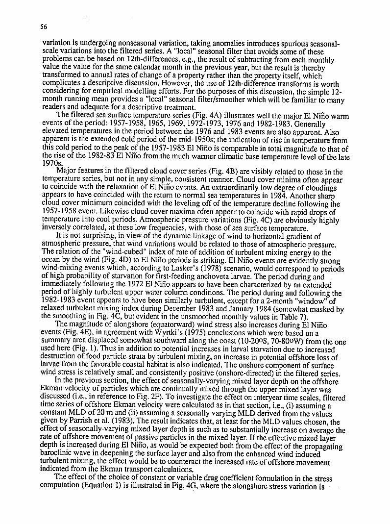
56
variation is undergoing nonseasonal variation taking anomalies introduces spurious seasonalshyscale variations into the filtered series A local seasonal filter that avoids some of these problems can be based on 12th-differences eg the result of subtracting from each monthlyvalue the value for the same calendar month in the previous year but the result is therebytransformed to annual rates of change of a property rather than the property itself which complicates a descriptive discussion However the use of 12th-difference transforms is worth considering for empirical modelling efforts For the purposes of this discussion the simple 12shymonth running mean provides a local seasonal filtersmoother which will be familiar to manyreaders and adequate for a descriptive treatment
The filtered sea surface temperature series (Fig 4A) illustrates well the major El Niio warm events of the period 1957-1958 1965 1969 1972-1973 1976 and 1982-1983 Generallyelevated temperatures in the period between the 1976 and 1983 events are also apparent Also apparent is the extended cold period of the mid- 1950s the indication of rise in temperature from this cold period to the peak of the 1957-1983 El Niiio is comparable in total magnitude to that of the rise of the 1982-83 El Ni-io from the much warmer climatic base temperature level of the late 1970s
Major features in the filtered cloud cover series (Fig 4B) are visibly related to those in the temperature series but not in any simple consistent manner Cloud cover minima often appearto coincide with the relaxation of El Nifio events An extraordinarily low degree of cloudings appears to have coincided with the return to normal sea temperatures in 1984 Another sharpcloud cover minimum coincided with the leveling off of the temperature decline following the 1957-1958 event Likewise cloud cover maxima often appear to coincide with rapid drops of temperature into cool periods Atmospheric pressure variations (Fig 4C) are obviously highlyinversely correlated at these low frequencies with those of sea surface temperature
It is not surprising in view of the dynamic linkage of wind to horizontal gradient of atmospheric pressure that wind variations would be related to those of atmospheric pressureThe relation of the wind-cubed index of rate of addition of turbulent mixing energy to the ocean by the wind (Fig 4D) to El Nifio periods is striking El Niffo events are evidently strongwind-mixing events which according to Laskers (1978) scenario would correspond to periodsof high probability of starvation for first-feeding anchoveta larvae The period during and immediately following the 1972 El Nifio appears to have been characterized by an extended period of highly turbulent upper water column conditions The period during and following the 1982-1983 event appears to have been similarly turbulent except for a 2-month window of relaxed turbulent mixing index during December 1983 and January 1984 (somewhat masked bythe smoothing in Fig 4C but evident in the unsmoothed monthly values in Table 7)
The magnitude of alongshore (equatorward) wind stress also increases during El Nifio events (Fig 4E) in agreement with Wyrtkis (1975) conclusions which were based on a summary area displaced somewhat southward along the coast (10-200S 70-80oW) from the oneused here (Fig 1) Thus in addition to potential increases in larval starvation due to increased destruction of food particle strata by turbulent mixing an increase in potential offshore loss of larvae from the favorable coastal habitat is also indicated The onshore component of surface wind stress is relatively small and consistently positive (onshore-directed) in the filtered series
In the previous section the effect of seasonally-varying mixed layer depth on the offshore Ekman velocity of particles which are continually mixed through the upper mixed layer was discussed (ie in reference to Fig 2F) To investigate the effect on interyear time scales filtered time series of offshore Ekman velocity were calculated as in that section ie (i) assuming a constant MLD of 20 m and (ii) assuming a seasonally varying MLD derived from the values given by Parrish et al (1983) The result indicates that at least for the MLD values chosen the effect of seasonally-varying mixed layer depth is such as to substantially increase on average the rate of offshore movement of passive particles in the mixed layer If the effective mixed layerdepth is increased during El Nifio as would be expected both from the effect of the propagatingbaroclinic wave in deepening the surface layer and also from the enhanced wind induced turbulent mixing the effect would be to counteract the increased rate of offshore movement indicated from the Ekman transport calculations
The effect of the choice of constant or variable drag coefficient formulation in the stress computation (Equation 1)is illustrated in Fig 4G where the alongshore stress variation is
25 S24- 28
V)
21
is-1_
55
20
is-__var
60 65
Year
70 75 80
85
020-
---
-1612
-- shy
55
60 65
Year
70
tp
constant coefficientviable coefficient
75 80
-
85
B H
1220 -
- -681 oW210
60
55
56
60 65 Yea
70 75
80
)
85
2 20
u ~190 55 60 65
Year 70
75
80 s
-
85
10135-
13
E10120shy
30
10125-a
010o 55 60 65
Year 70 75 80 85
22
Year
Fig 4 Low-frquency nonseasonal variations 12-month running means of monthly time series values (Note that the SI-standard heat flux units watts per square meter may be converted to calories per square centimeter per day by multiplying by the factor 2064)
-t-4
Ln
D
iso- 80constant 70
coefficientshyvariable coefficient
200
040
B-30 -20shy
55 60 65 Y aYear 80 85 55 60 65 Ya 70 75 80 85
E K
5
Eon~shor
C- 2
tol_
lonshore com ponent copnn --
ID
ISO
160
is 140
12D
I
I00
constant coefficient -
variable coefficient
-
55 60 65 70 75
YeauirY e a r
80 85
~ ~iii~
55 60 65 70
Year -Y 008
75 85
mnl mean lnaitude
2ee e pe ue c pe d by mliyn h factor52064)81b
- seasonally-varying MID ----- e 795 55
6 -
60 0
65 775 80 85 55 60 1 IIl5 I
65 7075 08 Y e ar YYore a -
Fig 4 Continued Low-frequency nonseasonal varitions 12-month running -neans of monthly time series values (Note that the Sl-standard heat flux units watts per square meter may be converted to calories per square centimeter perday by multiplying by the factor 2064)
59
plotted in terms of its directly proportional transform offshore Ekman transport The variable coefficient formulation produces generally lower estimates of stress due to the influence of the stability of the lower atmospheric boundary layer over upwelling-affected surface waters However the differences essentially disappear during the period of relaxation of the intense El Niios of 1957-1958 and 1982-1983 A possible explanation is the tendency for a less stable atmosphere in contact with the ocean surface due to residual warmth which would linger longerin the ocean than in the atmosphere due to the much greater heat storage capacity of water compared to that of air
The filtered series of estimates of absorption of solar radiation by the ocean (QS) exhibits some interesting patterns (Fig 4H) Since the variables that control the solar radiation estimate (Equation 2) derived from a maritime report at any given latitude are calendar date and cloud cover it is not surprising that maxima in Fig 4H often correspond to minima in Fig 4B and vice versa However there are discernible differences between the two series that result from the interaction of the cloud cover variations with the seasonal changes in solar height in the solar radiation time series An impressive feature in the solar radiation series is the early largeshyamplitude alternation consisting of deep minimum of solar radiation entering the ocean corresponding to the early part of the intense 1954-1955 cold period followed by a sharp highlyerratic rise to a high peak in early 1960 In addition the entire period of the 1960s and the first half of the 1970s appears to have been characterized by low absorption of solar radiation relative to the more recent period since 1976
The long-wave radiative heat loss (QB) tends to be an order of magnitude smaller than the short-wave absorption but varies very similarly (Fig 41) This similarity is perhaps explainablein the similar dependence of both types of estimate on cloud cover with the sea surface temperature dependence in the long-wave radiation estimate (Equation 3) being related seasonally to the solar height dependence in the solar radiation estimate (Equation 2) There mayalso be some actual causal effect of the long period variations in solar radiation on the sea temperature dependence in the long-wave radiation estimate
The filtered series of evaporative heat loss (QE) delineates the various El Niffo episodes and the 1954-1955 cold period in a very similar fashion to the sea surface temperature series (Fig4J) The long-term variation in vapor pressure difference between the sea surface and the overlying atmosphere (Equation 4) is apparently very closely linked to that of sea surface temperature As discussed above the wind speed dependence is also a strong function of these climate scale events The effect of choice of constant or variable transfer coefficient apparentlymakes very little difference except during the mid-1950s cold period where increased stability of the air over the cold ocean apparently inhibited the turbulent exchange of latent heat according to the variable coefficient formulation
The net ocean-atmosphere heat exchange series (QN) indicates long-term variations in net ocean heat gain such that minima are associated with El Nifio episodes and maxima with cold periods The variations appear to be controlled to a substantial extent by the evaporative heat loss (Fig 4J) This is so because the variations in heat gain by absorption of short-wave solar radiation (Fig4H) are partially offset by the highly correlated variations in long-wave radiative heat loss (Fig 41) The net effect of the choice of variable or constant transfer coefficient formulations in the evaporative and conductive components is a slight general lowering of the magnitude oi net heat gain in the variable coefficient case This difference is due primarily to the stability effect on the conductive heat loss term as discussed in the previous section in reference to Fig 2E where the average change in the mean net value of this component approximately 5 wattsm2 corresponds in general to the approximate difference between the curves in Fig 4K except in the mid-1950s where stability effects on the evaporative heat loss term are appreciable
In order to check for long-period variations in the distribution of observations within the summary area (Fig 1) filtered series of the monthly averages of the respective latitudinal and longitudinal locations of reports were prepared (Fig 4L) Since the coastline is oriented somewhat northwest to southeast variations in the two curves which tend tc parallel each other in the figure will tend to yield a resultant displacement in the alongshore direction More serious with respect to the long-term homogeneity of the monthly series herein presented are variations in Fig 4L where the curves are changing in the opposite sense ie where the net displacement of the mean position of reports is in the onshore-offshore direction these situations are
60
Table 1 Numbers of observations in monthly samples used to construct timeseries For each month the first number refers to observations used in constructing the values in Tables 2456 amp 7 (sea temperature atmosphericpressure wind stress components and wind cubed index the 2nd number refers to observations used in constructing the values in Table 4 (cloudcover) the 3rd number refers to observations used for values in Tables 8910 amp 11 (heat exchange components)
Jan Feb Mar Apr May Jun1953 21 19 191 29 29 291 22 22 191 23 23 101 33 33 331 16 16 61954 61 57 40 19 19 171 21 21 211 59 59 531 42 39 391 36 34 24 1955 24 22 201 35 35 291 16 15 121 9 9 51 24 24 13 35 35 301956 - 41 38 151 17 15 151 16 16 31 39 39 211 22 22 161 20 20 71957 32 32 321 25 24 151 98 98 471 38 38 291 25 25 211 53 52 33 1958 153 153 1061 74 73 441 69 69 341 84 84 281 67 66 441110 107 521959 128 125 511162 162 491143 138 371115 112 371 97 96 211 67 67 43 1960 98 95 421148 146 1101166 166 1051151 146 1011171 164 1351 85 82 591961 148 147 1271124 124 901115 111 941183 180 1501 89 86 661130 128 1041962 185 183 1271149 148 1341163 162 1421157 155 1221114 111 1051177 177 147 1963 78 76 711103 102 1021182 181 1671180 177 1701157 156 1491185 185 1851964 129 12S 981138 137 1351 82 81 811 76 76 761 45 45 451 52 52 521965 59 59 581 75 71 701137 137 1371 99 99 961139 136 1361139 139 1381966 107 107 1071 82 82 821113 112 1111106 106 1061117 113 1101137 137 137 1967 111 109 1021 60 52 521 80 80 781147 144 1441 75 74 741 66 66 661968 76 76 761128 127 1271108 108 1081139 137 1371 91 87 871111 109 1081969 67 67 67 87 84 841134 131 1311 91 91 911 56 56 561102 102 102 1970 90 87 821 57 57 531103 100 901 51 51 481 99 98 921208 206 200 1971 103 101 931 81 77 751 89 89 891 53 53 521 44 44 441 22 22 211972 109 108 1041 54 52 511 49 49 471 85 85 851 81 81 811 56 56 561973 55 54 401 44 44 391 89 89 891 50 50 481 58 58 561 57 54 471974 84 78 781 63 63 581113 109 1001 57 54 541119 118 1171 73 72 721975 59 57 561 73 72 691140 140 1401 99 92 901140 138 1361116 115 114 1976 70 69 681 20 19 191 76 73 711 59 59 551 71 71 701 49 44 401977 51 51 511109 106 1051 79 79 731101 99 941 93 88 871 70 70 69 1978 57 56 561 65 65 621 71 69 671 92 92 881 71 71 711 41 40 35 1979 97 96 89 58 57 511105 104 981 85 85 771 83 80 741 48 45 341980 96 93 801106 105 931125 123 1021 75 70 541151 146 1191246 201 98 1981 116 113 851 90 89 821139 137 1241108 103 951115 108 791128 124 1081982 91 89 821 90 90 801152 146 1391100 98 881103 98 801 54 54 41 1983 68 64 541126 126 1161 94 91 861 76 72 611 93 92 831 61 61 551984 90 75 261 99 80 391 90 59 141 75 41 161 58 39 61 56 49 29
Jul Aug Sep Oct Nov Dec 1953 10 10 91 39 35 261 29 28 251 18 18 11 24 24 181 19 18 111954 40 39 381 14 14 101 27 26 221 43 371 30 30 61 18 18 9 1955 17 17 121 37 36 211 35 35 61 45 44 341 27 27 201 13 13 51956 45 45 361 21 21 211 29 29 211 41 40 291 63 61 201 24 24 61957 27 27 111 24 24 211 64 64 381112 110 651100 99 531115 115 86 1958 51 51 271159 159 831 96 93 441113 108 471115 110 631 58 43 26 1959 100 100 571103 101 391 85 81 421 74 74 211110 110 551114 114 85 1960 169 168 1471114 111 671142 142 941 75 75 461 63 63 231 82 81 591961 108 107 821155 155 1421153 151 1411128 127 801197 197 1921135 133 118 1962 213 212 1931168 168 1591 81 81 751129 125 1251173 172 1521 91 88 791963 120 120 1201 70 70 701110 110 l011 70 70 701 61 61 581 56 56 53 1964 90 88 871 71 65 641 94 94 881129 127 1211 62 61 581105 104 1021965 92 92 921119 117 1151 99 99 981 67 67 671177 176 1761111 Ill 1061966 116 112 1121122 118 1181185 182 1821131 125 1251 89 89 881123 123 123 1967 89 87 871 67 67 671 84 84 841 76 71 711 73 73 731 99 97 971968 58 58 581 82 81 811 59 59 561111 109 1081118 118 1181 66 65 65 1969 70 70 701 86 84 841108 97 921102 102 971137 137 1271101 101 96 1970 75 74 741 66 65 651 91 90 901 50 50 501127 125 1241 68 68 671971 43 43 421 58 58 541 28 28 231 51 51 471 78 78 781 34 31 30 1972 35 32 301 60 58 541 32 32 291 81 74 741 31 28 261 51 51 48 1973 81 75 741105 92 881 89 84 821 55 54 501100 98 981 71 71 701974 102 101 1011 90 89 891 67 66 661 53 52 501 78 78 771 44 44 441975 67 66 651 53 48 471 70 68 681 70 65 601 68 68 671 88 88 88 1976 74 74 721 21 21 181 88 87 861 76 76 731 46 44 441 58 57 57 1977 55 54 531 55 51 511 73 70 681106 104 1041183 166 1631 67 59 31978 37 33 301 5T S1 501 73 72 671 53 49 491 99 79 761 87 87 851979 80 75 631137 108 q01116 109 821 84 77 531 77 75 591 39 35 26 1980 281 233 53j2tj7 182 9CI148 131 941129 118 891 80 74 611 70 66 471981 169 161 781174 159 631122 111 921127 115 971174 155 1421154 147 127 1982 78 74 681 78 70 661 71 62 551106 102 811132 124 1131 93 89 511983 124 121 841145 116 4F1 70 48 191156 150 901 73 73 241 96 90 321984 104 90 411113 87 81 75 --54 14195 51 69 251 62 40 77 61 35
61
Table 2 Sea surface temperature in degrees Celsius The standard error of the mean appears within parentheses to the right of the mean temperaturevalue
Jan Feb Mar Ap May Jun 1953 2114(50) 2308(64) 2463(51) 2478(49) 2279(37) 2052(46) 1954 1855(33) 2286(46) 2201(42) 1636(29) 1786(23) 1695(25) 1955 2172(39) 1850(52) 2101(85) 1901(37) 1789(85) 1667(30) 1956 1990(44) 1764(82) 2166(46) 2071(29) 1990(41) 1922(29) 1957 1947(47) 2483(48) 2526(21) 2453(37) 2476(48) 2315(27) 1958 2315(11) 2500(19) 2452(25) 2283(30) 2163(35) 2042(18) 1959 2045(21) 2308(18) 2449(15) 2154(25) 2090(18) 1926(25) 1960 2197(18) 2274(18) 2270(19) 2058(18) 1909(14) 1822(18) 1961 2230(15) 2324(20) 2161(21) 1994(15) 2024(21) 1867(15) 1962 2129(14) 2212(18) 2037(18) 1941(18) 1868(18) 1892(12) 1963 2072(24) 2267(17) 2215(16) 2021(17) 2101(13) 1898(10) 1964 2144(12) 2241(14) 2091(22) 2066(37) 1838(26) 1735(24) 1965 2175(26) 2309(27) 2396(15) 2454(21) 2408(20) 2211(14) 1966 2209(20) 2362(20) 2196(25) 2085(24) 1988(24) 1867(16) 1967 2002(22) 2212(22) 2186(23) 2061(19) 1911(24) 1813(30)
1968 1967(21) 2221(21) 2178(22) 1860(20) 1849(30) 1731(20) 1969 2228(23) 2236(23) 2425(18) 2351(23) 2294(25) 2092(22) 1970 2171(26) 2194(43) 2251(26) 2040(33) 1873(21) 1685(14) 1971 1970(19) 2034(29) 1970(25) 2163(36) 1980(32) 1846(46) 1972 2094(25) 2438(41) 2517(37) 2297(24) 23U5(22) 2168(24) 1973 2422(25) 2440(39) 2252(20) 1954(31) 1916(37) 1736(35) 1974 2072(30) 2200(36) 2210(31) 2135(36) 2136(24) 1951(19) 1975 2125(28) 2241(24) 2341(19) 2221(27) 2081(21) 1867(18) 1976 2116(30) 2338(64) 2296(33) 2245(35) 2164(28) 2123(30) 1977 2369(22) 2346(19) 2244(32) 2044(28) 1977(24) 1966(27) 1978 2106(24) 2346(25) 2257(25) 2269(32) 2007(34) 1995(49) 1979 2242(19) 2311(28) 2362(22) 2271(26) 2037(31) 2061(45) 1980 2169(25) 2322(21) 2421(21) 2248(29) 2181(17) 2084(13) 1981 2090(26) 2280(22) 2210(24) 2099(28) 2073(20) 1944(16) 1982 2133(22) 2262(30) 2165(23) 2120(24) 2101(22) 2115(41) 1983 2642(19) 2738(19) 2799(14) 2793(20) 2772(15) 2593(30) 1984 2213(221 2278(291 2192(261 2095(33) 1917(31) 1949f281
Jul Aug Sep Oct Nov Dec 1953 1978(27) 1906(21) 1820(34) 1824(35) 1872(40) 1881(41) 1954 1460(35) 1557(41) 1491(31) 1422(29) 1711(26) 1924(54) 1955 1768(53) 1554(45) 1571(28) 1469(37) 1709(24) 1812(37) 1956 1694(24) 1765(37) 1748(29) 1675(19) 1838(29) 1923(40) 1957 2243(34) 1928(34) 1894(19) 1923(17) 1907(16) 2075(16) 1958 1963(26) 1737(10) 1780(15) 1790(13) 1898(18) 2025(31) 1959 1755(15) 1680(12) 1664(18) 1777(20) 1904(20) 1935(15) 1960 1765(10) 1742(12) 1717(11) 1753(18) 1878(24) 2059(17) 1961 1004(22) 1762(11) 1687(11) 1736(16) 1854(14) 1939(17) 1962 1730(09) 1727(10) 1677(10) 1689(10) 1808(12) 1949(21) 1963 1870(13) 1824(17) 1800(11) 1755(16) 1854(28) 1972(17) 1964 1710(18) 1611(20) 1611(14) 1640(15) 1831(32) 1976(19) 1965 2059(20) 2000(20) 1779(16) 1826(23) 1876(13) 2149(15) 1966 1800(12) 1675(13) 1681(10) 1737(12) 1813(17) 1977(20) 1967 1740(16) 1646(17) 1S76(13) 1609(21) 1690(18) 1822(21) 1968 1764(23) 1705(17) 1826(38) 1765(17) 1767(16) 2082(24) 1969 1844(20) 1801(17) 1736(19) 1824(16) 1839(13) 1949(15) 1970 1572(12) 1619(13) 1633(28) 1636(25) 1794(16) 1829(21) 1971 2800(28) 1727(23) 1632(26) 1705(27) 1834(15) 1981(35) 1972 2118(36) 2177(23) 1929(36) 1917(35) 2061(32) 2173(31) 1973 1688(32) 1604(16) 1580(22) 1611(31) 1727(24) 1901(30) 1974 1812(15) 1748(15) 1670(31) 1691(32) 1896(23) 1983(35) 1975 1846(25) 1768(36) 1571(24) 1559(20) 1624(15) 1874(24) 1976 2118(20) 1951(55) 1900(23) 1919(25) 2004(23) 2146(15) 1977 1854(25) 1723(22) 1721(28) 1849(28) 1895(16) 1945(24) 1978 1849(35) 1691(33) 1727(25) 1811(25) 1940(30) 2049(24) 1979 1873(25) 1830(26) 1901(28) 1853(23) 1925(27) 2104(38) 1980 2004(11) 1835(13) 1777(15) 1839(23) 1895(27) 2021(21) 1961 1808(17) 1824(11) 1767(24) 1786(23) 1898(15) 2029(15) 1982 1965(18) 1834(23) 1900(36) 2061(22) 2303(17) 2519(21) 1983 2324(23) 2126(21) 1957(25) 1989(14) 2025(22) 2154(27) 1984 1952(231 1837(131 1844(18) 1827(281 1970(311 2020(311
62
Table 3 Total cloud amount Valvas indicate mean fraction of sky obscuredThe standard error of the mean appaars in parentheses to the right of each mean value
Jan Feb Mar ApM May1953 66(06) s8(06) 43(06) 43(08) 54(06)
Jun 76(10)1954 59(05) 75(05) 69(07) 35(04) 85(05) 74(07)1955 55(07) 61(06) 60(09) 06(04) 69(08) 90(04)1956 66(05) 46(l0) 40(06) 33(06) 65(08) 89(06)
1957 48(07) o(05) 56(03) 57(05) 5(06) 76(04)1958 60(03) 68(03) 63(03) 32(04) 54(04) 83(03)1959 40(03) 58(C2) 66(02) 60(03) 83(03) 78(04)1960 so(03) 30(03) 38(02) 44(03) 52(03) 63(05)1961 65(03) 44(03) 65(03) 50(03) 49(04) 79(03)1962 55(02) 54(03) 48(03) 56(03) 53(04) 79(03)1963 50(04) 52(03) 61(02) 52(03) 66(03) 81(02)1964 64(03) 66(03) 57(04) 51(04) 72(06) 63(06)1965 54(04) 49(04) 61(02) 60(03) 63(03) 64(03)1966 56(03) 44(03) 57(03) 45(03) 62(03) 76(03)1967 72(03) 51(05) 56(03) 51(03) 46(04) 82(04)1968 52(04) 52(03) 45(03) 38(03) 65(04) 75(03)1969 57(04) 55(04) 58(03) 57(04) 70(05) 81(03)1970 59(04) 43(04) 37(03) 43(05) 62(04) 81(02)1971 51(03) 3s(04) 48(03) 52(05) 68(06) 8s(06)1972 53(04) 49(04) 64(03) 53(04) 69(04) 78(04)1973 67(03) 61(05) 60(04) 49(04) 40(05) 70(05)1974 59(03) 52(04) 53(03) 53(05) 77(03) 8(02)1975 69(04) 50(04) 60(02) 54(03) 72(03) 86(03)1976 61(04) 59(08) 63(03) 55(05) 62(04) 87(04)1977 54(05) 68(03) 55(04) 34(03) 53(04) 71(04)1978 53(04) 65(04) 45(04) 57(04) 54(05) 68(07)1979 s0(03) 53(04) 56(03) 44(03) 67(04) 79(05)1980 57(03) 53(03) 58(03) 48(04) 57(03) 80(02)1981 66(03) 63(03) 51(03) 57(03) 66(03)1982 80(03)
60(03) 58(03) 55(03) 52(03) 58(04) 84(04)1983 52(04) 47(02) 63(03) 70(03) 75(03) 74(04)1984 42(041 43(031 45(03) 40(04) 34(051 74(041
Jul Aug SeD Oct NOV Dec1953 65(14) 91(04) 74(07) 74(07) 81(06) 67(07)1954 79(05) 86(07) 92(05) 89(04) 72(05) 75(08)1955 97(02) 90(04) 90(04) 80(05) 61(08) 44(10)1956 85(05) 82(08) 64(05) 62(05) 73(05) 49(08)1957 79(06) 72(08) 85(04) 72(03) 72(03) 64(03)1958 79(05) 80(03) 90(02) 81(03) 52(04) 45(06)1959 78(03) 78(03) 79(04) 79(03) 63(04) 51(03)1960 72(03) 81(03) 90(02) 89(03) 63(05) 67(04)1961 94(01) 83(02) 90(02) 78(03) 61(02) 60(03)1962 90(02) 93(02) 86(03) 88(02) 77(02) 46(04)1963 80(03) 80(04) 88(02) 82(04) 77(04) 68(05)1964 87(03) 87(03) 86(03) 88(02) 77(04) 51(03)1965 88(03) 90(02) 92(02) 86(03) 75(02) 61(03)1966 77(03) 83(03) 85(02) 89(02) 83(03) 61(03)1967 88(03) 91(03) 84(03) 85(04) 86(03) 47(04)1968 80(05) 93(02) 88(03) 83(03) 76(03)1969 86(04) 83103) 91(02) 82(03) 68(03) 50(04)
56(04) 1970 87(04) 91(03) 85(03) 95(02) 59(03) 64(04)1971 94(02) 88(03) 92(03) 853(05) 65(04) 65(06)1972 83(05) 80(04) 87(04) 78(04) 86(05) 67(05)1973 82(03) 91(02) 87(03) 80(04) 81(03) 72(04)1974 91(02) 89(03) 88(03) 75(05) 72(04) 57(05)1975 86(03) 89(03) 89(03) 77(04) 78(04) 64(04)1976 80(04) 93(03) 77(03) 81(03) 78(04) 53(04)1977 89(03) 86(04) 83(04) 81(03) 72(02) 41(05)1978 9s(0l) 84(04) 80(104) 8l(04) 68(04) 50(03)1979 865(03) 8l(03) 83(03) 8(03) 8o(03) 49(06)1980 90(01) 90(02) 81(02) 82(02) 69(04) 48(04)1981 87(02) 83(02) 92(02) 67(03) 63(03) 51(03)1982 80(04) 88(03) 82(03) 76(03) 75(03) 58(03)1983 72(03) 68(03) 66(06) 80(02) 58(04) 49(04)1984 81(031 75(031 86(031 91(03 70o051 52(041
63
Table 4 Atmospheric pressure at sea level Add 10000 to the mean valuesin the table to yield pressure in millibars The standard error of the mean appears in parentheses to the right of each mean value the standard errors are given (directly) in millibars
Jan Feb Mar A r May Jun1951J 112( 3) 104( 1) 111( 3) 132( 5) 125( 2) 145( 5)1954 123( 2) 122( 4) 102( 4) 213( 3) 135( 3) 147( 3)1955 125( 3) 109( 2) 104( 4) 119( 5) 136( 2) 152( 2)1956 115( 2) 107( 4) 111( 3) 109( 3) 120( 2) l0O( 6)1957 128( 2) 86( 3) 109( 3) 99( 3) 123( 2) 123( 2)1958 219( 2) 115( 2) 72( 4) 98( 3) 115( 2) 132( 1)1959 120( 2) 109( 1) 115( 2) 112( 1) 133( 2) 142( 2)1960 116( 2) 215( 2) 113( 2) 115( 1) 127( 1) 137( 2)1961 106( 4) 106( 2) 106( 2) 112( 4) 129( 1) 136( 2)1962 130( 1) 118( 2) 120( 1) 128( 2) 140( 2) 153( 1)1963 129( 2) 136( 2) 112( 1) 135( 4) 132( 1) 142( 1)1964 23( 1) 105( 1) 112( 2) 122( 2) 127( 4) 142( 2)1965 117( 1) 102( 2) 110( 2) 115( 1) 113( 2) 129( 2)1966 106( 2) 102( 2) 202( 1) 118( 2) 132( 1) 146( 1)1967 115( 2) 123( 2) 120( 2) 113( 2) 131( 2) 143( 2)1968 113( 2) 117( 1) 126( 2) 129( 1) 143( 2) 156( 1)1969 112( 3) 96( 1) 114( 2) 113( 1) 115( 2) 13s( 2)1970 128( 2) 110( 2) 118( 1) 117( 2) 145( 2) 144( 1)1971 119( 2) 108( 2) 108( 2) 123( 2) 138( 3) 153( o4)1972 109( 2) 210( 3) 103( 2) 115( 2) 118( 2) 121( 2)1973 105( 4) 118( 2) 107( 2) 115( 3) 130( 3) 145( 2)1974 119( 5) 118( 2) 125( 2) 126( 3) 137( 3) 142( 2)1975 115( 3) 119( 2) 114( 1) 119( 2) 135( 1) 140( 1)1976 121( 3) 116( 7) 106( 1) 119( 2) 125( 2) 120( 2)1977 204( 3) 212( 1) 100( 2) 120( 4) 126( 2) 137( 2)1978 139( 3) 101( 7) 120( 2) 123( 2) 128( 2) 150( 3)1979 122( 1) 119( 3) 114( 2) 110( 3) 133( 3) 155( 5)1980 129( 2) 123( 2) 93( 2) 105( 2) 129( 2) 145( 3)1981 139( 3) 108( 2) 114( 2) 121( 2) 143( 2) 18( 4)1982 126( 5) 114( 2) 104( 2) 121( 2) 126( 2) 129( 3)1983 91( 3) 97( 2) 91( 2) 95( 2) 96( 3) 116( 2)1984 125(21 107( 3) 107( 51 131f 3 137( 7) 139( 21 1953 137( 5) 134( 2) 130( 2) 150( 5) 140( 3) 132( 4)1954 138( 3) 143( 4) 138( 3) 148( 2) 145( 2) 130( 3)1955 157( 3) 151( 3) 154( 3) 161( 3) 140( 2) 131( 5)1956 149( 3) 137( 4) 144( 3) 141( 2) 142( 5) 94( 6)1957 130( 3) 140( 3) 125( 3) 134( 2) 128( 2) 122( 2)1958 141( 3) 139( 2) 140( 3) 127( 2) 128( 2) 106(l7)2959 136( 1) 141( 2) 131( 2) 137( 2) 133( 2) 122( 3)1960 145( 1) 145( 2) 141( 1) 140( 2) 111( 2 135( 3)1961 144( 2) 144( 1) 147( 1) 13b( 1) 147( 2) 132( 1)1962 144( 1) 152( 2) 139( 3) 153( 2) 106(14) 138( 2)1963 143( 2) 136( 3) 138( 4) 144( 1) 154( 4) 124( 2)1964 148( 1) 148( 2) 142( 2) 143( 2) 131( 2) 132( 1)1965 126( 2) 140( 2) 141( 2) 139( 2) 121( 2) 116( 1)1966 140( 1) 149( 1) 148( 1) 141( 2) 136( 2) 123( 1)1967 142( 2) 145( 2) 152( 2) 140( 2) 134( 2) 130( 2)1968 148( 2) 152( 1) 140( 3) 135( 2) 141( 1) 126( 2)1969 143( 2) 149( 2) 130( 1) 138( 1) 132( 2) 122( 1)2970 155( 1) 144( 2) 138( 2) 139( 3) 139( 1) 110( 2)2971 137( 3) 143( 7) 145( 4) 153( 2) 140( 1) 123( 3)1972 125( 6) 128( 3) 129( 3) 131( 2) 122( 3) 218( 6)1973 147( 4) 148( 2) 152( 3) 151( 2) 143( 2) 148( 2)1974 138( 4) 147( 2) 149( 2) 140( 2) 137( 1) 126( 2)1975 152( 2) 151( 3) 155( 2) 153( 2) 151( 2) 135( 2)1976 133( 2) 146( 6) 133( 4) 137( 3) 139( 2) 104( 2)1977 135( 3) 143( 2) 147( 2) 142( 2) 137( 2) 124( 2)1978 139( 4) 141( 2) 145( 2) 138( 2) 123( 2) 123( 2)1979 149( 2) 142( 3) 147( 3) 148( 2) 141( 3) 125( 9)1980 151( 2) 152( 2) 141( 4) 138( 3) 138( 2) 137( 5)1981 150( 3) 160( 2) 148( 2) 139( 2) 134( 2) 119( 1)1982 120( 2) 129( 2) 141( 3) 129( 2) 106( 2) 100( 2)1983 118( 2) 142( 4) 150( 5) 136( 2) 133( 7) 142( 4)1984 126( 4 153( 31 148( 51 145( 31 142( 11 118( 31
64
Table 5 Alongshore component (positive equatorward) of wind stress on the sea surface Units are dynes per square centimeter The standard error of the mean appears in parentheses to the right of the mean alongshore stress valueValues in this table multiplied by the factor 395 (see text) yield offshoreBkma transport in cubic meters per second across each meter width
Jan FeP Mar A P May Jun 1953 36(06) 32(05) 44(07) 99(20) 83(09) 37(10)1954 24(03) 41(14) 10(02) 46(05) 56(08) 46(08) 1955 40(09) 16(03) 53(18) 18(08) 63(11) 45(09)1956 16(02) 25(07) 67(10) 83(09) 85(13) 50(05)29S 31(06) 53(21) 76(05) 86(10) 57(06) 76(07) 1958 40(05) 42(05) 45(05) 61(06) 57(07) 46(04)1959 34(03) 28(02) 40(03) 42(04) 30(03) 59(07)1960 23(03) 27(02) 41(03) 49(04) 53(09) 45(04)1962 20(02) 27(03) 39(04) 48(03) 70(06) 48(05)1962 42(02) 34(03) 47(03) 52(04) 51(04) 60(04)1963 32(04) 39(03) 61(03) 47(03) 59(04) 33(03)1964 49(04) 44(03) 51(05) 71(07) 63(07) 58(12)1965 29(04) 40(05) 40(03) 53(06) 97(07) 58(04)1966 60(04) 61(06) 46(04) 75(06) 59(05) 62(04)2967 40(04) 36(04) 29(03) 30(03) 37(04) 71(10)1968 15(02) 40(05) 36(03) 36(03) 34(05) 65(05)1969 29(04) 26(04) 47(04) 56(04) 45(07) 89(08)1970 33(04) 16(05) 40(05) 56(06) 55(05) 52(04)2971 17(04) 36(04) 34(03) 59(08) 43(07) 73(23)1972 29(03) 34(04) 56(11) 55(04) 42(04) 67(08)1973 57(06) 38(05) 73(05) 60(08) 67(11) 51(07)1974 32(04) 42(05) 48(04) 68(07) 71(05) 66(07)1975 40(04) 35(04) 72(05) 63(05) 74(04) 63(06)1976 21(04) 17(04) l(05) 77(07) 72(07) 56(08)1977 32(06) 56(06) 38(04) 57(05) 47(05) 67(05)1978 37(05) 47(06) 62(07) 71(08) 59(07) 72(12)2979 49(05) 54(09) 54(04) 68(05) 69(07) 92(14)1980 44(04) 47(05) 49(04) 49(05) 89(07) 58(03)2981 52(04) 30(03) 46(04) 54(04) 53(05) 84(08)1982 35(04) 47(04) 63(04) 55(04) 65(06) 91(12)1983 69(06) 66(04) 46(05) 74(08) 75(06) 107(09) 1984 26(041 53(111 80(131 31(11) 83(181 07(131
Jul Aug See Oct No Dec 1953 70(22) 36(05) 46(06) 53(08) 62(08) 27(05)1954 52(07) 89(21) 83(09) 24(02) 30(04) 20(04)1955 46(09) 88(14) 66(10) 65(12) 60(08) l1(04)1956 69(09) 52(13) 64(05) 50(C8) 45(04) 45(08) 2957 101(11) 54(08) 75(07) 56(06) 44(04) 56(04)2958 51(05) 71(06) 49(04) 43(04) 26(03) 39(05)1959 38(04) 53(04) 48(07) 44(05) 31(03) 23(03)1960 59(05) 55(04) 51(04) 48(06) 34(03) 36(04)1961 67(06) 50(04) 50(04) 40(03) 38(02) 31(03)1962 60(04) 49(04) 60(06) 49(04) 51(04) 23(02)1963 54(05) 48(06) 72(05) 72(11) 53(06) 36(04)1964 62(05) 71(09) 73(08) 57(04) 36(05) 42(04)1965 63(05) 84(07) 87(07) 60(07) 49(03) 49(04)1966 76(04) 74(06) 59(03) 52(04) 26(03) 26(02)1967 54(05) 72(07) 74(09) 73(09) 46(05) 35(06)1968 90(10) 72(08) 64(08) 59(03) 51(03) 62(08)1969 53(06) 71(08) 59(05) 42(04) 28(03) 37(04)1970 1971
47(06) 52(05) 45(04) 50(07) 41(03) 27(05)40(08) 77(112) 64(12) 71(08) 43(05) 49(09) 1972 90(11) 81(10) 132(19) 49(05) 35(04) 72(15)1973 70(11) 116(12) 101(11) 71(09) 58(05) 37(06)2974 73(05) 64(08) 72(07) 67(07) 68(05) 45(06)1975 64(07) 91(10) 73(05) 51(05) 36(04) 35(05)1976 59(05) 69(16) 80(06) 67(06) 64(06) 52(06)1977 94(11) 83(10) 47(06) 46(04) 157(04) 55(o06) 1978 87(14) 69(08) 73(09) 54(06) 51(06) 47(05)1979 65(07) 66(09) 72(07) 65(05) 54(05) 46(07)1980 101(04) 74(04) 75(06) 65(05) 47(04) 49(06)1981 77(07) 64(04) 85(09) 41(04) 57(04) 42(03)1982 89(08) 63(06) 96(12) 84(06) 73(04) 66(05)2983 86(06) 69(06) 77(07) 60(05) 38(10) 23(05)1984 61(061 76(061 64(071 60(041 86f061 58(05)
Table 6 Onshore component of wind stress on the sea surface Units are dyres per square centimeter The standard error of the mean appears in parentheses to the right of each mean onsho7e stress value
1953 1954 1955
Jan 10(03) 04(0)
-04(03)
Fab 02(03) 07(05)02(01)
Mar 00(05) 00(01)19(07)
APr -12(04) 10(02)09(08)
May 02(04)
-04(03)-01(03)
Jun -06(05) 04(02)
-01(03)
1956 1957 1958 1959 1960 1961 1962
06(03)
05(02)
07(01)
05(01)
07(01)
03(01)
08(01)
48(03) -06(05) 08(02) 07(01) 04(01) 01(01) 01(02)
o8(08) -06(02) 09(02) 01(02) 05(ol) 06(02) 04(01)
01(04) -04(03) 01(02) 06(01) 04(02) 05(01) 02(02)
0(05)
00(04)
02(02)
04(02)
03(01)
03(02)
02(02)
10(04)
06(03)
08(02)
17(03)
02(02)
04(02) -03(01)
1963 1964 1965
06(01)
05(02)
06(02)
02(02)
03(01)
05(02)
08(01)
04(02)
01(01)
01(01) -07(03) 06(02)
0(02)
CL(04) -08(03)
01(01)
06(03)
03(02) 1966 1967 1968
05(02)
02(02)
03(01)
06(02)
08(02)
02(02)
09(03)
02(02)
04(01)
-06(02) 03(01) 02(01)
03(02)
09(02)
01(03)
06(02)
08(05)
01(02) 1969 1970 1971 1972 1973 1974 1975 1976 1977 1978 1979 1980
04(01)
04(02)
05(02)
04(01)
13(03)
04(02)
02(02)
03(01)
07(02)
04(03)
03(02)
08(02)
04(02) -08(05) 04(02)
-06(05) 07(02) 02(02) 07(02) 01(04)
-03(03) 09(03)
-08(04) 06(02)
00(01)
05(02)
00(02) -06(07) -02(02) -04(02) -05(02) 01(02) 06(02) 05(03) 08(03) 02(02)
03(02)
10(03)
03(04)
03(02)
13(04)
02(04) -04(02) -06(04) 07(03)
-03(02) 03(02) 03(03)
05(03)
08(02) -03(02) 00(02)
-02(04) -01(02) 00(02) 01(02) 02(02) 03(02)
-03(03) -05(03)
-03(03) 03(01)
-08(07) 06(04) 15(05) 03(03)
-01(02) 03(04)
-01(03) -07(05) -04(04) -08(02)
1981 1982 1983 1984
02(02)
06(02)
15(03)
06(02) Jul
00(02)
1O(03)
00(02) -04(021
Aug
05(02)
00(02) -03(03) -08(061
Sep
-01(02) -O1(02) -01(07) -10(061
Oct
01(02)
06(03)
07(03)
08(07) NOv
01(03) -09(06) 05(04) 14(051
Dec 1953 1954
15(04)
06(03) 06(02)
-02(ll) 12(03) 19(08)
07(07)
04(01) 08(03) 21(05)
04(02)
08(02) 1955 1956 1957 1958 1959 1960 1961 1962
o8(04)
02(06) -05(09) 12(03) 04(02) 06(02) 04(02) 05(01)
04(06)
31(08)
18(05)
23(05)
12(02)
07(02)
03(01)
12(02)
09(04)
13(04)
05(03)
12(02)
17(06)
06(02)
08(02)
10(02)
09(02)
14(03)
07(02)
20(03)
05(01)
67(02)
15(03)
08(02)
12(05)
06(03)
10(02)
05(01)
05(01)
02(01)
03(01)
08(01)
o5(ol)
06(02)
11(02)
06(02)
04(01)
06(02)
04(01)
09(02) 1963 03(02) 01(02) 09(02) 05(03) 03(04) 07(02) 1964 1965 1966 1967 1968 1969 1970 1971
04(02)
01(03)
05(02)
tB(02)
3(04)
02(02)
07(02)
01(03)
05(05) -02(02) 15(03) 06(04) 09(03)
-02(02) 08(02) 14(04)
10(03)
10(03)
08(02) -01(03) 12(05) 08(02) 10(02)
-01(03)
11(02)
17(04)
15(02)
09(03)
11(02)
04(01)
18(04)
00(03)
05(02)
13(03)
06(01)
03(02)
08(01)
07(01)
12(03)
06(02)
04(02)
08(02)
02(01)
12(03) -06(04) 09(02) 09(03)
-02(04) 1972 1973
04(04) -03(04)
07(03)
01(05) 12(08) 01(06)
10(03)
01(05) 19(04) 01(02)
14(03)
06(03) 1974 1975
02(02)
06(03) 04(03) 03(05)
13(03)
06(03) 12(03) 11(03)
03(03)
os(03) 13(03) 04(02)
1976 1977 1978 1979
03(04)
05(07) -11(05) -01(03)
-01(06) -10(04) 04(04) 10(03)
09(03)
10(03)
07(03) -02(04)
15(03)
08(02)
08(03)
07(02)
02(04)
07(01)
07(02)
oo(03)
13(04)
02(03)
05(02)
06(06) 1980 1981 1982 19831984
-12(02) -04(03) 05(04) -03(02)07(051
-02(03) -05(01) 04(02)
-o(03) -22051
04(03)
01(03)
01(06) -10(03)03(04)
05(02)
07(02)
15(04)
02(03)02(041
06(02)
05(02)
09(02)
04(03)-09(031
-01(02) -04(01) 08(02) 04(03)-01(031
66
Table 7 Wind cubed index of rate of addition to the water column bywind of turbulent mixing energy the
The standard errors of the mean appear inparentheses to the right of each mean index value 3 3 Nominal units are m sec
Jan Feb Mar Aot may Jun1953 130( 34) 107( 19) 162( 35) 473(140) 354( 44) 130( 47)1954 75( 16) 205( 85) 19( 4) 186( 32) 210( 46) 174( 41)1955 132( 40) 37( 9) 316(101) 93( 22) 238( 67) 177( 50)1956 58( 15) 91( 30) 287( 46) 355( 51) 377( 68) 182( 25)1957 201( 22) 220( 44) 310( 23) 375( 64) 201( 27) 337( 42)2958 184( 48) 171( 32) 181( 25) 260( 37) 244( 46) 192( 21)1959 116( 13) 94( 8) 143( 14) 154( 18) 104( 16) 300( 47)1960 84( 11) 86( 10) 151( 15) 207( 18) 307( 95) 161( 19)1961 71( 9) 83( 11) 173( 24) 17C( 13) 301( 37) 204( 26)2962 156( 12) 127( 16) 171( 14) 220( 24) 197( 20) 226( 19)1963 113( 19) 141( 19) 252( 17) 176( a) 230( 20) 113( 13)1964 188( 20) 156( 14) 198( 27) 295( 36) 248( 41) 315(117)1965 100( 17 155( 33) 144( 16) 238( 51) 467( 45) 232( 20)1966 247( 26) 263( 30) 213( 25) 312( 35) 252( 34) 263( 24)1967 147( 16) 143( 25) 94( 13) 102( 11) 140( 20) 387( 80)1968 47( 10) 172( 3G) 126( 15) 120( 11) 142( 25) 272( 25)1969 97( 16) 113( 19) 174( 18) 206( 23) 193( 34) 432( 68)1970 121( 17) 148( 36) 166( 3R) 232( 35) 227( 25) 218( 20)1971 92( 16) 128( 25) 120( 15) 266( 42)1972 102( 14) 146( 33) 346( 70)
135( 30) 404(162)214( 25) 146( 18) 315( 51)2973 247( 29) 136( 21) 292( 26) 333( 49) 314( 75) 279( 52)1974 121( 17) 155( 24) 181( 20) 308( 62) 300( 29) 295( 39)1975 135( 18) 140( 22) 308( 24) 251( 21) 304( 24) 272( 33)1976 76( 22) 68( 19) 196( 27) 326( 39) 308( 36) 248( 53)1977 134( 44) 251( 40) 158( 21) 265( 27) 191( 27) 263( 30)1978 150( 22) 214( 33) 280( 44) 316( 54) 246( 35) 327( 91)1979 202( 33) 250( 54) 241( 23) 282( 29) 331( 38) 459(122)1980 179( 19) 212( 32) 203( 21) 194( 23) 441( 47) 241( 18)1981 205( 22) 104( 13) 195( 19) 212( 21) 226( 27) 431( 73)1982 134( 21) 199( 20) 259( 19) 201( 20) 300( 29) 491( 97)1983 319( 31)1984 110( 211 262( 18) 203( 21) 420(117) 373( 35) 539( 61)307(120) 534M17 288f110) 636(1591 522(1161
Jul Aug San Oct Nov Dec1953 332(129) 125( 26) 179( 34) 217( 43) 243( 50) 74( 16)1954 207( 37) 445(135) 439( 73) 64( 8) 161( 33) 59( 13)1955 179( 41) 460(100) 308( 76) 322( 79) 266( 42) 30( 13)1956 324( 56) 346( 65) 261( 29) 237( 56) 184( 23) 158( 35)1957 484( 66) 253( 52) 331( 45) 261( 38) 189( 24) 238( 22)1958 214( 25) 474( 56) 214( 26) 228( 30) 92( 16) 152( 26)2959 138( 16) 233( 23) 303( 76) 164( 23) 108( 15) 82( 13)1960 260( 32) 222( 25) 201( 19) 198( 35) 99( 12) 144( 24)2961 290( 39) 191( 17) 211( 20) 199( 24) 136( 12) 100( 12)1962 265( 22) 236( 23) 267( 32) 199( 20) 212( 19) 96( 15)1963 220( 26) 176( 25) 320( 31) 376( 72) 222( 33) 131( 19)1964 250( 25) 385( 89) 372( 58) 242( 22) 132( 20) 164( 21)1965 263( 29) 392( 45) 442( 52) 319( 44) 240( 21) 193( 20)1966 317( 29) 388( 39) 245( 18) 243( 28) 95( 12) 83( 10)1967 222( 28) 336( 41) 357( 59) 369( 57) 180( 30) 280( 45)2968 442( 61) 352( 56) 326( 62) 243( 19) 192( 16) 283( 42)1969 237( 33) 312( 52) 272( 29) 154( 26) 104( 13) 151( 23)1970 248( 34) 212( 28) 186( 22) 251( 50) 194( 24) 139( 22)1971 190( 49) 425( 71) 258( 66) 302( 49) 169( 23) 199( 57)1972 423( 63) 400( 67) 805(139) 220( 27) 156( 25) 407(157)1973 S69( 81) 784( 81) 675( 74) 348( 66) 237( 28) 179( 37)197v 299( 28) 317( 57) 352( 45) 295( 42) 274( 28Y 195( 31)1975 284( 35) 461( 58) 316( 31) 235( 35) 143( 24) 147( 23)1976 264( 36) 377( 87) 370( 33) 328( 37) 270( 49) 235( 43)2977 529( 95) 392( 59) 229( 37) 189( 21) 241( 17) 220( 34)1978 434( 85) 310( 54) 350( 82) 226- 29) 237( 49) 203( 28)1979 290( 51) 433( 73) 350( 51) 274( 33) 233( 28) 226( 50)1980 458( 27) 354( 31) 382( 35) 271( 28) 181( 22) 188( 30)1981 420( 49) 244( 21) 457( 60) 166( 10) 249( 22) 146( 13)1982 438( 52) 270( 40) 549( 82) 454( 57) 316( 22) 275( 30)1983 379( 34) 330( 39) 318( 43) 277( 33) 227(111) 122( 32)1984 334i 58) 415( 881 328( 461 242( 30) 350( 27) 229( 221
67
Table 8 Daily total (both direct and diffuse) solar radiation absorbed bythe ocean Qs The standard error of the mean appears in parentheses to theright of each sean yalue Units are wattsM 2 (Values may be converted tounits of cal c ay by multiplying by the factor 2064)
Jan Feb Mar Aor May239(12) 253( 9) 262(11) 258(15)
Jun1953 193( 9) 182(22)1954 240( 9) 214(10) 227(12) 241( 6) 141( 7) 158(11)1955 250(12) 254(12) 236(17) 282( 8) 182(17) 125( 5)1956 255(16) 269(16) 257(31) 230(12) 181(14) 121( 3)1957 264(12) 203(11) 243( 7) 221( 8) 190(10) 153( 7)1958 244( 5) 236( 8) 243( 9) 248( 9) 202( 8) 148( 6)1959 287( 7) 247( 8) 241( 9) 208(10) 169(12) 144( 6)1960 268( 9) 269( 4) 283( 3) 236( 4) 204( 4) 167( 7)1961 242( 5) 276( 5) 228( 5) 221( 4) 205( 6) 140( 4)1962 258( 5) 257( 4) 260( 4) 214( 4) 192( 6) 143( 3)1963 263( 6) 265( 5) 240( 4) 217( 0) 176( 4) 139( 3)1964 243( 6) 236( 4) 242( 6) 223( 6) 162( 8) 161( 7)1965 257( 8) 268( 7) 236( 4) 218( 4) 183( 4) 165( 4)1966 252( 5) 279( 5) 246( 5) 236( 4) 182( 5) 148( 4)1967 218( 5) 264( 8) 244( 5) 230( 4) 207( 6) 138( 5)2968 250( 7) 263( 5) 265( 5) 244( 4) 174( 6) 149( 4)1969 248( 7) 257( 6) 238( 4) 216( 5) 168( 7) 140( 4)1970 245( 7) 274( 7) 280( 4) 236( 7) 178( 5) 140( 2)1971 264( 6) 255( 6) 261( 5) 230( 7) 169( 8) 130( 6)1972 256( 6) 271( 7) 237( 6) 221( 5) 170( 6) 145( 6)2973 236( 7) 247( 9) 237( 5) 229( 7) 216( 7) 151( 7)1974 250( 6) 268( 7) 257( 5) 219( 8) 156( 4) 131( 3)1975 234( 7) 268( 6) 240( 4) 224( 5) 163( 4) 131( 3)1976 245( 7) 248(13) 234( 5) 218( 8) 178( 6) 130( 5)1977 259( 8) 235( 4) 244( 6) 253( 4) 187( 5) 154( 5)1978 258( 8) 240( 7) 265( 6) 217( 6) 190( 6) 153( 9)1979 270( 5) 264( 7) 246( 5) 238( 5) 171( 5) 142( 7)1980 248( 6) 261( 5) 244( 5) 231( 7) 187( 4) 156( 5)1981 233( 5) 241( 5) 249( 5) 218( 5) 183( 6) 142( 3)1982 246( 6) 257( 5) 246( 4) 230( 5) 187( 5) 139( 6)1983 260( 8) 273( 4) 236( 5) 201( 5) 163( 4) 149( 5)2984 263( 91 268( 7) 260(101 223(10) 204(29) 142( 61Jul AUg SeD Oct Nov Dec1953 170(20) 142( 3) 204(12) 227(16) 211(13) 266(15)1954 149( 8) 144( 5) 158( 5) 192( 7) 225(19) 184(11)1955 123( 2) 154( 7) 159( 2) 217(10) 241(15) 263(26)1956 134( 7) 157(11) 184( 9) 198(10) 195( 9) 261(31)2957 143(11) 170(12) 186( 8) 211( 6) 216( 8) 235( 6)1958 154(11) 165( 5) 173( 7) 218( 9) 254( 8) 278(13)1959 154( 6) 169( 8) 190( 8) 218(13) 226( 7) 256( 6)1960 163( 4) 171( 6) 171( 4) 185( 5) 219(11) 235( 7)2961 126( 2) 159( 3) 170( 2) 210( 6) 243( 4) 240( 5)1962 133( 2) 148( 2) 173( 5) 193( 4) 211( 4) 258( 6)1963 145( 4) 167( 6) 177( 4) 204( 6) 212( 6) 229( 9)1964 138( 4) 154( 5) 183( 5) 191( 3) 210( 7) 257( 6)2965 135( 4) 148( 3) 169( 3) 197( 5) 219( 4) 241( 5)1966 151( 4) 162( 4) IPA( 3) 191( 3) 202( 4) 241( 5)2967 137( 4) 148( 3) 184( 5) 195( 5) 11v6( 5) 258( 6)1968 145( 5) 145( 3) 180( 5) 201( 4) 21( 5) 256( 7)1969 137( 5) 158( 4) 165( 3) 205( 5) 226( 5) 246( 6)2970 134( 4) 152( 4) 181( 4) 180( 3) 244( 5) 235( 7)1971 127( 2) 151( 4) 171( 7) 193( 7) 236( 6) 233(10)1972 138( 7) 161( 6) 183( 8) 209( 6) 195( 7) 229( 9)1973 142( 4) 149( 3) 174( 5) 205( 7) 208( 5) 221( 6)1974 127( 2) 154( 4) 175( 4) 27L8( 8) 222( 6) 250( 8)1975 134( 4) 156( 5) 173( 4) 212( 7) 211( 7) 234( 6)1976 147( 5) 143( 6) 194( 6) 206( 6) 212( 8) 257( 8)1977 134( 4) 155( 5) 187( 6) 204( 5) 223( 4) 270( 8)1978 126( 2) 160( 5) 187( 6) 205( 7) 231( 7) 264( 6)1979 138( 4) 167( 5) 179( 5) 217( 8) 210( 6) 252(12)1980 139( 5) 158( 4) 196( 5) 208( 5) 231( 8) 266( 9)1981 139( 4) 168( 6) 169( 2) 215( 6) 241( 4) 255( 4)1982 150( 6) 151( 4) 185( 6) 215( 5) 218( 5) 253( 6)1983 156( 5) 161( 7) 184(12) 198( 4) 258(12) 246(10)1984 157( 71 165( 61 175(161 185( 61 246(16) 242( 91
68
Table 9 Radiative heat lose Qs The standard error of the mean appears inparentheses to the right of each meap value Units are vattsm2 (Values maybe converted to units or cal cmi day by multiplying by the factor 2064)
Jan Feb Mar Apr May Jun1953 23( 2) 28( 2) 32( 3) 41( 5) 33( 3) 33(10)1954 26( 2) 16( 2) 22( 3) 43( 2) 16( 3) 30( 5)1955 30( 3) 27( 3) 29( 5) 60( 5) 29( 7) 1o( 2)1956 33( 5) 34( 5) 38(13) 41( 5) 28( 5) 7( 1)1957 33( 3) 13( 2) 26( 2) 29( 2) 28( 3) 21( 2)1958 24( 1) 22( 2) 27( 2) 39( 3) 36( 2) 20( 2)1959 43( 2) 24( 2) 28( 2) 29( 3) 22( 4) 28( 2)2960 32( 2) 33( 1) 44( 1) 37( 1) 38( 1) 31( 3)1961 26( 1) 34( 1) 25( 1) 34( 1) 39( 2) 19( 1)1962 31( 1) 31( 1) 36( 1) 30( 1) 35( 2) 21( 1)1963 33( 1) 31( 1) 27( 1) 34( 0) 27( 1) 18( 1)1964 27( 1) 23( 1) 30( 1) 34( 2) 23( 3) 30( 3)1965 33( 2) 34( 2) 27( 1) 27( 1) 27( 1) 28( 1)2966 30( 1) 37( 1) 29( 1) 38( 1) 29( 1) 21( 1)1967 20( 1) 33( 2) 30( 1) 34( 1) 38( 2) 19( 2)1968 33( 2) 33( 1) 36( 1) 44( 1) 28( 2) 23( 2)1969 29( 2) 30( 1) 28( 1) 29( 1) 23( 2) Is( 1)1970 29( 2) 35( 2) 42( 1) 37( 2) 29( 2) 19( 1)1972 34( 1) 30( 1) 35( 1) 34( 2) 26( 3) 15( 2)1972 32( 1) 32( 2) 24( 1) 31( 2) 24( 2) 18( 2)1973 22( 1) 24( 2) 27( 1) 36( 2) 43( 2) 25( 3)1974 30( 1) 33(2) 33( 1) 34( 2) 20( 1) 14( 1)1975 23( 1) 32(1) 27( 1) 32( 1) 23( 1) 15( 1)1976 27( 1) 30( 5) 25( 1) 31( 2) 29( 2) 14( 2)1977 30( 2) 22( 1) 29( 1) 43( 1) 33( 2) 25( 2)1978 31( 2) 24( 2) 34( 1) 31( 2) 33( 2) 25( 4)1979 33( 1) 30( 1) 27( 1) 36( 1) 25( 2) 20( 3)1980 30( 1) 29( 1) 28( 1) 34( 2) 31( 1) 25(2981 24( 1) 24( 1) 31( 1) 31( 1) 28( 2) l8(
2) 1)
1982 29( 1) 28( 1) 0( 1) 35( 1) 32( 2) 16( 2)1983 28( 2) 31( 1) 22( 1) 20( 1) Is( 1) 19( 2)1984 29(2 31( 21 32( 3) 29( 3) 37(10) 17(21
Jul Aug Sep Oct Noy Doc 1953 30( 9) 9( 1) 22( 4) 26( 5) 20( 4) 34( 3)2954 20( 3) 11( 3) 10( 2) 14( 2) 23( 5) 12( 3)1955 8( 0) 24( 3) 8( 1) 22( 3) 31( 5) 39(10)1956 16( 3) 28( 5) 15( 3) 19( 4) 25( 3) 35( 9)2957 17( 5) 19( 4) 18( 2) 21( 2) 22( 2) 25( 1)1958 22( 4) 20( 2) 14( 2) 25( 3) 35( 2) 43( 4)1959 22( 2) 19( 3) 21( 3) 24( 5) 25( 2) 34( 1)1960 27( 1) 23( 2) 15( 1) It( 1) 23( 3) 27( 2)1961 10( 0) 17( 1) 13( 0) 20( 2) 31( 1) 29( 1)1962 14( 0) 13( 0) 15( 1) 25( 1) 20( 1) 37( 2)1963 19( 1) 19( 2) 14( 1) 18( 2) 21( 2) 26( 2)1964 15( 1) 15( 2) 16( 1) 15( 1) 20( 2) 35( 1)1965 14( 1) 13( 1) 12( 0) 15( 1) 22( 1) 29( 1)1966 22( 1) Is( 1) 16( 1) 14( 1) 17( 1) 29( 1)1967 15( 1) 13( 1) 17( 2) 16( 2) 15( 1) 39( 2)1968 20(3) 11( 1) 14(1) 17(1) 22(1) 34(2)1969 15( 2) 17( 1) 12( 1) Is( 1) 26( 1) 31( 1)1970 15( 2) 13( 1) 16( 1) 10( 1) 32( 1) 29( 2)1971 ll( 1) 13( 1) 12( 2) 17( 3) 28( 2) 26( 3)1972 25( 2) 19( 2) 1s( 2) 20( 2) 15( 2) 25( 2)1973 17( 1) 12( 1) 15( 1) 20( 2) Is( 1) 23( 1)1974 13( 1) 14( 1) 15( 1) 23( 2) 23( 2) 32( 2)2975 15( 1) 14( 2) 14( 1) 23( 2) 20( 2) 28( 2)1976 19( 2) 11( 1) 20( 1) e(O1) 49( 2) 33( 2)2977 14( 1) 16( 2) 17( 2) 19( 1) 23( 1) 41( 2)1978 9( 0) 17( 2) 19( 2) 19( 2) 25( 2) 34( 1)1979 16( 2) 19( 2) 15( 1) 22( 2) 19( 2) 32( 4)1980 13( 1) 15( 1) 20( 1) 19( 1) 27( 2) 38( 2)1981 15( 1) 19( 2) 11( 0) 29( 2) 30( 1) 35( 1)1982 19( 2) 13( 1) 17( 2) 21( 1) 20( 1) 30( 1)1983 24( 2) 27( 2) 15( 3) 25( 1) 33( 3) 28( 3)1984 21( 21 12( 21 Is(81 11e 11 29( 51 29( 31
Table 10 Evaporative heat loss Qc The standard error of the mean appearsin parentheses to the right of each mean value Units are wattsma (Values may be converted to units of cal cmfdayby multiplying by the factor 2064)
Jan FEb Mar Apr May Jun 1953 3( 6) 34(10) 39( 8) 62(16) 97(11) 8( 9) 1954 -23( 5) 15( 4) 8( 3) -24( 4) 27( 5) 33( 4) 1955 22( 7) -26( 5) 39(16) 14(10) -14(12) 6( 5) 1956 17( 6) -27(13) -1(25) 39(11) 23( 9) 33( 6) 1957 -11( 3) 43( 9) 46(10) 68(13) 59( 8) 64(11) 1958 22(4) 65( 7) 31( 8) 37( 6) 49(11) 40( 5) 1959 15( 3) 15( 4) 59( 9) 42( 7) 21(10) 35( 6) 1960 11( 2) 18( 2) 32( 4) 22( 3) 15( 1) 24( 4) 1961 9( 2) 22( 2) 15( 4) 18( 2) 34( 4) 36( 4) 1962 22( 2) 33( 3) 16( 3) 16( 4) 26( 3) 50( 3) 1963 16( 3) 24( 2) 35( 3) 31( 0) 46( 3) 31( 2) 1964 25( 3) 25( 2) 19( 3) 34( 7) 28( 5) 30( 6) 1965 34( 6) 46( 5) 45( 3) 57( 5) 109( 7) 62( 3) 1966 36( 4) 63( 6) 30( 4) 51( 6) 44( 4) 40( 3) 1967 17( 2) 33( 4) 22( 3) 14( 2) 15( 3) 52( 8) 1968 6( 1) 36( 4) 24( 3) 12( 2) 26( 4) 38( 4) 1969 28( 4) 19( 3) 44( 3) 51( 5) 57( 6) 69( 5) 1970 29( 4) 31(11) 34( 4) 22( 6) 22( 4) 24( 2) 1971 14( 2) 11( 4) 6( 4) 40( 6) 39( 6) 46(10) 1972 20( 3) 48( 8) 62( 9) 48( 4) 62( 6) 31( 6) 1973 47(12) 28( 7) 39( 4) 30( 6) 28( 8) 32( 9) 1974 26( 3) 26( 5) 40( 4) 58( 9) 70( 5) 42( 4) 1975 26( 5) 21( 3) 55( 4) 54( 6) 70( 4) 44( 4) 1976 10( 2) 48(22) 32( 6) 62( 9) 64( 6) 57( 6) 1977 25( 4) 43( 5) 15( 4) 13( 5) 21( 4) 39( 6) 1978 21( 3) 38( 4) 34( 6) 54( 6) 23( 3) 62(11) 1979 27( 4) 35( 6) 30( 4) 38( 6) 45( 5) 40( 6) 1980 28( 6) 24( 5) 37( 4) 15( 3) 57( 5) 31( 4) 1981 12( 5) 19( 3) 14( 3) 29( 5) 42( 5) 51( 4) 1982 18( 2) 21( 5) 39( 5) 28( 3) 46( 5) 87(23) 1983 71( 5) 97( 5) 87( 4) 110(10) 124( 5) 125(14) 1984 4(101
Jul 31(71AqqSe
49(151 41(151Oct
-11(15)Noy
32( 8)Dec
1953 41(13) 53( 4) 29( 6) 33( 8) 32( 7) 8( 8) 1954 6( 6) 38(10) 17( 6) -8( 4) 15( 8) 25(12) 1955 46(10) 2(11) 8( 5) -9( 8) 9( 4) 2( 5) 1956 1957
69(11) 111(19)
35(10) 39(11)
49( 7) 54( 7)
21( 4) 42( 3)
69( 8) 35( 4)
-9( 3) 1( 6)
1958 56( 6) 35( 3) 31( 4) 40( 5) 21( 4) 27( 5) 1959 26( 2) 12( 3) 30( 7) 24(11) 13( 1) 2( 1) 1960 38( 3) 28( 3) 28( 2) 23( 4) 27( 5) 20( 5) 1961 34( 5) 37( 2) 28( 2) 18( 2) 27( 2) 14( 2) 1962 33( 2) 27( 2) 26( 3) 24( 2) 28( 2) 15( 2) 1963 40( 3) 38( 4) 43( 3) 37( 4) 36( 4) 24( 3) 1964 1965
40( 4) 60( 4)
37( 4) 64( 5)
31( 3) 36( 3)
30( 3) 29( 4)
17( 3) 36( 2)
27( 3) 33( 3)
1966 53( 3) 29( 2) 32( 2) 26( 2) 19( 2) 13( 1) 1967 36( 2) 34( 4) 22( 2) 19( 4) 24( 3) 26( 3) 1968 63( 6) 29( 3) 34( 3) 29( 2) 22( 2) 33( 6) 1969 41( 4) 43( 4) 31( 4) 16( 3) lo( 1) 15( 3) 1970 19( 3) 23( 3) 21( 3) 15( 3) 19( 2) 15( 3) 1971 39( 4) 44( 6) 31( 7) 34( 5) 19( 3) 31( 5) 1972 66(10) 105(10) 70(12) 40( 4) 37( 5) 42( 8) 1973 42( 7) 27( 6) 29( 4) 31( 5) 15( 5) 15( 4) 1974 61( 3) 32( 3) 25( 5) 28( 5) 37( 4) 33( 7) 1975 54( 6) 54( 6) 23( 5) 18( 3) 4( 2) 16( 3) 1976 74( 5) 30(17) 50( 4) 45( 7) 38( 6) 34( 3) 1977 48( 6) 32( 4) 19( 3) 48( 7) 23( 2) 18( 2) 1978 36(12) 30( 9) 32( 3) 31( 5) 25( 6) 24( 4) 1979 39( 4) 26( 3) 37( 3) 27( 4) 37( 7) 20( 5) 1980 28( 4) 29( 4) 28( 3) 34( 6) 20( 4) 15( 4) 1981 41( 6) 29( 3) 27( 4) 21( 3) 21( 3) 19( 2) 1982 71( 9) 30( 6) 34(10) 59( 4) 66( 5) 68(10) 1983 1984
91( 8) 4 8)
18(15) 37( 5)
46(17) s4(201
40( 4) 19C 8)
42( 7) 13(17)
15(10) 26( 81
70
Table 11 Net atmosphere - ocean heat exchange QN The standard error ofthe mean appears in parentheses to the right of each mean value Units arewattsM2 (Values may be converted to units of cal cii2 day by multiplyingby the factor 2064)
Jan Feb MaM Ar May Jun1953 220(13) 193(13) 196(13) 152(24) 51(16) 142(10)1954 261(11) 187(10) 200( 9) 247( 9) 101( 8) 89(10)1955 194(13) 273(11) 164(22) 211(16) 192(20) 115( 8)1956 208(12) 286(25) 232(22) 150(15) 137(18) 79( 9)1957 258(11) 143(16) 176(16) 125(17) 103(11) 63(16)1958 203( 7) 146( 9) 189(15) 171(10) 110(16) 81( 8)1959 236( 7) 215( 9) 155(13) 139(13) 125(18) 92( 9)1960 228( 8) 220( 4) 209( 6) 182( 5) 153( 4) 113( 7)1961 211( 5) 221( 4) 193( 7) 175( 4) 133( 7) 83( 6)1962 210( 5) 195( 5) 216( 6) 177( 6) 135( 6) 69( 4)1963 219( 7) 213( 5) 185( 5) 156( 0) 100( 6) 88( 3)1964 196( 6) 192( 4) 199( 6) 156(10) 111(11) 104(10)1965 190( 8) 187( 8) 164( 4) 135( 7) 35( 9) 69( 6)1966 188( 7) 179( 7) 187( 6) 145( 9) 108( 6) 86( 5)15L7 183( 5) 202( 6) 196( 4) 187( 4) 157( 5) 62( 9)1968 214( 5) 196( 5) 207( 4) 196( 4) 118( 6) 86( 5)1969 195( 6) 209( 6) 164( 5) 134( 7) 82(10) 41( 8)1970 185( 8) 212(13) 203( 7) 184(10) 130( 7) 101( 3)1971 220( 5) 219( 8) 230( 7) 155( 9) 99( 9) 67(13)1972 205( 5) 188(12) 150(11) 142( 7) 77(10) 99(10)1973 173(16) 203(11) 172( 7) 171(11) 153(11) 95(13)1974 197( 6) 211( 8) 187( 6) 128(13) 63( 7) 75( 5)1975 187( 8) 217( 6) 157( 7) 138( 9) 62( 7) 66( 6)1976 215( 6) 166(22) 179( 9) 124(14) 78( 9) 58( 8)1977 209( 9) 174( 6) 210( 9) 218( 9) 142( 7) 92( 9)1978 209( 8) 185( 7) 200( 9) 130(10) 139( 7) 64(15)1979 213( 8) 204( 9) 192( 7) 166(10) 101( 8) 82( 9)1980 198( 9) 217( 8) 184( 6) 190( 8) 99( 8) 103( 6)1981 211( 8) 202( 6) 214( 5) 166( 9) 114( 7) 75( 5)1982 207( 5) 220( 9) 182( 6) 172( 5) 111( 7) 26(31)1983 161( 8) 139( 7) 121( 7) 66(14) 8( 6) -8(17)1984 240(14) 213(111 180(17) 158(19) 197(24) 101(14)Jul Aua SOec Oct- Nov1953 Dec91(26) 74( 6) 151(11) 171(16) 257(14) 227(19)1954 135(14) 93(15) 138( 9) 201( 8) 183(19) 143(16)1955 58(14) 152(18) 140( 9) 222(15) 215(13) 226(17)1956 34(15) 97(15) 109( 8) 166( 9) 98(13) 245(22)1957 12(23) 110(18) 108(12) 144( 6)
1958 158( 7) 200( 9)69(12) 112( 6) 127( 8) 149( 9) 198( 8) 204(11)1959 104( 5) 139( 6) 140(11) 174(18) 189( 5) 224( 5)1960 95( 5) 120( 6) 129( 4) 252( 7) 172(12) 193( 7)1961 80(7) 103(4) 130(3) 173(5) 189(4) 203(5)1962 89( 3) 111( 3) 140( 6) 157( 4) 167( 4) 211( 5)1963 83( 5) 106( 7) 120( 6) 155( 7) 155( 7) 183( 811964 78( 6) 102( 7) 138( 5) 145( 4) 173( 6) 198( 5)1965 58( 7) 66( 7) 121( 5) 154( 6) 161( 4) 180( 5)1966 70( 5) 114( 4) 131( 3) 151( 3) 166( 4)1967 200( 4)85( 4) 97( 5) 144( 5) 169( 7) 156( 5) 196( 6)1968 55( 9) 108( 4) 135( 5) 157( 5) 174( 4) 192( 7)1969 75( 6) 93( 6) 121( 6) 170( 5) 192( 4) 203( 5)1970 102( 4) 117( 5) 146( 5) 165( 5) 195( 5) 198( 7)1971 71( 6) 92(10) 128(11) 142( 8) 194( 6) 176( 9)1972 51(15) 23(13) 98(17) 145( 7) 147( 8) 171(10)1973 77(11) 120(10) 144( 7) 157( 9) 187( 9) 191( 7)1974 46( 5) 106( 6) 141( 7) 175( 9) 166( 8) 183(12)1975 63( 8) 79(10) 144( 8) 178( 5) 197( 5) 195( 6)1976 52( 8) 116(25) 122( 8) 148( 9) 162( 9) 195( 7)1977 72( 9) 111( 6) 156( 7) 131(10) 181( 4) 222( 7)1978 89(16) 118(14) 138( 6) 158( 8) 191(10) 208( 7)1979 86( 7) 133( 6) 131( 6) 171( 7) 158(10) 207(10)1980 10S( 8) 117( 7) 154( 6) 156(10) 192( 9) 220( 9)1981 83( 8) 119( 6) 139( 5) 191( 6) 196( 5) 207( 4)1982 59(12) 114( 8) 144(14) 132( 6) 129( 7) 155(13)1983 34(10) 139(19) 136(25) 145( 7) 184(15) 216(15)1984 78(12) 108(101 121(36) 166(141 228(25) 190(11)
71
uncommon in the figure with the notable exception of the early 1970s and again in the early1980s The main point is that features in Fig 4L seem unrelated to any -majorfeatures apparentin the other series plotted in Fig 4 Thus the major effect of uneven distribution of reportsappears to be in increasing sampling variance rather than in introducing long-termnonhomogeneity in the various time series
Discussion
Since the 12-month running mean filter used to highlight the long-term variations in Fig 4incorporates no data more than 6 months previous or following the indicated multiyear features are certainly real and in no way represent artifacts of filtering and smoothing proceduresMoreover the interyear variations of annual mean values tend to be of similar magnitude to thecyclic seasonal components (Figs 2 and 3) making the separation of these scales in analysis ofeffects (eg on the biota) a difficult problem For example the impact of long-term variabilitywill generally depend on phase relationships with the seasonal variation Additional complications involve the adaptations of the biota not only the long-term evolutionaryadaptations of life cycle processes to regular cyclic effects but also lagged responses ofcommunity composition etc to events of the recent past (see Mendelsohn and Mendo this vol)
This area of the worlds ocean may be uniquely troublesome in these respects Because thePacific Ocean is so large it is much less subject to continental effects which amplifyseasonalities due to the low heat storage capacities of continents relative to oceans The apparentconsequence is much less forcing of Pacific Ocean processes to follow a regular seasonal cyclethan may be the case for example in the Atlantic the result is the dominance of interyearvariation in the Pacific (Picaut 1985) The location so near to the eastern terminus of theequatorial wave guide results in a focusing of variability initiated in various portions of the greatPacific ocean-atmosphere coupled system to particularly impact the ocean habitat off Peru Indeed this may constitute part of the explanation for the enormous biomasses of pelagic fishesthat have inhabited the region ie because of the intense irregular environmental variability asingle rather unspecialized fish species with very rapid population responses may be able todominate the system relatively free from predation and competition from more specialized lessresponsive species that would be more subject to the inefficiencies of multiple food-chain steps
We have noted that the interyear variations tend to involve groups of years In fact singlefeatures eg the 1982-1983 El Nigo the 1954-1955 cold period etc so dominate the series thatthe entire series length becomes a dominant scale of variability The result is that any sort ofassumption of stationarity must be somewhat unrealistic the real degrees of freedom useful forempirical analysis nearly vanish with respect to such features It is also apparent from evencasual inspection of Fig 4 that the index series presented in this paper are all highly interrelated in terms of major interyear features further exacerbating the problems of empirically sorting thevarious effects Any available mechanistic constraints provided by established physical orbiological principles that can be imposed on empirical analysis would of course be very helpfulin this situation
Variable vs Constant Transfer CoefficientFormulations
Some differences in the results of variable and constant transfer coefficient formulations inthe wind stress estimates (Equation 1) and in the estimates of certain of the heat exchangecomponents (Equations 4 5 and 6) have been noted in the discussions of both seasonal andinteryear variability The differences have mainly been in magnitude of the particular index withtemporal aspects of the variability appearing to be relatively unaffected An exception was theconductive component of heat exchange QCwhere the effect of stability in the atmosphericboundary layer introduced major discrepancies between the alternate formulations (Fig 3E)Fortunately QC is by far the smallest heat exchange component Some summary informationconcerning gross effects of the differences in the various series with respect to time series properties is indicated in Fig 5
72
- Raw series
S12 th - differences
- 12-month running means
coefficient of determination slope of regression
10 10 shy09 09 08 - n08 07 - 07 06 - 06 shy05 05 shy04 - 04
03 - 03 02 - 02 01 E I01 I0 Ii --
00 00 A Ty x OE QC ON ICy Xx QE QC QN
Fig 5Graphs of r2 (= coefficient of determination ie proportion of variation in one series explained by other series) and slope of the regression of the variable transfer coefficient formulation versus the constant transfer coshyefficient formulation of alongshore stress (7x) onshore stress (7ry) evaporative heat loss (QE) conductive heat loss (Q C) and net atmosphere-ocean heat exchange (QN)
In the case of alongshore component of wind stress the raw monthly series computed according to the two types of drag coefficient formulation are well correlated each accounting for more than 95 of the variance in the other When l2th-differencing was employed to remove the cyclic seasonal variations the correlation dropped only slightly this lower than expected drop in r2 must be due to a strong seasonality in the differences resulting from the two formulations Note that both the raw and l2th-differenced series pairs were much more highly correlated than the pair of 12-month running mean filtered series (which can be viewed in terms of directly proportional offshore Ekman transport in Fig 4G) The slope of the regression of the variable coefficient alongshore stress series on the constant coefficient series is nearly one to one in the raw series it drops to below 09 in the 12-differenced series but is above 095 in the filtered series
Slightly lower degrees of relationship are seen for the onshore component which tends to be much the smaller of the two stress components The respective formulations of evaporative heat loss (QE) were very highly correlated in raw and l2th-differenced series The degree of relationship fell only slightly after the 12-month running mean was applied In the case of the conductive heat loss term (QC) the two formulations gave substantially greater differences particularly after l2th-differencing or filtering In the case of net heat exchange (QN) the differences between the results of the two formulations appear not to be appreciable Note that in all cases the raw and 12-differenced series were more highly correlated between the constant and variable coefficient formulations than were the corresponding 12-month running mean filtered versions of the respective series thus the degree of relationship is even higher in the case of the unsmoothed series even after the seasonality is removed than can be seen in the comparative examples of filtered series in Fig 4
In view of the time series similarities the constant transfer coefficient versions of the respective index series are the only ones presented herein in tabular form (Tables 5 6 10 and 11) In view of the larger relative effect of the uncertainties as to proper formulation of the transfer coefficient for conductive heat loss and because its very small magnitude makes it relatively unimportant in any case no tabular series of QC is included Of course it would be possible to assemble the constant coefficient version of the QC series from the values in Tables 8 to 11
73
Offshore Ekman Velocity of the Mixed Layer
In discussing the inference of Parrish et al (1983) that the offshore Ekman transport should ideally be divided by the effective mixed layer depth to yield the net rate of offshore transport of drifting larvae which are passively mixed through the layer Bakun (1985) stressed theimportance of the qualification ideally Ekman transport is estimated from relatively abundant surface wind reports which reflect the fairly large spatial scales of atmospheric variation Mixed layer depth may vary on much shorter oceanic length scalesand must be determined from generally much less abundant subsurface observations In cases where the estimate of effectivemixed layer depth may be very imprecise the derived estimate of offshore Ekman velocity of the mixed layer could constitute a less reliable indicator of variability in this process than the Ekman transport alone
On long time scales mixed layer depth and wind stress observations are likely to be substantially correlated However within any given month it is probably not too bad an assumption to regard observations used to estimate these quantities (surface wind and subsurface temperature structure) as largely independent samples of the respective monthly distibutionsparticularly since there will normally be many more surface than subsurface reports In this casecombining the standard errors according to the rules for a quotient of independently observed quantities (eg Beers 1953) should provide a reasonable gauge of precision Thus the ratio of the standard error to the monthly mean derived net offshore Ekman velocity of the mixed layermight be reasonably estimated as being equivalent to the square root of the sum of the squares of the respective ratio of the standard errors to the monthly mean values of the Ekman transport and mixed layer depth components of the calculation
References
Anon 1966 Climatic change WMO Tech Note No 79 [WMO-No 195 TP 100] World Meteorological Organization Genes a 79 p
Bakun A 1985 Comparative studies and the recruitment problem searching for generalizations CaICOFI Rep 26 30-40 Bakun A 1986 Definition of environmental variability affecting biological processes in large marine ecosystems p 89-108 In
K Sherman and L Alexander (eds) Variability and management of large marine ecosystems American Association for the Advancement of Science Washington DC
Bakun A and RH Parrish 1980 Environmental inputs to fishery population models for cistem boundary current regions p 67shy104 In GD Sharp (ed) Workshop on the Effects of Environmental Variation on the Survival of Larval Pelagic Fishes Lima Peru April-May 1980 Workshop Report No 28 Intergovernmental Oceanographic Commission Unesco Paris
Bakun A and RH Parrish 1982 Turbulence transport and pelagic fish in the California and Peru Current systems CaCOFI Rep 23 99-112
Bakun A DR McLain and FV Mayo 1974 The mean annual cycle of upwelling off western North America as observed from surface measurements US Fish Bull 72 843-844
Beers Y 1953 Introduction to the theory of error Addison-Wesley Cambridge Massachusetts 65 p Brunt D 1932 Notes on radiation in the atmosphere I QJR Meteorol Soc 58 389-420 Budyko MI 1956 The heat balance of the earths surface (Teplovoi balans zenmoi poverkhnosti) Gidrometeorologicheskoe
izsatelstvo Leningrad 255 p (Transl 1958 259 p Off Tech Serv US Department of Commerce Washington DC PB 131692)
Deardorff JW 1968 Dependence of air-sea transfer coefficients on bulk stability J Geophys Res 73 2549-2557 Ekman VW 1905 On the influence of the earths rotation on ocean currents Ark Mat Astron Fys 2(11) 1-55 Elsberry RL and RW Garwood Jr 1978 Sea-surface temperature anomaly generation in relation to atmospheric storms Bull
Amer Meteorol Soc 59 786-789 Husby DH and CS Nelson 1982 Turbulence and vertical stability in the California Current CalCOFI Rep 23 113-129 Kraus EB 1972 Atmosphere-ocean interaction Oxford University Press London 229 pLarge WG and S Pond 1981 Open ocean momentum flux measurements in moderate to strong winds J Phys Oceanogr 11
324-336 Large WG and S Pond 1982 Sensible and latent heat flux measurements over the ocean 3Phys Oceanogr 12 464482
74
Lasker R 1978 The relation between oceanographic conditions and larval anchovy food in the California Current identification of factors leading to recruitment failure Rapp P-V R~un Cons int Explor Mer 173 212-230
List RJ 1949 Smithsonian Meteorological Tables 6th ed Smithson Misc Collec 114 Smithsonian Institution Press Washington DC 527 p
McLain DR RE Brainard and J G Norton 1985 Anomalous warm events in eastern boundary current systems CalCOFI Rep 26 51-64
Miyake Y 1952 A table of the saturated vapor pressure of sea water Oceanogr Mag 4 95-108 Murray FW 1967 On the computation of saturation vapor pressure JAppl lAeteorol 6 203-204 Nelson CS 1977 Wind stress and wind stress curl over the California Current US Department of Commerce NOAA Tech
Rep NMFS SSRF-71487 p Nelson CS and DM Husby 1983 Climatology of surface heat fluxes over the California Current region US Department of
Commerce NOAA Tech Rep NMFS SSRF-763 155 p Parrish RH A Bakun DM Husby and CS Nelson 1983 Comparative climatology of selected environmental pro-esses in
relation to eastern boundary pelagic fish reproduction p 731-777 In GD Sharp and J Csirke (eds) Proceedings of the Expert Consultation to Examine Changes in Abundance and Species Composition ofNeritic Fish Resources San Jose Costa Rica April 1983 FAO Fish Rep 291 (3) 731-777
Payne RE 1972 Albedo of the sea surface I Atmos Sci 29 959-970 Picaut J 1985 Major dynamics affecting the eastern tropical Atlantic and Pacific Oceans CalCOFI Rep 2641-50 Quinn WH DO Zopf KS Short and RTW Kuo Yang 1978 Historical trends and statistics of the Southern Oscillation El
Niuio and Indonesian droughts US Fish Bull 76 663-678 Reed RK 1976 On estimation of net long-wave radiation from the oceans J Geophys Res 81 5793-5794 Reed RK 1977 On estimating isolation over the ocean J Phys Oceanogr 7 482-485 Santander H 1980 Fluctuaciones del desove de anchoveta y algunos factores relacionados p 255-274a In GD Sharp (ed)
Workshop on the Effects of Environmental Variation on the Survival of Larval Pelagic Fishes Lima Peru April-May 1980 Workshop Report No 28 Intergovernmental Oceanographic Commission Unesco Paris
Seckel GR and FH Beaudry 1973 The radiation from sun and sky ov r the North Pacific Ocean (Abstr 033) EOS Trans Amer Geophys Un 541114
Siegel B 1983 El Nifio the world turns topsy-turvy The Los Angeles Times Aug 7 1983 p 1 18 19 Wyrtki K 1975 El Nifio - the dynamic response of the equatorial Pacific Ocean to atmospheric forcing J Phys Oceanogr 5
572-584
The Peruvian Anchoveta and Its Upwelling Ecosystem
Three Decades of Change
Edited by
D Pauly and ITsukayama
1987
INSTITUTO DEL MAR DEL PERU (IMARPE) CALLAO PERU
DEUTSCHE GESELLSCHAFT FUR TEPHNISCHE ZUSAMMENARBEIT (GTZ)GmbH ESCHBORN FEDERAL REPUBLIC OF GERMANY
INTERNATIONAL CENTER FOR LIVING AQUATIC RESOURCES MANAGEMENT MANILA PHILIPPINES
lii
1987
The Peruvian Anchoveta and its Upwelling EcosystemThree Decades of Change
EDrrh By
D PA LY I TsU AY~WA
Publisbd by Instituto del Mar del Peru (IMARPE) PO Box 22 Callao PeruDeutsche Gesellichaft for Technische Zusarrmmenarbeit (GTZ) GmbH Postfach 5180D-6236 Eschbom I bei FrankfurtMain Federal Republic ofGermany andInternational Center for Living Aquatic Rescurces Management (ICLARM)MC PO 1501 Makati Metro Manila Philippines
Printed in Manila Philippines
Pauly D and L Tsukayama Editors 1987 The Peruvian anchoveta and its upwelling ecosystem three decades of chunge ICLARMStudies and Reviews 15 351 p Instituto del Mar del Peru (IMARPE) Callao Peru Deutsche GesellIschaft fdr TechnLscheZusammenarbeit (G72) GmbH Eschbom Federal Republic of Germany and International Center for Uving AquaticResources Management Manila Philippines
ISSN 0115-4389 ISBN 971-1022346
Cover Time series of turbulence (above) and sea surface temperature (below) combined with pre-hispanic representation of Peruvianfisherman adapted from IMARPE report entitled Research on the Anchovy Models and Reality (1975)Artwork by Ovidio F Espiritu Jr
PROCOPA Contribution No 46
IClA Contribution N 391
iv
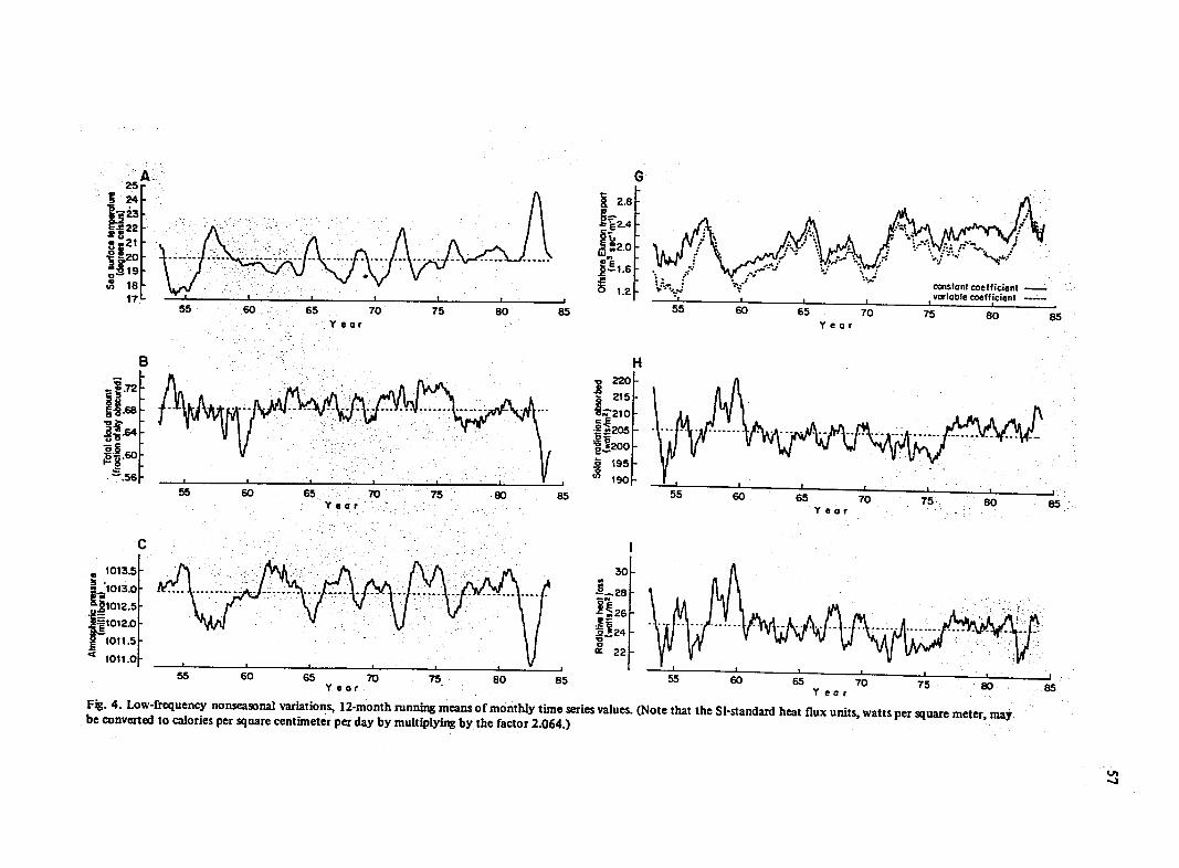
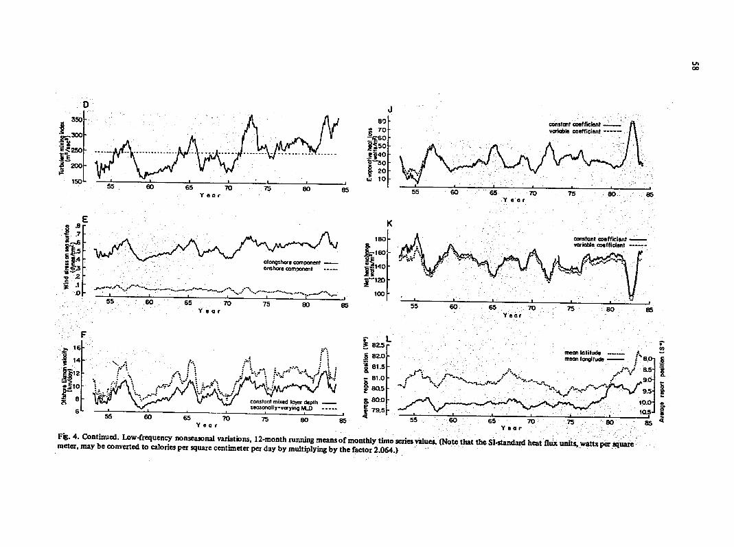
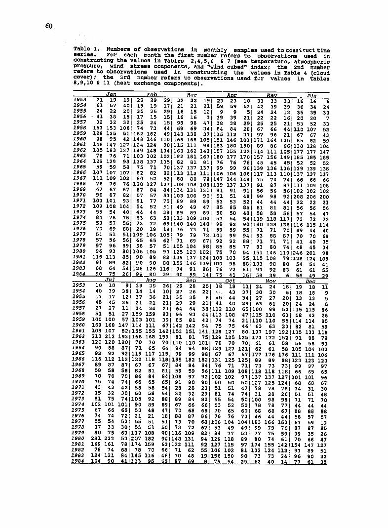
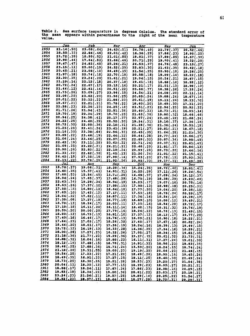
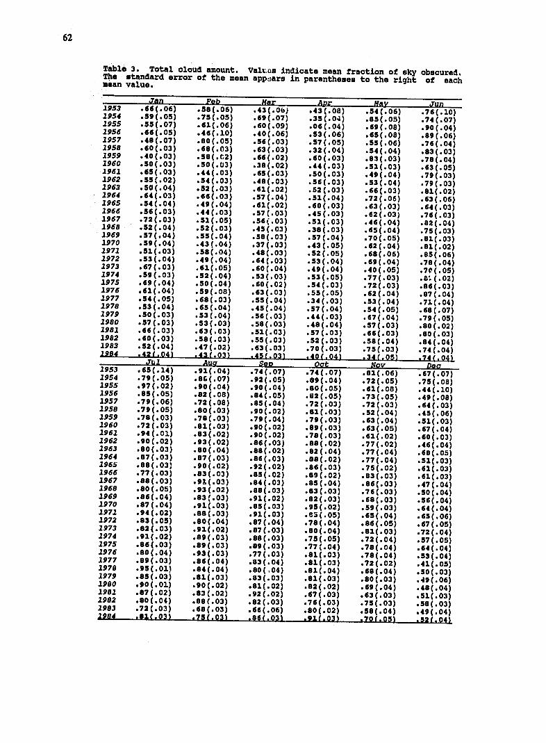
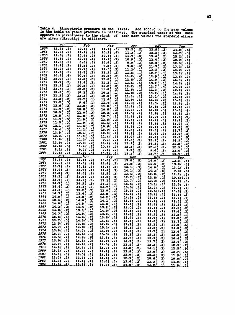
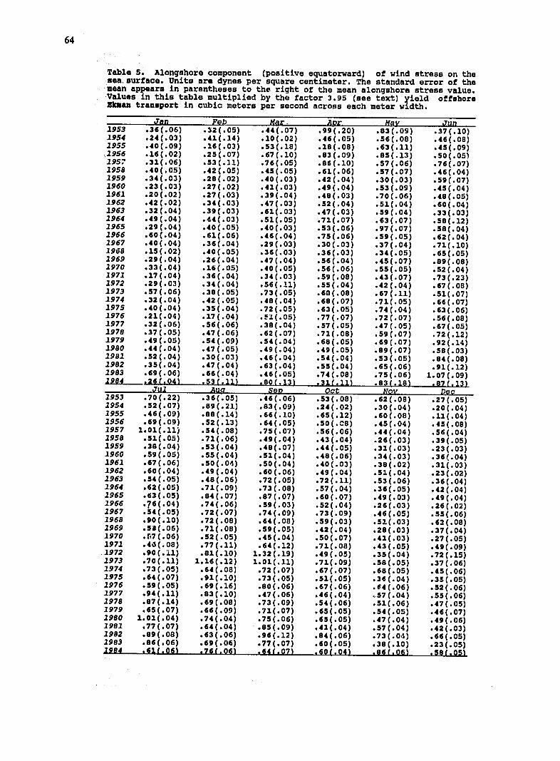
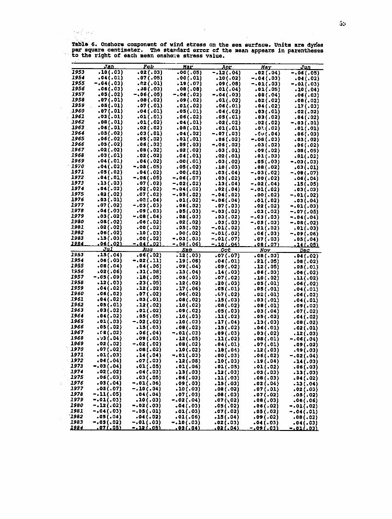
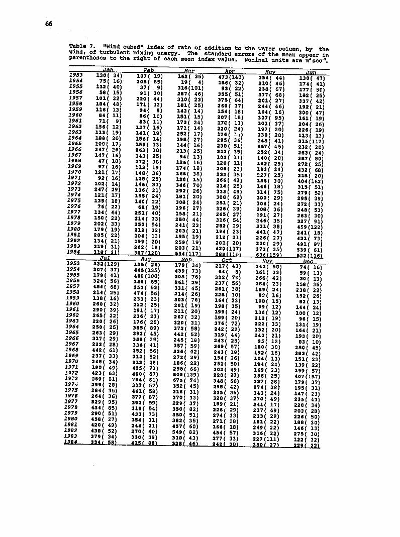
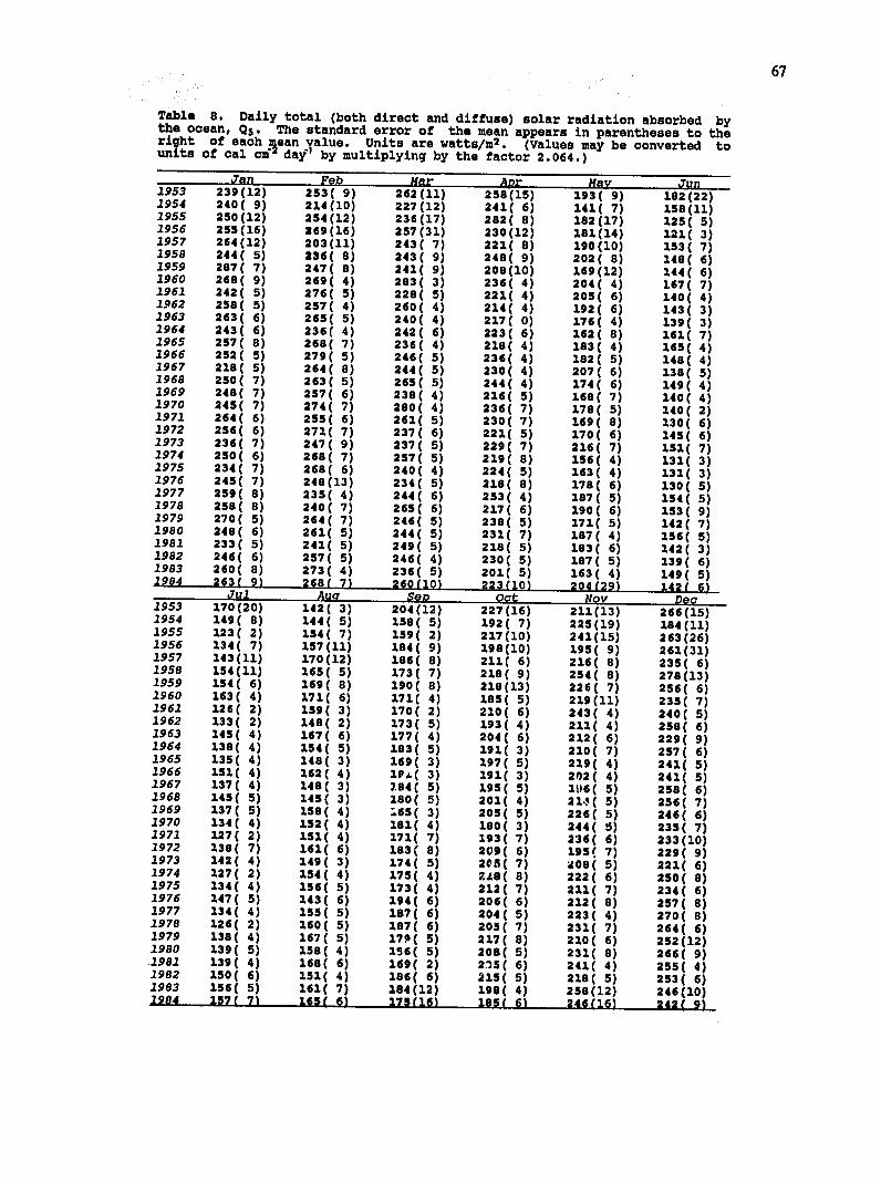
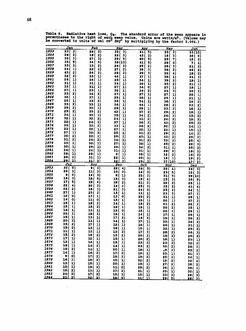
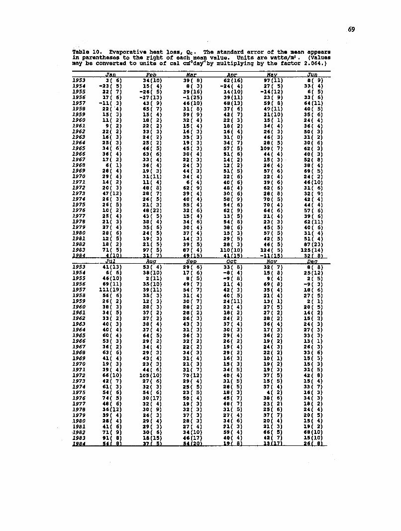
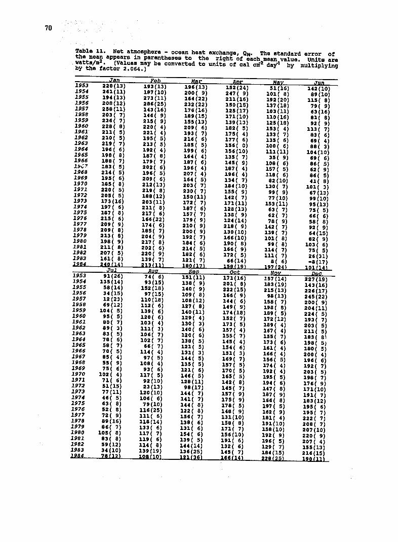
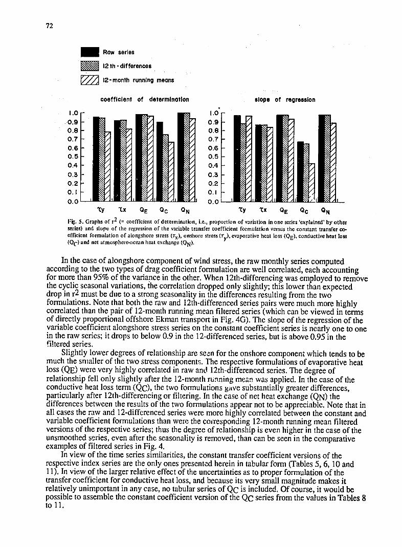
Related Documents