✬ ✫ ✩ ✪ Survival Analysis 27 P. Heagerty, VA/UW Summer 2005

Welcome message from author
This document is posted to help you gain knowledge. Please leave a comment to let me know what you think about it! Share it to your friends and learn new things together.
Transcript
'
&
$
%
Survival Analysis
27 P. Heagerty, VA/UW Summer 2005
'
&
$
%
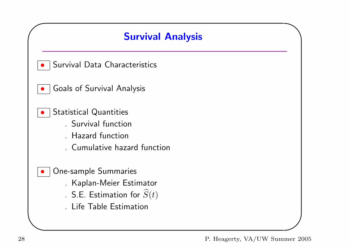
Survival Analysis
• Survival Data Characteristics
• Goals of Survival Analysis
• Statistical Quantities
. Survival function
. Hazard function
. Cumulative hazard function
• One-sample Summaries
. Kaplan-Meier Estimator
. S.E. Estimation for S(t)
. Life Table Estimation
28 P. Heagerty, VA/UW Summer 2005
'
&
$
%
• Two-sample Summaries
. Mantel-Haenszel / Log-rank Test
. Other tests – what? why?
• Regression Methods – Cox Regression
. Proportional hazards
. Interpretation of coefficients
. Estimation & Testing
. Survival function estimation
29 P. Heagerty, VA/UW Summer 2005
'
&
$
%
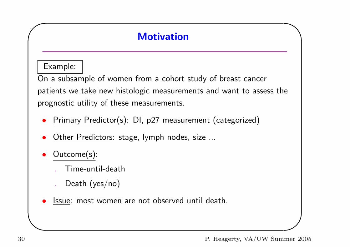
Motivation
Example:
On a subsample of women from a cohort study of breast cancer
patients we take new histologic measurements and want to assess the
prognostic utility of these measurements.
• Primary Predictor(s): DI, p27 measurement (categorized)
• Other Predictors: stage, lymph nodes, size ...
• Outcome(s):
. Time-until-death
. Death (yes/no)
• Issue: most women are not observed until death.
30 P. Heagerty, VA/UW Summer 2005
'
&
$
%
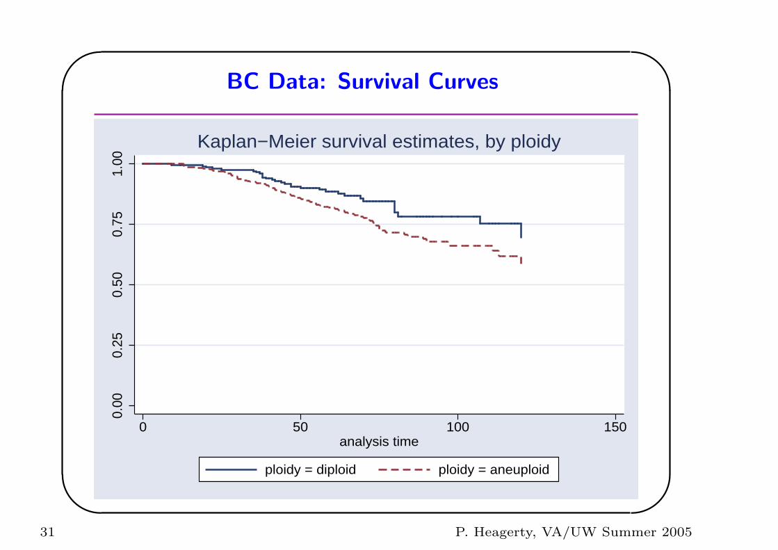
BC Data: Survival Curves
0.00
0.25
0.50
0.75
1.00
0 50 100 150analysis time
ploidy = diploid ploidy = aneuploid
Kaplan−Meier survival estimates, by ploidy
31 P. Heagerty, VA/UW Summer 2005
'
&
$
%
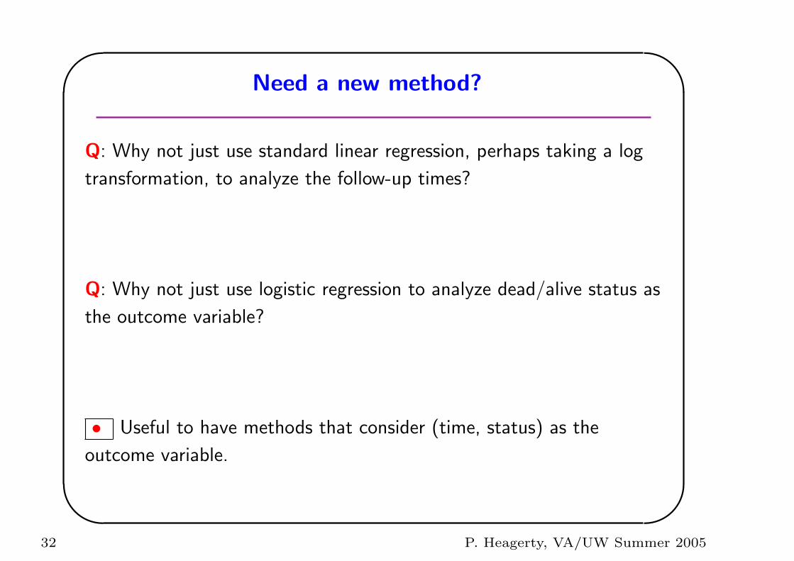
Need a new method?
Q: Why not just use standard linear regression, perhaps taking a log
transformation, to analyze the follow-up times?
Q: Why not just use logistic regression to analyze dead/alive status as
the outcome variable?
• Useful to have methods that consider (time, status) as the
outcome variable.
32 P. Heagerty, VA/UW Summer 2005
'
&
$
%
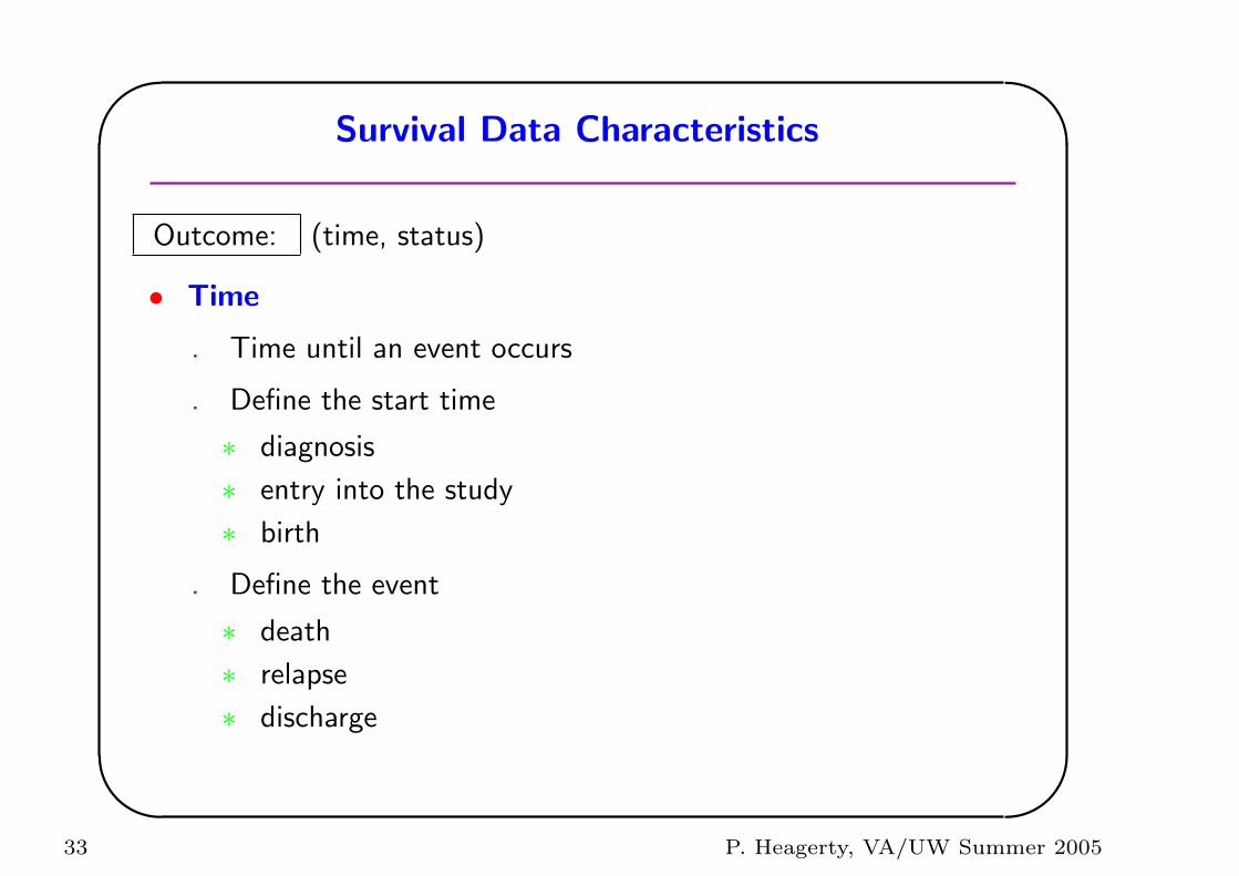
Survival Data Characteristics
Outcome: (time, status)
• Time
. Time until an event occurs
. Define the start time
∗ diagnosis
∗ entry into the study
∗ birth
. Define the event
∗ death
∗ relapse
∗ discharge
33 P. Heagerty, VA/UW Summer 2005
'
&
$
%
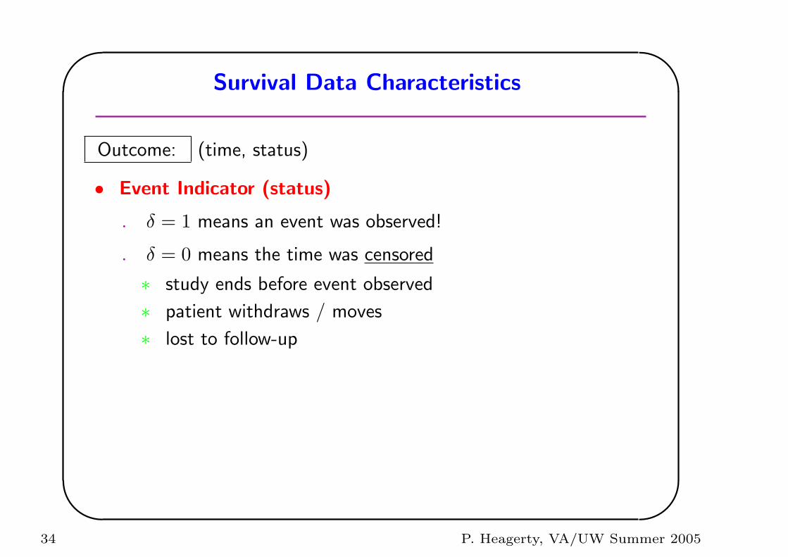
Survival Data Characteristics
Outcome: (time, status)
• Event Indicator (status)
. δ = 1 means an event was observed!
. δ = 0 means the time was censored
∗ study ends before event observed
∗ patient withdraws / moves
∗ lost to follow-up
34 P. Heagerty, VA/UW Summer 2005
'
&
$
%
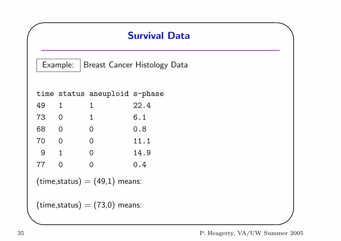
Survival Data
Example: Breast Cancer Histology Data
time status aneuploid s-phase
49 1 1 22.4
73 0 1 6.1
68 0 0 0.8
70 0 0 11.1
9 1 0 14.9
77 0 0 0.4
(time,status) = (49,1) means:
(time,status) = (73,0) means:
35 P. Heagerty, VA/UW Summer 2005
'
&
$
%
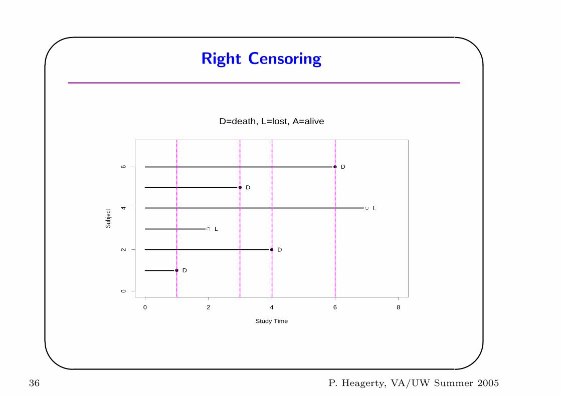
Right Censoring
Study Time
Sub
ject
0 2 4 6 8
02
46
D
D
D
D
L
L
D=death, L=lost, A=alive
36 P. Heagerty, VA/UW Summer 2005
'
&
$
%
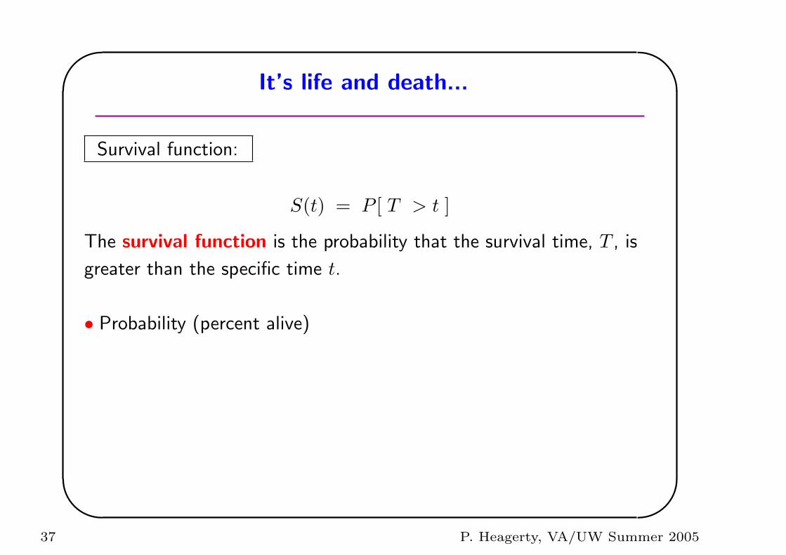
It’s life and death...
Survival function:
S(t) = P [ T > t ]
The survival function is the probability that the survival time, T , is
greater than the specific time t.
• Probability (percent alive)
37 P. Heagerty, VA/UW Summer 2005
'
&
$
%
It’s life and death...
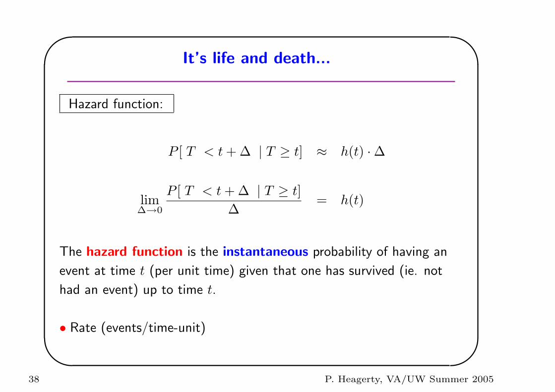
Hazard function:
P [ T < t + ∆ | T ≥ t] ≈ h(t) ·∆
lim∆→0
P [ T < t + ∆ | T ≥ t]∆
= h(t)
The hazard function is the instantaneous probability of having an
event at time t (per unit time) given that one has survived (ie. not
had an event) up to time t.
• Rate (events/time-unit)
38 P. Heagerty, VA/UW Summer 2005
'
&
$
%
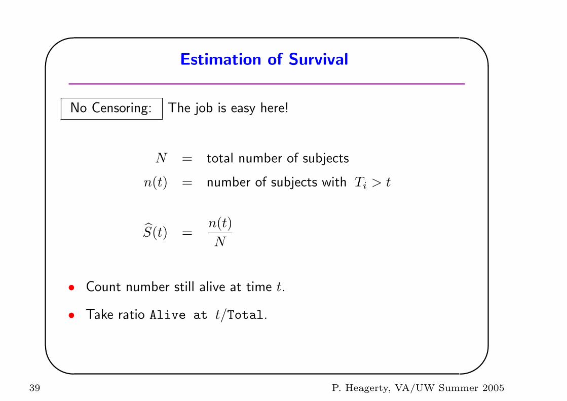
Estimation of Survival
No Censoring: The job is easy here!
N = total number of subjects
n(t) = number of subjects with Ti > t
S(t) =n(t)N
• Count number still alive at time t.
• Take ratio Alive at t/Total.
39 P. Heagerty, VA/UW Summer 2005

'
&
$
%
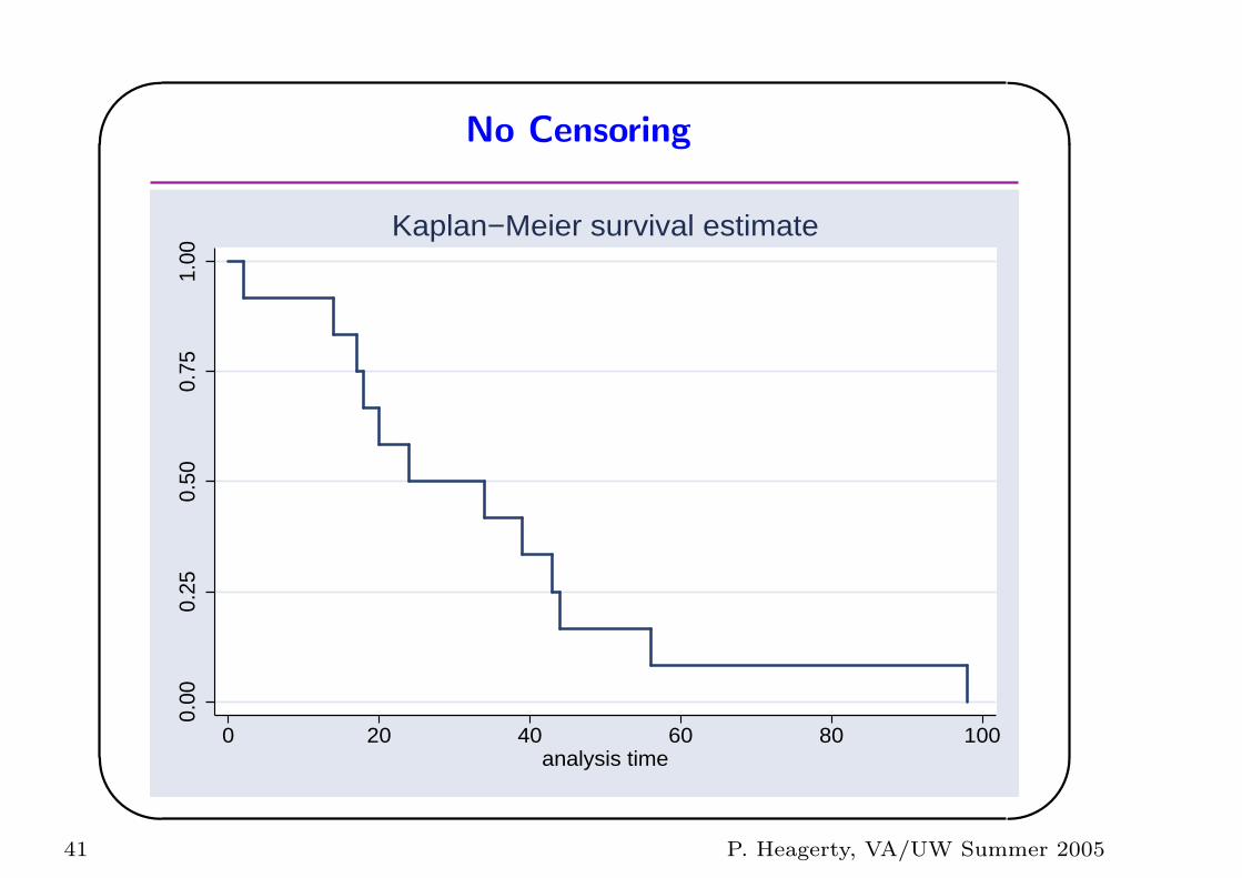
Example: Estimation of Survival
No Censoring:
N = 12 Median = 29
Quartiles = 17.5, 43.5
Decimal point is 1 place to the right of the colon
0 : 2
1 : 478
2 : 04
3 : 49
4 : 34
5 : 6
High: 98
40 P. Heagerty, VA/UW Summer 2005
'
&
$
%
No Censoring
0.00
0.25
0.50
0.75
1.00
0 20 40 60 80 100analysis time
Kaplan−Meier survival estimate
41 P. Heagerty, VA/UW Summer 2005
'
&
$
%
Survival with Censoring
Q: How can we include information from observations like 25+ which
we represent as (25,0)?
A: The Kaplan-Meier Estimator.
Before we get to the details of the Kaplan-Meier estimator we’ll want
to consider an example from current life tables that shows us how we
can “piece together” survival information.
42 P. Heagerty, VA/UW Summer 2005
'
&
$
%
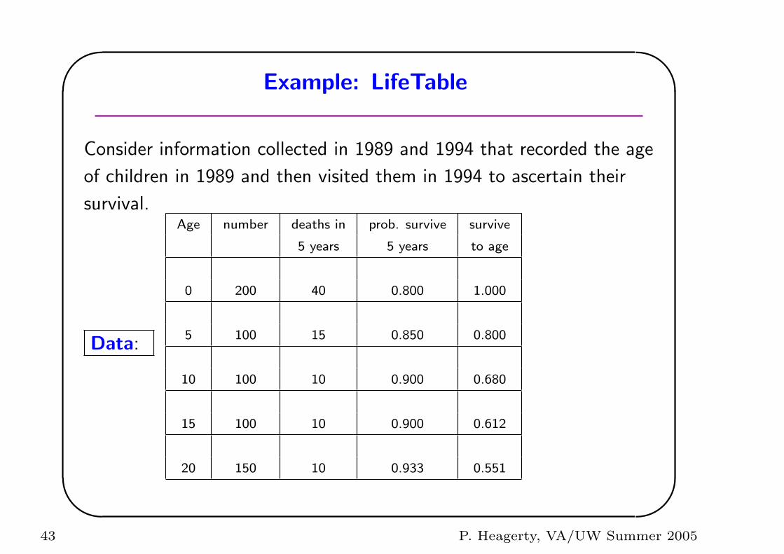
Example: LifeTable
Consider information collected in 1989 and 1994 that recorded the age
of children in 1989 and then visited them in 1994 to ascertain their
survival.
Data:
Age number deaths in prob. survive survive
5 years 5 years to age
0 200 40 0.800 1.000
5 100 15 0.850 0.800
10 100 10 0.900 0.680
15 100 10 0.900 0.612
20 150 10 0.933 0.551
43 P. Heagerty, VA/UW Summer 2005
'
&
$
%
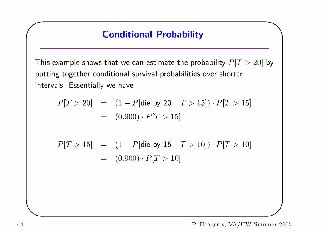
Conditional Probability
This example shows that we can estimate the probability P [T > 20] by
putting together conditional survival probabilities over shorter
intervals. Essentially we have
P [T > 20] = (1− P [die by 20 | T > 15]) · P [T > 15]
= (0.900) · P [T > 15]
P [T > 15] = (1− P [die by 15 | T > 10]) · P [T > 10]
= (0.900) · P [T > 10]
44 P. Heagerty, VA/UW Summer 2005
'
&
$
%
Conditional Probability
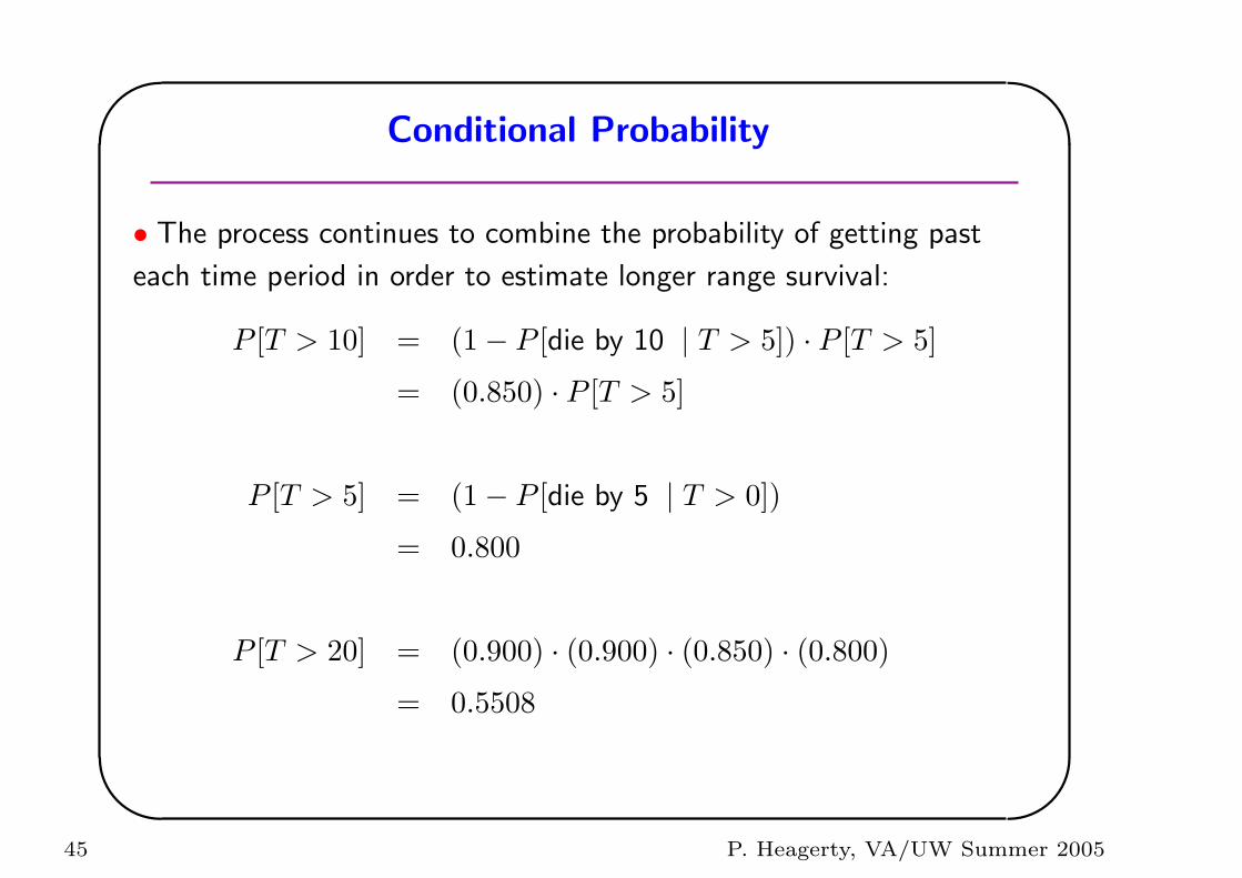
• The process continues to combine the probability of getting past
each time period in order to estimate longer range survival:
P [T > 10] = (1− P [die by 10 | T > 5]) · P [T > 5]
= (0.850) · P [T > 5]
P [T > 5] = (1− P [die by 5 | T > 0])
= 0.800
P [T > 20] = (0.900) · (0.900) · (0.850) · (0.800)
= 0.5508
45 P. Heagerty, VA/UW Summer 2005
'
&
$
%
Continuation Probabilities
We can diagram the previous calculations:
46 P. Heagerty, VA/UW Summer 2005
'
&
$
%
Kaplan-Meier Estimator
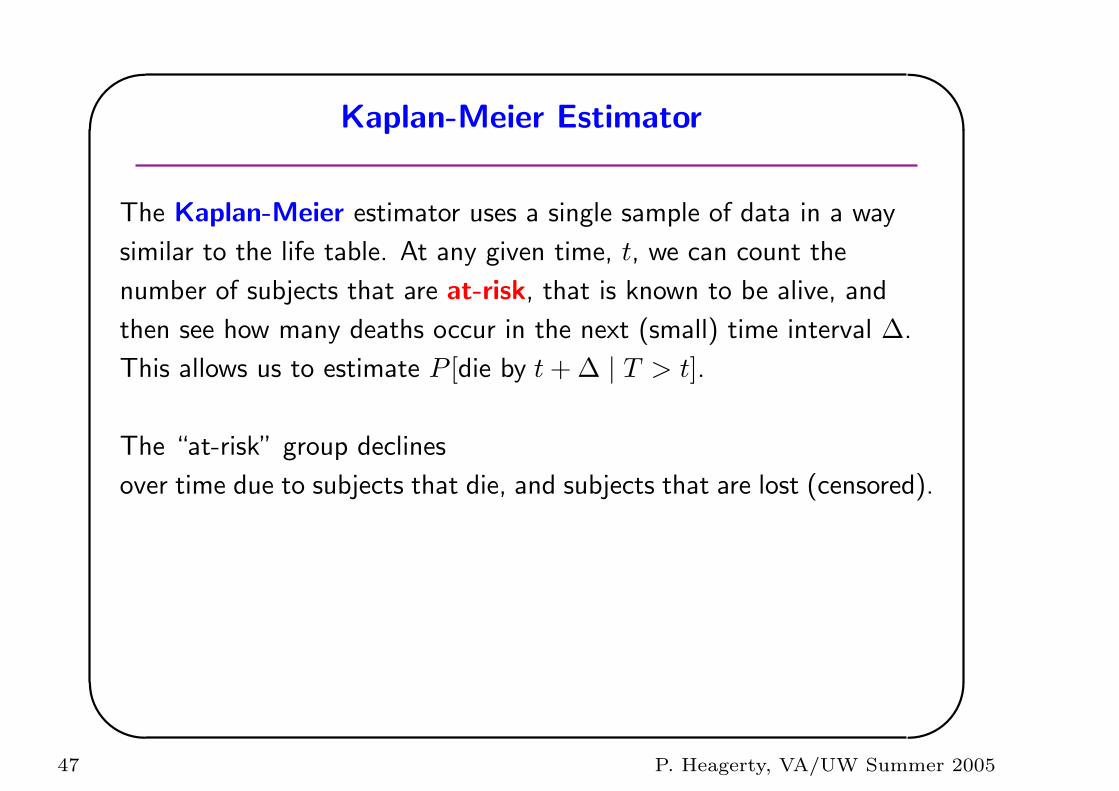
The Kaplan-Meier estimator uses a single sample of data in a way
similar to the life table. At any given time, t, we can count the
number of subjects that are at-risk, that is known to be alive, and
then see how many deaths occur in the next (small) time interval ∆.
This allows us to estimate P [die by t + ∆ | T > t].
The “at-risk” group declines
over time due to subjects that die, and subjects that are lost (censored).
47 P. Heagerty, VA/UW Summer 2005
'
&
$
%
Kaplan-Meier Estimator
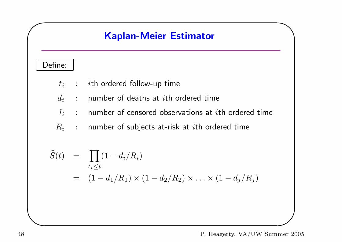
Define:
ti : ith ordered follow-up time
di : number of deaths at ith ordered time
li : number of censored observations at ith ordered time
Ri : number of subjects at-risk at ith ordered time
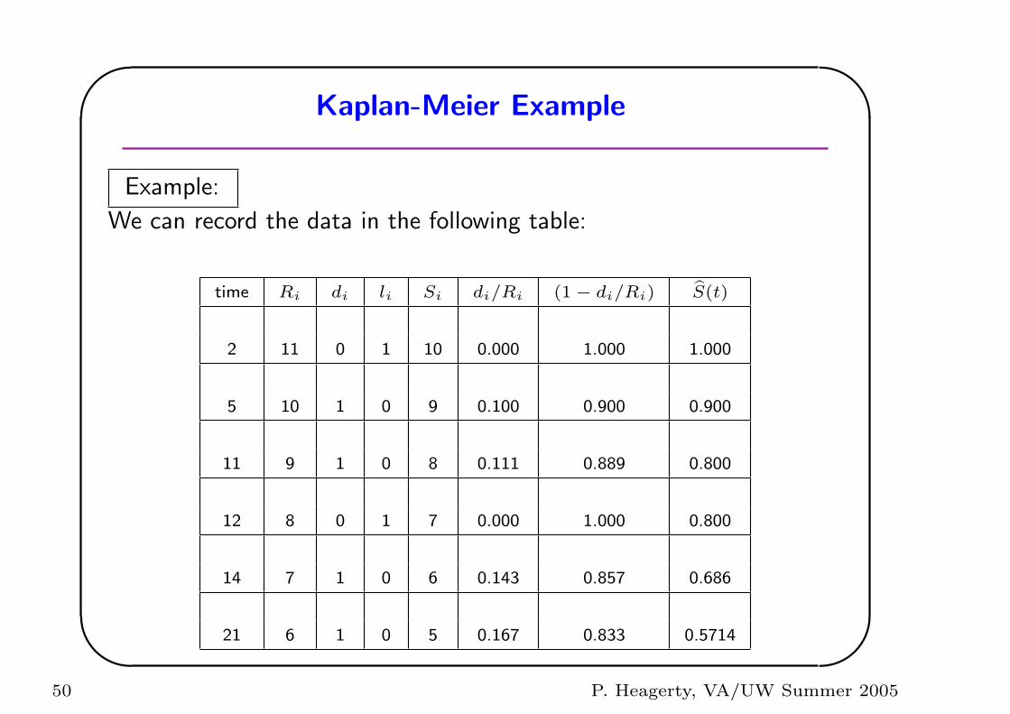
S(t) =∏
ti≤t
(1− di/Ri)
= (1− d1/R1)× (1− d2/R2)× . . .× (1− dj/Rj)
48 P. Heagerty, VA/UW Summer 2005
'
&
$
%
Kaplan-Meier Example
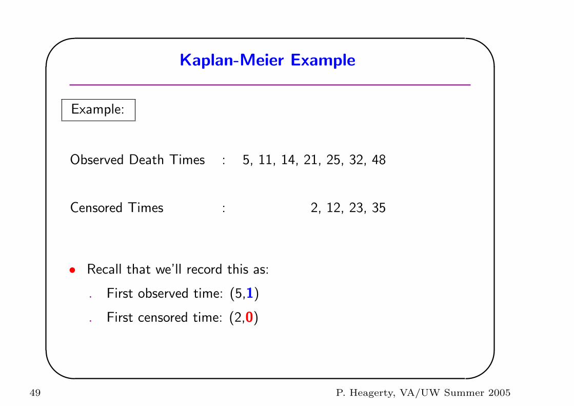
Example:
Observed Death Times : 5, 11, 14, 21, 25, 32, 48
Censored Times : 2, 12, 23, 35
• Recall that we’ll record this as:
. First observed time: (5,1)
. First censored time: (2,0)
49 P. Heagerty, VA/UW Summer 2005
'
&
$
%
Kaplan-Meier Example
Example:
We can record the data in the following table:
time Ri di li Si di/Ri (1− di/Ri) S(t)
2 11 0 1 10 0.000 1.000 1.000
5 10 1 0 9 0.100 0.900 0.900
11 9 1 0 8 0.111 0.889 0.800
12 8 0 1 7 0.000 1.000 0.800
14 7 1 0 6 0.143 0.857 0.686
21 6 1 0 5 0.167 0.833 0.5714
50 P. Heagerty, VA/UW Summer 2005
'
&
$
%
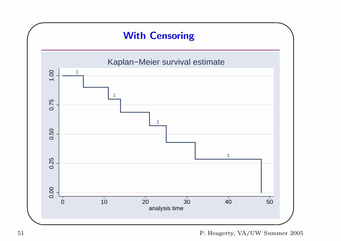
With Censoring
1
1
1
1
0.00
0.25
0.50
0.75
1.00
0 10 20 30 40 50analysis time
Kaplan−Meier survival estimate
51 P. Heagerty, VA/UW Summer 2005
'
&
$
%
Summary
1. “Time-until” outcomes (survival times) are common in biomedical
research.
2. Survival times are often right-skewed.
3. Often a fraction of the times are right-censored.
4. The Kaplan-Meier estimator can be used to estimate and display
the distribution of survival times.
5. Life tables are used to combine information across age groups.
52 P. Heagerty, VA/UW Summer 2005
'
&
$
%
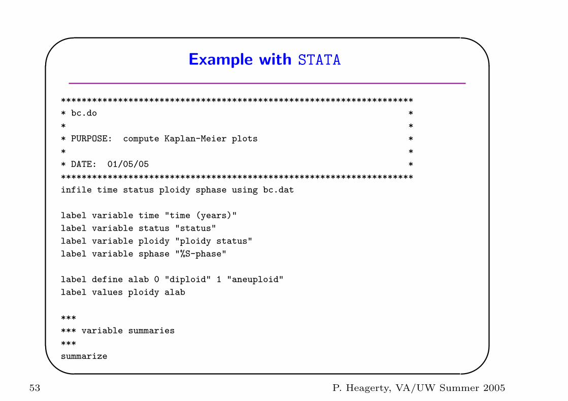
Example with STATA
********************************************************************
* bc.do *
* *
* PURPOSE: compute Kaplan-Meier plots *
* *
* DATE: 01/05/05 *
********************************************************************
infile time status ploidy sphase using bc.dat
label variable time "time (years)"
label variable status "status"
label variable ploidy "ploidy status"
label variable sphase "%S-phase"
label define alab 0 "diploid" 1 "aneuploid"
label values ploidy alab
***
*** variable summaries
***
summarize
53 P. Heagerty, VA/UW Summer 2005
'
&
$
%
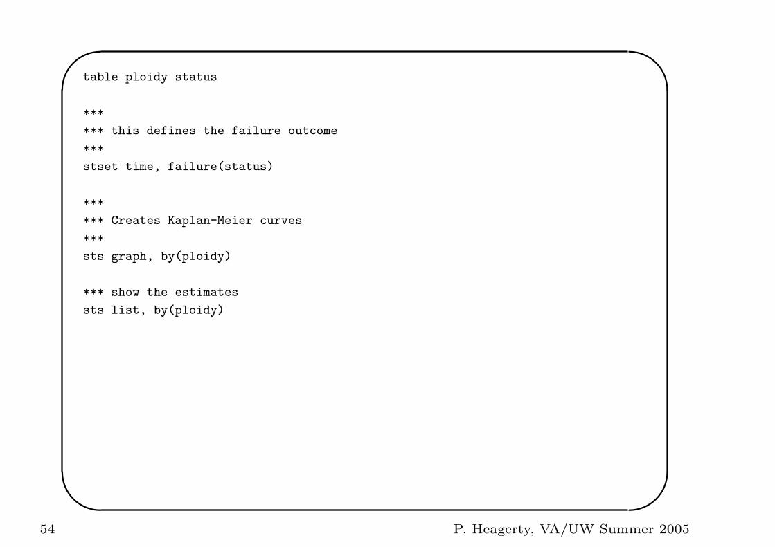
table ploidy status
***
*** this defines the failure outcome
***
stset time, failure(status)
***
*** Creates Kaplan-Meier curves
***
sts graph, by(ploidy)
*** show the estimates
sts list, by(ploidy)
54 P. Heagerty, VA/UW Summer 2005
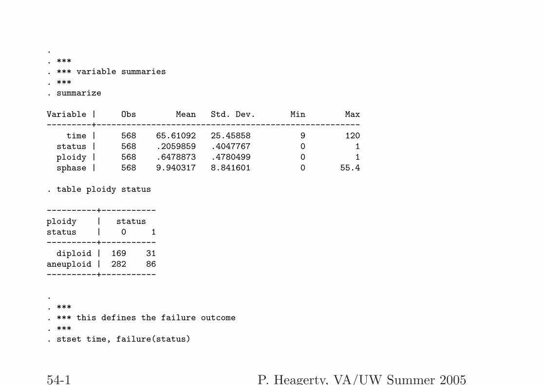
.
. ***
. *** variable summaries
. ***
. summarize
Variable | Obs Mean Std. Dev. Min Max---------+-----------------------------------------------------
time | 568 65.61092 25.45858 9 120status | 568 .2059859 .4047767 0 1ploidy | 568 .6478873 .4780499 0 1sphase | 568 9.940317 8.841601 0 55.4
. table ploidy status
----------+-----------ploidy | statusstatus | 0 1----------+-----------
diploid | 169 31aneuploid | 282 86----------+-----------
.
. ***
. *** this defines the failure outcome
. ***
. stset time, failure(status)
54-1 P. Heagerty, VA/UW Summer 2005
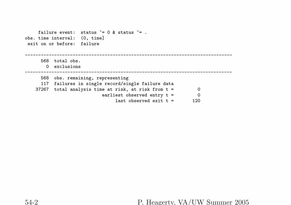
failure event: status ~= 0 & status ~= .obs. time interval: (0, time]exit on or before: failure
------------------------------------------------------------------------------568 total obs.
0 exclusions------------------------------------------------------------------------------
568 obs. remaining, representing117 failures in single record/single failure data
37267 total analysis time at risk, at risk from t = 0earliest observed entry t = 0
last observed exit t = 120
54-2 P. Heagerty, VA/UW Summer 2005
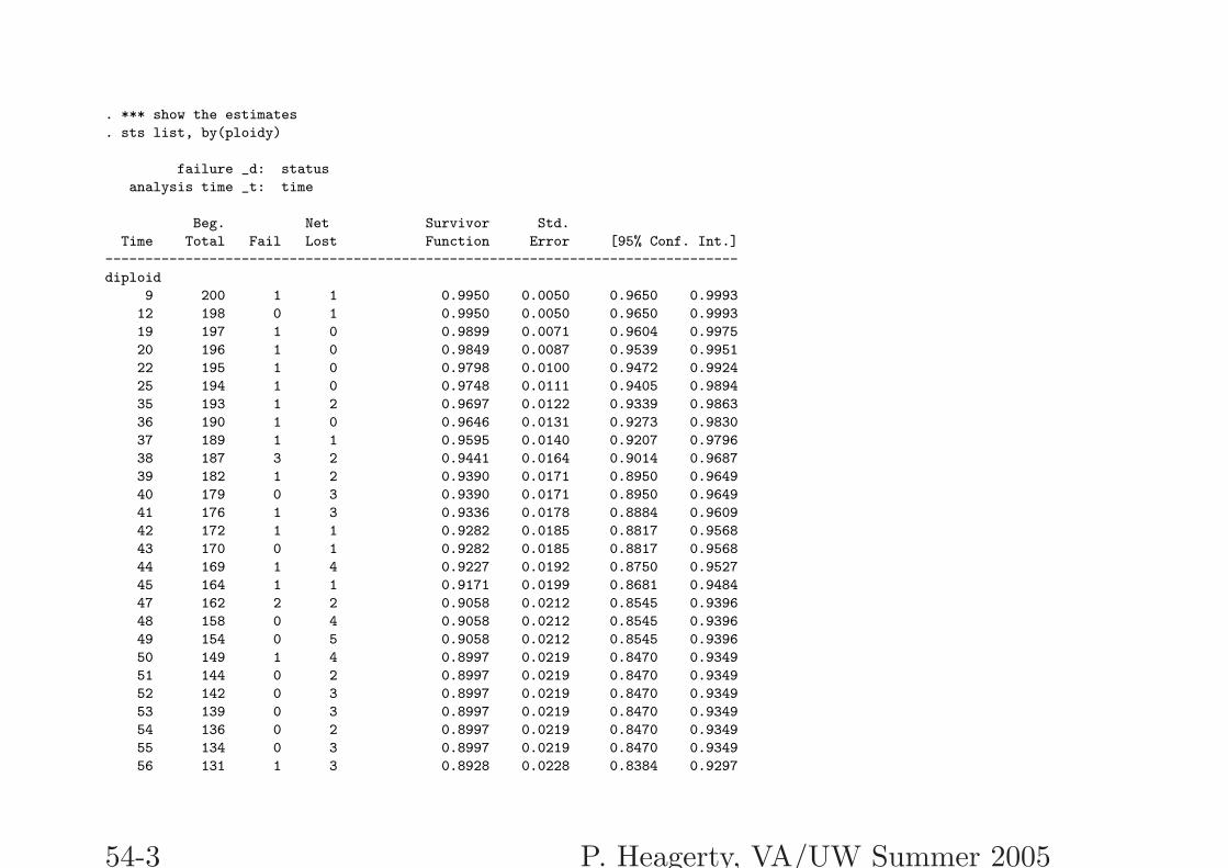
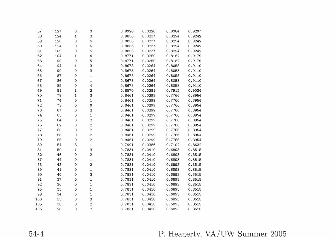
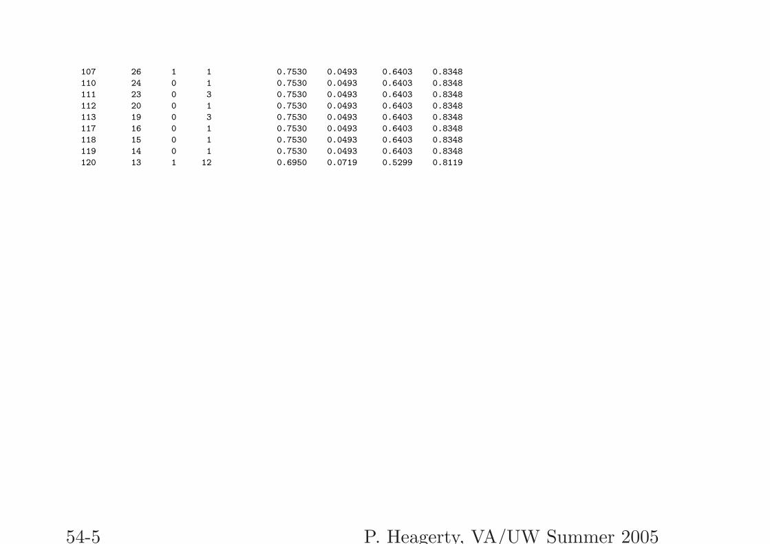
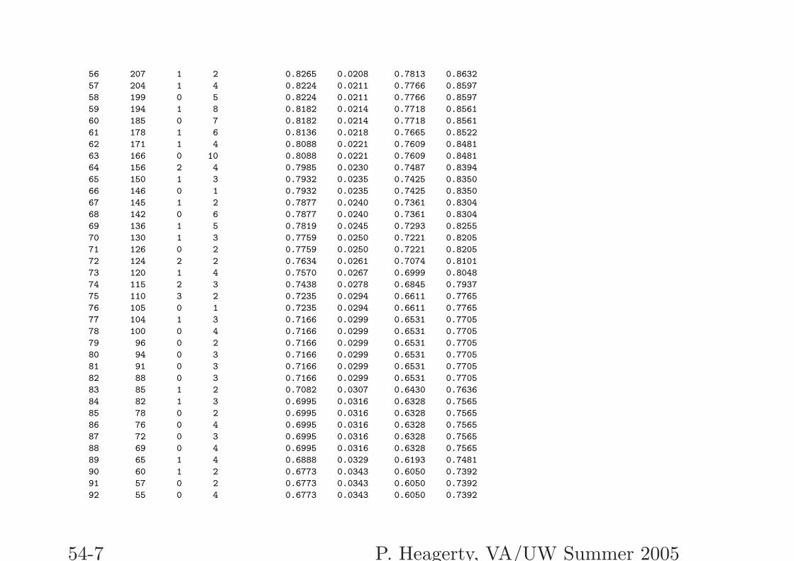
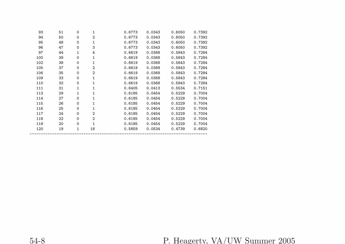
. *** show the estimates
. sts list, by(ploidy)
failure _d: status
analysis time _t: time
Beg. Net Survivor Std.
Time Total Fail Lost Function Error [95% Conf. Int.]
-------------------------------------------------------------------------------
diploid
9 200 1 1 0.9950 0.0050 0.9650 0.9993
12 198 0 1 0.9950 0.0050 0.9650 0.9993
19 197 1 0 0.9899 0.0071 0.9604 0.9975
20 196 1 0 0.9849 0.0087 0.9539 0.9951
22 195 1 0 0.9798 0.0100 0.9472 0.9924
25 194 1 0 0.9748 0.0111 0.9405 0.9894
35 193 1 2 0.9697 0.0122 0.9339 0.9863
36 190 1 0 0.9646 0.0131 0.9273 0.9830
37 189 1 1 0.9595 0.0140 0.9207 0.9796
38 187 3 2 0.9441 0.0164 0.9014 0.9687
39 182 1 2 0.9390 0.0171 0.8950 0.9649
40 179 0 3 0.9390 0.0171 0.8950 0.9649
41 176 1 3 0.9336 0.0178 0.8884 0.9609
42 172 1 1 0.9282 0.0185 0.8817 0.9568
43 170 0 1 0.9282 0.0185 0.8817 0.9568
44 169 1 4 0.9227 0.0192 0.8750 0.9527
45 164 1 1 0.9171 0.0199 0.8681 0.9484
47 162 2 2 0.9058 0.0212 0.8545 0.9396
48 158 0 4 0.9058 0.0212 0.8545 0.9396
49 154 0 5 0.9058 0.0212 0.8545 0.9396
50 149 1 4 0.8997 0.0219 0.8470 0.9349
51 144 0 2 0.8997 0.0219 0.8470 0.9349
52 142 0 3 0.8997 0.0219 0.8470 0.9349
53 139 0 3 0.8997 0.0219 0.8470 0.9349
54 136 0 2 0.8997 0.0219 0.8470 0.9349
55 134 0 3 0.8997 0.0219 0.8470 0.9349
56 131 1 3 0.8928 0.0228 0.8384 0.9297
54-3 P. Heagerty, VA/UW Summer 2005
57 127 0 3 0.8928 0.0228 0.8384 0.9297
58 124 1 3 0.8856 0.0237 0.8294 0.9242
59 120 0 6 0.8856 0.0237 0.8294 0.9242
60 114 0 5 0.8856 0.0237 0.8294 0.9242
61 109 0 5 0.8856 0.0237 0.8294 0.9242
62 104 1 4 0.8771 0.0250 0.8182 0.9179
63 99 0 5 0.8771 0.0250 0.8182 0.9179
64 94 1 3 0.8678 0.0264 0.8058 0.9110
65 90 0 3 0.8678 0.0264 0.8058 0.9110
66 87 0 1 0.8678 0.0264 0.8058 0.9110
67 86 0 1 0.8678 0.0264 0.8058 0.9110
68 85 0 4 0.8678 0.0264 0.8058 0.9110
69 81 1 2 0.8570 0.0281 0.7912 0.9034
70 78 1 3 0.8461 0.0299 0.7766 0.8954
71 74 0 1 0.8461 0.0299 0.7766 0.8954
72 73 0 6 0.8461 0.0299 0.7766 0.8954
73 67 0 2 0.8461 0.0299 0.7766 0.8954
74 65 0 1 0.8461 0.0299 0.7766 0.8954
75 64 0 2 0.8461 0.0299 0.7766 0.8954
76 62 0 2 0.8461 0.0299 0.7766 0.8954
77 60 0 2 0.8461 0.0299 0.7766 0.8954
78 58 0 2 0.8461 0.0299 0.7766 0.8954
79 56 0 2 0.8461 0.0299 0.7766 0.8954
80 54 3 1 0.7991 0.0386 0.7102 0.8632
81 50 1 3 0.7831 0.0410 0.6893 0.8515
82 46 0 2 0.7831 0.0410 0.6893 0.8515
87 44 0 1 0.7831 0.0410 0.6893 0.8515
88 43 0 2 0.7831 0.0410 0.6893 0.8515
89 41 0 1 0.7831 0.0410 0.6893 0.8515
90 40 0 3 0.7831 0.0410 0.6893 0.8515
91 37 0 1 0.7831 0.0410 0.6893 0.8515
92 36 0 1 0.7831 0.0410 0.6893 0.8515
95 35 0 1 0.7831 0.0410 0.6893 0.8515
98 34 0 1 0.7831 0.0410 0.6893 0.8515
100 33 0 3 0.7831 0.0410 0.6893 0.8515
105 30 0 2 0.7831 0.0410 0.6893 0.8515
106 28 0 2 0.7831 0.0410 0.6893 0.8515
54-4 P. Heagerty, VA/UW Summer 2005
107 26 1 1 0.7530 0.0493 0.6403 0.8348
110 24 0 1 0.7530 0.0493 0.6403 0.8348
111 23 0 3 0.7530 0.0493 0.6403 0.8348
112 20 0 1 0.7530 0.0493 0.6403 0.8348
113 19 0 3 0.7530 0.0493 0.6403 0.8348
117 16 0 1 0.7530 0.0493 0.6403 0.8348
118 15 0 1 0.7530 0.0493 0.6403 0.8348
119 14 0 1 0.7530 0.0493 0.6403 0.8348
120 13 1 12 0.6950 0.0719 0.5299 0.8119
54-5 P. Heagerty, VA/UW Summer 2005
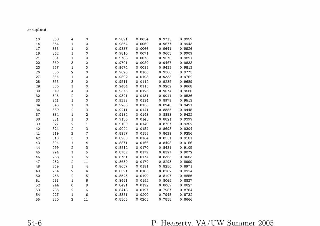
aneuploid
13 368 4 0 0.9891 0.0054 0.9713 0.9959
14 364 1 0 0.9864 0.0060 0.9677 0.9943
17 363 1 0 0.9837 0.0066 0.9641 0.9926
19 362 1 0 0.9810 0.0071 0.9605 0.9909
21 361 1 0 0.9783 0.0076 0.9570 0.9891
22 360 3 0 0.9701 0.0089 0.9467 0.9833
23 357 1 0 0.9674 0.0093 0.9433 0.9813
26 356 2 0 0.9620 0.0100 0.9366 0.9773
27 354 1 0 0.9592 0.0103 0.9333 0.9752
28 353 3 0 0.9511 0.0112 0.9235 0.9689
29 350 1 0 0.9484 0.0115 0.9202 0.9668
30 349 4 0 0.9375 0.0126 0.9074 0.9580
32 345 2 2 0.9321 0.0131 0.9011 0.9536
33 341 1 0 0.9293 0.0134 0.8979 0.9513
34 340 1 0 0.9266 0.0136 0.8948 0.9491
36 339 2 3 0.9211 0.0141 0.8885 0.9445
37 334 1 2 0.9184 0.0143 0.8853 0.9422
38 331 1 3 0.9156 0.0145 0.8821 0.9399
39 327 2 1 0.9100 0.0149 0.8757 0.9352
40 324 2 3 0.9044 0.0154 0.8693 0.9304
41 319 2 7 0.8987 0.0158 0.8629 0.9256
42 310 3 3 0.8900 0.0164 0.8531 0.9181
43 304 1 4 0.8871 0.0166 0.8498 0.9156
44 299 2 3 0.8812 0.0170 0.8431 0.9105
45 294 1 5 0.8782 0.0172 0.8397 0.9079
46 288 1 5 0.8751 0.0174 0.8363 0.9053
47 282 2 11 0.8689 0.0179 0.8293 0.8999
48 269 1 4 0.8657 0.0181 0.8256 0.8971
49 264 2 4 0.8591 0.0185 0.8182 0.8914
50 258 2 5 0.8525 0.0190 0.8107 0.8856
51 251 1 6 0.8491 0.0192 0.8069 0.8827
52 244 0 9 0.8491 0.0192 0.8069 0.8827
53 235 2 6 0.8418 0.0197 0.7987 0.8764
54 227 1 6 0.8381 0.0200 0.7945 0.8732
55 220 2 11 0.8305 0.0205 0.7858 0.8666
54-6 P. Heagerty, VA/UW Summer 2005
56 207 1 2 0.8265 0.0208 0.7813 0.8632
57 204 1 4 0.8224 0.0211 0.7766 0.8597
58 199 0 5 0.8224 0.0211 0.7766 0.8597
59 194 1 8 0.8182 0.0214 0.7718 0.8561
60 185 0 7 0.8182 0.0214 0.7718 0.8561
61 178 1 6 0.8136 0.0218 0.7665 0.8522
62 171 1 4 0.8088 0.0221 0.7609 0.8481
63 166 0 10 0.8088 0.0221 0.7609 0.8481
64 156 2 4 0.7985 0.0230 0.7487 0.8394
65 150 1 3 0.7932 0.0235 0.7425 0.8350
66 146 0 1 0.7932 0.0235 0.7425 0.8350
67 145 1 2 0.7877 0.0240 0.7361 0.8304
68 142 0 6 0.7877 0.0240 0.7361 0.8304
69 136 1 5 0.7819 0.0245 0.7293 0.8255
70 130 1 3 0.7759 0.0250 0.7221 0.8205
71 126 0 2 0.7759 0.0250 0.7221 0.8205
72 124 2 2 0.7634 0.0261 0.7074 0.8101
73 120 1 4 0.7570 0.0267 0.6999 0.8048
74 115 2 3 0.7438 0.0278 0.6845 0.7937
75 110 3 2 0.7235 0.0294 0.6611 0.7765
76 105 0 1 0.7235 0.0294 0.6611 0.7765
77 104 1 3 0.7166 0.0299 0.6531 0.7705
78 100 0 4 0.7166 0.0299 0.6531 0.7705
79 96 0 2 0.7166 0.0299 0.6531 0.7705
80 94 0 3 0.7166 0.0299 0.6531 0.7705
81 91 0 3 0.7166 0.0299 0.6531 0.7705
82 88 0 3 0.7166 0.0299 0.6531 0.7705
83 85 1 2 0.7082 0.0307 0.6430 0.7636
84 82 1 3 0.6995 0.0316 0.6328 0.7565
85 78 0 2 0.6995 0.0316 0.6328 0.7565
86 76 0 4 0.6995 0.0316 0.6328 0.7565
87 72 0 3 0.6995 0.0316 0.6328 0.7565
88 69 0 4 0.6995 0.0316 0.6328 0.7565
89 65 1 4 0.6888 0.0329 0.6193 0.7481
90 60 1 2 0.6773 0.0343 0.6050 0.7392
91 57 0 2 0.6773 0.0343 0.6050 0.7392
92 55 0 4 0.6773 0.0343 0.6050 0.7392
54-7 P. Heagerty, VA/UW Summer 2005
93 51 0 1 0.6773 0.0343 0.6050 0.7392
94 50 0 2 0.6773 0.0343 0.6050 0.7392
95 48 0 1 0.6773 0.0343 0.6050 0.7392
96 47 0 3 0.6773 0.0343 0.6050 0.7392
97 44 1 4 0.6619 0.0368 0.5843 0.7284
100 39 0 1 0.6619 0.0368 0.5843 0.7284
102 38 0 1 0.6619 0.0368 0.5843 0.7284
105 37 0 2 0.6619 0.0368 0.5843 0.7284
106 35 0 2 0.6619 0.0368 0.5843 0.7284
109 33 0 1 0.6619 0.0368 0.5843 0.7284
110 32 0 1 0.6619 0.0368 0.5843 0.7284
111 31 1 1 0.6405 0.0413 0.5534 0.7151
113 29 1 1 0.6185 0.0454 0.5229 0.7004
114 27 0 1 0.6185 0.0454 0.5229 0.7004
115 26 0 1 0.6185 0.0454 0.5229 0.7004
116 25 0 1 0.6185 0.0454 0.5229 0.7004
117 24 0 2 0.6185 0.0454 0.5229 0.7004
118 22 0 2 0.6185 0.0454 0.5229 0.7004
119 20 0 1 0.6185 0.0454 0.5229 0.7004
120 19 1 18 0.5859 0.0534 0.4739 0.6820
-------------------------------------------------------------------------------
54-8 P. Heagerty, VA/UW Summer 2005
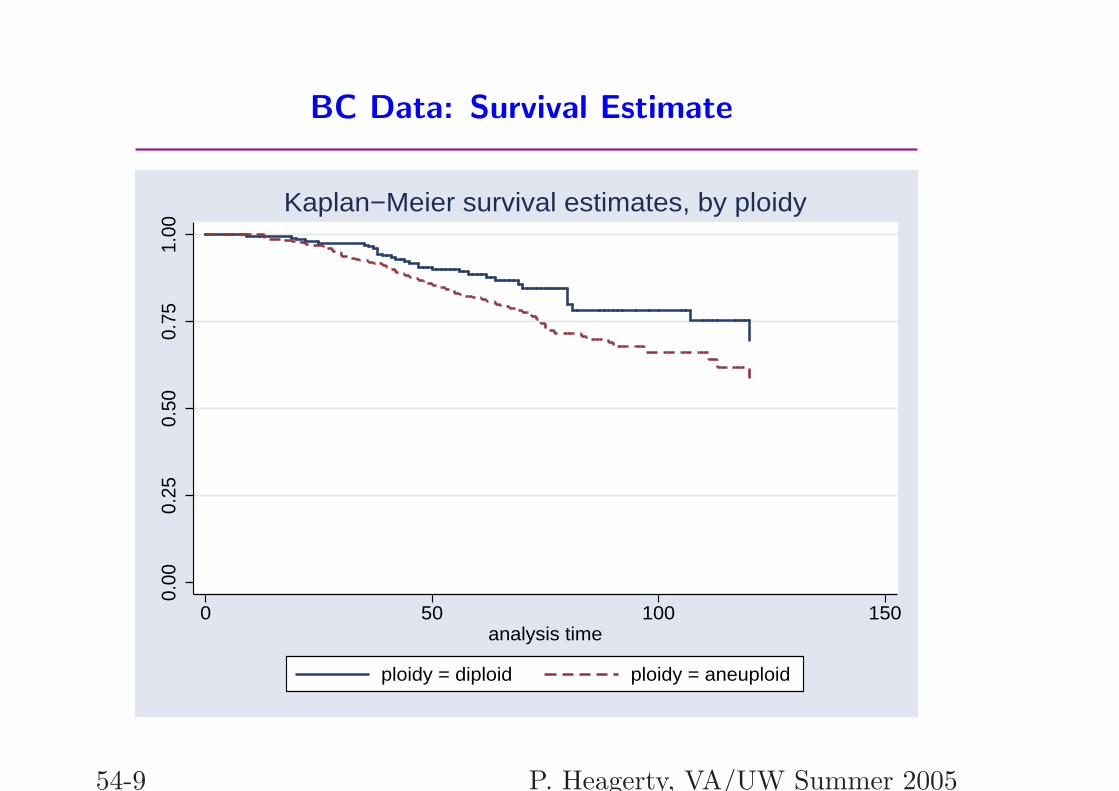
BC Data: Survival Estimate
0.00
0.25
0.50
0.75
1.00
0 50 100 150analysis time
ploidy = diploid ploidy = aneuploid
Kaplan−Meier survival estimates, by ploidy
54-9 P. Heagerty, VA/UW Summer 2005
'
&
$
%
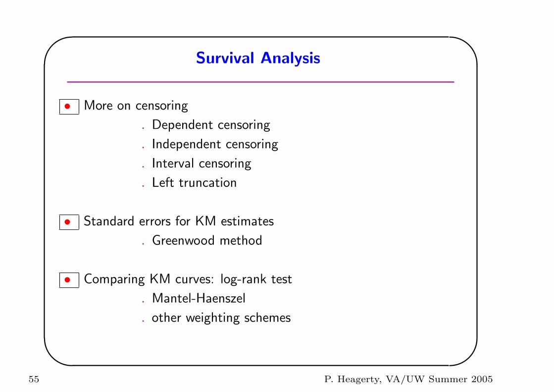
Survival Analysis
• More on censoring
. Dependent censoring
. Independent censoring
. Interval censoring
. Left truncation
• Standard errors for KM estimates
. Greenwood method
• Comparing KM curves: log-rank test
. Mantel-Haenszel
. other weighting schemes
55 P. Heagerty, VA/UW Summer 2005
'
&
$
%
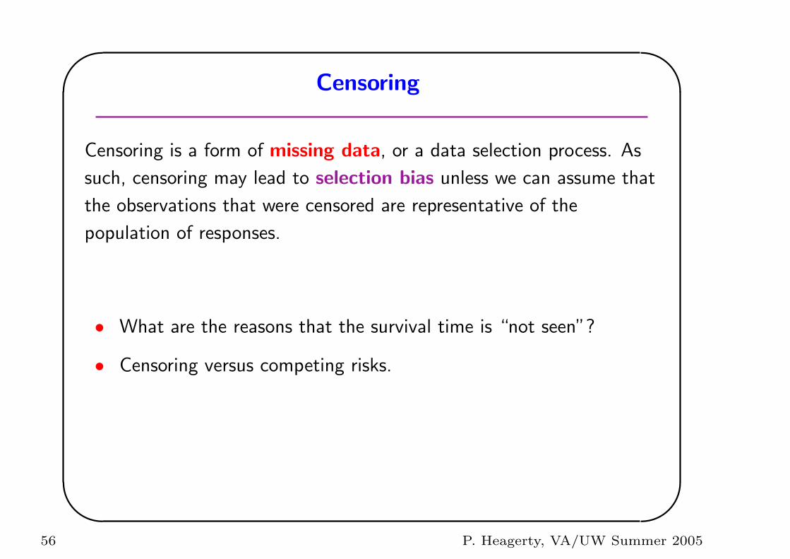
Censoring
Censoring is a form of missing data, or a data selection process. As
such, censoring may lead to selection bias unless we can assume that
the observations that were censored are representative of the
population of responses.
• What are the reasons that the survival time is “not seen”?
• Censoring versus competing risks.
56 P. Heagerty, VA/UW Summer 2005
'
&
$
%
Example:
Suppose that in a clinical trial we remove subjects from the study
when they are still alive but appear to be particularly ill (or particularly
well). If we treat these as censored and then assume that they were
representative we would obtain biased estimates of survival
probabilities, S(t).
This is an example of dependent censoring. All of the procedures
that we’ll discuss assume that the censoring is independent of the
survival times, Ti.
57 P. Heagerty, VA/UW Summer 2005
'
&
$
%
Censoring
Assumption:
Di = the survival time for subject i
Ci = the censoring time for subject i
Ti = min(Di, Ci)
δi = 1 if Di < Ci, and 0 otherwise
• We assume that the censoring time, Ci, is independent of the
survival time, Di.
58 P. Heagerty, VA/UW Summer 2005
'
&
$
%
Censoring
We observe the pair: (time = Ti, status = δi).
• Censoring due to the end of study ⇒. Independent Censoring
• Censoring due to drop-out ⇒. verify based on reasons for drop-out
• Censoring due to another type of outcome ⇒. “competing risks”, assumed independent
59 P. Heagerty, VA/UW Summer 2005
'
&
$
%
More on Censoring
Interval Censoring:
This occurs when we do not observe the exact time of failure, but
rather two time points between which the event occurred:
a ≤ Ti < b
• HIV vaccine trial with 6 monthly blood testing.
• If everyone shares the same time intervals (ie. 6 month visit
schedule) then the outcomes are known as discrete survival times, and
logistic regression methods can be used.
60 P. Heagerty, VA/UW Summer 2005
'
&
$
%
More on Censoring
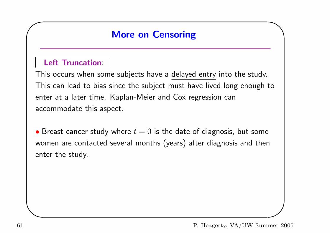
Left Truncation:
This occurs when some subjects have a delayed entry into the study.
This can lead to bias since the subject must have lived long enough to
enter at a later time. Kaplan-Meier and Cox regression can
accommodate this aspect.
• Breast cancer study where t = 0 is the date of diagnosis, but some
women are contacted several months (years) after diagnosis and then
enter the study.
61 P. Heagerty, VA/UW Summer 2005
'
&
$
%
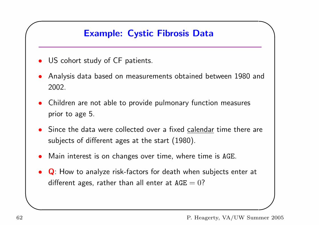
Example: Cystic Fibrosis Data
• US cohort study of CF patients.
• Analysis data based on measurements obtained between 1980 and
2002.
• Children are not able to provide pulmonary function measures
prior to age 5.
• Since the data were collected over a fixed calendar time there are
subjects of different ages at the start (1980).
• Main interest is on changes over time, where time is AGE.
• Q: How to analyze risk-factors for death when subjects enter at
different ages, rather than all enter at AGE = 0?
62 P. Heagerty, VA/UW Summer 2005
'
&
$
%
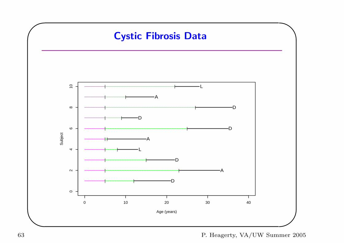
Cystic Fibrosis Data
Age (years)
Sub
ject
0 10 20 30 40
02
46
810
D| |
A| |
D| |
L| |
A| |
D| |
D| |
D| |
A| |
L| |
63 P. Heagerty, VA/UW Summer 2005
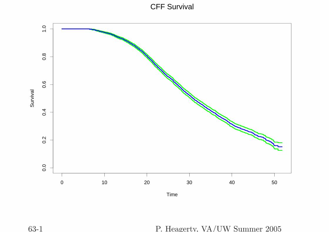
Time
Sur
viva
l
0 10 20 30 40 50
0.0
0.2
0.4
0.6
0.8
1.0
CFF Survival
63-1 P. Heagerty, VA/UW Summer 2005
'
&
$
%
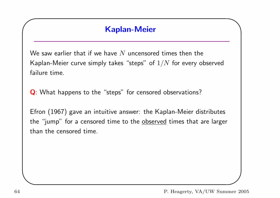
Kaplan-Meier
We saw earlier that if we have N uncensored times then the
Kaplan-Meier curve simply takes “steps” of 1/N for every observed
failure time.
Q: What happens to the “steps” for censored observations?
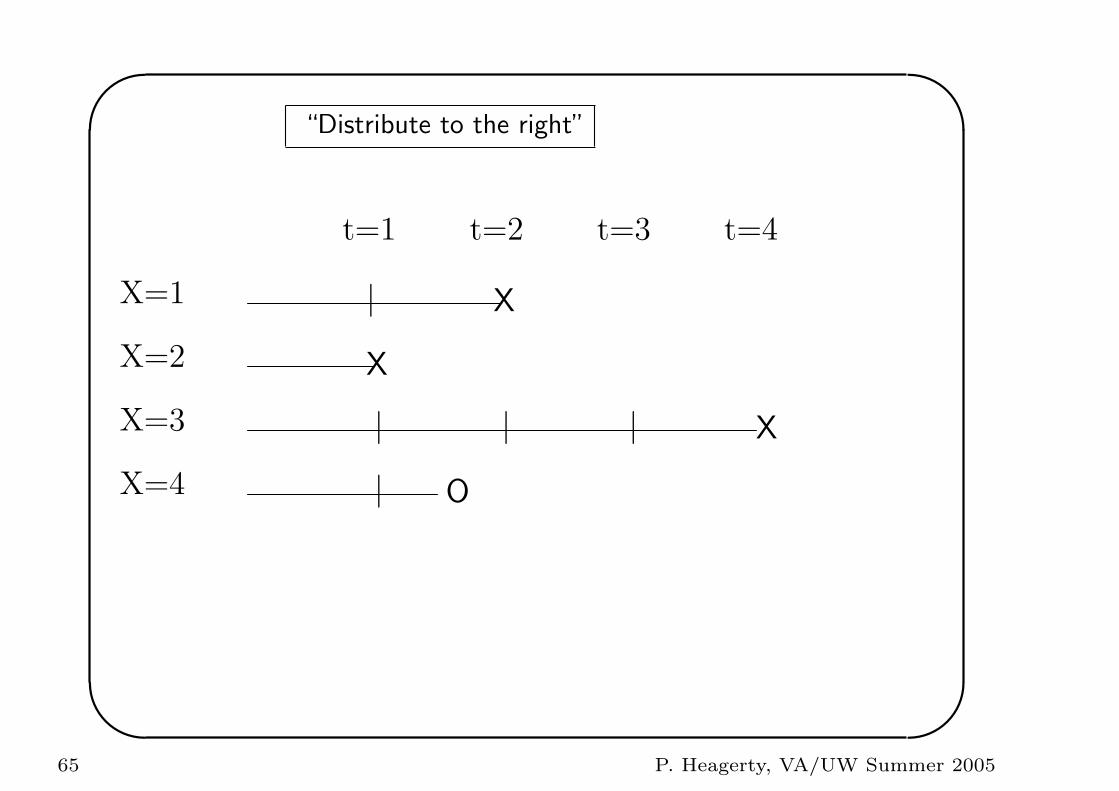
Efron (1967) gave an intuitive answer: the Kaplan-Meier distributes
the “jump” for a censored time to the observed times that are larger
than the censored time.
64 P. Heagerty, VA/UW Summer 2005
'
&
$
%
“Distribute to the right”
|
||
| | X
O
X
X
t=1 t=2 t=3 t=4
X=1
X=2
X=3
X=4
65 P. Heagerty, VA/UW Summer 2005
'
&
$
%
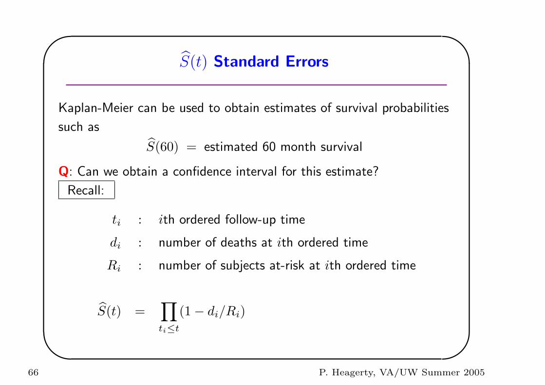
S(t) Standard Errors
Kaplan-Meier can be used to obtain estimates of survival probabilities
such as
S(60) = estimated 60 month survival
Q: Can we obtain a confidence interval for this estimate?
Recall:
ti : ith ordered follow-up time
di : number of deaths at ith ordered time
Ri : number of subjects at-risk at ith ordered time
S(t) =∏
ti≤t
(1− di/Ri)
66 P. Heagerty, VA/UW Summer 2005
'
&
$
%
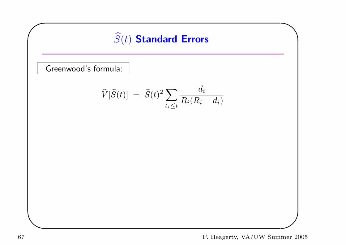
S(t) Standard Errors
Greenwood’s formula:
V [S(t)] = S(t)2∑
ti≤t
di
Ri(Ri − di)
67 P. Heagerty, VA/UW Summer 2005
'
&
$
%
S(t) Standard Errors
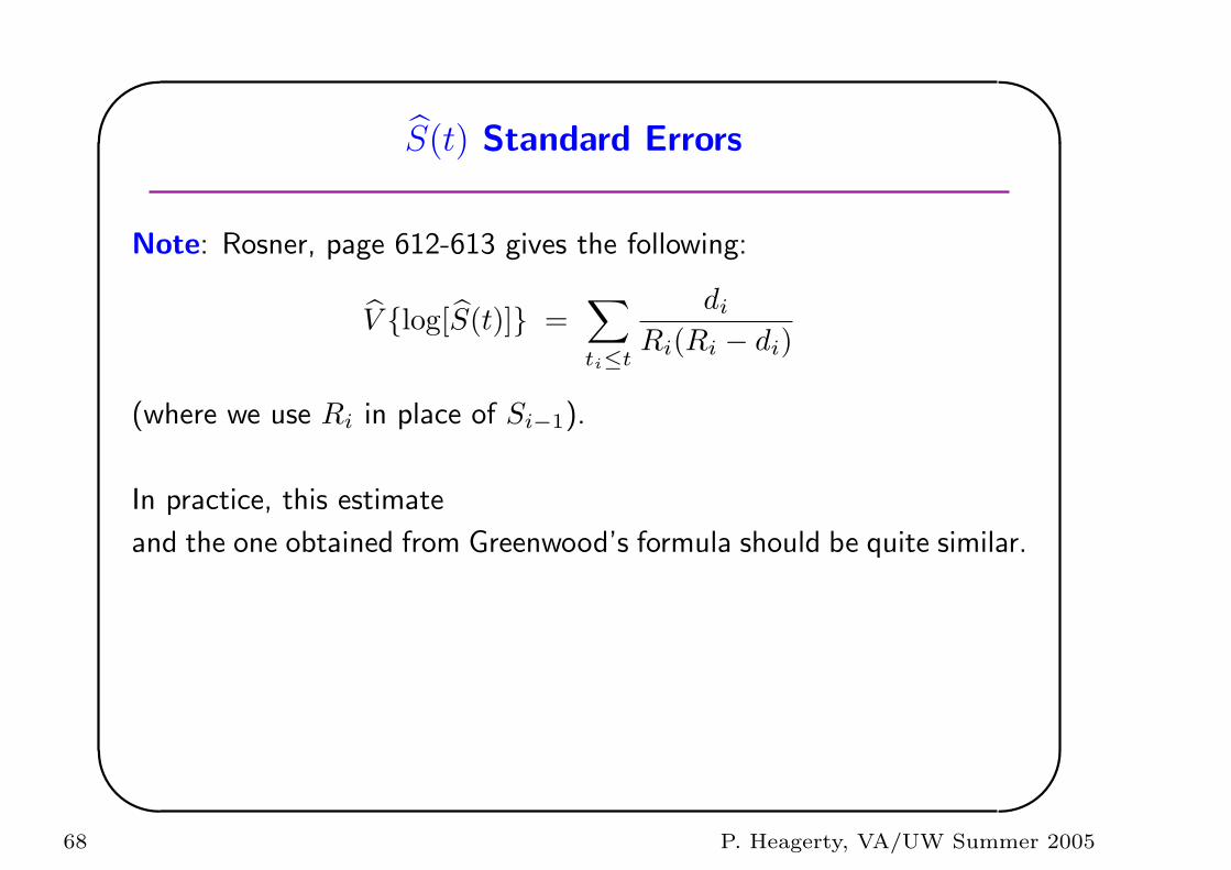
Note: Rosner, page 612-613 gives the following:
V {log[S(t)]} =∑
ti≤t
di
Ri(Ri − di)
(where we use Ri in place of Si−1).
In practice, this estimate
and the one obtained from Greenwood’s formula should be quite similar.
68 P. Heagerty, VA/UW Summer 2005
'
&
$
%
S(t) Standard Errors
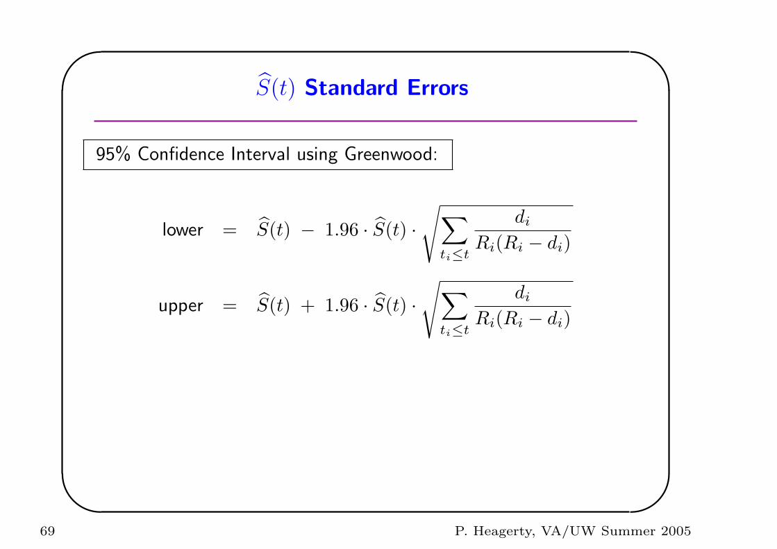
95% Confidence Interval using Greenwood:
lower = S(t) − 1.96 · S(t) ·√∑
ti≤t
di
Ri(Ri − di)
upper = S(t) + 1.96 · S(t) ·√∑
ti≤t
di
Ri(Ri − di)
69 P. Heagerty, VA/UW Summer 2005
'
&
$
%
Computing S(t) Standard Errors
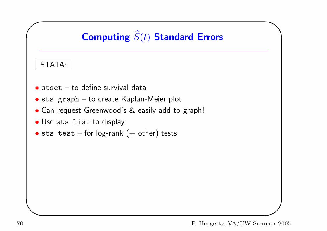
STATA:
• stset – to define survival data
• sts graph – to create Kaplan-Meier plot
• Can request Greenwood’s & easily add to graph!
• Use sts list to display.
• sts test – for log-rank (+ other) tests
70 P. Heagerty, VA/UW Summer 2005
'
&
$
%
Example:
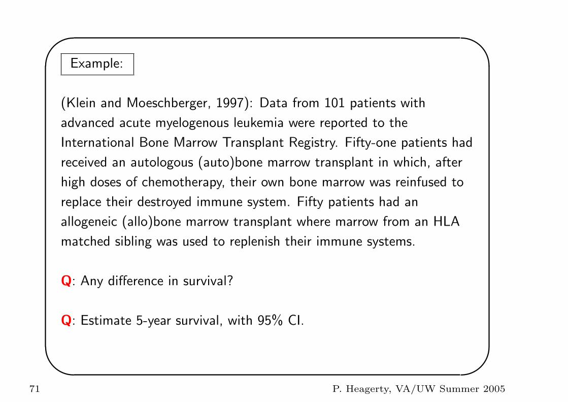
(Klein and Moeschberger, 1997): Data from 101 patients with
advanced acute myelogenous leukemia were reported to the
International Bone Marrow Transplant Registry. Fifty-one patients had
received an autologous (auto)bone marrow transplant in which, after
high doses of chemotherapy, their own bone marrow was reinfused to
replace their destroyed immune system. Fifty patients had an
allogeneic (allo)bone marrow transplant where marrow from an HLA
matched sibling was used to replenish their immune systems.
Q: Any difference in survival?
Q: Estimate 5-year survival, with 95% CI.
71 P. Heagerty, VA/UW Summer 2005
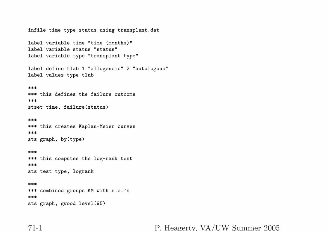
infile time type status using transplant.dat
label variable time "time (months)"label variable status "status"label variable type "transplant type"
label define tlab 1 "allogeneic" 2 "autologous"label values type tlab
****** this defines the failure outcome***stset time, failure(status)
****** this creates Kaplan-Meier curves***sts graph, by(type)
****** this computes the log-rank test***sts test type, logrank
****** combined groups KM with s.e.’s***sts graph, gwood level(95)
71-1 P. Heagerty, VA/UW Summer 2005
****** show the S(t) and s.e.’s***sts liststs list, by(type)
71-2 P. Heagerty, VA/UW Summer 2005
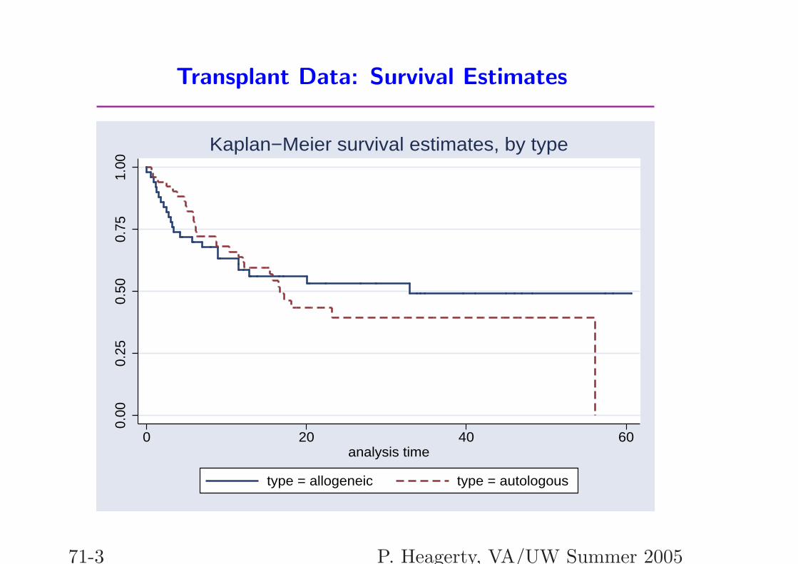
Transplant Data: Survival Estimates
0.00
0.25
0.50
0.75
1.00
0 20 40 60analysis time
type = allogeneic type = autologous
Kaplan−Meier survival estimates, by type
71-3 P. Heagerty, VA/UW Summer 2005
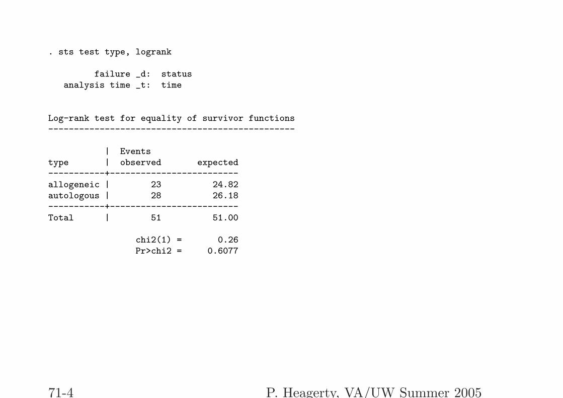
. sts test type, logrank
failure _d: statusanalysis time _t: time
Log-rank test for equality of survivor functions------------------------------------------------
| Eventstype | observed expected-----------+-------------------------allogeneic | 23 24.82autologous | 28 26.18-----------+-------------------------Total | 51 51.00
chi2(1) = 0.26Pr>chi2 = 0.6077
71-4 P. Heagerty, VA/UW Summer 2005
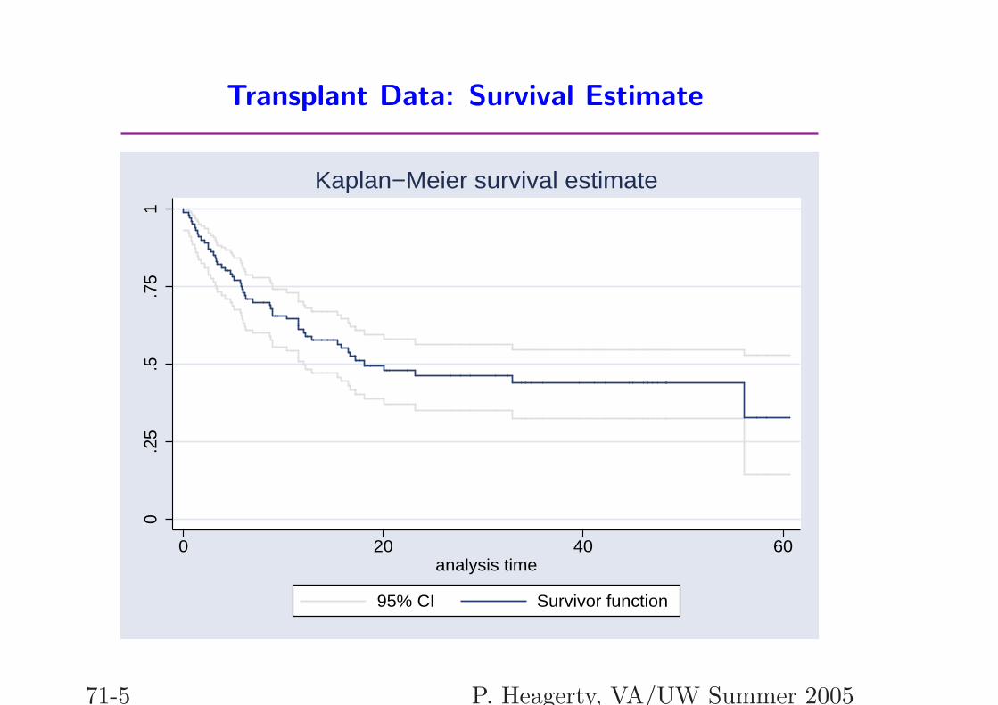
Transplant Data: Survival Estimate
0.2
5.5
.75
1
0 20 40 60analysis time
95% CI Survivor function
Kaplan−Meier survival estimate
71-5 P. Heagerty, VA/UW Summer 2005
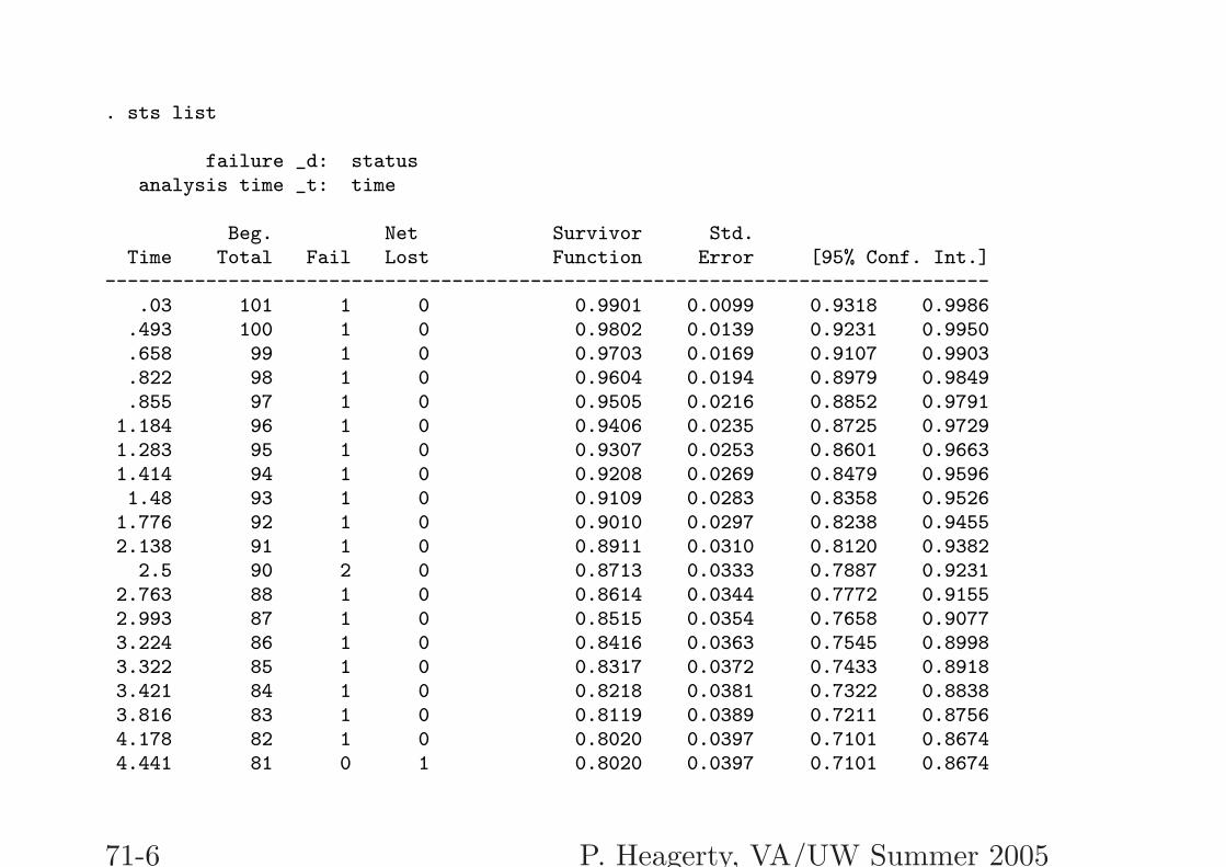
. sts list
failure _d: statusanalysis time _t: time
Beg. Net Survivor Std.Time Total Fail Lost Function Error [95% Conf. Int.]
-------------------------------------------------------------------------------.03 101 1 0 0.9901 0.0099 0.9318 0.9986.493 100 1 0 0.9802 0.0139 0.9231 0.9950.658 99 1 0 0.9703 0.0169 0.9107 0.9903.822 98 1 0 0.9604 0.0194 0.8979 0.9849.855 97 1 0 0.9505 0.0216 0.8852 0.9791
1.184 96 1 0 0.9406 0.0235 0.8725 0.97291.283 95 1 0 0.9307 0.0253 0.8601 0.96631.414 94 1 0 0.9208 0.0269 0.8479 0.95961.48 93 1 0 0.9109 0.0283 0.8358 0.9526
1.776 92 1 0 0.9010 0.0297 0.8238 0.94552.138 91 1 0 0.8911 0.0310 0.8120 0.9382
2.5 90 2 0 0.8713 0.0333 0.7887 0.92312.763 88 1 0 0.8614 0.0344 0.7772 0.91552.993 87 1 0 0.8515 0.0354 0.7658 0.90773.224 86 1 0 0.8416 0.0363 0.7545 0.89983.322 85 1 0 0.8317 0.0372 0.7433 0.89183.421 84 1 0 0.8218 0.0381 0.7322 0.88383.816 83 1 0 0.8119 0.0389 0.7211 0.87564.178 82 1 0 0.8020 0.0397 0.7101 0.86744.441 81 0 1 0.8020 0.0397 0.7101 0.8674
71-6 P. Heagerty, VA/UW Summer 2005
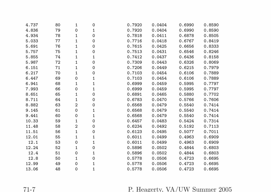
4.737 80 1 0 0.7920 0.0404 0.6990 0.85904.836 79 0 1 0.7920 0.0404 0.6990 0.85904.934 78 1 0 0.7818 0.0411 0.6878 0.85055.033 77 1 0 0.7716 0.0418 0.6767 0.84195.691 76 1 0 0.7615 0.0425 0.6656 0.83335.757 75 1 0 0.7513 0.0431 0.6546 0.82465.855 74 1 1 0.7412 0.0437 0.6436 0.81585.987 72 1 0 0.7309 0.0443 0.6326 0.80696.151 71 1 0 0.7206 0.0449 0.6215 0.79796.217 70 1 0 0.7103 0.0454 0.6106 0.78896.447 69 0 1 0.7103 0.0454 0.6106 0.78896.941 68 1 1 0.6999 0.0459 0.5995 0.77977.993 66 0 1 0.6999 0.0459 0.5995 0.77978.651 65 1 0 0.6891 0.0465 0.5880 0.77028.711 64 1 0 0.6783 0.0470 0.5766 0.76068.882 63 2 0 0.6568 0.0479 0.5540 0.74149.145 61 0 1 0.6568 0.0479 0.5540 0.74149.441 60 0 1 0.6568 0.0479 0.5540 0.741410.33 59 1 0 0.6457 0.0483 0.5424 0.731411.48 58 2 0 0.6234 0.0492 0.5192 0.711311.51 56 1 0 0.6123 0.0495 0.5077 0.701112.01 55 1 1 0.6011 0.0499 0.4963 0.690912.1 53 0 1 0.6011 0.0499 0.4963 0.6909
12.24 52 1 0 0.5896 0.0502 0.4844 0.680312.4 51 0 1 0.5896 0.0502 0.4844 0.680312.8 50 1 0 0.5778 0.0506 0.4723 0.6695
12.99 49 0 1 0.5778 0.0506 0.4723 0.669513.06 48 0 1 0.5778 0.0506 0.4723 0.6695
71-7 P. Heagerty, VA/UW Summer 2005
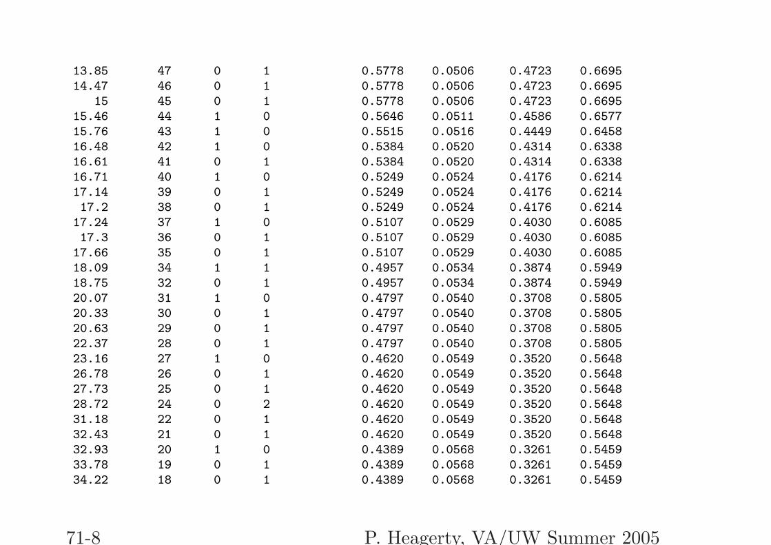
13.85 47 0 1 0.5778 0.0506 0.4723 0.669514.47 46 0 1 0.5778 0.0506 0.4723 0.6695
15 45 0 1 0.5778 0.0506 0.4723 0.669515.46 44 1 0 0.5646 0.0511 0.4586 0.657715.76 43 1 0 0.5515 0.0516 0.4449 0.645816.48 42 1 0 0.5384 0.0520 0.4314 0.633816.61 41 0 1 0.5384 0.0520 0.4314 0.633816.71 40 1 0 0.5249 0.0524 0.4176 0.621417.14 39 0 1 0.5249 0.0524 0.4176 0.621417.2 38 0 1 0.5249 0.0524 0.4176 0.6214
17.24 37 1 0 0.5107 0.0529 0.4030 0.608517.3 36 0 1 0.5107 0.0529 0.4030 0.6085
17.66 35 0 1 0.5107 0.0529 0.4030 0.608518.09 34 1 1 0.4957 0.0534 0.3874 0.594918.75 32 0 1 0.4957 0.0534 0.3874 0.594920.07 31 1 0 0.4797 0.0540 0.3708 0.580520.33 30 0 1 0.4797 0.0540 0.3708 0.580520.63 29 0 1 0.4797 0.0540 0.3708 0.580522.37 28 0 1 0.4797 0.0540 0.3708 0.580523.16 27 1 0 0.4620 0.0549 0.3520 0.564826.78 26 0 1 0.4620 0.0549 0.3520 0.564827.73 25 0 1 0.4620 0.0549 0.3520 0.564828.72 24 0 2 0.4620 0.0549 0.3520 0.564831.18 22 0 1 0.4620 0.0549 0.3520 0.564832.43 21 0 1 0.4620 0.0549 0.3520 0.564832.93 20 1 0 0.4389 0.0568 0.3261 0.545933.78 19 0 1 0.4389 0.0568 0.3261 0.545934.22 18 0 1 0.4389 0.0568 0.3261 0.5459
71-8 P. Heagerty, VA/UW Summer 2005
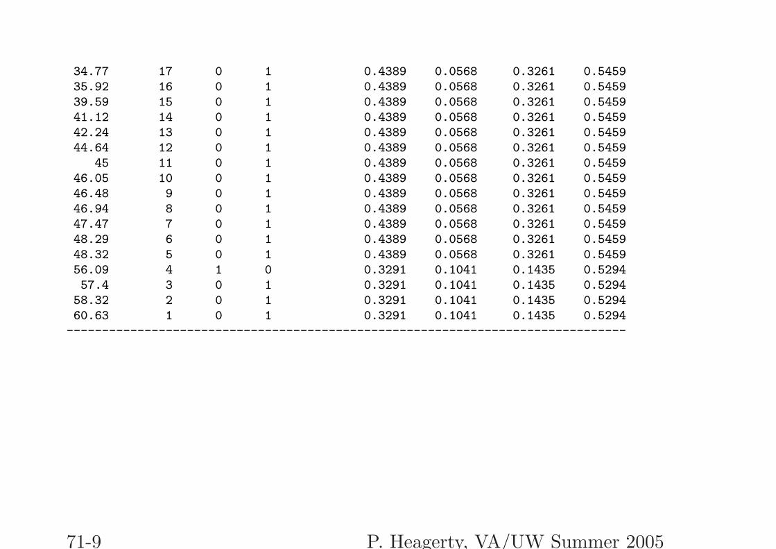
34.77 17 0 1 0.4389 0.0568 0.3261 0.545935.92 16 0 1 0.4389 0.0568 0.3261 0.545939.59 15 0 1 0.4389 0.0568 0.3261 0.545941.12 14 0 1 0.4389 0.0568 0.3261 0.545942.24 13 0 1 0.4389 0.0568 0.3261 0.545944.64 12 0 1 0.4389 0.0568 0.3261 0.5459
45 11 0 1 0.4389 0.0568 0.3261 0.545946.05 10 0 1 0.4389 0.0568 0.3261 0.545946.48 9 0 1 0.4389 0.0568 0.3261 0.545946.94 8 0 1 0.4389 0.0568 0.3261 0.545947.47 7 0 1 0.4389 0.0568 0.3261 0.545948.29 6 0 1 0.4389 0.0568 0.3261 0.545948.32 5 0 1 0.4389 0.0568 0.3261 0.545956.09 4 1 0 0.3291 0.1041 0.1435 0.529457.4 3 0 1 0.3291 0.1041 0.1435 0.5294
58.32 2 0 1 0.3291 0.1041 0.1435 0.529460.63 1 0 1 0.3291 0.1041 0.1435 0.5294-------------------------------------------------------------------------------
71-9 P. Heagerty, VA/UW Summer 2005
'
&
$
%
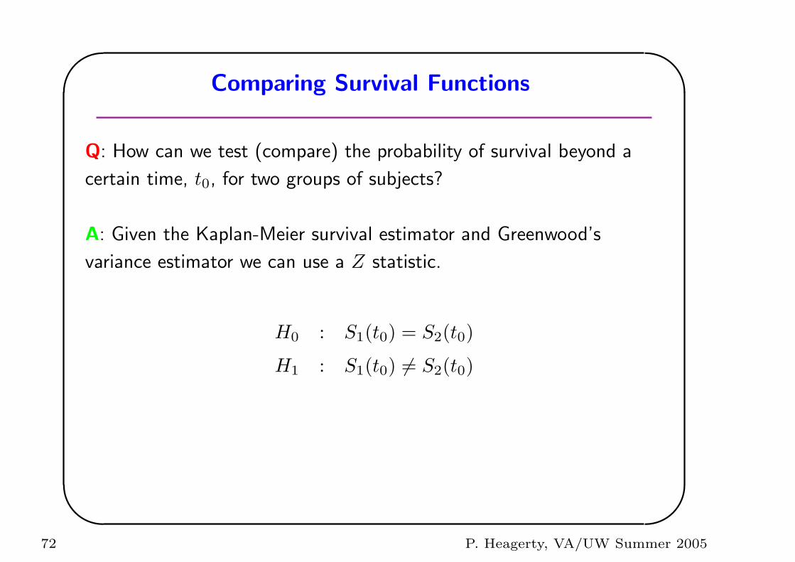
Comparing Survival Functions
Q: How can we test (compare) the probability of survival beyond a
certain time, t0, for two groups of subjects?
A: Given the Kaplan-Meier survival estimator and Greenwood’s
variance estimator we can use a Z statistic.
H0 : S1(t0) = S2(t0)
H1 : S1(t0) 6= S2(t0)
72 P. Heagerty, VA/UW Summer 2005

'
&
$
%
Comparing Survival Functions
Z =S1(t0)− S2(t0)√
V [S1(t0)] + V [S2(t0)]
Z ∼ N(0, 1) under H0
73 P. Heagerty, VA/UW Summer 2005
'
&
$
%
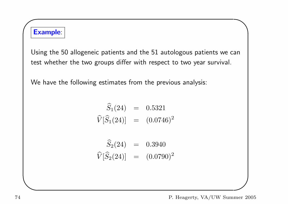
Example:
Using the 50 allogeneic patients and the 51 autologous patients we can
test whether the two groups differ with respect to two year survival.
We have the following estimates from the previous analysis:
S1(24) = 0.5321
V [S1(24)] = (0.0746)2
S2(24) = 0.3940
V [S2(24)] = (0.0790)2
74 P. Heagerty, VA/UW Summer 2005
'
&
$
%
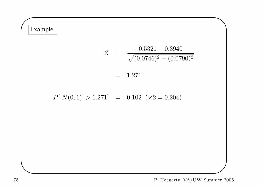
Example:
Z =0.5321− 0.3940√
(0.0746)2 + (0.0790)2
= 1.271
P [ N(0, 1) > 1.271] = 0.102 (×2 = 0.204)
75 P. Heagerty, VA/UW Summer 2005
'
&
$
%
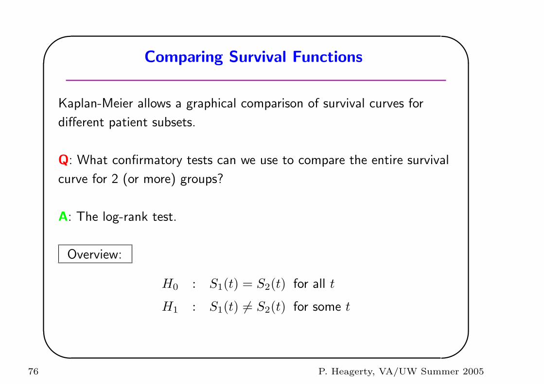
Comparing Survival Functions
Kaplan-Meier allows a graphical comparison of survival curves for
different patient subsets.
Q: What confirmatory tests can we use to compare the entire survival
curve for 2 (or more) groups?
A: The log-rank test.
Overview:
H0 : S1(t) = S2(t) for all t
H1 : S1(t) 6= S2(t) for some t
76 P. Heagerty, VA/UW Summer 2005
'
&
$
%
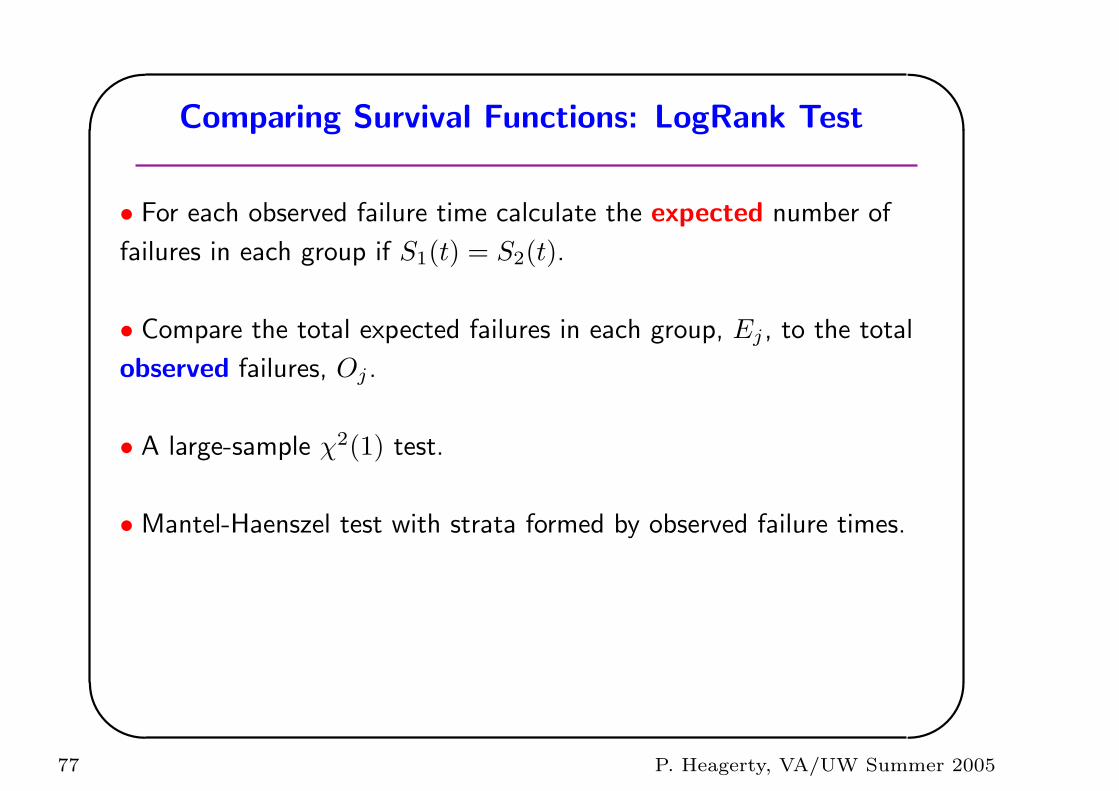
Comparing Survival Functions: LogRank Test
• For each observed failure time calculate the expected number of
failures in each group if S1(t) = S2(t).
• Compare the total expected failures in each group, Ej , to the total
observed failures, Oj .
• A large-sample χ2(1) test.
• Mantel-Haenszel test with strata formed by observed failure times.
77 P. Heagerty, VA/UW Summer 2005
'
&
$
%
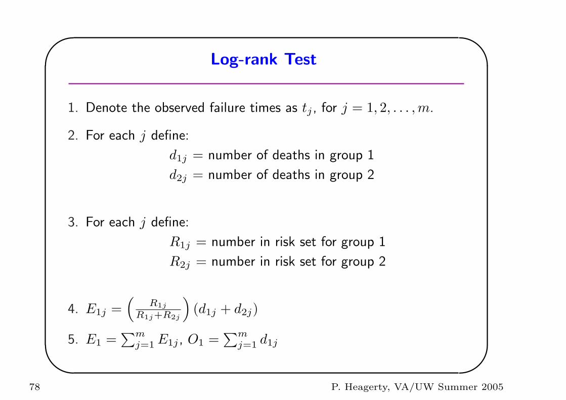
Log-rank Test
1. Denote the observed failure times as tj , for j = 1, 2, . . . , m.
2. For each j define:
d1j = number of deaths in group 1
d2j = number of deaths in group 2
3. For each j define:
R1j = number in risk set for group 1
R2j = number in risk set for group 2
4. E1j =(
R1j
R1j+R2j
)(d1j + d2j)
5. E1 =∑m
j=1 E1j , O1 =∑m
j=1 d1j
78 P. Heagerty, VA/UW Summer 2005
'
&
$
%
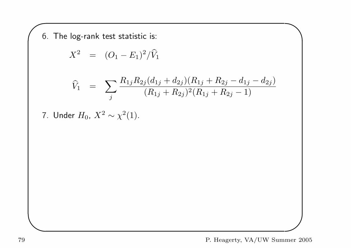
6. The log-rank test statistic is:
X2 = (O1 − E1)2/V1
V1 =∑
j
R1jR2j(d1j + d2j)(R1j + R2j − d1j − d2j)(R1j + R2j)2(R1j + R2j − 1)
7. Under H0, X2 ∼ χ2(1).
79 P. Heagerty, VA/UW Summer 2005
'
&
$
%
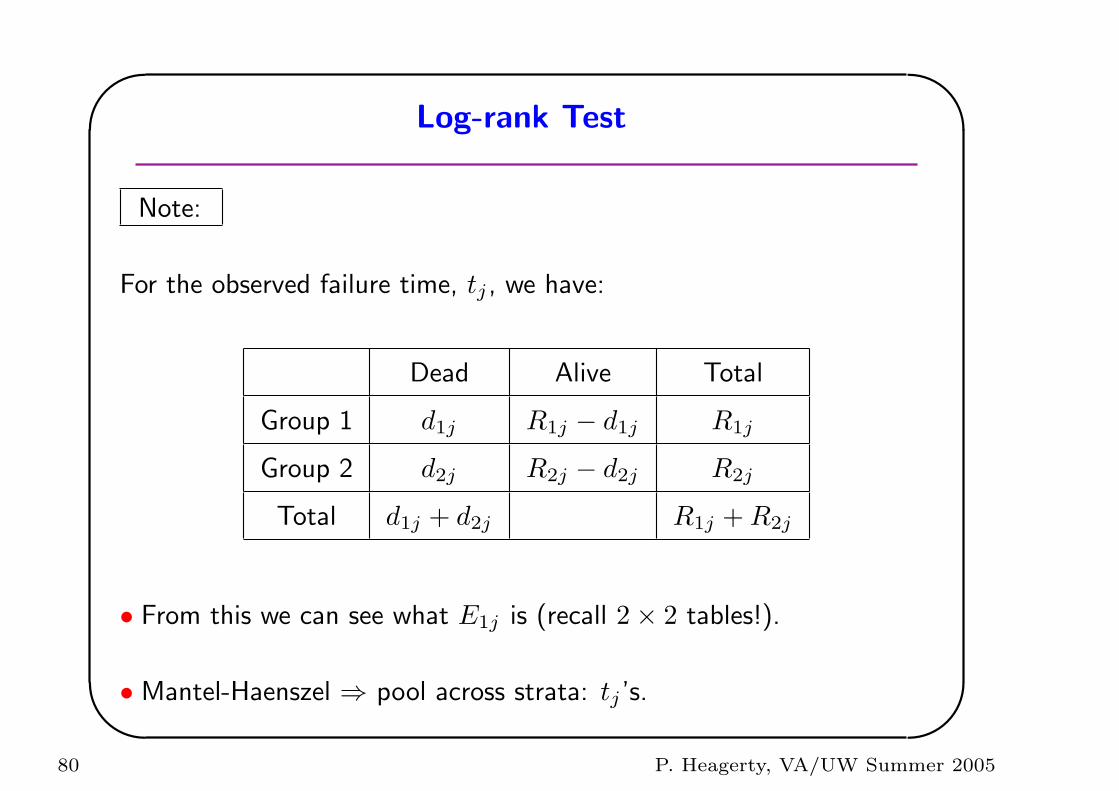
Log-rank Test
Note:
For the observed failure time, tj , we have:
Dead Alive Total
Group 1 d1j R1j − d1j R1j
Group 2 d2j R2j − d2j R2j
Total d1j + d2j R1j + R2j
• From this we can see what E1j is (recall 2× 2 tables!).
• Mantel-Haenszel ⇒ pool across strata: tj ’s.
80 P. Heagerty, VA/UW Summer 2005
'
&
$
%
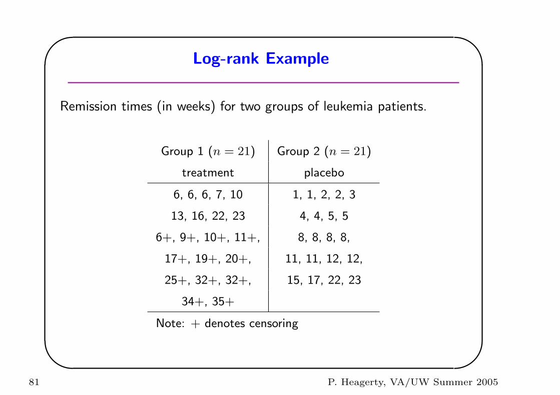
Log-rank Example
Remission times (in weeks) for two groups of leukemia patients.
Group 1 (n = 21) Group 2 (n = 21)
treatment placebo
6, 6, 6, 7, 10 1, 1, 2, 2, 3
13, 16, 22, 23 4, 4, 5, 5
6+, 9+, 10+, 11+, 8, 8, 8, 8,
17+, 19+, 20+, 11, 11, 12, 12,
25+, 32+, 32+, 15, 17, 22, 23
34+, 35+
Note: + denotes censoring
81 P. Heagerty, VA/UW Summer 2005
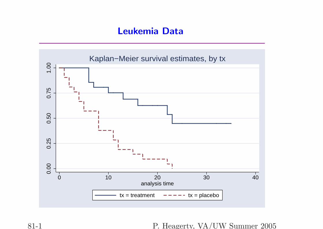
Leukemia Data
0.00
0.25
0.50
0.75
1.00
0 10 20 30 40analysis time
tx = treatment tx = placebo
Kaplan−Meier survival estimates, by tx
81-1 P. Heagerty, VA/UW Summer 2005
'
&
$
%
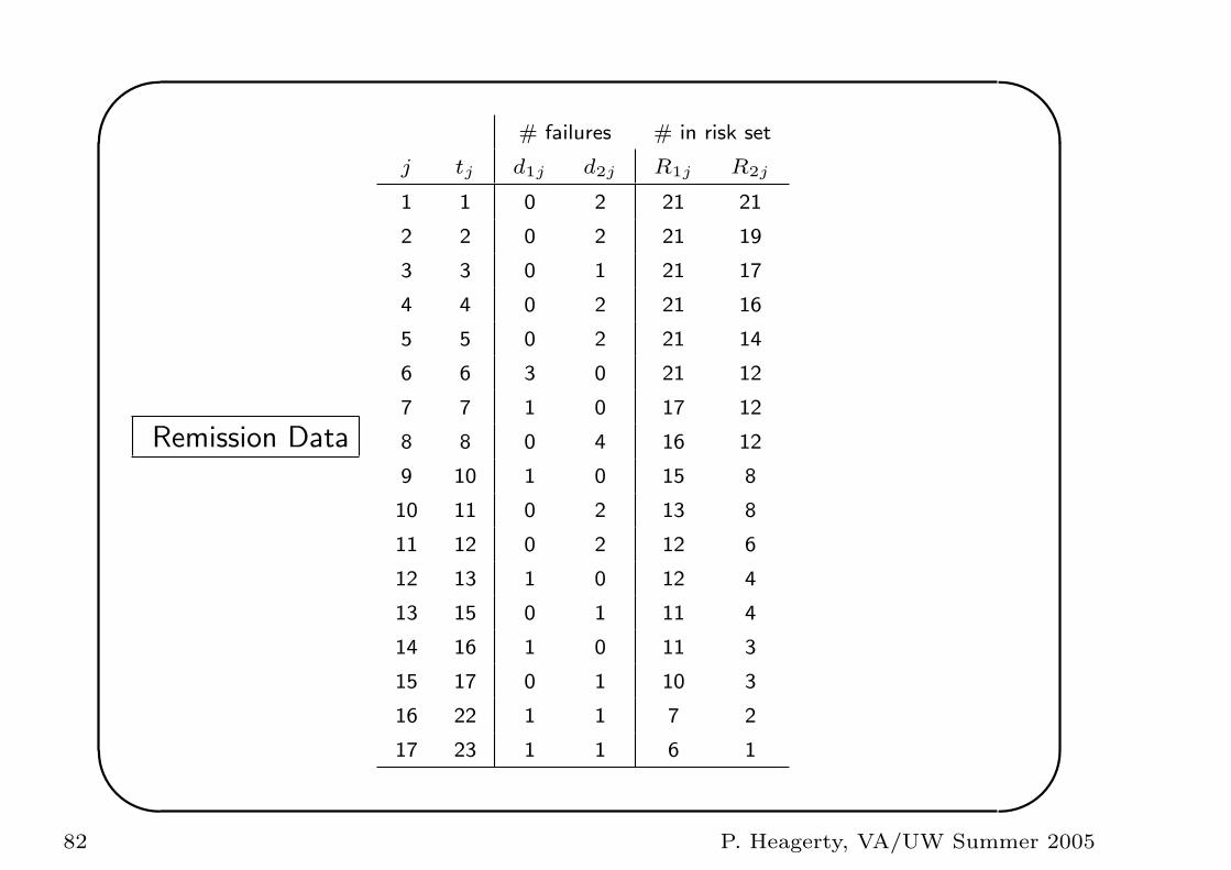
Remission Data
# failures # in risk set
j tj d1j d2j R1j R2j
1 1 0 2 21 21
2 2 0 2 21 19
3 3 0 1 21 17
4 4 0 2 21 16
5 5 0 2 21 14
6 6 3 0 21 12
7 7 1 0 17 12
8 8 0 4 16 12
9 10 1 0 15 8
10 11 0 2 13 8
11 12 0 2 12 6
12 13 1 0 12 4
13 15 0 1 11 4
14 16 1 0 11 3
15 17 0 1 10 3
16 22 1 1 7 2
17 23 1 1 6 1
82 P. Heagerty, VA/UW Summer 2005
'
&
$
%
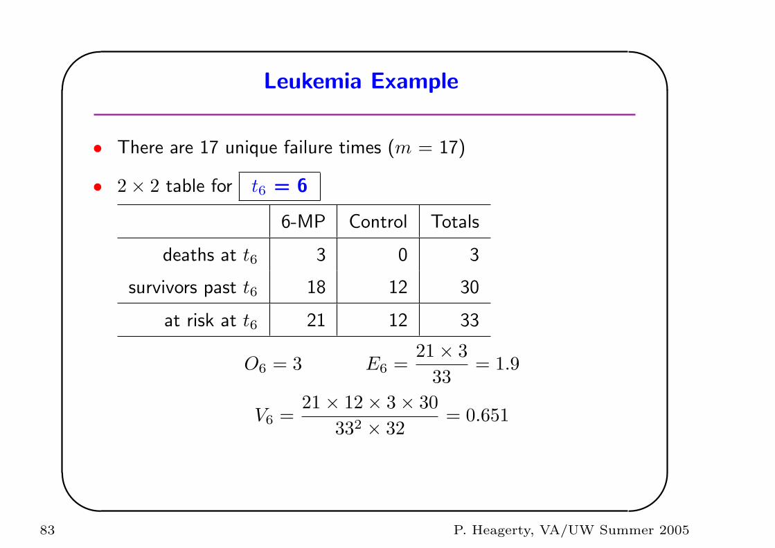
Leukemia Example
• There are 17 unique failure times (m = 17)
• 2× 2 table for t6 = 6
6-MP Control Totals
deaths at t6 3 0 3
survivors past t6 18 12 30
at risk at t6 21 12 33
O6 = 3 E6 =21× 3
33= 1.9
V6 =21× 12× 3× 30
332 × 32= 0.651
83 P. Heagerty, VA/UW Summer 2005
'
&
$
%
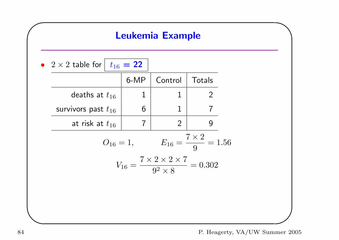
Leukemia Example
• 2× 2 table for t16 = 22
6-MP Control Totals
deaths at t16 1 1 2
survivors past t16 6 1 7
at risk at t16 7 2 9
O16 = 1, E16 =7× 2
9= 1.56
V16 =7× 2× 2× 7
92 × 8= 0.302
84 P. Heagerty, VA/UW Summer 2005
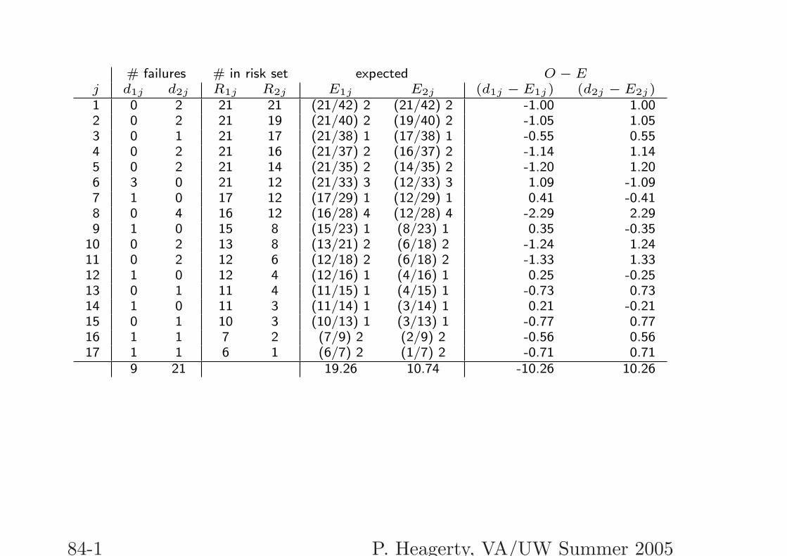
# failures # in risk set expected O − Ej d1j d2j R1j R2j E1j E2j (d1j − E1j) (d2j − E2j)1 0 2 21 21 (21/42) 2 (21/42) 2 -1.00 1.002 0 2 21 19 (21/40) 2 (19/40) 2 -1.05 1.053 0 1 21 17 (21/38) 1 (17/38) 1 -0.55 0.554 0 2 21 16 (21/37) 2 (16/37) 2 -1.14 1.145 0 2 21 14 (21/35) 2 (14/35) 2 -1.20 1.206 3 0 21 12 (21/33) 3 (12/33) 3 1.09 -1.097 1 0 17 12 (17/29) 1 (12/29) 1 0.41 -0.418 0 4 16 12 (16/28) 4 (12/28) 4 -2.29 2.299 1 0 15 8 (15/23) 1 (8/23) 1 0.35 -0.35
10 0 2 13 8 (13/21) 2 (6/18) 2 -1.24 1.2411 0 2 12 6 (12/18) 2 (6/18) 2 -1.33 1.3312 1 0 12 4 (12/16) 1 (4/16) 1 0.25 -0.2513 0 1 11 4 (11/15) 1 (4/15) 1 -0.73 0.7314 1 0 11 3 (11/14) 1 (3/14) 1 0.21 -0.2115 0 1 10 3 (10/13) 1 (3/13) 1 -0.77 0.7716 1 1 7 2 (7/9) 2 (2/9) 2 -0.56 0.5617 1 1 6 1 (6/7) 2 (1/7) 2 -0.71 0.71
9 21 19.26 10.74 -10.26 10.26
84-1 P. Heagerty, VA/UW Summer 2005
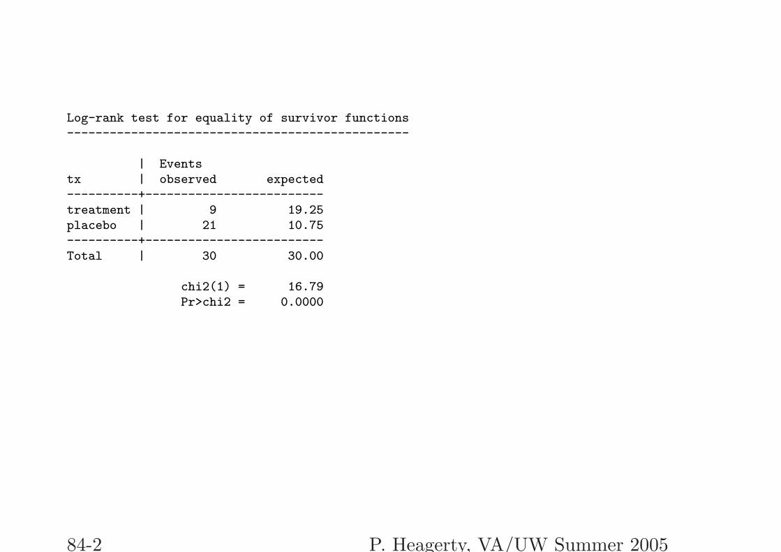
Log-rank test for equality of survivor functions------------------------------------------------
| Eventstx | observed expected----------+-------------------------treatment | 9 19.25placebo | 21 10.75----------+-------------------------Total | 30 30.00
chi2(1) = 16.79Pr>chi2 = 0.0000
84-2 P. Heagerty, VA/UW Summer 2005
'
&
$
%
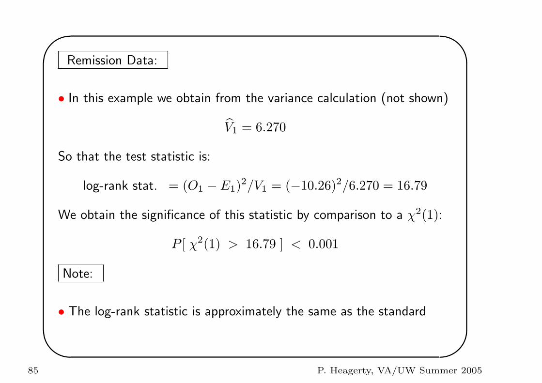
Remission Data:
• In this example we obtain from the variance calculation (not shown)
V1 = 6.270
So that the test statistic is:
log-rank stat. = (O1 − E1)2/V1 = (−10.26)2/6.270 = 16.79
We obtain the significance of this statistic by comparison to a χ2(1):
P [ χ2(1) > 16.79 ] < 0.001
Note:
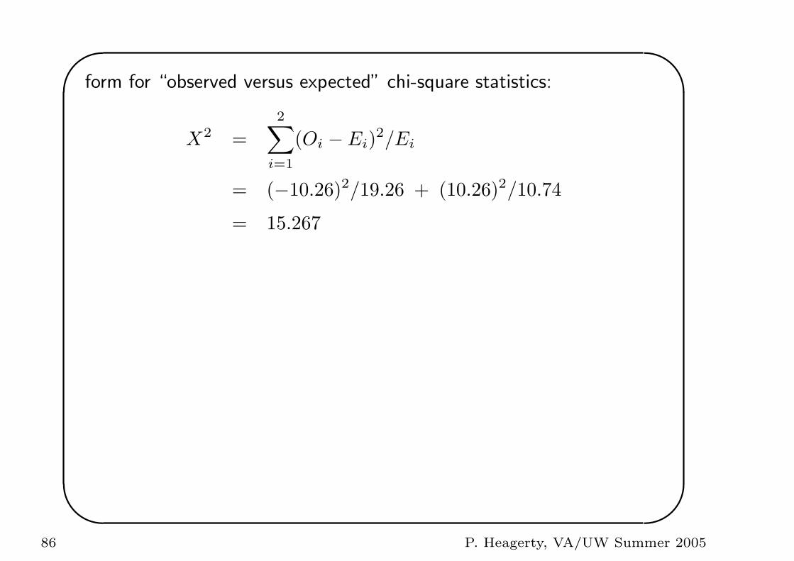
• The log-rank statistic is approximately the same as the standard
85 P. Heagerty, VA/UW Summer 2005
'
&
$
%
form for “observed versus expected” chi-square statistics:
X2 =2∑
i=1
(Oi − Ei)2/Ei
= (−10.26)2/19.26 + (10.26)2/10.74
= 15.267
86 P. Heagerty, VA/UW Summer 2005
'
&
$
%
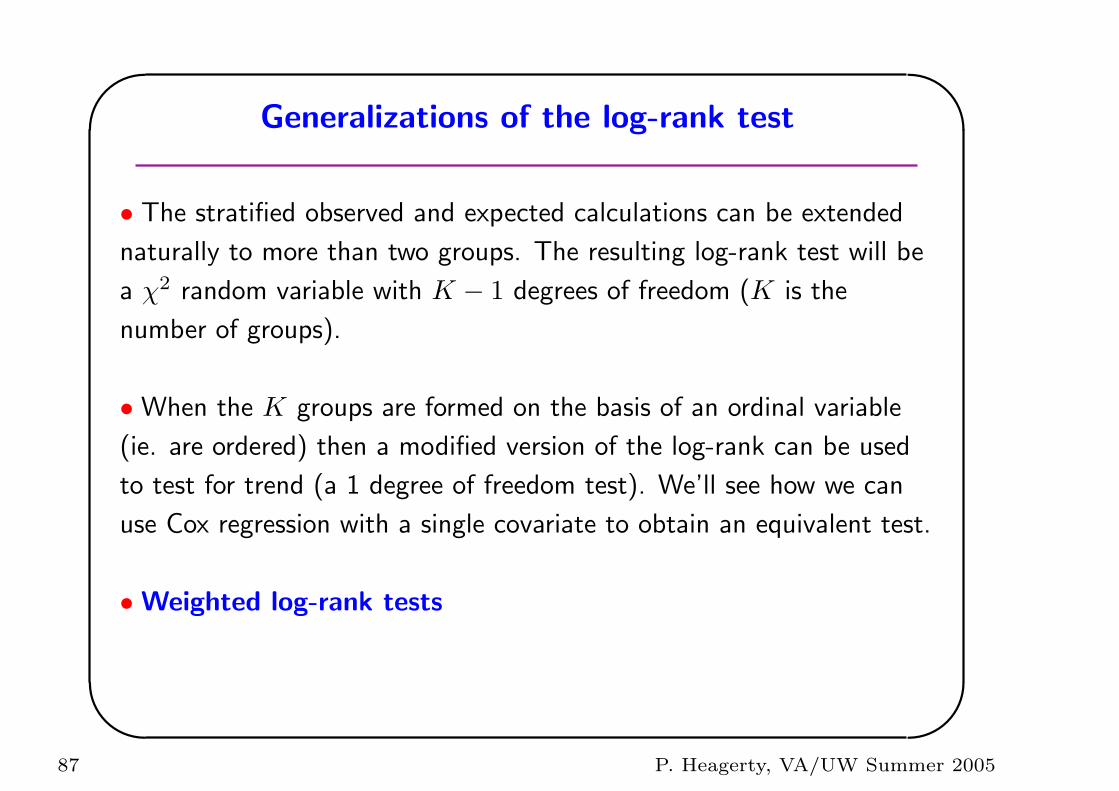
Generalizations of the log-rank test
• The stratified observed and expected calculations can be extended
naturally to more than two groups. The resulting log-rank test will be
a χ2 random variable with K − 1 degrees of freedom (K is the
number of groups).
• When the K groups are formed on the basis of an ordinal variable
(ie. are ordered) then a modified version of the log-rank can be used
to test for trend (a 1 degree of freedom test). We’ll see how we can
use Cox regression with a single covariate to obtain an equivalent test.
• Weighted log-rank tests
87 P. Heagerty, VA/UW Summer 2005
'
&
$
%
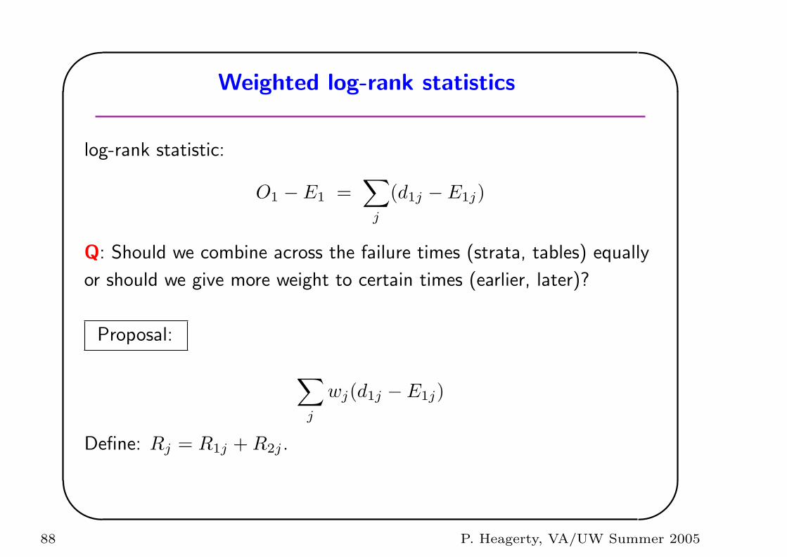
Weighted log-rank statistics
log-rank statistic:
O1 − E1 =∑
j
(d1j − E1j)
Q: Should we combine across the failure times (strata, tables) equally
or should we give more weight to certain times (earlier, later)?
Proposal:
∑
j
wj(d1j − E1j)
Define: Rj = R1j + R2j .
88 P. Heagerty, VA/UW Summer 2005
'
&
$
%
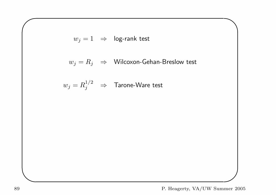
wj = 1 ⇒ log-rank test
wj = Rj ⇒ Wilcoxon-Gehan-Breslow test
wj = R1/2j ⇒ Tarone-Ware test
89 P. Heagerty, VA/UW Summer 2005
'
&
$
%
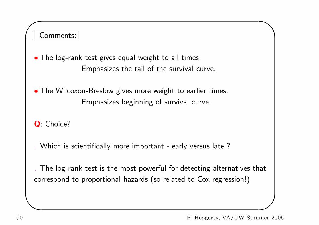
Comments:
• The log-rank test gives equal weight to all times.
Emphasizes the tail of the survival curve.
• The Wilcoxon-Breslow gives more weight to earlier times.
Emphasizes beginning of survival curve.
Q: Choice?
. Which is scientifically more important - early versus late ?
. The log-rank test is the most powerful for detecting alternatives that
correspond to proportional hazards (so related to Cox regression!)
90 P. Heagerty, VA/UW Summer 2005
'
&
$
%
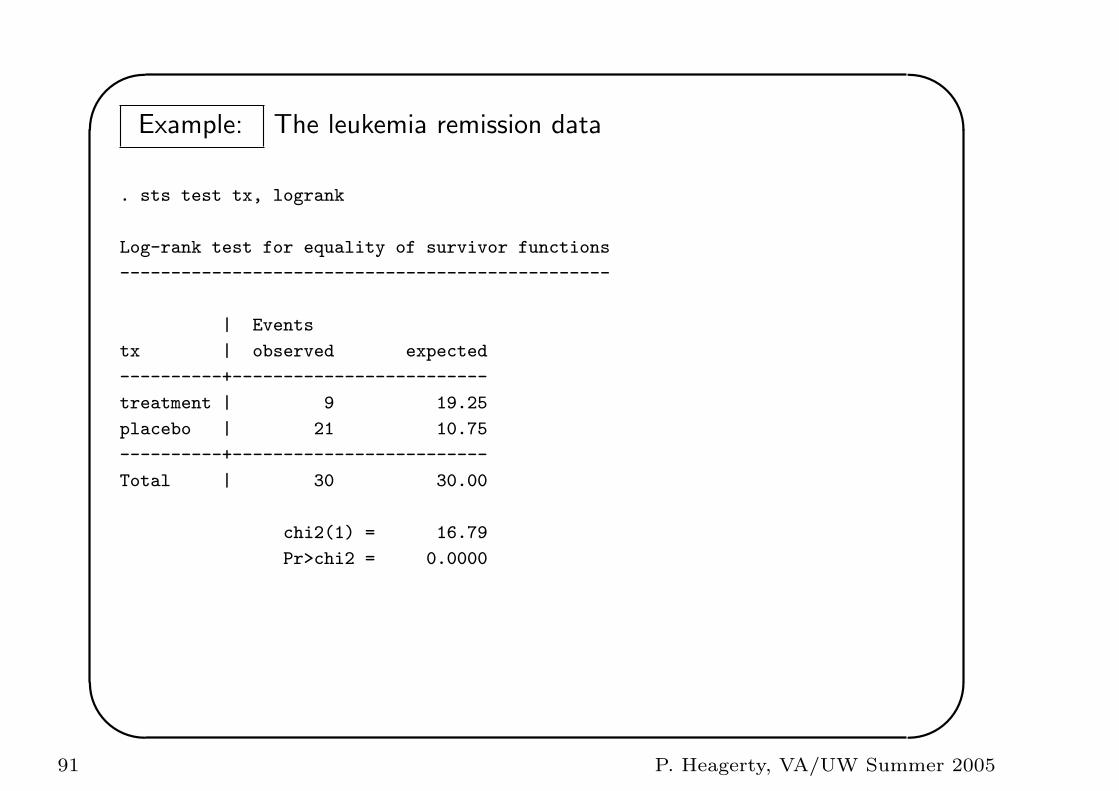
Example: The leukemia remission data
. sts test tx, logrank
Log-rank test for equality of survivor functions
------------------------------------------------
| Events
tx | observed expected
----------+-------------------------
treatment | 9 19.25
placebo | 21 10.75
----------+-------------------------
Total | 30 30.00
chi2(1) = 16.79
Pr>chi2 = 0.0000
91 P. Heagerty, VA/UW Summer 2005
'
&
$
%
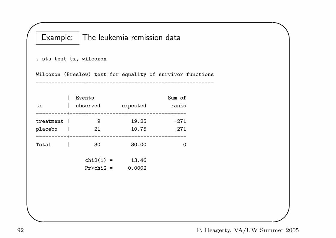
Example: The leukemia remission data
. sts test tx, wilcoxon
Wilcoxon (Breslow) test for equality of survivor functions
----------------------------------------------------------
| Events Sum of
tx | observed expected ranks
----------+--------------------------------------
treatment | 9 19.25 -271
placebo | 21 10.75 271
----------+--------------------------------------
Total | 30 30.00 0
chi2(1) = 13.46
Pr>chi2 = 0.0002
92 P. Heagerty, VA/UW Summer 2005
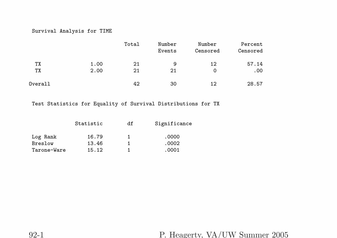
Survival Analysis for TIME
Total Number Number PercentEvents Censored Censored
TX 1.00 21 9 12 57.14TX 2.00 21 21 0 .00
Overall 42 30 12 28.57
Test Statistics for Equality of Survival Distributions for TX
Statistic df Significance
Log Rank 16.79 1 .0000Breslow 13.46 1 .0002Tarone-Ware 15.12 1 .0001
92-1 P. Heagerty, VA/UW Summer 2005
'
&
$
%
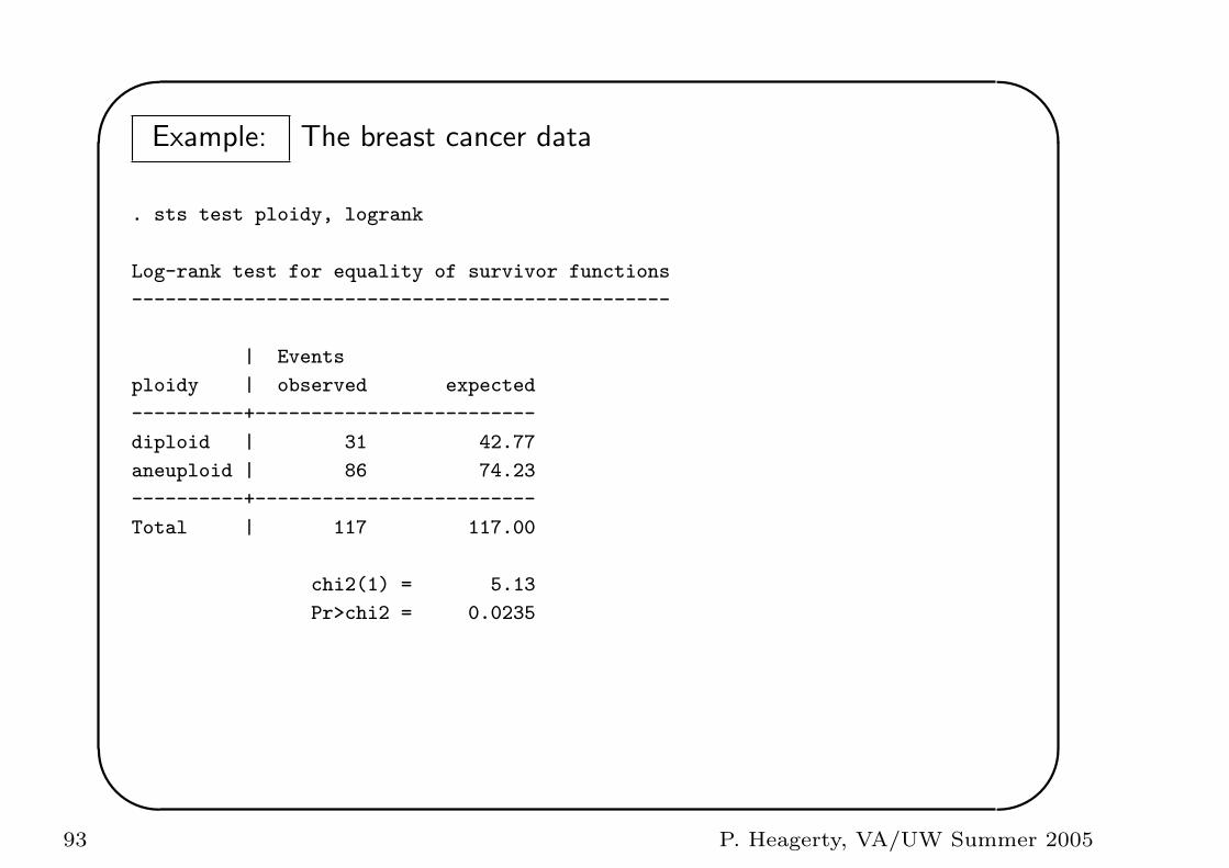
Example: The breast cancer data
. sts test ploidy, logrank
Log-rank test for equality of survivor functions
------------------------------------------------
| Events
ploidy | observed expected
----------+-------------------------
diploid | 31 42.77
aneuploid | 86 74.23
----------+-------------------------
Total | 117 117.00
chi2(1) = 5.13
Pr>chi2 = 0.0235
93 P. Heagerty, VA/UW Summer 2005
'
&
$
%
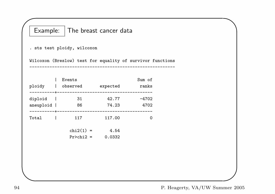
Example: The breast cancer data
. sts test ploidy, wilcoxon
Wilcoxon (Breslow) test for equality of survivor functions
----------------------------------------------------------
| Events Sum of
ploidy | observed expected ranks
----------+--------------------------------------
diploid | 31 42.77 -4702
aneuploid | 86 74.23 4702
----------+--------------------------------------
Total | 117 117.00 0
chi2(1) = 4.54
Pr>chi2 = 0.0332
94 P. Heagerty, VA/UW Summer 2005
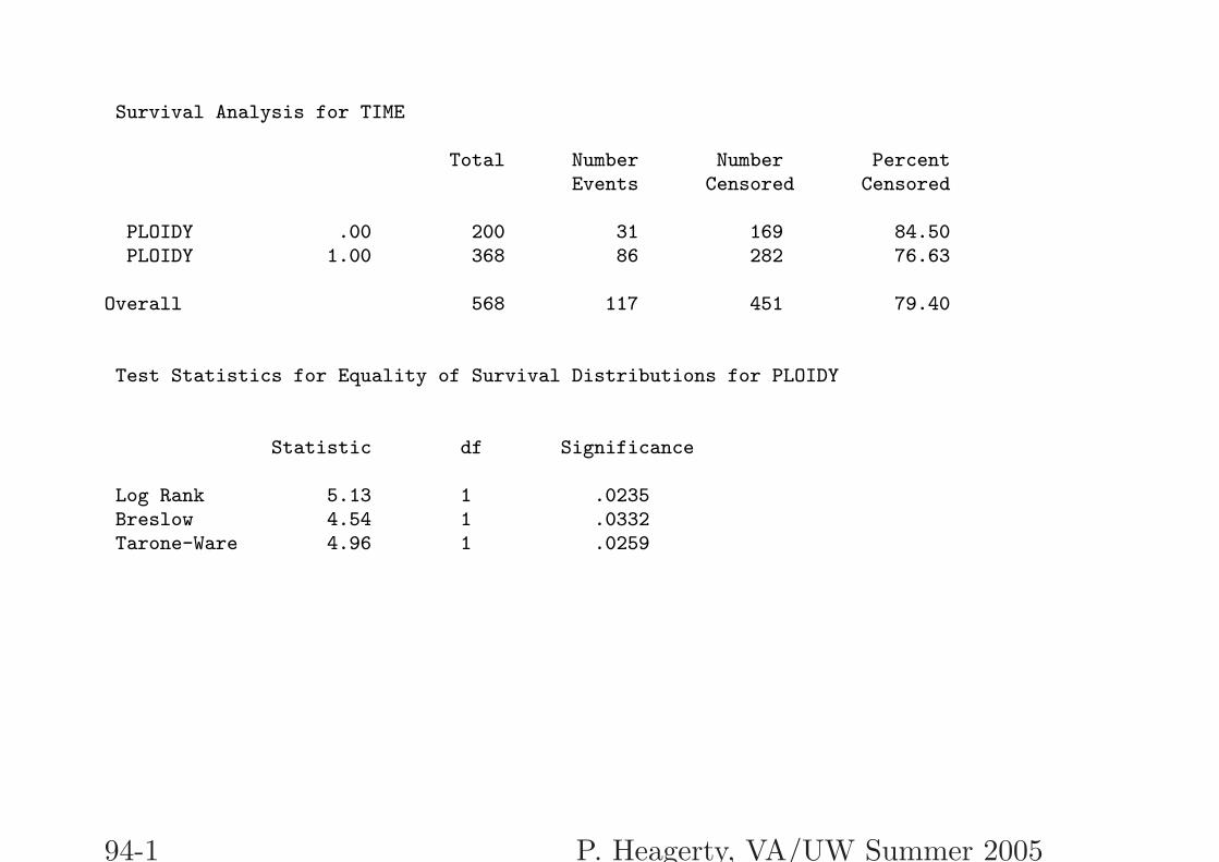
Survival Analysis for TIME
Total Number Number PercentEvents Censored Censored
PLOIDY .00 200 31 169 84.50PLOIDY 1.00 368 86 282 76.63
Overall 568 117 451 79.40
Test Statistics for Equality of Survival Distributions for PLOIDY
Statistic df Significance
Log Rank 5.13 1 .0235Breslow 4.54 1 .0332Tarone-Ware 4.96 1 .0259
94-1 P. Heagerty, VA/UW Summer 2005
'
&
$
%
Summary
1. We can compare survival probabilities at any single time, t0, with
a familiar 2-sample statistic.
2. We can compare the entire survival function for 2 groups using the
log-rank test.
3. The log-rank test can easily be extended to K groups (K ≥ 2).
4. Alternative tests have been proposed that allow different weight to
be given to earlier and later times.
95 P. Heagerty, VA/UW Summer 2005
'
&
$
%
Hazard functions and models
• Hazard function
. Definition
. Relationship to incidence
. Cumulative hazard
. Relationship to survival fnx
• Cox regression
. Proportional hazards assumption
. “semi-parametric” model
. Estimation and Inference
. Estimation of baseline survival fnx
96 P. Heagerty, VA/UW Summer 2005
'
&
$
%
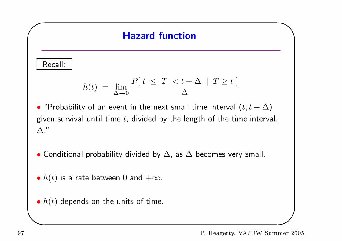
Hazard function
Recall:
h(t) = lim∆→0
P [ t ≤ T < t + ∆ | T ≥ t ]∆
• “Probability of an event in the next small time interval (t, t + ∆)
given survival until time t, divided by the length of the time interval,
∆.”
• Conditional probability divided by ∆, as ∆ becomes very small.
• h(t) is a rate between 0 and +∞.
• h(t) depends on the units of time.
97 P. Heagerty, VA/UW Summer 2005
'
&
$
%
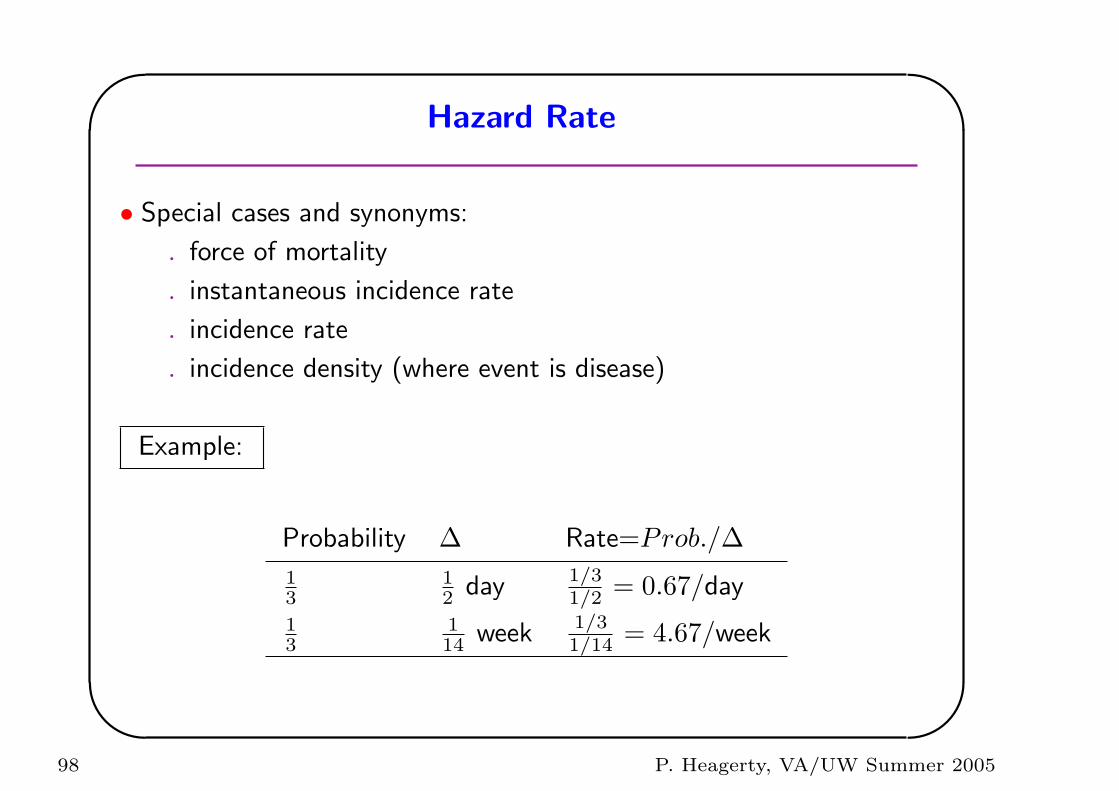
Hazard Rate
• Special cases and synonyms:
. force of mortality
. instantaneous incidence rate
. incidence rate
. incidence density (where event is disease)
Example:
Probability ∆ Rate=Prob./∆13
12 day 1/3
1/2 = 0.67/day
13
114 week 1/3
1/14 = 4.67/week
98 P. Heagerty, VA/UW Summer 2005
'
&
$
%
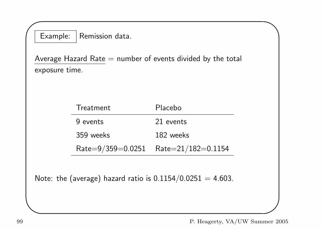
Example: Remission data.
Average Hazard Rate = number of events divided by the total
exposure time.
Treatment Placebo
9 events 21 events
359 weeks 182 weeks
Rate=9/359=0.0251 Rate=21/182=0.1154
Note: the (average) hazard ratio is 0.1154/0.0251 = 4.603.
99 P. Heagerty, VA/UW Summer 2005
'
&
$
%
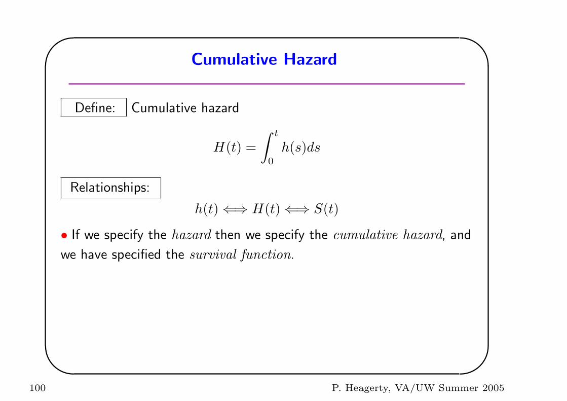
Cumulative Hazard
Define: Cumulative hazard
H(t) =∫ t
0
h(s)ds
Relationships:
h(t) ⇐⇒ H(t) ⇐⇒ S(t)
• If we specify the hazard then we specify the cumulative hazard, and
we have specified the survival function.
100 P. Heagerty, VA/UW Summer 2005
'
&
$
%
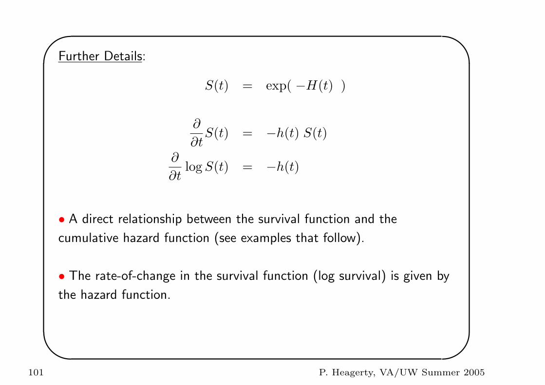
Further Details:
S(t) = exp( −H(t) )
∂
∂tS(t) = −h(t) S(t)
∂
∂tlog S(t) = −h(t)
• A direct relationship between the survival function and the
cumulative hazard function (see examples that follow).
• The rate-of-change in the survival function (log survival) is given by
the hazard function.
101 P. Heagerty, VA/UW Summer 2005
'
&
$
%
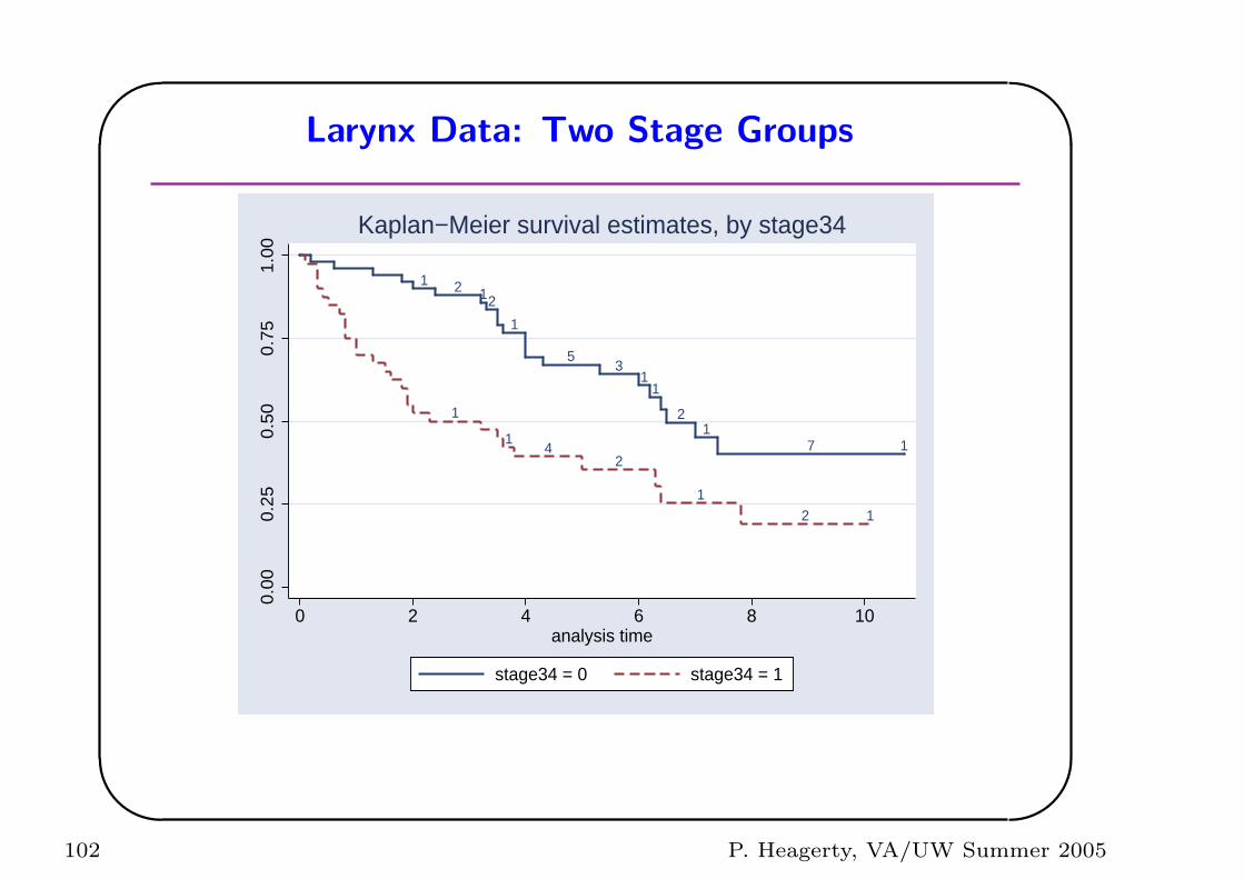
Larynx Data: Two Stage Groups
1
1
2 12
1
1
4
5
2
31
1
2
1
1
2
7
1
1
0.00
0.25
0.50
0.75
1.00
0 2 4 6 8 10analysis time
stage34 = 0 stage34 = 1
Kaplan−Meier survival estimates, by stage34
102 P. Heagerty, VA/UW Summer 2005
'
&
$
%
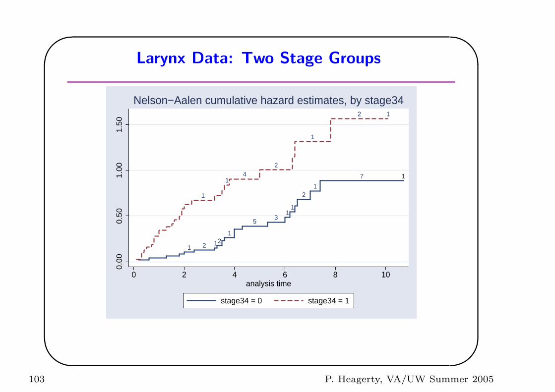
Larynx Data: Two Stage Groups
1
1
2 12
1
1
4
53
2
11
2
1
1
2
7
1
1
0.00
0.50
1.00
1.50
0 2 4 6 8 10analysis time
stage34 = 0 stage34 = 1
Nelson−Aalen cumulative hazard estimates, by stage34
103 P. Heagerty, VA/UW Summer 2005
'
&
$
%
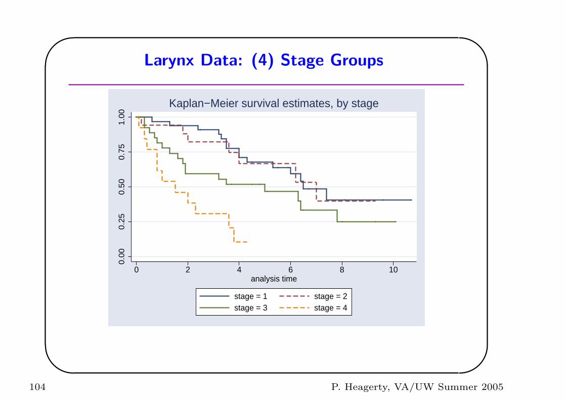
Larynx Data: (4) Stage Groups
0.00
0.25
0.50
0.75
1.00
0 2 4 6 8 10analysis time
stage = 1 stage = 2stage = 3 stage = 4
Kaplan−Meier survival estimates, by stage
104 P. Heagerty, VA/UW Summer 2005
'
&
$
%
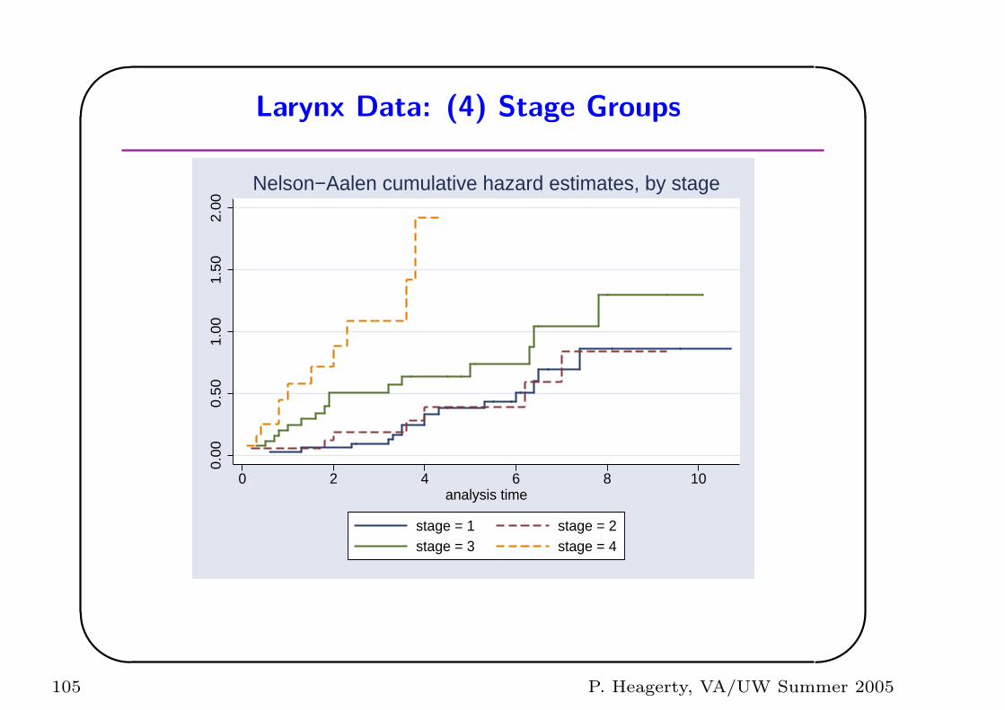
Larynx Data: (4) Stage Groups
0.00
0.50
1.00
1.50
2.00
0 2 4 6 8 10analysis time
stage = 1 stage = 2stage = 3 stage = 4
Nelson−Aalen cumulative hazard estimates, by stage
105 P. Heagerty, VA/UW Summer 2005
'
&
$
%
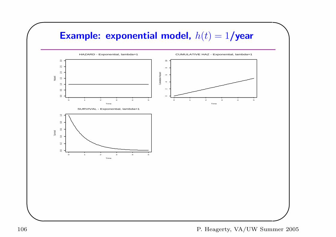
Example: exponential model, h(t) = 1/year
Time
Haza
rd
0 1 2 3 4 5
0.00.5
1.01.5
2.02.5
3.0
HAZARD - Exponential, lambda=1
Time
Cumu
lative
Haza
rd
0 1 2 3 4 5
02
46
810
CUMULATIVE HAZ - Exponential, lambda=1
Time
Survi
val
0 1 2 3 4 5
0.00.2
0.40.6
0.81.0
SURVIVAL - Exponential, lambda=1
106 P. Heagerty, VA/UW Summer 2005
'
&
$
%
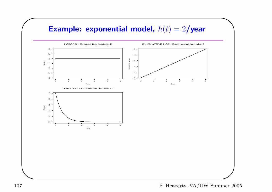
Example: exponential model, h(t) = 2/year
Time
Haza
rd
0 1 2 3 4 5
0.00.5
1.01.5
2.02.5
3.0
HAZARD - Exponential, lambda=2
Time
Cumu
lative
Haza
rd
0 1 2 3 4 5
02
46
810
CUMULATIVE HAZ - Exponential, lambda=2
Time
Survi
val
0 1 2 3 4 5
0.00.2
0.40.6
0.81.0
SURVIVAL - Exponential, lambda=2
107 P. Heagerty, VA/UW Summer 2005
'
&
$
%
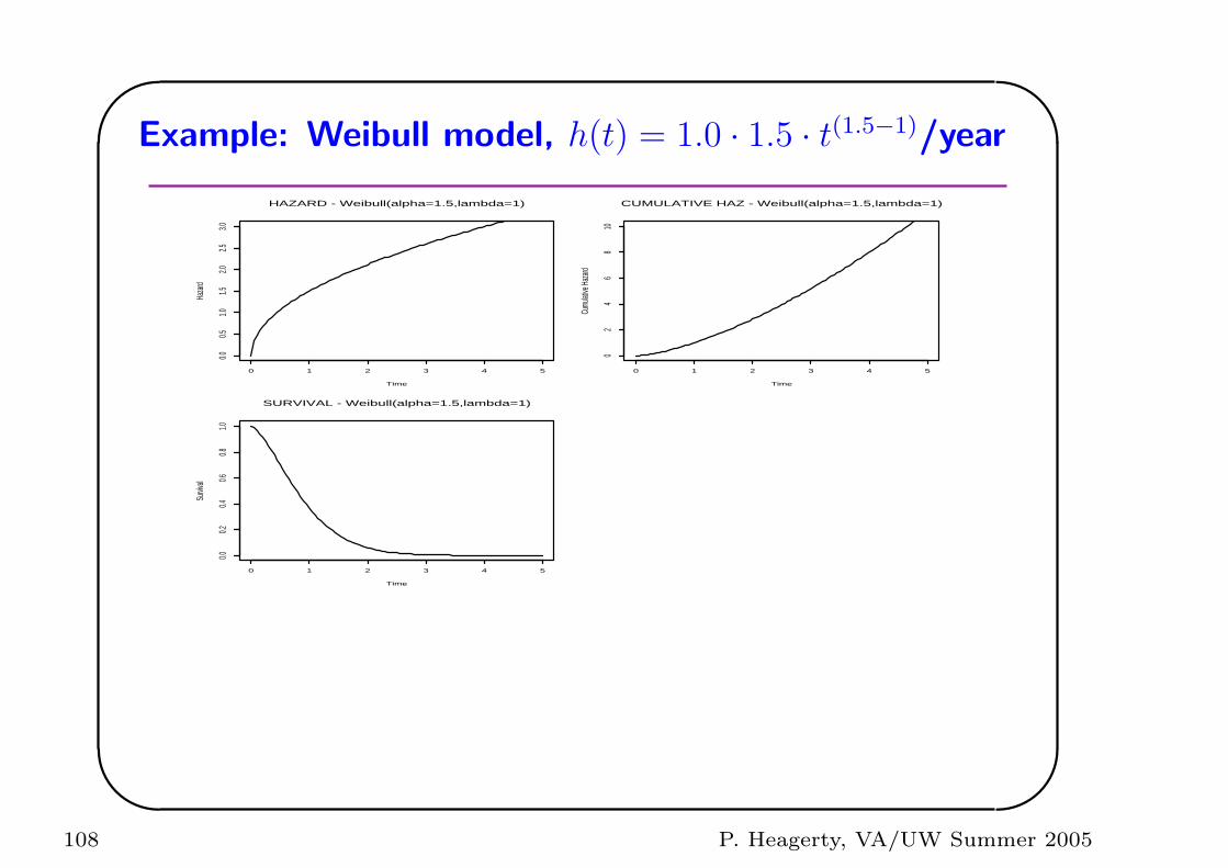
Example: Weibull model, h(t) = 1.0 · 1.5 · t(1.5−1)/year
Time
Haza
rd
0 1 2 3 4 5
0.00.5
1.01.5
2.02.5
3.0
HAZARD - Weibull(alpha=1.5,lambda=1)
Time
Cumu
lative
Haza
rd
0 1 2 3 4 5
02
46
810
CUMULATIVE HAZ - Weibull(alpha=1.5,lambda=1)
Time
Survi
val
0 1 2 3 4 5
0.00.2
0.40.6
0.81.0
SURVIVAL - Weibull(alpha=1.5,lambda=1)
108 P. Heagerty, VA/UW Summer 2005
'
&
$
%
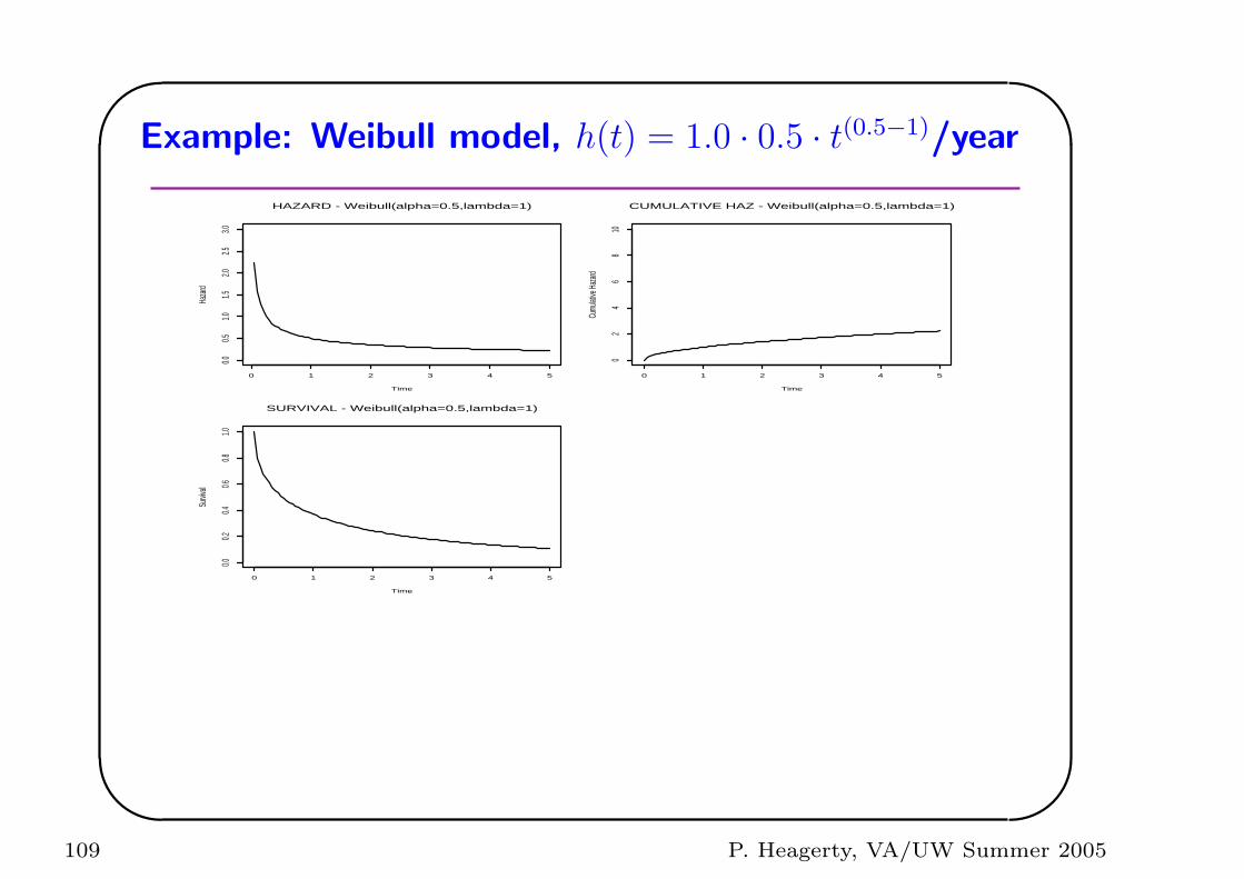
Example: Weibull model, h(t) = 1.0 · 0.5 · t(0.5−1)/year
Time
Haza
rd
0 1 2 3 4 5
0.00.5
1.01.5
2.02.5
3.0
HAZARD - Weibull(alpha=0.5,lambda=1)
Time
Cumu
lative
Haza
rd
0 1 2 3 4 5
02
46
810
CUMULATIVE HAZ - Weibull(alpha=0.5,lambda=1)
Time
Survi
val
0 1 2 3 4 5
0.00.2
0.40.6
0.81.0
SURVIVAL - Weibull(alpha=0.5,lambda=1)
109 P. Heagerty, VA/UW Summer 2005
'
&
$
%
Motivation
• We can use Kaplan-Meier to characterize survival when there are a
few large groups that we want to compare.
• With multiple covariates we can not stratify on all of the
predictors at once.
• It is reasonable to expect that many different factors influence
survival.
• How to use continuous covariates (without grouping)?.
110 P. Heagerty, VA/UW Summer 2005
'
&
$
%
Motivation
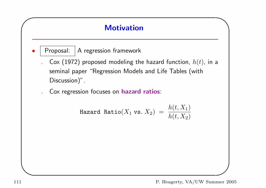
• Proposal: A regression framework
. Cox (1972) proposed modeling the hazard function, h(t), in a
seminal paper “Regression Models and Life Tables (with
Discussion)”.
. Cox regression focuses on hazard ratios:
Hazard Ratio(X1 vs. X2) =h(t,X1)h(t,X2)
111 P. Heagerty, VA/UW Summer 2005
'
&
$
%
Cox (1972)
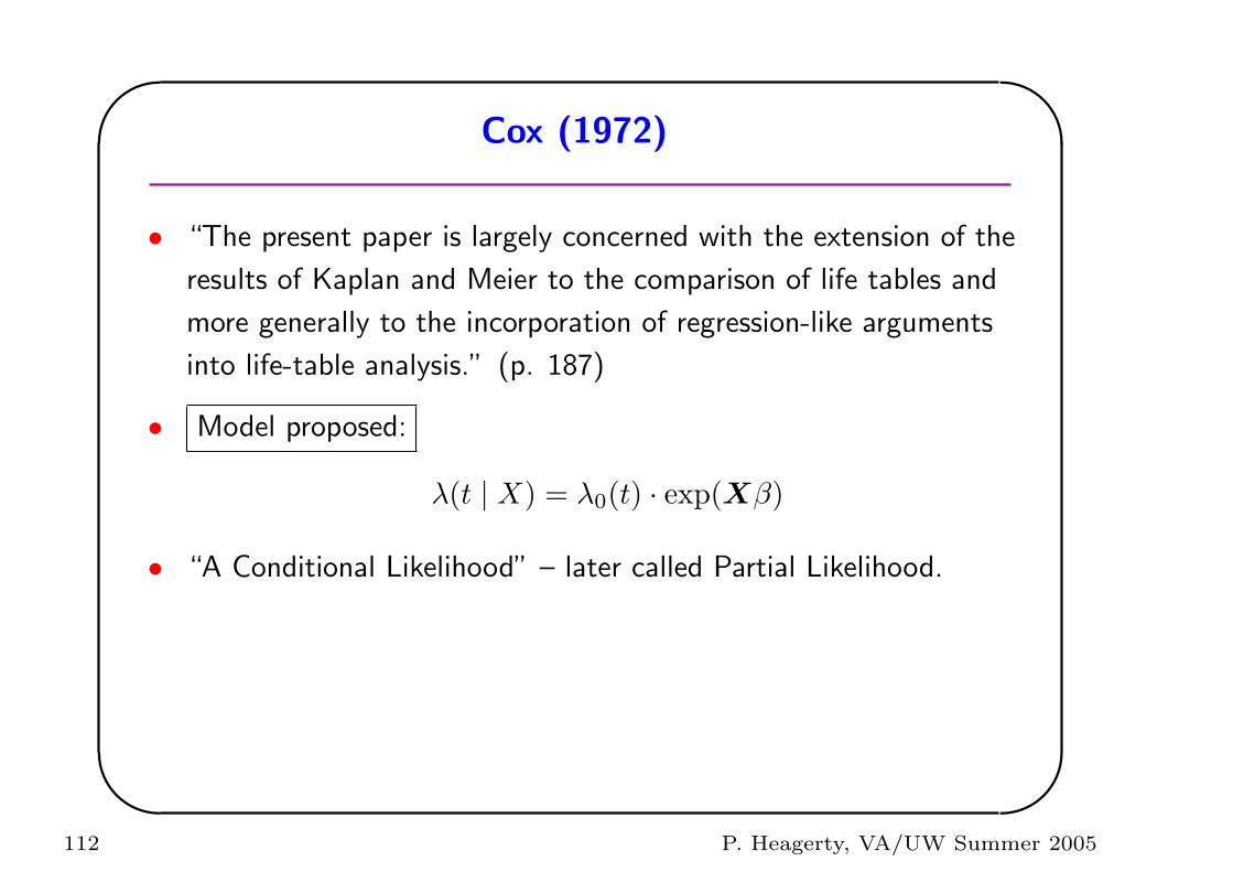
• “The present paper is largely concerned with the extension of the
results of Kaplan and Meier to the comparison of life tables and
more generally to the incorporation of regression-like arguments
into life-table analysis.” (p. 187)
• Model proposed:
λ(t | X) = λ0(t) · exp(Xβ)
• “A Conditional Likelihood” – later called Partial Likelihood.
112 P. Heagerty, VA/UW Summer 2005

'
&
$
%
Cox (1972)
• Discussion:
. “Mr. Richard Peto (Oxford University): I have greatly enjoyed
Professor Cox’s paper. It seems to me to formulate and to
solve the problem of regression of prognosis on other factors
perfectly, and it is very pretty.”
• Impact:
. Science Citation Index: 19,502 citations (17 Jan 2005)
. David R. Cox is knighted in 1985 in recognition of his scientific
contributions.
113 P. Heagerty, VA/UW Summer 2005
'
&
$
%
Sir David R. Cox
114 P. Heagerty, VA/UW Summer 2005
'
&
$
%
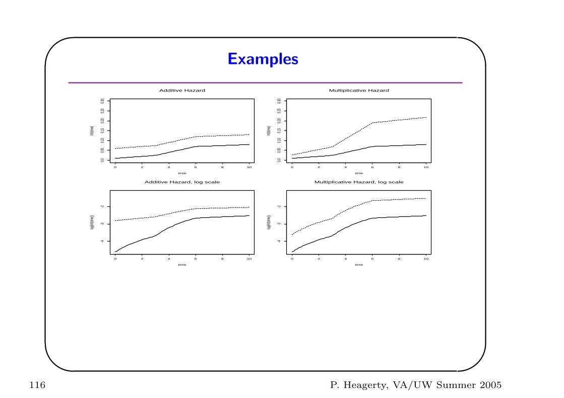
Hazard Models
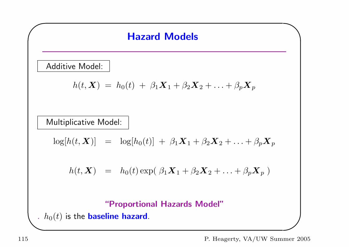
Additive Model:
h(t,X) = h0(t) + β1X1 + β2X2 + . . . + βpXp
Multiplicative Model:
log[h(t, X)] = log[h0(t)] + β1X1 + β2X2 + . . . + βpXp
h(t,X) = h0(t) exp( β1X1 + β2X2 + . . . + βpXp )
“Proportional Hazards Model”
. h0(t) is the baseline hazard.
115 P. Heagerty, VA/UW Summer 2005
'
&
$
%
Examples
time
h0(tim
e)
0 2 4 6 8 10
0.00.0
50.1
00.1
50.2
00.2
50.3
0
Additive Hazard
time
h0(tim
e)
0 2 4 6 8 10
0.00.0
50.1
00.1
50.2
00.2
50.3
0
Multiplicative Hazard
time
log(h0
(time))
0 2 4 6 8 10
-4-3
-2
Additive Hazard, log scale
time
log(h0
(time))
0 2 4 6 8 10
-4-3
-2
Multiplicative Hazard, log scale
116 P. Heagerty, VA/UW Summer 2005
'
&
$
%
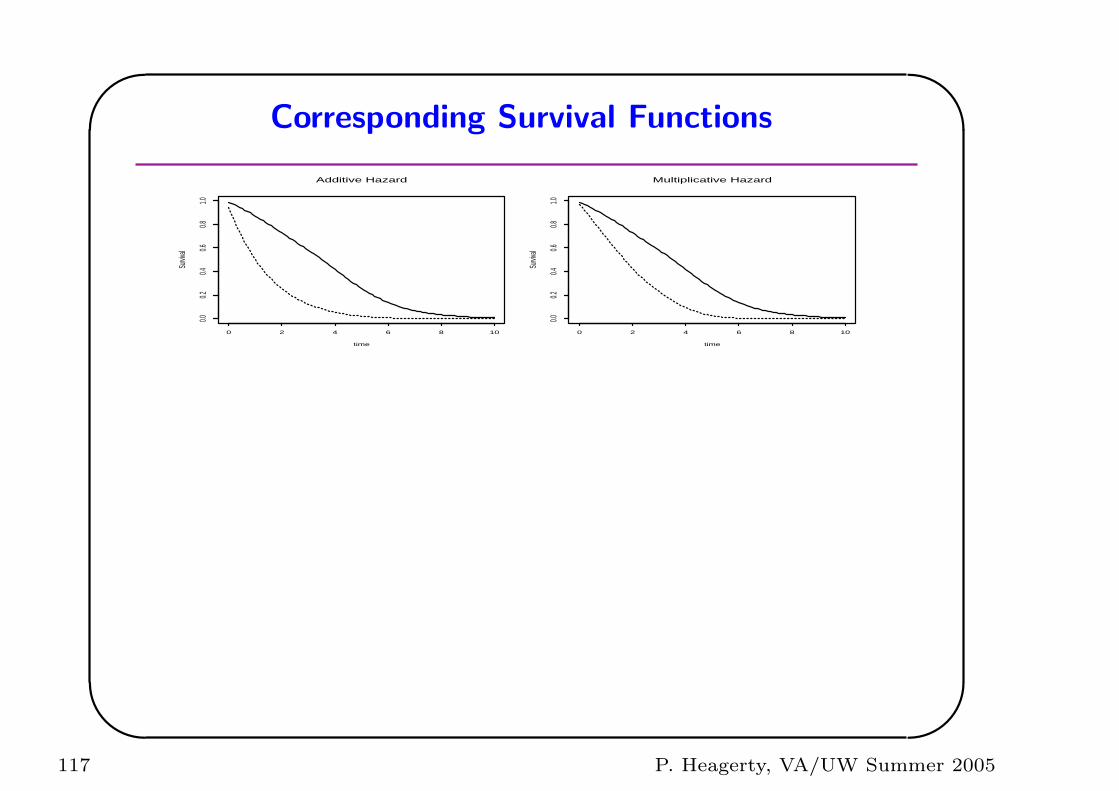
Corresponding Survival Functions
time
Survi
val
0 2 4 6 8 10
0.00.2
0.40.6
0.81.0
Additive Hazard
time
Survi
val
0 2 4 6 8 10
0.00.2
0.40.6
0.81.0
Multiplicative Hazard
117 P. Heagerty, VA/UW Summer 2005
'
&
$
%
Cox’s Proportional Hazards Model
1. With the PH model we can handle several covariates
simultaneously.
2. The construction of the model and the interpretation of the terms
in the model is just like linear regression and logistic regression,
except now we model hazard ratios.
3. The main concept is that we are using Cox regression to obtain
comparisons between different groups, formed on the basis of
covariates, in terms of their instantaneous probability of dying at
any point in time. In other words, we model hazard rates.
118 P. Heagerty, VA/UW Summer 2005
'
&
$
%
Cox’s Proportional Hazards Model
• One amazing contribution of Cox (1972) was an elegant likelihood
method that allows estimation of the parameters of interest, β,
without having to estimate the baseline hazard, h0(t). This type
of model is known as “semi-parametric” since there is a part of
the model that is parametric (β), and part of the model that is
left unspecified (the non-parametric part is h0(t)). The likelihood
that Cox constructed is called a “partial likelihood”.
119 P. Heagerty, VA/UW Summer 2005
'
&
$
%
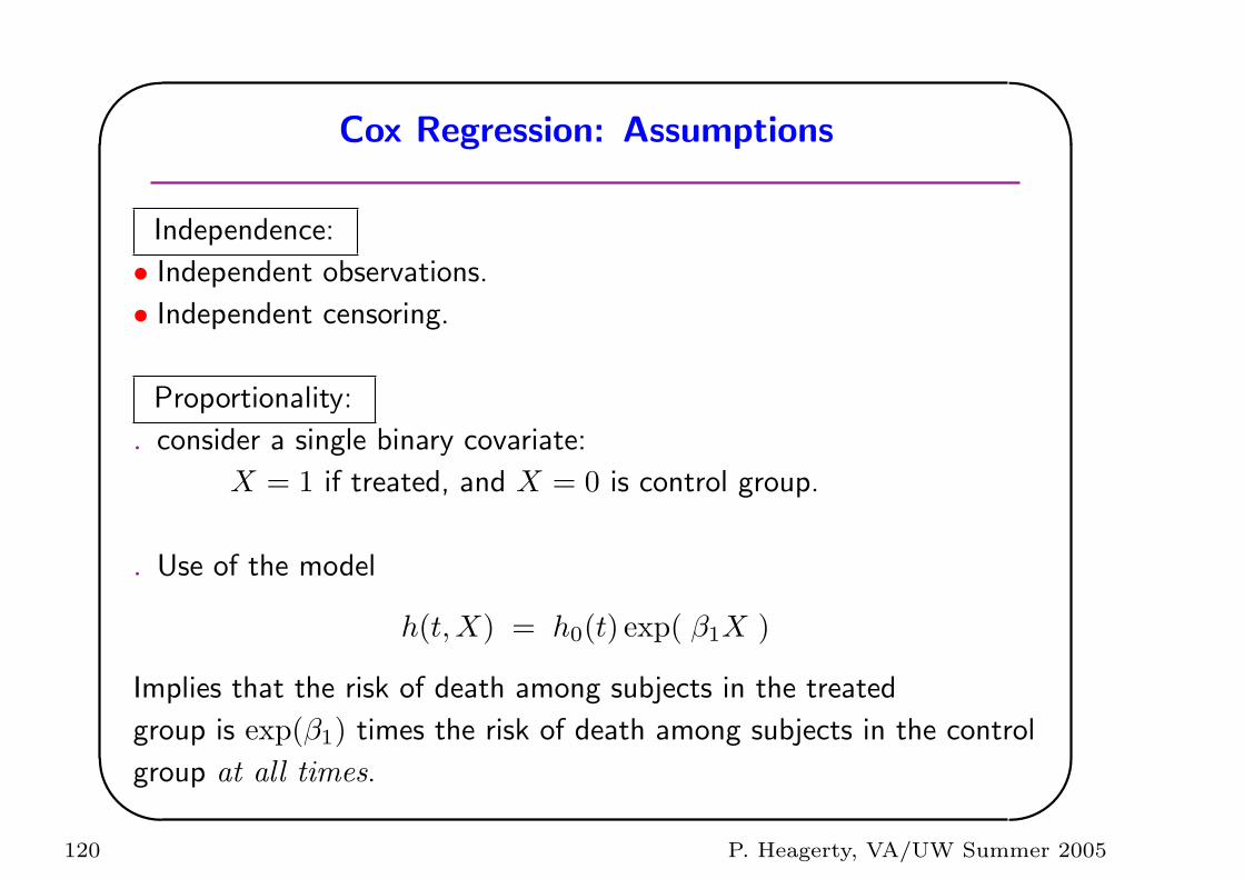
Cox Regression: Assumptions
Independence:
• Independent observations.
• Independent censoring.
Proportionality:
. consider a single binary covariate:
X = 1 if treated, and X = 0 is control group.
. Use of the model
h(t,X) = h0(t) exp( β1X )
Implies that the risk of death among subjects in the treated
group is exp(β1) times the risk of death among subjects in the control
group at all times.
120 P. Heagerty, VA/UW Summer 2005
'
&
$
%
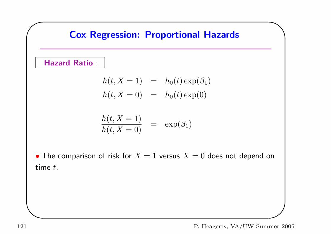
Cox Regression: Proportional Hazards
Hazard Ratio :
h(t,X = 1) = h0(t) exp(β1)
h(t,X = 0) = h0(t) exp(0)
h(t,X = 1)h(t,X = 0)
= exp(β1)
• The comparison of risk for X = 1 versus X = 0 does not depend on
time t.
121 P. Heagerty, VA/UW Summer 2005
'
&
$
%
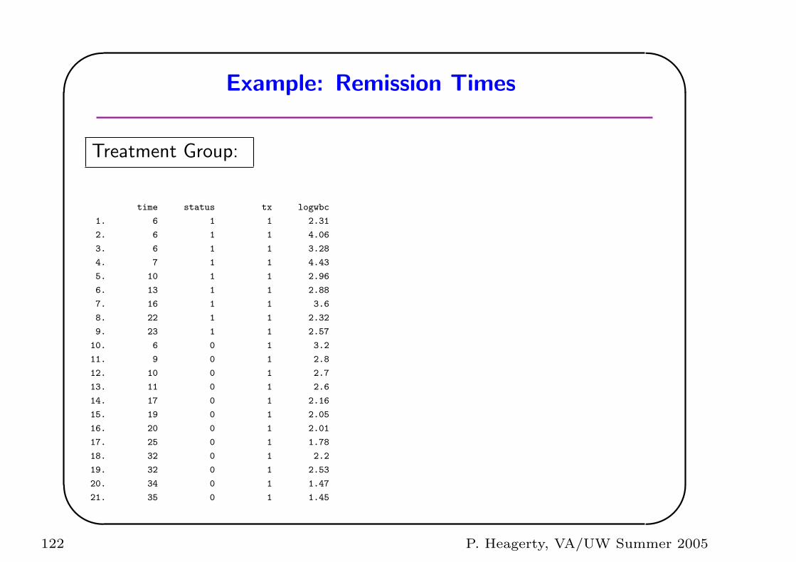
Example: Remission Times
Treatment Group:
time status tx logwbc
1. 6 1 1 2.31
2. 6 1 1 4.06
3. 6 1 1 3.28
4. 7 1 1 4.43
5. 10 1 1 2.96
6. 13 1 1 2.88
7. 16 1 1 3.6
8. 22 1 1 2.32
9. 23 1 1 2.57
10. 6 0 1 3.2
11. 9 0 1 2.8
12. 10 0 1 2.7
13. 11 0 1 2.6
14. 17 0 1 2.16
15. 19 0 1 2.05
16. 20 0 1 2.01
17. 25 0 1 1.78
18. 32 0 1 2.2
19. 32 0 1 2.53
20. 34 0 1 1.47
21. 35 0 1 1.45
122 P. Heagerty, VA/UW Summer 2005
'
&
$
%
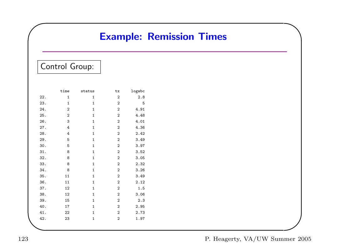
Example: Remission Times
Control Group:
time status tx logwbc
22. 1 1 2 2.8
23. 1 1 2 5
24. 2 1 2 4.91
25. 2 1 2 4.48
26. 3 1 2 4.01
27. 4 1 2 4.36
28. 4 1 2 2.42
29. 5 1 2 3.49
30. 5 1 2 3.97
31. 8 1 2 3.52
32. 8 1 2 3.05
33. 8 1 2 2.32
34. 8 1 2 3.26
35. 11 1 2 3.49
36. 11 1 2 2.12
37. 12 1 2 1.5
38. 12 1 2 3.06
39. 15 1 2 2.3
40. 17 1 2 2.95
41. 22 1 2 2.73
42. 23 1 2 1.97
123 P. Heagerty, VA/UW Summer 2005
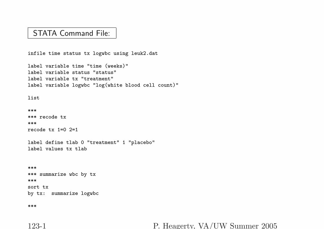
STATA Command File:
infile time status tx logwbc using leuk2.dat
label variable time "time (weeks)"label variable status "status"label variable tx "treatment"label variable logwbc "log(white blood cell count)"
list
****** recode tx***recode tx 1=0 2=1
label define tlab 0 "treatment" 1 "placebo"label values tx tlab
****** summarize wbc by tx***sort txby tx: summarize logwbc
***
123-1 P. Heagerty, VA/UW Summer 2005
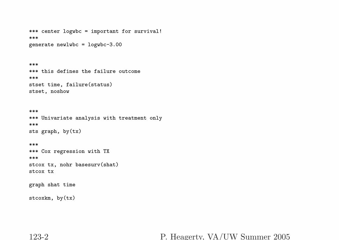
*** center logwbc = important for survival!***generate newlwbc = logwbc-3.00
****** this defines the failure outcome***stset time, failure(status)stset, noshow
****** Univariate analysis with treatment only***sts graph, by(tx)
****** Cox regression with TX***stcox tx, nohr basesurv(shat)stcox tx
graph shat time
stcoxkm, by(tx)
123-2 P. Heagerty, VA/UW Summer 2005
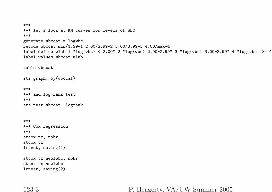
****** let’s look at KM curves for levels of WBC***generate wbccat = logwbcrecode wbccat min/1.99=1 2.00/2.99=2 3.00/3.99=3 4.00/max=4label define wlab 1 "log(wbc) < 2.00" 2 "log(wbc) 2.00-2.99" 3 "log(wbc) 3.00-3.99" 4 "log(wbc) >= 4.00"label values wbccat wlab
table wbccat
sts graph, by(wbccat)
****** and log-rank test***sts test wbccat, logrank
****** Cox regression***stcox tx, nohrstcox txlrtest, saving(1)
stcox tx newlwbc, nohrstcox tx newlwbclrtest, saving(2)
123-3 P. Heagerty, VA/UW Summer 2005
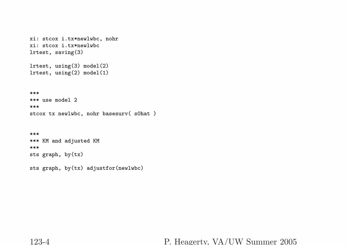
xi: stcox i.tx*newlwbc, nohrxi: stcox i.tx*newlwbclrtest, saving(3)
lrtest, using(3) model(2)lrtest, using(2) model(1)
****** use model 2***stcox tx newlwbc, nohr basesurv( s0hat )
****** KM and adjusted KM***sts graph, by(tx)
sts graph, by(tx) adjustfor(newlwbc)
123-4 P. Heagerty, VA/UW Summer 2005
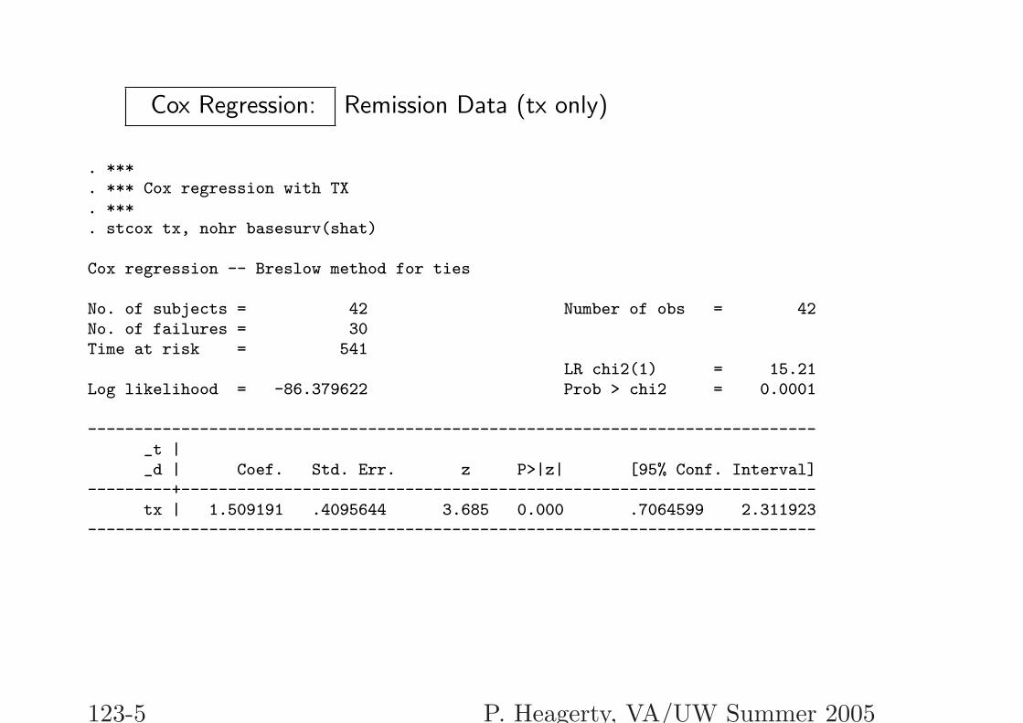
Cox Regression: Remission Data (tx only)
. ***
. *** Cox regression with TX
. ***
. stcox tx, nohr basesurv(shat)
Cox regression -- Breslow method for ties
No. of subjects = 42 Number of obs = 42No. of failures = 30Time at risk = 541
LR chi2(1) = 15.21Log likelihood = -86.379622 Prob > chi2 = 0.0001
------------------------------------------------------------------------------_t |_d | Coef. Std. Err. z P>|z| [95% Conf. Interval]
---------+--------------------------------------------------------------------tx | 1.509191 .4095644 3.685 0.000 .7064599 2.311923
------------------------------------------------------------------------------
123-5 P. Heagerty, VA/UW Summer 2005
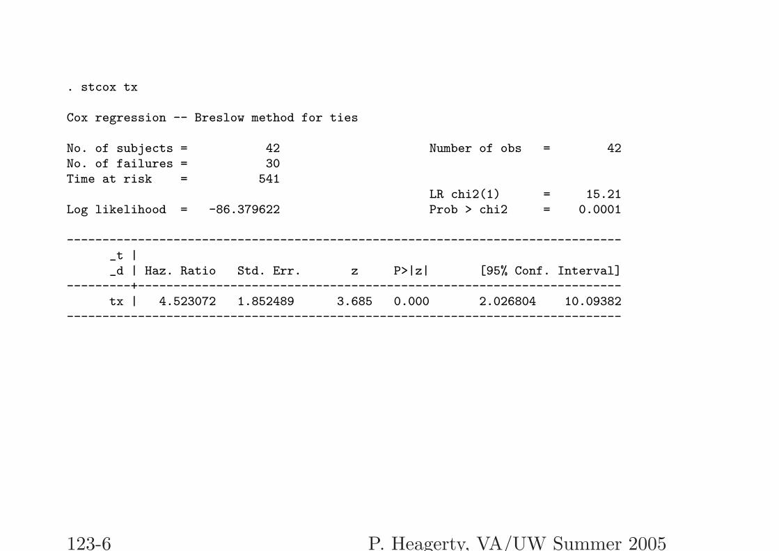
. stcox tx
Cox regression -- Breslow method for ties
No. of subjects = 42 Number of obs = 42No. of failures = 30Time at risk = 541
LR chi2(1) = 15.21Log likelihood = -86.379622 Prob > chi2 = 0.0001
------------------------------------------------------------------------------_t |_d | Haz. Ratio Std. Err. z P>|z| [95% Conf. Interval]
---------+--------------------------------------------------------------------tx | 4.523072 1.852489 3.685 0.000 2.026804 10.09382
------------------------------------------------------------------------------
123-6 P. Heagerty, VA/UW Summer 2005
'
&
$
%
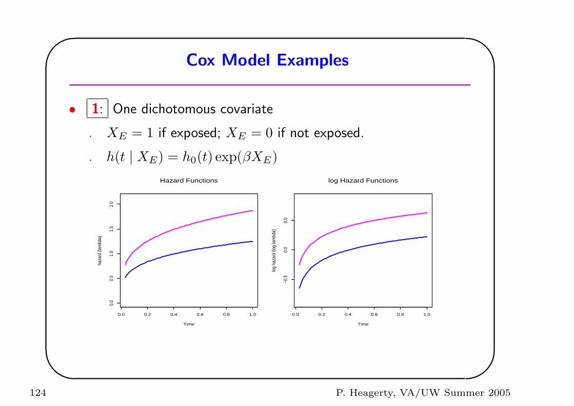
Cox Model Examples
• 1: One dichotomous covariate
. XE = 1 if exposed; XE = 0 if not exposed.
. h(t | XE) = h0(t) exp(βXE)
Time
haza
rd (l
ambd
a)
0.0 0.2 0.4 0.6 0.8 1.0
0.0
0.5
1.0
1.5
2.0
Hazard Functions
Time
log
haza
rd (l
og la
mbd
a)
0.0 0.2 0.4 0.6 0.8 1.0
−0.5
0.0
0.5
log Hazard Functions
124 P. Heagerty, VA/UW Summer 2005
'
&
$
%
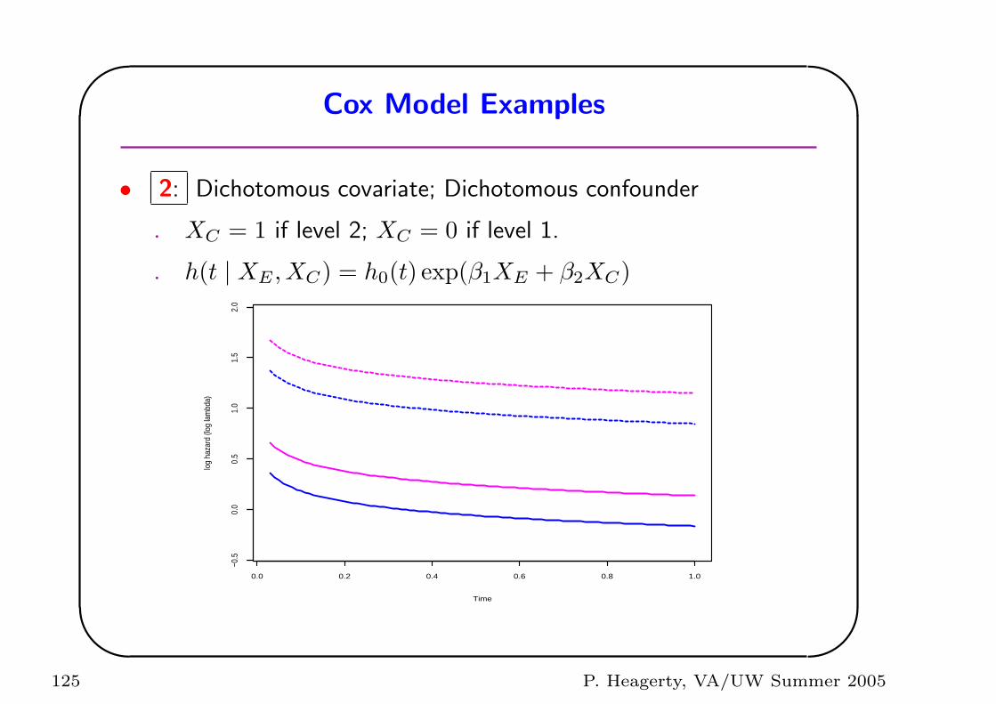
Cox Model Examples
• 2: Dichotomous covariate; Dichotomous confounder
. XC = 1 if level 2; XC = 0 if level 1.
. h(t | XE , XC) = h0(t) exp(β1XE + β2XC)
Time
log
haza
rd (l
og la
mbd
a)
0.0 0.2 0.4 0.6 0.8 1.0
−0.5
0.0
0.5
1.0
1.5
2.0
125 P. Heagerty, VA/UW Summer 2005
'
&
$
%
Cox Model Examples
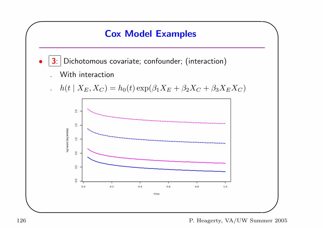
• 3: Dichotomous covariate; confounder; (interaction)
. With interaction
. h(t | XE , XC) = h0(t) exp(β1XE + β2XC + β3XEXC)
Time
log
haza
rd (l
og la
mbd
a)
0.0 0.2 0.4 0.6 0.8 1.0
−0.5
0.0
0.5
1.0
1.5
2.0
126 P. Heagerty, VA/UW Summer 2005
'
&
$
%
Cox Model Examples
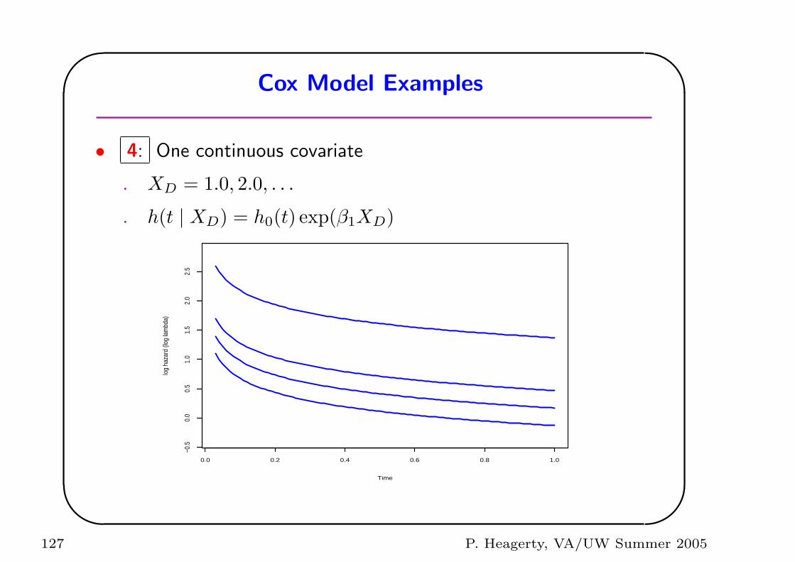
• 4: One continuous covariate
. XD = 1.0, 2.0, . . .
. h(t | XD) = h0(t) exp(β1XD)
Time
log
haza
rd (l
og la
mbd
a)
0.0 0.2 0.4 0.6 0.8 1.0
−0.5
0.0
0.5
1.0
1.5
2.0
2.5
127 P. Heagerty, VA/UW Summer 2005
'
&
$
%
Cox Model Examples
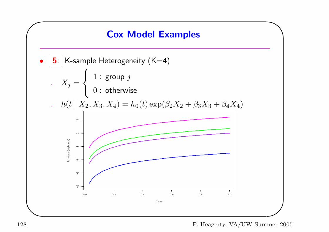
• 5: K-sample Heterogeneity (K=4)
. Xj =
1 : group j
0 : otherwise
. h(t | X2, X3, X4) = h0(t) exp(β2X2 + β3X3 + β4X4)
Time
log
haza
rd (l
og la
mbd
a)
0.0 0.2 0.4 0.6 0.8 1.0
−2−1
01
23
128 P. Heagerty, VA/UW Summer 2005
'
&
$
%
Cox Model Examples
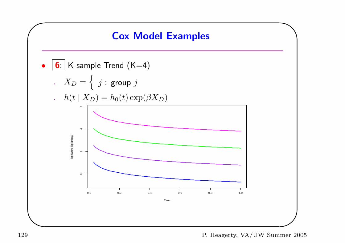
• 6: K-sample Trend (K=4)
. XD ={
j : group j
. h(t | XD) = h0(t) exp(βXD)
Time
log
haza
rd (l
og la
mbd
a)
0.0 0.2 0.4 0.6 0.8 1.0
02
46
129 P. Heagerty, VA/UW Summer 2005
'
&
$
%
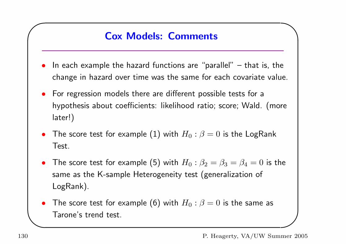
Cox Models: Comments
• In each example the hazard functions are “parallel” – that is, the
change in hazard over time was the same for each covariate value.
• For regression models there are different possible tests for a
hypothesis about coefficients: likelihood ratio; score; Wald. (more
later!)
• The score test for example (1) with H0 : β = 0 is the LogRank
Test.
• The score test for example (5) with H0 : β2 = β3 = β4 = 0 is the
same as the K-sample Heterogeneity test (generalization of
LogRank).
• The score test for example (6) with H0 : β = 0 is the same as
Tarone’s trend test.
130 P. Heagerty, VA/UW Summer 2005
'
&
$
%
Summary
1. Interpretation of the hazard.
2. Definition of the cumulative hazard.
3. S(t) ⇐⇒ H(t) ⇐⇒ h(t)
4. Examples using common parametric models (exponential model,
weibull model).
5. Cox proportional hazards model:
h(t, X) = h0(t) exp( β1X1 + β2X2 + . . . )
6. Estimation and inference for hazard ratio regression parameters.
131 P. Heagerty, VA/UW Summer 2005
'
&
$
%
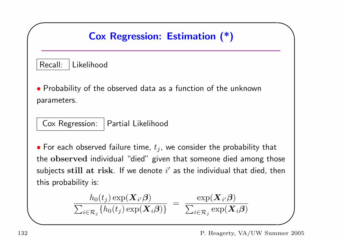
Cox Regression: Estimation (*)
Recall: Likelihood
• Probability of the observed data as a function of the unknown
parameters.
Cox Regression: Partial Likelihood
• For each observed failure time, tj , we consider the probability that
the observed individual “died” given that someone died among those
subjects still at risk. If we denote i′ as the individual that died, then
this probability is:
h0(tj) exp(Xi′β)∑i∈Rj
{h0(tj) exp(Xiβ)} =exp(Xi′β)∑
i∈Rjexp(Xiβ)
132 P. Heagerty, VA/UW Summer 2005
'
&
$
%
where
Rj = those subjects still at-risk at time tj
• The partial likelihood then considers all observed failure times. The
partial likelihood is the product of these probabilities for all observed
failure times, tj .
133 P. Heagerty, VA/UW Summer 2005
'
&
$
%
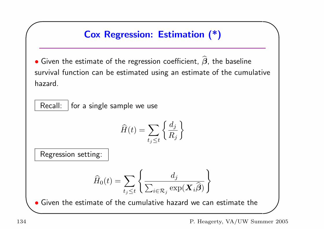
Cox Regression: Estimation (*)
• Given the estimate of the regression coefficient, β, the baseline
survival function can be estimated using an estimate of the cumulative
hazard.
Recall: for a single sample we use
H(t) =∑
tj≤t
{dj
Rj
}
Regression setting:
H0(t) =∑
tj≤t
{dj∑
i∈Rjexp(Xiβ)
}
• Given the estimate of the cumulative hazard we can estimate the
134 P. Heagerty, VA/UW Summer 2005
'
&
$
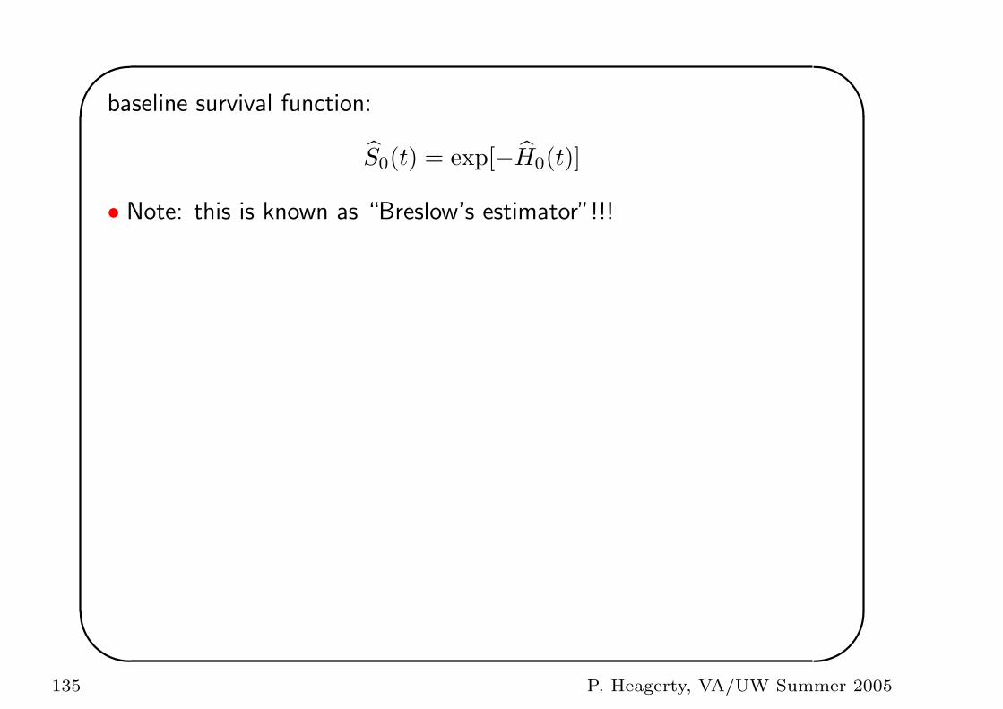
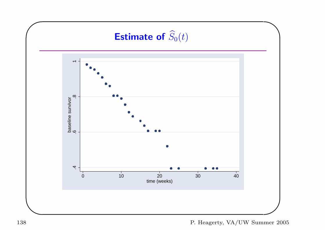
%
baseline survival function:
S0(t) = exp[−H0(t)]
• Note: this is known as “Breslow’s estimator”!!!
135 P. Heagerty, VA/UW Summer 2005
'
&
$
%
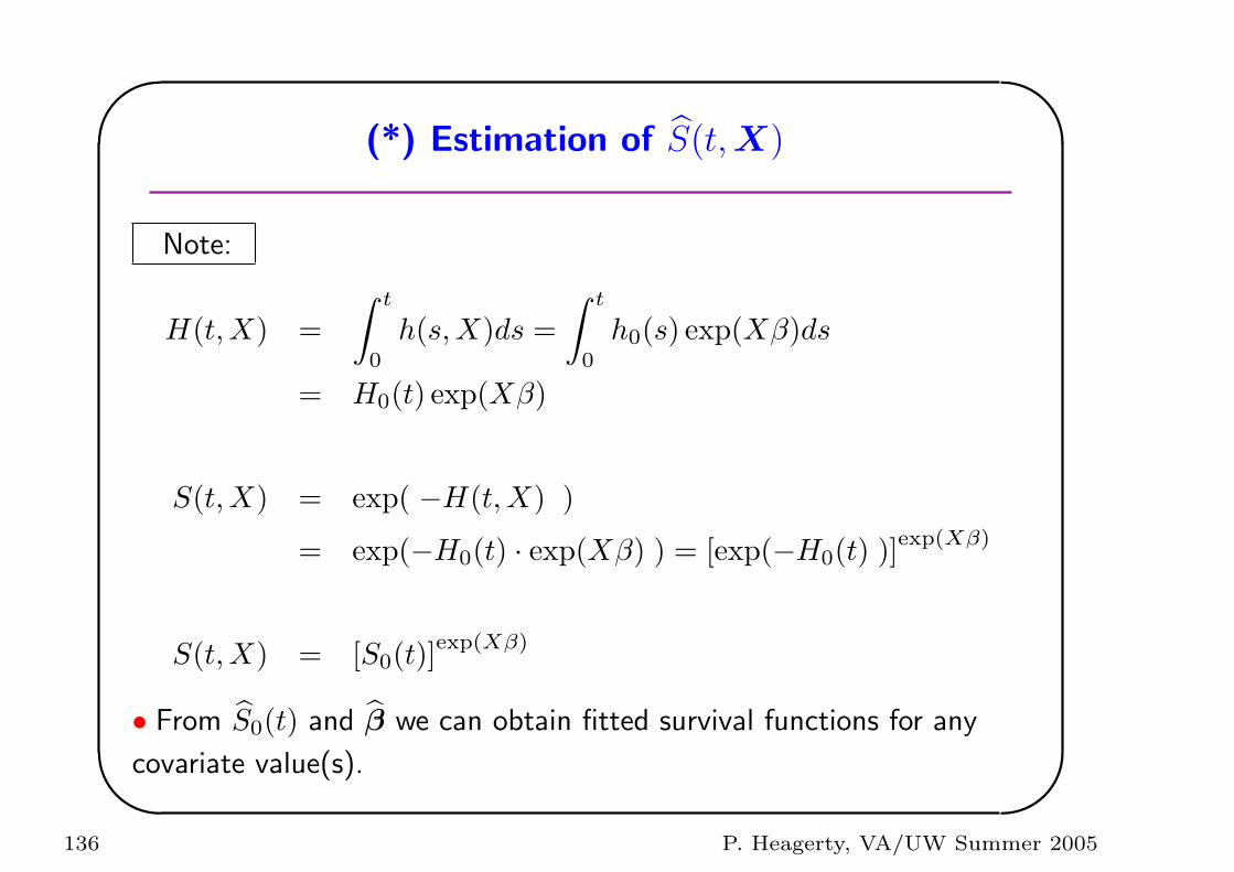
(*) Estimation of S(t, X)
Note:
H(t,X) =∫ t
0
h(s, X)ds =∫ t
0
h0(s) exp(Xβ)ds
= H0(t) exp(Xβ)
S(t,X) = exp( −H(t,X) )
= exp(−H0(t) · exp(Xβ) ) = [exp(−H0(t) )]exp(Xβ)
S(t,X) = [S0(t)]exp(Xβ)
• From S0(t) and β we can obtain fitted survival functions for any
covariate value(s).
136 P. Heagerty, VA/UW Summer 2005
'
&
$
%
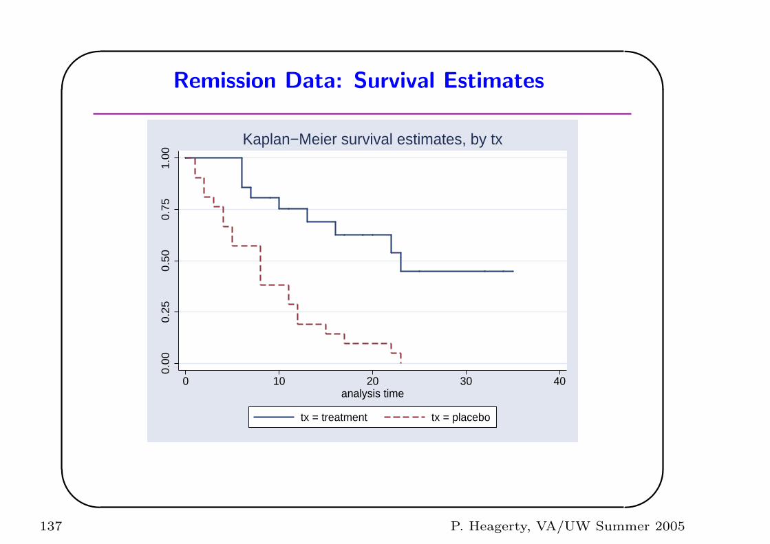
Remission Data: Survival Estimates
0.00
0.25
0.50
0.75
1.00
0 10 20 30 40analysis time
tx = treatment tx = placebo
Kaplan−Meier survival estimates, by tx
137 P. Heagerty, VA/UW Summer 2005
'
&
$
%
Estimate of S0(t)
.4.6
.81
base
line
surv
ivor
0 10 20 30 40time (weeks)
138 P. Heagerty, VA/UW Summer 2005

'
&
$
%
Observed (KM) and Fitted (Cox model)
0.00
0.20
0.40
0.60
0.80
1.00
Sur
viva
l Pro
babi
lity
0 10 20 30 40analysis time
Observed: tx = treatment Observed: tx = placeboPredicted: tx = treatment Predicted: tx = placebo
139 P. Heagerty, VA/UW Summer 2005
'
&
$
%
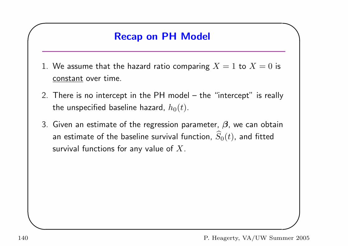
Recap on PH Model
1. We assume that the hazard ratio comparing X = 1 to X = 0 is
constant over time.
2. There is no intercept in the PH model – the “intercept” is really
the unspecified baseline hazard, h0(t).
3. Given an estimate of the regression parameter, β, we can obtain
an estimate of the baseline survival function, S0(t), and fitted
survival functions for any value of X.
140 P. Heagerty, VA/UW Summer 2005
'
&
$
%
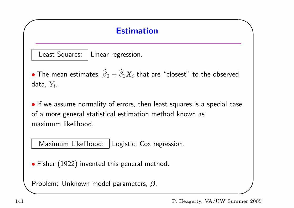
Estimation
Least Squares: Linear regression.
• The mean estimates, β0 + β1Xi that are “closest” to the observed
data, Yi.
• If we assume normality of errors, then least squares is a special case
of a more general statistical estimation method known as
maximum likelihood.
Maximum Likelihood: Logistic, Cox regression.
• Fisher (1922) invented this general method.
Problem: Unknown model parameters, β.
141 P. Heagerty, VA/UW Summer 2005
'
&
$
%
Set-up: Write the probability of the data, Y , in terms of the model
parameter and the data, P (Y , β).
Solution: Choose as your estimate the value of the unknown
parameter that makes your data look as likely as possible. Pick β that
puts the largest possible probability on your data.
142 P. Heagerty, VA/UW Summer 2005
'
&
$
%
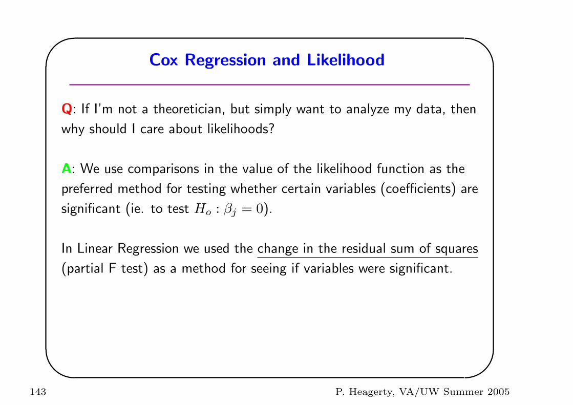
Cox Regression and Likelihood
Q: If I’m not a theoretician, but simply want to analyze my data, then
why should I care about likelihoods?
A: We use comparisons in the value of the likelihood function as the
preferred method for testing whether certain variables (coefficients) are
significant (ie. to test Ho : βj = 0).
In Linear Regression we used the change in the residual sum of squares
(partial F test) as a method for seeing if variables were significant.
143 P. Heagerty, VA/UW Summer 2005
'
&
$
%
Cox Regression and Likelihood
In Logistic Regression we will use the change in the log likelihood as a
method for seeing if variables are significant.
In Cox Regression we will use the change in the log likelihood as a
method for seeing if variables are significant.
144 P. Heagerty, VA/UW Summer 2005
'
&
$
%
Cox Regression: Inference
• “Nested” models
• Maximized log likelihood, log L, & Likelihood Ratio Tests
• β and standard errors – Wald Tests
• Inference for linear combinations of β
145 P. Heagerty, VA/UW Summer 2005
'
&
$
%
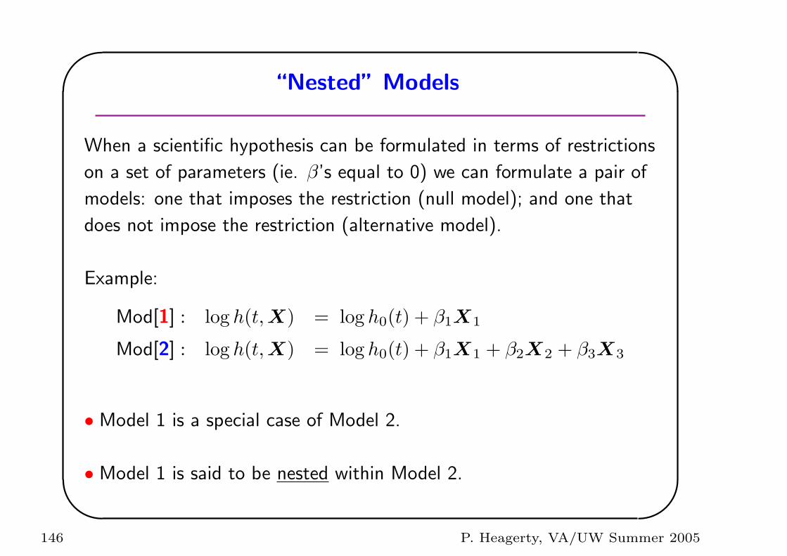
“Nested” Models
When a scientific hypothesis can be formulated in terms of restrictions
on a set of parameters (ie. β’s equal to 0) we can formulate a pair of
models: one that imposes the restriction (null model); and one that
does not impose the restriction (alternative model).
Example:
Mod[1] : log h(t, X) = log h0(t) + β1X1
Mod[2] : log h(t, X) = log h0(t) + β1X1 + β2X2 + β3X3
• Model 1 is a special case of Model 2.
• Model 1 is said to be nested within Model 2.
146 P. Heagerty, VA/UW Summer 2005
'
&
$
%
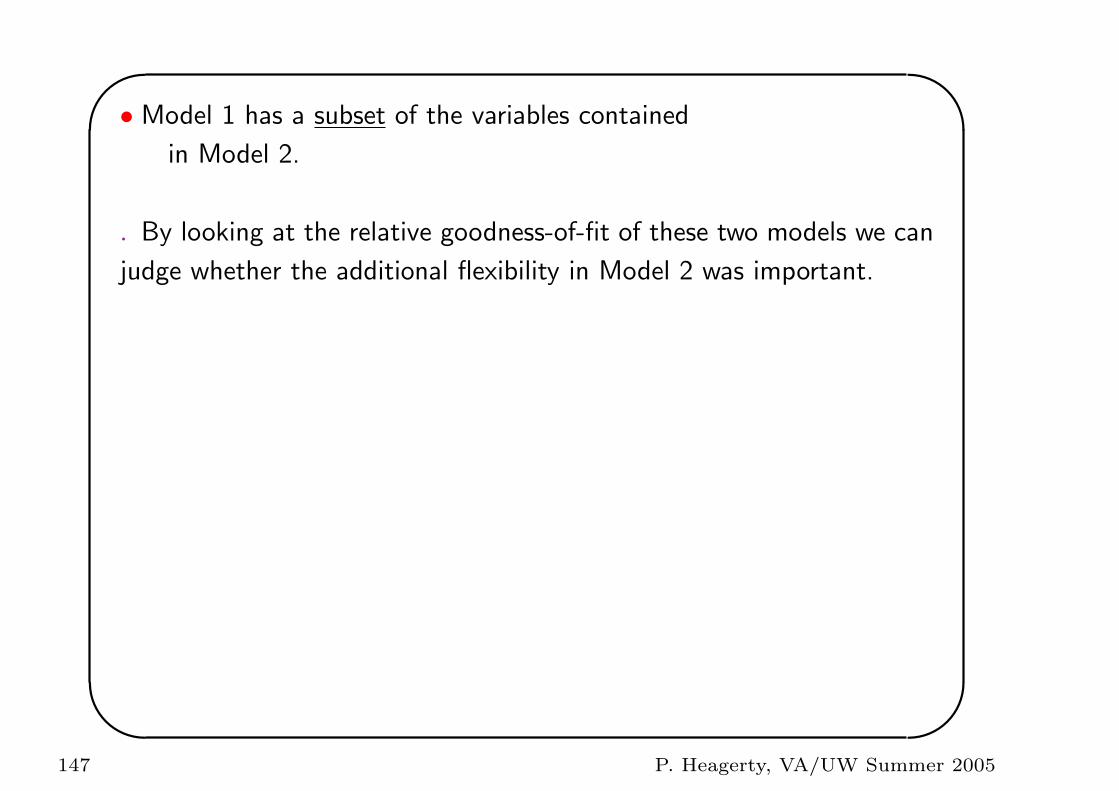
• Model 1 has a subset of the variables contained
in Model 2.
. By looking at the relative goodness-of-fit of these two models we can
judge whether the additional flexibility in Model 2 was important.
147 P. Heagerty, VA/UW Summer 2005
'
&
$
%
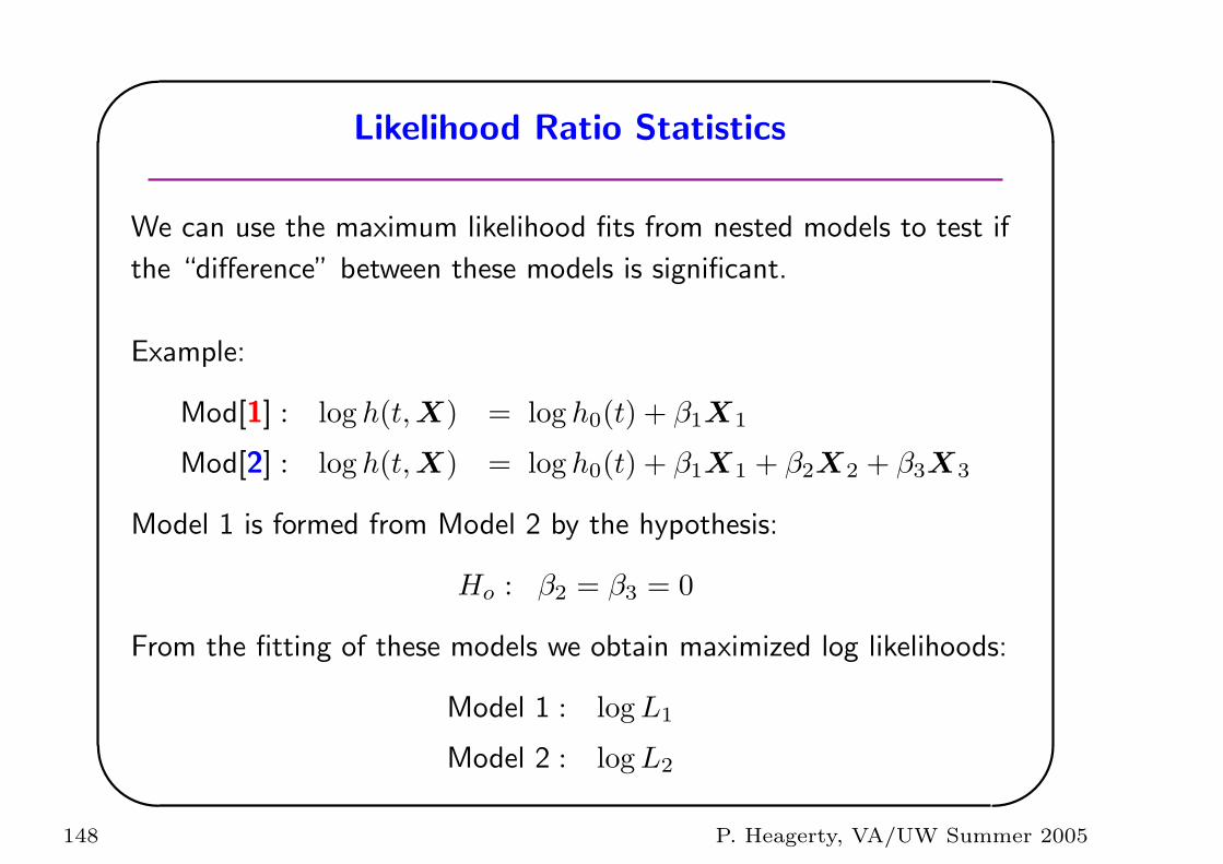
Likelihood Ratio Statistics
We can use the maximum likelihood fits from nested models to test if
the “difference” between these models is significant.
Example:
Mod[1] : log h(t, X) = log h0(t) + β1X1
Mod[2] : log h(t, X) = log h0(t) + β1X1 + β2X2 + β3X3
Model 1 is formed from Model 2 by the hypothesis:
Ho : β2 = β3 = 0
From the fitting of these models we obtain maximized log likelihoods:
Model 1 : log L1
Model 2 : log L2
148 P. Heagerty, VA/UW Summer 2005
'
&
$
%
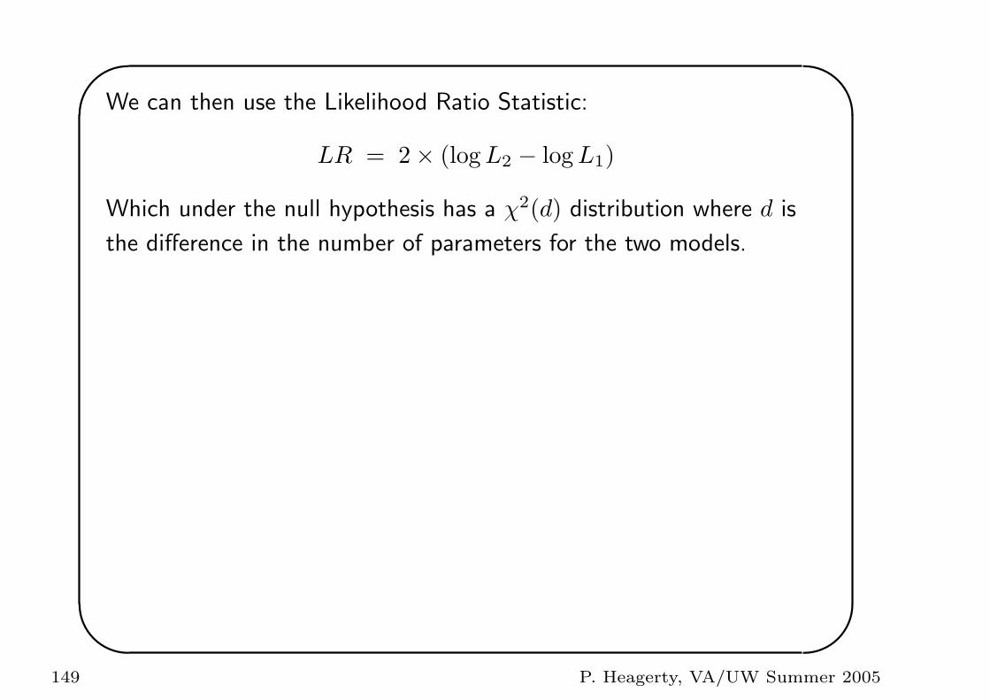
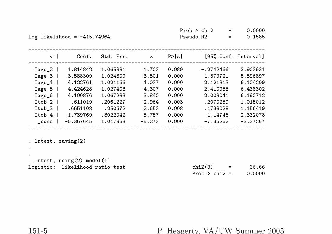
We can then use the Likelihood Ratio Statistic:
LR = 2× (log L2 − log L1)
Which under the null hypothesis has a χ2(d) distribution where d is
the difference in the number of parameters for the two models.
149 P. Heagerty, VA/UW Summer 2005
'
&
$
%
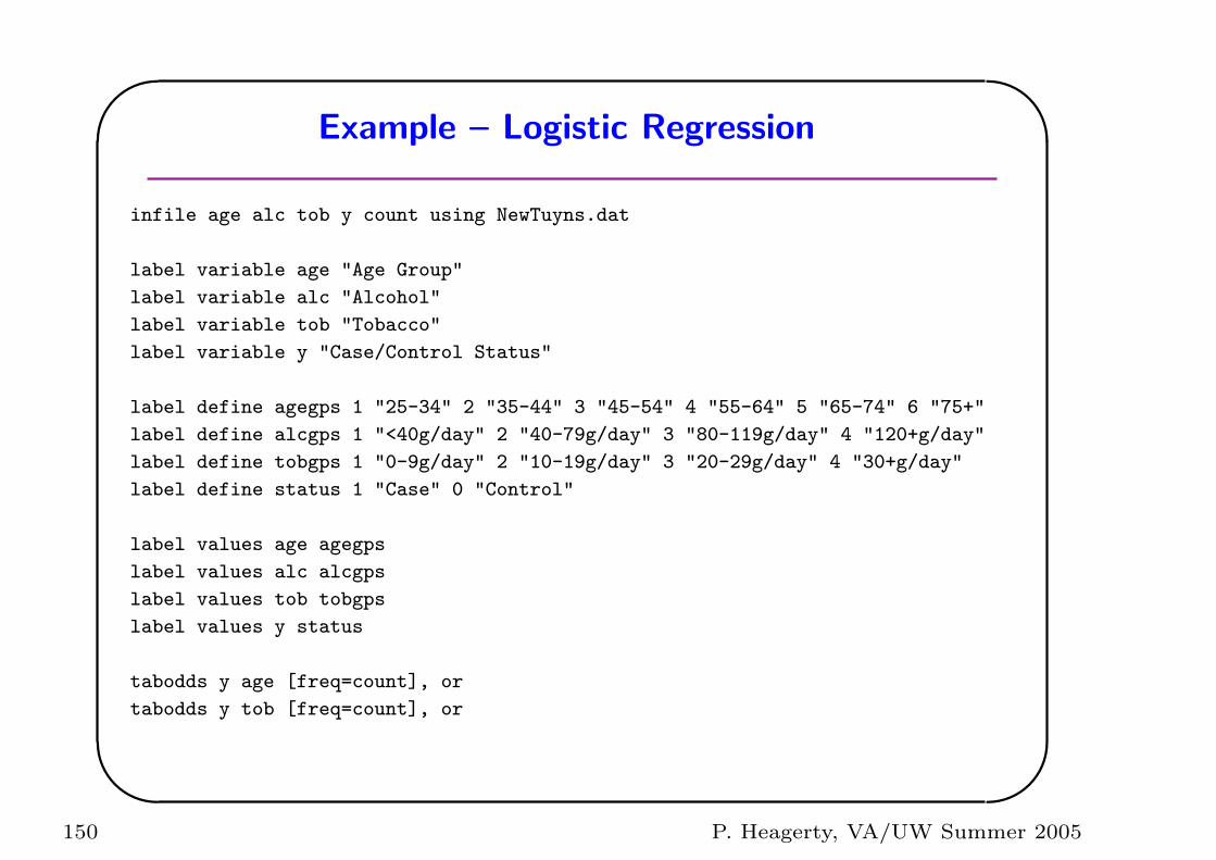
Example – Logistic Regression
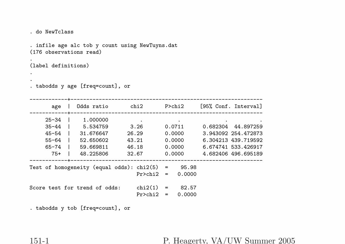
infile age alc tob y count using NewTuyns.dat
label variable age "Age Group"
label variable alc "Alcohol"
label variable tob "Tobacco"
label variable y "Case/Control Status"
label define agegps 1 "25-34" 2 "35-44" 3 "45-54" 4 "55-64" 5 "65-74" 6 "75+"
label define alcgps 1 "<40g/day" 2 "40-79g/day" 3 "80-119g/day" 4 "120+g/day"
label define tobgps 1 "0-9g/day" 2 "10-19g/day" 3 "20-29g/day" 4 "30+g/day"
label define status 1 "Case" 0 "Control"
label values age agegps
label values alc alcgps
label values tob tobgps
label values y status
tabodds y age [freq=count], or
tabodds y tob [freq=count], or
150 P. Heagerty, VA/UW Summer 2005
'
&
$
%
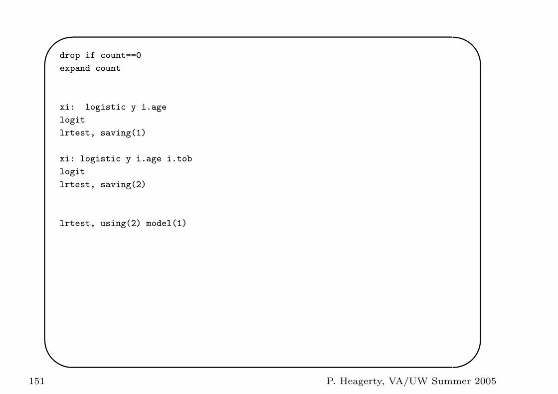
drop if count==0
expand count
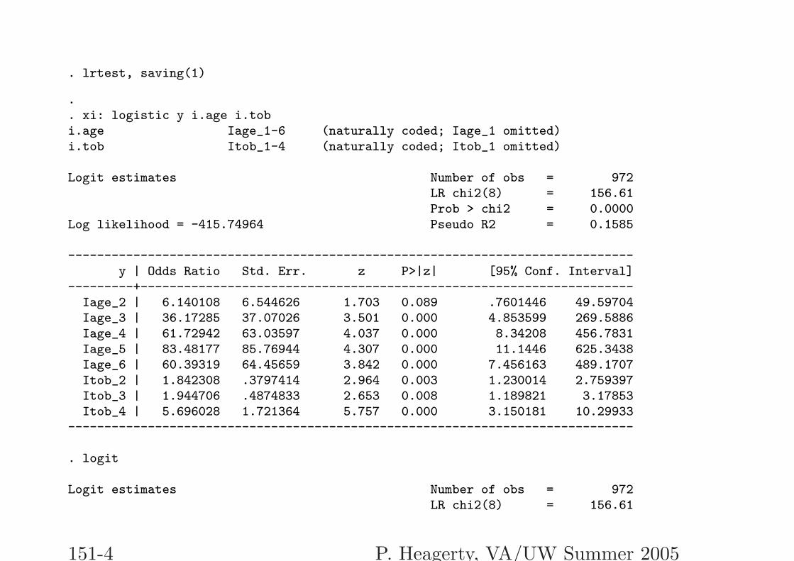
xi: logistic y i.age
logit
lrtest, saving(1)
xi: logistic y i.age i.tob
logit
lrtest, saving(2)
lrtest, using(2) model(1)
151 P. Heagerty, VA/UW Summer 2005
. do NewTclass
. infile age alc tob y count using NewTuyns.dat(176 observations read).(label definitions)... tabodds y age [freq=count], or
------------+-------------------------------------------------------------age | Odds ratio chi2 P>chi2 [95% Conf. Interval]
------------+-------------------------------------------------------------25-34 | 1.000000 . . . .35-44 | 5.534759 3.26 0.0711 0.682304 44.89725945-54 | 31.676647 26.29 0.0000 3.943092 254.47287355-64 | 52.650602 43.21 0.0000 6.304213 439.71959265-74 | 59.669811 46.18 0.0000 6.674741 533.426917
75+ | 48.225806 32.67 0.0000 4.682406 496.695189------------+-------------------------------------------------------------Test of homogeneity (equal odds): chi2(5) = 95.98
Pr>chi2 = 0.0000
Score test for trend of odds: chi2(1) = 82.57Pr>chi2 = 0.0000
. tabodds y tob [freq=count], or
151-1 P. Heagerty, VA/UW Summer 2005
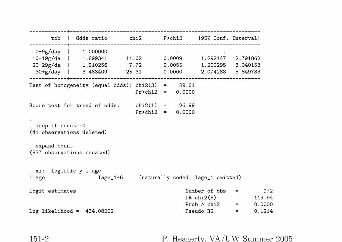
------------+-------------------------------------------------------------tob | Odds ratio chi2 P>chi2 [95% Conf. Interval]
------------+-------------------------------------------------------------0-9g/day | 1.000000 . . . .
10-19g/da | 1.899341 11.02 0.0009 1.292147 2.79186220-29g/da | 1.910256 7.72 0.0055 1.200295 3.04015330+g/day | 3.483409 25.31 0.0000 2.074288 5.849783
------------+-------------------------------------------------------------Test of homogeneity (equal odds): chi2(3) = 29.61
Pr>chi2 = 0.0000
Score test for trend of odds: chi2(1) = 26.99Pr>chi2 = 0.0000
.
. drop if count==0(41 observations deleted)
. expand count(837 observations created)
. xi: logistic y i.agei.age Iage_1-6 (naturally coded; Iage_1 omitted)
Logit estimates Number of obs = 972LR chi2(5) = 119.94Prob > chi2 = 0.0000
Log likelihood = -434.08202 Pseudo R2 = 0.1214
151-2 P. Heagerty, VA/UW Summer 2005
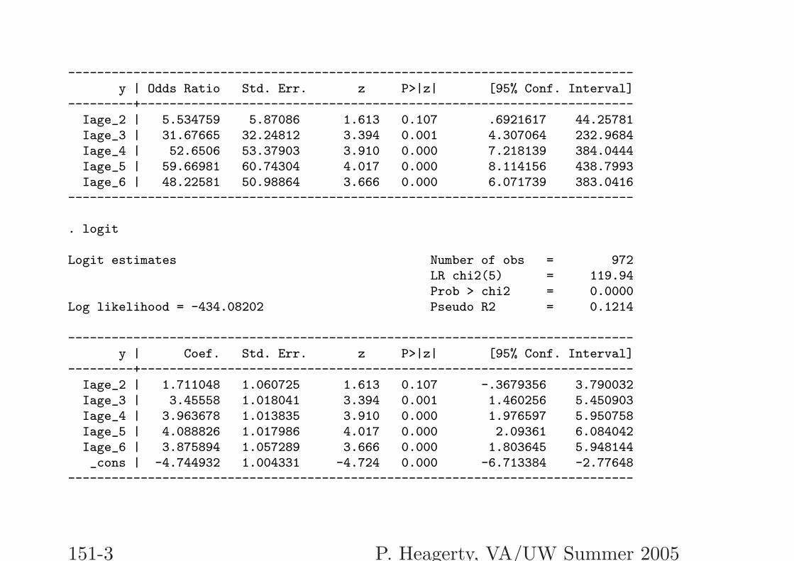
------------------------------------------------------------------------------y | Odds Ratio Std. Err. z P>|z| [95% Conf. Interval]
---------+--------------------------------------------------------------------Iage_2 | 5.534759 5.87086 1.613 0.107 .6921617 44.25781Iage_3 | 31.67665 32.24812 3.394 0.001 4.307064 232.9684Iage_4 | 52.6506 53.37903 3.910 0.000 7.218139 384.0444Iage_5 | 59.66981 60.74304 4.017 0.000 8.114156 438.7993Iage_6 | 48.22581 50.98864 3.666 0.000 6.071739 383.0416
------------------------------------------------------------------------------
. logit
Logit estimates Number of obs = 972LR chi2(5) = 119.94Prob > chi2 = 0.0000
Log likelihood = -434.08202 Pseudo R2 = 0.1214
------------------------------------------------------------------------------y | Coef. Std. Err. z P>|z| [95% Conf. Interval]
---------+--------------------------------------------------------------------Iage_2 | 1.711048 1.060725 1.613 0.107 -.3679356 3.790032Iage_3 | 3.45558 1.018041 3.394 0.001 1.460256 5.450903Iage_4 | 3.963678 1.013835 3.910 0.000 1.976597 5.950758Iage_5 | 4.088826 1.017986 4.017 0.000 2.09361 6.084042Iage_6 | 3.875894 1.057289 3.666 0.000 1.803645 5.948144_cons | -4.744932 1.004331 -4.724 0.000 -6.713384 -2.77648
------------------------------------------------------------------------------
151-3 P. Heagerty, VA/UW Summer 2005
. lrtest, saving(1)
.
. xi: logistic y i.age i.tobi.age Iage_1-6 (naturally coded; Iage_1 omitted)i.tob Itob_1-4 (naturally coded; Itob_1 omitted)
Logit estimates Number of obs = 972LR chi2(8) = 156.61Prob > chi2 = 0.0000
Log likelihood = -415.74964 Pseudo R2 = 0.1585
------------------------------------------------------------------------------y | Odds Ratio Std. Err. z P>|z| [95% Conf. Interval]
---------+--------------------------------------------------------------------Iage_2 | 6.140108 6.544626 1.703 0.089 .7601446 49.59704Iage_3 | 36.17285 37.07026 3.501 0.000 4.853599 269.5886Iage_4 | 61.72942 63.03597 4.037 0.000 8.34208 456.7831Iage_5 | 83.48177 85.76944 4.307 0.000 11.1446 625.3438Iage_6 | 60.39319 64.45659 3.842 0.000 7.456163 489.1707Itob_2 | 1.842308 .3797414 2.964 0.003 1.230014 2.759397Itob_3 | 1.944706 .4874833 2.653 0.008 1.189821 3.17853Itob_4 | 5.696028 1.721364 5.757 0.000 3.150181 10.29933
------------------------------------------------------------------------------
. logit
Logit estimates Number of obs = 972LR chi2(8) = 156.61
151-4 P. Heagerty, VA/UW Summer 2005
Prob > chi2 = 0.0000Log likelihood = -415.74964 Pseudo R2 = 0.1585
------------------------------------------------------------------------------y | Coef. Std. Err. z P>|z| [95% Conf. Interval]
---------+--------------------------------------------------------------------Iage_2 | 1.814842 1.065881 1.703 0.089 -.2742466 3.903931Iage_3 | 3.588309 1.024809 3.501 0.000 1.579721 5.596897Iage_4 | 4.122761 1.021166 4.037 0.000 2.121313 6.124209Iage_5 | 4.424628 1.027403 4.307 0.000 2.410955 6.438302Iage_6 | 4.100876 1.067283 3.842 0.000 2.009041 6.192712Itob_2 | .611019 .2061227 2.964 0.003 .2070259 1.015012Itob_3 | .6651108 .250672 2.653 0.008 .1738028 1.156419Itob_4 | 1.739769 .3022042 5.757 0.000 1.14746 2.332078_cons | -5.367645 1.017863 -5.273 0.000 -7.36262 -3.37267
------------------------------------------------------------------------------
. lrtest, saving(2)
.
.
. lrtest, using(2) model(1)Logistic: likelihood-ratio test chi2(3) = 36.66
Prob > chi2 = 0.0000
151-5 P. Heagerty, VA/UW Summer 2005
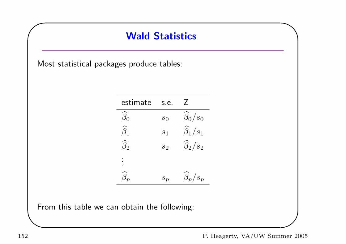
'
&
$
%
Wald Statistics
Most statistical packages produce tables:
estimate s.e. Z
β0 s0 β0/s0
β1 s1 β1/s1
β2 s2 β2/s2
...
βp sp βp/sp
From this table we can obtain the following:
152 P. Heagerty, VA/UW Summer 2005
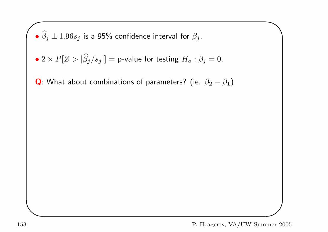
'
&
$
%
• βj ± 1.96sj is a 95% confidence interval for βj .
• 2× P [Z > |βj/sj |] = p-value for testing Ho : βj = 0.
Q: What about combinations of parameters? (ie. β2 − β1)
153 P. Heagerty, VA/UW Summer 2005
'
&
$
%
Multiple Predictors
Example: Remission data
Response = time until death or relapse.
Covariates = treatment group, WBC count.
154 P. Heagerty, VA/UW Summer 2005
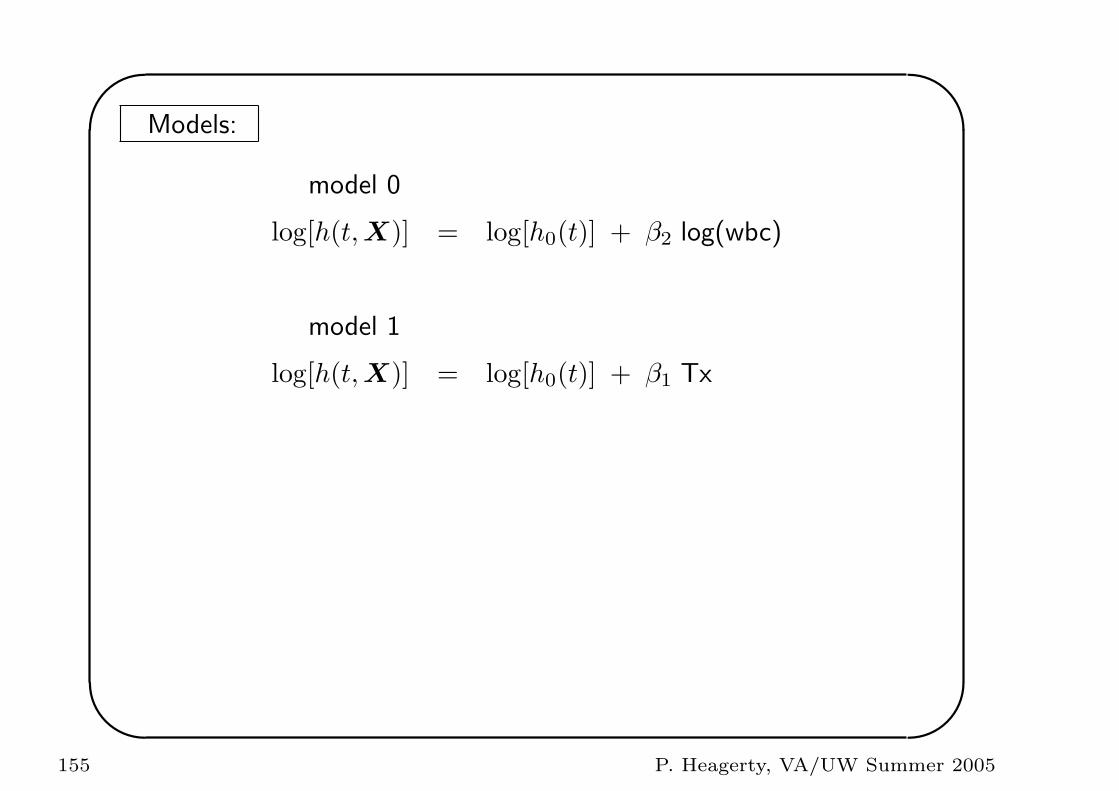
'
&
$
%
Models:
model 0
log[h(t, X)] = log[h0(t)] + β2 log(wbc)
model 1
log[h(t, X)] = log[h0(t)] + β1 Tx
155 P. Heagerty, VA/UW Summer 2005
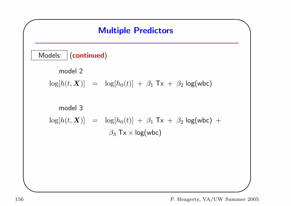
'
&
$
%
Multiple Predictors
Models: (continued)
model 2
log[h(t,X)] = log[h0(t)] + β1 Tx + β2 log(wbc)
model 3
log[h(t,X)] = log[h0(t)] + β1 Tx + β2 log(wbc) +
β3 Tx× log(wbc)
156 P. Heagerty, VA/UW Summer 2005
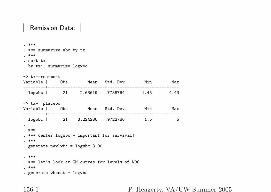
Remission Data:
. ***
. *** summarize wbc by tx
. ***
. sort tx
. by tx: summarize logwbc
-> tx=treatmentVariable | Obs Mean Std. Dev. Min Max---------+-----------------------------------------------------
logwbc | 21 2.63619 .7738764 1.45 4.43
-> tx= placeboVariable | Obs Mean Std. Dev. Min Max---------+-----------------------------------------------------
logwbc | 21 3.224286 .9722786 1.5 5.. ***. *** center logwbc = important for survival!. ***. generate newlwbc = logwbc-3.00
. ***
. *** let’s look at KM curves for levels of WBC
. ***
. generate wbccat = logwbc
156-1 P. Heagerty, VA/UW Summer 2005
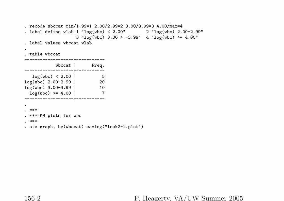
. recode wbccat min/1.99=1 2.00/2.99=2 3.00/3.99=3 4.00/max=4
. label define wlab 1 "log(wbc) < 2.00" 2 "log(wbc) 2.00-2.99"3 "log(wbc) 3.00 > -3.99" 4 "log(wbc) >= 4.00"
. label values wbccat wlab
.
. table wbccat-------------------+-----------
wbccat | Freq.-------------------+-----------
log(wbc) < 2.00 | 5log(wbc) 2.00-2.99 | 20log(wbc) 3.00-3.99 | 10
log(wbc) >= 4.00 | 7-------------------+-----------.. ***. *** KM plots for wbc. ***. sts graph, by(wbccat) saving("leuk2-1.plot")
156-2 P. Heagerty, VA/UW Summer 2005
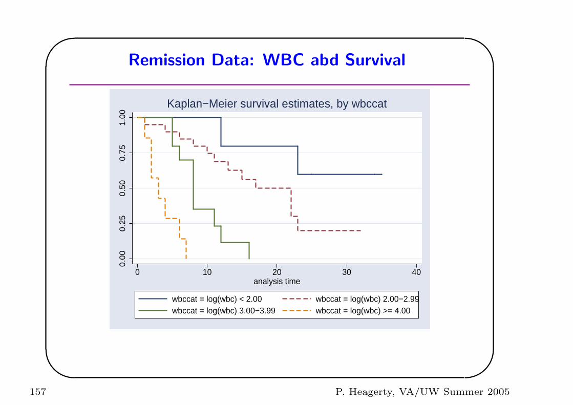
'
&
$
%
Remission Data: WBC abd Survival
0.00
0.25
0.50
0.75
1.00
0 10 20 30 40analysis time
wbccat = log(wbc) < 2.00 wbccat = log(wbc) 2.00−2.99wbccat = log(wbc) 3.00−3.99 wbccat = log(wbc) >= 4.00
Kaplan−Meier survival estimates, by wbccat
157 P. Heagerty, VA/UW Summer 2005
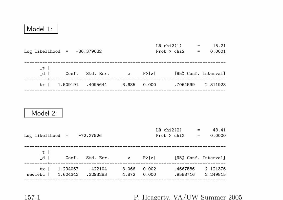
Model 1:
LR chi2(1) = 15.21Log likelihood = -86.379622 Prob > chi2 = 0.0001
------------------------------------------------------------------------------_t |_d | Coef. Std. Err. z P>|z| [95% Conf. Interval]
---------+--------------------------------------------------------------------tx | 1.509191 .4095644 3.685 0.000 .7064599 2.311923
------------------------------------------------------------------------------
Model 2:
LR chi2(2) = 43.41Log likelihood = -72.27926 Prob > chi2 = 0.0000
------------------------------------------------------------------------------_t |_d | Coef. Std. Err. z P>|z| [95% Conf. Interval]
---------+--------------------------------------------------------------------tx | 1.294067 .422104 3.066 0.002 .4667586 2.121376
newlwbc | 1.604343 .3293283 4.872 0.000 .9588716 2.249815------------------------------------------------------------------------------
157-1 P. Heagerty, VA/UW Summer 2005
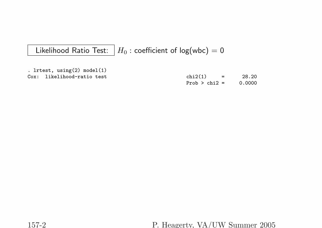
Likelihood Ratio Test: H0 : coefficient of log(wbc) = 0
. lrtest, using(2) model(1)Cox: likelihood-ratio test chi2(1) = 28.20
Prob > chi2 = 0.0000
157-2 P. Heagerty, VA/UW Summer 2005
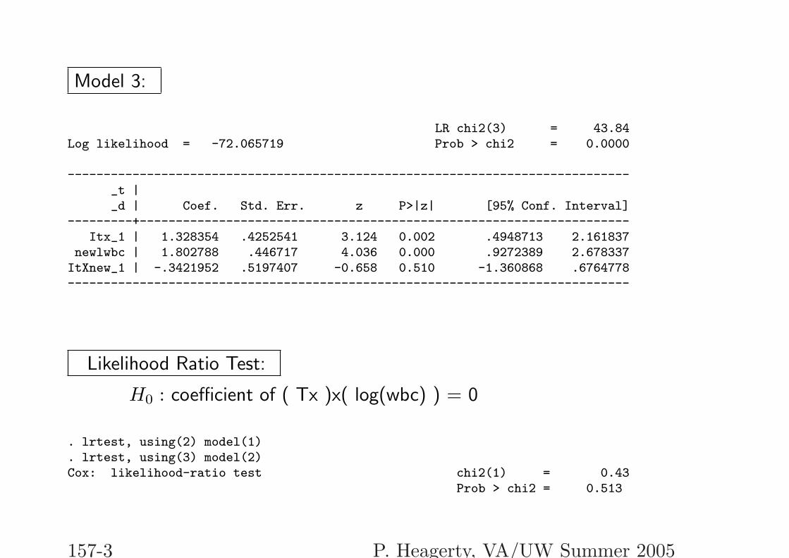
Model 3:
LR chi2(3) = 43.84Log likelihood = -72.065719 Prob > chi2 = 0.0000
------------------------------------------------------------------------------_t |_d | Coef. Std. Err. z P>|z| [95% Conf. Interval]
---------+--------------------------------------------------------------------Itx_1 | 1.328354 .4252541 3.124 0.002 .4948713 2.161837
newlwbc | 1.802788 .446717 4.036 0.000 .9272389 2.678337ItXnew_1 | -.3421952 .5197407 -0.658 0.510 -1.360868 .6764778------------------------------------------------------------------------------
Likelihood Ratio Test:
H0 : coefficient of ( Tx )x( log(wbc) ) = 0
. lrtest, using(2) model(1)
. lrtest, using(3) model(2)Cox: likelihood-ratio test chi2(1) = 0.43
Prob > chi2 = 0.513
157-3 P. Heagerty, VA/UW Summer 2005
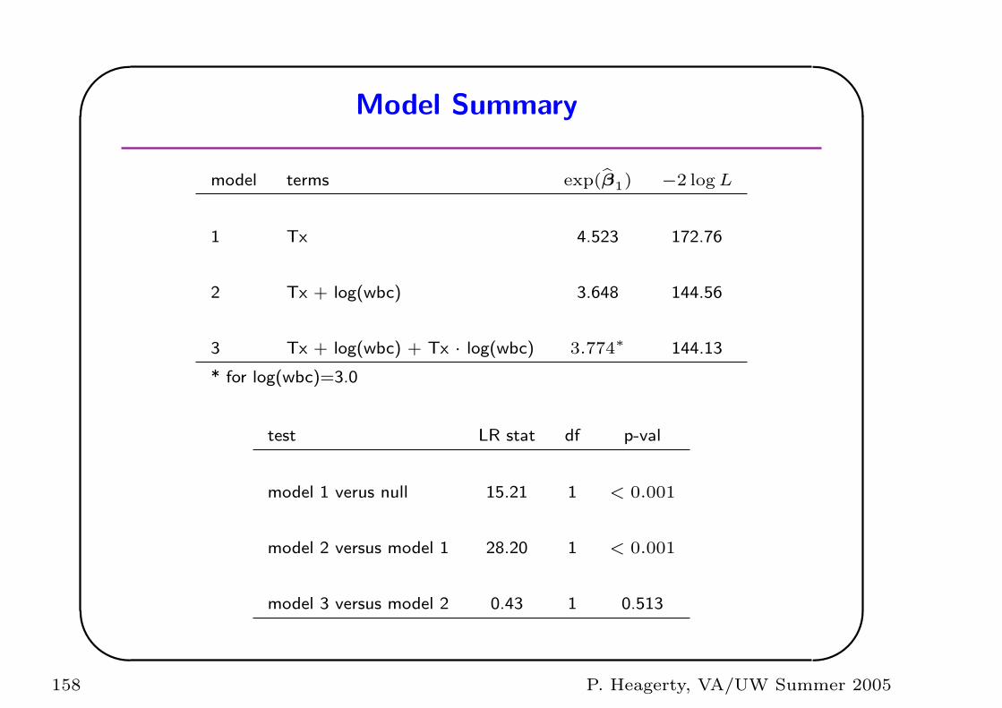
'
&
$
%
Model Summary
model terms exp(β1) −2 log L
1 Tx 4.523 172.76
2 Tx + log(wbc) 3.648 144.56
3 Tx + log(wbc) + Tx · log(wbc) 3.774∗ 144.13
* for log(wbc)=3.0
test LR stat df p-val
model 1 verus null 15.21 1 < 0.001
model 2 versus model 1 28.20 1 < 0.001
model 3 versus model 2 0.43 1 0.513
158 P. Heagerty, VA/UW Summer 2005
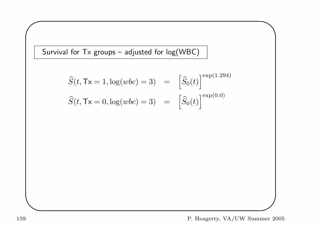
'
&
$
%
Survival for Tx groups – adjusted for log(WBC)
S(t, Tx = 1, log(wbc) = 3) =[S0(t)
]exp(1.294)
S(t, Tx = 0, log(wbc) = 3) =[S0(t)
]exp(0.0)
159 P. Heagerty, VA/UW Summer 2005
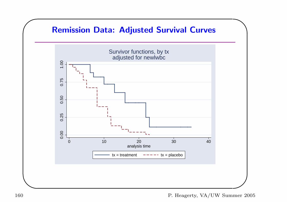
'
&
$
%
Remission Data: Adjusted Survival Curves
0.00
0.25
0.50
0.75
1.00
0 10 20 30 40analysis time
tx = treatment tx = placebo
Survivor functions, by txadjusted for newlwbc
160 P. Heagerty, VA/UW Summer 2005
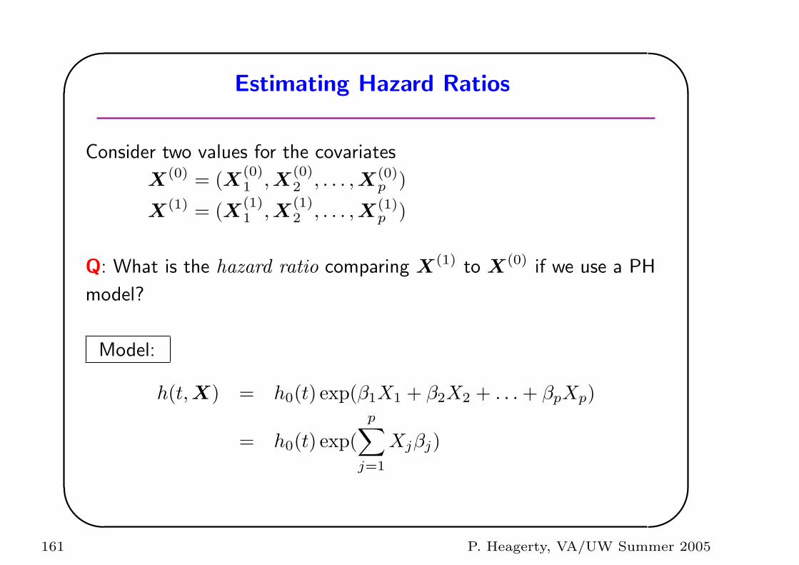
'
&
$
%
Estimating Hazard Ratios
Consider two values for the covariates
X(0) = (X(0)1 , X
(0)2 , . . . , X(0)
p )
X(1) = (X(1)1 , X
(1)2 , . . . , X(1)
p )
Q: What is the hazard ratio comparing X(1) to X(0) if we use a PH
model?
Model:
h(t,X) = h0(t) exp(β1X1 + β2X2 + . . . + βpXp)
= h0(t) exp(p∑
j=1
Xjβj)
161 P. Heagerty, VA/UW Summer 2005
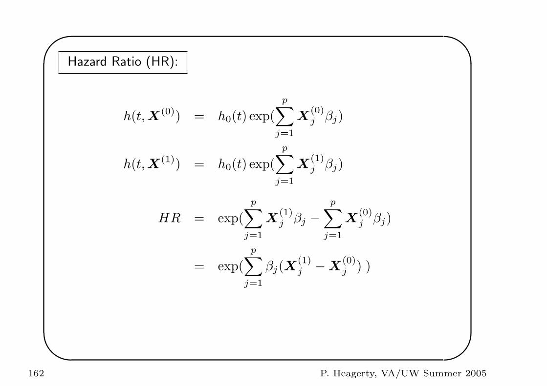
'
&
$
%
Hazard Ratio (HR):
h(t,X(0)) = h0(t) exp(p∑
j=1
X(0)j βj)
h(t,X(1)) = h0(t) exp(p∑
j=1
X(1)j βj)
HR = exp(p∑
j=1
X(1)j βj −
p∑
j=1
X(0)j βj)
= exp(p∑
j=1
βj(X(1)j −X
(0)j ) )
162 P. Heagerty, VA/UW Summer 2005
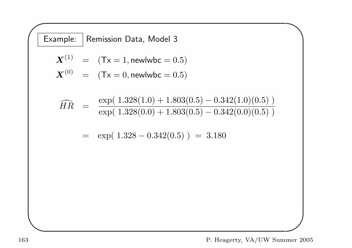
'
&
$
%
Example: Remission Data, Model 3
X(1) = (Tx = 1, newlwbc = 0.5)
X(0) = (Tx = 0, newlwbc = 0.5)
HR =exp( 1.328(1.0) + 1.803(0.5)− 0.342(1.0)(0.5) )exp( 1.328(0.0) + 1.803(0.5)− 0.342(0.0)(0.5) )
= exp( 1.328− 0.342(0.5) ) = 3.180
163 P. Heagerty, VA/UW Summer 2005
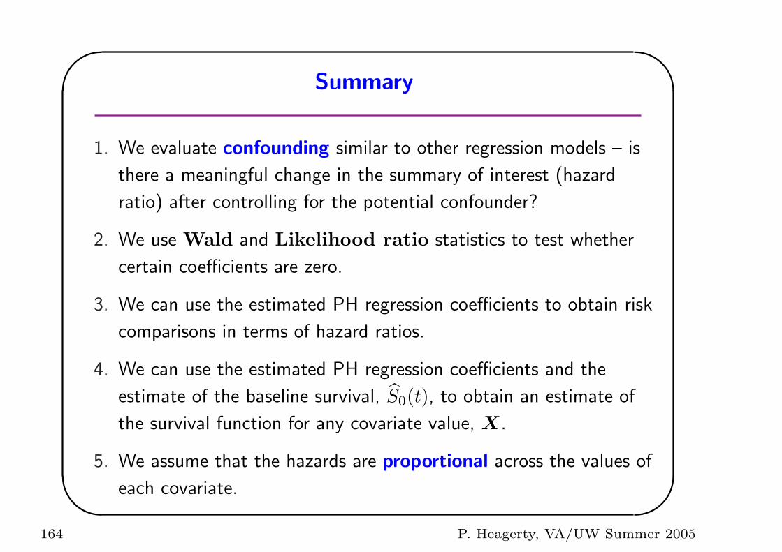
'
&
$
%
Summary
1. We evaluate confounding similar to other regression models – is
there a meaningful change in the summary of interest (hazard
ratio) after controlling for the potential confounder?
2. We use Wald and Likelihood ratio statistics to test whether
certain coefficients are zero.
3. We can use the estimated PH regression coefficients to obtain risk
comparisons in terms of hazard ratios.
4. We can use the estimated PH regression coefficients and the
estimate of the baseline survival, S0(t), to obtain an estimate of
the survival function for any covariate value, X.
5. We assume that the hazards are proportional across the values of
each covariate.
164 P. Heagerty, VA/UW Summer 2005
'
&
$
%
6. We assume that the comparison of hazards for X = 1 versus
X = 0 does not depend on the time, t.
7. Q: How can we check the PH assumption?
165 P. Heagerty, VA/UW Summer 2005
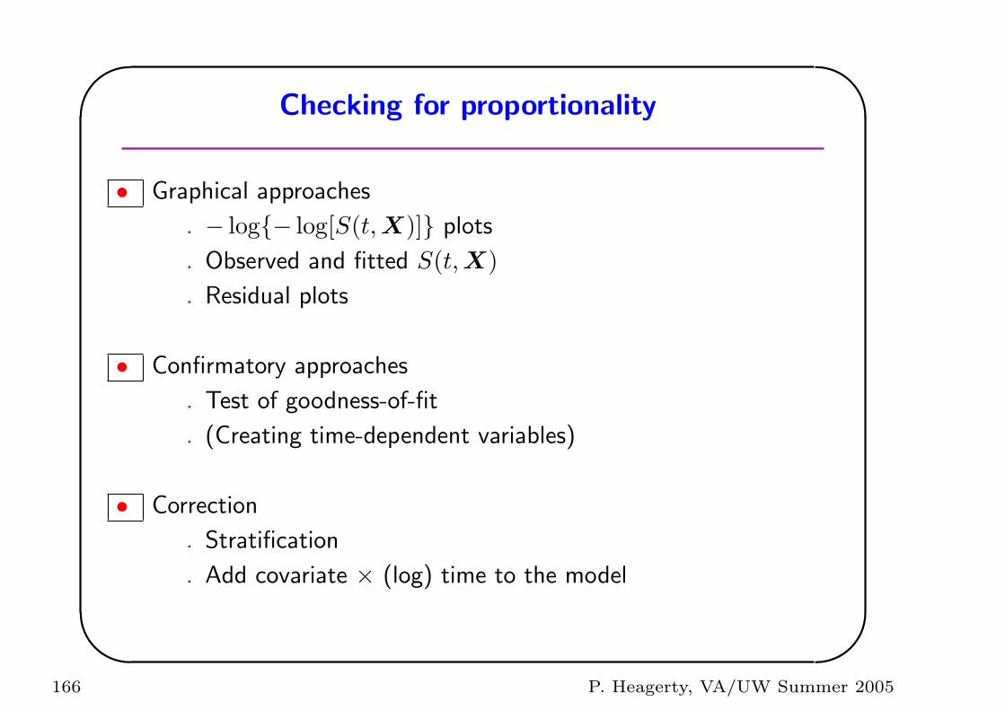
'
&
$
%
Checking for proportionality
• Graphical approaches
. − log{− log[S(t,X)]} plots
. Observed and fitted S(t,X)
. Residual plots
• Confirmatory approaches
. Test of goodness-of-fit
. (Creating time-dependent variables)
• Correction
. Stratification
. Add covariate × (log) time to the model
166 P. Heagerty, VA/UW Summer 2005
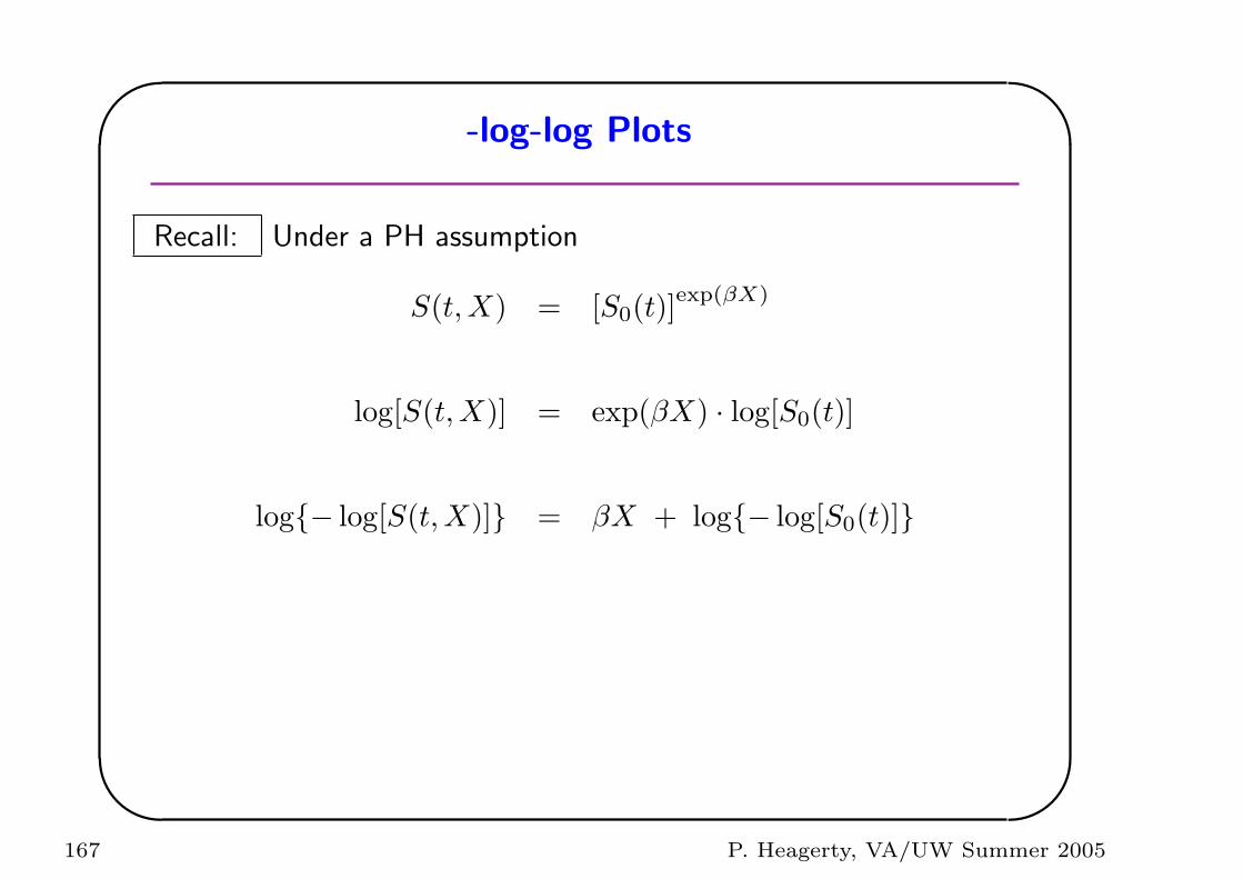
'
&
$
%
-log-log Plots
Recall: Under a PH assumption
S(t,X) = [S0(t)]exp(βX)
log[S(t,X)] = exp(βX) · log[S0(t)]
log{− log[S(t,X)]} = βX + log{− log[S0(t)]}
167 P. Heagerty, VA/UW Summer 2005
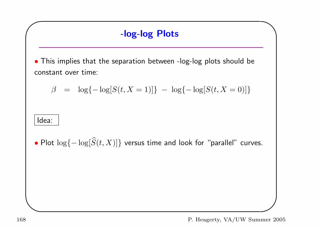
'
&
$
%
-log-log Plots
• This implies that the separation between -log-log plots should be
constant over time:
β = log{− log[S(t,X = 1)]} − log{− log[S(t,X = 0)]}
Idea:
• Plot log{− log[S(t,X)]} versus time and look for “parallel” curves.
168 P. Heagerty, VA/UW Summer 2005
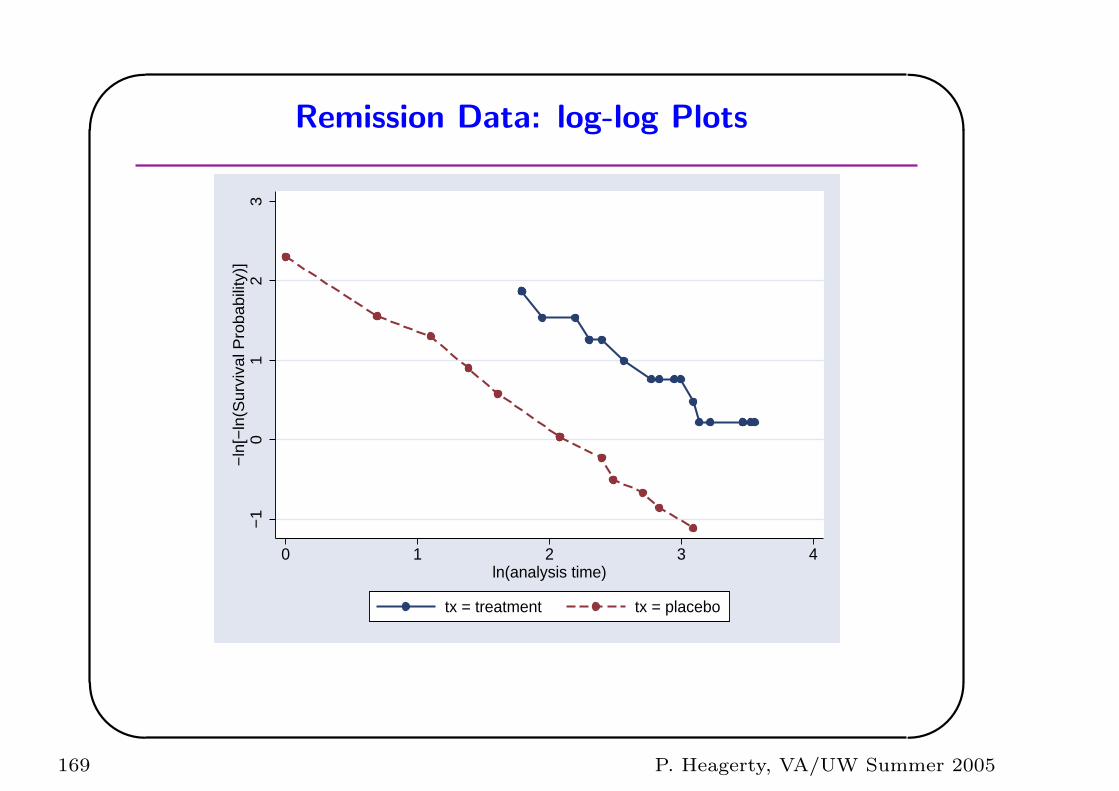
'
&
$
%
Remission Data: log-log Plots
−1
01
23
−ln
[−ln
(Sur
viva
l Pro
babi
lity)
]
0 1 2 3 4ln(analysis time)
tx = treatment tx = placebo
169 P. Heagerty, VA/UW Summer 2005
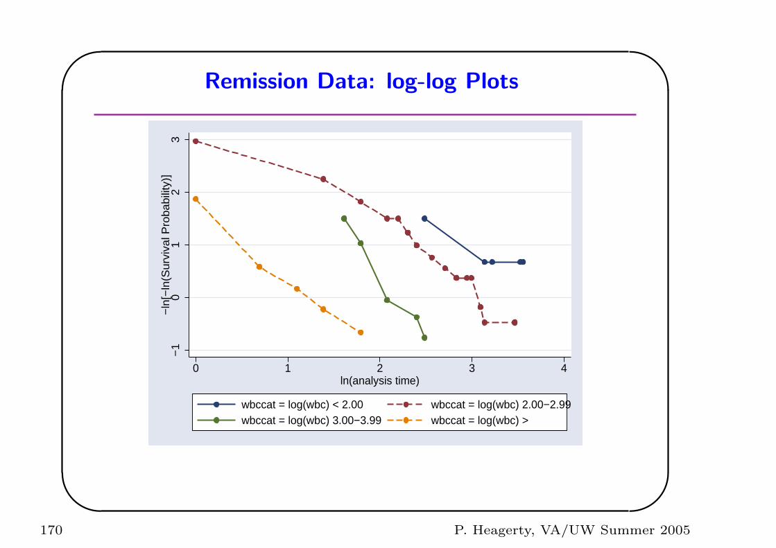
'
&
$
%
Remission Data: log-log Plots
−1
01
23
−ln
[−ln
(Sur
viva
l Pro
babi
lity)
]
0 1 2 3 4ln(analysis time)
wbccat = log(wbc) < 2.00 wbccat = log(wbc) 2.00−2.99wbccat = log(wbc) 3.00−3.99 wbccat = log(wbc) >
170 P. Heagerty, VA/UW Summer 2005
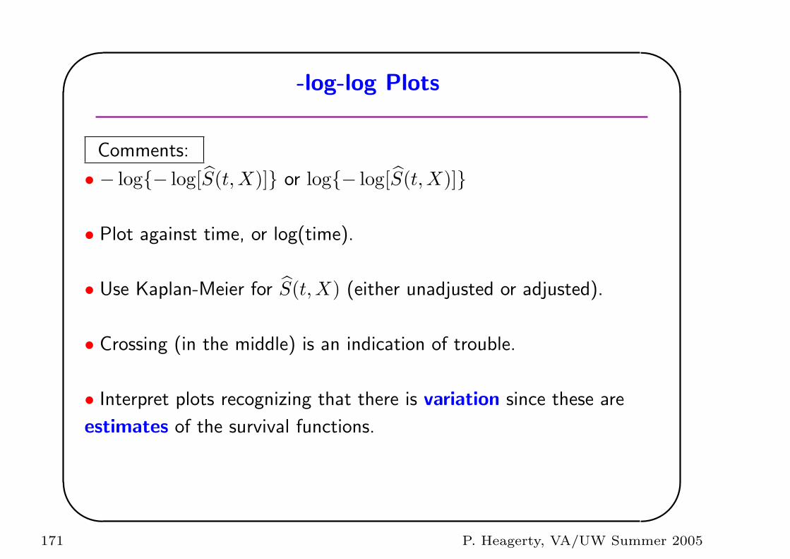
'
&
$
%
-log-log Plots
Comments:
• − log{− log[S(t,X)]} or log{− log[S(t,X)]}
• Plot against time, or log(time).
• Use Kaplan-Meier for S(t,X) (either unadjusted or adjusted).
• Crossing (in the middle) is an indication of trouble.
• Interpret plots recognizing that there is variation since these are
estimates of the survival functions.
171 P. Heagerty, VA/UW Summer 2005
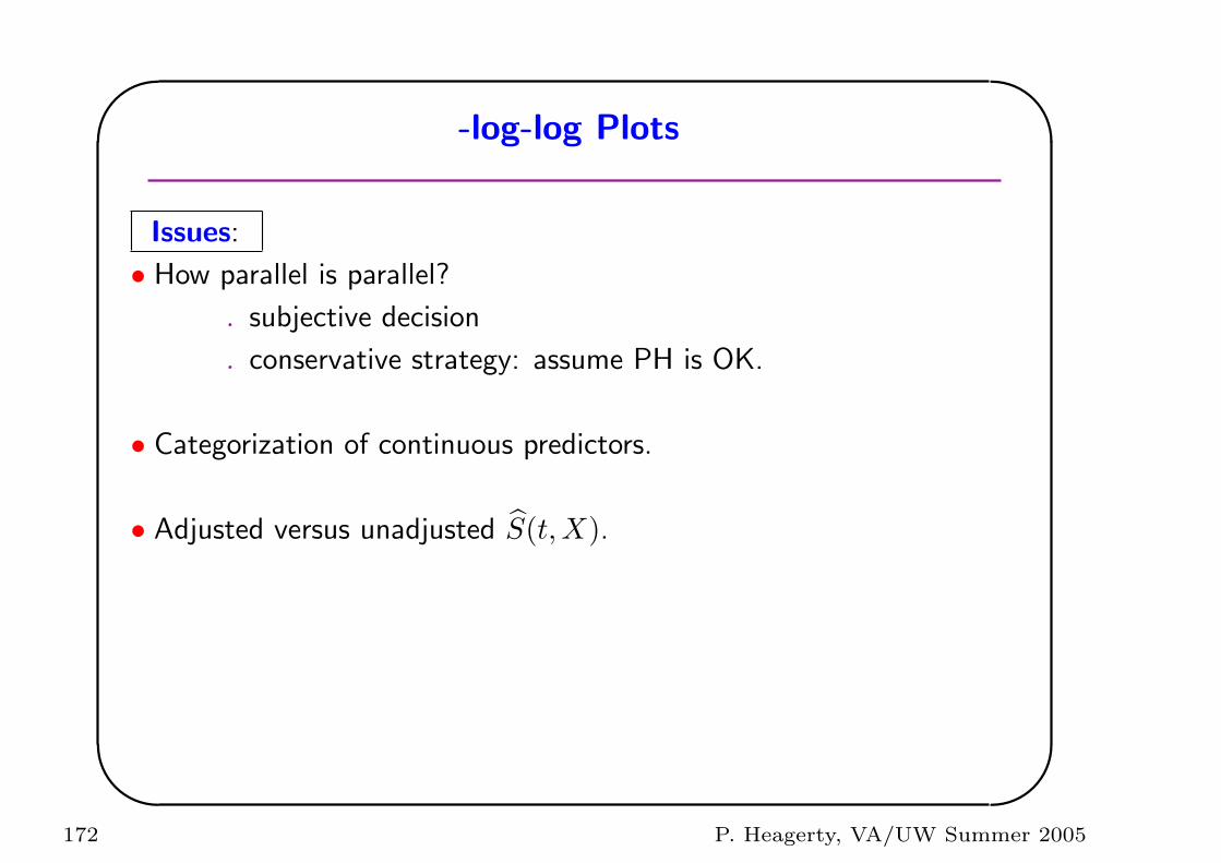
'
&
$
%
-log-log Plots
Issues:
• How parallel is parallel?
. subjective decision
. conservative strategy: assume PH is OK.
• Categorization of continuous predictors.
• Adjusted versus unadjusted S(t,X).
172 P. Heagerty, VA/UW Summer 2005
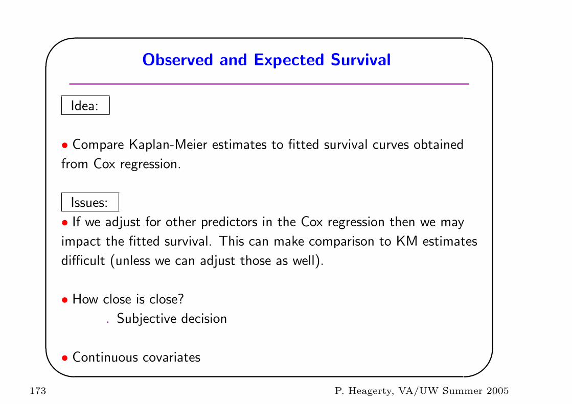
'
&
$
%
Observed and Expected Survival
Idea:
• Compare Kaplan-Meier estimates to fitted survival curves obtained
from Cox regression.
Issues:
• If we adjust for other predictors in the Cox regression then we may
impact the fitted survival. This can make comparison to KM estimates
difficult (unless we can adjust those as well).
• How close is close?
. Subjective decision
• Continuous covariates
173 P. Heagerty, VA/UW Summer 2005
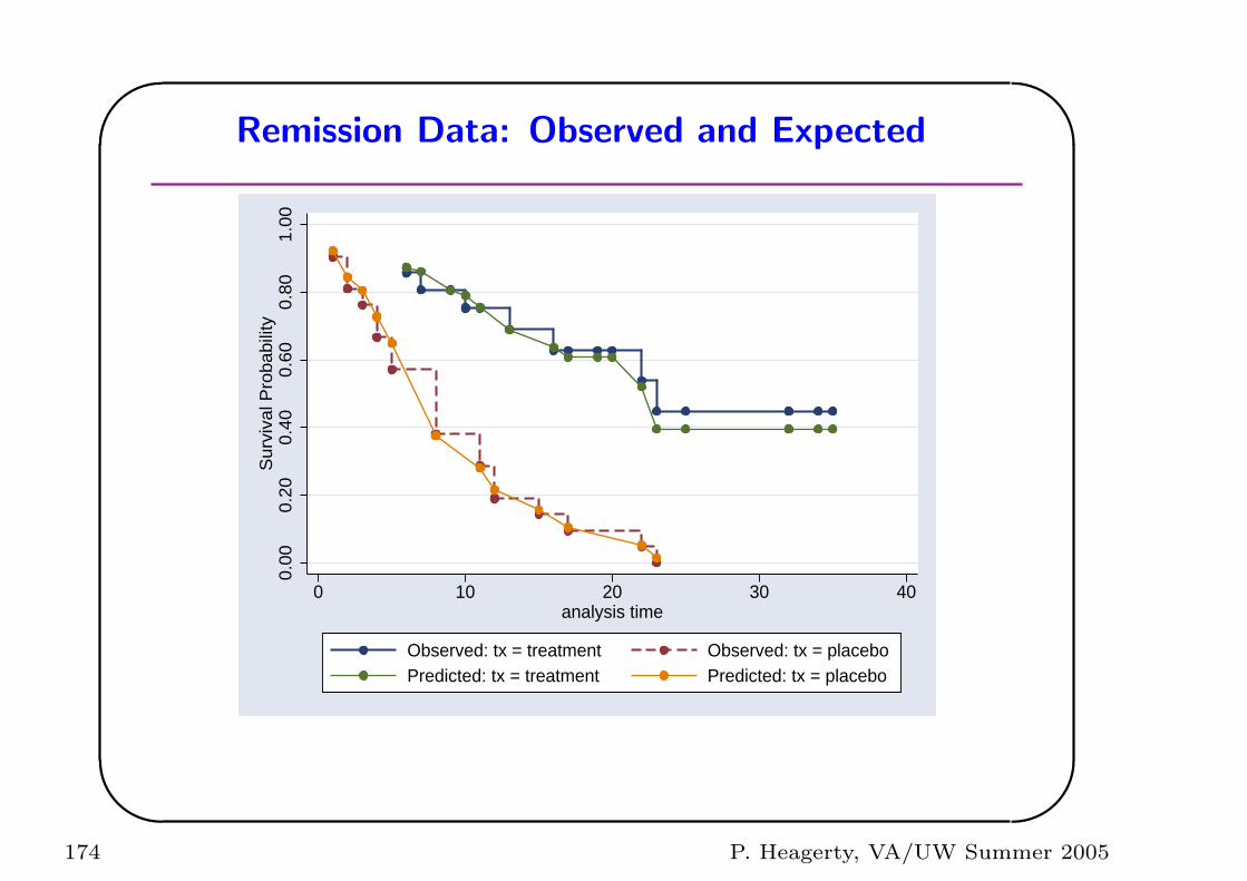
'
&
$
%
Remission Data: Observed and Expected
0.00
0.20
0.40
0.60
0.80
1.00
Sur
viva
l Pro
babi
lity
0 10 20 30 40analysis time
Observed: tx = treatment Observed: tx = placeboPredicted: tx = treatment Predicted: tx = placebo
174 P. Heagerty, VA/UW Summer 2005
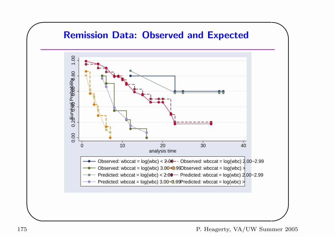
'
&
$
%
Remission Data: Observed and Expected
0.00
0.20
0.40
0.60
0.80
1.00
Sur
viva
l Pro
babi
lity
0 10 20 30 40analysis time
Observed: wbccat = log(wbc) < 2.00 Observed: wbccat = log(wbc) 2.00−2.99Observed: wbccat = log(wbc) 3.00−3.99Observed: wbccat = log(wbc) >Predicted: wbccat = log(wbc) < 2.00 Predicted: wbccat = log(wbc) 2.00−2.99Predicted: wbccat = log(wbc) 3.00−3.99Predicted: wbccat = log(wbc) >
175 P. Heagerty, VA/UW Summer 2005
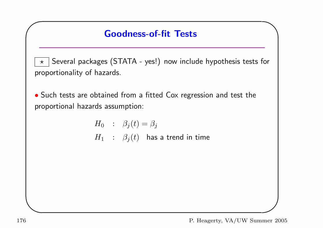
'
&
$
%
Goodness-of-fit Tests
? Several packages (STATA - yes!) now include hypothesis tests for
proportionality of hazards.
• Such tests are obtained from a fitted Cox regression and test the
proportional hazards assumption:
H0 : βj(t) = βj
H1 : βj(t) has a trend in time
176 P. Heagerty, VA/UW Summer 2005
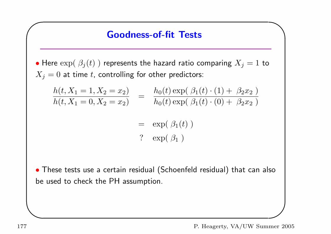
'
&
$
%
Goodness-of-fit Tests
• Here exp( βj(t) ) represents the hazard ratio comparing Xj = 1 to
Xj = 0 at time t, controlling for other predictors:
h(t,X1 = 1, X2 = x2)h(t,X1 = 0, X2 = x2)
=h0(t) exp( β1(t) · (1) + β2x2 )h0(t) exp( β1(t) · (0) + β2x2 )
= exp( β1(t) )
? exp( β1 )
• These tests use a certain residual (Schoenfeld residual) that can also
be used to check the PH assumption.
177 P. Heagerty, VA/UW Summer 2005
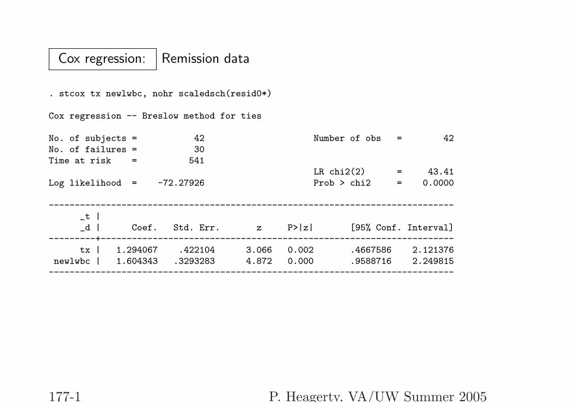
Cox regression: Remission data
. stcox tx newlwbc, nohr scaledsch(resid0*)
Cox regression -- Breslow method for ties
No. of subjects = 42 Number of obs = 42No. of failures = 30Time at risk = 541
LR chi2(2) = 43.41Log likelihood = -72.27926 Prob > chi2 = 0.0000
------------------------------------------------------------------------------_t |_d | Coef. Std. Err. z P>|z| [95% Conf. Interval]
---------+--------------------------------------------------------------------tx | 1.294067 .422104 3.066 0.002 .4667586 2.121376
newlwbc | 1.604343 .3293283 4.872 0.000 .9588716 2.249815------------------------------------------------------------------------------
177-1 P. Heagerty, VA/UW Summer 2005
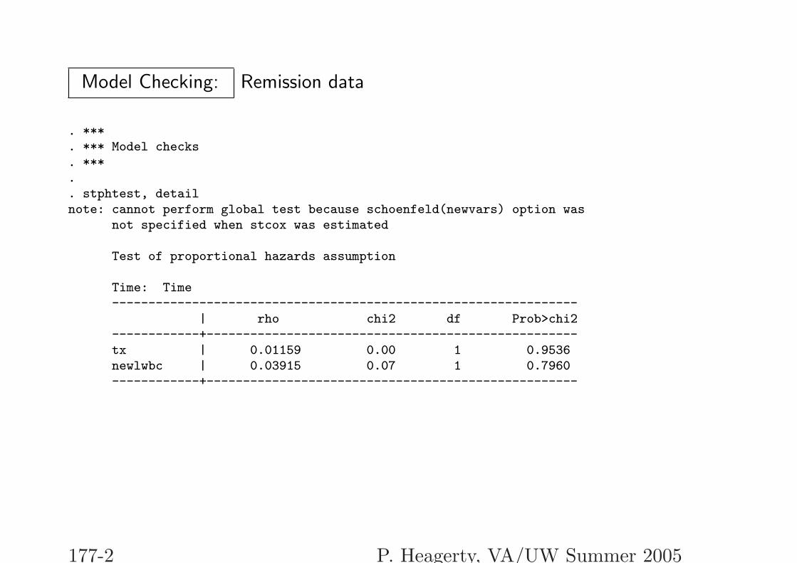
Model Checking: Remission data
. ***
. *** Model checks
. ***
.
. stphtest, detailnote: cannot perform global test because schoenfeld(newvars) option was
not specified when stcox was estimated
Test of proportional hazards assumption
Time: Time----------------------------------------------------------------
| rho chi2 df Prob>chi2------------+---------------------------------------------------tx | 0.01159 0.00 1 0.9536newlwbc | 0.03915 0.07 1 0.7960------------+---------------------------------------------------
177-2 P. Heagerty, VA/UW Summer 2005
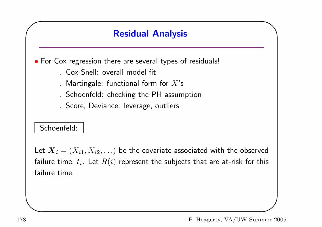
'
&
$
%
Residual Analysis
• For Cox regression there are several types of residuals!
. Cox-Snell: overall model fit
. Martingale: functional form for X’s
. Schoenfeld: checking the PH assumption
. Score, Deviance: leverage, outliers
Schoenfeld:
Let Xi = (Xi1, Xi2, . . .) be the covariate associated with the observed
failure time, ti. Let R(i) represent the subjects that are at-risk for this
failure time.
178 P. Heagerty, VA/UW Summer 2005
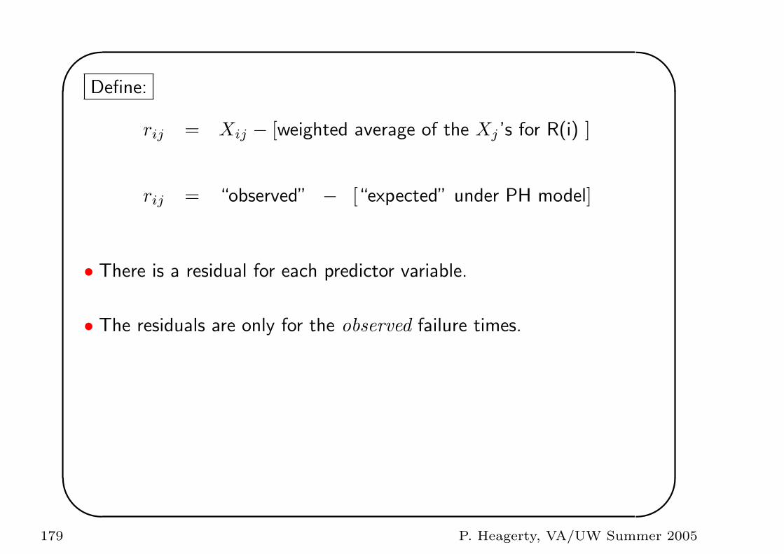
'
&
$
%
Define:
rij = Xij − [weighted average of the Xj ’s for R(i) ]
rij = “observed” − [“expected” under PH model]
• There is a residual for each predictor variable.
• The residuals are only for the observed failure times.
179 P. Heagerty, VA/UW Summer 2005
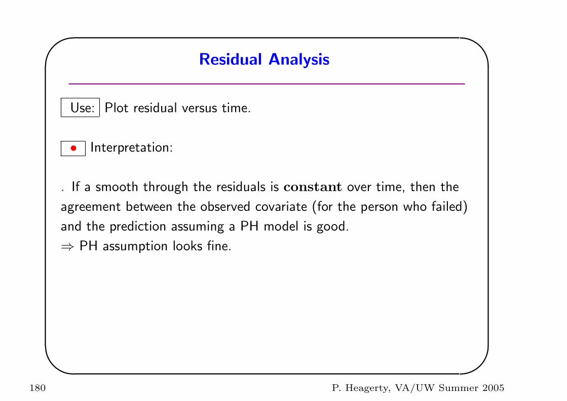
'
&
$
%
Residual Analysis
Use: Plot residual versus time.
• Interpretation:
. If a smooth through the residuals is constant over time, then the
agreement between the observed covariate (for the person who failed)
and the prediction assuming a PH model is good.
⇒ PH assumption looks fine.
180 P. Heagerty, VA/UW Summer 2005
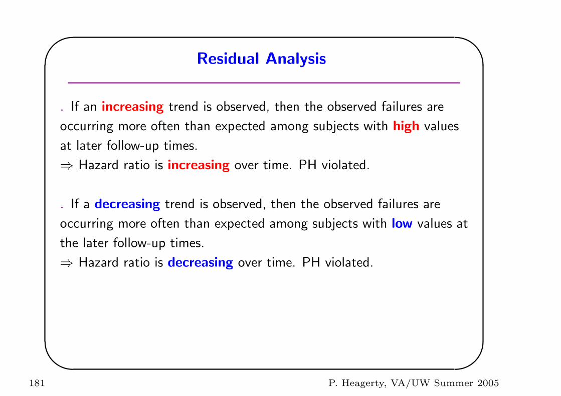
'
&
$
%
Residual Analysis
. If an increasing trend is observed, then the observed failures are
occurring more often than expected among subjects with high values
at later follow-up times.
⇒ Hazard ratio is increasing over time. PH violated.
. If a decreasing trend is observed, then the observed failures are
occurring more often than expected among subjects with low values at
the later follow-up times.
⇒ Hazard ratio is decreasing over time. PH violated.
181 P. Heagerty, VA/UW Summer 2005
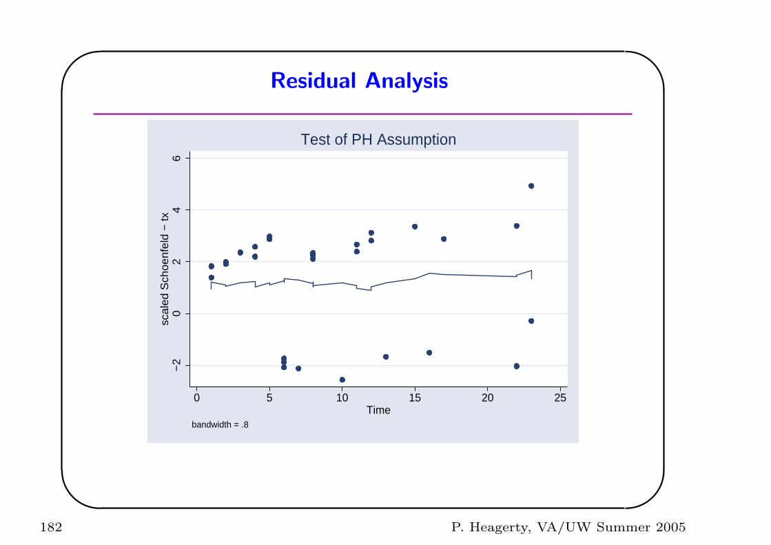
'
&
$
%
Residual Analysis
−2
02
46
scal
ed S
choe
nfel
d −
tx
0 5 10 15 20 25Time
bandwidth = .8
Test of PH Assumption
182 P. Heagerty, VA/UW Summer 2005
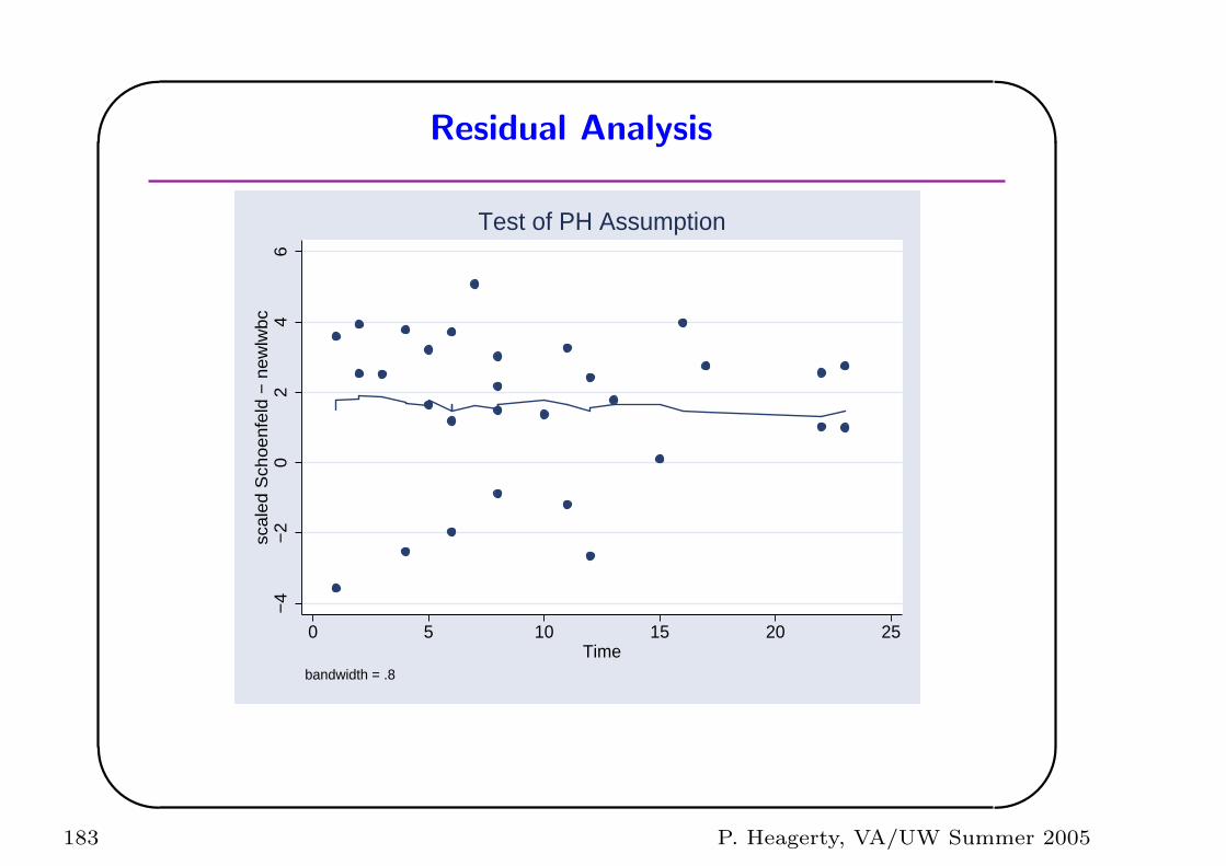
'
&
$
%
Residual Analysis
−4
−2
02
46
scal
ed S
choe
nfel
d −
new
lwbc
0 5 10 15 20 25Time
bandwidth = .8
Test of PH Assumption
183 P. Heagerty, VA/UW Summer 2005
'
&
$
%
Example: Methadone Treatment
• The following analysis considers a dataset from a study by
Caplehorn et al. (“Methadone Dosage and Retention of Patients
in Maintenance Treatment”, Med. J. Aust., 1991). These data
record the time in days spent by heroin addicts from entry to
departure from one of two methadone clinics. There are two
additional covariates, namely, prison record and maximummethadone dose, both believed to correlate with the time spent in
the clinic.
• Objectives:
. Describe the relationship between the covariates and time until
clinic discharge.
. Is prison an important predictor?
. Is dose an important predictor?
184 P. Heagerty, VA/UW Summer 2005
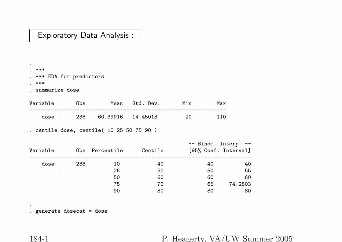
Exploratory Data Analysis :
.
. ***
. *** EDA for predictors
. ***
. summarize dose
Variable | Obs Mean Std. Dev. Min Max---------+-----------------------------------------------------
dose | 238 60.39916 14.45013 20 110
. centile dose, centile( 10 25 50 75 90 )
-- Binom. Interp. --Variable | Obs Percentile Centile [95% Conf. Interval]---------+-------------------------------------------------------------
dose | 238 10 40 40 40| 25 50 50 55| 50 60 60 60| 75 70 65 74.2803| 90 80 80 80
.
. generate dosecat = dose
184-1 P. Heagerty, VA/UW Summer 2005
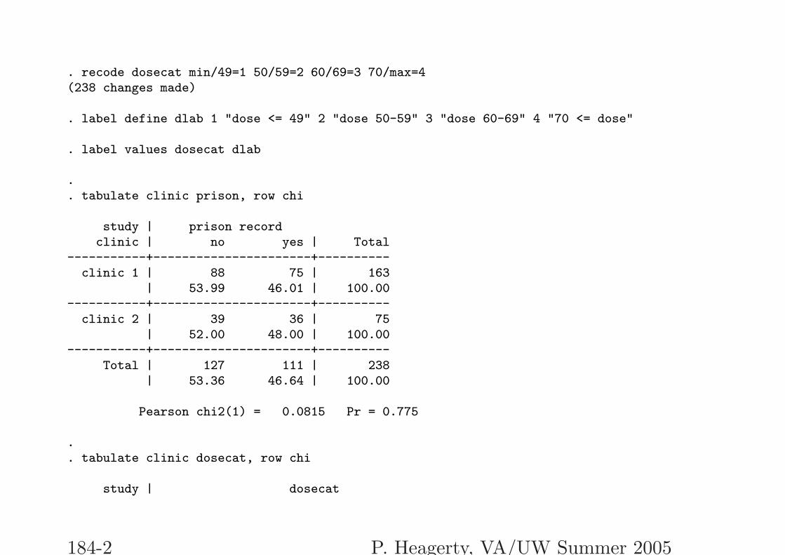
. recode dosecat min/49=1 50/59=2 60/69=3 70/max=4(238 changes made)
. label define dlab 1 "dose <= 49" 2 "dose 50-59" 3 "dose 60-69" 4 "70 <= dose"
. label values dosecat dlab
.
. tabulate clinic prison, row chi
study | prison recordclinic | no yes | Total
-----------+----------------------+----------clinic 1 | 88 75 | 163
| 53.99 46.01 | 100.00-----------+----------------------+----------
clinic 2 | 39 36 | 75| 52.00 48.00 | 100.00
-----------+----------------------+----------Total | 127 111 | 238
| 53.36 46.64 | 100.00
Pearson chi2(1) = 0.0815 Pr = 0.775
.
. tabulate clinic dosecat, row chi
study | dosecat
184-2 P. Heagerty, VA/UW Summer 2005
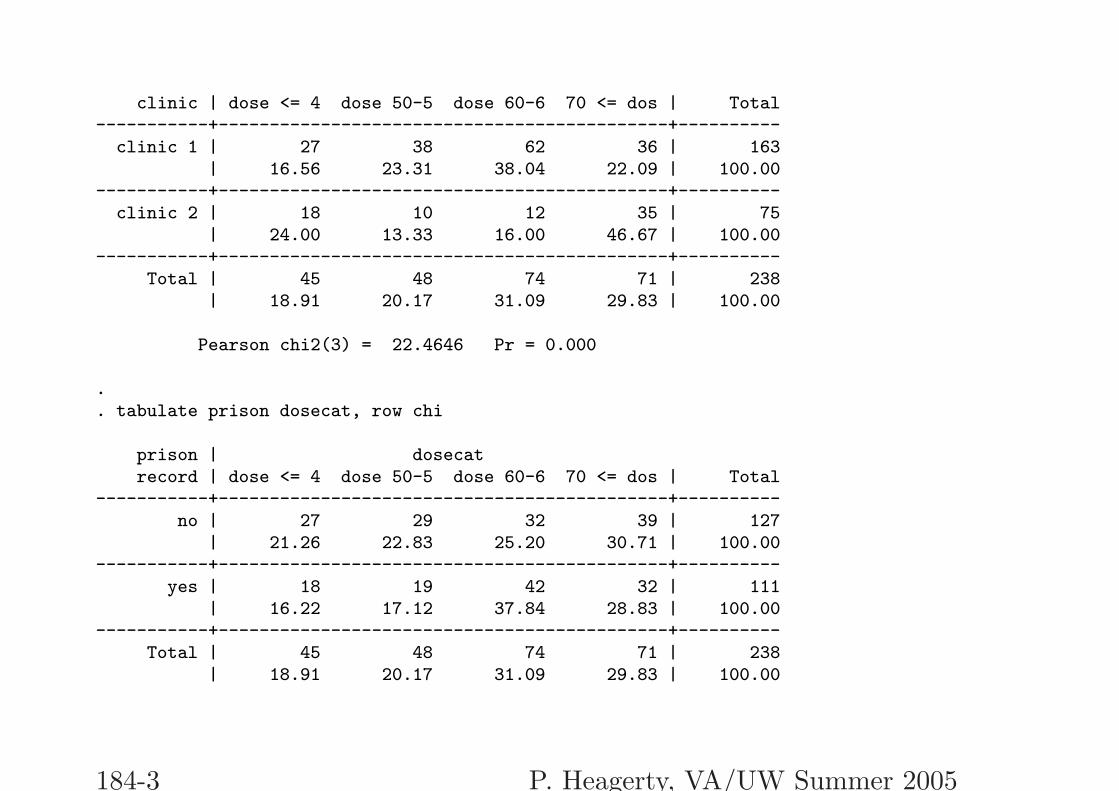
clinic | dose <= 4 dose 50-5 dose 60-6 70 <= dos | Total-----------+--------------------------------------------+----------
clinic 1 | 27 38 62 36 | 163| 16.56 23.31 38.04 22.09 | 100.00
-----------+--------------------------------------------+----------clinic 2 | 18 10 12 35 | 75
| 24.00 13.33 16.00 46.67 | 100.00-----------+--------------------------------------------+----------
Total | 45 48 74 71 | 238| 18.91 20.17 31.09 29.83 | 100.00
Pearson chi2(3) = 22.4646 Pr = 0.000
.
. tabulate prison dosecat, row chi
prison | dosecatrecord | dose <= 4 dose 50-5 dose 60-6 70 <= dos | Total
-----------+--------------------------------------------+----------no | 27 29 32 39 | 127
| 21.26 22.83 25.20 30.71 | 100.00-----------+--------------------------------------------+----------
yes | 18 19 42 32 | 111| 16.22 17.12 37.84 28.83 | 100.00
-----------+--------------------------------------------+----------Total | 45 48 74 71 | 238
| 18.91 20.17 31.09 29.83 | 100.00
184-3 P. Heagerty, VA/UW Summer 2005
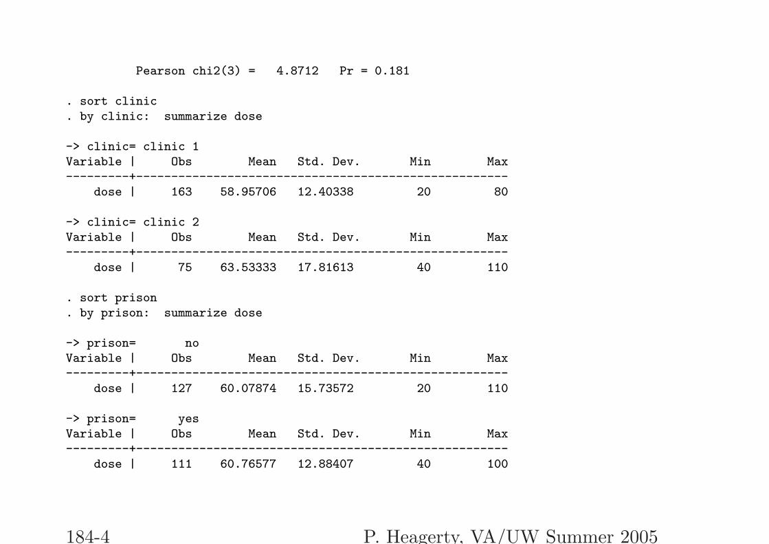
Pearson chi2(3) = 4.8712 Pr = 0.181
. sort clinic
. by clinic: summarize dose
-> clinic= clinic 1Variable | Obs Mean Std. Dev. Min Max---------+-----------------------------------------------------
dose | 163 58.95706 12.40338 20 80
-> clinic= clinic 2Variable | Obs Mean Std. Dev. Min Max---------+-----------------------------------------------------
dose | 75 63.53333 17.81613 40 110
. sort prison
. by prison: summarize dose
-> prison= noVariable | Obs Mean Std. Dev. Min Max---------+-----------------------------------------------------
dose | 127 60.07874 15.73572 20 110
-> prison= yesVariable | Obs Mean Std. Dev. Min Max---------+-----------------------------------------------------
dose | 111 60.76577 12.88407 40 100
184-4 P. Heagerty, VA/UW Summer 2005
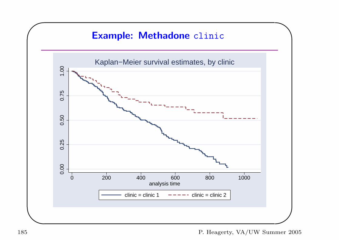
'
&
$
%
Example: Methadone clinic
0.00
0.25
0.50
0.75
1.00
0 200 400 600 800 1000analysis time
clinic = clinic 1 clinic = clinic 2
Kaplan−Meier survival estimates, by clinic
185 P. Heagerty, VA/UW Summer 2005
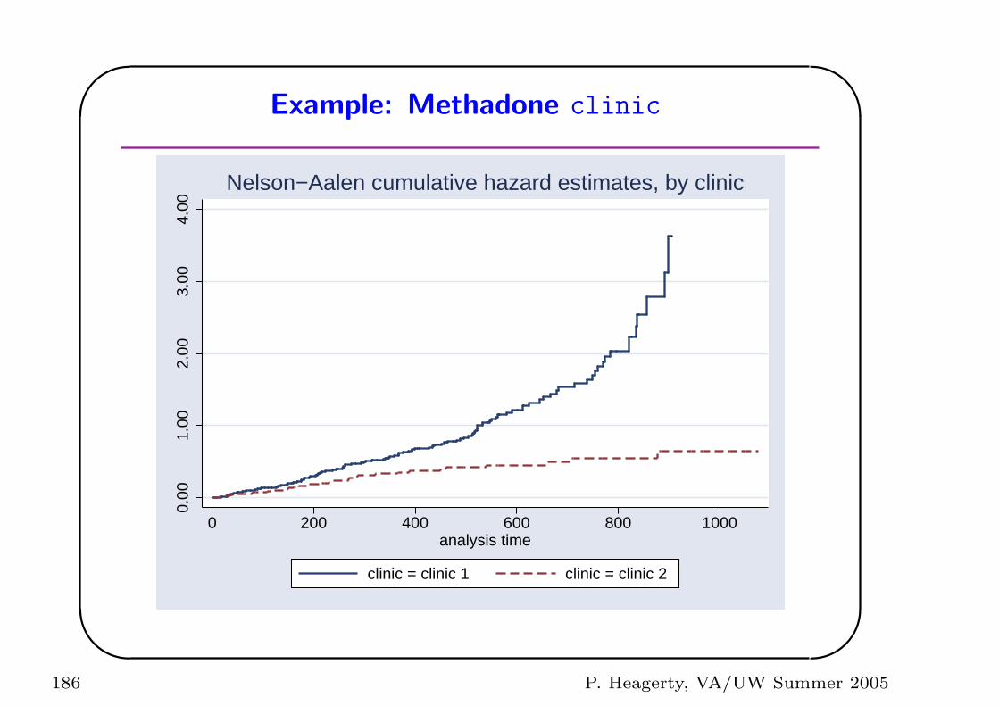
'
&
$
%
Example: Methadone clinic
0.00
1.00
2.00
3.00
4.00
0 200 400 600 800 1000analysis time
clinic = clinic 1 clinic = clinic 2
Nelson−Aalen cumulative hazard estimates, by clinic
186 P. Heagerty, VA/UW Summer 2005
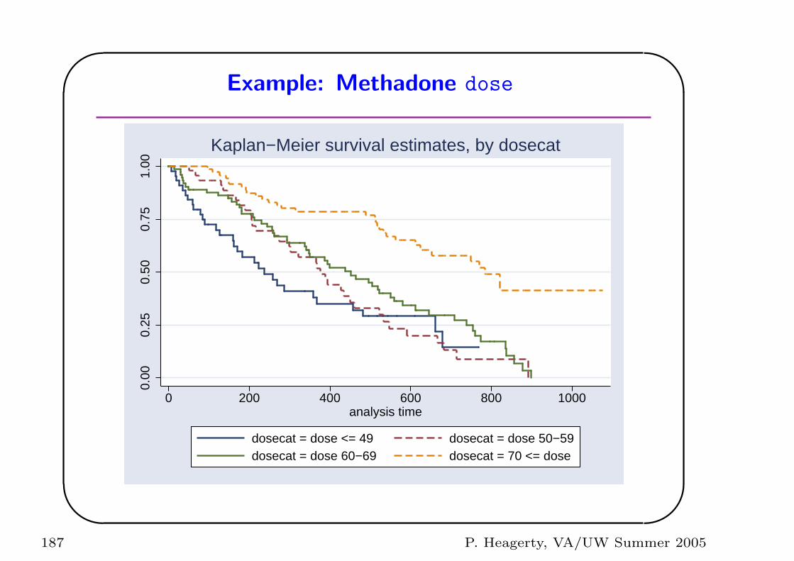
'
&
$
%
Example: Methadone dose
0.00
0.25
0.50
0.75
1.00
0 200 400 600 800 1000analysis time
dosecat = dose <= 49 dosecat = dose 50−59dosecat = dose 60−69 dosecat = 70 <= dose
Kaplan−Meier survival estimates, by dosecat
187 P. Heagerty, VA/UW Summer 2005
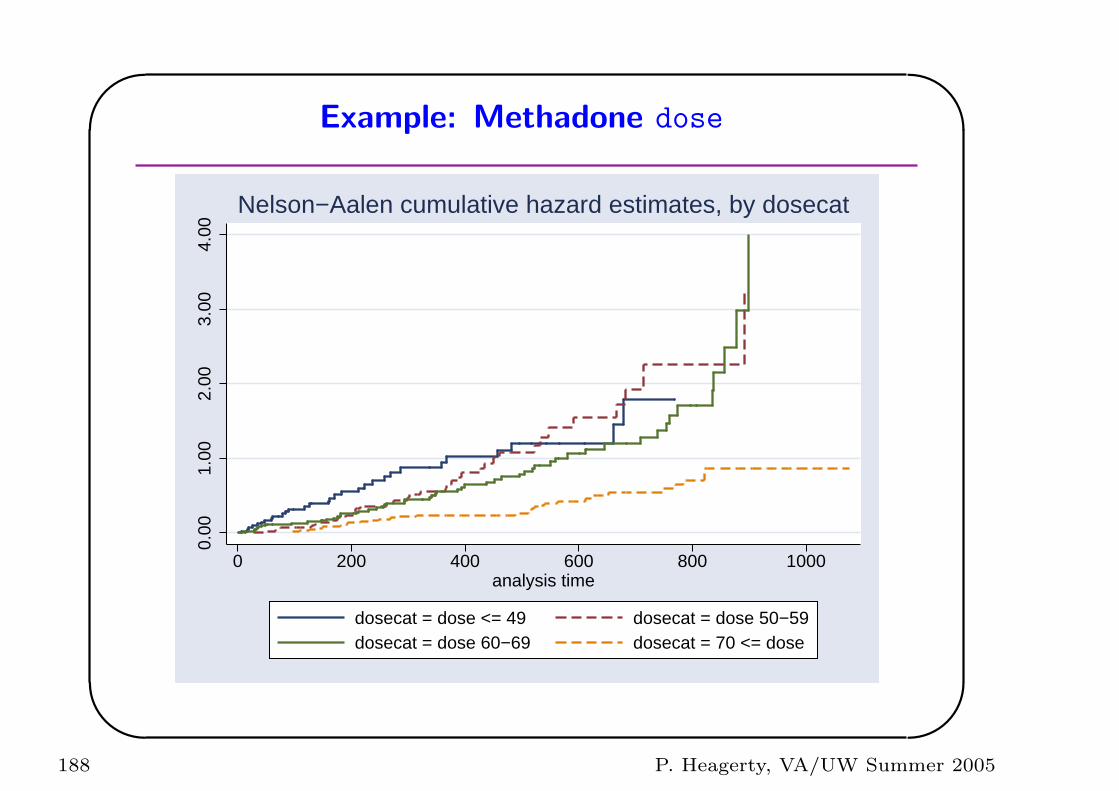
'
&
$
%
Example: Methadone dose
0.00
1.00
2.00
3.00
4.00
0 200 400 600 800 1000analysis time
dosecat = dose <= 49 dosecat = dose 50−59dosecat = dose 60−69 dosecat = 70 <= dose
Nelson−Aalen cumulative hazard estimates, by dosecat
188 P. Heagerty, VA/UW Summer 2005
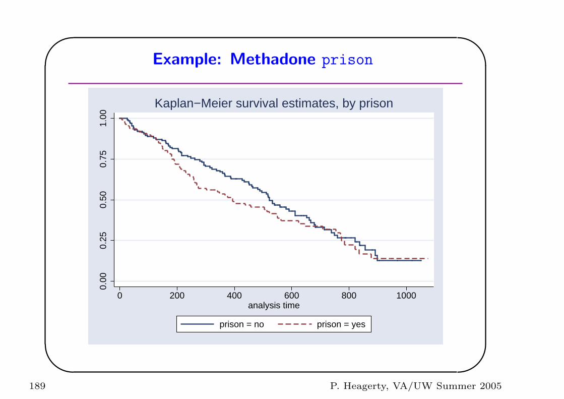
'
&
$
%
Example: Methadone prison
0.00
0.25
0.50
0.75
1.00
0 200 400 600 800 1000analysis time
prison = no prison = yes
Kaplan−Meier survival estimates, by prison
189 P. Heagerty, VA/UW Summer 2005
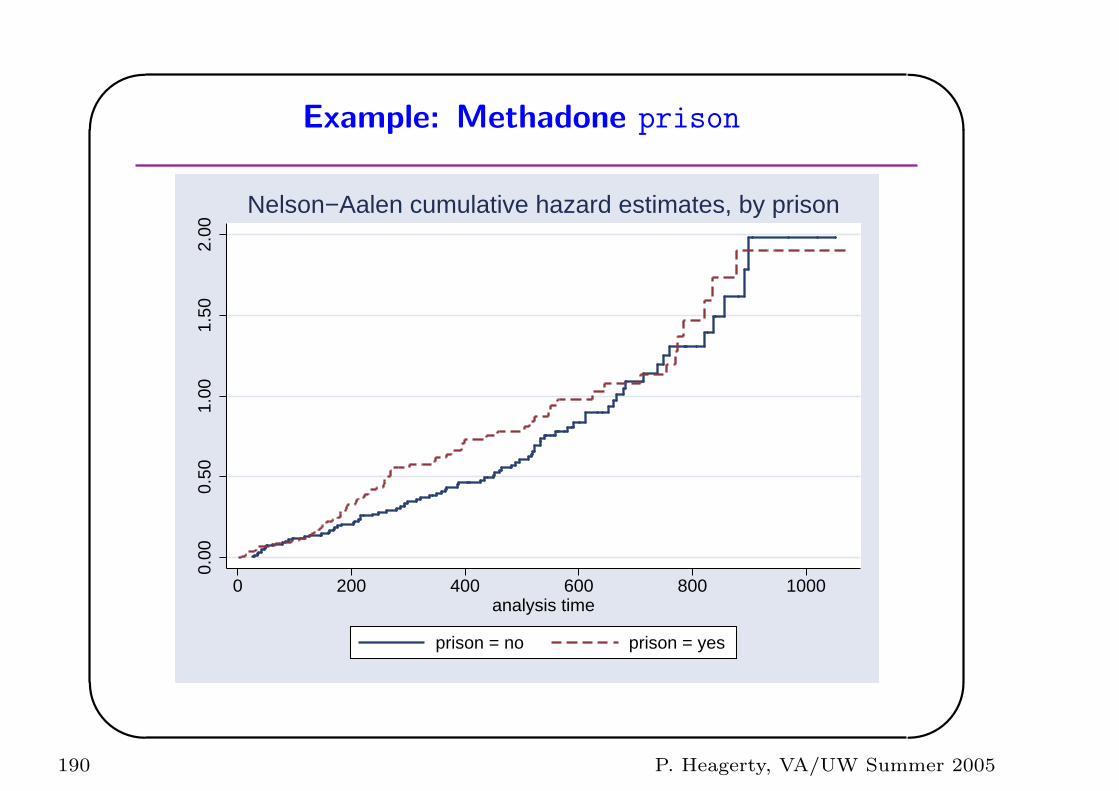
'
&
$
%
Example: Methadone prison
0.00
0.50
1.00
1.50
2.00
0 200 400 600 800 1000analysis time
prison = no prison = yes
Nelson−Aalen cumulative hazard estimates, by prison
190 P. Heagerty, VA/UW Summer 2005
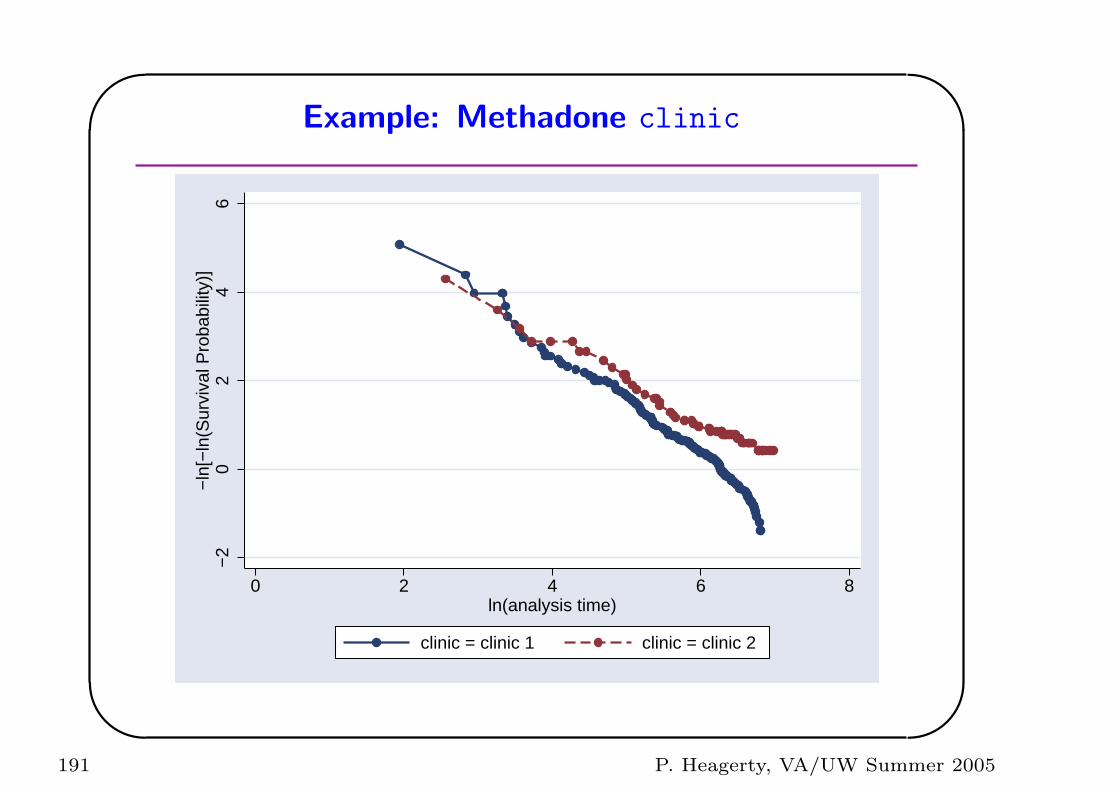
'
&
$
%
Example: Methadone clinic
−2
02
46
−ln
[−ln
(Sur
viva
l Pro
babi
lity)
]
0 2 4 6 8ln(analysis time)
clinic = clinic 1 clinic = clinic 2
191 P. Heagerty, VA/UW Summer 2005
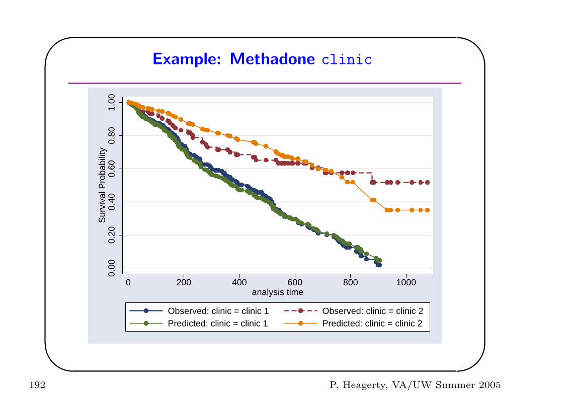
'
&
$
%
Example: Methadone clinic
0.00
0.20
0.40
0.60
0.80
1.00
Sur
viva
l Pro
babi
lity
0 200 400 600 800 1000analysis time
Observed: clinic = clinic 1 Observed: clinic = clinic 2Predicted: clinic = clinic 1 Predicted: clinic = clinic 2
192 P. Heagerty, VA/UW Summer 2005
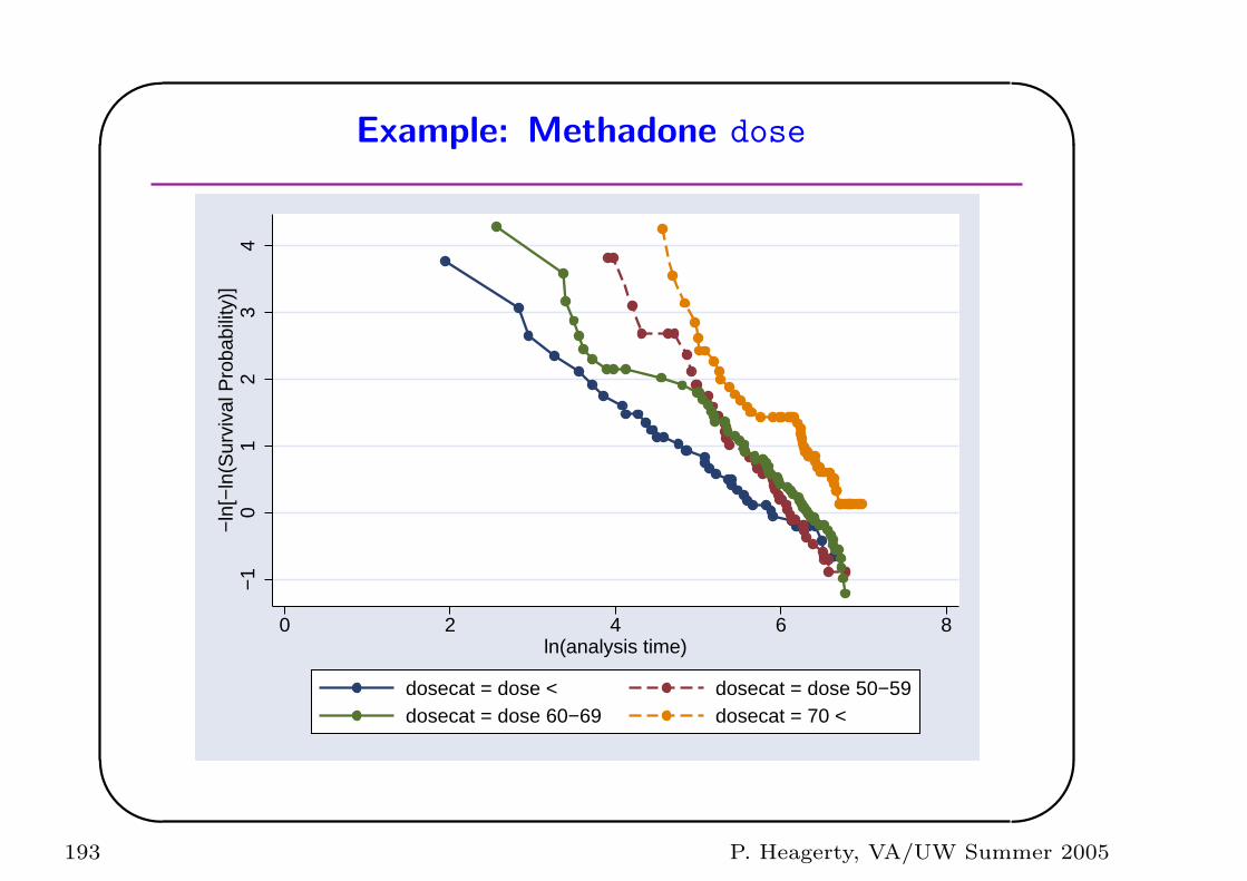
'
&
$
%
Example: Methadone dose
−1
01
23
4−
ln[−
ln(S
urvi
val P
roba
bilit
y)]
0 2 4 6 8ln(analysis time)
dosecat = dose < dosecat = dose 50−59dosecat = dose 60−69 dosecat = 70 <
193 P. Heagerty, VA/UW Summer 2005
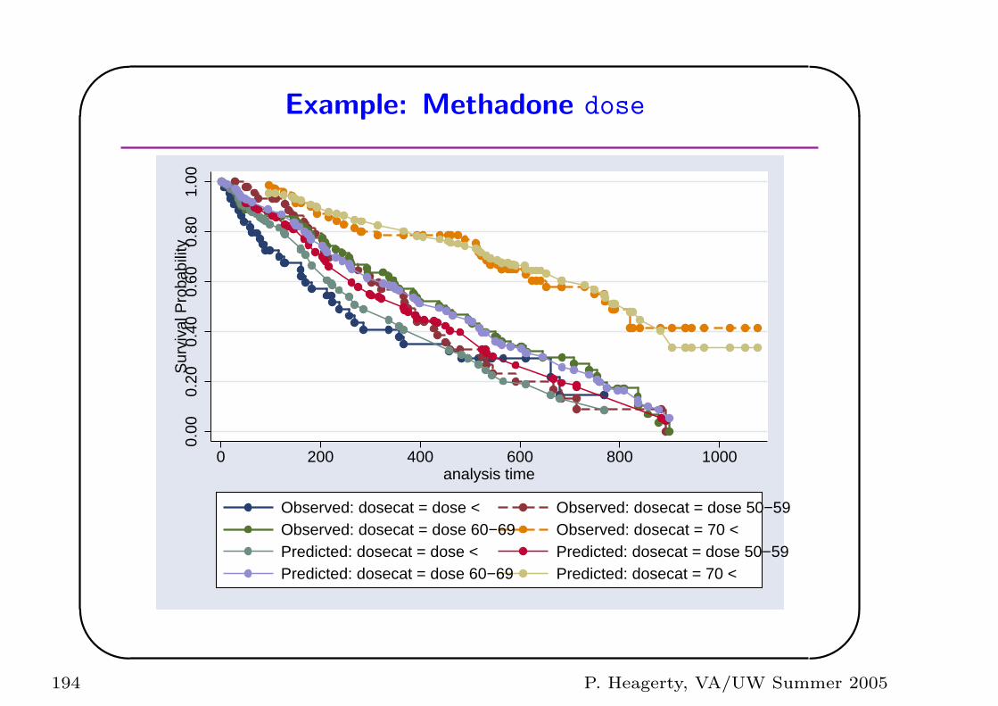
'
&
$
%
Example: Methadone dose
0.00
0.20
0.40
0.60
0.80
1.00
Sur
viva
l Pro
babi
lity
0 200 400 600 800 1000analysis time
Observed: dosecat = dose < Observed: dosecat = dose 50−59Observed: dosecat = dose 60−69 Observed: dosecat = 70 <Predicted: dosecat = dose < Predicted: dosecat = dose 50−59Predicted: dosecat = dose 60−69 Predicted: dosecat = 70 <
194 P. Heagerty, VA/UW Summer 2005
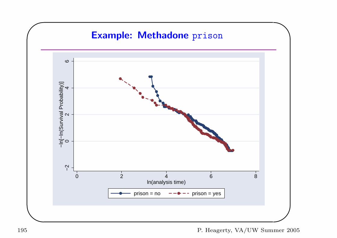
'
&
$
%
Example: Methadone prison
−2
02
46
−ln
[−ln
(Sur
viva
l Pro
babi
lity)
]
0 2 4 6 8ln(analysis time)
prison = no prison = yes
195 P. Heagerty, VA/UW Summer 2005
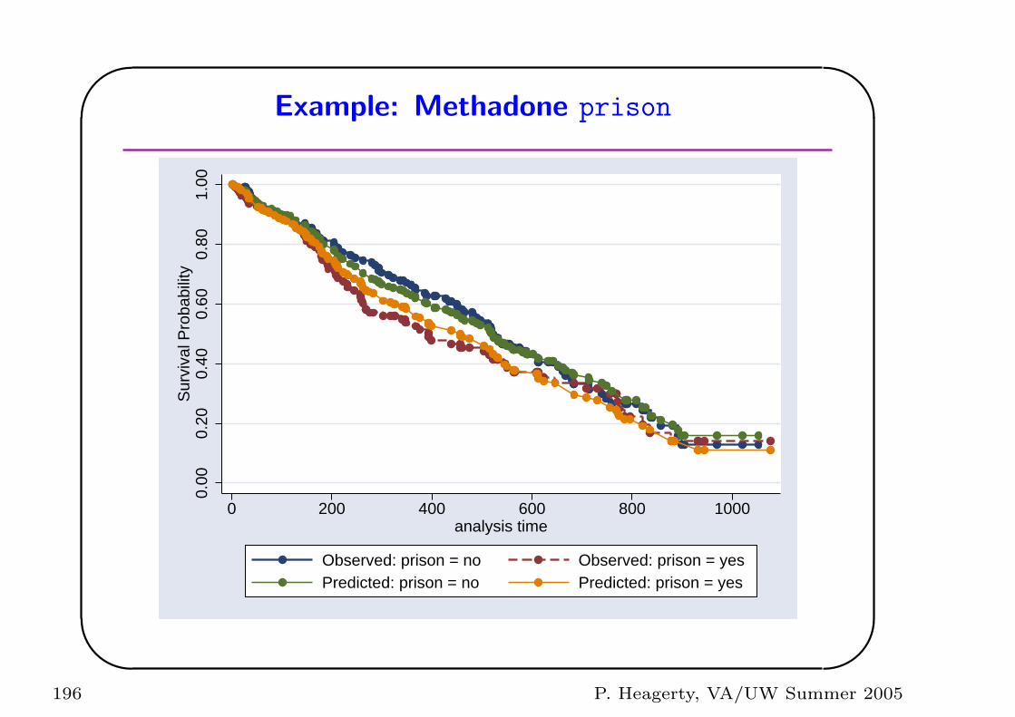
'
&
$
%
Example: Methadone prison
0.00
0.20
0.40
0.60
0.80
1.00
Sur
viva
l Pro
babi
lity
0 200 400 600 800 1000analysis time
Observed: prison = no Observed: prison = yesPredicted: prison = no Predicted: prison = yes
196 P. Heagerty, VA/UW Summer 2005
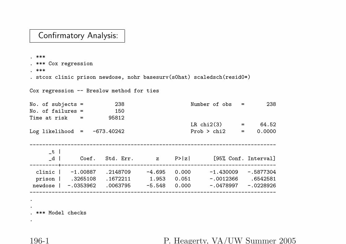
Confirmatory Analysis:
. ***
. *** Cox regression
. ***
. stcox clinic prison newdose, nohr basesurv(s0hat) scaledsch(resid0*)
Cox regression -- Breslow method for ties
No. of subjects = 238 Number of obs = 238No. of failures = 150Time at risk = 95812
LR chi2(3) = 64.52Log likelihood = -673.40242 Prob > chi2 = 0.0000
------------------------------------------------------------------------------_t |_d | Coef. Std. Err. z P>|z| [95% Conf. Interval]
---------+--------------------------------------------------------------------clinic | -1.00887 .2148709 -4.695 0.000 -1.430009 -.5877304prison | .3265108 .1672211 1.953 0.051 -.0012366 .6542581
newdose | -.0353962 .0063795 -5.548 0.000 -.0478997 -.0228926------------------------------------------------------------------------------... *** Model checks.
196-1 P. Heagerty, VA/UW Summer 2005
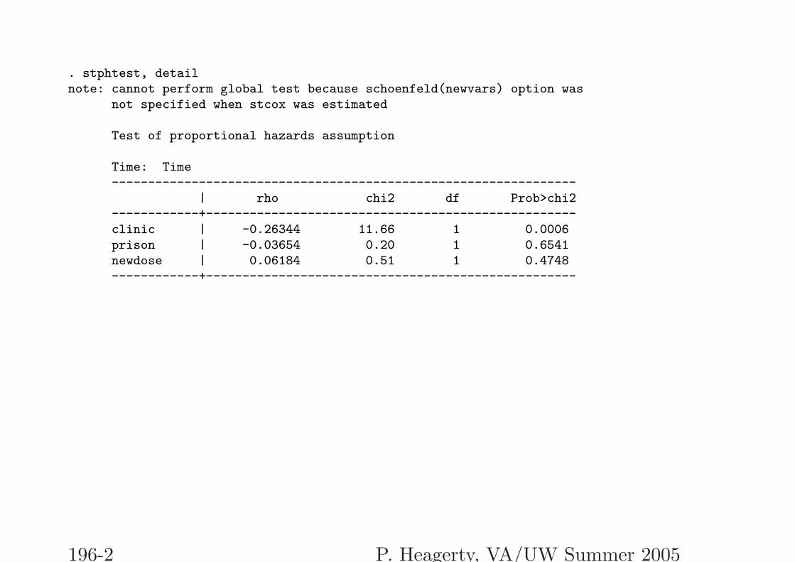
. stphtest, detailnote: cannot perform global test because schoenfeld(newvars) option was
not specified when stcox was estimated
Test of proportional hazards assumption
Time: Time----------------------------------------------------------------
| rho chi2 df Prob>chi2------------+---------------------------------------------------clinic | -0.26344 11.66 1 0.0006prison | -0.03654 0.20 1 0.6541newdose | 0.06184 0.51 1 0.4748------------+---------------------------------------------------
196-2 P. Heagerty, VA/UW Summer 2005
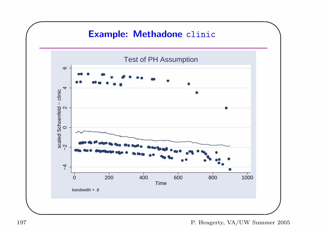
'
&
$
%
Example: Methadone clinic
−4
−2
02
46
scal
ed S
choe
nfel
d −
clin
ic
0 200 400 600 800 1000Time
bandwidth = .8
Test of PH Assumption
197 P. Heagerty, VA/UW Summer 2005
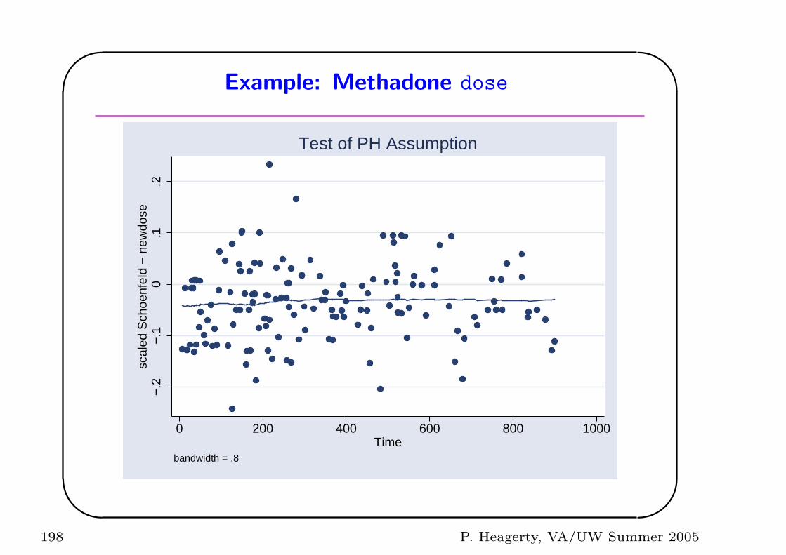
'
&
$
%
Example: Methadone dose
−.2
−.1
0.1
.2sc
aled
Sch
oenf
eld
− n
ewdo
se
0 200 400 600 800 1000Time
bandwidth = .8
Test of PH Assumption
198 P. Heagerty, VA/UW Summer 2005
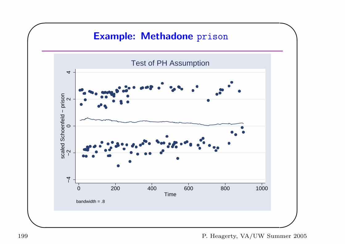
'
&
$
%
Example: Methadone prison
−4
−2
02
4sc
aled
Sch
oenf
eld
− p
rison
0 200 400 600 800 1000Time
bandwidth = .8
Test of PH Assumption
199 P. Heagerty, VA/UW Summer 2005
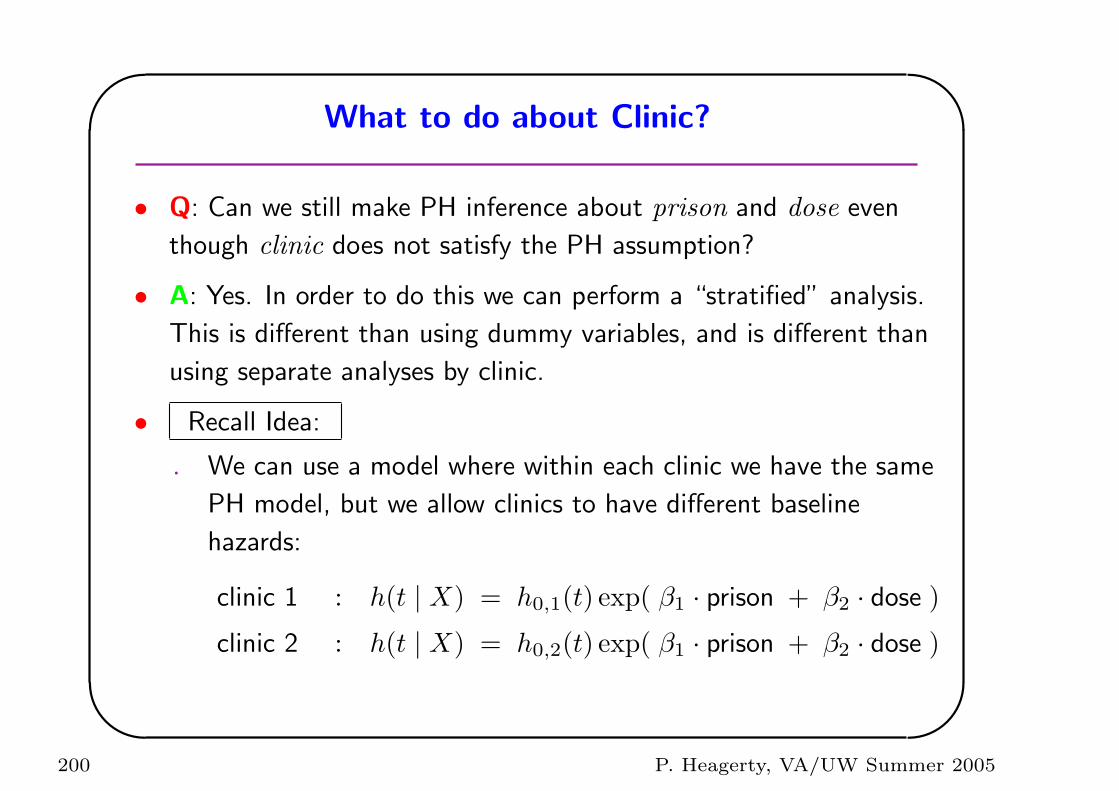
'
&
$
%
What to do about Clinic?
• Q: Can we still make PH inference about prison and dose even
though clinic does not satisfy the PH assumption?
• A: Yes. In order to do this we can perform a “stratified” analysis.
This is different than using dummy variables, and is different than
using separate analyses by clinic.
• Recall Idea:
. We can use a model where within each clinic we have the same
PH model, but we allow clinics to have different baseline
hazards:
clinic 1 : h(t | X) = h0,1(t) exp( β1 · prison + β2 · dose )
clinic 2 : h(t | X) = h0,2(t) exp( β1 · prison + β2 · dose )
200 P. Heagerty, VA/UW Summer 2005
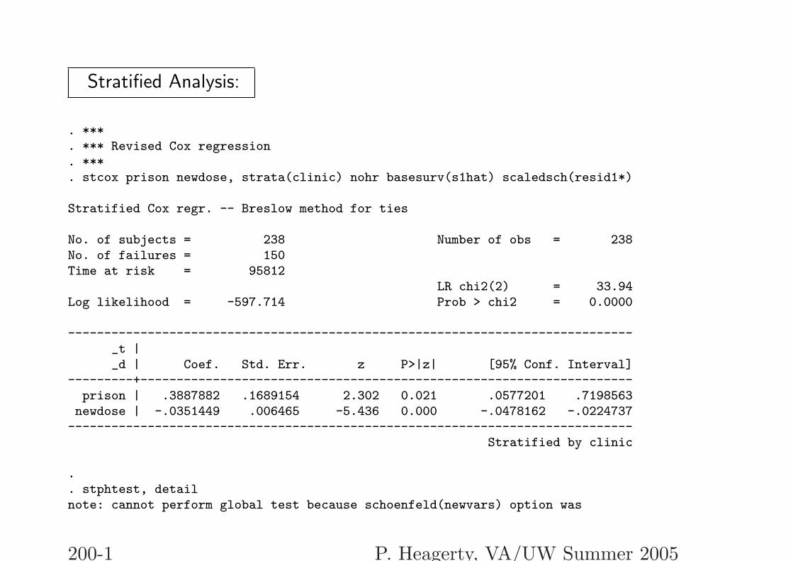
Stratified Analysis:
. ***
. *** Revised Cox regression
. ***
. stcox prison newdose, strata(clinic) nohr basesurv(s1hat) scaledsch(resid1*)
Stratified Cox regr. -- Breslow method for ties
No. of subjects = 238 Number of obs = 238No. of failures = 150Time at risk = 95812
LR chi2(2) = 33.94Log likelihood = -597.714 Prob > chi2 = 0.0000
------------------------------------------------------------------------------_t |_d | Coef. Std. Err. z P>|z| [95% Conf. Interval]
---------+--------------------------------------------------------------------prison | .3887882 .1689154 2.302 0.021 .0577201 .7198563
newdose | -.0351449 .006465 -5.436 0.000 -.0478162 -.0224737------------------------------------------------------------------------------
Stratified by clinic
.
. stphtest, detailnote: cannot perform global test because schoenfeld(newvars) option was
200-1 P. Heagerty, VA/UW Summer 2005
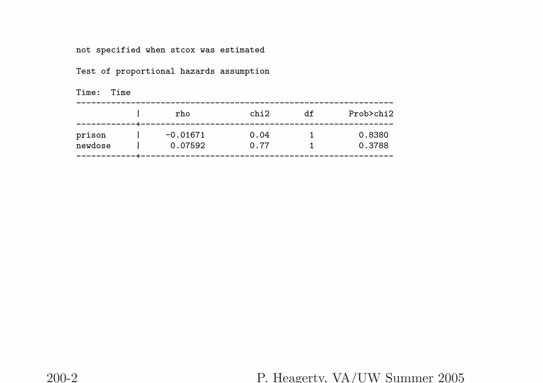
not specified when stcox was estimated
Test of proportional hazards assumption
Time: Time----------------------------------------------------------------
| rho chi2 df Prob>chi2------------+---------------------------------------------------prison | -0.01671 0.04 1 0.8380newdose | 0.07592 0.77 1 0.3788------------+---------------------------------------------------
200-2 P. Heagerty, VA/UW Summer 2005
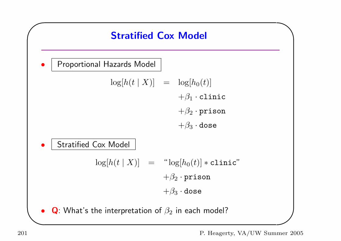
'
&
$
%
Stratified Cox Model
• Proportional Hazards Model
log[h(t | X)] = log[h0(t)]
+β1 · clinic+β2 · prison+β3 · dose
• Stratified Cox Model
log[h(t | X)] = “ log[h0(t)] ∗ clinic”+β2 · prison+β3 · dose
• Q: What’s the interpretation of β2 in each model?
201 P. Heagerty, VA/UW Summer 2005
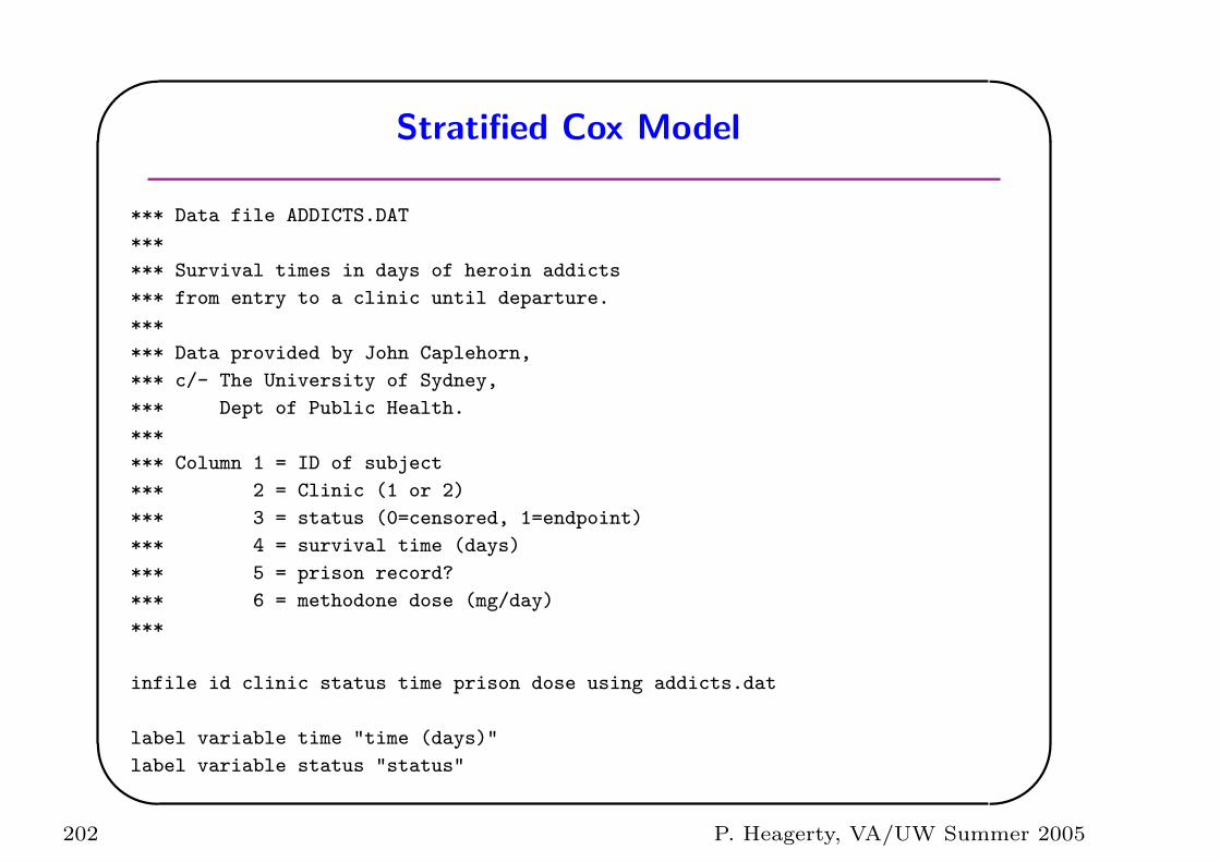
'
&
$
%
Stratified Cox Model
*** Data file ADDICTS.DAT
***
*** Survival times in days of heroin addicts
*** from entry to a clinic until departure.
***
*** Data provided by John Caplehorn,
*** c/- The University of Sydney,
*** Dept of Public Health.
***
*** Column 1 = ID of subject
*** 2 = Clinic (1 or 2)
*** 3 = status (0=censored, 1=endpoint)
*** 4 = survival time (days)
*** 5 = prison record?
*** 6 = methodone dose (mg/day)
***
infile id clinic status time prison dose using addicts.dat
label variable time "time (days)"
label variable status "status"
202 P. Heagerty, VA/UW Summer 2005
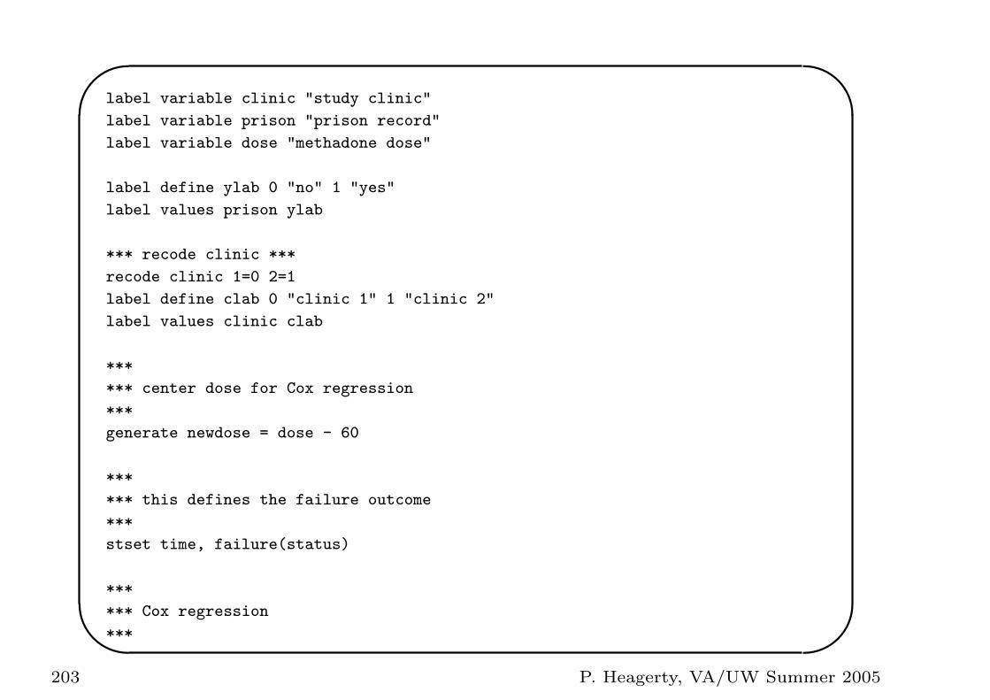
'
&
$
%
label variable clinic "study clinic"
label variable prison "prison record"
label variable dose "methadone dose"
label define ylab 0 "no" 1 "yes"
label values prison ylab
*** recode clinic ***
recode clinic 1=0 2=1
label define clab 0 "clinic 1" 1 "clinic 2"
label values clinic clab
***
*** center dose for Cox regression
***
generate newdose = dose - 60
***
*** this defines the failure outcome
***
stset time, failure(status)
***
*** Cox regression
***
203 P. Heagerty, VA/UW Summer 2005
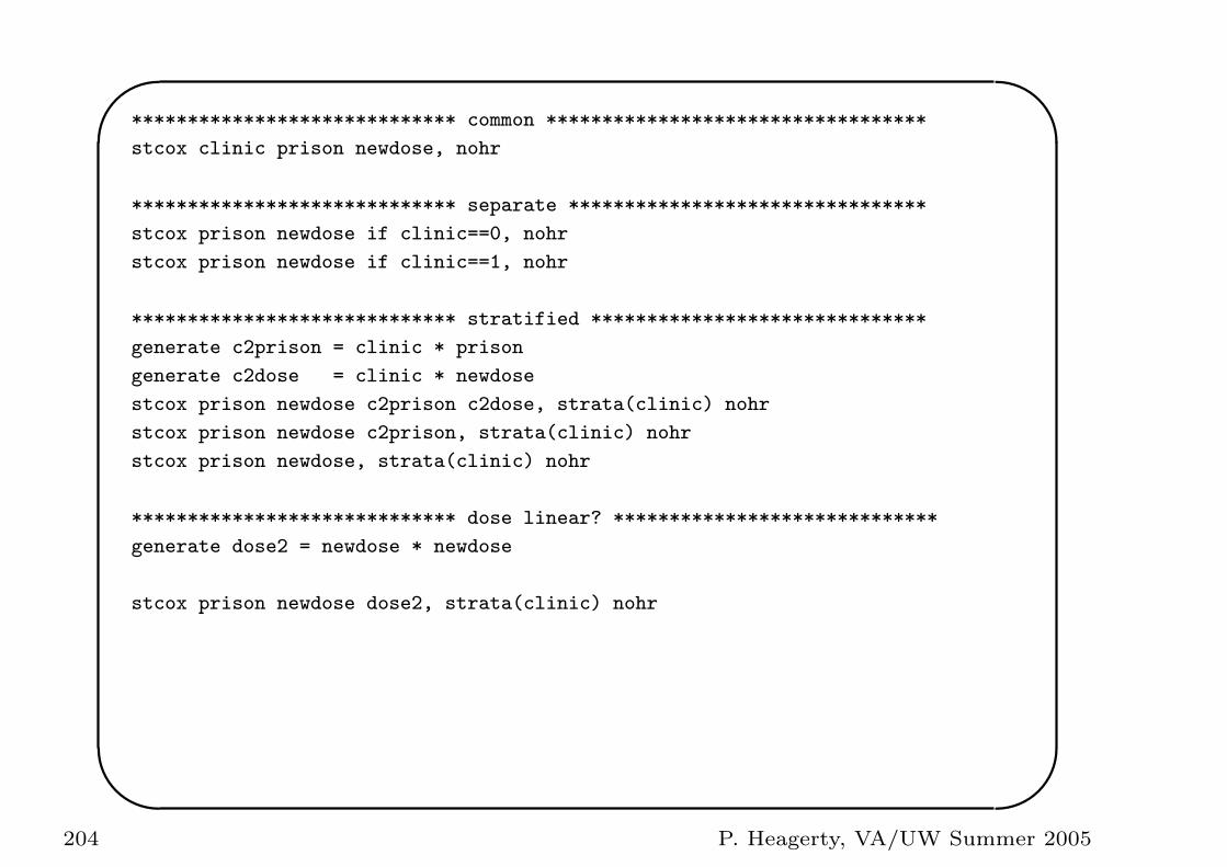
'
&
$
%
***************************** common **********************************
stcox clinic prison newdose, nohr
***************************** separate ********************************
stcox prison newdose if clinic==0, nohr
stcox prison newdose if clinic==1, nohr
***************************** stratified ******************************
generate c2prison = clinic * prison
generate c2dose = clinic * newdose
stcox prison newdose c2prison c2dose, strata(clinic) nohr
stcox prison newdose c2prison, strata(clinic) nohr
stcox prison newdose, strata(clinic) nohr
***************************** dose linear? *****************************
generate dose2 = newdose * newdose
stcox prison newdose dose2, strata(clinic) nohr
204 P. Heagerty, VA/UW Summer 2005
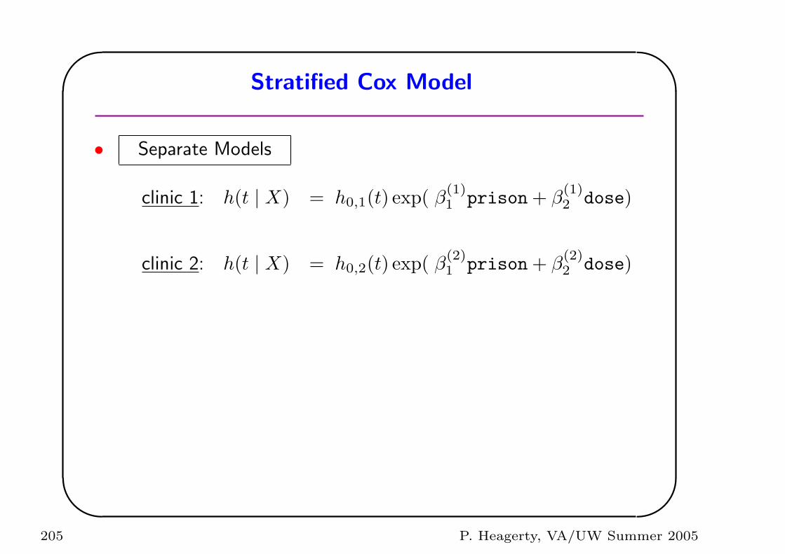
'
&
$
%
Stratified Cox Model
• Separate Models
clinic 1: h(t | X) = h0,1(t) exp( β(1)1 prison + β
(1)2 dose)
clinic 2: h(t | X) = h0,2(t) exp( β(2)1 prison + β
(2)2 dose)
205 P. Heagerty, VA/UW Summer 2005
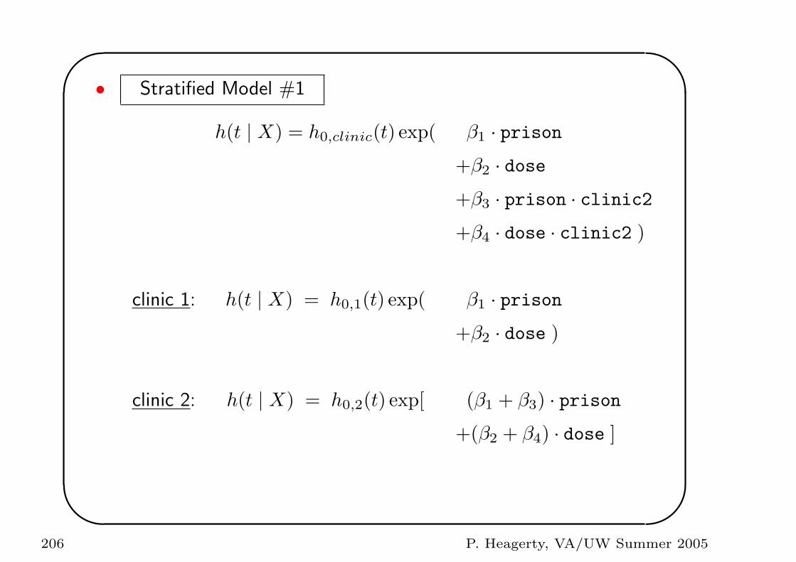
'
&
$
%
• Stratified Model #1
h(t | X) = h0,clinic(t) exp( β1 · prison+β2 · dose+β3 · prison · clinic2+β4 · dose · clinic2 )
clinic 1: h(t | X) = h0,1(t) exp( β1 · prison+β2 · dose )
clinic 2: h(t | X) = h0,2(t) exp[ (β1 + β3) · prison+(β2 + β4) · dose ]
206 P. Heagerty, VA/UW Summer 2005
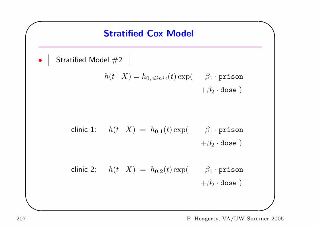
'
&
$
%
Stratified Cox Model
• Stratified Model #2
h(t | X) = h0,clinic(t) exp( β1 · prison+β2 · dose )
clinic 1: h(t | X) = h0,1(t) exp( β1 · prison+β2 · dose )
clinic 2: h(t | X) = h0,2(t) exp( β1 · prison+β2 · dose )
207 P. Heagerty, VA/UW Summer 2005
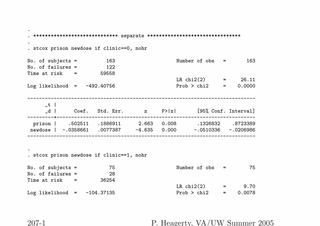
.
. ***************************** separate ********************************
.
. stcox prison newdose if clinic==0, nohr
No. of subjects = 163 Number of obs = 163No. of failures = 122Time at risk = 59558
LR chi2(2) = 26.11Log likelihood = -492.40756 Prob > chi2 = 0.0000
------------------------------------------------------------------------------_t |_d | Coef. Std. Err. z P>|z| [95% Conf. Interval]
---------+--------------------------------------------------------------------prison | .502511 .1886911 2.663 0.008 .1326832 .8723389
newdose | -.0358661 .0077387 -4.635 0.000 -.0510336 -.0206986------------------------------------------------------------------------------
.
. stcox prison newdose if clinic==1, nohr
No. of subjects = 75 Number of obs = 75No. of failures = 28Time at risk = 36254
LR chi2(2) = 9.70Log likelihood = -104.37135 Prob > chi2 = 0.0078
207-1 P. Heagerty, VA/UW Summer 2005
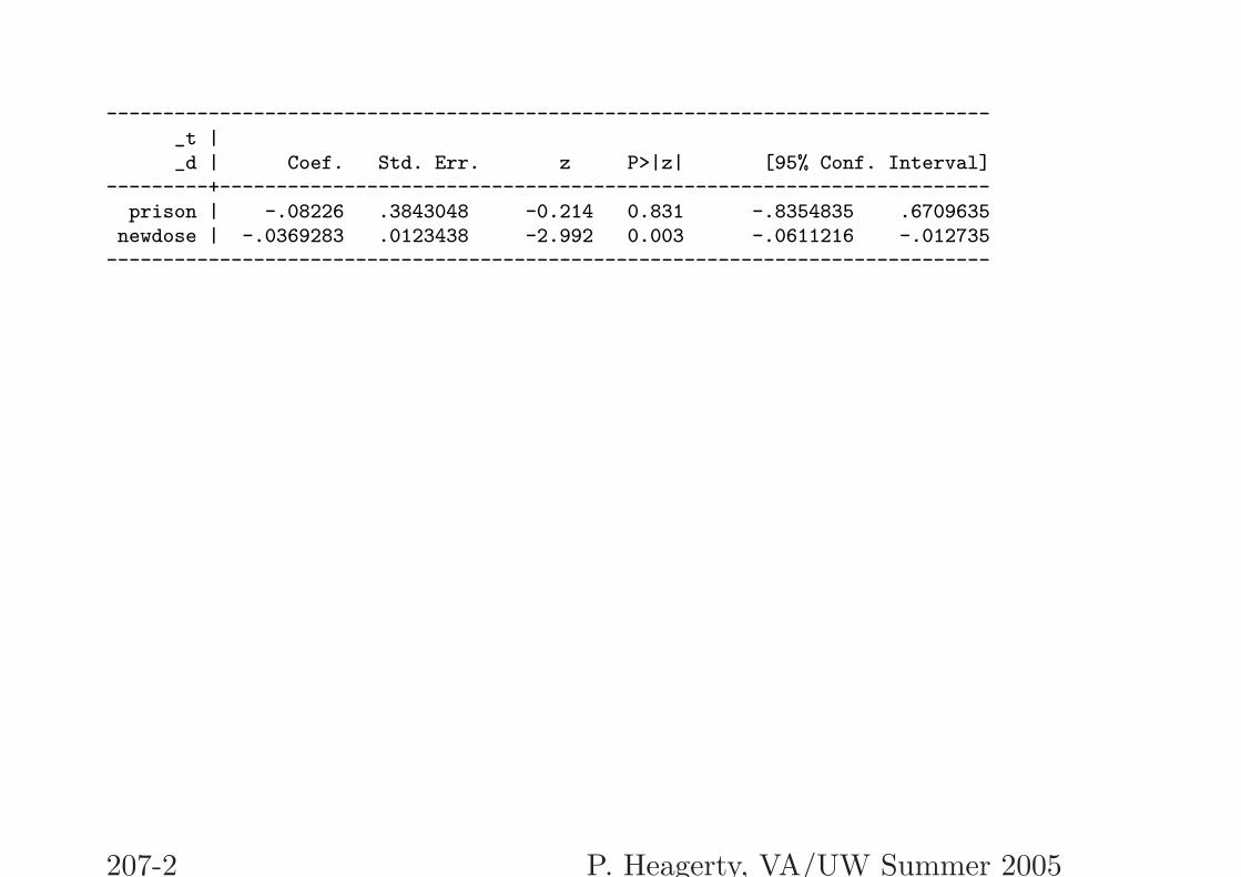
------------------------------------------------------------------------------_t |_d | Coef. Std. Err. z P>|z| [95% Conf. Interval]
---------+--------------------------------------------------------------------prison | -.08226 .3843048 -0.214 0.831 -.8354835 .6709635
newdose | -.0369283 .0123438 -2.992 0.003 -.0611216 -.012735------------------------------------------------------------------------------
207-2 P. Heagerty, VA/UW Summer 2005
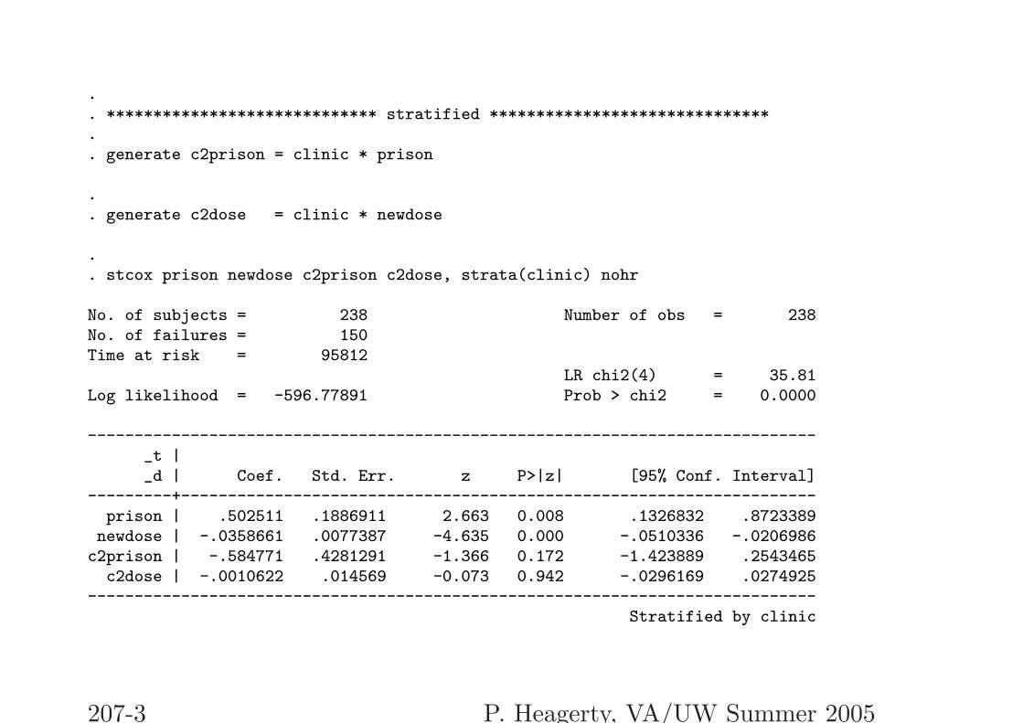
.
. ***************************** stratified ******************************
.
. generate c2prison = clinic * prison
.
. generate c2dose = clinic * newdose
.
. stcox prison newdose c2prison c2dose, strata(clinic) nohr
No. of subjects = 238 Number of obs = 238No. of failures = 150Time at risk = 95812
LR chi2(4) = 35.81Log likelihood = -596.77891 Prob > chi2 = 0.0000
------------------------------------------------------------------------------_t |_d | Coef. Std. Err. z P>|z| [95% Conf. Interval]
---------+--------------------------------------------------------------------prison | .502511 .1886911 2.663 0.008 .1326832 .8723389
newdose | -.0358661 .0077387 -4.635 0.000 -.0510336 -.0206986c2prison | -.584771 .4281291 -1.366 0.172 -1.423889 .2543465
c2dose | -.0010622 .014569 -0.073 0.942 -.0296169 .0274925------------------------------------------------------------------------------
Stratified by clinic
207-3 P. Heagerty, VA/UW Summer 2005
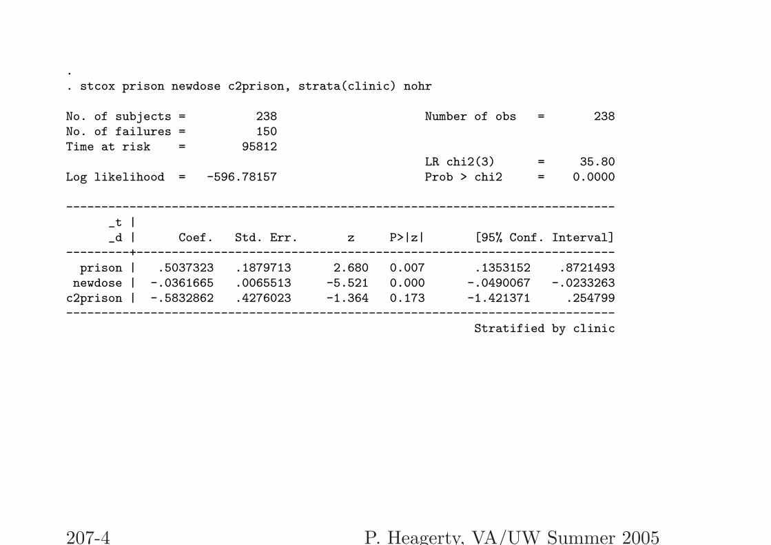
.
. stcox prison newdose c2prison, strata(clinic) nohr
No. of subjects = 238 Number of obs = 238No. of failures = 150Time at risk = 95812
LR chi2(3) = 35.80Log likelihood = -596.78157 Prob > chi2 = 0.0000
------------------------------------------------------------------------------_t |_d | Coef. Std. Err. z P>|z| [95% Conf. Interval]
---------+--------------------------------------------------------------------prison | .5037323 .1879713 2.680 0.007 .1353152 .8721493
newdose | -.0361665 .0065513 -5.521 0.000 -.0490067 -.0233263c2prison | -.5832862 .4276023 -1.364 0.173 -1.421371 .254799------------------------------------------------------------------------------
Stratified by clinic
207-4 P. Heagerty, VA/UW Summer 2005
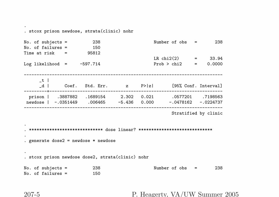
.
. stcox prison newdose, strata(clinic) nohr
No. of subjects = 238 Number of obs = 238No. of failures = 150Time at risk = 95812
LR chi2(2) = 33.94Log likelihood = -597.714 Prob > chi2 = 0.0000
------------------------------------------------------------------------------_t |_d | Coef. Std. Err. z P>|z| [95% Conf. Interval]
---------+--------------------------------------------------------------------prison | .3887882 .1689154 2.302 0.021 .0577201 .7198563
newdose | -.0351449 .006465 -5.436 0.000 -.0478162 -.0224737------------------------------------------------------------------------------
Stratified by clinic
.
. ***************************** dose linear? *****************************
.
. generate dose2 = newdose * newdose
.
. stcox prison newdose dose2, strata(clinic) nohr
No. of subjects = 238 Number of obs = 238No. of failures = 150
207-5 P. Heagerty, VA/UW Summer 2005
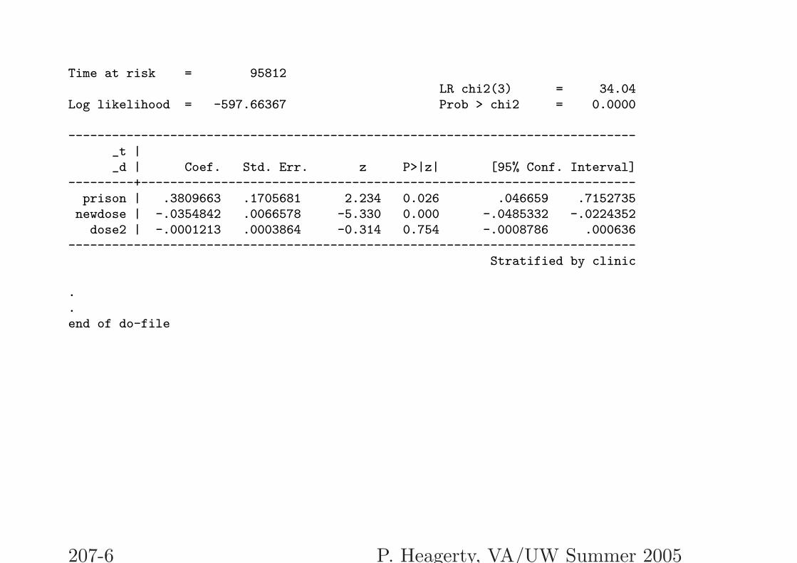
Time at risk = 95812LR chi2(3) = 34.04
Log likelihood = -597.66367 Prob > chi2 = 0.0000
------------------------------------------------------------------------------_t |_d | Coef. Std. Err. z P>|z| [95% Conf. Interval]
---------+--------------------------------------------------------------------prison | .3809663 .1705681 2.234 0.026 .046659 .7152735
newdose | -.0354842 .0066578 -5.330 0.000 -.0485332 -.0224352dose2 | -.0001213 .0003864 -0.314 0.754 -.0008786 .000636
------------------------------------------------------------------------------Stratified by clinic
.
.end of do-file
207-6 P. Heagerty, VA/UW Summer 2005
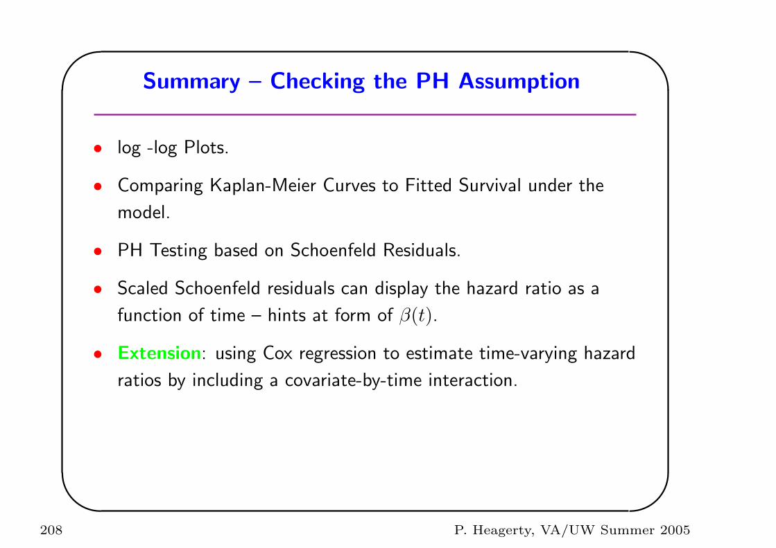
'
&
$
%
Summary – Checking the PH Assumption
• log -log Plots.
• Comparing Kaplan-Meier Curves to Fitted Survival under the
model.
• PH Testing based on Schoenfeld Residuals.
• Scaled Schoenfeld residuals can display the hazard ratio as a
function of time – hints at form of β(t).
• Extension: using Cox regression to estimate time-varying hazard
ratios by including a covariate-by-time interaction.
208 P. Heagerty, VA/UW Summer 2005
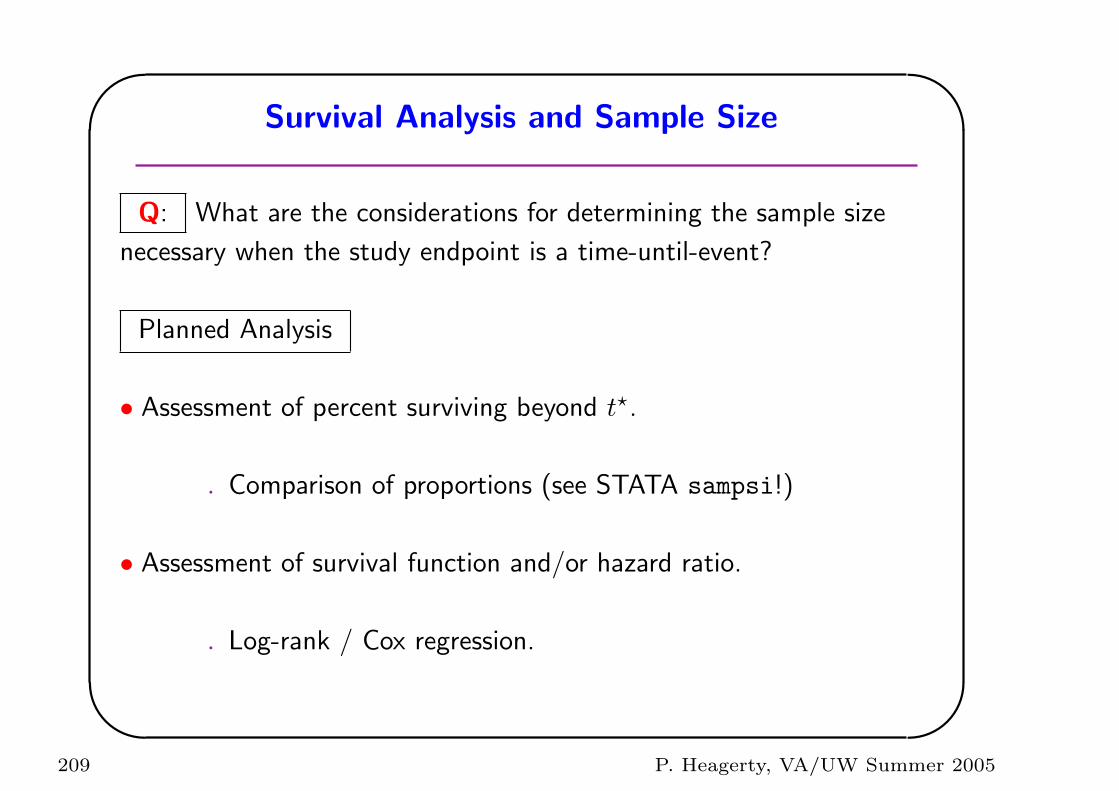
'
&
$
%
Survival Analysis and Sample Size
Q: What are the considerations for determining the sample size
necessary when the study endpoint is a time-until-event?
Planned Analysis
• Assessment of percent surviving beyond t?.
. Comparison of proportions (see STATA sampsi!)
• Assessment of survival function and/or hazard ratio.
. Log-rank / Cox regression.
209 P. Heagerty, VA/UW Summer 2005
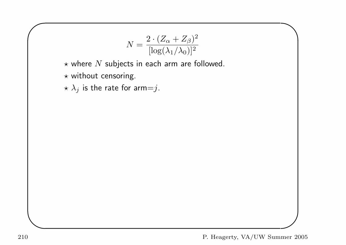
'
&
$
%
N =2 · (Zα + Zβ)2
[log(λ1/λ0)]2
? where N subjects in each arm are followed.
? without censoring.
? λj is the rate for arm=j.
210 P. Heagerty, VA/UW Summer 2005
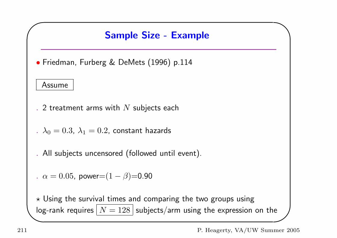
'
&
$
%
Sample Size - Example
• Friedman, Furberg & DeMets (1996) p.114
Assume
. 2 treatment arms with N subjects each
. λ0 = 0.3, λ1 = 0.2, constant hazards
. All subjects uncensored (followed until event).
. α = 0.05, power=(1− β)=0.90
? Using the survival times and comparing the two groups using
log-rank requires N = 128 subjects/arm using the expression on the
211 P. Heagerty, VA/UW Summer 2005
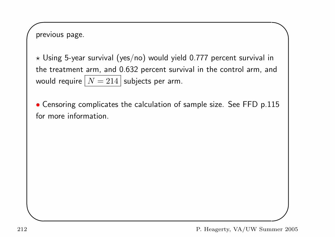
'
&
$
%
previous page.
? Using 5-year survival (yes/no) would yield 0.777 percent survival in
the treatment arm, and 0.632 percent survival in the control arm, and
would require N = 214 subjects per arm.
• Censoring complicates the calculation of sample size. See FFD p.115
for more information.
212 P. Heagerty, VA/UW Summer 2005
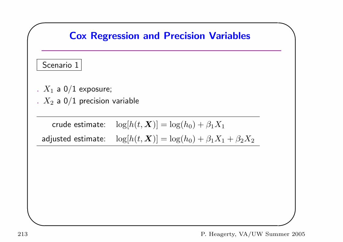
'
&
$
%
Cox Regression and Precision Variables
Scenario 1
. X1 a 0/1 exposure;
. X2 a 0/1 precision variable
crude estimate: log[h(t,X)] = log(h0) + β1X1
adjusted estimate: log[h(t,X)] = log(h0) + β1X1 + β2X2
213 P. Heagerty, VA/UW Summer 2005
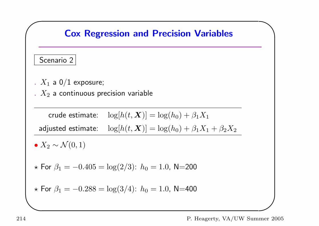
'
&
$
%
Cox Regression and Precision Variables
Scenario 2
. X1 a 0/1 exposure;
. X2 a continuous precision variable
crude estimate: log[h(t,X)] = log(h0) + β1X1
adjusted estimate: log[h(t,X)] = log(h0) + β1X1 + β2X2
• X2 ∼ N (0, 1)
? For β1 = −0.405 = log(2/3): h0 = 1.0, N=200
? For β1 = −0.288 = log(3/4): h0 = 1.0, N=400
214 P. Heagerty, VA/UW Summer 2005
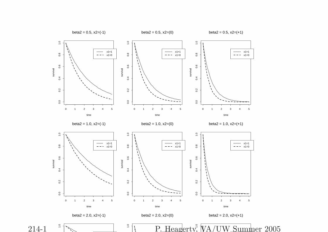
time
surv
ival
0 1 2 3 4 5
0.0
0.2
0.4
0.6
0.8
1.0
x1=1x1=0
beta2 = 0.5, x2=(-1)
time
surv
ival
0 1 2 3 4 5
0.0
0.2
0.4
0.6
0.8
1.0
x1=1x1=0
beta2 = 0.5, x2=(0)
time
surv
ival
0 1 2 3 4 5
0.0
0.2
0.4
0.6
0.8
1.0
x1=1x1=0
beta2 = 0.5, x2=(+1)
time
surv
ival
0 1 2 3 4 5
0.0
0.2
0.4
0.6
0.8
1.0
x1=1x1=0
beta2 = 1.0, x2=(-1)
time
surv
ival
0 1 2 3 4 5
0.0
0.2
0.4
0.6
0.8
1.0
x1=1x1=0
beta2 = 1.0, x2=(0)
time
surv
ival
0 1 2 3 4 5
0.0
0.2
0.4
0.6
0.8
1.0
x1=1x1=0
beta2 = 1.0, x2=(+1)
time
surv
ival
0 1 2 3 4 5
0.0
0.2
0.4
0.6
0.8
1.0
x1=1x1=0
beta2 = 2.0, x2=(-1)
time
surv
ival
0 1 2 3 4 5
0.0
0.2
0.4
0.6
0.8
1.0
x1=1x1=0
beta2 = 2.0, x2=(0)
time
surv
ival
0 1 2 3 4 5
0.0
0.2
0.4
0.6
0.8
1.0
x1=1x1=0
beta2 = 2.0, x2=(+1)
214-1 P. Heagerty, VA/UW Summer 2005
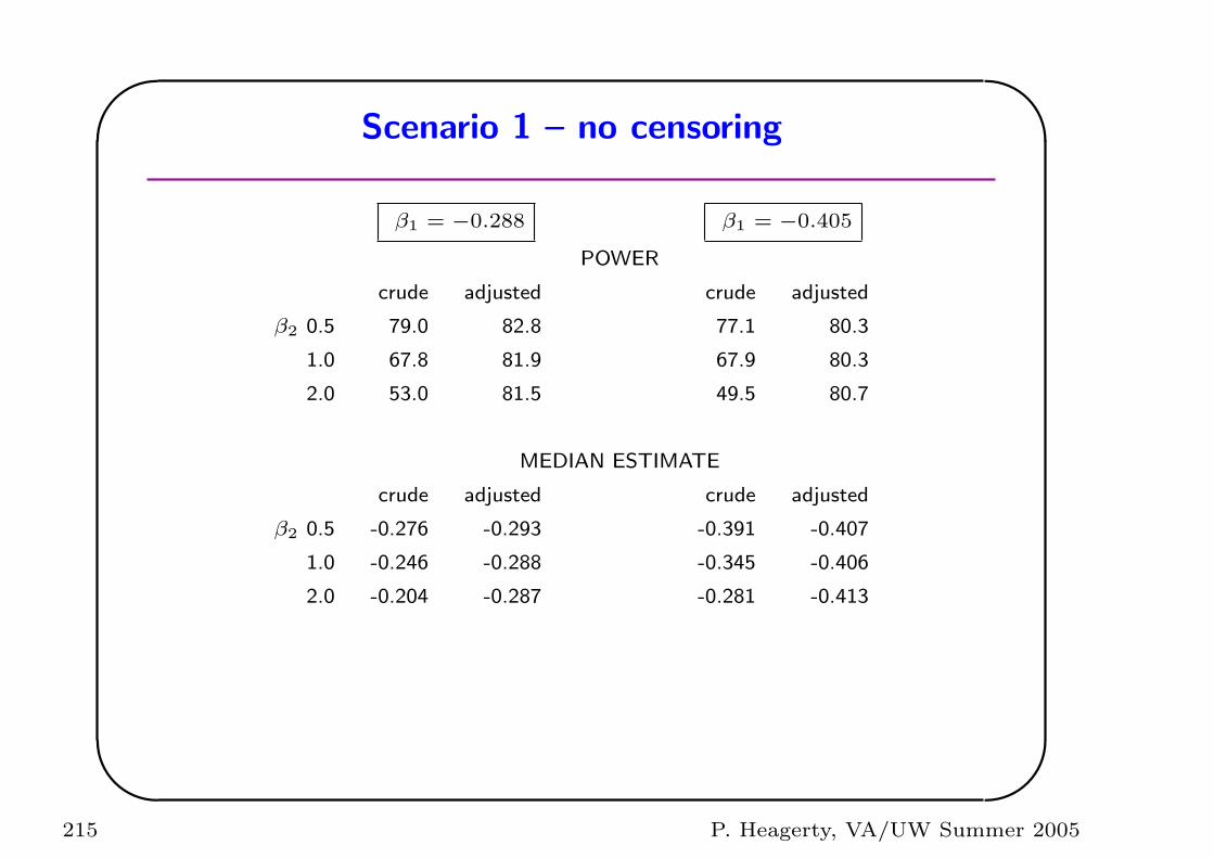
'
&
$
%
Scenario 1 – no censoring
β1 = −0.288 β1 = −0.405
POWER
crude adjusted crude adjusted
β2 0.5 79.0 82.8 77.1 80.3
1.0 67.8 81.9 67.9 80.3
2.0 53.0 81.5 49.5 80.7
MEDIAN ESTIMATE
crude adjusted crude adjusted
β2 0.5 -0.276 -0.293 -0.391 -0.407
1.0 -0.246 -0.288 -0.345 -0.406
2.0 -0.204 -0.287 -0.281 -0.413
215 P. Heagerty, VA/UW Summer 2005
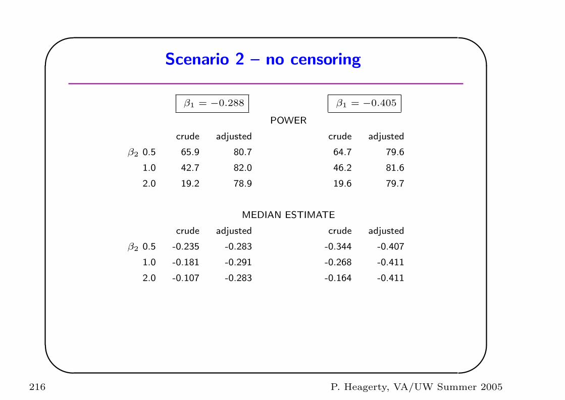
'
&
$
%
Scenario 2 – no censoring
β1 = −0.288 β1 = −0.405
POWER
crude adjusted crude adjusted
β2 0.5 65.9 80.7 64.7 79.6
1.0 42.7 82.0 46.2 81.6
2.0 19.2 78.9 19.6 79.7
MEDIAN ESTIMATE
crude adjusted crude adjusted
β2 0.5 -0.235 -0.283 -0.344 -0.407
1.0 -0.181 -0.291 -0.268 -0.411
2.0 -0.107 -0.283 -0.164 -0.411
216 P. Heagerty, VA/UW Summer 2005
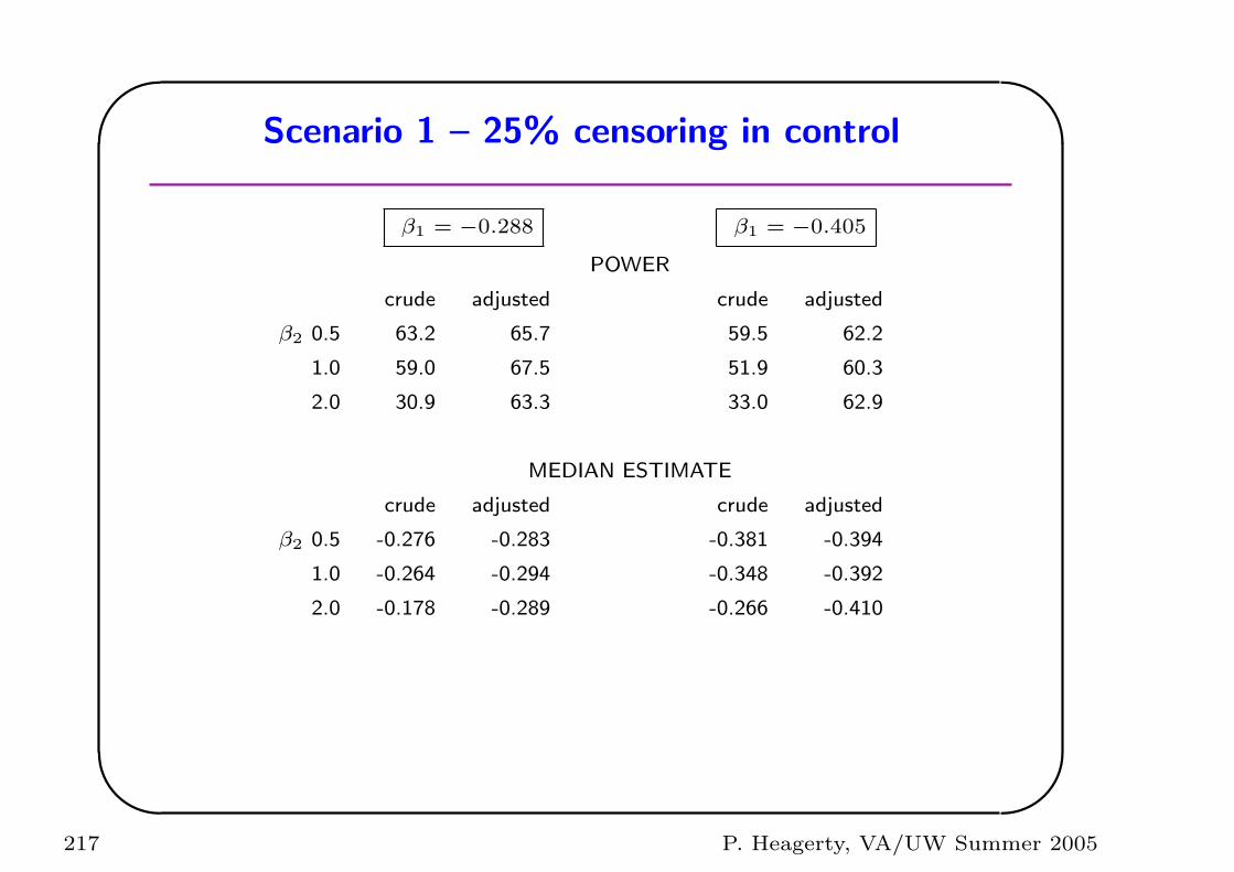
'
&
$
%
Scenario 1 – 25% censoring in control
β1 = −0.288 β1 = −0.405
POWER
crude adjusted crude adjusted
β2 0.5 63.2 65.7 59.5 62.2
1.0 59.0 67.5 51.9 60.3
2.0 30.9 63.3 33.0 62.9
MEDIAN ESTIMATE
crude adjusted crude adjusted
β2 0.5 -0.276 -0.283 -0.381 -0.394
1.0 -0.264 -0.294 -0.348 -0.392
2.0 -0.178 -0.289 -0.266 -0.410
217 P. Heagerty, VA/UW Summer 2005

'
&
$
%
Scenario 2 – 25% censoring in control
β1 = −0.288 β1 = −0.405
POWER
crude adjusted crude adjusted
β2 0.5 56.1 65.4 56.6 64.6
1.0 36.4 63.2 36.8 62.7
2.0 20.8 60.4 17.9 58.5
MEDIAN ESTIMATE
crude adjusted crude adjusted
β2 0.5 -0.256 -0.288 -0.367 -0.401
1.0 -0.202 -0.283 -0.293 -0.408
2.0 -0.136 -0.285 -0.193 -0.409
218 P. Heagerty, VA/UW Summer 2005
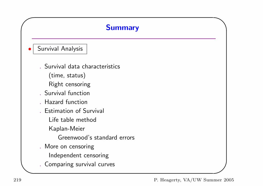
'
&
$
%
Summary
• Survival Analysis
. Survival data characteristics
(time, status)
Right censoring
. Survival function
. Hazard function
. Estimation of Survival
Life table method
Kaplan-Meier
Greenwood’s standard errors
. More on censoring
Independent censoring
. Comparing survival curves
219 P. Heagerty, VA/UW Summer 2005
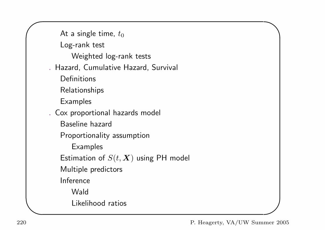
'
&
$
%
At a single time, t0
Log-rank test
Weighted log-rank tests
. Hazard, Cumulative Hazard, Survival
Definitions
Relationships
Examples
. Cox proportional hazards model
Baseline hazard
Proportionality assumption
Examples
Estimation of S(t,X) using PH model
Multiple predictors
Inference
Wald
Likelihood ratios
220 P. Heagerty, VA/UW Summer 2005
'
&
$
%
Estimating hazard ratios
Predictive model building
Checking the PH assumption
log-minus-log plots
Goodness-of-fit tests
Residual plots
Stratified Cox regression
221 P. Heagerty, VA/UW Summer 2005
Related Documents


![[ST] Survival Analysis - Survey Design · 2016. 2. 16. · survival analysis— Introduction to survival analysis 3 Obtaining summary statistics, confidence intervals, tables, etc.](https://static.cupdf.com/doc/110x72/60372d1b619a2a38d04b0197/st-survival-analysis-survey-design-2016-2-16-survival-analysisa-introduction.jpg)