Survival Analysis: Logrank Test Lu Tian and Richard Olshen Stanford University 1

Welcome message from author
This document is posted to help you gain knowledge. Please leave a comment to let me know what you think about it! Share it to your friends and learn new things together.
Transcript

Survival Analysis: Logrank Test
Lu Tian and Richard Olshen
Stanford University
1

Two-sample Comparison
• Objective: to compare survival functions from two groups.
• Requirement: nonparametric, deal with right censoring.
2
Two-sample comparisons
• KM estimators: S1(·) and S0(·)
• Possible test statistics:
sup[0,τ ] |S1(t)− S0(t)|∫ τ
0|S1(t)− S0(t)|dt∫ τ
0{S1(t)− S0(t)}dt
• The null distributions are complex.
3
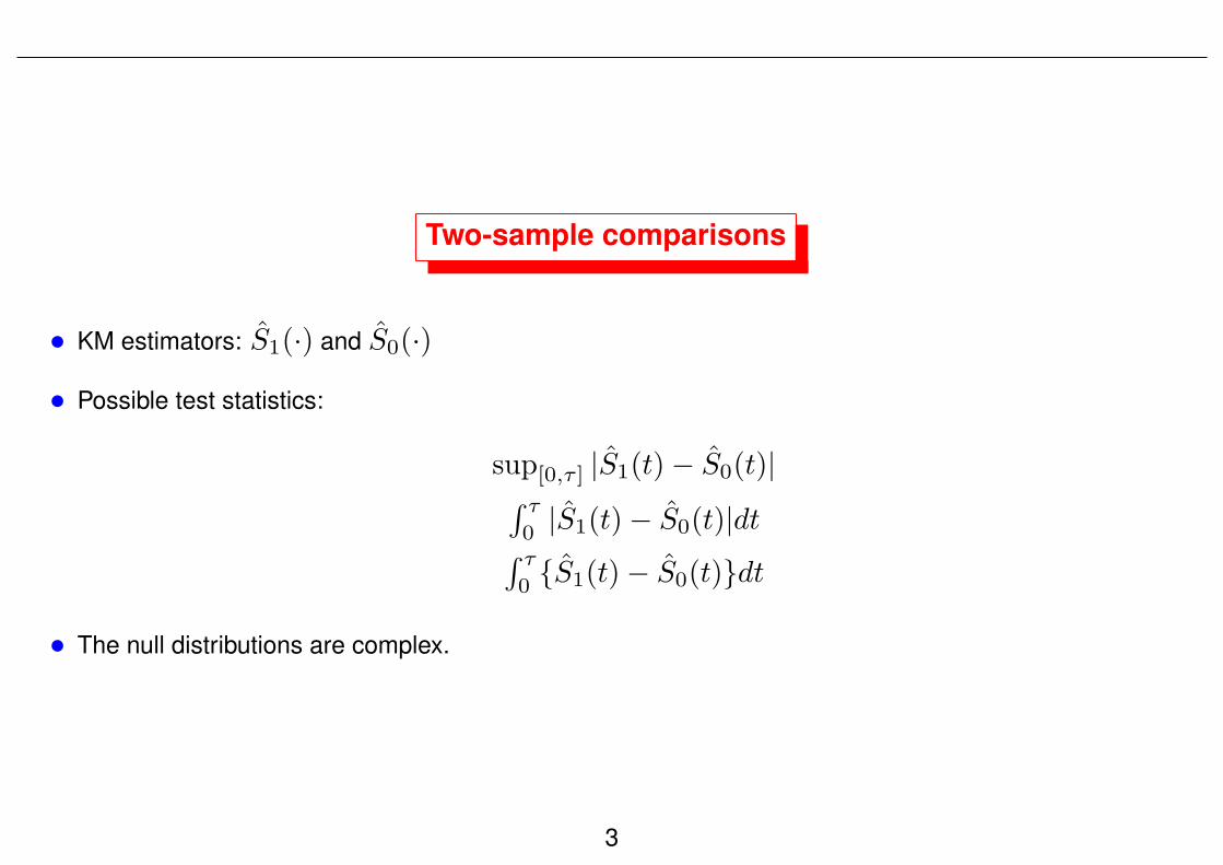
Logrank Test
• The most popular method is the logrank test
1. Adapted from stratified test for 2 by 2 contingency table (Mantel, 1996)
2. Has a nice relationship with the proportional hazards model
3. Targets on the hazard function (not survival function).
4
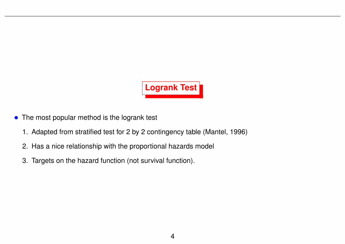
Logrank test
• τ1 < τ2 < · · · < τK are distinct failure times
• Yi(τj) = # persons in group i at risk at τj
• Y (τj) = Y0(τj) + Y1(τj), the total # of subjects at risk at τj
• dij = # of failures in group i at τj
• dj = d0j + d1j total # of failures at τj
5
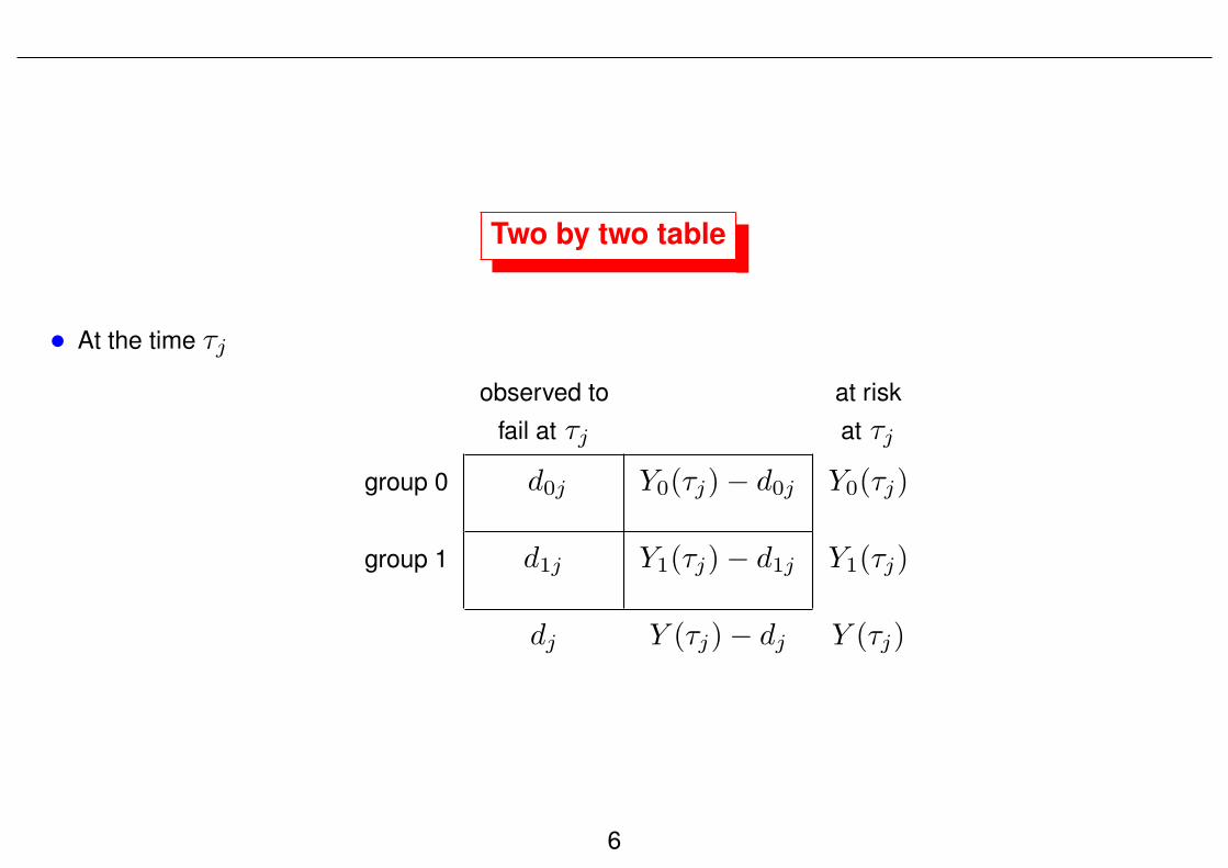
Two by two table
• At the time τj
observed to at risk
fail at τj at τj
group 0 d0j Y0(τj)− d0j Y0(τj)
group 1 d1j Y1(τj)− d1j Y1(τj)
dj Y (τj)− dj Y (τj)
6
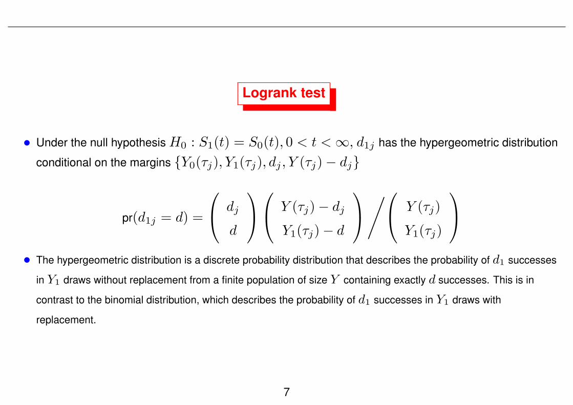
Logrank test
• Under the null hypothesis H0 : S1(t) = S0(t), 0 < t < ∞, d1j has the hypergeometric distribution
conditional on the margins {Y0(τj), Y1(τj), dj , Y (τj)− dj}
pr(d1j = d) =
dj
d
Y (τj)− dj
Y1(τj)− d
/ Y (τj)
Y1(τj)
• The hypergeometric distribution is a discrete probability distribution that describes the probability of d1 successes
in Y1 draws without replacement from a finite population of size Y containing exactly d successes. This is in
contrast to the binomial distribution, which describes the probability of d1 successes in Y1 draws with
replacement.
7
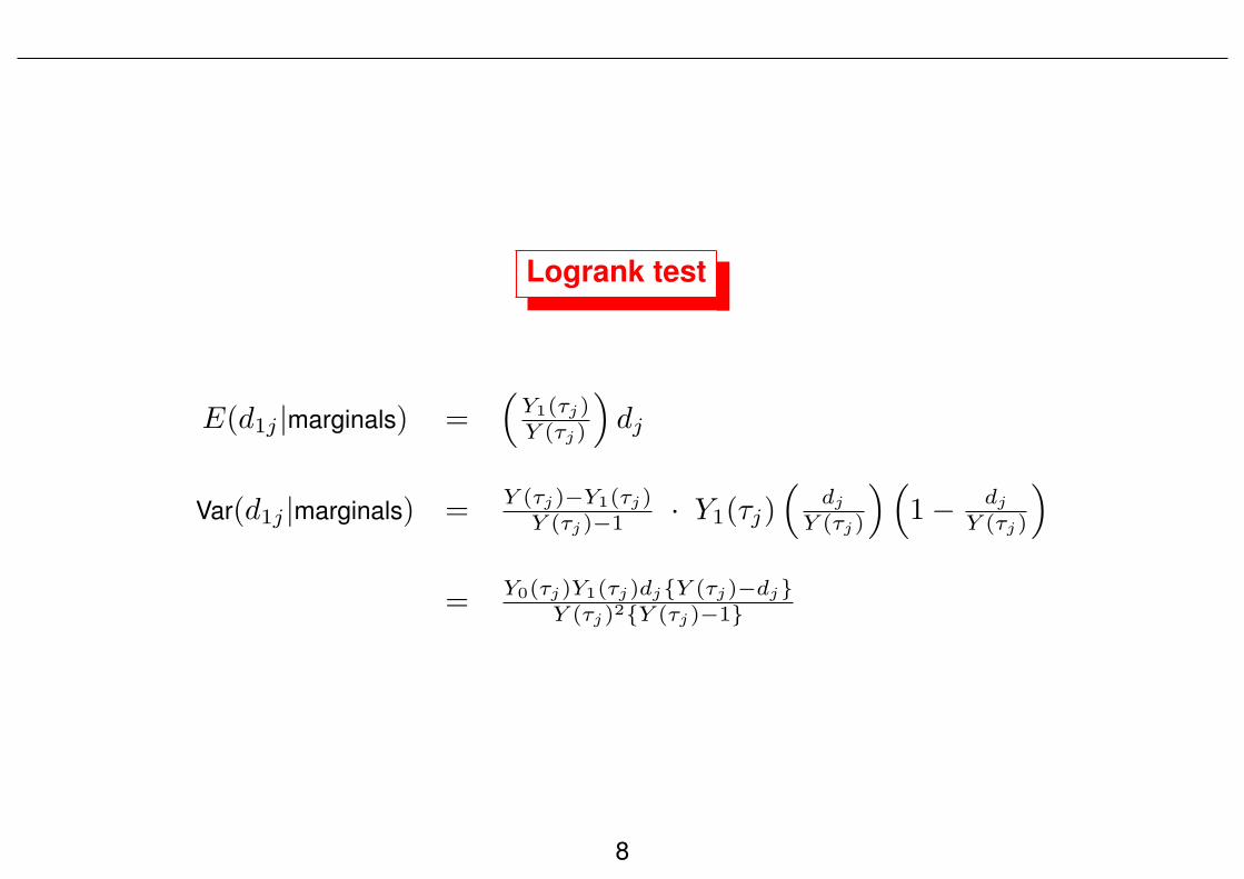
Logrank test
E(d1j |marginals) =(
Y1(τj)Y (τj)
)dj
Var(d1j |marginals) =Y (τj)−Y1(τj)
Y (τj)−1 · Y1(τj)(
dj
Y (τj)
)(1− dj
Y (τj)
)=
Y0(τj)Y1(τj)dj{Y (τj)−dj}Y (τj)2{Y (τj)−1}
8
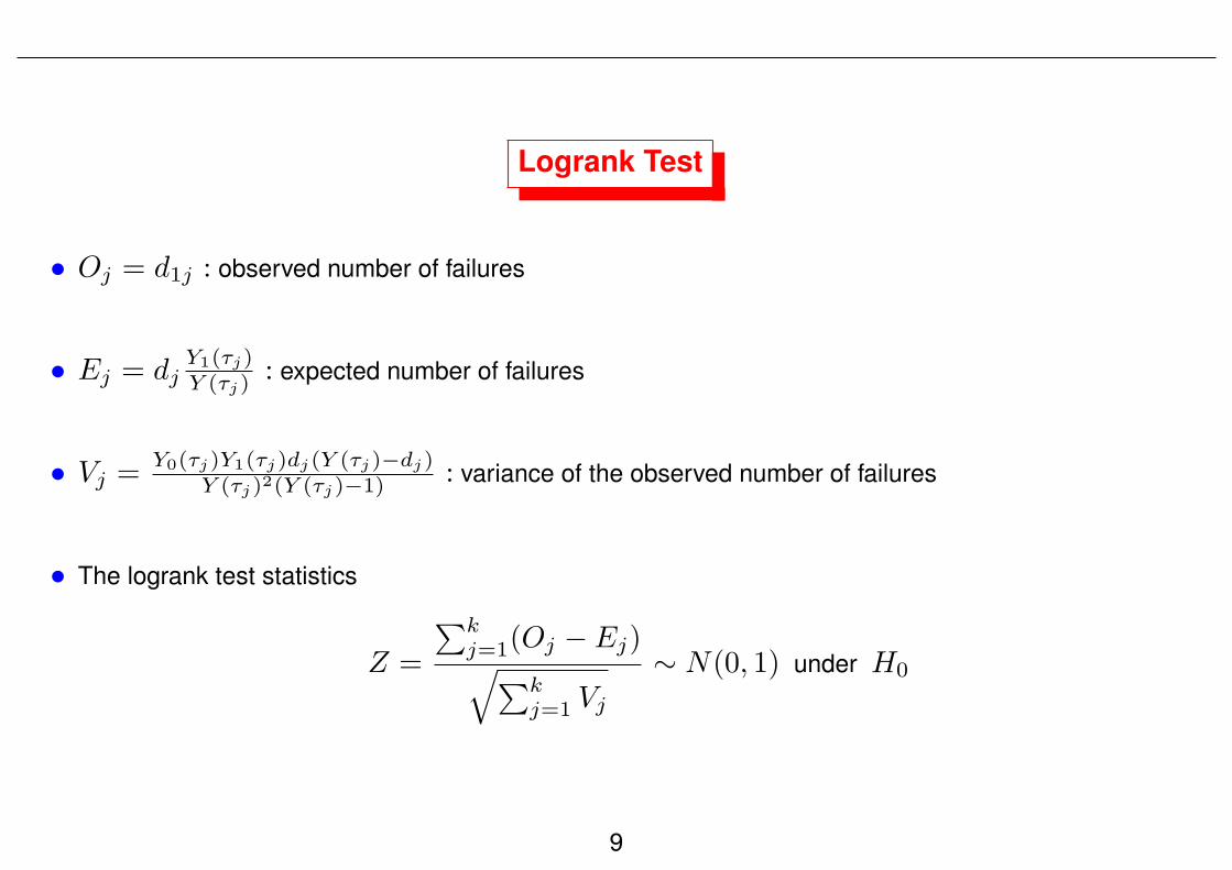
Logrank Test
• Oj = d1j : observed number of failures
• Ej = djY1(τj)Y (τj)
: expected number of failures
• Vj =Y0(τj)Y1(τj)dj(Y (τj)−dj)
Y (τj)2(Y (τj)−1) : variance of the observed number of failures
• The logrank test statistics
Z =
∑kj=1(Oj − Ej)√∑k
j=1 Vj
∼ N(0, 1) under H0
9
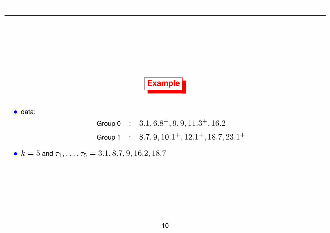
Example
• data:
Group 0 : 3.1, 6.8+, 9, 9, 11.3+, 16.2
Group 1 : 8.7, 9, 10.1+, 12.1+, 18.7, 23.1+
• k = 5 and τ1, . . . , τ5 = 3.1, 8.7, 9, 16.2, 18.7
10
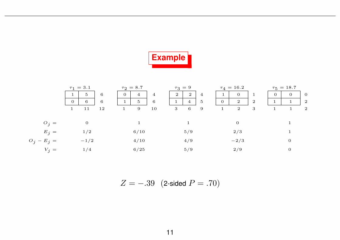
Example
τ1 = 3.1
1 5 6
0 6 6
1 11 12
τ2 = 8.7
0 4 4
1 5 6
1 9 10
τ3 = 9
2 2 4
1 4 5
3 6 9
τ4 = 16.2
1 0 1
0 2 2
1 2 3
τ5 = 18.7
0 0 0
1 1 2
1 1 2
Oj = 0 1 1 0 1
Ej = 1/2 6/10 5/9 2/3 1
Oj − Ej = −1/2 4/10 4/9 −2/3 0
Vj = 1/4 6/25 5/9 2/9 0
Z = −.39 (2-sided P = .70)
11
Logrank test
• Symmetric in two groups
• Only rank matters
• k two by two tables are treated as independent.
• If the number of subjects at risk becomes zero in one group, the additional two by two tables don’t
contribute to the logrank test.
12
Logrank test
• The power of the logrank test depends on the number of observed failures rather than the sample sizes
• Logrank test is most powerful for detecting the alternatives
H1 : S1(t) = S0(t)exp(β) ⇔ h1(t) = h0(t)e
β , β = 0
• The power of logrank test under the alterative h1(t) = h0(t)eβ is approximately
Φ(|β|
√Dπ0(1− π0)− 1.96
),
where D is the expected number of failures and π0 is the proportion of patient in groups 0.
13
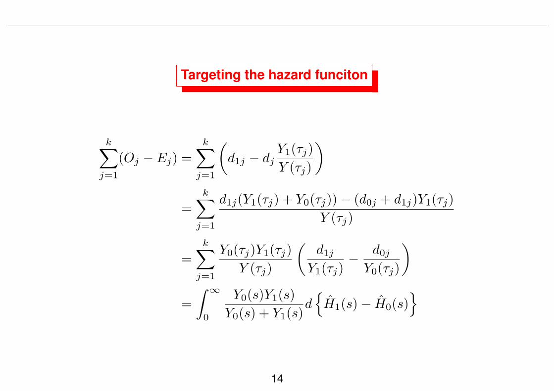
Targeting the hazard funciton
k∑j=1
(Oj − Ej) =k∑
j=1
(d1j − dj
Y1(τj)
Y (τj)
)
=
k∑j=1
d1j(Y1(τj) + Y0(τj))− (d0j + d1j)Y1(τj)
Y (τj)
=
k∑j=1
Y0(τj)Y1(τj)
Y (τj)
(d1j
Y1(τj)− d0j
Y0(τj)
)
=
∫ ∞
0
Y0(s)Y1(s)
Y0(s) + Y1(s)d{H1(s)− H0(s)
}
14
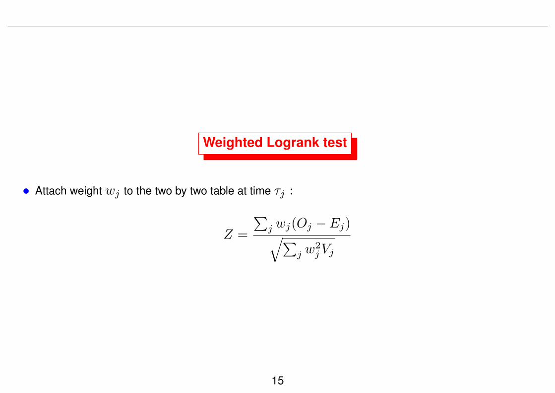
Weighted Logrank test
• Attach weight wj to the two by two table at time τj :
Z =
∑j wj(Oj − Ej)√∑
j w2jVj
15
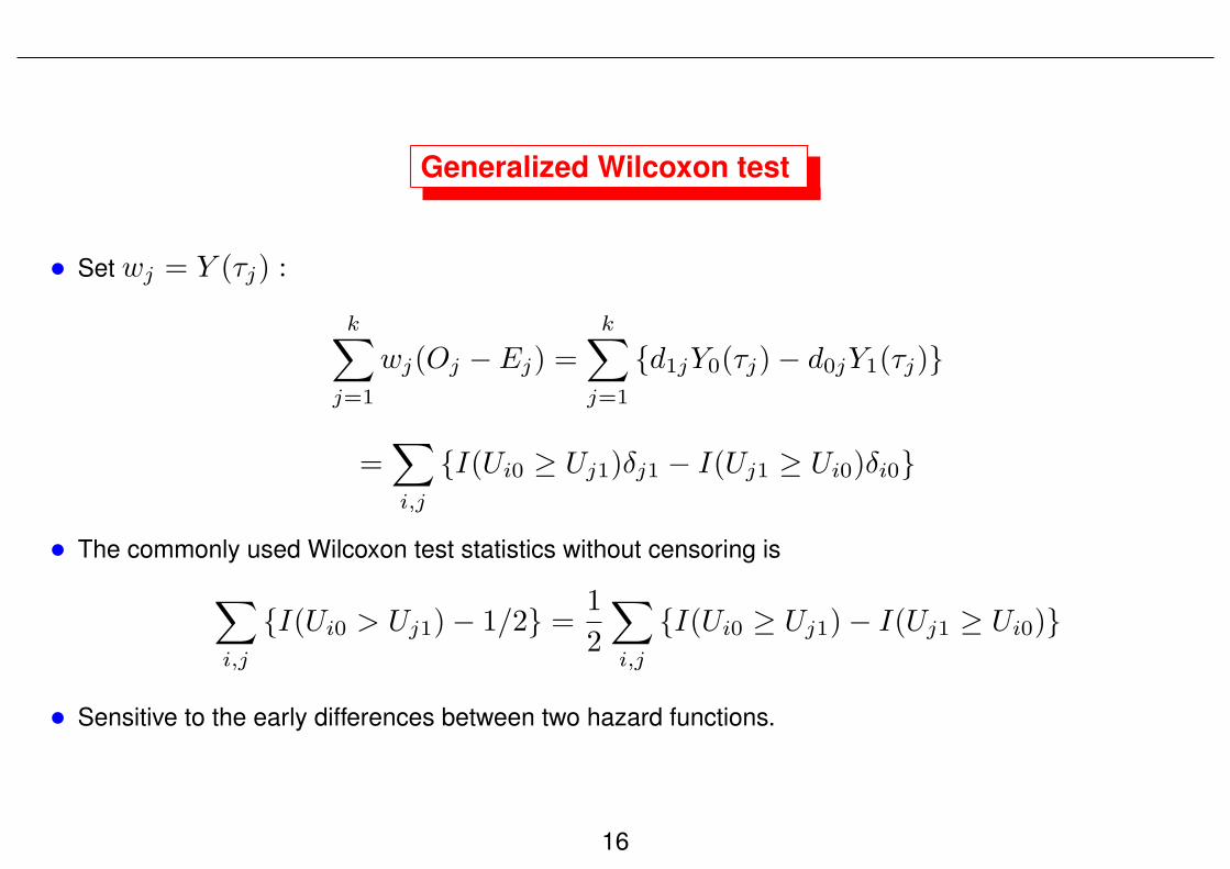
Generalized Wilcoxon test
• Set wj = Y (τj) :
k∑j=1
wj(Oj − Ej) =k∑
j=1
{d1jY0(τj)− d0jY1(τj)}
=∑i,j
{I(Ui0 ≥ Uj1)δj1 − I(Uj1 ≥ Ui0)δi0}
• The commonly used Wilcoxon test statistics without censoring is∑i,j
{I(Ui0 > Uj1)− 1/2} =1
2
∑i,j
{I(Ui0 ≥ Uj1)− I(Uj1 ≥ Ui0)}
• Sensitive to the early differences between two hazard functions.
16

The Generalized Logrank test
• In general, the test statistics is in the form of
Zw =
∫ τ
0w(s)d
{H1(s)− H0(s)
}σw
• The choice of the weight affects the power.
• One may construct a test based on several different sets of weights, e.g.,
T = max{|Zw1|, |Zw2
|, · · · , |ZwL|}.
17
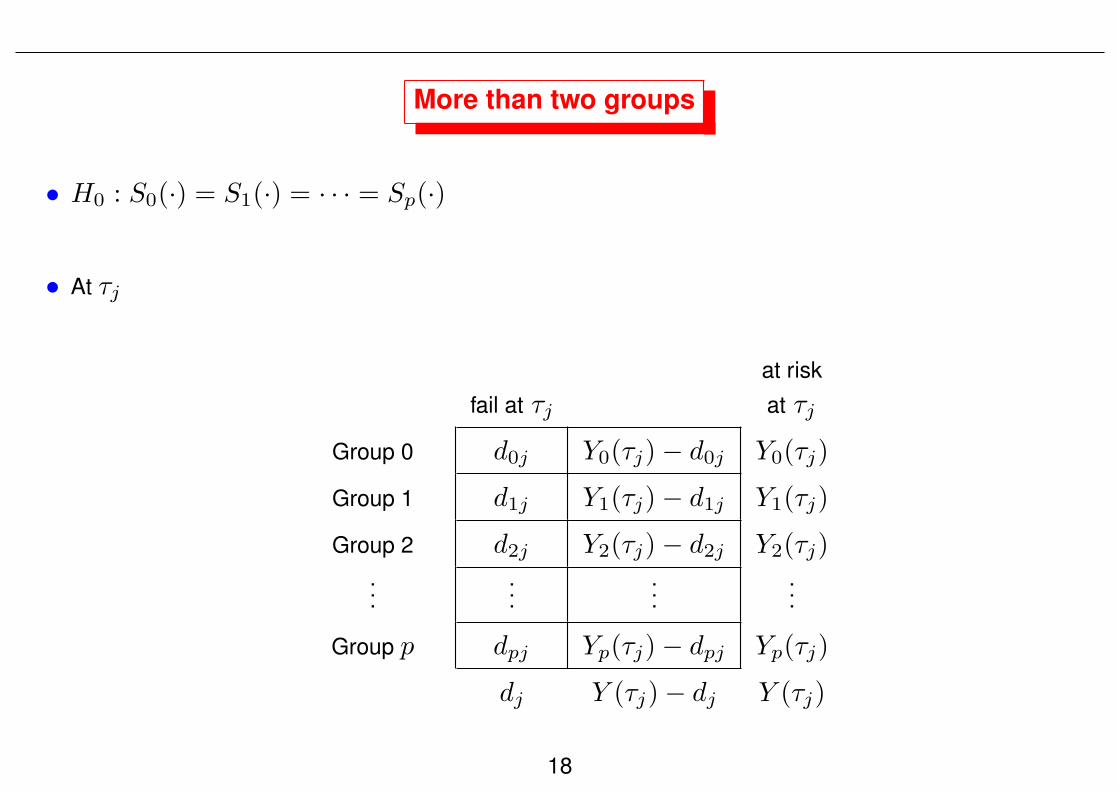
More than two groups
• H0 : S0(·) = S1(·) = · · · = Sp(·)
• At τj
at risk
fail at τj at τj
Group 0 d0j Y0(τj)− d0j Y0(τj)
Group 1 d1j Y1(τj)− d1j Y1(τj)
Group 2 d2j Y2(τj)− d2j Y2(τj)...
......
...
Group p dpj Yp(τj)− dpj Yp(τj)
dj Y (τj)− dj Y (τj)
18
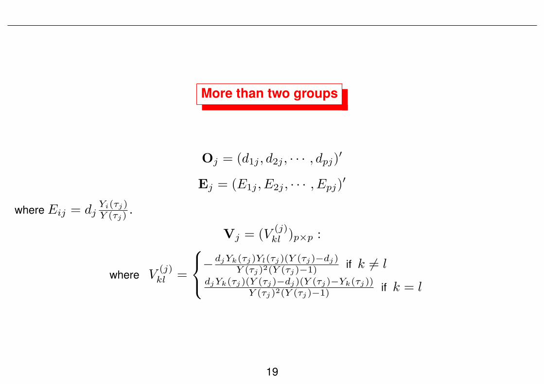
More than two groups
Oj = (d1j , d2j , · · · , dpj)′
Ej = (E1j , E2j , · · · , Epj)′
where Eij = djYi(τj)Y (τj)
.
Vj = (V(j)kl )p×p :
where V(j)kl =
−djYk(τj)Yl(τj)(Y (τj)−dj)Y (τj)2(Y (τj)−1) if k = l
djYk(τj)(Y (τj)−dj)(Y (τj)−Yk(τj))Y (τj)2(Y (τj)−1) if k = l
19
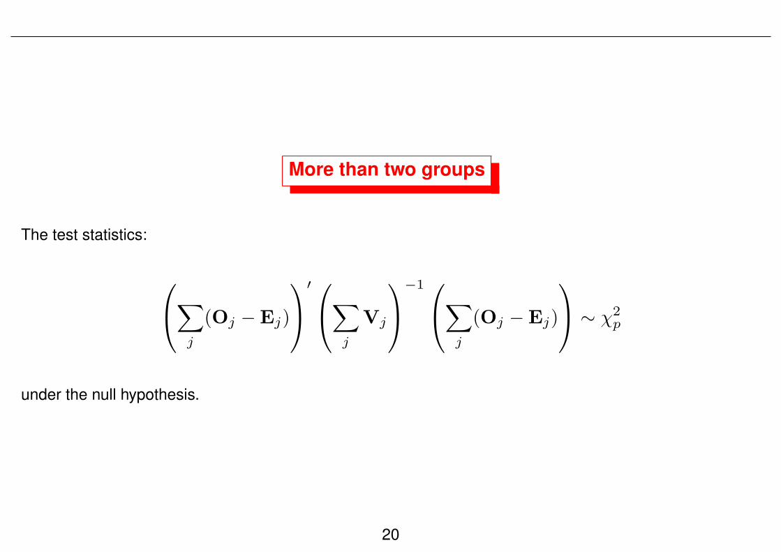
More than two groups
The test statistics:
∑j
(Oj −Ej)
′ ∑j
Vj
−1 ∑j
(Oj −Ej)
∼ χ2p
under the null hypothesis.
20

More than two groups
Trend test
∑j c
′(Oj −Ej)√∑j c
′Vjc∼ N(0, 1)
under the null hypothesis. How to choose the vector c to increase the power?
21
Related Documents