SURVIVAL ANALYSIS By Danielle Walkup Cyrenea Piper And Thomas Huff

Welcome message from author
This document is posted to help you gain knowledge. Please leave a comment to let me know what you think about it! Share it to your friends and learn new things together.
Transcript

SURVIVAL ANALYSIS
By
Danielle Walkup
Cyrenea Piper
And Thomas Huff
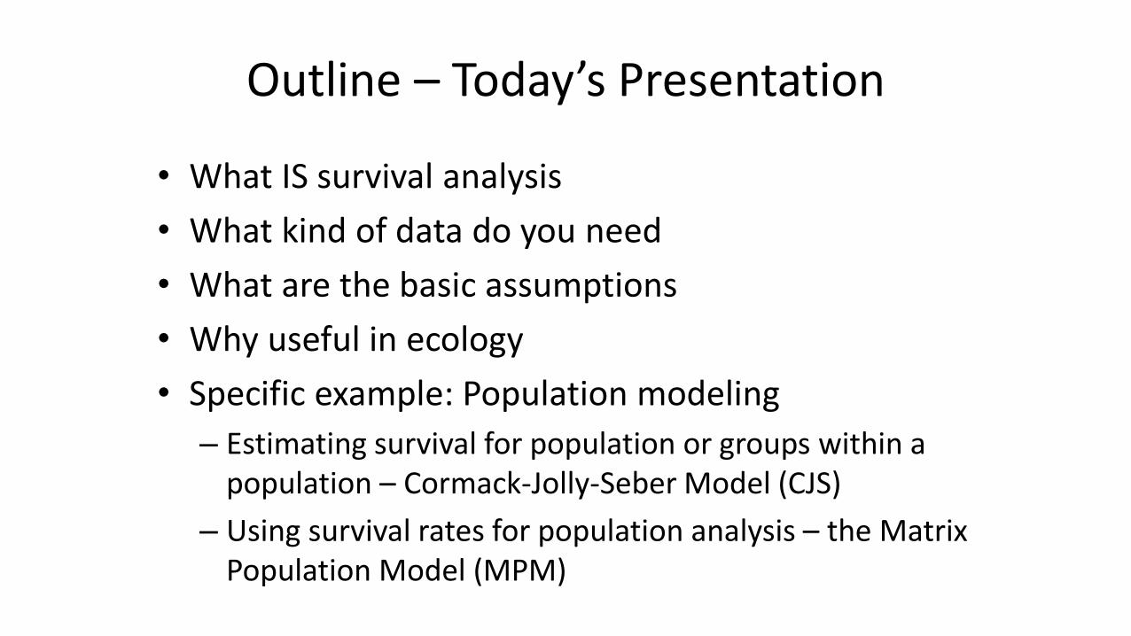
Outline – Today’s Presentation
• What IS survival analysis
• What kind of data do you need
• What are the basic assumptions
• Why useful in ecology
• Specific example: Population modeling
– Estimating survival for population or groups within a population – Cormack-Jolly-Seber Model (CJS)
– Using survival rates for population analysis – the Matrix Population Model (MPM)
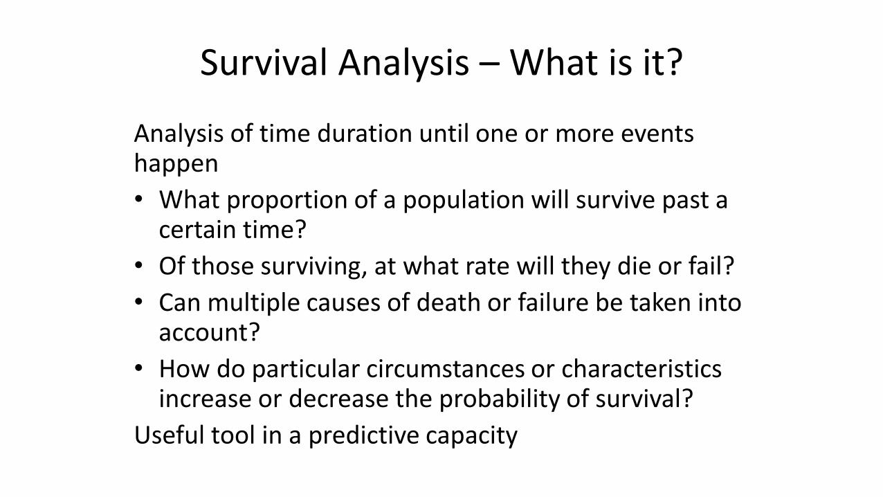
Survival Analysis – What is it?
Analysis of time duration until one or more events happen
• What proportion of a population will survive past a certain time?
• Of those surviving, at what rate will they die or fail?
• Can multiple causes of death or failure be taken into account?
• How do particular circumstances or characteristics increase or decrease the probability of survival?
Useful tool in a predictive capacity
Survival Analysis - Aliases
• Reliability Theory/Reliability Analysis - Engineering
• Duration Analysis/Duration Modeling - Economics
• Event History Analysis - Sociology
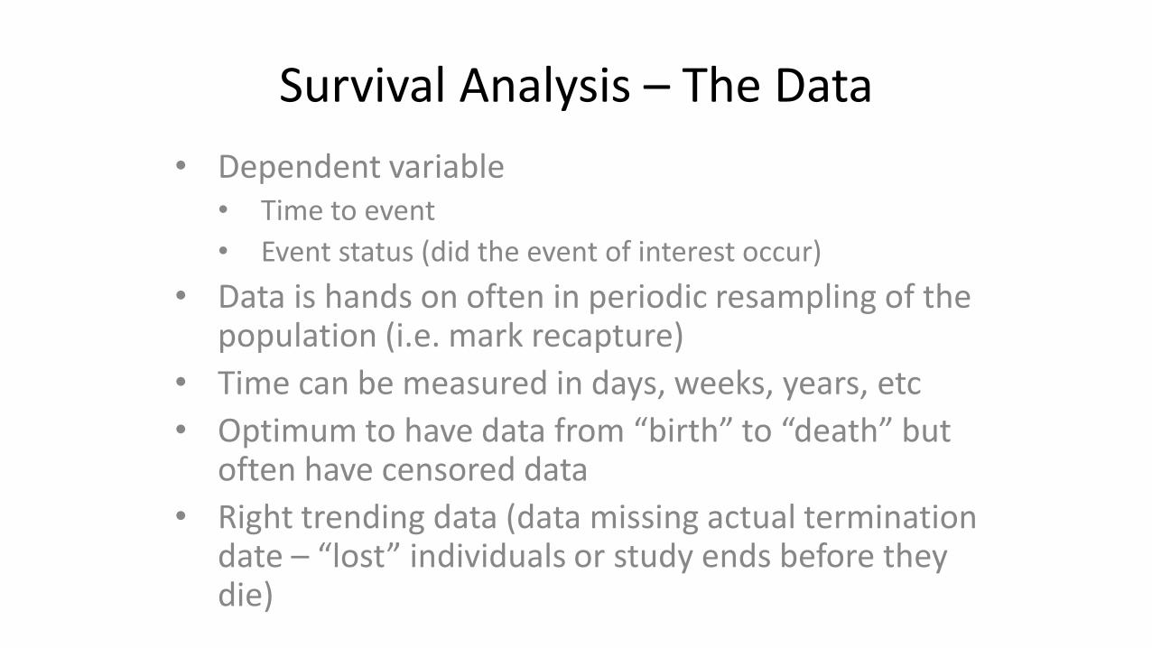
Survival Analysis – The Data
• Dependent variable• Time to event
• Event status (did the event of interest occur)
• Data is hands on often in periodic resampling of the population (i.e. mark recapture)
• Time can be measured in days, weeks, years, etc
• Optimum to have data from “birth” to “death” but often have censored data
• Right trending data (data missing actual termination date – “lost” individuals or study ends before they die)
Survival Analysis – what it does
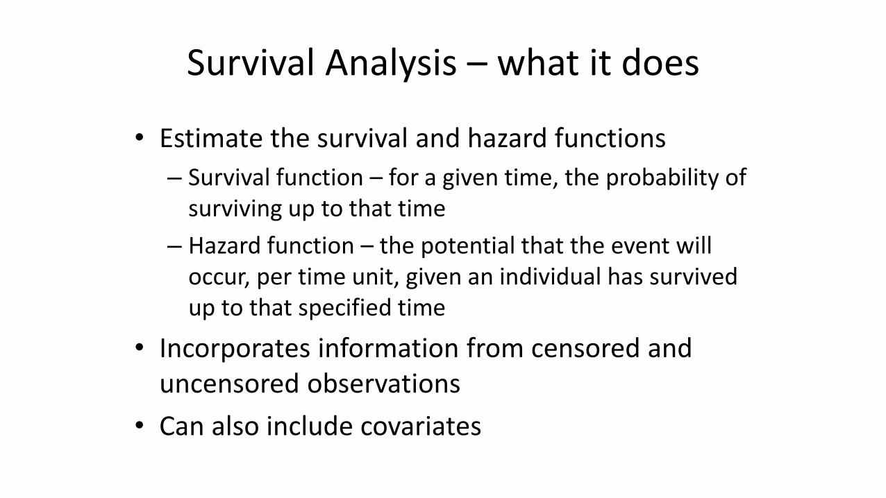
• Estimate the survival and hazard functions
– Survival function – for a given time, the probability of surviving up to that time
– Hazard function – the potential that the event will occur, per time unit, given an individual has survived up to that specified time
• Incorporates information from censored and uncensored observations
• Can also include covariates
Survival Analysis - Approaches
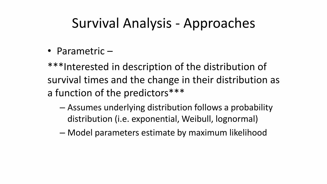
• Parametric –
***Interested in description of the distribution of survival times and the change in their distribution as a function of the predictors***
– Assumes underlying distribution follows a probability distribution (i.e. exponential, Weibull, lognormal)
– Model parameters estimate by maximum likelihood
Survival Analysis - Approaches
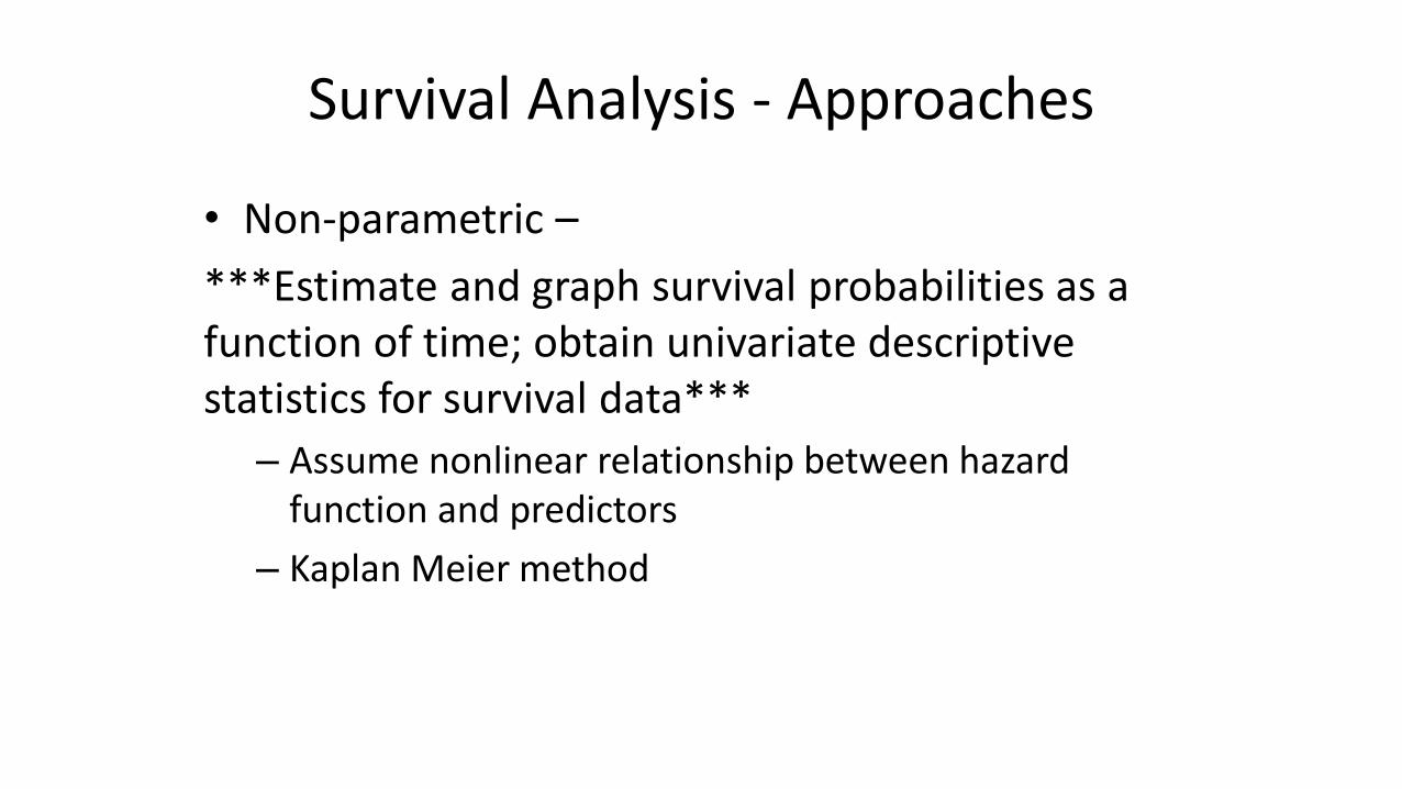
• Non-parametric –
***Estimate and graph survival probabilities as a function of time; obtain univariate descriptive statistics for survival data***
– Assume nonlinear relationship between hazard function and predictors
– Kaplan Meier method
Survival Analysis - Approaches
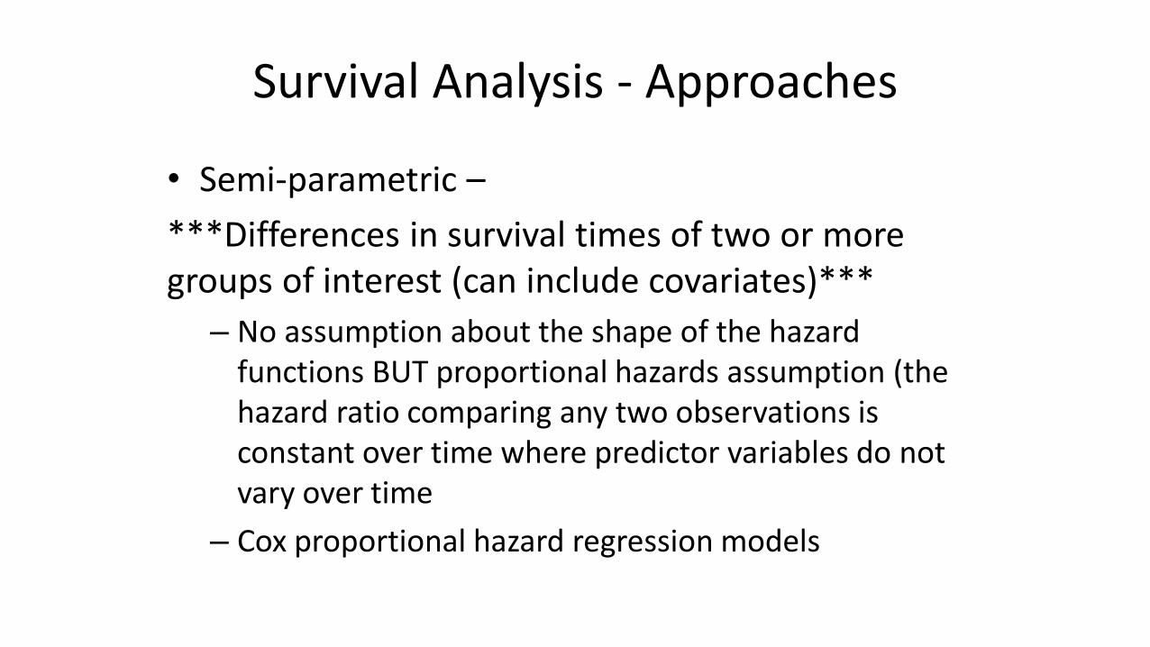
• Semi-parametric –
***Differences in survival times of two or more groups of interest (can include covariates)***
– No assumption about the shape of the hazard functions BUT proportional hazards assumption (the hazard ratio comparing any two observations is constant over time where predictor variables do not vary over time
– Cox proportional hazard regression models
Survival Analysis - Examples
For more on Survival Analysis and Hazard Functions see:
http://rpubs.com/daspringate/survival
www.ms.uky.edu/~mai/Rsurv.pdf
www.stat.ucdavis.edu/.../R_tutorial
Example from Ecology
What will happen to a population in the long term?
– One form of survival analysis using Capture-Recapture methods
– Using estimated survival rates along with reproduction rates in Matrix Population Models
Capture Mark Recapture Methods
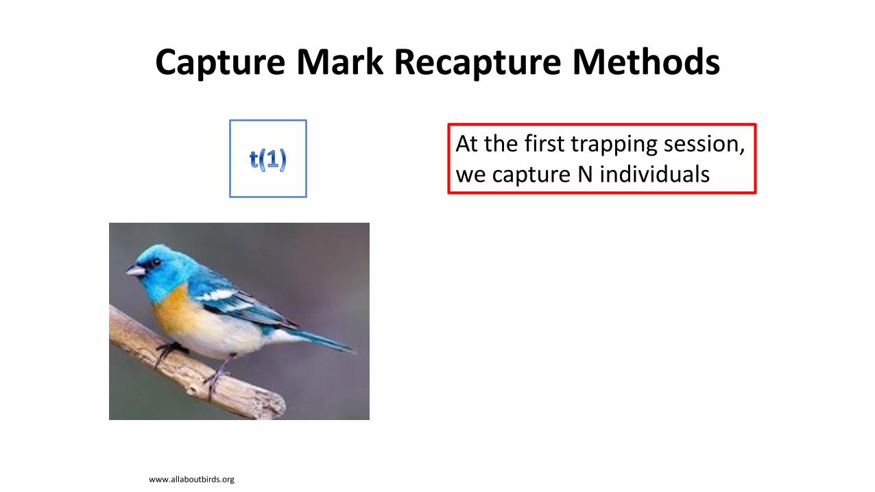
At the first trapping session, we capture N individuals
www.allaboutbirds.org

Capture Mark Recapture Methods
And assign individuals unique, permanent marks
www.allaboutbirds.org ; www.rrbo.org
Capture Mark Recapture Methods
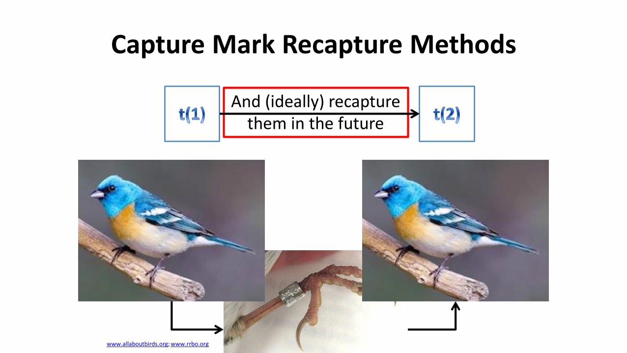
And (ideally) recapture them in the future
www.allaboutbirds.org; www.rrbo.org
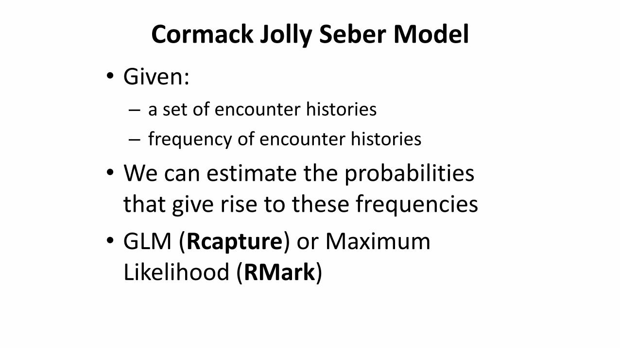
Cormack Jolly Seber Model
• Given:– a set of encounter histories
– frequency of encounter histories
• We can estimate the probabilities that give rise to these frequencies
• GLM (Rcapture) or Maximum Likelihood (RMark)
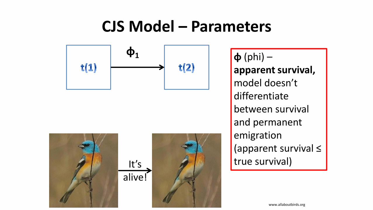
CJS Model – Parameters
φ1 φ (phi) –apparent survival,model doesn’t differentiate between survival and permanent emigration (apparent survival ≤ true survival)It’s
alive!
www.allaboutbirds.org
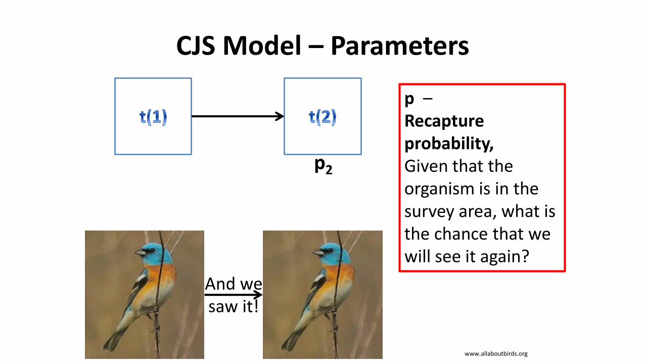
CJS Model – Parameters
p2
p –Recapture probability,Given that the organism is in the survey area, what is the chance that we will see it again?
And we saw it!
www.allaboutbirds.org
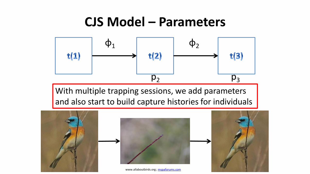
CJS Model – Parameters
φ1 φ2
p2 p3
With multiple trapping sessions, we add parameters and also start to build capture histories for individuals
www.allaboutbirds.org ; mspaforums.com

CJS - Assumptions
However there are a few things we need to be aware of when working with these models.
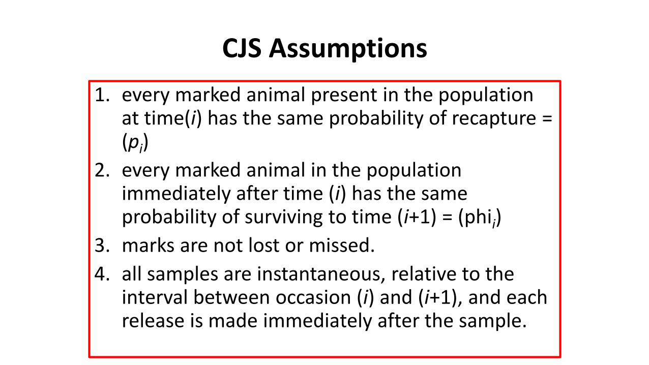
CJS Assumptions
1. every marked animal present in the population at time(i) has the same probability of recapture = (pi)
2. every marked animal in the population immediately after time (i) has the same probability of surviving to time (i+1) = (phii)
3. marks are not lost or missed.
4. all samples are instantaneous, relative to the interval between occasion (i) and (i+1), and each release is made immediately after the sample.
In practice, we know that most animal populations aren’t that easy to constrain and so numerous
models have been developed to account for unmet assumptions and various modeling issues
encountered
CJS – You know what they say about when you assume…
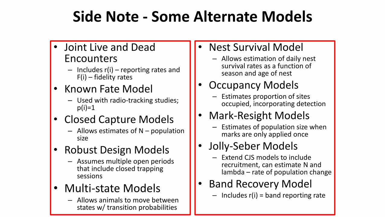
Side Note - Some Alternate Models
• Joint Live and Dead Encounters– Includes r(i) – reporting rates and
F(i) – fidelity rates
• Known Fate Model– Used with radio-tracking studies;
p(i)=1
• Closed Capture Models– Allows estimates of N – population
size
• Robust Design Models– Assumes multiple open periods
that include closed trapping sessions
• Multi-state Models– Allows animals to move between
states w/ transition probabilities
• Nest Survival Model– Allows estimation of daily nest
survival rates as a function of season and age of nest
• Occupancy Models– Estimates proportion of sites
occupied, incorporating detection
• Mark-Resight Models– Estimates of population size when
marks are only applied once
• Jolly-Seber Models– Extend CJS models to include
recruitment, can estimate N and lambda – rate of population change
• Band Recovery Model– Includes r(i) = band reporting rate
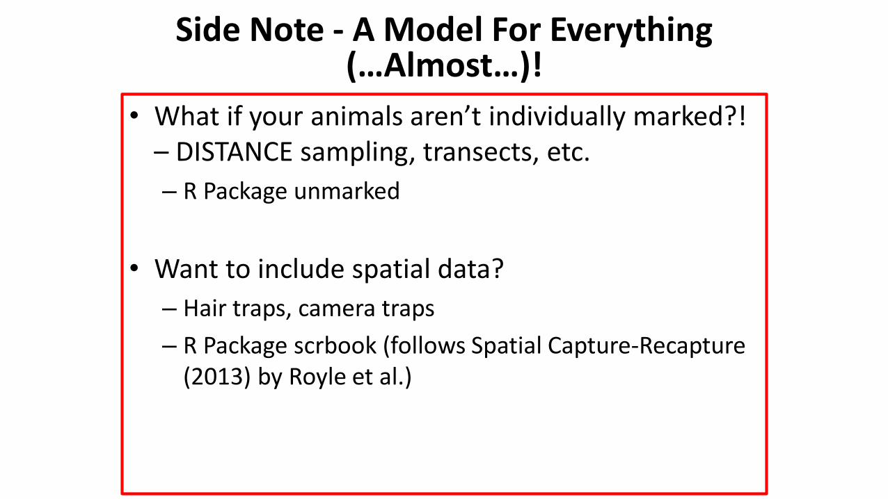
Side Note - A Model For Everything (…Almost…)!
• What if your animals aren’t individually marked?! – DISTANCE sampling, transects, etc.
– R Package unmarked
• Want to include spatial data?
– Hair traps, camera traps
– R Package scrbook (follows Spatial Capture-Recapture (2013) by Royle et al.)
CJS Model – Building Encounter Histories
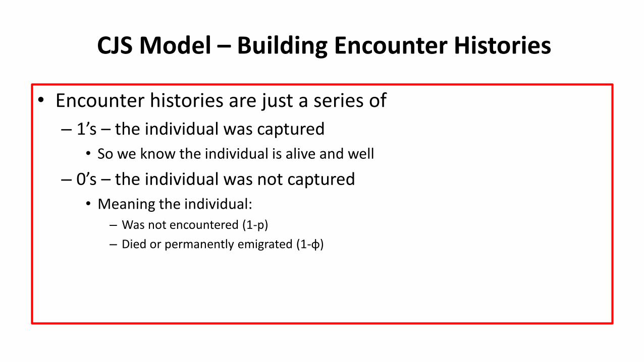
• Encounter histories are just a series of
– 1’s – the individual was captured
• So we know the individual is alive and well
– 0’s – the individual was not captured
• Meaning the individual:– Was not encountered (1-p)
– Died or permanently emigrated (1-φ)
CJS Model – Building Encounter Histories
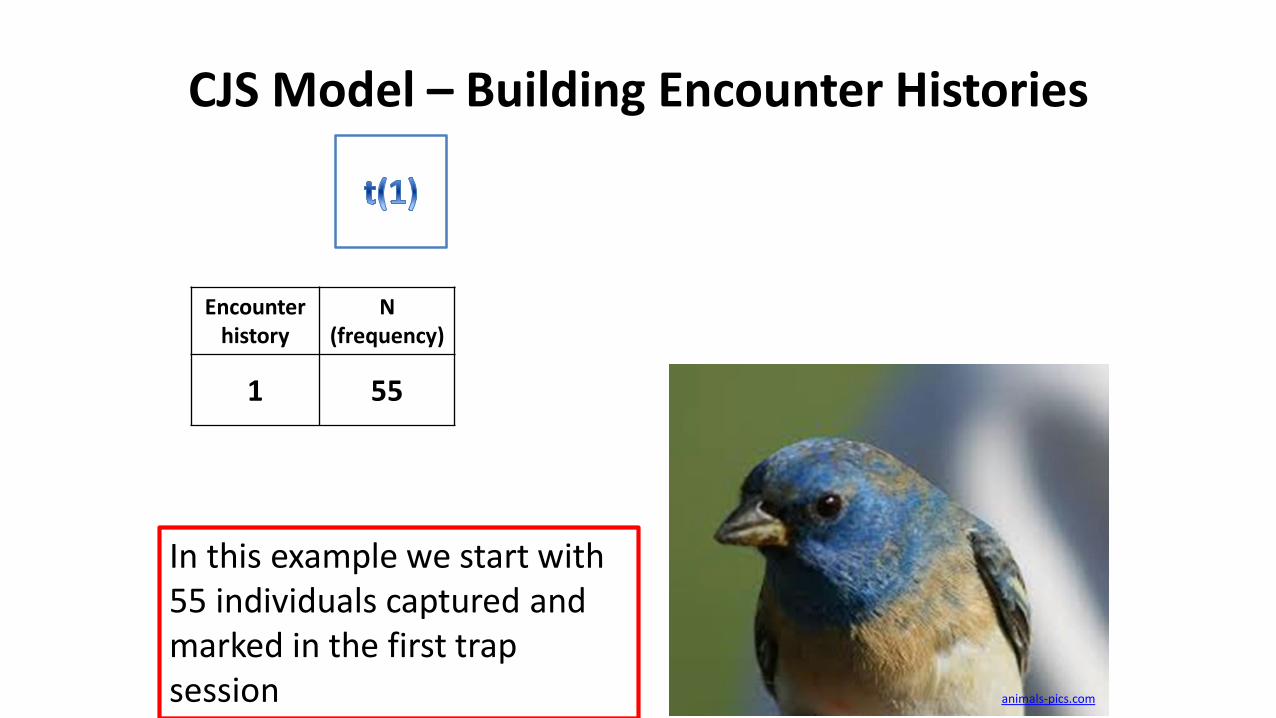
Encounter history
N(frequency)
1 55
In this example we start with 55 individuals captured and marked in the first trap session animals-pics.com
CJS Model – Building Encounter Histories
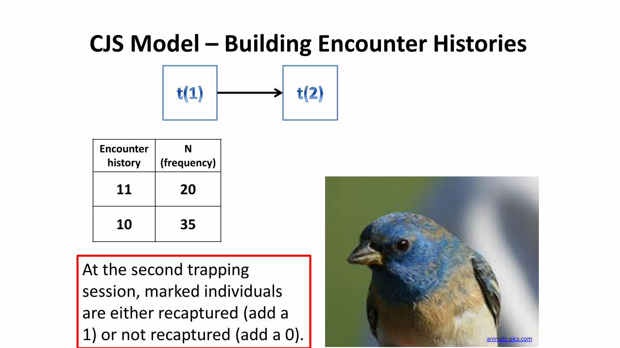
Encounter history
N(frequency)
11 20
10 35
At the second trapping session, marked individuals are either recaptured (add a 1) or not recaptured (add a 0). animals-pics.com
CJS Model – Building Encounter Histories
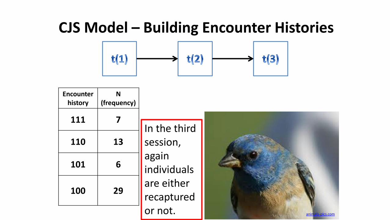
Encounter history
N(frequency)
111 7
110 13
101 6
100 29
In the third session, again individuals are either recaptured or not. animals-pics.com
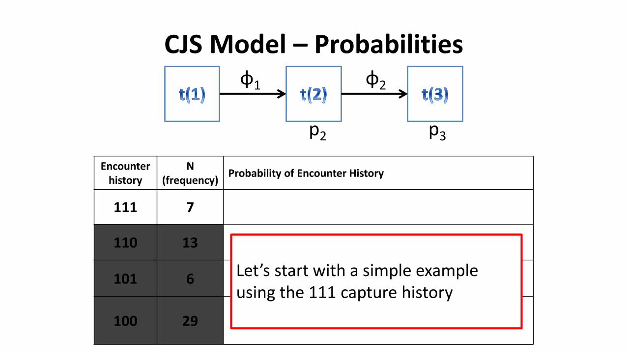
CJS Model – Probabilities
Encounter history
N(frequency)
Probability of Encounter History
111 7
110 13
101 6
100 29
φ1 φ2
p2 p3
Let’s start with a simple example using the 111 capture history

CJS Model – Encounter Histories?!
Encounter history
N(frequency)
Probability of Encounter History
111 7 φ1
110 13
101 6
100 29
φ1 φ2
p2 p3
Individuals survive from time 1 to time 2 – start with φ1
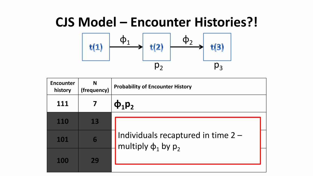
CJS Model – Encounter Histories?!
Encounter history
N(frequency)
Probability of Encounter History
111 7 φ1p2
110 13
101 6
100 29
φ1 φ2
p2 p3
Individuals recaptured in time 2 –multiply φ1 by p2

CJS Model – Encounter Histories?!
Encounter history
N(frequency)
Probability of Encounter History
111 7 φ1p2φ2
110 13
101 6
100 29
φ1 φ2
p2 p3
Individuals survive from time 2 to time 3 – multiply φ1p2 by φ2

CJS Model – Encounter Histories?!
Encounter history
N(frequency)
Probability of Encounter History
111 7 φ1p2φ2p3
110 13
101 6
100 29
φ1 φ2
p2 p3
Individuals recaptured in time 3 –multiply φ1p2φ2 by p3
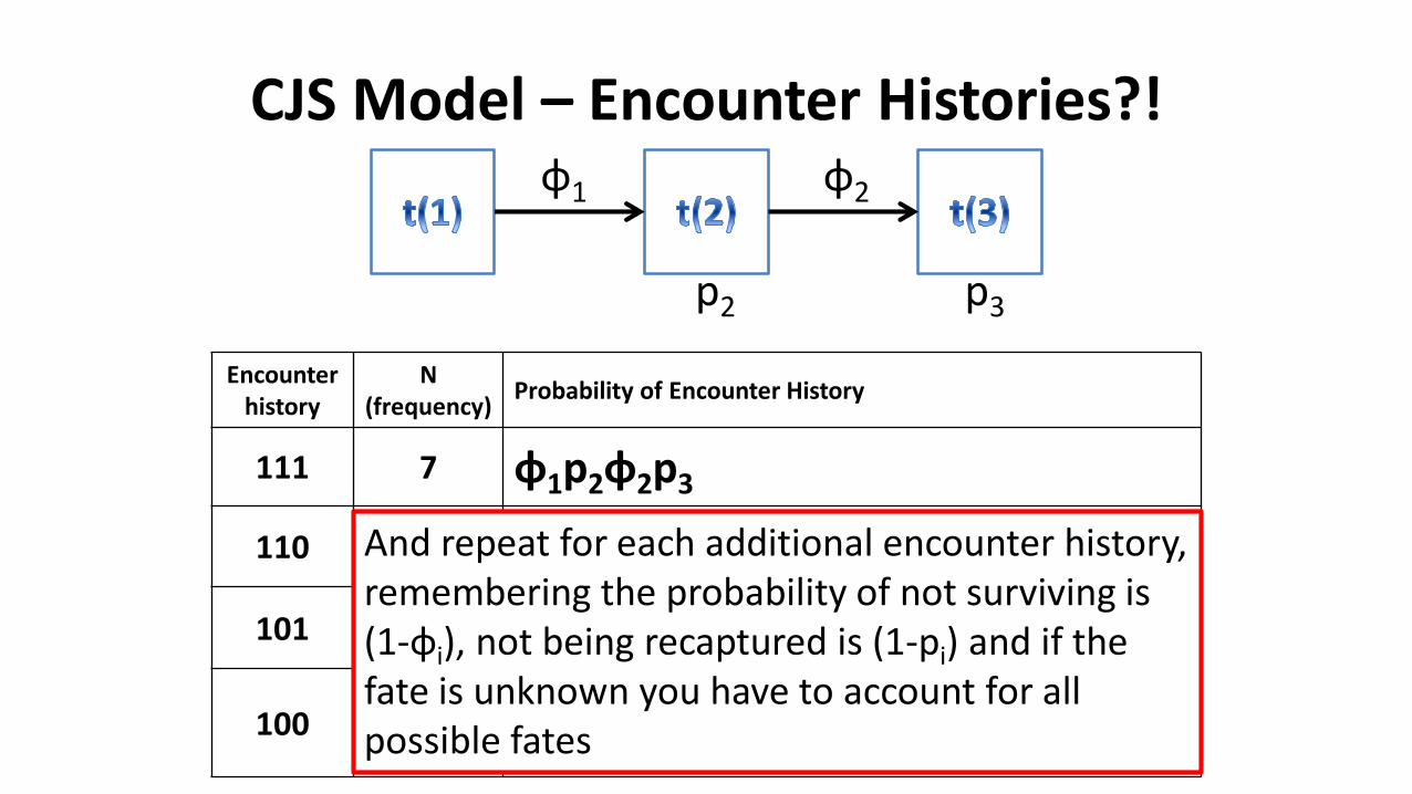
CJS Model – Encounter Histories?!
Encounter history
N(frequency)
Probability of Encounter History
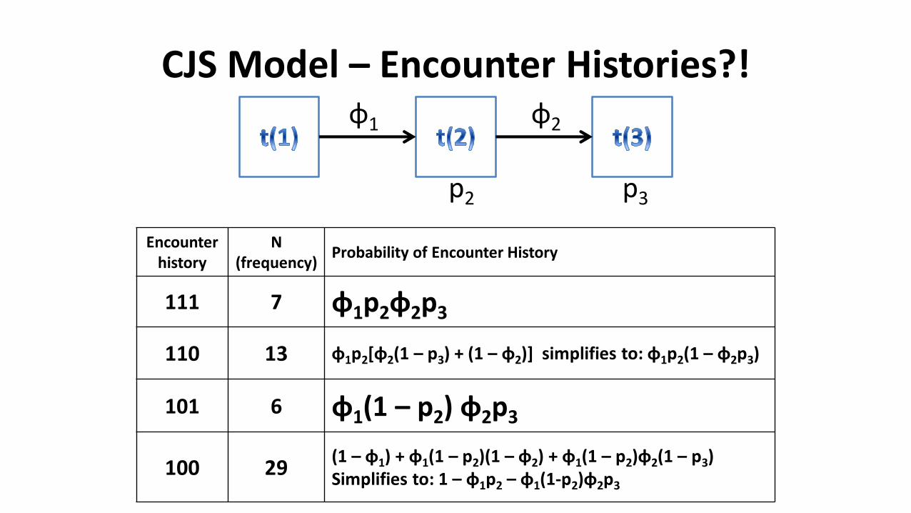
111 7 φ1p2φ2p3
110 13 φ1p2[φ2(1 – p3) + (1 – φ2)] simplifies to: φ1p2(1 – φ2p3)
101 6 φ1(1 – p2) φ2p3
100 29(1 – φ1) + φ1(1 – p2)(1 – φ2) + φ1(1 – p2)φ2(1 – p3)Simplifies to: 1 – φ1p2 – φ1(1-p2)φ2p3
φ1 φ2
p2 p3
And repeat for each additional encounter history, remembering the probability of not surviving is (1-φi), not being recaptured is (1-pi) and if the fate is unknown you have to account for all possible fates
CJS Model – Encounter Histories?!
Encounter history
N(frequency)
Probability of Encounter History
111 7 φ1p2φ2p3
110 13 φ1p2[φ2(1 – p3) + (1 – φ2)] simplifies to: φ1p2(1 – φ2p3)
101 6 φ1(1 – p2) φ2p3
100 29(1 – φ1) + φ1(1 – p2)(1 – φ2) + φ1(1 – p2)φ2(1 – p3)Simplifies to: 1 – φ1p2 – φ1(1-p2)φ2p3
φ1 φ2
p2 p3
CJS – Maximum Likelihoods
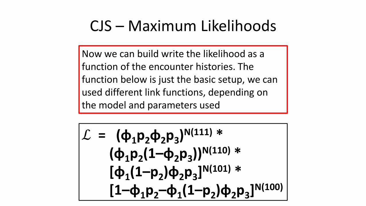
ℒ = (φ1p2φ2p3)N(111) * (φ1p2(1–φ2p3))N(110) *[φ1(1–p2)φ2p3]N(101) * [1–φ1p2–φ1(1–p2)φ2p3]N(100)
Now we can build write the likelihood as a function of the encounter histories. The function below is just the basic setup, we can used different link functions, depending on the model and parameters used
CJS – Maximum Likelihoods
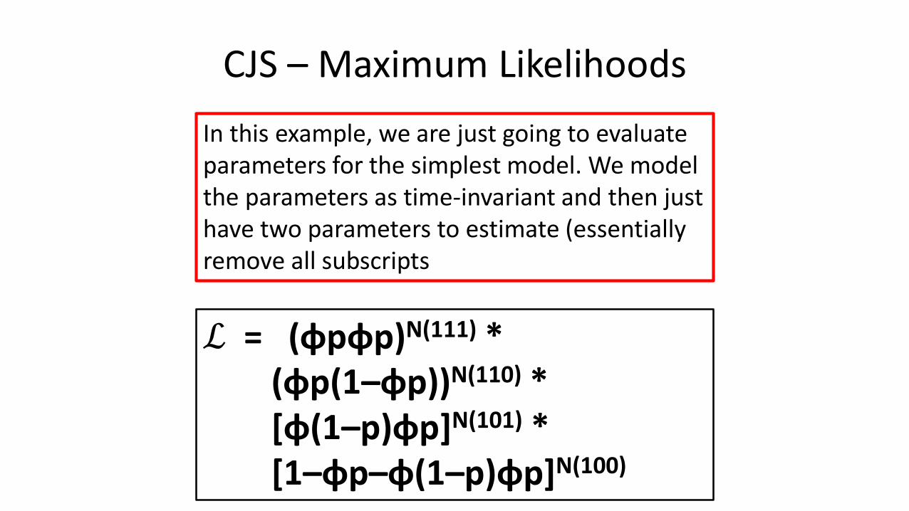
ℒ = (φpφp)N(111) * (φp(1–φp))N(110) *[φ(1–p)φp]N(101) * [1–φp–φ(1–p)φp]N(100)
In this example, we are just going to evaluate parameters for the simplest model. We model the parameters as time-invariant and then just have two parameters to estimate (essentially remove all subscripts
CJS – Maximum Likelihood
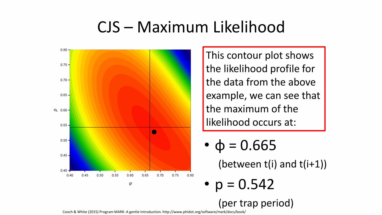
• φ = 0.665 (between t(i) and t(i+1))
• p = 0.542 (per trap period)
This contour plot shows the likelihood profile for the data from the above example, we can see that the maximum of the likelihood occurs at:
Cooch & White (2015) Program MARK: A gentle Introduction. http://www.phidot.org/software/mark/docs/book/
CJS – Discussion
The above problem could be solved analytically relatively easily, however most are not that simple, so programs like MARK solve these likelihoods
numerically (as seen in the plot above)
CJS – Discussion
We can further explore time dependent models, or models that
divide the individuals by groups (sex, cohort, etc.) or add individual
covariates (length, mass, etc.) in the case of heterogeneity in the
population that could lead to differences in survival rates
CJS – Survival Probabilities
So now we have our estimate for survival – what do we do now?!
One option is using survival estimates (and other vital rates) in a Matrix Population Models
www.sandiegobirding.com; www.dosavannah.com
CMR & CJS References
• Lebreton et al. 1992. Modeling survival and testing biological hypothesis using marked animals: a unified approach with case studies. Ecological Monographs 62(1): 67-118.
• Cooch & White. 2015. Program MARK: a gentle introduction. 14th ed. http://www.phidot.org/software/mark/docs/book/
• Laake, J.L. (2013). RMark: An R Interface for Analysis of Capture-Recapture Data with MARK. AFSC Processed Rep 2013-01, 25p.
• Louis-Paul Rivest and Sophie Baillargeon (2014). Rcapture: Loglinear Models for Capture-Recapture Experiments. R package version 1.4-2. http://CRAN.R-project.org/package=Rcapture
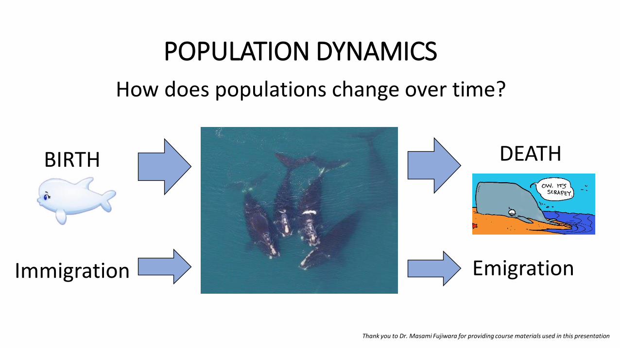
POPULATION DYNAMICS
How does populations change over time?
Thank you to Dr. Masami Fujiwara for providing course materials used in this presentation
BIRTH
Immigration Emigration
DEATH
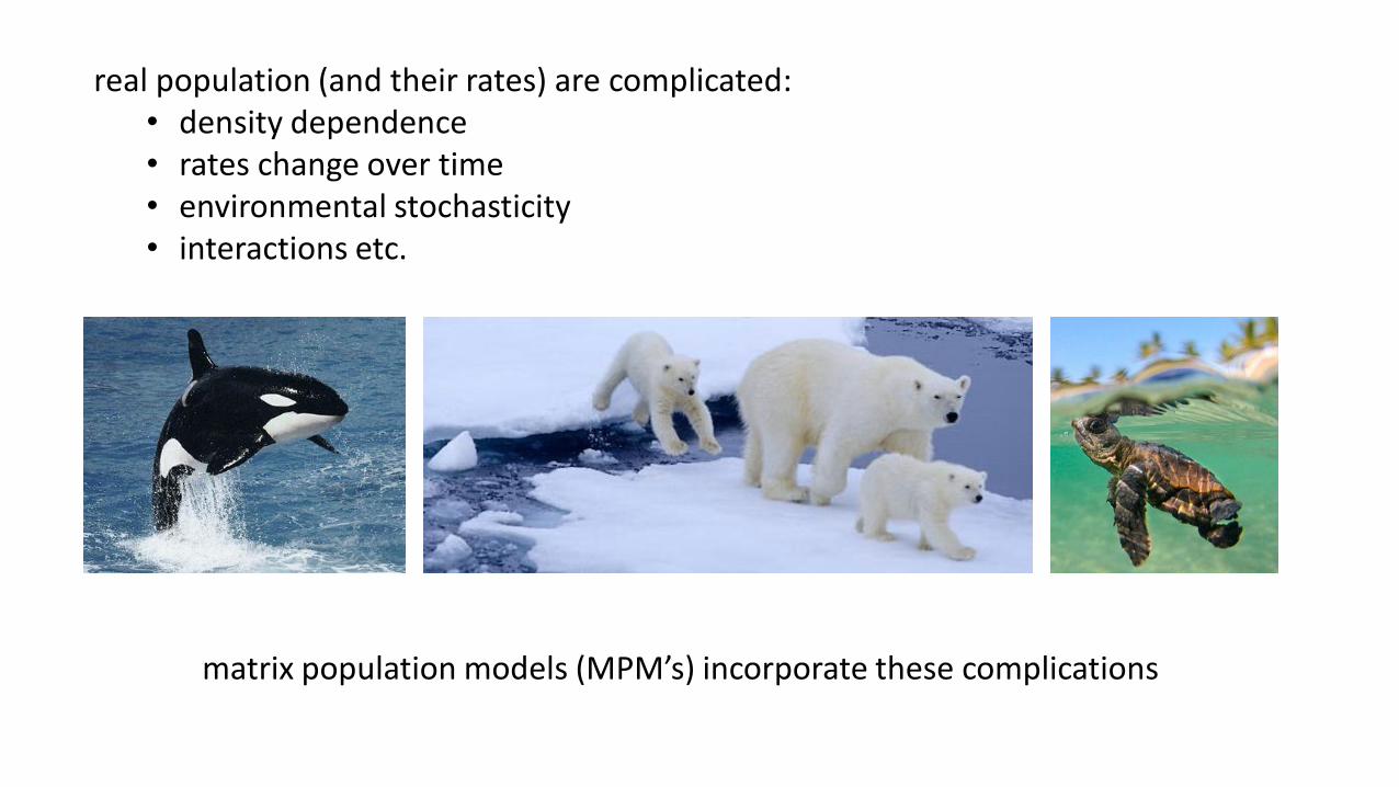
real population (and their rates) are complicated:• density dependence• rates change over time• environmental stochasticity• interactions etc.
matrix population models (MPM’s) incorporate these complications
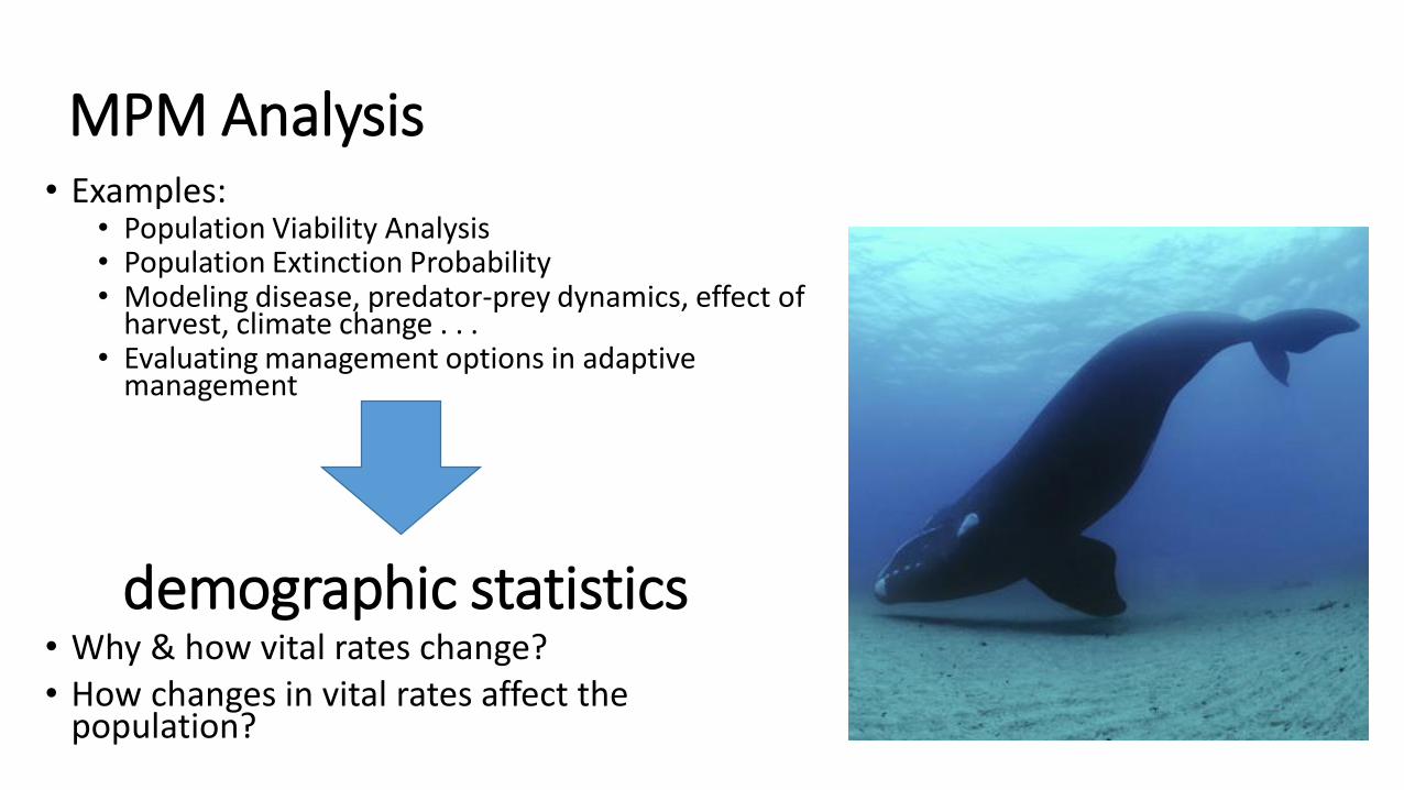
• Examples:• Population Viability Analysis • Population Extinction Probability • Modeling disease, predator-prey dynamics, effect of
harvest, climate change . . . • Evaluating management options in adaptive
management
• Why & how vital rates change?• How changes in vital rates affect the
population?
MPM Analysis
demographic statistics
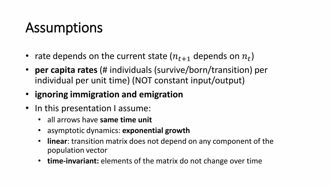
Assumptions
• rate depends on the current state (𝑛𝑡+1 depends on 𝑛𝑡)
• per capita rates (# individuals (survive/born/transition) per individual per unit time) (NOT constant input/output)
• ignoring immigration and emigration
• In this presentation I assume:• all arrows have same time unit
• asymptotic dynamics: exponential growth
• linear: transition matrix does not depend on any component of the population vector
• time-invariant: elements of the matrix do not change over time
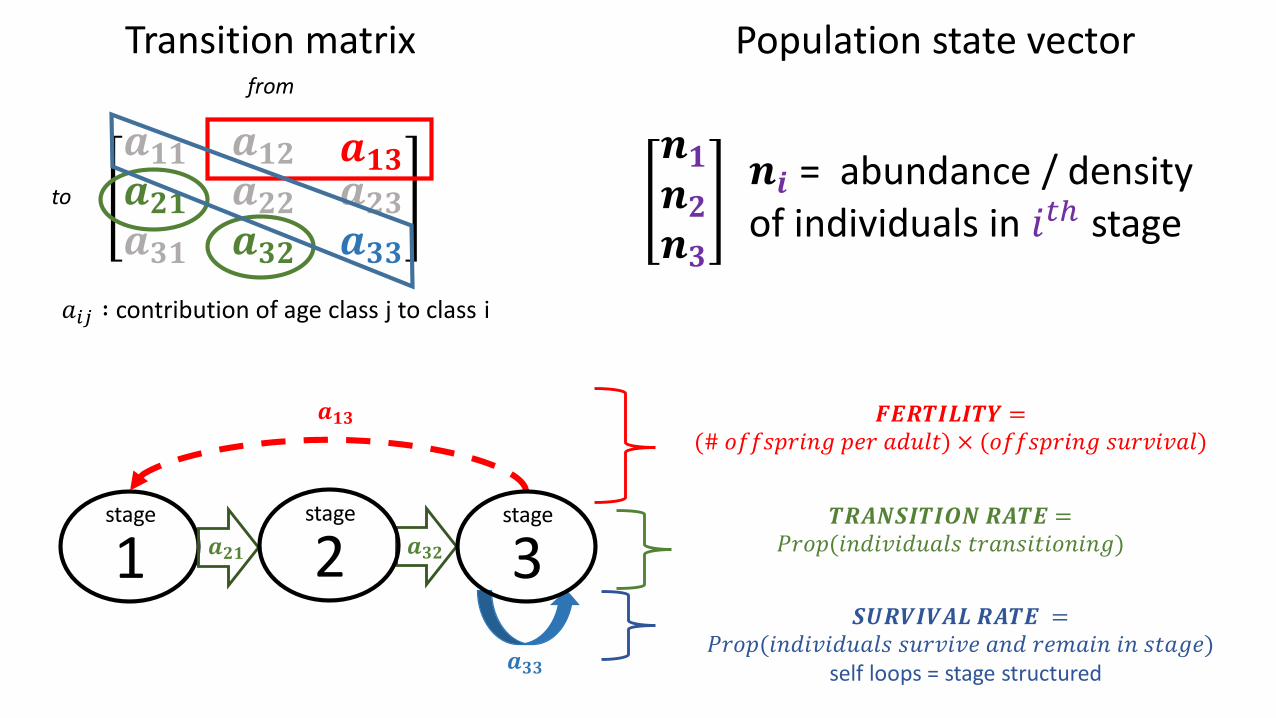
Transition matrix
𝒂𝟏𝟏 𝒂𝟏𝟐 𝒂𝟏𝟑𝒂𝟐𝟏𝒂𝟑𝟏
𝒂𝟐𝟐𝒂𝟑𝟐
𝒂𝟐𝟑𝒂𝟑𝟑
1
𝑎𝑖𝑗 ∶ contribution of age class j to class i
from
to
𝒂𝟑𝟑
𝒂𝟐𝟏 𝒂𝟑𝟐
𝒂𝟏𝟑 𝑭𝑬𝑹𝑻𝑰𝑳𝑰𝑻𝒀 =(# 𝑜𝑓𝑓𝑠𝑝𝑟𝑖𝑛𝑔 𝑝𝑒𝑟 𝑎𝑑𝑢𝑙𝑡) × (𝑜𝑓𝑓𝑠𝑝𝑟𝑖𝑛𝑔 𝑠𝑢𝑟𝑣𝑖𝑣𝑎𝑙)
stage
2stage
3stage 𝑻𝑹𝑨𝑵𝑺𝑰𝑻𝑰𝑶𝑵 𝑹𝑨𝑻𝑬 =
𝑃𝑟𝑜𝑝(𝑖𝑛𝑑𝑖𝑣𝑖𝑑𝑢𝑎𝑙𝑠 𝑡𝑟𝑎𝑛𝑠𝑖𝑡𝑖𝑜𝑛𝑖𝑛𝑔)
𝑺𝑼𝑹𝑽𝑰𝑽𝑨𝑳 𝑹𝑨𝑻𝑬 =𝑃𝑟𝑜𝑝(𝑖𝑛𝑑𝑖𝑣𝑖𝑑𝑢𝑎𝑙𝑠 𝑠𝑢𝑟𝑣𝑖𝑣𝑒 𝑎𝑛𝑑 𝑟𝑒𝑚𝑎𝑖𝑛 𝑖𝑛 𝑠𝑡𝑎𝑔𝑒)
self loops = stage structured
𝒏𝟏𝒏𝟐𝒏𝟑
𝒏𝒊 = abundance / density of individuals in 𝑖𝑡ℎ stage
Population state vector
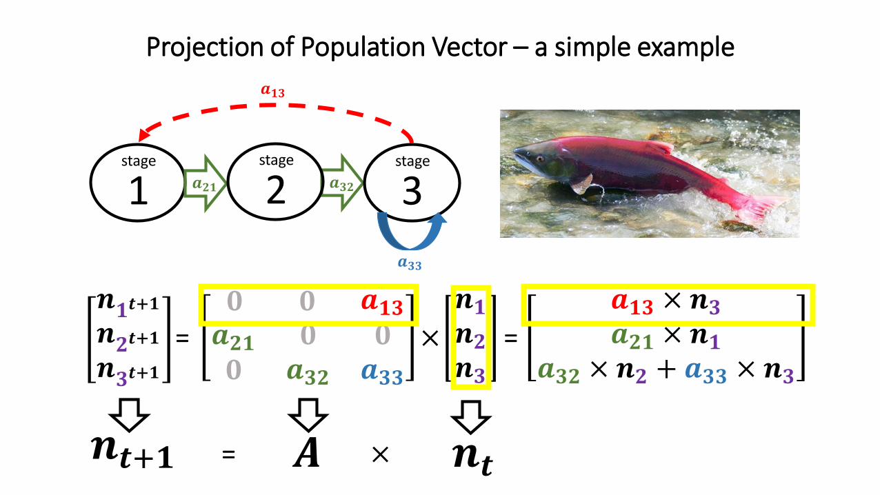
Projection of Population Vector – a simple example
𝒏𝟏𝒕+𝟏𝒏𝟐𝒕+𝟏𝒏𝟑𝒕+𝟏
𝟎 𝟎 𝒂𝟏𝟑𝒂𝟐𝟏𝟎
𝟎𝒂𝟑𝟐
𝟎𝒂𝟑𝟑
𝒏𝟏𝒏𝟐𝒏𝟑
= ×
1 𝒂𝟐𝟏 𝒂𝟑𝟐
𝒂𝟏𝟑
stage
2stage
3stage
=
𝒂𝟏𝟑 × 𝒏𝟑𝒂𝟐𝟏 × 𝒏𝟏
𝒂𝟑𝟐 × 𝒏𝟐 + 𝒂𝟑𝟑 × 𝒏𝟑
𝑨 𝒏𝒕𝒏𝒕+𝟏 = ×
𝒂𝟑𝟑
𝒏𝟏𝒕+𝟏𝒏𝟐𝒕+𝟏𝒏𝟑𝒕+𝟏
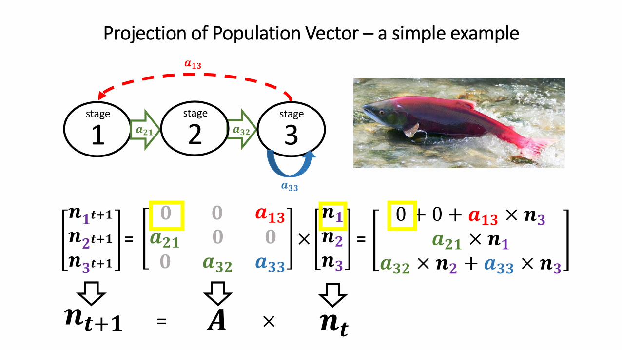
Projection of Population Vector – a simple example
𝟎 𝟎 𝒂𝟏𝟑𝒂𝟐𝟏𝟎
𝟎𝒂𝟑𝟐
𝟎𝒂𝟑𝟑
𝒏𝟏𝒏𝟐𝒏𝟑
= ×
1 𝒂𝟐𝟏 𝒂𝟑𝟐
𝒂𝟏𝟑
stage
2stage
3stage
=0 + 0 + 𝒂𝟏𝟑 × 𝒏𝟑
𝒂𝟐𝟏 × 𝒏𝟏𝒂𝟑𝟐 × 𝒏𝟐 + 𝒂𝟑𝟑 × 𝒏𝟑
𝑨 𝒏𝒕𝒏𝒕+𝟏 = ×
𝒂𝟑𝟑

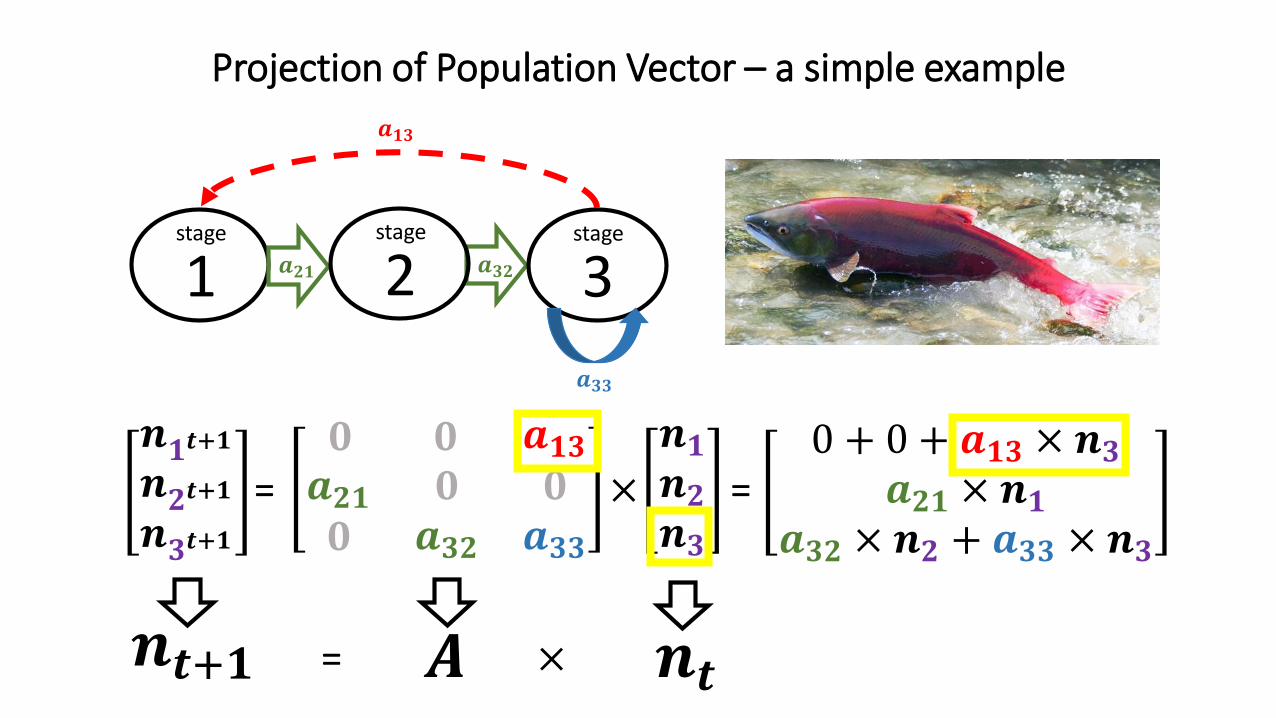
Projection of Population Vector – a simple example
𝒏𝟏𝒕+𝟏𝒏𝟐𝒕+𝟏𝒏𝟑𝒕+𝟏
𝟎 𝟎 𝒂𝟏𝟑𝒂𝟐𝟏𝟎
𝟎𝒂𝟑𝟐
𝟎𝒂𝟑𝟑
𝒏𝟏𝒏𝟐𝒏𝟑
= ×
1 𝒂𝟐𝟏 𝒂𝟑𝟐
𝒂𝟏𝟑
stage
2stage
3stage
=0 + 0 + 𝒂𝟏𝟑 × 𝒏𝟑
𝒂𝟐𝟏 × 𝒏𝟏𝒂𝟑𝟐 × 𝒏𝟐 + 𝒂𝟑𝟑 × 𝒏𝟑
𝑨 𝒏𝒕𝒏𝒕+𝟏 = ×
𝒂𝟑𝟑
𝒏𝟏𝒕+𝟏𝒏𝟐𝒕+𝟏𝒏𝟑𝒕+𝟏
Projection of Population Vector – a simple example
𝟎 𝟎 𝒂𝟏𝟑𝒂𝟐𝟏𝟎
𝟎𝒂𝟑𝟐
𝟎𝒂𝟑𝟑
𝒏𝟏𝒏𝟐𝒏𝟑
= ×
1 𝒂𝟐𝟏 𝒂𝟑𝟐
𝒂𝟏𝟑
stage
2stage
3stage
=0 + 0 + 𝒂𝟏𝟑 × 𝒏𝟑
𝒂𝟐𝟏 × 𝒏𝟏𝒂𝟑𝟐 × 𝒏𝟐 + 𝒂𝟑𝟑 × 𝒏𝟑
𝑨 𝒏𝒕𝒏𝒕+𝟏 = ×
𝒂𝟑𝟑
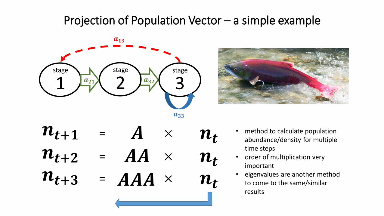
Projection of Population Vector – a simple example
1 𝒂𝟐𝟏 𝒂𝟑𝟐
𝒂𝟏𝟑
stage
2stage
3stage
𝑨 𝒏𝒕𝒏𝒕+𝟏 = ×
𝒂𝟑𝟑
𝑨𝑨 𝒏𝒕𝒏𝒕+𝟐 = ×
𝑨𝑨𝑨 𝒏𝒕𝒏𝒕+𝟑 = ×
• method to calculate population abundance/density for multiple time steps
• order of multiplication very important
• eigenvalues are another method to come to the same/similar results
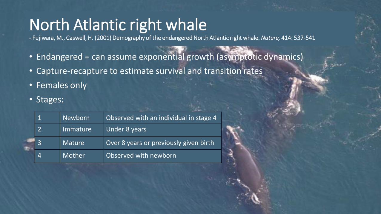
North Atlantic right whale - Fujiwara, M., Caswell, H. (2001) Demography of the endangered North Atlantic right whale. Nature, 414: 537-541
• Endangered = can assume exponential growth (asymptotic dynamics)
• Capture-recapture to estimate survival and transition rates
• Females only
• Stages:
1 Newborn Observed with an individual in stage 4
2 Immature Under 8 years
3 Mature Over 8 years or previously given birth
4 Mother Observed with newborn
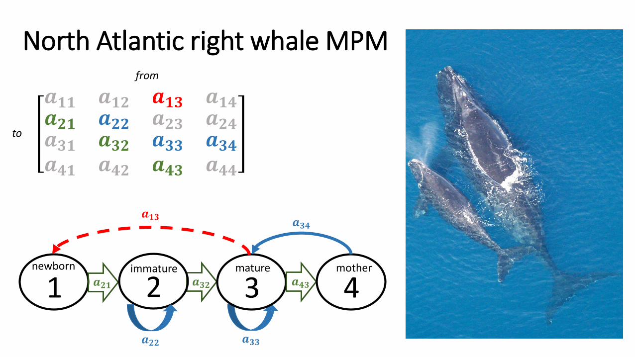
North Atlantic right whale MPM
𝒂𝟏𝟏 𝒂𝟏𝟐 𝒂𝟏𝟑 𝒂𝟏𝟒𝒂𝟐𝟏𝒂𝟑𝟏𝒂𝟒𝟏
𝒂𝟐𝟐𝒂𝟑𝟐𝒂𝟒𝟐
𝒂𝟐𝟑 𝒂𝟐𝟒𝒂𝟑𝟑 𝒂𝟑𝟒𝒂𝟒𝟑 𝒂𝟒𝟒
1
from
to
𝒂𝟑𝟑
𝒂𝟐𝟏 𝒂𝟑𝟐
𝒂𝟑𝟒
newborn
2 3 𝒂𝟒𝟑 4
𝒂𝟐𝟐
𝒂𝟏𝟑
immature mature mother
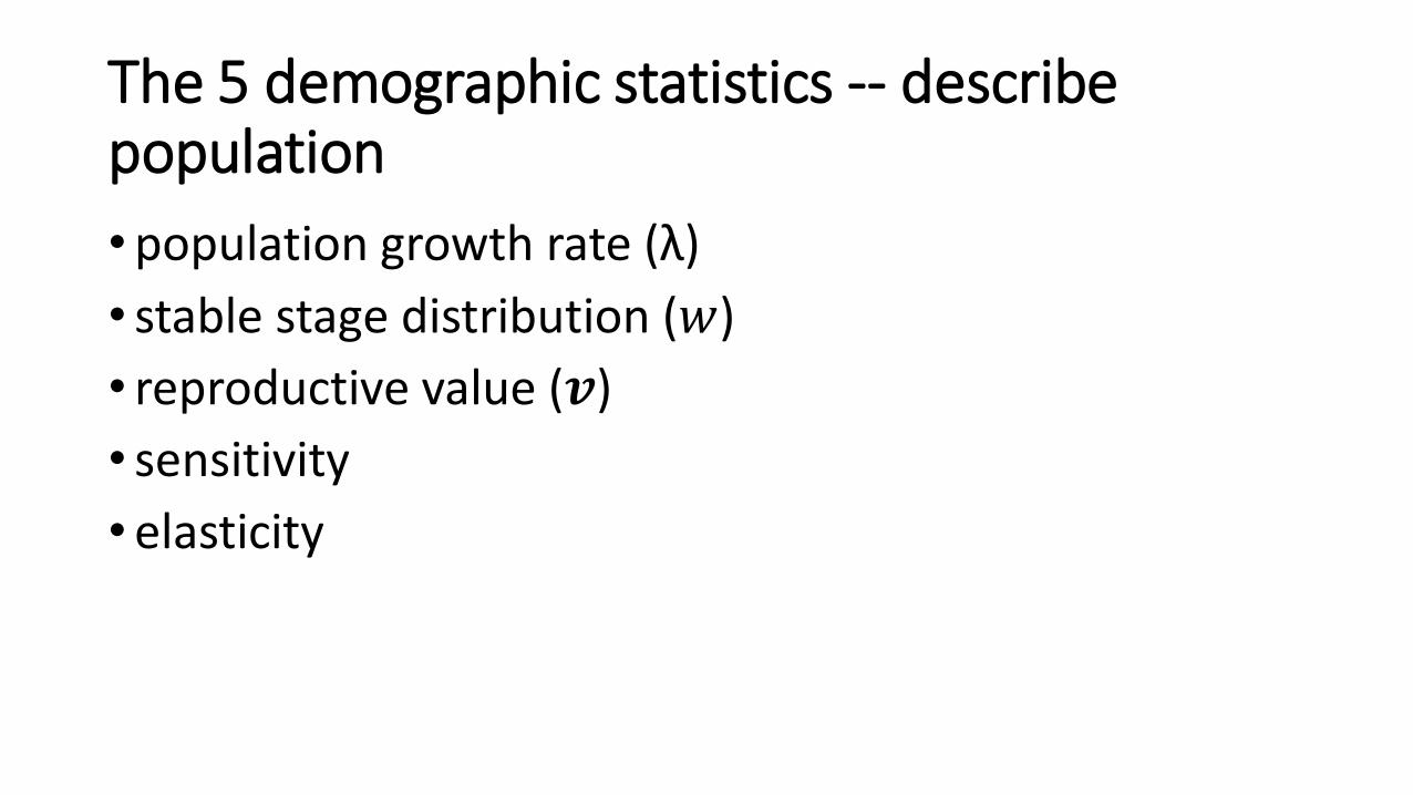
The 5 demographic statistics -- describe population
•population growth rate (λ)
• stable stage distribution (𝑤)
• reproductive value (𝒗)
• sensitivity
• elasticity
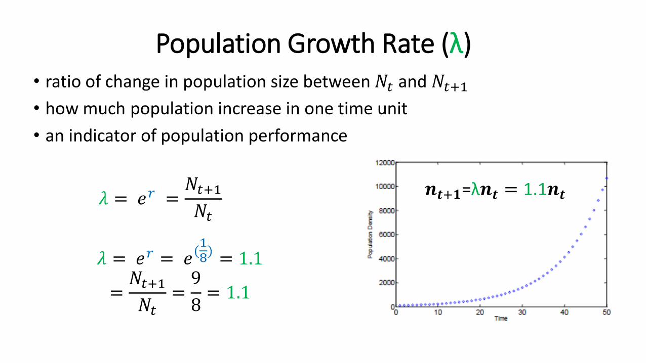
Population Growth Rate (λ)• ratio of change in population size between 𝑁𝑡 and 𝑁𝑡+1• how much population increase in one time unit
• an indicator of population performance
𝜆 = 𝑒𝑟 =𝑁𝑡+1𝑁𝑡
𝜆 = 𝑒𝑟 = 𝑒(18) = 1.1
=𝑁𝑡+1𝑁𝑡
=9
8= 1.1
𝒏𝒕+𝟏=λ𝒏𝒕 = 1.1𝒏𝒕
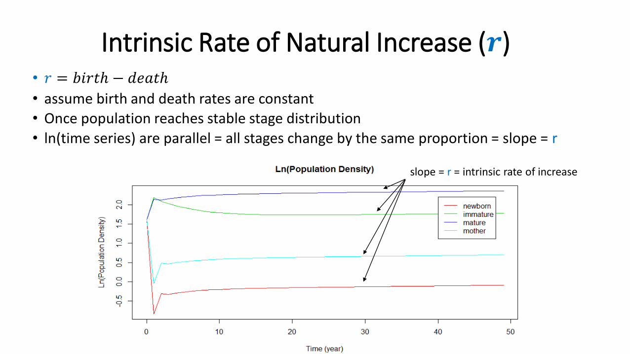
Intrinsic Rate of Natural Increase (𝒓)• 𝑟 = 𝑏𝑖𝑟𝑡ℎ − 𝑑𝑒𝑎𝑡ℎ
• assume birth and death rates are constant • Once population reaches stable stage distribution
• ln(time series) are parallel = all stages change by the same proportion = slope = r
slope = r = intrinsic rate of increase
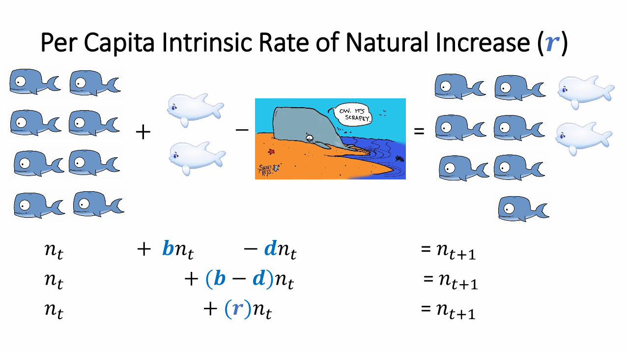
𝑛𝑡 + 𝒃𝑛𝑡 − 𝒅𝑛𝑡 = 𝑛𝑡+1𝑛𝑡 + (𝒃 − 𝒅)𝑛𝑡 = 𝑛𝑡+1𝑛𝑡 + (𝒓)𝑛𝑡 = 𝑛𝑡+1
+ − =
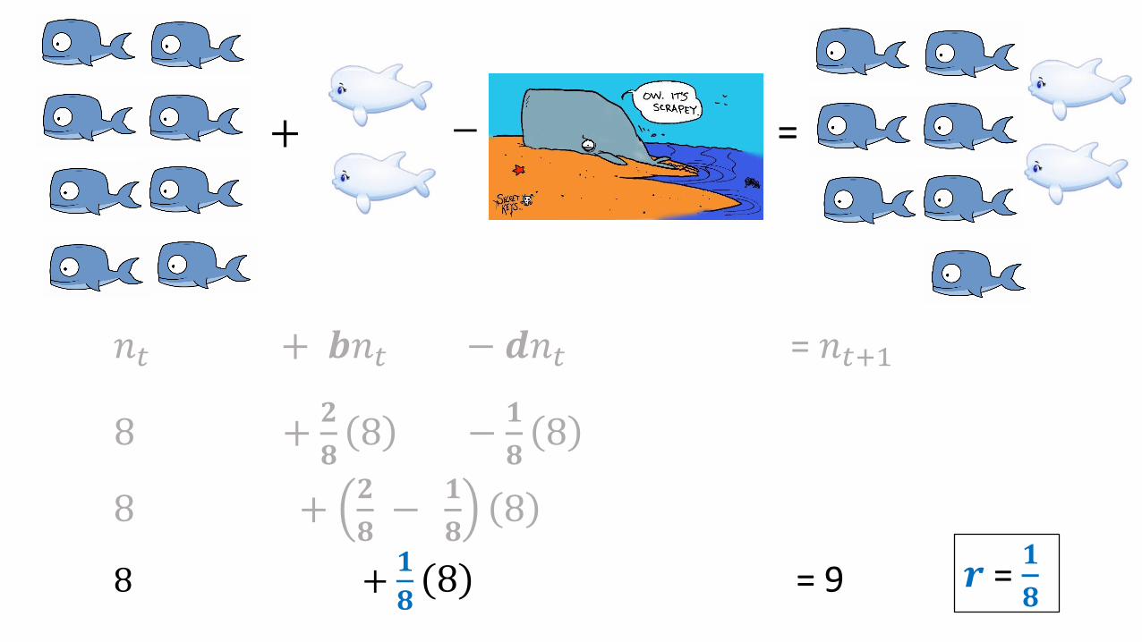
Per Capita Intrinsic Rate of Natural Increase (𝒓)

𝑛𝑡 + 𝒃𝑛𝑡 − 𝒅𝑛𝑡 = 𝑛𝑡+1
8 +𝟐
𝟖8 −
𝟏
𝟖8
+ − =
*per capita rates

𝑛𝑡 + 𝒃𝑛𝑡 − 𝒅𝑛𝑡 = 𝑛𝑡+1
8 +𝟐
𝟖8 −
𝟏
𝟖8
8 +𝟐
𝟖−
𝟏
𝟖8
+ − =
𝑛𝑡 + 𝒃𝑛𝑡 − 𝒅𝑛𝑡 = 𝑛𝑡+1
8 +𝟐
𝟖8 −
𝟏
𝟖8
8 +𝟐
𝟖−
𝟏
𝟖8
+ − =
8 +𝟏
𝟖8 = 9 𝒓 =
𝟏
𝟖
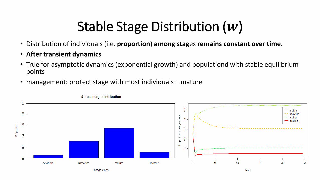
Stable Stage Distribution (𝒘)• Distribution of individuals (i.e. proportion) among stages remains constant over time.
• After transient dynamics
• True for asymptotic dynamics (exponential growth) and populationd with stable equilibrium points
• management: protect stage with most individuals – mature
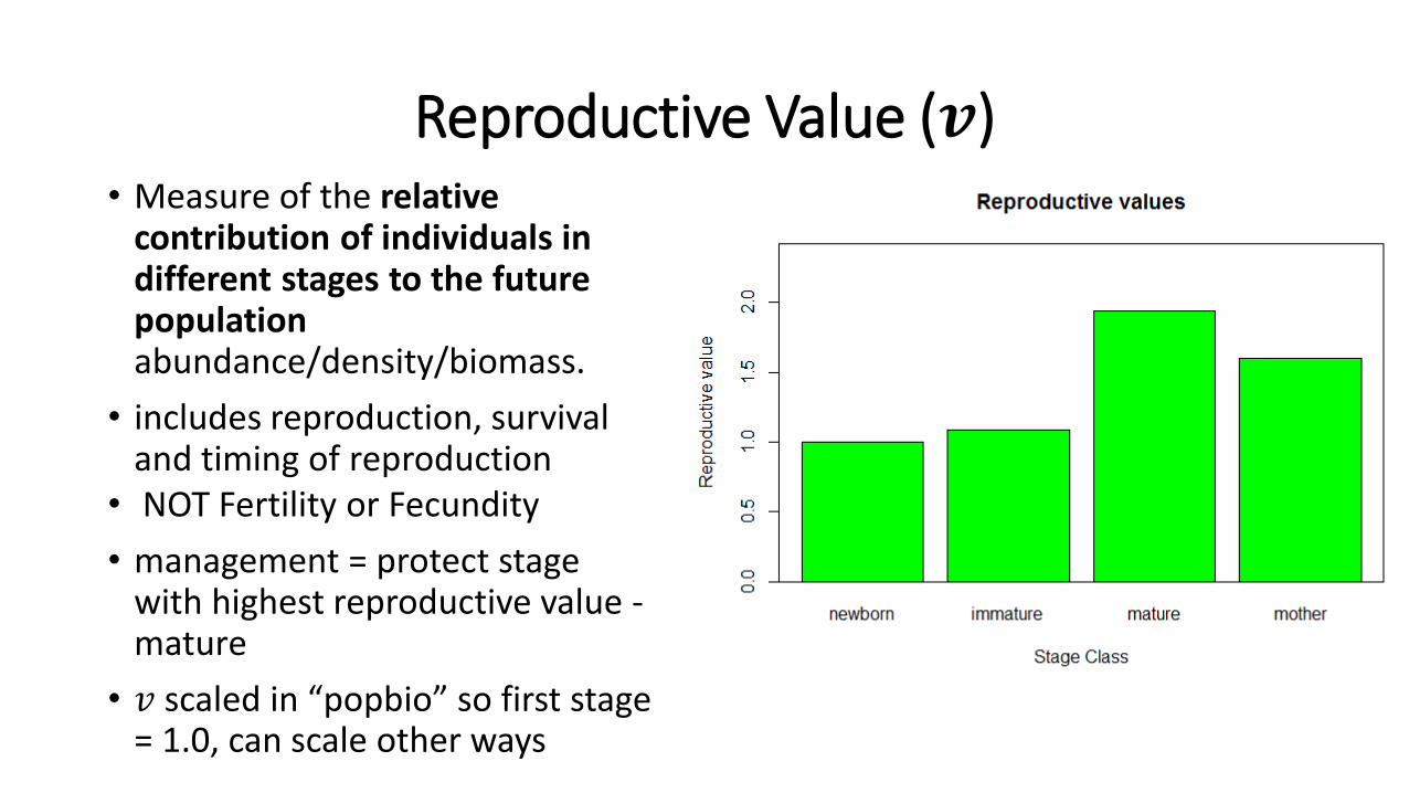
Reproductive Value (𝒗) • Measure of the relative
contribution of individuals in different stages to the future population abundance/density/biomass.
• includes reproduction, survival and timing of reproduction
• NOT Fertility or Fecundity
• management = protect stage with highest reproductive value -mature
• 𝑣 scaled in “popbio” so first stage = 1.0, can scale other ways
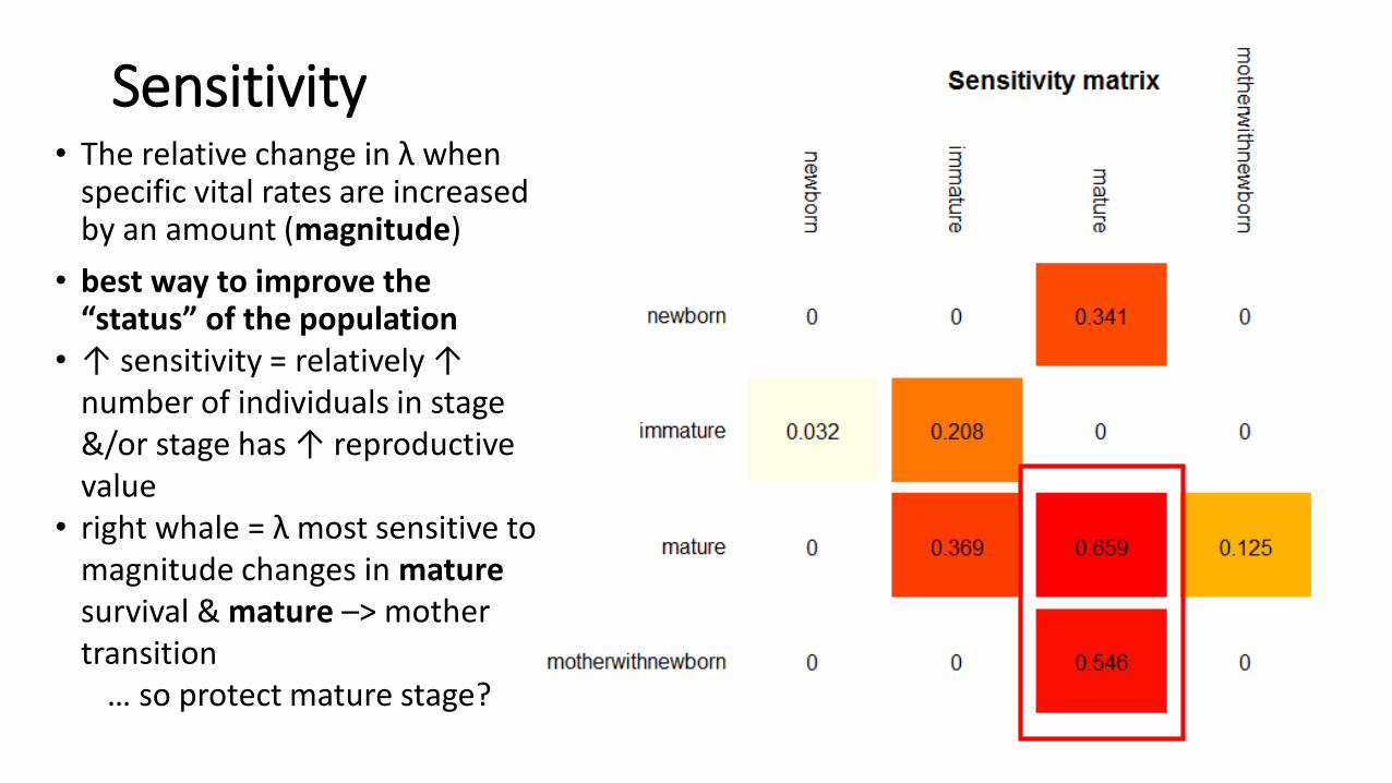
Sensitivity• The relative change in λ when
specific vital rates are increased by an amount (magnitude)
• best way to improve the “status” of the population
• ↑ sensitivity = relatively ↑ number of individuals in stage &/or stage has ↑ reproductive value
• right whale = λ most sensitive to magnitude changes in maturesurvival & mature –> mother transition
… so protect mature stage?

must always consider feasibility …
0 00.92 0.86
0.0865 00 0
0 0.080 0
0.80 0.830.19 0
• Mature survival = 0.99 already • so… best management option
according to sensitivity analysis = increase transition from immature to mature
Transition Matrix
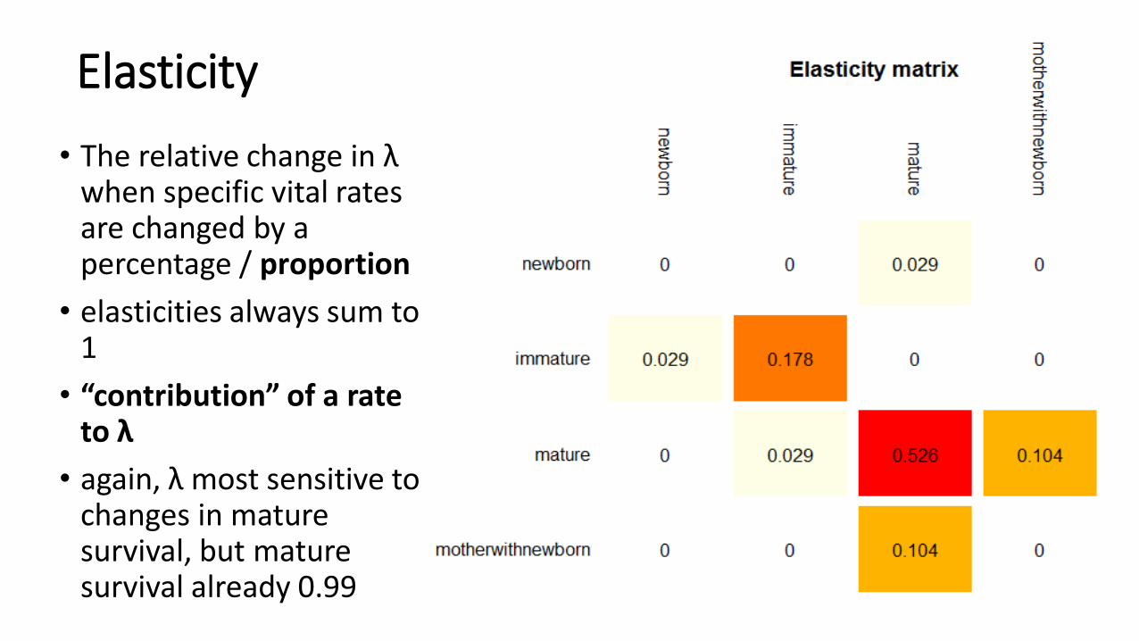
Elasticity
• The relative change in λwhen specific vital rates are changed by a percentage / proportion
• elasticities always sum to 1
• “contribution” of a rate to λ
• again, λ most sensitive to changes in mature survival, but mature survival already 0.99
RESOURCES
• Caswell, H. (2001). Matrix population models. John Wiley & Sons, Ltd.
• Caswell, H., & Fujiwara, M. (2004). Beyond survival estimation: mark-recapture, matrix population models, and population dynamics. Animal Biodiversity and Conservation, 27(1), 471-488.
• Fujiwara, M., & Caswell, H. (2001). Demography of the endangered North Atlantic right whale. Nature, 414(6863), 537-541.
• Stubben, C., & Milligan, B. (2007). Estimating and analyzing demographic models using the popbio package in R. Journal of Statistical Software, 22(11), 1-23.
Related Documents