THEORY Linear isotropic poroelasticity. The constitutive equations are adopted from 1 and are an extension of linear elasticity to poroelastic materials first introduced by Biot 2 . Alternatively one can use the biphasic model 3 that has been extensively applied in modelling the mechanics of cartilage and other soft hydrated tissues. The Biot formulation can be simplified when poroelastic parameters assume their limiting values. Under the “incompressible constituents” condition, the material exhibits its strongest poroelastic effect and the Biot poroelastic theory can be mathematically transformed to the biphasic model. We consider the quasi-static process of isotropic fully saturated poroelastic medium with constant porosity. The constitutive equation relates the total stress tensor σ to the infinitesimal strain tensor ε of the solid phase and the pore fluid pressure p : - 2 2 {tr } , (1 2 ) s s s s G G p n n σ ε ε I I (1) where s G and s n are the shear modulus and the Poisson ratio of the drained network respectively, I the identity tensor, tr the trace operator and tr q ε the variation in fluid content. This equation is similar to the constitutive governing equation for conventional single phase linear elastic materials. However the time dependent properties are incorporated through the pressure term acting as an additional external force on the solid phase. In the absence of body forces and neglecting the inertial terms the equilibrium equation div 0 σ results in: 2 div 0, (1 2 ) s s s G G p n u u+ (2) where u is the vector of solid displacement for small deformations 0.5 T u u ε , div , and 2 designate the divergence, gradient and Laplacian operators, respectively. Next, we consider fluid transport inside the porous medium through the introduction of Darcy’s law: K p q , where q is the filtration velocity and K the hydraulic permeability. Combining the continuity equation div / t q q and Darcy’s law yields: 2 . K p t q (3) We obtain the diffusion equation for q by combining equations (2) and (3) into what is called the consolidation equation: 2 , P D t q q (4) where p D is the poroelastic diffusion coefficient: 2 (1 ) (1 2 ) s s p s G D K n n (5) Derivation of the diffusion equation implies that under the assumptions made here, there are three independent parameters that characterize the mechanical properties of poroelastic cytoplasm: s G , p D , and s n . The cytoplasm of living cells behaves as a poroelastic material SUPPLEMENTARY INFORMATION DOI: 10.1038/NMAT3517 NATURE MATERIALS | www.nature.com/naturematerials 1 © 2013 Macmillan Publishers Limited. All rights reserved.

Welcome message from author
This document is posted to help you gain knowledge. Please leave a comment to let me know what you think about it! Share it to your friends and learn new things together.
Transcript
1
SUPPLEMENTARY INFORMATION
THEORY Linear isotropic poroelasticity. The constitutive equations are adopted from1 and are an extension of linear elasticity to poroelastic materials first introduced by Biot 2. Alternatively one can use the biphasic model 3 that has been extensively applied in modelling the mechanics of cartilage and other soft hydrated tissues. The Biot formulation can be simplified when poroelastic parameters assume their limiting values. Under the “incompressible constituents” condition, the material exhibits its strongest poroelastic effect and the Biot poroelastic theory can be mathematically transformed to the biphasic model. We consider the quasi-static process of isotropic fully saturated poroelastic medium with constant porosity. The constitutive equation relates the total stress tensor σ to the infinitesimal strain tensor ε of the solid phase and the pore fluid pressure p :
-2
2 {tr } ,(1 2 )
s ss
s
GG p
nn
σ ε ε I I (1)
where sG and sn are the shear modulus and the Poisson ratio of the drained network respectively, I the identity tensor, tr the trace operator and tr q ε the variation in fluid content. This equation is similar to the constitutive governing equation for conventional single phase linear elastic materials. However the time dependent properties are incorporated through the pressure term acting as an additional external force on the solid phase. In the absence of body forces and neglecting the inertial terms the equilibrium equation div 0σ results in:
2 div 0,(1 2 )
ss
s
GG pn
uu + (2)
where u is the vector of solid displacement for small deformations 0.5 Tu uε , div , and 2 designate the divergence, gradient and Laplacian operators, respectively. Next, we consider fluid transport inside the porous medium through the introduction of Darcy’s law: K pq , where q is the filtration velocity and K the hydraulic permeability. Combining the continuity equation div / tqq and Darcy’s law yields:
2 .K ptq
(3)
We obtain the diffusion equation for q by combining equations (2) and (3) into what is called the consolidation equation:
2 ,PDtq
q (4)
where pD is the poroelastic diffusion coefficient:
2 (1 )(1 2 )s s
ps
GD Knn
(5)
Derivation of the diffusion equation implies that under the assumptions made here, there are three independent parameters that characterize the mechanical properties of poroelastic cytoplasm: sG , pD , and sn .
The cytoplasm of living cells behaves as a poroelastic material
SUPPLEMENTARY INFORMATIONDOI: 10.1038/NMAT3517
NATURE MATERIALS | www.nature.com/naturematerials 1
© 2013 Macmillan Publishers Limited. All rights reserved.
2
Scaling of diffusion coefficient with microstructural parameters. The most important consequence of
considering a poroelastic cytoplasm is that the macroscopic mechanical properties of the cell can be related to
some coarse-grained cellular microstructural parameters. As a first step, to understand the relationship between
microstructure and hydraulic permeability, we assume that pores within the solid matrix have an average radius of
x . A simple analogy between a Poiseuille flow inside a tube with radius x and flow through the porous media
with porosity j leads to the following relationship for the hydraulic permeability K
2
,4
Kj xk m
(6)
where m is the viscosity of the fluid and k is a constant taking into account the irregularity, interconnectivity and
tortuosity of the pores 4. Substituting this equivalent expression for the hydraulic permeability into equation (5)
results in:
2(1 ).
(1 )(1 2 ) 4s
ps s
ED
n j xn n k m
(7)
As a first approximation, all of the parameters inside the parenthesis can be assumed to be a constant a and the
functional dependence of all parameters with respect to the porosity of the structure is neglected. Therefore, a
fundamental scaling law for poroelastic cytoplasm takes the form:
2
,p
ED
xa
m (8)
where m is interpreted as the interstitial fluid viscosity, and 2 1s sE G n the elasticity of the constituent
solid network.
© 2013 Macmillan Publishers Limited. All rights reserved.
3
METHODS
Cell culture. HeLa cells, HT1080, and MDCK cells were cultured at 37°C in an atmosphere of 5% CO2 in air in
DMEM (Gibco Life Technologies, Paisley, UK) supplemented with 10% FCS (Gibco Life Technologies) and 1%
Penicillin/Streptomycin. Cells were cultured onto 50 mm glass bottomed Petri dishes (Fluorodish, World
Precision Instruments, Milton Keynes, UK). Prior to the experiment, the medium was replaced with Leibovitz L-
15 without phenol red (Gibco Life Technologies) supplemented with 10% FCS.
Generation of cell lines, transduction, and molecular biology. To enable imaging of the cell membrane, we
created a stable cell line expressing the PH domain of Phospholipase Cδ tagged with GFP (PHPLCδ-GFP), a
phosphatidyl-inositol-4,5-bisphophate binding protein that localises to the cell membrane. Briefly, PH-PLCδ-GFP
(a kind gift from Dr Tamas Balla, NIH) was excised from EGFP-N1 (Takara-Clontech Europe, St Germain en
Laye, France), inserted into the retroviral vector pLNCX2 (Takara-Clontech), and transfected into 293-GPG cells
for packaging (a kind gift from Prof Daniel Ory, Washington University 5). Retroviral supernatants were then used
to infect wild type HeLa cells, cells were selected in the presence of 1 mg.ml-1
G418 (Merck Biosciences UK,
Nottingham, UK) for 2 weeks and subcloned to obtain a monoclonal cell line. Using similar methods, we created
cell lines stably expressing cytoplasmic GFP for cell volume estimation, GFP-actin or Life-act Ruby (6, a kind gift
of Dr Roland Wedlich-Soldner, MPI-Martinsried, Germany) for examination of the F-actin cytoskeleton, GFP-
tubulin for examination of the microtubule cytoskeleton, and GFP-Keratin 18 (a kind gift of Dr Rudolf Leube,
University of Aachen, Germany) for visualisation of the intermediate filament network. HT1080 cells expressing
mCherry-LifeAct and MDCK cells expressing PHPLCδ-GFP were generated using similar methods. The EGFP-
10x plasmid was described in 7 and obtained through Euroscarf (Frankfurt, Germany). Cells were transfected with
cDNA using lipofectamine 2000 according to manufacturer instructions the night before measurements.
Pharmacological treatments for disrupting the cytoskeleton. Cells were incubated in culture medium with the
relevant concentration of drug for 30 min prior to measurement. The medium was then replaced with L-15 with
10% FCS plus the same drug concentration such that the inhibitor was present at all times during measurements.
Cells were treated with latrunculin B (to depolymerise F-actin, Merck-Biosciences), nocodazole (to depolymerise
microtubules, Merck-Biosciences), paclitaxel (to stabilize microtubules, Merck-Biosciences), and blebbistatin (to
inhibit myosin II ATPase, Merck-Biosciences).
Genetic treatments for perturbing the cytoskeleton. To examine the effect of uncontrolled polymerization of
cytoplasmic F-actin, we transduced HeLa cells stably expressing Life-act ruby with lentivirus encoding WASp
I294T as described in 8. Lentiviral vectors expressing enhanced GFP fused to human WASp with the I294T
mutation were prepared in the pHR’SIN-cPPT-CE and pHR’SIN-cPPT-SE lentiviral backbones as described
previously 8,9
. Lentivirus was added to cells at a multiplicity of infection of 10 to achieve approximately 90%
transduction.
To examine the effect of uncontrolled polymerisation of tubulin, we transfected HeLa cells with a plasmid
encoding γ-tubulin, a microtubule nucleator 10
. pγ-tubulin-SNAP 11
was obtained from Euroscarf, the SNAP tag
was excised and replaced by mCherry. To disrupt the keratin nework of HeLa cells, we overexpressed keratin 14
R125C-YFP (a kind gift from Prof Thomas Magin, University of Leipzig), a construct that acts as a dominant
mutant and results in aggregation of endogenous keratins12
. To disrupt F-actin crosslinking by endogenous α-
actinin, we transfected cells with a deletion mutant of α-actinin lacking an actin-binding domain (ΔABD-α-
actinin, a kind gift of Dr Murata-Hori, Temasek Life Sciences laboratory, Singapore). Cells were transfected with
cDNA using lipofectamine 2000 the night before experimentation.
Visualising cytoplasmic F-actin. To visualise cytoplasmic F-actin density, cells were fixed for 15 minutes with
4% PFA at room temperature, permeabilised with 0.1% Triton-X on ice for 5 min, and passivated by incubation
with phosphate buffered saline (PBS) and 10 mg/ml bovine serum albumin (BSA) for 10 min. They were then
stained with Rhodamine-Phalloidin (Invitrogen) for 30 min at room temperature, washed several times with PBS-
BSA, and mounted for microscopy examination on a confocal microscope.
Imaging of cell volume changes. To measure changes in cell volume in response to osmotic shock, confocal
stacks of cells expressing cytoplasmic GFP were acquired at 2 min intervals using a spinning disk confocal
microscope (Yokogawa CSU-22, Yokogawa, Japan) with 100x oil immersion objective lens (NA=1.3, Olympus,
Berlin, Germany) and a piezo-electric z-drive (NanoscanZ, Prior, Scientific, Rockland, MA). Stacks consisted of
© 2013 Macmillan Publishers Limited. All rights reserved.
4
40 images separated by 0.2 µm and were acquired for a total of 30 min and captured on an Andor iXon EMCDD
camera.
Changes in osmolarity
Changes in extracellular osmolarity were effected by adding a small volume of concentrated sucrose, 400-Dalton
polyethylene glycol (PEG-400, Sigma-Aldrich, 13
), or water to the imaging medium. When increasing osmolarity
by addition of osmolyte, we treated MDCK cells with EIPA (50 µM, Sigma-Aldrich), an inhibitor of regulatory
volume increases 14
. When decreasing the osmolarity by addition of water, we treated the cells simultaneously
with inhibitors of regulatory volume decreases, NPPB (200 μM; Tocris, Bristol, UK) and DCPIB (50 µM, Tocris),
to achieve a sustained volume increase. Cells were incubated with these inhibitors for 30 minutes prior to the
addition of water.
Fluorescence and confocal imaging. In some experiments, we acquired fluorescence images of the cells using an
IX-71 microscope interfaced to the AFM head and equipped with an EMCCD camera (Orca-ER, Hamamatsu,
Germany) piloted using µManager (Micromanager, Palo-Alto, CA). Fluorophores were excited with
epifluorescence and the appropriate filter sets and images were acquired with a 40x dry objective (NA=0.7). For
staining of the nucleus, cells were incubated with Hoechst 34332 (1 µg/ml for 5 min, Merck-Biosciences).
In some cases, to image the cellular indentation in zx-plane, we utilized an AFM interfaced to a confocal laser
scanning microscope (FV1000, Olympus). Images were acquired with a 100x oil immersion objective lens
(NA=1.3, Olympus). Latex beads attached to AFM cantilevers were imaged by exciting with a 647 nm laser and
collecting light at 680 nm. GFP tagged proteins were excited with a 488 nm laser and light was collected at 525
nm. Ruby or Cherry tagged proteins were excited with a 568 nm laser and light was collected at 620 nm. zx-
confocal images passing through the centre of the bead were acquired with 0.2 µm steps in z to give a side view of
the cell before and during indentation or before and after change in extracellular osmolarity (Fig. 1C, Fig. S1F).
Calculating cell volume. Exposure time and laser intensity were optimised to minimize photobleaching. A
custom written code in Matlab (Mathworks Inc, Cambridge, UK) was used to process the z stacks and measure
the cell volume at each time point. Briefly, the background noise of stack images was removed, images were
smoothed, and binarised using Matlab Image Processing Toolbox functions. Following binarization, series of
erosion and dilatation operations were performed to create a contiguous cell volume image devoid of isolated
pixels. The sum of non-zero pixels in each stack was multiplied by the volume of a voxel to give a measure of cell
volume at each time step. All experiments followed the same protocol: five stacks were captured prior to changing
osmolarity and then cell volume was followed for a further 25 minutes.
Atomic force Microscopy measurements. Force-distance and force-relaxation measurements were acquired with
a JPK Nanowizard-I (JPK instruments, Berlin, Germany) interfaced to an inverted optical fluorescence
microscope (IX-81 or IX-71, Olympus).
AFM cantilevers (MLCT, Bruker, Karlsruhe, Germany) were modified by gluing beads to the cantilever underside
with UV curing glue (UV curing, Loctite, UK). Cantilever spring constants were determined prior to gluing the
beads using the thermal noise method implemented in the AFM software (JPK SPM, JPK instruments). Prior to
any cellular indentation tests, the sensitivity of the cantilever was set by measuring the slope of force-distance
curves acquired on glass regions of the petri dish. For measurements on cells, we used cantilevers with nominal
spring constants of 0.01 N.m-1
and fluorescent latex beads (ex645/em680, R=7.5 μm, Invitrogen). For
measurements on hydrogels, we used cantilevers with nominal spring constants of 0.6 N.m-1
and glass beads
(R=25 μm, Sigma).
During force-relaxation measurements, we used the z-closed loop feedback implemented on the JPK Nanowizard
to maintain a constant z-piezo height. When acquiring force-relaxation curves with high approach velocities
(Vapproach>10 μms-1
), the first 5 ms of force-relaxation were not considered in the data analysis due to the presence
of small oscillations in z-piezoelectric ceramic height immediately after contact. When acquiring force-relaxations
curves for averaging over multiple cells, we used approach velocities Vapproach~10 μm.s-1
that did not give rise to
oscillations in the length of the z-piezoelectric ceramic.
Hydrogels. For comparison with cells, we acquired force-relaxations measurements on physical hydrogels, which
are well-characterised poroelastic materials. For measurements, we made gels with a 15% solution of a 20:1 mix
of acrylamide-bis-acrylamide crosslinked with TEMED and ammonium persulfate following the manufacturer’s
instructions (Bio-Rad, UK).
© 2013 Macmillan Publishers Limited. All rights reserved.
5
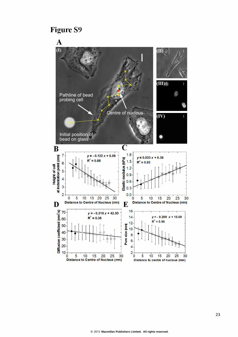
Cell height and spatial measurements with AFM. To investigate spatial variations in the cellular poroelastic
properties, we acquired measurements at several locations on the cell surface along the long axis of the cell with a
target force of FM =4 nN. To locate indentation points on optical images of the cell, a fluorescence image of the
bead resting on the glass surface close to the cell was acquired and the bead centre used as a reference point (see
Fig. S9A). This reference point was used to estimate the height of the cell in each measurement point, as well as
the position of indentation on the cell surface knowing the xy-coordinates of each stress relaxation measurement
from the AFM software. The position of the measurement point relative to the nucleus was estimated by acquiring
a fluorescence image of the nucleus and calculating its centre of mass (see Fig. S9A).
To measure cell height, we collected a force-distance curve on the glass substrate next to the cell being examined
and the height of contact between the probe and the glass was used as a height reference (see Fig. S9A). At each
indentation point, the cell height was estimated by comparing the height of contact to the reference. The position
of contact in force-distance curves was determined using the algorithm described in 15,16
.
Measurement of indentation depth, cellular elastic modulus. The approach phase of AFM force-distance
curves (inset, Fig. 1B-I) was analysed to extract the elastic modulus E which is linearly related to the shear
modulus G through the Poisson ratio E=2G(1+ν). For estimation of the elastic modulus, we assumed a Poisson
ratio ν =0.3. The contact point between the cell and the AFM tip was found using the method described in 15,16
.
The indentation depth δ was calculated by subtracting the cantilever deflection d from the piezo translation z after
contact δ=z-d. E was estimated by fitting the contact portion of the curve with a Hertzian contact model between a
sphere and an infinite half space 17
. The relationship between the applied force F and the indentation depth is:
1/2 3/28
,3 1G
F R dn
(9)
with ν the Poisson ratio, and R the radius of the spherical indenter. To minimise errors arising from finite cell
thickness, we excluded data points where the indentation depth δ was more than a quarter of the cell height h 18-20
.
In our experiments, the cantilever was approached at very high velocity and hence at short times the cytoplasmic
interstitial fluid does not have time to drain out of the compressed region. This represents the undrained condition
for the poroelastic material 1,21
and equation (9) becomes 1/2 3/216
(0)3
F GR d . At long time-scales, the
interstitial fluid redistributes in the cell and the force imposed by the indenter is balanced by stress in the elastic
porous matrix only. Under this condition, the force applied for the prescribed indentation is
1/2 3/28
( )3(1 )s
F GR dn
. Comparing the long time-scale and short time-scale limits allows for estimation of
the Poisson ratio of the solid matrix (0)/ ( ) 2(1 )sF F n . Experimental force-distance curves were analysed
using custom written software in Matlab following the algorithm described in 15
.
Establishing the experimental conditions to measure cellular poroelastic diffusion constant. In our
experiments, after rapid local force application by AFM (6nN applied during a rise time tr of 35ms on HeLa cells,
Fig. 1A-B), the indentation depth increased by an average of ~5% over a 2.5s relaxation period (N=189
measurements, Fig. 1B-I, black), whereas force relaxed by ~35% (Fig. 1B-I, grey). Therefore, we assumed that
the indentation depth and contact area remained constant and our experimental conditions are those of a force-
relaxation problem. In poroelasticity, relaxation following application of force is due to water movement out of
the porous matrix in the displaced region. Hence to truly probe the poroelastic properties of cells, we need to
establish a regime where deformation is applied faster than water can leave the displaced volume. In an
axisymmetric problem, this can be expressed simply by comparing the rise time tr needed to reach an indentation
depth δ to the time needed for water to diffuse out of the displaced volume tp~L2/Dp with L the length-scale of the
problem 22,23
: L~(Rδ)0.5
with R the radius of the indenter. In our experiments, we used an indenter with radius
R=7.5 µm, a typical indentation depth δ=1 µm, and previous experiments suggested Dp~1 to 100 µm2.s
-1
24,25 in
cells yielding characteristic poroelastic times of tp~ 0.1 to 10 s. Hence, given an experimental rise time of tr~35ms,
tr/tp is small compared to 1 signifying that pressurisation of interstitial water occurs and therefore water movement
through the solid matrix contributes strongly to relaxation.
Determining the apparent cellular viscosity. For comparison with previous reports and use in numerical models
of cell dynamics, we determined the apparent cellular viscosity of cells in our experiments using a standard linear
© 2013 Macmillan Publishers Limited. All rights reserved.
6
model consisting of a spring-damper (stiffness k1 and apparent viscosity η) in parallel with another spring
(stiffness k2), as described in 26
. In this model, the applied force decays exponentially when the material is
subjected to a step displacement at t=0:
1( ).
k tf
i f
F t Fe
F Fh (10)
The spring constant k1 scales with the elastic modulus k1~E and therefore we fitted our experimental force-
relaxation curves using equation (10), with η as sole fitting parameter.
Microinjection and imaging of quantum dots. PEG-passivated quantum dots (qdots 705, Invitrogen) were
diluted in injection buffer (50 mM potassium glutamate, 0.5 mM MgCl2, pH 7.0) to achieve a final concentration
of 0.2 μM and microinjected into HeLa cells as described in 27
. Quantum dots were imaged on a spinning disk
confocal microscope by exciting at 488nm and collecting emission above 680 nm. To qualitatively visualize the
extent of quantum dot movement, time series were projected onto one plane using ImageJ.
FRAP experiments. FRAP experiments were performed using a 100x oil immersion objective lens (NA=1.3,
Olympus) on a scanning laser confocal microscope (Olympus Fluoview FV1000; Olympus). Cytoplasmic
fluorophores including GFP-tagged proteins and CMFDA (5-chloromethylfluorescein diacetate, Celltracker
Green, Invitrogen) were excited at 488 nm wavelength. For experiments with CMFDA, cells were incubated with
2 µM CMFDA for 45 min before replacing the medium with imaging medium. For experiments with GFP or
EGFP-10x, cells were transfected with the plasmid of interest the day before experimentation. To obtain a strong
fluorescence signal and minimize photobleaching, a circular region of interest (ROI, 1.4 µm in diameter) in the
middle of the cytoplasm was imaged setting laser power (488nm wave length, nominal output of 20mW) to 5%
and 1% of maximum output for GFP and CMFDA, respectively. Each FRAP experiment started with five image
scans, followed by a 1s bleach pulse produced by scanning the 488nm laser beam line by line (at 100% power for
GFP and 25% power for CMFDA) over a circular bleach region of nominal radius nr =0.5 μm centered in the
middle of the imaging ROI. To sample the recovery with sufficient time resolution, an imaging ROI of radius of
0.7 μm was chosen allowing acquisition with a rate of 50ms per frame.
Effective bleach radius. Because of rapid diffusion of fluorophores within the cytoplasm during the bleaching
process, the effective radius over which photobleaching takes place ( er ) is larger than the nominal radius ( nr ). We
followed the methods described in 28
to fit our FRAP experiments and hence needed to determine re. To
experimentally estimate the effective radius er , we performed a separate series of FRAP experiments on cells
loaded with CMFDA in hyperosmotic conditions. We empirically chose an imaging area larger than the effective
photobleaching radius (4 µm in diameter) and imaged photobleaching recovery at a frame rate of 0.2s/frame.
Next, using a custom written Matlab program, we calculated the radial projection profile of the fluorescence
intensity in the imaging region for the first post-bleach image I(r,t=1) and then fitted the experimental intensity
profile with the bleach equation for a Gaussian laser beam to determine re 28
(Fig. S8A):
2
2( ) exp exp 2 ,
e
rI r K
r (11)
where r is the radial distance from the centre of bleach spot and K is the bleaching constant related to the intensity
of the bleaching laser and the properties of the fluorophore.
FRAP analysis. FRAP recovery curves I(t) were obtained by normalising the mean fluorescence intensity within
the nominal bleach area for each frame to the average fluorescence intensity of the first pre-bleach image. The
translational diffusion coefficient TD was estimated using the model for a uniform-disk laser profile and ideal
bleach 29,30
following the methods described in 28
:
2 2 2
0 1( ) exp ,8 8 8e e e
nT T T
r r rI t I I
D t D t D t (12)
© 2013 Macmillan Publishers Limited. All rights reserved.
7
where In(t)=I(t)/I(∞) is the normalized fluorescence intensity in the bleached spot as a function of time t, re is the
effective bleach radius, I0 and I1 are modified Bessel functions. In the experimentally acquired FRAP curves, the
first post-bleach value In(t=1s) was larger than zero (Fig. 3B,C), something that could be due to rapid fluorophore
diffusion during the bleach process or incomplete bleaching 28
. In cells exposed to hyperosmotic conditions, the
intensity of the first post-bleach time point was over 30% lower than in isoosmotic conditions, suggesting that the
non-zero value of this first time point was due to rapid diffusive recovery. Based on this observation, we assigned
a timing of t=0.1s to the first post-bleach time point when fitting fluorescence recovery curves. The validity of the
fitting was verified by measuring the translational diffusion constant of GFP and CMFDA and comparing these to
previously published values.
Data processing, curve fitting and statistical analysis. Indentation and force-relaxation curves collected by
AFM were analysed using custom written code in Matlab (Mathworks Inc). Data points where the indentation
depth δ was larger than 25% of cell height were excluded. Goodness of fit was evaluated by calculating r2
values
and for analyses only fits with r2>0.85 were considered (representing more than 90% of the collected data). The
calculated value for each group of variables is presented in terms of mean value and standard deviation
(Mean±SD). To test pairwise differences in population experiments, Student’s t-test was performed between
individual treatments. Values of p<0.01 compared to control were considered significant and are indicated by
asterisks in the graphs.
© 2013 Macmillan Publishers Limited. All rights reserved.
8
RESULTS
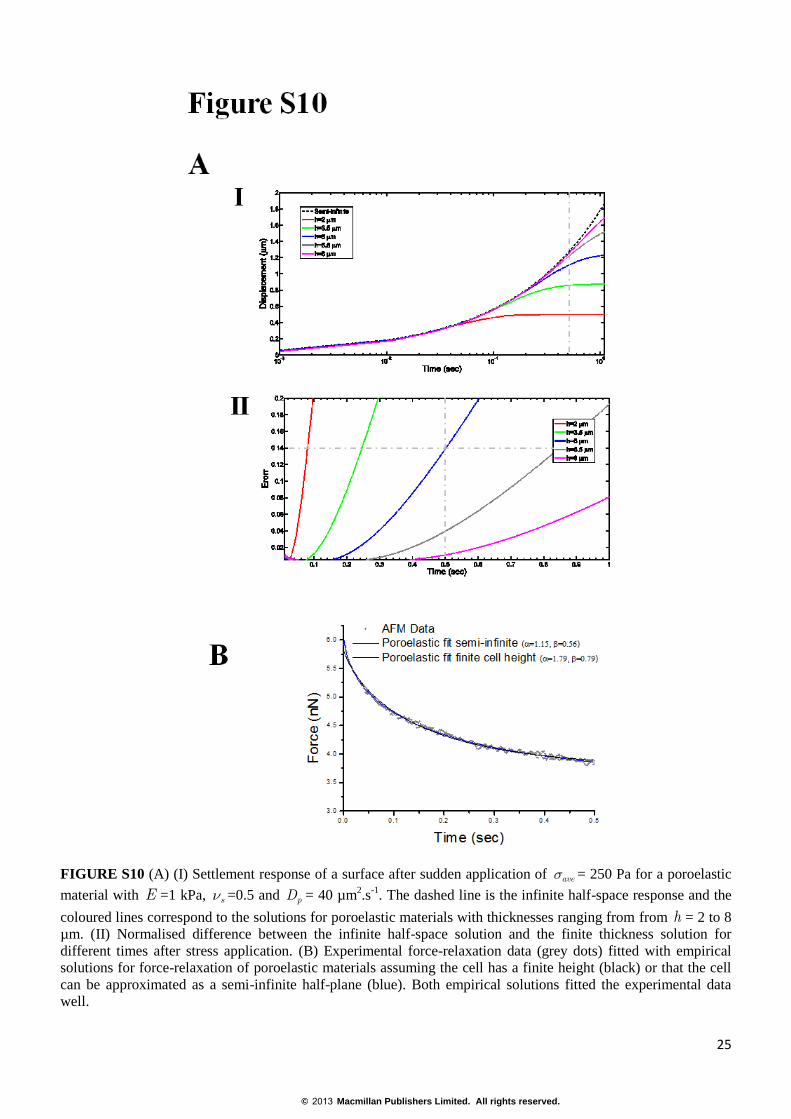
Effects of finite cell height. To extract the poroelastic diffusion constant from experimental data, we utilised the
finite-element approximation derived by Hu et al. 22
. In this study, the thickness of the poroelastic material was
assumed to be infinite. At short times after the start of relaxation, the infinite half-space solution is applicable for
materials of finite thickness. To investigate the precision of short time-scale approximations, we made the
simplifying assumption that to the first order indentation can be considered analogous to a one dimensional
consolidation. With this assumption, sudden application of a surface stress 0s gives rise to the following
displacement fields in a finite domain of length h and in an infinite half-space respectively 1,21
:
2 20 2 2 2
1,3,..
( , )(1 2 ) 8
cos 1 exp ,2 (1 ) 2 4
ps
s s n
u x tD tL n x
nG n h h
n ps p
n p (13)
2
40
(1 2 )( , ) 2 .
2 (1 ) 2p
xs D t
s s p
Dt xu x t e xerfc
G D tn
sn p
(14)
We utilise these exact solutions to investigate the time-scales over which we can employ the half-space
approximation in a material of finite thickness. In our experiments, application of F ~ 6 nN via a spherical tip of
radius R = 7.5 µm resulted in indentation depths of 0d ~1 µm leading to average stresses of /ave F Rs p d ~
250 Pa. Fig. S10A-I shows the surface displacements as a function of time for various cell thicknesses (from h =
2 to 8 µm) compared to the displacements in an infinite half-space. Comparing the finite and infinite thickness
solutions, we find that for cell thicknesses of h ~5 µm (comparable to our experimental measurements of the
height of HeLa cells) the infinite half-space solution is a good approximation for times shorter than 0.5s (less than
15% error, Fig. S10A-II). Hence, fitting our experimental data for time-scales shorter than 0.5s with the infinite
half-space solution provides an acceptable approximation.
Recently, detailed finite-element simulations of indentation of thin layers of poroelastic materials20
have shown
that force-relaxation can be approximated in terms of stretched exponential functions: [F(t)-Ff]/[Fi-Ff ]=exp(-ατβ)
where α and β are functions estimated empirically from the simulations that depend on the characteristic length of
the problem RL d and the height h of the layer:
2 3 4
2 3 4 5
1.15 0.44( / ) 0.89( / ) 0.42( / ) 0.06( / )
0.56 0.25( / ) 0.28( / ) 0.31( / ) 0.1( / ) 0.01( / ) .R h R h R h R h
R h R h R h R h R h
a d d d d
b d d d d d (15)
In our experiments, we measured a height h~4.5µm for HeLa cells and estimated α and β from the above
equations. Fitting experimental force curves with the proposed stretched exponential function indicated that for
h>4.5µm and δ<1.4µm, approximating the cell to an infinite half-plane resulted in a less than 25% overestimation
of the poroelastic diffusion constant Dp (Fig. S10B).
Rescaling of relaxation curves. To gain further insight into the nature of cellular force-relaxation at short time-
scales, we acquired experimental relaxation curves following indentations with increasing depths. To analyse
these experiments, we selected cells with identical elasticities such that application of a chosen target force
resulted in identical indentation depths and we averaged their relaxation curves. This filtering procedure ensured
that the cellular relaxation curves were comparable in all aspects (Fig. S1A, S2A) and allowed us to assess
whether or not cellular relaxation was dependent upon indentation depth. Indeed, one hallmark of poroelastic
materials is that their characteristic relaxation time is length-scale dependent in contrast to power law relaxations
of the form (F(t)~F0(t/t0)β) and exponential relaxations of the form (F(t)~F0exp(-t/τ)) with β and τ indentation
depth independent parameters. For ideal stress-relaxations of any power-law or linear viscoelastic material,
normalisation of force between any arbitrarily chosen times t1 and t2 [F(t)-F(t1)]/[F(t2)-F(t1)] should lead to
© 2013 Macmillan Publishers Limited. All rights reserved.
9
collapse of all experimental relaxation curves onto one master curve. After force normalisation, experimental
force-relaxation curves acquired on cells for different indentation depths collapsed for times longer than ~1s but
were significantly different from one another for shorter times (Fig. S1B-C for MDCK cells and Fig. S2B for
HeLa cells), suggesting that, at short times, relaxation is length-scale dependent consistent with a poroelastic
behaviour.
Next, we considered the indentation of well-characterised poroelastic materials and examined if, at short times,
force-relaxation curves collapse onto one master curve following normalisation of force and rescaling of time with
respect to indentation depth (t/𝛿). To assess this, experimental curves must first be normalised such that force
relaxes between 1 and 0 using
( ) ( *)
( 0) ( *)F t F t tF t F t t
(16)
and then time must be rescaled with respect to indentation depth (t/δ). For physical hydrogels, all experimental
force-relaxation curves reach a plateau (F∞) after t=t∞ (Fig. S3A) and thus any time t*>t∞ is a suitable choice for
the normalisation of force (Fig. S3E). Subsequent rescaling of time with respect to indentation depth (t/𝛿) leads to
collapse of all experimental curves onto one master curve (Fig. S3F). To obtain collapse onto a master curve for
t*<t∞, t* must be selected proportional to the indentation depth 𝛿 specific to each curve: t*=α𝛿 where α (with
unit of s.μm-1
) is an arbitrary number fixed for all curves (Fig. S3C,D).
For cells, experimental force-relaxation curves do not reach a plateau because relaxation follows a power law at
long time-scales (Fig. 1D-II). Hence, to determine if relaxation displayed a poroelastic behaviour at short time-
scales, we followed the force normalisation and time rescaling steps described above for cases where t*<t∞.
These procedures resulted in all cellular force-relaxation curves collapsing onto a single master curve (Fig. S1E,
Fig. S2D). This behaviour was apparent in poroelastic hydrogels for both long and short time-scales (Fig. S3D,F)
and in cells for times shorter than ~0.5s (Fig. S1E, Fig. S2D). Taken together, these data suggested that at short
time-scales cellular relaxation is indentation depth dependent and therefore that cells behaved as poroelastic
materials.
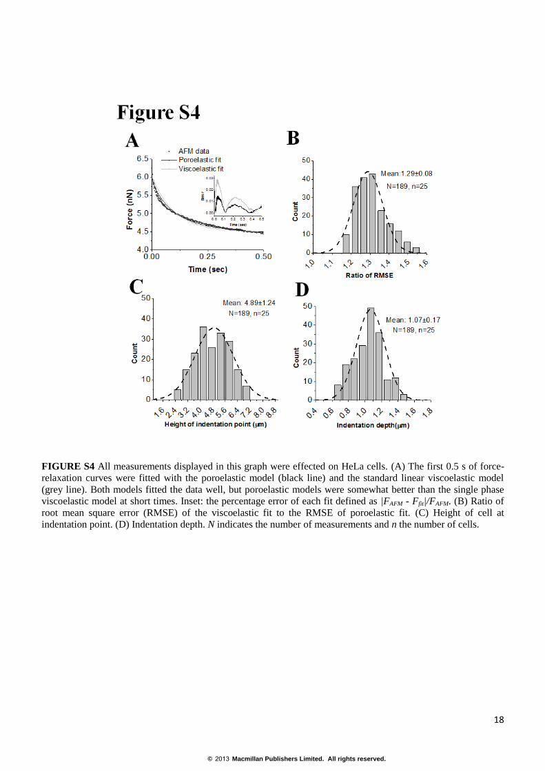
Apparent viscosity of the cytoplasm. To measure the apparent viscosity of the cytoplasm, we fitted force-
relaxation curves with (F(t)~e-k1t/η). Using the approach phase of AFM indentation curves we can measure
cellular elasticity and therefore the relaxations predicted by a viscoelastic formulation depend on only one free
parameter: the apparent viscosity η. Viscoelastic formulations were found to replicate experimental force-
relaxation curves well (on average r
2=0.92), but the early phase of force-relaxation was fit somewhat less
accurately by viscoelastic models (gray line, Fig. S4A) compared to poroelastic fits (black line, Fig. S4A). Indeed,
viscoelastic models gave rise to somewhat larger errors than poroelastic models (Fig. S4A). For HeLa cells, we
measured an average apparent viscosity of η=166±81 Pa.s. For HT1080 cells, we found an apparent viscosity
η=77±37 Pa.s, and for MDCK cells, η=50±15 Pa.s.
Estimation of the hydraulic pore size from experimental measurements of Dp. Using equations (7) and (8)
together with our experimental measurements of Dp (~40µm2.s
-1), E (~1 kPa), νs (~0.3), and the fluid fraction φ
(~0.75), we can estimate the hydraulic pore size numerically assuming k ~4, its lower bound for a random
distribution of particulate spheres for φ~0.75 31
. These values yield an estimate of ~0.05 for α in isotonic
conditions. Multiple experimental reports have shown that for small molecules the viscosity µ of the fluid-phase
of cytoplasm (cytosol) is 2-3 fold higher in cells than in aqueous media 32,33
. Using these values in equation (7)
yields a hydraulic pore size ξ of ~ 15 nm, comparable to the hydrodynamic radius of qdots with their PEG-
passivation layer 34
.
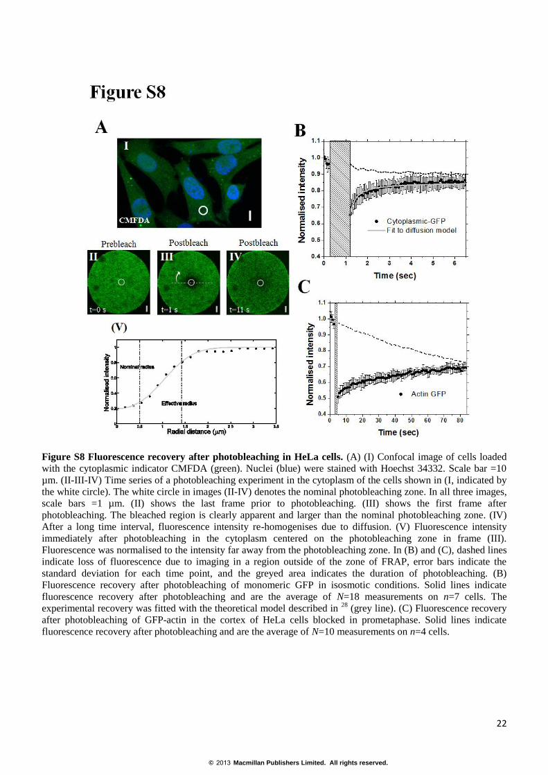
Effective bleach radius in FRAP experiments. To derive quantitative measurements of the translational
diffusion constants of molecules within the cytoplasm using the methods described in 28
, we experimentally
determined the effective bleach radius for a nominal bleaching zone of diameter 0.5 µm in the first post-bleach
image (Fig. S8A-III). Averaging over all diameters passing through the centre of the nominal bleach regions
© 2013 Macmillan Publishers Limited. All rights reserved.
10
yielded an experimental curve that could be fit with equation (11) to find re=1.5±0.2 µm (S5A-V, N=6
measurements on n=6 cells).
Measurement of translational diffusion constants in cells. Using the analytical procedures described in
supplementary methods, the estimated translational diffusion constant for CMFDA was DT, CMFDA=38.3±8 µm2.s
-1
(N=19 measurements on n=7 cells) in good agreement with published values in cells (Fig. 3B, DT=24-40 µm2.s
-1,
35) and 6 fold slower than in aqueous conditions (DT, CMFDA, aqueous=240 µm
2.s
-1
35) also consistent with previous
reports 35
. For GFP freely diffusing in the cytoplasm, we found DT,GFP=24.9±7 µm2.s
-1 (Fig. S8B, N=18
measurements on n=7 cells), consistent with values reported by others 28
. It should be noted that with CMFDA
loss of fluorescence due to imaging is very high (also reported by others, Fig. 3B). Therefore, we only utilised
data points up to a total fluorescence loss of 15% due to imaging to estimate the translational diffusion of
fluorophores in cells in normal isotonic condition. To estimate the reduction in translational diffusion of CMFDA
in cells under hyperosmotic conditions, we normalised the data following the procedures described in 36
and this
gave an estimated DT, CMFDA, Hyper=14 µm2.s
-1 (N=20 measurements on n=5 cells) ~3 fold lower than in isoosmotic
conditions.
Table S1 Effects of osmotic perturbations on translational diffusion coefficients DT (µm2.s
-1)
CMFDA-Control
N=19, n=7
CMFDA-PEG-400
N=20, n=5
EGFP10x-Control
N=17, n=6
EGFP10x-Water+N+D
N=23, n=7
38.3±8 13.7±4 8.6±2 15.5±5
Estimation of cortical F-actin turnover half-time. To assess the turnover rate of the F-actin cytoskeleton, HeLa
cells stably expressing actin-GFP were blocked in prometaphase by overnight treatment with 100 nM nocodazole.
Under these conditions, cells form a well-defined actin cortex. To estimate F-actin turnover, photobleaching was
performed on the F-actin cortex and recovery was imaged at a frame rate of 0.9s/frame (Fig. S8C). We obtained a
half time recovery of t1/2, F-actin=11.2±3 s (N=10 measurements on n=4 cells).
Spatial variations in poroelastic properties. Maps of cellular elasticity measured by AFM show that E is
strongly dependent upon location within the cell with actin-rich organelles (lamellipodium, actin stress fibres)
appearing significantly stiffer than other parts of the cell 37
. Hence, we asked if something similar could be
observed for poroelastic properties by measuring these at different locations along the cell long axis (Fig. S9A).
We performed N=386 total measurements on n=30 cells and displayed the measurements averaged over 2 µm
bins as a function of distance to the centroid of the nucleus. Cell height decreased significantly with increasing
distance from the nucleus (Fig. S9B) and this measurement enabled us to exclude low areas of the cell that are
prone to measurement artefacts due to limited thickness. The poroelastic diffusion constant Dp decreased slightly,
but not significantly, away from the nucleus decreasing from 40 µm2.s
-1 to ~30 µm
2.s
-1 (p>0.02, Fig. S9D). In
contrast, elasticity increased significantly away from the nucleus increasing from ~500 Pa to ~1200 Pa in lower
areas (Fig. S9C). Finally, the lumped pore size estimated from the ratio (Dpμ/E)1/2
also decreased significantly
away from the nucleus (Fig. S9E).
© 2013 Macmillan Publishers Limited. All rights reserved.
11
DISCUSSION
A length-scale dependent effective cellular viscosity. At time-scales short compared to 1s, force-relaxation
decays exponentially in poroelastic models as it does in simple Maxwell models of the cytoplasm (Supplementary
Results), but with the important difference that the Maxwell model makes no distinction between shear and
dilatation, and has no microstructural basis in terms of the two phase picture of a fluid bathed network. However,
in the context of observations past and present, this does suggest the following relationship for a length-scale
dependent effective cellular viscosity η
2
,L
h mx
(17)
with L a characteristic length-scale and μ the viscosity of cytosol. Given the dependence of η on the ratio of a
mesoscopic length-scale to a microscopic length-scale in the system may explain the large spread in reported
measurements of cytoplasmic viscosities 38,39
.
Poroelasticity in physiological cell shape changes and tissue deformations. To gain an understanding of how
widespread poroelastic effects are in the rheology of isolated cells and cells within tissues, one can compute the
poroelastic Péclet number Pe=(VL)/Dp, with V a characteristic velocity (due to active movement, external loading,
etc). For Pe >> 1, poroelastic effects dominate the viscoelastic response of the cytoplasm to shape change due to
externally applied loading or intrinsic cellular forces. In isolated cells, poroelastic effects have been implicated in
the formation of protrusions such as lamellipodia or blebs40
. For these, the rate of protrusion growth can be chosen
as a characteristic velocity. In rapidly moving cells, forward-directed intracellular water flows41,42
resulting from
pressure gradients due to myosin contraction of the cell rear have been proposed to participate in lamellipodial
protrusion42
. Assuming a representative lamellipodium length of L~10 µm and protrusion velocities of V~0.3
µm.s-1
, poroelastic effects will play an important role if Dp≤3 µm2.s
-1, lower than measured in the cytoplasm but
consistent with the far higher F-actin density observed in electron micrographs of the lamellipodium43
.
Furthermore, cells can also migrate using blebbing motility44
where large quasi-spherical blebs (L~10µm) arise at
the cell front with protrusion rates of V~1 µm.s-1
giving an estimate of Dp~10 µm2.s
-1 (comparable to the values
reported here) to obtain Pe≥1. During normal physiological function, cells within tissues of the respiratory and
cardiovascular systems are subjected to strains ε>20% applied at strain rates εt>20%.s-1
. As a first approximation,
we assume that these cells, with a representative length Lcell, undergo a length change L~εLcell applied with a
characteristic velocity V~Lcellεt. For cells within the lung alveola45
, Lcell~30 µm, ε~20%, εt~20%.s-1
and assuming
Dp~10 µm2.s
-1 (based on our measurements), we find Pe~3. Hence, these simple estimates of Pe suggest that water
redistribution participates in setting the rheology of cells within tissues under normal physiological conditions.
© 2013 Macmillan Publishers Limited. All rights reserved.
12
References:
1 Detournay, E. & Cheng, A. H. D. Fundamentals of poroelasticity. Comprehensive rock engineering 2, 113-171 (1993).
2 Biot, M. A. General theory of three-dimensional consolidation. Journal of applied physics 12, 155 (1941). 3 Mow, V. C., Kuei, S. C., Lai, W. M. & Armstrong, C. G. Biphasic creep and stress relaxation of articular
cartilage in compression: theory and experiments. Journal of biomechanical engineering 102, 73 (1980). 4 Scheidegger, A. E. The physics of flow through porous media. Soil Science 86, 355 (1958). 5 Ory, D. S., Neugeboren, B. A. & Mulligan, R. C. A stable human-derived packaging cell line for production
of high titer retrovirus/vesicular stomatitis virus G pseudotypes. Proceedings of the National Academy of Sciences of the United States of America 93, 11400 (1996).
6 Riedl, J. et al. Lifeact: a versatile marker to visualize F-actin. Nature methods 5, 605-607 (2008). 7 Bancaud, A. et al. Molecular crowding affects diffusion and binding of nuclear proteins in
heterochromatin and reveals the fractal organization of chromatin. The EMBO journal 28, 3785-3798 (2009).
8 Moulding, D. A. et al. Unregulated actin polymerization by WASp causes defects of mitosis and cytokinesis in X-linked neutropenia. The Journal of experimental medicine 204, 2213 (2007).
9 Demaison, C. et al. High-level transduction and gene expression in hematopoietic repopulating cells using a human imunodeficiency virus type 1-based lentiviral vector containing an internal spleen focus forming virus promoter. Human gene therapy 13, 803-813 (2002).
10 Zheng, Y., Wong, M. L., Alberts, B. & Mitchison, T. Nucleation of microtubule assembly by a gamma-tubulin-containing ring complex. Nature 378, 578-583 (1995).
11 Keppler, A. & Ellenberg, J. Chromophore-assisted laser inactivation of -and -tubulin SNAP-tag fusion proteins inside living cells. ACS Chemical Biology 4, 127-138 (2009).
12 Werner, N. S. et al. Epidermolysis bullosa simplex-type mutations alter the dynamics of the keratin cytoskeleton and reveal a contribution of actin to the transport of keratin subunits. Molecular biology of the cell 15, 990 (2004).
13 Zhou, E. H. et al. Universal behavior of the osmotically compressed cell and its analogy to the colloidal glass transition. Proceedings of the National Academy of Sciences 106, 10632 (2009).
14 Hoffmann, E. K., Lambert, I. H. & Pedersen, S. F. Physiology of cell volume regulation in vertebrates. Physiological reviews 89, 193 (2009).
15 Lin, D. C., Dimitriadis, E. K. & Horkay, F. Robust strategies for automated AFM force curve analysis—I. Non-adhesive indentation of soft, inhomogeneous materials. Journal of biomechanical engineering 129, 430 (2007).
16 Harris, A. R. & Charras, G. Experimental validation of atomic force microscopy-based cell elasticity measurements. Nanotechnology 22, 345102 (2011).
17 Johnson, K. L. Contact mechanics. (Cambridge university press, 1987). 18 Dimitriadis, E. K., Horkay, F., Maresca, J., Kachar, B. & Chadwick, R. S. Determination of elastic moduli of
thin layers of soft material using the atomic force microscope. Biophysical Journal 82, 2798-2810 (2002). 19 Charras, G. T., Lehenkari, P. P. & Horton, M. A. Atomic force microscopy can be used to mechanically
stimulate osteoblasts and evaluate cellular strain distributions. Ultramicroscopy 86, 85-95 (2001). 20 Chan, E. P., Hu, Y., Johnson, P. M., Suo, Z. & Stafford, C. M. Spherical indentation testing of poroelastic
relaxations in thin hydrogel layers. Soft Matter 8, 1492-1498 (2012). 21 Wang, H. Theory of linear poroelasticity: with applications to geomechanics and hydrogeology.
(Princeton Univ Pr, 2000). 22 Hu, Y., Zhao, X., Vlassak, J. J. & Suo, Z. Using indentation to characterize the poroelasticity of gels.
Applied Physics Letters 96, 121904 (2010). 23 Galli, M., Oyen, M. L. & Source, C. Fast Identification of Poroelastic Parameters from Indentation Tests.
Computer Modeling in Engineering and Science 48, 241-270 (2009). 24 Charras, G. T., Mitchison, T. J. & Mahadevan, L. Animal cell hydraulics. Journal of Cell Science 122, 3233
(2009).
© 2013 Macmillan Publishers Limited. All rights reserved.
13
25 Mitchison, T. J., Charras, G. T. & Mahadevan, L. 215-223 (Elsevier). 26 Darling, E. M., Zauscher, S. & Guilak, F. Viscoelastic properties of zonal articular chondrocytes measured
by atomic force microscopy. Osteoarthritis and Cartilage 14, 571-579 (2006). 27 Charras, G. T., Hu, C. K., Coughlin, M. & Mitchison, T. J. Reassembly of contractile actin cortex in cell
blebs. The Journal of cell biology 175, 477-490 (2006). 28 Kang, M., Day, C. A., Drake, K., Kenworthy, A. K. & DiBenedetto, E. A generalization of theory for two-
dimensional fluorescence recovery after photobleaching applicable to confocal laser scanning microscopes. Biophysical Journal 97, 1501-1511 (2009).
29 Axelrod, D., Koppel, D. E., Schlessinger, J., Elson, E. & Webb, W. W. Mobility measurement by analysis of fluorescence photobleaching recovery kinetics. Biophysical Journal 16, 1055-1069 (1976).
30 Soumpasis, D. M. Theoretical analysis of fluorescence photobleaching recovery experiments. Biophysical Journal 41, 95-97 (1983).
31 Happel, J. & Brenner, H. Low Reynolds number hydrodynamics: with special applications to particulate media. Vol. 1 (Springer, 1983).
32 Mastro, A. M., Babich, M. A., Taylor, W. D. & Keith, A. D. Diffusion of a small molecule in the cytoplasm of mammalian cells. Proceedings of the National Academy of Sciences 81, 3414 (1984).
33 Persson, E. & Halle, B. Cell water dynamics on multiple time scales. Proceedings of the National Academy of Sciences 105, 6266 (2008).
34 Derfus, A. M., Chan, W. C. W. & Bhatia, S. N. Intracellular delivery of quantum dots for live cell labeling and organelle tracking. Advanced Materials 16, 961-966 (2004).
35 Swaminathan, R., Bicknese, S., Periasamy, N. & Verkman, A. S. Cytoplasmic viscosity near the cell plasma membrane. Biophysical Journal 71, 1140-1151 (1996).
36 Phair, R. D. & Misteli, T. High mobility of proteins in the mammalian cell nucleus. Nature 404, 604-608 (2000).
37 Rotsch, C. & Radmacher, M. Drug-induced changes of cytoskeletal structure and mechanics in fibroblasts: an atomic force microscopy study. Biophys J 78, 520-535 (2000).
38 Bausch, A. R., Möller, W. & Sackmann, E. Measurement of local viscoelasticity and forces in living cells by magnetic tweezers. Biophysical journal 76, 573-579 (1999).
39 Hoffman, B. D. & Crocker, J. C. Cell mechanics: dissecting the physical responses of cells to force. Annual review of biomedical engineering 11, 259-288 (2009).
40 Charras, G. T., Yarrow, J. C., Horton, M. A., Mahadevan, L. & Mitchison, T. J. Non-equilibration of hydrostatic pressure in blebbing cells. Nature 435, 365-369 (2005).
41 Zicha, D. et al. Rapid actin transport during cell protrusion. Science 300, 142-145 (2003). 42 Keren, K., Yam, P. T., Kinkhabwala, A., Mogilner, A. & Theriot, J. A. Intracellular fluid flow in rapidly
moving cells. Nature cell biology 11, 1219-1224 (2009). 43 Pollard, T. D. & Borisy, G. G. Cellular motility driven by assembly and disassembly of actin filaments. Cell
112, 453-465 (2003). 44 Charras, G. & Paluch, E. Blebs lead the way: how to migrate without lamellipodia. Nature Reviews
Molecular Cell Biology 9, 730-736 (2008). 45 Perlman, C. E. & Bhattacharya, J. Alveolar expansion imaged by optical sectioning microscopy. Journal of
applied physiology 103, 1037-1044 (2007).
© 2013 Macmillan Publishers Limited. All rights reserved.

14
SUPPLEMENTARY MOVIE
Movement of PEG-passivated quantum dots microinjected in a HeLa cell in isoosmotic conditions (left) and in
hyperosmotic conditions (right). Both movies are 120 frames long totalling 18 s and are single confocal sections.
In isoosmotic conditions, quantum dots move freely (left); whereas in hyperosmotic conditions, quantum dots are
immobile because they are trapped within the cytoplasmic mesh (right). Scale bars =10 μm.
© 2013 Macmillan Publishers Limited. All rights reserved.
15
SUPPLEMENTARY FIGURES
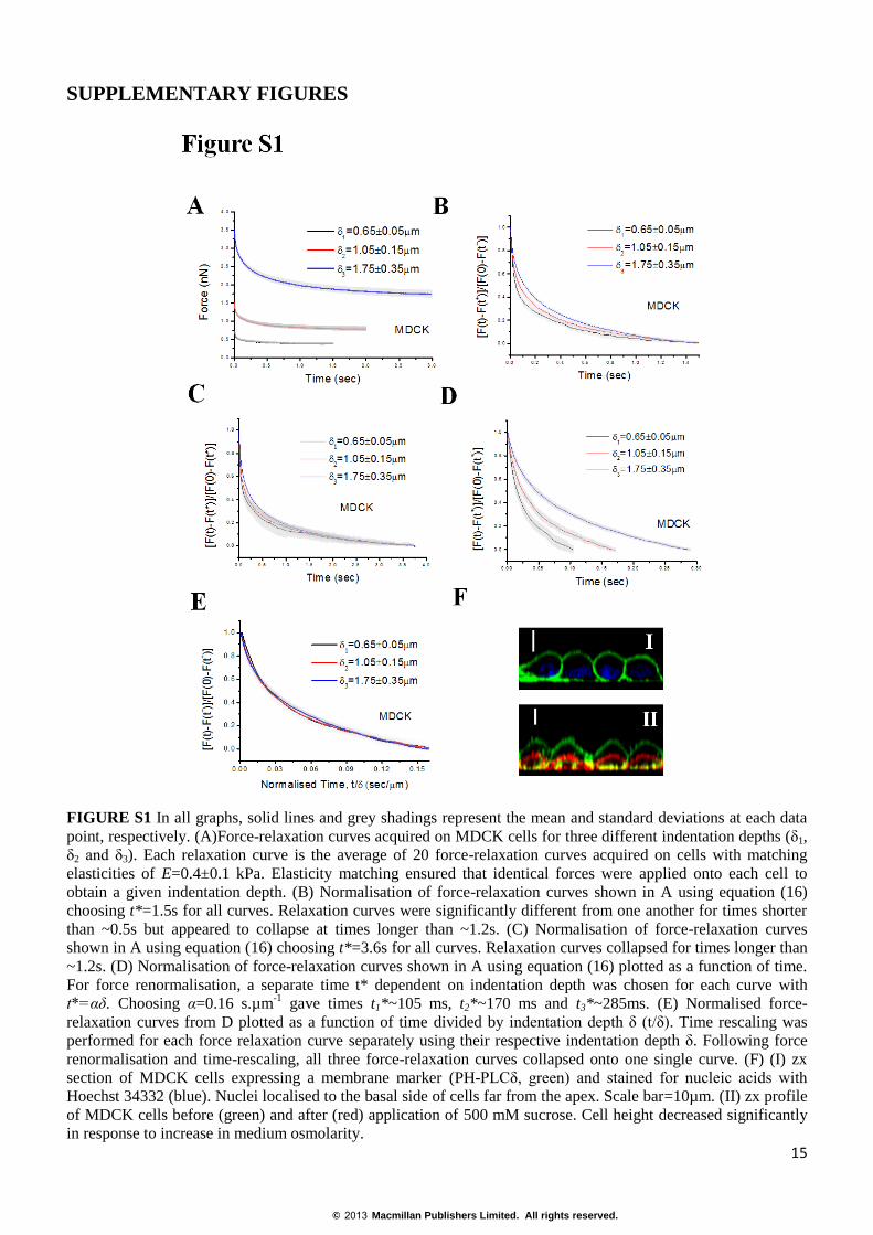
FIGURE S1 In all graphs, solid lines and grey shadings represent the mean and standard deviations at each data
point, respectively. (A)Force-relaxation curves acquired on MDCK cells for three different indentation depths (δ1,
δ2 and δ3). Each relaxation curve is the average of 20 force-relaxation curves acquired on cells with matching
elasticities of E=0.4±0.1 kPa. Elasticity matching ensured that identical forces were applied onto each cell to
obtain a given indentation depth. (B) Normalisation of force-relaxation curves shown in A using equation (16)
choosing t*=1.5s for all curves. Relaxation curves were significantly different from one another for times shorter
than ~0.5s but appeared to collapse at times longer than ~1.2s. (C) Normalisation of force-relaxation curves
shown in A using equation (16) choosing t*=3.6s for all curves. Relaxation curves collapsed for times longer than
~1.2s. (D) Normalisation of force-relaxation curves shown in A using equation (16) plotted as a function of time.
For force renormalisation, a separate time t* dependent on indentation depth was chosen for each curve with
t*=αδ. Choosing α=0.16 s.µm-1
gave times t1*~105 ms, t2*~170 ms and t3*~285ms. (E) Normalised force-
relaxation curves from D plotted as a function of time divided by indentation depth δ (t/δ). Time rescaling was
performed for each force relaxation curve separately using their respective indentation depth δ. Following force
renormalisation and time-rescaling, all three force-relaxation curves collapsed onto one single curve. (F) (I) zx
section of MDCK cells expressing a membrane marker (PH-PLCδ, green) and stained for nucleic acids with
Hoechst 34332 (blue). Nuclei localised to the basal side of cells far from the apex. Scale bar=10µm. (II) zx profile
of MDCK cells before (green) and after (red) application of 500 mM sucrose. Cell height decreased significantly
in response to increase in medium osmolarity.
© 2013 Macmillan Publishers Limited. All rights reserved.
16
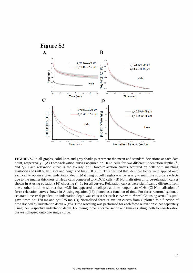
FIGURE S2 In all graphs, solid lines and grey shadings represent the mean and standard deviations at each data
point, respectively. (A) Force-relaxation curves acquired on HeLa cells for two different indentation depths (δ1
and δ2). Each relaxation curve is the average of 5 force-relaxation curves acquired on cells with matching
elasticities of E=0.66±0.1 kPa and heights of h=5.5±0.3 μm. This ensured that identical forces were applied onto
each cell to obtain a given indentation depth. Matching of cell heights was necessary to minimise substrate effects
due to the smaller thickness of HeLa cells compared to MDCK cells. (B) Normalisation of force-relaxation curves
shown in A using equation (16) choosing t*=1s for all curves. Relaxation curves were significantly different from
one another for times shorter than ~0.5s but appeared to collapse at times longer than ~0.6s. (C) Normalisation of
force-relaxation curves shown in A using equation (16) plotted as a function of time. For force renormalisation, a
separate time t* dependent on indentation depth was chosen for each curve with t*=αδ. Choosing α=0.19 s.µm-1
gave times t1*~170 ms and t2*~275 ms. (D) Normalised force-relaxation curves from C plotted as a function of
time divided by indentation depth δ (t/δ). Time rescaling was performed for each force relaxation curve separately
using their respective indentation depth. Following force renormalisation and time-rescaling, both force-relaxation
curves collapsed onto one single curve.
© 2013 Macmillan Publishers Limited. All rights reserved.
17
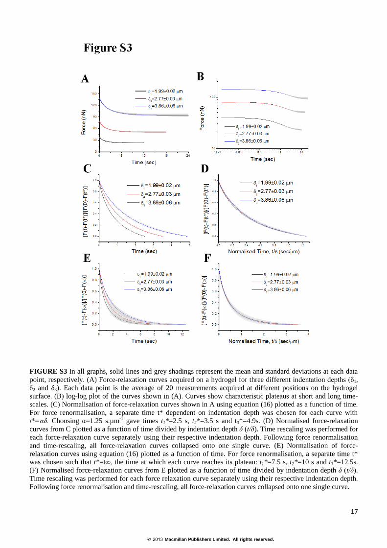
FIGURE S3 In all graphs, solid lines and grey shadings represent the mean and standard deviations at each data
point, respectively. (A) Force-relaxation curves acquired on a hydrogel for three different indentation depths (δ1,
δ2 and δ3). Each data point is the average of 20 measurements acquired at different positions on the hydrogel
surface. (B) log-log plot of the curves shown in (A). Curves show characteristic plateaus at short and long time-
scales. (C) Normalisation of force-relaxation curves shown in A using equation (16) plotted as a function of time.
For force renormalisation, a separate time t* dependent on indentation depth was chosen for each curve with
t*=αδ. Choosing α=1.25 s.µm-1
gave times t1*=2.5 s, t2*=3.5 s and t3*=4.9s. (D) Normalised force-relaxation
curves from C plotted as a function of time divided by indentation depth δ (t/δ). Time rescaling was performed for
each force-relaxation curve separately using their respective indentation depth. Following force renormalisation
and time-rescaling, all force-relaxation curves collapsed onto one single curve. (E) Normalisation of force-
relaxation curves using equation (16) plotted as a function of time. For force renormalisation, a separate time t*
was chosen such that t*=t∞, the time at which each curve reaches its plateau: t1*=7.5 s, t2*=10 s and t3*=12.5s.
(F) Normalised force-relaxation curves from E plotted as a function of time divided by indentation depth δ (t/δ).
Time rescaling was performed for each force relaxation curve separately using their respective indentation depth.
Following force renormalisation and time-rescaling, all force-relaxation curves collapsed onto one single curve.
© 2013 Macmillan Publishers Limited. All rights reserved.
18
FIGURE S4 All measurements displayed in this graph were effected on HeLa cells. (A) The first 0.5 s of force-
relaxation curves were fitted with the poroelastic model (black line) and the standard linear viscoelastic model
(grey line). Both models fitted the data well, but poroelastic models were somewhat better than the single phase
viscoelastic model at short times. Inset: the percentage error of each fit defined as |FAFM - Ffit|/FAFM. (B) Ratio of
root mean square error (RMSE) of the viscoelastic fit to the RMSE of poroelastic fit. (C) Height of cell at
indentation point. (D) Indentation depth. N indicates the number of measurements and n the number of cells.
© 2013 Macmillan Publishers Limited. All rights reserved.
19
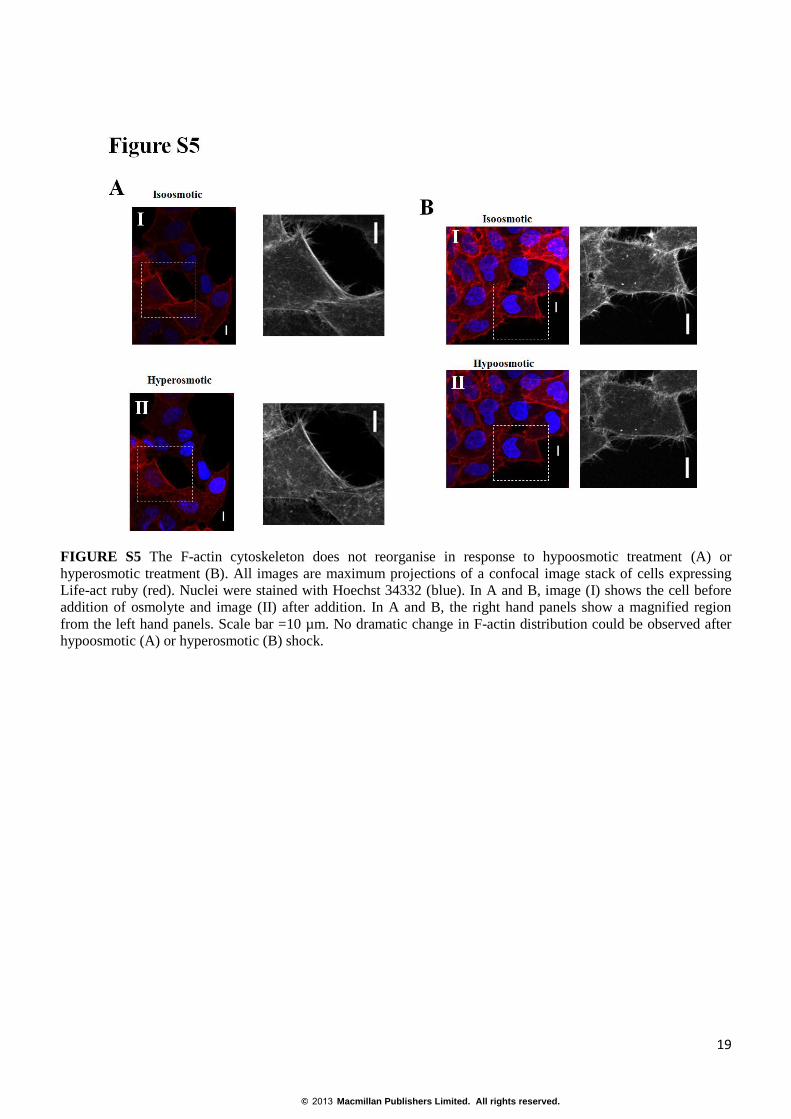
FIGURE S5 The F-actin cytoskeleton does not reorganise in response to hypoosmotic treatment (A) or
hyperosmotic treatment (B). All images are maximum projections of a confocal image stack of cells expressing
Life-act ruby (red). Nuclei were stained with Hoechst 34332 (blue). In A and B, image (I) shows the cell before
addition of osmolyte and image (II) after addition. In A and B, the right hand panels show a magnified region
from the left hand panels. Scale bar =10 µm. No dramatic change in F-actin distribution could be observed after
hypoosmotic (A) or hyperosmotic (B) shock.
© 2013 Macmillan Publishers Limited. All rights reserved.
20
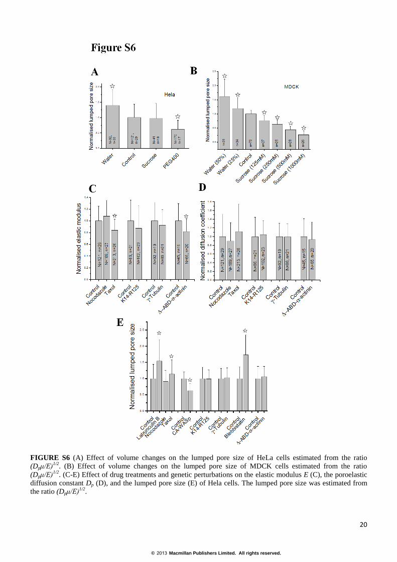
FIGURE S6 (A) Effect of volume changes on the lumped pore size of HeLa cells estimated from the ratio
(Dpμ/E)1/2
. (B) Effect of volume changes on the lumped pore size of MDCK cells estimated from the ratio
(Dpμ/E)1/2
. (C-E) Effect of drug treatments and genetic perturbations on the elastic modulus E (C), the poroelastic
diffusion constant Dp (D), and the lumped pore size (E) of Hela cells. The lumped pore size was estimated from
the ratio (Dpμ/E)1/2
.
© 2013 Macmillan Publishers Limited. All rights reserved.
21
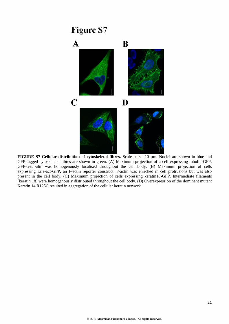
FIGURE S7 Cellular distribution of cytoskeletal fibres. Scale bars =10 µm. Nuclei are shown in blue and
GFP-tagged cytoskeletal fibres are shown in green. (A) Maximum projection of a cell expressing tubulin-GFP.
GFP-α-tubulin was homogenously localised throughout the cell body. (B) Maximum projection of cells
expressing Life-act-GFP, an F-actin reporter construct. F-actin was enriched in cell protrusions but was also
present in the cell body. (C) Maximum projection of cells expressing keratin18-GFP. Intermediate filaments
(keratin 18) were homogenously distributed throughout the cell body. (D) Overexpression of the dominant mutant
Keratin 14 R125C resulted in aggregation of the cellular keratin network.
© 2013 Macmillan Publishers Limited. All rights reserved.
22
Figure S8 Fluorescence recovery after photobleaching in HeLa cells. (A) (I) Confocal image of cells loaded
with the cytoplasmic indicator CMFDA (green). Nuclei (blue) were stained with Hoechst 34332. Scale bar =10
µm. (II-III-IV) Time series of a photobleaching experiment in the cytoplasm of the cells shown in (I, indicated by
the white circle). The white circle in images (II-IV) denotes the nominal photobleaching zone. In all three images,
scale bars =1 µm. (II) shows the last frame prior to photobleaching. (III) shows the first frame after
photobleaching. The bleached region is clearly apparent and larger than the nominal photobleaching zone. (IV)
After a long time interval, fluorescence intensity re-homogenises due to diffusion. (V) Fluorescence intensity
immediately after photobleaching in the cytoplasm centered on the photobleaching zone in frame (III).
Fluorescence was normalised to the intensity far away from the photobleaching zone. In (B) and (C), dashed lines
indicate loss of fluorescence due to imaging in a region outside of the zone of FRAP, error bars indicate the
standard deviation for each time point, and the greyed area indicates the duration of photobleaching. (B)
Fluorescence recovery after photobleaching of monomeric GFP in isosmotic conditions. Solid lines indicate
fluorescence recovery after photobleaching and are the average of N=18 measurements on n=7 cells. The
experimental recovery was fitted with the theoretical model described in 28
(grey line). (C) Fluorescence recovery
after photobleaching of GFP-actin in the cortex of HeLa cells blocked in prometaphase. Solid lines indicate
fluorescence recovery after photobleaching and are the average of N=10 measurements on n=4 cells.
© 2013 Macmillan Publishers Limited. All rights reserved.
23
© 2013 Macmillan Publishers Limited. All rights reserved.
24
FIGURE S9 Spatial distribution of cellular rheological properties. (A) Representative phase contrast image of
a HeLa cell and the location of AFM measurements on its surface (I). The position of the height reference, where
the AFM tip contacts the glass surface was also chosen as the xy reference (fluorescence image of the bead, IV).
The location of the nucleus was determined using Hoechst 34332 staining (III) and the centroid of the nucleus was
used as a reference for displaying data. To determine the exact pathline of the bead and to calculate the distance of
each point from the centre of nucleus, images of the cell (II), the cell nucleus (III), and the bead (IV) were
overlaid (I). Scale bars =10 μm. (B-E) Scatter plots of the average cell height, poroelastic diffusion constant,
elasticity, and lumped pore size as a function of distance to the centre of nucleus. Each scatter graph is generated
by averaging values of each variable over 2 μm wide bins. Filled black circles indicate locations above the
nucleus, white open circles in the cytoplasm, and grey filled circles boundary areas. The lines indicate the
weighted least-square fit of the scattered data. Open circles with a cross superimposed indicate measurements
significantly different (p<0.01) from those obtained above the nucleus.
© 2013 Macmillan Publishers Limited. All rights reserved.
25
FIGURE S10 (A) (I) Settlement response of a surface after sudden application of aves = 250 Pa for a poroelastic
material with E =1 kPa, sn =0.5 and pD = 40 µm2.s
-1. The dashed line is the infinite half-space response and the
coloured lines correspond to the solutions for poroelastic materials with thicknesses ranging from from h = 2 to 8
µm. (II) Normalised difference between the infinite half-space solution and the finite thickness solution for
different times after stress application. (B) Experimental force-relaxation data (grey dots) fitted with empirical
solutions for force-relaxation of poroelastic materials assuming the cell has a finite height (black) or that the cell
can be approximated as a semi-infinite half-plane (blue). Both empirical solutions fitted the experimental data
well.
© 2013 Macmillan Publishers Limited. All rights reserved.
Related Documents