Supplemental Article S1: Bonobo dissection and model ...

Supplemental Article S1:Bonobo dissection and model parameteracquisition

ABSTRACT

This supplemental article describes in more detail how the Bonobo dissection was conducted and howthe initial parameters of the bonobo model were acquired.

INTRODUCTIONAs mentioned in the main manuscript, initial parameters for the bonobo finger model were needed inanalogy to those of the human finger model available from literature (specifically from An et al. (1979)).This comprises the following data:

1. Finger segment lengths for the kinematic description

2. Via point coordinates of each muscle/tendon at each joint

3. Physiological cross sectional areas (PCSA) of each muscle

The respective parameters were obtained from a dissection study performed at the Jan Palfijn AnatomyLab of the KU Leuven and coordinated by Evie Vereecke. A bonobo specimen (8 years old; female; rightarm) was made available by the Antwerp Zoo by Centre for Research and Conservation, Royal ZoologicalSociety Antwerp (KMDA/RZSA) as part of the Bonobo Morphology Initiative 2016.

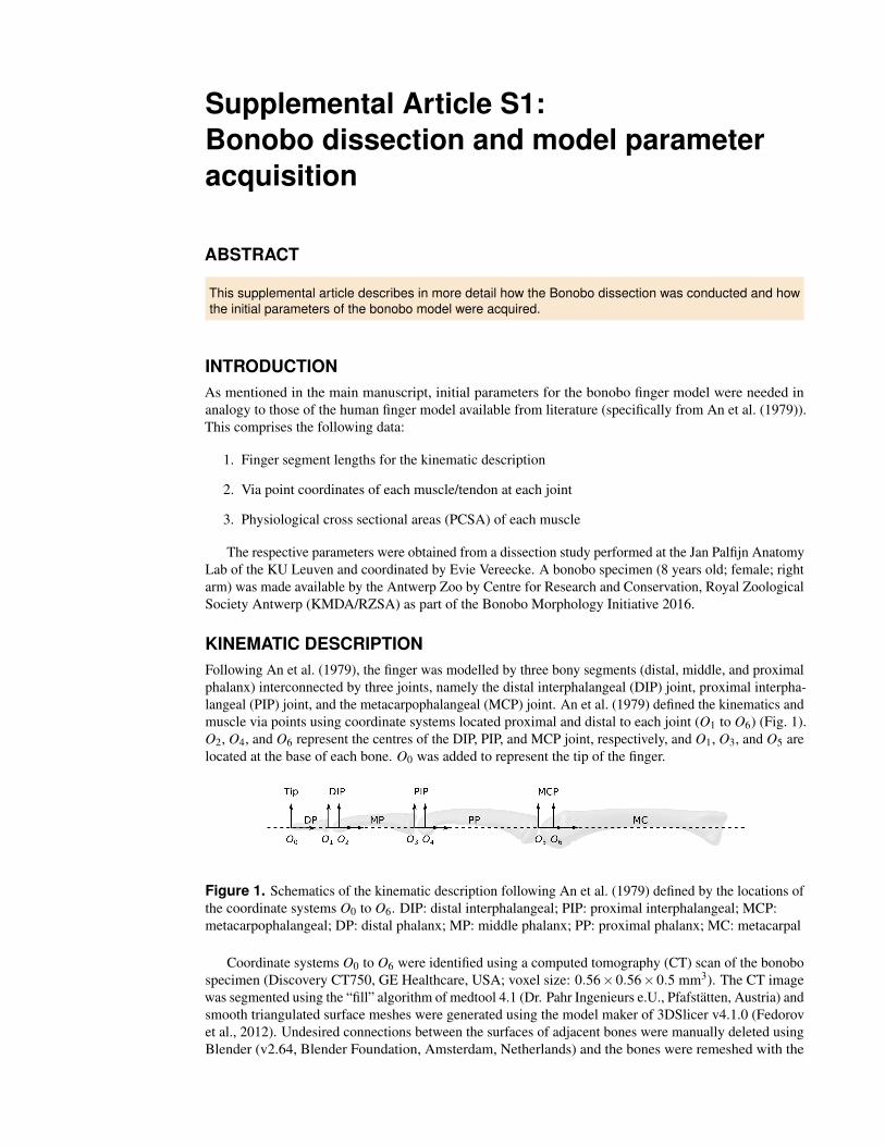
KINEMATIC DESCRIPTIONFollowing An et al. (1979), the finger was modelled by three bony segments (distal, middle, and proximalphalanx) interconnected by three joints, namely the distal interphalangeal (DIP) joint, proximal interpha-langeal (PIP) joint, and the metacarpophalangeal (MCP) joint. An et al. (1979) defined the kinematics andmuscle via points using coordinate systems located proximal and distal to each joint (O1 to O6) (Fig. 1).O2, O4, and O6 represent the centres of the DIP, PIP, and MCP joint, respectively, and O1, O3, and O5 arelocated at the base of each bone. O0 was added to represent the tip of the finger.

Figure 1. Schematics of the kinematic description following An et al. (1979) defined by the locations ofthe coordinate systems O0 to O6. DIP: distal interphalangeal; PIP: proximal interphalangeal; MCP:metacarpophalangeal; DP: distal phalanx; MP: middle phalanx; PP: proximal phalanx; MC: metacarpal

Coordinate systems O0 to O6 were identified using a computed tomography (CT) scan of the bonobospecimen (Discovery CT750, GE Healthcare, USA; voxel size: 0.56×0.56×0.5 mm3). The CT imagewas segmented using the “fill” algorithm of medtool 4.1 (Dr. Pahr Ingenieurs e.U., Pfafstatten, Austria) andsmooth triangulated surface meshes were generated using the model maker of 3DSlicer v4.1.0 (Fedorovet al., 2012). Undesired connections between the surfaces of adjacent bones were manually deleted usingBlender (v2.64, Blender Foundation, Amsterdam, Netherlands) and the bones were remeshed with the

“remesh modifier” of Blender to ensure all holes of the mesh were closed. The average edge length of thefinal triangulated meshes of all bones was 0.47 mm.

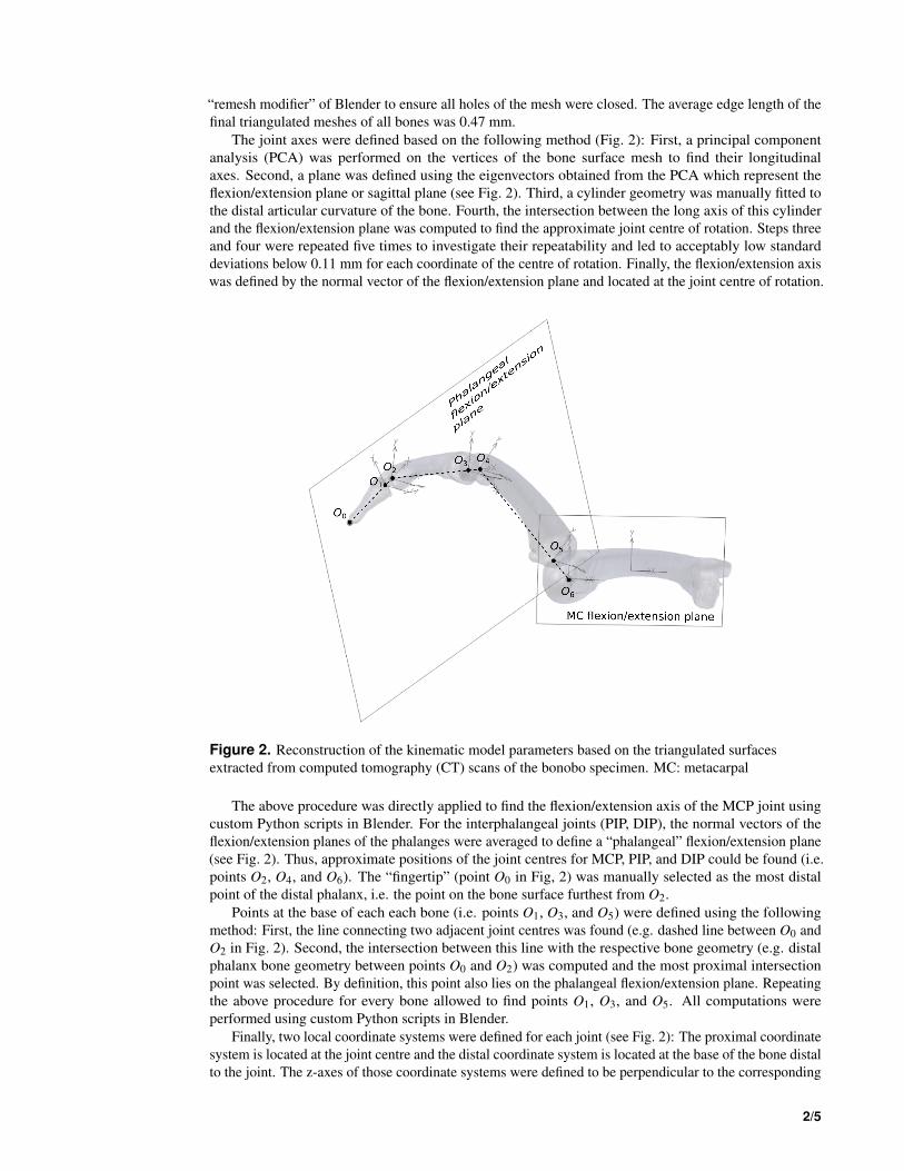
The joint axes were defined based on the following method (Fig. 2): First, a principal componentanalysis (PCA) was performed on the vertices of the bone surface mesh to find their longitudinalaxes. Second, a plane was defined using the eigenvectors obtained from the PCA which represent theflexion/extension plane or sagittal plane (see Fig. 2). Third, a cylinder geometry was manually fitted tothe distal articular curvature of the bone. Fourth, the intersection between the long axis of this cylinderand the flexion/extension plane was computed to find the approximate joint centre of rotation. Steps threeand four were repeated five times to investigate their repeatability and led to acceptably low standarddeviations below 0.11 mm for each coordinate of the centre of rotation. Finally, the flexion/extension axiswas defined by the normal vector of the flexion/extension plane and located at the joint centre of rotation.

Figure 2. Reconstruction of the kinematic model parameters based on the triangulated surfacesextracted from computed tomography (CT) scans of the bonobo specimen. MC: metacarpal

The above procedure was directly applied to find the flexion/extension axis of the MCP joint usingcustom Python scripts in Blender. For the interphalangeal joints (PIP, DIP), the normal vectors of theflexion/extension planes of the phalanges were averaged to define a “phalangeal” flexion/extension plane(see Fig. 2). Thus, approximate positions of the joint centres for MCP, PIP, and DIP could be found (i.e.points O2, O4, and O6). The “fingertip” (point O0 in Fig, 2) was manually selected as the most distalpoint of the distal phalanx, i.e. the point on the bone surface furthest from O2.

Points at the base of each each bone (i.e. points O1, O3, and O5) were defined using the followingmethod: First, the line connecting two adjacent joint centres was found (e.g. dashed line between O0 andO2 in Fig. 2). Second, the intersection between this line with the respective bone geometry (e.g. distalphalanx bone geometry between points O0 and O2) was computed and the most proximal intersectionpoint was selected. By definition, this point also lies on the phalangeal flexion/extension plane. Repeatingthe above procedure for every bone allowed to find points O1, O3, and O5. All computations wereperformed using custom Python scripts in Blender.

Finally, two local coordinate systems were defined for each joint (see Fig. 2): The proximal coordinatesystem is located at the joint centre and the distal coordinate system is located at the base of the bone distalto the joint. The z-axes of those coordinate systems were defined to be perpendicular to the corresponding

2/5

flexion/extension plane. The x-axes were defined to be aligned with the connection line between theorigin of the coordinate system Oi and point Oi+1. The locations of all coordinate systems of the thirddigit are displayed in Table 1. Values are presented both in absolute numbers and normalized to segmentO2O3 following An et al. (1979).

Segment O0O1 O1O2 O2O3 O3O4 O4O5 O5O6Length (mm) 17.54 3.30 33.91 5.09 49.08 10.00Normalized Length (-) 0.517 0.097 1.000 0.150 1.447 0.295

Table 1. Segment lengths defining the kinematics of the third digit of the bonobo, both in absolutevalues and normalized to O2O3. See Fig. 1 and 2 for a graphical representation of points O0 to O6.

MUSCLE/TENDON VIA POINTS

Following the definition of An et al. (1979), each muscle/tendon path needs to be defined by two via pointslocated proximally and distally with respect to each joint and expressed in proximal and distal coordinatesystem, respectively. In analogy to the human model, tendons of six muscles of the third digit wereincluded in the bonobo model: flexor digitorum profundus (FDP), flexor digitorum superficialis (FDS),extensor digitorum communis (EDC), lumbrical (LU), radial interosseus (RI), and ulnar interosseus (UI).Additionally, the via points of the extensor mechanism parts, namley radial band, ulnar band, central slip,and terminal slip were required.

The via points were recorded from the bonobo specimen using an electromagnetic six degrees offreedom (DoF) motion tracking system (Patriot, Polhemus, Vermont, USA). First, tendon path pointswere collected by digitizing points along the tendon at regular intervals (see Fig. 3). In order to obtaintendon path points for all muscles in common coordinate frames, the points were recorded relative tolandmarks placed on each bone. These landmarks were defined by four radio-opaque markers (garnetstones attached with bee’s wax, see Fig. 3, left) placed on each bone. Thus, the digitized landmarks couldbe registered to the landmarks identified in the CT scan (Fig. 3, right) and all tendon path points could betransformed into common, bone specific coordinate frames. The landmark registration was performedusing the method of Veldpaus et al. (1988) implemented with custom Python scripts.

Figure 3. Via point digitization and location of radio-opaque markers during dissection (left) and asidentified in the computed tomography scan (right). DP: distal phalanx; MP: middle phalanx; PP:proximal phalanx; MC: metacarpal

Finally, one proximal and one distal point of each tendon relative to each joint which best representedan anatomical constraint (e.g. pulley of a flexor tendon) were chosen and their positions were evaluated inthe respective coordinate systems. The resulting via point locations are displayed in Table 2 and Fig. 4.

3/5

Figure 4. 3D visualization of the tendon via points digitzed during the dissection and registered to thecomputed tomography (CT) scan. FDS: flexor digitorum superficialis; FDP: flexor digitorum profundus;RI: radial interosseus; UI: ulnar interosseus; LU: lumbrical; EDC: extensor digitorum communis

Joint Tendon Distal Point Proximal PointX Y Z X Y Z

DIP TS -0.177 0.085 -0.025 -0.024 0.052 -0.035FDP -0.056 -0.057 0.037 0.229 -0.084 0.033

PIP FDP -0.304 -0.122 0.091 0.101 -0.244 0.109RB -0.063 0.116 0.139 0.217 0.259 0.082UB -0.099 0.071 -0.223 0.253 0.205 -0.214FDS -0.348 -0.185 -0.057 0.105 -0.224 -0.020CS -0.129 0.142 -0.020 -0.022 0.198 -0.047

MCP FDP -0.192 -0.273 0.030 0.051 -0.346 -0.075FDS -0.277 -0.224 0.040 -0.036 -0.437 -0.074RI -0.219 -0.053 0.237 0.165 -0.208 0.164LU -0.160 -0.186 0.170 0.068 -0.455 0.042UI -0.155 -0.079 -0.244 0.086 -0.354 -0.207EDC 0.022 0.357 -0.010 0.059 0.318 0.048

Table 2. Proximal and distal tendon via points at each joint, expressed in proximal and distal coordinatesystems, respectively. All values were normalized to segment length O2O3 as provided in Table 1. FDS:flexor digitorum superficialis; FDP: flexor digitorum profundus; RI: radial interosseus; UI: ulnarinterosseus; LU: lumbrical; EDC: extensor digitorum communis; TS: terminal slip; CS: central slip; RB:radial band; UB: ulnar band

MUSCLE PCSAThe physiological cross sectional area (PCSA) of each muscle was computed following the definitionof Sacks and Roy (1982) based on the muscle volume Vm, the average muscle fibre length lm, and thepennation angle φ :

PCSA =Vm

lm· cosφ (1)

Vm, lm, and φ were measured following a previously presented protocol (van Leeuwen et al., 2018).In brief, Vm was assessed by submersion of the muscle belly in a physiological saline solution, lm wasmeasured using a digital caliper, and φ was determined from digital photographs using the softwareFiji (Schindelin et al., 2012). lm and φ were measured at three or more sites of the muscle belly andsubsequently averaged. If multiple tendons were attached to a muscle belly, the muscle belly volumewas divided by the number of tendons attached. Final muscle volumes, averaged fibre lengths, averagedpennation angles, and PCSA values are shown in Table 3.

4/5

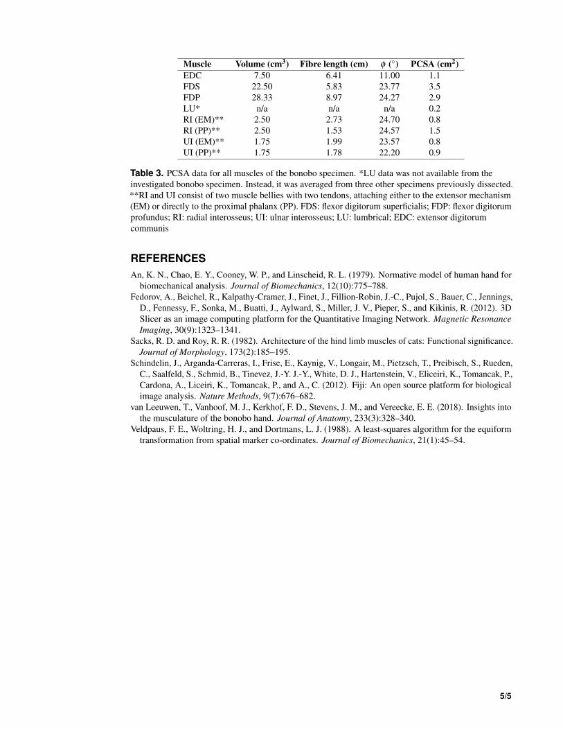
Muscle Volume (cm3) Fibre length (cm) φ (◦) PCSA (cm2)EDC 7.50 6.41 11.00 1.1FDS 22.50 5.83 23.77 3.5FDP 28.33 8.97 24.27 2.9LU* n/a n/a n/a 0.2RI (EM)** 2.50 2.73 24.70 0.8RI (PP)** 2.50 1.53 24.57 1.5UI (EM)** 1.75 1.99 23.57 0.8UI (PP)** 1.75 1.78 22.20 0.9

Table 3. PCSA data for all muscles of the bonobo specimen. *LU data was not available from theinvestigated bonobo specimen. Instead, it was averaged from three other specimens previously dissected.**RI and UI consist of two muscle bellies with two tendons, attaching either to the extensor mechanism(EM) or directly to the proximal phalanx (PP). FDS: flexor digitorum superficialis; FDP: flexor digitorumprofundus; RI: radial interosseus; UI: ulnar interosseus; LU: lumbrical; EDC: extensor digitorumcommunis

REFERENCESAn, K. N., Chao, E. Y., Cooney, W. P., and Linscheid, R. L. (1979). Normative model of human hand for

biomechanical analysis. Journal of Biomechanics, 12(10):775–788.Fedorov, A., Beichel, R., Kalpathy-Cramer, J., Finet, J., Fillion-Robin, J.-C., Pujol, S., Bauer, C., Jennings,

D., Fennessy, F., Sonka, M., Buatti, J., Aylward, S., Miller, J. V., Pieper, S., and Kikinis, R. (2012). 3DSlicer as an image computing platform for the Quantitative Imaging Network. Magnetic ResonanceImaging, 30(9):1323–1341.

Sacks, R. D. and Roy, R. R. (1982). Architecture of the hind limb muscles of cats: Functional significance.Journal of Morphology, 173(2):185–195.

Schindelin, J., Arganda-Carreras, I., Frise, E., Kaynig, V., Longair, M., Pietzsch, T., Preibisch, S., Rueden,C., Saalfeld, S., Schmid, B., Tinevez, J.-Y. J.-Y., White, D. J., Hartenstein, V., Eliceiri, K., Tomancak, P.,Cardona, A., Liceiri, K., Tomancak, P., and A., C. (2012). Fiji: An open source platform for biologicalimage analysis. Nature Methods, 9(7):676–682.

van Leeuwen, T., Vanhoof, M. J., Kerkhof, F. D., Stevens, J. M., and Vereecke, E. E. (2018). Insights intothe musculature of the bonobo hand. Journal of Anatomy, 233(3):328–340.

Veldpaus, F. E., Woltring, H. J., and Dortmans, L. J. (1988). A least-squares algorithm for the equiformtransformation from spatial marker co-ordinates. Journal of Biomechanics, 21(1):45–54.

5/5