Strong displacement discontinuities and Lagrange ... · Strong displacement discontinuities and Lagrange multipliers: ... displacement discontinuity is presented. ... Strong displacement

www.lajss.orgLatin American Journal of Solids and Structures 2 (2005) 77–88

Strong displacement discontinuities and Lagrange multipliers: finitedisplacement formulation in the analysis of fracture problems

P. M. A. Areias, J. M. A. Cesar de Saa,∗ and C. A. Conceicao Antonio

IDMEC – Instituto de Engenharia MecanicaFEUP – Faculdade de Engenharia da Universidade do Porto, Portugal

Abstract

A finite displacement formulation of a quadrilateral element containing an embeddeddisplacement discontinuity is presented. Lagrange multipliers are adopted to ensure thecrack closure before initiation. Six additional degrees of freedom in each element allow therepresentation of the various states of the crack. The discretized equilibrium equations areexposed, along with the corresponding exact linearization. Two examples illustrate both therobustness and the accuracy of the algorithms.

Keywords: Embedded discontinuities, fracture, finite displacement, Lagrangre multipliers.

1 Introduction

The modern finite element analysis of crack initiation and propagation in solids can be carriedout through the use of embedded strong discontinuities.

Studies regarding embedded strong discontinuities were carried out, for example, in ref-erences [2, 5, 6, 8, 9] for small strain situations and in reference [7] for finite strain situationsusing triangular elements. These techniques circumvent the necessity for remeshing and requireless parameters than standard regularized strain softening implementations. However, penaltyparameters are often adopted for closing the crack.

The use of Lagrange multipliers for closing the crack before propagation is clearly an ap-propriate methodology to avoid penalty parameters and therefore reduce the amount of datarequired to accomplish a simulation.

Two important aspects for an efficient implicit finite element analysis of these problems arethe algorithm robustness and the verified rate of convergence of the Newton-Raphson method(which, for conservative systems with Lagrange multipliers, can be classified as Lagrange-Newton). Here, an exact linearization of the discretized equilibrium equations is carried out.

∗ Corresponding author E-mail: [email protected] Received 05 November 2004

From Recent Developments in the Modelling of Rupture in Solids Conference, ed. A. Benallal & S.P.B. Proenca.

78 P. M. A. Areias, J. M. A. Cesar de Sa and C. A. Conceicao Antonio

2 The kinematics of the element

2.1 The element with an embedded displacement discontinuity: notation

For conciseness, the general considerations regarding the presence of a displacement discontinuitycan be consulted elsewhere (see references [2, 9] ).

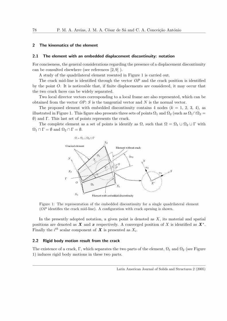
A study of the quadrilateral element resented in Figure 1 is carried out.The crack mid-line is identified through the vector OP and the crack position is identified

by the point O. It is noticeable that, if finite displacements are considered, it may occur thatthe two crack faces can be widely separated.

Two local director vectors corresponding to a local frame are also represented, which can beobtained from the vector OP: S is the tangential vector and N is the normal vector.

The proposed element with embedded discontinuity contains 4 nodes (k = 1, 2, 3, 4), asillustrated in Figure 1. This figure also presents three sets of points Ω1 and Ω2 (such as Ω1∩Ω2 =∅) and Γ. This last set of points represents the crack.

The complete element as a set of points is identify as Ω, such that Ω = Ω1 ∪ Ω2 ∪ Γ withΩ1 ∩ Γ = ∅ and Ω2 ∩ Γ = ∅.

Figure 1: The representation of the embedded discontinuity for a single quadrilateral element(OP identifies the crack mid-line). A configuration with crack opening is shown.

In the presently adopted notation, a given point is denoted as X, its material and spatialpositions are denoted as X and x respectively. A converged position of X is identified as X ∗.Finally the ith scalar component of X is presented as Xi.

2.2 Rigid body motion result from the crack

The existence of a crack, Γ, which separates the two parts of the element, Ω1 and Ω2 (see Figure1) induces rigid body motions in these two parts.

Latin American Journal of Solids and Structures 2 (2005)

Strong displacement discontinuities and Lagrange multipliers 79

The rigid body motion displacements field of the two separated elements parts (Ω1 and Ω2

in 1) should be included into the original displacement field corresponding to the non-crackedelement.

If the converge coordinates X ∗ of an arbitrary point X ∈ Ω1 ∪ Ω2 are considered, the dis-placement vector of this point due to the crack induced rigid body motion can be approximatelycalculated as:

u (X∗, r) =[

S∗1 N∗1

S∗2 N∗2

]

[cosα3 −r senα3

r senα3 cosα3

] [O∗X∗.S∗

O∗X∗.N∗

]−

[O∗X∗.S∗

O∗X∗.N∗

]

︸︷︷︸rotation

+

+[

r α1

r α2

]

︸︷︷︸displacement

(1)

where α1, α2, α3 are internal variables and r is a number belonging to the set −1, 1.This definition presents the use of three internal variables αi. The variable α3 represents

the crack face rotation. The variables α1 and α2 represent the local displacements of the uppercrack face at the point O (see Figure 1).

These internal variables are additive, in contrast with the result u.A representation of the scalar components of u can be carried out as u1 = f1 (α1, α2, α3)

and u2 = f2 (α1, α2, α3). The functions f1 e f2 are introduced to allow the representation ofthe displacement jump at Γ.

The motivation of the use of the parameter r ∈ −1, 1 in equation (1) is to identify the setof points to which X belongs. For X ∈ Ω1 then r = 1 and for X ∈ Ω2 then r = −1.

For the analysis of the crack opening, it is necessary to rewrite a relation analogous to (1)in local coordinates and valid for X ∈ Γ.

In the local frame S, N the scalar components of the local relative displacements at Γ canbe denoted as w1 and w2. To ensure that no penetration takes place between Ω1 and Ω2 it isnecessary to verify w1 ∈ < and w2 ∈ <+

0 .The global displacement w corresponding to the local coordinates w1 and w2 can be written

as:

w =[

S∗1 N∗1

S∗2 N∗2

] [w1

w2

]in Γ (2)

If the crack is closed, both u and w should be null vectors, a fact that can be achieved byensuring that αi = 0, i = 1, 2, 3.

The approximation (1) can be specified for a given node k, according to:



uk = u

X∗

k ,(X∗

k −O) .N∣∣(X∗k −O

).N

∣∣︸︷︷︸

r

(3)

in Ω1 ∪ Ω2.A notation for the scalar components of uk can be carried out as: uk1 = fk1 (α1, α2, α3)

and uk2 = fk2 (α1, α2, α3).With the introduction of the particular case (3), it is possible to define the contribution of

the crack to the rigid body displacement field as:

u = Hkuk (4)

in which Hk are the standard isoparametric shape functions for the quadrilateral.The total displacement field, u , can then be determined as the sum of the regular displace-

ment (which is identified with a hat, u) and the jump:

u = u︸︷︷︸regular

− u︸︷︷︸jump

(5)

The regular displacement field corresponds to the displacement that occurs in the elementrepresented in grey in Figure 1, but without considering the discontinuity.

2.3 The deformation gradient and the spatial velocity gradient

With the definition of the displacement increment field, and hence of the displacement field, thederived quantities follow using classical relations from continuum mechanics (see the presentationgiven by Haupt [4]).

The discretized form of the deformation gradient can be written as:

F = F − F + I + δΓw ⊗N in Ω (6)

The term δΓ in equation (6) represents the Dirac delta function defined on the set Γ. Theterms F and F can be evaluated according to its scalar components:

Fij =∂Hk

∂Xj(Xki + uki) in Ω1 ∪ Ω2 (7)

andFij =

∂Hk

∂Xj(Xki + uki) in Ω1 ∪ Ω2 (8)

The spatial velocity gradient (in Ω) can be denoted as L, and its scalar components are:



Lij =∂Hk

∂xjuki + gijpαp + δΓ ˙wiNkF

−1kj in Ω (9)

In equation (9), the quantity

gijp = −∂Hr

∂xj

∂fr

∂αp(10)

was introduced.

2.4 Existence of the displacement discontinuity

If the displacement discontinuity does not exist, which occurs when a fracture criterion is notsatisfied, then αi = 0. This is imposed through the introduction of a function h of the crackstate which is defined as:

h =

0 crack closed

1 crack opened

If h= 0 then αi = 0 for i = 1, 2, 3. A suitable method for imposing the constraints αi = 0 is theLagrange multiplier method, which is here adopted.

3 Equilibrium equations and related discretized forms

Let V0 represent the material integration volume corresponding to the domain Ω1 ∪ Ω2 and v0

represent the spatial integration volume corresponding to the same domain. The element isdefined as Ω.

The crack zone itself is represented by the material integration line l0. A given point X ∈Ω1 ∪ Ω2 is represented by its material coordinates X and spatial coordinates x=X+u .

As u(X ) and u(X ) are two independent fields, they can be used to introduce kinematicallyadmissible virtual displacements δ u and δ u to project the equilibrium equations and obtain aweak form.

The existence of a volume force field represented by its material vector b (X) is assumed.If τ (F ) represents the Kirchhoff stress tensor, then the weak form of equilibrium can be

exposed as:∫

V oτ (F ) : ∇x δu dV o +

∫

loδw . t dlo =

∫

V ob . δu dV o in Ω (11)

This project form is very similar to the standard projected form for a non-cracked element(with the noticeable exception of the crack term).

The condition for the non-existence of the crack is introduced imposing ui = 0 for h = 0.Additionally, the condition for crack closure should be introduced for h = 1. If Lagrangemultipliers λ are introduced then:



∫

V oτ (F ) : ∇xδu dV o +

∫

loδw . t dlo + δ [λ ((1− h) α + hλ)] =

∫

V ob . δu dV o (12)

For the application of the Newton-Raphson method, the first variations of equation (12) arerequired.

4 Particular constitutive relations for the discrete crack

4.1 Fracture criterion

If the crack has not initiated yet, which occurs for the indicator h = 0, the following criterionfor the crack initiation is adopted for a given element:

^τ 1 ≥ τ1c (13)

where τ1c is the maximum allowable positive Kirchhoff principal stress and τ1c is the followingquantity:

^τ 1 =

1V o

∫

V omax (0, τ1) dV o (14)

with τ1 being the maximum principal Kirchhoff stress.The definition of h is carried out using the maximum value of τ1c during the deformation

history:

h = H

max︸︷︷︸

history

(^τ 1

)− τ1c

(15)

The function H in definition (15) is the unit step function. The calculation of the naturalcoordinates ξQ of a point Q located on the crack is carried out using the following relation whereξX represent the natural coordinates of a point X ∈ Ω1 ∪ Ω2:

ξQ =

∫V o max (0, τ1) ξX dV o

V o^τ 1

(16)

The calculation of the material coordinates of the normal vector, N , is accomplish accordingto:

N =

∫V o max (0, τ1) N1 dV o

V o^τ 1

(17)

where N 1 is the second Piola-Kirchhoff stress principal direction.



4.2 Interface compliance

The calculate t as a function of w , the local spatial coordinates of t in the frame s,n areintroduced:

t1 = t.s (18a)

t2 = t.n (18b)

Introducing an internal kinematic variable, k, the following local constitutive law is assumedfor t1 and t2:

t1t2

=

dint w1

[Ξ (k) H (w2) + ρH (−w2)] w2

(19)

where Ξ (k) is the following function of k:

Ξ (k) =τ1c

kexp

(− τ1c

Gfk

)(20)

and ρ is a penalty parameter.The value of ρ is taken as the absolute value of the interface compliance before initiation:

ρ =τ21c

Gf= − lim

w2→0+

∂t2∂w2

(21)

In equation (20) the term Gf represents the fracture energy, the term k is calculated usingthe historical evaluation of w2:

k = maxhistory

[max (0, w2)] (22)

The property dint in equation (19) is the shear stiffness of the crack. A constant value ofdint is here adopted, but distinct strategies are possible (see reference [9]).

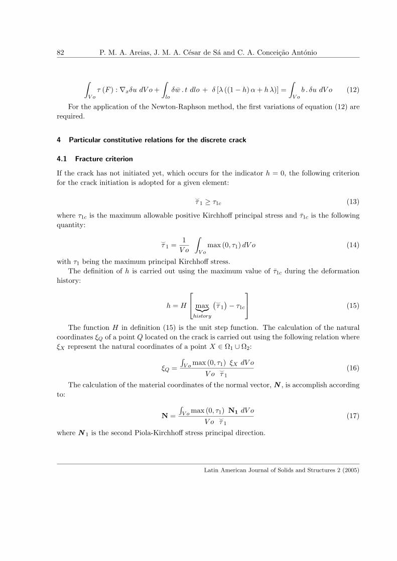
5 Numerical integration

For the domain Ω1 ∪ Ω2, a standard Gaussian quadrature is adopted. For the crack, a nodalintegration rule is employed. Due to the definition of the crack position, both Ω1 and Ω2 containat least one Gauss point.

The integration points are presented in Figure 2.



Figure 2: The integration points in the crack and in the quadrilateral.

6 Numerical examples

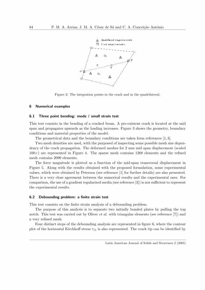
6.1 Three point bending: mode I small strain test

This test consists in the bending of a cracked beam. A pre-existent crack is located at the midspan and propagates upwards as the loading increases. Figure 3 shows the geometry, boundaryconditions and material properties of the model.

The geometrical data and the boundary conditions are taken form references [1, 3].Two mesh densities are used, with the purposed of inspecting some possible mesh size depen-

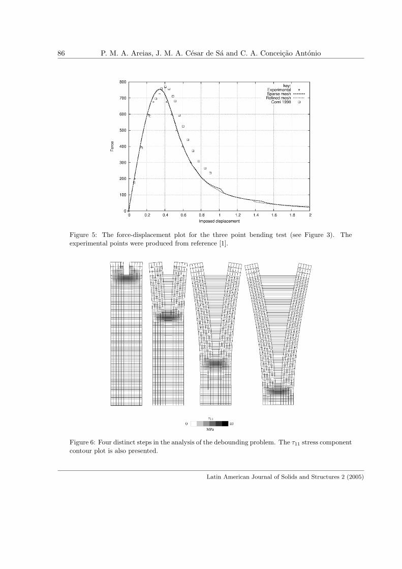
dency of the crack propagation. The deformed meshes for 2 mm mid span displacement (scaled100×) are represented in Figure 4. The sparse mesh contains 1268 elements and the refinedmesh contains 2099 elements.

The force magnitude is plotted as a function of the mid-span transversal displacement inFigure 5. Along with the results obtained with the proposed formulation, some experimentalvalues, which were obtained by Peterson (see reference [1] for further details) are also presented.There is a very close agreement between the numerical results and the experimental ones. Forcomparison, the use of a gradient regularized media (see reference [3]) is not sufficient to representthe experimental results.

6.2 Debounding problem: a finite strain test

This test consists on the finite strain analysis of a debounding problem.The purpose of this analysis is to separate two initially bonded plates by pulling the top

notch. This test was carried out by Oliver et al. with triangular elements (see reference [7]) anda very refined mesh.

Four distinct steps of the debounding analysis are represented in figure 6, where the contourplot of the horizontal Kirchhoff stress τ11 is also represented. The crack tip can be identified by



Figure 3: Three point bending of a cracked beam (all dimensions are in mm).

Figure 4: The deformed meshes (with a scale factor of 100) corresponding to two distinct meshdensities.



Figure 5: The force-displacement plot for the three point bending test (see Figure 3). Theexperimental points were produced from reference [1].

Figure 6: Four distinct steps in the analysis of the debounding problem. The τ11 stress componentcontour plot is also presented.



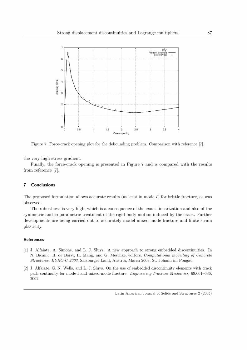
Figure 7: Force-crack opening plot for the debounding problem. Comparison with reference [7].

the very high stress gradient.Finally, the force-crack opening is presented in Figure 7 and is compared with the results

from reference [7].

7 Conclusions

The proposed formulation allows accurate results (at least in mode I) for brittle fracture, as wasobserved.

The robustness is very high, which is a consequence of the exact linearization and also of thesymmetric and isoparametric treatment of the rigid body motion induced by the crack. Furtherdevelopments are being carried out to accurately model mixed mode fracture and finite strainplasticity.

References

[1] J. Alfaiate, A. Simone, and L. J. Sluys. A new approach to strong embedded discontinuities. InN. Bicanic, R. de Borst, H. Mang, and G. Meschke, editors, Computational modelling of ConcreteStructures, EURO-C 2003, Salzburger Land, Austria, March 2003. St. Johann im Pongau.

[2] J. Alfaiate, G. N. Wells, and L. J. Sluys. On the use of embedded discontinuity elements with crackpath continuity for mode-I and mixed-mode fracture. Engineering Fracture Mechanics, 69:661–686,2002.



[3] Comi and L. Driemeier. Material Instabilities in Solids, chapter 26. John Wiley and Sons, 1998.

[4] P. Haupt. Continuum Mechanics and Theory of Materials, second edition. Springer-Verlag, 2002.

[5] M. Jirasek and T. Zimmermann. Embedded crack model. I: Basic formulation. International Journalfor Numerical Methods in Engineering, 50:1269–1290, 2001.

[6] M. Jirasek and T. Zimmermann. Embedded crack model. II: Combination with smeared cracks.International Journal for Numerical Methods in Engineering, 50:1291–1305, 2001.

[7] J. Oliver, A. Huespe, D. Pulido, and E. Samaniego. On strong discontinuity approach in finitedeformation settings. In Monograph CIMNE 62, International Center for Numerical Methods inEngineering, Barcelona, Spain,, October 2001.

[8] L. J. Sluys and A. H. Berends. Discontinuous failure analysis for mode-I and mode-II localizationproblems. International Journal of Solids and Structure, 35:4257–4274, 1998.

[9] G. N. Wells and L. J. Sluys. A new method for modelling cohesive cracks using finite elements.International Journal for Numerical Methods in Engineering, 50:2667–2682, 2001.


Strong displacement discontinuities and Lagrange ... · Strong displacement discontinuities and Lagrange multipliers: ... displacement discontinuity is presented. ... Strong displacement

Documents