HORRY COUNTY Stormwater Management Design Manual SEPTEMBER 2000

Welcome message from author
This document is posted to help you gain knowledge. Please leave a comment to let me know what you think about it! Share it to your friends and learn new things together.
Transcript

HORRY COUNTY
Stormwater Management Design Manual
SEPTEMBER 2000
HORRY COUNTY STORMWATER MANAGEMENT DESIGN MANUAL
Horry County Manual
Table of Contents Chapter 1 ........................................................................................................Introduction Chapter 2 ........................................................................................................... Hydrology Chapter 3 ................................................................................... Storm Drainage Systems Chapter 4 ..............................................................................................Design of Culverts Chapter 5 ........................................................................................Open Channel Design Chapter 6 ................................................................................................Storage Facilities Chapter 7 .................................................... Water Quality Best Management Practices Chapter 8 ................................................................................ Example Stormwater Plan


HORRY COUNTY STORMWATER MANAGEMENT DESIGN MANUAL
Horry County Manual
HORRY COUNTY STORMWATER MANAGEMENT DESIGN MANUAL
Horry County Manual
Acknowledgments The authors would like to thank the members of the Stormwater Technical Review Committee for their participation in the project and assistance in the preparation of this document. Members of the committee are as follows: Robert Castles Castles Consulting Engineers, Inc. Bill Gobbel J. William Gobbel & Associates, Inc. Barry Greene Hardwick & Associates Tim Kirby DDC Engineers, Inc. Mike Redmon Engineering & Technical Services, Inc. Jon Taylor ASI Consulting Engineers & Planners Robert Wilfong Kimley-Horn & Associates The authors would also like to acknowledge the additional local design professionals who made significant contributions to the contents of this document. The firm providing the Example Stormwater Plan in Chapter 8 is: Braxton Lewis A B Consulting Engineers, Inc. The authors would also like to thank the members of the Horry County Engineering Department for all of their support in providing local data and information for this document. Special appreciation goes to: Steven Gosnell Director of Infrastructure and Regulation Tom Garigen Deputy County Engineer The authors would also like to acknowledge the members of the Horry County Council for commissioning and undertaking this Stormwater Management Design Manual. Members of the Council are as follows: Chad C. Prosser Chairman Marvin D. Heyd District 6 Ray E. Skidmore, Jr. District 1 James R. Frazier District 7 John C. Kost District 2 Elizabeth D. Gilland District 8 Ray Brown District 3 Ulysses Dewitt District 9 Chandler Brigham District 4 Johnny M. Shelley District 10 Terry B. Cooper District 5 Janice G. Jordan District 11


HORRY COUNTY STORMWATER MANAGEMENT DESIGN MANUAL
Horry County Manual
INTRODUCTION 1
Horry County Manual 1-1
CHAPTER
Chapter Table of Contents 1.1 Introduction...................................................................................................... 1-2
1.1.1 Purpose ................................................................................................... 1-2 1.1.2 Contents .................................................................................................. 1-3 1.1.3 Planning Concepts .................................................................................. 1-3 1.1.4 OCRM Coordination .............................................................................. 1-4 1.1.5 Downstream Analysis............................................................................. 1-4 1.1.6 Easement Requirements ......................................................................... 1-5 1.1.7 As-Built Plan Requirements ................................................................... 1-6 1.1.8 Limitations of Manual ............................................................................ 1-7 1.1.9 Updating Manual .................................................................................... 1-7 1.1.10 Use of Computer Models for Design..................................................... 1-7
1.1.10.1 Hydrology Software ................................................................. 1-9 1.1.10.2 Hydraulics Software............................................................... 1-11 1.1.10.3 Water Quality Software.......................................................... 1-14

1-2 Horry County Manual
This Page Intentionally Left Blank 1.1 Introduction 1.1.1 Purpose

Horry County Manual 1-3
This manual has been developed to assist in the design and evaluation of stormwater management facilities within the Horry County, South Carolina area. It provides engineering design guidance to:
• local agencies responsible for implementing the Horry County Stormwater Management Program,
• engineers responsible for the design of stormwater management structures, • developers involved in site planning and design, • others involved in stormwater management at various levels who may find the manual
useful as a technical reference to define and illustrate engineering design techniques. Application of the procedures and criteria presented in this manual should contribute toward the effective and economical mitigation and solution of local drainage and flooding problems. Application of the procedures should also contribute to more uniform design and analysis of stormwater management facilities throughout Horry County. Engineering design methods other than those included in this manual can be used if approved by the County Engineering Department. Complete documentation of these methods may be required for approval. 1.1.2 Contents The manual presents technical and engineering procedures and criteria needed to comply with the Horry County Stormwater Management And Sediment Control Ordinance. Following are the chapters included in the manual: Chapter 1 Introduction Chapter 2 Hydrology Chapter 3 Storm Drainage Systems Chapter 4 Design of Culverts Chapter 5 Open Channel Hydraulics Chapter 6 Storage Facilities Chapter 7 Water Quality Best Management Practices Chapter 8 Example Stormwater Plan Each chapter contains the equations, charts, and nomographs needed to design specific stormwater management facilities. Example problems are used to illustrate the use of the procedures. Where appropriate desktop computer procedures are developed for design applications. 1.1.3 Planning Concepts In addition to the engineering procedures and criteria necessary for stormwater management, there are many planning concepts that should be considered. Drainage planning involves the interaction of many elements within the planning process. Many advantages accrue to developers, residents, and local governmental units when drainage planning is undertaken at an early stage in the planning process. Advantages may include lower cost drainage facilities, decreased flooding and maintenance problems, and facilities that provide more benefits. Thus the planner and drainage engineer should work in close cooperation to achieve maximum benefits for each dollar invested. Good drainage planning is a complex process. Land use planning and location of developments should be closely coordinated with drainage planning to prevent drainage problems. Early in the planning and development process, consideration should be given to major flood events, local

1-4 Horry County Manual
drainage from small areas, and environmental consequences of proposed actions. As an example when planning a new subdivision, various drainage configurations should be considered before decisions are made on block layout and street location. Sensitive environmental areas should be identified and integrated into the final plan. It is perhaps at this point in the development process where the greatest impact can be made on the cost of proposed drainage facilities. Also, the planning and design of drainage facilities and associated land use planning should consider flood hazard areas at an early stage to avoid unnecessary complications. There are also many secondary benefits received from good drainage planning:
• reduced street maintenance costs, • reduced street construction costs, • improved movement of traffic, • improved public health, • lower cost open space, • lower cost park areas and more recreational opportunities, • development of otherwise undevelopable land, • opportunities for lower building costs, • reduced County administrative costs, and • reduced maintenance costs of drainage facilities.
Design engineers are encouraged to work with the Horry County Engineering Department as early in the planning and development process as possible, when the maximum number of drainage alternatives are possible. Much time and expense can often be avoided with good cooperation between the engineer/developer and the County. 1.1.4 OCRM Coordination The South Carolina Office of Ocean and Coastal Resource Management (OCRM) is currently involved in the review of development plans for compliance with water quality and other stormwater management regulations. As Horry County gains experience in implementing the Horry County Stormwater Management And Sediment Control Ordinance and the design procedures contained in this manual, it is anticipated that more responsibility related to stormwater management will be transferred to the County and less review and approval will be done through OCRM. Until this transfer occurs, OCRM will also have review and approval responsibility of stormwater management plans for new developments. OCRM has published technical documents that should be consulted, in addition to this manual, when planning and designing stormwater management facilities, erosion and sediment control, and water quality best management practices. These include:
• Policies and Procedures of the South Carolina Coastal Management Program, Updated July 1995.
• Your Guide to Important Coastal Programs, August 2, 1993. • South Carolina Stormwater Management and Sediment Control Handbook for Land
Disturbance Activities, February 1997. 1.1.5 Downstream Analysis Performing a hydrologic-hydraulic study downstream from stormwater management facilities and urban developments is an important part of urban stormwater management. Often design conditions
Horry County Manual 1-5
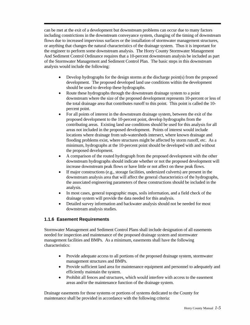
can be met at the exit of a development but downstream problems can occur due to many factors including constrictions in the downstream conveyance system, changing of the timing of downstream flows due to increased impervious surfaces or the installation of stormwater management structures, or anything that changes the natural characteristics of the drainage system. Thus it is important for the engineer to perform some downstream analysis. The Horry County Stormwater Management And Sediment Control Ordinance requires that a 10-percent downstream analysis be included as part of the Stormwater Management and Sediment Control Plan. The basic steps in this downstream analysis would include the following:
• Develop hydrographs for the design storms at the discharge point(s) from the proposed development. The proposed developed land use conditions within the development should be used to develop these hydrographs.
• Route these hydrographs through the downstream drainage system to a point downstream where the size of the proposed development represents 10-percent or less of the total drainage area that contributes runoff to this point. This point is called the 10-percent point.
• For all points of interest in the downstream drainage system, between the exit of the proposed development to the 10-percent point, develop hydrographs from the contributing areas. Existing land use conditions should be used for this analysis for all areas not included in the proposed development. Points of interest would include locations where drainage from sub-watersheds intersect, where known drainage and flooding problems exist, where structures might be affected by storm runoff, etc. As a minimum, hydrographs at the 10-percent point should be developed with and without the proposed development.
• A comparison of the routed hydrograph from the proposed development with the other downstream hydrographs should indicate whether or not the proposed development will increase downstream peak flows or have little or not affect on these peak flows.
• If major constructions (e.g., storage facilities, undersized culverts) are present in the downstream analysis area that will affect the general characteristics of the hydrographs, the associated engineering parameters of these constructions should be included in the analysis.
• In most cases, general topographic maps, soils information, and a field check of the drainage system will provide the data needed for this analysis.
• Detailed survey information and backwater analysis should not be needed for most downstream analysis studies.
1.1.6 Easement Requirements Stormwater Management and Sediment Control Plans shall include designation of all easements needed for inspection and maintenance of the proposed drainage system and stormwater management facilities and BMPs. As a minimum, easements shall have the following characteristics:
• Provide adequate access to all portions of the proposed drainage system, stormwater management structures and BMPs.
• Provide sufficient land area for maintenance equipment and personnel to adequately and efficiently maintain the system.
• Prohibit all fences and structures, which would interfere with access to the easement areas and/or the maintenance function of the drainage system.
Drainage easements for those systems or portions of systems dedicated to the County for maintenance shall be provided in accordance with the following criteria:
1-6 Horry County Manual
1) The width of piped drainage easements shall be determined using the following
equation: Easement Width = [Pipe Depth (in feet) x 4] + [Pipe Diameter (in feet)]
The calculated piped drainage easement shall always be rounded up to the next higher 5-foot increment. Also, the minimum width for any piped drainage easement shall be twenty (20) feet.
2) Minimum pipe size acceptable for County maintenance shall be fifteen (15) inches. 3) For multiple pipes, box culverts or multiple box culverts, the easement width shall be
the outside diameter or width of the system plus ten (10) feet on one side and fifteen (15) feet on the other side of the system, but the minimum total shall not be less than thirty (30) feet.
4) For open channel easements, the following widths shall apply: a) When the top width of the channel is equal to or less than fifteen (15) feet,
the following equation shall be used: Easement Width = (25-foot offset on one side) + (Channel Top Width) + (5-foot offset on the other side)
b) When the top width of the channel exceeds fifteen (15) feet, the following equation shall be used:
Easement Width = (25-foot offset on one side) + (Channel Top Width) + (25-foot offset on the other side)
5) For minor swales along lot lines where the side slopes are equal to or flatter than 3:1 and the depth does not exceed fifteen (15) inches, a drainage easement not less than twenty (20) feet in width shall be provided.
6) Open ditches within street rights-of-way or along roadways shall have side slopes no steeper than 3:1. Open ditches along rear lot lines shall have side slopes no steeper than 1:1.
7) All ditches deeper than thirty-six (36) inches shall be piped. 8) For detention basins and other stormwater management facilities, a 12-foot drainage
easement shall be provided around the facility and beyond the 25-year design storm water surface elevation.
1.1.7 As-Built Plan Requirements Upon completing the installation of the stormwater management facilities included in the Stormwater Management and Sediment Control Plan, an "as-built" plan signed and sealed by a professional registered in South Carolina shall be submitted to the Horry County Engineering Department for review and approval. The registered professional shall state that:
• The facilities have been constructed as shown on the "as-built" plan, and • The facilities meet the approved Stormwater Management and Sediment Control Plan
and specifications or achieve the function for which they were designed. Also, the minimum information to be provided on the "as-built" plans shall include the following:
1) Boundary, phase and lot lines. 2) Lot numbers and street names. 3) Easements. 4) Road locations with centerline stationing and curve data. 5) Road centerline elevations at 100-foot intervals. 6) Drainage structures with elevations. 7) Drainage pipes with size, material, length, slope and invert elevations. 8) Ponds or lakes with average bottom and water surface elevations, and any control

Horry County Manual 1-7
structures shall be shown in detail. 9) Drainage ditches and swales, with elevations at 100-foot intervals. 10) Water and sewer as-built information as required by the appropriate utility company.
Additional information may be required by the County Engineer as deemed necessary to adequately document the “As-Built” condition of the road and drainage systems. 1.1.8 Limitations of Manual This manual provides a compilation of readily available literature relevant to stormwater management activities within Horry County. Although it is intended to establish uniform design practices, it neither replaces the need for engineering judgment nor precludes the use of information not presented. Since the material presented was obtained from numerous publications, which have not been duplicated in their entirety, the user is encouraged to obtain original or additional reference material, as appropriate. Acquiring additional information may be necessary for complex design situations. References, including references to available computer programs, are included at the end of each chapter. 1.1.9 Updating Manual This manual will be updated and revised, as necessary, to reflect up-to-date practices and information applicable to Horry County. Registered manual users who provide a current address will automatically be sent changes as they are produced. Current manuals can be obtained from the Horry County Engineering Department. 1.1.10 Use of Computer Models for Design Given the complexity of urban stormwater design and analysis, the use of computer models is common in urban drainage design. There are numerous models available to the engineer from both public and private sources. The purpose of the following discussion is not to limit the computer models that can be used in Horry County but instead to present some of the more commonly used models. Other models may be used for design and analysis if approved by the Horry County Engineering Department. Please contact the Engineering Department if you are not sure whether or not a particular model is acceptable in Horry County. There is no one engineering software that addresses all hydrologic, hydraulic and water quality situations. Design needs and troubleshooting for watershed and stormwater management occur on several different scales and can be either system-wide (i.e., watershed) or localized. System-wide issues can occur on both large and small drainage systems, but generally require detailed, and often expensive, system-wide models and or design tools. The program(s) chosen to address these issues should handle both major and minor drainage systems. Localized issues also exist on both major and minor drainage systems, but unlike system-wide problems, flood and water quality solution alternatives can usually be developed quickly and cheaply using simpler engineering methods and design tools. The goal of this discussion is to present a number of hydrology, hydraulics and water quality modeling packages and design tools commonly used in the United States to solve stormwater related issues. For purposes of this discussion, major drainage systems are the watershed receiving waters. Typically this is a FEMA-regulated natural stream or EPA-regulated lake or reservoir to which stormwater runoff ultimately drains. Minor drainage systems are the smaller natural and man-made systems that drain to the more major streams. Minor drainage systems have both closed and open-channel components and can include, but are not limited to, neighborhood storm sewers, culverts, ditches, and tributaries.

1-8 Horry County Manual
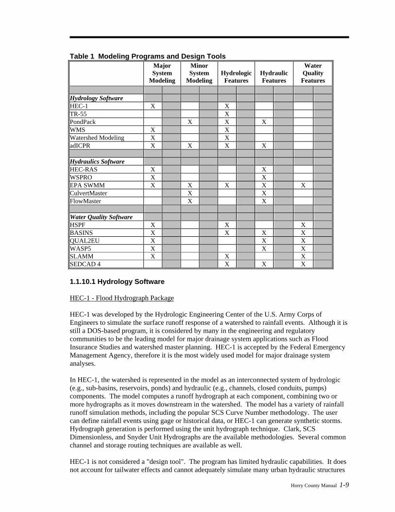
Table 1 lists the programs that are included in the following discussion. The programs were examined for their applicability to both system-wide and localized issues, the methodologies used for computations, and ease-of-use. They are categorized in accordance with their primary application (i.e., the application for which they were originally developed), hydrology, hydraulics or water quality, although several programs can be used for more than one application. Hydrology programs calculate the quantity of runoff from a watershed and drainage basin. The primary purpose of such a program is to determine peak flows or generate runoff hydrographs. The basic duties of a hydraulics program, depending upon the application, would be to calculate flood elevations, compute flows through culverts and bridges, perform stormwater pipe network calculations or allow the design of channels and pipes. Water quality programs determine pollutant loads or concentrations in runoff or receiving waters. Most of the programs listed have capabilities beyond those outlined above. A brief description of program capabilities and methodologies are presented in a short discussion of each program that follows Table 1.
Horry County Manual 1-9
Table 1 Modeling Programs and Design Tools
Major System
Modeling
Minor System
Modeling
Hydrologic
Features
Hydraulic Features
Water Quality
Features
Hydrology Software HEC-1 X X TR-55 X PondPack X X X WMS X X Watershed Modeling X X adICPR X X X X
Hydraulics Software HEC-RAS X X WSPRO X X EPA SWMM X X X X X CulvertMaster X X FlowMaster X X
Water Quality Software HSPF X X X BASINS X X X X QUAL2EU X X X WASP5 X X X SLAMM X X X SEDCAD 4 X X X 1.1.10.1 Hydrology Software HEC-1 - Flood Hydrograph Package HEC-1 was developed by the Hydrologic Engineering Center of the U.S. Army Corps of Engineers to simulate the surface runoff response of a watershed to rainfall events. Although it is still a DOS-based program, it is considered by many in the engineering and regulatory communities to be the leading model for major drainage system applications such as Flood Insurance Studies and watershed master planning. HEC-1 is accepted by the Federal Emergency Management Agency, therefore it is the most widely used model for major drainage system analyses. In HEC-1, the watershed is represented in the model as an interconnected system of hydrologic (e.g., sub-basins, reservoirs, ponds) and hydraulic (e.g., channels, closed conduits, pumps) components. The model computes a runoff hydrograph at each component, combining two or more hydrographs as it moves downstream in the watershed. The model has a variety of rainfall runoff simulation methods, including the popular SCS Curve Number methodology. The user can define rainfall events using gage or historical data, or HEC-1 can generate synthetic storms. Hydrograph generation is performed using the unit hydrograph technique. Clark, SCS Dimensionless, and Snyder Unit Hydrographs are the available methodologies. Several common channel and storage routing techniques are available as well. HEC-1 is not considered a "design tool". The program has limited hydraulic capabilities. It does not account for tailwater effects and cannot adequately simulate many urban hydraulic structures

1-10 Horry County Manual
such as pipe networks, culverts and multi-stage detention pond outlet structures. However, there are other hydrologic applications developed within HEC-1 that have been utilized with much success. Multiplan-multiflood analyses allow the user to simulate a number of flood events for different watershed situations (or plans). The dam safety option enables the user to analyze the impact of dam overtopping or structural failure on downstream areas. Flood damage analyses assess the economic impact of flood damage. Because it is not a Windows-based program, HEC-1 does not have easy to use input and output report generation and graphical capabilities, and therefore is generally not considered a user-friendly program. However, because of its wide acceptance, several software development companies have incorporated the source code into enhanced "shells" to provide a user-friendly interface and graphical input and output capabilities. Examples of these programs include Graphical HEC-1 developed by Haested Methods and WMS developed by the Environmental Modeling Research Laboratory. The Corps of Engineers has developed a user-friendly, Windows-based Hydrologic Modeling System (HEC-HMS) intended to replace the DOS-based HEC-1 model. The new program has all the components of HEC-1, with more user-friendly input and output processors and graphical capabilities. HEC-1 files can be imported into HEC-HMS. Version 2 of this model has been released, however its acceptance and use is limited at this time. While highly anticipated by the engineering community, widespread use of HEC-HMS has been slow to develop, mainly due to the necessity for the Corps of Engineers to further develop, modify and "debug" the early program. FEMA is expected to approve the model after some length of time. TR-55 - Technical Release 55 The TR-55 model is a DOS-based software package used for estimating runoff hydrographs and peak discharges for small urban watersheds. The model was developed by the Soil Conservation Service, and therefore uses SCS methodology to estimate runoff. No other methodology is available in the program. Four 24-hour regional rainfall distributions are available for use. Rainfall durations less than 24-hours cannot be simulated. Using detailed input data entered by the user, the TR-55 model can calculate the area-weighted CN, time of concentration and travel time. Detention pond (i.e., storage) analysis is also available in the TR-55 model, and is intended for initial pond sizing. Final design requires a more detailed analysis. TR-55 is easy-to-use, however because it is DOS-based it does not have the useful editing and graphical capabilities of a Windows-based program. Haestad Methods, Inc., included most of the TR-55 capabilities in its PondPack program. A detailed description of PondPack is included in the following paragraphs. PONDPACK PondPack, by Haestad Methods, Inc., is Windows-based software developed for modeling general hydrology and runoff from site development. The program analyzes pre- and post-developed watershed conditions and sizes detention ponds. It also computes outlet rating-curves with consideration of tailwater effects, accounts for pond infiltration, calculates detention times and analyzes channels. Rainfall options are unlimited. The user can model any duration or distribution, for synthetic or real storm events. Several peak discharge and hydrograph computation methods are available, including SCS, the Rational Method and the Santa Barbara Unit Hydrograph procedure. Infiltration can be considered, and pond and channel routing options are available as well. Like TR-55, PondPack allows the user to calculate hydrologic parameters, such as the time of
Horry County Manual 1-11
concentration, within the program. PondPack has limited, but useful hydraulic features, using Manning's equation to model natural and man-made channels and pipes. A wide variety of detention pond outlet structure configurations can be modeled, including low flow culverts, weirs, riser pipes, and even user-defined structures. WMS - Watershed Modeling System WMS was developed by the Engineer Computer Graphics Laboratory of Brigham Young University. WMS is a Windows-based user interface that provides a link between terrain models and GIS software, with industry standard lumped parameter hydrologic models, including HEC-1, TR-55, TR-20 and others. The hydrologic models can be run from the WMS interface. The link between the spatial terrain data and the hydrologic model(s) gives the user the ability to develop hydrologic data that is typically gathered using manual methods from within the program. For example, when using SCS methodologies, the user can delineate watersheds and sub-basins, determine areas and curve numbers, and calculate the time of concentration within the computer program. Typically, these computations are done manually, and are laborious and time-consuming. WMS attempts to utilize digital spatial data to make these tasks more efficient. Watershed Modeling The Watershed Modeling program was developed to compute runoff and design flood control structures. The program can run inside MicroStation, the computer aided design software developed by Bentley. Like WMS, this feature enables the program to delineate and analyze the drainage area of interest. Area, curve number, landuse and other hydrologic parameters can be computed and/or catalogued for the user, removing much of the manual calculation typically performed by the hydrologic modeler. Watershed Modeling contains a variety of methods to calculate flood hydrographs, including SCS, Snyder and Rational methods. Rainfall can be synthetic or user-defined, with any duration and return period. Rainfall maps for the entire United States are provide to help the user calculate IDF relationships. Several techniques are available for channel and storage routing. The user also has a wide variety of outlet structure options for detention pond analysis and design. adICPR adICPR is a stormwater management analysis and design tool for hydrologic and hydraulic analysis and design. The model is operated by an executive module that transfers control to numerous other routines. There are routines to input and edit data, compute runoff hydrographs and flood route hydrographs through complex pond and conveyance systems. Results can be reviewed and analyzed with a database retrieval system. A variety of tabular and graphical reports can be easily generated for review by the user or for submittal to reviewing agencies. The model addresses the relatively complex problems of interdependent pond systems. Time variable tailwater conditions, flow reversals and looped hydraulic networks are included. The model analyzes an extensive array of hydraulic structures including culverts under all flow regimes. adICPR allows for hydrodynamic channel routing. The adICPR model includes several hydrograph options including the SCS Unit Hydrograph Method, Santa Barbara Urban Hydrograph Method and the Kinematic Overland Flow Methods. 1.1.10.2 Hydraulics Software HEC-RAS - River Analysis System

1-12 Horry County Manual
HEC-RAS is a Windows-based hydraulic model developed by the Corps of Engineers to replace the popular, DOS-based HEC-2 model. HEC-RAS has the ability to import and convert HEC-2 input files and expounds upon the capabilities of HEC-2. Since its introduction several years ago, the user-friendly HEC-RAS has become known as an excellent model for simulation of major systems (i.e., open channel flow) and has become the chief model for calculating floodplain elevations and determining floodway encroachments for Flood Insurance Studies. Like HEC-2, HEC-RAS has been accepted for FIS analysis by the FEMA. However, HEC-RAS is a much easier model to use than HEC-2 as it has an extremely useful interface that provides the immediate capability to view model input and output data in both graphical, tabular, and report formats. HEC-RAS performs one-dimensional analysis for steady flow water surface profiles, using the energy equation. Energy losses are calculated using Manning's equation and contraction and expansion changes. Rapidly varied flow (e.g., hydraulic jumps) is modeled using the momentum equation. The effects of in-stream structures, such as bridges, culverts, weirs and floodplain obstructions and in-stream changes such as levees and channel improvements can be simulated. The model allows the user to define the geometry of the channel or structure to the level of detail required by the application. One popular and useful feature of the HEC-RAS model is the capability to easily facilitate floodway encroachment analysis. Five encroachment methods are available to the user. The Corps of Engineers has stated that future versions of the HEC-RAS model will have components for unsteady flow and sediment transport simulations. In the model's original form, HEC-RAS does not provide a tie to GIS information. However the model was designed with GIS applications in mind and future ties between HEC-RAS and GIS platforms are anticipated. Several software developers have already released enhanced versions of HEC-RAS that provide the capability to import GIS data for channel geometry and export HEC-RAS output for floodplain and floodway delineation. Examples of such software include BOSS RMS, developed by BOSS International and SMS (Surface Water Modeling System), distributed by the Scientific Software Group. WSPRO WSPRO was developed by the USGS to compute water surface profiles for one-dimensional, gradually varied, steady flow. Like HEC-RAS, WSPRO can develop profiles in subcritical, critical and supercritical flow regimes. WSPRO is designated HY-7 in the Federal Highway Administration (FHWA) computer program series and its original objective was analysis and design of bridge openings and embankment configurations. Since then, the model has been expanded to model open channels and culverts. Open channel computations use standard step-backwater techniques. Flow through bridges is simulated using an energy-balancing technique that uses a coefficient of discharge and estimates an effective flow length. Pressure flow under bridges uses orifice-type flow equations developed by the FHWA. Culvert flow is simulated using FHWA techniques for inlet control and energy balance for outlet control. WSPRO is considered a fairly easy-to-use DOS-based model, applicable to water surface profile analysis for highway design, flood insurance studies, and establishing stage-discharge relationships. However, the model in its original form is not Windows based and therefore does not have the useful editing and graphical features found in HEC-RAS. Like HEC-RAS, a third party software developer has designed SMS (Surface Water Modeling Software) to support both pre- and post-processing of WSPRO data.
Horry County Manual 1-13
EPA SWMM - Storm Water Management Model EPA SWMM was developed by the Environmental Protection Agency (EPA) to analyze stormwater quantity and quality problems associated with runoff from urban areas. EPA SWMM has become the model of choice for simulation of minor drainage systems primarily composed of closed conduits. The model can simulate both single-event and continuous events and has the capability to model both wet and dry weather flow. The basic output from SWMM consists of runoff hydrographs, pollutographs, storage volumes and flow stages and depths. SWMM's hydraulic computations are link-node based, and are performed in separate modules, called blocks. The EXTRAN computational block solves complete dynamic flow routing equations to simulate backwater, looped pipe connections, manhole surcharging and pressure flow. It is the most comprehensive model in its capabilities to simulate urban storm flow, which many cities have used successfully for stormwater, sanitary, or combined sewer system modeling. Open channel flow can be simulated using the TRANSPORT block, which solves the kinematic wave equations for natural channel cross-sections. Although evaluated as a hydraulic model, SWMM has both hydrologic and water quality components. Hydrologic processes are simulated using the RUNOFF block, which computes the quantity and quality of runoff from drainage areas and routes the flow to the major sewer system lines. Pollutant transport is simulated in tandem with hydrologic and hydraulic computations and consists of the calculation of pollutant buildup and washoff from land surfaces and pollutant routing, scour and in-conduit suspension in flow conduits and channels. EPA SWMM is a public domain, DOS-based model. For large watersheds with extensive pipe networks, input and output processing can be tedious and confusing. Because of the popularity of the model commercial, third-party enhancements to SWMM have become more common, making the model a strong choice for minor system drainage modeling. Examples of commercially enhanced versions of EPA SWMM include MIKE SWMM, distributed by BOSS International, XPSWMM by XP-Software, and PCSWMM by Computational Hydraulics Inc (CHI). CHI also developed PCSWMM GIS, which ties the SWMM model to a GIS platform. CULVERTMASTER CulvertMaster, developed by Haestad Methods, Inc., is an easy-to-use, Windows-based culvert simulation and design program. The program can analyze pressure or free surface flow conditions, and in subcritical, critical and supercritical flow conditions, based on drawdown and backwater. A variety of common culvert shapes and section types are available. Tailwater effects are considered and the user can enter a constant tailwater elevation, a rating curve, or specify an outlet channel section. Culvert hydraulics is solved using FHWA methodology for inlet and outlet control computations. Roadway and weir overtopping are checked in the design of the culvert. CulvertMaster does have a hydrologic analysis component to determine peak flow using the Rational Method, SCS Graphical and Peak Methods. The user also has the option of entering a known peak flow rate. The user must enter all rainfall and runoff information (e.g., IDF data, rainfall depths, curve numbers, C coefficients, etc…). FLOWMASTER FlowMaster, also developed by Haestad Methods, Inc., is a Windows-based hydraulic pipe and channel design program. The user enters known information on the channel section or pipe, and allows the program to solve for the unknown parameter(s), such as diameter, depth, slope,
1-14 Horry County Manual
roughness, capacity, velocity, etc. Solution methods include Manning's equation, the Darcy-Weisbach formula, Hazen-Williams formula, and Kutter's Formula. The program also features calculations for weirs, orifices, gutter flow, ditch and median flow and discharge into curb, grated, and slot inlets. 1.1.10.3 Water Quality Software HSPF - Hydrologic Simulation Program FORTRAN The HSPF model was developed by the EPA for the continuous or single-event simulation of runoff quantity and quality from a watershed. The original model was developed from the Stanford Watershed Model, which simulated runoff quantity only. It was expanded to include quality components, and has since become a popular model for continuous non-point source water quality simulations. Non-point source conventional and toxic organic pollutants from urban and agricultural land uses can be simulated, on pervious and impervious land surfaces and in streams and well-mixed impoundments. The various hydrologic processes are represented mathematically as flows and storages. The watershed is divided into land segments, channel reaches and reservoirs. Water, sediment and pollutants leaving a land segment move laterally to a downstream segment, a reach or reservoir. Infiltration is considered for pervious land segments. HSPF model output includes time series information for water quality and quantity, flow rates, sediment loads, and nutrient and pesticide concentrations. To manage the large amounts of data associated with the model, HSPF includes a database management system. To date, HSPF is still a DOS-based model and therefore does not have the useful graphical and editing options of a Windows-based program. Input data requirements for the model are extensive and the model takes some time to learn. However the EPA continues to expand and develop HSPF, and still recommends it for the continuous simulation of hydrology and water quality in watersheds. BASINS - Better Assessment Science Integrating Point and Non-Point Sources The BASINS watershed analysis system was developed by the EPA for use by regional, state and local pollution control agencies to analyze water quality on a watershed-wide basis. BASINS integrates the ArcView GIS environment, national databases containing watershed data, and modeling programs and water quality assessment tools into one stand-alone program. The program will analyze both point and non-point sources and supports the development of the total maximum daily loads (TMDLs). The assessment tools and models utilized in BASINS include TARGET, ASSESS, Data Mining, HSPF, TOXIROUTE and QUAL2E. The databases, assessment tools and models are directly tied to the ArcView GIS environment. QUAL2EU - Enhanced Stream Water Quality Model QUAL2EU was developed by the EPA and intended for use as a water quality-planning tool. The model actually consists of four modules: QUAL2E - the original water quality model, QUAL2EU - the water quality model with uncertainty analysis, and pre- and-post processing modules. QUAL2EU simulates steady state or dynamic conditions in branching streams and well-mixed lakes, and can evaluate the impact of waste loads on water quality. It also can enhance a field-sampling program by helping to identify the magnitude and quality characteristics of non-point waste loads. Up to 15 water quality constituents can be modeled. Dynamic simulation allows the user to study the effects of diurnal variations in water quality (primarily DO and temperature). The steady state option allows the user to perform uncertainty analyses. QUAL2EU is a DOS-based program, and the user will require some length of time to develop a QUAL2EU model, mainly due to the complexity of the model and data requirements for a

Horry County Manual 1-15
simulation. However, to ease user interaction with the model an interactive preprocessor (AQUAL2) has been developed to help the user build input data files. A postprocessor (Q2PLOT) also exists that displays model output in textual or graphical formats. WASP5 - Water Quality Analysis Simulation Program The WASP5 model was developed by the EPA to simulate contaminant fate in surface waters. Both chemical and toxic pollution can be simulated in one, two, or three dimensions. Problems studied using WASP5 include biochemical oxygen demand and dissolved oxygen dynamics, nutrients and eutrophication, bacterial contamination, and organic chemical and heavy metal contamination. WASP5 has an associated stand alone hydrodynamic model, called DYNHYD5 that simulates variable tidal cycles, wind and unsteady flows. DYNHYD4 supplies flows and volumes to the water quality model. The model is DOS-based, however WASP packages can be obtained from outside vendors that include interactive tabular and graphical pre- and post-processors. SLAMM - Source Loading and Management Model The SLAMM model was originally developed as a planning tool to model runoff water quality changes resulting from urban runoff pollutants. The model has been expanded to included simulation of common water quality best management practices such as infiltration BMPs, wet detention ponds, porous pavement, street cleaning, catchbasin cleaning and grass swales. Unlike other water quality models, SLAMM focuses on small storm hydrology and pollutant washoff, which is a large contributor to urban stream water quality problems. SLAMM computations are based on field observations, as opposed to theoretical processes. The model developer states that this was done so that the user can better understand the sources of urban runoff pollutants and their control. However, SLAMM can be used in conjunction with more commonly used hydrologic models to predict pollutant sources and flows. SEDCAD 4 SEDCAD 4 for Windows was developed specifically for the design and evaluation of alternative erosion prevention and sediment control systems with a focus on earth disturbing activities. It is a comprehensive program that includes hydrology, hydraulics, and design and evaluation of the effectiveness of both individual and an integrated system of erosion prevention and sedimentation control measures with respect to sediment trap efficiency and effluent sedimentation concentration. The program uses classic, well-established methodologies for hydrologic and hydraulic analysis. The SCS Unit Hydrograph method has been slightly modified to enable more accurate prediction of disturbed lands and forested areas. Hydraulic routing techniques, all channel designs, culverts and energy dissipaters were designed using well-established and broadly used techniques. SEDCAD 4 is also capable of predicting the effectiveness of sediment basins, sediment traps, silt fences, porous rock silt checks (check dams), and grass filters.
HYDROLOGY 2
Horry County Manual 2-1
CHAPTER
Chapter Table of Contents
2.1 Hydrologic Methods...................................................................................... 2-2 2.2 Symbols And Definitions .............................................................................. 2-3 2.3 Design Frequency And Rainfall ................................................................... 2-4 2.4 Rational Method............................................................................................ 2-5
2.4.1 Introduction........................................................................................... 2-5 2.4.2 Equation ................................................................................................ 2-6 2.4.3 Time Of Concentration ......................................................................... 2-6 2.4.4 Rainfall Intensity................................................................................... 2-9 2.4.5 Runoff Coefficient ................................................................................ 2-9 2.4.6 Composite Coefficients......................................................................... 2-9
2.5 Example Problem - Rational Method........................................................ 2-10 2.5.1 Introduction......................................................................................... 2-11 2.5.2 Problem ............................................................................................... 2-11
2.6 SCS Unit Hydrograph................................................................................. 2-12 2.6.1 Introduction......................................................................................... 2-12 2.6.2 Equations And Concepts ..................................................................... 2-12 2.6.3 Runoff Factor ...................................................................................... 2-13 2.6.4 Urban Modifications ........................................................................... 2-15 2.6.5 Travel Time Estimation ...................................................................... 2-18
2.6.5.1 Travel Time.......................................................................... 2-19 2.6.5.2 Sheet Flow............................................................................ 2-19 2.6.5.3 Shallow Concentrated Flow ................................................. 2-19 2.6.5.4 Open Channels ..................................................................... 2-22 2.6.5.5 Limitations ........................................................................... 2-22
2.6.6 Triangular Hydrograph Equation ........................................................ 2-22 2.7 Simplified SCS Method............................................................................. 2-23
2.7.1 Overview............................................................................................. 2-23 2.7.2 Peak Discharges .................................................................................. 2-23 2.7.3 Computations ...................................................................................... 2-24 2.7.4 Limitations .......................................................................................... 2-24 2.7.5 Example Problem................................................................................ 2-27 2.7.6 Hydrograph Generation....................................................................... 2-28
References............................................................................................................. 2-28

2-2 Horry County Manual
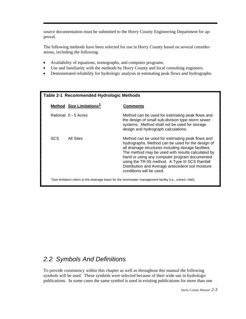
This Page Intentionally Left Blank 2.1 Hydrologic Methods Many hydrologic methods are available. The following methods are recommended and the circumstances for their use are listed in Table 2-1 below. If other methods are used, complete
Horry County Manual 2-3
source documentation must be submitted to the Horry County Engineering Department for ap-proval. The following methods have been selected for use in Horry County based on several consider-ations, including the following. • Availability of equations, nomographs, and computer programs. • Use and familiarity with the methods by Horry County and local consulting engineers. • Demonstrated reliability for hydrologic analysis in estimating peak flows and hydrographs. Table 2-1 Recommended Hydrologic Methods Method Size Limitations1 Comments Rational 0 - 5 Acres Method can be used for estimating peak flows and
the design of small sub-division type storm sewer systems. Method shall not be used for storage design and hydrograph calculations.
SCS All Sites Method can be used for estimating peak flows and
hydrographs. Method can be used for the design of all drainage structures including storage facilities. The method may be used with results calculated by hand or using any computer program documented using the TR-55 method. A Type III SCS Rainfall Distribution and Average antecedent soil moisture conditions will be used.
1Size limitation refers to the drainage basin for the stormwater management facility (i.e., culvert, inlet).
2.2 Symbols And Definitions To provide consistency within this chapter as well as throughout this manual the following symbols will be used. These symbols were selected because of their wide use in hydrologic publications. In some cases the same symbol is used in existing publications for more than one

2-4 Horry County Manual
definition. Where this occurs in this chapter, the symbol will be defined where it occurs in the text or equations.
Table 2-2 Symbols And Definitions Symbol Definition Units A or a Drainage area acres Af Channel flow area ft2 B Channel bottom width ft C Runoff coefficient - Cf Frequency factor - CN SCS-runoff curve number - D Depth of flow ft d Time interval hours F Pond and swamp adjustment factor - I Runoff intensity in./hr I Percent of impervious cover % Ia Initial abstraction from total rainfall in L Flow length ft n Manning roughness coefficient - P Accumulated rainfall in Pw Wetted perimeter ft Q Rate of runoff cfs q Storm runoff during a time interval in qu Unit peak discharge cfs/mi2/in qp Peak rate of discharge cfs R or r Hydraulic radius ft S or Y Ground slope ft/ft or % S Potential maximum retention in S or s Slope of hydraulic grade line ft/ft SCS Soil Conservation Service - T Channel top width ft TL or T Lag time hours Tt Travel time hours t C Time of concentration min V Velocity ft/s
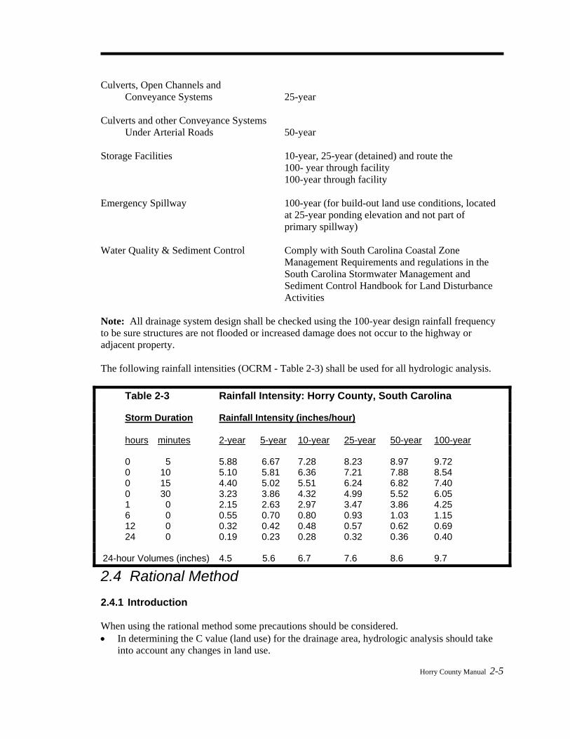
2.3 Design Frequency And Rainfall Following are the design frequencies to be used for the design of different stormwater manage-ment facilities. Stormwater Management Facility Design Frequency
Horry County Manual 2-5
Culverts, Open Channels and Conveyance Systems 25-year Culverts and other Conveyance Systems Under Arterial Roads 50-year Storage Facilities 10-year, 25-year (detained) and route the 100- year through facility 100-year through facility Emergency Spillway 100-year (for build-out land use conditions, located at 25-year ponding elevation and not part of primary spillway) Water Quality & Sediment Control Comply with South Carolina Coastal Zone Management Requirements and regulations in the South Carolina Stormwater Management and Sediment Control Handbook for Land Disturbance Activities Note: All drainage system design shall be checked using the 100-year design rainfall frequency to be sure structures are not flooded or increased damage does not occur to the highway or adjacent property. The following rainfall intensities (OCRM - Table 2-3) shall be used for all hydrologic analysis. Table 2-3 Rainfall Intensity: Horry County, South Carolina Storm Duration Rainfall Intensity (inches/hour) hours minutes 2-year 5-year 10-year 25-year 50-year 100-year 0 5 5.88 6.67 7.28 8.23 8.97 9.72 0 10 5.10 5.81 6.36 7.21 7.88 8.54 0 15 4.40 5.02 5.51 6.24 6.82 7.40 0 30 3.23 3.86 4.32 4.99 5.52 6.05 1 0 2.15 2.63 2.97 3.47 3.86 4.25 6 0 0.55 0.70 0.80 0.93 1.03 1.15 12 0 0.32 0.42 0.48 0.57 0.62 0.69 24 0 0.19 0.23 0.28 0.32 0.36 0.40 24-hour Volumes (inches) 4.5 5.6 6.7 7.6 8.6 9.7
2.4 Rational Method 2.4.1 Introduction When using the rational method some precautions should be considered. • In determining the C value (land use) for the drainage area, hydrologic analysis should take
into account any changes in land use.
2-6 Horry County Manual
• Since the rational method uses a composite C value for the entire drainage area, if the distribution of land uses within the drainage basin will affect the results of hydrologic analysis, then the basin should be divided into sub-drainage basins for analysis.
• The graphs, and tables included in this section are given to assist the engineer in applying the rational method. The engineer should use good engineering judgment in applying these design aids and should make appropriate adjustments when specific site characteristics dictate that these adjustments are appropriate.
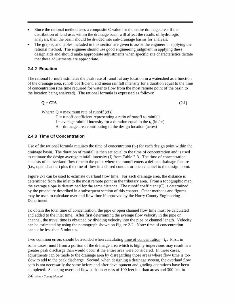
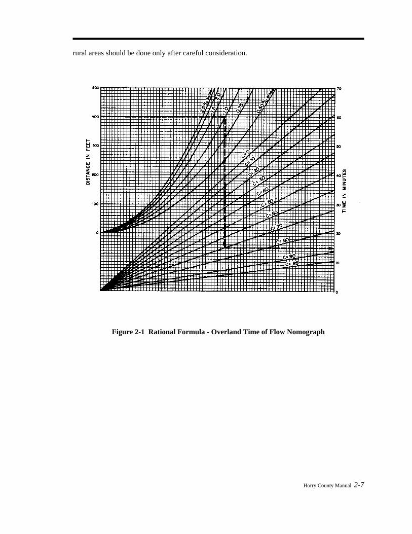
2.4.2 Equation The rational formula estimates the peak rate of runoff at any location in a watershed as a function of the drainage area, runoff coefficient, and mean rainfall intensity for a duration equal to the time of concentration (the time required for water to flow from the most remote point of the basin to the location being analyzed). The rational formula is expressed as follows: Q = CIA (2.1) Where: Q = maximum rate of runoff (cfs) C = runoff coefficient representing a ratio of runoff to rainfall I = average rainfall intensity for a duration equal to the tC (in./hr) A = drainage area contributing to the design location (acres) 2.4.3 Time Of Concentration Use of the rational formula requires the time of concentration (tc) for each design point within the drainage basin. The duration of rainfall is then set equal to the time of concentration and is used to estimate the design average rainfall intensity (I) from Table 2-3. The time of concentration consists of an overland flow time to the point where the runoff enters a defined drainage feature (i.e., open channel) plus the time of flow in a closed conduit or open channel to the design point. Figure 2-1 can be used to estimate overland flow time. For each drainage area, the distance is determined from the inlet to the most remote point in the tributary area. From a topographic map, the average slope is determined for the same distance. The runoff coefficient (C) is determined by the procedure described in a subsequent section of this chapter. Other methods and figures may be used to calculate overland flow time if approved by the Horry County Engineering Department. To obtain the total time of concentration, the pipe or open channel flow time must be calculated and added to the inlet time. After first determining the average flow velocity in the pipe or channel, the travel time is obtained by dividing velocity into the pipe or channel length. Velocity can be estimated by using the nomograph shown on Figure 2-2. Note: time of concentration cannot be less than 5 minutes. Two common errors should be avoided when calculating time of concentration - tc. First, in some cases runoff from a portion of the drainage area which is highly impervious may result in a greater peak discharge than would occur if the entire area were considered. In these cases, adjustments can be made to the drainage area by disregarding those areas where flow time is too slow to add to the peak discharge. Second, when designing a drainage system, the overland flow path is not necessarily the same before and after development and grading operations have been completed. Selecting overland flow paths in excess of 100 feet in urban areas and 300 feet in
Horry County Manual 2-7
rural areas should be done only after careful consideration.
Figure 2-1 Rational Formula - Overland Time of Flow Nomograph
2-8 Horry County Manual
Figure 2-2 Manning’s Equation Nomograph
Horry County Manual 2-9
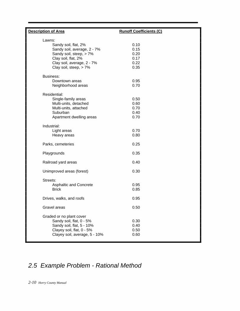
2.4.4 Rainfall Intensity The rainfall intensity (I) is the average rainfall rate in inches/hour for a duration equal to the time of concentration for a selected return period. Once a particular return period has been selected for design and a time of concentration calculated for the drainage area, the rainfall intensity can be determined from Rainfall-Intensity-Duration data. Table 2-3 gives the data for Horry County. Straight-line interpolation can be used to obtain rainfall intensity values for storm durations between the values given in Table 2-3. 2.4.5 Runoff Coefficient The runoff coefficient (C) is the variable of the rational method least susceptible to precise deter-mination and requires judgment and understanding on the part of the design engineer. While engineering judgment will always be required in the selection of runoff coefficients, typical coefficients represent the integrated effects of many drainage basin parameters. Table 2-4 gives the recommended runoff coefficients for the Rational Method. 2.4.6 Composite Coefficients It is often desirable to develop a composite runoff coefficient based on the percentage of different types of surfaces in the drainage areas. Composites can be made with the values from Table 2-4 by using percentages of different land uses. In addition, more detailed composites can be made with coefficients for different surface types such as roofs, asphalt, and concrete streets, drives and walks. The composite procedure can be applied to an entire drainage area or to typical "sample" blocks, as a guide to the selection of reasonable values of the coefficient for an entire area. It should be remembered that the rational method assumes that all land uses within a drainage area are uniformly distributed throughout the area. If it is important to locate a specific land use within the drainage area then another hydrologic method should be used where hydrographs can be generated and routed through the drainage system.
Table 2-4 Recommended Runoff Coefficient Values
2-10 Horry County Manual
Description of Area Runoff Coefficients (C) Lawns: Sandy soil, flat, 2% 0.10 Sandy soil, average, 2 - 7% 0.15 Sandy soil, steep, > 7% 0.20 Clay soil, flat, 2% 0.17 Clay soil, average, 2 - 7% 0.22 Clay soil, steep, > 7% 0.35 Business: Downtown areas 0.95 Neighborhood areas 0.70 Residential: Single-family areas 0.50 Multi-units, detached 0.60 Multi-units, attached 0.70 Suburban 0.40 Apartment dwelling areas 0.70 Industrial: Light areas 0.70 Heavy areas 0.80 Parks, cemeteries 0.25 Playgrounds 0.35 Railroad yard areas 0.40 Unimproved areas (forest) 0.30 Streets: Asphaltic and Concrete 0.95 Brick 0.85 Drives, walks, and roofs 0.95 Gravel areas 0.50 Graded or no plant cover Sandy soil, flat, 0 - 5% 0.30 Sandy soil, flat, 5 - 10% 0.40 Clayey soil, flat, 0 - 5% 0.50 Clayey soil, average, 5 - 10% 0.60
2.5 Example Problem - Rational Method
Horry County Manual 2-11
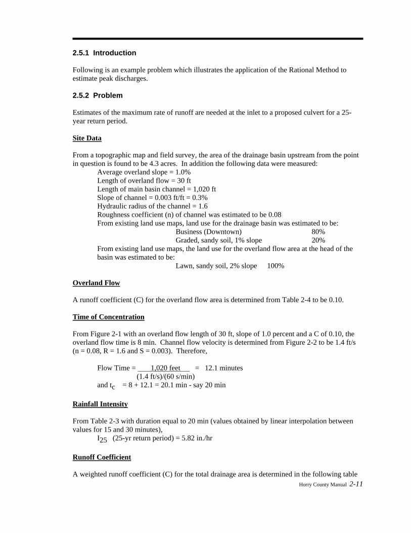
2.5.1 Introduction Following is an example problem which illustrates the application of the Rational Method to estimate peak discharges. 2.5.2 Problem Estimates of the maximum rate of runoff are needed at the inlet to a proposed culvert for a 25-year return period. Site Data From a topographic map and field survey, the area of the drainage basin upstream from the point in question is found to be 4.3 acres. In addition the following data were measured: Average overland slope = 1.0% Length of overland flow = 30 ft Length of main basin channel = 1,020 ft Slope of channel = 0.003 ft/ft = 0.3% Hydraulic radius of the channel = 1.6 Roughness coefficient (n) of channel was estimated to be 0.08 From existing land use maps, land use for the drainage basin was estimated to be:
Business (Downtown) 80% Graded, sandy soil, 1% slope 20%
From existing land use maps, the land use for the overland flow area at the head of the basin was estimated to be: Lawn, sandy soil, 2% slope 100%
Overland Flow A runoff coefficient (C) for the overland flow area is determined from Table 2-4 to be 0.10. Time of Concentration From Figure 2-1 with an overland flow length of 30 ft, slope of 1.0 percent and a C of 0.10, the overland flow time is 8 min. Channel flow velocity is determined from Figure 2-2 to be 1.4 ft/s (n = 0.08, R = 1.6 and S = 0.003). Therefore, Flow Time = 1,020 feet = 12.1 minutes (1.4 ft/s)/(60 s/min) and tc = 8 + 12.1 = 20.1 min - say 20 min Rainfall Intensity From Table 2-3 with duration equal to 20 min (values obtained by linear interpolation between values for 15 and 30 minutes), I25 (25-yr return period) = 5.82 in./hr Runoff Coefficient A weighted runoff coefficient (C) for the total drainage area is determined in the following table
2-12 Horry County Manual
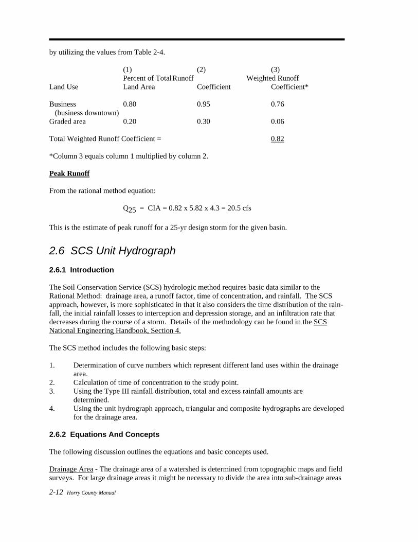
by utilizing the values from Table 2-4. (1) (2) (3) Percent of Total Runoff Weighted Runoff Land Use Land Area Coefficient Coefficient* Business 0.80 0.95 0.76 (business downtown) Graded area 0.20 0.30 0.06
Total Weighted Runoff Coefficient = 0.82 *Column 3 equals column 1 multiplied by column 2. Peak Runoff From the rational method equation: Q25 = CIA = 0.82 x 5.82 x 4.3 = 20.5 cfs This is the estimate of peak runoff for a 25-yr design storm for the given basin. 2.6 SCS Unit Hydrograph 2.6.1 Introduction The Soil Conservation Service (SCS) hydrologic method requires basic data similar to the Rational Method: drainage area, a runoff factor, time of concentration, and rainfall. The SCS approach, however, is more sophisticated in that it also considers the time distribution of the rain-fall, the initial rainfall losses to interception and depression storage, and an infiltration rate that decreases during the course of a storm. Details of the methodology can be found in the SCS National Engineering Handbook, Section 4. The SCS method includes the following basic steps: 1. Determination of curve numbers which represent different land uses within the drainage
area. 2. Calculation of time of concentration to the study point. 3. Using the Type III rainfall distribution, total and excess rainfall amounts are determined. 4. Using the unit hydrograph approach, triangular and composite hydrographs are developed
for the drainage area. 2.6.2 Equations And Concepts The following discussion outlines the equations and basic concepts used. Drainage Area - The drainage area of a watershed is determined from topographic maps and field surveys. For large drainage areas it might be necessary to divide the area into sub-drainage areas
Horry County Manual 2-13
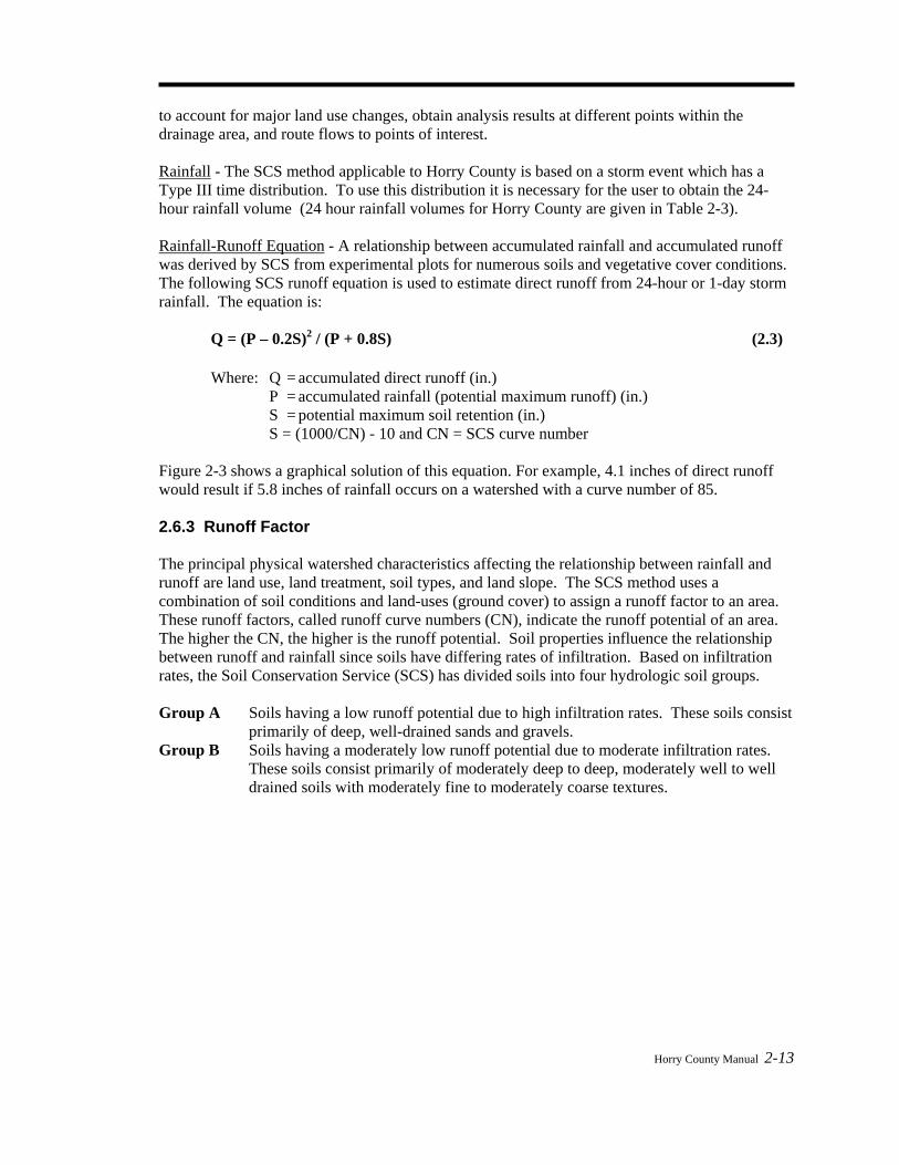
to account for major land use changes, obtain analysis results at different points within the drainage area, and route flows to points of interest. Rainfall - The SCS method applicable to Horry County is based on a storm event which has a Type III time distribution. To use this distribution it is necessary for the user to obtain the 24-hour rainfall volume (24 hour rainfall volumes for Horry County are given in Table 2-3). Rainfall-Runoff Equation - A relationship between accumulated rainfall and accumulated runoff was derived by SCS from experimental plots for numerous soils and vegetative cover conditions. The following SCS runoff equation is used to estimate direct runoff from 24-hour or 1-day storm rainfall. The equation is:
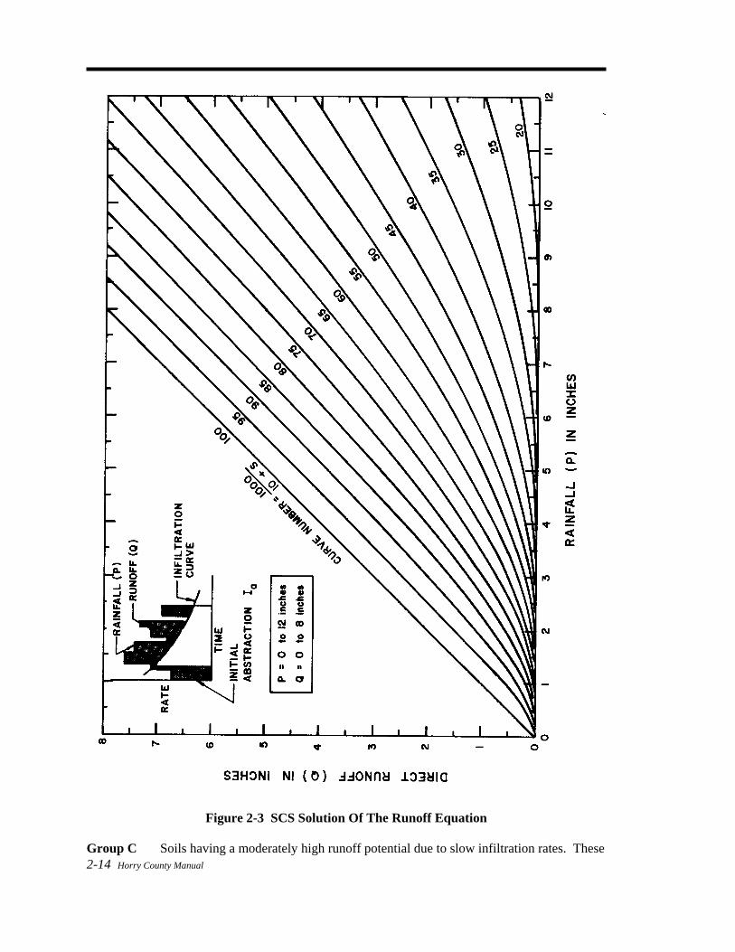
Q = (P – 0.2S)2 / (P + 0.8S) (2.3) Where: Q = accumulated direct runoff (in.)
P = accumulated rainfall (potential maximum runoff) (in.) S = potential maximum soil retention (in.)
S = (1000/CN) - 10 and CN = SCS curve number Figure 2-3 shows a graphical solution of this equation. For example, 4.1 inches of direct runoff would result if 5.8 inches of rainfall occurs on a watershed with a curve number of 85. 2.6.3 Runoff Factor The principal physical watershed characteristics affecting the relationship between rainfall and runoff are land use, land treatment, soil types, and land slope. The SCS method uses a combination of soil conditions and land-uses (ground cover) to assign a runoff factor to an area. These runoff factors, called runoff curve numbers (CN), indicate the runoff potential of an area. The higher the CN, the higher is the runoff potential. Soil properties influence the relationship between runoff and rainfall since soils have differing rates of infiltration. Based on infiltration rates, the Soil Conservation Service (SCS) has divided soils into four hydrologic soil groups. Group A Soils having a low runoff potential due to high infiltration rates. These soils consist
primarily of deep, well-drained sands and gravels. Group B Soils having a moderately low runoff potential due to moderate infiltration rates.
These soils consist primarily of moderately deep to deep, moderately well to well drained soils with moderately fine to moderately coarse textures.
2-14 Horry County Manual
Figure 2-3 SCS Solution Of The Runoff Equation Group C Soils having a moderately high runoff potential due to slow infiltration rates. These

Horry County Manual 2-15
soils consist primarily of soils in which a layer exists near the surface that impedes the downward movement of water or soils with moderately fine to fine texture.
Group D Soils having a high runoff potential due to very slow infiltration rates. These soils consist primarily of clays with high swelling potential, soils with permanently high water tables, soils with a claypan or clay layer at or near the surface, and shallow soils over nearly impervious parent material.
A list of soils for Horry County and their hydrologic classification is presented in Table 2-5. Soil Survey maps can be obtained from local SCS (NRCS) office.
Table 2-5 Hydrologic Soils Groups For Horry County Series Name Hydrologic Group Series Name Hydrologic Group Bladen D Lynn Haven B/D Blanton A Meggett D Bohicket D Nankina B/D Brookman D Nansemond C Centenary A Newhan C Chisolm A Norfolk B Coxville D Ogeechee B/D Duplin C Osier A/D Echaw A Pocomoke -Drained B Emporia C - Ponded B/D Eulonia C Rimini A Goldsboro B Rutlege B/D Hobcaw D Suffolk B Hobonny D Summerton B Johnston D Wahee D Kenansville A Witherbee A/D Lakeland A Woodington B/D Leon B/D Yauhannah B Lynchburg C Yemassee C Yonges D Note: B/D indicates the drained/undrained situation. Consideration should be given to the effects of urbanization on the natural hydrologic soil group. If heavy equipment can be expected to compact the soil during construction or if grading will mix the surface and subsurface soils, appropriate changes should be made in the soil group selected. Also runoff curve numbers vary with the antecedent soil moisture conditions. Average antecedent soil moisture conditions (AMC II) are recommended for all hydrologic analysis. Table 2-6 gives recommended curve number values for a range of different land uses. 2.6.4 Urban Modifications Several factors, such as the percentage of impervious area and the means of conveying runoff from impervious areas to the drainage system, should be considered in computing CN for urban areas. For example, do the impervious areas connect directly to the drainage system, or do they

2-16 Horry County Manual
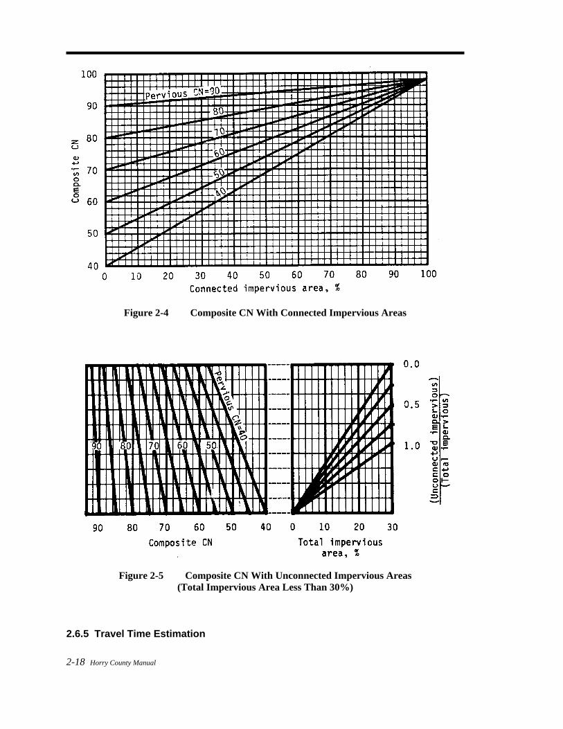
outlet onto lawns or other pervious areas where infiltration can occur? The curve number values given in Table 2-6 are based on directly connected impervious area. An impervious area is considered directly connected if runoff from it flows directly into the drainage system. It is also considered directly connected if runoff from it occurs as concentrated shallow flow that runs over pervious areas and then into a drainage system. It is possible that curve number values from urban areas could be reduced by not directly connecting impervious surfaces to the drainage system. The following discussion will give some guidance for adjusting curve numbers for different types of impervious areas. Connected Impervious Areas Urban CNs given in Table 2-6 were developed for typical land use relationships based on specific assumed percentages of impervious area. These CN values were developed on the assumptions that: (a) pervious urban areas are equivalent to pasture in good hydrologic condition, and (b) impervious areas have a CN of 98 and are directly connected to the drainage system. Some assumed percentages of impervious area are shown in Table 2-6. If all of the impervious area is directly connected to the drainage system, but the impervious area percentages or the pervious land use assumptions in Table 2-6 are not applicable, use Figure 2-4 to compute a composite CN. For example, Table 2-6 gives a CN of 70 for a 1/2-acre lot in hydrologic soil group B, with an assumed impervious area of 25 percent. However, if the lot has 20 percent impervious area and a pervious area CN of 61, the composite CN obtained from Figure 2-4 is 68. The CN difference between 70 and 68 reflects the difference in percent impervious area. Unconnected Impervious Areas Runoff from these areas is spread over a pervious area as sheet flow. To determine CN when all or part of the impervious area is not directly connected to the drainage system, (1) use Figure 2-5 if total impervious area is less then 30 percent or (2) use Figure 2-4 if the total impervious area is equal to or greater than 30 percent, because the absorptive capacity of the remaining pervious areas will not significantly affect runoff. When impervious area is less than 30 percent, obtain the composite CN by entering the right half of Figure 2-5 with the percentage of total impervious area and the ratio of total unconnected impervious area to total impervious area. Then move left to the appropriate pervious CN and read down to find the composite CN. For example, for a 1/2-acre lot with 20 percent total impervious area (75 percent of which is unconnected) and pervious CN of 61, the composite CN from Figure 2-5 is 66. If all of the impervious area is connected, the resulting CN (from Figure 2-4) would be 68.
Table 2-6 Runoff Curve Numbers1Cover description Curve numbers for hydrologic soil groups Cover type and Average percent A B C D hydrologic condition impervious area2
Horry County Manual 2-17
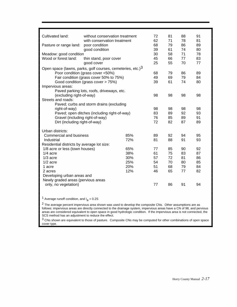
Cultivated land: without conservation treatment 72 81 88 91 with conservation treatment 62 71 78 81 Pasture or range land: poor condition 68 79 86 89 good condition 39 61 74 80 Meadow: good condition 30 58 71 78 Wood or forest land: thin stand, poor cover 45 66 77 83 good cover 25 55 70 77 Open space (lawns, parks, golf courses, cemeteries, etc.)3 Poor condition (grass cover <50%) 68 79 86 89 Fair condition (grass cover 50% to 75%) 49 69 79 84 Good condition (grass cover > 75%) 39 61 74 80 Impervious areas: Paved parking lots, roofs, driveways, etc. (excluding right-of-way) 98 98 98 98 Streets and roads: Paved; curbs and storm drains (excluding right-of-way) 98 98 98 98 Paved; open ditches (including right-of-way) 83 89 92 93 Gravel (including right-of-way) 76 85 89 91 Dirt (including right-of-way) 72 82 87 89 Urban districts: Commercial and business 85% 89 92 94 95 Industrial 72% 81 88 91 93 Residential districts by average lot size: 1/8 acre or less (town houses) 65% 77 85 90 92 1/4 acre 38% 61 75 83 87 1/3 acre 30% 57 72 81 86 1/2 acre 25% 54 70 80 85 1 acre 20% 51 68 79 84 2 acres 12% 46 65 77 82 Developing urban areas and Newly graded areas (pervious areas only, no vegetation) 77 86 91 94 1 Average runoff condition, and Ia = 0.2S 2 The average percent impervious area shown was used to develop the composite CNs. Other assumptions are as follows: impervious areas are directly connected to the drainage system, impervious areas have a CN of 98, and pervious areas are considered equivalent to open space in good hydrologic condition. If the impervious area is not connected, the SCS method has an adjustment to reduce the effect. 3 CNs shown are equivalent to those of pasture. Composite CNs may be computed for other combinations of open space cover type.
2-18 Horry County Manual
Figure 2-4 Composite CN With Connected Impervious Areas
Figure 2-5 Composite CN With Unconnected Impervious Areas
(Total Impervious Area Less Than 30%)
2.6.5 Travel Time Estimation
Horry County Manual 2-19
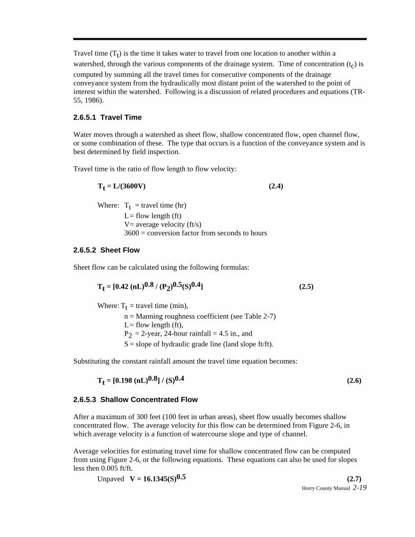
Travel time (Tt) is the time it takes water to travel from one location to another within a watershed, through the various components of the drainage system. Time of concentration (tc) is computed by summing all the travel times for consecutive components of the drainage conveyance system from the hydraulically most distant point of the watershed to the point of interest within the watershed. Following is a discussion of related procedures and equations (TR-55, 1986). 2.6.5.1 Travel Time Water moves through a watershed as sheet flow, shallow concentrated flow, open channel flow, or some combination of these. The type that occurs is a function of the conveyance system and is best determined by field inspection.
Travel time is the ratio of flow length to flow velocity:
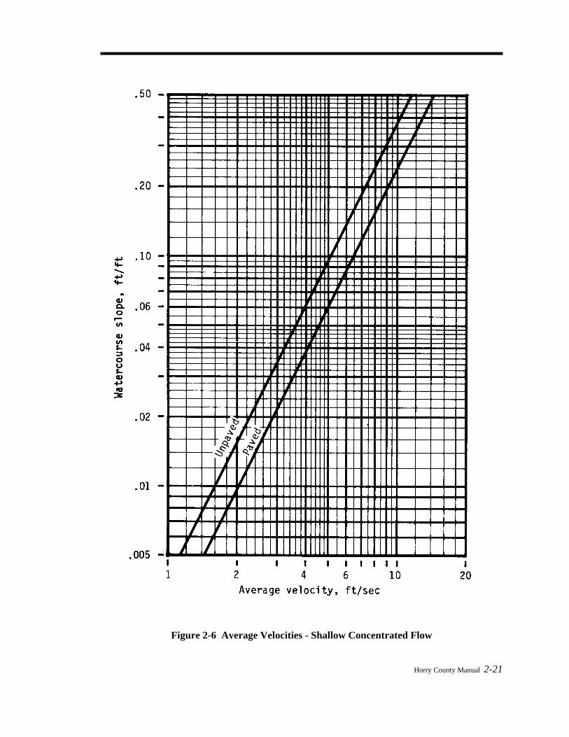
Tt = L/(3600V) (2.4) Where: Tt = travel time (hr) L = flow length (ft) V = average velocity (ft/s) 3600 = conversion factor from seconds to hours 2.6.5.2 Sheet Flow Sheet flow can be calculated using the following formulas: Tt = [0.42 (nL)0.8 / (P2)0.5(S)0.4] (2.5) Where: Tt = travel time (min), n = Manning roughness coefficient (see Table 2-7) L = flow length (ft), P2 = 2-year, 24-hour rainfall = 4.5 in., and S = slope of hydraulic grade line (land slope ft/ft). Substituting the constant rainfall amount the travel time equation becomes: Tt = [0.198 (nL)0.8] / (S)0.4 (2.6) 2.6.5.3 Shallow Concentrated Flow After a maximum of 300 feet (100 feet in urban areas), sheet flow usually becomes shallow concentrated flow. The average velocity for this flow can be determined from Figure 2-6, in which average velocity is a function of watercourse slope and type of channel. Average velocities for estimating travel time for shallow concentrated flow can be computed from using Figure 2-6, or the following equations. These equations can also be used for slopes less then 0.005 ft/ft.
Unpaved V = 16.1345(S)0.5 (2.7)
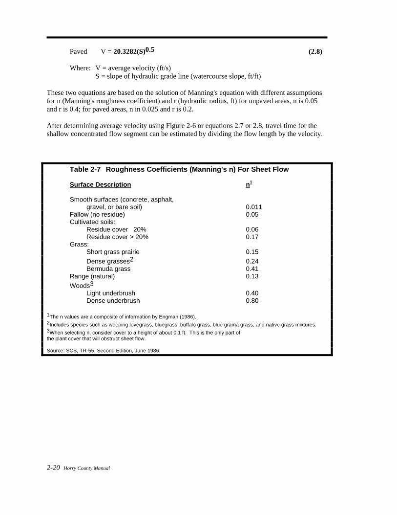
2-20 Horry County Manual
Paved V = 20.3282(S)0.5 (2.8) Where: V = average velocity (ft/s) S = slope of hydraulic grade line (watercourse slope, ft/ft) These two equations are based on the solution of Manning's equation with different assumptions for n (Manning's roughness coefficient) and r (hydraulic radius, ft) for unpaved areas, n is 0.05 and r is 0.4; for paved areas, n in 0.025 and r is 0.2. After determining average velocity using Figure 2-6 or equations 2.7 or 2.8, travel time for the shallow concentrated flow segment can be estimated by dividing the flow length by the velocity. Table 2-7 Roughness Coefficients (Manning's n) For Sheet Flow Surface Description n1
Smooth surfaces (concrete, asphalt, gravel, or bare soil) 0.011 Fallow (no residue) 0.05 Cultivated soils: Residue cover 20% 0.06 Residue cover > 20% 0.17 Grass: Short grass prairie 0.15 Dense grasses2 0.24 Bermuda grass 0.41 Range (natural) 0.13 Woods3 Light underbrush 0.40 Dense underbrush 0.80 1The n values are a composite of information by Engman (1986). 2Includes species such as weeping lovegrass, bluegrass, buffalo grass, blue grama grass, and native grass mixtures. 3When selecting n, consider cover to a height of about 0.1 ft. This is the only part of the plant cover that will obstruct sheet flow. Source: SCS, TR-55, Second Edition, June 1986.
Horry County Manual 2-21
Figure 2-6 Average Velocities - Shallow Concentrated Flow
2-22 Horry County Manual
2.6.5.4 Open Channels Open channels are assumed to begin where surveyed cross section information has been obtained, where channels are visible on aerial photographs, or where blue lines (indicating streams) appear on United States Geological Survey (USGS) quadrangle sheets. Manning's equation or water surface profile information can be used to estimate average flow velocity. Average flow velocity is usually determined for bank-full elevation. Manning's equation is V = [1.49 (r)2/3 (s)1/2] / n (2.9) Where: V = average velocity (ft/s) r = hydraulic radius (ft) and is equal to a/pw
a = cross sectional flow area (ft2) pw = wetted perimeter (ft) s = slope of the hydraulic grade line (ft/ft) n = Manning's roughness coefficient for open channel flow After average velocity is computed using equation 2.9, Tt for the channel segment can be estimated by dividing the flow length by the velocity. Velocity in channels should be calculated from the Manning equation. Cross sections from all channels that have been field checked should be used in the calculations. This is particularly true of areas below dams or other flow control structures. 2.6.5.5 Limitations
• Equations in this section should not be used for sheet flow longer than 300 feet (100 feet in urban areas).
• In watersheds with storm sewers, carefully identify the appropriate hydraulic flow path to estimate tc.
• A culvert or bridge can act as a reservoir outlet if there is significant storage, protected by recorded easements, behind it. Detailed storage routing procedures should be used to determine the outflow through the culvert.
2.6.6 Triangular Hydrograph Equation The triangular hydrograph is a practical representation of excess runoff with only one rise, one peak, and one recession. Its geometric makeup can be easily described mathematically, which makes it very useful in the process of estimating discharge rates, and produces results that are sufficiently accurate for most drainage facility designs. The SCS developed the following equation to estimate the peak rate of discharge for an increment of runoff:
qp = (K A (q)) / (d/2 + TL) (2.10) Where: qp= peak rate of discharge (cfs) K = 256 for pre-development conditions and = 323 for post-development conditions
Unless prior approval is received from Horry County to use a different value for the constant K.
Horry County Manual 2-23
A = area (mi2) q = storm runoff volume during time interval (in.) d = rainfall time increment TL= watershed lag time ( TL = 0.6 tc) (hr)
Tp= time to peak (d/2 + TL) (hr) Tb= time of base (2.67Tp) (hr)
2.7 Simplified SCS Method 2.7.1 Overview The following SCS procedures were taken from the SCS Technical Release 55 (TR-55) which presents simplified procedures to calculate storm runoff volume, peak rate of discharges and hydrographs. These procedures are applicable to small drainage areas and include provisions to account for urbanization. The following procedures outline the use of the SCS-TR 55 method. 2.7.2 Peak Discharges The SCS peak discharge method is applicable for estimating the peak runoff rate from watersheds with a homogeneous land use. The following method is based on the results of computer analyses performed using TR-20, "Computer Program for Project Formulation - Hydrology" (SCS 1983). The peak discharge equation is:
Qp = quAQFp (2.11) Where: Qp = peak discharge (cfs)
qu = unit peak discharge (cfs/mi2/in)
A = drainage area (mi2) Q = runoff (in) Fp = pond and swamp adjustment factor The input requirements for this method are as follows:
1. Tc - hours
2. Drainage area - mi2 3. Type III rainfall distribution 4. 24-hour design rainfall 5. CN value 6. Pond and Swamp adjustment factor (If pond and swamp areas are spread
throughout the watershed and are not considered in the Tc computation, an adjustment is needed.)
2-24 Horry County Manual
2.7.3 Computations Computations for the peak discharge method proceed as follows: 1. The 24-hour rainfall depth is in Table 2-3 for the selected return frequency. 2. The runoff curve number, CN, is estimated from Table 2-6 and direct runoff, Q, is
estimated from Figure 2-3. Determine if urban modifications of CN are appropriate. 3. The CN value is used to determine the initial abstraction, Ia, from Table 2-8, and the ratio
Ia/P is then computed. (P = accumulated 24-hour rainfall or potential maximum runoff.) 4. The watershed time of concentration is computed using the procedures in Section 2.6.5
and is used with the ratio Ia/P to obtain the unit peak discharge, qu, from Figure 2-7. If the ratio Ia/P lies outside the range shown in Figure 2-7, either the limiting values or another peak discharge method should be used.
5. The pond and swamp adjustment factor, Fp, is estimated from below: Pond & Swamp Areas (%*) Fp 0 1.00 0.2 0.97 1.0 0.87 3.0 0.75 5.0 0.72 *Percent of entire drainage basin 6. The peak runoff rate is computed using equation 2.11. 2.7.4 Limitations The accuracy of the peak discharge method is subject to specific limitations, including the following: 1. The watershed must be hydrologically homogeneous and describable by a single CN
value. 2. The watershed may have only one main stream, or if more than one, the individual
branches must have nearly equal time of concentrations. 3. Hydrologic routing cannot be considered. 4. The pond and swamp adjustment factor, Fp, applies only to areas located away from the
main flow path. 5. Accuracy is reduced if the ratio Ia/P is outside the range given in Figure 2-7.
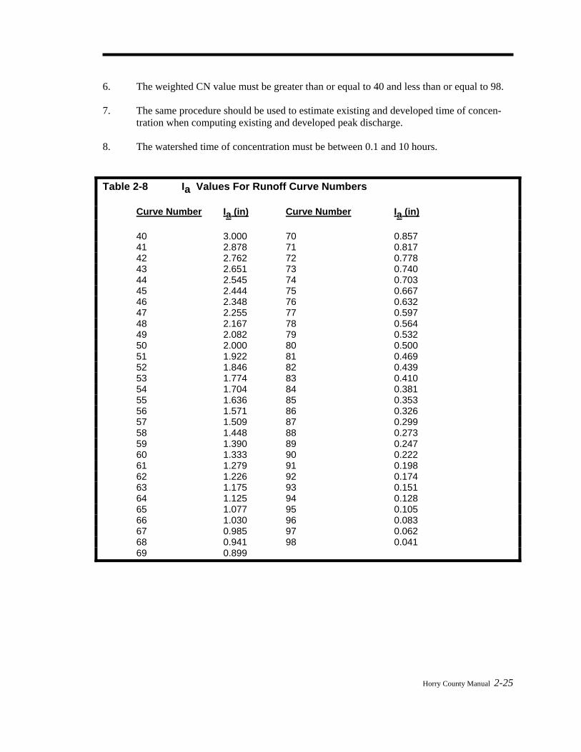
Horry County Manual 2-25
6. The weighted CN value must be greater than or equal to 40 and less than or equal to 98. 7. The same procedure should be used to estimate existing and developed time of concen-
tration when computing existing and developed peak discharge. 8. The watershed time of concentration must be between 0.1 and 10 hours. Table 2-8 Ia Values For Runoff Curve Numbers Curve Number Ia (in) Curve Number Ia (in) 40 3.000 70 0.857 41 2.878 71 0.817 42 2.762 72 0.778 43 2.651 73 0.740 44 2.545 74 0.703 45 2.444 75 0.667 46 2.348 76 0.632 47 2.255 77 0.597 48 2.167 78 0.564 49 2.082 79 0.532 50 2.000 80 0.500 51 1.922 81 0.469 52 1.846 82 0.439 53 1.774 83 0.410 54 1.704 84 0.381 55 1.636 85 0.353 56 1.571 86 0.326 57 1.509 87 0.299 58 1.448 88 0.273 59 1.390 89 0.247 60 1.333 90 0.222 61 1.279 91 0.198 62 1.226 92 0.174 63 1.175 93 0.151 64 1.125 94 0.128 65 1.077 95 0.105 66 1.030 96 0.083 67 0.985 97 0.062 68 0.941 98 0.041 69 0.899
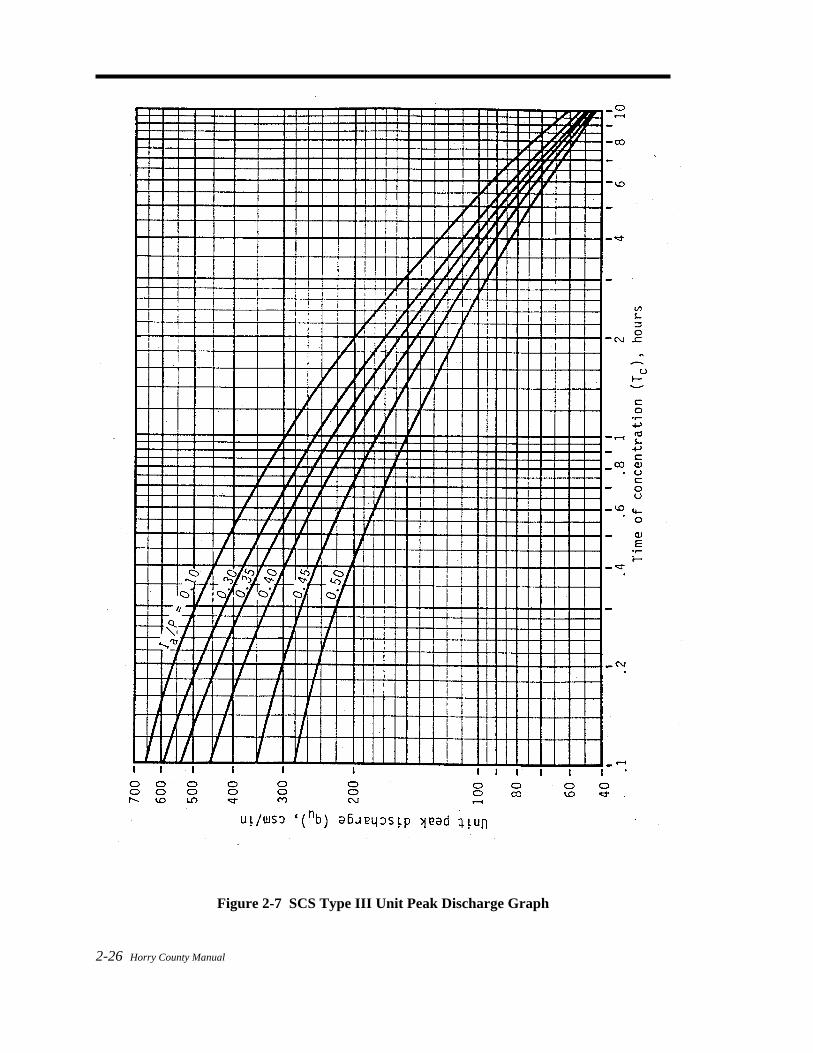
2-26 Horry County Manual
Figure 2-7 SCS Type III Unit Peak Discharge Graph

Horry County Manual 2-27
2.7.5 Example Problem Compute the 25-year peak discharge for a 50-acre wooded watershed which will be developed as follows:
1. Forest land - good cover (hydrologic soil group B) = 10 ac. 2. Forest land - poor cover (hydrologic soil group D) = 10 ac. 3. Town house residential (hydrologic soil group B) = 20 ac. 4. Industrial development (hydrological soil group D) = 10 ac. Other data include: percentage of pond and swamp area = 0.20%. Computations 1. Calculate rainfall excess:
• The 25-year, 24-hour rainfall is 7.6 inches. • Composite weighted runoff coefficient is:
Dev. # Area % Total Cn Composite Cn
1 10 ac. 0.20 55 11.0 2 10 ac. 0.20 83 16.6 3 20 ac. 0.40 85 34.0 4 10 ac. 0.20 93 18.6
Total 50 ac. 1.00 80.2 use 80 Assume all impervious areas are directly connected so urban modifications are not justified.
* From Figure 2-3, Q = 5.4 inches
2. Calculate time of concentration
• The hydrologic flow path for this watershed = 2,000 ft.
Segment Type of Flow Length Slope (%)
1 Overland n = 0.24 40 ft. 0.5 % 2 Shallow channel 750 ft. 0.8 % 3 Main channel* 1,100 ft. 0.5 %
* For the main channel, n = 0.06 (estimated), width = 10 feet, depth = 2 feet,
rectangular channel. R = Cross-Sectional Area/Wetted Perimeter = 20/14 = 1.43 feet
• Segment 1 - Travel time from equation 2.6 with P2 = 4.5 in.
2-28 Horry County Manual
Tt = [0.198(0.24 x 40)0.8] / (0.005)0.4 Tt = 10.07 minutes
• Segment 2 - Travel time from Figure 2-6 or equation 2.7 V = 1.44 ft/sec (from equation 2.7) Tt = 750 / 60 (1.44) = 8.68 minutes
• Segment 3 - Using equation 2.9
V = (1.49/0.06) (1.43)0.67 (0.005)0.5 = 2.23 ft/sec Tt = 1100 / 60 (2.23) = 8.22 minutes
• Tc = 10.07 + 8.68 + 8.22 = 26.97 minutes (0.45 hours)
3. Calculate Ia/P for Composite Cn = 80, Ia = 0.500 (Table 2-8) Ia/P = (0.500 / 7.6) = 0.066
(Note: Use Ia/P = 0.10 which is the minimum value given in Figure 2-7) 4. Estimate unit discharge qu from Figure 2-7 (Tc = 0.45 hr) = 430 cfs 5. Calculate peak discharge with Fp = 0.97 using equation 2.11 Q25 = 430 (50/640) (5.4) (0.97) = 176 cfs 2.7.6 Hydrograph Generation In addition to estimating the peak discharge, the SCS method can be used to estimate the entire hydrograph from a drainage area. The Soil Conservation Service has developed a Tabular Hydrograph procedure that can be used to generate the hydrograph for small drainage areas (less than 2,000 acres). The Tabular Hydrograph procedure uses unit discharge hydrographs that have been generated for a series of time of concentrations. In addition, SCS has developed hydrograph procedures to be used to generate composite flood hydrographs. For the development of a hydrograph from a homogeneous developed drainage area and drainage areas which are not homogeneous, where hydrographs need to be generated from sub-areas and then routed and combined at a point downstream, the engineer is referred to the procedures outlined by the SCS in the 1986 version of TR-55 available from the National Technical Information Service in Spring-field, Virginia 22161. The catalog number for TR-55, "Urban Hydrology for Small Watersheds," is PB87-101580. Since most local engineers use computer program to generate hydrograph analysis, detailed hand procedures for hydrograph are not presented in this manual. The above reference gives the details of hydrograph generated for those who want a hand-calculated procedure. References
Horry County Manual 2-29
Federal Highway Administration. 1991. HYDRAIN Documentation.
U. S. Department of Agriculture, Soil Conservation Service, Engineering Division. 1986. Urban hydrology for small watersheds. Technical Release 55 (TR-55).
U. S. Department of Transportation, Federal Highway Administration. 1984. Hydrology. Hydraulic Engineering Circular No. 19.
Overton, D. E. and M. E. Meadows. 1976. Storm water modeling. Academic Press. New York, N.Y. pp. 58-88.
Water Resources Council Bulletin 17B. 1981. Guidelines for determining flood flow frequency.
Wright-McLaughlin Engineers. 1969. Urban storm drainage criteria manual. Vol. I and II. Prepared for the Denver Regional Council of Governments, Denver, Colorado.


HYDROLOGY 2
Chapter 2 - Hydrology 2B-1
CHAPTER
STORM DRAINAGE 3
SYSTEMS
Horry County Manual 3-1
CHAPTER
Chapter Table of Contents 3.1 Overview .................................................................................................................. 3-2
3.1.1 Introduction .................................................................................................... 3-3 3.1.2 Inlet Definition ............................................................................................... 3-3 3.1.3 Criteria ............................................................................................................ 3-3
3.2 Symbols And Definitions ........................................................................................ 3-4 3.3 Gutter Flow Calculations ....................................................................................... 3-4
3.3.1 Formula........................................................................................................... 3-4 3.3.2 Nomograph ..................................................................................................... 3-5 3.3.3 Manning's n Table .......................................................................................... 3-5 3.3.4 Uniform Cross Slope ...................................................................................... 3-5 3.3.5 Composite Gutter Sections ............................................................................. 3-7 3.3.6 Examples ...................................................................................................... 3-10
3.4 Grate Inlets Design ............................................................................................... 3-11 3.4.1 Types ............................................................................................................ 3-11 3.4.2 Grate Inlets On Grade................................................................................... 3-11 3.4.3 Grate Inlets In Sag ........................................................................................ 3-16
3.5 Curb Inlet Design.................................................................................................. 3-18 3.5.1 Curb Inlets On Grade.................................................................................... 3-18
3.5.1.1 Design Steps.................................................................................... 3-19 3.5.1.2 Example........................................................................................... 3-20
3.5.2 Curb Inlets In Sag ......................................................................................... 3-22 3.5.2.1 Design Steps.................................................................................... 3-23 3.5.2.2 Example............................................................................................ 3-26
3.6 Combination Inlets ............................................................................................... 3-27 3.6.1 On Grade....................................................................................................... 3-27 3.6.2 In Sag............................................................................................................ 3-27
3.7 Storm Drains ......................................................................................................... 3-27 3.7.1 Introduction .................................................................................................. 3-27 3.7.2 Design Criteria.............................................................................................. 3-28 3.7.3 Capacity ........................................................................................................ 3-28 3.7.4 Nomographs And Table................................................................................ 3-29 3.7.5 Hydraulic Grade Lines.................................................................................. 3-34 3.7.6 Minimum Grade ........................................................................................... 3-36 3.7.7 Storm Drain Storage ..................................................................................... 3-36 3.7.8 Design Procedures ........................................................................................ 3-36
References..................................................................................................................... 3-39

3-2 Horry County Manual
This Page Intentionally Left Blank 3.1 Overview

Horry County Manual 3-3
3.1.1 Introduction In this chapter, guidelines are given for evaluating roadway features and design criteria as they relate to gutter and inlet hydraulics and storm drain design. Procedures for performing gutter flow calculations are based on a modification of Manning's Equation. Inlet capacity calculations for grate and combination inlets are based on information contained in HEC-12 (USDOT, FHWA, 1984). Storm drain design is based on the use of the rational formula. 3.1.2 Inlet Definition There are three storm water inlet categories: curb opening inlets grated inlets combination inlets In addition, inlets may be classified as being on a continuous grade or in a sag. The term "continuous grade" refers to an inlet located on the street with a continuous slope past the inlet with water entering from one direction. The "sag" condition exists when the inlet is located at a low point and water enters from both directions. 3.1.3 Criteria Design Frequency 1. The 25-year design storm shall be used for conveyance systems and drainage designs. 2. The 50-year design storm shall be used for conveyance systems under arterial roads. Spread Limits Catch basins shall be spaced so that the spread in the street for the 25-year design flow shall not exceed the following, as measured from the face of the curb: (1) 8 feet if the street is classified as a Collector or Arterial (for 2 lane streets spread may extend to one-half of the travel lane, for 4 lane streets spread may extend across one travel lane); (2) 16 feet at any given section, but in no case greater than 10 feet on one side of the street, if the street is classified as a Local or Sub-Collector Street. Clogging Factor for Inlets 1. For grated inlets located in residential areas, a clogging factor of 25% shall be used in the
design of these systems. 2. For grated inlets located in commercial areas, a clogging factor of 0% shall be used. 3. For curb opening or open throat inlets located in either residential or commercial areas, a
clogging factor of 0% shall be used.

3-4 Horry County Manual
3.2 Symbols And Definitions To provide consistency within this chapter as well as throughout this manual the following symbols will be used. These symbols were selected because of their wide use in storm drainage publications. In some cases the same symbol is used in existing publications for more than one definition. Where this occurs in this chapter, the symbol will be defined where it occurs in the text or equations. Table 3-1 Symbols And Definitions Symbol Definition Units a Gutter depression in A Area of cross section ft2 d or D Depth of gutter flow at the curb line ft D Diameter of pipe ft Eo Ratio of frontal flow to total gutter flow Qw/Q -
g Acceleration due to gravity (32.2 ft/s2) ft/s2 h Height of curb opening inlet ft H Head loss ft K Loss coefficient - L or LT Length of curb opening inlet ft L Pipe length ft n Roughness coefficient in the modified Manning formula for triangular gutter flow - P Perimeter of grate opening, neglecting bars and side against curb ft Q Rate of discharge in gutter cfs Qi Intercepted flow cfs Qs Gutter capacity above the depressed section cfs S or Sx Cross Slope - Traverse slope ft/ft S or SL Longitudinal slope of pavement ft/ft Sf Friction slope ft/ft S'w Depression section slope ft/ft T Top width of water surface (spread on pavement) ft Ts Spread above depressed section ft V Velocity of flow ft/s W Width of depression for curb opening inlets ft Z T/d, reciprocal of the cross slope - 3.3 Gutter Flow Calculations 3.3.1 Formula The following form of Manning's Equation should be used to evaluate gutter flow hydraulics: Q = [0.56 / n] Sx5/3 S1/2 T8/3 (3.1) Where: Q = gutter flow rate (cfs) n = Manning's roughness coefficient
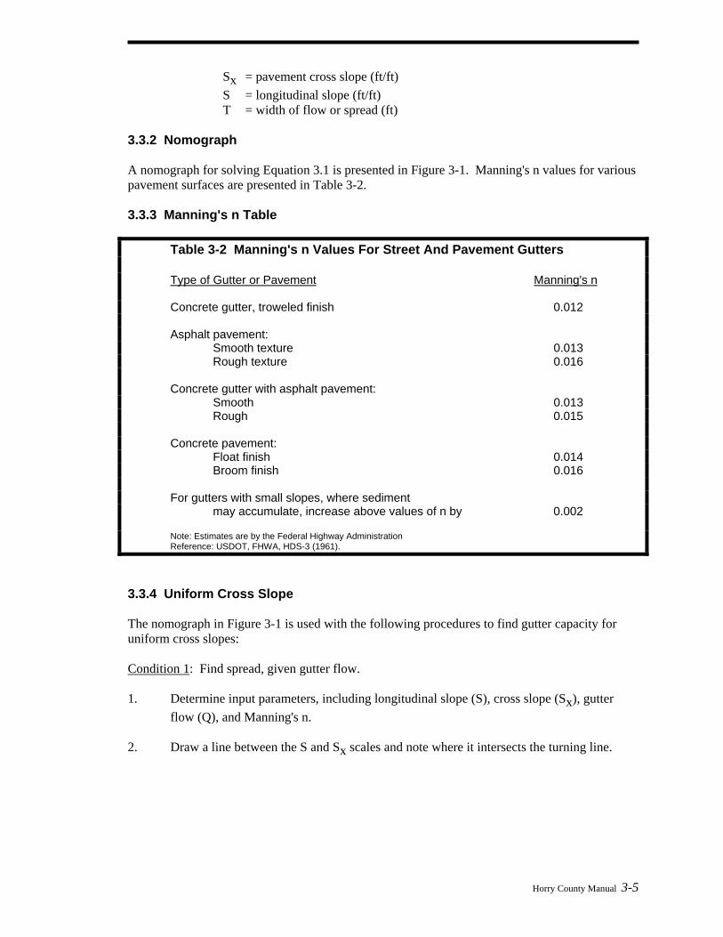
Horry County Manual 3-5
Sx = pavement cross slope (ft/ft) S = longitudinal slope (ft/ft) T = width of flow or spread (ft) 3.3.2 Nomograph A nomograph for solving Equation 3.1 is presented in Figure 3-1. Manning's n values for various pavement surfaces are presented in Table 3-2. 3.3.3 Manning's n Table Table 3-2 Manning's n Values For Street And Pavement Gutters Type of Gutter or Pavement Manning's n Concrete gutter, troweled finish 0.012 Asphalt pavement: Smooth texture 0.013 Rough texture 0.016 Concrete gutter with asphalt pavement: Smooth 0.013 Rough 0.015 Concrete pavement: Float finish 0.014 Broom finish 0.016 For gutters with small slopes, where sediment may accumulate, increase above values of n by 0.002 Note: Estimates are by the Federal Highwa Administration y Reference: USDOT, FHWA, HDS-3 (1961). 3.3.4 Uniform Cross Slope The nomograph in Figure 3-1 is used with the following procedures to find gutter capacity for uniform cross slopes: Condition 1: Find spread, given gutter flow. 1. Determine input parameters, including longitudinal slope (S), cross slope (Sx), gutter
flow (Q), and Manning's n. 2. Draw a line between the S and Sx scales and note where it intersects the turning line.
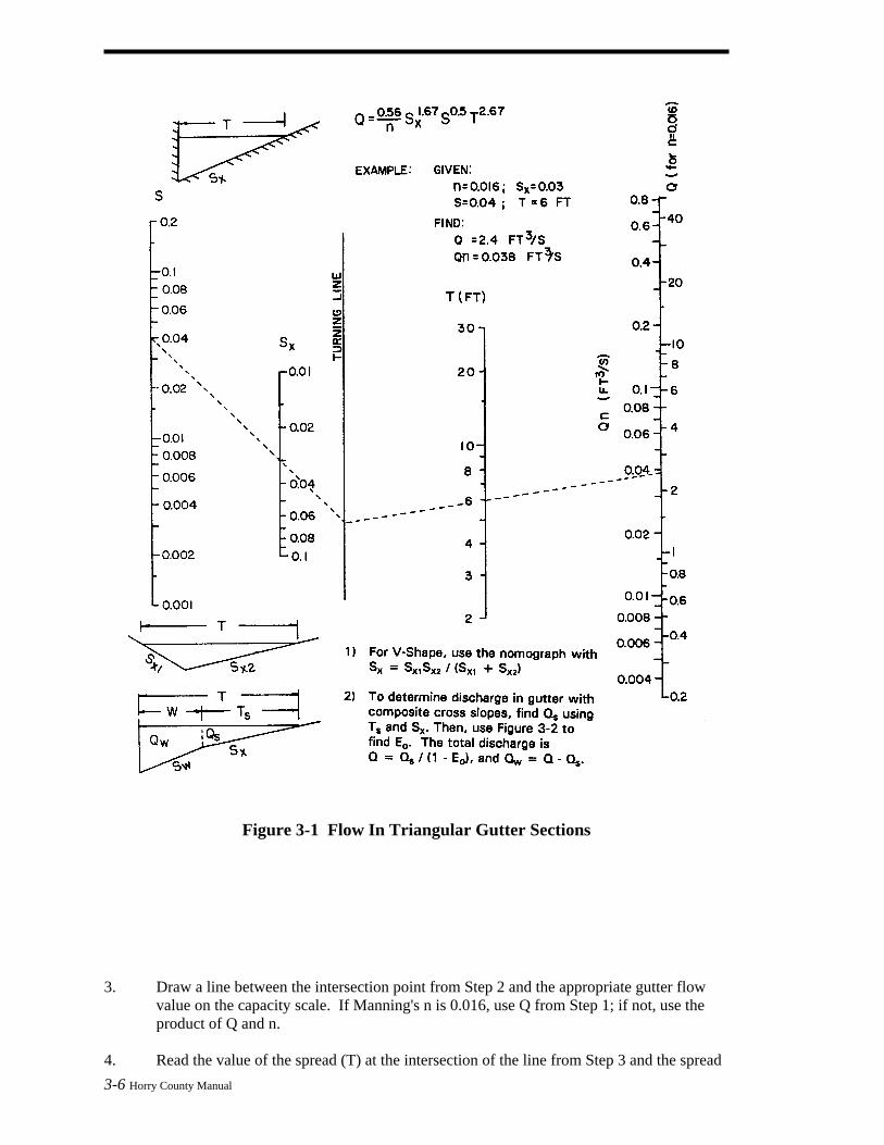
Figure 3-1 Flow In Triangular Gutter Sections
3. Draw a line between the intersection point from Step 2 and the appropriate gutter flow
value on the capacity scale. If Manning's n is 0.016, use Q from Step 1; if not, use the product of Q and n.
4. Read the value of the spread (T) at the intersection of the line from Step 3 and the spread 3-6 Horry County Manual

Horry County Manual 3-7
scale. Condition 2: Find gutter flow, given spread. 1. Determine input parameters, including longitudinal slope (S), cross slope (Sx), spread
(T), and Manning's n. 2. Draw a line between the S and Sx scales and note where it intersects the turning line. 3. Draw a line between the intersection point from Step 2 and the appropriate value on the T
scale. Read the value of Q or Qn from the intersection of that line on the capacity scale. 4. For Manning's n values of 0.016, the gutter capacity (Q) from Step 3 is selected. For
other Manning's n values, the gutter capacity times n (Qn) is selected from Step 3 and divided by the appropriate n value to give the gutter capacity.
3.3.5 Composite Gutter Sections Figure 3-2 in combination with Figure 3-1 can be used to find the flow in a gutter with width (W) less than the total spread (T). Such calculations are generally used for evaluating composite gutter sections or frontal flow for grate inlets. Figure 3-3 provides a direct solution of gutter flow in a composite gutter section. The flow rate at a given spread or the spread at a known flow rate can be found from this figure. Figure 3-3 involves a complex graphical solution of the equation for flow in a composite gutter section. Typical of graphical solutions, extreme care in using the figure is necessary to obtain accurate results. Condition 1: Find spread, given gutter flow. 1. Determine input parameters, including longitudinal slope (S), cross slope (Sx),
depressed section slope (Sw), depressed section width (W), Manning's n, gutter flow (Q), and a trial value of gutter capacity above the depressed section (Qs).
2. Calculate the gutter flow in W (Qw), using the equation: Qw = Q – Qs (3.2) 3. Calculate the ratios Qw/Q or Eo and Sw/Sx and use Figure 3-2 to find an appropriate
value of W/T. 4. Calculate the spread (T) by dividing the depressed section width (W) by the value of W/T
from Step 3. 5. Find the spread above the depressed section (Ts) by subtracting W from the value of T
obtained in Step 4. 6. Use the value of Ts from Step 5 along with Manning's n, S, and Sx to find the actual
value of Qs from Figure 3-1. 7. Compare the value of Qs from Step 6 to the trial value from Step 1. If values are not
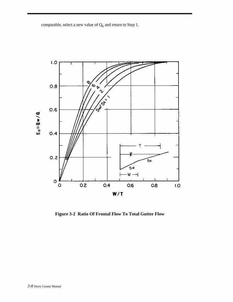
comparable, select a new value of Qs and return to Step 1.
Figure 3-2 Ratio Of Frontal Flow To Total Gutter Flow
3-8 Horry County Manual
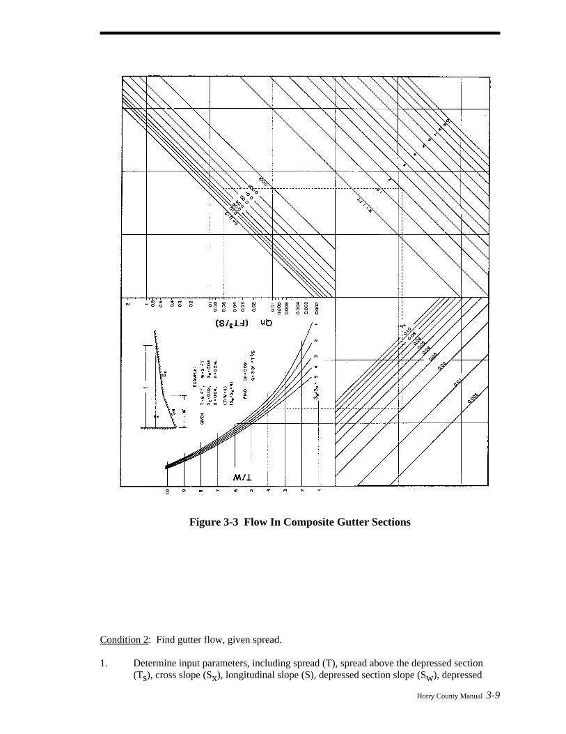
Figure 3-3 Flow In Composite Gutter Sections Condition 2: Find gutter flow, given spread. 1. Determine input parameters, including spread (T), spread above the depressed section
(Ts), cross slope (Sx), longitudinal slope (S), depressed section slope (Sw), depressed
Horry County Manual 3-9

3-10 Horry County Manual
section width (W), Manning's n, and depth of gutter flow (d). 2. Use Figure 3-1 to determine the capacity of the gutter section above the depressed section
(Qs). Use the procedure for uniform cross slopes (Condition 2), substituting Ts for T. 3. Calculate the ratios W/T and Sw/Sx, and, from Figure 3-2, find the appropriate value of
Eo (the ratio of Qw/Q). 4. Calculate the total gutter flow using the equation: Q = Qs / (1 - Eo) (3.3) Where: Q = gutter flow rate (cfs) Qs = flow capacity of the gutter section above the depressed section (cfs) Eo = ratio of frontal flow to total gutter flow (Qw/Q) 5. Calculate the gutter flow in width (W), using Equation 3.2. 3.3.6 Examples Example 1
Given: T = 8 ft Sx = 0.025 ft/ft n = 0.015 S = 0.01 ft/ft Find: (1) Flow in gutter at design spread (2) Flow in width (W = 2 ft) adjacent to the curb Solution: (1) From Figure 3-1, Qn = 0.03 Q = Qn/n = 0.03/0.015 = 2.0 cfs (2) T = 8 - 2 = 6 ft
(Qn)2 = 0.014 (Figure 3-1) (flow in 6 ft width outside of width W) Q = 0.014/0.015 = 0.9 cfs Qw = 2.0 - 0.9 = 1.1 cfs
Flow in the first 2 ft adjacent to the curb is 1.1 cfs and 0.9 cfs in the remainder of the gutter. Example 2 Given: T = 6 ft Sw = 0.0833 ft/ft Ts = 6 - 1.5 = 4.5 ft W = 1.5 ft Sx = 0.03 ft/ft n = 0.014 S = 0.04 ft/ft
Horry County Manual 3-11
Find: Flow in the composite gutter
Solution: (1) Use Figure 3-1 to find the gutter section capacity above the depressed section.
Qsn = 0.018 Qs = 0.018/0.014 = 1.3 cfs (2) Calculate W/T = 1.5/6 = 0.25 and Sw/Sx = 0.0833/0.03 = 2.78
Use Figure 3-2 to find Eo = 0.64 (3) Calculate the gutter flow using Equation 3.3
Q = 1.3/(1 - 0.64) = 3.6 cfs (4) Calculate the gutter flow in width, W, using Equation 3.2
Qw = 3.6 - 1.3 = 2.3 cfs 3.4 Grate Inlets Design 3.4.1 Types Inlets are drainage structures utilized to collect surface water through grate or curb openings and convey it to storm drains or direct outlet to culverts. Grate inlets subject to traffic should be bicycle safe and be load bearing adequate. Appropriate frames should be provided. Inlets used for the drainage of highway surfaces can be divided into three major classes: 1. Grate Inlets - These inlets include grate inlets consisting of an opening in the gutter
covered by one or more grates, and slotted inlets consisting of a pipe cut along the longitudinal axis with a grate of spacer bare to form slot openings.
2. Curb-Opening Inlets - These inlets are vertical openings in the curb covered by a top slab. 3. Combination Inlets - These inlets usually consist of both a curb-opening inlet and a grate
inlet placed in a side-by-side configuration, but the curb opening may be located in part upstream of the grate.
In addition, where significant ponding can occur, in locations such as underpasses and in sag vertical curves in depressed sections, it is good engineering practice to place flanking inlets on each side of the inlet at the low point in the sag. The flanking inlets should be placed so that they will limit spread on low gradient approaches to the level point and act in relief of the inlet at the low point if it should become clogged or if the design spread is exceeded. The design of grate inlets will be discussed in this section, curb inlet design in Section 3.5, and combination inlets in Section 3.6. 3.4.2 Grate Inlets On Grade The capacity of an inlet depends upon its geometry and the cross slope, longitudinal slope, total gutter flow, depth of flow and pavement roughness. The depth of water next to the curb is the major factor in the interception capacity of both gutter inlets and curb opening inlets. At low velocities, all of the water flowing in the section of gutter occupied by the grate, called frontal
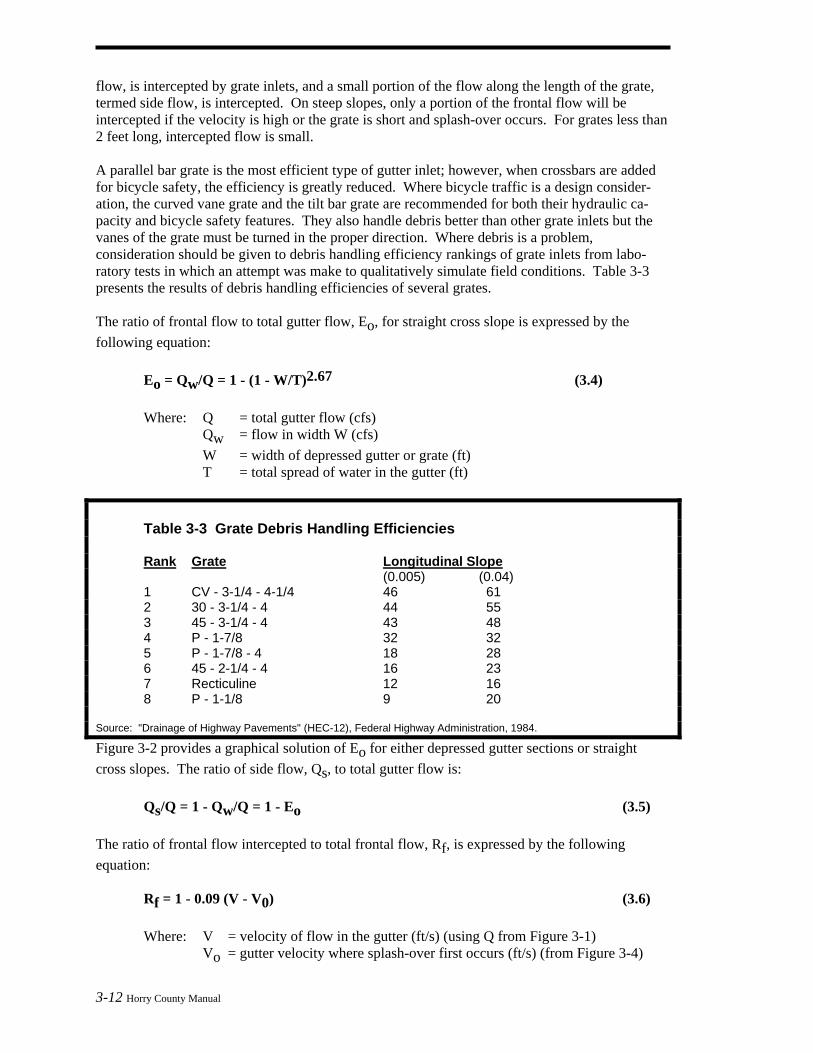
3-12 Horry County Manual
flow, is intercepted by grate inlets, and a small portion of the flow along the length of the grate, termed side flow, is intercepted. On steep slopes, only a portion of the frontal flow will be intercepted if the velocity is high or the grate is short and splash-over occurs. For grates less than 2 feet long, intercepted flow is small. A parallel bar grate is the most efficient type of gutter inlet; however, when crossbars are added for bicycle safety, the efficiency is greatly reduced. Where bicycle traffic is a design consider-ation, the curved vane grate and the tilt bar grate are recommended for both their hydraulic ca-pacity and bicycle safety features. They also handle debris better than other grate inlets but the vanes of the grate must be turned in the proper direction. Where debris is a problem, consideration should be given to debris handling efficiency rankings of grate inlets from labo-ratory tests in which an attempt was make to qualitatively simulate field conditions. Table 3-3 presents the results of debris handling efficiencies of several grates. The ratio of frontal flow to total gutter flow, Eo, for straight cross slope is expressed by the following equation: Eo = Qw/Q = 1 - (1 - W/T)2.67 (3.4) Where: Q = total gutter flow (cfs) Qw = flow in width W (cfs) W = width of depressed gutter or grate (ft) T = total spread of water in the gutter (ft) Table 3-3 Grate Debris Handling Efficiencies Rank Grate Longitudinal Slope (0.005) (0.04) 1 CV - 3-1/4 - 4-1/4 46 61 2 30 - 3-1/4 - 4 44 55 3 45 - 3-1/4 - 4 43 48 4 P - 1-7/8 32 32 5 P - 1-7/8 - 4 18 28 6 45 - 2-1/4 - 4 16 23 7 Recticuline 12 16 8 P - 1-1/8 9 20 Source: "Drainage of Highway Pavements" (HEC-12), Federal Highway Administration, 1984.
Figure 3-2 provides a graphical solution of Eo for either depressed gutter sections or straight cross slopes. The ratio of side flow, Qs, to total gutter flow is: Qs/Q = 1 - Qw/Q = 1 - Eo (3.5) The ratio of frontal flow intercepted to total frontal flow, Rf, is expressed by the following equation: Rf = 1 - 0.09 (V - V0) (3.6) Where: V = velocity of flow in the gutter (ft/s) (using Q from Figure 3-1) Vo = gutter velocity where splash-over first occurs (ft/s) (from Figure 3-4)
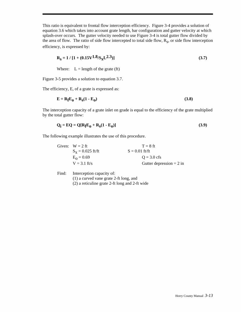
Horry County Manual 3-13
This ratio is equivalent to frontal flow interception efficiency. Figure 3-4 provides a solution of equation 3.6 which takes into account grate length, bar configuration and gutter velocity at which splash-over occurs. The gutter velocity needed to use Figure 3-4 is total gutter flow divided by the area of flow. The ratio of side flow intercepted to total side flow, Rs, or side flow interception efficiency, is expressed by: Rs = 1 / [1 + (0.15V1.8/SxL2.3)] (3.7) Where: L = length of the grate (ft) Figure 3-5 provides a solution to equation 3.7. The efficiency, E, of a grate is expressed as: E = RfEo + Rs(1 - Eo) (3.8) The interception capacity of a grate inlet on grade is equal to the efficiency of the grate multiplied by the total gutter flow: Qi = EQ = Q[RfEo + Rs(1 - Eo)] (3.9) The following example illustrates the use of this procedure. Given: W = 2 ft T = 8 ft Sx = 0.025 ft/ft S = 0.01 ft/ft Eo = 0.69 Q = 3.0 cfs V = 3.1 ft/s Gutter depression = 2 in Find: Interception capacity of:
(1) a curved vane grate 2-ft long, and (2) a reticuline grate 2-ft long and 2-ft wide
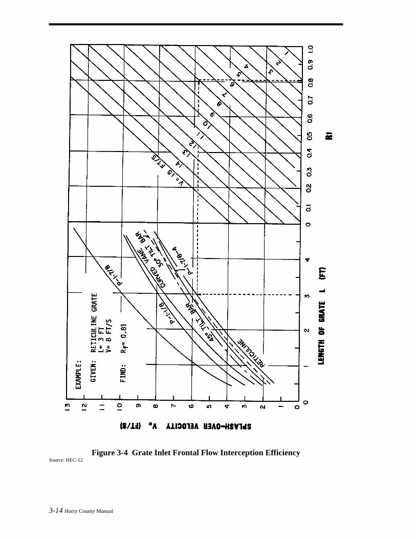
Figure 3-4 Grate Inlet Frontal Flow Interception Efficiency Source: HEC-12
3-14 Horry County Manual
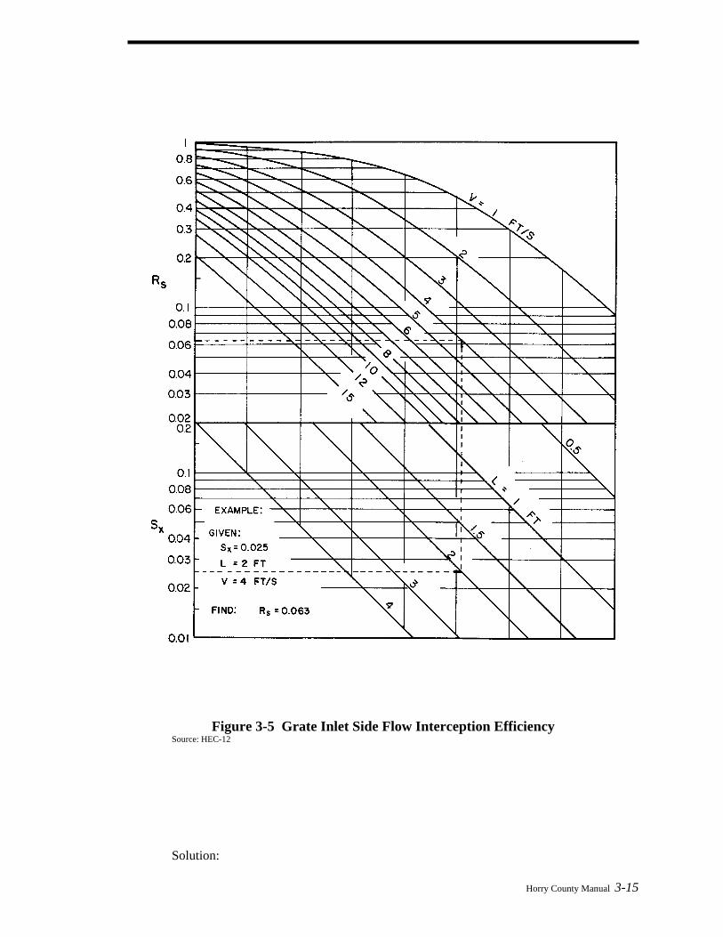
Figure 3-5 Grate Inlet Side Flow Interception Efficiency Source: HEC-12 Solution:
Horry County Manual 3-15

3-16 Horry County Manual
From Figure 3-4 for Curved Vane Grate, Rf = 1.0 From Figure 3-4 for Reticuline Grate, Rf = 1.0 From Figure 3-5 Rs = 0.1 for both grates.
From Equation 3.9: Qi = 3.0[(1.0 X 0.69) + 0.1(1 - 0.69)] = 2.2 cfs For this example the interception capacity of a curved vane grate is the same as that for a reticuline grate for the sited conditions. 3.4.3 Grate Inlets In Sag A grate inlet in a sag operates as a weir up to a certain depth dependent on the bar configuration and size of the grate and as an orifice at greater depths. For standard gutter inlet grate, weir operation continues to a depth of about 0.4 foot above the top of grate and when depth of water exceeds about 1.4 feet, the grate begins to operate as an orifice. Between depths of about 0.4 foot and about 1.4 feet, a transition from weir to orifice flow occurs. The capacity of grate inlets operating as a weir is: Qi = CPd1.5 (3.10) Where: C = 3.0 weir coefficient P = perimeter of grate excluding bar widths and side against the curb (ft) d = depth of water above grate (ft) and as an orifice is: Qi = CA(2gd)0.5 (3.11) Where: C = 0.67 orifice coefficient A = clear opening area of the grate (ft2) g = 32.2 ft/s2 Figure 3-6 is a plot of equations 3.10 and 3.11 for various grate sizes. The effects of grate size on the depth at which a grate operates as an orifice is apparent from the chart. Transition from weir to orifice flow results in interception capacity less than that computed by either weir or the orifice equation. This capacity can be approximated by drawing in a curve between the lines represent-ing the perimeter and net area of the grate to be used.
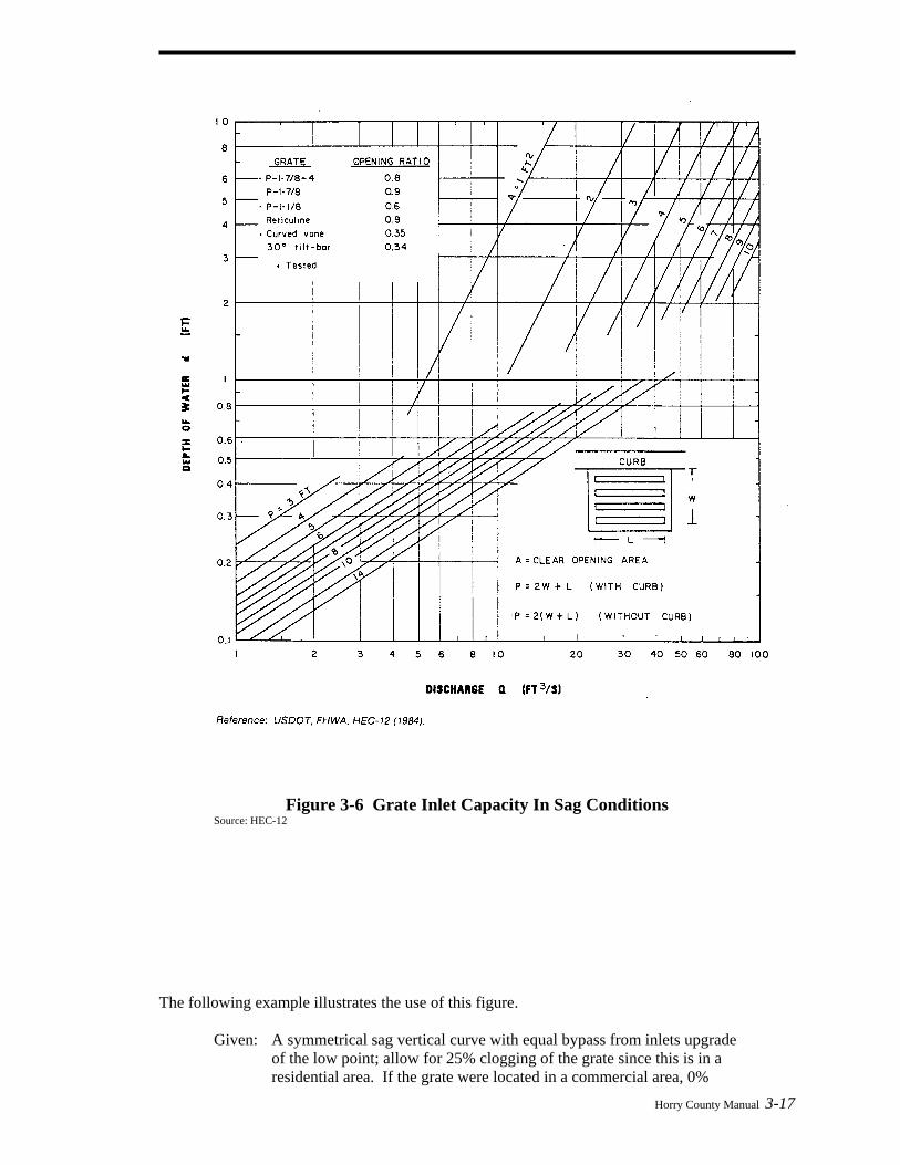
Figure 3-6 Grate Inlet Capacity In Sag Conditions Source: HEC-12 The following example illustrates the use of this figure.
Given: A symmetrical sag vertical curve with equal bypass from inlets upgrade of the low point; allow for 25% clogging of the grate since this is in a residential area. If the grate were located in a commercial area, 0%
Horry County Manual 3-17

3-18 Horry County Manual
clogging could be assumed.
Qb = 3.6 cfs Q = 8 cfs, 25-year storm T = 10 ft, design Sx = 0.05 ft/ft d = TSx = 0.5 ft
Find: Grate size for design Q. Check spread at S = 0.003 ft/ft on approaches to the
low point. Solution: From Figure 3-6, a grate must have a perimeter of 8 ft to intercept 8 cfs at a
depth of 0.5 ft.
Some assumptions must be made regarding the nature of the clogging in order to com-pute the capacity of a partially clogged grate. If the area of a grate is 25 percent covered by debris so that the debris-covered portion does not contribute to interception, the effective perimeter will be reduced by a lesser amount than 25 percent. For example if a 2-ft x 4-ft grate is clogged so that the effective width is 1.5-ft, then the perimeter, P = 1.5 + 4 + 1.5 = 7 ft, rather than 8 ft, the total perimeter, or 6 ft, three-quarters of the total perimeter. The area of the opening would be reduced by 25 percent and the perimeter by 12.5 percent.
Therefore, assuming 25 percent clogging along the length of the grate, a 3 x 4 or a 2 x 5 grate would meet requirements of an 8-ft perimeter 25 percent clogged. Assuming that the installation chosen to meet design conditions is a 2 x 5 ft grate, for 25 percent clogged conditions: P = 1.5 + 5 + 1.5 = 8 ft For 25-year flow: d = 0.5 ft (from Figure 3-6) The American Society of State Highway and Transportation Officials (AASHTO) geo-metric policy recommends a gradient of 0.3 percent within 50 ft of the level point in a sag vertical curve. Check T at S = 0.003 ft/ft for the design flow: Q = 3.6 ft3/s, T = 8.2 ft (25-year storm) (Figure 3-1) Thus, a 2 x 5-ft grate 25 percent clogged is adequate to intercept the design flow at a spread which does not exceed design spread and spread on the approaches to the low point will not exceed design spread. However, the tendency of grate inlets to clog completely warrants consideration of a combination inlet, or curb-opening inlet in a sag where ponding can occur, and flanking inlets on the low gradient approaches.
3.5 Curb Inlet Design 3.5.1 Curb Inlets On Grade Following is a discussion of the procedures for the design of curb inlets on grade. Curb-opening inlets are effective in the drainage of highway pavements where flow depth at the curb is sufficient for the inlet to perform efficiently. Curb openings are relatively free of clogging

Horry County Manual 3-19
tendencies and offer little interference to traffic operation. They are a viable alternative to grates in many locations where grates would be in traffic lanes or would be hazardous for pedestrians or bicyclists. The length of curb-opening inlet required for total interception of gutter flow on a pavement section with a straight cross slope, is determined using Figure 3-7. The efficiency of curb-opening inlets shorter than the length required for total interception, is determined using Figure 3-8. The length of inlet required for total interception by depressed curb-opening inlets or curb-open-ings in depressed gutter sections can be found by the use of an equivalent cross slope, Se, in the following equation. Se = Sx + S'wEo (3.12) Where: Sx = (a/12W) a = gutter depression (in.) W = width of depression for curb opening inlet (ft) S'w= cross slope of the gutter measured from the cross slope of the pavement Eo = ratio of flow in the depressed section to total gutter flow It is apparent from examination of Figure 3-7 that the length of curb opening required for total interception can be significantly reduced by increasing the cross slope or the equivalent cross slope. The equivalent cross slope can be increased by use of a continuously depressed gutter section or a locally depressed gutter section. 3.5.1.1 Design Steps Steps for using Figures 3-7 and 3-8 in the design of curb inlets on grade are given below: (1) Determine the following input parameters: Cross slope = Sx (ft/ft) Longitudinal slope = S (ft/ft) Gutter flow rate = Q (cfs) Manning's n = n Spread of water on pavement = T (ft) from Figure 3-1 (2) Enter Figure 3-7 using the two vertical lines on the left side labeled n and S. Locate the
value for Manning's n and longitudinal slope and draw a line connecting these points and extend this line to the first turning line.
(3) Locate the value for the cross slope (or equivalent cross slope) and draw a line from the
point on the first turning line through the cross slope value and extend this line to the second turning line.
(4) Using the far right vertical line labeled Q locate the gutter flow rate. Draw a line from
this value to the point on the second turning line. Read the length required from the verti-cal line labeled LT.
(5) If the curb-opening inlet is shorter than the value obtained in step 4, Figure 3-8 can be
used to calculate the efficiency. Enter the x-axis with the L/LT ratio and draw a vertical line upward to the E curve. From the point of intersection, draw a line horizontally to the intersection with the y-axis and read the efficiency value.
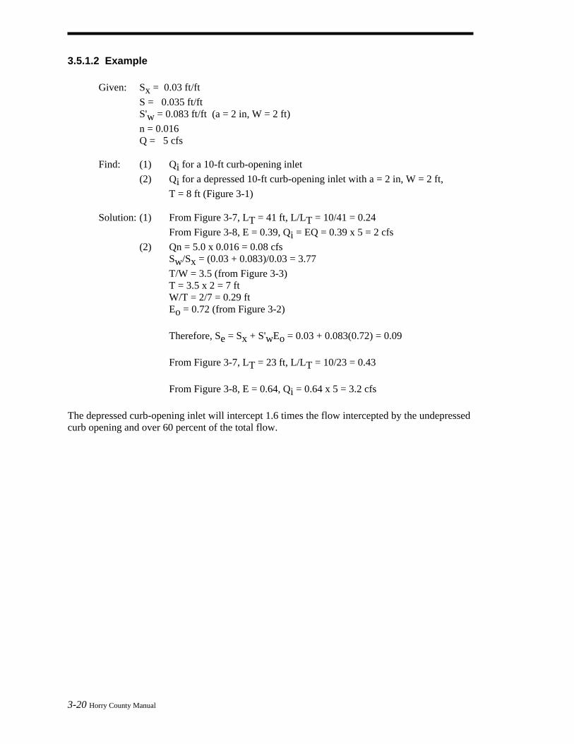
3-20 Horry County Manual
3.5.1.2 Example Given: Sx = 0.03 ft/ft S = 0.035 ft/ft S'w = 0.083 ft/ft (a = 2 in, W = 2 ft) n = 0.016 Q = 5 cfs Find: (1) Qi for a 10-ft curb-opening inlet
(2) Qi for a depressed 10-ft curb-opening inlet with a = 2 in, W = 2 ft, T = 8 ft (Figure 3-1)
Solution: (1) From Figure 3-7, LT = 41 ft, L/LT = 10/41 = 0.24 From Figure 3-8, E = 0.39, Qi = EQ = 0.39 x 5 = 2 cfs (2) Qn = 5.0 x 0.016 = 0.08 cfs Sw/Sx = (0.03 + 0.083)/0.03 = 3.77 T/W = 3.5 (from Figure 3-3) T = 3.5 x 2 = 7 ft W/T = 2/7 = 0.29 ft Eo = 0.72 (from Figure 3-2) Therefore, Se = Sx + S'wEo = 0.03 + 0.083(0.72) = 0.09 From Figure 3-7, LT = 23 ft, L/LT = 10/23 = 0.43 From Figure 3-8, E = 0.64, Qi = 0.64 x 5 = 3.2 cfs The depressed curb-opening inlet will intercept 1.6 times the flow intercepted by the undepressed curb opening and over 60 percent of the total flow.
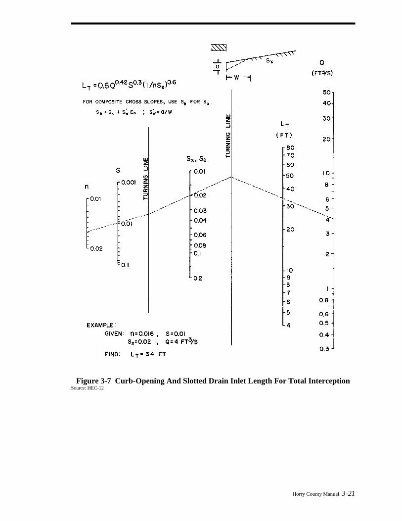
Figure 3-7 Curb-Opening And Slotted Drain Inlet Length For Total Interception Source: HEC-12
Horry County Manual 3-21
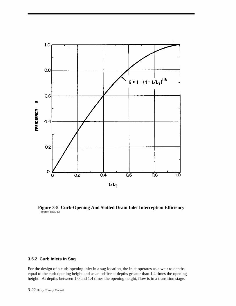
Figure 3-8 Curb-Opening And Slotted Drain Inlet Interception Efficiency Source: HEC-12 3.5.2 Curb Inlets In Sag For the design of a curb-opening inlet in a sag location, the inlet operates as a weir to depths equal to the curb opening height and as an orifice at depths greater than 1.4 times the opening height. At depths between 1.0 and 1.4 times the opening height, flow is in a transition stage. 3-22 Horry County Manual

Horry County Manual 3-23
The capacity of curb-opening inlets in a sag location can be determined from Figure 3-9 which accounts for the operation of the inlet as a weir and as an orifice at depths greater than 1.4h. This figure is applicable to depressed curb-opening inlets and the depth at the inlet includes any gutter depression. The height (h) in the figure assumes a vertical orifice opening (see sketch on Figure 3-9). The weir portion of Figure 3-9 is valid for a depressed curb-opening inlet when d < (h + a/12). The capacity of curb-opening inlets in a sag location with a vertical orifice opening but without any depression can be determined from Figure 3-10. The capacity of curb-opening inlets in a sag location with other than vertical orifice openings can be determined by using Figure 3-11.
3.5.2.1 Design Steps Steps for using Figures 3-9, 3-10, and 3-11 in the design of curb-opening inlets in sag locations are given below:
(1) Determine the following input parameters: Cross slope = Sx (ft/ft) Spread of water on pavement = T (ft) from Figure 3-1
Gutter flow rate = Q (cfs) or dimensions of curb-opening inlet [L (ft) and H (in)] Dimensions of depression if any [a (in) and W (ft)]
(2) To determine discharge given the other input parameters, select the appropriate Figure (3-
9, 3-10, or 3-11 depending whether the inlet is in a depression and if the orifice opening is vertical).
(3) To determine the discharge (Q), given the water depth (d) locate the water depth value on
the y-axis and draw a horizontal line to the appropriate perimeter (p), height (h), length (L), or width x length (hL) line. At this intersection draw a vertical line down to the x-axis and read the discharge value.
(4) To determine the water depth given the discharge, use the procedure described in step 3
except you enter the figure at the value for the discharge on the x-axis.
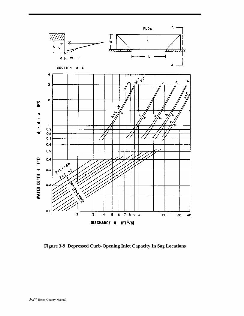
Figure 3-9 Depressed Curb-Opening Inlet Capacity In Sag Locations
3-24 Horry County Manual
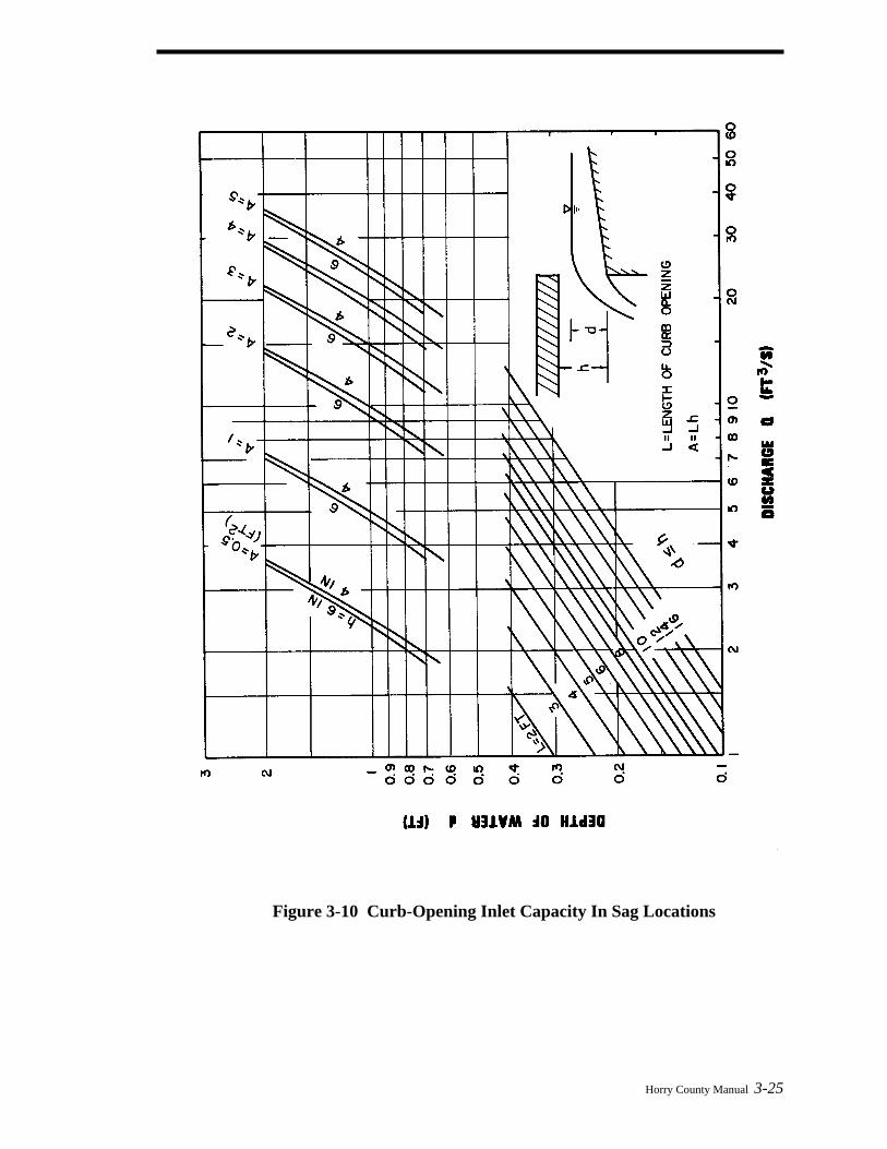
Figure 3-10 Curb-Opening Inlet Capacity In Sag Locations
Horry County Manual 3-25
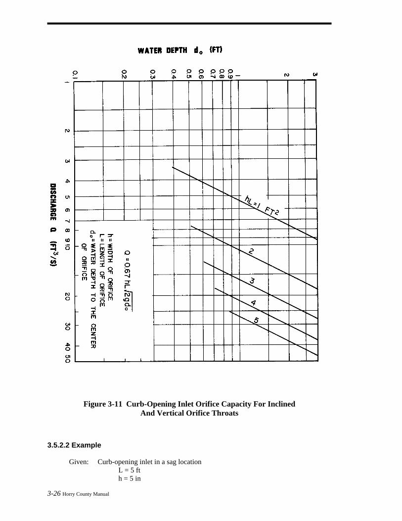
Figure 3-11 Curb-Opening Inlet Orifice Capacity For Inclined And Vertical Orifice Throats
3.5.2.2 Example Given: Curb-opening inlet in a sag location L = 5 ft h = 5 in
3-26 Horry County Manual
Horry County Manual 3-27
(1) Undepressed curb opening Sx = 0.05 ft/ft T = 8 ft (2) Depressed curb opening Sx = 0.05 ft/ft a = 2 in W = 2 ft T = 8 ft Find: Discharge Qi Solution: (1) d = TSx = 8 x 0.05 = 0.4 ft d < h From Figure 3-10, Qi = 3.8 cfs (2) d = 0.4 ft h + a/12 = (5 + 2/12)/12 = 0.43 ft
since d < 0.43, the weir portion of Figure 3-9 is applicable (lower portion of the Figure)
P = L + 1.8W = 5 + 3.6 = 8.6 ft From Figure 3-9, Qi = 5 cfs
At d = 0.4 ft, the depressed curb-opening inlet has about 30 percent more capacity than an inlet without depression. 3.6 Combination Inlets 3.6.1 On Grade On a continuous grade, the capacity of an unclogged combination inlet with the curb opening located adjacent to the grate is approximately equal to the capacity of the grate inlet alone. Thus, capacity is computed by neglecting the curb opening inlet and the design procedures should be followed based on the use of Figures 3-4, 3-5 and 3-6. 3.6.2 In Sag All debris carried by stormwater runoff that is not intercepted by upstream inlets will be con-centrated at the inlet located at the low point, or sag. Because this will increase the probability of clogging for grated inlets, it is generally appropriate to estimate the capacity of a combination inlet at a sag by neglecting the grate inlet capacity. Assuming complete clogging of the grate, Figures 3-9, 3-10, and 3-11 for curb-opening inlets should be used for design. 3.7 Storm Drains 3.7.1 Introduction After the tentative locations of inlets, drain pipes, and outfalls with tail-waters have been deter-mined and the inlets sized, the next logical step is the computation of the rate of discharge to be carried by each drain pipe and the determination of the size and gradient of pipe required to care

3-28 Horry County Manual
for this discharge. This is done by proceeding in steps from upstream of a line to downstream to the point at which the line connects with other lines or the outfall, whichever is applicable. The discharge for a run is calculated, the drainpipe serving that discharge is sized, and the process is repeated for the next run downstream. It should be recognized that the rate of discharge to be carried by any particular section of drain pipe is not necessarily the sum of the inlet design discharge rates of all inlets above that section of pipe, but as a general rule is somewhat less than this total. It is useful to understand that the time of concentration is most influential and as the time of concentration grows larger, the proper rainfall intensity to be used in the design grows smaller. For ordinary conditions, drainpipes should be sized on the assumption that they will flow full or practically full under the design discharge. The Manning Formula is recommended for capacity calculations. 3.7.2 Design Criteria The standard recommended maximum and minimum slopes for storm drains should conform to the following criteria: 1. The maximum hydraulic gradient should not produce a velocity that exceeds 15 feet per
second. 2. The minimum desirable physical slope should be 0.5 percent or the slope which will pro-
duce a velocity of 2 feet per second when the storm sewer is flowing full, whichever is greater.
If the Hydraulic Grade Line elevation exceeds the gutter invert or grate elevation for the design flow, adjustments are needed in the system to reduce the elevation of the hydraulic grade line. Profiles showing the HGL shall be provided for all piped drainage systems. 3.7.3 Capacity Formulas for Gravity and Pressure Flow The most widely used formula for determining the hydraulic capacity of storm drain pipes for gravity and pressure flows is the Manning Formula and it is expressed by the following equation: V = [1.486 R2/3S1/2]/n (3.13) Where: V = mean velocity of flow (ft/s) R = the hydraulic radius (ft) - defined as the area of flow divided by the wet-
ted flow surface or wetted perimeter (A/WP) S = the slope of hydraulic grade line (ft/ft) n = Manning's roughness coefficient In terms of discharge, the above formula becomes: Q = [1.486 AR2/3S1/2]/n (3.14) Where: Q = rate of flow (cfs) A = cross sectional area of flow (ft2) For pipes flowing full, the above equations become: V = [0.590 D2/3S1/2]/n (3.15)

Horry County Manual 3-29
Q = [0.463 D8/3S1/2]/n (3.16) Where: D = diameter of pipe (ft) The Manning's equation can be written to determine friction losses for storm drainpipes as: Hf = [2.87 n2V2L]/[S4/3] (3.17)
Hf = [29 n2V2L]/[(R4/3)(2g)] (3.18) Where: Hf = total head loss due to friction (ft) n = Manning's roughness coefficient D = diameter of pipe (ft) L = length of pipe (ft) V = mean velocity (ft/s) R = hydraulic radius (ft) g = acceleration of gravity = 32.2 ft/sec2 3.7.4 Nomographs And Table The nomograph solution of Manning's formula for full flow in circular storm drainpipes is shown on Figures 3-12, 3-13, and 3-14. Figure 3-15 has been provided to solve the Manning's equation for storm drainpipes flowing partially full.
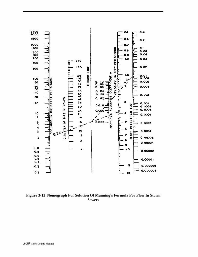
Figure 3-12 Nomograph For Solution Of Manning's Formula For Flow In Storm Sewers
3-30 Horry County Manual
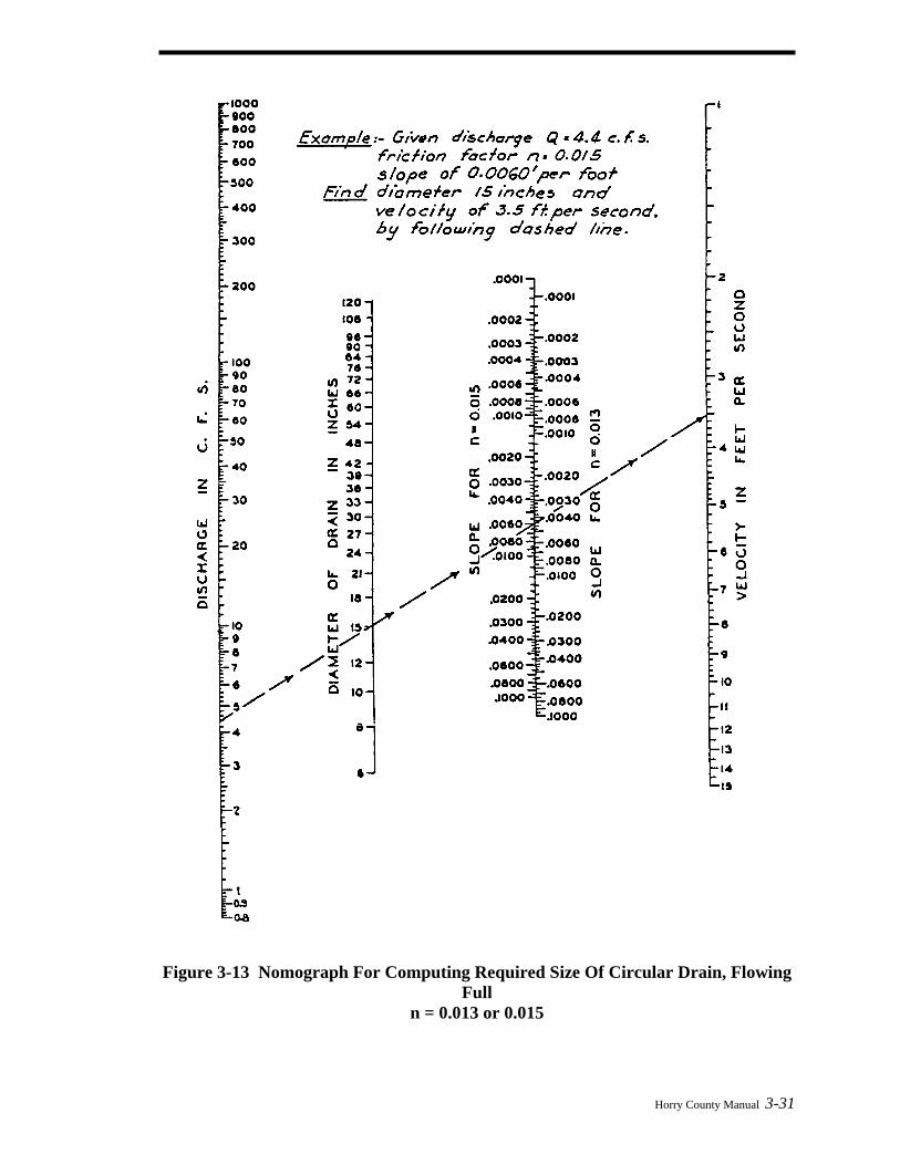
Figure 3-13 Nomograph For Computing Required Size Of Circular Drain, Flowing
Full n = 0.013 or 0.015
Horry County Manual 3-31
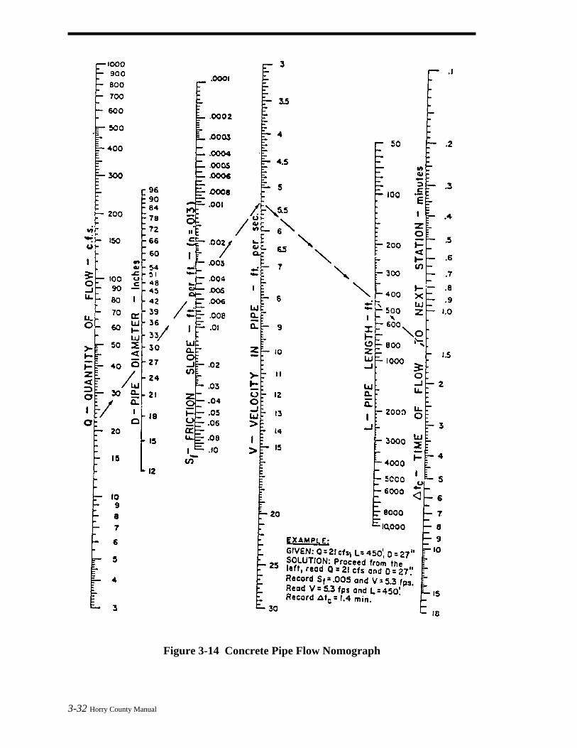
Figure 3-14 Concrete Pipe Flow Nomograph
3-32 Horry County Manual
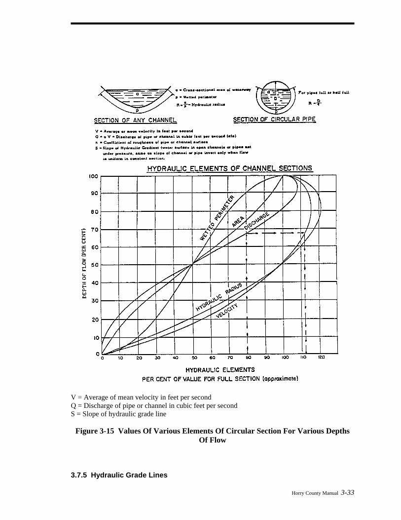
V = Average of mean velocity in feet per second Q = Discharge of pipe or channel in cubic feet per second S = Slope of hydraulic grade line
Figure 3-15 Values Of Various Elements Of Circular Section For Various Depths Of Flow
3.7.5 Hydraulic Grade Lines
Horry County Manual 3-33

3-34 Horry County Manual
All head losses in a storm sewer system are considered in computing the hydraulic grade line (HGL) to determine the water surface elevations, under design conditions in the various inlet, catch basins, manholes, junction boxes, etc. Hydraulic control is a set water surface elevation from which the hydraulic calculations are begun. All hydraulic controls along the alignment are established based on whether the pipe is in inlet or outlet control. If the control is at a main line upstream inlet (inlet control), the hydraulic grade line is the water surface elevation minus the entrance loss minus the difference in velocity head. If the control is at the outlet, the water surface elevation or 0.8 times the pipe diameter (whichever is higher) is the outlet pipe hydraulic grade line. Design Procedure - Outlet Control The head losses are calculated beginning from the control point to the first junction and the procedure is repeated for the next junction. The computation for an outlet control may be tab-ulated using Figure 3-16 using the following procedure: 1. Enter in Col. 1 the station for the junction immediately upstream of the outflow pipe.
Hydraulic grade line computations begin at the outfall and are worked upstream taking each junction into consideration.
2. Enter in Col. 2 the outlet water surface elevation if the outlet will be submerged during the
design storm or 0.8 diameter plus invert out elevation of the outflow pipe whichever is greater.
3. Enter in Col. 3 the diameter (Do) of the outflow pipe. 4. Enter in Col. 4 the design discharge (Qo) for the outflow pipe. 5. Enter in Col. 5 the length (Lo) of the outflow pipe. 6. Enter in Col. 6 the friction slope (Sf) in ft/ft of the outflow pipe. This can be determined
by using the following formula: Sf = (Q2)/K (3.19) Where: Sf = friction slope (ft/ft)
K = [1.486 AR2/3]/n 7. Multiply the friction slope (Sf) in Col. 6 by the length (Lo) in Col. 5 and enter the friction
loss (Hf) in Col. 7. On curved alignments, calculate curve losses by using the formula Hc
= 0.002 (∆)(Vo2/2g), where ∆ = angle of curvature in degrees and add to the friction loss. 8. Enter in col. 8 the velocity of the flow (Vo) of the outflow pipe. 9. Enter in Col. 9 the contraction loss (Ho) by using the formula:
Ho = [0.25 (Vo2)] /2g, where g = 32.2 ft/s2. 10. Enter in Col. 10 the design discharge (Qi) for each pipe flowing into the junction. Neglect
lateral pipes with inflows of less than ten percent of the mainline outflow. Inflow must be
Horry County Manual 3-35
adjusted to the mainline outflow duration time before a comparison is made. 11. Enter in Col. 11 the velocity of flow (Vi) for each pipe flowing into the junction (for
exception see Step 10). 12. Enter in Col. 12 the product of Qi x Vi for each inflowing pipe. When several pipes
inflow into a junction, the line producing the greatest Qi x Vi product is the one that should be used for expansion loss calculations (for exception see Step 10).
13. Enter in Col. 13 the controlling expansion loss (Hi) using the formula:
Hi = [0.35 (Vi2)] /2g. 14. Enter in Col. 14 the angle of skew of each inflowing pipe to the outflow pipe (for excep-
tion, see Step 10). 15. Enter in Col. 15 the greatest bend loss (H∆) calculated by using the formula H∆ = [KVi2)-
]/2g where K = the bend loss coefficient corresponding to the various angles of skew of the inflowing pipes.
16. Enter in Col. 16 the total head loss (Ht) by summing the values in Col. 9 (Ho), Col. 13
(Hi), and Col. 15 (H∆). 17. If the junction incorporates adjusted surface inflow of ten percent or more of the mainline
outflow, i.e., drop inlet, increase Ht by 30 percent and enter the adjusted Ht in Col. 17. 18. If the junction incorporates full diameter inlet shaping, such as standard manholes, reduce
the value of Ht by 50 percent and enter the adjusted value in Col. 18. 19. Enter in Col. 19 the FINAL H, the sum of Hf (Col. 7) and Ht, where Ht is the final ad-
justed value of the Ht. 20. Enter in Col. 20 the sum of the elevation in Col. 2 and the Final H in Col. 19. This eleva-
tion is the potential water surface elevation for the junction under design conditions. 21. Enter in Col. 21 the rim elevation or the gutter invert, whichever is lowest, of the
junction under consideration in Col. 20. If the hydraulic grade line elevation ex-ceeds the gutter invert or grate elevation for the design flow, adjustments are needed in the system to reduce the elevation of the Hydraulic Grade Line (HGL).
22. Repeat the procedure starting with Step 1 for the next junction upstream. 23. At last upstream entrance, add V12/2g to get upstream water surface elevation. 3.7.6 Minimum Grade All storm drains should be designed such that velocities of flow will not be less than 2.0 feet per second at design flow or lower, with a minimum slope of 0.5 percent. For very flat flow lines the general practice is to design components so that flow velocities will increase progressively throughout the length of the pipe system. Upper reaches of a storm drain system should have flatter slopes than slopes of lower reaches. Progressively increasing slopes keep solids moving

3-36 Horry County Manual
toward the outlet and deters settling of particles due to steadily increasing flow velocities. The minimum slopes are calculated by the modified Manning formula: S = [(nV)2]/[2.208 R4/3] (3.20) Where: S = the slope of the hydraulic grade line (ft/ft) n = Manning’s roughness coefficient V = mean velocity of flow (ft/s)
R = hydraulic radius (ft) - area of flow divided by the wetted flow surface or wetted perimeter (A/WP)
3.7.7 Storm Drain Storage If downstream drainage facilities are undersized for the design flow, an above- or below-ground detention structure may be needed to reduce the possibility of flooding. The required storage volume can be provided by using larger than needed storm drain pipes sizes and restrictors to control the release rates at manholes and/or junction boxes in the storm drain system. The same design criteria for sizing the detention basin is used to determine the storage volume required in the system. 3.7.8 Design Procedures The design of storm drain systems is generally divided into the following operations: 1. The first step is the determination of inlet location and spacing as outlined earlier in this
chapter. 2. The second step is the preparation of a plan layout of the storm sewer drainage system
establishing the following design data: a. Location of storm drains. b. Direction of flow. c. Location of manholes. d. Location of existing utilities such as water, gas, or underground cables. 3. The design of the storm drain system is then accomplished by determining drain-
age areas, computing runoff by rational method, and computing the hydraulic capacity by Manning's equation.
4. The storm drain design computation sheet (Figure 3-17) can be used to summarize the
hydrologic, hydraulic and design computations. 5. Examine all assumptions to determine if any adjustments are needed to the final design.

Horry County Manual 3-37
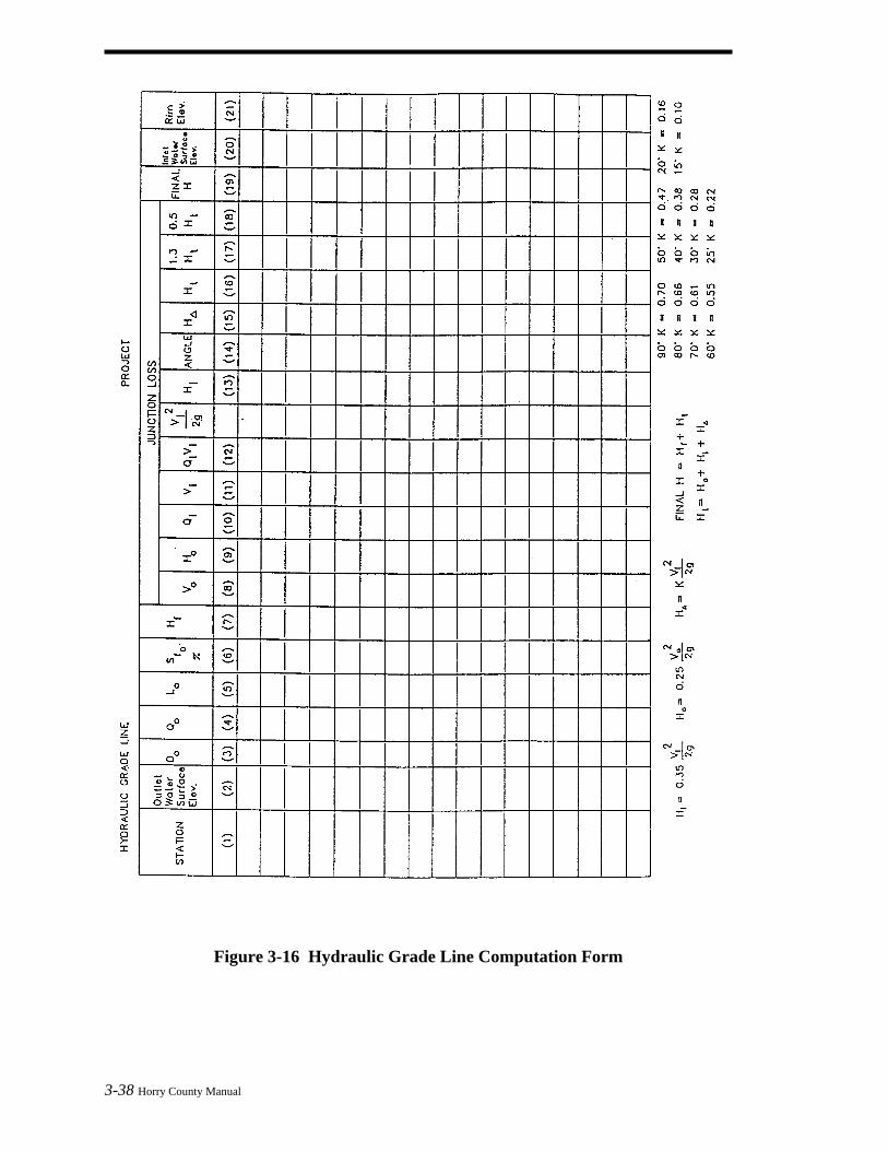
Figure 3-16 Hydraulic Grade Line Computation Form
3-38 Horry County Manual
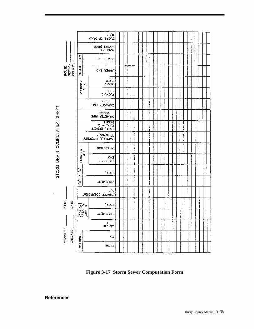
Figure 3-17 Storm Sewer Computation Form References
Horry County Manual 3-39

3-40 Horry County Manual
U. S. Department of Transportation, Federal Highway Administration, 1984. Drainage of Highway Pavements. Hydraulic Engineering Circular No. 12.

Chapter 3 - Storm Drainage Systems 3A-1
DESIGN OF CULVERTS 4
Horry County Manual 4-1
CHAPTER
Chapter Table of Contents 4.1 Introduction............................................................................................................. 4-2 4.2 Symbols And Definitions ........................................................................................ 4-3 4.3 Engineering Design Criteria .................................................................................. 4-3 4.4 Design Procedures................................................................................................... 4-7
4.4.1 Inlet And Outlet Control................................................................................. 4-7 4.4.2 Procedures ...................................................................................................... 4-7 4.4.3 Nomographs.................................................................................................... 4-7 4.4.4 Steps In Design Procedure.............................................................................. 4-8 4.4.5 Performance Curves - Roadway Overtopping.............................................. 4-11 4.4.6 Storage Routing ............................................................................................ 4-13
4.5 Culvert Design Example....................................................................................... 4-14 4.5.1 Introduction .................................................................................................. 4-14 4.5.2 Example ........................................................................................................ 4-14 4.5.3 Example Data ............................................................................................... 4-14 4.5.4 Computations................................................................................................ 4-14
4.6 Design Procedures For Beveled-Edged Inlets .................................................... 4-17 4.6.1 Introduction .................................................................................................. 4-17 4.6.2 Design Figures.............................................................................................. 4-17 4.6.3 Design Procedure.......................................................................................... 4-17 4.6.4 Design Figure Limits .................................................................................... 4-17 4.6.5 Multibarrel Installations ............................................................................... 4-18 4.6.6 Skewed Inlets................................................................................................ 4-18
4.7 Flood Routing And Culvert Design..................................................................... 4-18 4.7.1 Introduction .................................................................................................. 4-18 4.7.2 Design Procedure.......................................................................................... 4-18
4.8 HY8 Culvert Analysis Microcomputer Program............................................... 4-19 References..................................................................................................................... 4-20 Appendix A - Design Charts and Nomographs......................................................... 4-22

4-2 Horry County Manual
This Page Intentionally Left Blank 4.1 Introduction

Horry County Manual 4-3
Primary considerations for the final selection of any drainage structure are that its design be based upon appropriate hydraulic principles, economy, and minimized effects on adjacent property by the resultant headwater depth and outlet velocity. The allowable headwater elevation is that elevation above which damage may be caused to adjacent property and/or the highway. It is this allowable headwater depth that is the primary basis for sizing a culvert. Performance curves should be developed for all culverts for evaluating the hydraulic capacity of a culvert for various headwaters. These will display the consequence of high flow rates at the site and any possible hazards. Sometimes a small increase in flow rate can affect a culvert design. If only the design peak discharge is used in the design, the engineer cannot assess what effect increases in the estimated design discharge will have on the culvert design. 4.2 Symbols And Definitions To provide consistency within this chapter as well as throughout this manual the following symbols will be used. These symbols were selected because of their wide use in many culvert design publications. Table 4-1 Symbols And Definitions Symbol Definition Units A Area of cross section of flow sq ft B Barrel width ft Cd Overtopping discharge coefficient - D Culvert diameter or barrel depth in. or ft d Depth of flow ft dc Critical depth of flow ft du Uniform depth of flow ft
g Acceleration due to gravity (32.2 ft/s2) ft/s2 Hf Depth of pool or head, above the face section of invert ft ho Height of hydraulic grade line above outlet invert ft HW Headwater depth above invert of culvert (depth from inlet invert to upstream total energy grade line) ft Ke Inlet loss coefficient - L Length of culvert ft N Number of barrels - Q Rate of discharge cfs S Slope of culvert ft/ft TW Tailwater depth above invert of culvert ft V Mean velocity of flow ft/s Vc Critical velocity ft/s
4.3 Engineering Design Criteria The design of a culvert should take into account many different engineering and technical aspects

4-4 Horry County Manual
at the culvert site and adjacent areas. The following design criteria should be considered for all culvert designs as applicable. Flood Frequency - The design storm for culverts, except for culverts under arterial roads, is the 25-year storm. For culverts under arterial roads, the 50-year storm shall be used for design. Velocity Limitations - Both minimum and maximum velocities should be considered when designing a culvert. The maximum velocity should be consistent with channel stability requirements at the culvert outlet. Buoyancy Protection - Headwalls, endwalls, slope paving or other means of anchoring to provide buoyancy protection should be considered for all flexible culverts. Length And Slope - The culvert length and slope should be chosen to approximate existing topography, and to the degree practicable: the culvert invert should be aligned with the channel bottom and the skew angle of the stream, and the culvert entrance should match the geometry of the roadway embankment. Debris Control - In designing debris control structures it is recommended that the Hydraulic Engineering Circular No. 9 entitled "Debris Control Structures" be consulted. Headwater Limitations - The allowable headwater elevation is determined from an evaluation of land use upstream of the culvert and the proposed or existing roadway elevation. Headwater is the depth of water above the culvert invert at the entrance end of the culvert. Tailwater Considerations - The hydraulic conditions downstream of the culvert site must be evaluated to determine a tailwater depth for a range of discharge. At times, there may be a need for calculating backwater curves to establish the tailwater conditions. The following conditions must be considered:
• If the culvert outlet is operating with a free outfall, the critical depth and equivalent hydraulic grade line should be determined.
• For culverts, which discharge to an open channel, the stage-discharge curve for the channel must be determined. See Chapter 5 - Open Channel Design.
• If an upstream culvert outlet is located near a downstream culvert inlet, the headwater elevation of the downstream culvert may establish the design tailwater depth for the upstream culvert.
• If the culvert discharges to a lake, pond, or other major water body, the expected high water elevation of the particular water body may establish the culvert tailwater.
Storage - If storage is being assumed upstream of the culvert, consideration should be given to:
• the total area of flooding, and • the average time that bankfull stage is exceeded for the design flood up to 48 hours in
rural areas or 6 hours in urban areas. Culvert Inlets - Hydraulic efficiency and cost can be significantly affected by inlet conditions. The inlet coefficient Ke, is a measure of the hydraulic efficiency of the inlet, with lower values indicating greater efficiency. Recommended inlet coefficients are given in Table 4-2. Inlets With Headwalls - Headwalls may be used for a variety of reasons including increasing the efficiency of the inlet, providing embankment stability, providing embankment protection against erosion, providing protection from buoyancy, and shorten the length of the required structure.
Horry County Manual 4-5
If high headwater depths are to be encountered, or the approach velocity in the channel will cause scour, a short channel apron should be provided at the toe of the headwall. This apron should extend at least one pipe diameter upstream from the entrance, and the top of the apron should not protrude above the normal streambed elevation. Wingwalls And Aprons - Wingwalls are used where the side slopes of the channel adjacent to the entrance are unstable or where the culvert is skewed to the normal channel flow. Improved Inlets - Where inlet conditions control the amount of flow that can pass through the culvert, improved inlets can greatly increase the hydraulic performance at the culvert. Material Selection - Reinforced concrete pipe (RCP) is recommended for use (1) under a roadway, or (2) under driveways within right-of-way. High Density Polyethylene pipe can be used for installations that do not involve traffic bearing applications. Only interior smooth liner High-Density Polyethylene pipe is acceptable. Corrugated High-Density Polyethylene pipe is not acceptable. Table 4-3 gives recommended Manning's n values for different materials. Culvert Skews - Culvert skews shall not exceed 45 degrees as measured from a line perpendicular to the roadway centerline without approval. Culvert Sizes - The minimum allowable pipe diameter shall be 15 inches. Weep Holes - Weep holes are sometimes used to relieve uplift pressure. Filter materials should be used in conjunction with the weep holes in order to intercept the flow and prevent the formation of piping channels. The filter materials should be designed as underdrain filter so that it will not become clogged and so that piping cannot occur through the pervious material and the weep hole. Outlet Protection - Outlet protection should be provided where erosive potential is a design concern. Environmental Considerations - Where compatible with good hydraulic engineering, a site should be selected that will permit the culvert to be constructed to cause the least impact on the stream or wetlands. This selection must consider the entire site, including any necessary lead channels. Table 4-2 Inlet Coefficients Type of Structure and Design of Entrance Coefficient Ke Pipe, Concrete Projecting from fill, socket end (grove-end) 0.2 Projecting from fill, square cut end 0.5 Headwall or headwall and wingwalls Socket end of pipe (groove-end) 0.2
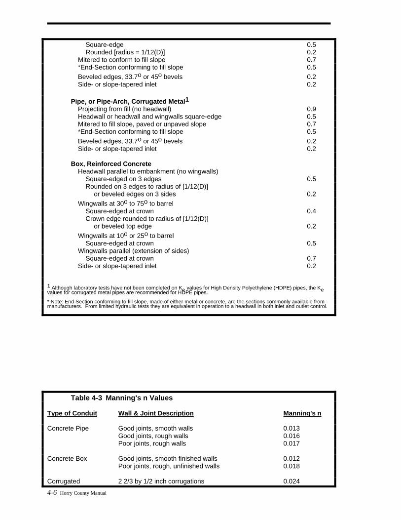
4-6 Horry County Manual
Square-edge 0.5 Rounded [radius = 1/12(D)] 0.2 Mitered to conform to fill slope 0.7 *End-Section conforming to fill slope 0.5 Beveled edges, 33.7o or 45o bevels 0.2 Side- or slope-tapered inlet 0.2 Pipe, or Pipe-Arch, Corrugated Metal1 Projecting from fill (no headwall) 0.9 Headwall or headwall and wingwalls square-edge 0.5 Mitered to fill slope, paved or unpaved slope 0.7 *End-Section conforming to fill slope 0.5 Beveled edges, 33.7o or 45o bevels 0.2 Side- or slope-tapered inlet 0.2 Box, Reinforced Concrete Headwall parallel to embankment (no wingwalls) Square-edged on 3 edges 0.5 Rounded on 3 edges to radius of [1/12(D)] or beveled edges on 3 sides 0.2 Wingwalls at 30o to 75o to barrel Square-edged at crown 0.4 Crown edge rounded to radius of [1/12(D)] or beveled top edge 0.2 Wingwalls at 10o or 25o to barrel Square-edged at crown 0.5 Wingwalls parallel (extension of sides) Square-edged at crown 0.7 Side- or slope-tapered inlet 0.2 1 Although laboratory tests have not been completed on K values for High Density Polyethylene (HDPE) pipes, the Ke evalues for corrugated metal pipes are recommended for HDPE pipes. * Note: End Section conforming to fill slope, made of either metal or concrete, are the sections commonly available from manufacturers. From limited hydraulic tests they are equivalent in operation to a headwall in both inlet and outlet control.
Table 4-3 Manning's n Values Type of Conduit Wall & Joint Description Manning's n Concrete Pipe Good joints, smooth walls 0.013 Good joints, rough walls 0.016 Poor joints, rough walls 0.017 Concrete Box Good joints, smooth finished walls 0.012 Poor joints, rough, unfinished walls 0.018 Corrugated 2 2/3 by 1/2 inch corrugations 0.024
Horry County Manual 4-7
Metal Pipes and 6 by 1 inch corrugations 0.025 Boxes with 5 by 1 inch corrugations 0.026 Annular 3 by 1 inch corrugations 0.028 Corrugations 6 by 2 inch structural plate 0.035 9 by 2 1/2 inch structural plate 0.035 Corrugated Metal 2 2/3 by 1/2 inch corrugated Pipes, Helical 24 inch plate width 0.012 Corrugations, Full Circular Flow Spiral Rib Metal 3/4 by 3/4 in recesses at 12 inch Pipe spacing, good joints 0.013 High Density Corrugated Smooth Liner 0.011 Polyethylene Corrugated Interior 0.024 (HDPE) Polyvinyl Chloride (PVC) 0.011 Note: For further information concerning Manning n values for selected conduits consult Hydraulic Design of Highway
Culverts, Federal Highway Administration, HDS No. 5, page 163
4.4 Design Procedures 4.4.1 Inlet And Outlet Control Inlet Control - If the culvert is operating on a steep slope, it is likely that the entrance geometry will control the headwater and the culvert will be on inlet control. Outlet Control - If the culvert is operating on a mild slope, the outlet characteristics will probably control the flow and the culvert will be on outlet control. Proper culvert design and analysis requires checking for both inlet and outlet control to determine which will govern particular culvert designs. For more information on inlet and outlet control see the Federal Highway Administration publication entitled - Hydraulic Design Of Highway Culverts, HDS-5, 1985, and AASHTO Model Drainage Manual, 1998. 4.4.2 Procedures There are two procedures for designing culverts: (1) the manual use of inlet and outlet control nomographs and (2) the use of a personal computer system such as HY8 - Culvert Analysis Microcomputer Program (see Section 4.8 of this manual). The following will outline the design procedures for use of the nomograph. 4.4.3 Nomographs The use of nomographs require a trial and error solution. The solution is quite easy and provides reliable designs for many applications. It should be remembered that velocity, hydrograph routing, roadway overtopping, and outlet scour require additional, separate computations beyond what can be obtained from the nomographs.
4-8 Horry County Manual
Figures 4-1 and 4-2 show examples of an inlet control and outlet control nomographs that can be used to design concrete pipe culverts. For culvert designs not covered by these nomographs, refer to the complete set of nomographs given in Appendix A at the end of this chapter. 4.4.4 Steps In Design Procedure The design procedure requires the use of inlet and outlet nomographs. Step Action (1) List design data: Q = discharge (cfs) L = culvert length (ft) S = culvert slope (ft/ft) TW= tailwater depth (ft) V = velocity for trial diameter (ft/s) Ke= inlet loss coefficient HW= allowable headwater depth for the design storm (ft) (2) Determine trail culvert size by assuming a trial velocity 3 to 5 ft/s and computing
the culvert area, A = Q/V. Determine the culvert diameter (inches). (3) Find the actual HW for the trial size culvert for both inlet and outlet control.
• For inlet control, enter inlet control nomograph with D and Q and find HW/D for the proper entrance type.
• Compute HW and, if too large or two small, try another culvert size before computing HW for outlet control.
• For outlet control enter the outlet control nomograph with the culvert length, entrance loss coefficient, and trial culvert diameter.
• To compute HW, connect the length scale for the type of entrance condition and culvert diameter scale with a straight line, pivot on the turning line, and draw a straight line from the design discharge through the turning point to the head loss scale H. Compute the headwater elevation HW from the equation:
HW = H + ho - LS (4.1)
Where: ho = ½ (critical depth + D), or tailwater depth, whichever is greater.
(4) Compare the computed headwaters and use the higher HW nomograph to
determine if the culvert is under inlet or outlet control.
If outlet control governs and the HW is unacceptable, select a larger trial size and find another HW with the outlet control nomographs. Since the smaller size of culvert had been selected for allowable HW by the inlet control nomographs, the inlet control for the larger pipe need not be checked.
(5) Calculate exit velocity and expected streambed scour to determine if an energy dissipater is needed.

Horry County Manual 4-9
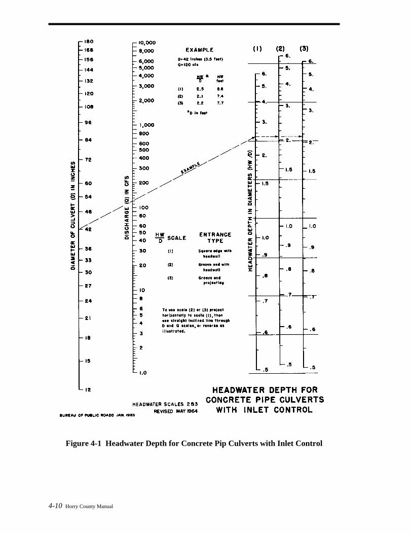
Figure 4-1 Headwater Depth for Concrete Pip Culverts with Inlet Control
4-10 Horry County Manual
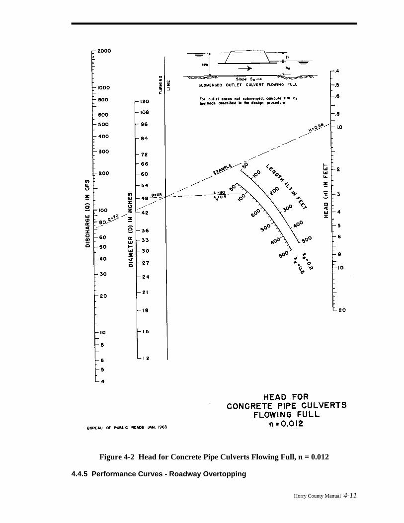
Figure 4-2 Head for Concrete Pipe Culverts Flowing Full, n = 0.012 4.4.5 Performance Curves - Roadway Overtopping
Horry County Manual 4-11
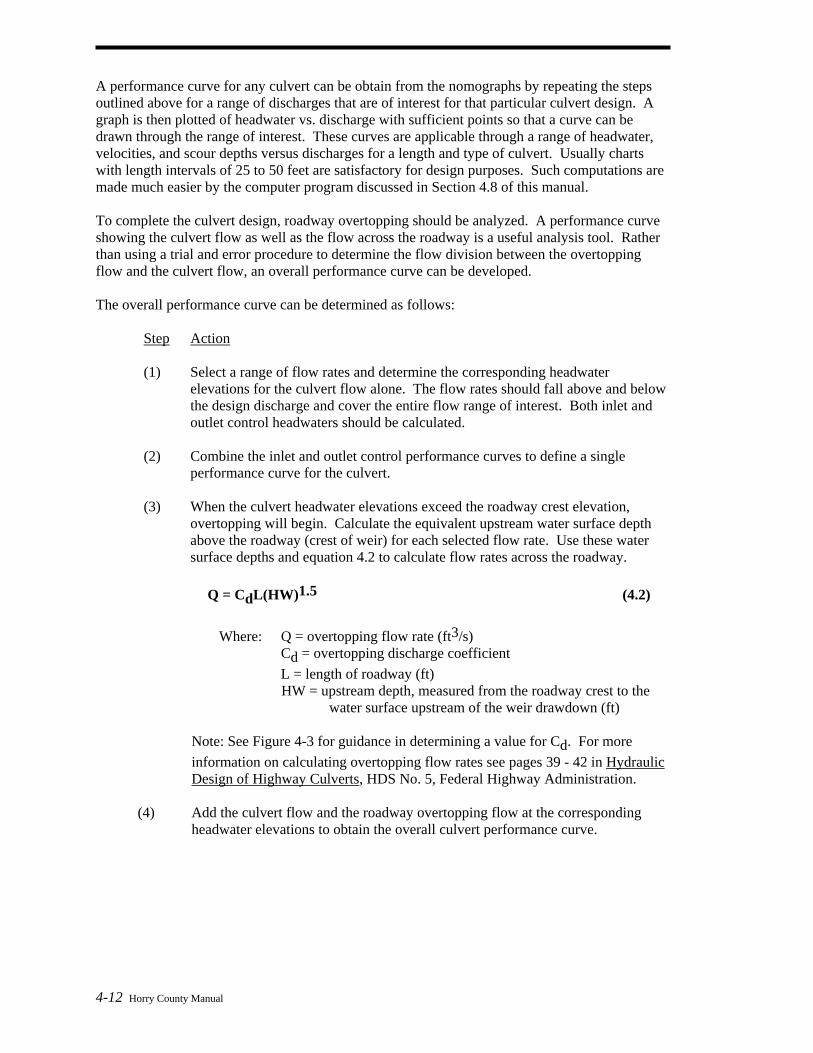
4-12 Horry County Manual
A performance curve for any culvert can be obtain from the nomographs by repeating the steps outlined above for a range of discharges that are of interest for that particular culvert design. A graph is then plotted of headwater vs. discharge with sufficient points so that a curve can be drawn through the range of interest. These curves are applicable through a range of headwater, velocities, and scour depths versus discharges for a length and type of culvert. Usually charts with length intervals of 25 to 50 feet are satisfactory for design purposes. Such computations are made much easier by the computer program discussed in Section 4.8 of this manual. To complete the culvert design, roadway overtopping should be analyzed. A performance curve showing the culvert flow as well as the flow across the roadway is a useful analysis tool. Rather than using a trial and error procedure to determine the flow division between the overtopping flow and the culvert flow, an overall performance curve can be developed. The overall performance curve can be determined as follows: Step Action (1) Select a range of flow rates and determine the corresponding headwater
elevations for the culvert flow alone. The flow rates should fall above and below the design discharge and cover the entire flow range of interest. Both inlet and outlet control headwaters should be calculated.
(2) Combine the inlet and outlet control performance curves to define a single
performance curve for the culvert. (3) When the culvert headwater elevations exceed the roadway crest elevation,
overtopping will begin. Calculate the equivalent upstream water surface depth above the roadway (crest of weir) for each selected flow rate. Use these water surface depths and equation 4.2 to calculate flow rates across the roadway.
Q = CdL(HW)1.5 (4.2) Where: Q = overtopping flow rate (ft3/s) Cd = overtopping discharge coefficient L = length of roadway (ft)
HW = upstream depth, measured from the roadway crest to the water surface upstream of the weir drawdown (ft)
Note: See Figure 4-3 for guidance in determining a value for Cd. For more information on calculating overtopping flow rates see pages 39 - 42 in Hydraulic Design of Highway Culverts, HDS No. 5, Federal Highway Administration.
(4) Add the culvert flow and the roadway overtopping flow at the corresponding
headwater elevations to obtain the overall culvert performance curve.
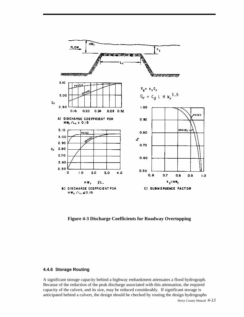
Figure 4-3 Discharge Coefficients for Roadway Overtopping 4.4.6 Storage Routing
Horry County Manual 4-13
A significant storage capacity behind a highway embankment attenuates a flood hydrograph. Because of the reduction of the peak discharge associated with this attenuation, the required capacity of the culvert, and its size, may be reduced considerably. If significant storage is anticipated behind a culvert, the design should be checked by routing the design hydrographs
4-14 Horry County Manual
through the culvert to determine the discharge and stage behind the culvert. Routing procedures are outlined in Hydraulic Design of Highway Culverts, Section V - Storage Routing, HDS No. 5, Federal Highway Administration. 4.5 Culvert Design Example 4.5.1 Introduction The following example problem illustrates the procedures to be used in designing culverts using the nomographs. 4.5.2 Example Size a culvert given the following example data, which were determined by physical limitations at the culvert site and hydraulic procedures, described elsewhere in this manual. 4.5.3 Example Data Input Data Discharge for 50-yr flood = 70 cfs (Note: culvert is located under arterial road) Discharge for 100-yr flood = 176 cfs Allowable Hw for 50-yr discharge = 4.5 ft Allowable Hw for 100-yr discharge = 7.0 ft Length of culvert = 100 ft Natural channel invert elevations: inlet = 15.50 ft, outlet = 15.35 ft Culvert slope = 0.0015 ft/ft Tailwater depth for 50-yr discharge = 3.0 ft Tailwater depth for 100-yr discharge = 4.0 ft
Tailwater depth is the normal depth in downstream channel Entrance type = Groove end with headwall 4.5.4 Computations Steps Computation 1. Assume a culvert velocity of 5 ft/s. Required flow area = (70 cfs)/(5 ft/s) = 14
sq. ft (for the 50-yr recurrence flood). 2. The corresponding culvert diameter is about 48 inches. This can be calculated by
using the formula for area of a circle: Area = (3.14D2)/4 or D = [(Area times 4)/3.14]0.5. Therefore: D = [(14 sq ft x 4)/3.14]0.5 x 12 in./ft) = 50.7 in.
3. A grooved end culvert with a headwall is selected for the design. Using the inlet
control nomograph (Figure 4-1), with a pipe diameter of 48 inches and a discharge of 70 cfs; read a HW/D value of 0.93.
4. The depth of headwater (HW) is (0.93) x (4) = 3.72 ft which is less than the
allowable headwater of 4.5 ft. 5. The culvert is checked for outlet control by using Figure 4-2.

Horry County Manual 4-15
With an entrance loss coefficient Ke of 0.20, a culvert length of 100 ft, and a pipe diameter of 48 inches, an H value of 0.77 ft is determined. The headwater for outlet control is computed by the equation: HW = H + ho - LS For the tailwater depth lower than the top of culvert, ho = Tw or ½ (critical depth in culvert + D) whichever is greater.
ho = 3.0 ft or ho = ½ (2.55 + 4.0) = 3.28 ft
The headwater depth for outlet control is: HW = H + ho - LS = 0.77 + 3.28 - [(100) x (0.0015)] = 3.90 ft
6. Since HW for outlet control (3.90 ft) is greater than the HW for inlet control
(3.72 ft), outlet control governs the culvert design.
Thus, the maximum headwater expected for a 50-yr recurrence flood is 3.90 ft, which is less than the allowable headwater of 4.5 ft.
7. The performance of the culvert is checked for the 100-yr discharge.
The allowable headwater for a 100-yr discharge is 7 ft; critical depth in the 48 inch diameter culvert for the 100-yr discharge is 3.96 ft.
For outlet control, an H value of 5.2 is read from the outlet control nomograph. The maximum headwater is: HW = H + ho - LS = 5.2 + 4.0 - [(100) x (0.0015)] = 9.05 ft.
This depth is greater than the allowable depth of 7ft, thus a larger size culvert must be selected.
8. A 54 inch diameter culvert is tried and found to have a maximum headwater
depth of 3.74 ft. for the 50-yr discharge and of 6.97 ft. for the 100-yr discharge. These values are acceptable for the design conditions.
9. Estimate outlet exit velocity. Since this culvert is under outlet control and
discharges into an open channel downstream, the culvert will be flowing full at the flow depth in the channel. Using the 50-yr design peak discharge of 70 cfs and the area of a 54 inch or 4.5 ft diameter culvert the exit velocity will be: Q = VA Therefore: V = 70 / [3.14(4.0)2]/4 = 4.4 ft/s
10. The design engineer should check minimum velocities for low frequency flows if
the larger storm event (100-yr) controls culvert design. Figure 4-4 provides a convenient form to organize culvert design calculations.
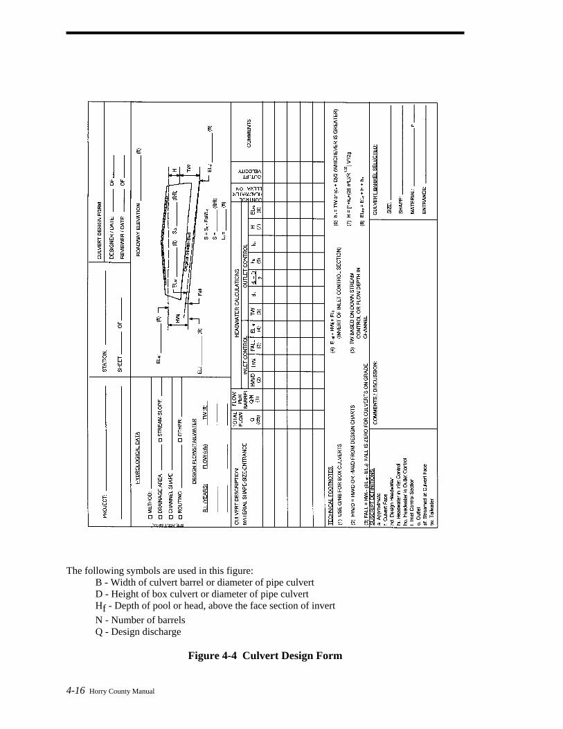
The following symbols are used in this figure: B - Width of culvert barrel or diameter of pipe culvert D - Height of box culvert or diameter of pipe culvert Hf - Depth of pool or head, above the face section of invert N - Number of barrels Q - Design discharge
Figure 4-4 Culvert Design Form
4-16 Horry County Manual

Horry County Manual 4-17
4.6 Design Procedures For Beveled-Edged Inlets 4.6.1 Introduction Improved inlets include inlet geometry refinements beyond those normally used in conventional culvert design practice. Several degrees of improvements are possible, including bevel-edged, side-tapered, and slope-tapered inlets. Those designers interested in using side- and slope-tapered inlets should consult the detailed design criteria and example designs outlined in the U. S. Department of Transportation publication Hydraulic Engineering Circular No. 5 entitled, Hydraulic Design of Highway Culverts, Federal Highway Administration. 4.6.2 Design Figures Four inlet control figures for culverts with beveled edges are included in Appendix A at the end of this chapter. Chart Use for 3 circular pipe culverts with beveled rings 10 90o headwalls (same for 90o wingwalls) 11 skewed headwalls 12 wingwalls with flare angles of 18 to 45 degrees 4.6.3 Design Procedure The figures for bevel-edged inlets are used for design in the same manner as the conventional inlet design nomographs discussed earlier. Note that Charts 10, 11, and 12 apply only to bevels having either a 33o angle (1.5:1) or a 45o angle (1:1). For box culverts, the dimensions of the bevels to be used are based on the culverts dimensions. The top bevel dimension is determined by multiplying the height of the culvert by a factor. The side bevel dimensions are determined by multiplying the width of the culvert by a factor. For a 1:1 bevel, the factor is ½ inch/ft. For a 1.5:1 bevel, the factor is 1 inch/ft. For example the minimum bevel dimensions for a 8 ft x 6 ft box culvert with 1:1 bevels would be:
Top Bevel = d = 6 ft x ½ inch/ft = 3 inches Side Bevel = b = 8 ft x ½ inch/ft = 4 inches
For a 1.5:1 bevel, computations would result in d = 6 and b = 8 inches. 4.6.4 Design Figure Limits The improved inlet design figures are based on research results from culvert models with barrel width, B, to depth, D, ratios of from 0.5:1 to 2:1. For box culverts with more than one barrel, the figures are used in the same manner as for a single barrel, except that the bevels must be sized on the basis of the total clear opening rather than on individual barrel size. For example, in a double 8 ft by 8 ft box culvert:
Top Bevel - is proportioned based on the height of 8 ft which results in a bevel of 4 in. for the 1:1 bevel and 8 in. for the 1.5:1 bevel. Side Bevel - is proportioned based on the clear width of 16 ft which results in a bevel of 8 in. for the 1:1 bevel and 16 in. for the 1.5:1 bevel.
4-18 Horry County Manual
4.6.5 Multibarrel Installations For multibarrel installations exceeding a 3:1 width to depth ratio, the side bevels become excessively large when proportioned on the basis of the total clear width. For these structures, it is recommended that the side bevel be sized in proportion to the total clear width, B, or three times the height, whichever is smaller. The top bevel dimension should always be based on the culvert height. The shape of the upstream edge of the intermediate walls of multibarrel installations is not as important to the hydraulic performance of a culvert as the edge condition of the top and sides. Therefore, the edges of these walls may be square, rounded with a radius of one-half their thickness, chamfered, or beveled. The intermediate walls may also project from the face and slope downward to the channel bottom to help direct debris through the culvert. Multibarrel pipe culverts should be designed as a series of single barrel installations since each pipe requires a separate bevel. 4.6.6 Skewed Inlets It is recommended that Chart 11 in Appendix A for skewed inlets not be used for multiple barrel installations, as the intermediate wall could cause an extreme contraction in the downstream barrels. This would result in under design due to a greatly reduced capacity. Skewed inlets should be avoided whenever possible, and should not be used with side or slope-tapered inlets. It is important to align culverts with streams in order to avoid erosion problems associated with changing the direction of the natural stream flow. 4.7 Flood Routing And Culvert Design 4.7.1 Introduction Flood routing through a culvert is a practice that evaluates the effect of temporary upstream ponding caused by the culvert's backwater. By not considering flood routing, it is possible that the findings from culvert analyses will be conservative. If the selected allowable headwater is considered acceptable without flood routing, then costly over design of both the culvert and outlet protection may result, depending on the amount of temporary storage involved. However, if storage is used in the design of culverts, consideration should be given to:
• the total area of flooding, and • the average time that bankfull stage is exceeded for the design flood up to 48 hours in rural
areas or 6 hours in urban areas. Ignoring temporary storage effects on reducing the selected design flood magnitude by assuming that this provides a factor of safety is not recommended. This practice results in inconsistent factors of safety at culvert sites as it is dependent on the amount of temporary storage at each site. Further, with little or no temporary storage at a site the factor of safety would be unity thereby precluding a factor of safety. If a factor of safety is desired, it is essential that flood routing practices be used to insure consistent and defensible factors of safety are used at all culvert sites. 4.7.2 Design Procedure The design procedure for flood routing through a culvert is the same as for reservoir routing. The site data and roadway geometry are obtained and the hydrology analysis completed to include estimating a hydrograph. Once this essential information is available, the culvert can be
Horry County Manual 4-19
designed. Flood routing through a culvert can be time consuming. It is recommended that the HY8 computer program be used as it contains software that very quickly routes floods through a culvert to evaluate an existing culvert (review), or to select a culvert size that satisfies given criteria (design). However, the engineer should be familiar with the culvert flood routing design process. A multiple trial and error procedure is required for culvert flood routing. In general:
• a trial culvert(s) is selected, • a trial discharge for a particular hydrograph time increment (selected time increment to estimate discharge from the design hydrograph) is selected, • flood routing computations are made with successive trial discharges until the flood routing equation is satisfied, • the hydraulic findings are compared to the selected site criteria, and • if the selected site criteria are satisfied then a trial discharge for the next time increment is
selected and this procedure is repeated; if not, a new trial culvert is selected and the entire procedure is repeated.
4.8 HY8 Culvert Analysis Microcomputer Program It is recommended that the HY8 computer model be used for culvert design. This culvert design model is available in many computer software packages and is included in the HYDRAIN system available from McTrans Software (address given under References below). The personal computer system HYDRAIN uses the theoretical basis for the nomographs to size a culvert. In addition, this system can evaluate improved inlets, generate and route hydrographs, consider road overtopping, and evaluate outlet streambed scour. By using water surface profiles, this procedure is more accurate in predicting backwater effects and outlet scour.

4-20 Horry County Manual
References
American Association of State Highway and Transportation Officials. 1982. Highway Drainage Guidelines.
American Association of State Highway and Transportation Officials. 1998. Model Drainage Manual.
Debo, Thomas N. and Andrew J. Reese. Municipal Storm Water Management. Lewis Publishers. 1995.
Federal Highway Administration. 1978. Hydraulics of Bridge Waterways. Hydraulic Design Series No. 1.
Federal Highway Administration. 1985. Hydraulic design of highway culverts. Hydraulic Design Series No. 5.
Federal Highway Administration. 1971. Debris-Control Structures. Hydraulic Engineering Circular No. 9.
Federal Highway Administration. 1987. HY8 Culvert Analysis Microcomputer Program Applications Guide. Hydraulic Microcomputer Program HY8.
Federal Highway Administration. 1996. Urban Drainage Design Manual. Hydraulic Engineering Circular No. 22.
HYDRAIN Culvert Computer Program (HY8). Available from McTrans Software, University of Florida, 512 Weil Hall, Gainesville, Florida 32611.
U. S. Department of Interior. 1983. Design of small canal structures.

Horry County Manual 4-21
This Page Intentionally Left Blank
Related Documents