Steganalysis using higher-order image statistics

IEEE TRANSACTIONS ON INFORMATION FORENSICS AND SECURITY, VOL. 1, NO. 1, MARCH 2006 111

Steganalysis Using Higher-Order Image StatisticsSiwei Lyu, Student Member, IEEE, and Hany Farid, Member, IEEE

Abstract—Techniques for information hiding (steganography)are becoming increasingly more sophisticated and widespread.With high-resolution digital images as carriers, detecting hiddenmessages is also becoming considerably more difficult. We describea universal approach to steganalysis for detecting the presence ofhidden messages embedded within digital images. We show that,within multiscale, multiorientation image decompositions (e.g.,wavelets), first- and higher-order magnitude and phase statisticsare relatively consistent across a broad range of images, but aredisturbed by the presence of embedded hidden messages. We showthe efficacy of our approach on a large collection of images, andon eight different steganographic embedding algorithms.

Index Terms—Image classification, image statistics, informationhiding.

I. INTRODUCTION

THE GOAL OF steganography is to embed within an in-nocuous looking cover medium (text, audio, image, video,

etc.) a message so that casual inspection of the resulting mediumwill not reveal the presence of the message (see, e.g., [1]–[4]for general reviews). For example, with plain text as a covermedium, a German spy, during World War I, sent the followingmessage:

Apparently neutral’s protest is thoroughly discountedand ignored. Isman hard hit. Blockade issue affects pretextfor embargo on by-products, ejecting suets and vegetableoils.

which upon casual inspection seems fairly harmless. When thesecond letter of each word is extracted, however, this text is seento be a carrier for the following message:

Pershing sails from NY June 1.With the advent of the Internet and the broad dissemination oflarge amounts of digital media, digital images have become apopular cover medium for steganography tools. At the time ofthis paper’s publication there are more than 100 freely availablesteganography software tools for embedding messages withindigital images. In addition to being nearly ubiquitous on mostweb pages, digital images are well suited as a cover medium. Anuncompressed color image of size 640 480, for example, canhide approximately 100 000 characters of text. A simple method

Manuscript received June 7, 2005; revised October 8, 2005. This work wassupported by an Alfred P. Sloan Fellowship, an NSF CAREER Award (IIS99-83806), a gift from Adobe Systems, Inc. and Grant 2000-DT-CX-K001 from theU.S. Department of Homeland Security, Science and Technology Directorate(points of view in this document are those of the authors and do not necessarilyrepresent the official position of the U.S. Department of Homeland Security orthe Science and Technology Directorate). The associate editor coordinating thereview of this manuscript and approving it for publication was Dr. Jessica J.Fridrich.

The authors are with the Department of Computer Science, DartmouthCollege, Hanover, NH 03755 USA ([email protected]; [email protected]).

Digital Object Identifier 10.1109/TIFS.2005.863485

for embedding a message into a digital image is to change theleast significant bit (LSB) of the image pixels, so that the LSBsof consecutive pixels encode a message. In so doing, the per-ceptual distortion to the cover image is nearly negligible andunlikely to be detected by simple visual inspection.

It is not surprising that with the emergence of steganography,that the development of a counter-technology, steganalysis, hasalso emerged (see [5] for a review). The goal of steganalysisis to determine if an image (or other carrier) contains an em-bedded message. As this field has developed, determining thelength of the message [6] and the actual contents of the mes-sage are also becoming active areas of research. Current ste-ganalysis methods fall broadly into one of two categories: em-bedding specific (e.g., [7]–[12]) or universal (e.g., [13]–[17]).While universal steganalysis attempts to detect the presence ofan embedded message independent of the embedding algorithmand, ideally, the image format, embedding specific approachesto steganalysis take advantage of particular algorithmic detailsof the embedding algorithm. Given the ever growing number ofsteganography tools, universal approaches are clearly necessaryin order to perform any type of generic, large-scale steganalysis.

We have previously described a universal approach to ste-ganalysis. Specifically, in [18], we showed how a statisticalmodel based on first- and higher-order magnitude statisticsextracted from a wavelet decomposition, coupled with a lineardiscriminant analysis (LDA), could be used to detect steganog-raphy in grayscale images. In [13], we replaced the LDAclassifier with a nonlinear support vector machine (SVM),affording better classification accuracy. And in [19] we ex-tended the statistical model to color images, and described aone-class SVM that simplified the training of the classifier. Inthis culminating paper, we summarize these results and extendthe statistical model to include phase statistics. We show theefficacy of our approach on a large collection of images, andon eight different steganography embedding algorithms. Weexamine the general sensitivity and robustness of our approachto message size, false-positive rate, JPEG compression, thespecific components of the statistical model, cover imageformat, and to the choice of classifier.

II. STATISTICAL MODEL

The decomposition of images using basis functions thatare localized in spatial position, orientation and scale (e.g.,wavelets) have proven extremely useful in image compression,image coding, noise removal and texture synthesis. One reasonis that such decompositions exhibit statistical regularities thatcan be exploited. From such decompositions, our statisticalmodel extracts first- and higher-order magnitude and phase sta-tistics. Before describing the details of this model, we motivateour choice of image representations over others.

1556-6013/$20.00 © 2006 IEEE

112 IEEE TRANSACTIONS ON INFORMATION FORENSICS AND SECURITY, VOL. 1, NO. 1, MARCH 2006

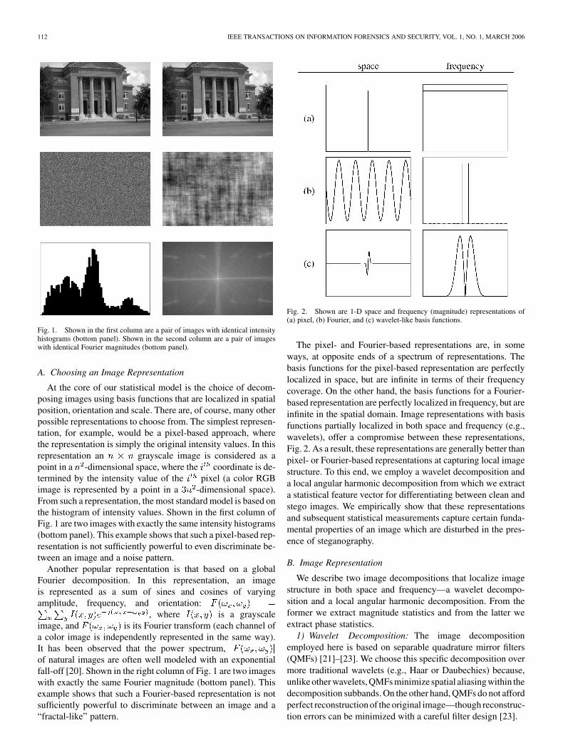
Fig. 1. Shown in the first column are a pair of images with identical intensityhistograms (bottom panel). Shown in the second column are a pair of imageswith identical Fourier magnitudes (bottom panel).

A. Choosing an Image Representation

At the core of our statistical model is the choice of decom-posing images using basis functions that are localized in spatialposition, orientation and scale. There are, of course, many otherpossible representations to choose from. The simplest represen-tation, for example, would be a pixel-based approach, wherethe representation is simply the original intensity values. In thisrepresentation an grayscale image is considered as apoint in a -dimensional space, where the coordinate is de-termined by the intensity value of the pixel (a color RGBimage is represented by a point in a -dimensional space).From such a representation, the most standard model is based onthe histogram of intensity values. Shown in the first column ofFig. 1 are two images with exactly the same intensity histograms(bottom panel). This example shows that such a pixel-based rep-resentation is not sufficiently powerful to even discriminate be-tween an image and a noise pattern.

Another popular representation is that based on a globalFourier decomposition. In this representation, an imageis represented as a sum of sines and cosines of varyingamplitude, frequency, and orientation:

, where is a grayscaleimage, and is its Fourier transform (each channel ofa color image is independently represented in the same way).It has been observed that the power spectrum,of natural images are often well modeled with an exponentialfall-off [20]. Shown in the right column of Fig. 1 are two imageswith exactly the same Fourier magnitude (bottom panel). Thisexample shows that such a Fourier-based representation is notsufficiently powerful to discriminate between an image and a“fractal-like” pattern.

Fig. 2. Shown are 1-D space and frequency (magnitude) representations of(a) pixel, (b) Fourier, and (c) wavelet-like basis functions.

The pixel- and Fourier-based representations are, in someways, at opposite ends of a spectrum of representations. Thebasis functions for the pixel-based representation are perfectlylocalized in space, but are infinite in terms of their frequencycoverage. On the other hand, the basis functions for a Fourier-based representation are perfectly localized in frequency, but areinfinite in the spatial domain. Image representations with basisfunctions partially localized in both space and frequency (e.g.,wavelets), offer a compromise between these representations,Fig. 2. As a result, these representations are generally better thanpixel- or Fourier-based representations at capturing local imagestructure. To this end, we employ a wavelet decomposition anda local angular harmonic decomposition from which we extracta statistical feature vector for differentiating between clean andstego images. We empirically show that these representationsand subsequent statistical measurements capture certain funda-mental properties of an image which are disturbed in the pres-ence of steganography.

B. Image Representation

We describe two image decompositions that localize imagestructure in both space and frequency—a wavelet decompo-sition and a local angular harmonic decomposition. From theformer we extract magnitude statistics and from the latter weextract phase statistics.

1) Wavelet Decomposition: The image decompositionemployed here is based on separable quadrature mirror filters(QMFs) [21]–[23]. We choose this specific decomposition overmore traditional wavelets (e.g., Haar or Daubechies) because,unlike other wavelets, QMFs minimize spatial aliasing within thedecomposition subbands. On the other hand, QMFs do not affordperfect reconstruction of the original image—though reconstruc-tion errors can be minimized with a careful filter design [23].

LYU AND FARID: STEGANALYSIS USING HIGHER-ORDER IMAGE STATISTICS 113

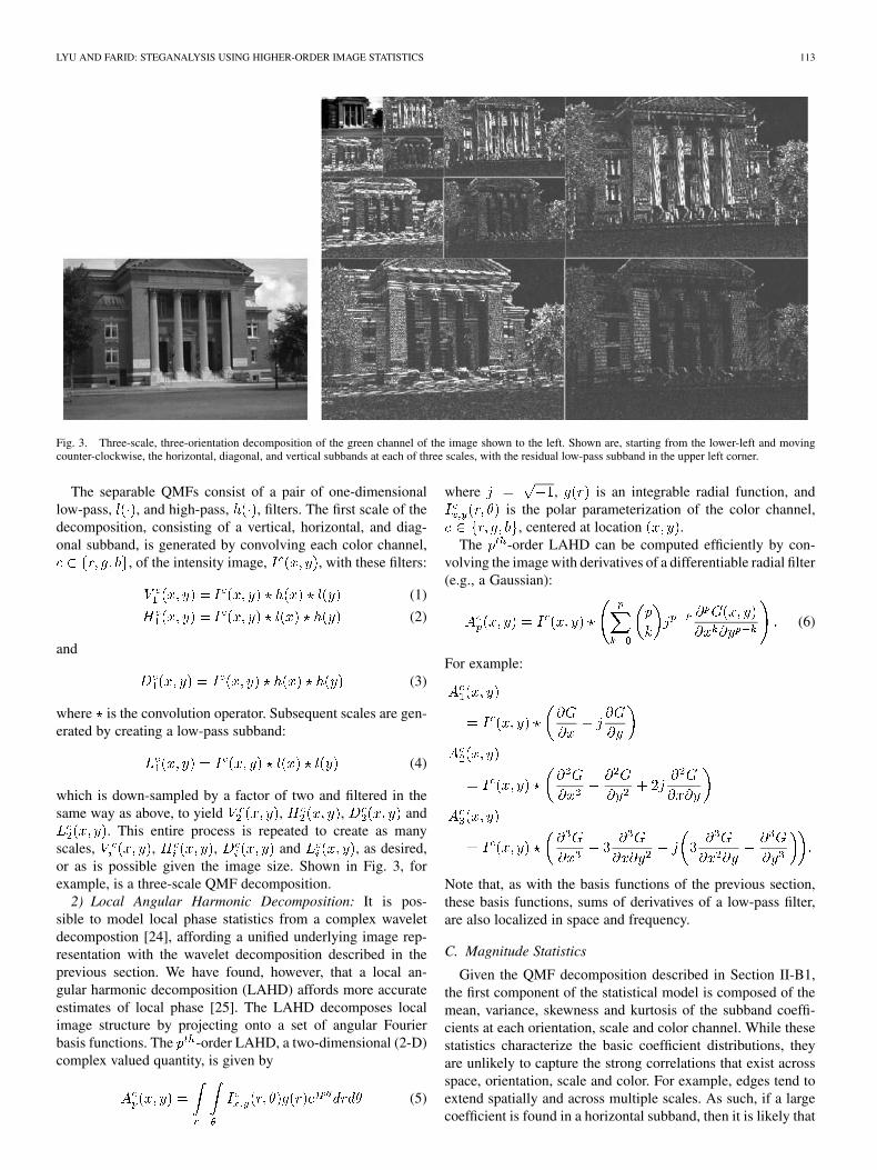
Fig. 3. Three-scale, three-orientation decomposition of the green channel of the image shown to the left. Shown are, starting from the lower-left and movingcounter-clockwise, the horizontal, diagonal, and vertical subbands at each of three scales, with the residual low-pass subband in the upper left corner.

The separable QMFs consist of a pair of one-dimensionallow-pass, , and high-pass, , filters. The first scale of thedecomposition, consisting of a vertical, horizontal, and diag-onal subband, is generated by convolving each color channel,

, of the intensity image, , with these filters:

(1)

(2)

and

(3)

where is the convolution operator. Subsequent scales are gen-erated by creating a low-pass subband:

(4)

which is down-sampled by a factor of two and filtered in thesame way as above, to yield , , and

. This entire process is repeated to create as manyscales, , , and , as desired,or as is possible given the image size. Shown in Fig. 3, forexample, is a three-scale QMF decomposition.

2) Local Angular Harmonic Decomposition: It is pos-sible to model local phase statistics from a complex waveletdecompostion [24], affording a unified underlying image rep-resentation with the wavelet decomposition described in theprevious section. We have found, however, that a local an-gular harmonic decomposition (LAHD) affords more accurateestimates of local phase [25]. The LAHD decomposes localimage structure by projecting onto a set of angular Fourierbasis functions. The -order LAHD, a two-dimensional (2-D)complex valued quantity, is given by

(5)

where , is an integrable radial function, andis the polar parameterization of the color channel,

, centered at location .The -order LAHD can be computed efficiently by con-

volving the image with derivatives of a differentiable radial filter(e.g., a Gaussian):

(6)

For example:

Note that, as with the basis functions of the previous section,these basis functions, sums of derivatives of a low-pass filter,are also localized in space and frequency.

C. Magnitude Statistics

Given the QMF decomposition described in Section II-B1,the first component of the statistical model is composed of themean, variance, skewness and kurtosis of the subband coeffi-cients at each orientation, scale and color channel. While thesestatistics characterize the basic coefficient distributions, theyare unlikely to capture the strong correlations that exist acrossspace, orientation, scale and color. For example, edges tend toextend spatially and across multiple scales. As such, if a largecoefficient is found in a horizontal subband, then it is likely that


its left and right spatial neighbors in the same subband will alsohave a large value. Similarly, a large coefficient at scale mightindicate a large value for its “parent” at scale .

In order to capture some of these higher-order statistical cor-relations, we collect a second set of statistics that are based onthe errors in a linear predictor of coefficient magnitude [26]. Forthe purpose of illustration, consider first a vertical band of thegreen channel at scale , . A linear predictor for themagnitude of these coefficients in a subset1 of all possible spa-tial, orientation, scale, and color neighbors is given by

(7)

where denotes absolute value and are the weights. Thislinear relationship can be expressed more compactly in matrixform as

(8)

where contains the coefficient magnitudes of strungout into a column vector, and the columns of the matrix con-tain the neighboring coefficient magnitudes as specified in (7),and . Only magnitudes greater than 1 are con-sidered, with the intensity values in the range [0,255]. Low mag-nitude coefficients are ignored when constructing the linear pre-dictor because we expect them to be less predictable from theirneighbors, and therefore less informative in capturing statisticalregularities. The weights are determined by minimizing thefollowing quadratic error function:

(9)

This error function is minimized by differentiating with respectto :

(10)

setting the result equal to zero, and solving for to yield theleast-squares estimate:

(11)

Given the large number of constraints (one per pixel) in onlynine unknowns, it is generally safe to assume that the 9 9matrix will be invertible.

Given the linear predictor, the log error between the actualcoefficient and the predicted coefficient magnitudes is

(12)

1The particular choice of neighbors was motivated by the observations of [26]and modified to include noncasual neighbors.

where the is computed point-wise on each vector compo-nent. It is from this error that additional statistics are collected,namely the mean, variance, skewness and kurtosis. This processis repeated for scales , and for the subbandsand , where the linear predictors for these subbands are ofthe form

(13)

and

(14)

A similar process is repeated for the horizontal and diagonalsubbands. As an example, the predictor for the green channeltakes the form

(15)

(16)

For the horizontal and diagonal subbands, the predictor for thered and blue channels are determined in a similar way as wasdone for the vertical subbands (13), (14). For each oriented,scale and color subband, a similar error metric, (12), and errorstatistics are computed.

For a decomposition with scales , the totalnumber of basic coefficient statistics is

, and the total number of error statisticsis also , yielding a total of statistics. Thesestatistics form the first half of the feature vector to be used todiscriminate between clean and stego images.


D. Phase Statistics

Given the local angular harmonic decomposition (LAHD) ofSection II-B2, a measure of relative phase, as described in [25],is computed as follows:

(17)

where is the angle between two complex numbers, and. From the relative phase, the following rotation

invariant signature, as described in [25], is computed:

(18)where denotes magnitude and .

From the 1st- through -order LAHDs, signa-tures are collected from within and across color channels (thereare combinations of LAHD orders, six orderedcombinations of color channels, and two statistics per combina-tion, yielding ). The phase statistics are collectedfrom the 2-D distribution of these signatures in the complexplane. Specifically, assuming zero-mean data, we consider thecovariance matrix:

(19)

where:

(20)

(21)

(22)

(23)

where is the total number of signatures, and andcorrespond to the real and imaginary components of a complexquantity. The structure of this covariance matrix is captured bythe measures:

(24)

and,

(25)

Considering this distribution as a scaled and rotated Gaussiandistribution, the first measure corresponds to the relative scalesalong the minor and major axes, and the second of these mea-sures to the orientation of the distribution.

In order to capture these phase statistics at various scales,this entire process is repeated for several levels of a Gaussianpyramid decomposition of the image [27]. These statistics formthe second half of the feature vector to be used to discriminatebetween clean and stego images.

E. Summary

Here we summarize the construction of the statistical featurevector from a color (RGB) image.

1) Build a -level, 3-orientation QMF pyramid for eachcolor channel (1)–(4).

2) For scales and for orientations , and, across all three color channels, , compute

the mean, variance, skewness, and kurtosis of the subbandcoefficients. This yields statistics.

3) For scales , and for orientations , and, across all three color channels, , build a

linear predictor of coefficient magnitude, (11). From theerror in the predictor, (12), compute the mean, variance,skewness, and kurtosis. This yields statistics.

4) Build a -level Gaussian pyramid for each color channel.For each level of the pyramid, compute the 1st- through

-order LAHD, (6). Compute the relative phases, (17).Compute the rotation invariant signature, (18), across allcolor channels and LAHD orders, from which the covari-ance matrix, (19), and subsequent phase statistics are ex-tracted, (24) and (25). This yields statistics.

III. CLASSIFICATION

From the measured statistics of a training set of clean andstego images, the goal is to determine whether a test imagecontains a hidden message. To this end, we employ supportvector machines (SVM) [28]–[30]. In the next section, weconsider the effectiveness of linear, nonlinear and one-classSVMs—see [13], [19] for the full details on the construction ofthese classifiers.

IV. RESULTS

We have collected 40 000 natural images.2 These colorimages span a range of indoor and outdoor scenes, are JPEGcompressed with an average quality of 90%, and typically are600 400 pixels in size (on average, 85.7 kilobytes). To contendwith slight variations in image size, only the central 256 256region of each image was considered in the analysis. Statistics, asdescribed in Section II, were collected from each image, yieldinga 432-D feature vector of magnitude and phase statistics. Forthe magnitude statistics, a four-level, three-orientation QMFpyramid was constructed using 9-tap filters, from which 108marginaland108error statisticswerecollected.For thephasesta-tistics a three-level Gaussian pyramid was constructed (using the5-tap binomial filter [1 4 6 4 1]/16), from which the 1st- through4th-order LAHDs are computed, to yield 216 phase statistics.3

Next, 40 000 stego images were generated by embeddingmessages of various sizes into the full-resolution cover images.The messages consisted of central regions of randomly chosenimages from the same image database with sizes 6.0, 4.7, 1.2,0.3 kilobytes (K), corresponding to 100%, 78%, 20% and 5%of total cover capacity. The total cover capacity is defined to bethe maximum size of a message that can be embedded by theembedding algorithm. Since this quantity will vary dependingon the cover image, we compute the average capacity across1000 cover images. The steganography capacity is then the ratiobetween the size of the embedded message and the total cover

2All natural images were downloaded from www.freefoto.com—all imageswere photographed with a range of different films, cameras, and lenses, anddigitally scanned.

3Since the N -order LAHD requires an N -order discrete derivative, thecomputation of higher-order LAHDs requires similarly higher-order derivatives.While computing higher-order discrete derivatives can be challenging, we findthat we are able to compute stable LAHDs up to 4th-order.


capacity. Messages were embedded using Jsteg [31], Outguess[32], Steghide [33], Jphide [34], and F5 [35]. Each stego imagewas generated with the same quality factor as the original coverimage so as to minimize double JPEG compression artifacts.The same statistical feature vector as described above wascomputed from the central 256 256 region of each stegoimage. In all of the results presented below, 32 000 of the cleanand stego images were used to train a SVM, and the remaining8000 images were used in testing—throughout, results fromthe testing stage are presented.

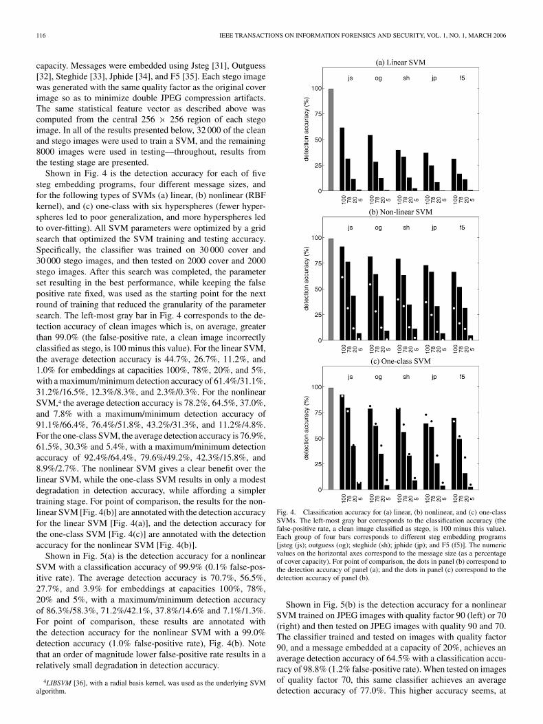
Shown in Fig. 4 is the detection accuracy for each of fivesteg embedding programs, four different message sizes, andfor the following types of SVMs (a) linear, (b) nonlinear (RBFkernel), and (c) one-class with six hyperspheres (fewer hyper-spheres led to poor generalization, and more hyperspheres ledto over-fitting). All SVM parameters were optimized by a gridsearch that optimized the SVM training and testing accuracy.Specifically, the classifier was trained on 30 000 cover and30 000 stego images, and then tested on 2000 cover and 2000stego images. After this search was completed, the parameterset resulting in the best performance, while keeping the falsepositive rate fixed, was used as the starting point for the nextround of training that reduced the granularity of the parametersearch. The left-most gray bar in Fig. 4 corresponds to the de-tection accuracy of clean images which is, on average, greaterthan 99.0% (the false-positive rate, a clean image incorrectlyclassified as stego, is 100 minus this value). For the linear SVM,the average detection accuracy is 44.7%, 26.7%, 11.2%, and1.0% for embeddings at capacities 100%, 78%, 20%, and 5%,with a maximum/minimum detection accuracy of 61.4%/31.1%,31.2%/16.5%, 12.3%/8.3%, and 2.3%/0.3%. For the nonlinearSVM,4 the average detection accuracy is 78.2%, 64.5%, 37.0%,and 7.8% with a maximum/minimum detection accuracy of91.1%/66.4%, 76.4%/51.8%, 43.2%/31.3%, and 11.2%/4.8%.For the one-class SVM, the average detection accuracy is 76.9%,61.5%, 30.3% and 5.4%, with a maximum/minimum detectionaccuracy of 92.4%/64.4%, 79.6%/49.2%, 42.3%/15.8%, and8.9%/2.7%. The nonlinear SVM gives a clear benefit over thelinear SVM, while the one-class SVM results in only a modestdegradation in detection accuracy, while affording a simplertraining stage. For point of comparison, the results for the non-linear SVM [Fig. 4(b)] are annotated with the detection accuracyfor the linear SVM [Fig. 4(a)], and the detection accuracy forthe one-class SVM [Fig. 4(c)] are annotated with the detectionaccuracy for the nonlinear SVM [Fig. 4(b)].

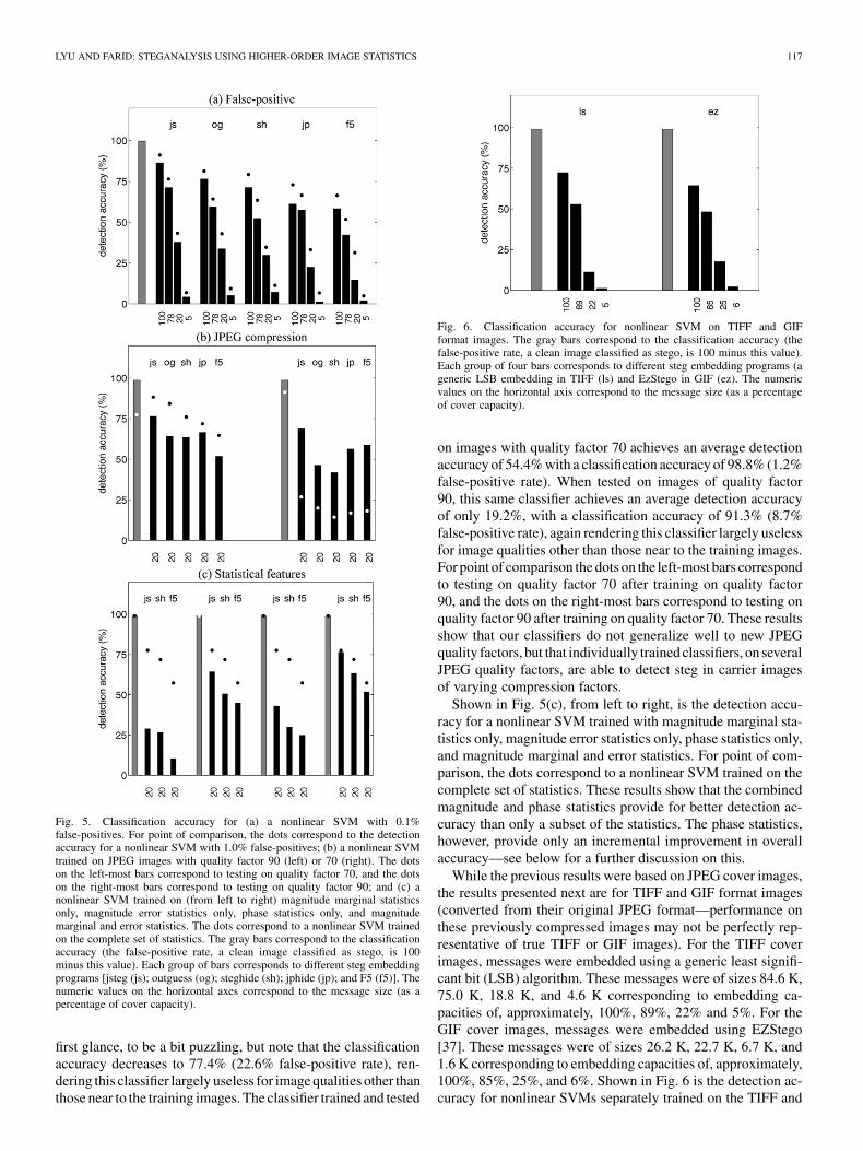
Shown in Fig. 5(a) is the detection accuracy for a nonlinearSVM with a classification accuracy of 99.9% (0.1% false-pos-itive rate). The average detection accuracy is 70.7%, 56.5%,27.7%, and 3.9% for embeddings at capacities 100%, 78%,20% and 5%, with a maximum/minimum detection accuracyof 86.3%/58.3%, 71.2%/42.1%, 37.8%/14.6% and 7.1%/1.3%.For point of comparison, these results are annotated withthe detection accuracy for the nonlinear SVM with a 99.0%detection accuracy (1.0% false-positive rate), Fig. 4(b). Notethat an order of magnitude lower false-positive rate results in arelatively small degradation in detection accuracy.

4LIBSVM [36], with a radial basis kernel, was used as the underlying SVMalgorithm.

Fig. 4. Classification accuracy for (a) linear, (b) nonlinear, and (c) one-classSVMs. The left-most gray bar corresponds to the classification accuracy (thefalse-positive rate, a clean image classified as stego, is 100 minus this value).Each group of four bars corresponds to different steg embedding programs[jsteg (js); outguess (og); steghide (sh); jphide (jp); and F5 (f5)]. The numericvalues on the horizontal axes correspond to the message size (as a percentageof cover capacity). For point of comparison, the dots in panel (b) correspond tothe detection accuracy of panel (a); and the dots in panel (c) correspond to thedetection accuracy of panel (b).

Shown in Fig. 5(b) is the detection accuracy for a nonlinearSVM trained on JPEG images with quality factor 90 (left) or 70(right) and then tested on JPEG images with quality 90 and 70.The classifier trained and tested on images with quality factor90, and a message embedded at a capacity of 20%, achieves anaverage detection accuracy of 64.5% with a classification accu-racy of 98.8% (1.2% false-positive rate). When tested on imagesof quality factor 70, this same classifier achieves an averagedetection accuracy of 77.0%. This higher accuracy seems, at


Fig. 5. Classification accuracy for (a) a nonlinear SVM with 0.1%false-positives. For point of comparison, the dots correspond to the detectionaccuracy for a nonlinear SVM with 1.0% false-positives; (b) a nonlinear SVMtrained on JPEG images with quality factor 90 (left) or 70 (right). The dotson the left-most bars correspond to testing on quality factor 70, and the dotson the right-most bars correspond to testing on quality factor 90; and (c) anonlinear SVM trained on (from left to right) magnitude marginal statisticsonly, magnitude error statistics only, phase statistics only, and magnitudemarginal and error statistics. The dots correspond to a nonlinear SVM trainedon the complete set of statistics. The gray bars correspond to the classificationaccuracy (the false-positive rate, a clean image classified as stego, is 100minus this value). Each group of bars corresponds to different steg embeddingprograms [jsteg (js); outguess (og); steghide (sh); jphide (jp); and F5 (f5)]. Thenumeric values on the horizontal axes correspond to the message size (as apercentage of cover capacity).

first glance, to be a bit puzzling, but note that the classificationaccuracy decreases to 77.4% (22.6% false-positive rate), ren-dering this classifier largely useless for image qualities other thanthose near to the training images. The classifier trained and tested

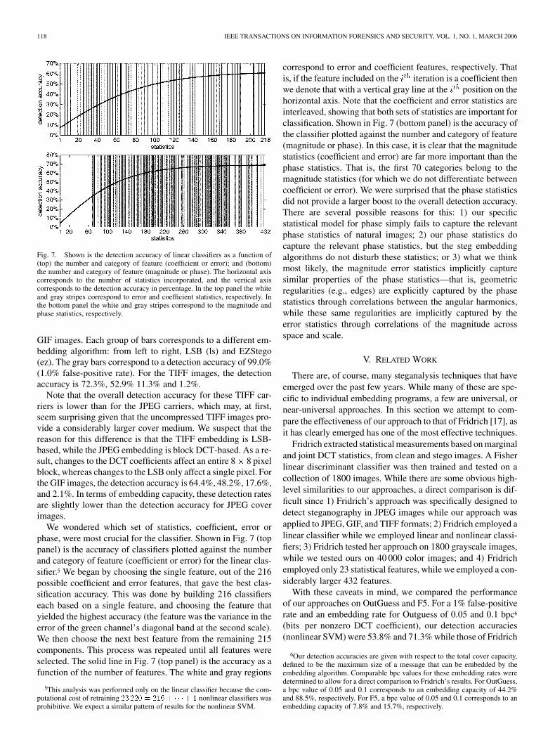
Fig. 6. Classification accuracy for nonlinear SVM on TIFF and GIFformat images. The gray bars correspond to the classification accuracy (thefalse-positive rate, a clean image classified as stego, is 100 minus this value).Each group of four bars corresponds to different steg embedding programs (ageneric LSB embedding in TIFF (ls) and EzStego in GIF (ez). The numericvalues on the horizontal axis correspond to the message size (as a percentageof cover capacity).

on images with quality factor 70 achieves an average detectionaccuracy of 54.4% with a classification accuracy of 98.8% (1.2%false-positive rate). When tested on images of quality factor90, this same classifier achieves an average detection accuracyof only 19.2%, with a classification accuracy of 91.3% (8.7%false-positive rate), again rendering this classifier largely uselessfor image qualities other than those near to the training images.For point of comparison the dots on the left-most bars correspondto testing on quality factor 70 after training on quality factor90, and the dots on the right-most bars correspond to testing onquality factor 90 after training on quality factor 70. These resultsshow that our classifiers do not generalize well to new JPEGquality factors, but that individually trained classifiers, on severalJPEG quality factors, are able to detect steg in carrier imagesof varying compression factors.

Shown in Fig. 5(c), from left to right, is the detection accu-racy for a nonlinear SVM trained with magnitude marginal sta-tistics only, magnitude error statistics only, phase statistics only,and magnitude marginal and error statistics. For point of com-parison, the dots correspond to a nonlinear SVM trained on thecomplete set of statistics. These results show that the combinedmagnitude and phase statistics provide for better detection ac-curacy than only a subset of the statistics. The phase statistics,however, provide only an incremental improvement in overallaccuracy—see below for a further discussion on this.

While the previous results were based on JPEG cover images,the results presented next are for TIFF and GIF format images(converted from their original JPEG format—performance onthese previously compressed images may not be perfectly rep-resentative of true TIFF or GIF images). For the TIFF coverimages, messages were embedded using a generic least signifi-cant bit (LSB) algorithm. These messages were of sizes 84.6 K,75.0 K, 18.8 K, and 4.6 K corresponding to embedding ca-pacities of, approximately, 100%, 89%, 22% and 5%. For theGIF cover images, messages were embedded using EZStego[37]. These messages were of sizes 26.2 K, 22.7 K, 6.7 K, and1.6 K corresponding to embedding capacities of, approximately,100%, 85%, 25%, and 6%. Shown in Fig. 6 is the detection ac-curacy for nonlinear SVMs separately trained on the TIFF and


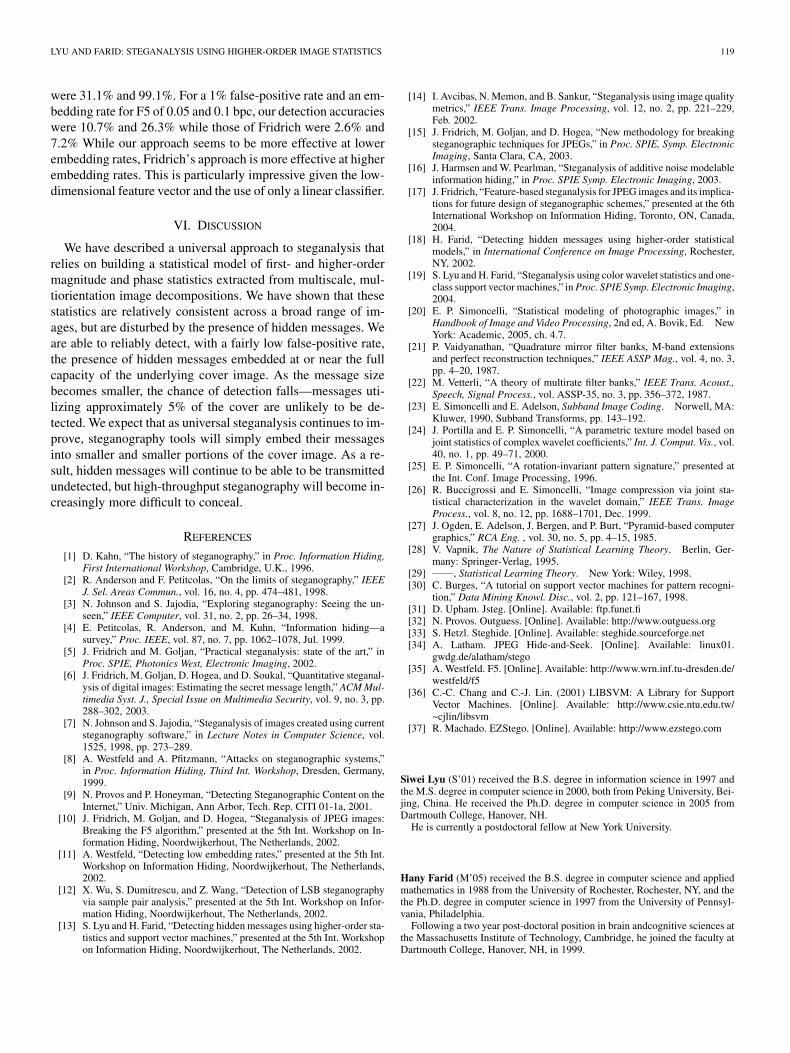
Fig. 7. Shown is the detection accuracy of linear classifiers as a function of(top) the number and category of feature (coefficient or error); and (bottom)the number and category of feature (magnitude or phase). The horizontal axiscorresponds to the number of statistics incorporated, and the vertical axiscorresponds to the detection accuracy in percentage. In the top panel the whiteand gray stripes correspond to error and coefficient statistics, respectively. Inthe bottom panel the white and gray stripes correspond to the magnitude andphase statistics, respectively.

GIF images. Each group of bars corresponds to a different em-bedding algorithm: from left to right, LSB (ls) and EZStego(ez). The gray bars correspond to a detection accuracy of 99.0%(1.0% false-positive rate). For the TIFF images, the detectionaccuracy is 72.3%, 52.9% 11.3% and 1.2%.

Note that the overall detection accuracy for these TIFF car-riers is lower than for the JPEG carriers, which may, at first,seem surprising given that the uncompressed TIFF images pro-vide a considerably larger cover medium. We suspect that thereason for this difference is that the TIFF embedding is LSB-based, while the JPEG embedding is block DCT-based. As a re-sult, changes to the DCT coefficients affect an entire 8 8 pixelblock, whereas changes to the LSB only affect a single pixel. Forthe GIF images, the detection accuracy is 64.4%, 48.2%, 17.6%,and 2.1%. In terms of embedding capacity, these detection ratesare slightly lower than the detection accuracy for JPEG coverimages.

We wondered which set of statistics, coefficient, error orphase, were most crucial for the classifier. Shown in Fig. 7 (toppanel) is the accuracy of classifiers plotted against the numberand category of feature (coefficient or error) for the linear clas-sifier.5 We began by choosing the single feature, out of the 216possible coefficient and error features, that gave the best clas-sification accuracy. This was done by building 216 classifierseach based on a single feature, and choosing the feature thatyielded the highest accuracy (the feature was the variance in theerror of the green channel’s diagonal band at the second scale).We then choose the next best feature from the remaining 215components. This process was repeated until all features wereselected. The solid line in Fig. 7 (top panel) is the accuracy as afunction of the number of features. The white and gray regions

5This analysis was performed only on the linear classifier because the com-putational cost of retraining 23220 = 216 + � � �+ 1 nonlinear classifiers wasprohibitive. We expect a similar pattern of results for the nonlinear SVM.

correspond to error and coefficient features, respectively. Thatis, if the feature included on the iteration is a coefficient thenwe denote that with a vertical gray line at the position on thehorizontal axis. Note that the coefficient and error statistics areinterleaved, showing that both sets of statistics are important forclassification. Shown in Fig. 7 (bottom panel) is the accuracy ofthe classifier plotted against the number and category of feature(magnitude or phase). In this case, it is clear that the magnitudestatistics (coefficient and error) are far more important than thephase statistics. That is, the first 70 categories belong to themagnitude statistics (for which we do not differentiate betweencoefficient or error). We were surprised that the phase statisticsdid not provide a larger boost to the overall detection accuracy.There are several possible reasons for this: 1) our specificstatistical model for phase simply fails to capture the relevantphase statistics of natural images; 2) our phase statistics docapture the relevant phase statistics, but the steg embeddingalgorithms do not disturb these statistics; or 3) what we thinkmost likely, the magnitude error statistics implicitly capturesimilar properties of the phase statistics—that is, geometricregularities (e.g., edges) are explicitly captured by the phasestatistics through correlations between the angular harmonics,while these same regularities are implicitly captured by theerror statistics through correlations of the magnitude acrossspace and scale.

V. RELATED WORK

There are, of course, many steganalysis techniques that haveemerged over the past few years. While many of these are spe-cific to individual embedding programs, a few are universal, ornear-universal approaches. In this section we attempt to com-pare the effectiveness of our approach to that of Fridrich [17], asit has clearly emerged has one of the most effective techniques.

Fridrich extracted statistical measurements based on marginaland joint DCT statistics, from clean and stego images. A Fisherlinear discriminant classifier was then trained and tested on acollection of 1800 images. While there are some obvious high-level similarities to our approaches, a direct comparison is dif-ficult since 1) Fridrich’s approach was specifically designed todetect steganography in JPEG images while our approach wasapplied to JPEG, GIF, and TIFF formats; 2) Fridrich employed alinear classifier while we employed linear and nonlinear classi-fiers; 3) Fridrich tested her approach on 1800 grayscale images,while we tested ours on 40 000 color images; and 4) Fridrichemployed only 23 statistical features, while we employed a con-siderably larger 432 features.

With these caveats in mind, we compared the performanceof our approaches on OutGuess and F5. For a 1% false-positiverate and an embedding rate for Outguess of 0.05 and 0.1 bpc6

(bits per nonzero DCT coefficient), our detection accuracies(nonlinear SVM) were 53.8% and 71.3% while those of Fridrich

6Our detection accuracies are given with respect to the total cover capacity,defined to be the maximum size of a message that can be embedded by theembedding algorithm. Comparable bpc values for these embedding rates weredetermined to allow for a direct comparison to Fridrich’s results. For OutGuess,a bpc value of 0.05 and 0.1 corresponds to an embedding capacity of 44.2%and 88.5%, respectively. For F5, a bpc value of 0.05 and 0.1 corresponds to anembedding capacity of 7.8% and 15.7%, respectively.


were 31.1% and 99.1%. For a 1% false-positive rate and an em-bedding rate for F5 of 0.05 and 0.1 bpc, our detection accuracieswere 10.7% and 26.3% while those of Fridrich were 2.6% and7.2% While our approach seems to be more effective at lowerembedding rates, Fridrich’s approach is more effective at higherembedding rates. This is particularly impressive given the low-dimensional feature vector and the use of only a linear classifier.

VI. DISCUSSION

We have described a universal approach to steganalysis thatrelies on building a statistical model of first- and higher-ordermagnitude and phase statistics extracted from multiscale, mul-tiorientation image decompositions. We have shown that thesestatistics are relatively consistent across a broad range of im-ages, but are disturbed by the presence of hidden messages. Weare able to reliably detect, with a fairly low false-positive rate,the presence of hidden messages embedded at or near the fullcapacity of the underlying cover image. As the message sizebecomes smaller, the chance of detection falls—messages uti-lizing approximately 5% of the cover are unlikely to be de-tected. We expect that as universal steganalysis continues to im-prove, steganography tools will simply embed their messagesinto smaller and smaller portions of the cover image. As a re-sult, hidden messages will continue to be able to be transmittedundetected, but high-throughput steganography will become in-creasingly more difficult to conceal.

REFERENCES

[1] D. Kahn, “The history of steganography,” in Proc. Information Hiding,First International Workshop, Cambridge, U.K., 1996.

[2] R. Anderson and F. Petitcolas, “On the limits of steganography,” IEEEJ. Sel. Areas Commun., vol. 16, no. 4, pp. 474–481, 1998.

[3] N. Johnson and S. Jajodia, “Exploring steganography: Seeing the un-seen,” IEEE Computer, vol. 31, no. 2, pp. 26–34, 1998.

[4] E. Petitcolas, R. Anderson, and M. Kuhn, “Information hiding—asurvey,” Proc. IEEE, vol. 87, no. 7, pp. 1062–1078, Jul. 1999.

[5] J. Fridrich and M. Goljan, “Practical steganalysis: state of the art,” inProc. SPIE, Photonics West, Electronic Imaging, 2002.

[6] J. Fridrich, M. Goljan, D. Hogea, and D. Soukal, “Quantitative steganal-ysis of digital images: Estimating the secret message length,” ACM Mul-timedia Syst. J., Special Issue on Multimedia Security, vol. 9, no. 3, pp.288–302, 2003.

[7] N. Johnson and S. Jajodia, “Steganalysis of images created using currentsteganography software,” in Lecture Notes in Computer Science, vol.1525, 1998, pp. 273–289.

[8] A. Westfeld and A. Pfitzmann, “Attacks on steganographic systems,”in Proc. Information Hiding, Third Int. Workshop, Dresden, Germany,1999.

[9] N. Provos and P. Honeyman, “Detecting Steganographic Content on theInternet,” Univ. Michigan, Ann Arbor, Tech. Rep. CITI 01-1a, 2001.

[10] J. Fridrich, M. Goljan, and D. Hogea, “Steganalysis of JPEG images:Breaking the F5 algorithm,” presented at the 5th Int. Workshop on In-formation Hiding, Noordwijkerhout, The Netherlands, 2002.

[11] A. Westfeld, “Detecting low embedding rates,” presented at the 5th Int.Workshop on Information Hiding, Noordwijkerhout, The Netherlands,2002.

[12] X. Wu, S. Dumitrescu, and Z. Wang, “Detection of LSB steganographyvia sample pair analysis,” presented at the 5th Int. Workshop on Infor-mation Hiding, Noordwijkerhout, The Netherlands, 2002.

[13] S. Lyu and H. Farid, “Detecting hidden messages using higher-order sta-tistics and support vector machines,” presented at the 5th Int. Workshopon Information Hiding, Noordwijkerhout, The Netherlands, 2002.

[14] I. Avcibas, N. Memon, and B. Sankur, “Steganalysis using image qualitymetrics,” IEEE Trans. Image Processing, vol. 12, no. 2, pp. 221–229,Feb. 2002.

[15] J. Fridrich, M. Goljan, and D. Hogea, “New methodology for breakingsteganographic techniques for JPEGs,” in Proc. SPIE, Symp. ElectronicImaging, Santa Clara, CA, 2003.

[16] J. Harmsen and W. Pearlman, “Steganalysis of additive noise modelableinformation hiding,” in Proc. SPIE Symp. Electronic Imaging, 2003.

[17] J. Fridrich, “Feature-based steganalysis for JPEG images and its implica-tions for future design of steganographic schemes,” presented at the 6thInternational Workshop on Information Hiding, Toronto, ON, Canada,2004.

[18] H. Farid, “Detecting hidden messages using higher-order statisticalmodels,” in International Conference on Image Processing, Rochester,NY, 2002.

[19] S. Lyu and H. Farid, “Steganalysis using color wavelet statistics and one-class support vector machines,” in Proc. SPIE Symp. Electronic Imaging,2004.

[20] E. P. Simoncelli, “Statistical modeling of photographic images,” inHandbook of Image and Video Processing, 2nd ed, A. Bovik, Ed. NewYork: Academic, 2005, ch. 4.7.

[21] P. Vaidyanathan, “Quadrature mirror filter banks, M-band extensionsand perfect reconstruction techniques,” IEEE ASSP Mag., vol. 4, no. 3,pp. 4–20, 1987.

[22] M. Vetterli, “A theory of multirate filter banks,” IEEE Trans. Acoust.,Speech, Signal Process., vol. ASSP-35, no. 3, pp. 356–372, 1987.

[23] E. Simoncelli and E. Adelson, Subband Image Coding. Norwell, MA:Kluwer, 1990, Subband Transforms, pp. 143–192.

[24] J. Portilla and E. P. Simoncelli, “A parametric texture model based onjoint statistics of complex wavelet coefficients,” Int. J. Comput. Vis., vol.40, no. 1, pp. 49–71, 2000.

[25] E. P. Simoncelli, “A rotation-invariant pattern signature,” presented atthe Int. Conf. Image Processing, 1996.

[26] R. Buccigrossi and E. Simoncelli, “Image compression via joint sta-tistical characterization in the wavelet domain,” IEEE Trans. ImageProcess., vol. 8, no. 12, pp. 1688–1701, Dec. 1999.

[27] J. Ogden, E. Adelson, J. Bergen, and P. Burt, “Pyramid-based computergraphics,” RCA Eng. , vol. 30, no. 5, pp. 4–15, 1985.

[28] V. Vapnik, The Nature of Statistical Learning Theory. Berlin, Ger-many: Springer-Verlag, 1995.

[29] , Statistical Learning Theory. New York: Wiley, 1998.[30] C. Burges, “A tutorial on support vector machines for pattern recogni-

tion,” Data Mining Knowl. Disc., vol. 2, pp. 121–167, 1998.[31] D. Upham. Jsteg. [Online]. Available: ftp.funet.fi[32] N. Provos. Outguess. [Online]. Available: http://www.outguess.org[33] S. Hetzl. Steghide. [Online]. Available: steghide.sourceforge.net[34] A. Latham. JPEG Hide-and-Seek. [Online]. Available: linux01.

gwdg.de/alatham/stego[35] A. Westfeld. F5. [Online]. Available: http://www.wrn.inf.tu-dresden.de/

westfeld/f5[36] C.-C. Chang and C.-J. Lin. (2001) LIBSVM: A Library for Support

Vector Machines. [Online]. Available: http://www.csie.ntu.edu.tw/~cjlin/libsvm

[37] R. Machado. EZStego. [Online]. Available: http://www.ezstego.com

Siwei Lyu (S’01) received the B.S. degree in information science in 1997 andthe M.S. degree in computer science in 2000, both from Peking University, Bei-jing, China. He received the Ph.D. degree in computer science in 2005 fromDartmouth College, Hanover, NH.

He is currently a postdoctoral fellow at New York University.

Hany Farid (M’05) received the B.S. degree in computer science and appliedmathematics in 1988 from the University of Rochester, Rochester, NY, and thethe Ph.D. degree in computer science in 1997 from the University of Pennsyl-vania, Philadelphia.

Following a two year post-doctoral position in brain andcognitive sciences atthe Massachusetts Institute of Technology, Cambridge, he joined the faculty atDartmouth College, Hanover, NH, in 1999.

Steganalysis using higher-order image statistics

Documents