Statistics in Monte Carlo Analysis - FlowCAD

Statistics in Monte Carlo Analysis

PSpice Application Note │ V2

Statistics in Monte Carlo Analysis, V2 FlowCAD Confidential │

2

Table of Contents 1 Introduction .................................................................................................................... 3

2 Demo Project .................................................................................................................. 4

3 Bibliography ................................................................................................................. 15


3

1 Introduction The Monte Carlo analysis calculates the circuit response to changes in part values by randomly varying all of the model parameters for which a tolerance is specified. This provides statistical data on the impact of a device parameter’s variance. Monte Carlo analysis is frequently used to predict yields on production runs of a circuit. With Monte Carlo analysis, model parameters are given tolerances, and multiple analyses (DC, AC, or transient) are run using these tolerances.

You can display data derived from Monte Carlo waveform families as histograms (using Performance Analysis).

Fig. 1: Histogram of Max(I(Meter))

The MONTE CARLO SUMMARY depended on the collating function e.g. the greatest difference from the nominal run (YMAX) is reported in PSpice output file.

Fig. 2: MONTE CARLO SUMMARY in PSpice Output File

But how can we understand the statistical data?


4

2 Demo Project The following example shows how the performance of a pressure sensor circuit with a pressure-dependent resistor bridge is affected by manufacturing tolerances, using Monte Carlo analysis to explore these effects.

A zero volt voltage source is commonly used as a current meter in PSpice. A zero ohm resistor is not allowed.

In the above circuit, the model with the following definition .model Rmc RES R=1 DEV=2% LOT=8%

is assigned to resistors R1, R2, R3 and R_Pressure while R4, R5 and R6 are normal resistors without tolerance.

Note

• Both tolerances DEV and LOT are available for each model parameter. Device tolerances, denoted as DEV within the model statement, cause components that share the same model to vary independently of one another. Lot tolerances, denoted by LOT in the model statement, cause components that share a common model to vary together.

• If you want to apply only a DEV tolerance to a usual R, L or C device, you can edit the TOLERANCE attribute on the part.

• To add both LOT and DEV tolerance to R, L and C devices, you must use the breakout symbols Rbreak, Lbreak and Cbreak in place of the usual R, L and C parts.

R1

Rmc1k

R2

Rmc1k

R_Pressure

Rmc{1K*(1+P*PCoef f /Pnom)}

R3

Rmc1k

R5

1k

R61k

V11.35V

0

PARAMETERS:Pcoef f = -0.06Pnom = 1.0P = 1Meter

0Vdc

R4

1k


5

Simulation Settings and Simulation Results The simulation profile could be a DC Sweep analysis as follows:

In Monte Carlo/Worst Case option, set I(Meter) as the Output variable, use Gaussian as distribution. If you left Random number seed blank, the default value 17533 will be used for the random number generator.


6

Note

• It is possible to set different distribution for different components but this needs to be done at model level. The distributions defined in the .model statement override the setting in the simulation setting options for MC analysis. For example:

.model Rmc1 RES R=1 DEV/UNIFORM=2% LOT/UNIFORM=8%

.model Rmc2 RES R=1 DEV/GAUSSIAN=2% LOT/GAUSSIAN=8%

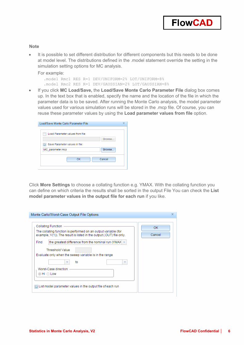
• If you click MC Load/Save, the Load/Save Monte Carlo Parameter File dialog box comes up. In the text box that is enabled, specify the name and the location of the file in which the parameter data is to be saved. After running the Monte Carlo analysis, the model parameter values used for various simulation runs will be stored in the .mcp file. Of course, you can reuse these parameter values by using the Load parameter values from file option.

Click More Settings to choose a collating function e.g. YMAX. With the collating function you can define on which criteria the results shall be sorted in the output File You can check the List model parameter values in the output file for each run if you like.


7

After the simulation the curves of I(Meter) could be as follows:

Note

With many runs (100 runs in our case), the waveform display can look more like a band than a set of individual waveforms. This can be useful for seeing the typical spread for a particular output variable. As the number of runs increases, the spread more closely approximates the actual worst-case limits for the circuit.

Click the Performance Analysis button, add trace Max(I(Meter)) to display histograms.


8

A MONTE CARLO SUMMARY is reported according to the output variable in simulation set up and the used collating function. The deviations are printed in order of size along with their run number.

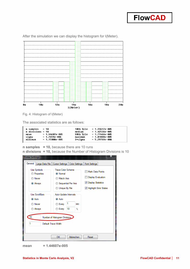
The Quantity of the bars in the bar chart (histogram) can be set under Tools > Options > Number of Histogram Divisions.

Fig. 3: MONTE CARLO SUMMARY with original Simulation Settings

Note

When you use the YMAX collating function, the output file also lists mean deviation and sigma values. These are based on the changes in the output variable from nominal at every sweep point in every Monte Carlo run.

MONTE CARLO SUMMARY In the above diagram, the first RUN is Pass 28, because the deviation from nominal is the biggest in all of the Monte Carlo runs.

The maximal deviation is 5.4934E-06 (2.25 sigma), because of 2.4445E-06*2.25≈5.500E-06.

Higher at P=3.6 means I(Meter) at the 28th run is bigger than at the nominal run while the sweep parameter P=3.6.

Note

There could be some rounding errors while calculating. The exact value is not very important here, the point is to understand the methodology within Monte Carlo analysis.

If you are interested which parameter values are used at pass 28, you can get the information in PSpice output file (the parameter values are also saved in MC_parameter.mcp).


9

Now go back to Simulation Settings window and set the sweep variable P=3.6 and run the simulation again.

The new simulation results could be as follows:


10

Just marking I(Meter) > Edit > Copy, then open the Texteditor and paste the data, save the file as e.g. my_data.txt.

In this file you will get I(Meter)

• at the nominal run is 1.3759909052169e-005 • at the 28th run is 1.92532643268351e-005

Note

In MC analysis, the first run is always the nominal run.

Therefore, the difference is: 1.92532643268351e-005 - 1.3759909052169e-005 ≈ 5.4934e-006

Please look at the MAX DEVIATION FROM NOMINAL at Pass 28 in MONTE CARLO SUMMARY section in PSpice output file (see Fig. 3), it is 5.4934E-06 and the same as our calculated value.

There is still 139.92% of Nominal because 1.92532643268351e-005/1.3759909052169e-005 ≈ 139.92%.

Histogram and Statistical Data Here we would like to reduce the number of runs to have less data for better calculation. But in fact, you may need much more runs to get more reasonable statistical data.

The sweep variable P remains with the value 3.6 and we just reduce the number of runs from 100 to 10.


11

After the simulation we can display the histogram for I(Meter).

Fig. 4: Histogram of I(Meter)

The associated statistics are as follows:

n samples = 10, because there are 10 runs n divisions = 10, because the Number of Histogram Divisions is 10

mean = 1.44607e-005


12

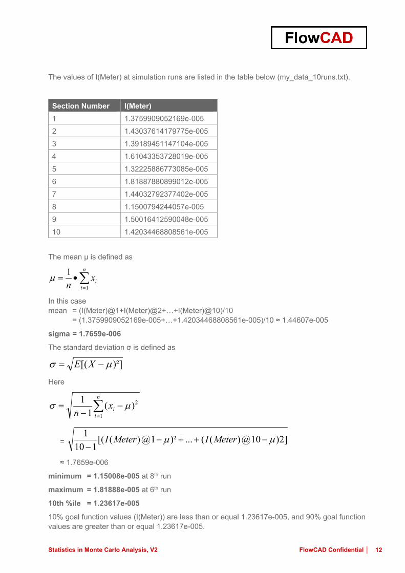
The values of I(Meter) at simulation runs are listed in the table below (my_data_10runs.txt).

Section Number I(Meter) 1 1.3759909052169e-005 2 1.43037614179775e-005 3 1.39189451147104e-005 4 1.61043353728019e-005 5 1.32225886773085e-005 6 1.81887880899012e-005 7 1.44032792377402e-005 8 1.1500794244057e-005 9 1.50016412590048e-005 10 1.42034468808561e-005

The mean µ is defined as

∑=

•=n

iix

n 1

1µ

In this case mean = (I(Meter)@1+I(Meter)@2+…+I(Meter)@10)/10 = (1.3759909052169e-005+…+1.42034468808561e-005)/10 ≈ 1.44607e-005

sigma = 1.7659e-006

The standard deviation σ is defined as

)²][( µσ −= XE

Here

∑=

−−

=n

iix

n 1

2)(1

1 µσ

= ]2)10@)((...)²1@)([(110

1 µµ −++−−

MeterIMeterI

≈ 1.7659e-006

minimum = 1.15008e-005 at 8th run

maximum = 1.81888e-005 at 6th run

10th %ile = 1.23617e-005

10% goal function values (I(Meter)) are less than or equal 1.23617e-005, and 90% goal function values are greater than or equal 1.23617e-005.


13

)(21

1

~

+•• += pnpnp xxx , if n●p integral,

pnxxp •=~

, if n●p not integral

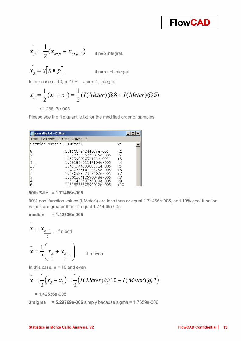
In our case n=10, p=10% → n●p=1, integral

)5@)(8@)((21)(

21

21

~MeterIMeterIxxxp +=+=

≈ 1.23617e-005

Please see the file quantile.txt for the modified order of samples.

90th %ile = 1.71466e-005

90% goal function values (I(Meter)) are less than or equal 1.71466e-005, and 10% goal function values are greater than or equal 1.71466e-005.

median = 1.42536e-005

21

~

+= nxx , if n odd

+=

+122

~

21

nn xxx , if n even

In this case, n = 10 and even

( ) ( )2@)(10@)(21

21

65

~MeterIMeterIxxx +=+=

= 1.42536e-005

3*sigma = 5.29769e-006 simply because sigma = 1.7659e-006


14

Difference of the Statistical Data Reported in Histogram and in Output File

The statistical data in histogram are for the samples measured using a function, e.g. Max(I(Meter)) in Fig. 1 or using a simulation output variable in Add Traces window, e.g. I(Meter) in Fig. 4. A histogram has nothing to do with the collating function.

The statistical data in output file are based on the output variable defined in Simulation Settings and the collating function. For example, the MONTE CARLO SUMMARY looks as follows:

In this case there are 9 samples, not 10 samples. The sample value is the maximal deviation from nominal, not the value of a measurement or an available output variable.

Mean Deviation = 778.7100E-09

Here:

∑=

=n

iix

ndeviationmean

1

1

≈ 778.71E-09


15

Please refer deviation.txt file which based on the data of MONTE CARLO SUMMARY. The values (x7 and x3) are negative, because they are lower than the nominal.

Sigma = 1.7486E-06

In our case

( )∑=

−=n

ii DeviationMeanx

nSigma

1

21

≈ 1.7486E-06

3 Bibliography [1] PSpice User Guide, Cadence

[2] PSpice Reference Guide, Cadence

[3] OrCAD Capture User Guide, Cadence

[4] http://de.wikipedia.org/wiki/Quantil

[5] http://de.wikipedia.org/wiki/Standardabweichung

http://de.wikipedia.org/wiki/Quantil

http://de.wikipedia.org/wiki/Standardabweichung

Statistics in Monte Carlo Analysis - FlowCAD

Documents