Statistically Rigorous Java Performance Evaluation Andy Georges Dries Buytaert Lieven Eeckhout Department of Electronics and Information Systems, Ghent University, Belgium {ageorges,dbuytaer,leeckhou}@elis.ugent.be Abstract Java performance is far from being trivial to benchmark because it is affected by various factors such as the Java application, its input, the virtual machine, the garbage collector, the heap size, etc. In addition, non-determinism at run-time causes the execution time of a Java program to differ from run to run. There are a number of sources of non-determinism such as Just-In-Time (JIT) compilation and optimization in the virtual machine (VM) driven by timer- based method sampling, thread scheduling, garbage collection, and various system effects. There exist a wide variety of Java performance evaluation methodologies used by researchers and benchmarkers. These methodologies differ from each other in a number of ways. Some report average performance over a number of runs of the same experiment; others report the best or second best performance ob- served; yet others report the worst. Some iterate the benchmark multiple times within a single VM invocation; others consider mul- tiple VM invocations and iterate a single benchmark execution; yet others consider multiple VM invocations and iterate the benchmark multiple times. This paper shows that prevalent methodologies can be mis- leading, and can even lead to incorrect conclusions. The reason is that the data analysis is not statistically rigorous. In this pa- per, we present a survey of existing Java performance evaluation methodologies and discuss the importance of statistically rigorous data analysis for dealing with non-determinism. We advocate ap- proaches to quantify startup as well as steady-state performance, and, in addition, we provide the JavaStats software to automatically obtain performance numbers in a rigorous manner. Although this paper focuses on Java performance evaluation, many of the issues addressed in this paper also apply to other programming languages and systems that build on a managed runtime system. Categories and Subject Descriptors D.2.8 [Software En- gineering]: Metrics—Performance measures; D.3.4 [Pro- gramming Languages]: Processors—Run-time environments Permission to make digital or hard copies of all or part of this work for personal or classroom use is granted without fee provided that copies are not made or distributed for profit or commercial advantage and that copies bear this notice and the full citation on the first page. To copy otherwise, to republish, to post on servers or to redistribute to lists, requires prior specific permission and/or a fee. OOPSLA’07, October 21–25, 2007, Montr´ eal, Qu´ ebec, Canada. Copyright c 2007 ACM 978-1-59593-786-5/07/0010. . . $5.00 General Terms Experimentation, Measurement, Perfor- mance Keywords Java, benchmarking, data analysis, methodol- ogy, statistics 1. Introduction Benchmarking is at the heart of experimental computer sci- ence research and development. Market analysts compare commercial products based on published performance num- bers. Developers benchmark products under development to assess their performance. And researchers use benchmark- ing to evaluate the impact on performance of their novel re- search ideas. As such, it is absolutely crucial to have a rig- orous benchmarking methodology. A non-rigorous method- ology may skew the overall picture, and may even lead to incorrect conclusions. And this may drive research and de- velopment in a non-productive direction, or may lead to a non-optimal product brought to market. Managed runtime systems are particularly challenging to benchmark because there are numerous factors affect- ing overall performance, which is of lesser concern when it comes to benchmarking compiled programming languages such as C. Benchmarkers are well aware of the difficulty in quantifying managed runtime system performance which is illustrated by a number of research papers published over the past few years showing the complex interactions between low-level events and overall performance [5, 11, 12, 17, 24]. More specifically, recent work on Java performance method- ologies [7, 10] stressed the importance of a well chosen and well motivated experimental design: it was pointed out that the results presented in a Java performance study are subject to the benchmarks, the inputs, the VM, the heap size, and the hardware platform that are chosen in the experimental setup. Not appropriately considering and motivating one of these key aspects, or not appropriately describing the context within which the results were obtained and how they should be interpreted may give a skewed view, and may even be misleading or at worst be incorrect. The orthogonal axis to experimental design in a perfor- mance evaluation methodology, is data analysis, or how to analyze and report the results. More specifically, a per- formance evaluation methodology needs to adequately deal

Welcome message from author
This document is posted to help you gain knowledge. Please leave a comment to let me know what you think about it! Share it to your friends and learn new things together.
Transcript
Statistically Rigorous Java Performance Evaluation
Andy Georges Dries Buytaert Lieven EeckhoutDepartment of Electronics and Information Systems, Ghent University, Belgium
{ageorges,dbuytaer,leeckhou}@elis.ugent.be
AbstractJava performance is far from being trivial to benchmark becauseit is affected by various factors such as the Java application, itsinput, the virtual machine, the garbage collector, the heap size, etc.In addition, non-determinism at run-time causes the execution timeof a Java program to differ from run to run. There are a number ofsources of non-determinism such as Just-In-Time (JIT) compilationand optimization in the virtual machine (VM) driven by timer-based method sampling, thread scheduling, garbage collection, andvarious system effects.
There exist a wide variety of Java performance evaluationmethodologies used by researchers and benchmarkers. Thesemethodologies differ from each other in a number of ways. Somereport average performance over a number of runs of the sameexperiment; others report the best or second best performance ob-served; yet others report the worst. Some iterate the benchmarkmultiple times within a single VM invocation; others consider mul-tiple VM invocations and iterate a single benchmark execution; yetothers consider multiple VM invocations and iterate the benchmarkmultiple times.
This paper shows that prevalent methodologies can be mis-leading, and can even lead to incorrect conclusions. The reasonis that the data analysis is not statistically rigorous. In this pa-per, we present a survey of existing Java performance evaluationmethodologies and discuss the importance of statistically rigorousdata analysis for dealing with non-determinism. We advocate ap-proaches to quantify startup as well as steady-state performance,and, in addition, we provide the JavaStats software to automaticallyobtain performance numbers in a rigorous manner. Although thispaper focuses on Java performance evaluation, many of the issuesaddressed in this paper also apply to other programming languagesand systems that build on a managed runtime system.
Categories and Subject Descriptors D.2.8 [Software En-gineering]: Metrics—Performance measures; D.3.4 [Pro-gramming Languages]: Processors—Run-time environments
Permission to make digital or hard copies of all or part of this work for personal orclassroom use is granted without fee provided that copies are not made or distributedfor profit or commercial advantage and that copies bear this notice and the full citationon the first page. To copy otherwise, to republish, to post on servers or to redistributeto lists, requires prior specific permission and/or a fee.OOPSLA’07, October 21–25, 2007, Montreal, Quebec, Canada.Copyright c© 2007 ACM 978-1-59593-786-5/07/0010. . . $5.00
General Terms Experimentation, Measurement, Perfor-mance
Keywords Java, benchmarking, data analysis, methodol-ogy, statistics
1. IntroductionBenchmarking is at the heart of experimental computer sci-ence research and development. Market analysts comparecommercial products based on published performance num-bers. Developers benchmark products under development toassess their performance. And researchers use benchmark-ing to evaluate the impact on performance of their novel re-search ideas. As such, it is absolutely crucial to have a rig-orous benchmarking methodology. A non-rigorous method-ology may skew the overall picture, and may even lead toincorrect conclusions. And this may drive research and de-velopment in a non-productive direction, or may lead to anon-optimal product brought to market.
Managed runtime systems are particularly challengingto benchmark because there are numerous factors affect-ing overall performance, which is of lesser concern when itcomes to benchmarking compiled programming languagessuch as C. Benchmarkers are well aware of the difficulty inquantifying managed runtime system performance which isillustrated by a number of research papers published over thepast few years showing the complex interactions betweenlow-level events and overall performance [5, 11, 12, 17, 24].More specifically, recent work on Java performance method-ologies [7, 10] stressed the importance of a well chosen andwell motivated experimental design: it was pointed out thatthe results presented in a Java performance study are subjectto the benchmarks, the inputs, the VM, the heap size, andthe hardware platform that are chosen in the experimentalsetup. Not appropriately considering and motivating one ofthese key aspects, or not appropriately describing the contextwithin which the results were obtained and how they shouldbe interpreted may give a skewed view, and may even bemisleading or at worst be incorrect.
The orthogonal axis to experimental design in a perfor-mance evaluation methodology, is data analysis, or howto analyze and report the results. More specifically, a per-formance evaluation methodology needs to adequately deal
with the non-determinism in the experimental setup. In aJava system, or managed runtime system in general, thereare a number of sources of non-determinism that affect over-all performance. One potential source of non-determinism isJust-In-Time (JIT) compilation. A virtual machine (VM) thatuses timer-based sampling to drive the VM compilation andoptimization subsystem may lead to non-determinism andexecution time variability: different executions of the sameprogram may result in different samples being taken and,by consequence, different methods being compiled and op-timized to different levels of optimization. Another sourceof non-determinism comes from thread scheduling in time-shared and multiprocessor systems. Running multithreadedworkloads, as is the case for most Java programs, requiresthread scheduling in the operating system and/or virtual ma-chine. Different executions of the same program may in-troduce different thread schedules, and may result in dif-ferent interactions between threads, affecting overall per-formance. The non-determinism introduced by JIT compi-lation and thread scheduling may affect the points in timewhere garbage collections occur. Garbage collection in itsturn may affect program locality, and thus memory systemperformance as well as overall system performance. Yet an-other source of non-determinism is various system effects,such as system interrupts — this is not specific to managedruntime systems though as it is a general concern when run-ning experiments on real hardware.
From an extensive literature survey, we found that thereare a plethora of prevalent approaches, both in experimen-tal design and data analysis for benchmarking Java perfor-mance. Prevalent data analysis approaches for dealing withnon-determinism are not statistically rigorous though. Somereport the average performance number across multiple runsof the same experiments; others report the best performancenumber, others report the second best performance numberand yet others report the worst. In this paper, we argue thatnot appropriately specifying the experimental design and notusing a statistically rigorous data analysis can be mislead-ing and can even lead to incorrect conclusions. This paperadvocates using statistics theory as a rigorous data analysisapproach for dealing with the non-determinism in managedruntime systems.
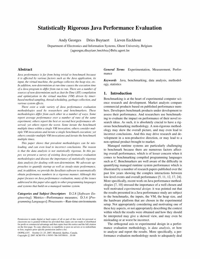
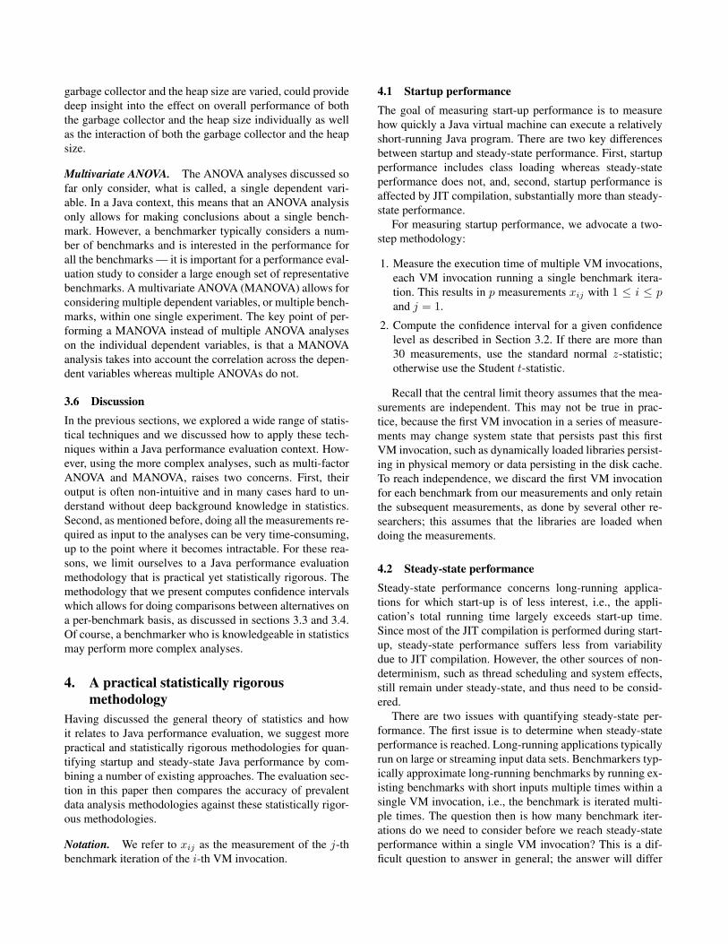
The pitfall in using a prevalent method is illustrated inFigure 1 which compares the execution time for runningJikes RVM with five garbage collectors (CopyMS, GenCopy,GenMS, MarkSweep and SemiSpace) for the SPECjvm98db benchmark with a 120MB heap size — the experi-mental setup will be detailed later. This graph comparesthe prevalent ‘best’ method which reports the best perfor-mance number (or smallest execution time) among 30 mea-surements against a statistically rigorous method which re-ports 95% confidence intervals; the ‘best’ method does notcontrol non-determinism, and corresponds to the SPEC re-porting rules [23]. Based on the best method, one would
mean w/ 95% confidence interval
9.0
9.5
10.0
10.5
11.0
11.5
12.0
12.5
CopyM
S
Gen
Copy
Gen
MS
Mar
kSw
eep
Sem
iSpace
exec
ution t
ime
(s)
best of 30
9.0
9.5
10.0
10.5
11.0
11.5
12.0
12.5
CopyM
S
Gen
Copy
Gen
MS
Mar
kSw
eep
Sem
iSpace
exec
ution t
ime
(s)
Figure 1. An example illustrating the pitfall of prevalentJava performance data analysis methods: the ‘best’ methodis shown on the left and the statistically rigorous method isshown on the right. This is for db and a 120MB heap size.
conclude that the performance for the CopyMS and Gen-Copy collectors is about the same. The statistically rigorousmethod though shows that GenCopy significantly outper-forms CopyMS. Similarly, based on the best method, onewould conclude that SemiSpace clearly outperforms Gen-Copy. The reality though is that the confidence intervals forboth garbage collectors overlap and, as a result, the per-formance difference seen between both garbage collectorsis likely due to the random performance variations in thesystem under measurement. In fact, we observe a large per-formance variation for SemiSpace, and at least one reallygood run along with a large number of less impressive runs.The ‘best’ method reports the really good run whereas a sta-tistically rigorous approach reliably reports that the averagescores for GenCopy and SemiSpace are very close to eachother.
This paper makes the following contributions:
• We demonstrate that there is a major pitfall associ-ated with today’s prevalent Java performance evaluationmethodologies, especially in terms of data analysis. Thepitfall is that they may yield misleading and even in-correct conclusions. The reason is that the data analysisemployed by these methodologies is not statistically rig-orous.
• We advocate adding statistical rigor to performance eval-uation studies of managed runtime systems, and in partic-ular Java systems. The motivation for statistically rigor-ous data analysis is that statistics, and in particular con-fidence intervals, enable one to determine whether dif-ferences observed in measurements are due to randomfluctuations in the measurements or due to actual differ-ences in the alternatives compared against each other. Wediscuss how to compute confidence intervals and discusstechniques to compare multiple alternatives.
• We survey existing performance evaluation methodolo-gies for start-up and steady-state performance, and ad-vocate the following methods. For start-up performance,we advise to: (i) take multiple measurements where each
measurement comprises one VM invocation and a sin-gle benchmark iteration, and (ii) compute confidence in-tervals across these measurements. For steady-state per-formance, we advise to: (i) take multiple measurementswhere each measurement comprises one VM invocationand multiple benchmark iterations, (ii) in each of thesemeasurements, collect performance numbers for differ-ent iterations once performance reaches steady-state, i.e.,after the start-up phase, and (iii) compute confidence in-tervals across these measurements (multiple benchmarkiterations across multiple VM invocations).
• We provide publicly available software, called JavaStats,to enable a benchmarker to easily collect the informationrequired to do a statistically rigorous Java performanceanalysis. In particular, JavaStats monitors the variabilityobserved in the measurements to determine the numberof measurements that need to be taken to reach a desiredconfidence interval for a given confidence level. Java-Stats readily works for both the SPECjvm98 and DaCapobenchmark suites, and is available athttp://www.elis.ugent.be/JavaStats.
This paper is organized as follows. We first present a sur-vey in Section 2 on Java performance evaluation method-ologies in use today. Subsequently, in Section 3, we discussgeneral statistics theory and how it applies to Java perfor-mance analysis. Section 4 then translates these theoreticalconcepts to practical methodologies for quantifying startupand steady-state performance. After detailing our experi-mental setup in Section 5, we then assess in Section 6 theprevalent evaluation methodologies compared to the statis-tically rigorous methodologies advocated in this paper. Weshow that in many practical situations, prevalent methodolo-gies can be misleading, or even yield incorrect conclusions.Finally, we summarize and conclude in Section 7.
2. Prevalent Java Performance EvaluationMethodologies
There is a wide range of Java performance evaluationmethodologies in use today. In order to illustrate this, wehave performed a survey among the Java performance pa-pers published in the last few years (from 2000 onwards) inpremier conferences such as Object-Oriented Programming,Systems, Languages and Applications (OOPSLA), Pro-gramming Language Design and Implementation (PLDI),Virtual Execution Environments (VEE), Memory Man-agement (ISMM) and Code Generation and Optimization(CGO). In total, we examined the methodology used in 50papers.
Surprisingly enough, about one third of the papers (16out of the 50 papers) does not specify the methodologyused in the paper. This not only makes it difficult for otherresearchers to reproduce the results presented in the paper, italso makes understanding and interpreting the results hard.
During our survey, we found that not specifying or onlypartially specifying the performance evaluation methodol-ogy is particularly the case for not too recent papers, morespecifically for papers between 2000 and 2003. More recentpapers on the other hand, typically have a more detaileddescription of their methodology. This is in sync with thegrowing awareness of the importance of a rigorous perfor-mance evaluation methodology. For example, Eeckhout etal. [10] show that Java performance is dependent on the in-put set given to the Java application as well as on the virtualmachine that runs the Java application. Blackburn et al. [7]confirm these findings and show that a Java performanceevaluation methodology, next to considering multiple JVMs,should also consider multiple heap sizes as well as multiplehardware platforms. Choosing a particular heap size and/ora particular hardware platform may draw a fairly differentpicture and may even lead to opposite conclusions.
In spite of these recent advances towards a rigorous Javaperformance benchmarking methodology, there is no con-sensus among researchers on what methodology to use. Infact, almost all research groups come with their own method-ology. We now discuss some general features of these preva-lent methodologies and subsequently illustrate this using anumber of example methodologies.
2.1 General methodology featuresIn the following discussion, we make a distinction betweenexperimental design and data analysis. Experimental designrefers to setting up the experiments to be run and requiresgood understanding of the system being measured. Dataanalysis refers to analyzing the data obtained from the ex-periments. As will become clear from this paper, both ex-perimental design and data analysis are equally important inthe overall performance evaluation methodology.
2.1.1 Data analysisAverage or median versus best versus worst run. Somemethodologies report the average or median execution timeacross a number of runs — typically more than 3 runs areconsidered; some go up to 50 runs. Others report the best orsecond best performance number, and yet others report theworst performance number.
The SPEC run rules for example state that SPECjvm98benchmarkers must run their Java application at least twice,and report both the best and worst of all runs. The intuitionbehind the worst performance number is to report a perfor-mance number that represents program execution intermin-gled with class loading and JIT compilation. The intuitionbehind the best performance number is to report a perfor-mance number where overall performance is mostly domi-nated by program execution, i.e., class loading and JIT com-pilation are less of a contributor to overall performance.
The most popular approaches are average and best —8 and 10 papers out of the 50 papers in our survey, re-
spectively; median, second best and worst are less frequent,namely 4, 4 and 3 papers, respectively.
Confidence intervals versus a single performance number.In only a small minority of the research papers (4 out of50), confidence intervals are reported to characterize thevariability across multiple runs. The others papers thoughreport a single performance number.
2.1.2 Experimental designOne VM invocation versus multiple VM invocations. TheSPECjvm98 benchmark suite as well as the DaCapo bench-mark suite come with a benchmark harness. The harness al-lows for running a Java benchmark multiple times withina single VM invocation. Throughout the paper, we will re-fer to multiple benchmark runs within a single VM invoca-tion as benchmark iterations. In this scenario, the first iter-ation of the benchmark will perform class loading and mostof the JIT (re)compilation; subsequent iterations will expe-rience less (re)compilations. Researchers mostly interestedin steady-state performance typically run their experimentsin this scenario and report a performance number based onthe subsequent iterations, not the first iteration. Researchersinterested in startup performance will typically initiate mul-tiple VM invocations running the benchmark only once.
Including compilation versus excluding compilation. Someresearchers report performance numbers that include JITcompilation overhead, while others report performancenumbers excluding JIT compilation overhead. In a man-aged runtime system, JIT (re)compilation is performed atrun-time, and by consequence, becomes part of the overallexecution. Some researchers want to exclude JIT compila-tion overhead from their performance numbers in order toisolate Java application performance and to make the mea-surements (more) deterministic, i.e., have less variability inthe performance numbers across multiple runs.
A number of approaches have been proposed to excludecompilation overhead. One approach is to compile all meth-ods executed during a first execution of the Java application,i.e., all methods executed are compiled to a predeterminedoptimization level, in some cases the highest optimizationlevel. The second run, which is the timing run, does notdo any compilation. Another approach, which is becomingincreasingly popular, is called replay compilation [14, 20],which is used in 7 out of the 50 papers in our survey. Inreplay compilation, a number of runs are performed whilelogging the methods that are compiled and at which opti-mization level these methods are optimized. Based on thislogging information, a compilation plan is determined. Someresearchers select the methods that are optimized in the ma-jority of the runs, and set the optimization level for the se-lected methods at the highest optimization levels observedin the majority of the runs; others pick the compilation planthat yields the best performance. Once the compilation planis established, two benchmark runs are done in a single VM
invocation: the first run does the compilation according tothe compilation plan, the second run then is the timing runwith adaptive (re)compilation turned off.
Forced GCs before measurement. Some researchers per-form a full-heap garbage collection (GC) before doing a per-formance measurement. This reduces the non-determinismobserved across multiple runs due to garbage collectionskicking in at different times across different runs.
Other considerations. Other considerations concerningthe experimental design include one hardware platform ver-sus multiple hardware platforms; one heap size versus mul-tiple heap sizes; a single VM implementation versus multi-ple VM implementations; and back-to-back measurements(‘aaabbb’) versus interleaved measurements (‘ababab’).
2.2 Example methodologiesTo demonstrate the diversity in prevalent Java performanceevaluation methodologies, both in terms of experimental de-sign and data analysis, we refer to Table 1 which summa-rizes the main features of a number of example methodolo-gies. We want to emphasize up front that our goal is notto pick on these researchers; we just want to illustrate thewide diversity in Java performance evaluation methodolo-gies around today. In fact, this wide diversity illustrates thegrowing need for a rigorous performance evaluation method-ology; many researchers struggle coming up with a method-ology and, as a result, different research groups end up usingdifferent methodologies. The example methodologies sum-marized in Table 1 are among the most rigorous methodolo-gies observed during our survey: these researchers clearlydescribe and/or motivate their methodology whereas manyothers do not.
For the sake of illustration, we now discuss three well de-scribed and well motivated Java performance methodologiesin more detail.
Example 1. McGachey and Hosking [18] (methodology Bin Table 1) iterate each benchmark 11 times within a singleVM invocation. The first iteration compiles all methods atthe highest optimization level. The subsequent 10 iterationsdo not include any compilation activity and are consideredthe timing iterations. Only the timing iterations are reported;the first compilation iteration is discarded. And a full-heapgarbage collection is performed before each timing iteration.The performance number reported in the paper is the averageperformance over these 10 timing iterations along with a90% confidence interval.
Example 2: Startup versus steady-state. Arnold et al. [1,2] (methodologies F and G in Table 1) make a clear distinc-tion between startup and steady-state performance. Theyevaluate the startup regime by timing the first run of abenchmark execution with a medium input set (s10 forSPECjvm98). They report the minimum execution time
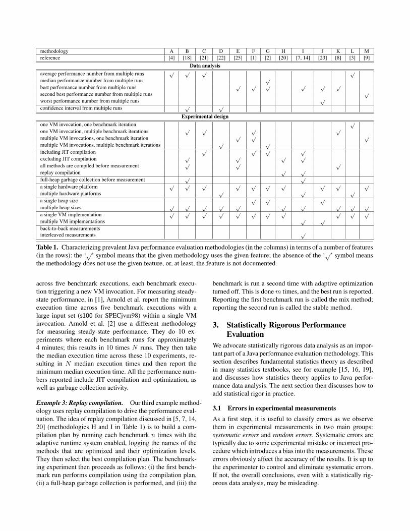
methodology A B C D E F G H I J K L Mreference [4] [18] [21] [22] [25] [1] [2] [20] [7, 14] [23] [8] [3] [9]
Data analysisaverage performance number from multiple runs √ √ √ √
median performance number from multiple runs √
best performance number from multiple runs √ √ √ √ √ √
second best performance number from multiple runs √
worst performance number from multiple runs √
confidence interval from multiple runs √ √
Experimental designone VM invocation, one benchmark iteration √
one VM invocation, multiple benchmark iterations √ √ √ √
multiple VM invocations, one benchmark iteration √ √ √
multiple VM invocations, multiple benchmark iterations √ √
including JIT compilation √ √ √ √
excluding JIT compilation √ √ √ √
all methods are compiled before measurement √ √ √
replay compilation √ √
full-heap garbage collection before measurement √ √
a single hardware platform √ √ √ √ √ √ √ √ √ √
multiple hardware platforms √ √ √
a single heap size √ √ √
multiple heap sizes √ √ √ √ √ √ √ √ √ √
a single VM implementation √ √ √ √ √ √ √ √ √ √ √
multiple VM implementations √ √
back-to-back measurementsinterleaved measurements √
Table 1. Characterizing prevalent Java performance evaluation methodologies (in the columns) in terms of a number of features(in the rows): the ‘√’ symbol means that the given methodology uses the given feature; the absence of the ‘√’ symbol meansthe methodology does not use the given feature, or, at least, the feature is not documented.
across five benchmark executions, each benchmark execu-tion triggering a new VM invocation. For measuring steady-state performance, in [1], Arnold et al. report the minimumexecution time across five benchmark executions with alarge input set (s100 for SPECjvm98) within a single VMinvocation. Arnold et al. [2] use a different methodologyfor measuring steady-state performance. They do 10 ex-periments where each benchmark runs for approximately4 minutes; this results in 10 times N runs. They then takethe median execution time across these 10 experiments, re-sulting in N median execution times and then report theminimum median execution time. All the performance num-bers reported include JIT compilation and optimization, aswell as garbage collection activity.
Example 3: Replay compilation. Our third example method-ology uses replay compilation to drive the performance eval-uation. The idea of replay compilation discussed in [5, 7, 14,20] (methodologies H and I in Table 1) is to build a com-pilation plan by running each benchmark n times with theadaptive runtime system enabled, logging the names of themethods that are optimized and their optimization levels.They then select the best compilation plan. The benchmark-ing experiment then proceeds as follows: (i) the first bench-mark run performs compilation using the compilation plan,(ii) a full-heap garbage collection is performed, and (iii) the
benchmark is run a second time with adaptive optimizationturned off. This is done m times, and the best run is reported.Reporting the first benchmark run is called the mix method;reporting the second run is called the stable method.
3. Statistically Rigorous PerformanceEvaluation
We advocate statistically rigorous data analysis as an impor-tant part of a Java performance evaluation methodology. Thissection describes fundamental statistics theory as describedin many statistics textbooks, see for example [15, 16, 19],and discusses how statistics theory applies to Java perfor-mance data analysis. The next section then discusses how toadd statistical rigor in practice.
3.1 Errors in experimental measurementsAs a first step, it is useful to classify errors as we observethem in experimental measurements in two main groups:systematic errors and random errors. Systematic errors aretypically due to some experimental mistake or incorrect pro-cedure which introduces a bias into the measurements. Theseerrors obviously affect the accuracy of the results. It is up tothe experimenter to control and eliminate systematic errors.If not, the overall conclusions, even with a statistically rig-orous data analysis, may be misleading.
Random errors, on the other hand, are unpredictable andnon-deterministic. They are unbiased in that a random er-ror may decrease or increase a measurement. There may bemany sources of random errors in the system. In practice, animportant concern is the presence of perturbing events thatare unrelated to what the experimenter is aiming at measur-ing, such as external system events, that cause outliers toappear in the measurements. Outliers need to be examinedclosely, and if the outliers are a result of a perturbing event,they should be discarded. Taking the best measurement alsoalleviates the issue with outliers, however, we advocate dis-carding outliers and applying statistically rigorous data anal-ysis to the remaining measurements.
While it is impossible to predict random errors, it ispossible to develop a statistical model to describe the overalleffect of random errors on the experimental results, whichwe do next.
3.2 Confidence intervals for the meanIn each experiment, a number of samples is taken from anunderlying population. A confidence interval for the meanderived from these samples then quantifies the range of val-ues that have a given probability of including the actual pop-ulation mean. While the way in which a confidence intervalis computed is essentially similar for all experiments, a dis-tinction needs to be made depending on the number of sam-ples gathered from the underlying population [16]: (i) thenumber of samples n is large (typically, n ≥ 30), and (ii) thenumber of samples n is small (typically, n < 30). We nowdiscuss both cases.
3.2.1 When the number of measurements is large(n ≥ 30)
Building a confidence interval requires that we have a num-ber of measurements xi, 1 ≤ i ≤ n, from a population withmean µ and variance σ2. The mean of these measurementsx is computed as
x =∑n
i=1 xi
n.
We will approximate the actual true value µ by the mean ofour measurements x and we will compute a range of val-ues [c1, c2] around x that defines the confidence interval ata given probability (called the confidence level). The con-fidence interval [c1, c2] is defined such that the probabilityof µ being between c1 and c2 equals 1 − α; α is called thesignificance level and (1− α) is called the confidence level.
Computing the confidence interval builds on the centrallimit theory. The central limit theory states that, for largevalues of n (typically n ≥ 30), x is approximately Gaussiandistributed with mean µ and standard deviation σ/
√n, pro-
vided that the samples xi, 1 ≤ i ≤ n, are (i) independent and(ii) come from the same population with mean µ and finitestandard deviation σ.
Because the significance level α is chosen a priori, weneed to determine c1 and c2 such that Pr[c1 ≤ µ ≤ c2] =
1 − α holds. Typically, c1 and c2 are chosen to form asymmetric interval around x, i.e., Pr[µ < c1] = Pr[µ >c2] = α/2. Applying the central-limit theorem, we find that
c1 = x− z1−α/2s√n
c2 = x + z1−α/2s√n
,
with x the sample mean, n the number of measurements ands the sample standard deviation computed as follows:
s =
√∑ni=1(xi − x)2
n− 1.
The value z1−α/2 is defined such that a random variable Zthat is Gaussian distributed with mean µ = 0 and varianceσ2 = 1, obeys the following property:
Pr[Z ≤ z1−α/2] = 1− α/2.
The value z1−α/2 is typically obtained from a precomputedtable.
3.2.2 When the number of measurements is small(n < 30)
A basic assumption made in the above derivation is that thesample variance s2 provides a good estimate of the actualvariance σ2. This assumption enabled us to approximate z =(x− µ)/(σ/
√n) as a standard normally distributed random
variable, and by consequence to compute the confidenceinterval for x. This is generally the case for experiments witha large number of samples, e.g., n ≥ 30.
However, for a relatively small number of samples, whichis typically assumed to mean n < 30, the sample variances2 can be significantly different from the actual variance σ2
of the underlying population [16]. In this case, it can beshown that the distribution of the transformed value t =(x − µ)/(s/
√n) follows the Student’s t-distribution with
n − 1 degrees of freedom. By consequence, the confidenceinterval can then be computed as:
c1 = x− t1−α/2;n−1s√n
c2 = x + t1−α/2;n−1s√n
,
with the value t1−α/2;n−1 defined such that a random vari-able T that follows the Student’s t distribution with n − 1degrees of freedom, obeys:
Pr[T ≤ t1−α/2;n−1] = 1− α/2.
The value t1−α/2;n−1 is typically obtained from a precom-puted table. It is interesting to note that as the number ofmeasurements n increases, the Student t-distribution ap-proaches the Gaussian distribution.
3.2.3 DiscussionInterpretation. In order to interpret experimental resultswith confidence intervals, we need to have a good under-standing of what a confidence interval actually means. A90% confidence interval, i.e., a confidence interval with a90% confidence level, means that there is a 90% probabilitythat the actual distribution mean of the underlying popula-tion, µ, is within the confidence interval. Increasing the con-fidence level to 95% means that we are increasing the prob-ability that the actual mean is within the confidence interval.Since we do not change our measurements, the only way toincrease the probability of the mean being within this newconfidence interval is to increase its size. By consequence,a 95% confidence interval will be larger than a 90% confi-dence interval; likewise, a 99% confidence interval will belarger than a 95% confidence interval.
Note on normality. It is also important to emphasize thatcomputing confidence intervals does not require that the un-derlying data is Gaussian or normally distributed. The cen-tral limit theory, which is at the foundation of the confidenceinterval computation, states that x is normally distributed ir-respective of the underlying distribution of the populationfrom which the measurements are taken. In other words,even if the population is not normally distributed, the av-erage measurement mean x is approximately Gaussian dis-tributed if the measurements are taken independently fromeach other.
3.3 Comparing two alternativesSo far, we were only concerned about computing the con-fidence interval for the mean of a single system. In termsof a Java performance evaluation setup, this is a single Javabenchmark with a given input running on a single virtualmachine with a given heap size running on a given hardwareplatform. However, in many practical situations, a researcheror benchmarker wants to compare the performance of two ormore systems. In this section, we focus on comparing twoalternatives; the next section then discusses comparing morethan two alternatives. A practical use case scenario could beto compare the performance of two virtual machines runningthe same benchmark with a given heap size on a given hard-ware platform. Another example use case is comparing theperformance of two garbage collectors for a given bench-mark, heap size and virtual machine on a given hardwareplatform.
The simplest approach to comparing two alternatives is todetermine whether the confidence intervals for the two setsof measurements overlap. If they do overlap, then we cannotconclude that the differences seen in the mean values arenot due to random fluctuations in the measurements. In otherwords, the difference seen in the mean values is possibly dueto random effects. If the confidence intervals do not overlap,however, we conclude that there is no evidence to suggestthat there is not a statistically significant difference. Note
the careful wording here. There is still a probability α thatthe differences observed in our measurements are simply dueto random effects in our measurements. In other words, wecannot assure with a 100% certainty that there is an actualdifference between the compared alternatives. In some cases,taking such ‘weak’ conclusions may not be very satisfying— people tend to like strong and affirmative conclusions —but it is the best we can do given the statistical nature of themeasurements.
Consider now two alternatives with n1 measurementsof the first alternative and n2 measurements of the secondalternative. We then first determine the sample means x1
and x2 and the sample standard deviations s1 and s2. Wesubsequently compute the difference of the means as x =x1 − x2. The standard deviation sx of this difference of themean values is then computed as:
sx =
√s21
n1+
s22
n2.
The confidence interval for the difference of the means isthen given by
c1 = x− z1−α/2sx
c2 = x + z1−α/2sx.
If this confidence interval includes zero, we can conclude,at the confidence level chosen, that there is no statisticallysignificant difference between the two alternatives.
The above only holds in case the number of measure-ments is large on both systems, i.e., n1 ≥ 30 and n2 ≥ 30. Incase the number of measurements on at least one of the twosystems is smaller than 30, then we can no longer assumethat the difference of the means is normally distributed. Wethen need to resort to the Student’s t distribution by replac-ing the value z1−α/2 in the above formula with t1−α/2;ndf
;the degrees of freedom ndf is then to be approximated by theinteger number nearest to
ndf =
(s21
n1+ s2
2n2
)2
(s21/n1)2
n1−1 + (s22/n2)2
n2−1
.
3.4 Comparing more than two alternatives: ANOVAThe approach discussed in the previous section to compar-ing two alternatives is simple and intuitively appealing, how-ever, it is limited to comparing two alternatives. A more gen-eral and more robust technique is called Analysis of Vari-ance (ANOVA). ANOVA separates the total variation in a setof measurements into a component due to random fluctua-tions in the measurements and a component due to the actualdifferences among the alternatives. In other words, ANOVAseparates the total variation observed in (i) the variation ob-served within each alternative, which is assumed to be aresult of random effects in the measurements, and (ii) thevariation between the alternatives. If the variation between
the alternatives is larger than the variation within each alter-native, then it can be concluded that there is a statisticallysignificant difference between the alternatives. ANOVA as-sumes that the variance in measurement error is the samefor all of the alternatives. Also, ANOVA assumes that theerrors in the measurements for the different alternatives areindependent and Gaussian distributed. However, ANOVA isfairly robust towards non-normality, especially in case thereis a balanced number of measurements for each of the alter-natives.
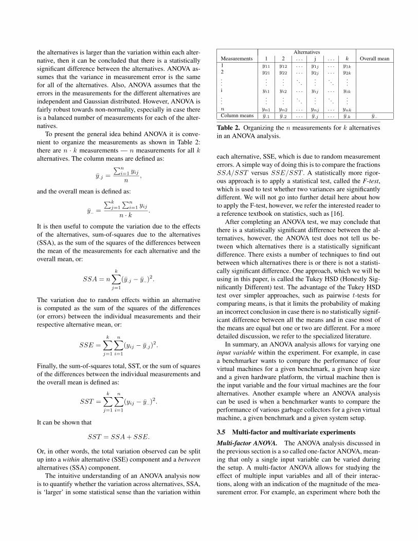
To present the general idea behind ANOVA it is conve-nient to organize the measurements as shown in Table 2:there are n · k measurements — n measurements for all kalternatives. The column means are defined as:
y.j =∑n
i=1 yij
n,
and the overall mean is defined as:
y.. =
∑kj=1
∑ni=1 yij
n · k.
It is then useful to compute the variation due to the effectsof the alternatives, sum-of-squares due to the alternatives(SSA), as the sum of the squares of the differences betweenthe mean of the measurements for each alternative and theoverall mean, or:
SSA = n
k∑j=1
(y.j − y..)2.
The variation due to random effects within an alternativeis computed as the sum of the squares of the differences(or errors) between the individual measurements and theirrespective alternative mean, or:
SSE =k∑
j=1
n∑i=1
(yij − y.j)2.
Finally, the sum-of-squares total, SST, or the sum of squaresof the differences between the individual measurements andthe overall mean is defined as:
SST =k∑
j=1
n∑i=1
(yij − y..)2.
It can be shown that
SST = SSA + SSE.
Or, in other words, the total variation observed can be splitup into a within alternative (SSE) component and a betweenalternatives (SSA) component.
The intuitive understanding of an ANOVA analysis nowis to quantify whether the variation across alternatives, SSA,is ‘larger’ in some statistical sense than the variation within
AlternativesMeasurements 1 2 . . . j . . . k Overall mean1 y11 y12 . . . y1j . . . y1k
2 y21 y22 . . . y2j . . . y2k
......
.... . .
.... . .
...i yi1 yi2 . . . yij . . . yik
......
.... . .
.... . .
...n yn1 yn2 . . . ynj . . . ynk
Column means y.1 y.2 . . . y.j . . . y.k y..
Table 2. Organizing the n measurements for k alternativesin an ANOVA analysis.
each alternative, SSE, which is due to random measurementerrors. A simple way of doing this is to compare the fractionsSSA/SST versus SSE/SST . A statistically more rigor-ous approach is to apply a statistical test, called the F-test,which is used to test whether two variances are significantlydifferent. We will not go into further detail here about howto apply the F-test, however, we refer the interested reader toa reference textbook on statistics, such as [16].
After completing an ANOVA test, we may conclude thatthere is a statistically significant difference between the al-ternatives, however, the ANOVA test does not tell us be-tween which alternatives there is a statistically significantdifference. There exists a number of techniques to find outbetween which alternatives there is or there is not a statisti-cally significant difference. One approach, which we will beusing in this paper, is called the Tukey HSD (Honestly Sig-nificantly Different) test. The advantage of the Tukey HSDtest over simpler approaches, such as pairwise t-tests forcomparing means, is that it limits the probability of makingan incorrect conclusion in case there is no statistically signif-icant difference between all the means and in case most ofthe means are equal but one or two are different. For a moredetailed discussion, we refer to the specialized literature.
In summary, an ANOVA analysis allows for varying oneinput variable within the experiment. For example, in casea benchmarker wants to compare the performance of fourvirtual machines for a given benchmark, a given heap sizeand a given hardware platform, the virtual machine then isthe input variable and the four virtual machines are the fouralternatives. Another example where an ANOVA analysiscan be used is when a benchmarker wants to compare theperformance of various garbage collectors for a given virtualmachine, a given benchmark and a given system setup.
3.5 Multi-factor and multivariate experimentsMulti-factor ANOVA. The ANOVA analysis discussed inthe previous section is a so called one-factor ANOVA, mean-ing that only a single input variable can be varied duringthe setup. A multi-factor ANOVA allows for studying theeffect of multiple input variables and all of their interac-tions, along with an indication of the magnitude of the mea-surement error. For example, an experiment where both the
garbage collector and the heap size are varied, could providedeep insight into the effect on overall performance of boththe garbage collector and the heap size individually as wellas the interaction of both the garbage collector and the heapsize.
Multivariate ANOVA. The ANOVA analyses discussed sofar only consider, what is called, a single dependent vari-able. In a Java context, this means that an ANOVA analysisonly allows for making conclusions about a single bench-mark. However, a benchmarker typically considers a num-ber of benchmarks and is interested in the performance forall the benchmarks — it is important for a performance eval-uation study to consider a large enough set of representativebenchmarks. A multivariate ANOVA (MANOVA) allows forconsidering multiple dependent variables, or multiple bench-marks, within one single experiment. The key point of per-forming a MANOVA instead of multiple ANOVA analyseson the individual dependent variables, is that a MANOVAanalysis takes into account the correlation across the depen-dent variables whereas multiple ANOVAs do not.
3.6 DiscussionIn the previous sections, we explored a wide range of statis-tical techniques and we discussed how to apply these tech-niques within a Java performance evaluation context. How-ever, using the more complex analyses, such as multi-factorANOVA and MANOVA, raises two concerns. First, theiroutput is often non-intuitive and in many cases hard to un-derstand without deep background knowledge in statistics.Second, as mentioned before, doing all the measurements re-quired as input to the analyses can be very time-consuming,up to the point where it becomes intractable. For these rea-sons, we limit ourselves to a Java performance evaluationmethodology that is practical yet statistically rigorous. Themethodology that we present computes confidence intervalswhich allows for doing comparisons between alternatives ona per-benchmark basis, as discussed in sections 3.3 and 3.4.Of course, a benchmarker who is knowledgeable in statisticsmay perform more complex analyses.
4. A practical statistically rigorousmethodology
Having discussed the general theory of statistics and howit relates to Java performance evaluation, we suggest morepractical and statistically rigorous methodologies for quan-tifying startup and steady-state Java performance by com-bining a number of existing approaches. The evaluation sec-tion in this paper then compares the accuracy of prevalentdata analysis methodologies against these statistically rigor-ous methodologies.
Notation. We refer to xij as the measurement of the j-thbenchmark iteration of the i-th VM invocation.
4.1 Startup performanceThe goal of measuring start-up performance is to measurehow quickly a Java virtual machine can execute a relativelyshort-running Java program. There are two key differencesbetween startup and steady-state performance. First, startupperformance includes class loading whereas steady-stateperformance does not, and, second, startup performance isaffected by JIT compilation, substantially more than steady-state performance.
For measuring startup performance, we advocate a two-step methodology:
1. Measure the execution time of multiple VM invocations,each VM invocation running a single benchmark itera-tion. This results in p measurements xij with 1 ≤ i ≤ pand j = 1.
2. Compute the confidence interval for a given confidencelevel as described in Section 3.2. If there are more than30 measurements, use the standard normal z-statistic;otherwise use the Student t-statistic.
Recall that the central limit theory assumes that the mea-surements are independent. This may not be true in prac-tice, because the first VM invocation in a series of measure-ments may change system state that persists past this firstVM invocation, such as dynamically loaded libraries persist-ing in physical memory or data persisting in the disk cache.To reach independence, we discard the first VM invocationfor each benchmark from our measurements and only retainthe subsequent measurements, as done by several other re-searchers; this assumes that the libraries are loaded whendoing the measurements.
4.2 Steady-state performanceSteady-state performance concerns long-running applica-tions for which start-up is of less interest, i.e., the appli-cation’s total running time largely exceeds start-up time.Since most of the JIT compilation is performed during start-up, steady-state performance suffers less from variabilitydue to JIT compilation. However, the other sources of non-determinism, such as thread scheduling and system effects,still remain under steady-state, and thus need to be consid-ered.
There are two issues with quantifying steady-state per-formance. The first issue is to determine when steady-stateperformance is reached. Long-running applications typicallyrun on large or streaming input data sets. Benchmarkers typ-ically approximate long-running benchmarks by running ex-isting benchmarks with short inputs multiple times within asingle VM invocation, i.e., the benchmark is iterated multi-ple times. The question then is how many benchmark iter-ations do we need to consider before we reach steady-stateperformance within a single VM invocation? This is a dif-ficult question to answer in general; the answer will differ
from application to application, and in some cases it maytake a very long time before steady-state is reached.
The second issue with steady-state performance is thatdifferent VM invocations running multiple benchmark iter-ations may result in different steady-state performances [2].Different methods may be optimized at different levels ofoptimization across different VM invocations, changingsteady-state performance.
To address these two issues, we advocate a four-stepmethodology for quantifying steady-state performance:
1. Consider p VM invocations, each VM invocation runningat most q benchmark iterations. Suppose that we want toretain k measurements per invocation.
2. For each VM invocation i, determine the iteration si
where steady-state performance is reached, i.e., once thecoefficient of variation (CoV)1 of the k iterations (si − kto si) falls below a preset threshold, say 0.01 or 0.02.
3. For each VM invocation, compute the mean xi of the kbenchmark iterations under steady-state:
xi =si∑
j=si−k
xij .
4. Compute the confidence interval for a given confidencelevel across the computed means from the different VMinvocations. The overall mean equals x =
∑pi=1 xi, and
the confidence interval is computed over the xi measure-ments.
We thus first compute the mean xi across multiple iter-ations within a single VM invocation i, and subsequentlycompute the confidence interval across the p VM invoca-tions using the xi means, see steps 3 and 4 from above. Thereason for doing so is to reach independence across the mea-surements from which we compute the confidence interval:the various iterations within a single VM invocation are notindependent, however, the mean values xi across multipleVM invocations are independent.
4.3 In practiceTo facilitate the application of these start-up and steady-stateperformance evaluation methodologies, we provide publiclyavailable software called JavaStats 2 that readily works withthe SPECjvm98 and DaCapo benchmark suites. For startupperformance, a script (i) triggers multiple VM invocationsrunning a single benchmark iteration, (ii) monitors the exe-cution time of each invocation, and (iii) computes the confi-dence interval for a given confidence level. If the confidenceinterval achieves a desired level of precision, i.e., the confi-dence interval is within 1% or 2% of the sample mean, thescript stops the experiment, and reports the sample mean and
1 CoV is defined as the standard deviation s divided by the mean x.2 Available at http://www.elis.UGent.be/JavaStats/.
its confidence interval. Or, if the desired level of precision isnot reached after a preset number of runs, e.g., 30 runs, theobtained confidence interval is simply reported along withthe sample mean.
For steady-state performance, JavaStats collects execu-tion times across multiple VM invocations and across mul-tiple benchmark iterations within a single VM invocation.JavaStats consists of a script running multiple VM invoca-tions as well as a benchmark harness triggering multiple iter-ations within a single VM invocation. The output for steady-state performance is similar to what is reported above forstartup performance.
SPECjvm98 as well as the DaCapo benchmark suite al-ready come with a harness to set the desired number ofbenchmark iterations within a single VM invocation. Thecurrent version of the DaCapo harness also determines howmany iterations are needed to achieve a desired level of co-efficient of variation (CoV). As soon as the observed CoVdrops below a given threshold (the convergence target) for agiven window of iterations, the execution time for the next it-eration is reported. JavaStats extends the existing harnesses(i) by enabling measurements across multiple VM invoca-tions instead of a single VM invocation, and (ii) by comput-ing and reporting confidence intervals.
These Java performance analysis methodologies do notcontrol non-determinism. However, a statistically rigorousdata analysis approach can also be applied together with anexperimental design that controls the non-determinism, suchas replay compilation. Confidence intervals can be used toquantify the remaining random fluctuations in the systemunder measurement.
A final note that we would like to make is that collectingthe measurements for a statistically rigorous data analysiscan be time-consuming, especially if the experiment needs alarge number of VM invocations and multiple benchmarkiterations per VM invocation (in case of steady-state per-formance). Under time pressure, statistically rigorous dataanalysis can still be applied considering a limited numberof measurements, however, the confidence intervals will belooser.
5. Experimental SetupThe next section will evaluate prevalent data analysis ap-proaches against statistically rigorous data analysis. For do-ing so, we consider an experiment in which we compare var-ious garbage collection (GC) strategies — similar to what isbeing done in the GC research literature. This section dis-cusses the experimental setup: the virtual machine configu-rations, the benchmarks and the hardware platforms.
5.1 Virtual machine and GC strategiesWe use the Jikes Research Virtual Machine (RVM) [1] whichis an open source Java virtual machine written in Java. JikesRVM employs baseline compilation to compile a method
upon its first execution; hot methods are sampled by an OS-triggered sampling mechanism and subsequently scheduledfor further optimization. There are three optimization levelsin Jikes RVM: 0, 1 and 2. We use the February 12, 2007 SVNversion of Jikes RVM in all of our experiments.
We consider five garbage collection strategies in to-tal, all implemented in the Memory Management Toolkit(MMTk) [6], the garbage collection toolkit provided withthe Jikes RVM. The five garbage collection strategies are: (i)CopyMS, (ii) GenCopy, (iii) GenMS, (iv) MarkSweep, and(v) SemiSpace; the generational collectors use a variable-size nursery. GC poses a complex space-time trade-off, andit is unclear which GC strategy is the winner without doinga detailed experimentation. We did not include the GenRC,MarkCompact and RefCount collectors from MMTk, be-cause we were unable to successfully run Jikes with theGenRC and MarkCompact collector for some of the bench-marks; and RefCount did yield performance numbers thatare statistically significantly worse than any other GC strat-egy across all benchmarks.
5.2 BenchmarksTable 3 shows the benchmarks used in this study. We usethe SPECjvm98 benchmarks [23] (first seven rows), aswell as seven DaCapo benchmarks [7] (next seven rows).SPECjvm98 is a client-side Java benchmark suite consistingof seven benchmarks. We run all SPECjvm98 benchmarkswith the largest input set (-s100). The DaCapo benchmarkis a recently introduced open-source benchmark suite; weuse release version 2006-10-MR2. We use the seven bench-marks that execute properly on the February 12, 2007 SVNversion of Jikes RVM. We use the default (medium size)input set for the DaCapo benchmarks.
In all of our experiments, we consider a per-benchmarkheap size range, following [5]. We vary the heap size froma minimum heap size up to 6 times this minimum heap size,in steps of 0.25 times the minimum heap size. The per-benchmark minimum heap sizes are shown in Table 3.
5.3 Hardware platformsFollowing the advice by Blackburn et al. [7], we considermultiple hardware platforms in our performance evaluationmethodology: a 2.1GHz AMD Athlon XP, a 2.8GHz IntelPentium 4, and a 1.42GHz Mac PowerPC G4 machine. TheAMD Athlon and Intel Pentium 4 have 2GB of main mem-ory; the Mac PowerPC G4 has 1GB of main memory. Thesemachines run the Linux operating system, version 2.6.18. Inall of our experiments we consider an otherwise idle and un-loaded machine.
6. EvaluationWe now evaluate the proposed statistically rigorous Javaperformance data analysis methodology in three steps. Wefirst measure Java program run-time variability. In a second
benchmark description min heapsize (MB)
compress file compression 24jess puzzle solving 32db database 32javac Java compiler 32mpegaudio MPEG decompression 16mtrt raytracing 32jack parsing 24antlr parsing 32bloat Java bytecode optimization 56fop PDF generation from XSL-FO 56hsqldb database 176jython Python interpreter 72luindex document indexing 32pmd Java class analysis 64
Table 3. SPECjvm98 (top seven) and DaCapo (bottomseven) benchmarks considered in this paper. The rightmostcolumn indicates the minimum heap size, as a multiple of8MB, for which all GC strategies run to completion.
0.95
1.00
1.05
com
pres
s
jess db
java
c
mpe
gaud
io
mtr
t
jack
antlr
bloa
t
fop
hsql
db
jyth
on
luin
dex
pmd
● ●●
●●
● ●● ● ● ●
●● ●
Nor
mal
ized
exe
cutio
n tim
e
Figure 2. Run-time variability normalized to the mean exe-cution time for start-up performance. These experiments as-sume 30 VM invocations on the AMD Athlon platform withthe GenMS collector and a per-benchmark heap size that istwice as large as the minimal heap size reported in Table 3.The dot represents the median.
step, we compare prevalent methods from Section 2 againstthe statistically rigorous method from Section 3. And as afinal step, we demonstrate the use of the software providedto perform a statistically rigorous performance evaluation.
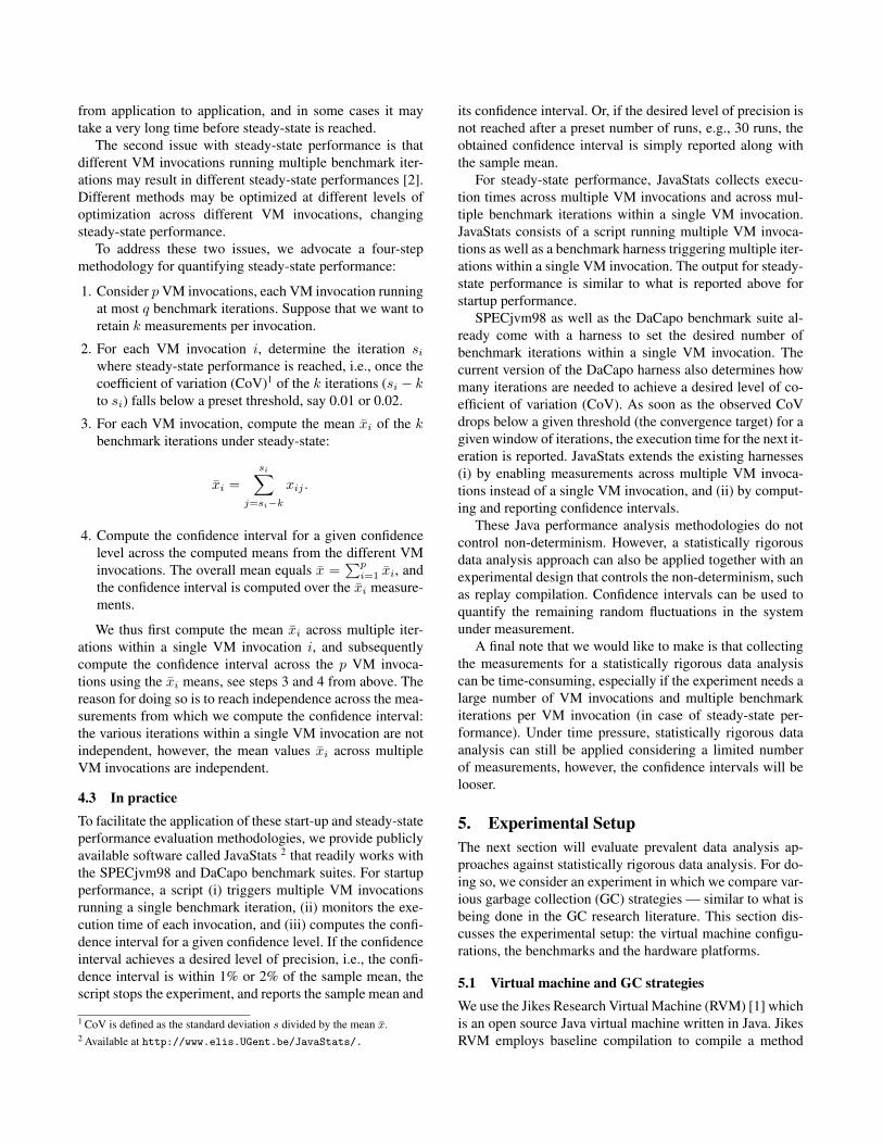
6.1 Run-time variabilityThe basic motivation for this work is that running a Javaprogram introduces run-time variability caused by non-determinism. Figure 2 demonstrates this run-time variabilityfor start-up performance, and Figure 3 shows the same for
0.9
1.0
1.1
1.2
1.3
1.4co
mpr
ess
jess db
java
c
mpe
gaud
io
mtr
t
jack
bloa
t
fop
hsql
db
jyth
on
luin
dex
pmd
●●
●
●
●
● ●●
● ●● ●
●Nor
mal
ized
exe
cutio
n tim
e
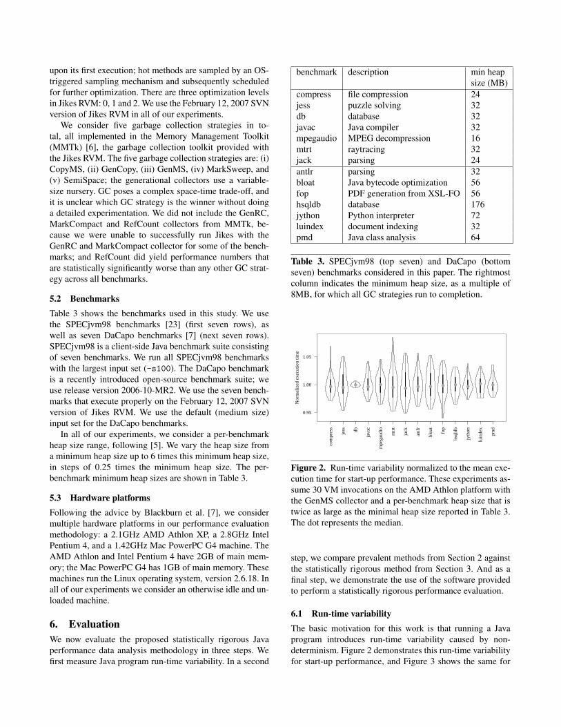
Figure 3. Run-time variability normalized to the mean ex-ecution time for steady-state performance. These experi-ments assume 10 VM invocations and 30 benchmark iter-ations per VM invocation on the AMD Athlon platform withthe GenMS collector and a per-benchmark heap size that istwice as large as the minimal heap size reported in Table 3.The dot represents the median.
steady-state performance3. This experiment assumes 30 VMinvocations (and a single benchmark iteration) for start-upperformance and 10 VM invocations and 30 benchmark it-erations per VM invocation for steady-state performance.These graphs show violin plots [13]4; all values are nor-malized to a mean of one. A violin plot is very similar toa box plot. The middle point shows the median; the thickvertical line represents the first and third quartile (50% ofall the data points are between the first and third quartile);the thin vertical line represents the upper and lower adjacentvalues (representing an extreme data point or 1.5 times theinterquartile range from the median, whichever comes first);and the top and bottom values show the maximum and min-imum values. The important difference with a box plot isthat the shape of the violin plot represents the density: thewider the violin plot, the higher the density. In other words,a violin plot visualizes a distribution’s probability densityfunction whereas a box plot does not.
There are a couple of interesting observations to be madefrom these graphs. First, run-time variability can be fairlysignificant, for both startup and steady-state performance.For most of the benchmarks, the coefficient of variation(CoV), defined as the standard deviation divided by themean, is around 2% and is higher for several benchmarks.Second, the maximum performance difference between themaximum and minimum performance number varies acrossthe benchmarks, and is generally around 8% for startup and20% for steady-state. Third, most of the violin plots in Fig-
3 The antlr benchmark does not appear in Figure 3 because we were unableto run more than a few iterations within a single VM invocation.4 The graphs shown were made using R – a freely available statisticalframework – using the vioplot package available from the CRAN (at http://www.r-project.org).
ures 2 and 3 show that the measurement data is approxi-mately Gaussian distributed with the bulk weight around themean. Statistical analyses, such as the Kolmogorov-Smirnovtest, do not reject the hypothesis that in most of our measure-ments the data is approximately Gaussian distributed — infact, this is the case for more than 90% of the experimentsdone in this paper involving multiple hardware platforms,benchmarks, GC strategies and heap sizes. However, in aminority of the measurements we observe non-Gaussiandistributed data; some of these have skewed distributionsor bimodal distributions. Note however that a non-Gaussiandistribution does not affect the generality of the proposedstatistically rigorous data analysis technique. As discussedin section 3.2.3, the central limit theory does not assume themeasurement data to be Gaussian distributed; also, ANOVAis robust towards non-normality.
6.2 Evaluating prevalent methodologiesWe now compare the prevalent data analysis methodologiesagainst the statistically rigorous data analysis approach ad-vocated in this paper. For doing so, we set up an experimentin which we (pairwise) compare the overall performance ofvarious garbage collectors over a range of heap sizes. Weconsider the various GC strategies as outlined in section 5,a range of heap sizes from the minimum heap size up to sixtimes this minimum heap size in 0.25 minimum heap sizeincrements — there are 21 heap sizes in total. Computingconfidence intervals for the statistically rigorous methodol-ogy is done, following section 3, by applying an ANOVAand a Tukey HSD test to compute simultaneous 95% confi-dence intervals for all the GC strategies per benchmark andper heap size.
To evaluate the accuracy of the prevalent performanceevaluation methodologies we consider all possible pairwiseGC strategy comparisons for all heap sizes considered. Foreach heap size, we then determine whether prevalent dataanalysis leads to the same conclusion as statistically rigorousdata analysis. In other words, there are C2
5 = 10 pairwise GCcomparisons per heap size and per benchmark. Or, 210 GCcomparisons in total across all heap sizes per benchmark.
We now classify all of these comparisons in six cate-gories, see Table 4, and then report the relative frequency ofeach of these six categories. These results help us better un-derstand the frequency of misleading and incorrect conclu-sions using prevalent performance methodologies. We makea distinction between overlapping confidence intervals andnon-overlapping confidence intervals, according to the sta-tistically rigorous methodology.
Overlapping confidence intervals. Overlapping confidenceintervals indicate that the performance differences observedmay be due to random fluctuations. As a result, any con-clusion taken by a methodology that concludes that one al-ternative performs better than another is questionable. Theonly valid conclusion with overlapping confidence intervals
prevalent methodologyperformance difference < θ performance difference ≥ θ
statistically rigorous methodologyoverlapping intervals indicative misleading
non-overlapping intervals, same order misleading but correct correctnon-overlapping intervals, not same order misleading and incorrect incorrect
Table 4. Classifying conclusions by a prevalent methodology in comparison to a statistically rigorous methodology.
is that there is no statistically significant difference betweenthe alternatives.
Performance analysis typically does not state that one al-ternative is better than another when the performance dif-ference is very small though. To mimic this practice, we in-troduce a threshold θ to classify decisions: a performancedifference smaller than θ is considered a small performancedifference and a performance difference larger than θ is con-sidered a large performance difference. We vary the θ thresh-old from 1% up to 3%.
Now, in case the performance difference by the prevalentmethodology is considered large, we conclude the prevalentmethodology to be ‘misleading’. In other words, the preva-lent methodology says there is a significant performance dif-ference whereas the statistics conclude that this performancedifference may be due to random fluctuations. If the perfor-mance difference is small based on the prevalent methodol-ogy, we consider the prevalent methodology to be ‘indica-tive’.
Non-overlapping confidence intervals. Non-overlappingconfidence intervals suggest that we can conclude thatthere are statistically significant performance differencesamong the alternatives. There are two possibilities for non-overlapping confidence intervals. If the ranking by the statis-tically rigorous methodology is the same as the ranking bythe prevalent methodology, then the prevalent methodologyis considered correct. If the methodologies have oppositerankings, then the prevalent methodology is considered tobe incorrect.
To incorporate a performance analyst’s subjective judge-ment, modeled through the θ threshold from above, we makeone more distinction based on whether the performance dif-ference is considered small or large. In particular, if theprevalent methodology states there is a small difference, theconclusion is classified to be misleading. In fact, there is astatistically significant performance difference, however, theperformance difference is small.
We have four classification categories for non-overlappingconfidence intervals, see Table 4. If the performance differ-ence by the prevalent methodology is larger than θ, and theranking by the prevalent methodology equals the rankingby the statistically rigorous methodology, then the prevalentmethodology is considered to be ‘correct’; if the prevalentmethodology has the opposite ranking as the statisticallyrigorous methodology, the prevalent methodology is consid-ered ‘incorrect’. In case of a small performance differenceaccording to the prevalent methodology, and the same rank-
ing as the statistically rigorous methodology, the prevalentmethodology is considered to be ‘misleading but correct’;in case of an opposite ranking, the prevalent methodology isconsidered ‘misleading and incorrect’.
6.2.1 Start-up performanceWe first focus on start-up performance. For now, we limitourselves to prevalent methodologies that do not use replaycompilation. We treat steady-state performance and replaycompilation in subsequent sections.
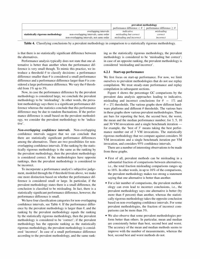
Figure 4 shows the percentage GC comparisons by theprevalent data analysis approaches leading to indicative,misleading and incorrect conclusions for θ = 1% andθ = 2% thresholds. The various graphs show different hard-ware platforms and different θ thresholds. The various barsin these graphs show various prevalent methodologies. Thereare bars for reporting the best, the second best, the worst,the mean and the median performance number; for 3, 5, 10and 30 VM invocations and a single benchmark iteration —for example, the ‘best of 3’ means taking the best perfor-mance number out of 3 VM invocations. The statisticallyrigorous methodology that we compare against considers 30VM invocations and a single benchmark iteration per VMinvocation, and considers 95% confidence intervals.
There are a number of interesting observations to be madefrom these graphs.
• First of all, prevalent methods can be misleading in asubstantial fraction of comparisons between alternatives,i.e., the total fraction misleading comparisons ranges upto 16%. In other words, in up to 16% of the comparisons,the prevalent methodology makes too strong a statementsaying that one alternative is better than another.
• For a fair number of comparisons, the prevalent method-ology can even lead to incorrect conclusions, i.e., theprevalent methodology says one alternative is better (bymore than θ percent) than another, whereas the statisti-cally rigorous methodology takes the opposite conclusionbased on non-overlapping confidence intervals. For someprevalent methodologies, the fraction of incorrect com-parisons can be more than 3%.
• We also observe that some prevalent methodologies per-form better than others. In particular, mean and medianare consistently better than best, second best and worst.The accuracy of the mean and median methods seems toimprove with the number of measurements, whereas thebest, second best and worst methods do not.
(a) AMD Athlon – θ = 1% (b) AMD Athlon – θ = 2%
05
1015202530
best
of 3
mea
n of 3
med
ian of
3se
cond
_bes
t of 3
worst
of 3
best
of 5
mea
n of 5
med
ian of
5se
cond
_bes
t of 5
worst
of 5
best
of 10
mea
n of 1
0m
edian
of 10
seco
nd_b
est o
f 10
worst
of 10
best
of 30
mea
n of 3
0m
edian
of 30
seco
nd_b
est o
f 30
worst
of 30pe
rcen
tage
of t
otal
com
paris
ons incorrect misleading misleading and incorrect misleading but correct indicative
(c) Intel Pentium 4 – θ = 1% (d) Intel Pentium 4 – θ = 2%
05
1015202530
best
of 3
mea
n of 3
med
ian of
3se
cond
_bes
t of 3
worst
of 3
best
of 5
mea
n of 5
med
ian of
5se
cond
_bes
t of 5
worst
of 5
best
of 10
mea
n of 1
0m
edian
of 10
seco
nd_b
est o
f 10
worst
of 10
best
of 30
mea
n of 3
0m
edian
of 30
seco
nd_b
est o
f 30
worst
of 30pe
rcen
tage
of t
otal
com
paris
ons incorrect misleading misleading and incorrect misleading but correct indicative
(e) PowerPC G4 – θ = 1% (f) PowerPC G4 – θ = 2%
05
1015202530
best
of 3
mea
n of 3
med
ian of
3se
cond
_bes
t of 3
worst
of 3
best
of 5
mea
n of 5
med
ian of
5se
cond
_bes
t of 5
worst
of 5
best
of 10
mea
n of 1
0m
edian
of 10
seco
nd_b
est o
f 10
worst
of 10
best
of 30
mea
n of 3
0m
edian
of 30
seco
nd_b
est o
f 30
worst
of 30pe
rcen
tage
of t
otal
com
paris
ons incorrect misleading misleading and incorrect misleading but correct indicative
Figure 4. Percentage GC comparisons by prevalent data analysis approaches leading to incorrect, misleading or indicativeconclusions. Results are shown for the AMD Athlon machine with θ = 1% (a) and θ = 2% (b), for the Intel Pentium 4machine with θ = 1% (c) and θ = 2% (d), and for the PowerPC G4 with θ = 1% (e) and θ = 2% (f).
θ-threshold
0
10
20
30
40
50
60
70
0
0.25 0.5 0.75 1
1.25 1.5 1.75 2
2.25 2.5 2.75 3
Perc
enta
ge o
f tot
al c
ompa
rison
s
incorrect misleading misleading and incorrect misleading but correct indicative
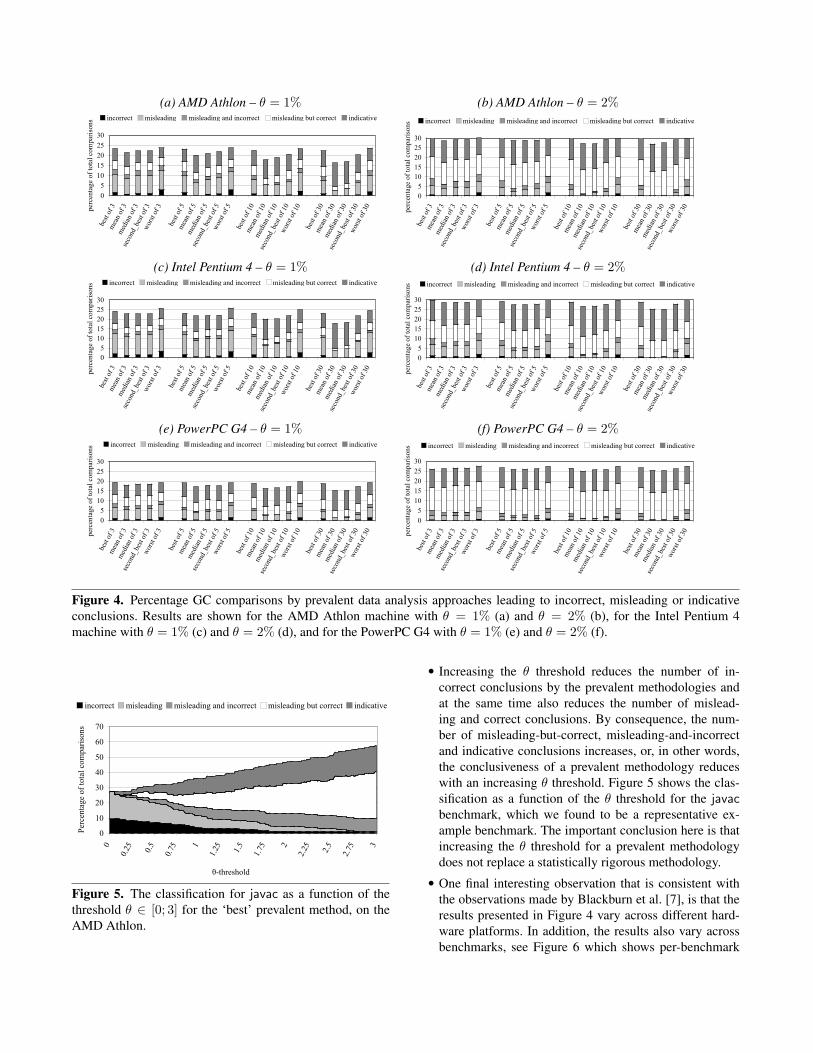
Figure 5. The classification for javac as a function of thethreshold θ ∈ [0; 3] for the ‘best’ prevalent method, on theAMD Athlon.
• Increasing the θ threshold reduces the number of in-correct conclusions by the prevalent methodologies andat the same time also reduces the number of mislead-ing and correct conclusions. By consequence, the num-ber of misleading-but-correct, misleading-and-incorrectand indicative conclusions increases, or, in other words,the conclusiveness of a prevalent methodology reduceswith an increasing θ threshold. Figure 5 shows the clas-sification as a function of the θ threshold for the javacbenchmark, which we found to be a representative ex-ample benchmark. The important conclusion here is thatincreasing the θ threshold for a prevalent methodologydoes not replace a statistically rigorous methodology.
• One final interesting observation that is consistent withthe observations made by Blackburn et al. [7], is that theresults presented in Figure 4 vary across different hard-ware platforms. In addition, the results also vary acrossbenchmarks, see Figure 6 which shows per-benchmark
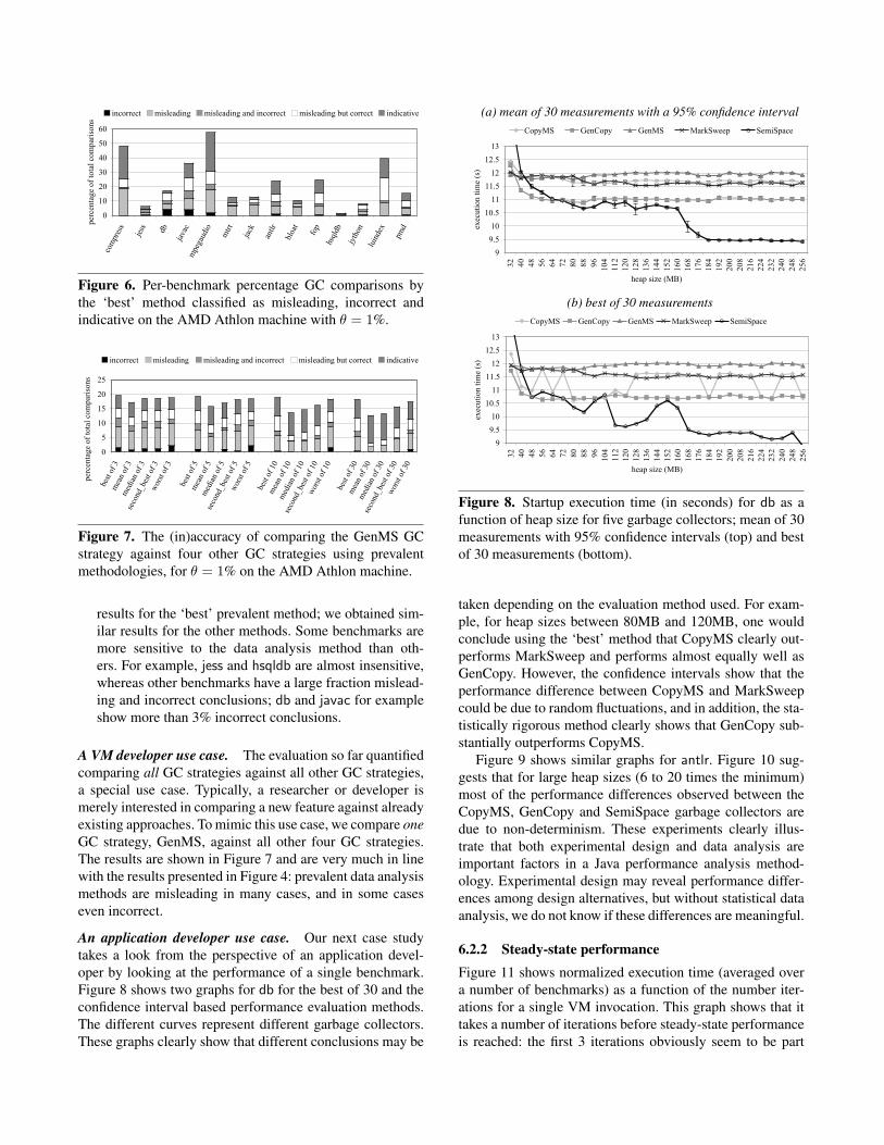
0
10
20
30
40
50
60
com
pres
s
jess db
javac
mpe
gaud
io
mtrt
jack
antlr
bloa
t
fop
hsql
dbjy
thon
luin
dex
pmdpe
rcen
tage
of t
otal
com
paris
ons
incorrect misleading misleading and incorrect misleading but correct indicative
Figure 6. Per-benchmark percentage GC comparisons bythe ‘best’ method classified as misleading, incorrect andindicative on the AMD Athlon machine with θ = 1%.
0
5
10
15
20
25
best
of 3
mea
n of 3
med
ian of
3se
cond
_bes
t of 3
worst
of 3
best
of 5
mea
n of 5
med
ian of
5se
cond
_bes
t of 5
worst
of 5
best
of 10
mea
n of 1
0m
edian
of 10
seco
nd_b
est o
f 10
worst
of 10
best
of 30
mea
n of 3
0m
edian
of 30
seco
nd_b
est o
f 30
worst
of 30
perc
enta
ge o
f tot
al c
ompa
rison
s
incorrect misleading misleading and incorrect misleading but correct indicative
Figure 7. The (in)accuracy of comparing the GenMS GCstrategy against four other GC strategies using prevalentmethodologies, for θ = 1% on the AMD Athlon machine.
results for the ‘best’ prevalent method; we obtained sim-ilar results for the other methods. Some benchmarks aremore sensitive to the data analysis method than oth-ers. For example, jess and hsqldb are almost insensitive,whereas other benchmarks have a large fraction mislead-ing and incorrect conclusions; db and javac for exampleshow more than 3% incorrect conclusions.
A VM developer use case. The evaluation so far quantifiedcomparing all GC strategies against all other GC strategies,a special use case. Typically, a researcher or developer ismerely interested in comparing a new feature against alreadyexisting approaches. To mimic this use case, we compare oneGC strategy, GenMS, against all other four GC strategies.The results are shown in Figure 7 and are very much in linewith the results presented in Figure 4: prevalent data analysismethods are misleading in many cases, and in some caseseven incorrect.
An application developer use case. Our next case studytakes a look from the perspective of an application devel-oper by looking at the performance of a single benchmark.Figure 8 shows two graphs for db for the best of 30 and theconfidence interval based performance evaluation methods.The different curves represent different garbage collectors.These graphs clearly show that different conclusions may be
(a) mean of 30 measurements with a 95% confidence interval
99.510
10.511
11.512
12.513
32 40 48 56 64 72 80 88 96 104
112
120
128
136
144
152
160
168
176
184
192
200
208
216
224
232
240
248
256
heap size (MB)
exec
utio
n tim
e (s
)
CopyMS GenCopy GenMS MarkSweep SemiSpace
(b) best of 30 measurements
99.510
10.511
11.512
12.513
32 40 48 56 64 72 80 88 96 104
112
120
128
136
144
152
160
168
176
184
192
200
208
216
224
232
240
248
256
heap size (MB)ex
ecut
ion
time
(s)
CopyMS GenCopy GenMS MarkSweep SemiSpace
Figure 8. Startup execution time (in seconds) for db as afunction of heap size for five garbage collectors; mean of 30measurements with 95% confidence intervals (top) and bestof 30 measurements (bottom).
taken depending on the evaluation method used. For exam-ple, for heap sizes between 80MB and 120MB, one wouldconclude using the ‘best’ method that CopyMS clearly out-performs MarkSweep and performs almost equally well asGenCopy. However, the confidence intervals show that theperformance difference between CopyMS and MarkSweepcould be due to random fluctuations, and in addition, the sta-tistically rigorous method clearly shows that GenCopy sub-stantially outperforms CopyMS.
Figure 9 shows similar graphs for antlr. Figure 10 sug-gests that for large heap sizes (6 to 20 times the minimum)most of the performance differences observed between theCopyMS, GenCopy and SemiSpace garbage collectors aredue to non-determinism. These experiments clearly illus-trate that both experimental design and data analysis areimportant factors in a Java performance analysis method-ology. Experimental design may reveal performance differ-ences among design alternatives, but without statistical dataanalysis, we do not know if these differences are meaningful.
6.2.2 Steady-state performanceFigure 11 shows normalized execution time (averaged overa number of benchmarks) as a function of the number iter-ations for a single VM invocation. This graph shows that ittakes a number of iterations before steady-state performanceis reached: the first 3 iterations obviously seem to be part
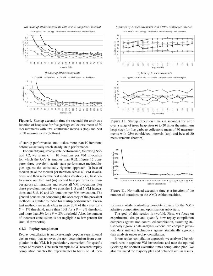
(a) mean of 30 measurements with a 95% confidence interval
55.25.45.65.8
66.26.46.66.8
7
32 40 48 56 64 72 80 88 96 104
112
120
128
136
144
152
160
168
176
184
192
heap size (MB)
exec
utio
n tim
e (s
)
CopyMS GenCopy GenMS MarkSweep SemiSpace
(b) best of 30 measurements
5
5.5
6
6.5
7
7.5
8
32 40 48 56 64 72 80 88 96 104
112
120
128
136
144
152
160
168
176
184
192
heap size (MB)
exec
utio
n tim
e (s
)
CopyMS GenCopy GenMS MarkSweep SemiSpace
Figure 9. Startup execution time (in seconds) for antlr as afunction of heap size for five garbage collectors; mean of 30measurements with 95% confidence intervals (top) and bestof 30 measurements (bottom).
of startup performance, and it takes more than 10 iterationsbefore we actually reach steady-state performance.
For quantifying steady-state performance, following Sec-tion 4.2, we retain k = 10 iterations per VM invocationfor which the CoV is smaller than 0.02. Figure 12 com-pares three prevalent steady-state performance methodolo-gies against the statistically rigorous approach: (i) best ofmedian (take the median per iteration across all VM invoca-tions, and then select the best median iteration), (ii) best per-formance number, and (iii) second best performance num-ber across all iterations and across all VM invocations. Forthese prevalent methods we consider 1, 3 and 5 VM invoca-tions and 3, 5, 10 and 30 iterations per VM invocation. Thegeneral conclusion concerning the accuracy of the prevalentmethods is similar to those for startup performance. Preva-lent methods are misleading in more 20% of the cases for aθ = 1% threshold, more than 10% for a θ = 2% threshold,and more than 5% for a θ = 3% threshold. Also, the numberof incorrect conclusions is not negligible (a few percent forsmall θ thresholds).
6.2.3 Replay compilationReplay compilation is an increasingly popular experimentaldesign setup that removes the non-determinism from com-pilation in the VM. It is particularly convenient for specifictopics of research. One such example is GC research: replaycompilation enables the experimenter to focus on GC per-
(a) mean of 30 measurements with a 95% confidence interval
55.15.25.35.45.55.65.75.8
192
224
256
288
320
352
384
416
448
480
512
544
576
608
640
heap size (MB)
exec
utio
n tim
e (s
)
CopyMS GenCopy GenMS MarkSweep SemiSpace
(b) best of 30 measurements
55.15.25.35.45.55.65.75.8
192
224
256
288
320
352
384
416
448
480
512
544
576
608
640
heap size (MB)ex
ecut
ion
time
(s)
CopyMS GenCopy GenMS MarkSweep SemiSpace
Figure 10. Startup execution time (in seconds) for antlrover a range of large heap sizes (6 to 20 times the minimumheap size) for five garbage collectors; mean of 30 measure-ments with 95% confidence intervals (top) and best of 30measurements (bottom).
0.65
0.70
0.75
0.80
0.85
0.90
0.95
1.00
1 2 3 4 5 6 7 8 9 10 11 12 13 14 15 16 17 18 19 20 21 22 23 24 25 26 27 28 29 30
number of iterations
norm
aliz
ed e
xecu
tion
time
Figure 11. Normalized execution time as a function of thenumber of iterations on the AMD Athlon machine.
formance while controlling non-determinism by the VM’sadaptive compilation and optimization subsystem.
The goal of this section is twofold. First, we focus onexperimental design and quantify how replay compilationcompares against non-controlled compilation, assuming sta-tistically rigorous data analysis. Second, we compare preva-lent data analysis techniques against statistically rigorousdata analysis under replay compilation.
In our replay compilation approach, we analyze 7 bench-mark runs in separate VM invocations and take the optimal(yielding the shortest execution time) compilation plan. Wealso evaluated the majority plan and obtained similar results.
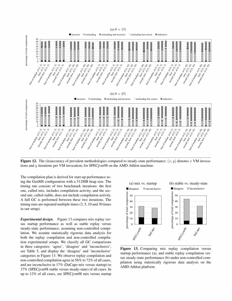
(a) θ = 1%
05
1015202530354045
best
of m
edian
of (
1, 3)
best
of (1
, 3)
seco
nd_b
est
of (1
, 3)
best
of m
edian
of (
1, 5)
best
of (1
, 5)
seco
nd_b
est
of (1
, 5)
best
of m
edian
of (
1, 10
)be
st of
(1, 1
0)
seco
nd_b
est
of (1
, 10)
best
of m
edian
of (
1, 30
)be
st of
(1, 3
0)
seco
nd_b
est
of (1
, 30)
best
of m
edian
of (
3, 3)
best
of (3
, 3)
seco
nd_b
est
of (3
, 3)
best
of m
edian
of (
3, 5)
best
of (3
, 5)
seco
nd_b
est
of (3
, 5)
best
of m
edian
of (
3, 10
)be
st of
(3, 1
0)
seco
nd_b
est
of (3
, 10)
best
of m
edian
of (
3, 30
)be
st of
(3, 3
0)
seco
nd_b
est
of (3
, 30)
best
of m
edian
of (
5, 3)
best
of (5
, 3)
seco
nd_b
est
of (5
, 3)
best
of m
edian
of (
5, 5)
best
of (5
, 5)
seco
nd_b
est
of (5
, 5)
best
of m
edian
of (
5, 10
)be
st of
(5, 1
0)
seco
nd_b
est
of (5
, 10)
best
of m
edian
of (
5, 30
)be
st of
(5, 3
0)
seco
nd_b
est
of (5
, 30)pe
rcen
tage
of t
otal
com
paris
ons incorrect misleading misleading and incorrect misleading but correct indicative
(b) θ = 2%
05
101520253035404550
best
of m
edian
of (
1, 3)
best
of (1
, 3)
seco
nd_b
est
of (1
, 3)
best
of m
edian
of (
1, 5)
best
of (1
, 5)
seco
nd_b
est
of (1
, 5)
best
of m
edian
of (
1, 10
)be
st of
(1, 1
0)
seco
nd_b
est
of (1
, 10)
best
of m
edian
of (
1, 30
)be
st of
(1, 3
0)
seco
nd_b
est
of (1
, 30)
best
of m
edian
of (
3, 3)
best
of (3
, 3)
seco
nd_b
est
of (3
, 3)
best
of m
edian
of (
3, 5)
best
of (3
, 5)
seco
nd_b
est
of (3
, 5)
best
of m
edian
of (
3, 10
)be
st of
(3, 1
0)
seco
nd_b
est
of (3
, 10)
best
of m
edian
of (
3, 30
)be
st of
(3, 3
0)
seco
nd_b
est
of (3
, 30)
best
of m
edian
of (
5, 3)
best
of (5
, 3)
seco
nd_b
est
of (5
, 3)
best
of m
edian
of (
5, 5)
best
of (5
, 5)
seco
nd_b
est
of (5
, 5)
best
of m
edian
of (
5, 10
)be
st of
(5, 1
0)
seco
nd_b
est
of (5
, 10)
best
of m
edian
of (
5, 30
)be
st of
(5, 3
0)
seco
nd_b
est
of (5
, 30)pe
rcen
tage
of t
otal
com
paris
ons incorrect misleading misleading and incorrect misleading but correct indicative
Figure 12. The (in)accuracy of prevalent methodologies compared to steady-state performance: (x, y) denotes x VM invoca-tions and y iterations per VM invocation; for SPECjvm98 on the AMD Athlon machine.
The compilation plan is derived for start-up performance us-ing the GenMS configuration with a 512MB heap size. Thetiming run consists of two benchmark iterations: the firstone, called mix, includes compilation activity, and the sec-ond one, called stable, does not include compilation activity.A full GC is performed between these two iterations. Thetiming runs are repeated multiple times (3, 5, 10 and 30 timesin our setup).
Experimental design. Figure 13 compares mix replay ver-sus startup performance as well as stable replay versussteady-state performance, assuming non-controlled compi-lation. We assume statistically rigorous data analysis forboth the replay compilation and non-controlled compila-tion experimental setups. We classify all GC comparisonsin three categories: ‘agree’, ‘disagree’ and ‘inconclusive’,see Table 5, and display the ‘disagree’ and ‘inconclusive’categories in Figure 13. We observe replay compilation andnon-controlled compilation agree in 56% to 72% of all cases,and are inconclusive in 17% (DaCapo mix versus startup) to37% (SPECjvm98 stable versus steady-state) of all cases. Inup to 12% of all cases, see SPECjvm98 mix versus startup
(a) mix vs. startup (b) stable vs. steady-state
0
10
20
30
40
50
SPEC
jvm
98
DaCa
po
perc
enta
ge o
f tot
al c
ompa
rison
s
disagree inconclusive
0
10
20
30
40
50
SPEC
jvm
98
DaCa
po
perc
enta
ge o
f tot
al c
ompa
rison
s
disagree inconclusive
Figure 13. Comparing mix replay compilation versusstartup performance (a), and stable replay compilation ver-sus steady-state performance (b) under non-controlled com-pilation using statistically rigorous data analysis on theAMD Athlon platform.
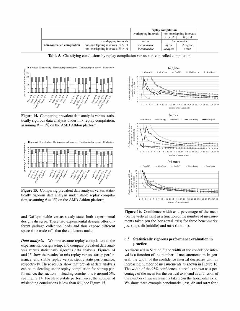
replay compilationoverlapping intervals non-overlapping intervals
A > B B > A
non-controlled compilationoverlapping intervals agree inconclusive
non-overlapping intervals, A > B inconclusive agree disagreenon-overlapping intervals, B > A inconclusive disagree agree
Table 5. Classifying conclusions by replay compilation versus non-controlled compilation.
0
5
10
15
20
25
best
of 3
mea
n of 3
med
ian of
3se
cond
_bes
t of 3
worst
of 3
best
of 5
mea
n of 5
med
ian of
5se
cond
_bes
t of 5
worst
of 5
best
of 10
mea
n of 1
0m
edian
of 10
seco
nd_b
est o
f 10
worst
of 10
best
of 30
mea
n of 3
0m
edian
of 30
seco
nd_b
est o
f 30
worst
of 30pe
rcen
tage
of t
otal
com
paris
ons incorrect misleading misleading and incorrect misleading but correct indicative
Figure 14. Comparing prevalent data analysis versus statis-tically rigorous data analysis under mix replay compilation,assuming θ = 1% on the AMD Athlon platform.
02468
101214161820
best
of 3
mea
n of 3
med
ian of
3se
cond
_bes
t of 3
worst
of 3
best
of 5
mea
n of 5
med
ian of
5se
cond
_bes
t of 5
worst
of 5
best
of 10
mea
n of 1
0m
edian
of 10
seco
nd_b
est o
f 10
worst
of 10
best
of 30
mea
n of 3
0m
edian
of 30
seco
nd_b
est o
f 30
worst
of 30pe
rcen
tage
of t
otal
com
paris
ons incorrect misleading misleading and incorrect misleading but correct indicative
Figure 15. Comparing prevalent data analysis versus statis-tically rigorous data analysis under stable replay compila-tion, assuming θ = 1% on the AMD Athlon platform.
and DaCapo stable versus steady-state, both experimentaldesigns disagree. These two experimental designs offer dif-ferent garbage collection loads and thus expose differentspace-time trade-offs that the collectors make.
Data analysis. We now assume replay compilation as theexperimental design setup, and compare prevalent data anal-ysis versus statistically rigorous data analysis. Figures 14and 15 show the results for mix replay versus startup perfor-mance, and stable replay versus steady-state performance,respectively. These results show that prevalent data analysiscan be misleading under replay compilation for startup per-formance: the fraction misleading conclusions is around 5%,see Figure 14. For steady-state performance, the number ofmisleading conclusions is less than 4%, see Figure 15.
(a) jess
0123456789
10
2 3 4 5 6 7 8 9 10 11 12 13 14 15 16 17 18 19 20 21 22 23 24 25 26 27 28 29 30number of measurements
conf
iden
ce in
terv
al w
idth
as a
pe
rcen
tage
of t
he m
ean
exec
utio
n tim
e
CopyMS GenCopy GenMS MarkSweep SemiSpace
(b) db
0123456789
10
2 3 4 5 6 7 8 9 10 11 12 13 14 15 16 17 18 19 20 21 22 23 24 25 26 27 28 29 30number of measurements
Con
fiden
ce in
terv
al w
idth
as a
pe
rcen
tage
of t
he m
ean
exec
utio
n tim
e
CopyMS GenCopy GenMS MarkSweep SemiSpace
(c) mtrt
0123456789
10
2 3 4 5 6 7 8 9 10 11 12 13 14 15 16 17 18 19 20 21 22 23 24 25 26 27 28 29 30number of measurements
Con
fiden
ce in
terv
al w
idth
as a
pe
rcen
tage
of t
he m
ean
exec
utio
n tim
e
CopyMS GenCopy GenMS MarkSweep SemiSpace
Figure 16. Confidence width as a percentage of the mean(on the vertical axis) as a function of the number of measure-ments taken (on the horizontal axis) for three benchmarks:jess (top), db (middle) and mtrt (bottom).
6.3 Statistically rigorous performance evaluation inpractice
As discussed in Section 3, the width of the confidence inter-val is a function of the number of measurements n. In gen-eral, the width of the confidence interval decreases with anincreasing number of measurements as shown in Figure 16.The width of the 95% confidence interval is shown as a per-centage of the mean (on the vertical axis) and as a function ofthe number of measurements taken (on the horizontal axis).We show three example benchmarks: jess, db and mtrt for a
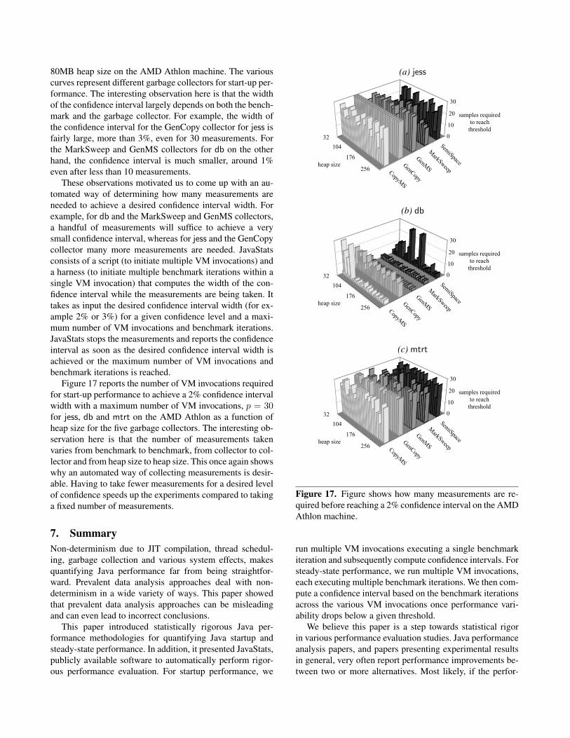
80MB heap size on the AMD Athlon machine. The variouscurves represent different garbage collectors for start-up per-formance. The interesting observation here is that the widthof the confidence interval largely depends on both the bench-mark and the garbage collector. For example, the width ofthe confidence interval for the GenCopy collector for jess isfairly large, more than 3%, even for 30 measurements. Forthe MarkSweep and GenMS collectors for db on the otherhand, the confidence interval is much smaller, around 1%even after less than 10 measurements.
These observations motivated us to come up with an au-tomated way of determining how many measurements areneeded to achieve a desired confidence interval width. Forexample, for db and the MarkSweep and GenMS collectors,a handful of measurements will suffice to achieve a verysmall confidence interval, whereas for jess and the GenCopycollector many more measurements are needed. JavaStatsconsists of a script (to initiate multiple VM invocations) anda harness (to initiate multiple benchmark iterations within asingle VM invocation) that computes the width of the con-fidence interval while the measurements are being taken. Ittakes as input the desired confidence interval width (for ex-ample 2% or 3%) for a given confidence level and a maxi-mum number of VM invocations and benchmark iterations.JavaStats stops the measurements and reports the confidenceinterval as soon as the desired confidence interval width isachieved or the maximum number of VM invocations andbenchmark iterations is reached.
Figure 17 reports the number of VM invocations requiredfor start-up performance to achieve a 2% confidence intervalwidth with a maximum number of VM invocations, p = 30for jess, db and mtrt on the AMD Athlon as a function ofheap size for the five garbage collectors. The interesting ob-servation here is that the number of measurements takenvaries from benchmark to benchmark, from collector to col-lector and from heap size to heap size. This once again showswhy an automated way of collecting measurements is desir-able. Having to take fewer measurements for a desired levelof confidence speeds up the experiments compared to takinga fixed number of measurements.
7. SummaryNon-determinism due to JIT compilation, thread schedul-ing, garbage collection and various system effects, makesquantifying Java performance far from being straightfor-ward. Prevalent data analysis approaches deal with non-determinism in a wide variety of ways. This paper showedthat prevalent data analysis approaches can be misleadingand can even lead to incorrect conclusions.
This paper introduced statistically rigorous Java per-formance methodologies for quantifying Java startup andsteady-state performance. In addition, it presented JavaStats,publicly available software to automatically perform rigor-ous performance evaluation. For startup performance, we
(a) jess
32104
176
256 CopyMS
GenCopy
GenMS
MarkSweep
SemiSpace
0
10
20
30
samples required to reach
threshold
heap size
(b) db
32104
176
256 CopyMS
GenCopy
GenMS
MarkSweep
SemiSpace
0
10
20
30
samples required to reach
threshold
heap size
(c) mtrt
32104
176
256 CopyMS
GenCopy
GenMS
MarkSweep
SemiSpace
0
10
20
30
samples required to reach
threshold
heap size
Figure 17. Figure shows how many measurements are re-quired before reaching a 2% confidence interval on the AMDAthlon machine.
run multiple VM invocations executing a single benchmarkiteration and subsequently compute confidence intervals. Forsteady-state performance, we run multiple VM invocations,each executing multiple benchmark iterations. We then com-pute a confidence interval based on the benchmark iterationsacross the various VM invocations once performance vari-ability drops below a given threshold.
We believe this paper is a step towards statistical rigorin various performance evaluation studies. Java performanceanalysis papers, and papers presenting experimental resultsin general, very often report performance improvements be-tween two or more alternatives. Most likely, if the perfor-
mance differences between the alternatives are large, a sta-tistically rigorous method will not alter the overall picturenor affect the general conclusions obtained using prevalentmethods. However, for relatively small performance differ-ences (that are within the margin of experimental error), notusing statistical rigor may lead to incorrect conclusions.
AcknowledgmentsWe would like to thank Steve Blackburn, Michael Hind,Matthew Arnold, Kathryn McKinley, and the anonymousreviewers for their valuable comments — their detailedsuggestions greatly helped us improving this paper. AndyGeorges is supported by Ghent University. Dries Buytaertis supported by the Institute for the Promotion of Innova-tion by Science and Technology in Flanders (IWT). LievenEeckhout is a Postdoctoral Fellow of the Fund for ScientificResearch–Flanders (Belgium) (FWO–Vlaanderen).
References[1] M. Arnold, S. Fink, D. Grove, M. Hind, and P. F. Sweeney.
Adaptive optimization in the Jalapeno JVM. In OOPSLA,pages 47–65, Oct. 2000.
[2] M. Arnold, M. Hind, and B. G. Ryder. Online feedback-directed optimization of Java. In OOPSLA, pages 111–129,Nov. 2002.
[3] K. Barabash, Y. Ossia, and E. Petrank. Mostly concurrentgarbage collection revisited. In OOPSLA, pages 255–268,Nov. 2003.
[4] O. Ben-Yitzhak, I. Goft, E. K. Kolodner, K. Kuiper, andV. Leikehman. An algorithm for parallel incrementalcompaction. In ISMM, pages 207–212, Feb. 2003.
[5] S. Blackburn, P. Cheng, and K. McKinley. Myths andreality: The performance impact of garbage collection. InSIGMETRICS, pages 25–36, June 2004.
[6] S. Blackburn, P. Cheng, and K. McKinley. Oil and water?High performance garbage collection in Java with JMTk. InICSE, pages 137–146, May 2004.
[7] S. M. Blackburn, R. Garner, C. Hoffmann, A. M. Khang, K. S.McKinley, R. Bentzur, A. Diwan, D. Feinberg, D. Frampton,S. Z. Guyer, M. Hirzel, A. Hosking, M. Jump, H. Lee, J. E. B.Moss, A. Phansalkar, D. Stefanovic, T. VanDrunen, D. vonDincklage, and B. Wiedermann. The DaCapo benchmarks:Java benchmarking development and analysis. In OOPSLA,pages 169–190, Oct. 2006.
[8] S. M. Blackburn and K. S. McKinley. In or out?: Puttingwrite barriers in their place. In ISMM, pages 281–290, June2002.
[9] S. M. Blackburn and K. S. McKinley. Ulterior reference
counting: Fast garbage collection without a long wait. InOOPSLA, pages 344–358, Oct. 2003.
[10] L. Eeckhout, A. Georges, and K. De Bosschere. How Javaprograms interact with virtual machines at the microarchitec-tural level. In OOPSLA, pages 169–186, Oct. 2003.
[11] D. Gu, C. Verbrugge, and E. M. Gagnon. Relative factorsin performance analysis of Java virtual machines. In VEE,pages 111–121, June 2006.
[12] M. Hauswirth, P. F. Sweeney, A. Diwan, and M. Hind.Vertical profiling: Understanding the behavior of object-priented applications. In OOPSLA, pages 251–269, Oct.2004.
[13] J.L. Hintze, and R.D. Nelson. Violin Plots: A Box Plot-Density Trace Synergism In The American Statistician,Volume 52(2), pages 181–184, May 1998.
[14] X. Huang, S. M. Blackburn, K. S. McKinley, J. E. B. Moss,Z. Wang, and P. Cheng. The garbage collection advantage:Improving program locality. In OOPSLA, pages 69–80, Oct.2004.
[15] R.A. Johnson and D.W. Wichern Applied MultivariateStatistical Analysis Prentice Hall, 2002
[16] D. J. Lilja. Measuring Computer Performance: A Practi-tioner’s Guide. Cambridge University Press, 2000.
[17] J. Maebe, D. Buytaert, L. Eeckhout, and K. De Bosschere.Javana: A system for building customized Java programanalysis tools. In OOPSLA, pages 153–168, Oct. 2006.
[18] P. McGachey and A. L. Hosking. Reducing generational copyreserve overhead with fallback compaction. In ISMM, pages17–28, June 2006.
[19] J. Neter, M. H. Kutner, W. Wasserman, and C. J. NachtsheimApplied Linear Statistical Models WCB/McGraw-Hill, 1996.
[20] N. Sachindran and J. E. B. Moss. Mark-copy: Fast copyingGC with less space overhead. In OOPSLA, pages 326–343,Oct. 2003.
[21] K. Sagonas and J. Wilhelmsson. Mark and split. In ISMM,pages 29–39, June 2006.
[22] D. Siegwart and M. Hirzel. Improving locality with parallelhierarchical copying GC. In ISMM, pages 52–63, June 2006.
[23] Standard Performance Evaluation Corporation. SPECjvm98Benchmarks. http://www.spec.org/jvm98.
[24] P. F. Sweeney, M. Hauswirth, B. Cahoon, P. Cheng, A. Diwan,D. Grove, and M. Hind. Using hardware performancemonitors to understand the behavior of Java applications.In VM, pages 57–72, May 2004.
[25] C. Zhang, K. Kelsey, X. Shen, C. Ding, M. Hertz, andM. Ogihara. Program-level adaptive memory management.In ISMM, pages 174–183, June 2006.
Related Documents